hardness of approximation between p and np...hardness of approximation between p and np aviad...
TRANSCRIPT

Hardness of Approximation Between P and NP
Aviad Rubinstein
Electrical Engineering and Computer SciencesUniversity of California at Berkeley
Technical Report No. UCB/EECS-2017-146http://www2.eecs.berkeley.edu/Pubs/TechRpts/2017/EECS-2017-146.html
August 11, 2017

Copyright © 2017, by the author(s).All rights reserved.
Permission to make digital or hard copies of all or part of this work forpersonal or classroom use is granted without fee provided that copies arenot made or distributed for profit or commercial advantage and that copiesbear this notice and the full citation on the first page. To copy otherwise, torepublish, to post on servers or to redistribute to lists, requires prior specificpermission.

Hardness of Approximation Between P and NP
by
Aviad Rubinstein
A dissertation submitted in partial satisfaction of the
requirements for the degree of
Doctor of Philosophy
in
Computer Science
in the
Graduate Division
of the
University of California, Berkeley
Committee in charge:
Professor Christos Papadimitriou, ChairProfessor Ilan Adler
Associate Professor Prasad RaghavendraProfessor Satish Rao
Summer 2017

The dissertation of Aviad Rubinstein, titled Hardness of Approximation BetweenP and NP, is approved:
Chair Date
Date
Date
Date
University of California, Berkeley

Hardness of Approximation Between P and NP
Copyright 2017by
Aviad Rubinstein

1
Abstract
Hardness of Approximation Between P and NP
by
Aviad Rubinstein
Doctor of Philosophy in Computer Science
University of California, Berkeley
Professor Christos Papadimitriou, Chair
Nash equilibrium is the central solution concept in Game Theory. Since Nash’s orig-inal paper in 1951, it has found countless applications in modeling strategic behaviorof traders in markets, (human) drivers and (electronic) routers in congested networks,nations in nuclear disarmament negotiations, and more. A decade ago, the relevanceof this solution concept was called into question by computer scientists [DGP09;CDT09], who proved (under appropriate complexity assumptions) that computing aNash equilibrium is an intractable problem. And if centralized, specially designedalgorithms cannot find Nash equilibria, why should we expect distributed, selfishagents to converge to one? The remaining hope was that at least approximate Nashequilibria can be efficiently computed.
Understanding whether there is an efficient algorithm for approximate Nash equi-librium has been the central open problem in this field for the past decade. In thisthesis, we provide strong evidence that even finding an approximate Nash equilibriumis intractable. We prove several intractability theorems for different settings (two-player games and many-player games) and models (computational complexity, querycomplexity, and communication complexity). In particular, our main result is thatunder a plausible and natural complexity assumption (“Exponential Time Hypoth-esis for PPAD”), there is no polynomial-time algorithm for finding an approximateNash equilibrium in two-player games.
The problem of approximate Nash equilibrium in a two-player game poses aunique technical challenge: it is a member of the class PPAD, which captures thecomplexity of several fundamental total problems, i.e. problems that always havea solution; and it also admits a quasipolynomial (≈ nlogn) time algorithm. Eitherproperty alone is believed to place this problem far below NP-hard problems in thecomplexity hierarchy; having both simultaneously places it just above P, at what can

2
be called the frontier of intractability. Indeed, the tools we develop in this thesis toadvance on this frontier are useful for proving hardness of approximation of severalother important problems whose complexity lies between P and NP:
Brouwer’s fixed point Given a continuous function f mapping a compact convexset to itself, Brouwer’s fixed point theorem guarantees that f has a fixed point,i.e. x such that f(x) = x. Our intractability result holds for the relaxed problemof finding an approximate fixed point, i.e. x such that f(x) ≈ x.
Market equilibrium Market equilibrium is a vector of prices and allocations wherethe supply meets the demand for each good. Our intractability result holds forthe relaxed problem of finding an approximate market equilibrium, where thesupply of each good approximately meets the demand.
CourseMatch (A-CEEI) Approximate Competitive Equilibrium from Equal In-come (A-CEEI) is the economic principle underlying CourseMatch, a systemfor fair allocation of classes to students (currently in use at Wharton, Universityof Pennsylvania).
Densest k-subgraph Our intractability result holds for the following relaxation ofthe k-Clique problem: given a graph containing a k-clique, the algorithm hasto find a subgraph over k vertices that is “almost a clique”, i.e. most of theedges are present.
Community detection We consider a well-studied model of communities in socialnetworks, where each member of the community is friends with a large fractionof the community, and each non-member is only friends with a small fractionof the community.
VC dimension and Littlestone dimension The Vapnik-Chervonenkis (VC) di-mension is a fundamental measure in learning theory that captures the com-plexity of a binary concept class. Similarly, the Littlestone dimension is ameasure of complexity of online learning.
Signaling in zero-sum games We consider a fundamental problem in signaling,where an informed signaler reveals private information about the payoffs in atwo-player zero-sum game, with the goal of helping one of the players.

i

ii
Contents
Contents ii
List of Figures v
List of Tables vi
I Overview 1
1 The frontier of intractability 21.1 PPAD: Finding a needle you know is in the haystack . . . . . . . . . . 41.2 Quasi-polynomial time and the birthday paradox . . . . . . . . . . . . 111.3 Approximate Nash equilibrium . . . . . . . . . . . . . . . . . . . . . . . 16
2 Preliminaries 182.1 Nash equilibrium and relaxations . . . . . . . . . . . . . . . . . . . . . . 182.2 PPAD and End-of-a-Line . . . . . . . . . . . . . . . . . . . . . . . . . . 202.3 Exponential Time Hypotheses . . . . . . . . . . . . . . . . . . . . . . . . 212.4 PCP theorems . . . . . . . . . . . . . . . . . . . . . . . . . . . . . . . . . 212.5 Learning Theory . . . . . . . . . . . . . . . . . . . . . . . . . . . . . . . . 232.6 Information Theory . . . . . . . . . . . . . . . . . . . . . . . . . . . . . . 242.7 Useful lemmata . . . . . . . . . . . . . . . . . . . . . . . . . . . . . . . . . 26
II Communication Complexity 30
3 Communication Complexity of approximate Nash equilibrium 313.1 Proof overview . . . . . . . . . . . . . . . . . . . . . . . . . . . . . . . . . 373.2 Proofs . . . . . . . . . . . . . . . . . . . . . . . . . . . . . . . . . . . . . . 413.3 An open problem: correlated equilibria in 2-player games . . . . . . . . 57

iii
4 Brouwer’s fixed point 584.1 Brouwer with `∞ . . . . . . . . . . . . . . . . . . . . . . . . . . . . . . . 584.2 Euclidean Brouwer . . . . . . . . . . . . . . . . . . . . . . . . . . . . . 64
III PPAD 74
5 PPAD-hardness of approximation 75
6 The generalized circuit problem 786.1 Proof overview . . . . . . . . . . . . . . . . . . . . . . . . . . . . . . . . . 806.2 From Brouwer to ε-Gcircuit . . . . . . . . . . . . . . . . . . . . . . . . 826.3 Gcrcuit with Fan-out 2 . . . . . . . . . . . . . . . . . . . . . . . . . . . 98
7 Many-player games 1017.1 Graphical, polymatrix games . . . . . . . . . . . . . . . . . . . . . . . . . 1017.2 Succinct games . . . . . . . . . . . . . . . . . . . . . . . . . . . . . . . . . 107
8 Bayesian Nash equilibrium 111
9 Market Equilibrium 1149.1 Non-monotone markets: proof of inapproximability . . . . . . . . . . . 118
10 Course Match 13010.1 The Course Allocation Problem . . . . . . . . . . . . . . . . . . . . . . . 13210.2 A-CEEI is PPAD-hard . . . . . . . . . . . . . . . . . . . . . . . . . . . . . 13410.3 A-CEEI ∈ PPAD . . . . . . . . . . . . . . . . . . . . . . . . . . . . . . . . 140
IV Quasi-polynomial Time 147
11 Birthday repetition 14811.1 Warm-up: best ε-Nash . . . . . . . . . . . . . . . . . . . . . . . . . . . . . 149
12 Densest k-Subgraph 15412.1 Construction (and completeness) . . . . . . . . . . . . . . . . . . . . . . 15812.2 Soundness . . . . . . . . . . . . . . . . . . . . . . . . . . . . . . . . . . . . 159
13 Community detection 17713.1 Hardness of counting communities . . . . . . . . . . . . . . . . . . . . . 18213.2 Hardness of detecting communities . . . . . . . . . . . . . . . . . . . . . 184

iv
14 VC and Littlestone’s dimensions 18814.1 Inapproximability of VC Dimension . . . . . . . . . . . . . . . . . . . . . 19214.2 Inapproximability of Littlestone’s Dimension . . . . . . . . . . . . . . . 20014.3 Quasi-polynomial Algorithm for Littlestone’s Dimension . . . . . . . . 211
15 Signaling 21415.1 Near-optimal signaling is hard . . . . . . . . . . . . . . . . . . . . . . . . 216
V Approximate Nash Equilibrium 222
16 2-Player approximate Nash Equilibrium 22316.1 Technical overview . . . . . . . . . . . . . . . . . . . . . . . . . . . . . . . 22516.2 End-of-a-Line with local computation . . . . . . . . . . . . . . . . . . 23216.3 Holographic Proof . . . . . . . . . . . . . . . . . . . . . . . . . . . . . . . 23516.4 Polymatrix WeakNash . . . . . . . . . . . . . . . . . . . . . . . . . . . . 24816.5 From polymatrix to bimatrix . . . . . . . . . . . . . . . . . . . . . . . . . 268
Bibliography 273

v
List of Figures
4.1 A facet of the Hirsch et al construction . . . . . . . . . . . . . . . . . . . . . 634.2 Outside the picture . . . . . . . . . . . . . . . . . . . . . . . . . . . . . . . . . 644.3 Geometry near a Brouwer vertex . . . . . . . . . . . . . . . . . . . . . . . . 71
6.1 Comparison of averaging gadgets . . . . . . . . . . . . . . . . . . . . . . . . 81
14.1 Reduction from Label Cover to VC Dimension . . . . . . . . . . . . . . . . 21214.2 Reduction from Label Cover to Littlestone’s Dimension . . . . . . . . . . . 213

vi
List of Tables
9.1 Goods and traders . . . . . . . . . . . . . . . . . . . . . . . . . . . . . . . . . 124
15.1 Variables in proof of Theorem 15.1.1 . . . . . . . . . . . . . . . . . . . . . . 218

vii
Acknowledgments
I am incredibly lucky to have Christos as my advisor. I cannot compete with thepraise written in dozens of Acknowledgment Sections in the dissertations of previousstudents of Christos. I can only attest that it’s all true. Christos, thank you forgiving me beautiful problems to think about, for sprinkling your magic over myintroductions, for the pre-deadline nights, and for showing me around Greece (inparticular, Ikaria). Most importantly, thanks for all the advice!
I also thank my thesis committee, Ilan Adler, Prasad Raghavendra, Satish Rao,and Christos. Their feedback during my qualifying exam was already tremendouslyhelpful, and was my starting point for the last two parts of my thesis.
For the past few years it has been a great pleasure to belong to the theory groupat Berkeley. The lunches, retreats, basketball and soccer games, and occasional talkswere an excellent inspiration. In particular, I was extremely fortunate to be part ofthe office: Jonah Brown-Cohen, Rishi Gupta, Alex Psomas, Tselil Schramm, JarettSchwartz, Ning Tan, Ben Weitz, thanks!
The latest perk of being a theorist at Berkeley is the Simons Institute. Eachsemester brings an influx of fascinating new and old visitors and learning oppor-tunities. Indeed, much of this thesis was first written on the white boards in thecollaboration area. Thanks Dick Karp, Christos, Alistair Sinclair, Luca Trevisan,program organizers, and the Simons Foundation for spoiling me.
Before coming to Berkeley, I was particularly influenced by long conversationswith Elad Haramaty and my M.Sc. advisor Muli Safra. I don’t believe I would bedoing theory if it weren’t for Muli; I probably would not be in academia at all if itweren’t for Elad.
I am grateful to Microsoft Research for the MSR PhD Fellowship, as well aswonderful summer internships, where I had the fortune to learn from Moshe Babaioff,Siu On Chan, Wei Chen, Jason Hartline, Bobby Kleinberg, Nicole Immorlica, PinyanLu, Brendan Lucier, Yishay Mansour, Noam Nisan, Moshe Tennenholtz, and manyothers. I also thank Mark Braverman, Michal Feldman, Noam Nisan, and YaronSinger for hosting me for shorter visits during my PhD.
I am also grateful to all my coauthors: Amir Abboud, Ilan Adler, Yakov Babichenko,Ashwin Badanidiyuru, Eric Balkanski, Mark Braverman, Siu On Chan, Wei Chen,Michal Feldman, Ophir Friedler, Young Kun Ko, Fu Li, Tian Lin, Adi Livnat,Yishay Mansour, Pasin Manurangsi, Abe Othman, Christos, Dimitris Papailiopoulos,George Pierrakos, Alex, Tselil, Lior Seeman, Yaron Singer, Sahil Singla, Moshe Ten-nenholtz, Greg Valiant, Shai Vardi, Andrew Wan, Matt Weinberg, Omri Weinstein,and Ryan Williams.

viii
Thanks also to Boaz Barak, Shai Ben-David, Jonah, Karthik C.S., Yang Cai,Alessandro Chiesa, Paul Christiano, Constantinos Daskalakis, Shaddin Dughmi,Mika Goos, Rishi, Elad, Noam, Prasad, Tselil, Madhu Sudan, Luca Trevisan, MichaelViderman, and anonymous reviewers, for commenting on, correcting, and inspiringmuch of the content of this thesis.
This has been an amazing journey. I am most grateful for the opportunities Ihad to share it with my family and friends.

1
Part I
Overview

2
Chapter 1
The frontier of intractability
The combination of vast amounts of data, unprecedented computing power, andclever algorithms allows today’s computer systems to drive autonomous cars, beatthe best human players at Chess and Go, and live stream videos of cute cats acrossthe world. Yet computers can fail miserably at predicting outcomes of social pro-cesses and interactions, elections being only the most salient example. And this ishardly surprising, as there are two potent reasons for such unpredictability: Onereason is that human agents are driven by emotions and hormones and billions ofneurons interacting with a complex environment, and as a result their behavior isextremely hard to model mathematically. The second reason is perhaps a bit surpris-ing, and certainly closer to the concerns of this thesis: Even very simple and idealizedmodels of social interaction, in which agents have extremely clear-cut objectives, canbe intractable.
To have any hope of reasoning about human behavior on national and globalscales, we need a mathematically sound theory. Game Theory is the mathematicaldiscipline that models and analyzes the interaction between agents (e.g. voters) whohave different goals and are affected by each other’s actions. The central solutionconcept in game theory is the Nash equilibrium. It has an endless list of applicationsin economics, politics, biology, etc. (e.g. [Aum87]).
By Nash’s theorem [Nas51], an equilibrium always exists. Furthermore, once ata Nash equilibrium, players have no incentive to deviate. The main missing piece inthe puzzle is:
How do players arrive at an equilibrium in the first place?
After many attempts by economists for more than six decades1 (e.g. [Bro51; Rob51;
1In fact, “more than six decades” is an understatement: Irving Fisher’s thesis from 1891 dealt

CHAPTER 1. THE FRONTIER OF INTRACTABILITY 3
LH64; Sha64; Sca67; KL93; HMC03; FY06]), we still don’t have a satisfying expla-nation.
About ten years ago, the study of this fundamental question found a surprisinganswer in computer science: Chen et al [CDT09] and Daskalakis et al [DGP09]proved that finding a Nash equilibrium is computationally intractable2. And if nocentralized, specialized algorithm can find an equilibrium, it is even less likely thatdistributed, selfish agents will naturally converge to one. This casts doubt over theentire solution concept.
For the past decade, the main remaining hope for Nash equilibrium has beenapproximation. The central open question in this field has been:
Is there an efficient algorithm for finding an approximate Nash equilib-rium?
In this thesis we give a strong negative resolution to this question: our main resultrules out efficient approximation algorithms for finding Nash equilibria3.
Our theorem is the latest development in a long and intriguing technical story.The first question we computer scientists ask when encountering a new algorithmicchallenge is: is it in P, the class of polynomial time (tractable) problems; or is itNP-hard, like Satisfiability and the Traveling Salesperson Problem (where the bestknown algorithms require exponential time)? Approximate Nash equilibrium fallsinto neither category; its complexity lies between P and NP-hard — hence the titleof our thesis. Let us introduce two (completely orthogonal) reasons why we do notexpect it to be NP-hard.
The first obstacle for NP-hardness is the totality of Nash equilibrium. When wesay that Satisfiability or the Traveling Salesperson Person problems are NP-hard,we formally mean that it is NP-hard to determine whether a given formula has asatisfying assignment, or whether a given network allows the salesperson to completeher travels within a certain budget. In contrast, by Nash’s theorem an equilibriumalways exists. Deciding whether an equilibrium exists is is trivial, but we still don’tknow how to find one. This is formally captured by an intermediate complexity classcalled PPAD.
The second obstacle for NP-hardness is an algorithm (the worst kind of obstaclefor intractability). The best known algorithms for solving NP-hard or PPAD-hardproblems require exponential (≈ 2n) time, and there is a common belief (formulated
with the closely related question of convergence to market equilibria [BS00].2Assuming P ≠ PPAD; see the discussion in the next section about this assumption.3Under a complexity assumption stronger than P ≠ PPAD, that we call the Exponential Time
Hypothesis (ETH) for PPAD, see Section 1.2 for details.

CHAPTER 1. THE FRONTIER OF INTRACTABILITY 4
a few years ago as the “Exponential Time Hypothesis” [IPZ01]) that much fasteralgorithms do not exist. In contrast, an approximate Nash equilibrium can be foundin quasi-polynomial (≈ nlogn) time. Notice that this again places the complexity ofapproximate Nash equilibrium between the polynomial time solvable problems inP and the exponential time required by NP-hard problems. Therefore, approximateNash equilibrium is unlikely to be NP-hard — or even PPAD-hard, since we know ofno quasi-polynomial algorithm for any other PPAD-hard problem.
As illustrated in the last two paragraphs, approximate Nash equilibrium is veryfar from our standard notion of intractability, NP-hardness. In some sense, it is oneof the computationally easiest problems which we can still prove to be intractable— it lies at the frontier of our understanding of intractability. Unsurprisingly, thetechniques we had to master to prove the intractability of approximate Nash equi-librium are useful for many other problems. In particular, we also prove hardness ofapproximation for several other interesting problems that either belong to the classPPAD or have quasi-polynomial time algorithms.
1.1 PPAD: Finding a needle you know is in the
haystack
Consider a directed graph G. Each edge contributes to the degree of the two verticesincident on it. Hence the sum of the degrees is twice the number of edges, and inparticular it is even. Now, given an odd-degree vertex v, there must exist anotherodd-degree vertex. But can you find one? There is, of course, the trivial algorithmwhich simply brute-force enumerates over all the graph vertices.
Now suppose G further has the property4 that every vertex has in- and out-degreeat most 1. Thus, G is a disjoint unions of lines and cycles. If v has an outgoing edgebut no incoming edge, it is the beginning of a line. Now the algorithm for findinganother odd degree node is a bit more clever — follow the path to the end — butits worst case is still linear in the number of nodes.
In the worst case, both algorithms run in time linear in the number of vertices.When the graph is given explicitly, e.g. as an adjacency matrix, this is quite efficientcompared to the size of the input. But what if the graph is given as black-box oraclesS and P that return, for each vertex, its successor and predecessor in the graph? The
4This guarantee is actually without loss of generality [Pap94], but this is not so important forour purposes.

CHAPTER 1. THE FRONTIER OF INTRACTABILITY 5
amount of work5 required for finding another odd-degree vertex by the exhaustivealgorithm, or the path-following algorithm, is still linear in the number of vertices,but now this number is exponential in the natural parameter of the problem, thelength of the input to the oracle, which equals the logarithm of the number of nodes.In the oracle model, it is not hard to prove that there are no better algorithms.
Let us consider the computational analog of the black-box oracle model: theoracles S and P are implemented as explicit (“white-box”) circuits, which are givenas the input to the algorithm. This is the End-of-a-Line problem, which is thestarting point for most of our reductions. The computational class PPAD (whichstands for Polynomial Parity Argument in Directed graphs) is the class of searchproblems reducible to End-of-a-Line.
Definition 1.1.1 (End-of-a-Line [DGP09]). Given two circuits S and P , with minput bits and m output bits each, such that P (0m) = 0m ≠ S (0m), find an inputx ∈ 0,1m such that P (S (x)) ≠ x or S (P (x)) ≠ x ≠ 0m.
How hard is End-of-a-Line? We believe that it is likely to be very hard, al-most as hard as the black-box variant. This belief is backed by relativized separations[Mor03] and cryptographic hardness [BPR15; GPS16; HY17], as well as zero algo-rithmic progress, even on special cases, since it was first introduced in [Pap94]. Moreimportantly, we are embarrassingly bad at gaining insight to a circuit functionalityby looking at its structure (with some notable exceptions in cryptography [Bar04])— hence it seems reasonable to conjecture that the white-box variant is easier thanthe black-box problem.
Even more embarrassing is our inability to prove computational intractability.Essentially all “proofs” of computational intractability (including the ones in thisthesis) are conditional; i.e. we assume that some problem is hard (e.g. End-of-a-Line or Satisfiability), and reduce it to a new problem we want to “prove” is hard.The intractability of the new problem only holds conditioned on the intractability ofthe original hard problem. Without first resolving whether P = NP, we cannot provethat End-of-a-Line is indeed hard. Furthermore, even merely proving that End-of-a-Line is NP-hard would already imply unlikely consequences like NP = coNP[MP91]. The ultimate reason we believe that End-of-a-Line is intractable is thatwe have no idea how to prove it.
Once we believe that End-of-a-Line is indeed intractable, any problem that isPPAD-complete, i.e. “at least as hard as End-of-a-Line” is also intractable. Thecelebrated works of [DGP09; CDT09] prove that finding an exact Nash equilibrium
5Here work is measured by the number of oracle calls rather than running time; indeed thismodel will be the starting point of our reductions for query and communication complexity.

CHAPTER 1. THE FRONTIER OF INTRACTABILITY 6
is PPAD-complete. In Section 1.3 we describe some variants of approximate Nashequilibrium that are also PPAD-complete.
We conclude this section with a few problems (other than variants of Nash equi-librium) that we show are also PPAD-hard:
• Finding an approximate fixed point of an implicit function; Brouwer’s fixedpoint theorem, which guarantees the existence of a fixed point, lays the math-ematical foundation for the rest of our PPAD-complete problems.
• Finding an approximate market equilibrium, which is the conceptual founda-tion of neoclassical economics.
• Finding an Approximate Competitive Equilibrium from Equal Incomes (A-CEEI), which is an algorithmic problem of practical interest due to its use forallocating classes to students (CourseMatch).
1.1.1 Brouwer’s fixed point
Brouwer’s fixed point theorem, together with its generalizations (in particular, Kaku-tani’s fixed point theorem), is the basis for many of the equilibrium concepts in gametheory and economics. It states that any continuous function f from a compact con-vex set (in particular, the n-dimensional hypercube) to itself has a fixed point, i.e.a point x∗ such that f (x∗) = x∗. Just like in the case of a Nash equilibrium and theodd-degree vertex, the existence does not come with an algorithm for finding the fixedpoint. Brouwer eventually became so unsatisfied with the non-constructive natureof his proof that he founded intuitionism, a formalism of mathematics mandatingconstructive proofs [Iem16].
Before we discuss the computational tractability of finding a fixed point, thereare two subtle but important technicalities that we have to clear. The first is thatfinding an exact fixed point may be “obviously” intractable when all the fixed pointsare irrational. Fortunately there is a natural notion6 of approximate fixed point: findx such that f (x) ≈ x. The second issue is that we want a finite description of theinput to our algorithm. Naively, one can define the value of the function on a grid,but then the set is no longer convex and a fixed point might not exist at all (seee.g. [RW16]). It turns out that a better way to define the input is as an arithmeticcircuit: this gives a local and easy-to-verify guarantee that the function is indeedcontinuous.
6There is also a stricter notion that requires x to be close to an x∗ for which f (x∗) = x∗ exactly.See e.g. [EY10].

CHAPTER 1. THE FRONTIER OF INTRACTABILITY 7
Admittedly, there is something dissatisfying about proving computational hard-ness of “circuit problems”: we are going to prove that this problem is PPAD-hard,i.e. no easier than End-of-a-Line — but the reason we believe in the first placethat End-of-a-Line is intractable is that we don’t know how to gain insight to thefunctionality of the circuit from staring at its structure. Nevertheless, we begin withthe complexity of Brouwer’s fixed point because: this is a fundamental question; itis the starting point of many of our reductions; and, as we discuss later, even theblack-box hardness in this case is highly non-trivial.
We know of two algorithms for computing approximate Brouwer fixed point:there is Scarf’s algorithm [Sca67], but its running time may be exponential in thedescription of the function; the same holds for brute-force search.
On the complexity side, [DGP09] proved that even in three dimensions, findingan exponentially-close approximation (x such that ∥f (x) − x∥∞ ≤ 2−n, where n isthe size of the input) is PPAD-complete; [CD09] proved the same problem continuesto be hard even with only two dimensions. Notice that with a constant number ofdimensions, any weaker approximation desideratum becomes trivial for brute-forcesearch. [CDT09] showed that in n dimensions, polynomial approximations are alsoPPAD-complete. We will later prove that even constant approximation are PPAD-complete, i.e. there exists some absolute constant ε > 0 such that it’s hard to findan x for which ∥f (x) − x∥∞ ≤ ε; this is already a significant improvement over theexisting state of the art.
We can prove an even stronger form of inapproximability for finding a Brouwerfixed point: so far, we characterized the approximate fixed point with `∞-norm,which means that f (x) and x must be close in every coordinates. Our main resultin this regard (Theorem 4.2.1) is that even if we only require that f (x) and x areclose in most of the coordinates, finding such x and f (x) remains PPAD-complete.
1.1.2 Market equilibrium
Supply and demand is central to our modern understanding of economics: whendemand exceeds supply, raising the price makes it less attractive to consumers andmore attractive to producers, thereby reducing demand and increasing supply. Viceversa if the supply exceeds the demand. This simple idea marks the birth of neo-classical economics [Jev66; Men71; Wal74], and continues to inspire us today whenwe reason about free market economy. Since the consumption and production of onegood depends on other goods, we are interested in a market equilibrium: a vector ofprices where the supply and demand of every good matches.
The supply and demand argument has many weak spots, one of which is Giffengoods [Mar95]: Consider a poor 19th century English family consuming a 10,000

CHAPTER 1. THE FRONTIER OF INTRACTABILITY 8
calories a day from meat and bread. They prefer to eat meat, but the bread ischeaper - so they spend their daily income on 6 loafs of bread and 4 pounds of meat(each provides 1,000 calories). What happens the price of bread increases? Theyhave less free money to spend on the luxury good (meat), which increases theirdemand for bread. The existence of Giffen goods in practice has been contentiouslydebated for over a century [Edg09; Sti47], with evidence ranging from econometricanalasys of historical market data to experiments in lab rats [BKK91].
Despite counter-intuitive issues like Giffen goods, Arrow and Debreu proved that,under quite general conditions, a market equilibrium always exists [DA54]. In par-ticular, in the Arrow-Debreu model, agents sell the goods they own and use therevenue to buy other goods they want; this is in contrast to Fisher markets whereagents with a monetary budget purchase from a centralized sellers. Market equilibriain both models exist, but can we find them? As in the case of Nash equilibrium, thisquestion is of particular importance because if a centralized, omniscient algorithmcannot compute an equilibrium, it is hard to expect a distributed market with selfishagents to converge to one. In the words of Kamal Jain [Jai04; Nis09b]:
“If your laptop cannot find it, neither can the market.”
In the same paper, Jain also gave an algorithm for computing Arrow-Debreu’s equi-librium when consumers utilities are linear. Since then, there has been a long se-quence of algorithms for computing or approximating market equilibria (e.g. [Jai04;CMV05; GK06; Dev+08; CF08; JV10; BDX11; Gar+15]) for certain models andutility functions, as well as intractability results in other settings [DD08; Che+09;VY11; Gar+17]. In particular, Chen, Paparas, and Yannakakis [CPY13] considera setting of markets which exhibit non-monotonicity: when the price of one prod-uct increases, its demand increases. Giffen goods described above are one exampleof non-monotone markets; [CPY13] construct examples in Arrow-Debreu marketswhen the increased price of a product increases the revenue of the seller, who nowhas more available money and demands more of the same good. Chen, Paparas,and Yannakakis [CPY13] show that for essentially any class of utility function thatexhibits some non-monotonicity, computing the Arrow-Debreu market equilibriumis PPAD-hard.
We extend the PPAD-hardness proof of [CPY13] and show that even approxi-mate market equilibrium is PPAD-hard (Theorem 9.0.4). We note that although ourinapproximability factor is stronger than that showed by Chen et al, the results areincomparable as ours only holds for the stronger notion of “tight” approximate equi-librium, by which we mean the more standard definition which bounds the two-sidederror of the market equilibrium. Chen et al, in contrast, prove that even if we al-low arbitrary excess supply, finding a (1/n)-approximate equilibrium is PPAD-hard.

CHAPTER 1. THE FRONTIER OF INTRACTABILITY 9
Furthermore, for the interesting case of CES utilities with parameter ρ < 0, theyshow that there exist markets where every (1/2)-tight equilibrium requires pricesthat are doubly-exponentially large (and thus require an exponential-size represen-tation). Indeed, for a general non-monotone family of utility functions, the problemof computing a (tight or not) approximate equilibrium may not belong to PPAD.Nevertheless, the important family of additively separable, concave piecewise-linearutilities is known to satisfy the non-monotone condition [CPY13], and yet the com-putation of (exact) market equilibrium is in PPAD [VY11]. Therefore, we obtain as acorollary that computing an ε-tight approximate equilibrium for Arrow-Debreu mar-ket with additively separable, concave piecewise-linear utilities is PPAD-complete.
1.1.3 A-CEEI (CourseMatch)
University courses have limited capacity, and some are more popular than others.This creates an interesting allocation problem. Imagine that each student has orderedall the possible schedules—bundles of courses—from most desirable to least desirable,and the capacities of the classes are known. What is the best way to allocate seats incourses to students? There are several desiderata for a course allocation mechanism:
Fairness In what sense is the mechanism “fair”?
Efficiency Are seats in courses allocated to the students who want them the most?
Feasibility Are any courses oversubscribed?
Truthfulness Are students motivated to honestly report their preferences to themechanism?
Computational efficiency Can the allocation be computed from the data in poly-nomial time?
Competitive Equilibrium from Equal Incomes (CEEI) [Fol67; Var74; TV85] is a ven-erable mechanism with many attractive properties: In CEEI all agents are allocatedthe same amount of “funny money”, next they declare their preferences, and thena price equilibrium is found that clears the market. The market clearing guaranteesPareto efficiency and feasibility. The mechanism has a strong, albeit technical, expost fairness guarantee that emerges from the notion that agents who miss out on avaluable, competitive item will have extra funny money to spend on other items atequilibrium. Truthfulness is problematic—as usual with market mechanisms—butpotential incentives for any individual agent to deviate are mitigated by the largenumber of agents. However, CEEI only works when the resources to be allocated are

CHAPTER 1. THE FRONTIER OF INTRACTABILITY 10
divisible and the utilities are relatively benign. This restriction has both benefits anddrawbacks. It ensures computational feasibility, because CEEI can be computed inpolynomial time with a linear or convex program, depending on the utilities involved[Var74; Dev+08; Gho+11]; on the other hand, it is easy to construct examples inwhich a CEEI does not exist when preferences are complex or the resources beingallocated are not divisible. Indeed, both issues arise in practice in a variety of alloca-tion problems, including shifts to workers, landing slots to airplanes, and the settingthat we focus on here, courses to students [Var74; Bud11].
It was shown in [Bud11] that an approximation to a CEEI solution, called A-CEEI, exists even when the resources are indivisible and agent preferences are arbi-trarily complex, as required by the course allocation problems one sees in practice.The approximate solution guaranteed to exist is approximately fair (in that the stu-dents are given almost the same budget), and approximately Pareto efficient andfeasible (in that all courses are filled close to capacity, with the possible exceptionof courses with more capacity than popularity). This result seems to be wonderfulnews for the course allocation problem. However, there is a catch: Budish’s proof isnon-constructive as it relies on Kakutani’s fixed-point theorem.
A heuristic search algorithm for solving A-CEEI was introduced in [OSB10].The algorithm resembles a traditional t\ˆatonnement process, in which the pricesof courses that are oversubscribed are increased and the prices of courses that areundersubscribed are decreased. A modified version of this algorithm that guaranteescourses are not oversubscribed is currently used by the Wharton School (University ofPennsylvania) to assign their MBA students to courses [Bud+14]. While it has beendocumented that the heuristic algorithm often produces much tighter approximationsthan the theoretical bound, on some instances it fails to find even the guaranteedapproximation [Bud11, Section 9].
Thus A-CEEI is a problem where practical interest motivates theoretical inquiry.We have a theorem that guarantees the existence of an approximate equilibrium—theissue is finding it. Can the heuristic algorithms currently used to assign WhartonMBAs to their courses be replaced by a fast and rigorous algorithm for finding anapproximate CEEI? In this thesis, we answer this question on the negative (Theo-rem 10.1.5), showing that computing an A-CEEI is PPAD-complete.

CHAPTER 1. THE FRONTIER OF INTRACTABILITY 11
1.2 Quasi-polynomial time and the birthday
paradox
The following bilinear optimization meta-problem captures a wide range of appli-cations, from areas like statistics (Sparse PCA), graph theory (Clique), and gametheory (Nash equilibrium):
max(x,y)∈X
x⊺Ay. (1.1)
For all the applications we consider, once we fix some y∗, finding the best feasible xthat maximizes x⊺Ay∗ is a tractable problem. (Similarly, if we were given a good x∗,finding a matching y is easy.) But optimizing x and y simultaneously is NP-hard.What about approximations?
Caratheodory’s theorem states that a point v in the convex hull of n pointsin Rd can be written as a convex combination of d + 1 points. In general, d + 1points are necessary, but this number can be reduced drastically if we are willingto settle for approximation. In particular, Barman7 [Bar15] proves an approximateCaratheodory’s theorem that requires only r = O (p/ε2) points to express a point vsuch that ∥v − v∥p < ε, assuming the n points belong to a unit `p-ball. In particular,v can be written as an average over a multi-set of r out of the n points.
Viewing the columns of A as n vectors in Rn, Barman observes that (after propernormalization), the point v = Ay∗ is in their convex hull. If only want to approxi-mately solve the bilinear optimization (1.1), we drastically reduce the dimension ofthe problem by enumerating over all choices of v, and for each v solving the op-timization problem Av. It turns out that in order to guarantee a good additiveapproximation of (1.1), we need to set p ≈ logn. The dominant term in the runningtime of this meta-algorithm is the enumeration over all choices of v (all multi-sets
of the columns of A), which takes approximately nr = nO( logn
ε2), i.e. quasi-polynomial
time.The above meta-algorithm provides evidence that the approximate variant of all
those problems is much easier than solving them exactly: in particular we believe thatNP-hard (respectively, PPAD-hard) problems like 3-SAT (resp. End-of-a-Line)require approximately 2n time. This belief is formulated by the Exponential TimeHypothesis, or ETH [IPZ01] (resp. ETH for PPAD [BPR16]). The reasons we believein ETH are similar to the ones outlined in the previous section for our belief that
7Both the approximate Caratheodory’s theorem and the resulting algorithm have been discov-ered been described by many researchers (e.g. [LMM03; Aro+12]); however, the presentation in[Bar15] is our favorite.

CHAPTER 1. THE FRONTIER OF INTRACTABILITY 12
End-of-a-Line is intractable: on one hand, we have a combination of unconditionallower bounds in analogous models and little or no progress on algorithms; on theother hand, we are “forced” to believe it because we have no idea how to prove it (inparticular, ETH implies the much weaker P ≠ NP).
However, quasi-polynomial time is still both unrealistic to implement in practice,and does not meet our gold standard of polynomial time in theory. The main questionwe address in this section is:
Can the quasi-polynomial time be improved to polynomial time?
For Sparse PCA this is indeed possible [Alo+13; Ast+15; CPR16]. But for severalother problems we can prove that, assuming ETH, quasi-polynomial time is actuallynecessary:
• Finding a k-subgraph which is almost a clique; this is one of the most funda-mental approximation problems in theoretical computer science.
• Finding and counting stable communities in a friendship graph; this problemreceived a lot of attention in recent years with the emergence online socialnetworks.
• Finding an approximately optimal signaling scheme; this resolves a recent openquestion by Dughmi .
• Computing the VC and Littlestone’s dimensions of a binary concept class, twoof the most fundamental quantities in learning theory.
A common approach to all our proofs is the birthday repetition framework due toAaronson, Impagliazzo, and Moshkovitz [AIM14]: construct a reduction from 3-SATto any of the above problems, with reduction size N ≈ 2
√n. Then, assuming ETH, one
needs approximately N logN ≈ 2n time to solve the problem on the larger instance. Akey step in the reduction is to consider subsets of
√n variables; then by the birthday
paradox any two subsets are likely to share at least one variable (hence the name“birthday repetition”).
1.2.1 Densest k-Subgraph
k-Clique is one of the most fundamental problems in computer science: given agraph, decide whether it has a fully connected induced subgraph on k vertices. Sinceit was proven NP-complete by Karp [Kar72], extensive research has investigated thecomplexity of its relaxations.

CHAPTER 1. THE FRONTIER OF INTRACTABILITY 13
We consider two natural relaxations of k-Clique which have received significantattention from both algorithmic and complexity communities: The first one is torelax the “k” requirement, i.e. looking for a smaller subgraph: Given an n-vertexgraph G containing a clique of size k, find a clique of size at least δk for someparameter 0 < δ < 1.
The second natural relaxation is to relax the “Clique” requirement, replacing itwith the more modest goal of finding a subgraph that is almost a clique: Given ann-vertex graph G containing a clique of size k, find an induced subgraphs of G ofsize k with (edge) density at least 1 − ε, for some parameter 0 < ε < 1.
The first relaxation has been a motivating example throughout a long line ofresearch that laid the foundations for NP-hardness of approximation [Fei+96; AS98;Aro+98; Has99; Kho01; Zuc07]. In particular, we now know that it is NP-hard todistinguish between a graph that has a clique of size k, and a graph whose largestinduced clique is of size at most k′ = δk, where δ = 1/n1−ε [Zuc07]. Until our work,the computational complexity of the second relaxation remained largely open. Thereare a couple of (very different) quasi-polynomial algorithms that guarantee finding a(1−ε)-dense k-subgraph in every graph containing a k-clique: the meta-algorithm byBarman, which we outlined above, and an older algorithm due to Feige and Seltser[FS97], but nothing non-trivial was known about hardness of approximation.
In this thesis we prove that, assuming ETH, even if one makes both relaxationsthe problem remains intractable. In particular, even if the graph contains a cliqueof size k, it takes quasi-polynomial time to find an (1 − ε)-dense δk-subgraph, forconstant ε > 0 and δ = o(1).
1.2.2 Community Detection
Identifying communities is a central graph-theoretic problem with important appli-cations to sociology and marketing (when applied to social networks), biology andbioinformatics (when applied to protein interaction networks), and more (see e.g.Fortunato’s classic survey [For10]). Defining what exactly is a community remainsan interesting problem on its own (see Arora et al [Aro+12] and Borgs et al [Bor+16]for excellent treatment from a theoretical perspective). Ultimately, there is no sin-gle “right” definition, and the precise meaning of community should be different forsocial networks and protein interaction networks.
In this thesis we focus on the algorithmic questions arising from one of the simplestand most canonical definitions, which has been considered by several theoreticalcomputer scientists [Mis+08; Aro+12; Bal+13; Bra+17].

CHAPTER 1. THE FRONTIER OF INTRACTABILITY 14
Definition 1.2.1 ((α,β)-Community). Given an undirected graph G = (V,E) an(α,β)-community is a subset S ⊆ V that satisfies:
Strong ties inside the community For every v ∈ S, ∣v × S∣ ∩E ≥ α ⋅ ∣S∣; and
Weak ties to nodes outside the community For every u ∉ S, ∣u × S∣ ∩ E ≤β ⋅ ∣S∣.
This problem has considered by several researchers before: Mishra, Schreiber,Stanton, and Tarjan [Mis+08] gave a polynomial-time algorithm for finding (α,β)-communities that contain a vertex with very few neighbors outside the community.Balcan et al [Bal+13] give a polynomial-time algorithm for enumerating (α,β)-communities in the special case where the degree of every node is Ω (n). Arora, Ge,Sachdeva, and Schoenebeck [Aro+12] consider several semi-random models wherethe edges inside the community are generated at random, according to the expecteddegree model. For the general case, the latter paper by Arora et al gave a simplequasi-polynomial (nO(logn)) time for detecting (α,β)-communities whenever α − βis at least some positive constant. (Their algorithm is essentially identical to themeta-algorithm for bilinear optimization that we outlined above.)
We show that, for every constants α > β ∈ (0,1], community detection requiresquasi-polynomial time (assuming ETH). For example, when α = 1 and β = 0.01, thismeans that we can hide a clique C, such that every single vertex not in C is connectedto at most 1% of C. Our main result is actually a much stronger inapproximability:even in the presence of a (1, o (1))-community, finding any (β + o (1) , β)-communityis hard.
Unlike all quasi-polynomial approximation schemes mentioned above, Arora etal’s algorithm has the unique property that it can also exactly count all the (α,β)-communities. Our second result is that counting even the number of (1, o (1))-communities requires quasi-polynomial time. A nice feature of this result is that wecan base it on the much weaker #ETH assumption, which asserts that counting thesatisfying assignment for a 3SAT instance requires time 2Ω(n). (Note, for example,that #ETH is likely to be true even if P = NP.)
1.2.3 VC and Littlestone’s dimensions
A common and essential assumption in learning theory is that the concepts we wantto learn come from a nice, simple concept class, or (in the agnostic case) they canat least be approximated by a concept from a simple class. When the concept classis sufficiently simple, there is hope for good (i.e. sample-efficient and low-error)learning algorithms.

CHAPTER 1. THE FRONTIER OF INTRACTABILITY 15
There are many different ways to measure the simplicity of a concept class. Themost influential measure of simplicity is the VC Dimension [VC71], which captureslearning in the PAC model. We also consider Littlestone’s Dimension [Lit87], whichcorresponds to minimizing mistakes in online learning (see Section 2.5 for definitions).When either dimension is small, there are algorithms that exploit the simplicity ofthe class, to obtain good learning guarantees.
In this thesis we consider the algorithmic challenge of computing either dimen-sion. In particular, we study the most optimistic setting, where the entire universeand concept class are given as explicit input (a binary matrix whose (x, c)-th entryis 1 iff element x belongs to concept c) In this model, both dimensions can be com-puted in quasi-polynomial time. Interestingly, the algorithm does not go throughthe bilinear optimization problem; instead, it exploits the fact that for concept classC, both dimensions are bounded by log ∣C∣. Two decades ago, it was shown thatquasi-polynomial time is indeed necessary for both dimensions [PY96; FL98]. Thecomputational intractability of computing the (VC, Littlestone’s) dimension of aconcept class suggests that even in cases where a simple structure exists, it may beinaccessible to computationally bounded algorithms.
In this thesis we extend the results of [PY86; FL98] to show that the VC andLittlestone’s Dimensions cannot even be approximately computed in polynomial time.
1.2.4 Signaling
Many classical questions in economics involve extracting information from strategicagents. Lately, there has been growing interest within algorithmic game theory insignaling: the study of how to reveal information to strategic agents (see e.g. [MS12;DIR13; Eme+14; Dug14; Che+15b] and references therein). Signaling has been stud-ied in many interesting economic and game theoretic settings. Among them, Zero-Sum Signaling proposed by Dughmi [Dug14] stands out as a canonical problemthat cleanly captures the computational nature of signaling. In particular, focusingon zero-sum games clears away issues of equilibrium selection and computationaltractability of finding an equilibrium.
Definition (Zero-Sum Signaling [Dug14]). Alice and Bob play a Bayesian zero-sum game where the payoff matrix M is drawn from a publicly known prior. Thesignaler Sam privately observes the state of nature (i.e. the payoff matrix), andthen publicly broadcasts a signal ϕ (M) to both Alice and Bob. Alice and BobBayesian-update their priors according to ϕ (M)’s and play the Nash equilibrium ofthe expected game; but they receive payoffs according to the true M . Sam’s goal is

CHAPTER 1. THE FRONTIER OF INTRACTABILITY 16
to design an efficient signaling scheme ϕ (a function from payoff matrices to strings)that maximizes Alice’s expected payoff.
Dughmi’s [Dug14] main result proves that assuming the hardness of the PlantedClique problem, there is no additive FPTAS for Zero-Sum Signaling. The mainopen question left by [Dug14] is whether there exists an additive PTAS. Here weanswer this question in the negative: we prove that assuming the Exponential TimeHypothesis (ETH) [IPZ01], obtaining an additive-ε-approximation (for some constantε > 0) requires quasi-polynomial time (nΩ(lgn)). This result is tight thanks to a recent
quasi-polynomial (nlgn
poly(ε) ) time algorithm by Cheng et al. [Che+15b]. Another im-portant advantage of our result is that it replaces the hardness of Planted Cliquewith a more believable worst-case hardness assumption (see e.g. the discussion in[BKW15]).
1.3 Approximate Nash equilibrium
The main result in this thesis rules out the PTAS (polynomial time approximationschemes) for two-player Nash equilibrium. Consider a game between two players,each choosing between a large number (n) of actions. The input to the algorithmare two n×n matrices with entries in [0,1]. The goal is to find, for every constant ε,an ε-approximate Nash equilibrium; i.e. a mixed strategy for each player, such thateither player can gain at most ε by deviating to a different strategy.
This has been the central open question in equilibrium computation for the pastdecade. There were good reasons to be hopeful: there was a quasi-polynomialtime [LMM03], a series of improved approximation ratios [KPS09; DMP09; DMP07;BBM10; TS08] and several approximation schemes for special cases [KT07; DP09;Alo+13; Bar15]. Our main result settles this question on the negative:
Theorem 1.3.1 (Main Theorem). There exists a constant ε > 0 such that, assumingETH for PPAD, finding an ε-Approximate Nash Equilibrium in a two-player n × ngame requires time T (n) = nlog1−o(1) n.
We supplement Theorem 1.3.1 with a series of other hardness of approximationresults for Nash equilibrium in related settings, further establishing the point thateven approximate Nash equilibria are intractable. First, we consider different sourcesof complexity. Our main result shows intractability of approximate Nash equilibriumwhen the complexity of the game arises from each player choosing among many ac-tions. In Theorems 5.0.2 and 5.0.4, we prove in games where each player only has
CHAPTER 1. THE FRONTIER OF INTRACTABILITY 17
two actions, the complexity can arise form a large number of players; finding an ap-proximate Nash equilibrium in n-player, binary action games is PPAD-hard (settlinganother open question from Daskalakis’s thesis [Das08]). Alternatively, even if thereare only two player and the number of actions is constant, a different source of com-plexity can be the players uncertainty; finding an approximate Bayesian Nash equi-librium in such incomplete information games is also PPAD-hard (Corollary 8.0.3).
We also prove intractability in different models: query complexity, communica-tion complexity, and uncoupled dynamics (settling a long list of open questions from[HM10; Nis09a; Fea+13; Bab12; HN13; Bab16; CCT17; RW16]). The main advan-tage of these results is that they are unconditional, i.e. they do not rely on complexityassumptions such as ETH for PPAD, or P ≠ NP. In particular, in the setting whereeach player knows her own utility function, even computationally-unbounded playershave to communicate almost their entire private information in order to reach evenan approximate equilibrium.
18
Chapter 2
Preliminaries
2.0.1 Notation
We use 0n (respectively 1n) to denote the length-n vectors whose value is 0 (1) inevery coordinate. For vectors x,y ∈ Rn, we let
∥x − y∥2 ≜√Ei∈[n] (xi − yi)2
denote the normalized 2-norm. Unless specified otherwise, when we say that x andy are ∆-close (or ∆-far), we mean ∆-close in normalized 2-norm. Similarly, for abinary string π ∈ 0,1n, we denote
∣π∣ ≜ Ei∈[n] [πi] .
We use den(S) ∈ [0,1] to denote the density of subgraph S,
den(S) ∶=∣(S × S) ∩E∣
∣S × S∣ .
2.1 Nash equilibrium and relaxations
A mixed strategy of player i is a distribution xi over i’s set of actions, Ai. We saythat a vector of mixed strategies x ∈ ×j∆Aj is a Nash equilibrium if every strategyai in the support of every xi is a best response to the actions of the mixed strategiesof the rest of the players, x−i. Formally, for every ai ∈ supp (xi)
Ea−i∼x−i [ui (ai, a−i)] = maxa′∈Ai
Ea−i∼x−i [ui (a′, a−i)] .

CHAPTER 2. PRELIMINARIES 19
Equivalently, x is a Nash equilibrium if each mixed strategy xi is a best response tox−i:
Ea∼x [ui (a)] = maxx′i∈∆Ai
Ea∼(x′i;x−i)[ui (a)] .
Each of those equivalent definitions can be generalized to include approximationin a different way.
Definition 2.1.1 (ε-Approximate Nash Equilibrium). We say that x is an ε-ApproximateNash Equilibrium (ε-ANE) if each xi is an ε-best response to x−i:
Ea∼x [ui (a)] ≥ maxx′i∈∆Ai
Ea∼(x′i;x−i)[ui (a)] − ε.
On the other hand, we generalize the first definition of Nash equilibrium in thefollowing stricter definition:
Definition 2.1.2 (ε-Well-Supported Nash Equilibrium). x is a ε-Well-SupportedNash Equilibrium (ε-WSNE) if every ai in the support of xi is an ε-best response tox−i: for every ai ∈ supp (xi)
Ea−i∼x−i [ui (ai, a−i)] ≥ maxa′∈Ai
Ea−i∼x−i [ui (a′, a−i)] − ε.
WeakNash
We can further relax the (already more lenient) notion of ε-ANE by requiring thatthe ε-best response condition only hold for most of the players (rather than all ofthem).
Definition 2.1.3 ((ε, δ)-WeakNash [BPR16]). We say that x is an (ε, δ)-WeakNashif for a (1 − δ)-fraction of i’s, xi is an ε-best mixed response to x−i:
Pri[Ea∼x [ui (a)] ≥ max
x′i∈∆Ai
Ea∼(x′i;x−i)[ui (a)] − ε] ≥ 1 − δ.
Definition 2.1.4 ((ε, δ)-Well-Supported WeakNash). x is a (ε, δ)-Well-SupportedWeakNash if for a (1 − δ)-fraction of i’s, every ai in the support of xi is an ε-bestresponse to x−i:
Pri[∀ai ∈ supp (xi) Ea−i∼x−i [ui (ai, a−i)] ≥ max
a′∈AiEa−i∼x−i [ui (a
′, a−i)] − ε] ≥ 1 − δ.

CHAPTER 2. PRELIMINARIES 20
2.2 PPAD and End-of-a-Line
The End-of-a-Line of problem considers an implicitly-represented, exponentialsize, directed graph whose vertices have in- and out-degree at most 1 (this is withoutloss of generality). The special vertex 0n has in-degree 0, and the goal is to findanother odd-degree vertex. The graph is a union of lines and cycles, so in particularthe line starting at 0n ends with another odd-degree vertex.
The graph is implicitly defined with functions S,P that, for each vertex, give itsSuccessor (out-going neighbor) and Predecessor (incoming neighbor). In the compu-tational variant of End-of-a-Line, S,P are given as explicit circuits, whereas in thequery complexity variant they are given as oracles. There is also a communicationcomplexity variant, whose definition is more involved and is deferred to Section 3.1.
In the formal definition of the computational variant we have to also consider thecase that S,P are inconsistent, i.e. for some u ≠ v we have S(u) = v, but P (v) ≠ u;we also allow the algorithm to succeed by finding such an inconsistency. (In theoracle model we can explicitly require that there are no inconsistencies.)
Definition 2.2.1 (End-of-a-Line). The input to the problem is functions S,P ∶0,1n → 0,1n, such that S(0n) = 0n ≠ P (0n). The output is another odd degreevertex 0n ≠ v ∈ 0,1n such that P (S(v)) ≠ S(P (v)).
The computational complexity class PPAD is defined as the class of all total searchproblems reducible to End-of-a-Line.
Membership End-of-a-Line
The following variant of End-of-a-Line is equivalent and more convenient for someof our reductions. In particular, the problem is restricted to a subset of the vertices.The restricted vertex-set is defined implicitly via a membership function T ∶ 0,1n →0,1. Abusing notation, let T also denote the restricted set of vertices whose T -value is 1. We think of S and P as only applying to vertices in T , and connectingthem to other vertices in T . Formally, we also allow the algorithm to return anyviolations.
Definition 2.2.2 (Membership End-of-a-Line). The input to the problem isfunctions S,P ∶ 0,1n → 0,1n and T ∶ 0,1n → 0,1, such that S(0n) = 0n ≠P (0n) and T (0n), T (S(0n)) = 1. The output is another odd degree vertex 0n ≠ v ∈0,1n such that T (v) = 1 and v satisfies at least one of the following:
End-of-a-line P (S(v)) ≠ S(P (v)); or

CHAPTER 2. PRELIMINARIES 21
Boundary condition T (S(v)) = 0 or T (P (v)) = 0.
Lemma 2.2.3. End-of-a-Line is equivalent to Membership End-of-a-Line.
Proof. Given an instance of End-of-a-Line, we can construct an equivalent instanceof Membership End-of-a-Line by setting T ≡ 1. In the other direction, we canadd self-loops to every vertex v such that T (v) = 0 (i.e. P (v) = S(v) = v); thisguarantees that v is never a solution to the new End-of-a-Line instance.
We will be interested with restricted (but equally hard) variants of MembershipEnd-of-a-Line. For example, in Section 16.2 we define Local End-of-a-Linewhere, among other restrictions, T,S,P are AC0 circuits. In particular, in Chapter 3,we will consider a variant where each vertex is a-priori restricted to have at most twopotential incoming/outgoing neighbors, and the functions S,P merely specify whichneighbor is chosen. We then abuse notation and let S,P output just a single bit.
2.3 Exponential Time Hypotheses
Our quasi-polynomial hardness results are conditional on the following hypotheses.We begin with the “plain” ETH:
Hypothesis 1 (Exponential Time Hypothesis (ETH) [IPZ01]). 3SAT takes time 2Ω(n).
Since a Nash equilibrium always exists, we are unlikely to have a reduction (evenof subexponential size) from 3SAT to Nash equilibrium. Instead, we need to assumethe following analogue of ETH for the total class PPAD:
Hypothesis 2 (ETH for PPAD [BPR16]). Solving EndOfALine requires time 2Ω(n).1
In Section 13.1 we will prove a quasi-polynomial lower bound on the runningtime for counting the number of communities in a social network. This result is alsoconditional, but requires the following much weaker #ETH assumption:
Hypothesis 3 (#ETH [Del+14]). Given a 3SAT formula, counting the number ofsatisfying assignments takes time 2Ω(n).
2.4 PCP theorems
2.4.1 2CSP and the PCP Theorem
In the 2CSP problem, we are given a graph G = (V,E) on ∣V ∣ = n vertices, where eachof the edges (u, v) ∈ E is associated with some constraint function ψu,v ∶ Σ×Σ→ 0,1
1As usual, n is the size of the description of the instance, i.e. the size of the circuits S and P .

CHAPTER 2. PRELIMINARIES 22
which specifies a set of legal “colorings” of u and v, from some finite alphabet Σ (2 inthe term “2CSP ” stands for the “arity” of each constraint, which always involves twovariables). Let us denote by ψ the entire 2CSP instance, and define by OPT(ψ) themaximum fraction of satisfied constraints in the associated graph G, over all possibleassignments (colorings) of V .
The starting point of some of our reductions is the following version of the PCPtheorem, which asserts that it is NP-hard to distinguish a 2CSP instance whosevalue is 1, and one whose value is 1 − η, where η is some small constant:
Theorem 2.4.1 (PCP Theorem [Din07]). Given a 3SAT instance ϕ of size n,there is a polynomial time reduction that produces a 2CSP instance ψ, with size∣ψ∣ = n ⋅ polylogn variables and constraints, and constant alphabet size such that
• (Completeness) If OPT(ϕ) = 1 then OPT(ψ) = 1.
• (Soundness) If OPT(ϕ) < 1 then OPT(ψ) < 1 − η, for some constant η = Ω(1)
• (Graph) The constraint graph is d-regular, for some constant d, and bipartite.
See e.g. the full version of [Bra+17] or [AIM14] for derivations of this formulationof the PCP theorem.
Notice that since the size of the reduction is near linear, ETH implies that solvingthe above problem requires near exponential time.
Corollary 2.4.2. Let ψ be as in Theorem 2.4.1. Then assuming ETH, distinguishingbetween OPT(ψ) = 1 and OPT(ψ) < 1 − η requires time 2Ω(∣ψ∣).
Label Cover
Definition 2.4.3 (Label Cover). Label Cover is a maximization problem,and a special case of 2CSP. The input is a bipartite graph G = (A,B,E), alphabetsΣA,ΣB, and a projection πe ∶ ΣA → ΣB for every e ∈ E.
The output is a labeling ϕA ∶ A → ΣA, ϕB ∶ B → ΣB. Given a labeling, we saythat a constraint (or edge) (a, b) ∈ E is satisfied if π(a,b) (ϕA (a)) = ϕB (b). The valueof a labeling is the fraction of e ∈ E that are satisfied by the labeling. The value ofthe instance is the maximum fraction of constraints satisfied by any assignment.
We often encounter an assignment that only labels a subset of A∪B but leaves therest unlabeled. We refer to such assignment as a partial assignment to an instance;more specifically, for any V ⊆ A ∪B, a V -partial assignment (or partial assignmenton V ) is a function φ ∶ V → Σ. For notational convenience, we sometimes write ΣV
to denote the set of all functions from V to Σ.

CHAPTER 2. PRELIMINARIES 23
Theorem 2.4.4 (Moshkovitz-Raz PCP [MR10, Theorem 11]). For every n and everyε > 0 (in particular, ε may be a function of n), solving 3SAT on inputs of size ncan be reduced to distinguishing between the case that a (dA, dB)-bi-regular instanceof Label Cover, with parameters ∣A∣+ ∣B∣ = n1+o(1) ⋅ poly (1/ε), ∣ΣA∣ = 2poly(1/ε), anddA, dB, ∣ΣB ∣ = poly (1/ε), is completely satisfiable, versus the case that it has value atmost ε.
Counting the number of satisfying assignments is even harder. The followinghardness is well-known, and we sketch its proof only for completeness:
Fact 2.4.5. There is a linear-time reduction from #3SAT to counting the number ofsatisfying assignments of a Label Cover instance.
Proof. Construct a vertex in A for each variable and a vertex in B for each clause. SetΣA ≜ 0,1 and let ΣB ≜ 0,13 ∖ (000) (i.e. ΣB is the set of satisfying assignmentsfor a 3SAT clause, after applying negations). Now if variable x appears in clauseC, add a constraint that the assignments to x and C are consistent (taking intoaccount the sign of x in C). Notice that any assignment to A: (i) corresponds toa unique assignment to the 3SAT formula; and (ii) if the 3SAT formula is satisfied,this assignment uniquely defines a satisfying assignment to B. Therefore there is aone-to-one correspondence between satisfying assignments to the 3SAT formula andto the instance of Label Cover.
2.5 Learning Theory
For a universe (or ground set) U , a concept C is simply a subset of U and a conceptclass C is a collection of concepts. For convenience, we sometimes relax the definitionand allow the concepts to not be subsets of U ; all definitions here extend naturallyto this case.
The VC and Littlestone’s Dimensions can be defined as follows.
Definition 2.5.1 (VC Dimension [VC71]). A subset S ⊆ U is said to be shattered bya concept class C if, for every T ⊆ S, there exists a concept C ∈ C such that T = S∩C.
The VC Dimension VC-dim(C,U) of a concept class C with respect to the universeU is the largest d such that there exists a subset S ⊆ U of size d that is shattered byC.
Definition 2.5.2 (Mistake Tree and Littlestone’s Dimension [Lit87]). A depth-dinstance-labeled tree of U is a full binary tree of depth d such that every internal

CHAPTER 2. PRELIMINARIES 24
node of the tree is assigned an element of U . For convenience, we will identify eachnode in the tree canonically by a binary string s of length at most d.
A depth-d mistake tree (aka shattered tree [BPS09]) for a universe U and aconcept class C is a depth-d instance-labeled tree of U such that, if we let vs ∈ Udenote the element assigned to the vertex s for every s ∈ 0,1<d, then, for every leaf` ∈ 0,1d, there exists a concept C ∈ C that agrees with the path from root to it,i.e., that, for every i < d, v`≤i ∈ C iff `i+1 = 1 where `≤i denote the prefix of ` of lengthi.
The Littlestone’s Dimension L-dim(C,U) of a concept class C with respect to theuniverse U is defined as the maximum d such that there exists a depth-d mistaketree for U ,C.
An equivalent formulation of Littlestone’s Dimension is through mistakes madein online learning, as stated below. This interpretation will be useful in the proof ofTheorem 14.2.1.
Definition 2.5.3 (Mistake Bound). An online algorithm A is an algorithm that,at time step i, is given an element xi ∈ U and the algorithm outputs a predictionpi ∈ 0,1 whether x is in the class. After the prediction, the algorithm is told thecorrect answer hi ∈ 0,1. For a sequence (x1, h1), . . . , (xn, hn), prediction mistake ofA is defined as the number of incorect predictions, i.e., ∑i∈n1[pi ≠ hi]. The mistakebound of A for a concept class C is defined as the maximum prediction mistake ofA over all the sequences (x1, h1), . . . , (xn, hn) which corresponds to a concept C ∈ C(i.e. hi = 1[xi ∈ C] for all i ∈ [n]).Theorem 2.5.4 ([Lit87]). For any universe U and any concept class C, L-dim(C,U)is equal to the minimum mistake bound of C,U over all online algorithms.
The following facts are well-know and follow easily from the above definitions.
Fact 2.5.5. For any universe U and concept class C, we have
VC-dim(C,U) ≤ L-dim(C,U) ≤ log ∣C∣.Fact 2.5.6. For any two universes U1,U2 and any concept class C,
L-dim(C,U1 ∪ U2) ≤ L-dim(C,U1) + L-dim(C,U2).
2.6 Information Theory
In this section, we introduce information-theoretic quantities used in this paper.For a more thorough introduction, the reader should refer to [CT12]. Unless statedotherwise, all log’s in this paper are base-2.

CHAPTER 2. PRELIMINARIES 25
Definition 2.6.1. Let µ be a probability distribution on sample space Ω. TheShannon entropy (or just entropy) of µ, denoted by H(µ), is defined as H(µ) ∶=∑ω∈Ω µ(ω) log 1
µ(ω) .
Definition 2.6.2 (Binary Entropy Function). For p ∈ [0,1], the binary entropyfunction is defined as follows (with a slight abuse of notation) H(p) ∶= −p log p− (1−p) log(1 − p).
Fact 2.6.3 (Concavity of Binary Entropy). Let µ be a distribution on [0,1], and letp ∼ µ. Then H(Eµ [p]) ≥ Eµ [H(p)].For a random variable A we shall write H(A) to denote the entropy of the induceddistribution on the support of A. We use the same abuse of notation for otherinformation-theoretic quantities appearing later in this section.
Definition 2.6.4. The Conditional entropy of a random variable A conditioned onB is defined as
H(A∣B) = Eb(H(A∣B = b)).
Fact 2.6.5 (Chain Rule).
H(AB) =H(A) +H(B∣A).
Fact 2.6.6 (Conditioning Decreases Entropy). H(A∣B) ≥H(A∣BC).Another measure we will use (briefly) in our proof is that of Mutual Information,
which informally captures the correlation between two random variables.
Definition 2.6.7 (Conditional Mutual Information). The mutual information be-tween two random variable A and B, denoted by I(A;B) is defined as
I(A;B) ∶=H(A) −H(A∣B) =H(B) −H(B∣A).
The conditional mutual information betweenA andB given C, denoted by I(A;B∣C),is defined as
I(A;B∣C) ∶=H(A∣C) −H(A∣BC) =H(B∣C) −H(B∣AC).
The following is a well-known fact on mutual information.
Fact 2.6.8 (Data processing inequality). Suppose we have the following MarkovChain:
X → Y → Z
where XZ ∣Y . Then I(X;Y ) ≥ I(X;Z) or equivalently, H(X ∣Y ) ≤H(X ∣Z).

CHAPTER 2. PRELIMINARIES 26
Mutual Information is related to the following distance measure.
Definition 2.6.9 (Kullback-Leiber Divergence). Given two probability distributionsµ1 and µ2 on the same sample space Ω such that (∀ω ∈ Ω)(µ2(ω) = 0⇒ µ1(ω) = 0),the Kullback-Leibler Divergence between is defined as (also known as relative entropy)
DKL (µ1∥µ2) = ∑ω∈Ω
µ1(ω) logµ1(ω)µ2(ω)
.
The connection between the mutual information and the Kullback-Leibler divergenceis provided by the following fact.
Fact 2.6.10. For random variables A,B, and C we have
I(A;B∣C) = Eb,c [DKL (Abc∥Ac)] .
2.7 Useful lemmata
2.7.1 Concentration
Lemma 2.7.1 (Chernoff Bound). Let X1, . . . ,Xn be i.i.d. random variables takingvalue from 0,1 and let p be the probability that Xi = 1, then, for any δ > 0, we have
Pr [n
∑i=1
Xi ≥ (1 + δ)np] ≤⎧⎪⎪⎨⎪⎪⎩
2−δ2np/3 if δ < 1,
2−δnp/3 otherwise.
2.7.2 Pseudorandomness
Theorem 2.7.2 (k-wise independence Chernoff bound [SSS95, Theorem 5.I]). Letx1 . . . xn ∈ [0,1] be k-wise independent random variables, and let µ ≜ E [∑n
i=1 xi] andδ ≤ 1. Then
Pr [∣n
∑i=1
xi − µ∣ > δµ] ≤ e−Ω(mink,δ2µ).
2.7.3 λ-biased sets
Definition 2.7.3 (λ-biased sets). Let G be a finite field, and t > 0 an integer. Amultiset S ⊆ Gt is λ-biased if for every nontrivial character χ of Gt,
∣Ey∼S [χ (y)]∣ ≤ λ.

CHAPTER 2. PRELIMINARIES 27
Lemma 2.7.4 ([AMN98, Theorem 3.2]). A randomly chosen multiset S ⊆ Gt ofcardinality Θ (t log ∣G∣ /λ2) is λ-biased with high probability.
For many applications, an explicit construction is necessary. In our case, however,we can enumerate over all sets S of sufficient cardinality in quasi-polynomial time2.The following Sampling Lemma due to Ben-Sasson et al. [Ben+03] allows us toestimate the average of any function over Gt using only one line and (1 + o (1)) log2 ∣Gt∣randomness:
Lemma 2.7.5 (Sampling Lemma: [Ben+03, Lemma 4.3]). Let B ∶ Gt → [0,1]. Then,for any ε > 0,
Prx∈Gt,y∈S
[∣Eβ∈G [B (x + βy)] − Ez∈Gt [B (z)]∣ > ε] ≤ ( 1
∣G∣ + λ)Ez∈Gt [B (z)]
ε2.
2.7.4 Partitions
Given a 2CSP formula, we provide a few techniques to deterministically partition nvariables to approximately
√n subsets of approximately
√n variables each, so that
number of constraints between every pair of partitions is approximately as expected.
Greedy partition
Lemma 2.7.6. Let G = (V,E) be a d-regular graph and n ≜ ∣V ∣. We can partitionV into n/k disjoint subsets S1, . . . , Sn/k of size at most 2k such that:
∀i, j ∣(Si × Sj) ∩E∣ ≤ 8d2k2/n (2.1)
Proof. We assign vertices to subsets iteratively, and show by induction that we canalways maintain (2.1) and the bound on the subset size. Since the average set sizeis less than k, we have by Markov’s inequality that at each step less than half of thesubsets are full. The next vertex we want to assign, v, has neighbors in at most dsubsets. By our induction hypothesis, each Si is of size at most 2k, so on averageover j ∈ [n/k], it has less than 4dk2/n neighbors in each Sj. Applying Markov’s
2Note that we need an ε-biased set for a large field G = F2` . Such constructions are not ascommon in the literature which mostly focuses on the field F2. To the best of our knowledge,existing explicit constructions for larger fields require much larger cardinality. Nevertheless, forour modest pseudorandomness desiderata, we could actually use the explicit construction from[Alo+92]. For ease of presentation, we prefer to brute-force derandomize the construction from[AMN98].

CHAPTER 2. PRELIMINARIES 28
inequality again, Si has at least 8d2k2/n neighbors in less than a (1/2d)-fraction ofsubsets Sj. In total, we ruled out less than half of the subsets for being full, and lessthan half of the subsets for having too many neighbors with subsets that containneighbors of v. Therefore there always exists some subset Si to which we can add vwhile maintaining the induction hypothesis.
Derandomized partition
We use Chernoff bound with Θ (logn)-wise independent variables to deterministi-cally partition variables into subsets of cardinality ≈ √
n. Our (somewhat naive)deterministic algorithm for finding a good partition takes quasi-polynomial time(nO(logn)), which is negligible with respect to the sub-exponential size (N = 2O(√n))of our reduction3.
Lemma 2.7.7. Let G = (A,B,E) be a bipartite (dA, dB)-bi-regular graph, and letnA ≜ ∣A∣, nB ≜ ∣B∣; set also n ≜ nB + nA and ρ ≜ √
n logn. Let T1, . . . , TnB/ρ be anarbitrary partition of B into disjoint subsets of size ρ. There is a quasi-polynomialdeterministic algorithm (alternatively, linear-time randomized algorithm) that findsa partition of A into S1, . . . , SnA/ρ, such that:
∀i ∣ ∣Si∣ − ρ∣ < ρ/2, (2.2)
and
∀i, jRRRRRRRRRRR∣(Si × Tj) ∩E∣ − dAρ
2
nB
RRRRRRRRRRR< dAρ
2
2nB. (2.3)
Proof. Suppose that we place each a ∈ A into a uniformly random Si. By Chernoffbound and union bound, (2.2) and (2.3) hold with high probability. Now, by ChernoffBound for k-wise independent variables (Theorem 2.7.2), it suffices to partition Ausing a Θ (logn)-wise independent distribution. Such distribution can be generatedwith a sample space of nO(logn) (e.g. [ABI86]). Therefore, we can enumerate over allpossibilities in quasi-polynomial time. By the probabilistic argument, we will find atleast one partition that satisfies (2.2) and (2.3).
2.7.5 How to catch a far-from-uniform distribution
The following lemma due to [DP09] implies that
3Do not confuse this with the quasi-polynomial lower bound (N O(logN)) we obtain for therunning time of the community detection problem.

CHAPTER 2. PRELIMINARIES 29
Lemma 2.7.8 (Lemma 3 in the full version of [DP09]). Let aini=1 be real numberssatisfying the following properties for some θ > 0: (1) a1 ≥ a2 ≥ ⋅ ⋅ ⋅ ≥ an; (2) ∑ai = 0;
(3) ∑n/2i=1 ai ≤ θ. Then ∑n
i=1 ∣ai∣ ≤ 4θ.
2.7.6 Simulation theorem
Let D ∶ 0,1N → 0,1 be a decision problem. We consider the following querycomplexity models (called also decision tree). Each query is an index k ∈ [N] andthe answer is the k-th bit of the input. The randomized query complexity of D,denoted by BPPdt
δ (D) where δ is the allowed probability of error.We also consider the following communication complexity models. Here, for every
k ∈ [N] Alice holds a vector αk ∈ 0,1M and Bob holds an index βk ∈ [M], for someM = poly(N). Their goal is to compute D for the input (α1(β1), . . . , αN(βN)). Thestandard bounded error two-party probabilistic communication complexity of thesimulated problem D, denoted by BPPcc
δ (Sim-D).To “lift” from query complexity hardness to communication complexity, we use
the following recent simulation theorem for BPP, due to Goos et al [GPW17], andindependently due to Anshu et al [Ans+17].
Theorem 2.7.9 (BPP Simulation Theorem, [GPW17; Ans+17, Theorem 2]). Thereexists M = poly(N) such that for any constants 0 < δ < 1/2,
BPPccδ (Sim-D) = Ω (BPPdt
δ (D)(logN)) .

30
Part II
Communication Complexity

31
Chapter 3
Communication Complexity ofapproximate Nash equilibrium
The main motivation for studying the complexity of approximate Nash equilibriumis the insight about the relevance of Nash equilibrium as a predictive solution con-cept: if specialized algorithms cannot compute an (approximate) equilibrium, it isunreasonable to expect selfish agents to “naturally” converge to one. (See also discus-sions in the introduction, as well as [DGP09; Nis09b; HM10].) Although extremelyuseful and the main focus of this thesis, lower bounds on computational complex-ity suffer from obvious an caveat: we actually don’t know how to really prove anycomputational lower bounds: All our computational lower bounds inherently relyon complexity assumptions (such as NP ≠ P or PPAD ≠ P); even though these as-sumptions are widely accepted by computer scientists, they make these theoremsless accessible to game theorists and economists. For example, it is not clear howthey relate to the uncoupled dynamics model studied by game theorists [HMC03;HMC06; Bab12].
In this part of the thesis, we prove unconditional lower bounds on the communica-tion complexity of approximate Nash equilibrium. In the communication complexitymodel, each player knows her own utility function, and we restrict the amount ofinformation exchanged between players in order to agree on an approximate Nashequilibrium. The players in this model are unreasonably powerful beings with un-limited computational power. In this sense, obtaining lower bounds even in thissetting is more convincing than our computational complexity results. Furthermore,our lower bounds on communication complexity are translate immediately to theuncoupled dynamics model mentioned above (see also Subsection 3.0.1). The trade-off is that the computational complexity lower bounds we can prove are stronger.Take two-player games with N actions, for example. The main result in this thesis

CHAPTER 3. COMMUNICATION COMPLEXITY 32
is that no polynomial time algorithm can find an approximate equilibrium. In thecommunication complexity model, per contra, it is trivial for both players to sendtheir entire N ×N utility matrix; hence the most we can hope for is a polynomiallower bound.
Indeed, our communication complexity results do not directly fit into the titleof “between P and NP” theme of this thesis. However we chose to include thembecause they provide further evidence that real players may not converge to a Nashequilibrium. More importantly, en route to obtaining our communication complexitylower bounds, we develop a construction of a hard-to-find Brouwer fixed point. Thisconstruction will be useful in Chapters 6. TBD
Our results
We study both two-player games with a large number (N) of actions, and two-actiongames with a large number (n) of players. The trivial solution of communicating ev-ery player’s entire utility function in normal form requires O(N2) and O(n2n) com-munication, respectively1. For constant approximation, no non-trivial lower boundswere previously known for the general model, and even for the restricted case ofrandomized query complexity (see Section 3.0.3), both settings were stated as openquestions in [Fea+13] and [HN13; Bab16; CCT17], respectively. For n-player Hartand Mansour gave an exp(n) lower bound on the communication complexity of ex-act Nash equilibrium in n-player games is also exp(n) [HM10]2, and even for anapproximate parameter of 1/poly(n) the problem was open [Nis09a].
For two-player games, we prove a polynomial lower bound on the communicationcomplexity:
Theorem 3.0.1. There exists a constant ε > 0 such that the randomized communica-tion complexity (BPPcc) of ε-Nash equilibrium in two-player N ×N games is at leastN ε.
For n-player games, we consider a two-party communication problem where theset of players [n] is divided into two disjoint subsets [n] = nA ⊍ nB. Alice holds theutilities of the players in nA, and Bob holds the utilities of the players in nB. Inparticular, this communication problem is easier than the n-parties communicationproblem where each player holds his own utility function. Furthermore, our negative
1Since we care about ε-approximate equilibrium for constant ε, it suffices to represent the utilitywith constant precision
2The unique Nash equilibrium in the game considered by [HM10] requires probabilities that aredoubly-exponentially small. Hence their lower bound is exponential in the number of players, butonly polynomial in the size of the description of the equilibrium; see [Nis09a].
CHAPTER 3. COMMUNICATION COMPLEXITY 33
result holds for the notion of weak approximate Nash equilibrium [BPR16], which inparticular implies the same negative result for the standard notion of approximateNash equilibrium (see also Definition 2.1.3).
Theorem 3.0.2. There exists a constant ε > 0 such that the randomized communi-cation complexity (BPPcc) of (ε, ε)-weak approximate Nash equilibrium in n-playerbinary-action games is at least 2εn.
3.0.1 Uncoupled dynamics
An underling assumption of the Nash equilibrium solution is that players predict cor-rectly the (mixed) action of their opponents (or alternatively predict correctly theirexpected payoff at each action). One justification for this problematic assumption,which appears in the seminal work of John Nash [Nas51], is that in some scenariosplayers may learn the behavior of their opponents in cases where the game is playedrepeatedly. This idea led to an extensive study of learning dynamics and their con-vergence to Nash equilibrium, see e.g. [You04; HMC13; KL93]. One natural, andgeneral, class of adaptive dynamics is that of uncoupled dynamics [HMC03; HMC06]where it is assumed that players do not know the utilities of their opponents (butobserve their past behavior). The question on the existence of uncoupled dynam-ics that lead to Nash equilibrium is quite well understood [FY06; HMC06; GL07;Bab12]. Several uncoupled dynamics that converge to approximate Nash equilibrium(or pure Nash equilibrium [You09]) are known. All these dynamics are based on anexhaustive search principle, where at the moment a player realizes she is acting sub-optimally she updates her action to a random one (rather than to an optimal one or abetter one). One criticism of these dynamics is that convergence to equilibrium maytake an unreasonably long time in large games where the exhaustive search is doneover a large space. This led to the study of the rate of convergence of uncoupled dy-namics. As pointed out by [CS04] for every solution concept (in particular equilibriasolutions), the (randomized) communication complexity of a solution is identical (upto a logarithmic factor) to the rate of convergence by any (randomized) uncoupleddynamics to the solution. This observation initiated the communication complexitystudy in games. As was mentioned above, the communication complexity, and thusalso the rate of convergence of uncoupled dynamics, was known only for exact or pureNash equilibrium. The question on the rate of convergence of uncoupled dynamics toapproximate Nash equilibrium was an open question. Given the fact that all knownpositive results introduce dynamics that converge to approximate Nash equilibrium,this question is central. Our results for communication complexity resolve this openquestion, yielding the following negative results for uncoupled dynamics:

CHAPTER 3. COMMUNICATION COMPLEXITY 34
Corollary 3.0.3 (Uncoupled Dynamics). There exists a constant ε > 0 such that anyuncoupled dynamics requires:
2-player at least poly(N) rounds to converge to an ε-Nash equilibrium in two-playerN ×N games.
n-player at least 2Ω(n) rounds to converge to an ε-Nash equilibrium (or even (ε, ε)-weak approximate Nash equilibrium) in n-player binary-action games.
3.0.2 Techniques
Proving communication complexity lower bounds for Nash equilibrium is notori-ously challenging for two reasons. The first reason, as is common in hardness ofNash equilibrium in other models, is totality: there always exists at least one (exact)equilibrium, and the proof of existence induces a non-trivial (yet inefficient) algo-rithm for finding it. In order to construct hard instances we must carefully hide theequilibrium (we can’t just remove it), and make sure that the above algorithm isindeed inefficient for our instances.
Another reason for the communication complexity of approximate equilibriumbeing an open question for a long time is the fact that there exist efficient non-deterministic communication protocols (polylog(N) for two-player, poly(n) for n-player): verification of equilibrium (exact or approximate) requires only constantcommunication, and small-representation approximate equilibria always exist (e.g.by [LMM03]). Therefore, the communication complexity lower bounds for approxi-mate equilibria, as we prove in the present paper, show an exponential gap betweenthe non-deterministic and randomized (or even deterministic) communication com-plexity of a total search problem. We are certainly not the first to show such sep-arations, see e.g. [RW90; KRW95; RM99]3. But such separations are still not verycommon in communication complexity, and for a good reason: for decision problems,they are impossible! The deterministic communication complexity is upper-boundedby the product of the non-deterministic and co-non-deterministic communicationcomplexities [AUY83].
The first ingredient in our proof is a construction of a special continuous functionf ∶ [0,1]n → [0,1]n whose approximate fixed points are hard to find. The constructionis is inspired by that of Hirsch, Papadimitriou, and Vavasis [HPV89], and the mainnew ingredient is the use of error correcting codes to replace the `∞ inapproximability
3It is interesting to remark that our result is arguably the first example of a natural problemwhich exhibits such a gap: To the best of our knowledge, approximate Nash equilibrium is the firstproblem that is not defined in order to exhibit a gap, but rather happens to have one.

CHAPTER 3. COMMUNICATION COMPLEXITY 35
with `2 inapproximability. The construction appears in Chapter 4. The secondingredient in our proof is the simulation theorems for randomized communicationcomplexity due to [Ans+17; GPW17].
The main steps in our proofs are as follows. First, we prove a randomized querycomplexity hardness result for the problem of finding the end of a line in a particu-lar constant-degree graph. Then we use a simulation theorem of [Ans+17; GPW17]to “lift” this query complexity hardness result to randomized communication com-plexity hardness. We use the construction in Chapter 4 to embed this line as acontinuous Lipschitz function f ∶ [0,1]n → [0,1]n. Finally, we build on ideas from[MT05; Shm12; Bab16] to construct a two-player (respectively n-player) “imitationgame” that simulates both the short communication protocol for the computationof f , as well as a fixed-point verification. In particular, every (approximate) Nashequilibrium of the game corresponds to an approximate fixed-point of f , which inturn corresponds to an end of a line.
Since in this chapter we are proving unconditional intractability results, we havethe privilege of reasoning about an explicit distribution of hard instances. In particu-lar, it suffices to begin with the End-of-the-Line special case of the End-of-a-Lineproblem, where the graph consists of just one line — and we want to find the end ofthat line. This hardly changes the proof, but it makes the notation a little simpler.For example, it suffices to prove that a decision problem (find the most significantbit of the end of the line) is hard. Furthermore, our hardness now holds for theinteresting case where the game has a unique Nash equilibrium.
3.0.3 Additional related literature
Pure Nash equilibrium The communication complexity of pure Nash equilibriumhas been studied before: in two-player N × N games it is poly(N) [CS04], and inn-player games it is exp(n) [HM10].
Approximation Protocols For two-player N ×N games and ε ≈ 0.382, [Czu+15]show that polylog(N) communication is sufficient for computing an ε-approximateNash equilibrium (improving over a protocol for ε ≈ 0.438 due to [GP14]).
Query complexity There are several interesting results on the more restrictedmodel of query complexity of approximate Nash equilibria, where the algorithm isassumed to have black-box access to the normal form representation of the utilityfunction. Note that our communication complexity lower bounds immediately extendto this model as well.

CHAPTER 3. COMMUNICATION COMPLEXITY 36
Hart and Nisan [HN13] prove that any deterministic algorithm needs to queryat least an exponential number of queries to compute any ε-Well Supported NashEquilibrium - and even for any ε-correlated equilibrium. Babichenko [Bab16] showedthat any randomized algorithm requires an exponential number of queries to findan ε-Well Supported Nash Equilibrium. Chen et al [CCT17] extended Babichenko’sresult to an almost-exponential (2Ω(n/ logn)) lower bound on the query complexity ofε-Approximate Nash Equilibrium. Note that our lower bound here is both bigger(saving the logn factor), holds for the more general notion of weak approximateNash equilibrium, and in the more general model of communication complexity.
Goldberg and Roth [GR16] give a polynomial upper bound on the query com-plexity of ε-WSNE for any family of games that have any concise representation.This result is to be contrasted with (a) Babichenko’s query complexity lower bound,which uses a larger family of games, and (b) our lower bounds on the computationalcomplexity of succinctly-represented games (Theorem 5.0.2).
A much older yet very interesting and closely related result is that of Hirsch, Pa-padimitriou, and Vavasis [HPV89]. [HPV89] show that any deterministic algorithmfor computing a Brouwer fixed point in the oracle model must make an exponential-in the dimension n and the approximation ε- number of queries for values of thefunction. Our construction here builds upon and improves over [HPV89] by workingwith the `2-norm instead of `∞-norm.
Correlated equilibrium For the related notion of correlated equilibrium, in n-player games with a constant number of actions, it is known that even exact corre-lated equilibrium can be computed using only poly(n)-communication, see [HM10;PR08; JLB15]. Interestingly, for exact correlated equilibria, there is an exponen-tial gap between the above communication protocol and the query complexity lowerbound of [HN13; BB15]. [GR16] characterize the query complexity of approximatecoarse correlated equilibrium in games with many players. Further discussion oncorrelated equilibria appears in Section 3.3.
Communication complexity of finding fixed points For the related problemof finding a fixed point, [RW16] study the communication complexity of approximatefixed point of the decomposition. Namely, Alice holds a Lipschitz function f ∶ A→ BBob holds a Lipschitz function g ∶ B → A, where A and B are compact convexsets, and their goal is to compute a fixed point of the decomposition g f . [RW16]prove that the following version of this problem is communicationally hard: find anapproximate fixed point of g f on a grid of A, when it is promised that such anapproximate fixed point on the grid exists (the problem is not total).

CHAPTER 3. COMMUNICATION COMPLEXITY 37
Complexity of equilibrium and Price of Anarchy As discussed earlier, themain motivation for studying the (communication) complexity of Nash equilibriumis understanding its relevance as a predictive solution concept. This is a good placeto mention a recent work of Roughgarden [Rou14], which highlights another impor-tant motivation for studying the complexity of Nash equilibrium: understanding thequality of equilibria. The Price of Anarchy (POA) of a game is the ratio betweenthe social welfare (sum of players’ utilities) in an optimum strategy profile, and thesocial welfare in the worst Nash equilibrium of that game. Roughgarden [Rou14]provides the following widely applicable recipe for lower bounds on PoA: if a Nashequilibrium can be found efficiently (in particular, via the non-deterministic proto-col due to [LMM03]), but approximating the optimal social welfare requires a highercommunication complexity (even for non-deterministic protocols, e.g. by reductionfrom set disjointness), then clearly not all Nash equilibria yield high social welfare.
3.1 Proof overview
The formal proofs appear in Section 3.2. Below we present the main ideas of theproof. As mentioned in the Introduction, the proof consists of four main steps. Belowwe present the ideas of each step.
Query Complexity of End-of-the-Line
Our proof starts with the following query complexity hardness result (Lemma 3.2.2):There exists a constant degree graph G = (V,E) with 2Θ(n) vertices, such that findingthe end of a line in G requires 2Ω(n) queries. In fact, we prove the hardness result fordirected graph G where each vertex has outgoing and incoming degree 2. Therefore,the successor and predecessor of each vertex are binary variables. In particular, foreach v ∈ V , the information about its role in the line can be represented using onlythree bits, which we denote I(v) ≜ (T (v), P (v), S(v)) ∈ 0,13:
(a) Whether the line goes trough v, which is denoted by T (v),
(b) Who is the successor of v (if v in on the line), which is denoted by S(v),
(c) Who is the predecessor of v (if v in on the line), which is denoted by P (v).
Lemma (Query End-of-a-Line; informal). Finding an end of a line with highprobability, requires 2Ω(n) queries to I.

CHAPTER 3. COMMUNICATION COMPLEXITY 38
From Query complexity to Communication Complexity
We use a recent simulation theorem to “lift” our randomized query complexity lowerbound to a randomized communication complexity bound.
The simulated communicationally hard problem has the following form. Foreach v ∈ V , Alice holds a triplet of vectors αT,v, αS,v, αP,v ∈ 0,1M where M =2O(n), and Bob holds a reasonably small input which is just a triplet of indexesβT,v, βS,v, βP,v ∈ [M]. T (v) is given by the decomposition T (v) = αT,v(βT,v) (similarlyfor the successor and predecessor). The simulation theorem of [GPW17; Ans+17]now implies:
Corollary (CC(Simulation End-of-a-Line); informal). Finding an end of a linerequires 2Ω(n) bits of communication.
Embedding as a continuous function
Our next step is to reduce the problem of finding an end of a line to that of findinga Brouwer fixed point. Here, we use the construction from Chapter 4
We embed the vertices of the discrete graph G in the continuous space [−1,2]Θ(n).Specifically, we embed each vertex v of G into a point xv in [−1,2]Θ(n) and each edge(v,w) in G into a (continuous) path in [−1,2]Θ(n) that connects the correspondingpoints xv and xw. In particular, we construct a continuous, Lipschitz function f ∶[−1,2]Θ(n) → [−1,2]Θ(n) such that:
1. The computation of f can be done using local information about I. Namely,for points that are close to xv it is sufficient to know I(v) to compute f . Forpoints that are close to a path that corresponds to the edge (v,w) but far fromthe points xv,xw it is sufficient to know whether (v,w) is an edge in the line(in particular, knowing either I(u) or I(v) suffices). For points that are farfrom all paths (v,w), f does not depend on I at all (thus can be computedwithout any communication).
2. Any (normalized) ∥⋅∥2-approximate fixed point of f can be mapped (efficiently)back to an end of some line in I.
Property 1 induces the following efficient communication protocol for computingf(x): Bob finds v such that x is close to xv, and sends βT,v, βS,v, βT,v; Alice replies
with I(v) = (αT,v(βT,v), αT,v(βT,v), αT,v(βT,v)), and they each use I(v) to locally
compute f(x). (Similarly, if x is close to the path corresponding to edge (v,w), theyuse a similar protocol to compute I(v) and I(w).)
By Property 2, we have:

CHAPTER 3. COMMUNICATION COMPLEXITY 39
Corollary (CC(Brouwer); informal). Finding a (normalized) ∥⋅∥2-approximatefixed point of f requires 2Ω(n) bits of communication.
Two-player game
Naively thinking, we would like to design a game where Alice chooses a pointx ∈ [−1,2]Θ(n) (on the ε-grid) and Bob chooses a point y ∈ [−1,2]Θ(n) (on the ε-grid). Alice’s utility will be given by − ∥x − y∥2
2, and Bob’s utility will be given
by4 − ∥y − f(x)∥22. Then, by applying similar arguments to those in [MT05; Shm12;
Bab16; Rub16] we can deduce that every approximate Nash equilibrium correspondsto an approximate fixed point, and thus also to an end of a line.
However, the above idea is obviously incorrect because Bob’s utility depends onf , whereas in the communication problem his utility should depend on the βs only.Our key idea is to use the fact that f can be computed locally to design a somewhatsimilar game where similar phenomena to those in the “naive” game will occur inapproximate equilibria.
Bob doesn’t know f , but to compute f(x) he should only know the local infor-mation about the vertex (or vertices) that correspond to x. We incentivize Aliceand Bob to combine their private information about the corresponding vertex (orvertices) by the following utilities structure.
• Alice’s first component of utility is given by − ∥x − y∥22. As in the “naive” game,
in any approximate Nash equilibrium Alice will play points in the ε-cube of theε-grid that contains E[y] with probability close to one.
• Bob tries to guess the vertex v (or the vertices v,w) that correspond to thepoint x. Since x (almost always) belongs to the same ε-cube, in any (approx-imate) Nash equilibrium, his guess should be correct (with high probability).In addition, Bob should announce the β indexes βT , βS and βP of v (of v andw). Again, we incentivize him to do so by defining that he should “guess”also these β indexes, and in an (approximate) equilibrium his guess should becorrect (w.h.p).
• We want Alice to announce I(v) (similarly for w in case of two vertices).Thus, we ask her to guess the decomposition αvB(βB) where vB and βB arethe announced v and β by Bob. In (approximate) equilibrium, since Bobannounces the correct v and β (w.h.p), this incentivizes her to announce thecorrect I(v) (w.h.p).
4Note that here it is crucial that we use the normalized ∥⋅∥2 to obtain payoffs bounded in [−9,0];using the non-normalized ∥⋅∥2 we get payoffs in [−
√
n,0].

CHAPTER 3. COMMUNICATION COMPLEXITY 40
• Now Bob uses the local information of I(v) (and I(w)) to compute f . Namely,
his last utility component is defined by − ∥y − fIA(v),IA(w)(x)∥2
2where fIA(v),IA(w)
is Bob’s “estimation” of f under the relevant local information announced byAlice. In (approximate) equilibrium Alice announces the correct local informa-tion (w.h.p), thus Bob computes f correctly (w.h.p).
Summarizing, the (approximate) equilibrium analysis of the presented game issimilar to the analysis of the naive game, because in (approximate) equilibrium f iscomputed correctly (w.h.p). But unlike the naive game, here Alice’s utility dependsonly on the αs and Bob’s utility only on the βs.
n-player game: ε-WSNE
The n-player game reduction is based on the same ideas as the two-player reduction.For clarity, we present first the idea of a reduction that proves the following weakerresult:
There exists a constant ε > 0 such that the communication complexity of ε-wellsupported approximate Nash equilibrium in n-player games with constant number
of actions for each player is at least 2cn for some constant c.
After that, we explain how we can strengthen this result in two aspects: firstto improve the constant-number-of-action to binary-action, second to improve theε-well supported Nash equilibrium to (ε, ε)-weak approximate equilibrium.
The idea is to replace a single player- Alice- who chooses x in the ε-grid of[−1,2]Θ(n) by a population of Θ(n) players pxii∈Θ(n); each player pxi in the popu-lation is responsible for the ith coordinate of x. The payoff of player pxi is given by−∣xi−yi∣2. This incentivizes player pxi to play either a single, or two adjacent actions,in the ε-grid of the segment [−1,2] (in every WSNE). By looking at the action profileof all pxi players we get the same phenomenon as in the two-player case: every pointx in the support of Alice’s players belongs to the same ε-cube of the ε-grid.
Now, we replace the guess of v ∈ 0,1Θ(n), that is done by Bob, by population ofsize Θ(n) where again each player is responsible to a single coordinate of v. Againin a WSNE all players will guess correctly.
Similarly for the guess of β: we think of β ∈ [M]3 as an element of 0,13 logM
and we construct a population of 3 logM players, each controls a single bit.Similarly for Alice’s guesses of IA(v) and IA(v): we construct 6 players, each
chooses a bit.Finally, we again replace the choice of y ∈ [−1,2]Θ(n) by a population of Θ(n)
players pyi . Each is responsible to a single coordinate. The payoff of player pyi is

CHAPTER 3. COMMUNICATION COMPLEXITY 41
given by −∣yi − [fIA(v),IA(w)(x)]i∣2. The analysis of this game is very similar to thetwo-player game analysis.
n-player game: (ε, ε)-Weak ANE and binary actions
In the above reduction, the x-type (and y-type players) have 3/ε actions each. Toconstruct a binary action game we use the technique of [Bab16]. We replace eachsuch player by a population of 3/ε players, each is located at a point in the ε-grid ofthe segment [−1,2]. Player that is located at j ∈ [−1,2] (on the ε-grid) has to choosebetween the two points j or j + ε. In a WSNE all players are located from the left ofyi will choose j + ε, and all players are located from the right of yi will choose j.
More tricky, is to generalize this reduction to weak approximate equilibria. Recallthat in weak approximate equilibria, a constant fraction of players may play anarbitrary suboptimal action. Here we take into account both,
1. Players that are not ε-best replying, and
2. Players that are ε-best replying, but put small positive weight on the inferioraction (among the two) and the realization of their mixed action turned out tobe the inferior action.
In order to be immune from these, irrational, small constant fraction of players, weuse error correcting codes5. Let Eβ:0,13 logM → 0,1Θ(3 logM) be a good binaryerror correcting code. Instead of having a population of size 3 logM which tries toguess β, we replace it by a population of size Θ(3 logM) where each player tries toguess his bit in the encoding of β. Now even if a small constant fraction of playerswill act irrationally, the decoding of the action profile of the β-type players will turnout to be β. We use the same idea for all types of populations (x-type, y-type, v-typeand I-type). This idea completes the reduction for weak approximate equilibria.
3.2 Proofs
In Section 3.2.1 we prove a randomized query lower bound for the end-of-the-lineproblem. In Section 3.2.2 we show how the lower bounds of Sections 3.2.1 can be“lifted” to get a hard problem in the randomized communication complexity models.In Sections 3.2.3, 3.2.4, and 3.2.5 we reduce the communicationally hard end-of-any-line problem to the approximate Nash equilibrium problem.
5In fact, we use error correcting codes even earlier, in [Rub16]’s modification construction ofhard Brouwer function.

CHAPTER 3. COMMUNICATION COMPLEXITY 42
3.2.1 A randomized query complexity lower bound
Let G be a directed graph with the vertices V = 0,1n×0,1n×[n+1]. Each vertex(v1, v2, k), where v1, v2 ∈ 0,1n and k ∈ [n], has two outgoing edges to the vertices(v1, vk+1
2 (0), k + 1) and (v1, vk12 (1), k + 1), where vj(0) = (v1, . . . , vj−1,0, vj+1, . . . , vn).
We call (v1, vk+12 (0), k+1) the 0-successor of v, and (v1, vk+1
2 (1), k+1) the 1-successorof v. Each vertex v = (v1, v2, n+1) has a single outgoing edge to the vertex (v2, v1,0).Note that the incoming degree of each vertex v = (v1, v2, k) ∈ V is at most two.For k = 1 there is a single incoming edge from (v2, v1, n + 1). For k > 1 thereare two incoming edges from (v1, vk2(0), k − 1) and from (v1, vk2(1), k − 1). We call(v1, vk2(0), k − 1) the 0-predecessor of v, and (v1, vk2(1), k − 1) the 1-predecessor of v.
We define the Query End-of-the-Line to be the problem of finding the endof a line in G that starts at the point 02n+1. More formally, we represent a line in Gby a triple I(v) ≜ (T (v), S(v), P (v)) where T (v) ∈ 0,1 indicates whether the linegoes through v, S(v) ∈ 0,1 indicates who is the successor of v, and P (v) ∈ 0,1indicates who is the predecessor of v (here we use the fact that each vertex hasoutgoing and incoming degree of at most two). Throughout the paper, we slightlyabuse notation and use S(v)/P (v) to refer both to the bits, and to the correspondingvertices (i.e. the S(v)/P (v)-successor/predecessor of v). The end of the line is thevertex v∗ such that T (v∗) = 1 but T (S(v∗)) = 0.
Definition 3.2.1 (Query End-of-the-Line). Input: A line I = (T,S,P ) overthe graph G that starts at the point 02n+1.Output: The first bit ([v∗]1) of the end of the line vertex.Queries: Each query is a vertex v ∈ V . The answer is the triplet of bits I(v) =(T (v), S(v), P (v)) ∈ 0,13.
Lemma 3.2.2 (Randomized query complexity). For every constant δ < 12 , BPPdt
δ (Query End-of-the-Line) =Ω(2n).
Proof. By Yao’s Minmax Theorem it is sufficient to introduce a distribution overpaths such every deterministic query algorithm requires Ω(2n) queries to determinethe first bit of the end of line vertex with probability of at least 1 − δ. We choose apermutation π over 0,1n∖0n uniformly at random, and set π(0) ≜ 0n. π inducesa line of length Θ (2n ⋅ n) over G, starting at 02n+1, ending at (π(2n−1), π(2n−1),0),and where two consecutive vertices v = π(i) and w = π(i + 1) are mapped to thefollowing line of n + 1 edges:
(v, v,0)→ ⋅ ⋅ ⋅→ (v, (w[1,k], v[k+1,n]), k)→→ ⋅ ⋅ ⋅→ (v,w,n)→ (w,w,0).

CHAPTER 3. COMMUNICATION COMPLEXITY 43
Here (w[1,k], v[k+1,n]) denotes the vector with first k coordinates as in w and the lastn − k coordinates as in v.
The information of a single query of Query End-of-the-Line (for the aboveclass of lines) can be extracted from π(i − 1), π(i) and π(i + 1). Therefore QueryEnd-of-the-Line is at least as hard as the problem of finding the first bit of the lastelement in a random permutation, where each query returns the previous, the current,and the next vertices. Conditioning on the answers to k queries π(q1−1), π(q1), π(q1+1), . . . , π(qk−1), π(qk), π(qk+1), the last element of the permutation is still uniformlyrandom across all vertices that are not π(q1), . . . , π(qk), π(q1−1), . . . , π(qk−1), π(q1+1), . . . , π(qk + 1). This proves that the latter problem requires Ω(2n) queries.
3.2.2 Communicationally hard, discrete end-of-any-lineproblem
In order to use a simulation theorem (Theorem 2.7.9) for randomized communicationcomplexity), we define the following simulation variant of Query End-of-the-Line:
Definition 3.2.3 (Simulation End-of-the-Line). We let N = 2n ⋅ 2n ⋅ (n + 1) ⋅ 3.Input: For each v ∈ 0,1n×0,1n×[n+1], Alice receives three vectors αTv , α
Sv , α
Pv ∈
0,1M , and Bob receives three indices βTv , βSv , β
Pv ∈ [M].
We define
T (v) = αTv (βTv ), S(v) = αSv (βSv ), and P (v) = αPv (βPv ). (3.1)
We simulate the problem Query End-of-the-Line, therefore we restrict atten-tion to inputs such that (T,S,P ) that are defined in (3.1) meet all the requirementsof Query End-of-the-Line.
Output: The first bit ([v∗]1) of a non-trivial end or start of a line (v∗, v∗,0) ≠02n+1.
Applying the randomized Simulation Theorem (Theorem 2.7.9) to the query com-plexity lower bound (Lemma 3.2.2) gives a lower bound on the randomized communi-cation complexity of a discrete end of line problem Simulation End-of-the-Line.
Corollary 3.2.4. BPPcc0.3 (Simulation End-of-the-Line) = Ω (2n).

CHAPTER 3. COMMUNICATION COMPLEXITY 44
3.2.3 Embedding a line as a local Lipschitz function
We embed I as a Euclidean-norm hard continuous function a-la Section 4.2. Be-low, we recall some of the properties of the construction that will be useful for ourreduction.
It will be more convenient to think of G as a graph over 0,12n+log(n+1).
Let m = Θ(2n + log(n + 1)) = Θ (n) and let E∶0,12n+log(n+1) → 0,1m denotethe encoding function of a good binary error correcting code. We embed the discretegraph G into the continuous cube [−1,2]4m.
The vertex v is embedded to the point (E(v),E(v),0m,0m) ∈ [−1,2]4m, which iscalled the embedded vertex.
For two vertices v,w ∈ V such that (v,w) is an edge in the graph G, we definefive vertices:
x1(v,w) ≜ (E(v),E(v),0m,0m)x2(v,w) ≜ (E(v),E(v),1m,0m)x3(v,w) ≜ (E(v),E(w),1m,0m)x4(v,w) ≜ (E(v),E(w),0m,0m)x5(v,w) ≜ (E(w),E(w),0m,0m) .
Note that x1(v,w) is the embedded vertex v, x5(v,w) is the embedded vertex w.The line that connects the points xi(v,w) and xi+1(v,w) is called a Brouwer line
segment. The union of these four Brouwer line segments is called the embedded edge(v,w). It is not hard to check that non-consecutive Brouwer line segments are Ω(1)-far one from the other, and in particular it implies that non-consecutive embeddededges are sufficiently far one from the other.
The following Proposition shows that the End-of-the-Line problem can be re-duced to the problem of finding an approximate fixed point of a continuous Lipschitzfunction, when the function is “local” in the following sense: every edge in G is em-bedded as a path in the continuous hypercube (as described above). For points closeto the embedding of an edge, f depends only on the “local behaviour” of the lines Iat the endpoints of this edge; for all other points, f is independent of the lines I.
Proposition 3.2.5 (Theorem 4.2.1 and Fact 4.2.2). There exist constants δ, h >0 such that given a line I = (T,S,P ) over G there exists a function f = f(I) =∶ [−1,2]4m → [−1,2]4m
with the following properties:
1. ∥f(x) − x∥2 > δ for every x that is not h-close to the embedded edge of the endof the line (i.e., the embedding of the edge (P (v∗), v∗).

CHAPTER 3. COMMUNICATION COMPLEXITY 45
2. f is O(1)-Lipschitz in ∥⋅∥2 norm.
3. f is local in the sense that it can be defined as an interpolation between afew (in fact, 64) functions, fI1,I2 ∶ [−1,2]4m → [−1,2]4mIi∈0,13, that do notdepend on the lines I and such that:
a) If the first m-tuple of coordinates of x is 6h-close to the encoded vertexE(v), but the second m-tuple of coordinates of x is 6h-far from any en-coded vertex E(w) then fI(v),I2(x) = f(x) for every I2 ∈ 0,13.
b) If the second m-tuple of coordinates of x is 6h-close to the encoded vertexE(w), but the first m-tuple of coordinates of x is 6h-far from any encodedvertex E(v) then fI1,I(w)(x) = f(x) for every I1 ∈ 0,13.
c) If the first m-tuple of coordinates of x is 6h-close to the encoded vertexE(v), and the second m-tuple of coordinates of x is 6h-close to the encodedvertex E(w) then f(I(v),I(w)(x) = f(x).
d) If none of the above conditions are satisfied, then fI1,I2(x) = f(x) for everyI1, I2 ∈ 0,13.
3.2.4 Two-Player game
Theorem (Theorem 3.0.1, restated). There exists a constant ε > 0 such that thecommunication complexity of ε-Nash equilibrium in two-player N × N games is atleast N ε.
We construct a two-player game between Alice and Bob of size NA ×NB for
NA ≜ (3/ε)4m ⋅ 23 = 2Θ(n)
NB ≜ (3/ε)4m ⋅ (22n+log(n+1))2 ⋅M3 = 2Θ(n).
such that Alice’s utility depends on αTv , αSv , αPv v only, Bob’s utility depends onβTv , βSv , βPv v only, and all ε4-approximate Nash equilibria of the game correspondto a δ-fixed point of f from Proposition 3.2.5. By property 1 in Proposition 3.2.5,any fixed point of f corresponds to a non-trivial end or start of a line in I.
3.2.4.1 The game
In this subsection we construct our reduction from Simulation End-of-the-Lineto the problem of finding an ε-WSNE.

CHAPTER 3. COMMUNICATION COMPLEXITY 46
Strategies
Recall that δ is the desired approximation parameter for Brouwer fixed point inthe construction of Proposition 3.2.5. We let ε be a sufficiently small constant; inparticular, ε = O(δ) (this will be important later for Inequality (3.10)).
Each of Alice’s actions corresponds to an ordered tuple (x, IAv , IAw ), where:
• x ∈ [−1,2]4m, where the interval [−1,2] is discretized into −1,−1 + ε, . . . ,2 − ε,2;
• IAv ≜ (tAv , sAv , pAv ) ∈ 0,13 and IAw ≜ (tAw, sAw, pAw) ∈ 0,13.
Each of Bob’s actions corresponds to an ordered tuple (y, vB,wB, βBv , βBw ), where:
• y ∈ [−1,2]4m, where the interval [−1,2] is discretized into −1,−1 + ε, . . . ,2 − ε,2;
• vB,wB ∈ 0,12n+log(n+1) are vertices in the graph G.
• βBv = (βB,Tv , βB,Sv , βB,Pv ) ∈ [M]3 and βBw = (βB,Tw , βB,Sw , βB,Pw ) ∈ [M]3 are triplesof indexes.
Utilities
Alice’s and Bob’s utilities decompose as
UA ≜ UAImitation +UA
GuessV +UAGuessW.
UB ≜ UBBrouwer +UB
GuessV +UBGuessW.
The first component of Alice’s utility depends only on the first components of herand Bob’s strategies; it is given by:
UAimitation (x;y) ≜ − ∥x − y∥2
2 .
Given the first component x ∈ [−1,2]4mof Alice’s strategy, we define two decoding
functions Dv,Dw ∶ [−1,2]4m → 0,1n as follows. Let Rv (x) ∈ 0,1m be the round-ing of the first m-tuple of coordinates of x to 0,1m; let Dv(x) = E−1(Rv(x)) ∈0,12n+log(n+1)
, where E−1 denote the decoding of the error correcting code from
Section 3.2.3. We define Dw (x) ∈ 0,12n+log(n+1)analogously with respect to the
second m-tuple of coordinates of x. The second components of Bob’s utility is nowgiven by UB
GuessV = 1 iff he guesses correctly the vertex Dv(x), and the correspond-ing β operation on this vertex. Namely, UB
GuessV(vB, βBv ;x) = 1 if vB = Dv(x) andβBv = (βT
Dv(x), βSDv(x), β
PDv(x)), and UB
GuessV(vB, βBv ;x) = 0 otherwise. Similarly we
define Bob’s third component UBGuessW with respect to Dw(x).

CHAPTER 3. COMMUNICATION COMPLEXITY 47
Note that Bob knows the indexes βTv , βSv , β
Pv (for every v), thus to achieve UB
Guess =1 Bob needs to guess correctly only the vertices Dv(x),Dw(x) and announce thecorresponding triplet of β indexes.
Going back to Alice, the second component of her utility is given by UAGuessV = 1 iff
she guesses correctly the triplet I(vB) = (T (vB), S(vB), P (vB)) when the calculationof T,S,P is done by the decomposition of α(βB). Namely, UA
GuessV(IAv ; vB, βB) = 1
if IAv = (αTvB
(βB,Tv ), αSvB
(βB,Sv ), αPvB
(βB,Pv )), and UAGuessV(IAv ; vB, βB) = 0 otherwise.
Similarly we define Alice’s third component UBGuessW.
Finally, the first component of Bob’s utility is given by:
UBBrouwer(y;x, eA) ≜ − ∥fIAv ,IAw (x) − y∥2
2.
where the function fI1,I2 is defined in Proposition 3.2.5.
3.2.4.2 Analysis of game
In this subsection, we prove the reduction from Simulation End-of-the-Line tofinding an ε4-ANE. The proof proceeds via a sequence of lemmas that establish thestructure of any ε4-ANE.
Lemma 3.2.6. In every ε4-ANE (A;B), it holds that ∥x − Ey∼B[y]∥22 = O (ε2) with
probability of at least 1 − ε2 (where the probability is taken over A).
Proof. We denote Ei (B) = Ey∼B [yi], E (B) = (E1 (B) , . . . ,En (B)) is the vector ofexpectations, and Var (B) = (Vary∼B [y1] , . . . ,Vary∼B [yn]) is the vector of variances.For every x we can rewrite
UAimitation (x,B) = −Ey∼B ∥x − y∥2
2
= − 1
4m∑
i∈[4m]Ey∼B [(xi − yi)2]
= − 1
4m∑
i∈[4m][(xi − yi(B))2 +Vary∼B [yi]]
= − ∥x − E (B)∥22 − ∥Var (B)∥2
2 .
(3.2)
Since the variance of the yi’s, as well as UAGuessV and UA
GuessW, do not depend on x,Alice’s best response to B is
x∗ = ([E1 (B)]ε , . . . , [En (B)]ε)

CHAPTER 3. COMMUNICATION COMPLEXITY 48
where [⋅]ε denotes the rounding to the closest ε integer multiplication. x∗ yields apayoff of at least
UAimitation (x∗,B) ≥ −
ε2
4− ∥Var (B)∥2
2 .
Note that in every ε4-ANE Alice assigns a probability of at most 1 − ε2 to actionsthat are ε2-far from optimal. By Equation (3.2) this implies that the probability of
Alice to choose a vector x that satisfies ∥x − E (B)∥22 ≥ ε2 + ε2
4 is at most ε2.
Lemma 3.2.7. In every ε4-ANE (A;B), if the first m-tuple of coordinates of Ey∼B [y]is 6h-close to the binary encoding E(v) of a vertex v, then
vB = v, and βBv = (βTv , βSv , βPv ) (3.3)
with probability of at least 1 −O(ε4) (where the probability is taken over B).
Proof. By Lemma 3.2.6 and the triangle inequality, with probability of at least 1−ε2,the firstm-tuple of x isO (h)-close to E(v). Rounding toRv (x) ∈ 0,1m can at mostdouble the distance to E(v) in each coordinate. Therefore, the Hamming distanceof Rv (x) and E(v) is O (h). Hence Rv (x) is correctly decoded as Dv (x) = v, withprobability of at least 1 − ε2.
Since vB, βBv do not affect UBBrouwer+UB
GuessW, Bob’s utility from guessing vB = v,and βBv = (βTv , βSv , βPv ) is at least 1 − ε2. Whereas his utility from guessing any otherguess is at most ε2. Therefore, Bob assigns probability at least 1 − ε4/(1 − 2ε2) toactions that satisfy (3.3).
A similar lemma holds for the second m-tuple of x and the vertex w:
Lemma 3.2.8. In every ε4-ANE (A;B), if the second m-tuple of coordinates ofEy∼B [y] is 6h-close to the binary encoding E(W ) of a vertex w, then
wB = w, and βBw = (βTw , βSw, βPw )
with probability of at least 1 −O(ε4) (where the probability is taken over B).
Since Alice receives the correct vB and βB, we also have:
Lemma 3.2.9. In every ε4-ANE (A;B), if the first m-tuple of coordinates of Ey∼B [y]is 6h-close to the binary encoding E(v) of a vertex v, then
IAv = (αTv (βTv ), αSv (βSv ), αPv (βPv ))
with probability 1 −O(ε4) (where the probability is taken over A and B).

CHAPTER 3. COMMUNICATION COMPLEXITY 49
Proof. Follows immediately from Lemma 3.2.7 and the fact that IAv does not affectUAImitation +UA
GuessW.
A similar lemma holds for the second m-tuple of x and the vertex w:
Lemma 3.2.10. In every ε4-ANE (A;B), if the second m-tuple of coordinates ofEy∼B [y] is 6h-close to the binary encoding E(W ) of a vertex w, then
IAw = (αTw(βTw), αSw(βSw), αPw(βPw ))
with probability 1 −O(ε4) (where the probability is taken over A and B).
Lemma 3.2.11. In every ε4-ANE (A;B), fIAv ,IAw (x) = f (x) with probability 1−O(ε2).
Proof. Follows immediately from Lemmas 3.2.9 and 3.2.10 and the “locality” condi-tion in Proposition 3.2.5.
The following corollary completes the analysis of the 2-player game.
Corollary 3.2.12. In every ε4-ANE (A;B), ∥Ex′∼A[x′] − f(Ex′∼A[x′])∥2 < δ.
Proof. We recall that in Lemma 3.2.6 we have proved that
∥x − Ey∼B[y]∥22 = O(ε2) (3.4)
with probability 1 −O(ε2). This also implies that x is, with high probability, closeto its expectation:
∥x − Ex′∼A[x′]∥22 ≤ (∥x − Ey∼B[y]∥2 + ∥Ex′∼A[x′] − Ey∼B[y]∥2 )
2
≤ 2 ∥x − Ey∼B[y]∥22 + 2 ∥Ex′∼A[x′] − Ey∼B[y]∥2
2
≤ 2 ∥x − Ey∼B[y]∥22 + 2Ex′∼A [∥x′ − Ey∼B[y]∥2
2]
= O(ε2), (3.5)
with probability 1 −O(ε2). Where the first inequality follows form the Triangleineqaultiy, the second follows from the Arithmetic-Mean Geometric-Mean inequalityAM-GM ineqaulty, the third follows from convexity of ∥⋅∥2
2, and the last follows fromLemma 3.2.6.
Using that f is O(1)-Lipschitz together with Equation (3.5), we get that
∥f(x) − f(Ex′∼A[x′])∥22 = O(ε2) (3.6)

CHAPTER 3. COMMUNICATION COMPLEXITY 50
with probability 1 −O(ε2).By Lemma 3.2.11 we know that fIAv ,IAw (x) = f(x) with probability 1−O(ε2), which
implies that
∥Ex′∼A[fIAv ,IAw (x′)] − Ex′∼A[f(x′)]∥
2
2= O(ε2). (3.7)
Using similar arguments to those of Lemma 3.2.6 we can show that
∥y − Ex′∼A[fIAv ,IAw (x′)]∥2
2= O(ε2) (3.8)
with probability 1 −O(ε2). As in the derivation of Equation (3.5), this implies:
∥y − Ey′∼B[y′]∥22 = O(ε2) (3.9)
with probability 1 −O(ε2).With probability 1 − O(ε2) Inequalities (3.5),(3.4),(3.9),(3.8),(3.7),(3.6) hold si-
multaneously. In such a case, by the triangle inequality and by applying the inequal-ities in the exact above order, we have
∥Ex′∼A[x′] − f(Ex′∼A[x′])∥22 = O(ε2) < δ2. (3.10)
Proof of Theorem 3.0.1. Any communication protocol that solves the ε4-Nash equi-librium problem in games of size N ×N for N = 2Θ(n) induces a communication pro-tocol for the problem Simulation End-of-the-Line: Alice constructs her utilityin the above presented game using her private information of the αs, Bob constructshis utility using the βs. They implement the communication protocol to find anε4-Nash equilibrium, and then both of them know Ex∼A[x] which is a δ-approximatefixed point of f (by Corollary 3.2.12). Using Dv they decode the vertex v∗ and theyknow the first coordinate of v∗.
Using Corollary 3.2.4 we deduce that the communication complexity of ε4-Nashequilibrium in games of size 2Θ(n) × 2Θ(n) is at least 2Ω(n).
3.2.5 n-player game
Theorem (Theorem 3.0.2, restated). There exists a constant ε > 0 such that thecommunication complexity of (ε, ε)-weak approximate Nash equilibrium in n-playerbinary-action games is at least 2εn.

CHAPTER 3. COMMUNICATION COMPLEXITY 51
The proof follows similar lines to those in the proof of Theorem 3.0.1. Ratherthan two players whose actions correspond to Θ(n)-long vectors, we have a player foreach bit of (an encoding of) those vectors. We construct a game with 8m′-players form′ = Θ(n) such that Alice holds the utility function of (the first) 3m′ players, Bobholds the utilities of (the last) 5m′ players, Alice’s players utilities depend only on theαs, Bob’s utilities depend only on the βs, and every (ε5/82, ε5/82)-weak approximateNash equilibrium corresponds to a δ-fixed point of the function f from Proposition3.2.5.
Players and Actions
In section 3.2.4 we have used error correcting code to encode vertices that are deducedfrom x and y. Here, since we consider weak approximate equilibria, we should addadditional encodings for IAv , I
Av , v
B,wB, βBv and βBw . Since we want to use the samenumber of players for each of the above objects, it will be convenient to encode themin the same space 0,1m′
. We let the following be encoding functions of binary errorcorrecting codes with constant (relative) distance:
• EI ∶ 0,13 → 0,1m′.
• Eu ∶ 0,12n+log(n+1) → 0,1m′.
• Eβ ∶ 0,13 logM → 0,1m′(note that 3 logM = Θ(n)).
Let E and m denote encoding function and block length of the error correcting codefrom Section 3.2.3, i.e.:
• E ∶ 0,12n+log(n+1) → 0,1m.
For vectors x,y ∈ [−1,2]4m, we use (3ε − 1) bits to encode each continuous coordi-
nate (up to precision ε) in unary encoding. We choose m′ such that m′ = 4(3ε − 1)m,
so the encoding of each of x,y also takes m′ bits. (For Eβ, we must also havem′ > 3 logM .) Here and henceforth, ε is a sufficiently small constant, satisfyingε = Θ(δ).
Instead of having a single player, Alice, with actions (x, IAv , IAw ) ∈ −1,−1 +ε, . . . ,2 − ε,2m × 0,13 × 0,13 we replace her by 3m′ players with binary actions.We have three types of Alice players:
• x-type players. Player xij chooses one of the actions aij ∈ j, j + ε for everyi ∈ [4m] and j ∈ −1,−1 + ε, . . . ,2 − 2ε,2 − ε. Note that the total number ofx-type players is 4m(3
ε − 1) =m′.

CHAPTER 3. COMMUNICATION COMPLEXITY 52
• Iv-type and Iw-type players. Player Ivi chooses a bit 0 or 1 for every i ∈ [m′].Similarly for Iw-type players.
In the communication problem, we assume that Alice knows the utilities of all theabove players.
Instead of having a single player, Bob, with actions (y, vB,wB, βBv , βBw ) ∈ −1,−1+ε, . . . ,2 − ε,2m × 0,12n+log(n+1) × 0,12n+log(n+1) × [M]3 × [M]3 we replace him by5m′ players with binary actions. We have five types of players:
• y-type players. Player yij chooses one of the actions bij ∈ j, j + ε for everyi ∈ [4m] and j ∈ −1,−1 + ε, . . . ,2 − 2ε,2 − ε.
• v-type players. Player vi chooses a bit 0 or 1 for every i ∈ [m′]. Similarly forw-type players.
• βv-type players. Player βvi chooses a bit 0 or 1 for every i ∈ [m′]. Similarly forβw-type players.
In the communication problem, we assume that Bob knows the utilities of all theabove players.
Utilities
Before getting to the description of the utilities we define the notions of realizednumber and realized point by a set of players. For every i ∈ [m], for simplicity ofnotations we add a dummy player xi2 who has a single action ai2 = 2. Given an actionprofile ai = (ai−1, a
i−1+ε, . . . , a
i2) of the players xijj, the realized number r(ai) ∈ [−1,2]
is defined to be the minimal j such that aij = j. Note that r(ai) is well definedbecause the last player xi2 plays 2. Given an action profile a = (aij)i,j of all x-typeplayers we denote by r(a) = (r(ai))i ∈ [−1,2]m the realized point. Similarly we definethe realized point of y-type players.
The utilities are defined similarly to the two-player case with the following dif-ferences:
1. x-type/ y-type players’ utilities are defined with respect to the realized points ofthe opponents. In addition, player that is responsible to the i-th coordinate ofthe point pays the distance from the i-th coordinate of the opponent’s point/theith coordinate of the f operation of the opponent’s point.
2. For all other types, the i-th player chooses the value of the i-th bit in the(alleged) codeword in 0,1m′
.

CHAPTER 3. COMMUNICATION COMPLEXITY 53
Formally the payoffs are defined as follows:
• For x-type players, Uxij (aij; bi) ≜ −∣aij − r(bi)∣2, where we recall that player xijis allowed to choose only ai,j = j or ai,j = j + ε, and bi is the profile of actionplayed by players yijj.
• For a v-type player vi, we define U vi (vi;a) = 1 iff he announces the bit [Eu(Dv(r(a)))]i(where the decoding function Dv is defined in Section 3.2.4.1). Otherwise,U vi (vi;a) = 0. Namely, the i-th player tries to guess the i-th coordinate ofthe encoded vector Eu(v) ∈ 0,1m′
, were v is computed using the decodingoperation Dv on the realized point r(a) ∈ [−1,2]4m. Similarly we define theutility of a w-type player.
• For a βv-type player βvi , we define Uβvi (βvi ;a) = 1 iff he announces the bit[Eβ(βSDv(r(a)))]i. Namely, the i-th player tries to guess the i-th coordinate of
the encoded vector Eβ(βSv ), were v, as in the previous bullet, is computed usingdecoding. Similarly we define the utilities of βw-type players.
• For a Iv-type player Ivi , we define U Ivi (Ivi , βv) = 1 iff she announces the bit[Eu (αTv ([β]1), αSv ([β]2), αPv ([β]3))]i where v is the decoded vertex announced
by v-type players and β is the decoded vector of indexes announced by βv-typeplayers. Similarly we define the utilities of Iw-type players.
• For y-type players, Uyij= −∣bij−fIv ,Iw(r(a))∣2, where Iv and Iw are the decoding
of the vertices announced by Iv-type and Iw-type players. We recall that thefunction fIv ,Iw is defined in Proposition 3.2.5.
3.2.5.1 Analysis of game
We analyse (ε, ε)-weak approximate equilibria for ε = ε5/82. The analysis of the gamefollows the same sequence of Lemmas as the analysis in the two-player case (Section3.2.4.2). The analogue of Lemma 3.2.6 is the following.
Lemma 3.2.13. In every (ε, ε)-weak approximate equilibrium (A,B), the realizedpoint by the x-type players r(a) satisfies
∥r(a) − Eb∼B[r(b)]∥22 ≤ ε2 (3.11)
with high probability6 (the probability is over the mixed strategy of the x-type players).
6 Here and throughout this section, we use “with high probability” to mean with probabilityapproaching 1 as n grows (in fact, with an exponential dependence); in particular, the probabilityis approaching 1 faster than any polynomial in ε.

CHAPTER 3. COMMUNICATION COMPLEXITY 54
Proof. We say that player xij’s action j is wrong if Ebi∼B[r(bi)] ≥ j + ε; similarly,we say that action j + ε is wrong Ebi∼B[r(bi)] ≤ j. Note that if for some coordinatei, no player xij plays a wrong action, then the realized number ri(ai) is ε-close toEbi∼B[r(bi)]. We show that indeed in an (ε, ε)-weak approximate equilibrium we willhave many such coordinates i.
Recall that player xij’s utility when she plays j is given by
u(j) ≜ Ebi∼B [Uxij (j; bi)]= Ebi∼B[−∣j − r(bi)∣2]= −∣j − Ebi∼B[r(bi)]∣2 −Varbi∼B[r(bi)].
Similarly, when she plays j + ε her utility is given by
u(j + ε) ≜ Ebi∼B [Uxij (j + ε; bi)]= Ebi∼B[−∣j + ε − r(bi)∣2]= −∣j + ε − Ebi∼B[r(bi)]∣2 −Varbi∼B[r(bi)].
When j is wrong (i.e. Ebi∼B[r(bi)] ≥ j + ε) the difference in the utilities u(j + ε)−u(j)is given by
u(j + ε) − u(j) = −(Ebi∼B[r(bi)] − j − ε)2 + (Ebi∼B[r(bi)] − j)2
= (2Ebi∼B[r(bi)] − 2j − ε)ε ≥ ε2
For j + ε is wrong (Ebi∼B[r(bi)] ≤ j) the difference in the utilities u(j) − u(j + ε) isgiven by
u(j) − u(j + ε) = −(j − Ebi∼B[r(bi)])2 + (j + ε − Ebi∼B[r(bi)])2
= (2j − 2Ebi∼B[r(bi)] + ε)ε ≥ ε2
Therefore, player xij can always increase her payoff by at least ε2 by deviating froma wrong action. Note that if player xij is ε-best replying, she assigns a probabilityof at most ε/ε2 to a wrong action. In addition, the fraction of x-type players thatare not ε-best replying is at most 8ε (because we have 8 types of players of equalcardinality). Therefore, in the expected fraction of x-type players playing a wrongis at most 8ε + 2ε/ε2 < 2.5ε/ε2. Therefore, with high probability over x-type playersmixed strategies, at most a 3ε/ε2-fraction play a wrong action (e.g. by Chernoffbound). Therefore the fraction of coordinates i ∈ [4m] where at least one player xij

CHAPTER 3. COMMUNICATION COMPLEXITY 55
plays a wrong action is at most 9ε/ε3 (because we have 3/ε players in each coordinate).So in (1−9ε/ε3) fraction of coordinates we have ∣ri(ai)−Ebi∼B[r(bi)]∣ ≤ ε, which implies
∥r(a) − Eb∼B[r(b)]∥22 =
1
4m∑i
∣r(ai) − Eb∼B[r(bi)]∣2
≤ (1 − 9ε
ε3)ε2 + 9ε
ε332 < 82ε
ε3= ε2
The analogue of Lemma 3.2.7 is the following.
Lemma 3.2.14. In every (ε, ε)-weak approximate equilibrium (A,B), if the first m-tuple of coordinates of Eb∼B[r(b)] is 6h-close to the binary encoding E (v) of a vertexv, then
1. The decoding of the action profile of the v-type players is v with probability1 − o(ε).
2. The decoding of the action profile of the βv-type players is (βTv , βSv , βPv ) withprobability 1 − o(ε).
Proof. Whenever (3.11) holds, Dv(r(a)) = v. In particular, for each i ∈ [m′],[Eu(Dv(r(a)))]i = [Eu(v)]i with high probability. Therefore, by playing the ac-tion [Eu(v)]i player vi has expected utility of 1− o(1) whereas by playing the action1 − [Eu(v)]i his expected utility is o(1).
Every player that is ε-best replying, assigns probability of at least 1−O(ε) to thecorrect bit. In addition, we have at most 8ε fraction of v-type players who are notε-best replying (because we have 8 types of players of equal cardinality). Thereforethe expected fraction of v-type players who play the wrong bit is O(ε). By Chernoffbound, it also holds that with high probability at most an O(ε)-fraction of v-typeplayers play the wrong bit. Whenever this is the case, v is indeed decoded correctly.
Similarly we prove the second claim in the lemma for βv-type players.
In a similar way we can show that analogues of Lemmas 3.2.8, 3.2.9, 3.2.10, and3.2.11 hold for the n-player game. In particular,
Lemma 3.2.15. In every (ε, ε)-weak approximate equilibrium (A,B), fIAv ,IAw (x) =f (x) with high probability.
Now we get to the analogue of the last Corollary 3.2.12.

CHAPTER 3. COMMUNICATION COMPLEXITY 56
Corollary 3.2.16. In every (ε, ε)-weak approximate equilibrium (A,B), the expec-tation of the realized point Ea∼A[r(a)] is a δ-approximate equilibrium of f ; i.e.,
∥Ea∼A[r(a)] − f(Ea∼A[r(a)])∥2 ≤ δ.Proof. The proof is similar to the proof of Corollary 3.2.12. We recall that in Lemma3.2.13 we have proved that
∥r(a) − Eb∼B[r(b)]∥22 ≤ ε2 (3.12)
with high probability. This, in particular, implies that r(a) is, with high probability,close to its expectation:
∥r(a) − Ea′∼A[r(a′)]∥22 (3.13)
≤ 2 ∥r(a) − Eb∼B[r(b)]∥22 + 2 ∥Ea∼A[r(a)] − Eb∼B[r(b)]∥2
2
≤ 2 ∥r(a) − Eb∼B[r(b)]∥22 + 2Ea′∼A [∥r(a′) − Eb∼B[r(b)]∥2
2]= O(ε2), (3.14)
with high probability. Where the first inequality follows from Triangle inequality,second follows from convexity, and the last is Lemma 3.2.13.
Using the O(1)-Lipschitzness of f we deduce that
∥f(r(a)) − f(Ea′∼A[r(a′)])∥22 = O(ε2) (3.15)
with high probability.Using similar arguments to those of Lemma 3.2.13 we can show that
∥r(b) − Ea′∼A[fIv ,Iw(r(a′))]∥2
2= O(ε2) (3.16)
with high probability, where we recall that Iv, Iw denote the decoded line informationof the action profile played by the Iv, Iw-types players. By an analogous argumentto (3.13),
∥r(b) − Eb′∼B[r(b′)]∥22 = O(ε2) (3.17)
with high probability.By Lemma 3.2.15,
∥Ea′∼A[fIv ,Iw(r(a′))] − Ea′∼A[f(r(a′))]∥2
2= O(ε2). (3.18)
By Equations (3.13),(3.12),(3.17),(3.16),(3.18),(3.15) (applied exactly in this or-der) and the triangle inequality we get
∥Ea∼A[r(a′)] − f(Ea∼A[r(a′)])∥22 = O(ε2) < δ2. (3.19)

CHAPTER 3. COMMUNICATION COMPLEXITY 57
Proof of Theorem 3.0.2. Any communication protocol that solves the (ε5/82, ε5/82)-weak approximate Nash equilibrium problem in Θ(n)-player games with binary ac-tions induces a communication protocol for the problem Simulation End-of-the-Line: Alice constructs the utilities of her players using her private information ofthe αs, Bob constructs his utility using the βs. They implement the communicationprotocol to find an (ε5/82, ε5/82)-weak approximate Nash equilibrium, and then bothof them know Ea∼A[r(a)] which is a δ-approximate fixed point of f (by Corollary3.2.16). Finally, they round and decode the approximate fixed point to reocever theend of the line.
Using Corollary 3.2.4 we deduce that the communication complexity of (ε5/82, ε5/82)-weak approximate Nash equilibrium problem in Θ(n)-player games with binary ac-tions is at least 2Ω(n).
3.3 An open problem: correlated equilibria in
2-player games
As mentioned in Section 3.0.3, it is known that for n-player, O(1)-action games, evenexact correlated equilibrium can be found with poly(n) deterministic communicationcomplexity (see [HM10; PR08; JLB15]).
In two-player N ×N games, for approximate correlated equilibrium with constantvalue of approximation, to the best of our knowledge, no non-trivial results areknown (neither positive nor negative). Does a polylog(N) communication protocolfor approximate correlated equilibrium exist? Is there a poly(N) communicationlower bound? For small values of approximation, recently [GS17] have shown that1/N -correlated equilibrium requires poly(N) communication.

58
Chapter 4
Brouwer’s fixed point
Brouwer’s fixed point theorem guarantees that any continuous functions f ∶ [0,1]n →[0,1]n has a fixed point, i.e. a point x ∈ [0,1]n such that f(x) = x. In this section weconstruct continuous functions f ∶ [0,1]n → [0,1]n where even finding an approximatefixed point (i.e. x such that x ≈ f(x)) is hard.
In particular, we reduce the End-of-a-Line problem to the problem of finding anapproximate fixed point. Our reductions require only local, computationally efficient,black-box access to the End-of-a-Line instance. Thus they immediately apply bothto the computational setting (defined in Section 2.2) and the query-complexity model(which is the focus of Chapter 3).
We present two reductions. We begin with an easier construction, where we thinkof the error x−f(x) in terms of `∞-norm; it is a good starting point for introducing themain ideas, and the special structure of the construction is also useful for the resultsin Chapter 6. We then add error correcting codes to obtain a stronger constructionfor `2-norm.
4.1 Brouwer with `∞
Below we state and prove the hardness of finding an approximate fixed point in`∞-norm. For the results in Chapter 6 we require a stronger characterization of theconstruction, which we omit from the theorem statement for simplicity (see Fact 4.1.3for details).
Theorem 4.1.1 (`∞ Brouwer). There exists a constant ε > 0 such that the follow-ing holds. Given (local, black-box access to) an instance of End-of-a-Line, we can
construct a computationally-efficient, continuous function f ∶ [0,1]O(n) → [0,1]O(n),
such that:

CHAPTER 4. BROUWER’S FIXED POINT 59
• f is O (1)-Lipschitz in `∞-norm; and
• given x for which ∥f (x) − x∥∞ < ε, we can efficiently reconstruct a solution tothe End-of-a-Line instance.
Proof. In the first step (Subsection 4.1.2), we embed the End-of-a-Line problem(over 0,1n) as a collection H of vertex-disjoint paths over the (2n + 1)-dimensionalhypercube graph. Given H, our second step (Subsection 4.1.3) is to construct acontinuous mapping f ∶ [0,1]2n+2 → [0,1]2n+2
whose fixed points correspond to endsof paths in H. This step generalizes a construction of Hirsch et al [HPV89] forembedding a single path.
4.1.1 Preliminaries: `∞-norm Geometry
Throughout this section, we work with the `∞-norm. This has some implicationsthat may contradict our geometric intuition. For example: in a `∞-norm world, acircle is a square.
`∞-norm interpolation Given coordinates x, y ≥ 0, we define the `∞-norm angle1
that point (x, y) forms with the X-axis (in the XY -plane) as
θ∞ (x, y) = y
x + y
The `∞-norm angle is useful for interpolation. Given the values of f ∶ [0,1]n →[0,1]n on two neighboring facets of the hypercube, we can extend f to all points ofthe hypercube by angular interpolation: interpolate according to the `∞-norm angleθ∞ (xi, xj) where xi and xj are the respective distances from the two facets. When fis defined on two opposite facets, we can simply use Cartesian interpolation, whichagain means to interpolate according to the distance from each facet.
`∞-norm local polar coordinates Given a point z ∈ Rn we define a new local`∞-norm polar coordinate system around z. Every x ∈ Rn is transformed into ⟨r,p⟩z ∈R × Rn where r = ∥x − z∥ is the `∞-norm radius, and p = (x − z) /r is the `∞-normunit vector that points from z in the direction of x.
1Our `∞-norm angle was called unit in [HPV89].

CHAPTER 4. BROUWER’S FIXED POINT 60
4.1.2 Embedding the End-of-a-Line graph as paths in0,12n+1
Our first step in the reduction is to embed an End-of-a-Line graph GS,P as vertex-disjoint paths on the (2n + 1)-dimensional hypercube graph. We construct a collec-tion H of vertex-disjoint paths and cycles over the (2n + 1)-dimensional hypercubegraph, such that there is a 1-to-1 correspondence between starting and end points ofpaths in H and starting and end points of lines in GS,P .
In order to construct our embedding we divide the 2n + 1 coordinates as follows:the first n coordinates store the current vertex u, the next n coordinates for thenext vertex in the line, v, and finally, the last coordinate b stores a compute-next vscopy bit. When b = 0, the path proceeds to update v ← S (u), bit-by-bit. When thisupdate is complete, the value of b is changed to 1. Whenever b = 1, the path proceedsby copying u ← v bit-by-bit, and then changes that value of b again. Finally, whenu = v = S (u) and b = 0, the path reaches an end point. For example, the edge u→ vmaps into the path:
(u,u,0)→ ⋅ ⋅ ⋅→ (u,v,0)→ (u,v,1)→ ⋅ ⋅ ⋅→ (v,v,1)→ (v,v,0) .
Notice that the paths in H do not intersect. Furthermore, given a vector inp ∈ 0,12n+1
, we can efficiently output whether p belongs to a path in H, and if sowhich are the previous and consecutive vectors in the path. Finding a starting orend point of any path in H (other than 02n+1) is therefore equivalent to finding anodd-degree vertex (other than 0n) in GS,P .
4.1.3 Continuous mapping on [0,1]2n+2
In order to construct a hard instance of Brouwer function, we use techniques in-troduced by Hirsch, Papadimitriou, and Vavasis [HPV89]. The continuous Brouwerfunction is denoted by f ∶ [0,1]2n+2 → [0,1]2n+2
, while the associated displacementfunction is denoted by g (x) ≜ f (x) − x. The following lemma (proven below) com-pletes the proof of Theorem 4.1.1.
Lemma 4.1.2. The displacement g satisfies:
1. g is O (1)-Lipschitz (thus, f is also O (1)-Lipschitz)
2. ∥g (x)∥∞ = Ω (1) for every x that does not correspond to a starting or end pointin H.
3. The value of g at each point x can be computed (efficiently) with local, black-boxaccess to S,P .

CHAPTER 4. BROUWER’S FIXED POINT 61
4.1.3.1 Overview of the construction
The domain of f is the 2n + 2-dimensional (solid) hypercube. The hypercube isdivided into subcubes, of side length h (we fix h = 1/4). We define f separately oneach subcube such that it agrees on the intersections (no interpolation is needed inthis sense).
The last ((2n + 2)-th) dimension is special; we use “up” (resp. “down”) to referto the positive (negative) (2n + 2)-th direction. All the action takes place in thesecond-from-bottom (2n + 1)-dimensional layer of subcubes; this layer is called theslice. Within the slice, we also ignore the subcubes that are near the boundary of thehypercube (those compose the frame); we are left with the subcubes in the center ofthe slice, which we call the picture. We identify between the vertices of the (2n + 1)-dimensional hypercube graph (over which H was defined) and the 22n+1 subcubes ofthe picture.
The subset of subcubes into which we embed each path or cycle from H is called atube. The home subcube, the subcube that corresponds to the 02n+1-vertex, is special:all the flow from all subcubes that do not belong to any tube leads to this subcube.
Below we define the displacement in the following regions, and argue that itsatisfies the desiderata of Lemma 4.1.2:
• Inside the picture, but not in any tube;
• inside a tube; and
• outside the picture.
4.1.3.2 Default displacement
Most of the slice has the same default displacement: directly upward, i.e. g (x) =δξ2n+2, where ξ2n+2 is the (2n + 2)-unit vector, and δ > 0 is a small constant. Formally,
Fact 4.1.3. g (x) = δξ2n+2, for every x such that at least one of the following holds:
1. x lies on a corner, i.e. the intersection of two or more facets of a subcube;
2. x lies on an outer facet of a tube subcube, i.e. a facet other than the two facetsthat continue the path; or
3. x lies in a subcube that does not belong to any tube.
Intuitively, Property 2 implies that all subcubes -whether they belong to the tubeor not- look the same from the outside (except for the two facets that continue thepath). In particular, the displacement on both sides of each facet is the same; so if

CHAPTER 4. BROUWER’S FIXED POINT 62
the displacement is O (1)-Lipschitz on each subcube, it is also O (1)-Lipschitz on theentire hypercube.
Property 1, stating that all corners look the same, is key to the sampling gadgetsin Chapter 6, because it liberates us from having to disambiguate the position of apoint near the corners (that is, deciding exactly to which subcube it belongs).
4.1.3.3 Displacement at a tube
The mapping is defined so that in the center of the tube, the flow goes along thedirection of the path; slightly outside the center, the flow points towards the centerof the tube; further away from the center, the flow goes against the direction of thepath; at the outer boundary of the tube, as we previously described, the flows goesupwards.
We first define g on facets. Let ⟨r,p⟩z be a point on the facet centered at z, andsuppose that the tube enters the subcube through z, advancing in the positive i-thcoordinate. We define
g (⟨r,p⟩z) ≜
⎧⎪⎪⎪⎪⎪⎪⎪⎨⎪⎪⎪⎪⎪⎪⎪⎩
δξi r = 0
−δp r = h/8−δξi r = h/4δξ2n+2 r = h/2
(4.1)
(Recall that h is the subcube side length, and δ is some small constant.) Notice thatat each r, the displacement g is O (1)-Lipschitz and has magnitude ∥g (x)∥∞ = Ω (1)(thus satisfying the first two desiderata of Lemma 4.1.2).
For r ∈ (0, h/8), interpolate between δξi and −δp ([HPV89] call this radial inter-polation), and similarly for r ∈ (h/8, h/4) and r ∈ (h/4, h/2). See also illustration inFigure 4.1. It is easy to see that the O (1)-Lipschitz property is preserved. Noticealso that ξi is orthogonal to p and ξ2n+2; this guarantees that the interpolation doesnot lead to cancellation, i.e. we still have ∥g (x)∥∞ = Ω (1).
In the last couple of paragraphs we defined g on two facets for each subcubethat belongs to the tubes; for all other points in the tubes we interpolate (angularinterpolation) between those two facets: Consider a point x in the tube, and assume(w.l.o.g.) that xi, xj > 1/2, and suppose that the value of f (⋅) on the yi = 1/2 andyj = 1/2 facets of the subcube containing x is determined by (4.1). Let
xi = (x−i,j,1
2,maxxi, xj)
xj = (x−i,j,maxxi, xj ,1
2)

CHAPTER 4. BROUWER’S FIXED POINT 63
Figure 4.1: A facet of the Hirsch et al construction
An illustration of the displacement on a facet between two subcubes in a tube; thedirection of the path is into the paper. In the center, the displacement points into thepaper; slightly further outside, the displacement points towards the center; furtheroutside, the displacement points out of the paper; finally in the outer layer, thedisplacements points in the special 2n + 2 dimension.
denote the corresponding “`∞-norm projections” to the respective yi = 1/2 and yj =1/2 facets. We set
g (x) = θ∞ (xi −1
2, xj −
1
2) g (xi) + (1 − θ∞ (xi −
1
2, xj −
1
2)) g (xj) .
Notice that xi and xj are at the same distance from the respective facet centers,i.e. they have they correspond to the same r. For each case of (4.1), the (i, j)-components of the displacements at xi and xj are orthogonal, and for the rest of thecomponents they are aligned. Therefore, when we interpolate between g (xi) andg (xj) there is again no cancellation, i.e. ∥g (x)∥∞ = Ω (∥g (xi)∥∞) = Ω (1). Finally,recall that the displacement on each facet is O (1)-Lipschitz, and the displacementsagree on the intersection of the facets. Therefore the interpolated displacement isO (1)-Lipschitz over the entire subcube by a triangle-inequality argument.
The home subcube is defined using (4.1) as if the tube enters from above, i.e.coming down the (2n + 2)-dimension, and exits through another facet (in one ofthe first (2n + 1) dimensions) in the direction of the path (here again we have∥g (x)∥∞ = Ω (1)). For all other starting and end points, we define g (x) = δξ2n+2
on the facet opposite the one that continues the tube, and interpolate between theopposite facets using Cartesian interpolation. Notice that this gives a fixed pointwhen the interpolation cancels the default displacement at the opposite facet, withthe displacement −δξ2n+2 at the point on the tube facet which is at distance h/8above the path.
4.1.3.4 Outside the picture
For all points in the frame and below the slice, the displacement points directlyupward, i.e. g (x) = δξ2n+2. Moving above the slice, let z [top] be the point on thetop facet of the hypercube which is directly above the center of the home subcube.For all points ⟨r,p⟩z[top] on the top facet of the hypercube, define the displacement

CHAPTER 4. BROUWER’S FIXED POINT 64
Figure 4.2: Outside the picture
An illustration of the displacement outside the picture.
as follows:
g (⟨r,p⟩z[top]) =⎧⎪⎪⎨⎪⎪⎩
−δξ2n+2 r = 0
−δp r ≥ h/8
and interpolate for r ∈ (0, h/8). Notice that this displacement is O (1)-Lipschitz andhas Ω (1) magnitude for each r, and this is preserved after interpolation.
Notice that the definition of g on the slice from the previous subsection, impliesthat all the points in the top facet of the slice, except for the top of the home subcube,point directly upwards. Let z [home] denote the center of the top facet of the homesubcube. We therefore have that for any ⟨r,p⟩
z[home] in the top facet of the slice,
g (⟨r,p⟩z[home]) =
⎧⎪⎪⎪⎪⎨⎪⎪⎪⎪⎩
−δξ2n+2 r = 0
−δp r = h/8δξ2n+2 r ≥ h/4
where we again interpolate radially for r in (0, h/8) and (h/8, h/4).Finally, to complete the construction above the slice, simply interpolate (using
Cartesian interpolation) between the top facets of the slice and the hypercube. Seealso illustration in Figure 4.2.
4.2 Euclidean Brouwer
Theorem 4.2.1 (Euclidean Brouwer). There exist constants δ, h > 0 such that thefollowing holds. Given (local, black-box access to) an instance I = (T,S,P ) of Mem-bership End-of-a-Line, we can construct a computationally-efficient, continuousfunction f ∶ [0,1]O(n) → [0,1]O(n)
, such that
• f is O (1)-Lipschitz in `2-norm; and
• given x for which ∥f (x) − x∥2 < ε, we can efficiently reconstruct a solution tothe Membership End-of-a-Line instance.

CHAPTER 4. BROUWER’S FIXED POINT 65
4.2.1 Discrete embedding of a graph in the Euclidean space
Each vertex v is embedded to the point (E(v),E(v),0m,0m) ∈ [−1,2]4m, which iscalled the embedded vertex.
For every edge (v,w)we define five vertices:
x1(v,w) ≜ (E(v),E(v),0m,0m)x2(v,w) ≜ (E(v),E(v),1m,0m)x3(v,w) ≜ (E(v),E(w),1m,0m)x4(v,w) ≜ (E(v),E(w),0m,0m)x5(v,w) ≜ (E(w),E(w),0m,0m) .
The vertices xi(v,w) are called Brouwer vertices. Note that x1(v,w) is the em-bedded vertex v, x5(v,w) is the embedded vertex w. The line that connects thepoints xi(v,w) and xi+1(v,w) is called a Brouwer line segment. The union of thesefour Brouwer line segments is called the embedded edge (v,w).
4.2.2 The function f
We set h to be a sufficiently small constant such that the√h neighborhood of any
two Brouwer vertices will not intersect and such that the 3h neighborhood of anytwo Brouwer line segments will not intersect- unless they share the same commonBrouwer vertex. We take δ to be a constant arbitrarily smaller than h (δ = h3 suffices).We define a displacement function g ∶ [−1,2]4m → [−δ, δ]4m and f (x) ≜ x + g (x). Inorder that Properties (1)-(3) of Proposition 3.2.5 will be satisfied, we should defineg such that:
1. ∥g(x)∥2 = Ω(δ) for every x that is not 2√h-close to the Brouwer line segments
of any non-trivial end or starting of a line.
2. g is O(1)-Lipschitz.
3. g is defined ”locally”, which will allow as to generate the class of functionsfI1,I2.
We think of the 4m coordinates as partitioned into four parts: the first m-tuple ofcoordinates represent the current vertex in the line; the second m-tuple represent thenext vertex in the line; we think of the third m-tuple as all being equal to a singlebit that monitors helps altering between computing the next vertex, and copying

CHAPTER 4. BROUWER’S FIXED POINT 66
from the second to first m-tuple. Finally, the last m coordinates represent a specialdefault direction in which the displacement points when far from all Brouwer linesegments (similarly to the single special coordinate in [HPV89]).
We consider a path starting at (03m,2 ⋅1m), i.e. the concatenation of 0 on the first3m coordinates, and 2 on the last m coordinates. The path first goes to (04m) (in astraight line), and thereafter the last m coordinates remain constantly 0 (note thatevery Brouwer vertex has 0m in its last m-tuple). The first 3m coordinates followthe line according to the embedding in Section 3.2.3. This path corresponds to theline starting at 02n+1; for any additional line starting at vertex u, we have anotherpath starting at (E(u),E(u),02m).
We say that a point x is in the picture if 1m ∑
4mi=3m+1 xi < 1/2. We construct
g separately inside and outside the picture (and make sure that the constructionagrees on the hyperplane 1
m ∑4mi=3m+1 xi = 1/2).
Truncation In order for g (⋅) to be a displacement function, we must ensure thatit never sends any points outside the hypercube, i.e. ∀x ∈ [−1,2]4m
, we requirethat also x + g (x) ∈ [−1,2]4m
. Below, it is convenient to first define an untrun-cated displacement function g ∶ [−1,2]4m → [−δ, δ]4m
which is not restricted bythe above condition. We then truncate each coordinate to fit in [−1,2]: [g (x)]i =max−1,min2, xi + [g (x)]i−xi. It is clear that if g (⋅) is (M − 1)-Lipschitz, theng (⋅) is M -Lipschitz. It is, however, important to make sure that the magnitude ofthe displacement is not compromised. Typically, some of the coordinates may needto be truncated, but we design the displacement so that most coordinates, say 99%,are not truncated. If g (x) has a non-negligible component in at least 5% of thecoordinates, then in total g (x) maintains a non-negligible magnitude.
4.2.2.1 Inside the picture
The line 0 = v0, v1, . . . , v∗ is embedded to a path in [−1,2]4m that goes in straightlines through the following sequence of Brouwer vertices:
(03m,2 ⋅ 1m), (04m) = x1(v0, v1),x2(v0, v1), . . . ,x5(v0, v1) = x1(v1, v2),x2(v1, v2), . . . ,x5(P (v∗), v∗).
Similarly, if I contains another line u, . . . ,w, it is embedded as a path through:
(E(u),E(u),02m) = x1(u,S(u)), . . . ,x5(P (w),w) = (E(w),E(w),02m),
and analogously for cycles.Now we cut the corners of this path as follows: For two consecutive Brouwer
vertices s,y in the embedded path we let z1(s→y) be the point in the Brouwer line

CHAPTER 4. BROUWER’S FIXED POINT 67
segment [s,y] that is exactly√h-far from s. Similarly, z2
(s→y) is the point in [s,y]that is exactly
√h-far from y. For three consecutive Brouwer vertices s→ y → t, the
path after ”cutting the corners” goes in straight lines through
. . . ,z1(s→y),z
2(s→y),z
1(y→t),z
2(y→t), . . .
instead of going through s→ y → t.First, for all points inside the picture that are 3h-far from the embedded path
after cutting the corners we use the same default displacement which points in thepositive special direction: g (x) = (03m, δ ⋅ 1m). Because x is inside the picture, thetruncated displacement g (x) is close to g (x), and therefore satisfies ∥g (x)∥2 = Ω(δ).
Now we define the displacement 3h-close to the embedded path in two regions:
1. For points that are 3h-close to a segment of the form [z1(s→y),z
2(s→y)] but (ap-
proximately2)√h-far from both Brouwer vertices s,y.
2. For the remaining points, those that are 3h-close to a segment of the form[z2
(s→y),z1(y→t)] and (approximately2)
√h-close to the Brouwer vertex y.
We make sure that the definitions agree on the interface between the two regions, aswell as on the interface with the points that receive the default displacement.
4.2.2.2 Close to the path but far from a Brouwer vertex
On the Brouwer line segment, the displacement points in the direction of the path;at distance h from the Brouwer line segment, the displacement points in towardsthe Brouwer line segment; at distance 2h from the Brouwer line segment, the dis-placement points against the direction of the path; at distance 3h, the displacementpoints in the default direction.
Formally, let σ(s→t) (x) denote the magnitude of the component of x − s in thedirection of line (s→ t),
σ(s→t) (x) ≜(t − s)∥s − t∥2
⋅ (x − s) ,
where ⋅ denotes the (in-expectation) dot product. Let z = z (x) be the point nearestto x on the Brouwer line segment; notice that z satisfies
z = σ(s→t) (x) t + (1 − σ(s→t) (x)) s.2 It will be more convenient to set the threshold of points x that are “far”/“close” from/to a
Brouwer vertex using the expression σ(s→y)(x) that is defined below. σ(s→y)(x) is closely relatedto the distance of x from the points s, y but is not precisely the distance.

CHAPTER 4. BROUWER’S FIXED POINT 68
For points near the Brouwer line segment (∥x − z∥2 ≤ 3h), but far from its endpoints
(σ(s→t) (x) ∈ [√h,1 −
√h]), we define the displacement:
g (x) ≜
⎧⎪⎪⎪⎪⎪⎪⎪⎪⎨⎪⎪⎪⎪⎪⎪⎪⎪⎩
δ (t−s)∥t−s∥2
∥x − z∥2 = 0
δ (z−x)h ∥x − z∥2 = h
δ (s−t)∥t−s∥2
∥x − z∥2 = 2h
δ (03m,1m) ∥x − z∥2 = 3h
(4.2)
At intermediate distances from the Brouwer line segment, we interpolate: at dis-tance ∥x − z∥2 = 1
3h, for example, we have g (x) = 23δ
(t−s)∥t−s∥2
+ 13δ
(z−x)h . Notice that every
two of (t − s), (z − x), and (03m,1m) are orthogonal, so the interpolation does notlead to cancellation. Also, every point z on the Brouwer line segment is Ω (1)-farin every coordinate from −1,2, so the truncated displacement g (x) still satisfies∥g (x)∥2 = Ω (δ). For each case in (4.2), g (⋅) is either constant, or (in the case of
∥x − z∥2 = h) O (δ/h)-Lipschitz ( (z−x)h is O(1/h)-Lipschitz because two “antipodal”
points at distance 2h have opposite directions, both pointing parallel to the Brouwerline segment); by choice of δ ≪ h, it follows that g (⋅) is in particular O (1)-Lipschitz.Furthermore, notice that ∥x − z∥2 is 1-Lipschitz, so after interpolating for intermedi-ate distances, g (⋅) continues to be O (1)-Lipschitz. Notice also that at distance 3hthe displacement defined in (4.2) agrees with the displacements for points far fromevery Brouwer line segment, so Lipschitz continuity is preserved.
4.2.2.3 Close to the path and a Brouwer vertex
Let Ly be the line that connects the points z(s→y) and z(y→t). Given x, we let z bethe closest point to x on Ly.
Our goal is to interpolate between the line displacement for (s→ y) (which isdefined up to σ(s→y) (x) = 1 −
√h), and the line displacement for (y → t) (which
begins at σ(y→t) (x) =√h). Let ∆(s→y) (x) ≜ σ(s→y) (x) − (1 −
√h), and ∆(y→t) (x) ≜√
h − σ(y→t) (x). We set our interpolation parameter τ = τ (x) ≜ ∆(y→t)(x)∆(y→t)(x)+∆(s→y)(x) ,
and setz ≜ τz(s→y) + (1 − τ)z(y→t). (4.3)
For points x near y such that ∆(s→y) (x) ,∆(y→t) (x) ≥ 0, we can now define the

CHAPTER 4. BROUWER’S FIXED POINT 69
displacement analogously to (4.2):
g (x) ≜
⎧⎪⎪⎪⎪⎪⎪⎪⎪⎨⎪⎪⎪⎪⎪⎪⎪⎪⎩
δ ⋅ [τ (y−s)∥y−s∥2
+ (1 − τ) (t−y)∥t−y∥2
] ∥x − z∥2 = 0
δ (z−x)h ∥x − z∥2 = h
δ ⋅ [τ (s−y)∥y−s∥2
+ (1 − τ) (y−t)∥t−y∥2
] ∥x − z∥2 = 2h
δ (03m,1m) ∥x − z∥2 ≥ 3h
. (4.4)
At intermediate distances, interpolate according to ∥x − z∥2. Notice that for eachfixed choice of τ ∈ [0,1] (and z), g is O (δ/h) = O(1)-Lipschitz. Furthermore, ∆(s→y)and ∆(y→t) are 1-Lipschitz in x. For any z ∈ Ly, ∆(y→t) (z) +∆(s→y) (z) =
√h. For
general x, we have
∆(y→t) (x)+∆(s→y) (x) ≥ ∆(y→t) (z)+∆(s→y) (z)− 2 ∥x − z∥2 =√h− 2 ∥x − z∥2 ; (4.5)
so τ is O (1/√h)-Lipschitz whenever ∥x − z∥2 < 3h, and otherwise has no effect on
g (x). We conclude that g is O (1)-Lipschitz when interpolating across differentvalues of τ . At the interface with (4.2) τ is 1 (0 near z(y→t)), so (4.2) and (4.4) are
equal. Therefore g is O (1)-Lipschitz on all of [−1,2]4m.
To lower bound the magnitude of the displacement, we argue that (z − x) is or-
thogonal to [τ (y−s)∥y−s∥2
+ (1 − τ) (t−y)∥t−y∥2
]. First, observe that we can restrict our attention
to the component of (z − x) that belongs to the plane defined by s,y, t (in whichz also lies). Let Ps,y,t (x) denote the projection of x to this plain. We can writepoints in this plane in terms of their ∆ (⋅) ≜ (∆(s→y) (⋅) ,∆(y→t) (⋅)) values. (Recallthat (s→ y) and (y → t) are orthogonal.)
First, observe that ∆ (z(s→y)) = (0,√h), ∆ (z(y→t)) = (
√h,0) and ∆ (y) =
(√h,
√h). Notice also that
[τ (y − s)∥y − s∥2
+ (1 − τ) (t − y)∥t − y∥2
] =⎡⎢⎢⎢⎢⎣τ(y − z(s→y))√
h+ (1 − τ)
(z(y→t) − y)√h
⎤⎥⎥⎥⎥⎦.
Putting those together, we have that
∆([τ y
∥y − s∥2
+ (1 − τ) t
∥t − y∥2
]) −∆([τ s
∥y − s∥2
+ (1 − τ) y
∥t − y∥2
]) = (τ,1 − τ) .
(4.6)For z, we have
∆ (z) = τ∆ (z(s→y)) + (1 − τ)∆ (z(y→t)) =√h (1 − τ, τ) .

CHAPTER 4. BROUWER’S FIXED POINT 70
Finally, for Ps,y,t (x), we can write
∆ (Ps,y,t (x)) = (∆(y→t) (x) ,∆(s→y) (x))
= 1
∆(y→t) (x) +∆(s→y) (x)(1 − τ, τ) .
Therefore ∆ (z) −∆ (Ps,y,t (x)) is orthogonal to (4.6).
4.2.2.4 Close to an end-of-any-line
Close to the non-trivial end or start of any line, we don’t have to be as careful withdefining the displacement: any Lipschitz extension of the displacement we definedeverywhere else would do, since here we are allowed (in fact, expect) to have fixedpoints.
For concreteness, let (s→ t) be the last Brouwer line segment in a path. In (4.2),we defined the displacement for points x such that σ(s→t)(x) ≤ 1−
√h. For points such
that σ(s→t)(x) = 1 (i.e. at the hyperplane through t and perpendicular to (s → t)),we simply set the default displacement g(x) ≜ δ (03m,1m). For intermediate values ofσ(s→t)(x) ∈ [1−
√h,1], we simply interpolate according to σ(s→t)(x). Notice that this
induces a fixed point for some intermediate point, since for x directly “above” theBrouwer line segment, δ z−xh perfectly cancels δ (03m,1m). Define the displacementanalogously at the (non-trivial) start of a path.
4.2.2.5 Outside the picture
The displacement outside the picture is constructed by interpolating the displace-ment at 1
m ∑4mi=3m+1 xi = 1/2, and the displacement at points in the “top” of the hyper-
cube, where xi = 2 for every i in the last m coordinates. The former displacement,where Ei∈3m+1,...,4mxi = 1/2 is defined to match the displacement inside the picture.Namely, it is the default displacement everywhere except near the first Brouwer linesegment which goes “down” from s = (03m,2 ⋅ 1m) to t = (04m). Near this line, it isdefined according to (4.2). (Notice that ∥t − s∥2 = 1.)
Formally, let z1/2 = (03m,12 ⋅ 1m); for x on the boundary of the picture, we have:
g (x) ≜
⎧⎪⎪⎪⎪⎪⎨⎪⎪⎪⎪⎪⎩
δ (03m,−1m) ∥x − z1/2∥2= 0
δ(z1/2−x)
h∥x − z1/2∥2
= hδ (03m,1m) ∥x − z1/2∥2
≥ 2h
(4.7)
For points x such that ∑4mi=3m+1 xi is very close to 2, the displacement δ (03m,1m)
is not helpful because it points outside the hypercube, i.e. it would get completely
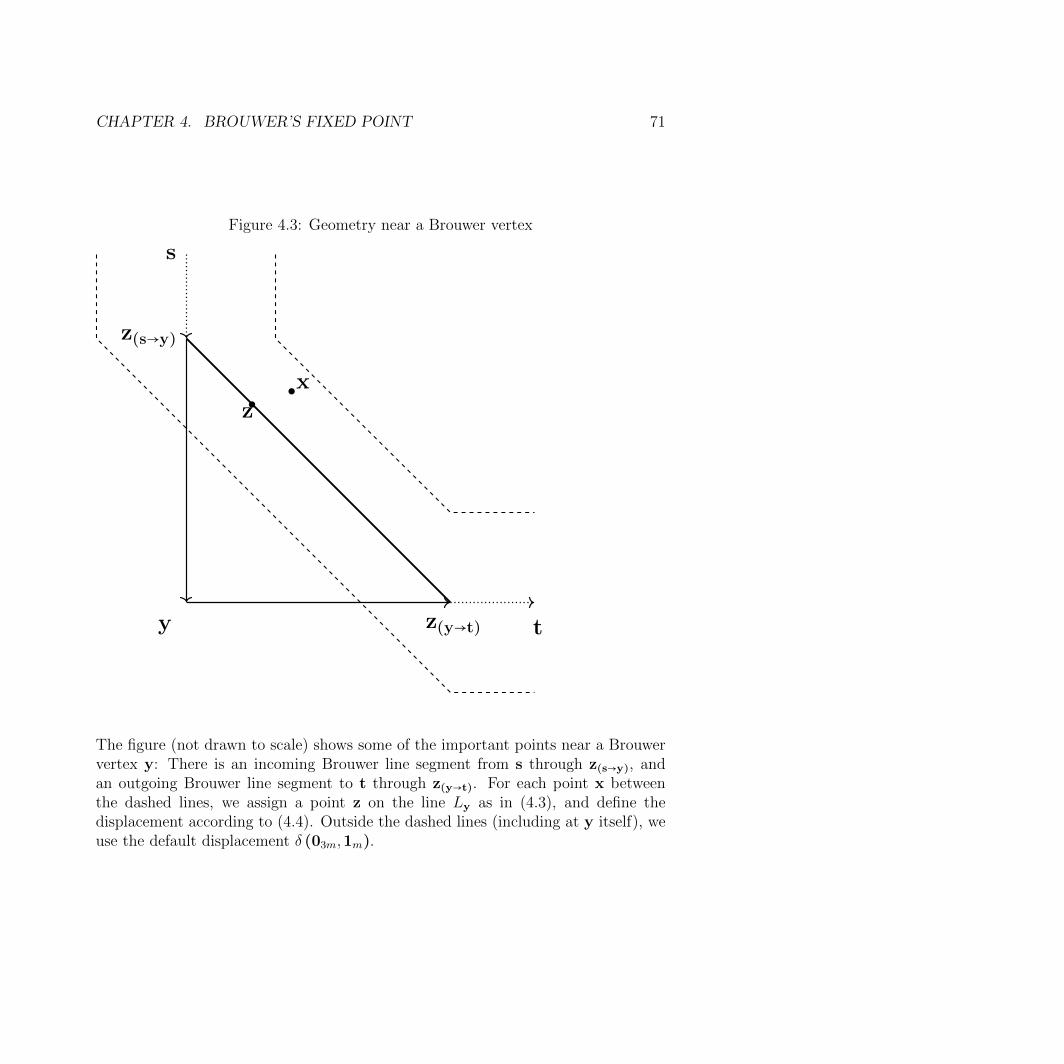
CHAPTER 4. BROUWER’S FIXED POINT 71
Figure 4.3: Geometry near a Brouwer vertex
s
z(s→y)
y z(y→t) t
x
z
The figure (not drawn to scale) shows some of the important points near a Brouwervertex y: There is an incoming Brouwer line segment from s through z(s→y), andan outgoing Brouwer line segment to t through z(y→t). For each point x betweenthe dashed lines, we assign a point z on the line Ly as in (4.3), and define thedisplacement according to (4.4). Outside the dashed lines (including at y itself), weuse the default displacement δ (03m,1m).

CHAPTER 4. BROUWER’S FIXED POINT 72
erased by the truncation. Instead, we define the displacement as follows:
g (x) ≜⎧⎪⎪⎨⎪⎪⎩
δ (03m,−1m) ∥x − z2∥2 = 0
δ (z1−x)h ∥x − z2∥2 ≥ h,
(4.8)
where z2 = (03m,2 ⋅ 1m). When θ ≜ ∑4mi=3m+1 xi ∈ (1/2,2), we interpolate between (4.7)
and (4.8) according to θ−1/23/2 .
4.2.3 Locally computing the Brouwer function
The function f defined above is local in two different ways: First, in order to computef(x) at a point x which is close to the embedding of one or a few vertices in theMembership End-of-a-Line instance I, we only need to understand I at thosevertices. The second type of locality observes that in order to compute just a singlecoordinate fi(x), we only need partial information about x.
Locality in the Membership End-of-a-Line instance
Fact 4.2.2. The function f defined below is local in the sense that there exists a classof functions fI1,I2 ∶ [−1,2]4m → [−1,2]4m which do not depend on I, and f can bedefined as an interpolation between these functions such that:
1. If the firstm-tuple of coordinates of x is 12√h-close to the encoded vertex E(v),
but the second m-tuple of coordinates of x is 12√h-far from any encoded vertex
E(w) then fI(v),I2(x) = f(x) for every I2.
2. If the second m-tuple of coordinates of x is 12√h-close to the encoded vertex
E(w), but the first m-tuple of coordinates of x is 12√h-far from any encoded
vertex E(v) then fI1,I(w)(x) = f(x) for every I1.
3. If the first m-tuple of coordinates of x is 12√h-close to the encoded vertex
E(v), and the second m-tuple of coordinates of x is 12√h-close to the encoded
vertex E(w) then fI(v),I(w)(x) = f(x).
4. If none of the above conditions are satisfied, then fI1,I2(x) = f(x) for everyI1, I2.

CHAPTER 4. BROUWER’S FIXED POINT 73
Locality in a single coordinates
In order to compute all of f (x) exactly, we essentially need to know x in everycoordinate. However, in order to compute fi (x) (the i-th coordinate of f (x)), itsuffices to know xi and that x is:
• inside the picture, but far from every Brouwer line segment;
• close to some point z on Brouwer line segment (s→ t) (but far from s and t),
– also need to know si, ti, zi, ∥x − z∥2 and ∥t − s∥2;
• close to some point z on line Ly for Brouwer vertex y on the intersection ofBrouwer lines (s→ y) and (y → t),
– also need to know si, yi, ti, zi, ∥x − z∥2 , ∥y − s∥2 , ∥t − y∥2, and α; or
• outside the picture,
– also need to know Ei∈3m+1,...,4mxi and ∥x − z∥2, where z is the (Ei∈3m+1,...,4mxi)-weighted average of z1/2 and z2.
By Lipschitz continuity, if we only want to compute fi (x) to within ±O(ε), it sufficesto know all the quantities above to within ±ε. Furthermore, at distance ±ε nearinterfaces between the different cases (inside/outside the picture, close to 0/1/2 lines),we can use the wrong displacement, and still be within ±O(ε) of fi (x).

74
Part III
PPAD

75
Chapter 5
PPAD-hardness of approximation
In this part of the dissertation we introduce and prove our PPAD-hardness of ap-proximation results, in particular for finding for Nash equilibria. As we discussed inthe introduction, for a constant number of players, we are unlikely to prove PPAD-hardness since a quasi-polynomial time approximation algorithm exists [LMM03].Our main focus in this part is games with a large number of players. For such games,there is a question of representation: the normal form representation is exponentialin the number of the players. Instead, we consider three natural and well-studiedclasses of many-player games that have succinct representations:
Definition 5.0.1. Polymatrix games In a polymatrix game [Yan68], each pair ofplayers simultaneously plays a separate two-player game. Every player has toplay the same strategy in every two-player subgame, and her utility is the sumof her subgame utilities. The game is given in the form of the payoff matrixfor each two-player game.
Graphical games In a graphical game [Kea07], the utility of each player dependsonly on the action chosen by a few other players. This game now naturallyinduces a directed graph: we say that (i, j) ∈ E if the utility of player j dependson the strategy chosen by player i. When the maximal incoming degree isbounded, the game has a representation polynomial in the number of playersand strategies.
Succinct games Most generally, in a succinct game [SV12]1 the normal form rep-resentation is succinctly described by some small circuit.
1Related notions for two-player games have been also considered by [FKS95] and [For+08].

CHAPTER 5. PPAD-HARDNESS OF APPROXIMATION 76
Any of the above restrictions suffices to guarantee that the game has a succinctrepresentation. Our main result in this part is that even for games that satisfyall restrictions simultaneously, finding an ε-approximate Nash equilibrium is PPAD-complete.
Theorem 5.0.2. There exists a constant ε > 0, such that given a degree 3, bipartite,polymatrix game where each player has two actions, finding an ε-approximate Nashequilibrium is PPAD-complete.
The notion of ε-approximate Nash equilibrium used in Theorem 5.0.2 requiresthat every player plays ε-optimally. The most interesting open question left open inthis part of the dissertation is whether the equilibrium computation problem remainsPPAD-hard even if we only require that most of the players play ε-optimally. This isthe “PCP Conjecture for PPAD”:
Conjecture 5.0.3 (PCP for PPAD). There exist constants ε, δ > 0 such that givena degree 3, bipartite, polymatrix game where each player has two actions, finding an(ε, δ)-WeakNash is PPAD-complete.
While, proving (or disproving) the “PCP Conjecture for PPAD” remains open (seeadditional discussion in Section 16.1.1), we do prove in this section that for the moregeneral class of succinct games, finding an (ε, δ)-WeakNash is indeed PPAD-hard.
Theorem 5.0.4. There exist constants ε, δ > 0, such that finding an (ε, δ)-WeakNashis PPAD-hard for succinct multiplayer games where each player has a constant num-ber of actions.
Besides Theorem 5.0.4, all our results rely in this part of the dissertation relyon the hardness of approximation for the generalized circuit problem. Generalizedcircuits are similar to standard algebraic circuits, the main difference being thatgeneralized circuits contain cycles, which allow them to verify fixed points of con-tinuous functions. A generalized circuit induces a constraint satisfaction problem,ε-Gcircuit [CDT09]: find an assignment for the values on the lines of the circuit,that simultaneously ε-approximately satisfies all the constraints imposed by the gates(see Chapter 6 for a formal definition). ε-Gcircuit was implicitly proven PPAD-complete for exponentially small ε by Daskalakis et al [DGP09], and explicitly forpolynomially small ε by Chen et al [CDT09]. Here we prove that it continues to bePPAD-complete for some constant ε.
Theorem 5.0.5 (Generalized circuit). There exists a constant ε > 0 such that ε-Gcircuit with fan-out 2 is PPAD-complete.

CHAPTER 5. PPAD-HARDNESS OF APPROXIMATION 77
This result, in turn builds on the hardness of finding an `infty-approximate fixedpoint, which we proved in Theorem 4.1.1.
We note that except for the hardness of the course allocation problem (Chap-ter 10), all the problems we consider in this part of the dissertation were previouslyknown to be PPAD-hard for polynomial approximation factors.

78
Chapter 6
The generalized circuit problem
Generalized circuits are similar to the standard algebraic circuits, the main differencebeing that generalized circuits contain cycles, which allow them to verify fixed pointsof continuous functions. We restrict the class of generalized circuits to include onlya particular list of gates described below. Formally,
Definition 6.0.1 (Generalized circuits, [CDT09]). A generalized circuit S is a pair(V,T ), where V is a set of nodes and T is a collection of gates. Every gate T ∈ Tis a 5-tuple T = G (ζ ∣ v1, v2 ∣ v), in which G ∈ Gζ ,G×ζ ,G=,G+,G−,G<,G∨,G∧,G¬ isthe type of the gate; ζ ∈ R ∪ nil is a real parameter; v1, v2 ∈ V ∪ nil are the firstand second input nodes of the gate; and v ∈ V is the output node.
The collection T of gates must satisfy the following important property: Forevery two gates T = G (ζ ∣ v1, v2 ∣ v) and T ′ = G′ (ζ ′ ∣ v′1, v′2 ∣ v′) in T , v ≠ v′.
Alternatively, we can think of each gate as a constraint on the values on the in-coming and outgoing wires. We are interested in the following constraint satisfactionproblem: given a generalized circuit, find an assignment to all the wires that simul-taneously satisfies all the gates. When every gate computes a continuous functionof the incoming wires (with inputs and output in [0,1]), a solution must exist byBrouwer’s fixed point theorem.
In particular, we are interested in the approximate version of this CSP, where wemust approximately satisfy every constraint.
Definition 6.0.2. Given a generalized circuit S = (V,T ), we say that an assignmentx∶V → [0,1] ε-approximately satisfies S if for each of the following gates, x satisfiesthe corresponding constraints:

CHAPTER 6. THE GENERALIZED CIRCUIT PROBLEM 79
Gate Constraint
Gζ (α ∣∣ a) x [a] = α ± εG×ζ (α ∣ a ∣ b) x [b] = α ⋅ x [a] ± εG= (∣ a ∣ b) x [b] = x [a] ± εG+ (∣ a, b ∣ c) x [c] = min (x [a] + x [b] ,1) ± εG− (∣ a, b ∣ c) x [c] = max (x [a] − x [b] ,0) ± ε
G< (∣ a, b ∣ c) x [c] =⎧⎪⎪⎨⎪⎪⎩
1 ± ε x [a] < x [b] − ε0 ± ε x [a] > x [b] + ε
G∨ (∣ a, b ∣ c) x [c] =⎧⎪⎪⎨⎪⎪⎩
1 ± ε x [a] = 1 ± ε or x [b] = 1 ± ε0 ± ε x [a] = 0 ± ε and x [b] = 0 ± ε
G∧ (∣ a, b ∣ c) x [c] =⎧⎪⎪⎨⎪⎪⎩
1 ± ε x [a] = 1 ± ε and x [b] = 1 ± ε0 ± ε x [a] = 0 ± ε or x [b] = 0 ± ε
G¬ (∣ a ∣ b) x [b] =⎧⎪⎪⎨⎪⎪⎩
1 ± ε x [a] = 0 ± ε0 ± ε x [a] = 1 ± ε
(Where Gζ and G×ζ also take a parameter α ∈ [0,1].)
Given a generalized circuit S = (V,T ), ε-Gcircuit is the problem of finding anassignment that ε-approximately satisfies it.
Brittle comparators Intuitively, in order for (approximate) solutions to the cir-cuit problem to correspond to (approximate) equilibria, all our gates should imple-ment continuous (Lipschitz) functions. The gate G< (∣ a, b ∣ c), for example, approx-
imates that the function c (a, b) =⎧⎪⎪⎨⎪⎪⎩
1 a < b0 a ≥ b
, which is not continuous. To overcome
this problem, Daskalakis et al [DGP09] defined the brittle comparator: when a is (ε-)larger than b, it outputs 0; when b is (ε-) larger than a, it outputs 1. However, whena and b are (ε-approximately) equal, its behavior is undefined.
Brittleness introduces difficulties in the transition from continuous to discretesolutions. This challenge is overcome by an averaging gadget, which is described indetail in Section 6.2.
Our results
ε-Gcircuit was implicitly proven PPAD-complete for exponentially small ε by Daskalakiset al [DGP09], and explicitly for polynomially small ε by Chen et al [CDT09]. Here

CHAPTER 6. THE GENERALIZED CIRCUIT PROBLEM 80
we prove that it continues to be PPAD-complete for some constant ε.
Theorem (Generalized circuit; Theorem 5.0.5 restated). There exists a constantε > 0 such that ε-Gcircuit with fan-out 2 is PPAD-complete.
6.1 Proof overview
The key idea that enables us to improve over previous hardness of approximationfor ε−Gcircuit (and Nash equilibrium) [DGP09; CDT09] is our particular choiceof hard fixed point instance in Section 4.1. The first advantage is that our instanceis simply harder to approximate: finding an ε-approximate fixed point (i.e. x suchthat ∥f (x) − x∥∞ ≤ ε) is PPAD-hard for ε = Ω (1) (as opposed to ε = 1/ exp (n) for[DGP09] and ε = 1/poly (n) in [CDT09]).
A simpler averaging gadget Our construction of hard instances of Brouwer func-tions, as do the ones form previous works, partitions the (continuous) hypercube intosubcubes, and define the function separately on each subcube. When we constructa circuit that approximately simulates such a Brouwer function, we have a problemnear the facets of the subcubes: using approximate gates and brittle comparators(both defined formally in Chapter 6), one cannot determine to which subcube theinput belongs. This is the most challenging part of our reduction, as was also thecase in [DGP09; CDT09].
Originally, Daskalakis et al [DGP09] tackled this obstacle by approximating f (x)as the average over a ball around x. The key observation is that even if x is close toa facet between subcubes, most of the points in its neighborhoods will be sufficientlyfar. Yet if f is Lipschitz they are mapped approximately to the same point asx. This works fine in O (1) dimensions, but then the inapproximability parameteris inherently exponentially small (in constant dimensions, it is easy to construct a1/poly (n)-net over the unit hypercube). For poly (n) dimensions, the (discretizationof the) ball around x contains exponentially many points.
Chen et al [CDT09] overcome this problem using equiangle sampling: considermany translations of the input vector by adding small multiples of the all-ones vector;compute the displacement for each translation, and average. Since each translationmay be close to a facet in a different dimension, Chen et al consider a polynomialnumber of translations. Thus, all translations must be polynomially close to eachother - otherwise they will be too far to approximate the true input.
We avoid this problem by observing another nice property of the [HPV89]’s con-struction: when the input vector lies near two or more facets, the displacement is

CHAPTER 6. THE GENERALIZED CIRCUIT PROBLEM 81
Figure 6.1: Comparison of averaging gadgets
x
Daskalakis et al [DGP09]
x
Chen et al [CDT09]
x
This paper
A comparison of the averaging gadgets of [DGP09], [CDT09], and this paper. x is thepoint whose displacement we would like to estimate using imprecise gates and brittlecomparators. Points that are too close to a facet between subcubes are denoted bytriangles, while points that are sufficiently far are denoted by circles. Finally, in thispaper we have a “safe” zone (shaded) around the corner where we don’t need toparse the subcube; thus we only need to avoid one facet.
(approximately) the same, regardless of the subcube. Once we rule out such points,it suffices to sample only a constant number of points (as at most one of them maybe too close to a facet). See also illustration in Figure 6.1.
Completing the proof Given a point x′ ≈ x which is safely in the interior of one
subcube, we can parse the corresponding binary vector, use logical operator gates tosimulate the End-of-a-Line circuit, and then approximately compute f (x′). Thisis tedious, but mostly straightforward.
One particular challenge that nevertheless arises is preventing the error fromaccumulating when concatenating approximate gates. Of course this is more difficultin our setting where each gate may err by a constant ε > 0. Fortunately, the definitionof ε-Gcircuit provides logical operator gates that round the output to 0,1 beforeintroducing new error. As long as the inputs are unambiguous bits, approximatelogical operator gates can be concatenated without accumulating errors.
In order to carry out the reduction to Nash equilibrium (Section 7.1), we mustfirst ensure that every gate in our generalized circuit has a constant fan-out (Section6.3). We can replace each logical operator gate with a binary tree of fan-out 2,

CHAPTER 6. THE GENERALIZED CIRCUIT PROBLEM 82
alternating negation gates (that do not accumulate error). Given an arithmetic gatewith large fan-out, we convert its output to unary representation1 using a constantnumber of (fan-out 2) gates. Then we copy the unary representation using a binarytree of negation gates. Finally, we convert each copy back to a real number using aconstant number of gates.
6.2 From Brouwer to ε-Gcircuit
In this section we prove a slightly easier version of Theorem 5.0.5, for a generalizedcircuit with unbounded fan-out. We reduce to constant fan-out in the next section.
Proposition 6.2.1. There exists a constant ε > 0 such that ε-Gcircuit is PPAD-complete.
Proof. We continue to denote the hard Brouwer function by f ∶ [0,1]2n+2 → [0,1]2n+2,
and its associated displacement by g (y) = f (y)−y. We design a generalized circuitS that computes f , and verifies that the output is equal to the input. We showthat every ε-approximate solution to S corresponds to an O (ε1/4)-approximate fixedpoint of f .
Recall that the construction from Section (4.1) divides the hypercube into equal-sized subcubes (of length 1/4). Furthermore, all the paths in H are embedded inthe 22n+1 subcubes that belong to the picture. For ease of exposition, we presenta construction that only works for points in the picture, i.e. y ∈ [1/4,3/4]2n+1 ×[1/4,1/2]. It is straightforward how to use the same ideas to extend the circuit todeal with all y ∈ [0,1]2n+2
.The most challenging part of the construction is the extraction of the information
about the local subcube: is it part of a tube? if so, which are the entrance and exitfacets? This is done by extracting the binary representation of the current subcube,and feeding it to the (Boolean) circuit that computesH (recall thatH is our collectionof paths and cycles from Section (4.1.2)). Notice that whenever we have valid logicbits, i.e. x [b] < ε or x [b] > 1 − ε, we can perform logic operations on them withoutincreasing the error.
Once we know the behavior of the path on the current subcube, we simply have tolocally implement the mapping from the previous section, for which we have a closedform description, using the available gates in the definition of generalized circuits.
1Unary representation of numbers with constant precision is prevalent throughout our imple-mentation of the generalized circuit. We prefer unary representation over binary, because in theformer at most one bit can be ambiguous due to the use of brittle comparators.

CHAPTER 6. THE GENERALIZED CIRCUIT PROBLEM 83
Since this definition does not include multiplication and division, we implement mul-tiplication and division in Algorithms 2 and 3 in Subsection 6.2.1.
Our construction has four parts: (1) equiangle sampling segment, (2) computingthe displacement, (3) summing the displacement vectors, and (4) closing the loop.The first part contains a new idea introduced in this paper: using a constant sizesample. The second part is a more technical but straightforward description of theimplementation of the closed-form mapping by approximate gates. The third andfourth parts are essentially identical to [CDT09].
6.2.1 Subroutines
In this subsection we show how to implement a few useful subroutines using the gatesin the definition of ε-Gcircuit.
6.2.1.1 If-Else
We begin by describing how to implement a simple if-else. Similar ideas can be usedto implement more involved cases such as (4.1).
Claim 6.2.2. In any ε-approximate solution to If-Else(∣ a, b, c ∣ d),
x [d] =⎧⎪⎪⎨⎪⎪⎩
x [c] ±O (ε) if x [a] < √ε
x [b] ±O (ε) if x [a] > 1 −√ε.
Proof. By definition of G¬, we have that
x [a] =⎧⎪⎪⎨⎪⎪⎩
1 ± ε if x [a] < √ε
0 ± ε if x [a] > 1 −√ε.
Algorithm 1 If-Else(∣ a, b, c ∣ d)1. G¬ (∣ a ∣ a)# a is the negation of a
2. G− (∣ b, a ∣ b′)# b′ is (approximately) equal to b iff a = 1
3. G¬ (∣ a ∣ a)# a is the roudning of a to 0,1
4. G− (∣ c, a ∣ c′)# c′ is (approximately) equal to c iff a = 0
5. G− (∣ b′, c′ ∣ d)

CHAPTER 6. THE GENERALIZED CIRCUIT PROBLEM 84
Therefore by definition of G−,
x [b′] =⎧⎪⎪⎨⎪⎪⎩
0 ±O (ε) if x [a] < √ε
x [b] ±O (ε) if x [a] > 1 −√ε.
Similarly,
x [c′] =⎧⎪⎪⎨⎪⎪⎩
x [c] ±O (ε) if x [a] < √ε
0 ±O (ε) if x [a] > 1 −√ε.
Finally, the claim follows by definition of G+.
6.2.1.2 Multiply
Claim 6.2.3. In any ε-approximate solution to Multiply(∣ a, b ∣ c),
x [c] = x [a] ⋅ x [b] ±O (√ε) .
Proof. For any k, the first gate implies that
x [ζk] = k√ε ± ε.
The second gate thus gives
x [ak] =⎧⎪⎪⎨⎪⎪⎩
0 ± ε if x [a] > k√ε +O (ε)1 ± ε if x [a] < k√ε −O (ε) .
(6.1)
Notice that the above equation is ambiguous for at most one value of k. In particular,
∑k
(1 − x [ak])√ε = x [a] ±O (
√ε) . (6.2)
We also havex [dk] = x [b] ⋅
√ε ± ε.
The subtraction gate zeros x [dk] for all k such that x [a] < k√ε − O (ε), and hasnegligible effect for k such that x [a] > k√ε +O (ε):
x [ek] =⎧⎪⎪⎨⎪⎪⎩
x [b] ⋅√ε ± 2ε if x [a] > k√ε +O (ε)0 ± 2ε if x [a] < k√ε −O (ε) .
The sum of the x [ek]’s satisfies:
∑k
x [ek] = x [a] ⋅ x [b] ±O (√ε) ,

CHAPTER 6. THE GENERALIZED CIRCUIT PROBLEM 85
Algorithm 2 Multiply(∣ a, b ∣ c)1. Gζ (0 ∣∣ h0)
2. for each k ∈ [1/√ε]:
a) Gζ (k√ε ∣∣ ζk), G< (∣ a, ζk ∣ ak)
# The vector (ak) is the unary representation of a
∑k∶x[ak]<ε
√ε = max
k∶x[ak]<εk√ε = x [a] ±O (
√ε)
b) G×ζ (√ε ∣ b ∣ dk)
# The vector (dk) is simply equal to b ⋅√ε everywhere.
∑k∶x[ak]<ε
x [dk] =⎛⎝ ∑k∶x[ak]<1−ε
√ε⎞⎠⋅ x [b] ±O (
√ε) = x [a] ⋅ x [b] ±O (
√ε)
c) G− (∣ dk, ak ∣ ek)# The vector (ek) is b ⋅√ε only when (ak) < ε.
∑k∶x[ak]<ε
x [ek] = x [a] ⋅ x [b] ±O (√ε)
d) G+ (∣ hk−1, ek ∣ hk)# Finally, we sum the ek’s to get a ⋅ b
x [h1/√ε] = x [a] ⋅ x [b] ±O (√ε)
3. G= (∣ h1/√ε ∣ c)

CHAPTER 6. THE GENERALIZED CIRCUIT PROBLEM 86
where we have an error of ±O (√ε) arising from aggregating ±2ε for 1/√ε distinct
k’s, and another ±O (√ε) from (6.2).By induction, each hk is approximately equal to the sum of the first x [ej]’s:
x [hk] =k
∑j=1
x [ej] ± kε.
In particular, we have
x [h1/√ε] = ∑k
x [ek] ±√ε
= x [a] ⋅ x [b] ±O (√ε) .
6.2.1.3 Divide
Claim 6.2.4. In any ε-approximate solution to Divide(∣ a, b ∣ c),x [c] ⋅ x [b] = x [a] ±O (
√ε) .
Notice that for Algorithm 3, in any ε-approximate solution, x [c] = x [a] /x [b] ±O (√ε) /x [b]; when x [b] and ε are bounded away from 0, this is only a constantfactor increase in the error.
Proof. For each k, we have
x [bk] = k√ε ⋅ x [b] ± ε.
Thus also
x [dk] =⎧⎪⎪⎨⎪⎪⎩
1 ± ε if x [a] > k√ε ⋅ x [b] +O (ε)0 ± ε if x [a] < k√ε ⋅ x [b] −O (ε) .
Notice that x [dk] is ambiguous for at most k. Furthermore, aggregating the ±ε errorover 1/√ε distinct k’s, we have:
∑x [dk] ⋅√εx [b] = x [a] ±O (
√ε) .
x [ek]’s are a step closer to what we need:
x [ek] = x [dk]√ε ± ε,
and therefore also
∑x [ek] ⋅ x [b] = x [a] ±O (√ε) . (6.3)
Finally, by inductionx [h1/√ε] =∑x [ek] ±
√ε,
and the claim follows by plugging into (6.3).

CHAPTER 6. THE GENERALIZED CIRCUIT PROBLEM 87
Algorithm 3 Divide(∣ a, b ∣ c)1. Gζ (0 ∣∣ h0)
2. for each k ∈ [1/√ε]:
a) G×ζ (k√ε ∣ b ∣ bk), G< (∣ bk, a ∣ dk)
# The vector (dk) is the unary representation of a/b
⎛⎝ ∑k∶x[dk]>ε
√ε⎞⎠⋅ x [b] = ( max
k∶x[dk]>εk√ε) ⋅ x [b] = x [a] ±O (
√ε)
b) G×ζ (√ε ∣ dk ∣ ek)
# The vector (ek) is a (√ε)-scaled version of (dk)
(∑x [ek]) ⋅ x [b] = x [a] ±O (√ε)
c) G+ (∣ hk−1, ek ∣ hk)# Finally, we sum the ek’s
x [h1/√ε] ⋅ x [b] = x [a] ±O (√ε)
3. G= (∣ h1/√ε ∣ c)

CHAPTER 6. THE GENERALIZED CIRCUIT PROBLEM 88
6.2.1.4 Max

CHAPTER 6. THE GENERALIZED CIRCUIT PROBLEM 89
Claim 6.2.5. In any ε-approximate solution to Max(∣ a1, . . . an ∣ b),
x [b] = maxx [ai] ±O (√ε) .
Proof. Similarly to (6.1), we have that for each i, k
x [ck,i] =⎧⎪⎪⎨⎪⎪⎩
0 ± ε if x [ai] < k√ε −O (ε)
1 ± ε if x [ai] > k√ε +O (ε) .
For each k, taking OR of all the ck,i’s gives (approximately) 1 iff any of the x [ai]’sis sufficiently large; in particular if the maximum is:
x [dk,n] =⎧⎪⎪⎨⎪⎪⎩
0 ± ε if maxi x [ai] < k√ε −O (ε)
1 ± ε if maxi x [ai] > k√ε +O (ε) .
Therefore also (similarly to (6.2)),
∑k
x [dk,n]√ε = max
ix [ai] ±O (
√ε) .
The x [ek] take care of scaling by√ε:
∑k
x [ek] = maxi
x [ai] ±O (√ε) .
Finally, by induction,
x [h1/√ε] = maxx [ai] ±O (√ε) .
6.2.1.5 Interpolate

CHAPTER 6. THE GENERALIZED CIRCUIT PROBLEM 90
Algorithm 4 Max(∣ a1, . . . an ∣ b)1. Gζ (0 ∣∣ h0)
2. for each k ∈ [1/√ε]:
a) Gζ (k√ε ∣∣ ζk)
b) Gζ (0 ∣∣ dk,0)c) for each i ∈ [n]:
i. G< (∣ ζk, ai ∣ ck,i)# The vector (ck,i)k is the unary representation of ai:
∀i ( maxk∶x[ck,i]>ε
k√ε) = x [ai] ±O (
√ε)
ii. G∨ (∣ dk,i−1, ck,i ∣ dk,i)# The vector (dk,n) is the unary representation of maxai:
( maxk∶x[dk,n]>ε
k√ε) = maxx [ai] ±O (
√ε)
d) G×ζ (√ε ∣ dk,n ∣ ek)
# The vector (ek) is a (√ε)-scaled version of (dk)
(∑x [ek]) = maxx [ai] ±O (√ε)
e) G+ (∣ hk−1, ek ∣ hk)# Finally, we sum the ek’s
x [h1/√ε] = maxx [ai] ±O (√ε)
3. G= (∣ h1/√ε ∣ b)

CHAPTER 6. THE GENERALIZED CIRCUIT PROBLEM 91
Claim 6.2.6. In any ε-approximate solution to Interpolate(a,wa, b,wb ∣ c),
x [c] (x [wa] + x [wb]) = (x [wa] ⋅ x [a] + x [wb] ⋅ x [b]) ±O (√ε) .
Proof. By Claim 6.2.4, we have
x [wa] ⋅ (x [wa] + x [wb]) = x [wa] ±O (√ε)
x [wb] ⋅ (x [wa] + x [wb]) = x [wb] ±O (√ε) .
Therefore, by Claim 6.2.3,
x [ca] ⋅ (x [wa] + x [wb]) = x [wa] ⋅ x [c] ±O (√ε)
x [cb] ⋅ (x [wa] + x [wb]) = x [wb] ⋅ x [c] ±O (√ε) .
The claim follows by definition of G+.

CHAPTER 6. THE GENERALIZED CIRCUIT PROBLEM 92
Algorithm 5 Interpolate(a,wa, b,wb ∣ c)
1. G×ζ (1/2 ∣ wa ∣ wa/2) and G×ζ (1/2 ∣ wb ∣ wb/2)# We divide by 2 before adding in order to stay in [0,1]
2. G+ (∣ wa/2,wb/2 ∣ wa/2+b/2) Add the weights
3. Divide(∣ wa/2,wa/2+b/2 ∣ wa) and Divide(∣ wb/2,wa/2+b/2 ∣ wb),
# wa and wb are the normalized weights:
x [wa] ⋅ (x [wa] + x [wb]) = x [wa] ±O (√ε)
4. Multiply(∣ wa, a ∣ ca) and Multiply(∣ wb, b ∣ cb)# ca and cb are the a and b components, respectively, of c:
x [ca] = x [wa] ⋅ x [a] / (x [wa] + x [wb]) ±O (√ε) / (x [wa] + x [wb])
5. G+ (∣ ca, cb ∣ c)
# Finally, c is the interpolation of a and b:
x [c] = (x [wa] ⋅ x [a] + x [wb] ⋅ x [b]) / (x [wa] + x [wb])±O (
√ε) / (x [wa] + x [wb])

CHAPTER 6. THE GENERALIZED CIRCUIT PROBLEM 93
6.2.2 Equiangle sampling segment
The first information we require in order to compute the Hirsch et al mapping f (y)is about the subcube to which y belongs: is it part of the tube? if so, which are theentrance and exit facets? In order to answer those questions, we extract the binaryrepresentation of the cube. Recall that our circuit uses brittle comparators; thuswhen y is close to a facet between subcubes, the behavior of the brittle comparatorsmay be unpredictable. We start with the easy case, where y is actually far fromevery facet:
Definition 6.2.7. We say that y is an interior point if for every i, ∣yi − 1/2∣ > ε;otherwise, we say that y is a boundary point.
A very nice property of the Hirsch et al construction is that whenever y is atthe intersection of two or more facets, the displacement is the same: g (y) = δξ2n+2.Thus, by the Lipschitz property of g, whenever y is close to the intersection of twoor more facets, the displacement is approximately δξ2n+2. For such y’s, we don’t careto which subcube they belong.
Definition 6.2.8. We say that y is a corner point if there exist distinct i, j ∈ [2n + 2]such that ∣yi − 1/2∣ < ε1/4 and ∣yj − 1/2∣ < ε1/4.
(Notice that y may be an interior point and a corner point at the same time.)We still have a hard time handling y’s which are neither an interior point nor
a corner point. To mitigate the effect of such y’s we use an equiangle averagingscheme. Namely we consider the set:
Eε (y) = yl = y + (6l ⋅ ε)1∶0 ≤ l < 1/√ε
where 1 denotes the all-ones vector. Notice that since g is λ-Lipschitz for constantλ, g (yl) will be approximately the same for all yl ∈ Eε (y).Fact 6.2.9. If any yl ∈ Eε (y) is not a corner point, then at most one yl
′ ∈ Eε (y) isa boundary point.
Proof. For each dimension, at most one element in Eε (y) can be ε-close to the (1/2)facet. Thus if two elements in Eε (y) are boundary points, it must be because ofdistinct dimensions - and therefore every yl is a corner point.
Given input y, we compute the displacement g (⋅) separately and in parallel foreach yl ∈ Eε, and average at the end. Since at most one yl is a boundary point, thiswill incur an error of at most
√ε.

CHAPTER 6. THE GENERALIZED CIRCUIT PROBLEM 94
In the generalized circuit we can construct Eε using (1/√ε) auxiliary nodes andGζ and G+ gates:
x [yli] = minx [y0i ] + (6l ⋅ ε) ,1 ± 2ε
6.2.3 Computing the displacement
For each yl ∈ Eε, we construct a disjoint circuit that approximates the displacementg (yl). In the description of the circuit below we omit the index l.
Lemma 6.2.10. The circuit below O (√ε)-approximately simulates the computationof the Hirsch et al displacement:
1. Whenever (x [yi])i∈[2n+2] is an interior point,
x [g+i ] − x [g−i ] = gi (x [y]) ±O (ε1/4)
2. Furthermore, whenever (x [yi])i∈[2n+2] is a corner point,
x [g+2n+2] − x [g−2n+2] = δ ±O (√ε)
and ∀i < 2n + 2:x [g+i ] − x [g−i ] = 0 ±O (
√ε)
Proof. We construct the circuit in five stages: (1) given y, we extract b, that is thebinary representation of the corresponding subcube in 0,12n+2
; (2) we then computewhether b belongs to a path in H, and if so which are the previous and next vertices;(3) we compute the centers of the coordinate systems corresponding to the entranceand exit facets, and label them zin and zout; (4) we project y to each facet, andtransform this projection to the local polar coordinate systems - (rin,pin); and (5)finally, we use all the information above to compute the displacement g = g (y).
The correctness of Lemma 6.2.10 follows from Claims 6.2.11-6.2.17.
Extract b ∈ 0,12n+2
Our first step is to extract the binary vector b which represents the subcube to whichy belongs. In other words we want bi to be the indicator of yi < 1/2. We do thatby adding the following gadgets: Gζ (1/2 ∣∣ c1/2) and, for each i, G< (∣ yi, c1/2 ∣ bi).Observe that now
x [bi] =⎧⎪⎪⎨⎪⎪⎩
0 ± ε x [yi] < x [c1/2] − ε1 ± ε x [yi] > x [c1/2] + ε
Claim 6.2.11. If x [y] is an interior point, x [b] is the correct representation (up toε error) of the corresponding bits in 0,12n+2
.

CHAPTER 6. THE GENERALIZED CIRCUIT PROBLEM 95
Neighbors in H
Given x [b] we can construct, using G∧’s and G¬’s and a polynomial number ofunused nodes, the circuits SH and PH that give the next and previous vertex visitedby our collection of paths, H. The output of each circuit is represented by 2n + 2unused nodes PH
i (b) and SHi (b).
Recall that H is defined in 0,12n+1, so the last input bit is simply ignored (inside
the picture it is always 0); the last output bit is used as follows. Our conventionis that starting points and end points correspond to PH (b) = b and SH (b) = b,respectively, and likewise for points that do not belong to any path. An exception tothis is the 0 starting point, which will correspond to PH (0) = (02n+1; 1): This is inaccordance with the Hirsch et al construction, where the home subcube is constructedas if it continues a path from the subcube above it.
Claim 6.2.12. If x [b] is an ε-approximate binary vector, i.e. x [b] ∈ ([0, ε] ∪ [1 − ε,1])2n+2,
then x [PH (b)] and x [SH (b)] correctly represent (up to ε error) the previous vertexand next vertex in H.
Entrance and exit facets
Let b+ini = bi ∧ ¬PHi (b), i.e. b+ini is 1 if the path enters the current subcube via the
positive i-th direction; define b−ini analogously. Let bini denote the OR of b+ini andb−ini .
The center of the entrance facet is constructed via Gζ , G×ζ , G+, and G− accordingto the formula:
zini =⎧⎪⎪⎪⎪⎨⎪⎪⎪⎪⎩
1/2 − h/2 bini = 0 AND bi = 0
1/2 + h/2 bini = 0 AND bi = 1
1/2 bini = 1
Construct zout analogously.Notice that if we know on which coordinate the path enters, in 0,12n+2
it hasonly one possible direction; in the Hirsch et al hypercube this corresponds to alwaysentering from the center (i.e. from the yi = 1/2 facet). Also, if b corresponds to anon-trivial starting point bin = 0 and zin is simply the center of the subcube (andsimilarly for bout,zout when b is an end point).
Claim 6.2.13. If x [b], x [PH (b)], and x [SH (b)] are ε-approximate binary vectors,then x [zin] and x [zout] are O (ε)-approximations to the centers of the entrance facetand exit facets, respectively.

CHAPTER 6. THE GENERALIZED CIRCUIT PROBLEM 96
Max-norm polar coordinates
We are now ready to compute the local max-norm polar coordinates of the projectionsof y on the entrance and exit facets.
The max-norm radius is given by
rin = maxi∶bini =0
∣zini − yi∣
Finding the maximum of a (length 2n+1) vector requires some care when on eachgate we can incur a constant error, the details are described in Algorithm 4.
The direction (max-norm) unit-vector, p, is given by
pini = (zini − yi) /rin
Division is computed using Divide, introducing an error of O (√ε/rin); this approx-imation suffices because for rin < h/8, we multiply pini by rin when we interpolate.Also, we will use two nodes for each pini to represent the positive and negative values.We do the same for (rout,pout).Claim 6.2.14. If x [y] is an interior point, then x [rin] and x [rout] are O (√ε)-approximations to the distances of x [y] from x [zin] and x [zout], respectively. Fur-thermore, x [pin] and x [pout] are O (√ε/x [rin])- and O (√ε/x [rout])- to the unit-length vectors that point from x [y] in the directions of x [zin] and x [zout], respec-tively.
The final displacement
Given pin and bin, we can compute gin for the special values of rin. Recall that
gin (⟨rin,pin⟩) =
⎧⎪⎪⎪⎪⎪⎪⎪⎨⎪⎪⎪⎪⎪⎪⎪⎩
δ (b+in − b−in) rin = 0
−δpin rin = h/8δ (b−in − b+in) rin = h/4δξ2n+2 rin = h/2
We use Algorithm 5 to interpolate for intermediate values of rin. We also needto interpolate between gin and gout. The ratio at which we interpolate is exactlythe ratio between the distance of y from the entrance and exit facets. We label thepositive and negative components of this last interpolation g(interior)+ and g(interior)−,respectively.
When y is close to both facets, the interpolation may be inaccurate; however,in this case it is a corner point. (We remark that this seems to be the only part

CHAPTER 6. THE GENERALIZED CIRCUIT PROBLEM 97
of the proof which requires us to set the threshold for a corner point and the finalerror at Θ (ε1/4) rather than Θ (√ε); this issue may be avoidable by a more carefulconstruction of Algorithms 3 and 5.)
Claim 6.2.15. If x [y] is an interior point of an intermediate subcube in the tube, andit is not a corner point, then (x [g(interior)+] − x [g(interior)−]) is aO (ε1/4)-approximationof the Hirsch et al displacement g (x [y]).
Corner points We must ensure that if y is a corner point, we set g(corner)+ = δξ2n+2
and g(corner)− = 0: check over all pairs of coordinates whether ∣x [yi] − 1/2∣ < 2ε1/4
and ∣x [yj] − 1/2∣ < 2ε1/4. Let z be the variable representing the OR of those (2n+22
)indicators. Interpolate (e.g. using Algorithm 5) between the (g(interior)+,g(interior)−)we computed earlier and δξ2n+2 with weights z and ¬z. Label the result of theinterpolation (g(tube)+,g(tube)−).
We remark that whenever z is ambiguous, i.e. the second smallest ∣x [yi] − 1/2∣is very close to 2ε1/4, then we cannot predict the value of x [z]; it can take any valuein [0,1]. Nevertheless, in this case x [y] is not a corner point, thus for most yl ∈ Eε,x [yl] is an interior point. This means that by Claim 6.2.15, we would compute the(approximately) correct interior displacement (x [g(interior)+] − x [g(interior)−]). Sincex [y] is close to a corner point, this value is very close to δξ2n+2 = (x [g(corner)+] − x [g(corner)−]).Therefore, although we don’t know the value of x [z], we use it to interpolate betweentwo (approximately) equal vectors - so the result is guaranteed to be (approximately)correct regardless of the value of x [z].Claim 6.2.16. If x [y] is a corner point, then (x [g(tube)+] − x [g(tube)−]) is a O (√ε)-approximation of δξ2n+2, and thus also a O (ε1/4)-approximation of the Hirsch et aldisplacement g (x [y]). Furthermore, Claim 6.2.15 continues to hold for (g(tube)+,g(tube)−).
Start/end subcubes and subcubes outside the tube For start/end subcubes(except the home subcube) we use a slightly different (Cartesian) interpolation thatyields a fixed point in the center of the subcube, and a displacement of δξ2n+2 onall facets but the exit/entrance facet, respectively. For subcubes in the picture butoutside the tube, we again set g = δξ2n+2.
Notice that we can infer the type of subcube from the following two-bits vector:
T = (∨ibini ,∨ibouti )
If T = (0,0), the subcube is outside the tube; when T = (0,1), we are at a startsubcube, while T = (1,0) corresponds to an end subcube; T = (1,1) is an intermediatesubcube in the tube. Finally, interpolate between the displacement for each type ofsubcube using T and ¬T ; label the result of the interpolation (g+,g−).

CHAPTER 6. THE GENERALIZED CIRCUIT PROBLEM 98
Claim 6.2.17. If x [y] is either an interior point or a corner point, of any subcubein the slice, then (x [g+] − x [g−]) is an O (ε1/4)-approximation of the Hirsch et aldisplacement g (x [y]).
6.2.4 Summing the displacement vectors
We are now ready to average over the displacement vectors we computed for eachyl. Using G×ζ and G+ we have that
x [g+i ] =1/√ε∑l=1
(√εx [gl+i ]) ±O (
√ε) and x [g−i ] =
1/√ε∑l=1
(√εx [gl−i ]) ±O (
√ε)
Lemma 6.2.18. For every input x [y] and every i ∈ [2n + 2],
x [g+i ] − x [g−i ] = gi (x [y]) ±O (ε1/4)
Proof. By Fact 6.2.9, every yl ∈ Eε, except at most one, is either an interior point or acorner point. By Lemma 6.2.10, for all those yl, (x [g+li ] − x [g−li ]) is at most O (ε1/4)-far from the right displacement. The single point which is neither an interior pointnor a corner point increases the error by at most O (√ε), as does the summationabove. Finally, because g is λ-Lipschitz for constant λ, the error added due to thedistance between the yl’s is again at most O (√ε).
6.2.5 Closing the loop
Finally, for each i ∈ [2n + 2]: G+ (∣ y1i , g
+i ∣ y′i), G+ (∣ y′i, g−i ∣ y′′i ) and G= (∣ y′′i ∣ y1
i ).
6.3 Gcrcuit with Fan-out 2
In the previous section, we proved that ε-Gcircuit is PPAD-complete for some con-stant ε > 0. Each generalized circuit gate has fan-in at most 2, which would eventuallycorrespond to a bound on the incoming degree of each player in the graphical game.In order to bound the total degree (as well as for the application to A-CEEI), weneed to also bound fan-out of each gate.
Proof of Theorem 5.0.5. We present a black-box reduction that converts a generalε′-Gcircuit instance to an instance of ε-Gcircuit with fan-out 2, for ε′ = Θ (√ε).Daskalakis et al [DGP09] bound the fan-out of the generalized circuit by introducing

CHAPTER 6. THE GENERALIZED CIRCUIT PROBLEM 99
Algorithm 6 Real2Unary(∣ a ∣ b1, . . . b4/ε′)
1. G= (∣ a ∣ c0)
2. for each k ∈ [4/ε′]:
a) G= (∣ ck−1 ∣ ck)# The ck’s are simply copies of a, ensuring that each gate has fan-out atmost 2:
∀k x [ck] = x [a] ± (k + 1) ε
b) Gζ (kε′/4 ∣∣ ζk)c) G< (∣ ζk, ck ∣ bk)
# The vector (bk) is the unary representation of a:
∀i ( maxk∶x[bk]>ε
kε′/4) = x [a] ± ε′/2
a binary tree of G= gates. Unfortunately, this blows up the error: each G= gateintroduces an additive error of ε, so the increase is proportional to the depth ofthe tree, i.e. Θ (ε ⋅ logn). While this was acceptable for [DGP09] who used anexponentially small ε, it clearly fails in our setting.
We overcome this obstacle by resorting to logical gates (G<, G∨, G∧, and inparticular G¬). Recall that the logical gates are at most ε′-far from the correctBoolean value. Therefore, concatenating multiple logical gates does not amplify theerror. In particular, if any logical gate has a large fan-out, we can distribute itsoutput using a binary tree of G¬ gates (we use trees of even depth). When the gateis arithmetic (Gζ , G×ζ , G=, G+, or G−), we convert its output to unary representationover Θ (ε′) logical gates (Algorithm 6). Then, we copy the unary representation usingtrees of G¬ gates. Finally, we use G×ζ and G+ gates to convert each copy of the unaryrepresentation back to a real value in [0,1] (Algorithm 7).
It is interesting to note that for constant ε and ε′, the unary representation hasconstant size, so the number of new gates is proportional to the original fan-out (i.e.the number of leaves of the binary tree that copies the unary representation). Inparticular this reduction increases the size of the circuit by a factor of Θ (1/ε′).

CHAPTER 6. THE GENERALIZED CIRCUIT PROBLEM 100
Algorithm 7 Unary2Real(∣ b1, . . . b4/ε′ ∣ a′)
1. Gζ (0 ∣∣ d0)
2. for each k ∈ [4/ε′]:
a) G×ζ (ε′/4 ∣ bk ∣ ck)# The sum of the ck’s is approximately a:
∑x [ck] = x [a] ± (ε′/2 + ε ⋅ 4/ε′)
b) G+ (∣ dk−1, ck ∣ dk)
3. G= (∣ dk ∣ a′)# a′ approximately recovers the original a:
x [a′] = x [a] ± ε′

101
Chapter 7
Many-player games
In this chapter we prove our hardness results for games with a large number ofplayers. We begin in Section 7.1 with our result for the more restricted class ofgraphical and polymatrix games, and then (Section 7.2) prove a stronger hardness ofapproximation for the more general class of succinct games. The two results followrelatively easily from Theorems 5.0.5 and 4.1.1, respectively.
7.0.1 Related works: tractable special cases
For games with many players and a constant number of strategies, PTAS were givenfor the special cases of anonymous games by Daskalakis and Papadimitriou [DP15]and polymatrix games on a tree by Barman et al. [BLP15]. Finally, let us returnto the more general class of succinct n-player games, and mention an approximationalgorithm due to Goldberg and Roth [GR16]; their algorithm runs in exponentialtime, but uses only a polynomial number of oracle queries.
7.1 Graphical, polymatrix games
Theorem (Theorem 5.0.2 restated). There exists a constant ε > 0, such that givena degree 3, bipartite, polymatrix game where each player has two actions, finding anε-approximate Nash equilibrium is PPAD-complete.
The proof proceeds in two steps. First, we reduce to the problem of finding anε-Well Supported Nash Equilibrium in a polymatrix, (degree 3, bipartite) graphicalgame. This reduction is implicit in Daskalakis et al [DGP09]1. In the second step we
1In [DGP09], polymatrix games are called games with additive utility functions.

CHAPTER 7. MANY-PLAYER GAMES 102
use the fact that our graphical game have a constant degree to reduce to the morelenient notion ε-approximate Nash equilibrium.
7.1.1 Hardness of Well Supported Nash Equilibrium
Proposition (Essentially [DGP09]). 2ε-Gcircuit with fan-out 2 is polynomial-timereducible to finding an ε-Well Supported Nash Equilibrium in a graphical (bipartite,degree 3), polymatrix binary action game.
The reduction closely follows the lines of [DGP09]. We replace each gate in thegeneralized circuit with a subgame over a constant number of players. Each subgamehas one or more designated input players, a single output player, and potentially someauxiliary players. The utility of the input players does not depend on the subgameat all. The guarantee is that in any ε-WSNE of the subgame, the mixed strategyprofile O(ε)-approximately implements the gate, i.e. the probability that the outputplayer assigns to strategy 1 is (approximately) equal to the gate function applied tothe corresponding probabilities for the input players.
Finally, we concatenate all the subgames together, i.e. we identify between theoutput player of one gadget and an input player of (at most 2) other gadgets. Anyε-WSNE in the resulting large game O(ε)-approximately implements all the gates inthe generalized circuit - so we can extract valid assignments to all the generalizedcircuit lines from the probability that each output player assigns to strategy 1.
In the gadget constructions below, every input and output player has degree 1(i.e. it only interacts with one other player, in the sense of Definition 5.0.1). Eachplayer participates in at most one gadget as an output player, and at most 2 gadgetsas an input player (since the circuit has maximum fan-out 2). Therefore, the totaldegree of each player is ≤ 3.
Below we construct the gadgets for each of the gates. By the above argument,Lemmata 7.1.1-7.1.4 together imply Proposition 7.1.1.
G×ζ, Gζ, G+, G= gadgets
Lemma 7.1.1 (G×ζ , Gζ , G+, G= gadgets). Let α,β > 0. Let vin1, vin2, vout,w beplayers in a graphical game, and suppose that the payoffs of vout and w are as follows.
Payoff for vout:
w plays 0 w plays 1
v2 plays 0 0 1v2 plays 1 1 0
Payoffs for w:

CHAPTER 7. MANY-PLAYER GAMES 103
game with vin1:
vin1 plays 0 vin1 plays 1
w plays 0 0 αw plays 1 0 0
game with vin2:
vin2 plays 0 vin2 plays 1
w plays 0 0 βw plays 1 0 0
game with vout:
vout plays 0 vout plays 1
w plays 0 0 0w plays 1 0 1
Then, in every ε-WSNE
p [vout] = min (αp [vin1] + βp [vin2] ,1) ± ε, (7.1)
where p [u] denotes the probability that u assigns to strategy 1.
Notice that each of G×ζ , Gζ , G+, G= can be implemented using (7.1): for G×ζ setα = ζ, β = 0; for Gζ set the same α,β, and modify w’s game with vin1 as if the latteralways plays strategy 1; etc.
Proof of Lemma 7.1.1. Assume by contradiction that (7.1) is violated:
• If p [vout] > αp [vin1]+βp [vin2]+ ε, then in every ε-WSNE p [w] = 1. But thenvout is incentivized to play strategy 0, which contradicts p [vout] > ε.
• Similarly, if p [vout] < αp [vin1]+βp [vin2]− ε, then in every ε-WSNE p [w] = 0.Therefore, p [vout] ≥ 1 − ε.
G¬, G− gadgets
Lemma 7.1.2 (G¬, G− gadgets). Let vin1, vin2, vout,w be players in a graphical game,and suppose that the payoffs of vout and w are as follows.
Payoff for vout:
w plays 0 w plays 1
v2 plays 0 0 1v2 plays 1 1 0
Payoffs for w:

CHAPTER 7. MANY-PLAYER GAMES 104
game with vin1:
vin1 plays 0 vin1 plays 1
w plays 0 0 1w plays 1 0 0
game with vin2:
vin2 plays 0 vin2 plays 1
w plays 0 1 0w plays 1 0 0
game with vout:
vout plays 0 vout plays 1
w plays 0 0 0w plays 1 0 1
Then, in every ε-WSNE
p [vout] = max (p [vin1] − p [vin2] ,0) ± ε, (7.2)
where p [u] denotes the probability that u assigns to strategy 1.
Notice that each of G¬, G− can be implemented using (7.2).
Proof of Lemma 7.1.2. Assume by contradiction that (7.2) is violated:
• If p [vout] > p [vin1] − p [vin2] + ε, then in every ε-WSNE p [w] = 1. But thenvout is incentivized to play strategy 0, which contradicts p [vout] > ε.
• Similarly, if p [vout] < p [vin1] − p [vin2] − ε, then in every ε-WSNE p [w] = 0.Therefore, p [vout] ≥ 1 − ε.
G< gadget
Lemma 7.1.3 (G< gadget). Let vin1, vin2, vout,w be players in a graphical game, andsuppose that the payoffs of vout and w are as follows.
Payoff for vout:
w plays 0 w plays 1
v2 plays 0 0 1v2 plays 1 1 0
Payoffs for w:
game with vin1:
vin1 plays 0 vin1 plays 1
w plays 1 0 0w plays 0 1 1

CHAPTER 7. MANY-PLAYER GAMES 105
game with vin2:
vin2 plays 0 vin2 plays 1
w plays 0 1 0w plays 1 0 0
Then, in every ε-WSNE
p [vout] =⎧⎪⎪⎨⎪⎪⎩
≥ 1 − ε p [vin1] < p [vin2] − ε≤ ε p [vin1] > p [vin2] + ε
, (7.3)
where p [u] denotes the probability that u assigns to strategy 1.
Proof. The payoff for player w for action 0 is 1+p [vin1]−p [vin2], whereas for action1 it is 1 − p [vin1] + p [vin2]. Therefore, in every ε-WSNE
p [w] =⎧⎪⎪⎨⎪⎪⎩
≤ ε p [vin1] < p [vin2] − ε≥ 1 − ε p [vin1] > p [vin2] + ε
(7.3) follows immediately because player vout want to play the opposite of w.
G∨, G∧ gadgets
Lemma 7.1.4 (G∨, G∧ gadgets). Let vin1, vin2, vout,w be players in a graphical game,and suppose that the payoffs of vout and w are as follows.
Payoff for vout:
w plays 0 w plays 1
v2 plays 0 0 1v2 plays 1 1 0
Payoffs for w:
game with vin1:
vin1 plays 0 vin1 plays 1
w plays 0 1 0w plays 1/2 0 1
game with vin2:
vin2 plays 0 vin2 plays 1
w plays 0 1 0w plays 1/2 0 1
Then, in every ε-WSNE
p [vout] =⎧⎪⎪⎨⎪⎪⎩
≥ 1 − ε p [vin1] + p [vin2] < 2/3 − ε≤ ε p [vin1] + p [vin2] > 2/3 + ε
, (7.4)
where p [u] denotes the probability that u assigns to strategy 1.

CHAPTER 7. MANY-PLAYER GAMES 106
Notice that (7.4) implements an G∨ (OR) gadget when the input values areapproximately Boolean. A G∧ (AND) gadget can be implemented analogously. byinterchanging the 1 and 1/2 values in w’s payoff matrices.
Proof of Lemma 7.1.4. The payoff for player w for action 0 is p [vin1] + p [vin2],whereas for action 1 it is (1−p [vin1])/2+(1−p [vin2])/2 = 1−(p [vin1]+p [vin2])/2. Inparticular, the latter payoff from action 1 is larger whenever p [vin1] + p [vin2] < 2/3.
Therefore, in every ε-WSNE
p [w] =⎧⎪⎪⎨⎪⎪⎩
≤ ε p [vin1] + p [vin2] < 2/3 − ε≥ 1 − ε p [vin1] + p [vin2] > 2/3 + ε
(7.4) follows immediately because player vout want to play the opposite of w.
7.1.2 From√ε-WSNE to Θ (ε)-ANE
The reduction above shows hardness for the slightly stronger notion (therefore weakerhardness) of ε-WSNE. Daskalakis et al [DGP09] show a reduction from
√ε-WSNE
to Θ (ε)-ANE for games with a constant number of players. It is easy to see that thesame reduction holds for graphical games with constant degree. We sketch the proofbelow.
Lemma 7.1.5. (Essentially [DGP09]) Given an ε-ANE of a graphical game withpayoffs in [0,1] and incoming degree din, we can construct in polynomial time a√ε ⋅ (√ε + 1 + 4din)-WSNE.
Proof. Let V be the set of players, where each v ∈ V has utility U v and action setAv. Let x = (xva) ∈ ∆ (×vAv) be an ε-ANE. Let U v
a (x−v) denote the expected pay-off for playing a when all other players play according to x. Note that U v
a (x−v) =U va (xNin(v)) depends only on the distributions of the players in the incoming neigh-
borhood of v, which we denote Nin (v). Finally, let U vmax (x−v) = maxa∈Av U v
a (x−v).Let k = k (ε) > 0 be some large number do be specified later. We construct our
new approximate equilibrium by taking, for each player only the strategies that arewithin εk of the optimum:
xva =⎧⎪⎪⎨⎪⎪⎩
xva1−zv U v
a (x−v) ≥ U vmax (x−v) − εk
0 otherwise
where zv is the total probability that player v assigns to strategies that are morethan εk away from the optimum.

CHAPTER 7. MANY-PLAYER GAMES 107
The above division is well-defined because for k > 1, zv is bounded away from 1.Moreover, the following claim from [DGP09] formalizes the intuition that when k issufficiently large, the total weight on actions removed is small, so xv is close to xv:
Claim 7.1.6. (Claim 6 of [DGP09])
∀v ∈ V ∑a∈Av
∣xva − xva∣ ≤2
k − 1
Now, the total change to the expected payoff to player v for each action a, isbounded by the total change in mixed strategies of its incoming neighbors:
∣U va (x−v) −U v
a (x−v)∣ = ∣U va (xNin(v)) −U v
a (xNin(v))∣
≤ ∑a∈AN(v)
∣xNin(v)a − xNin(v)a ∣ ≤ ∑w∈N (v)
∑a∈Aw
∣xwa − xwa ∣ ≤2dink − 1
It follows that xva is a (kε + 4dink−1
)-WSNE:
U va (x−v) ≥ U v
a (x−v) − 2dink − 1
≥ U vmax (x−v) − εk −
2dink − 1
≥ U vmax (x−v) − εk −
4dink − 1
Finally, take k = 1 + 1/√ε to get that
kε + 4dink − 1
≤√ε ⋅ (
√ε + 1 + 4din)
7.2 Succinct games
Theorem (Theorem 5.0.4 restated). There exist constants ε, δ > 0, such that findingan (ε, δ)-WeakNash is PPAD-hard for succinct multiplayer games where each playerhas a constant number of actions.
Proof. Let f be the hard function guaranteed by Theorem 4.1.1. We construct agame with two groups of n players each. The action set of each player correspondsto 0,1/k,2/k . . . ,1 for a sufficiently large constant k > 0. We denote the choice ofstrategies for the first group a ≜ (a1 . . . an), and b ≜ (b1, . . . bn) for the second group.
Each player (A, i) in the first group attempts to imitate the behavior of thecorresponding player in the second group. Her utility is given by
ui (ai, bi) ≜ − ∣ai − bi∣2 .

CHAPTER 7. MANY-PLAYER GAMES 108
The second group players attempt to imitate the value of f , when applied to thevector of actions taken by all the players in the first group. The utility of the j-thplayer, (B, j), is
vj (bj,a) ≜ − ∣fj (a) − bj ∣2 ,where fj denotes the j-th output of f .
Observe that the expected utility for (A, i) is given by:
E [ui (ai, bi)] = − ∣ai − E (bi)∣2 −Var (bi) .
For any value of E (bi), player (A, i) has an action αi ∈ [E (bi) − 1/2k,E (bi) + 1/2k].Her utility when playing αi is lower bounded by:
E [ui (αi, bi)] ≥ −1
4k2−Var (bi) .
On the other hand, for any ai ∉ αi, αi + 1/k,
E [ui (ai, bi)] ≤ −1
k2−Var (bi) .
Therefore in every (δ, δ/k2)-WeakNash, it holds for all but a 2δ-fraction of i’s, thatplayer (A, i) assigns probability at least (1 −O (δ)) to strategies αi, αi + 1/k. Inparticular, with high probability over the randomness of the players, it holds thatall but an O (δ)-fraction of the players play one of those strategies. Therefore withhigh probability
∥a − E (b)∥2 = O (√δ + 1/k) . (7.5)
Similarly, player (B, j) (the j-th player in the second group) has an actionβj ∈ [E (fj (a)) − 1/2k,E (fj (a)) + 1/2k]. Therefore in every (δ, δ/k2)-WeakNash, itholds for all but a 2δ-fraction of j’s, that player (B, j) assigns probability at least(1 −O (δ)) to strategies βj, βj + 1/k. In particular, with high probability over therandomness of the players, it holds that all but an O (δ)-fraction of the players playone of those strategies. Therefore with high probability
∥b − E (f (a))∥2 = O (√δ + 1/k) .
Now, by the Lipschitz condition on f , whenever (7.5) holds,
∥f (a) − f (E (b))∥2 = O (√δ + 1/k) .
Therefore E (a) and E (b) are both solutions to the Θ (√δ + 1/k)-approximate Eu-
clidean Brouwer instance.

CHAPTER 7. MANY-PLAYER GAMES 109
7.2.1 Binary actions
Corollary 7.2.1. There exist constants ε, δ > 0, such that finding an (ε, δ)-WeakNashis PPAD-hard for succinct multiplayer games where each player has two actions.
Proof. We replace each player (A, i) (respectively, (B, j)) in the proof of Theo-rem 5.0.4 with k + 1 players, denoted: (A, i,0) , (A, i,1/k) , . . . , (A, i,1). Each newplayer has two actions: +,−. Given a (k + 1)-tuple of actions for players (A, i, ⋅),we define the realized value ri ∈ [0,1] to be
ri ≜ maxx s.t. (A, i, x) plays action + .
Let the realized value qj for players (B, j,0) , . . . , (B, j,1) be defined analogously.We let player (A, i, x)’s utility be:
ui,x (+,b) ≜ − ∣(x + 1
k) − qi∣
2
ui,x (−,b) ≜ − ∣(x − 1
k) − qi∣
2
.
Similarly, for player (B, j, y), we have
uj,y (±,a) ≜ − ∣(y ± 1
k) − fi (r)∣
2
,
where r ≜ (r1, . . . , rn) is the vector of realized values on the first group.For any (A, i, x), we have
E [(ui,x (±,b))] = − ∣(x ± 1
k) − E [qi]∣
2
−Var [qi] .
Subtracting her two possible payoffs, we have
E [(ui,x (+,b)) − (ui,x (−,b))] = ∣(x − E [qi]) −1
k∣2
− ∣(x − E [qi]) +1
k∣2
= −4
k(x − E [qi]) .
In particular, if E [qi] > x + k√ε, player (A, i, x) must assign probability at most
√ε
to action − in order to play ε-optimally. For any i such that all players (A, i, ⋅) useε-optimal mixed strategies, we have that
∣E [qi] − E [ri]∣ = O (k√ε + 1/k) . (7.6)

CHAPTER 7. MANY-PLAYER GAMES 110
In any (ε, δ)-WeakNash, for all but a 2δk-fraction of i’s it holds that all players(A, i, ⋅) use ε-optimal mixed strategies; thus (7.6) holds for all but a 2δk-fraction ofi’s. Therefore,
∥E [q] − E [r]∥2 = O (√δk + k
√ε + 1/k) .
By the Lipschitz condition on f , the latter also implies,
∥f (E [q]) − f (E [r])∥2 = O (√δk + k
√ε + 1/k) .
Similarly, for every j such that all players (B, j, ⋅) use ε-optimal mixed strategies,we have that
∣E [qj] − fj (E [r])∣ = O (k√ε + 1/k) .
Thus in any (ε, δ)-WeakNash,
∥E [q] − f (E [r])∥2 = O (√δk + k
√ε + 1/k) .
Therefore E (q) and E (r) are both solutions to the Θ (√δ + 1/k)-approximate
Euclidean Brouwer instance.
111
Chapter 8
Bayesian Nash equilibrium
In this short chapter we supplement our hardness of approximation of Nash equilib-rium in many-player games and many-actions game, by showing a different reasonof complexity: players’ uncertainty. Specifically, we prove that finding an approxi-mate Bayesian Nash equilibrium in two-player games with incomplete information isPPAD-complete, even when the players have only a constant number of actions.
In a game with incomplete information, each player i has a type ti known onlyto her, and the players’ types t = (t1, t2) are drawn from a joint distribution whichis known to everyone. The payoff for player i is a function ui (a, ti) of her own typeand all the players’ actions.
Definition 8.0.1. (e.g. [SSW04])In a Bayesian Nash equilibrium, for every player i and every type ti, the mixed
strategy xi (ti) must be a best response in expectation over the other players’ typesand actions:
Et∣ti [Ea∼(xi(ti),x−i(t−i)) [ui (a; ti)]] ≥ maxx′i(ti)∈∆Ai
Et∣ti [Ea∼(x′i(ti),x−i(t−i))[ui (a; ti)]] .
Similarly, in an ε-approximate Bayesian Nash equilibrium, for every player i andevery type ti, the mixed strategy xi (ti) must be an ε-best response in expectationover the other players’ types and actions:
Et∣ti [Ea∼(xi(ti),x−i(t−i)) [ui (a; ti)]] ≥ maxx′i(ti)∈∆Ai
Et∣ti [Ea∼(x′i(ti),x−i(t−i))[ui (a; ti)]] − ε.
Before we prove our main corollary for incomplete information games, it is helpfulto prove the following slightly weaker statement, for two players with many strategies.

CHAPTER 8. BAYESIAN NASH EQUILIBRIUM 112
Lemma 8.0.2. There exists a constant ε > 0, such that given a two-player game withincomplete information where each player has n actions, finding an ε-approximateBayesian Nash equilibrium is PPAD-complete.
Proof. We reduce from a bipartite polymatrix game, and let the typeset for each ofthe two players in the incomplete information game correspond to one side of thebipartite graph. The utility of player i on edge (i, j) of the polymatrix game dependson her identity (i), as well as the identity (j) of the vertex on the other side of thatedge. We use the types of the incomplete information game, to encode i. We encodej using the strategies of the second player in the incomplete information game.
In more detail, consider a bipartite polymatrix game for which it is PPAD-hard tocompute a 4ε-approximate Nash equilibrium. Use an affine transformation to changeall the payoffs from [0,1] to [1/2,1]. It is PPAD-hard to find a 2ε-approximate Nashequilibrium in the transformed game.
We now construct the two-player incomplete information game: As we hintedbefore, we let the typeset of each player correspond to the vertices on one side ofthe bipartite graphical game. Player i has ∣Ti∣ types and 2 ∣Ti∣ strategies, where eachstrategy corresponds to a pair of vertex and strategy for that vertex. If a playerplays a strategy whose vertex does not match her type, her payoff is 0. Therefore inevery ε-approximate Bayesian Nash equilibrium, every player, on every type, playsthe two strategies that correspond to her type with probability at least 1 − 2ε.
Let the joint distribution over types be as follows: pick a random edge in thebipartite graph, and assign the types corresponding to its vertices. Whenever bothplayers play strategies that match their respective types, their payoffs are the payoffsin the (transformed) bimatrix game on that edge. In every ε-approximate BayesianNash equilibrium, every player, on every type, plays a mixed strategy which is ε-best response. Since the other player plays strategies that correspond to the correctvertex with probability at least 1 − 2ε, the same mixture must be a 2ε-best responsefor the vertex player in the bipartite game.
In order to prove the main corollary, we need to reduce the number of actions inthe above construction. Observe that we don’t need each player to choose an actionthat uniquely identifies her type. Rather, it suffices to specify which neighbor ofthe other player’s vertex is chosen. This can be done concisely via a coloring of thevertices such that every pair of vertices of distance exactly two have different colors;i.e. a coloring of the square of the polymatrix game’s graph. The squared graph hasdegree 3 ⋅ (3 − 1) = 6, and therefore we can efficiently find a 7-coloring. It suffices foreach player to specify one of 7 colors, together with one of 2 strategies for the vertexwith that color. Therefore we can encode this choice using only 14 strategies.
CHAPTER 8. BAYESIAN NASH EQUILIBRIUM 113
Corollary 8.0.3. There exists a constant ε > 0, such that given a two-player gamewith incomplete information where each player has 14 actions, finding an ε-approximateBayesian Nash equilibrium is PPAD-complete.

114
Chapter 9
Market Equilibrium
In this chapter we formally introduce our result for non-monotone markets, discussit, and compare it to the original result of Chen, Paparas, and Yannakakis [CPY13].A sketch of the proof appears in the next section.
Intuitively, a market is monotone if increasing the price of some good, while fixingthe rest of the prices, never increases the excess demand for that good. Formally, wehave the following definition by Chen et al:
Definition 9.0.1. ([CPY13]) Let M be a market with k ≥ 2 goods. We say that Mis non-monotone at price vector π if there exist c > 0, and a good g1 such that:
• the excess demand Z1 (y1, . . . yk) is a continuous function (rather than corre-spondence) over y ∈ B (π, c);
• Z1 (π) > 0;
• the partial derivative of ∂Z1/∂y1 exists and is continuous over B (π, c);
• and ∂Z1/∂y1 (π) > 0.
We say that a market M is non-monotone if there exists such a rational price vectorπ ≥ 0, and Z1 (π) is moderately computable; i.e. for any γ > 0, Z1 (π) can beapproximated to within γ in time polynomial in 1/γ.
In general we want to talk about non-monotone families of utility functions, i.e.ones that support non-monotone markets. Formally,
Definition 9.0.2. ([CPY13]) We say that a family U of utility functions is non-monotone if:

CHAPTER 9. MARKET EQUILIBRIUM 115
• U is countable;
• if u∶ [0,∞)k → R is in U , then so is u′ (x1, . . . xm) = a ⋅ u (xl1/b1, . . . xlk/bk) forany indices l1, . . . , lk ∈ [m] and positive (rational) a, b1, . . . , bk;
• u (x) = g∗ (xi) is in U for some strictly increasing g∶ [0,∞)→ R; and
• there exists a non-monotone market MU with utilities from U .
We need to include one more definition: that of ε-tight market equilibrium.
Definition 9.0.3. A price vector π is an ε-tight approximate market equilibrium ofM if there exists a z ∈ Z (π) (the excess demand at π) such that for every good j,∣zj ∣ ≤ εWj, where Wj is the sum of the endowments of good j.
Our main result for non-monotone markets equilibria is now formally defined:
Theorem 9.0.4 (Non-monotone markets). Let U be any non-monotone family ofutility functions. There exists a constant εU > 0 such that given a market M where theutility of each trader is either linear or taken from U , finding an εU -tight approximatemarket equilibrium is PPAD-hard.
9.0.1 Why are non-monotone markets hard?
Before delving into the details of the construction, we attempt to reach some intu-ition: why should we expect equilibrium computation to be hard in non-monotonemarkets? Probably the most intuitive algorithm for finding market equilibrium isvia tatonnement: raise the prices of over-demanded goods, and decrease the pricesof under-demanded goods. For many markets, the tatonnement process is also com-putationally efficient [CMV05]. One obvious problem is that when the market isnon-monotone, the tatonnement step actually takes us further away from equilib-rium. However, the non-monotonicity is only local: if we set the (relative) price ofthe non-monotone good high enough, even the most enthusiastic traders can onlyafford a small amount.
The “real” reason that tatonnement fails to converge efficiently for non-monotonemarkets is a little more subtle. What happens when the demand for the non-monotone good g increases by a factor of (1 + δ) for some small δ? The tatonnementincreases the price of g, which further increases the demand. Eventually, the priceis high enough, and the demand is reduced; but due to the non-monotonicity wemay have to increase the price by larger factor, i.e. (1 + δ′) for δ′ > δ. Now, anothertrader with a positive endowment of g has increased her spending budget by (1 + δ′),

CHAPTER 9. MARKET EQUILIBRIUM 116
further increasing the demand for yet another good (by a larger factor). Thus a smallchange in the demand for one good may cause a much larger change in the demandfor another good. Exploiting this “butterfly effect” lies at the heart of Chen et al’sconstruction.
9.0.2 High-level structure of the proof
Our reduction from polymatrix games to non-monotone markets closely follows thefootsteps of [CPY13]. To gain some intuition, consider two goods g2i−1 and g2i for eachplayer i, corresponding to her two available strategies (soon each of those goods willbecome a subset of goods). Let π (g2i−1) and π (g2i) denote their corresponding prices;those prices correspond to the probabilities that player i assigns to her respectivestrategies. For every i, j ∈ [n], we add a trader who is interested in selling g2i−1 andbuying g2j−1 (and similarly for (2i,2j − 1), (2i − 1,2j), and (2i,2j)). This trader hasan endowment of g2i−1 that is proportional to P2i−1,2j−1, the utility of player j in thebimatrix game with player i, when they both play the first strategy. Qualitatively,if the price π (g2i−1) is high (player i assigns a high probability to her first strategy),and P2i−1,2j−1 is high (player j receives a high utility from playing her first strategyto i’s first strategy), then the demand for good g2j−1 is high - implying a high price inevery approximate market equilibrium (i.e. player j indeed assigns a high probabilityto her first strategy).
In order to turn this qualitative intuition into a proof we use a more complexconstruction. The main difficulty comes from the need to amplify the effect of ahigher income for one trader on the incomes of other traders. To this end we consider,for each i ∈ [n], two sequences of goods: g2i−1 = g2i−1,0, g2i−1,1, . . . , g2i−1,4t = h2i−1 andg2i = g2i,0, g2i,1, . . . , g2i,4t = h2i. The trader mentioned in the previous paragraphactually owns P2i−1,2j−1 units of good h2i−1; she is still interested in good g2j−1. Nowwe construct (Lemma 9.1.7) a chain of gadgets that use copies of the non-monotonemarkets in U to amplify the small gap guaranteed between π (g2j−1) and π (g2j) to alarger gap between π (h2j−1) and π (h2j).
Additionally, we want to bound the range that these prices may take. In Lemma9.1.4 we use a price regulating gadget [Che+09; VY11] to control the relative pricesof π (g2i−1,j) and π (g2i,j). In Lemma 9.1.6 we show that the sums πi,j = π (g2i−1,j) +π (g2i,j) are approximately equal. Finally, in Section 9.1.5 we combine these lemmatato formalize a quantitative version of the qualitative intuition described above.

CHAPTER 9. MARKET EQUILIBRIUM 117
9.0.3 Adaptations for constant factor inapproximability
As mentioned in the introduction, Theorem 9.0.4 has a weakness in comparisonto the results of Chen et al [CPY13]: it only applies to tight approximate marketequilibrium.
Maintaining the constant hardness of approximation through most of [CPY13]’sproof is rather straightforward, but there are a few hurdles along the way. To under-stand the first obstacle, we must consider a subtle issue of normalization. Chen et alnormalize the bimatrix game between every pair of players to have an average valueof 1/2. While this does not change the absolute utility gained from any deviation,the relative utility from deviation is now divided by a factor of Θ (n). In contrast,in Theorem 5.0.2 we prove hardness for a constant ε when normalizing with respectto a constant degree (3), i.e. each player participates in only a constant numberof bimatrix games. We overcome this difficulty by using a different normalization:only edges (i.e. bimatrix games) that belong to the game graph will have an averageutility of 1/2, while the utilities on other edges remains 0. Since we proved hardnessfor a degree 3 graphical game, the normalization only costs us a constant factor.
More serious complications arise when trying to prove [CPY13]’s Lemma 31 fora constant ε. This lemma says that certain prices (in fact, these are sums of prices),denoted πi,0 for i ∈ [n], are approximately equal. A key step in the proof of [CPY13]is to show, roughly, that in every ε (n)-approximate market equilibrium,
πi,0 ≥1
n∑j∈[n]
πj,0 −O (ε (n))
When ε (n) is polynomially small, this immediately implies that mini∈[n] πi,0 is withinO (ε (n)) of the average, and therefore it must also be that maxi∈[n] πi,0 is withinO (n ⋅ ε (n)) of the average. When taking a larger ε (n), this reasoning breaks. Thefirst modification we make to overcome this obstacle, is to require ε (n)-tight approx-imate market equilibrium. This gives a two-sided bound:
RRRRRRRRRRRπi,0 −
1
n∑j∈[n]
πj,0
RRRRRRRRRRR= O (ε (n)) (9.1)
A second issue that arises in the same inequality, is that with our new normaliza-tion, which depends on the game graph G, we can only prove that πi,0 approximatesthe values of its neighbors, denoted NG (i). In other words, (9.1) becomes
1Compare with our Lemma 9.1.6. The reader may also want to refer to Lemma 6 in the fullversion of [CPY13].

CHAPTER 9. MARKET EQUILIBRIUM 118
RRRRRRRRRRRπi,0 −
1
∣NG (i)∣ ∑j∈NG(i)
πj,0
RRRRRRRRRRR= O (ε (n)) (9.2)
In order to relate the value of πi,0 to the corresponding values of the neighboringvertices, πj,0’s, we consider T consecutive applications of (9.2): πi,0 is O (T ⋅ ε)-closeto the expectation over πj,0 where j is taken from the distribution of a T -stepsrandom walk on G starting from i. For example, if G is a constant degree expander,the random walk converges in O (logn) steps, yielding a (1/ logn)-inapproximabilityresult.
Achieving constant hardness
Finally, in order to achieve hardness for a constant ε, we want a graph with constantmixing time - and this clearly cannot be done with a constant degree2. Instead, inSection 9.1.2 we construct a normalized game whose graph has a constant mixingtime, each vertex has degree O (√n), and yet approximating Nash equilibrium ishard for a constant ε. In short, we take n copies of the original n-player game (ournew game has n2 players). For any pair of players that play a (non-trivial) bimatrixgame in the original game, we have a copy of the same bimatrix game between all(n
2) pairs of their respective copies. We also add a trivial bimatrix game between
every pair of players that belong to the same copy of the original game. In Section9.1.2 we argue that these newly added trivial edges are only a constant fraction ofall edges in the new game graph, yet this graph has a constant mixing time.
9.1 Non-monotone markets: proof of
inapproximability
In this section we prove our main inapproximability result for non-monotone markets(Theorem 9.0.4)
9.1.1 Normalized polymatrix games
We identify n-player, 2-strategy polymatrix graphical games with 2n × 2n matricesby letting the (i, j)-th 2 × 2 block correspond to the payoff matrix of player j in thebimatrix game with player i.
2In fact, it seems that a graph where the random walks starting from any pair of neighborsconverge in constant time would suffice. We do not know whether such graphs can be constructedwith constant degree.

CHAPTER 9. MARKET EQUILIBRIUM 119
Given a game G, let P′ be the 2n × 2n induced payoff matrix. We normalize P′
as follows:
P2i,2j−1 =⎧⎪⎪⎨⎪⎪⎩
1/ (2∆) + (P ′
2i,2j−1 − P′
2i,2j) / (2∆) (i, j) ∈ E0 otherwise
(9.3)
where E is the edge set for the graphical game3 and ∆ is the maximum degree. Wedefine P2i,2j, P2i−1,2j−1, P2i−1,2j analogously. Notice that P and P
′have the same
ε-WSNE, up to the normalization by the degree ∆. In particular finding an (ε/∆)-WSNE in P continues to be PPAD-complete.
Observe that in this formulation, finding an ε-WSNE is equivalent to finding avector x ∈ [0,1]2n
s.t. x2i−1 + x2i = 1 and
x⊺ ⋅P2i−1 > x⊺ ⋅P2i + ε Ô⇒ x2i = 0
x⊺ ⋅P2i−1 < x⊺ ⋅P2i − ε Ô⇒ x2i−1 = 0
9.1.2 Games on graphs with a constant mixing time
Given the correspondence defined above between n-player games and 2n × 2n ma-trices, we see that the structure of the game graph plays a non-trivial role in theconstruction. In particular, adding trivial edges between vertices, i.e. adding zero-utility bimatrix games between players, has no affect on the utility of the players,but changes the corresponding normalized matrix. For reasons that will become clearmuch later in the proof, we would like our game graph to have a constant mixingtime.
Indeed, a trivial candidate with very fast mixing is the complete graph. However,such a blowup in the degree would dilute our inapproximability factor in the nor-malized game. Instead, we consider n copies (v1, . . . , vn) of each player v ∈ V in theoriginal game. If players u and v play a bimatrix game Gu,v in the original game G,then for every i, j ∈ [n], we construct the same bimatrix game Gu,v between ui and vj.Our game graph now consists of n2 vertices, each with degree4 3n. Finally, withineach copy V i, we add trivial edges between all the vertices not otherwise connected(including self-loops). Normalize this game using (9.3). We use G to denote the newgame and G for the new game graph; we henceforth let ∆ = 4n−3 denote the degree.In the next two lemmata we show that this game satisfies the two properties we need:finding an ε-WSNE of G is PPAD-complete, and the mixing time of G is constant.
3Notice that this definition allows self-loops in the game graph.4Theorem 5.0.2 promises a graphical game of degree at most 3. It is not hard to extend to a
3-regular graph game with only a constant loss in the approximation factor.

CHAPTER 9. MARKET EQUILIBRIUM 120
Lemma 9.1.1. Given an ε-WSNE in G, we can (efficiently) construct a (4ε/3)-WSNE for G.
Proof. For each player v, we take the average of the mixed strategies of v1, . . . , vn.The utility of v is the same as the average of utilities of v1, . . . , vn, and if v has a(4ε/3)-improving deviation, then at least one of the copies vi has an ε-improvingdeviation. (The (4/3) factor comes from the change in the degree.)
Lemma 9.1.2. Let πvi,T be the distribution of a random walk on G after T steps,
starting from vi, and let π∗ be the uniform distribution on the vertices of G. Then
∥πvi,T − π∗∥1≤ (1
4)T /2
+ (3
4)T /2
= 2−O(T )
Proof. At each step of the random walk, there is a constant probability (greater than3/4) of walking on a non-trivial edge, which takes us to another (uniformly random)copy of the original game; thereafter the copy of the game remains uniformly random.Similarly, at each step there is a constant probability (greater than 1/4) of movingto a vertex within the same copy (again, uniformly random). Thus conditioned onhaving walked on a non-trivial edge, and then on an edge within the same copy,the distribution is uniform. Since all vertices have the same degree, this is also thestationary distribution, and we never leave it.
For simplicity, in the following we redefine n to be the size of G (and hence∆ ≈ 4
√n).
9.1.3 Construction
Let N be a sufficiently large constant, and let t = logN . Note that N dependson the parameters of the non-monotone market in U , but not on the size n of ourconstruction. We use the notation ON (⋅) to denote the asymptotic behavior whenN goes to infinity (but arbitrarily slower than n). We prove that it is PPAD-hard tofind an η-tight approximate market clearing equilibrium for η = N−8ε, where ε is theinapproximability factor from Lemma 9.1.1.
For each vertex i ∈ [n] we construct a series of 4t + 1 gadgets Ri,j, for j ∈ [0 ∶ 4t].Each gadget is composed of:
Main goods g2i−1,j and g2i,j are the main goods in the reduction. They are used toencode the weights assigned to strategies x2i−1 and x2i, respectively.

CHAPTER 9. MARKET EQUILIBRIUM 121
Non-monotone gadget For each j ∈ [4t], we include additional goods si,j,3, . . . , si,j,kand a non-monotone gadget
nm (µ, γ, g2i−1,j, g2i,j, si,j,3, . . . , si,j,k)
This means that we scale the non-monotone market guaranteed to exist in Uaccording to parameters γ and µ such that when all the prices are approxi-mately the same, the excess demand of g2i−1,j increases linearly with its price.Formally, we have the following lemma by Chen et al.
Lemma 9.1.3. (Lemma 3.1 of [CPY13]) There exist two (not necessarily ratio-nal) positive constants c and d with the following property. Given any γ > 0, onecan build a market Mγ with utilities from U and goods g2i−1,j, g2i,j, si,j,3, . . . , si,j,kin polynomial time in 1/γ such that:
Let fγ,µ (x) denote the excess demand function of g2i−1,j when the price of g2i−1
is 1 + x, and the prices of all other k − 1 goods are 1 − x. Then fγ,µ is welldefined over [−c, c] with ∣fγ,µ (0)∣ ≤ µγ and its derivative f
′γ,µ (0) = d > 0. For
any x ∈ [−c, c] , fγ,µ (x) also satisfies
∣fγ,µ (x) − fγ,µ (0) − µdx∣ ≤ ∣µx/D∣ , where D = max20,20/d.
Finally, we would like to set µ = ∆/d; in particular, this would imply thatfγ,µ (x) ≈ ∆x. However, as mentioned above, d may be irrational. Instead, letd∗ be a positive rational constant that satisfies
1 − 1/D ≤ d∗ ⋅ d ≤ 1
We set the parameters µ = d∗∆ and γ = 1/N6.
Price regulating gadget For j ∈ [4t], we include a price regulating gadget
pr (τ,αj, g2i−1,j, g2i,j, si,j,3, . . . si,j,k) ,
whereas for j = 0, we don’t have goods si,0,3, . . . si,0,k, and simply include thegadget
pr (τ,α0, g2i−1,0, g2i,0) .
The parameters are set to τ = N∆ and αi = 2i/N5. Notice that α0 = N−5 andα4t = N−1 = β.

CHAPTER 9. MARKET EQUILIBRIUM 122
This gadget ensures that in any approximate equilibrium, the price ratio π (g2i−1,j) /π (g2i,j)is always in the range [1−αj
1+αj ,1+αj1−αj ]. Furthermore, within each gadget Ri,j, the
prices of all the goods besides g2i−1,j are exactly equal:
π (g2i, j) = π (si,j,3) = ⋅ ⋅ ⋅ = π (si,j,k) .
More specifically, we have two traders T1 and T2 with endowments (k − 1) τ ofg2i−1,j, for T1 and τ of each of the other goods for T2. The utilities are definedas
u1 = (1 + αj)x (g2i−1,j) + (1 − αj)(x (g2i,j) +k
∑l=3
x (si,j,l))
u2 = (1 − αj)x (g2i−1,j) + (1 + αj)(x (g2i,j) +k
∑l=3
x (si,j,l)) .
In particular, T1 and T2 do not trade whenever π (g2i−1,j) /π (g2i,j) ∈ (1−αj1+αj ,
1+αj1−αj ).
Auxiliary goods For j = 0, we also include an auxiliary good auxi. Its eventualpurpose is to disentangle the price of g2i−1,0 and g2i,0 from the utility that theactions of player i causes to other players.
Single-minded traders graph
We connect the groups of goods (Ri,j’s) using the following single-minded traders.We use (w, g1∶ g2) to denote a trader with endowment w of good g1 who only wantsgood g2. Similarly, we use (w, g1, g2∶ g3) to denote a trader who has an endowmentw of each of g1 and g2, and only wants g3.
1. For each i ∈ [n] and j ∈ [0 ∶ 4t − 1], we add two traders from Ri,j to Ri,j+1:(∆, g2i−1,j ∶ g2i−1,j+1) and (∆, g2i,j ∶ g2i,j+1). These traders help propagate pricediscrepancies from gi,0 to gi,4t.
2. Recall that we use gi as short for gi,0 and hi for gi,4t. For each pair (i, j) ∈ E weadd the following four traders: (∆P2i−1,2j−1, h2i−1 ∶ g2j−1), (∆P2i,2j−1, h2i ∶ g2j−1),(∆P2i−1,2j, h2i−1 ∶ g2j), (∆P2i,2j, h2i ∶ g2j). Since P is normalized, we have
∆P2i−1,2j−1 +∆P2i−1,2j = ∆P2i,2j−1 +∆P2i,2j = 1
These traders will enforce the approximate Nash equilibrium.

CHAPTER 9. MARKET EQUILIBRIUM 123
3. Connect the auxiliary goods: We let
r2j−1 = 2∆ −∆ ∑i∈N (j)
(P2i−1,2j−1 + P2i,2j−1) > 0
r2j = 2∆ −∆ ∑i∈N (j)
(P2i−1,2j + P2i,2j) > 0
note that r2j−1 + r2j = 2∆.
We add the following traders: ((1 − β) r2j−1,auxj ∶ g2j−1), ((1 − β) r2j,auxj ∶ g2j),and ((1 − β)∆, g2j−1, g2j ∶ auxj).
Notice that the economy graph is strongly connected (because G is strongly con-nected); therefore an equilibrium always exists [Max97]. The supplies and demandsfor each good are summarized in Table 9.1.
9.1.4 Structure of a market equilibrium
We now prove some properties that every η-tight approximate equilibrium π mustsatisfy. Recall that η = N−8ε, where ε is the inapproximability factor for the poly-matrix game.
We begin with the application of the price regulating markets:
Lemma 9.1.4. For every i ∈ [n] and j ∈ [0 ∶ 4t],
1 − αj1 + αj
≤ π (g2i−1, j)π (g2i, j)
≤ 1 + αj1 − αj
andπ (g2i, j) = π (si,j,3) = ⋅ ⋅ ⋅ = π (si,j,k)
Proof. Follows from the construction of the price regulating markets. For moredetails see the proof5 of Lemma 6 in the full version of [CPY13], or previous worksthat use similar gadgets [Che+09; VY11].
We henceforth use πi,j to denote the sum of the (i, j)-th main goods: πi,j =π (g2i−1,j) + π (g2i,j).
Lemma 9.1.5.
5In their statement, Chen et al require an ε-additively approximate equilibrium, and for a muchsmaller ε. However their proof continues to hold with our parameters.

CHAPTER 9. MARKET EQUILIBRIUM 124
Table 9.1: Goods and traders
good
[total supply]supplied by demanded by
g2i−1, g2i
[N∆ (1 + oN (1)) ]
pr trader;
(∆, g2i−1 ∶ g2i−1,1),
(∆, g2i ∶ g2i,1);
((1 − β)∆, g2i−1, g2i ∶ auxi)
pr traders;
(∆P2j−1,2i−1, h2j−1 ∶ g2i−1),
⋮
(∆P2j,2i, h2j ∶ g2i);
((1 − β) r2i−1,auxi ∶ g2i−1),
((1 − β) r2i,auxi ∶ g2i)
h2i−1
[ (k − 1)N∆ (1 + oN (1)) ]
pr trader;
nm traders;
(∆P2i−1,2j−1, h2i−1 ∶ g2j−1),
(∆P2i−1,2j , h2i−1 ∶ g2j)
pr traders;
nm traders;
(∆, g2i−1,4t−1 ∶ h2i−1)
h2i
[N∆ (1 + oN (1)) ]
pr trader;
nm traders;
(∆P2i,2j−1, h2i ∶ g2j−1),
(∆P2i,2j , h2i ∶ g2j)
pr traders;
nm traders;
(∆, g2i,4t−1 ∶ h2i)
g2i−1,j
[ (k − 1)N∆ (1 + oN (1)) ]
pr trader;
nm traders;
(∆, g2i−1,j ∶ g2i−1,j+1)
pr traders;
nm traders;
(∆, g2i−1,j−1 ∶ g2i−1,j)
g2i,j
[N∆ (1 + oN (1)) ]
pr trader;
nm traders;
(∆, g2i,j ∶ g2i,j+1)
pr traders;
nm traders;
(∆, g2i,j−1 ∶ g2i,j)
si,j,l
[N∆ (1 + oN (1)) ]
pr trader;
nm traders;
pr traders;
nm traders;
auxi
[N∆ (1 + oN (1)) ]
((1 − β) r2i−1,auxi ∶ g2i−1),
((1 − β) r2i,auxi ∶ g2i)((1 − β)∆, g2i−1, g2i ∶ auxi)

CHAPTER 9. MARKET EQUILIBRIUM 125
(1 −ON (η))πi,0/2 ≤ π (auxi) ≤ (1 +ON (η))πi,0/2
Proof. The total supply of auxi is 2 (1 − β)∆, yet the demand from the single-minded trader ((1 − β)∆, g2i−1, g2i ∶ auxi) is (1 − β)∆
πi,0π(auxi) . (For the upper bound
we use the fact that π is a tight approximate market equilibrium.)
We are now ready to prove that the cost of every pair of main goods is approxi-mately the same. Let δ = N2η.
Lemma 9.1.6. Let πmax = maxi,j πi,j and πmin = mini,j πi,j, then
πmax/πmin ≤ 1 +ON (δ) .
Proof. The proof of this lemma is the main obstacle which requires the tightnessassumption of the market equilibrium, as well as our bound on the mixing time fromLemma 9.1.2.
Recall that by Lemma 9.1.4, the prices of all the goods in each gadget Ri,j areapproximately equal. Thus, using our bound on the clearing error, we have that foreach (i, j) ∈ [n] × [0 ∶ 4t],
∣total spent on Ri,j − total worth of Ri,j ∣ ≤ ON (η ⋅ kN∆)πi,j = ON (η ⋅N∆)πi,j(9.4)
By Walras’ Law, the traders within each Ri,j (i.e. the price regulating and non-monotone gadgets) contribute the same to both quantities in (9.4). Similarly, byLemma 9.1.5, the auxiliary traders contribute ON (η∆πi,0)-approximately the same(for j = 0). Therefore the money spent on Ri,j by the single minded traders isapproximately the same as the total worth of endowments in Ri,j of single mindedtraders:
• For each (i, j) ∈ [n] × [4t], the restriction of (9.4) to the single-minded tradersgives
∣∆πi,j−1 −∆πi,j ∣ = ON (η ⋅N∆)πi,j (9.5)
• Similarly, for each group Ri,0, we have
RRRRRRRRRRR∑
l∈N (i)πl,4t −∆πi,0
RRRRRRRRRRR= ON (η ⋅N∆)πi,0 (9.6)

CHAPTER 9. MARKET EQUILIBRIUM 126
Applying (9.5) inductively, we have that for any i ∈ [n] and for any j, l ∈ [0∶4t],
∣πi,j − πi,l∣ = ON (η ⋅Nt)πi,l
Combining, with (9.6) we have,
RRRRRRRRRRRRπi,0 −
1
∆∑
l∈NGG (i)
πl,0
RRRRRRRRRRRR= O (η ⋅Nt)πi,0
Thus for each i, πi,0 is O (η ⋅Nt)-approximately equal to the average of its neigh-bors in G. Repeating this argument T times, we have that πi,0 is ON (Tη ⋅Nt)-approximately equal to the expectation over a T -step random walk in G startingfrom i. By Lemma 9.1.2, after T = O (log δ) steps the random walk δ-approximatelyconverges to the uniform distribution, and we have
RRRRRRRRRRRπi,0 −
1
n∑l∈[n]
πl,0
RRRRRRRRRRR= ON (Tη ⋅Nt) 1
n∑l∈[n]
πl,0 + δmaxl∈[n]
πl,0
= ON (δ)maxl∈[n]
πl,0
Finally, we have the following lemma which describes the action of the non-monotone gadgets.
Lemma 9.1.7. (Lemma 6 of [CPY13])
1 + αj−1
π (g2i−1,j−1)= 1 − αj−1
π (g2i,j−1)Ô⇒ 1 + αj
π (g2i−1,j)= 1 − αjπ (g2i,j)
and
1 − αj−1
π (g2i−1,j−1)= 1 + αj−1
π (g2i,j−1)Ô⇒ 1 − αj
π (g2i−1,j)= 1 + αjπ (g2i,j)
Proof. The demand for g2i−1,j and g2i,j comes from three sources: the single-mindedtraders, (∆, g2i−1,j−1 ∶ g2i−1,j) and (∆, g2i,j−1 ∶ g2i,j); the non-monotone gadget; andthe price regulating gadget. Assume without loss of generality that the first premiseholds, i.e.
1+αj−1
π(g2i−1,j−1) = 1−αj−1
π(g2i,j−1) . When the prices of g2i−1,j and g2i,j are equal, the
demand from (∆, g2i−1,j−1 ∶ g2i−1,j) is larger since she has more income from g2i−1,j−1.In order to account for this difference, π (g2i−1,j) must be higher - but then thedemand from the traders in the non-monotone market increases. Thus we furtherhave to increase π (g2i−1,j), until we reach the threshold of the price regulating traders:(1 + αj) / (1 − αj).

CHAPTER 9. MARKET EQUILIBRIUM 127
Formally, normalize π such that πi,j = π (g2i−1,j) + π (g2i,j) = 2. Thus by Lemma9.1.6, πi,j−1 is also ON (δ)-close to 2. Let f (x) denote the excess demand from thetraders in the non-monotone gadget when π (g2i−1,j) = 1+x and π (g2i−1,j) = π (si,j,3) =⋅ ⋅ ⋅ = π (si,j,k) = 1−x (recall from Lemma 9.1.4 that the latter prices are always equalto each other). By Lemma 9.1.3, we have that ∣f (0)∣ ≤ µγ, and for all x ∈ [−c, c]:
∣f (x) − f (0) − µdx∣ ≤ ∣µx/D∣ .
Now, let π (g2i−1,j−1) = 1 + y; notice that by Lemma 9.1.6, y = αj−1 ± ON (δ).Let h (x, y) excess demand from all traders besides the two that belong to the priceregulating gadget. Then,
h (x, y) = f (x) + ∆ (1 + y)1 + x −∆ = f (x) − ∆x
1 + x +∆y
1 + xFor small x, we show that f (x) ≈ ∆x/ (1 + x). More precisely,
∣f (x) −∆x/ (1 + x)∣ ≤ ∣f (x) − µdx∣ + ∣µdx −∆x∣ +∆ ∣x − x/ (1 + x)∣≤ ∣f (0)∣ + 2 ∣µx/D∣ + 2∆x2
≤ ∆ ⋅ (d∗ ⋅ γ + 2x/20 + 2x2)
≤ ∆y
3
where the first inequality follows from the triangle inequality; the second follows byapplication of Lemma 9.1.3 for the first difference and the definitions of µ and d∗
for the second; the third inequality applies the Lemma 9.1.3 again; finally the lastinequality holds because for sufficiently large constant N , the parameters γ and xare sufficiently small.
Therefore, the excess demand must be balanced by the demand from the priceregulating traders, implying that indeed
1+αjπ(g2i−1,j) =
1−αjπ(g2i,j) .
9.1.5 From market equilibrium to Nash equilibrium
To complete the proof of Theorem 9.0.4, we must construct an ε-WSNE from anyη-tight approximate market equilibrium.
For each i ∈ [n], let θi = (π (h2i−1) + π (h2i)) /2. We define
x2i−1 =π (h2i−1) /θi − (1 − β)
2βand x2i =
π (h2i) /θi − (1 − β)2β
(9.7)
Observe that x2i−1 + x2i = 1.

CHAPTER 9. MARKET EQUILIBRIUM 128
Suppose thatx⊺ ⋅P1 ≥ x⊺ ⋅P2 + ε
We show that this forces x1 = 1 and x2 = 0; by the discussion in Section 9.1.1 thisimplies that x is indeed an ε-WSNE.
The following traders spend money on g1:
1. For each i ∈ NG (1), there is a (∆Pi,1, hi; g1) trader. The total money thesetraders spend on g1 is
∑∆Pi,1 ⋅ π (h1) =∑∆Pi,1 (1 − β + 2β ⋅ xi) θ⌈i/2⌉
2. For each i ∈ NG (2), there is a (∆Pi,2, hi; g2) trader. The total money thesetraders spend on g2 is
∑∆Pi,2 ⋅ π (h2) =∑∆Pi,2 (1 − β + 2β ⋅ xi) θ⌈i/2⌉
3. ((1 − β) r1,aux1 ∶ g1) and ((1 − β) r2,aux1 ∶ g2) traders
Let M1 be the total amount that these traders spend on g1. Then
M1 = ∑i∈N
G(1)
∆Pi,1 (1 − β + 2β ⋅ xi) θ⌈i/2⌉ + (1 − β) r1π (aux1)
Normalizing the prices such that 1n ∑
ni=1 θi = 1/∆, this means that
M1 ≥ 2 (1 − β) + 2βx⊺ ⋅P1 −ON (δ)
Similarly,M2 ≤ 2 (1 − β) + 2βx⊺ ⋅P2 +ON (δ)
Therefore,M1 ≥M2 + 2βε −ON (δ) =M2 +ΘN (βε)
so the difference between the demands for g1 and g2 from these traders is
M1
π (g1)− M2
π (g2)≥ M2 +ΘN (βε)
π (g1)− M2 (1 + α0)π (g1) (1 − α0)
= ΘN (βε)
Thus the price regulating traders T1 and T2 must have different demands for g1 andg2 - but this can only happen when
1 + α0
π (g1)= 1 − α0
π (g2)

CHAPTER 9. MARKET EQUILIBRIUM 129
Therefore, by consecutive applications of Lemma 9.1.7,
1 + βπ (h1)
= 1 − βπ (h2)
Finally, by (9.7) this implies that x1 = 1 and x2 = 0.

130
Chapter 10
CourseMatch
University courses have limited capacity, and some are more popular than others.This creates an interesting allocation problem. Imagine that each student has orderedall the possible schedules—bundles of courses—from most desirable to least desirable,and the capacities of the classes are known. What is the best way to allocate seats incourses to students? There are several desiderata for a course allocation mechanism:
Fairness In what sense is the mechanism “fair”?
Efficiency Are seats in courses allocated to the students who want them the most?
Feasibility Are any courses oversubscribed?
Truthfulness Are students motivated to honestly report their preferences to themechanism?
Computational efficiency Can the allocation be computed from the data in poly-nomial time?
Competitive Equilibrium from Equal Incomes (CEEI) [Fol67; Var74; TV85] is avenerable mechanism with many attractive properties: In CEEI all agents are allo-cated the same amount of “funny money”, next they declare their preferences, andthen a price equilibrium is found that clears the market. The market clearing guar-antees Pareto efficiency and feasibility. The mechanism has a strong, albeit technical,ex post fairness guarantee that emerges from the notion that agents who miss out ona valuable, competitive item will have extra funny money to spend on other items atequilibrium. Truthfulness is problematic—as usual with market mechanisms—butpotential incentives for any individual agent to deviate are mitigated by the largenumber of agents. However, CEEI only works when the resources to be allocated

CHAPTER 10. COURSE MATCH 131
are divisible and the utilities are relatively benign. This restriction has both benefitsand drawbacks. It ensures computational feasibility, because CEEI can be computedin polynomial time with a linear or convex program, depending on the utilities in-volved [Var74; Dev+08; Gho+11]; on the other hand, it is easy to construct examplesin which a CEEI does not exist when preferences are complex or the resources be-ing allocated are not divisible. Indeed, both issues arise in practice in a variety ofallocation problems, including shifts to workers, landing slots to airplanes, and thesetting that we focus on here, courses to students [Var74; Bud11].
It was recently shown in [Bud11] that an approximation to a CEEI solution,called A-CEEI, exists even when the resources are indivisible and agent preferencesare arbitrarily complex, as required by the course allocation problems one sees inpractice. The approximate solution guaranteed to exist is approximately fair (in thatthe students are given almost the same budget), and approximately Pareto efficientand feasible (in that all courses are filled close to capacity, with the possible exceptionof courses with more capacity than popularity). This result seems to be wonderfulnews for the course allocation problem. However, there is a catch: Budish’s proof isnon-constructive as it relies on Kakutani’s fixed-point theorem.
A heuristic search algorithm for solving A-CEEI was introduced in [OSB10].The algorithm resembles a traditional tatonnement process, in which the prices ofcourses that are oversubscribed are increased and the prices of courses that areundersubscribed are decreased. A modified version of this algorithm that guaranteescourses are not oversubscribed is currently used by the Wharton School (University ofPennsylvania) to assign their MBA students to courses [Bud+14]. While it has beendocumented that the heuristic algorithm often produces much tighter approximationsthan the theoretical bound, on some instances it fails to find even the guaranteedapproximation [Bud11, Section 9].
Thus A-CEEI is a problem where practical interest motivates theoretical inquiry.We have a theorem that guarantees the existence of an approximate equilibrium—theissue is finding it. Can the heuristic algorithms currently used to assign WhartonMBAs to their courses be replaced by a fast and rigorous algorithm for finding anapproximate CEEI? Or are there complexity obstacles to approximating CEEI?
In this chapter, we show that finding the guaranteed approximation to CEEI isan intractable problem:
Theorem (Theorem 10.1.5, informal statement). The problem of finding an A-CEEIas guaranteed by [Bud11] is PPAD-complete.

CHAPTER 10. COURSE MATCH 132
10.1 The Course Allocation Problem
Even though the A-CEEI and the existence theorem in [Bud11] are applicable to abroad range of allocation problems, we shall describe our results in the language ofthe course allocation problem.
We are given a set of M courses with integer capacities (the supply) (qj)Mj=1,and a set of N students, where each student i has a set Ψi ⊆ 2M of permissiblecourse bundles, with each bundle containing at most k ≤ M courses. The set Ψi
encodes both scheduling constraints (e.g., courses that meet at the same time) andany constraints specific to student i (e.g., prerequisites).
Each student i has a strict ordering over her permissible schedules, denoted by≼i. We allow arbitrarily complex preferences—in particular, students may regardcourses as substitutes or complements. More formally:
Definition 10.1.1. Course Allocation Problem The input to a course allocationproblem consists of:
• For each student i a set of course bundles (Ψi)Ni=1.
• The students’ reported preferences, (≼i)Ni=1,
• The course capacities, (qj)Mj=1, and
The output to a course allocation problem consists of:
• Prices for each course (p∗j )Mj=1,
• Allocations for each student(x∗i )Ni=1, and
• Budgets for each student (b∗i )Ni=1.
How is an allocation evaluated? The clearing error of a solution to the allocationproblem, is the L2 norm of the length-M vector of seats oversubscribed in any course,or undersubscribed seats in courses with positive price.
Definition 10.1.2. The clearing error α of an allocation is
α ≡√∑j
z2j
Where zj is given by
zj = ∑i x∗ij − qj if p∗j > 0;
max [(∑i x∗ij − qj) ,0] if p∗j = 0.

CHAPTER 10. COURSE MATCH 133
We can now define the notion of approximate CEEI. The quality of approximationis characterized by two parameters: α, the clearing error (how far is our solutionfrom a true competitive equilibrium?) and β, the bound on the difference in budgets(how far from equal are the budgets?). Informally, α can be thought of as theapproximation loss on efficiency, and β can be thought of as the approximation losson fairness.
Definition 10.1.3. An allocation is a (α,β)-CEEI if:
1. Each student is allocated their most preferred affordable bundle. Formally
∀i ∶ x∗i = arg max≼i
[xi ∈ Ψi ∶∑j
xijp∗j ≤ b∗i ]
2. Total clearing error is at most α.
3. Every budget b∗i ∈ [1,1 + β].
In [Bud11] it is proved that an (α,β)-approximate CEEI always exists, for somequite favorable (and as we shall see, essentially optimal) values of α and β:
Theorem 10.1.4 ([Bud11]). For any input preferences, there exists an (α,β)-CEEI
with α =√kM/2 and any β > 0.
Recall that k is the maximum bundle size.The bound of α =
√kM/2 means that, for large number of students and course
capacities, the market-clearing error converges to zero quite fast as a fraction ofthe endowment. It is also shown in [Bud11] that the mechanism which allocatescourses according to such an A-CEEI satisfies attractive criteria of approximatefairness, approximate truthfulness, and approximate Pareto efficiency. The readermay consult [Bud11] for the precise definitions of the economic properties of theA-CEEI mechanism.
10.1.1 Our results
We our now ready to formally state our result for the complexity of A-CEEI:
Theorem 10.1.5. Computing a (√
kM2 , β)-CEEI is PPAD-complete, for some small
constant β > 0.

CHAPTER 10. COURSE MATCH 134
In Section 10.2, we prove that computing a (√
kM2 , β)-CEEI is PPAD-hard; this is
accomplished by a reduction from ε-Gcircuit. Then, in Section 10.3, we prove thatthe same problem also belongs to the class PPAD; this proof mostly follows along thelines of Budish’s existence proof [Bud11], but certain probabilistic arguments mustbe constructively derandomized.
10.2 A-CEEI is PPAD-hard
]Informally, in this section we provide a construction demonstrating that it is
possible to define a set of courses, students, and preferences such that the price ofthe courses in an A-CEEI simulates the various “basic circuit functions” (e.g., anOR gate) that, when combined and wired together, are the necessary building blockssufficient to emulate any continuous function. Therefore, any algorithm capable ofsolving A-CEEI in polynomial time would also suffice to solve ε-Gcircuit, and henceany problem in PPAD, in polynomial time as well.
Overview of the Reduction
We shall reduce ε-Gcircuit with fan-out 2 to the problem of finding an (α,β)-CEEI,with approximation parameters α = Θ(N/M) and ε = ε(β) (Note that, by increasing
N , we can make α arbitrarily large as a function of M ; in particular, α >√kM/2.)
We will construct gadgets (that is, small sets of courses, students, capacities andpreferences) for the various types of gates in the generalized circuit problem. Eachgadget that we construct has one or more dedicated “input course”, a single “outputcourse”, and possibly some “interior courses”. An output course of one gadget can(and will) be an input to another. The construction will guarantee that in any A-CEEI the price of the output course will be approximately equal to the gate appliedto the prices of the input courses.
10.2.1 The NOT gate (G¬) gadget
To illustrate what needs to be done, we proceed to construct a gadget for the G¬gate; in particular, this implements a logical NOT.
Lemma 10.2.1. (NOT gate (G¬) gadget)Let nx > 4α and suppose that the economy contains the following courses:
• cx (the “input course”) ;

CHAPTER 10. COURSE MATCH 135
• c1−x with capacity q1−x = nx/2 (the “output course”);
and the following set of students:
• nx students interested only in the schedule cx, c1−x;
and suppose further that at most n1−x = nx/4 other students are interested incourse c1−x.
Then in any (α,β)-CEEI
p∗1−x ∈ [1 − p∗x,1 − p∗x + β]
Proof. Observe that:
• If p∗1−x > 1−p∗x+β, then none of the nx students will be able to afford the bundlecx, c1−x, and therefore there will be at most n1−x = nx/4 students enrolled inthe c1−x - much less than the capacity nx/2. Therefore z1−x ≥ nx/4.
• On the other hand, if p∗1−x < 1 − p∗x, then all nx students can afford the bundlecx, c1−x - therefore the course will be overbooked by nx/2; thus, z1−x ≥ nx/2.
Therefore if p∗1−x ∉ [1 − p∗x,1 − p∗x + β], then ∥z∥2 ≥ nx/4 > α - a contradiction to(α,β)-CEEI.
Similarly, in Subsection 10.2.3, we construct gadgets that simulate all the gatesof the generalized circuit problem.
10.2.2 Course-size amplification
In the next subsection, we will construct gadgets that compute all the gates necessaryfor the circuit in the reduction from ε-Gcircuit. What happens when we try toconcatenate them to form a circuit? Recall the penultimate sentence in the statementof Lemma 10.2.1: It says that the output course’s price continues to behave like theoutput of the simulated gate, as long as there are not too many additional studentsthat try to take the output course. (If there are more students, they may raise theprice of the course beyond what we expect.) In particular, the number of additionalstudents that may want the output course is smaller than the number of students thatwant the input course.
If we concatenated the gadgets without change, we would need to have largercourse sizes as we increase the depth of the simulated circuit. This increase in coursesize is exponential in the depth of the circuit. Things get even worse—since we reduce

CHAPTER 10. COURSE MATCH 136
from generalized circuits, our gates form cycles. If the course size must increase atevery gate it would have to be infinite!
To overcome this problem we construct a special G= gadget that (approximately)preserves the price from the input course, but is robust to twice as many additionalstudents:
Lemma 10.2.2. (Course-size amplification gadget)Let nx ≥ 100α and suppose that the economy contains the following courses:
• cx (the “input course”)
• for i = 1, . . .10, ci with capacities qi = 0.5 ⋅ nx (“interior courses”);
• cx′ with capacity qx′, s.t. qx ≤ qx′ ≤ 4nx (“output course”);
and the following sets of students:
• nx students interested in schedules (cx, ci)10i=1 (in this order);
• ni = 0.49 ⋅ nx students (∀i) interested in schedules(cx′ , ci ,ci ,ci+1 , . . . ,c10) (in this order);
and suppose further that at most nx′ = 2nx other students are interested in coursecx′.
Then in any (α,β)-CEEI
p∗x′ ∈ [p∗x − β, p∗x + β]
In particular, notice that the price of cx′ is guaranteed to approximate the priceof cx, even in the presence of additional nx′ = 2nx students - twice as many studentsas we added to cx.
Proof. We start by proving that all the ci’s simulate NOT gadgets simultaneously,i.e. for every i and every (α,β)-CEEI, p∗i ∈ [1 − p∗x,1 − p∗x + β].
• If p∗i > 1− p∗x + β, assume wlog that it is the first such i, i.e. p∗j ≤ 1− p∗x + β < p∗ifor every j < i.None of the nx students can afford buying both cx and ci. Furthermore, forevery j < i, none of the nj students will prefer ci over cj. Therefore at most nistudents will take this course: z∗i ≥ 0.01nx.

CHAPTER 10. COURSE MATCH 137
• If, on the other hand, p∗i < 1 − p∗x, then all nx students will buy course ci orsome previous course cj (for j ≤ i); additionally for every j ≤ i, each of the njcorresponding students will buy some course ck for j ≤ k ≤ i. Therefore thetotal overbooking of courses 1, . . . , i will be at least ∑j≤i z
∗j ≥ nx ⋅ (1 − 0.01i) - a
contradiction to (α,β)-CEEI.
Now that we established that p∗i ∈ [1 − p∗x,1 − p∗x + β], we shall prove the main claim,i.e. that p∗x′ ∈ [p∗x − β, p∗x + β].
• If p∗x′ > p∗x + β, then none of the ni students, for any ni, can afford buying bothcx′ and ci. Therefore, even in the presence of additional nx′ = 2nx students whowant to take cx′ , the course will be undersubscribed by z∗x′ ≥ qx′ − nx′ = 2nx
• If p∗x′ < x+β, then all ni students, for each i, can afford to buy their top schedule- both ci, cx′. Therefore cx′ will be oversubscribed by at least z∗x′ ≥ 0.9 ⋅ nx -a contradiction to (α,β)-CEEI.
Finally, given an instance of ε-Gcircuit with fan-out 2, we can use the gadgetswe constructed in Lemmata 10.2.1-10.2.2 to construct an instance of (α,β)-CEEIthat simulates the generalized circuit. We concatenate gadgets by identifying theoutput course of one gadget with the input course of the next two gadgets. Inparticular, after each gate gadget, we insert a series of course-size amplifying gadgets.Each amplifying gadget doubles the number of additional students that the gadgetcan tolerate, so a constant number of amplifying gadgets suffice; thus the blowupin error is also constant. As for the size of the reduction, each gadget introducesa constant number of new courses, and Θ(α) new students; thus M = Θ(∣V ∣) andN = Θ(α ⋅ ∣V ∣), where ∣V ∣ is the number of gates in the generalized circuit.
10.2.3 Additional gate gadgets
In this section we construct the rest of the gate gadgets, completing the proof of thePPAD-hardness.
In the lemma below we construct gadgets for a slightly modified set of gates. Inparticular, instead of implementing gates Gζ and G×ζ from Definition 6.0.2, we onlyconsider the special cases corresponding to ζ = 1
2 (denoted G 12
and G/2, respectively).
Lemma 10.2.3. Let nx ≥ 28 ⋅ α and suppose that the economy has courses cx andcy. Then for any of the functions f listed below, we can add: a course cz, and
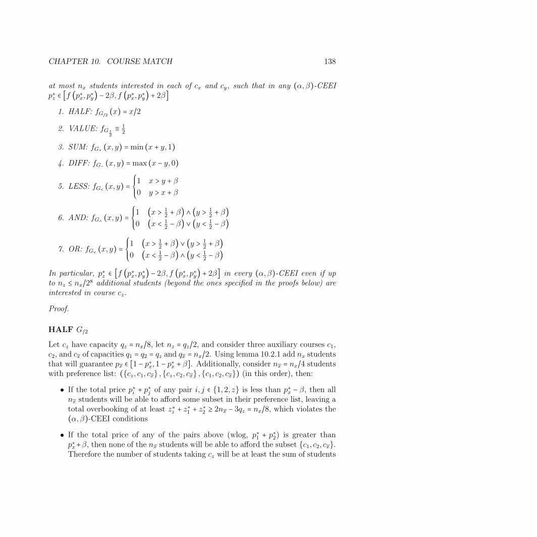
CHAPTER 10. COURSE MATCH 138
at most nx students interested in each of cx and cy, such that in any (α,β)-CEEIp∗z ∈ [f (p∗x, p∗y) − 2β, f (p∗x, p∗y) + 2β]
1. HALF: fG/2 (x) = x/2
2. VALUE: fG 12
≡ 12
3. SUM: fG+ (x, y) = min (x + y,1)
4. DIFF: fG− (x, y) = max (x − y,0)
5. LESS: fG< (x, y) =⎧⎪⎪⎨⎪⎪⎩
1 x > y + β0 y > x + β
6. AND: fG∧ (x, y) =⎧⎪⎪⎨⎪⎪⎩
1 (x > 12 + β) ∧ (y > 1
2 + β)0 (x < 1
2 − β) ∨ (y < 12 − β)
7. OR: fG∨ (x, y) =⎧⎪⎪⎨⎪⎪⎩
1 (x > 12 + β) ∨ (y > 1
2 + β)0 (x < 1
2 − β) ∧ (y < 12 − β)
In particular, p∗z ∈ [f (p∗x, p∗y) − 2β, f (p∗x, p∗y) + 2β] in every (α,β)-CEEI even if upto nz ≤ nx/28 additional students (beyond the ones specified in the proofs below) areinterested in course cz.
Proof.
HALF G/2
Let cz have capacity qz = nx/8, let nz = qz/2, and consider three auxiliary courses c1,c2, and cx of capacities q1 = q2 = qz and qx = nx/2. Using lemma 10.2.1 add nx studentsthat will guarantee px ∈ [1 − p∗x,1 − p∗x + β]. Additionally, consider nx = nx/4 studentswith preference list: (cz, c1, cx ,cz, c2, cx ,c1, c2, cx) (in this order), then:
• If the total price p∗i + p∗j of any pair i, j ∈ 1,2, z is less than p∗x − β, then allnx students will be able to afford some subset in their preference list, leaving atotal overbooking of at least z∗z + z∗1 + z∗2 ≥ 2nx − 3qz = nx/8, which violates the(α,β)-CEEI conditions
• If the total price of any of the pairs above (wlog, p∗1 + p∗2) is greater thanp∗x+β, then none of the nx students will be able to afford the subset c1, c2, cx.Therefore the number of students taking cz will be at least the sum of students

CHAPTER 10. COURSE MATCH 139
taking c1 or c2. Therefore, even after taking into account nz additional students,we have that z∗z + z∗1 + z∗2 ≥ qz − nz = nx/16.
VALUE G 12
Similarly to the HALF gadget, consider two auxiliary courses c1 and c2, and let nxstudents have preferences: (cz, c1 ,cz, c2 ,c1, c2). Then, following the argumentfor the HALF gadget, it is easy to see that p∗z ∈ [1
2 ,12 + β] in any (α,β)-CEEI, with
nz = nx/8.
DIFF G−
Let cx be a course with price p∗x ∈ [1 − p∗x,1 − p∗x + β], qx = nx/2, and consider nx = nx/4students willing to take cx, cy, cz. Then it is easy to see that
p∗z ∈ [1 − p∗x − p∗y ,1 − p∗x − p∗y + β]⊆ [p∗x − p∗y − β, p∗x − p∗y + β]
with nz = nx/16
SUM G+
Concatenating NOT and DIFF gadgets, we have:
p∗x ∈ [1 − p∗x,1 − p∗x + β]p∗z ∈ [p∗x − p∗y − β, p∗x − p∗y + β]p∗z ∈ [1 − (p∗x − p∗y + β) ,1 − (p∗x − p∗y − β) + β]
⊆ [p∗x + p∗y − 2β, p∗x + p∗y + 2β]for nz = nx/28
LESS G<
Let cx be a course with price p∗x ∈ [1 − p∗x,1 − p∗x + β], qx = nx/2; let qz = nx/8 andnz = nx/16. Consider nx/4 students wishing to take (cx, cycz), in this order:
• If p∗y > p∗x + β, then p∗x + p∗y > 1+ β, and therefore none of the nx/4 students willbe able to afford the first pair; they will all try to sign up to cz which will beoverbooked unless p∗z > 1
• If p∗x > p∗y +β, then all nx/4 students will sign up for the first pair, forcing p∗z = 0in any (α,β)-CEEI.

CHAPTER 10. COURSE MATCH 140
AND G∧
Let c 12
be a course with price p∗12
∈ [12 ,
12 + β] and n 1
2= nx/8, as guaranteed by gadget
VALUE; let qz = nx/32 and nz = nx/64. Consider nx/16 students wishing to take
(cx, c 12 ,cy, c 1
2 ,cz), in this order.
• If (p∗x > 12 + β) ∧ (p∗y > 1
2 + β), then the nx/16 students can afford neither pair.They will all try to sign up for cz, forcing p∗z > 1, in any (α,β)-CEEI.
• If (x < 12 − β) ∨ (y < 1
2 − β), then the nx/16 students can afford at least one ofthe pairs and will register for those courses. Thus p∗z = 0.
OR G∨
Similar to the AND gadget; students will want (cx, cy, c 12 ,cz), in this order.
10.3 A-CEEI ∈ PPADthat the problem belongs to the class PPAD; this proof is much harder than usual.
In this section we establish that computing a (√σM2 , β)-CEEI is in PPAD, for
σ = min2k,M. We follow the steps of the existence proof in [Bud11], and showthat each one can be carried out either in polynomial time, or through a fixed point.One difficulty is that certain steps of Budish’s proof are randomized and must beconstructively derandomized in polynomial time.
Remark 10.3.1. We assume that the student preferences (≿i) are given in the form ofan ordered list of all the bundles in Ψi (i.e., all the bundles that student i prefers overthe empty bundle). In particular, we assume that the total number of permissiblebundles is polynomial.
Remark 10.3.2. In fact, we prove that the following, slightly more general problem,is in PPAD: Given any β, ε > 0 and initial approximate-budgets vector b ∈ [1,1 + β]N ,
find a (√σM2 , β)-CEEI with budgets b∗ such that ∣bi − b∗i ∣ < ε for every i.
Our proof will follow the steps of the existence proof by [Bud11]. We will use thepower of PPAD to solve the Kakutani problem, and derandomize the other noncon-structive ingredients.

CHAPTER 10. COURSE MATCH 141
10.3.1 Preliminaries
Our algorithm receives as input an economy ((qj)Mj=1 , (Ψi)Ni=1 , (≿i)Ni=1), parameters
β, ε > 0, and an initial approximate-budgets vector b ∈ [1,1 + β]N . We denote β =minβ, ε/2.
We will consider M -dimensional price vectors in P = [0,1 + β + ε]M . In order todefine a price adjustment function, we consider an enlargement P = [−, + β + ε]M, aswell as a truncation function t ∶ P → P (whose j-th coordinate is given by tj(pj) =minmaxpj,0,1 + β + ε).
For each student i, we denote her demand at prices p with budget bi by
di (p, bi) = max(≿i) x′ ∈ Ψi∶ p ⋅ x′ ≤ bi
Given the total demand of all the students, we can define the excess demand to be:
z (p,b) =N
∑i=1
di (p, bi) − q
A key ingredient to the analysis is the budget-constraint hyperplanes. Theseare the hyperplanes in price space along which a student can exactly afford a spe-cific bundle. For each student i and bundle x, the corresponding budget-constrainthyperplane is defined as H (i, x) = p ∈ P ∶ p ⋅ = .
10.3.2 Deterministically finding a “general position”perturbation (step 1)
It is convenient to assume that the budget-constraint hyperplanes are in “generalposition”, i.e. there is no point p ∈ P at which any subset of linearly dependentbudget-constraint hyperplanes intersect (in particular, no more than M hyperplanesintersect at any point). In the existence proof, this is achieved by assigning a smallrandom reverse tax τi,x ∈ (−ε, ε), for each student i and bundle x; i’s modified costfor bundle x at prices p becomes p ⋅x− τi,x. Given taxes τ = (τi,x)i∈S,x∈Ψi , we redefinedi (p, bi, τi), z (p,b, τ), and H (i, x, τi,x) analogously.
In this section, we show how to deterministically choose these taxes.
Lemma 10.3.3. There exists a polynomial-time algorithm that finds a vector of taxesτ = (τi,x)i∈S,x∈Ψi such that:
1. −ε < τi,x < ε (taxes are small)
2. τi,x > τi,x′ if x ≻i x′ (taxes prefer more-preferred bundles)

CHAPTER 10. COURSE MATCH 142
3. 1 ≤ mini,x bi + τi,x ≤ maxi,x bi + τi,x ≤ 1 + β (inequality bound is preserved)
4. bi + τi,x ≠ bi′ + τi′,x′ for (i, x) ≠ (i′, x′) (no two perturbed prices are equal)
5. there is no price p ∈ P at which any subset of linearly dependent budget-constraint hyperplanes intersect1
Proof. Assume wlog that b is rounded to the nearest integer multiple of βM−M :otherwise we can include this rounding in the taxes.
We proceed by induction on the pairs (i, x) of students and bundles: at eachstep let τi,x be much smaller in absolute value than all the taxes introduced so far.(For each i, we consider the (i, x)’s either in the order ≿i or in the reverse order,maintaining Property 2 depending on the sign of τi,x.)
More precisely, if (i, x) is the νth pair to be considered, then we set
τi,x ∈ ±βM−2νM ,
where the sign is chosen such that condition 3 in the statement of the lemma ispreserved.
Now, assume by contradiction that there exists a k-tupleH (i1, x1, τi1,x1) , . . . ,H (ik, xk, τik,xk)of hyperplanes that intersect at price vector p, and such that the xi’s are linearlydependent. (Note that the latter holds, in particular, for every (M + 1)-tuple.)
Assume further, wlog, that this is the first such k-tuple, with respect to theorder of the induction. In particular, this means that x1, . . . , xk−1
are linearlyindependent. Now consider the system
( xT1 . . . xTk−1 ) (α) = (xk)
Notice that it has rank k − 1. We can now take k − 1 linearly independent rowsj1, . . . jk−1 such that the following system has the same unique solution α:
⎛⎜⎝
x1,j1 . . . xk−1,j1
⋮ ⋱x1,jk−1
xk−1,jk−1
⎞⎟⎠(α) =
⎛⎜⎝
xk,j1⋮
xk,jk−1
⎞⎟⎠
Denote
X =⎛⎜⎝
x1,j1 . . . xk−1,j1
⋮ ⋱x1,jk−1
xk−1,jk−1
⎞⎟⎠
1 The original existence proof of [Bud11] requires only that no more than M hyperplanesintersect at any point; this causes problems in the conditional expectation argument [Bud11, Step5].

CHAPTER 10. COURSE MATCH 143
Since X is a square matrix of full rank it is invertible, so we have that
α =X−1⎛⎜⎝
xk,j1⋮
xk,jk−1
⎞⎟⎠
Now, recall that
X−1 = 1
detX
⎛⎜⎝
X1,1 . . . Xk−1,1
⋮ ⋱X1,k−1 Xk−1,k−1
⎞⎟⎠
where Xi,j is the (i, j)-cofactor of X. Finally, since X is a Boolean matrix, its deter-
minant and all of its cofactors are integers of magnitude less than (k − 1)k−1 ≤MM .The entries of α are therefore rational fractions with numerators and denominatorsof magnitude less than MM .
Now, by our assumption by contradiction, k hyperplanes intersect at p:
⎛⎜⎝
x1
⋮xk
⎞⎟⎠(p) =
⎛⎜⎝
bi1 + τi1,x1
⋮bik + τik,xk
⎞⎟⎠
Therefore,
bik + τik,xk = xk ⋅ p =k−1
∑l=1
αl (xl ⋅ p) =k−1
∑l=1
αl (bil + τil,xl) (10.1)
However, if (ik, xk) is the νth pair added by the induction, then the following is aninteger:
k−1
∑l=1
(det(X) ⋅ αl) ⋅M2(ν−1)M
β(bil + τil,xl)
By our assumption that all the budgets are rounded, MM
β⋅ bik is also an integer. Yet
∣det(X) ⋅ M2(ν−1)M
β⋅ τik,xk ∣ ≤ ∣M(2ν−1)M
β⋅ τik,xk ∣ ≤ M−M is not an integer. This yields a
contradiction to Equation (10.1).
10.3.3 Finding a fixed point (steps 2-4)
This subsection describes the price adjustment correspondence of [Bud11], and isbrought here mostly for completeness.
We first define the price adjustment function:
f (p) = t (p) + 1
2Nz (t (p) ;b, τ)

CHAPTER 10. COURSE MATCH 144
Observe that if p∗ is a fixed point p∗ = f (p∗) of f , then its truncation t (p∗) = p∗
defines an exact competitive equilibrium2. Yet, we know that the economy may nothave an exact equilibrium - and indeed f is discontinuous at the budget constrainthyperplanes, and so it is not guaranteed to have a fixed point.
Instead, we define an upper hemicontinuous, set-valued “convexification” of f :
F (p) = coy∶ ∃ a sequence pw → p, p ≠ pw ∈ P such that f (pw)→ y
The correspondence F is upper hemicontinuous, non-empty, and convex; therefore,by Kakutani’s fixed point theorem it has a fixed point (i.e. a price vector that satisfiesp∗ ∈ F (p∗)).
By [Pap94], finding a Kakutani fixed point of F is in PPAD.
Working with finite precision
To be rigorous, we need to complete a few subtle numerical details about findinga fixed point of F . We round all price vectors to a the nearest integer multiple of
δ ∶= (βM 12−2(νmax+1)M) (this precision suffices to implement the algorithm in Lemma
10.3.3).At any point on the δ-grid, the price of any bundle is an integer multiple of δ,
so, any budget-constraint hyperplane which does not contain p, must be at (L1)distance at least δ. In particular, this means that every δ/2-approximate fixed pointof F is also an exact fixed point. Finally, we can use the PPAD algorithm of [Pap94]to find a δ/2-approximate fixed point.
There is also an issue of computing the correspondence F . From the proof of[Pap94] it follows that it suffices to compute just a single point in F (p) for everyp. This is important because the number of points in F (p) on the δ-grid may beexponential. As we mentioned earlier, every budget-constraint hyperplane which doesnot contain t (p), must be at least δ-far. Therefore, we can take any point p′ whosetruncation t (p′) is at distance δ/2 from t (p), and does not lie on any hyperplanes.(p′ will not be on the δ-grid.) Because no budget-constraint hyperplanes lie betweent (p′) and t (p), it follows that t (p) + 1
2N z (t (p′) ;b, τ) ∈ F (p).
10.3.4 From a fixed point to an approximate CEEI (steps5-9)
Lemma 10.3.4. Given a fixed point p∗ of F , we can find in polynomial time a vector
of prices pφ′
such that ∥z (pφ′ ,b, τ)∥2≤
√σM2
2See [Bud11, Appendix A, Step 2] for more details.

CHAPTER 10. COURSE MATCH 145
Proof. We use the method of conditional expectation to derandomize Step 8 of[Bud11].
Recall from the previous subsection that there exists a neighborhood aroundp∗ which does not intersect any budget-constraint hyperplanes (beyond those thatcontain p∗). Let 1, . . . , L′ be the indices of students whose budget-constraint hyper-planes intersect at p∗. For student i ∈ [L′], let wi be the number of corresponding
hyperplanes H (i, x1i , τi,x1
i) , . . .H (i, xwii , τi,xwii ) intersecting at p∗, and assume wlog
that the superindices of x1i , . . . x
wii are ordered according to ≿i.
Let d0i be agent i’s demand when prices are slightly perturbed from p∗ such that
all xji ’s are affordable. Such a perturbation exists and is easily computable becausethe hyperplanes are linearly independent3. Similarly, let d1
i denote agent i’s demandwhen x2
i , . . . xwii are affordable, but x1
i is not, and so on. Finally, let zS∖[L′] (p∗,b, τ) =dS∖[L′] (p∗,b, τ) − q be the market clearing error when considering the rest of thestudents. (The demands of S ∖ [L′] is constant in the small neighborhood p∗ whichdoes not intersect any additional hyperplanes.)
By Lemma 3 of [Bud11], there exist distributions afi over dfi :
afi ∈ [0,1] ∀ i ∈ [L′] ,∀f ∈ 0 ∪ [wi]wi
∑f=0
afi = 1 ∀ i ∈ [L′]
such that the clearing error of the expected demand is 0:
zS∖[L′] (p∗,b, τ) +L′
∑i=1
wi
∑f=0
afi dfi = 0
We first find such afi in polynomial time using linear programming.The existence proof then considers, for each i, a random vector Θi = (Θ1
i , . . . ,Θwii ):
the vectors are independent and in any realization θi satisfy ∑wif=0 θ
fi = 1, while the
variables each have support supp (Θfi ) = 0,1, and expectation E [Θf
i ] = afi .
By Lemma 4 of [Bud11], the expected clearing error is bounded by:
EΘ!...ΘL′
XXXXXXXXXXX
L′
∑i=1
wi
∑f=0
(afi − θfi )d
fi
XXXXXXXXXXX
2
2
=L′
∑i=1
EΘi
XXXXXXXXXXX
wi
∑f=0
(afi − θfi )d
fi
XXXXXXXXXXX
2
2
≤ σM4
3This perturbation eventually guarantees the existence of pφ′. As we mentioned in Footnote
1, Budish does not require that the hyperplanes are linearly independent, so pφ′
may not exist.However, it seems that pφ
′is not actually crucial to the overall existence proof. In particular, as
Budish points out, even if it exists it may be infeasible (i.e. require negative prices), so the finalsolution uses p∗ instead.

CHAPTER 10. COURSE MATCH 146
We now proceed by induction on the students. For each i, if the conditional expec-tation on (θj)j<i satisfies
EΘi...ΘL′
⎡⎢⎢⎢⎢⎣
XXXXXXXXXXX
L′
∑i=1
wi
∑f=0
(afi − θfi )d
fi
XXXXXXXXXXX
2
2
∣ θ1, . . . , θi−1
⎤⎥⎥⎥⎥⎦≤ σM
4
then at least one θi must also satisfy the above bound. We can find such θi inpolynomial time by computing the conditional expectation for every feasible θ
′
i:
EΘi+1...ΘL′
⎡⎢⎢⎢⎢⎣
XXXXXXXXXXX
L′
∑j=1
wj
∑f=0
(afj − θfj )d
fj
XXXXXXXXXXX
2
2
∣ θ1, . . . , θi
⎤⎥⎥⎥⎥⎦=
i
∑j=1
XXXXXXXXXXX
wj
∑f=0
(afj − θfj )d
fj
XXXXXXXXXXX
2
2
+L′
∑j=i+1
EΘj
XXXXXXXXXXX
wj
∑f=0
(afj − θfj )d
fj
XXXXXXXXXXX
2
2
+ ∑j≠h≤i
wj
∑f=0
wh
∑g=0
(afj − θfj ) (a
gh − θ
gh)
Finally, the choice of (θi)L′
i=1induces the promised price vector pφ
′.
The chosen (θi)L′
i=1define an allocation x∗ with bounded clearing error. We now
follow step 9 of [Bud11] in order to define budgets b∗ such that x∗ is the preferredconsumption by all the students at price p∗.
We define, for every i, b∗i = bi + τi,x∗i . For i > L′ we have x∗i = di (p∗, bi, τi). Byrequirement 2 of lemma 10.3.3, every bundle that student i prefers over x∗i had agreater tax and was still unaffordable at p∗; it now costs more than bi + τi,x∗i .
For i ≤ L′ notice that every bundle x⊥i that i prefers over x∗i and was exactlyaffordable at p∗ with taxes τ and budget b, x⊥ must cost strictly more than i’s new
budget b∗i . Therefore, (x∗,b∗,p∗) is a (√σM2 , β)-CEEI

147
Part IV
Quasi-polynomial Time

148
Chapter 11
Birthday repetition
This part of the thesis deals with several fundamental problems that admit quasi-polynomial (nlogn) time algorithms. What can we learn from such an algorithm? Onone hand, assuming the Exponential Time Hypothesis (ETH, see Hypothesis 1), itmeans that they are not NP-hard. On the other hand, it does not meet our goldstandard of efficiency, polynomial time (P). Furthermore, the logarithmic factor inthe exponent is still prohibitive in applications in practice.
The approach we take in this this thesis is inspired by the birthday repetition meta-reduction due to Aaronson, Impagliazzo, and Moshkovitz [AIM14]. The birthdayrepetition is best explained as a game1 between two provers (Alice and Bob) and averifier. The omniscient but untrusted provers want to convince the verifier that acertain 3-SAT formula is (approximately) satisfiable. The provers agree in advanceon an assignment, and are then placed in separate rooms. The verifier asks Alicefor the assignments of 3 variables on one randomly chosen clause, and asks Bob forthe assignment of one of the variables in the same clause. It is not hard to see thatif at most 90% of the clauses are satisfiable, the provers have probability at most90% to succeed in sending assignments that both satisfy Alice’s clause and agreeon the Bob’s variable. Otherwise, the verifier can detect that Alice and Bob arelying and the 3-SAT formula is not satisfiable. But this requires coordinating thechallenge-messages sent to Alice and Bob.
In the birthday-repetition version of the same two-prover one-verifier game, theverifier sends Alice a random selection of
√n clauses, and sends Bob an indepen-
dently random subset of√n variables. By the birthday paradox, we expect that one
of Bob’s variables appears in one of Alice’s clauses. Thus their probability of trickingthe verifier into believing that a far-from-satisfiable formula is satisfiable is not much
1The sense in which we use the word “game” here is unrelated to the game theoretic “game”.
CHAPTER 11. BIRTHDAY REPETITION 149
higher than in the original (no-repetition) two-prover one-verifier game. The mainadvantage in this approach is that the challenges sent to Alice and Bob are indepen-dent; this is sometimes called a free game. This is particularly helpful when reducingto bilinear optimization problems such as Densest k-Subgraph or Nash equilibrium(recall (1.1) in the introduction).
The other interesting feature of the birthday repetition game is that it blowsup the number of possible questions to Alice and Bob, and (more importantly) thelength of their answers. In particular, given a list of
√n variables, Bob has N ≜ 2
√n
distinct choices of truth assignments to those variables. Therefore, if Alice and Bobcan devise an (approximately) optimal strategy much faster than N logN = 2n, theywould violate ETH. Hence with this approach we can obtain quasi-polynomial lowerbounds on the running time that almost exactly match the running time of the bestknown algorithms.
There is one more property that is common to all our quasi-polynomial lowerbounds: while they are all based on the birthday repetition approach, each problemintroduces new obstacle and requires new ideas.
11.1 Warm-up: best ε-Nash
In order to introduce the “birthday repetition” framework, we begin with a partic-ularly simple application. As we have already discussed, proving hardness of totalproblem is notoriously difficult both conceptually and technically. Often, however,there are related decision problems that admit much easier proofs of intractability.For example, Gilboa and Zemel [GZ89] proved that deciding whether there exists aNash equilibrium with certain welfare guarantees is NP-hard.
By looking at the analogous question for approximate Nash equilibrium, we cir-cumvent the difficulty of totality. But the quasi-polynomial algorithm of [LMM03]can approximately2 solve this question as well. Hence, assuming ETH, this problemis still not NP-hard.
Braverman et al. [BKW15] showed a nearly matching quasi-polynomial lowerbound on the running time for approximating the best ε-Nash equilibrium. Thetheorem below obtains slightly better parameters. More importantly, our proof issignificantly simpler3 .
2This is a bi-criteria approximation: in quasi-polynomial time the algorithm can distinguishbetween a game that has a high-payoff exact (or ε/2)-approximate Nash equilibrium, and a gamewhere every ε-approximate Nash equilibrium has low payoff. Notice however that this does not implythat the algorithm can approximate (to within an additive ε) the value of the best ε-approximateNash equilibrium.
3Briefly, in our proof we focus on a single partition of the variables, where it is guaranteed that
CHAPTER 11. BIRTHDAY REPETITION 150
Theorem 11.1.1. There exists a constant ε > 0 such that, given a two-player, N-strategy game with utilities in [0,1] distinguishing between the following requiresN Ω(logN) time (assuming the Exponential Time Hypothesis):
Completeness The game has an exact Nash equilibrium with expected payoff > 0.99for both players.
Soundness In every ε-approximate Nash equilibrium, both players have expectedpayoff < 0.01.
The rest of this section is devoted to the proof of Theorem 11.1.1. We firstprove a small (O (ε)) additive gap between completeness and soundness. This is themain step that exhibits the birthday repetition. We then achieve a large gap bya simple amplification step, where we introduce a new action for each player, anda spurious low-payoff pure equilibrium: in the completeness case, the players don’twant to deviate from the high-payoff mixed equilibrium; but for the soundness, theyare lured by unilateral deviations into the low-payoff equilibrium.
11.1.1 Constructing the first gap
Lemma 11.1.2. There exist absolute constants ε, δ > 0 such that the following holds.Given a two-player, N-strategy game with utilities in [0,1] distinguishing betweenthe following requires N Ω(logN) time (assuming the Exponential Time Hypothesis):
Completeness The game has an exact Nash equilibrium with expected payoff c forboth players.
Soundness In every ε-Nash equilibrium, at least one player has expected payoff s ≤c − δ.
Proof. We reduce from a bipartite, constant alphabet 2CSP. By the PCP Theo-rem 2.4.1, distinguishing between a completely satisfiable instance and one whereonly (1 − η)-fraction (for some constant η > 0) of the clauses are satisfiable requirestime 2Ω(n), assuming ETH. We construct a game where, at every approximate Nashequilibrium, Alice’s and Bob’s respective mixed strategies encode an assignment (ordistribution over assignments) to the 2CSP4. Alice’s and Bob’s expected payoff willdepend on the number of satisfied clauses.
every pair of subsets induces approximately the right number of constraints. In contrast, [BKW15]enumerate over all the subsets of size ≈
√
n. Then it is only true that most pairs of subsets inducethe right number of constraints, which somewhat complicates the proof.
4Note that so far every approximate equilibrium encodes some assignment (or distribution overassingmnets) - even in the soundness case.

CHAPTER 11. BIRTHDAY REPETITION 151
Construction
At a high level, our construction is composed of three subgames. The main subgamewill test the 2CSP assignment; in this subgame we perform the “birthday repetition”.The remaining two auxiliary subgames enforce the structure of (approximate) equi-libria; in particular, they force that the players to assign (approximately) uniformprobabilities in the main subgame to (almost) all 2CSP variables; this step uses aconstruction due to Althofer [Alt94].
The players’ final payoff is a weighted average of the payoffs in the three subgame.Since we want to make sure that the structural constraints on the equilibria areenforced, we place only ε weight on the main subgame, and weight 1−ε
2 on each of theauxiliary subgames.
Main subgame We partition Alice’s and Bob’s respective sets of variables into√n subsets Si and Tj, respecitively. By Lemma 2.7.6, we can guarantee that
each subset has at most 2√n variables, and that the number of constraints between
any pair Si, Tj is at most 8 times the expectation.In the main subgame, each player, chooses an index i, j ∈ [√n], and a partial
assignment for the corresponding respective subsets σ ∈ ΣASi , τ ∈ ΣB
Tj . If the partialassignments jointly satisfy all the induced constraints, both players receive payoff 1;otherwise they receive payoff 0.
Auxiliary subgames In addition to the choices of i, σ in the main subgame,Alice chooses a subset CA ⊂ [√n] of cardinality ∣CA∣ =
√n/2. In the first auxiliary
subgame, Alice wants to use the set CA to “catch” Bob’s index j: Alice has payoff 1if j ∈ CA, and 0 otherwise. Bob, on the other hand, tries to “escape”: his payoff is 0if j ∈ CA, and 1 otherwise.
The second auxiliary subgame is defined analogously (Bob chooses a set CB ofcardinality ∣CB ∣ =
√n/2 and tries to catch Alice’s index i.)
Analysis
Game size Each player has an action set of size N ≤ √n ⋅ Σ2
√n ⋅ (
√n√n/2) = 2O(√n).
Therefore, assuming ETH, finding an (approximately) satisfying assignment to theLabel Cover instance requires time 2Ω(n) = N Ω(logN).
Completeness If the 2CSP has a satisfying assignment, the players can play thefollowing high-welfare equilibrium: in the main subgame, Alice and Bob choose

CHAPTER 11. BIRTHDAY REPETITION 152
i, j uniformly at random, and σ, τ as the respective restrictions of the satisfyingassignments. In the auxiliary subgames, Alice and Bob choose CA,CB uniformly atrandom.
Because i, j are chosen uniformly at random, they have no incentives to deviatefrom their choice of CA,CB; similarly, since CA,CB are chosen uniformly at random(and the payoff in the main subgame is always 1), neither player has an incentive todeviate from the choice of i, j. Therefore this is indeed a Nash equilibrium.
Finally, the expected payoff for each player in each auxiliary subgame is 1/2(they have probability 1/2 of winning), and 1 in the main subgame; in total it isc ≜ 1/2 + ε/2.
Soundness
First, we claim that in every ε-approximate Nash equilibrium (ε-ANE), the players’respective distributions over i, j are O (ε)-close to uniform. Assume by contradictionthat Alice’s distribution over i is 36ε-far from uniform. By Lemma 2.7.8, Bob can
pick a set CB ∈ ([√n]√n/2) such that i ∈ CB with probability 1/2 + 9ε. Therefore Bob can
guarantee a payoff of at least 1/2 + 9ε from the second auxiliary subgame (withoutaffecting his payoffs from the other subgames). Therefore at any ε-ANE, he guaran-tees himself more than 1/2 + 6ε (otherwise, having a 3ε-improving deviation on theauxiliary subgame implies a > ε-deviation in total). Therefore Alice’s payoff on thissubgame is less than 1/2 − 6ε, whereas she can guarantee herself a payoff of 1/2 bypicking i uniformly at random. Thus she can improve her total payoff by more than2ε, which is a violating deviation even after we subtract ε for potential loss of payoffdue to changing her strategy in the main subgame.
Any mixed strategy profile induces a distribution over assignments to the original2CSP instance: for each set Si, we take the distribution over ΣA
Si induced by Alice’smixed strategy restricted to actions where she picks index i (if she never picks i,choose an arbitrary assignment for Si). Alice’s expected payoff in the main subgameis equal to the probability that an assignment drawn from the induced distributionsatisfies the constraints on a random pair (Si, Tj), where i and j are drawn accordingto Alice and Bob’s respective mixed strategies. Since those strategies are O (ε)-close to uniform, Alice’s expected payoff in the main subgame is within O (ε) of theprobability that the constraints between a uniformly random (Si, Tj) are satisfied.If the value of the 2CSP is 1−η, then the probability that any consistent assignment(in particular, one drawn from the induced distribution) satisfies a uniformly random(Si, Tj) is at most 1 − η/8; this is true because, by our construction of the partition,the η-fraction of unsatisfied constraints cannot concentrate on less than η/8-fractionof pairs. Therefore Alice’s (respectively Bob’s) expected payoff in the main subgame

CHAPTER 11. BIRTHDAY REPETITION 153
is at most 1−η/8+O (ε). Since the auxiliary subgames are 1-sum games, at least oneof Alice or Bob must have total expected payoff at most 1/2 + ε/2 (1 − η/8 +O (ε)) <c − ηε/16 + O (ε2). Choosing ε sufficiently small compared to η (yet still constant)completes the proof.
11.1.2 Gap amplification
Proof of Theorem 11.1.1. Consider the game from Lemma 11.1.2. First, we scale allthe payoffs by a 10−4-factor and shift them so that they are between 1 − 10−4 and 1.Now, by Lemma 11.1.2, it is hard to distinguish between the game having an exactNash equilibrium with expected payoff c′ and every ε′-Nash equilibrium having atleast one player with expected payoff < c′ − δ′. We choose ε sufficiently small; inparticular, ε < ε′/4, δ′/4 < 10−4.
We add one new action to each player. When both players play old actions, theirpayoffs are as in the game from Lemma 11.1.2 (with modified payoffs). When Aliceplays the new action and Bob plays an old action, Alice’s payoff is c′−δ′/2, and Bob’spayoff is 0. Similarly, when Alice plays an old action and Bob plays his new action,Alice’s payoff is 0 and Bob’s payoff is c′ − δ′/2. Finally, when they both play theirnew actions their payoff is 10−3.
Notice that playing the new action is an (exact) pure Nash equilibrium. Noticefurther that when the 2CSP is satisfied, the original equilibrium from the complete-ness of Lemma 11.1.2 is still a Nash equilibrium since the average payoff to bothplayers from that equilibrium is higher than what they would get by deviating to thenew strategy.
To complete the proof we need to argue for soundness. In particular, we claim thatif the value of the 2CSP is only 1 − η, then every ε-approximate Nash equilibrium is10−3-close (in total variation distance) to the new strategy pure equilibrium. Assumeby contradiction that this is not the case, i.e. there is an ε-approximate equilibriumwhere (wlog) Alice assigns probability more than 10−3 to old strategies. First, noticethat Bob must assign at least 1/2 probability to old strategies: whenever Bob playsthe new strategy, Alice has a large incentive to deviate to her new strategy. Therefore,by a symmetric argument, Alice must also assign at least 1/2 probability to oldactions.
Finally, the mixed strategy profile restricted to the old strategies must be a4ε-approximate Nash equilibrium of the scaled old game. By Lemma 11.1.2, theexpected payoff to one of the players is at most c′ − δ′. But then that player has atleast δ′/4 > ε incentive to deviate to her new strategy.

154
Chapter 12
Densest k-Subgraph
k-Clique is one of the most fundamental problems in computer science: given agraph, decide whether it has a fully connected induced subgraph on k vertices. Sinceit was proven NP-complete by Karp [Kar72], extensive research has investigated thecomplexity of relaxed versions of this problem.
This work focuses on two natural relaxations of k-Clique which have receivedsignificant attention from both algorithmic and complexity communities: The firstone is to relax “k”, i.e. looking for a smaller subgraph:
Problem 12.0.1 (Approximate Max Clique, Informal). Given an n-vertex graph G,decide whether G contains a clique of size k, or all induced cliques of G are of sizeat most δk for some 1 > δ(n) > 0.
The second natural relaxation is to relax the “Clique” requirement, replacing it withthe more modest goal of finding a subgraph that is almost a clique:
Problem 12.0.2 (Densest k-Subgraph with perfect completeness, Informal). Givenan n-vertex graph G containing a clique of size k, find an induced subgraphs of G ofsize k with (edge) density at least (1 − ε), for some 1 > ε > 0. (More modestly, givenan n-vertex graph G, decide whether G contains a clique of size k, or all inducedk-subgraphs of G have density at most (1 − ε)).
Today, after a long line of research [Fei+96; AS98; Aro+98; Has99; Kho01; Zuc07]we have a solid understanding of the inapproximability of Problem 12.0.1. In partic-ular, we know that it is NP-hard to distinguish between a graph that has a clique ofsize k, and a graph whose largest induced clique is of size at most k′ = δk for δ = 1/n1−ε
[Zuc07]. The computational complexity of the second relaxation (Problem 12.0.2)remained largely open. There are a couple of (very different) quasi-polynomial algo-rithms that guarantee finding a (1 − ε)-dense k subgraph in every graph containing

CHAPTER 12. DENSEST k-SUBGRAPH 155
a k-clique [FS97; Bar15], suggesting that this problem is not NP-hard. Yet we knowneither polynomial-time algorithms, nor general impossibility results for this prob-lem.
In this work we provide a strong evidence that the aforementioned quasi-polynomialtime algorithms for Problem 12.0.2 [FS97; Bar15] are essentially tight, assuming the(deterministic) Exponential Time Hypothesis (ETH) (Hypothesis 1). In fact, we showthat under ETH, both parameters of the above relaxations are simultaneously hardto approximate:
Theorem 12.0.3 (Main Result). There exists a universal constant ε > 0 such that,assuming the (deterministic) Exponential Time Hypothesis, distinguishing betweenthe following requires time nΩ(logn), where n is the number of vertices of G.
Completeness G has an induced k-clique; and
Soundness Every induced subgraph of G size k′ = k ⋅ 2−Ω( lognlog logn
) has density at most1 − ε,
Our result has implications for two major open problems whose computationalcomplexity remained elusive for more than two decades: The (general) Densestk-Subgraph problem, and the Planted Clique problem.
Densest k-Subgraph
The Densest k-Subgraph problem, DkS (η, ε), is the same as (the decision ver-sion of) Problem 12.0.2, except that in the “completeness” case, G has a k-subgraphwith density η, and in the “soundness” case, every k-subgraph is of density at mostε, where η ≫ ε. Since Problem 12.0.2 is a special case of this problem, our maintheorem can also be viewed as a new inapproximability result for DkS (1,1 − ε). Weremark that the aforementioned quasi-polynomial algorithms for the “perfect com-pleteness” regime completely break in the sparse regime, and indeed it is believed thatDkS (n−α, n−β) (for k = nε) in fact requires much more than quasi-polynomial time[Bha+12]. The best to-date approximation algorithm for Densest k-Subgraphdue to Bhaskara et. al, is guaranteed to find a k-subgraph whose density is withinan ∼ n1/4-multiplicative factor of the densest subgraph of size k [Bha+10], and thusDkS (η, ε) can be solved efficiently whenever η ≫ n1/4 ⋅ε (this improved upon a previ-ous n1/3−δ-approximation of Feige et. al [FKP01]). Making further progress on eitherthe lower or upper bound frontier of the problem is a major open problem.
Several inapproximability results for Densest k-Subgraph were known againstspecific classes of algorithms [Bha+12] or under incomparable assumptions of Unique

CHAPTER 12. DENSEST k-SUBGRAPH 156
Games with expansion [RS10] and hardness of random k-CNF [Fei02; Alo+11]. Themost closely related result is by Khot [Kho06], who shows that the Densest k-Subgraph problem has no PTAS unless SAT can be solved in time 2n
ε, as opposed
to 2n1/2+ε
in our paper. While Khot’s work uses a slightly weaker assumption, animportant advantage of our work is simplicity: our construction is very simple, es-pecially in contrast to Khot’s reduction.
We stress that the result of [Kho06], as well as other aforementioned works,focus on the sub-constant density regime, i.e. they show hardness for distinguishingbetween a graph where every k-subgraph is sparse, and one where every k-subgraphis even sparser. In contrast, our result has perfect completeness and provides thefirst additive inapproximability for Densest k-Subgraph — the best one can hopefor as per the upper bound of [Bar15].
Planted Clique
The Planted Clique problem is a special case of our problem, where the inputscome from a specific distribution (G (n, p) versus G (n, p)+ “a planted clique of sizek”, where p is some constant1). The Planted Clique Conjecture ([Alo+07; AKS98;Jer92; Kuc95; FK00; DGGP10]) asserts that distinguishing between the aforemen-tioned cases for p = 1/2, k = o(√n) cannot be done in polynomial time, and has servedas the underlying hardness assumption in a variety of recent applications includingmachine-learning and cryptography (e.g. [Alo+07; BR13]) that inherently use theaverage-case nature of the problem, as well as in reductions to worst-case problems(e.g. [HK11; Alo+11; KZ11; Bal+13; Che+15a; Bad+16]).
The main drawback of average-case hardness assumptions is that many average-case instances (even those of worst-case-hard problems) are in fact tractable. Inrecent years, the centrality of the planted clique conjecture inspired several worksthat obtain lower bounds in restricted models of computation [Fel+13; MPW15;DM15; Hop+16; Bar+16]. Nevertheless, a general lower bound for the average-caseplanted clique problem appears out of reach for existing techniques. Therefore, animportant potential application of our result is replacing average-case assumptionssuch as the planted-clique conjecture, in applications that do not inherently rely onthe distributional nature of the inputs (e.g., when the ultimate goal is to prove aworst-case hardness result). In such applications, there is a good chance that plantedclique hardness assumptions can be replaced with a more “conventional” hardnessassumption, such as the ETH, even when the problem has a quasi-polynomial algo-
1 Planted Clique typically refers to p = 1/2, while our hardness result is analogous to p = 1−δ,for a small constant δ > 0. Nevertheless, in almost all applications of Planted Clique, hardnessfor any constant p suffices.

CHAPTER 12. DENSEST k-SUBGRAPH 157
rithm. Recently, such a replacement of the planted clique conjecture with ETH wasobtained for the problem of finding an approximate Nash equilibrium with approxi-mately optimal social welfare [BKW15].
We also remark that, while showing hardness for Planted Clique from worst-case assumptions seems beyond the reach of current techniques, our result can also beseen as circumstantial evidence that this problem may indeed be hard. In particular,any polynomial time algorithm (if exists) would have to inherently use the (rich andwell-understood) structure of G (n, p).
Followup work by Manurangsi
The soundness in our result was greatly improved by Manurangsi [Man17], whoshowed that even DkS (1, n−1/poly log logn) may be intractable; i.e. in the NO case themaximal density is almost inverse-polynomial.
Techniques
Our simple construction is inspired by the “birthday repetition” technique: givena 2CSP (e.g. 3COL), we have a vertex for each Ω (√n)-tuple of variables andassignments (respectively, 3COL vertices and colorings). We connect two vertices byan edge whenever their assignments are consistent and satisfy all 2CSP constraintsinduced on these tuples. In the completeness case, a clique consists of choosingall the vertices that correspond to a fixed satisfying assignment. In the soundnesscase (where the value of the 2CSP is low), the “birthday paradox” guarantees thatmost pairs of vertices (i.e. two Ω (√n)-tuples of variables) will have a significantintersection (nonempty CSP constraints), thus resulting in lower densities wheneverthe 2CSP does not have a satisfying assignment. In the language of two-provergames, the intuition here is that the verifier has a “constant chance in catching theplayers in a lie if they are trying to cheat” in the game while not satisfying the CSP.
While our construction is simple, analyzing it is intricate. The main challengeis to rule out a “cheating” dense subgraph that consists of different assignments tothe same variables (inconsistent colorings of the same vertices in 3COL). Intuitively,this is similar in spirit to proving a parallel repetition theorem where the provers cananswer some questions multiple times, and completely ignore other questions. Con-tinuing with the parallel repetition metaphor, notice that the challenge is doubled:in addition to a cheating prover correlating her answers (the standard obstacle toparallel repetition), each prover can now also correlate which questions she choosesto answer. Our argument follows by showing that a sufficiently large subgraph mustaccumulate many non-edges (violations of either 2CSP or consistency constraints).
CHAPTER 12. DENSEST k-SUBGRAPH 158
To this end we introduce an information theoretic argument that carefully countsthe entropy of choosing a random vertex in the dense subgraph.
We note that our entropy-based argument is completely different from all otherknown applications of “birthday repetition” to other problems. The main reasonis that enforcing consistency is much more difficult in the case of Densest k-Subgraph than in other applications because the problem formulation is so simple.In fact, even the follow-up work on the same problem by [Man17] used a completelydifferent (and quite elegant) argument that is based on counting small bi-cliques inany given subgraph.
12.1 Construction (and completeness)
12.1.1 Construction
Let ψ be the 2CSP instance produced by the reduction in Theorem 2.4.4, i.e. aconstraint graph over n variables with alphabet A of constant size. We construct thefollowing graph Gψ = (V,E):
• Let ρ ∶= √n log logn and k ∶= (n
ρ).
• Vertices of Gψ correspond to all possible assignments (colorings) to all ρ-tuples of variables in ψ, i.e V = [n]ρ × Aρ. Each vertex is of the form v =(yx1 , yx2 , . . . , yxρ) where x1, . . . , xρ are the chosen variables of v, and yxi isthe corresponding assignment to variable xi.
• If v ∈ V violates any 2CSP constraints, i.e. if there is a constraint on (xi, xj)in ψ which is not satisfied by (yxi , yxj), then v is an isolated vertex in Gψ.
• Let u = (yx1 , yx2 , . . . , yxρ) and v = (y′x′1 , y′x′2, . . . , y′x′ρ). (u, v) ∈ E iff:
– (u, v) does not violate any consistency constraints: for every shared vari-able xi, the corresponding assignments agree, yxi = y′xi ;
– and (u, v) also does not violate any 2CSP constraints: for every 2CSP
constraint on (xi, x′j) (if exists), the assignment (yxi , y′x′j) satisfy the con-
straint.
Notice that the size of our reduction (number of vertices of Gψ) is N = (nρ) ⋅ ∣A∣ρ =
2O(√n).

CHAPTER 12. DENSEST k-SUBGRAPH 159
Completeness If OPT(ψ) = 1, then Gψ has a k-clique: Fix a satisfying assignmentfor ψ, and let S be the set of all vertices that are consistent with this assignment.Notice that ∣S∣ = (n
ρ) = k. Furthermore its vertices do not violate any consistency
constraints (since they agree with a single assignment), or 2CSP constraints (sincewe started from a satisfying assignment).
12.2 Soundness
Suppose that OPT(ψ) < 1−η, and let ε0 > 0 be some constant to be determined later.We shall show that for any subset S of size k′ ≥ k ⋅ ∣V ∣−ε0/ log log ∣V ∣, den(S) < 1 − δ,where δ is some constant depending on η. The remainder of this section is devotedto proving the following theorem:
Theorem 12.2.1. If OPT(ψ) < 1 − η, then ∀S ⊂ V of size k′ ≥ k ⋅ ∣V ∣−ε0/ log log ∣V ∣,den(S) < 1 − δ for some constant δ.
12.2.1 Setting up the entropy argument
Fix some subset S of size k′, and let v ∈R S be a uniformly chosen vertex in S (recallthat v is a vector of ρ coordinates, corresponding to labels for a subset of ρ chosenvariables). For i ∈ [n], let Xi denote the indicator variable associated with v suchthat Xi = 1 if the i’th variable appears in v and 0 otherwise. We let Yi representthe coloring assignment (label) for the i’th variable whenever Xi = 1, which is of theform l ∈ A. Throughout the proof, let
Wi−1 =X<i, Y<i
denote the i’th prefix corresponding to v. We can write :
H(Yi∣Wi−1,Xi) = Pr[Xi = 0] ⋅H(Yi∣Wi−1,Xi = 0)+Pr[Xi = 1] ⋅H(Yi∣Wi−1,Xi = 1)
= Pr[Xi = 1] ⋅H(Yi∣Wi−1,Xi = 1)
since H(Yi∣Wi−1,Xi = 0) = 0. Notice that since (XY ) and v determine each other,and v was uniform on a set of size ∣S∣ = k′, we have
Observation 12.2.2. H(XY ) = log k′.
Thus, in total, the choice of challenge and the choice of assignments should con-tribute log k′ to the entropy of v. If much of the entropy comes from the assignment

CHAPTER 12. DENSEST k-SUBGRAPH 160
distribution (conditioned on the fixed challenge variables), we will show that S musthave many consistency violations, implying that S is sparse. If, on the other hand,almost all the entropy comes from the challenge distribution, we will show thatthis implies many CSP constraint violations (implied by the soundness assumption).From now on, we denote
αi ∶=H(Xi∣X<i, Y<i) and βi ∶=H(Yi∣X≤i, Y<i).
When conditioning on the i’th prefix, we shall write αi(wi−1) ∶=H(Xi∣X<i, Y<i = wi−1),and similarly for βi(⋅). Also for brevity, we denote
qi ∶= Pr[Xi = 1] and qi(wi−1) ∶= Pr[Xi = 1∣wi−1].
Prefix graphs
The consistency constraints induce, for each i, a graph over the prefixes: the verticesare the prefixes, and two prefixes are connected by an edge if their labels are consis-tent. (We can ignore the 2CSP constraints for now — the prefix graph will be usedonly in the analysis of the consistency constraints.) Formally,
Definition 12.2.3 (Prefix graph). For i ∈ [n+1] let the i-th prefix graph, Gi = (Vi,Ei)be defined over the prefixes of length i− 1 as follows. We say that wi−1 is a neighborof σi−1 if they do not violate any consistency constraints. Namely, for all j < i, ifXj = 1 for both wi−1 and σi−1, then wi and σi assign the same label Yj.
In particular, we will heavily use the following notation: let N (wi−1) be the prefixneighborhood of wi−1; i.e. it is the set of all prefixes (of length i−1) that are consistentwith wi−1. For technical issues of normalization, we let wi−1 ∈ N (wi−1), i.e. all theprefixes have self-loops.
Notice that Gn+1 is defined over the vertices of S (the original subgraph). Theset of edges on S is contained in the set of edges of Gn+1, since in the latter we onlyremove pairs that violated consistency constraints (recall that we ignore the 2CSPconstraints).
Unless stated otherwise, we always think of prefixes as weighted by their proba-bilities. Naturally, we also define the weighted degree and weighted edge density ofthe prefix graph.
Definition 12.2.4 (Prefix degree and density). The prefix degree of wi−1 is given by:
deg(wi−1) = ∑σi−1∈N (wi−1)
Pr[σi−1].
CHAPTER 12. DENSEST k-SUBGRAPH 161
Similarly, we define the prefix density of Gi as:
den(Gi) = ∑wi−1
∑σi−1∈N (wi−1)
Pr[wi−1] ⋅Pr[σi−1].
When it is clear from the context, we henceforth drop the prefix qualification,and simply refer to the neighborhood or degree, etc., of wi−1.
Notice that in Gn+1, the probabilities are uniformly distributed. In particular,den(Gn+1) ≥ den(S), since, as we mentioned earlier, the set of edges in S is containedin that of Gn+1. Finally, observe also that because we accumulate violations, thedensity of the prefix graphs is monotonically non-increasing with i.
Observation 12.2.5.
den(G1) ≥ ⋅ ⋅ ⋅ ≥ den(Gn+1) ≥ den(S).
Useful approximations
We use the following bounds on αi and βi many times throughout the proof:
Fact 12.2.6.αi = E [H(qi(wi−1))] ≤H(E [qi(wi−1)]) =H(qi)
Fact 12.2.7.βi = E [βi(wi−1))] ≤ E [qi(wi−1) ⋅ log ∣A∣] = qi log ∣A∣
Proof. The bound on αi follows from concavity of entropy (Fact 2.6.3). For thesecond bound, observe that βi is maximized by spreading qi mass uniformly overalphabet A.
We also recall some elementary approximations to logarithms and entropies thatwill be useful in the analysis. The proofs are deferred to the appendix.
Fact 12.2.8. For k = (nρ) then,
log k = nH (ρn) ±O (logn) = (1
2− o (1))ρ logn
More useful to us will be the following bounds on log k′:
Fact 12.2.9. Let ε1 ≥ 5ε0, and k, k′, V, n, ρ as specified in the construction. Then,
log k′ ≥ maxlog k,nH (ρn) − ε1 log k/ logn
´¹¹¹¹¹¹¹¹¹¹¹¹¹¹¹¹¹¹¹¹¹¹¹¹¹¹¹¹¹¹¸¹¹¹¹¹¹¹¹¹¹¹¹¹¹¹¹¹¹¹¹¹¹¹¹¹¹¹¹¹¹¶≈ ε1
2⋅ρ
.
This means that most indices i should contribute roughly H ( ρn) entropy to the choice
of v.

CHAPTER 12. DENSEST k-SUBGRAPH 162
We will also need the following bound which relates the entropies of a very biasedcoin and a slightly less biased one:
Fact 12.2.10. Let 1/n≪ ∣υ∣ ≪ 1. Then
H (1 + υn
) =H ( 1
n) − υ
nlog
1
n− (log e) υ
2
2n
+O (n−2) +O (υ3
n)
A useful lemma: bias implies less entropy
In Fact 12.2.6 we saw that always αi ≤ H(qi). Equality happens only if the qi-mass is evenly distributed across all prefixes. We argue that if qi is far from evenlydistributed, then the inequality is also far from tight. In particular:
Claim 12.2.11. Let B ⊂ Vi be a subset of prefixes such that for some 0 < a < b < 1,
1. ∑wi−1∈B Pr[wi−1] ≤ b; but also
2. ∑wi−1∈B Pr[wi−1]qi (wi−1) > a.
Then αi ≤H(qi) − qiDKL (a∥b).
Proof. Abusing notation, let B(⋅) be the indicator variable for Wi−1 ∈ B. By thedata-processing inequality (Fact 2.6.8),
αi = H (Xi ∣Wi−1)≤ H (Xi ∣ B(Wi−1))= H (Xi) − I (Xi;B(Wi−1)) (12.1)
Since we can write mutual information as expected KL-divergence (Fact 2.6.10), andKL-divergence is non-negative, we get
I(Xi;B(Wi−1)) = Exi [DKL (B(Wi−1)∣xi∥B(Wi−1))]
≥ qiDKL (Pr[B(Wi−1) = 1 ∣xi = 1]∥B(Wi−1) = 1)
≥ qiDKL (a∥b),
where the second inequality follows from the premise assumptions that Pr[B(Wi−1)] ≤b and Pr[B(Wi−1 = 0 ∣ xi = 1] ≥ a

CHAPTER 12. DENSEST k-SUBGRAPH 163
Plugging into (12.1) we have:
αi ≤H (qi) − qiDKL (a∥b). (12.2)
12.2.2 Consistency violations
In this section, we show that if the total entropy contribution of the assignments(∑i βi)) is large, there are many consistency violations between vertices, which leadto constant density loss. First, we show that if ∑i βi > 5ε1 log k/ logn, then at leasta constant fraction of such entropy is concentrated on good variables that contributeto both “types” of entropy.
Definition 12.2.12 (Good Variables). We say that an index i is good if
• αi ≥H(qi) − 2qi log ∣A∣
• βi ≥ 12ε1qi
where ε1 is a constant to be determined later in the proof.
Claim 12.2.13. For any constant ε1, if ∑i βi > 5ε1 log k/ logn,
∑good i’s
q2i ≥ (1
5ε1ρ)
2
/(n log2 ∣A∣) = Ω(ρ2/n).
Proof. We want to show that many of the indices i have both a large αi and a largeβi simultaneously. Let ι ⊆ [n] denote the set of i such that αi +βi <H (qi)− qi log ∣A∣.We can write
∑i∈[n]
(αi + βi) =∑i∈ι
(αi + βi) +∑i∉ι
(αi + βi)
Using Facts 12.2.6 and 12.2.7, we have
∑i∈[n]
(αi + βi) ≤∑i∈ι
(H (qi) − βi) +∑i∉ι
(H (qi) + βi) .
Because the subgraph is of size k′, from the expansion of log k′ (Fact 12.2.9),
∑i∈[n]
(αi + βi) ≥ nH (ρn) − ε1 log k/ logn
≥∑H (qi) − ε1 log k/ logn,

CHAPTER 12. DENSEST k-SUBGRAPH 164
where the second inequality follows from the concavity of entropy. Plugging into(12.2.2), we have
∑i∉ιβi ≥∑
i∈ιβi − ε1 log k/ logn
= (∑i
βi −∑i∉ιβi) − ε1 log k/ logn
Rearranging, we get
∑i∉ιβi ≥
1
2∑i
βi − ε1 log k/ logn (12.3)
For all the i’s in the LHS summation, αi ≥H (qi)−2qi log ∣A∣ by Fact 12.2.7. Fromnow on, we will consider only i’s that satisfy this condition. Now, using the premiseon ∑i βi and (12.3) we have:
∑i∶αi≥H(qi)−2qi log ∣A∣
βi ≥ (5/2 − 1)ε1 log k/ logn
≥ 0.7ε1ρ,
where the second inequality follows from our approximation for log k (Fact 12.2.8).We want to further restrict our attention to i’s for which βi is at least 1
2ε1qi (akagood i’s). Note that the above inequality can be decomposed to
∑good i’s
βi + ∑i∶αi≥H(qi)−2qi log ∣A∣
βi< 12ε1qi
βi ≥ 0.7ε1ρ
Now via a simple sum bound,
∑i∶αi≥H(qi)−2qi log ∣A∣
βi< 12ε1qi
βi ≤1
2ε1∑
i
qi =1
2ε1ρ
Rearranging, we get,
∑good i’s
βi ≥1
5ε1ρ
By Cauchy-Schwartz we have:
∑good i’s
β2i ≥ (1
5ε1ρ)
2
/n

CHAPTER 12. DENSEST k-SUBGRAPH 165
Finally, since βi ≤ qi log ∣A∣,
∑good i’s
q2i ≥ (1
5ε1ρ)
2
/(n log2 ∣A∣).
In the same spirit, we now define a notion of a “good” prefix. Intuitively, con-ditioning on a good prefix leaves a significant amount of entropy on the i’th index.We also require that a good prefix has a high prefix degree; that is, it has manyneighbors it could potentially lose when revealing the i-th label.
Definition 12.2.14 (Good Prefixes). We say wi−1 is a good prefix if:
• i is good;
• ∑σi−1∈N (wi−1) qi(σi−1)Pr[σi−1] ≥ (1 − ε2)qi;
• βi(wi−1) ≥ ε3qi(wi−1),
for ε3 = (ε4+κ) log ∣A∣, with ε4 an arbitrarily small constant that denotes the fractionof assignments that disagree with the majority of the assignments, κ = Θ(1/ log ∣A∣),and ε2 a constant that satisfies δ = ( ε2
∣A∣2/ε2 )4, with den(S) = 1 − δ.
In the following claim, we show that these prefixes contribute some constantfraction of entropy, assuming that our subset is dense.
Claim 12.2.15. If den(S) > 1 − δ, where δ = ( ε2∣A∣2/ε2 )
4and ε1 ≥ 4ε2 log ∣A∣ + 8ε3, then
for every good index i, it holds that
∑good wi−1’s
Pr[wi−1]βi (wi−1) ≥ βi/4
Proof. We begin by proving that most prefixes satisfy the degree condition of Def-inition 12.2.14. Let wi−1 be popular if i is a good variable and its degree in theprefix graph Gi is at least deg(wi−1) ∶= ∑σi−1∈N (wi−1) Pr[σi−1] ≥ 1 −
√δ. Recall that
den(Gi) ≥ den(S) ≥ (1 − δ) (by Observation 12.2.5). Thus by Markov inequality, atmost
√δ-fraction of the prefixes are unpopular.
We now argue that:
∑unpopular wi−1’s
Pr[wi−1]qi (wi−1) ≤ ε2qi. (12.4)

CHAPTER 12. DENSEST k-SUBGRAPH 166
Otherwise, by Claim 12.2.11, αi ≥ H (qi) − qiDKL (ε2∥√δ). On the other hand,
recall that since i is good, αi ≥H (qi) − 2qi log ∣A∣. Recall also that δ = ( ε2∣A∣2/ε2 )
4, and
therefore DKL (ε2∥√δ) ≥ 2 log ∣A∣. Thus, we get a contradiction.
Ineq. (12.4) implies that even if the assignment is uniform over the alphabet, thecontribution to ∑βi from unpopular prefixes is small:
∑unp.
Pr[wi−1]βi (wi−1) ≤ ∑unp.
Pr[wi−1]qi (wi−1) log ∣A∣
≤ ε2qi log ∣A∣
≤ 1
4ε1qi ≤ 1
2βi
where first inequality follows from Fact 12.2.7, second from (12.4), third from oursetting of ε1 ≥ 4ε2 log ∣A∣, and fourth from βi ≥ 1
2ε1qi since i is good. Therefore,
∑pop.
Pr[wi−1]βi (wi−1) = βi − ∑unp.
Pr[wi−1]βi (wi−1)
≥ βi/2
Using a similar argument, we show that for any popular wi−1, most of the qimass is concentrated on its neighbors. Consider any popular wi−1, and let NC (wi−1)denote the complement of N (wi−1). Then we can rewrite αi as:
αi = ∑σi−1∈N (wi−1)
Pr[σi−1]αi (σi−1)
+ ∑σi−1∈NC(wi−1)
Pr[σi−1]αi (σi−1)
Notice that since wi−1 is popular, NC (wi−1) has measure at most√δ. Thus, if an
ε2-fraction of the qi mass is concentrated on NC (wi−1), Claim 12.2.11 implies:
αi ≤H (qi) − qiDKL (ε2∥√δ),
which (as in (12.4)) would yield a contradiction to i being a good variable. Thereforeevery popular prefix also satisfies the qi-weighted condition on the degree:
∑σi−1∈N (wi−1)
Pr[σi−1]qi (σi−1) ≥ (1 − ε2) qi (12.5)

CHAPTER 12. DENSEST k-SUBGRAPH 167
Recall that a prefix wi−1 is good if it also satisfies βi (wi−1) ≥ ε3 ⋅ qi (wi−1). For-tunately, prefixes that violate this condition (i.e. those with small βi (wi−1)), cannotaccount for much of the weight on βi:
∑βi(wi−1)<ε3qi(wi−1)
Pr[wi−1]βi (wi−1) ≤ ε3qi.
Since i is good and ε1 ≥ 8ε3, this implies:
∑good wi−1’s
Pr[wi−1]βi (wi−1) ≥ βi/2 − ε3qi ≥ βi/4
since
ε3qi ≤1
8ε1qi ≤
1
4βi
where last inequality follows from i being good.
Corollary 12.2.16. For every good index i,
∑good wi−1’s
Pr[wi−1]qi (wi−1) ≥ε1
8 log ∣A∣qi.
Proof.
∑good
Pr[wi−1]qi (wi−1) ≥ ∑good
Pr[wi−1]βi/ log ∣A∣
≥ βi/(4 log ∣A∣)≥ ε1
8 log ∣A∣qi.
Where the first inequality follows by Fact 12.2.7, the second by Claim 12.2.15, andthe last by definition of good i’s.
With Claim 12.2.13 and Corollary 12.2.16, we are ready to prove the main lemmaof this section:
Lemma 12.2.17 (Labeling Entropy Bound). If ∑iH(Yi∣X≤i, Y<i) > 5ε1 log klogn , then
den(S) < 1 − δ.
Proof. Assume for a contradiction that den(S) ≥ 1 − δ. For prefix wi−1, let Dwi−1
denote the induced distribution on labels to the i-th variable, conditioned on wi−1
and xi = 1. (If qi(wi−1) = 0, take an arbitrary distribution.) After revealing eachvariable i, the loss in prefix density is given by the probability of “fresh violations”:

CHAPTER 12. DENSEST k-SUBGRAPH 168
the sum over all prefix edges (wi−1, σi−1) of the probability that they assign differentlabels to the i-th variable:
den(Gi) − den(Gi+1) = ∑wi−1
∑σi−1∈N (wi−1)
. . . (12.6)
(Pr[wi−1]Pr[σi−1]qi(wi−1)qi(σi−1)) PrYi∼Dwi−1Y ′i ∼Dσi−1
[Yi ≠ Y ′i ]
We now lower-bound PrDwi−1×Dσi−1[Yi ≠ Y ′
i ] for good wi−1 (notice that we assumenothing about σi−1). A simple calculation shows that for κ < 1/2, if
βi(wi−1) ≥(κ log ∣A∣ − κ logκ − (1 − κ) log(1 − κ)) qi(wi−1),
then the probability mass (under D(wi−1)) on the most common label is at most1−κ. Observe that this probability is an upper bound on PrDwi−1×Dσi−1
[Yi = Y ′i ]. For
good wi−1, we indeed have
βi(wi−1) ≥ ε3qi(wi−1) ≥(ε4 log ∣A∣ − ε4 log ε4 − (1 − ε4) log(1 − ε4)) qi(wi−1),
where the second inequality follows from choice of ε4. Therefore PrDwi−1×Dσi−1[Yi ≠
Y ′i ] ≥ ε4.
We now have, for every good index i,
den(Gi) − den(Gi+1) ≥ ∑good wi−1’s
∑σi−1∈N (wi−1)
ε4⋅
⋅ (Pr[wi−1]Pr[σi−1]qi(wi−1)qi(σi−1))
≥ ε4qi(1 − ε2) ∑good wi−1’s
Pr[wi−1]qi(wi−1)
≥ ε1ε4
10 log ∣A∣q2i ,
where the first inequality follows by Eq. (12.6); the second definition of good prefix;and the last by Corollary 12.2.16 and ε2 < 0.2.

CHAPTER 12. DENSEST k-SUBGRAPH 169
Finally, summing over all good i’s, we get a negative density for S, which is, ofcourse, a contradiction. By Observation 12.2.5 we have:
1 − den(S) ≥ den(G1) − den(Gn+1)=∑
i
den(Gi) − den(Gi+1)
≥ ∑good i’s
den(Gi) − den(Gi+1)
≥ ∑good i’s
( ε1ε4
10 log ∣A∣) q2i
≥ ( ε31ε4
250 log3 ∣A∣)ρ2/n = Ω(ρ2/n),
where the last inequality follows by Claim 12.2.13.
12.2.3 2CSP violation
Intuitively, if ∑iH(Xi∣X<i, Y<i) is large, then the subgraph approximately corre-sponds to assignments to all subsets in ([n]
ρ). More specifically, in this section we
show that most of the constraints appear approximately as frequently as we expect.Since in any assignment, a constant fraction of them must be violated, this implies(eventually) that a constant fraction of the edges have a violated constraint.
First, we show that most of the variables appear approximately as frequently aswe expect by showing that most of them are “typical.”
Definition 12.2.18 (Typical variables). Prefix wi−1 is typical if
(1 − ε5) ⋅ ρ/n < Pr[Xi = 1∣wi−1] < (1 + ε5) ⋅ ρ/n,
where ε5 is some constant such that ( log e8
) ε45 > 14ε1.
Similarly, we say that variable xi is typical if
∑typical wi−1’s
Pr[wi−1] ≥ 1 − ε5
Claim 12.2.19. If ∑iH(Xi∣X<i, Y<i) ≥ (1 − 6ε1logn) log k = log k − Θ(ρ), then all but at
most ε5n variables are typical.

CHAPTER 12. DENSEST k-SUBGRAPH 170
Proof. Assume by contradiction that there are ε5n atypical variables. That is ε5n/2variables xi appear with probability at least (1 + ε5) ⋅ ρ/n (or at most (1 − ε5) ⋅ ρ/n)for an (ε5/2)-fraction of the prefixes wi−1. Now, subject only to this constraint andmaintaining the correct expected number of variables in each vertex, the entropy ismaximized by spreading the (ε3
5/4)-loss in frequency evenly across all other prefixesand variables. That is on the atypical prefixes, labels are assigned with probability
(1 + ε5)ρ/n, and with probability (1 − ε35/41−ε25/4
)ρ/n on the rest. Thus,
∑i
H(Xi∣X<i, Y<i) <ε2
5
4n ⋅H ((1 + ε5)ρ/n) + (1 − ε
25
4)nH ((1 − ε3
5/41 − ε2
5/4)ρ/n)
Recall from Fact 12.2.10 the expansion of the entropy function:
H (1 + υn
) =H ( 1
n) − υ
nlog
1
n− ( log e
2) υ
2
n+O (n−2) +O (υ
3
n)
Therefore,
∑i
H(Xi∣X<i, Y<i) < ε25
4n [H (ρ
n) − ε5
ρ
nlog
ρ
n− ( log e
2) ρn⋅ ε2
5 +O ((ρn)
2
) +O (ρnε3
5)]
+(1 − ε25
4)n [H (ρ
n) + ( ε3
5/41 − ε2
5/4) ρn
logρ
n+O ((ρ
n)
2
) +O (ρnε6
5)]
= n [H (ρn) − ( log e
8) ρn⋅ ε4
5 +O ((ρn)
2
) +O (ρnε5
5)]
Recall that −2 log ρn < logn. Thus for ( log e
8) ε4
5 > 14ε1, we have that
( log e
8) ρn⋅ε4
5−O ((ρn)
2
)−O (ρnε5
5) >ρ
n⋅12ε1 > −
ρ
nlog
ρ
n⋅24ε1/ logn > (12ε1/ logn)H (ρ
n)
and therefore,
∑i
H(Xi∣X<i, Y<i) < (1 − 12ε1/ logn)nH (ρn) < (1 − 6ε1/ logn) log k,
where the second inequality follows from Fact 12.2.8. Thus we have reached a con-tradiction. Notice that the ( log e
8) ρn ⋅ε4
5 term of missing entropy is symmetric (but notthe negligible higher order terms); i.e. the same derivation can be used to show acontradiction when many variables appear with probability less than (1 − ε5)ρ/n.
Definition 12.2.20. Let I(u, v) be defined as the number of (i, j) pairs such that

CHAPTER 12. DENSEST k-SUBGRAPH 171
• In the original 2CSP instance ψ, there exists an edge (constraint) betweentypical variables xi and xj.
• Xi = 1 for u and Xj = 1 for v.
• ui−1 and vj−1 are typical prefixes, where ui−1 denotes the prefix represented byu for X<i, Y<i, similarly for vj−1.
Intuitively, I(u, v) is the number of “tests” of 2CSP-constraints between verticesu, v, when restricting to typical prefixes and variables. We now use the properties oftypical prefixes and constraints to show that I(u, v) behaves “nicely”.
Claim 12.2.21. Eu,v [I (u, v)] ≥ (1 − ε7)ρ2/n and Eu,v [I2 (u, v)] ≤ (1 + 2ε7)d4 (Eu,v [I (u, v)])2,
where ε7 is some constant ε7 ≥ 6ε5 +Θ(ε25).
Proof. For any i, j ∈ [n], we say that i ∈ N 2CSP (j) if there is a constraint on (xi, xj).For the proof of this claim, we also abuse notation and denote i ∈ v when i is typical,vi−1 is a typical prefix, and Xi = 1 for v. We also say that i ∈ N (u) if i is atypical variable, i ∈ N 2CSP (j), and j ∈ u (for some j ∈ [n]). (Do not confuse thisnotation with prefix neighborhood in the prefix graph.) We can now lower boundthe expectation of I (u, v) as:
Eu,v [I (u, v)] ≥ Eu
⎡⎢⎢⎢⎢⎣∑
i∈N (u)Prv
[i ∈ v]⎤⎥⎥⎥⎥⎦
Notice that this bound may not be tight since any i ∈ v can potentially have dneighbors in u. Thus our upper bound is:
Eu,v [I (u, v)] ≤ d ⋅ Eu⎡⎢⎢⎢⎢⎣∑
i∈N (u)Prv
[i ∈ v]⎤⎥⎥⎥⎥⎦
By definition of typical variables, for each typical i, i ∈ v with probability at least(1 − ε5)2
ρ/n; thus,
Eu,v [I (u, v)] ≥ Eu
⎡⎢⎢⎢⎢⎣∑
i∈N (u)(1 − ε5)2
ρ/n⎤⎥⎥⎥⎥⎦= (1 − ε5)2
ρ/n ⋅ Eu [∣N (u)∣] (12.7)
All but ε5n variables are typical, so all but 2ε5n variables are typical and have atleast one typical neighbor. We restrict our attention to the set of such variables and

CHAPTER 12. DENSEST k-SUBGRAPH 172
fix one typical neighbor for each; this neighbor appears in u with probability at least(1 − ε5)2
ρ/n. Therefore,
Eu [∣N (u)∣] ≥ (1 − 2ε5)n ⋅ ((1 − ε5)2ρ/n) ≥ (1 − 4ε5)ρ (12.8)
Combining (12.7) and (12.8), we get the desired bound:
Eu,v [I (u, v)] ≥ ((1 − ε5)2ρ/n) (1 − 4ε5)ρ ≥ (1 − ε7)ρ2/n. (12.9)
Similarly, for the variance we have
Eu,v [I2 (u, v)] ≤ d2 ⋅ Eu,v⎛⎝ ∑i∈v∩N (u)
1⎞⎠
2
= d2 ⋅ Eu,v⎡⎢⎢⎢⎢⎣
∑i≠j∈v∩N (u)
1 + ∑i∈v∩N (u)
1
⎤⎥⎥⎥⎥⎦
≤ d2 ⋅ Eu⎡⎢⎢⎢⎢⎣2 ∑i<j∈N (u)
Prv
[i ∈ v]Prv
[j ∈ v ∣ i ∈ v]⎤⎥⎥⎥⎥⎦+ d2 ⋅ Eu,v [I (u, v)] .
Since for every prefix, each variable receives a typical assignment with probability atmost (1 + ε5) ⋅ ρ/n, we have that
Eu,v [I2 (u, v)] ≤ 2d2 ⋅ Eu⎡⎢⎢⎢⎢⎣∑
i<j∈N (u)((1 + ε5) ⋅ ρ/n)2
⎤⎥⎥⎥⎥⎦+ d2 ⋅ Eu,v [I (u, v)]
≤ ((1 + ε5) ⋅ ρ/n)2 ⋅ 2d2 ⋅ Eu(∣N (u) ∣
2) + d2 ⋅ Eu,v [I (u, v)](12.10)
We would like to bound Eu(N (u)2
).
Eu(N (u)
2) = ∑
i<j∑
k∈N 2CSP (i)∑
l∈N 2CSP (j)Pru
[k ∈ u]Pru
[l ∈ u ∣ k ∈ u]
= ∑i<j
∑k∈N 2CSP (i)l∈N 2CSP (j)and k<l
Pru
[k ∈ u]Pru
[l ∈ u ∣ k ∈ u] (12.11)
+∑i<j
∑k∈N 2CSP (i)l∈N 2CSP (j)and k>l
Pru
[l ∈ u]Pru
[k ∈ u ∣ l ∈ u] (12.12)
+∑i<j
∑k∈N 2CSP (i)∩N 2CSP (j)
Pru
[k ∈ u] (12.13)

CHAPTER 12. DENSEST k-SUBGRAPH 173
For the first two summands, we can use the condition on the prefixes to concludethat
(12.11) + (12.12) ≤ (n2)d2 ((1 + ε5) ⋅ ρ/n)2
Whereas to bound the third summand we first change the order of summation:
(12.13) = ∑k
Pru
[k ∈ u] ⋅ ∣(i, j) ∶ i ≠ j and k ∈ N 2CSP (i) ∩N 2CSP (j)∣
≤ ((1 + ε5) ⋅ ρ) (d
2) = O (ρ)
Summing the last two inequalities, we have
2 ⋅ Eu(∣N (u)∣
2) ≤ d2 ((1 + ε5) ⋅ ρ)2 +O (ρ) ≤ (1 + ε5)3
d2ρ2
Plugging back into (12.10):
Eu,v [I2 (u, v)] ≤ (1 + ε5)5d4ρ4/n2 + d2 ⋅ Eu,v [I (u, v)]
Using (12.9) and the fact that ρ = √n log logn≫ √
n, this gives
Eu,v [I2 (u, v)] ≤ d4(1 + ε5)5
1 − ε7
(Eu,v [I (u, v)])2 + d2 ⋅ Eu,v [I (u, v)]
≤ (1 + 2ε7)d4 (Eu,v [I (u, v)])2
It will also be convenient to count the number of tests between a pair of variables.
Definition 12.2.22. For any pair of typical (i, j) ∈ ψ, let I⊺(i, j) be defined as thenumber of (u, v) ∈ (S × S) pairs such that
• Xi = 1 for u and Xj = 1 for v.
• ui−1 and vj−1 are typical prefixes, where ui−1 denotes the prefix represented byu for X<i, Y<i, similarly for vj−1.
We now have two ways to count the total number of tests between typical prefixesto typical variables:
Observation 12.2.23. ∑(u,v)∈(S×S) I(u, v) = ∑(i,j)∈ψ I⊺(i, j).Furthermore, since i and j are typical, the number of tests between also behaves
“nicely”:

CHAPTER 12. DENSEST k-SUBGRAPH 174
Observation 12.2.24. For every typical (i, j) ∈ ψ, we have I⊺(i, j) ∈ ∣S∣2ρ2/n2[ (1 − ε5)4, (1 + ε5)2 ].
Proof.
I⊺(i, j) = ∑typical ui−1’s
∣S∣ ⋅Pr[ui−1]Pr [Xi = 1 ∣ ui−1] ∑typical vj−1’s
∣S∣ ⋅Pr [vj−1]Pr [Xj = 1 ∣ vj−1]
∈ ∣S∣2ρ2/n2[ (1 − ε5)4, (1 + ε5)2 ].
Armed with these Claims 12.2.19 and 12.2.21 and Observations 12.2.23 and12.2.24, we are now ready to prove the main lemma of this section. Recall thatthe soundness of the 2CSP we started with is 1 − η for a small constant η.
Lemma 12.2.25. If ∑iH(Xi∣X<i, Y<i) ≥ (1 − 6ε1logn) log k, then δ(S) < 1 − δ, where
δ < ε26d4(1+2ε7) and ε6 = (η/2 − ε5) (1/∣A∣2) (1−ε5)4
(1+ε5)2 .
Proof. Let the mode assignment be the assignment A∶ [n] → A which assigns toeach variable xi its most common typical assignment (i.e. assignment after a typicalprefix), breaking ties arbitrarily. In particular, at least 1/∣A∣ of the typical assign-ments for xi are equal to A (i). Of course, this assignment cannot satisfy more thana (1 − η)-fraction of the constraints in the original 2CSP; after removing the ε5natypical variables, (η/2 − ε5)dn constraints out of the dn/2 constraints must still beunsatisfied.
Recall that the number of tests for each constraint over typical variables, I⊺(i, j),is approximately the same for every pair of (i, j) — up to a (1−ε5)4
(1+ε5)2 -multiplicative fac-
tor (Observation 12.2.24). Therefore, the total fraction of tests over unsatisfied con-straints, out of all tests, is approximately proportional to the fraction of unsatisfiedconstraints:

CHAPTER 12. DENSEST k-SUBGRAPH 175
∑typical,unsatisfied(i, j)’s
I⊺(i, j) ≥ (1 − ε5)4
(1 + ε5)2 ⋅∣typical, unsatisfied (i, j)’s∣
∣typical (i, j) ∈ ψ∣⋅ ∑(i,j)∈ψ
I⊺(i, j)
≥ (1 − ε5)4
(1 + ε5)2 ⋅(η/2 − ε5)dn
dn/2 ⋅ ∑(i,j)∈ψ
I⊺(i, j)
= (1 − ε5)4
(1 + ε5)2 ⋅ (η − 2ε5) ⋅ ∑(u,v)∈(S×S)
I(u, v) (Observation 12.2.23)
For each such pair (i, j), on at least a 1/∣A∣2-fraction of the tests both variablesreceive the mode assignment, so the constraint is violated2. Thus the total number
of violations is at least ε6∑(u,v)∈(S×S) I (u, v) (where ε6 = (η/2 − ε5) (1/∣A∣2) (1−ε5)4
(1+ε5)2 ).
Finally, we show that so many violations cannot concentrate on less than a δ-fraction of the pairs u, v ∈ S; otherwise:
∑(u,v)∈(S×S)∖E
I2 (u, v) ≥ 1
δ ∣S∣2⎛⎝ ∑(u,v)∈(S×S)∖E
I (u, v)⎞⎠
2
(Cauchy-Schwartz)
≥ 1
δ ∣S∣2⎛⎝ε6 ∑
(u,v)∈(S×S)I (u, v)
⎞⎠
2
= ∣S∣2ε26
δ(Eu,v [I (u, v)])2
;
yet by Claim 12.2.21,
∑(u,v)∈(S×S)∖E
I2 (u, v) ≤ ∑(u,v)∈S×S
I2 (u, v) ≤ (1 + 2ε7)d4∣S∣2 (Eu,v [I (u, v)])2.
Thus we have a contradiction since d4(1 + 2ε7) < ε26/δ by our setting of δ. Therefore
we have 2CSP-violations in more than a δ-fraction of the pairs u, v ∈ S.
With Lemma 12.2.17 and Lemma 12.2.25, we can now complete the proof ofTheorem 12.2.1.
2We remark that a more careful analysis of the expected number of violations would allow oneto save an ∣A∣
2-factor in the value of ε6. Since it does not qualitatively affect the result, we opt forthe simpler analysis.

CHAPTER 12. DENSEST k-SUBGRAPH 176
Proof of Theorem 12.2.1. Recall that∑iαi+βi = log k′ ≥ (1− ε1logn) log k by Fact 12.2.9.
If ∑i βi > ( 5ε1logn) log k, then by Lemma 12.2.17, δ(S) < 1 − δ. Otherwise, if ∑iαi >
(1 − 6ε1logn) log k, by Lemma 12.2.25, δ(S) < 1 − δ.

177
Chapter 13
Community detection
Identifying communities is a central graph-theoretic problem with important appli-cations to sociology and marketing (when applied to social networks), biology andbioinformatics (when applied to protein interaction networks), and more (see e.g.Fortunato’s classic survey [For10]). Defining what exactly is a community remainsan interesting problem on its own (see Arora et al [Aro+12] and Borgs et al [Bor+16]for excellent treatment from a theoretical perspective). Ultimately, there is no sin-gle “right” definition, and the precise meaning of community should be different forsocial networks and protein interaction networks.
In this paper we focus on the algorithmic questions arising from one of the simplestand most canonical definitions, which has been considered by several theoreticalcomputer scientists [Mis+08; Aro+12; Bal+13] (see Subsection 13.0.1 for furtherdiscussion):
Definition 13.0.1 ((α,β)-Community). Given an undirected graph G = (V,E) an(α,β)-community is a subset S ⊆ V that satisfies:
Strong ties inside the community For every v ∈ S, ∣v × S∣ ∩E ≥ α ⋅ ∣S∣; and
Weak ties to nodes outside the community For every u ∉ S, ∣u × S∣ ∩ E ≤β ⋅ ∣S∣.
Arora et al [Aro+12, Theorem 3.1] gave a simple quasi-polynomial (nO(logn)) timefor detecting (α,β)-communities whenever α − β is at least some positive constant.Similar to the meta-algorithm we described in the introduction, [Aro+12]’s algorithmenumerates over O (logn)-tuples of vertices. For each tuple, consider the set ofvertices that are neighbors of an (α + β) /2-fraction of the tuple; test whether thiscandidate set is indeed a community.
CHAPTER 13. COMMUNITY DETECTION 178
Here we show that, for every constants α > β ∈ (0,1], community detection re-quires quasi-polynomial time (assuming ETH). For example, when α = 1 and β = 0.01,this means that we can hide a clique C, such that every single vertex not in C isconnected to at most 1% of C. Our main result is actually a much stronger inapprox-imability: even in the presence of a (1, o (1))-community, finding any (β + o (1) , β)-community is hard.
Theorem 13.0.2. For every n there exists an ε = ε (n) = o (1) such that, assumingETH, distinguishing between the following requires time nΩ(logn):
Completeness G contains an (1, ε)-community; and
Soundness G does not contain an (β + ε, β)-community for any β ∈ [0,1].
Unlike many related quasi-polynomial approximation schemes mentioned above,Arora et al’s algorithm has the unique property that it can also exactly count all the(α,β)-communities. Our second result is that counting even the number of (1, o (1))-communities requires quasi-polynomial time. A nice feature of this result is that wecan base it on the much weaker #ETH assumption, which asserts that counting thesatisfying assignment for a 3SAT instance requires time 2Ω(n). (Note, for example,that #ETH is likely to be true even if P = NP.)
Theorem 13.0.3. For every n there exists an ε = ε (n) = o (1) such that, assuming#ETH, counting (1, ε)-communities requires time nlog1−o(1) n.
13.0.1 Related works
The most closely related work is a reduction by Balcan, Borgs, Braverman, Chayes,and Teng [Bal+13, Theorem 5.3] from Planted Clique to finding (1,1 − γ)-communities,for some small (unspecified) constant γ > 0. Note that our inapproximability inTheorem 13.0.2 is much stronger in all parameters; furthermore, although formallyincomparable, our ETH assumption is preferable over the average-case hardness as-sumption of Planted Clique.
Algorithms for special cases
Mishra, Schreiber, Stanton, and Tarjan [Mis+08] gave a polynomial-time algorithmfor finding (α,β)-communities that contain a vertex with very few neighbors outsidethe community. Balcan et al [Bal+13] give a polynomial-time algorithm for enu-merating (α,β)-communities in the special case where the degree of every node isΩ (n).

CHAPTER 13. COMMUNITY DETECTION 179
Arora, Ge, Sachdeva, and Schoenebeck [Aro+12] consider several semi-randommodels where the edges inside the community are generated at random, accordingto the expected degree model. (In fact, their quasi-polynomial time algorithm isalso stated in this setting, but only their “Gap Assumption”, which is equivalent toα − β = Ω (1), is used in the analysis.)
Stochastic Block Model
Variants of the community detection problem on graphs generated by different stochas-tic models are extremely popular (see e.g. [BBV16; Ban+16; Che+16; FP16; HWX16;MMV16; MPW16; MX16; Tre+16] for papers in conference proceedings from June2016). Perhaps the most influential is the Stochastic Block Model [HLL83]: Thegraph is partitioned into two disjoint communities; the edges within each communityare present with probability α, independently, whereas edges between communitiesare present with probability β. Hence this model can also be seen as a special caseof the (α,β)-Community Detection problem.
Stochastic models are extremely helpful in physics, for example, because atoms’interactions obey simple mathematical formulas with high precision. Unfortunately,for applications such as social networks, existing models do not describe humanbehavior with atomic precision, hence casting a shadow over the applicability ofalgorithms that work on ideal stochastic models. Recent works [MPW16; MMV16]attempted to bridge the gap from ideal model to practice by showing that certainSDP-based algorithms continue to work in a particular semi-random model wherea restricted adversary is allowed to modify the random input graph. These successstories beg the question of how strong can one make the adversary? The currentpaper illuminates some of the computational barriers.
Alternative approaches to modeling communities
As we mentioned above, there are many different definitions of “communities” innetworks. For in-depth discussion of different definitions see Arora et al [Aro+12]or Borgs et al [Bor+16]. As pointed out by the latter, for some definitions evenverifying that a candidate subset is a community is intractable.
There is also an important literature on axiomatic approaches to the relatedproblem of clustering (e.g. [Kle02; BA08; LM14]); note that while clustering typi-cally aims to partition a set of nodes, our main focus is on detecting just a singlecommunity; in particular, different communities may intersect.

CHAPTER 13. COMMUNITY DETECTION 180
13.0.2 Overview of proofs
A good starting point for the technical discussion is the reduction reduction from3SAT to the related problem of Densest-k-Subgraph we describe in Chapter 12.Let us recall the main two ingredients in that reduction: “birthday repetition”[AIM14] and the “FGLSS graph” [Fei+96].
“Birthday repetition” Starting with an instance of Label Cover (see defini-tion in Section 2.4), the reduction considers a mega-variable for every ρ-tupleof variables, for ρ ≈ √
n. By the birthday paradox, almost every pair of ρ-tuples of variables intersect, inducing a consistency constraint on the two mega-assignments. Similarly, we expect to see some Label Cover edges in the unionof the two ρ-tuples, inducing an additional Label Cover constraint betweenthe two mega assignments. Notice that we have (n
ρ) ≈ 2
√n mega variables, and
the alphabet size is also approximately N = 2√n. Therefore, assuming ETH,
finding an approximately satisfying assignment for the mega-variables requirestime 2Ω(n) ≈ N logN .
FGLSS Similarly to the classic reduction by Feige et al. [Fei+96] for the Cliqueproblem, In Chapter 12, we construct a vertex for each mega assignment toeach mega variable, and draw an edge between two vertices if the induced as-signments do not violate any consistency or Label Cover constraints. Noticethat if the Label Cover instance has a satisfying assignment, then the graphcontains a clique of size (n
ρ) where each mega variable receives the mega as-
signment induced by the globally satisfying assignment. On the other hand,any subgraph that corresponds to a consistent assignment which violates manyconstraints must be missing most of its edges.
Unfortunately, this simple reduction is still quite far from working for the Commu-nity Detection problem. Below we describe some of the obstacles and outlinehow we overcome them.
Completeness
Surprisingly, the main problem with using the same reduction for Community De-tection is the completeness: even if the Label Cover instance has a satisfyingassignment, the resulting graph has no (α,β)-communities, for any constants α > β!Observe, in particular, that the clique that corresponds to the satisfying assignmentdoes not satisfy the weak ties condition. For any vertex v in that clique, considerany vertex v′ that corresponds to changing the assignment to just one variable xi in

CHAPTER 13. COMMUNITY DETECTION 181
v’s assignment. If v agrees with the assignments of all other vertices in the clique,v′ agrees with almost all of them - except for the negligible fraction that cover xi orits neighbors in the Label Cover graph.
To overcome this problem of vertices that are “just outside the community”,we use error correcting codes. Namely, we encode each assignment as a low-degreebivariate polynomial over finite field G of size ∣G∣ ≈ √
n. Now vertices correspond tolow-degree assignments to rows/columns of the polynomial. This guarantees that theassignments induced by every two vertices are far. If v agrees with all other verticesin the community, then almost all of those vertices disagree with v′.
Soundness
The main challenge for soundness is ruling out communities that do not correspondto a single, globally consistent assignment to the Label Cover instance. The keyidea is to introduce auxiliary vertices that punish such communities by violating theweak ties desideratum.
Let us begin with the reduction to the counting variant (Theorem 13.0.3), which iseasier, mostly because we are not concerned with approximation (i.e. we only haveto show that subsets that are exactly (1, ε)-communities correspond to satisfyingassignments). Here we further simplify matters by sketching a construction withweighted edges. The full reduction (Section 13.1) uses unweighted edges and is onlyslightly more involved. Consider, for every g ∈ G, an auxiliary vertex that is ε-connected to all proper vertices that do not correspond to assignments to the g-throw/column. Now if a (1, ε)-community C does not contain a vertex with assignmentto the g-th row/column, the auxiliary vertex must simultaneously: (i) belong to C soas not to violate the weak ties desideratum; yet (ii) it cannot belong to C because allits edges have weight ε (this would violate the strong ties desideratum). Thereforeevery (1, ε)-community assigns values to every row/column in G2.
The reduction we described above suffices to show that (assuming ETH) decidingwhether the graph contains a (1, ε)-community also requires quasi-polynomial time.To get the stronger statement of Theorem 13.0.2 we must rule out even (β, β + ε)-communities in case the Label Cover instance is far from satisfiable. In particular,we need to show that subsets that do not correspond to unique, consistent assign-ments are never (β, β + ε)-communities. Instead of a single column/row, we let eachproper vertex correspond to a subset of t ≈ logn columns/rows. Instead of a singleg ∈ G, each auxiliary vertex corresponds to subset H ⊂ G of size ∣H ∣ = ∣G∣ /2. Wedraw an edge between an auxiliary vertex and a proper vertex if the indices of allt columns/rows are contained in H; if they are picked randomly this only happenswith polynomially small probability. If, however, a β-fraction of the community

CHAPTER 13. COMMUNITY DETECTION 182
is restricted to a small subset R ⊂ G, then there are auxiliary vertices for H ⊇ Rthat connect to all those nodes and violate the weak ties desideratum. Roughly,we show that at least a (1 − β)-fraction of the vertices have assignments that are“well spread” over G2, and among those assignments there are many violations ofthe Label Cover constraints.
13.1 Hardness of counting communities
Theorem 13.1.1. There exists an ε (n) = o (1) such that, assuming #ETH, counting(1, ε)-communities requires time nlog1−o(1) n.
Construction
Begin with an instance (A,B,E,π) of Label Cover of size n = nA + nB wherenA ≜ ∣A∣ and nB ≜ ∣B∣. Let G be a finite field of size
√n/ε3, and let F ⊂ G be an
arbitrary subset of size ∣F ∣ = √n. We identify between A∪B and points in F2; we also
identify between a subset of G and ΣA∪ΣB. Thus there is a one-to-one correspondencebetween a subset of assignments to PF ∶F2 → G and assignments to the Label Coverinstance. We can extend any such PF to an individual-degree-(∣F ∣ − 1) polynomialP ∶ G2 → G. In the other direction, we think of each low individual degrees polynomialP ∶ G2 → G as a (possibly invalid) assignment to the Label Cover instance.
For every g ∈ G, and degree-(∣F ∣ − 1) polynomials p1, p2 ∶ G → G such that p1 (g) =p2 (g), we construct 1/ε vertices vg,p1,p2,i
1/εi=1 ⊂ V in the communities graph. Each
vertex naturally induces an assignment (p1, p2) on (G × g)∪(g × G). We draw anedge between two vertices in V if they agree on the intersection of their lines, and iftheir induced assignments satisfy all the Label Cover constraints.
For every g ∈ G and i ∈ [1/ε], we also add two identical auxiliary vertices ug,iwhich are connected to every vg′,p1,p2,i for g′ ≠ g (but not to each other).
Completeness
For each assignment to the Label Cover instance, we construct a (1, ε)-communityby taking the induced assignment PF ∶F2 → G and extending it to an individual-degree-(∣F ∣ − 1) polynomial P ∶ G2 → G. Let C be all the vertices vg,p1,p2,i suchthat p1, p2 are the restrictions of P to (G × g) , (g × G). This correspondence isone-to-one and we need to show that the resulting C is actually a (1, ε)-community.
Because all the vertices correspond to a consistent satisfying assignment, C is aclique. Let vg,q1,q2,i ∉ C; wlog q1 disagrees with the restriction of P to (G × g). Sinceboth q1 and the restriction of P are degree-(∣F ∣ − 1) polynomials, they must disagree

CHAPTER 13. COMMUNITY DETECTION 183
on all but at most (∣F ∣ − 1) elements of G. For all other h ∈ G, the vertex vg,q1,q2,idoes not share edges with any vh,p1,p2,j ∈ C. Therefore, vg,q1,q2,i has edges to less thanan (∣F ∣ / ∣G∣)-fraction of vertices in C. Finally, every auxiliary vertex ug,i has edges
to a ∣G∣−1∣G∣ ⋅ ε < ε-fraction of the vertices in ε. Therefore, C is a (1, ε)-community.
13.1.1 Soundness
Structure of (1, ε)-communities
Claim 13.1.2. Every (1, ε)-community C contains exactly 1/ε vertices vg,p1,p2,i1/εi=1
for each g.
Proof. First, observe that C cannot contain any auxiliary vertices: if C contains onecopy of ug,i, it must also contain the other; but they don’t have an edge betweenthem, so they cannot both belong to a (1, ε)-community.
Now, assume by contradiction that for some g ∈ G, C does not contain any verticeswith assignments for (G × g) ∪ (g × G). Then every vertex in C is connected to(both copies of) ug,i, for some i ∈ [1/ε]. Therefore there is at least one i ∈ [1/ε] suchthat ug,i is connected to an ε-fraction of the vertices in C. But this is a contradictionsince ug,i ∉ C.
If we ignore the auxiliary vertices (which, as we argued, C does not contain), thedifferent vertices vg,p1,p2,i that correspond to the same assignment to the same lines(i.e. if we only change i) are indistinguishable. Therefore if C contains one of them,it must contain all of them (hence, at least 1/ε vertices for each g).
Finally, since C is a clique, it cannot contain vertices that disagree on any as-signments. (In particular, it cannot contain more than 1/ε vertices for each g.)
Completing the proof
Proof of Soundness. By Claim 13.1.2, every (1, ε)-community C contains exactly 1/εvertices vg,p1,p2,i
1/εi=1 for each g. Furthermore, since C is a clique, all the induced
assignments agree on all the intersections. So every (1, ε)-community corresponds toa unique consistent assignment to the Label Cover instance. Finally, appealingagain to the fact that C is a clique, this assignment must also satisfy all the LabelCover constraints.

CHAPTER 13. COMMUNITY DETECTION 184
13.2 Hardness of detecting communities
Theorem 13.2.1. There exists an ε (n) = o (1) such that, assuming ETH, distin-guishing between the following requires time nΩ(logn):
Completeness G contains an (1, ε)-community; and
Soundness G does not contain an (β + ε, β)-community for any β ∈ [0,1].
The rest of this section is devoted to the proof of Theorem 13.2.1. Our startingpoint is the Label Cover of Moshkovitz-Raz (Theorem 2.4.4). We compose thebirthday repetition technique of [AIM14] with a bi-variate low-degree encoding. Wethen encode this as a graph a-la FGLSS [Fei+96]. We add auxiliary vertices to ensurethat any (β + ε, β)-community corresponds, approximately, to a uniform distributionover the variables.
Construction
Begin with a (dA, dB)-bi-regular instance (A,B,E,π) of Label Cover of size n =nA + nB where nA ≜ ∣A∣ and nB ≜ ∣B∣. Let ρ ≜ √
n logn; let G be a finite field of sizeρ/ε3 = O (ρ), and let F ⊂ G be an arbitrary subset of size ∣F ∣ = 2ρ. Let FA,FB ⊂ F bedisjoint subsets of size nA/ρ, nB/ρ, respectively. By Lemma 2.7.7, we can partitionA and B into subsets X1, . . . ,X∣FA∣ and Y1, . . . , Y∣FB ∣ of size at most ∣F ∣ such that
between every two subsets there are approximately dAρ2
nB= dBρ
2
nAconstraints. For
i ∈ FA, we think of the points i ×F ⊂ G2 as representing assignments to variablesin Xi; for j ∈ FB, we think of F ×j ⊂ G2 as representing assignments to variables inYj. Notice that each point in F2 may represent an assignment to both a vertex fromA and a vertex from B, to one of them, or to neither. In particular, any assignmentP ∶G2 → G induces an assignment for the Label Cover instance; note that since∣G∣ > ∣ΣA∣ ∣ΣB ∣, one value P (f1, f2) ∈ G suffices to describe assignments to both a ∈ Aand b ∈ B.
Let t ≜ logn ⋅ ( ∣G∣∣FA∣ +
∣G∣∣FB ∣) = polylog (n). We say that a subset S ∈ (G
t) is balanced
if: ∣S ∩FA∣ = ∣FA∣∣G∣ ⋅ t and ∣S ∩FB ∣ = ∣FB ∣
∣G∣ ⋅ t. For every balanced subset S, consider
2t polynomials q`∶G → G of degree at most ∣F ∣ − 1, representing an assignment1
Q∶ (S × G) ∪ (G × S) → G. For balanced S and 2t-tuple of polynomials (q`), weconstruct a corresponding vertex vS,(q`) in the communities graph. Let V denote theset of vertices defined so far. For g ∈ G we abuse notation and say that g ∈ vS,(q`) if
1We will only consider polynomials that correspond to a consistent assignment Q; i.e. for eachpoint in S × S we expect the two corresponding polynomials to agree with each other.

CHAPTER 13. COMMUNITY DETECTION 185
g ∈ S. We construct an edge in the communities graph between two vertices in Vif their assignments agree on the variables in their intersection, and their inducedassignments to A ∪B satisfy all the Label Cover constraints.
Additionally, for every H ⊂ G of size ∣H ∣ = ∣G∣ /2, define ∣V ∣2 identical auxiliaryvertices uH in the communities graph. We draw an edge between auxiliary vertexuH and vertex vS,(q`) if S ⊂ H. Similarly, for every HA ⊂ FA of size ∣HA∣ = ∣FA∣ /2,
we define ∣V ∣2 identical auxiliary vertices uHA with edges to every vertex vS,(q`) suchthat (S ∩FA) ⊂HA. For HB ⊂ FB of size ∣HB ∣ = ∣FB ∣ /2, we draw edges between uHBand vS,(q`) such that (S ∩FB) ⊂HB.
Completeness
Suppose that the Label Cover instance has a satisfying assignment. Let Z ⊆ G2
denote the subset of points that correspond to at least one variable in A or B.Let PZ ∶ Z → G be the induced function on Z that corresponds to the satisfyingassignment, and let P ∶ G2 → G be the extension of PZ by setting P (f1, f2) = 0for (f1, f2) ∈ F2 ∖ Z (this choice is arbitrary), and then extending to an (∣F ∣ − 1)-individual-degree polynomial over all of G2.
Let C be the set of vertices that correspond to restrictions of P to balanced sets,i.e.
C = vS,(P ∣S) ∶ S is balanced ,where P ∣S denotes the restriction of P to (S × G) ∪ (G × S). Since all those verticescorrespond to a consistent satisfying assignment, C is a clique.
For any vertex vS,(q`) ∉ C, at least one of the polynomials, q`∗ disagrees withthe restriction of P to the corresponding line. Since both q`∗ and the restrictionof P to that line are degree-(∣F ∣ − 1) polynomials, they must disagree on at least
(1 − ∣F ∣∣G∣ )-fraction of the coordinates. The probability that a random balanced set S′
is contained in the O (ε3)-fraction of coordinates where they do agree is smaller thanε (and in fact polynomially small in n). Therefore vS,(q`) has inconsistency violationswith all but (less than) an ε-fraction of the vertices in C.
For any auxiliary vertex uHA , the probability that a random vertex vS,(P ∣S) ∈ C isconnected to uHA is 2−∣S∩FA∣ < 1/n, and similarly for uHB and uH . Therefore, everyauxiliary vertex is connected to less than a (1/n)-fraction of the vertices in C.
13.2.1 Soundness
Lemma 13.2.2. If the Label Cover instance has value at most ε3, then there areno (β + ε, β)-communities.
CHAPTER 13. COMMUNITY DETECTION 186
Auxiliary vertices
Claim 13.2.3. Every (β + ε, β)-community does not contain any auxiliary vertices.
Proof. There are ∣V ∣2 identical copies of each auxiliary vertex. Since they are iden-tical, any community must either contain all of them, or none of them. If thecommunity contains all ∣V ∣2 copies, then it has a vast majority of auxiliary vertices,so none of them can have edges to an ε-fraction of the community.
List decoding
Claim 13.2.4. The vertices in any (β + ε, β)-community C induce at most 4/ε differentassignments for each variable.
Proof. Suppose by contradiction that this is not the case. Then, wlog, there isa line g1 × G that receives at least 2/ε different assignments from vertices in C.Every two assignments agree on at most ∣F ∣ points (g1, g′) on the line, so in totalthere are at most 2 ∣F ∣ /ε2 points where at least two assignments agree. Let R ⊆ Gdenote the set of g′ such that no two assignments agree on (g1, g′); we have that∣R∣ ≥ ∣G∣ − 2 ∣F ∣ /ε2 ≥ ∣G∣ /2. Therefore, by the weak ties property, for at most aβ-fraction of the vertices vS,(q`) ∈ C, S ∩R = ∅.
Consider the remaining (1 − β)-fraction of vertices in C. Suppose that v assignsa value to some (g1, g′) for g′ ∈ R: this value can only agree with one of the 2/εdifferent assignments to (g1, g′). Therefore, in expectation, each of the 2/ε verticesthat assign different values for (g1, g′) is connected to at most a (β + ε/2)-fraction ofthe vertices in C. This is a contradiction to C being a (β + ε, β)-community.
Completing the proof
Proof of Lemma 13.2.2. Suppose that at most a ε3-fraction of the Label Coverconstraints can be satisfied by any single assignment, and assume by contradictionthat C is a (β + ε, β)-community. By Claim 13.2.4, C induces at most 4/ε assignmentson each variable, so at most O (ε)-fraction of the constraints are satisfied by any pairof assignments.
By Markov’s inequality, for at least half of the subsets Xi ⊂ A, only an O (ε)-fraction of the constraints that depend on Xi are satisfied. By Claim 13.2.3 at least(1 − β)-fraction of the vertices in C assign values to at least one suchXi. Consider anysuch vertex vS,(q`) where S ∋ i. By construction of the partitions (Lemma 2.7.7), eachXi shares approximately the same number of constraints with each Yj. Therefore, forall but an O (ε)-fraction of Yj’s, Xi and Yj observe a violation - for all the assignmentsgiven by vertices in C to the variables in Yj. In other words, vS,(q`) cannot have edges

CHAPTER 13. COMMUNITY DETECTION 187
to any vertex vT,(r`) such that T ∋ j, for a (1 −O (ε))-fraction of j ∈ [nB/kB]. Finally,applying Claim 13.2.3 again, at most a β fraction of vertices in C do not contain anyof those j’s. This is a contradiction to vS,(q`) having edges to (β + ε)-fraction of thevertices in C.

188
Chapter 14
VC and Littlestone’s dimensions
A common and essential assumption in learning theory is that the concepts we wantto learn come from a nice, simple concept class, or (in the agnostic case) they canat least be approximated by a concept from a simple class. When the concept classis sufficiently simple, there is hope for good (i.e. sample-efficient and low-error)learning algorithms.
There are many different ways to measure the simplicity of a concept class. Themost influential measure of simplicity is the VC Dimension, which captures learningin the PAC model. We also consider Littlestone’s Dimension [Lit87], which corre-sponds to minimizing mistakes in online learning (see Section 2.5 for definitions).When either dimension is small, there are algorithms that exploit the simplicity ofthe class, to obtain good learning guarantees.
Two decades ago, it was shown that (under appropriate computational complex-ity assumptions) neither dimension can be computed in polynomial time [PY96;FL98]; and these impossibility results hold even in the most optimistic setting wherethe entire universe and concept class are given as explicit input (a binary matrixwhose (x, c)-th entry is 1 iff element x belongs to concept c). The computationalintractability of computing the (VC, Littlestone’s) dimension of a concept class sug-gests that even in cases where a simple structure exists, it may be inaccessible tocomputationally bounded algorithms (see Discussion below).
In this work we extend the results of [PY96; FL98] to show that the VC andLittlestone’s Dimensions cannot even be approximately computed in polynomial time.We don’t quite prove that those problems are NP-hard: both dimensions can becomputed (exactly) in quasi-polynomial (nO(logn)) time, hence it is very unlikelythat either problem is NP-hard. Nevertheless, assuming the randomized Exponential

CHAPTER 14. VC AND LITTLESTONE’S DIMENSIONS 189
Time Hypothesis (ETH)1, we prove essentially tight quasi-polynomial lower boundson the running time - that hold even against approximation algorithms.
Theorem 14.0.1 (Hardness of Approximating VC Dimension). Assuming Random-ized ETH, approximating VC Dimension to within a (1/2 + o(1))-factor requiresnlog1−o(1) n time.
Theorem 14.0.2 (Hardness of Approximating Littlestone’s Dimension). There ex-ists an absolute constant ε > 0 such that, assuming Randomized ETH, approximatingLittlestone’s Dimension to within a (1 − ε)-factor requires nlog1−o(1) n time.
14.0.1 Discussion
As we mentioned before, the computational intractability of computing the (VC,Littlestone’s) dimension of a concept class suggests that even in cases where a simplestructure exists, it may be inaccessible to computationally bounded algorithms. Wenote however that it is not at all clear that any particular algorithmic applicationsare immediately intractable as a consequence of our results.
Consider for example the adversarial online learning zero-sum game correspond-ing to Littlestone’s Dimension: At each iteration, Nature presents the learner withan element from the universe; the learner attempts to classify the element, and losesa point for every wrong classification; at the end of the iteration, the correct (binary)classification is revealed. The Littlestone’s Dimension is equal to the worst case lossof the Learner before learning the exact concept. (see Section 2.5 for a more detaileddefinition.)
What can we learn from the fact that the Littlestone’s Dimension is hard tocompute? The first observation is that there is no efficient learner that can committo a concrete mistake bound. But this does not rule out a computationally-efficientlearner that plays optimal strategy and makes at most as many mistakes as theunbounded learner. We can, however, conclude that Nature’s task is computationallyintractable! Otherwise, we could efficiently construct an entire worst-case mistaketree (for a concept class C, any mistake tree has at most ∣C∣ leaves, requiring ∣C∣ − 1oracle calls to Nature).
On a philosophical level, we think it is interesting to understand the implicationsof an intractable, adversarial Nature. Perhaps this is another evidence that themistake bound model is too pessimistic?
1The randomized ETH (rETH) postulates that there is no 2o(n)-time Monte Carlo algorithmsthat solves 3SAT correctly with probability at least 2/3 (i.e. 3SAT ∉ BPTIME(2o(n))).

CHAPTER 14. VC AND LITTLESTONE’S DIMENSIONS 190
Also, the only algorithm we know for computing the optimal learner’s decisionrequires computing the Littlestone’s Dimension. We think that it is an interestingopen question whether an approximately optimal computationally-efficient learnerexist.
Finally, let us note that in the other direction, computing Littlestone’s Dimensionexactly implies an exactly optimal learner. However, since the learner has to computeLittlestone’s Dimension many times, we have no evidence that an approximationalgorithm for Littlestone’s Dimension would imply any guarantee for the learner.
Finally, we remark that for either problem (VC or Littlestone’s Dimension), weare not aware of any non-trivial approximation algorithms.
14.0.2 Techniques
Our reductions in this chapter are also inspired by “birthday repetition”, but sur-prising challenges arise.
VC Dimension The first challenge we have to overcome in order to adapt thisframework to hardness of approximation of VC Dimension is that the number ofconcepts involved in shattering a subset S is 2∣S∣. Therefore any inapproximabilityfactor we prove on the size of the shattered set of elements, “goes in the exponent”of the size of the shattering set of concepts. Even a small constant factor gap in theVC Dimension requires proving a polynomial factor gap in the number of shatteringconcepts (obtaining polynomial gaps via “birthday repetition” for simpler problemsis an interesting open problem [MR16; Man17]). Fortunately, having a large numberof concepts is also an advantage: we use each concept to test a different set of3-Color constraints chosen independently at random; if the original instance isfar from satisfied, the probability of passing all 2Θ(∣S∣) tests should now be doubly-exponentially small (2−2Θ(∣S∣)
)! More concretely, we think of half of the elements inthe shattered set as encoding an assignment, and the other half as encoding whichtests to run on the assignments.
Littlestone’s Dimension Our starting point is the reduction for VC Dimensionoutlined in the previous paragraph. Without going into the exact definition of Lit-tlestone’s Dimension, recall that it corresponds to an online learning model. If thetest-selection elements arrive before the assignment-encoding elements, the adver-sary can adaptively tailor his assignment to pass the specific test selected in theprevious steps. To overcome this obstacle, we introduce a special gadget that forcesthe assignment-encoding elements to arrive first; this makes the reduction to Lit-

CHAPTER 14. VC AND LITTLESTONE’S DIMENSIONS 191
tlestone’s Dimension somewhat more involved. Note that there is a reduction by[FL98] from VC Dimension to Littlestone’s Dimension. Unfortunately, their reduc-tion is not (approximately) gap-preserving, so we cannot use it directly to obtainTheorem 14.0.2 from Theorem 14.0.1.
14.0.3 Related Work
The study of the computational complexity of the VC Dimension was initiated byLinial, Mansour, and Rivest [LMR91], who observed that it can be computed inquasi-polynomial time. [PY96] proved that it is complete for the class LOGNP whichthey define in the same paper. [FL98] reduced the problem of computing the VCdimension to that of computing Littlestone’s Dimension, hence the latter is alsoLOGNP-hard. (It follows as a corollary of our Theorem 14.0.1 that, assuming ETH,solving any LOGNP-hard problem requires quasi-polynomial time.)
Both problems were also studied in an implicit model, where the concept class isgiven in the form of a Boolean circuit that takes as input an element x and a conceptc and returns 1 iff x ∈ c. Observe that in this model even computing whether eitherdimension is 0 or not is already NP-hard. Schafer proved that the VC Dimension isΣP
3 -complete [Sch99], while the Littlestone’s Dimension is PSPACE-complete [Sch00].[MU02] proved that VC Dimension is ΣP
3 -hard to approximate to within a factor ofalmost 2; can be approximated to within a factor slightly better than 2 in AM; andis AM-hard to approximate to within n1−ε.
Another line of related work in the implicit model proves computational in-tractability of PAC learning (which corresponds to the VC Dimension). Such in-tractability has been proved either from cryptographic assumptions, e.g. [KV94;Kha93; Kha95; Fel+06; Kal+08; KS09; Kli16] or from average case assumptions,e.g. [DS16; Dan16]. [Blu94] showed a “computational” separation between PAClearning and online mistake bound (which correspond to the VC Dimension and Lit-tlestone’s Dimension, respectively): if one-way function exist, then there is a conceptclass that can be learned by a computationally-bounded learner in the PAC model,but not in the mistake-bound model.
Recently, [BFS16] introduced a generalization of VC Dimension which they callPartial VC Dimension, and proved that it is NP-hard to approximate (even whengiven an explicit description of the universe and concept class).
It is interesting to note that in contrast to other problems discussed in this partof the thesis, VC and Littlestone’s dimension do not naturally fit into the bilin-ear optimization framework, and they can be computed exactly in quasi-polynomialtime with completely different algorithms: For VC Dimension, it suffices to sim-ply enumerate over all log ∣C∣-tuples of elements (where C denotes the concept class

CHAPTER 14. VC AND LITTLESTONE’S DIMENSIONS 192
and log ∣C∣ is the trivial upper bound on the VC dimension) [LMR91]. Littlestone’sDimension can be computed in quasi-polynomial time via a recursive “divide andconquer” algorithm (See our Theorem 14.3.1).
14.1 Inapproximability of VC Dimension
In this section, we present our reduction from Label Cover to VC Dimension, statedmore formally below. We note that this reduction, together with Moshkovitz-RazPCP (Theorem 2.4.4), with parameter δ = 1/ logn gives a reduction from 3SAT ofsize n to VC Dimension of size 2n
1/2+o(1)with gap 1/2 + o(1), which immediately
implies Theorem 14.0.1.
Theorem 14.1.1. For every δ > 0, there exists a randomized reduction from a bi-regular Label Cover instance L = (A,B,E,Σ,πee∈E) to a ground set U and a conceptclass C such that, if n ≜ ∣A∣+ ∣B∣ and r ≜ √
n/ logn, then the following conditions holdfor every sufficiently large n.
• (Size) The reduction runs in time ∣Σ∣O(∣E∣poly(1/δ)/r) and ∣C∣, ∣U ∣ ≤ ∣Σ∣O(∣E∣poly(1/δ)/r).
• (Completeness) If L is satisfiable, then VC-dim(C,U) ≥ 2r.
• (Soundness) If val(L) ≤ δ2/100, then VC-dim(C,U) ≤ (1 + δ)r with high proba-bility.
14.1.1 A Candidate Reduction (and Why It Fails)
To best understand the intuition behind our reduction, we first describe a simplercandidate reduction and explain why it fails, which will lead us to the eventualconstruction. In this candidate reduction, we start by evoking Lemma 2.7.7 to par-tition the vertices A ∪B of the Label Cover instance L = (A,B,E,Σ,πee∈E) intoU1 ≜ (S1, T1), . . . , Ur where r = √
n/ logn. We then create the universe U and theconcept class C as follows:
• We make each element in U correspond to a partial assignment to Ui for somei ∈ [r], i.e., we let U = xi,σi ∣ i ∈ [r], σi ∈ ΣUi. In the completeness case, weexpect to shatter the set of size r that corresponds to a satisfying assignmentσ∗ ∈ ΣA∪B of the Label Cover instance L, i.e., xi,σ∗∣Ui ∣ i ∈ [r]. As for thesoundness, our hope is that, if a large set S ⊆ U gets shattered, then we willbe able to decode an assignment for L that satisfies many constraints, whichcontradicts with our assumption that val(L) is small. Note that the number of

CHAPTER 14. VC AND LITTLESTONE’S DIMENSIONS 193
elements used in this candidate reduction is at most r ⋅ ∣Σ∣O(∣E∣poly(1/δ)r) = 2O(√n)
as desired.
• As stated above, the intended solution for the completeness case is xi,σ∗∣Ui ∣ i ∈[r], meaning that we must have at least one concept corresponding to eachsubset I ⊆ [r]. We will try to make our concepts “test” the assignment; foreach I ⊆ [r], we will choose a set TI ⊆ A ∪B of O(√n) vertices and “test” allthe constraints within TI . Before we specify how TI is picked, let us elaboratewhat “test” means: for each TI-partial assignment φI that does not violate anyconstraints within TI , we create a concept CI,φI . This concept contains xi,σi ifand only if i ∈ I and σi agrees with φI (i.e. φI ∣TI∩Ui = σi∣TI∩Ui). Recall that, if aset S ⊆ U is shattered, then each T ⊆ S is an intersection between S and CI,φIfor some I, φI . We hope that the I’s are different for different T so that manydifferent tests have been performed on S.
Finally, let us specify how we pick TI . Assume without loss of generality that ris even. We randomly pick a perfect matching between r, i.e., we pick a random
permutation πI ∶ [r] → [r] and let (πI(1), πI(2)), . . . , (πI(r − 1), πI(r)) be the
chosen matching. We pick TI such that all the constraints in the matchings,i.e., constraints between UπI(2i−1) and UπI(2i) for every i ∈ [r/2], are included.More specifically, for every i ∈ [r], we include each vertex v ∈ UπI(2i−1) if at leastone of its neighbors lie in UπI(2i) and we include each vertex u ∈ UπI(2i) if atleast one of its neighbors lie in UπI(2i−1). (By Lemma 2.7.7, for every pair in the
matching the size of the intersection is at most 2∣E∣r2 , so each concept contains
assignments to at most 2∣E∣r variables; so the total size of the concept class is
at most 2r ⋅ ∣Σ∣ 2∣E∣r .)
Even though the above reduction has the desired size and completeness, it unfor-tunately fails in the soundness. Let us now sketch a counterexample. For simplicity,let us assume that each vertex in T[r] has a unique neighbor in T[r]. Note that, since
T[r] has quite small size (only O(√n)), almost all the vertices in T[r] satisfy thisproperty w.h.p., but assuming that all of them satisfy this property makes our lifeeasier.
Pick an assignment σ ∈ ΣV such that none of the constraints in T[r] is violated.From our unique neighbor assumption, there is always such an assignment. Now,we claim that the set Sσ ≜ xi,σ∣Ui ∣ i ∈ [r] gets shattered. This is because, forevery subset I ⊆ [r], we can pick another assignment σ′ such that σ′ does notviolate any constraint in T[r] and σ′∣Ui = σ∣Ui if and only if i ∈ I. This impliesthat xi,σi ∣ i ∈ I = S ∩C[r],σ′ as desired. Note here that such σ′ exists because, for

CHAPTER 14. VC AND LITTLESTONE’S DIMENSIONS 194
every i ∉ I, if there is a constraint from a vertex a ∈ Ui to another vertex b ∈ T[r],then we can change the assignment to a in such a way that the constraint is notviolated; by doing this for every i ∉ I, we have created the desired σ′. As a result,VC-dim(C,U) can still be as large as r even when the value of L is small.
14.1.2 The Final Reduction
In this subsection, we will describe the actual reduction. To do so, let us first takea closer look at the issue with the above candidate reduction. In the candidatereduction, we can view each I ⊆ [r] as being a seed used to pick a matching. Ourhope was that many seeds participate in shattering some set S, and that this meansthat S corresponds to an assignment of high value. However, the counterexampleshowed that in fact only one seed (I = [r]) is enough to shatter a set. To circumventthis issue, we will not use the subset I as our seed anymore. Instead, we create r newelements y1, . . . , yr, which we will call test selection elements to act as seeds; namely,each subset H ⊆ Y will now be a seed. The benefit of this is that, if S ⊆ Y is shatteredand contains test selection elements yi1 , . . . , yit , then at least 2t seeds must participatein the shattering of S. This is because, for each H ⊆ Y, the intersection of S withany concept corresponding to H, when restricted to Y, is always H ∩ yi1 , . . . , yit.Hence, each subset of yi1 , . . . , yit must come a from different seed.
The only other change from the candidate reduction is that each H will testmultiple matchings rather than one matching. This is due to a technical reason: weneed the number of matchings, `, to be large in order get the approximation ratiodown to 1/2 + o(1); in our proof, if ` = 1, then we can only achieve a factor of 1 − εto some ε > 0. The full details of the reduction are shown in Figure 14.1.
Before we proceed to the proof, let us define some additional notation that willbe used throughout.
• Every assignment element of the form xi,σi is called an i-assignment element ;we denote the set of all i-assignment elements by Xi, i.e., Xi = xi,σi ∣ σi ∈ ΣUi.Let X denote all the assignment elements, i.e., X = ⋃iXi.
• For every S ⊆ U , let I(S) denote the set of all i ∈ [r] such that S contains ani-assignment element, i.e., I(S) = i ∈ [r] ∣ S ∩Xi ≠ ∅.
• We call a set S ⊆ X non-repetitive if, for each i ∈ [r], S contains at most onei-assignment element, i.e., ∣S ∩ Xi∣ ≤ 1. Each non-repetitive set S canonicallyinduces a partial assignment φ(S) ∶ ⋃i∈I(S)Ui → Σ. This is the unique partialassignment that satisfies φ(S)∣Ui = σi for every xi,σi ∈ S

CHAPTER 14. VC AND LITTLESTONE’S DIMENSIONS 195
• Even though we define each concept as CI,H,σH where σH is a partial assignmentto a subset TH ⊂ A∪B, it will be more convenient to view each concept as CI,H,σwhere σ ∈ ΣV is the assignment to the entire Label Cover instance. This is justa notational change: the actual definition of the concept does not depend onthe assignment outside TH .
• For each I ⊆ [r], let UI denote ⋃i∈I Ui. For each σI ∈ ΣUI , we say that (I, σI)passes H ⊆ Y if σI does not violate any constraint within TH . Denote thecollection of H’s that (I, σI) passes by H(I, σI).
• Finally, for any non-repetitive set S ⊆ X and any H ⊆ Y, we say that S passesH if (I(S), φ(S)) passes H. We write H(S) as a shorthand for H(I(S), φ(S)).
The output size of the reduction and the completeness follow almost immediatelyfrom definition.
Output Size of the Reduction. Clearly, the size of U is ∑i∈[r] ∣Σ∣∣Ui∣ ≤ r ⋅ ∣Σ∣n/r ≤∣Σ∣O(∣E∣poly(1/δ)/r). As for ∣C∣, note first that the number of choices for I and H are
both 2r. For fixed I and H, Lemma 2.7.7 implies that, for each matching π(t)H , the
number of vertices from each Ui with at least one constraint to the matched partitionin π
(t)H is at most O(∣E∣/r2). Since there are ` matchings, the number of vertices in
TH = N1(MH(1)) ∪ ⋯ ∪ Nr(MH(r)) is at most O(∣E∣`/r). Hence, the number ofchoices for the partial assignment σH is at most ∣Σ∣O(∣E∣poly(1/δ)/r). In total, we canconclude that C contains at most ∣Σ∣O(∣E∣poly(1/δ)/r) concepts.
Completeness. If L has a satisfying assignment σ∗ ∈ ΣV , then the set Sσ∗ =xi,σ∗i ∣ i ∈ [r]∪Y is shattered because, for any S ⊆ Sσ∗ , we have S = Sσ∗∩CI(S),S∩Y,σ∗ .Hence, VC-dim(C,U) ≥ 2r.
The rest of this section is devoted to the soundness analysis.
14.1.3 Soundness
In this subsection, we will prove the following lemma, which, combined with thecompleteness and output size arguments above, imply Theorem 14.1.1. For brevity,we will assume throughout this subsection that r is sufficiently large, and leave itout of the lemmas’ statements.
Lemma 14.1.2. Let (C,U) be the output from the reduction in Figure 14.1 on inputL. If val(L) ≤ δ2/100, then VC-dim(C,U) ≤ (1 + δ)r with high probability.
At a high level, the proof of Lemma 14.1.2 has two steps:

CHAPTER 14. VC AND LITTLESTONE’S DIMENSIONS 196
1. Given a shattered set S ⊆ U , we extract a maximal non-repetitive set Sno-rep ⊆ Ssuch that Sno-rep passes many (≥ 2∣S∣−∣Sno-rep∣) H’s. If ∣Sno-rep∣ is small, the trivialupper bound of 2r on the number of different H’s implies that ∣S∣ is also small.As a result, we are left to deal with the case that ∣Sno-rep∣ is large.
2. When ∣Sno-rep∣ is large, Sno-rep induces a partial assignment on a large fractionof vertices of L. Since we assume that val(L) is small, this partial assignmentmust violate many constraints. We will use this fact to argue that, with highprobability, Sno-rep only passes very few H’s, which implies that ∣S∣ must besmall.
The two parts of the proof are presented in Subsection 14.1.3.1 and 14.1.3.2respectively. We then combine them in Subsection 14.1.3.3 to prove Lemma 14.1.2.
14.1.3.1 Part I: Finding Non-Repetitive Set That Passes Many Tests
The goal of this subsection is to prove the following lemma, which allows us to, givena shattered set S ⊆ U , find a non-repetitive set Sno-rep that passes many H’s.
Lemma 14.1.3. For any shattered S ⊆ U , there is a non-repetitive set Sno-rep of size∣I(S)∣ s.t. ∣H(Sno-rep)∣ ≥ 2∣S∣−∣I(S)∣.
We will start by proving the following lemma, which will be a basis for the proofof Lemma 14.1.3.
Lemma 14.1.4. Let C,C ′ ∈ C correspond to the same H (i.e. C = CI,H,σ andC ′ = CI′,H,σ′ for some H ⊆ Y, I, I ′ ⊆ [r], σ, σ′ ∈ ΣV ).
For any subset S ⊆ U and any maximal non-repetitive subset Sno-rep ⊆ S such thatI(Sno-rep) = I(S), if Sno-rep ⊆ C and Sno-rep ⊆ C ′, then S ∩C = S ∩C ′.
The most intuitive interpretation of this lemma is as follows. Recall that if Sis shattered, then, for each S ⊆ S, there must be a concept CIS ,HS ,σS such that
S = S ∩ CIS ,HS ,σS . The above lemma implies that, for each S ⊇ Sno-rep, HS mustbe different. This means that at least 2∣S∣−∣Sno-rep∣ different H’s must be involved inshattering S. Indeed, this will be the argument we use when we prove Lemma 14.1.3.
Proof of Lemma 14.1.4. Let S,Sno-rep be as in the lemma statement. Suppose forthe sake of contradiction that there exists H ⊆ Y, I, I ′ ⊆ [r], σ, σ′ ∈ ΣV such thatSno-rep ⊆ CI,H,σ, Sno-rep ⊆ CI′,H,σ′ and S ∩CI,H,σ ≠ S ∩CI′,H,σ′ .
First, note that S ∩ CI,H,σ ∩ Y = S ∩H ∩ Y = S ∩ CI′,H,σ′ ∩ Y. Since S ∩ CI,H,σ ≠S ∩CI′,H,σ′ , we must have S ∩CI,H,σ ∩X ≠ S ∩CI′,H,σ′ ∩X . Assume w.l.o.g. that thereexists xi,σi ∈ (S ∩CI,H,σ) ∖ (S ∩CI′,H,σ′).

CHAPTER 14. VC AND LITTLESTONE’S DIMENSIONS 197
Note that i ∈ I(S) = I(Sno-rep) (where the equality follows by maximality ofSno-rep). Thus there exists σ′i ∈ ΣUi such that xi,σ′i ∈ Sno-rep ⊆ CI,H,σ ∩CI′,H,σ′ . Sincexi,σ′i is in both CI,H,σ and CI′,H,σ′ , we have i ∈ I ∩ I ′ and
σ∣Ni(MH(i)) = σ′i∣Ni(MH(i)) = σ′∣Ni(MH(i)). (14.1)
However, since xi,σi ∈ (S∩CI,H,σ)∖(S∩CI′,H,σ′), we have xi,σi ∈ CI,H,σ ∖CI′,H,σ′ . Thisimplies that
σ∣Ni(MH(i)) = σi∣Ni(MH(i)) ≠ σ′∣Ni(MH(i)),
which contradicts to (14.1).
In addition to the above lemma, we will also need the following observation, whichstates that, if a non-repetitive Sno-rep is contained in a concept CI,H,σH , then Sno-rep
must pass H. This observation follows definitions.
Observation 14.1.5. If a non-repetitive set Sno-rep is a subset of some concept CI,H,σH ,then H ∈ H(Sno-rep).
With Lemma 14.1.4 and Observation 14.1.5 ready, it is now easy to prove Lemma 14.1.3.
Proof of Lemma 14.1.3. Pick Sno-rep to be any maximal non-repetitive subset of Ssuch that I(Sno-rep) = I(S). Clearly, ∣Sno-rep∣ = ∣I(S)∣. To see that ∣H(Sno-rep)∣ ≥2∣S∣−∣I(S)∣, consider any S such that Sno-rep ⊆ S ⊆ S. Since S is shattered, there existsIS,HS, σS such that S ∩CIS ,HS ,σS = S. Since S ⊇ Sno-rep, Observation 14.1.5 implies
that HS ∈ H(Sno-rep). Moreover, from Lemma 14.1.4, HS is distinct for every S. Asa result, ∣H(Sno-rep)∣ ≥ 2∣S∣−∣I(S)∣ as desired.
14.1.3.2 Part II: No Large Non-Repetitive Set Passes Many Tests
The goal of this subsection is to show that, if val(L) is small, then w.h.p. (over therandomness in the construction) every large non-repetitive set passes only few H’s.This is formalized as Lemma 14.1.6 below.
Lemma 14.1.6. If val(L) ≤ δ2/100, then, with high probability, for every non-repetitive set Sno-rep of size at least δr, ∣H(Sno-rep)∣ ≤ 100n log ∣Σ∣.
Note that the mapping Sno-rep ↦ (I(Sno-rep), φ(Sno-rep)) is a bijection from thecollection of all non-repetitive sets to (I, σI) ∣ I ⊆ [r], σI ∈ ΣUI. Hence, the abovelemma is equivalent to the following.
Lemma 14.1.7. If val(L) ≤ δ2/100, then, with high probability, for every I ⊆ [r] ofsize at least δr and every σI ∈ ΣUI , ∣H(I, σI)∣ ≤ 100n log ∣Σ∣.

CHAPTER 14. VC AND LITTLESTONE’S DIMENSIONS 198
Here we use the language in Lemma 14.1.7 instead of Lemma 14.1.6 as it will beeasier for us to reuse this lemma later. To prove the lemma, we first need to boundthe probability that the assignment σI does not violate any constraint induced by arandom matching. More precisely, we will prove the following lemma.
Lemma 14.1.8. For any I ⊆ [r] of size at least δr and any σI ∈ ΣUI , if π ∶ [r]→ [r]is a random permutation of [r], then the probability that σI does not violate anyconstraint in ⋃i∈[r]Ni(M(i)) is at most (1 − 0.1δ2)δr/8 where M(i) denote the index
that i is matched with in the matching (π(1), π(2)), . . . , (π(r − 1), π(r)).
Proof. Let p be any positive odd integer such that p ≤ δr/2 and let i1, . . . , ip−1 ∈[r] be any p − 1 distinct elements of [r]. We will first show that conditioned onπ(1) = i1, . . . , π(p− 1) = ip−1, the probability that σI violates a constraint induced byπ(p), π(p + 1) (i.e. in Nπ(p)(π(p + 1)) ∪Nπ(p+1)(π(p))) is at least 0.1δ2.
To see that this is true, let I≥p = I ∖ i1, . . . , ip−1. Since ∣I ∣ ≥ δr, we have ∣I≥p∣ =∣I ∣ − p + 1 ≥ δr/2 + 1. Consider the partial assignment σ≥p = σI ∣UI≥p . Since val(L) ≤0.01δ2, σ≥p can satisfy at most 0.01δ2∣E∣ constraints. From Lemma 2.7.7, we have,for every i ≠ j ∈ I≥p, the number of constraints between Ui and Uj are at least∣E∣/r2. Hence, there are at most 0.01δ2r2 pairs of i < j ∈ I≥p such that σ≥p doesnot violate any constraint between Ui and Uj. In other words, there are at least
(∣I≥p∣2) − 0.01δ2r2 ≥ 0.1δ2r2 pairs i < j ∈ I≥p such that σ≥p violates some constraints
between Ui and Uj. Now, if π(p) = i and π(p + 1) = j for some such pair i, j, thenφ(Sno-rep) violates a constraint induced by π(p), π(p + 1). Thus, we have
Pr [σI doesn’t violate a constraint induced by π(p), π(p + 1) ∣p−1
⋀t=1
π(t) = it] ≤ 1 − 0.1δ2.
(14.2)
Let Ep denote the event that σI does not violate any constraints induced by π(p)and π(p + 1). We can now bound the desired probability as follows.
Pr
⎡⎢⎢⎢⎢⎢⎣
σI doesn’t violateany constraint in ⋃i∈[r]Ni(M(i))
⎤⎥⎥⎥⎥⎥⎦≤ Pr
⎡⎢⎢⎢⎢⎣⋀
odd p∈[δr/2+1]Ep
⎤⎥⎥⎥⎥⎦
= ∏odd p∈[δr/2+1]
Pr
⎡⎢⎢⎢⎢⎣Ep
RRRRRRRRRRR⋀
odd t∈[p−1]Et
⎤⎥⎥⎥⎥⎦(From (14.2)) ≤ ∏
odd p∈[δr/2+1](1 − 0.1δ2)
≤ (1 − 0.1δ2)δr/4−1,

CHAPTER 14. VC AND LITTLESTONE’S DIMENSIONS 199
which is at most (1 − 0.1δ2)δr/8 for sufficiently large r (i.e. r ≥ 8/δ).
We can now prove our main lemma.
Proof of Lemma 14.1.7. For a fixed I ⊆ [r] of size at least δr and a fixed σI ∈ ΣUI ,Lemma 14.1.8 tells us that the probability that σI does not violate any constraintinduced by a single matching is at most (1 − 0.1δ2)δr/8. Since for each H ⊆ Y theconstruction picks ` matchings at random, the probability that (I, σI) passes eachH is at most (1 − 0.1δ2)δ`r/8. Recall that we pick ` = 80/δ3; this gives the followingupper bound on the probability:
Pr[(I, σI) passes H] ≤ (1 − 0.1δ2)δ`r/8 = (1 − 0.1δ2)10r/δ2 ≤ ( 1
1 + 0.1δ2)
10r/δ2
≤ 2−r
(14.3)
where the last inequality comes from Bernoulli’s inequality.Inequality (14.3) implies that the expected number of H’s that (I, σI) passes is
less than 1. Since the matchings MH are independent for all H’s, we can applyChernoff bound which implies that
Pr[∣H(I, σI)∣ ≥ 100n log ∣Σ∣] ≤ 2−10n log ∣Σ∣ = ∣Σ∣−10n.
Finally, note that there are at most 2r∣Σ∣n different (I, σI)’s. By union bound,we have
Pr [∃I ⊆ [r], σI ∈ ΣUI s.t. ∣I ∣ ≥ δr AND ∣H(I, σI)∣ ≥ 100n log ∣Σ∣] ≤ (2r∣Σ∣n) (∣Σ∣−10n)
≤ ∣Σ∣−8n,
which concludes the proof.
14.1.3.3 Putting Things Together
Proof of Lemma 14.1.2. From Lemma 14.1.6, every non-repetitive set Sno-rep of sizeat least δr, ∣H(Sno-rep)∣ ≤ 100n log ∣Σ∣. Conditioned on this event happening, we willshow that VC-dim(U ,C) ≤ (1 + δ)r.
Consider any shattered set S ⊆ U . Lemma 14.1.3 implies that there is a non-repetitive set Sno-rep of size ∣I(S)∣ such that ∣H(Sno-rep)∣ ≥ 2∣S∣−∣I(S)∣. Let us considertwo cases:
1. ∣I(S)∣ ≤ δr. Since H(Sno-rep) ⊆ P(Y), we have ∣S∣ − ∣I(S)∣ ≤ ∣Y ∣ = r. Thisimplies that ∣S∣ ≤ (1 + δ)r.

CHAPTER 14. VC AND LITTLESTONE’S DIMENSIONS 200
2. ∣I(S)∣ > δr. From our assumption, ∣H(Sno-rep)∣ ≤ 100n log ∣Σ∣. Thus, ∣S∣ ≤∣I(S)∣ + log(100n log ∣Σ∣) ≤ r + o(r); when r is sufficiently large, the latter ex-pression is at most (1 + δ)r.
Hence, for sufficiently large r, VC-dim(U ,C) ≤ (1 + δ)r with high probability.
14.2 Inapproximability of Littlestone’s
Dimension
We next proceed to Littlestone’s Dimension. The main theorem of this section isstated below. Again, note that this theorem, together with Theorem 2.4.4 impliesTheorem 14.0.2.
Theorem 14.2.1. There exists ε > 0 such that there is a randomized reduction froma bi-regular Label Cover instance L = (A,B,E,Σ,πee∈E) to a ground set U and aconcept classes C such that, if n ≜ ∣A∣ + ∣B∣, r ≜ √
n/ logn and k ≜ 1010∣E∣ log ∣Σ∣/r2,then the following conditions hold for every sufficiently large n.
• (Size) The reduction runs in time 2rk ⋅ ∣Σ∣O(∣E∣/r) and ∣C∣, ∣U ∣ ≤ 2rk ⋅ ∣Σ∣O(∣E∣/r).
• (Completeness) If L is satisfiable, then L-dim(C,U) ≥ 2rk.
• (Soundness) If val(L) ≤ 0.001, then L-dim(C,U) ≤ (2− ε)rk with high probabil-ity.
14.2.1 Why the VC Dimension Reduction Fails forLittlestone’s Dimension
It is tempting to think that, since our reduction from the previous section worksfor VC Dimension, it may also work for Littlestone’s Dimension. In fact, thanks toFact 2.5.5, completeness for that reduction even translates for free to Littlestone’sDimension. Alas, the soundness property does not hold. To see this, let us build adepth-2r mistake tree for C,U , even when val(L) is small, as follows.
• We assign the test-selection elements to the first r levels of the tree, one elementper level. More specifically, for each s ∈ 0,1<r, we assign y∣s∣+1 to s.
• For every string s ∈ 0,1r, the previous step of the construction gives us asubset of Y corresponding to the path from root to s; this subset is simplyHs = yi ∈ Y ∣ si = 1. Let THs denote the set of vertices tested by this seed

CHAPTER 14. VC AND LITTLESTONE’S DIMENSIONS 201
Hs. Let φs ∈ ΣV denote an assignment that satisfies all the constraints in THs .Note that, since THs is of small size (only O(√n)), even if val(L) is small, φs isstill likely to exist (and we can decide whether it exists or not in time 2O(√n)).
We then construct the subtree rooted at s that corresponds to φs by assigningeach level of the subtree xi,φs∣Ui . Specifically, for each t ∈ 0,1≥r, we assignx∣t∣−r+1,φt≤r ∣U∣t∣−r+1
to node t of the tree.
It is not hard to see that the constructed tree is indeed a valid mistake tree. Thisis because the path from root to each leaf l ∈ 0,12r agrees with CI(l),Hl≤r ,φl≤r (whereI(l) = i ∈ [r] ∣ li = 1).
14.2.2 The Final Reduction
The above counterexample demonstrates the main difference between the two dimen-sions: order does not matter in VC Dimension, but it does in Littlestone’s Dimension.By moving the test-selection elements up the tree, the tests are chosen before theassignments, which allows an adversary to “cheat” by picking different assignmentsfor different tests. We would like to prevent this, i.e., we would like to make surethat, in the mistake tree, the upper levels of the tree are occupied with the assign-ment elements whereas the lower levels are assigned test-selection elements. As inthe VC Dimension argument, our hope here is that, given such a tree, we should beable to decode an assignment that passes tests on many different tests. Indeed wewill tailor our construction to achieve such property.
Recall that, if we use the same reduction as VC Dimension, then, in the com-pleteness case, we can construct a mistake tree in which the first r layers consistsolely of assignment elements and the rest of the layers consist of only test-selectionelements. Observe that there is no need for different nodes on the r-th layer tohave subtrees composed of the same set of elements; the tree would still be valid ifwe make each test-selection element only work with a specific s ∈ 0,1r and cre-ate concepts accordingly. In other words, we can modify our construction so thatour test-selection elements are Y = yI,i ∣ I ⊆ [r], i ∈ [r] and the concept class isCI,H,σH ∣ I ⊆ [r],H ⊆ Y, σH ∈ ΣTH where the condition that an assignment elementlies in CI,H,σH is the same as in the VC Dimension reduction, whereas for yI′,i to bein CI,H,σH , we require not only that i ∈H but also that I = I ′. Intuitively, this shouldhelp us, since each yI,i is now only in a small fraction (≤ 2−r) of concepts; hence,one would hope that any subtree rooted at any yI,i cannot be too deep, which wouldindeed implies that the test-selection elements cannot appear in the first few layersof the tree.

CHAPTER 14. VC AND LITTLESTONE’S DIMENSIONS 202
Alas, for this modified reduction, it is not true that a subtree rooted at any yI,ihas small depth; specifically, we can bound the depth of a subtree yI,i by the logof the number of concepts containing yI,i plus one (for the first layer). Now, notethat yI,i ∈ CI′,H,σH means that I ′ = I and i ∈ H, but there can be still as many as2r−1⋅∣Σ∣∣TH ∣ = ∣Σ∣O(∣E∣/r) such concepts. This gives an upper bound of r+O(∣E∣ log ∣Σ∣/r)on the depth of the subtree rooted at yI,i. However, ∣E∣ log ∣Σ∣/r = Θ(√n logn) =ω(r); this bound is meaningless here since, even in the completeness case, the depthof the mistake tree is only 2r.
Fortunately, this bound is not useless after all: if we can keep this bound butmake the intended tree depth much larger than ∣E∣ log ∣Σ∣/r, then the bound willindeed imply that no yI,i-rooted tree is deep. To this end, our reduction will haveone more parameter k = Θ(∣E∣ log ∣Σ∣/r) where Θ(⋅) hides a large constant and theintended tree will have depth 2rk in the completeness case; the top half of the tree(first rk layers) will again consist of assignment elements and the rest of the treecomposes of the test-selection elements. The rough idea is to make k “copies” ofeach element: the assignment elements will now be xi,σi,j ∣ i ∈ [r], σi ∈ ΣUi , j ∈ [k]and the test-selection elements will be yI,i,j ∣ I ⊆ [r] × [k], j ∈ [k]. The conceptclass can then be defined as CI,H,σH ∣ I ⊆ [r]×[k],H ⊆ [r]×[k], σH ∈ ΣTH naturally,i.e., H is used as the seed to pick the test set TH , yI′,i,j ∈ CI,H,σH iff I ′ = I and(i, j) ∈H whereas xi,σi,j ∈ CI,H,σH iff (i, j) ∈ I and σi∣(I,σI) = σH ∣(I,σI). For this conceptclass, we can again bound the depth of yI,i-rooted tree to be rk + O(∣E∣ log ∣Σ∣/r);this time, however, rk is much larger than ∣E∣ log ∣Σ∣/r, so this bound is no morethan, say, 1.001rk. This is indeed the desired bound, since this means that, for anydepth-1.999rk mistake tree, the first 0.998rk layers must consist solely of assignmentelements.
Unfortunately, the introduction of copies in turn introduces another technicalchallenge: it is not true any more that a partial assignment to a large set onlypasses a few tests w.h.p. (i.e. an analogue of Lemma 14.1.7 does not hold). ByInequality (14.3), each H is passed with probability at most 2−r, but now we wantto take a union bound there are 2rk ≫ 2r different H’s. To circumvent this, we willdefine a map τ ∶ P([r] × [k]) → P([r]) and use τ(H) to select the test instead ofH itself. The map τ we use in the construction is the threshold projection wherei is included in H if and only if, for at least half of j ∈ [k], H contains (i, j). Tomotivate our choice of τ , recall that our overall proof approach is to first find a nodethat corresponds to an assignment to a large subset of the Label Cover instance;then argue that it can pass only a few tests, which we hope would imply that thesubtree rooted there cannot be too deep. For this implication to be true, we needthe following to also hold: for any small subset H ⊆ P([r]) of τ(H)’s, we have thatL-dim(τ−1(H), [r]× [k]) is small. This property indeed holds for our choice of τ (see

CHAPTER 14. VC AND LITTLESTONE’S DIMENSIONS 203
Lemma 14.2.9).With all the moving parts explained, we state the full reduction formally in
Figure 14.2.Similar to our VC Dimension proof, we will use the following notation:
• For every i ∈ [r], let Xi ≜ xi,σi,j ∣ σi ∈ ΣUi , j ∈ [k]; we refer to these elementsas the i-assignment elements. Moreover, for every (i, j) ∈ [r] × [k], let Xi,j ≜xi,σi,j ∣ σi ∈ ΣUi; we refer to these elements as the (i, j)-assignment elements.
• For every S ⊆ U , let I(S) = i ∈ [r] ∣ S ∩Xi ≠ ∅ and IJ(S) = (i, j) ∈ [r]× [k] ∣S ∩Xi,j ≠ ∅.
• A set S ⊆ X is non-repetitive if ∣S ∩Xi,j ∣ ≤ 1 for all (i, j) ∈ [r] × [k].
• We say that S passes H if the following two conditions hold:
– For every i ∈ [r] such that S ∩ Xi ≠ ∅, all i-assignment elements of Sare consistent on TH ∣Ui , i.e., for every (i, σi, j), (i, σ′i, j′) ∈ S, we haveσi∣Ui = σ′i∣Ui .
– The canonically induced assignment on TH does not violate any constraint(note that the previous condition implies that such assignment is unique).
We use H(S) to denote the collection of all seeds H ⊆ [r] that S passes.
We also use the following notation for mistake trees:
• For any subset S ⊆ U and any function ρ ∶ S → 0,1, let C[ρ] ≜ C ∈ C ∣ ∀a ∈S, a ∈ C ⇔ ρ(a) = 1 be the collections of all concept that agree with ρ on S.We sometimes abuse the notation and write C[S] to denote the collection ofall the concepts that contain S, i.e., C[S] = C ∈ C ∣ S ⊆ C.
• For any binary string s, let pre(s) ≜ ∅, s≤1, . . . , s≤∣s∣−1 denote the set of allproper prefixes of s.
• For any depth-d mistake tree T , let vT ,s denote the element assigned to the nodes ∈ 0,1≤d, and let PT ,s ≜ vT ,s′ ∣ s′ ∈ pre(s) denote the set of all elementsappearing from the path from root to s (excluding s itself). Moreover, letρT ,s ∶ PT ,s → 0,1 be the function corresponding to the path from root to s,i.e., ρT ,s(s′) = s∣s′∣+1 for every s′ ∈ pre(s).

CHAPTER 14. VC AND LITTLESTONE’S DIMENSIONS 204
Output Size of the Reduction The output size of the reduction follows im-mediately from a similar argument as in the VC Dimension reduction. The onlydifferent here is that there are 2rk choices for I and H, instead of 2r choices as in theprevious construction.
Completeness. If L has a satisfying assignment σ∗ ∈ ΣV , we can construct adepth-rk mistake T as follows. For i ∈ [r], j ∈ [k], we assign xi,σ∗i ,j to every nodein the ((i − 1)k + j)-th layer of T . Note that we have so far assigned every node inthe first rk layers. For the rest of the vertices s’s, if s lies in layer rk + (i − 1)k + j,then we assign yI(ρ−1
T ,s(1)),i,j to it. It is clear that, for a leaf s ∈ 0,1rk, the concept
CI(ρ−1T ,s(1)),HT ,s,σ∗ agrees with the path from root to s where HT ,s is defined as (i, j) ∣
yI(ρ−1T ,s(1)),i,j ∈ ρ
−1T ,s(1). Hence, L-dim(C,U) ≥ 2rk.
14.2.3 Soundness
Next, we will prove the soundness of our reduction, stated more precisely below.Note that this lemma, together with completeness and output size properties weargue above, implies Theorem 14.2.1 with ε = 0.001.
Lemma 14.2.2. Let (C,U) be the output from the reduction in Figure 14.2 on inputL. If val(L) ≤ 0.001, then L-dim(C,U) ≤ 1.999rk with high probability.
Roughly speaking, the overall strategy of our proof of Lemma 14.2.2 is as follows:
1. First, we will argue that any subtree rooted at any test-selection element mustbe shallow (of depth ≤ 1.001rk). This means that, if we have a depth-1.999rkmistake tree, then the first 0.998rk levels must be assigned solely assignmentelements.
2. We then argue that, in this 0.998rk-level mistake tree of assignment elements,we can always extract a leaf s such that the path from root to s indicatesinclusion of a large non-repetitive set. In other words, the path to s can bedecoded into a (partial) assignment for the Label Cover instance L.
3. Let the leaf from the previous step be s and the non-repetitive set be Sno-rep.Our goal now is to show that the subtree rooted as s must have small depth.We start working towards this by showing that, with high probability, thereare few tests that agree with Sno-rep. This is analogous to Part II of the VCDimension proof.
4. With the previous steps in mind, we only need to argue that, when ∣H(Sno-rep)∣is small, the Littlestone’s dimension of all the concepts that contains Sno-rep
CHAPTER 14. VC AND LITTLESTONE’S DIMENSIONS 205
(i.e. L-dim(C[Sno-rep],U)) is small. Thanks to Fact 2.5.6, it is enough for usto bound L-dim(C[Sno-rep],X ) and L-dim(C[Sno-rep],Y) separately. For theformer, our technique from the second step also gives us the desired bound; forthe latter, we prove that L-dim(C[Sno-rep],Y) is small by designing an algo-rithm that provides correct predictions on a constant fraction of the elementsin Y.
Let us now proceed to the details of the proofs.
14.2.3.1 Part I: Subtree of a Test-Selection Assignment is Shallow
Lemma 14.2.3. For any yI,i,j ∈ Y, L-dim(C[yI,i,j],U) ≤ rk + (4∣E∣`/r) log ∣Σ∣ ≤1.001rk.
Note that the above lemma implies that, in any mistake tree, the depth of thesubtree rooted at any vertex s assigned to some yI,i,j ∈ Y is at most 1+1.001rk. Thisis because every concept that agrees with the path from the root to s1 must be inC[yI,i,j], which has depth at most 1.001rk.
Proof of Lemma 14.2.3. Consider any CI′,H,στ(H) ∈ C[yI,i,j],U). Since yI,i,j ∈ CI′,H,στ(H) ,we have I = I ′. Moreover, from Lemma 2.7.7, we know that ∣Ni (Mτ(H)(i))∣ ≤4∣E∣`/r2, which implies that ∣Tτ(H)∣ ≤ 4∣E∣`/r. This means that there are only at most∣Σ∣4∣E∣`/r choices of στ(H). Combined with the fact that there are only 2rk choices ofH, we have ∣C[yI,i,j]∣ ≤ 2rk ⋅ ∣Σ∣4∣E∣`/r. Fact 2.5.5 then implies the lemma.
14.2.3.2 Part II: Every Deep Mistake Tree Contains a Non-RepetitiveSet
The goal of this part of the proof is to show that, for mistake tree of X ,C of depthslightly less than rk, there exists a leaf s such that the corresponding path from rootto s indicates an inclusion of a large non-repetitive set; in our notation, this meansthat we would like to identify a leaf s such that IJ(ρ−1
T ,s(1)) is large. Since we willalso need a similar bound later in the proof, we will prove the following lemma, whichis a generalization of the stated goal that works even for the concept class C[Sno-rep]for any non-repetitive Sno-rep. To get back the desired bound, we can simply setSno-rep = ∅.
Lemma 14.2.4. For any non-repetitive set Sno-rep and any depth-d mistake tree T ofX ,C[Sno-rep], there exists a leaf s ∈ 0,1d such that ∣IJ(ρ−1
T ,s(1))∖IJ(Sno-rep)∣ ≥ d−r.

CHAPTER 14. VC AND LITTLESTONE’S DIMENSIONS 206
The proof of this lemma is a double counting argument where we count a specificclass of leaves in two ways, which ultimately leads to the above bound. The leavesthat we focus on are the leaves s ∈ 0,1d such that, for every (i, j) such that an(i, j)-assignment element appears in the path from root to s but not in Sno-rep, thefirst appearance of (i, j)-assignment element in the path is included. In other words,for every (i, j) ∈ IJ(PT ,s)∖ IJ(Sno-rep), if we define ui,j ≜ infs′∈pre(s),vT ,s′∈Xi,j ∣s′∣, thensui,j must be equal to 1. We call these leaves the good leaves. Denote the set of goodleaves of T by GT ,Sno-rep .
Our first way of counting is the following lemma. Informally, it asserts thatdifferent leaves agree with different sets H ⊆ [r]. This can be thought of as ananalogue of Lemma 14.1.4 in our proof for VC Dimension. Note that this lemmaimmediately gives an upper bound of 2r on ∣GT ,Sno-rep ∣.Lemma 14.2.5. For any depth-d mistake tree T of X ,C[Sno-rep] and any differents1, s2 ∈ GT ,Sno-rep, if CI1,H1,σ1 agrees with s1 and CI2,H2,σ2 agrees with s2 for someI1, I2,H1,H2, σ1, σ2, then τ(H1) ≠ τ(H2).
Proof. Suppose for the sake of contradiction that there exist s1 ≠ s2 ∈ GT ,Sno-rep ,H1,H2, I1, I2, σ1, σ2 such that CI1,H1,σ1 and CI2,H2,σ2 agree with s1 and s2 respectively,and τ(H1) = τ(H2). Let s be the common ancestor of s1, s2, i.e., s is the longest stringin pre(s1) ∩ pre(s2). Assume w.l.o.g. that (s1)∣s∣+1 = 0 and (s2)∣s∣+1 = 1. Considerthe node vT ,s in tree T where the paths to s1, s2 split; suppose that this is xi,σi,j.Therefore xi,σi,j ∈ CI2,H2,σ2 ∖CI1,H1,σ1 .
We now argue that there is some xi,σ′i,j (with the same i, j but a different assign-ment σ′i) that is in both concepts, i.e. xi,σ′i,j ∈ CI2,H2,σ2 ∩ CI1,H1,σ1 . We do this byconsidering two cases:
• If (i, j) ∈ IJ(Sno-rep), then there is xi,σ′i,j ∈ Sno-rep ⊆ CI1,H1,σ1 ,CI2,H2,σ2 for someσ′i ∈ ΣUi .
• Suppose, that (i, j) ∉ IJ(Sno-rep). Since s1 is a good leaf, there is some t ∈pre(s) such that vT ,t = xi,σ′i,j for some σ′i ∈ ΣUi and t is included by the path(i.e. s∣t∣+1 = 1). This also implies that xi,σ′i,j is in both CI1,H1,σ1 and CI2,H2,σ2 .
Now, since both xi,σi,j and xi,σ′i,j are in the concept CI2,H2,σ2 , we have (i, j) ∈ I2
and
σi∣Ni(Mτ(H1)) = σ2∣Ni(Mτ(H1)) = σ′i∣Ni(Mτ(H1)). (14.4)
On the other hand, since CI1,H1,σ1 contains xi,σ′i,j but not xi,σi,j, we have (i, j) ∈ I1
and
σi∣Ni(Mτ(H2)) ≠ σ1∣Ni(Mτ(H2)) = σ′i∣Ni(Mτ(H2)). (14.5)

CHAPTER 14. VC AND LITTLESTONE’S DIMENSIONS 207
which contradicts (14.4) since τ(H1) = τ(H2).
Next, we will present another counting argument which gives a lower bound onthe number of good leaves, which, together with Lemma 14.2.5, yields the desiredbound.
Proof of Lemma 14.2.4. For any depth-d mistake tree T of C[Sno-rep],X , let us con-sider the following procedure which recursively assigns a weight λs to each node sin the tree. At the end of the procedure, all the weight will be propagated from theroot to good leaves.
1. For every non-root node s ∈ 0,1≥1, set λs ← 0. For root s = ∅, let λ∅ ← 2d.
2. While there is an internal node s ∈ 0,1<d such that λs > 0, do the following:
a) Suppose that vs = xi,σi,j for some i ∈ [r], σi ∈ ΣUi and j ∈ [k].b) If so far no (i, j)-element has appeared in the path or in Sno-rep, i.e.,
(i, j) ∉ IJ(PT ,s) ∪ IJ(Sno-rep), then λs1 ← λs. Otherwise, set λs0 = λs1 =λs/2.
c) Set λs ← 0.
The following observations are immediate from the construction:
• The total of λ’s over all the tree, ∑s∈0,1≤d λd always remain 2d.
• At the end of the procedure, for every s ∈ 0,1≤d, λs ≠ 0 if and only if s ∈GT ,Sno-rep .
• If s ∈ GT ,Sno-rep , then λs = 2∣IJ(ρ−1T ,s(1))∖IJ(Sno-rep)∣ at the end of the execution.
Note that the last observation comes from the fact that λ always get divides in halfwhen moving down one level of the tree unless we encounter an (i, j)-assignmentelement for some i, j that never appears in the path or in Sno-rep before. For anygood leaf s, the set of such (i, j) is exactly the set IJ(ρ−1
T ,s(1)) ∖ IJ(Sno-rep).As a result, we have 2d = ∑s∈GT 2∣IJ(ρ−1
T ,s(1))∖IJ(Sno-rep)∣. Since Lemma 14.2.5 impliesthat ∣GT ,S ∣ ≤ 2r, we can conclude that there exists s ∈ GT ,Sno-rep such that ∣IJ(ρ−1
T ,s(1))∖IJ(Sno-rep)∣ ≥ d − r as desired.

CHAPTER 14. VC AND LITTLESTONE’S DIMENSIONS 208
14.2.3.3 Part III: No Large Non-Repetitive Set Passes Many Test
The main lemma of this subsection is the following, which is analogous to Lemma 14.1.6
Lemma 14.2.6. If val(L) ≤ 0.001, then, with high probability, for every non-repetitiveset Sno-rep of size at least 0.99rk, ∣H(Sno-rep)∣ ≤ 100n log ∣Σ∣.
Proof. For every I ⊆ [r], let UI ≜ ⋃i∈I Ui. For every σI ∈ ΣUI and every H ⊆ Y, wesay that (I, σI) passes H if σI does not violate any constraint in TH . Note thatthis definition and the way the test is generated in the reduction is the same asthat of the VC Dimension reduction. Hence, if we can apply Lemma 14.1.7 withδ = 0.99, which implies the following: with high probability, for every I ⊆ [r] of sizeat least 0.99r and every σI ∈ ΣUI , ∣H(I, σI)∣ ≤ 100n log ∣Σ∣. Conditioned on this eventhappening, we will show that, for every non-repetitive set Sno-rep of size at least0.99rk, ∣H(Sno-rep)∣ ≤ 100n log ∣Σ∣.
Consider any non-repetitive set Sno-rep of size 0.99rk. Let σI(Sno-rep) be an as-signment on UI(Sno-rep) such that, for each i ∈ I(Sno-rep), we pick one xi,σi,j ∈ Sno-rep
(if there are more than one such x’s, pick one arbitrarily) and let σI(Sno-rep)∣Ui =σi. It is obvious that H(Sno-rep) ⊆ H(I(Sno-rep), σI(Sno-rep)). Since Sno-rep is non-repetitive and of size at least 0.99rk, we have ∣I(Sno-rep)∣ ≥ 0.99r, which means that∣H(I(Sno-rep), σI(Sno-rep))∣ ≤ 100n log ∣Σ∣ as desired.
14.2.3.4 Part IV: A Subtree Containing Sno-rep Must be Shallow
In this part, we will show that, if we restrict ourselves to only concepts that containsome non-repetitive set Sno-rep that passes few tests, then the Littlestone’s Dimensionof this restrictied concept class is small. Therefore when we build a tree for the wholeconcept class C, if a path from root to some node indicates an inclusion of a non-repetitive set that passes few tests, then the subtree rooted at this node must beshallow.
Lemma 14.2.7. For every non-repetitive set Sno-rep,
L-dim(C[Sno-rep],U) ≤ 1.75rk − ∣Sno-rep∣ + r + 1000k√r log(∣H(Sno-rep)∣ + 1).
We prove the above lemma by bounding L-dim(C[Sno-rep],X ) and L-dim(C[Sno-rep],Y)separately, and combining them via Fact 2.5.6. First, we can bound L-dim(C[Sno-rep],X )easily by applying Lemma 14.2.4 coupled with the fact that ∣IJ(Sno-rep)∣ = ∣Sno-rep∣for every non-repetitive Sno-rep. This gives the following corollary.
Corollary 14.2.8. For every non-repetitive set Sno-rep,
L-dim(C[Sno-rep],X ) ≤ rk − ∣Sno-rep∣ + r.

CHAPTER 14. VC AND LITTLESTONE’S DIMENSIONS 209
We will next prove the following bound on L-dim(C[Sno-rep],Y). Note that Corol-lary 14.2.8, Lemma 14.2.9, and Fact 2.5.6 immediately imply Lemma 14.2.7.
Lemma 14.2.9. For every non-repetitive set Sno-rep,
L-dim(C[Sno-rep],Y) ≤ 0.75rk + 500k√r log(∣H(Sno-rep)∣ + 1).
The overall outline of the proof of Lemma 14.2.9 is that we will design a predictionalgorithm whose mistake bound is at most 0.75rk + 1000k
√r log ∣H(Sno-rep)∣. Once
we design this algorithm, Lemma 2.5.4 immediately implies Lemma 14.2.9. To defineour algorithm, we will need the following lemma, which is a general statement thatsays that, for a small collection of H’s, there is a some H∗ ⊂ [r] that agrees withalmost half of every H in the collection.
Lemma 14.2.10. Let H ⊆ P([r]) be any collections of subsets of [r], there existsH∗ ⊆ [r] such that, for every H ∈ H, ∣H∗∆H ∣ ≤ 0.5r + 1000
√r log(∣H∣ + 1) where ∆
denotes the symmetric difference between two sets.
Proof. We use a simple probabilistic method to prove this lemma. Let Hr be arandom subset of [r] (i.e. each i ∈ [r] is included independently with probability 0.5).We will show that, with non-zero probability, ∣Hr∆H ∣ ≤ 0.5r + 1000
√r log(∣H∣ + 1)
for all H ∈ H, which immediately implies that a desired H∗ exists.Fix H ∈ H. Observe that ∣Hr∆H ∣ can be written as ∑i∈[r]1[i ∈ (Hr∆H)]. For
each i, 1[i ∈ (Hr∆H)] is a 0,1 random variable with mean 0.5 independent of otheri′ ∈ [r]. Applying Chernoff bound here yields
Pr[∣Hr∆H ∣ > 0.5r + 1000√r log(∣cH ∣ + 1)] ≤ 2− log2(∣H∣+1) ≤ 1
∣H∣ + 1.
Hence, by union bound, we have
Pr[∃H ∈ H, ∣Hr∆H ∣ > 0.5r + 1000√r log(∣cH ∣ + 1)] ≤ ∣H∣
∣H∣ + 1< 1.
In other words, ∣Hr∆H ∣ ≤ 0.5r + 1000√r log(∣H∣ + 1) for all H ∈ H with non-zero
probability as desired.
We also need the following observation, which is an analogue of Observation 14.1.5in the VC Dimension proof; it follows immediately from definition of H(S).Observation 14.2.11. If a non-repetitive set Sno-rep is a subset of some conceptCI,H,στ(H) , then τ(H) ∈ H(Sno-rep).

CHAPTER 14. VC AND LITTLESTONE’S DIMENSIONS 210
With Lemma 14.2.10 and Observation 14.2.11 in place, we are now ready to proveLemma 14.2.9.
Proof of Lemma 14.2.9. Let H∗ ⊆ [r] be the set guaranteed by applying Lemma 14.2.10with H = H(Sno-rep). Let H∗ ≜ H∗ × [k].
Our prediction algorithm will be very simple: it always predicts according to H∗;i.e., on an input2 y ∈ Y , it outputs 1[y ∈H∗]. Consider any sequence (y1, h1), . . . , (yw, hw)that agrees with a concept CI,H,στ(H) ∈ C[Sno-rep]. Observe that the number of incor-rect predictions of our algorithm is at most ∣H∗∆H ∣.
Since CI,H,στ(H) ∈ C[Sno-rep], Observation 14.2.11 implies that τ(H) ∈ H(Sno-rep).This means that ∣τ(H)∆H∗∣ ≤ 0.5r + 1000
√r log(∣H∣ + 1). Now, let us consider each
i ∈ [r] ∖ (τ(H)∆H∗). Suppose that i ∈ τ(H) ∩ H∗. Since i ∈ τ(H), at least k/2elements of Yi are in H and, since i ∈ H∗, we have Yi ⊆ H∗. This implies that∣(H∗∆H) ∩ Yi∣ ≤ k/2. A similar bound can also be derived when i ∉ τ(H) ∩ H∗. Asa result, we have
∣H∗∆H ∣ = ∑i∈[r]
∣(H∗∆H) ∩ Yi∣
= ∑i∈τ(H)∆H∗
∣(H∗∆H) ∩ Yi∣ + ∑i∈[r]∖(τ(H)∆H∗)
∣(H∗∆H) ∩ Yi∣
≤ (∣τ(H)∆H∗∣)(k) + (r − ∣τ(H)∆H∗∣)(k/2)≤ 0.75rk + 500k
√r log(∣H∣ + 1),
concluding our proof of Lemma 14.2.9.
14.2.3.5 Putting Things Together
Proof of Lemma 14.2.2. Suppose for the sake of contradiction that val(L) ≤ 0.001but L-dim(C,U) ≥ 1.999rk. Consider any depth-1.999rk mistake tree T of C,U . FromLemma 14.2.3, we know that no test-selection element is assigned to any node in thefirst 1.999rk−1.001rk−1 ≥ 0.997rk levels. In other words, the tree induced by the first0.997rk levels is simply a mistake tree of C,X . By Lemma 14.2.4 with Sno-rep = ∅,there exists s ∈ 0,10.997rk such that ∣IJ(ρ−1
T ,s(1))∣ ≥ 0.997rk − r ≥ 0.996rk.Since ∣IJ(ρ−1
T ,s(1))∣ ≥ 0.996rk, there exists a non-repetitive set Sno-rep ⊆ ρ−1T ,s(1) of
size 0.996rk. Consider the subtree rooted at s. This is a mistake tree of C[ρT ,s],U ofdepth 1.002rk. Since Sno-rep ⊆ ρ−1
T ,s(1), we have C[ρT ,s] ⊆ C[Sno-rep]. However, this
2We assume w.l.o.g. that input elements are distinct; if an element appears multiple times, weknow the correct answer from its first appearance and can always correctly predict it afterwards.

CHAPTER 14. VC AND LITTLESTONE’S DIMENSIONS 211
implies
1.002rk ≤ L-dim(C[ρT ,s],U)≤ L-dim(C[Sno-rep],U)
(From Lemma 14.2.7) ≤ 1.75rk − 0.996rk + r + 100k√r log(∣H(Sno-rep)∣ + 1)
(From Lemma 14.2.6) ≤ 0.754rk + r + 100k√r log(100n log ∣Σ∣ + 1)
= 0.754rk + o(rk),
which is a contradiction when r is sufficiently large.
14.3 Quasi-polynomial Algorithm for
Littlestone’s Dimension
Theorem 14.3.1 (Quasi-polynomial Time Algorithm for Littlestone’s Dimension).Littlestone’s Dimension can be computed (exactly) in time
O (∣C∣ ⋅ (2∣U ∣)L-dim(C,U)) ≤ ∣C∣ ⋅ ∣U ∣O( log ∣C∣).
Proof. We prove by induction on L-dim(C,U). Assume by induction that the boundon the running time holds for all concept classes of smaller dimension. Enumerateover all posible roots x ∈ U for the mistake tree. For each root x, partition C intoCx=1, concepts that include x, and Cx=0 (this takes time O(∣C∣)). Now any mistaketree rooted at x has depth exactly 1 +minL-dim(Cx=0,U),L-dim(Cx=1,U). We at-tempt to compute both L-dim(Cx=0,U),L-dim(Cx=1,U) until one of the computationsterminates. Since one of Cx=0,Cx=1 has a lower Littlestone’s Dimension, it follows byour induction hypothesis that we can compute it in time O (∣C∣ ⋅ (2∣U ∣)L-dim(C,U)−1).Multiplying by 2 because we’re computing for two classes and by U because we’reperforming this computation for every root x, the total upper bound on the runningtime follows.

CHAPTER 14. VC AND LITTLESTONE’S DIMENSIONS 212
Input: A bi-regular Label Cover instance L = (A,B,E,Σ,πee∈E) and a param-eter δ > 0.Output: A ground set U and a concept class C.The procedure to generate (U ,C) works as follows:
• Let r be√n/ logn where n = ∣A∣+ ∣B∣. Use Lemma 2.7.7 to partition A∪B
into r blocks U1, . . . , Ur.
• For convenience, we assume that r is even. Moreover, for i ≠ j ∈ [r], letNi(j) ⊆ Ui denote the set of all vertices in Ui with at least one neighbor inUj (w.r.t. the graph (A,B,E)). We also extend this notation naturally toa set of j’s; for J ⊆ [r], Ni(J) denotes ⋃j∈J Ni(j).
• The universe U consists of two types of elements, as described below.
– Assignment elements : for every i ∈ [r] and every partial assignmentσi ∈ ΣUi , there is an assignment element xi,σi corresponding to it. LetX denote all the assignment elements, i.e., X = xi,σi ∣ i ∈ [r], σi ∈ ΣUi.
– Test selection elements : there are r test selection elements, which wewill call y1, . . . , yr. Let Y denote the set of all test selection elements.
• The concepts in C are defined by the following procedure.
– Let ` ≜ 80/δ3 be the number of matchings to be tested.
– For each H ⊆ Y, we randomly select ` permutations π(1)H , . . . , π
(`)H ∶
[r] → [r]; this gives us ` matchings (i.e. the t-th matching is
(π(t)H (1), π(t)
H (2)), . . . , (π(t)H (r − 1), π(t)
H (r))). For brevity, let us denote
the set of (up to `) elements that i is matched with in the matchingsby MH(i). Let TH = ⋃iNi(MH(i))
– For every I ⊆ [r],H ⊆ Y and for every partial assignment σH ∈ ΣTH
that does not violate any constraints, we create a concept CI,H,σH suchthat each xi,σi ∈ X is included in CI,H,σH if and only if i ∈ I and σi isconsistent with σH , i.e., σi∣Ni(MH(i)) = σH ∣Ni(MH(i)) whereas yi ∈ Y inincluded in CI,H,σH if and only if y ∈H.
Figure 14.1: Reduction from Label Cover to VC Dimension

CHAPTER 14. VC AND LITTLESTONE’S DIMENSIONS 213
Input: A bi-regular Label Cover instance L = (A,B,E,Σ,πee∈E).Output: A ground set U and a concept class C.The procedure to generate (U ,C) works as follows:
• Let r,U1, . . . , Ur,N be defined in the same manner as in Reduction 14.1and let k ≜ 1010∣E∣ log ∣Σ∣/r2.
• The universe U consists of two types of elements, as described below.
– Assignment elements : for every i ∈ [r], every partial assignmentσi ∈ ΣUi and every j ∈ [k], there is an assignment element xi,σi,jcorresponding to it. Let X denote all the assignment elements, i.e.,X = xi,σi,j ∣ i ∈ [r], σi ∈ ΣUi , j ∈ [k].
– Test-selection elements : there are rk(2rk) test-selection elements,which we will call yI,i,j for every i ∈ [r], j ∈ [k], I ⊆ [r] × [k].Let Y denote the set of all test-selection elements. Let Yi denoteyI,i,j ∣ I ⊆ [r]× [k], j ∈ [k]. We call the elements of Yi i-test-selectionelements.
• The concepts in C are defined by the following procedure.
– Let ` ≜ 1000 be the number of matchings to be tested.
– For each H ⊆ [r], we randomly select ` permutations π(1)H, . . . , π
(`)H
∶[r] → [r]; this gives us ` matchings (i.e. the t-th matching is
(π(t)H
(1), π(t)H
(2)), . . . , (π(t)H
(r − 1), π(t)H
(r))). Denote the set of ele-
ments that i is matched with in the matchings by MH(i). LetTH = ⋃iNi(MH(i))
– Let τ ∶ P([r]×[k])→ P([r]) denote the threshold projection operationwhere each i ∈ [r] is included in τ(H) if and only if H contains at leasthalf of the i-test-selection elements, i.e., τ(H) = i ∈ [r] ∣ ∣H ∩ Yi∣ ≥k/2.
– For every I ⊆ [r] × [k],H ⊆ [r] × [k] and for every partial assign-ment στ(H) ∈ ΣTτ(H) that does not violate any constraints, we cre-ate a concept CI,H,στ(H) such that each xi,σi,j ∈ X is included inCI,H,στ(H) if and only if (i, j) ∈ I and σi is consistent with στ(H), i.e.,σi∣Ni(Mτ(H)(i)) = στ(H)∣Ni(Mτ(H)(i)) whereas each yI′,i,j ∈ Y in included inCI,H,στ(H) if and only if (i, j) ∈H and I ′ = I.
Figure 14.2: Reduction from Label Cover to Littlestone’s Dimension

214
Chapter 15
Signaling
Many classical questions in economics involve extracting information from strategicagents. Lately, there has been growing interest within algorithmic game theory insignaling: the study of how to reveal information to strategic agents (see e.g. [MS12;DIR13; Eme+14; Dug14; Che+15b] and references therein). Signaling has been stud-ied in many interesting economic and game theoretic settings. Among them, Zero-Sum Signaling proposed by Dughmi [Dug14] stands out as a canonical problemthat cleanly captures the computational nature of signaling. In particular, focusingon zero-sum games clears away issues of equilibrium selection and computationaltractability of finding an equilibrium.
Definition 15.0.1 (Zero-Sum Signaling [Dug14]). Alice and Bob play a Bayesianzero-sum game where the payoff matrix M is drawn from a publicly known prior.The signaler Sam privately observes the state of nature (i.e. the payoff matrix),and then publicly broadcasts a signal ϕ (M) to both Alice and Bob. Alice and BobBayesian-update their priors according to ϕ (M)’s and play the Nash equilibrium ofthe expected game; but they receive payoffs according to the true M . Sam’s goal isto design an efficient signaling scheme ϕ (a function from payoff matrices to strings)that maximizes Alice’s expected payoff.
Dughmi’s [Dug14] main result proves that assuming the hardness of the PlantedClique problem, there is no additive FPTAS for Zero-Sum Signaling. The mainopen question left by [Dug14] is whether there exists an additive PTAS. Here weanswer this question in the negative: we prove that assuming the Exponential TimeHypothesis (ETH), obtaining an additive-ε-approximation (for some constant ε > 0)requires quasi-polynomial time (nΩ(lgn)). This result is tight thanks to a recent quasi-
polynomial (nlgn
poly(ε) ) time algorithm by Cheng et al. [Che+15b]. Another important

CHAPTER 15. SIGNALING 215
advantage of our result is that it replaces the hardness of Planted Clique with amore believable worst-case hardness assumption (see e.g. the discussion in [BKW15]).
Theorem 15.0.2. There exists a constant ε > 0, such that assuming ETH, approxi-mating Zero-Sum Signaling with payoffs in [−1,1] to within an additive ε requirestime nΩ(lgn).
NP-hard variants
This chapter is based on [Rub15] where we also proved two NP-hardness of ap-proximation result: first, we show that obtaining a multiplicative approximation isNP-hard. Then, we introduce a new variant of the signaling problem where the sig-naler may lie, i.e. he commits to one signaling scheme, but uses a different scheme.In the lying variant even an additive 1 − 2−Ω(n)-approximation is NP-hard.
Concurrent work of Bhaskar et al.
In independent concurrent work by Bhaskar et al. [Bha+16], quasi-polynomial timehardness for additive approximation of Zero-Sum Signaling was obtained assum-ing the hardness of the Planted Clique problem (among other interesting results1
about network routing games and security games). Although we are not aware of aformal reduction, hardness of Planted Clique is a qualitatively stronger assump-tion than ETH in the sense that it requires average case instances to be hard. Hencein this respect, our result is stronger.
15.0.1 Techniques
Our starting point for this reduction is “birthday repetition” We reduce from a 2-aryconstraint satisfaction problem (2-CSP) over n variables to a distribution over Nzero-sum N × N games, with N = 2Θ(√n). Alice and Bob’s strategies correspondto assignments to tuples of
√n variables. By the birthday paradox, the two
√n-
tuples chosen by Alice and Bob share a constraint with constant probability. If aconstant fraction of the constraints are unsatisfiable, Alice’s payoff will suffer withconstant probability. Assuming ETH, approximating the value of the CSP requirestime 2Ω(n) = N Ω(lgN).
1For zero-sum games, [Bha+16] also rule out an additive FPTAS assuming P ≠ NP. This resultfollows immediately the NP-hardness for multiplicative approximation in [Rub15].

CHAPTER 15. SIGNALING 216
The challenge The main difficulty is that once the signal is public, the zero-sumgame is tractable. Thus we would like to force the signaling scheme to output asatisfying assignment. Furthermore, if the scheme would output partial assignmentson different states of nature (aka different zero-sum games in the support), it isnot clear how to check consistency between different signals. Thus we would likeeach signal to contain an entire satisfying assignment. The optimal scheme maybe very complicated and even require randomization, yet by an application of theCaratheodory Theorem the number of signals is, wlog, bounded by the numberof states of nature [Dug14]. If the state of nature can be described using onlylgN = Θ (√n) bits2, how can we force the scheme to output an entire assignment?
To overcome this obstacle, we let the state of nature contain a partial assign-ment to a random
√n-tuple of variables. We then check the consistency of Alice’s
assignment with nature’s assignment, Bob’s assignment with nature’s assignment,and Alice and Bob’s assignments with each other; let τA,Z , τB,Z , τA,B denote theoutcomes of those consistency checks, respectively. Alice’s payoff is given by:
U = δτA,Z − δ2τB,Z + δ3τA,B
for some small constant δ ∈ (0,1). Now, both Alice and Bob want to maximizetheir chances of being consistent with nature’s partial assignment, and the signalingscheme gains by maximizing τA,B.
Of course, if nature outputs a random assignment, we have no reason to expectthat it can be completed to a full satisfying assignment. Instead, the state of natureconsists of N assignments, and the signaling scheme helps Alice and Bob play withthe assignment that can be completed.
15.1 Near-optimal signaling is hard
Theorem 15.1.1. There exists a constant ε > 0, such that assuming ETH, approxi-mating Zero-Sum Signaling with payoffs in [−1,1] to within an additive ε requirestime nΩ(lgn).
Construction overview
Our reduction begins with a 2CSP ψ over n variables from alphabet Σ. We partitionthe variables into n/k disjoint subsets S1, . . . , Sn/k, each of size at most 2k fork = √
n such that every two subsets share at most a constant number of constraints.
2In other words, N , the final size of the reduction, is an upper bound on the number of statesof nature.

CHAPTER 15. SIGNALING 217
Nature chooses a random subset Si from the partition, a random assignmentu ∈ Σ2k to the variables in Si, and an auxiliary vector b ∈ 0,1Σ×[2k]
. As mentionedin Section 15.0.1, u may not correspond to any satisfying assignment. Alice andBob participate in one of ∣Σ∣2k subgames; for each v ∈ Σ2k, there is a correspondingsubgame where all the assignments are XOR-ed with v. The goal of the auxiliaryvector b is to force Alice and Bob to participate in the right subgame, i.e. the onewhere the XOR of v and u can be completed to a full satisfying assignment. Inparticular, the optimum signaling scheme reveals partial information about b in away that guides Alice and Bob to participate in the right subgame. The scheme alsooutputs the full satisfying assignment, but reveals no information about the subsetSi chosen by nature.
Each player has (∣Σ∣2k × 2) × (n/k × ( n/kn/2k) × ∣Σ∣2k) = 2Θ(√n) strategies. The first
∣Σ∣2k strategies correspond to a Σ-ary vector v that the scheme will choose after ob-serving the random input. The signaling scheme forces both players to play (w.h.p.)the strategy corresponding to v by controlling the information that corresponds tothe next 2 strategies. Namely, for each v′ ∈ Σ2k, there is a random bit b (v′) suchthat each player receives a payoff of 1 if they play (v′, b (v′)) and 0 for (v′,1 − b (v′)).The b’s are part of the state of nature, and the optimal signaling scheme will revealonly the bit corresponding to the special v. Since there are ∣Σ∣2k bits, nature cannotchoose them independently, as that would require 2∣Σ∣2k states of nature. Instead weconstruct a pairwise independent distribution.
The next n/k strategies correspond to the choice of a subset Si from the speci-
fied partition of variables. The ( n/kn/2k) strategies that follow correspond to a gadget
due to Althofer [Alt94] whereby each player forces the other player to randomize(approximately) uniformly over the choice of subset.
The last ∣Σ∣2k strategies correspond to an assignment to Si. The assignment toeach Si is XOR-ed entry-wise with v. Then, the players are paid according to checksof consistency between their assignments, and a random assignment to a random Sipicked by nature. (The scheme chooses v so that nature’s random assignment is partof a globally satisfying assignment.) Each player wants to pick an assignment thatpasses the consistency check with nature’s assignment. Alice also receives a smallbonus if her assignment agrees with Bob’s; thus her payoff is maximized when thereexists a globally satisfying assignment.
See formal construction below, as well as summary in Table 15.1.

CHAPTER 15. SIGNALING 218
Table 15.1: Variables in proof of Theorem 15.1.1
Variable Role in reduction Chosen by...
Nature
i ∈ [n/k] Specifies subset SiUniformly at randomu ∈ Σ2k Specifies (shifted) assignment for Si
b ∈ 0,1Σ×[2k]Force Alice and Bob into right subgame
Alice3 (expected behvaior)
vA, cA Force Alice into right subgame cA = b (vA)jA ∈ [n/k] Specifies subset SjA Uniformly at random
TA ⊂ [n/k] Force Bob to pick jB at random Random subset of size n/2kwA ∈ Σ2k Assignment for SjA α restricted to SjA
Signaler (completeness)
α ∈ Σn Assignment to entire 2CSP Satisfying assignment
v ∈ Σ2k Correct shift to Nature’s assignment v ⊕Σ u is α restricted to Si
b (v) ∈ 0,1 Force Alice and Bob into v-subgame Extracted from b
Formal construction
Let ψ be a 2CSP-d over n variables from alphabet Σ, as guaranteed by Theorem2.4.1. In particular, ETH implies that distinguishing between a completely satisfiableinstance and (1 − η)-satisfiable requires time 2Ω(n). By Lemma 2.7.6, we can (deter-ministically and efficiently) partition the variables into n/k subsets S1, . . . , Sn/k ofsize at most 2k = 2
√n, such that every two subsets share at most 8d2k2/n = O (1)
constraints.
States of nature Nature chooses a state (b, i, u) ∈ 0,1Σ×[2k] × [n/k] × Σ2k uni-
formly at random. For each v, b (v) is the XOR of bits from b that correspond toentries of v:
∀v ∈ Σ2k b (v) ≜⎛⎝ ⊕(σ,`)∶[v]`=σ
[b](σ,`)⎞⎠.

CHAPTER 15. SIGNALING 219
Notice that the b (v)’s are pairwise independent and each marginal distribution isuniform over 0,1.
Strategies Alice and Bob each choose a strategy (v, c, j, T, w) ∈ Σ2k×0,1×[n/k]×([n/k]n/2k) × Σ2k. We use vA, cA, etc. to denote the strategy Alice plays, and similarly
vB, cB, etc. for Bob. For σ,σ′ ∈ Σ, we denote σ ⊕Σ σ′ ≜ σ + σ′ (mod ∣Σ∣), and forvectors v, v′ ∈ Σ2k, we let v ⊕Σ v′ ∈ Σ2k denote the entry-wise ⊕Σ.
Payoffs Consider state of nature (b, i, u) and players’ strategies (vA, cA, jA, TA, wA)and (vB, cB, jB, TB, wB).
When vA = vB = v, we set τA,Z = 1 if assignments wA and (v ⊕Σ u) to subsetsSjA and Si, respectively, satisfy all the constraints in ψ that are determined by
(Si ∪ SjA), and τA,Z = 0 otherwise. Similarly, τB,Z = 1 iff wB and (v ⊕Σ u) satisfy thecorresponding constraints in ψ; and τA,B checks wA and wB. When vA ≠ vB, we setτA,Z = τB,Z = τA,B = 0.
We decompose Alice’s payoff as:
UA ≜ UAb +UA
Althofer +UAψ ,
whereUAb ≜ 1cA = b (vA) − 1cB = b (vB) ,
UAAlthofer ≜ 1jB ∈ TA − 1jA ∈ TB ,
andUAψ ≜ δτA,Z − δ2τB,Z + δ3τA,B, (15.1)
for a sufficiently small constant 0 < δ ≪ √η.
Completeness
Lemma 15.1.2. If ψ is satisfiable, there exists a signaling scheme and a mixedstrategy for Alice that guarantees expected payoff δ − δ2 + δ3.
Proof. Fix a satisfying assignment α ∈ Σn. Given state of nature (b, i, u), let v besuch that (v ⊕Σ u) = [α]Si . The scheme outputs the signal (v, b (v) , α). Alice’s mixedstrategy sets (vA, cA) = (v, b (v)), picks jA and TA uniformly at random, and setswA = [α]S
jA.
Because Bob has no information about b (v′) for any v′ ≠ v, he has probability1/2 of losing whenever he picks vB ≠ v, i.e. E [UA
b ] ≥ 12 Pr [vB ≠ v]. Furthermore,
because Alice chooses TA and jA uniformly, E [UAAlthofer] = 0.

CHAPTER 15. SIGNALING 220
Since α completely satisfies ψ, we have that τA,Z = 1 as long as vB = v (regardlessof the rest of Bob’s strategy). Bob’s goal is thus to maximize E [δ2τB,Z − δ3τA,B].Notice that wA and (v ⊕Σ u) are two satisfying partial assignments to uniformlyrandom subsets from the partition. In particular, they are both drawn from thesame distribution, so we have that for any mixed strategy that Bob plays, E [τB,Z] =E [τA,B]. Therefore Alice’s payoff is at least
(δ − δ2 + δ3)Pr [vB = v] + 1
2Pr [vB ≠ v] ≥ δ − δ2 + δ3.
Soundness
Lemma 15.1.3. If at most a (1 − η)-fraction of the constraints are satisfiable, Alice’smaxmin payoff is at most δ − δ2 + (1 −Ωη (1)) δ3, for any signaling scheme.
Proof. Fix any mixed strategy by Alice; we show that Bob can guarantee a payoffof at least − (δ − δ2 + (1 −Ωη (1)) δ3). On any signal, Bob chooses (vB, cB) fromthe same distribution that Alice uses for (vA, cA). He chooses jB uniformly, andpicks TB so as to minimize E [UA
Althofer]. Finally, for each jB, he draws wB fromthe same marginal distribution that Alice uses for wA conditioning on jA = jB (anduniformly at random if Alice never plays jA = jB). By symmetry, E [UA
b ] = 0 and
E [UAAlthofer] ≤ 0.
In this paragraph, we use Althoefer’s gadget to argue that, wlog, Alice’s dis-tribution over the choice of jA is approximately uniform. In Althofer’s gadget,Alice can guarantee an (optimal) expected payoff of 0 by randomizing uniformlyover her choice of jA and TA. By Lemma 2.7.8, if Alice’s marginal distributionover the choice of jA is 8δ2-far from uniform (in total variation distance), then
Bob can guess that jA is in some subset TB ∈ ([n/k]n/2k) with advantage (over guess-
ing at random) of at least 2δ2. Therefore E [UAAlthofer] ≤ −2δ2; but this would imply
E [UA] ≤ −2δ2 + E [UAψ ] ≤ δ − 2δ2 + δ3. So henceforth we assume wlog that Alice’s
marginal distribution over the choice of jA is O (δ2)-close to uniform (in total varia-tion distance).
Since Alice’s marginal distribution over jA is O (δ2)-close to uniform, we have thatBob’s distribution over (jB, wB) is O (δ2)-close to Alice’s distribution over (jA, wA).Therefore E [τB,Z] ≥ E [τA,Z] −O (δ2), and so we also get:
E [UA] ≤ E [UAψ ] ≤ δ − δ2 + δ3E [τA,B] +O (δ4) . (15.2)

CHAPTER 15. SIGNALING 221
Bounding E [τA,B] To complete the proof, it remains to show an upper bound onE [τA,B]. In particular, notice that it suffices to bound the probability that Alice’s andBob’s induced assignments agree. Intuitively, if they gave assignments to uniformlyrandom (and independent) subsets of variables, the probability that their assignmentsagree cannot be much higher than the value of the 2CSP; below we formalize thisintuition.
By the premise, any assignment to all variables violates at least an η-fractionof the constraints. In particular, this is true in expectation for assignments drawnaccording to Alice’s and Bob’s mixed strategy. This is a bit subtle: in general, it ispossible that Alice’s assignment alone doesn’t satisfy many constraints and neitherdoes Bob’s, but when we check constraints between Alice’s and Bob’s assignmentseverything satisfied (for example, think of the 3-Coloring CSP, where Alice colorsall her vertices blue, and Bob colors all his vertices red). Fortunately, this subtletyis irrelevant for our construction since we explicitly defined Bob’s mixed strategy sothat conditioned on each set Sj of variables, Alice and Bob have the same distributionover assignments.
The expected number of violations between pairs directly depends on the valueof the 2CSP. To bound the probability of observing at least one violations, recallthat every pair of subsets shares at most a constant number of constraints, so thisprobability is within a constant factor of the expected number of violations. Inparticular, an Ω (η)-fraction of the pairs of assignments chosen by Alice and Bobviolate ψ.
Finally, Alice doesn’t choose jA uniformly at random; but her distribution isO (δ2)-close to uniform. Therefore, we have E [τA,B] ≤ 1 − Ω (η) +O (δ2). Plugginginto (15.2) completes the proof.

222
Part V
Approximate Nash Equilibrium

223
Chapter 16
2-Player approximate NashEquilibrium
For the past decade, the central open problem in equilibrium computation has beenwhether two-player Nash equilibrium admits a PTAS. We had good reasons to behopeful: there was a series of improved approximation ratios [KPS09; DMP09;DMP07; BBM10; TS08] and several approximation schemes for special cases [KT07;DP09; Alo+13; Bar15]. Yet most interesting are two inefficient algorithms for two-player Nash:
• the classic Lemke-Howson algorithm [LH64] finds an exact Nash equilibriumin exponential time; and
• a simple algorithm by Lipton, Markakis, and Mehta [LMM03] finds an ε-Approximate Nash Equilibrium in time nO(logn).
Although the Lemke-Howson algorithm takes exponential time, it has a special struc-ture which places the problem inside the complexity class PPAD [Pap94]. Provinghardness for problems in PPAD is notoriously challenging because they are total,i.e. they always have a solution, so the standard techniques from NP-hardness donot apply. By now, however, we know that exponential and polynomial approx-imations for two-player Nash are PPAD-complete [DGP09; CDT09]. However, ε-approximation for two-player Nash is unlikely to have the same fate: otherwise, thequasi-polynomial algorithm of [LMM03] would refute the Exponential Time Hypoth-esis for PPAD. Thus the strongest hardness result we can hope to prove (given ourcurrent understanding of complexity1) is a quasi-polynomial hardness that sits inside
1Given our current understanding of complexity, refuting ETH for PPAD seems unlikely: thereare matching black-box lower bounds [HPV89; Bea+98]. Recall that the NP-analogue ETH [IPZ01]

CHAPTER 16. 2-PLAYER APPROXIMATE NASH EQUILIBRIUM 224
PPAD:
Theorem (Theorem 1.3.1 restated). There exists a constant ε > 0 such that, assum-ing ETH for PPAD, finding an ε-Approximate Nash Equilibrium in a two-player n×ngame requires time T (n) = nlog1−o(1) n.
16.0.1 Additional related work
Previous attempts to show lower bounds for approximate Nash in two player gameshave mostly focused on limited models of computation [DP09] and lower boundingthe support required for obtaining approximate equilibria [Alt94; FNS07; Anb+13;Anb+15] (in contrast, [LMM03]’s algorithm runs in quasi-polynomial time becausethere exist approximate equilibria with support size at most O ( logn
ε2)).
Best Nash equilibrium Hazan and Krauthgamer [HK11] showed that finding anε-Approximate Nash Equilibrium with ε-optimal welfare is as hard as the Planted-Clique problem; Austrin et al. [ABC13] later showed that the optimal-welfareconstraint can be replaced by other decision problems. Braverman et al. [BKW15]recently showed that the hardness Planted-Clique can be replaced by the Expo-nential Time Hypothesis, the NP-analog of the ETH for PPAD we use here. (Seealso Theorem 11.1.1.)
Multiplicative hardness of approximation Daskalakis [Das13] and our recentwork [Rub15˙simpler-games] show that finding an ε-relative Well-Supported NashEquilibrium in two-player games is PPAD-hard. The case of ε-relative ApproximateNash Equilibrium is still open: our main theorem implies that it requires at leastquasi-polynomial time, but it is not known whether it is PPAD-hard, or even if itrequires a large support (see also discussion in [BPR16]).
Approximation algorithms The state of the art for games with arbitrary payoffsis ≈ 0.339 for two-player games due to Tsaknakis and Spirakis [TS08] and 0.5 + ε forpolymatrix games due to Deligkas et al. [Del+17]. For two-player games, PTAS havebeen given for the special cases of constant rank games by Kannan and Theobald[KT07], small-probability games by Daskalakis and Papadimitriou [DP09], positivesemi-definite games by Alon et al. [Alo+13], and sparse games by Barman [Bar15].
is widely used (e.g. [KS10; LMS11; AIM14; BKW15; CPP16],as well as the previous part of thisthesis), often in stronger variants such as SETH [IP01; CIP09] and NSETH [Car+16].
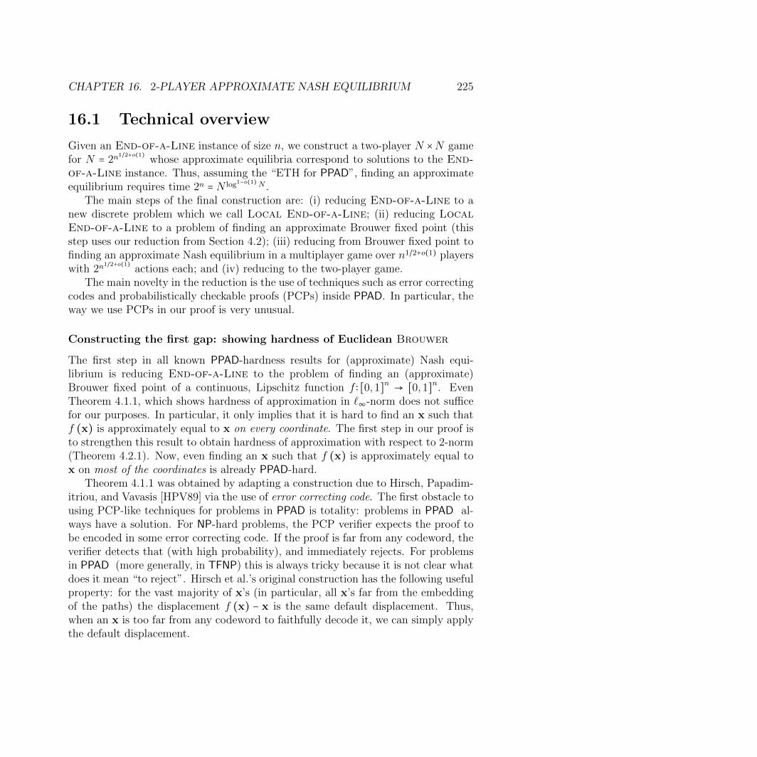
CHAPTER 16. 2-PLAYER APPROXIMATE NASH EQUILIBRIUM 225
16.1 Technical overview
Given an End-of-a-Line instance of size n, we construct a two-player N ×N gamefor N = 2n
1/2+o(1)whose approximate equilibria correspond to solutions to the End-
of-a-Line instance. Thus, assuming the “ETH for PPAD”, finding an approximateequilibrium requires time 2n = N log1−o(1)N .
The main steps of the final construction are: (i) reducing End-of-a-Line to anew discrete problem which we call Local End-of-a-Line; (ii) reducing LocalEnd-of-a-Line to a problem of finding an approximate Brouwer fixed point (thisstep uses our reduction from Section 4.2); (iii) reducing from Brouwer fixed point tofinding an approximate Nash equilibrium in a multiplayer game over n1/2+o(1) playerswith 2n
1/2+o(1)actions each; and (iv) reducing to the two-player game.
The main novelty in the reduction is the use of techniques such as error correctingcodes and probabilistically checkable proofs (PCPs) inside PPAD. In particular, theway we use PCPs in our proof is very unusual.
Constructing the first gap: showing hardness of Euclidean Brouwer
The first step in all known PPAD-hardness results for (approximate) Nash equi-librium is reducing End-of-a-Line to the problem of finding an (approximate)Brouwer fixed point of a continuous, Lipschitz function f ∶ [0,1]n → [0,1]n. EvenTheorem 4.1.1, which shows hardness of approximation in `∞-norm does not sufficefor our purposes. In particular, it only implies that it is hard to find an x such thatf (x) is approximately equal to x on every coordinate. The first step in our proof isto strengthen this result to obtain hardness of approximation with respect to 2-norm(Theorem 4.2.1). Now, even finding an x such that f (x) is approximately equal tox on most of the coordinates is already PPAD-hard.
Theorem 4.1.1 was obtained by adapting a construction due to Hirsch, Papadim-itriou, and Vavasis [HPV89] via the use of error correcting code. The first obstacle tousing PCP-like techniques for problems in PPAD is totality: problems in PPAD al-ways have a solution. For NP-hard problems, the PCP verifier expects the proof tobe encoded in some error correcting code. If the proof is far from any codeword, theverifier detects that (with high probability), and immediately rejects. For problemsin PPAD (more generally, in TFNP) this is always tricky because it is not clear whatdoes it mean “to reject”. Hirsch et al.’s original construction has the following usefulproperty: for the vast majority of x’s (in particular, all x’s far from the embeddingof the paths) the displacement f (x) − x is the same default displacement. Thus,when an x is too far from any codeword to faithfully decode it, we can simply applythe default displacement.

CHAPTER 16. 2-PLAYER APPROXIMATE NASH EQUILIBRIUM 226
The main challenge: locality.
Our ultimate goal is to construct a two-player game that simulates the Brouwerfunction from Theorem 4.2.1. This is done via an imitation gadget: Alice’s mixedstrategy induces a point x(A) ∈ [0,1]n; Bob’s strategy induces x(B) ∈ [0,1]n; Alicewants to minimize ∥x(A) − x(B)∥2, whereas Bob wants to minimize ∥f (x(A)) − x(B)∥2.Alice and Bob are both satisfied at a fixed point, where x(A) = x(B) = f (x(A)).(Recall also our construction of communicationally-hard games for Theorem 3.0.1.)
The main obstacle is that we want to incentivize Bob to minimize ∥f (x(A)) − x(B)∥2
via local constraints (payoffs - each depends on one pure strategy), while f (x(A))has a global dependency on Alice’s entire mixed strategy.
Our goal is thus to construct a hard Brouwer function that can be locally com-puted. How local does the computation need to be? In a game of size 2
√n×2
√n, each
strategy can faithfully store information about√n bits. Specifically, our construction
will be n1/2+o(1)-local.We haven’t yet defined exactly what it means for our construction to be “n1/2+o(1)-
local”; the exact formulation is quite cumbersome as the query access needs to bepartly adaptive, robust to noise, etc. Eventually (Section 16.4), we formalize the“locality” of our Brouwer function via a statement about multiplayer games. On ahigh level, however, our goal is to show that for any j ∈ 1, . . . , n, the j-th outputfj (x) can be approximately computed, with high probability, by accessing x at onlyn1/2+o(1) coordinates.
This is a good place to note that achieving any sense of “local computation” inour setting is surprising, even if we consider just the error correcting encoding forour Brouwer function: in order to maintain constant relative distance, an averagebit of the output must depend on a constant fraction of the input bits!
Local End-of-a-Line
In order to introduce locality, we go back to the End-of-a-Line problem. “Wishfulthinking”: imagine that we could replace the arbitrary predecessor and successorcircuits in End-of-a-Line with NC0 (constant depth and constant fan-in) circuitsSlocal, P local ∶ 0,1n → 0,1n, so that each output bit only depends on a constantnumber of input bits. Imagine further that we had the guarantee that for each input,the outputs of Slocal, P local differ from the input on just a constant number of bits.Additionally, it would be really nice if we had a succinct pointer that immediatelytold us which bits are about to be replaced. (We later call this succinct pointer thecounter, because it also cycles through its possible values in a fixed order.)

CHAPTER 16. 2-PLAYER APPROXIMATE NASH EQUILIBRIUM 227
Suppose all our wishes came true, and furthermore the hard Brouwer functionfrom Theorem 4.2.1 used a linear error correcting code. Then, we could use theencoding of the counter, henceforth C (u), to read only the bits that are about to bereplaced, and the inputs that determine the new values of those bits. Thus, usingonly local access to a tiny fraction of the bits (∣C (u)∣ + O (1)), we can constructa difference vector u − Slocal (u) (which is 0 almost everywhere). As we discussedabove, the encodings E (u) ,E (Slocal (u)) must differ on a constant fraction of thebits - but because the code is linear, we can also locally construct the differencevector E (u)−E (Slocal (u)) = E (u − (Slocal (u))). Given E (u)−E (Slocal (u)), wecan locally compute any bit of E (Slocal (u)) by accessing only the correspondingbit of E (u).
Back to reality: unfortunately we do not know of a reduction to such a restrictedvariant of End-of-a-Line. Surprisingly, we can almost do that. The problemLocal End-of-a-Line (formally defined in Section 16.2) satisfies all the guaranteesdefined above, is linear-time reducible from End-of-a-Line, but has one caveat: itis only defined on a strict subset V local of the discrete hypercube (V local ⊊ 0,1n).Verifying that a vertex belongs to V is quite easy - it can be done in AC0. Let ustake a brief break to acknowledge this new insight about the canonical problem ofPPAD:
Theorem 16.1.1. The predecessor and successor circuits of End-of-a-Line are,wlog, AC0 circuits.
The class AC0 is quite restricted, but the outputs of its circuits are not localfunctions of the inputs. Now, we want to represent u in a way that will make itpossible to locally determine whether u ∈ V local or not. To this end we augment thelinear error correcting encoding E (u) with a probabilistically checkable proof (PCP)π (u) of the statement (u ∈ V local).
Our holographic proof system
Some authors distinguish between PCPs and holographic proofs2: a PCP verifierhas unrestricted access to the instance, and queries the proof locally; whereas theholographic proof verifier has restricted, local access to both the proof and (an errorcorrecting encoding of) the instance. In this sense, what we actually want is aholographic proof.
2In a nutshell, PCPs or holographic proofs are proofs that can be verified “locally” (with highprobability) by reading only a small (random) portion of the proof; see e.g. [AB09, Chapter 18] formany more details.

CHAPTER 16. 2-PLAYER APPROXIMATE NASH EQUILIBRIUM 228
We construct a holographic proof system with some very unusual properties.We are able to achieve these properties thanks to our modest locality desideratum:n1/2+o(1), as opposed to the typical polylog (n) or O (1). We highlight here a few ofthese properties; see Section 16.3 for details.
• (Local proof construction) The most surprising property of our holographicproof system is that the proof π (u) can be constructed from local access to theencoding E (u). In particular, note that we can locally compute E (Slocal (u))because E (⋅) is linear - but π (⋅) is not. Once we obtain E (Slocal (u)), we canuse local proof construction to compute π (Slocal (u)) locally.
• (Very low random-bit complexity) Our verifier is only allowed to use(1/2 + o (1)) log2 n random bits - this is much lower even than the log2 n bitsnecessary to choose one entry at random. In related works, similar random-bitcomplexity was achieved by bundling the entries together via “birthday repe-tition”. To some extent, something similar happens here, but our locality isalready n1/2+o(1) so no bundling (or repetition) is necessary. To achieve nearlyoptimal random-bit complexity, we use λ-biased sets over large finite fieldstogether with the Sampling Lemma of Ben-Sasson et al. [Ben+03].
• (Tolerant verifier) Typically, a verifier must reject (with high probability)whenever the input is far from valid, but it is allowed to reject even if the inputis off by only one bit. Our verifier, however, is required to accept (with highprobability) inputs that are close to valid proofs. (This is related to the notionof “tolerant testing”, which was defined in [PRR06] and discussed in [GR05]for locally testable codes.)
• (Local decoding) We make explicit use of the property that our holographicproof system is also a locally decodable code. While the relations between PCPsand locally testable codes have been heavily explored (see e.g. Goldreich’s sur-vey [Gol10]), the connection to locally decodable codes is not as immediate.Nevertheless, related ideas of Locally Decode/Reject Codes [MR10] and de-codable PCP [DH13] have been used before in order to facilitate compositionof tests (our holographic proof system, in contrast, is essentially composition-free). Fortunately, as noted by [DH13] many constructions of PCPs are alreadyimplicitly locally decodable.
• (Robust everything) Ben-Sasson et al. [Ben+06] introduce a notion of ro-bust soundness, where on an invalid proof, the string read by the verifier mustbe far from any acceptable string. (Originally the requirement is far in expec-tation, but we want far with high probability.) Another way of looking at the

CHAPTER 16. 2-PLAYER APPROXIMATE NASH EQUILIBRIUM 229
same requirement, is that even if a malicious prover adaptively changes a smallfraction of the bits queried by the verifier, the test is still sound. In this sense,we require that all our guarantees, not just soundness, continue to hold (withhigh probability) even if a malicious entity adaptively changes a small fractionof the bits queried by the verifier.
How is local proof construction possible? At a high level, our holographic proofsystem expects an encoding of u as a low-degree t-variate polynomial, and a fewmore low-degree t-variate polynomials, that encode the proof of u ∈ V local. (Thisis essentially the standard “arithmetization”, dating back at least to [BF91; Sha92],although our construction is most directly inspired by [PS94; Spi95].) In our actualproof, t is a small super-constant, e.g. t ≜
√logn; but for our exposition here, let us
consider t = 2, i.e. we have bivariate polynomials.The most interesting part of the proof verification is testing that a certain low-
degree polynomial Ψ∶G2 → G, for some finite field G of size ∣G∣ = Θ (n1/2+o(1)), is iden-tically zero over all of F2, for some subset F ⊊ G of cardinality ∣F ∣ = ∣G∣ /polylog (n).This can be done by expecting the prover to provide the following low-degree poly-nomials:
Ψ′ (x, y) ≜ ∑fi∈F
Ψ (x, fi) yi
Ψ′′ (x, y) ≜ ∑fj∈F
Ψ′ (fj, y)xj.
Then, Ψ′′ (x, y) = ∑fi,fj∈F Ψ (fj, fi)xjyi is the zero polynomial if and only if Ψ isindeed identically zero over all of F2. Ψ (x, y) can be computed by accessing E (u)on just a constant number of entries. Thus, computing Ψ′ (x, y) requires Ψ (x, fi)for all fi ∈ F , so a total of Θ (n1/2+o(1)) queries to E (u). However, computing evenone entry of Ψ′′ (⋅) requires Ω (n) queries to E (u). The crucial observation is thatwe don’t actually need the prover to provide Ψ′′. Instead, it suffices that the proverprovide Ψ′, and the verifier checks that ∑fj∈F Ψ′ (fj, y)xj = 0 for sufficiently many(x, y).
Putting it all together via polymatrix games
The above arguments suffice to construct a hard Brouwer function (in the sense ofTheorem 4.2.1) that can be computed “n1/2+o(1)-locally”. We formalize this statementin terms of approximate Nash equilibria in a polymatrix game.
Definition 16.1.2 (Polymatrix games). In a polymatrix game, each pair of playerssimultaneously plays a separate two-player subgame. Every player has to play the

CHAPTER 16. 2-PLAYER APPROXIMATE NASH EQUILIBRIUM 230
same strategy in every two-player subgame, and her utility is the sum of her subgameutilities. The game is given in the form of the payoff matrix for each two-playersubgame.
We construct a bipartite polymatrix game between n1/2+o(1) players with 2n1/2+o(1)
actions each. By “bipartite”, we mean that each player on Alice’s side only interactswith players on Bob’s side and vice versa. The important term here is “polymatrix”:it means that when we compute the payoffs in each subgame, they can only dependon the n1/2+o(1) coordinates described by the two players’ strategies. It is in this sensethat we guarantee “local computation”.
The mixed strategy profile A of all the players on Alice’s side of the bipartitegame induces a vector x(A) ∈ [0,1]m, for some m = n1+o(1). The mixed strategyprofile B of all the players on Bob’s side induces a vector x(B) ∈ [0,1]m. Our maintechnical result is:
Proposition 16.1.3 (Informal). If all but an ε-fraction of the players play ε-optimally,
then ∥x(A) − x(B)∥2
2 = O (ε) and ∥f (x(A)) − x(B)∥2
2 = O (ε) .
Each player on Alice’s side corresponds to one of the PCP verifier’s random string.Her strategy corresponds to an assignment to the bits queried by the verifier giventhis random string. On Bob’s side, we consider a partition of 1, . . . ,m into n1/2+o(1)
tuples of n1/2+o(1) indices each. Each player on Bob’s side assigns values to one suchtuple.
On each two-player subgame, the player on Alice’s side is incentivized to imitatethe assignment of the player on Bob’s side on the few coordinates where they inter-sect. The player on Bob’s side, uses Alice’s strategy to locally compute fj (x(A)) ona few j’s in his (n1/2+o(1))-tuple of coordinates. This computation may be inaccurate,but we can guarantee that for most coordinates it is approximately correct most ofthe time.
From polymatrix to bimatrix
The final reduction from the polymatrix game to two-player game follows more orless from known techniques for hardness of Nash equilibria [Alt94; DGP09; BPR16].We let each of Alice and Bob control one side of the bipartite polymatrix game. Inparticular, each strategy in the two-player game corresponds to picking a player ofthe polymatrix game, and a strategy for that player. We add a gadget due to Althofer[Alt94] to guarantee that Alice and Bob mix approximately uniformly across all theirplayers. See Section 16.5 for details.

CHAPTER 16. 2-PLAYER APPROXIMATE NASH EQUILIBRIUM 231
16.1.1 The PCP Conjecture for PPAD
Recall our conjecture from Chapter 5:
Conjecture (PCP for PPAD; [BPR16]). There exist constants ε, δ > 0 such thatfinding an (ε, δ)-WeakNash in a bipartite, degree three polymatrix game with twoactions per player is PPAD-complete.
The main original motivation was an approach to prove our main theorem giventhis conjecture. As pointed out by [BPR16], it turns out that resolving this conjecturewould also have interesting consequences for relative approximations of two-playerNash equilibrium, as well as applications to inapproximability of market equilibrium.
More importantly, this question is interesting in its own right: how far can weextend the ideas from the PCP Theorem (for NP) to the wold of PPAD? ThePCP [r (n) , q (n)] characterization [AS98] is mainly concerned with two parame-ters: r (n), the number of random bits, and q (n), the number of bits read fromthe proof. A major tool in all proofs of the PCP Theorem is verifier composi-tion: in the work of Polishchuk and Spielman [PS94; Spi95], for example, it isfirst shown that NP ⊆ PCP [O (logn) , n1/2+o(1)], and then via composition it iseventually obtained that NP = PCP [O (logn) ,O (1)]. In some informal sense,one may think of our main technical result as something analogous3 to PPAD ⊆PCP [(1/2 + o (1)) log2 n,n
1/2+o(1)]. Furthermore, our techniques in Section 16.3 buildon many existing ideas from the PCP literature [Bab+91; PS94; Spi95; Ben+03;Ben+06] that have been used to show similar statements for NP. It is thus nat-ural to ask: is there a sense in which our “verifier” can be composed? can suchcomposition eventually resolve the PCP Conjecture for PPAD?
More generally, some of the tools we use here, even as simple as error correctingcodes, have been the basic building blocks in hardness of approximation for decades,yet to the best of our knowledge have not been used before for any problem in PPAD.We hope to see other applications of similar ideas in this regime.
16.1.2 Organization
In Section 16.2 we introduce the restricted variant Local End-of-a-Line and provethat it is also PPAD-complete. In Section 16.3 we construct our holographic proofsystem. In Section 16.4 we bring together ideas from Sections 4.2, 16.2, and 16.3 toprove our hardness for polymatrix games of subexponential size. Finally, in Section16.5 we reduce from polymatrix to two-player games.
3We stress that our analogy is very loose. For example, we are not aware of any formal extensionof PCP to function problems, and it is well known that NP ⊆ PCP [(1/2 + o (1)) log2 n,n
1/2+o(1)].

CHAPTER 16. 2-PLAYER APPROXIMATE NASH EQUILIBRIUM 232
Small constants
Our proof uses several arbitrary small constants that satisfy:
0 < εPrecision ≪ εNash ≪ δ ≪ h≪ εComplete ≪ εSound ≪ εDecode ≪ 1.
By ≪ we mean that we pick them such that εPrecision is arbitrarily smaller than anypolynomial in εNash, and εNash is arbitrarily smaller than any polynomial in δ, etc.Although their significance will be fully understood later in the paper, we brieflymention that εPrecision is the precision with which the players can specify real values;εNash is the approximation factor of Nash equilibrium in Proposition 16.3.1; δ and hare parameters of the Brouwer function construction; finally, εComplete, εSound, εDecode,are parameters of our holographic proof system.
16.2 End-of-a-Line with local computation
In this section we introduce a local variant of End-of-a-Line with very simplesuccessor and predecessor circuits.
Definition 16.2.1 (Local End-of-a-Line). The problem Local End-of-a-Line is similar to End-of-a-Line, but the graph is defined on a subset V local ⊆0,1n. The input consists of a membership circuit MV local ∶0,1n → 0,1 thatdetermines whether a string u ∈ 0,1n corresponds to a vertex of the graph (i.e.
MV local (u) =⎧⎪⎪⎨⎪⎪⎩
1 u ∈ V local
0 u ∉ V local), a special vertex u0 ∈ V local, and successor and prede-
cessor circuits Slocal, P local ∶ 0,1n → 0,1n with the promise that every outputbit depends only on a constant number of input bits. (I.e. Slocal and P local are inNC0.) Furthermore, we require that the outputs of Slocal and P local are identicalto the respective inputs, except at a constant number of coordinates. Similarly toEnd-of-a-Line, we are guaranteed that P local (u0) = u0 ≠ Slocal (u0).
The goal is to find an input u ∈ V local that satisfies any of the following:
• End-of-a-line: P local (Slocal (u)) ≠ u or Slocal (P local (u)) ≠ u ≠ u0; or
• Boundary conditions: Slocal (u) ∉ V local or P local (u) ∉ V local.
Notice that each vertex u ∈ V local, only defers from Slocal (u) and P local (u) ata constant number of bits, and the value of each of those only depends on a constantnumber of bits of u. We will refer to all those bits as the criticial bits of u, anddenote their cardinality qcritical.

CHAPTER 16. 2-PLAYER APPROXIMATE NASH EQUILIBRIUM 233
We now reduce End-of-a-Line to Local End-of-a-Line, proving that thelatter is PPAD-complete. In the following sections we use this reduction “white-box”, and revisit some of its specific properties.
Theorem 16.2.2. There is a linear-time reduction from End-of-a-Line to LocalEnd-of-a-Line.
Notice that there is a trivial reduction in the other direction: add self-loops toall strings not in V local.
Proof of Theorem 16.2.2. Given circuits S,P ∶0,1n → 0,1n, we construct newcircuits Slocal, P local ∶ 0,1m → 0,1m that satisfy Definition 16.2.1. We assumewlog that the circuits have fan-out 2 (otherwise, replace gates with larger fan-outswith a binary tree of equality gates; this only blows up the size of the circuit by aconstant factor). We set m = 4 (∣S∣ + ∣P ∣), where by ∣S∣ and ∣P ∣ we mean the numberof lines (i.e. number of inputs + number of logic gates) in each circuit, respectively.We think of the m bits as representing two copies of each circuit (S1, P1 and S2, P2),with each line represented by two bits, representing three possible states: value 0,value 1, and inactive.
The path begins with circuit S1 containing the computation from 0n to S (0n),and circuit P1 containing the reverse computation back to 0n; the lines of circuitsS2, P2 are inactive. This is the special vertex, u0.
Over the next n steps, the output bits of S1 are copied (one-by-one) to the inputbits of S2 (and the corresponding lines are activated). Over the next ∣S∣ − n steps,the values on the lines of S2 are updated -one-by-one, starting from the inputs andpropagating to the outputs in a fixed order- until all the output bits are activated andset to S (S (0n)). Then, over the next ∣P ∣ steps, the input of P2 is set to S (S (0n)),the values on the gates are updated (propagating in a fixed order from output toinput), and finally setting the output of P2 to S (0n).
Notice that so far, if we want to trace back a step (a.k.a. implement P local), wesimply need to deactivate the last activated line. We now start erasing values whengoing forward, but we must do so carefully so that we can reconstruct them whengoing backward. We proceed by deactivating the lines in S1: line by line, in reverseorder from outputs to inputs. Indeed, in order to go back we can reconstruct theoutput of any gate from its inputs. If we want to reconstruct an input to S1 - thisis no problem as it is saved as the output of P1. Once we finish deactivating S1, wedeactivate P1, also in reverse order. Notice again that the input to P1 is saved as theinput to S2 and output of P2. Now, we copy the values from S2 and P2 to S1 andP1 in the same order that we used to deactivate the lines, starting from the outputsof S1, to inputs, to outputs of P1, to inputs. Then we deactivate the lines in S2 and

CHAPTER 16. 2-PLAYER APPROXIMATE NASH EQUILIBRIUM 234
P2; again, we use the same order in which they were activated, starting from inputsof S2, to outputs, to inputs of P2, to outputs. So now we have S1 as a witness tothe computation of S (S (0n)) from S (0n) and P1 goes in the reverse order, whileall the lines of S2 and P2 are inactive.
We repeat the process from the last two paragraphs to find S (S (S (0n))), etc.We let V local to be the set of strings that correspond to a legal partial compu-
tation as described above. MV local verifies that a string corresponds to one of thefollowing scenarios:
• S1 holding the computation from some x ∈ 0,1n to S (x), P1 holding the com-putation from S (x) back to x, and S2 and P2 holding part of the computationfrom S (x) to S (S (x)) and back to S (x);
• S2 and P2 holding the computation from some x to S (x) and back to x, andP1 and S1 are in the process of erasing the computation from x to P (x) andback to x;
• S2 and P2 holding the computation from some x to S (x) and back to x, andS1 and P1 are in the process of copying it; or
• S1 and P1 holding the computation from some x to S (x) and back to x, areS2 and P2 in the process of erasing the same computation.
Notice that the joint active/inactive state of all the lines always belongs to one ofO (m) different states (that can be described by log2m +O (1) bits. Verifying thata string corresponds to one of the above scenarios is equivalent to checking that thejoint active/inactive state is valid, and that the values on all the lines satisfy all ofthe following local conditions:
• The i-th input of S1 is either inactive, equal to the i-th output of P1, or, if thelatter is inactive (during the copy phase), equal to the i-th input of S2.
• The i-th input of P1 is either inactive, equal to the i-th output of S1, or, if thelatter is inactive (during the erase phase), equal to the i-th input of S2.
• The output of every gate in S1, P1 is either inactive, equal to the gate appliedto its inputs, or, if either of the inputs is inactive (during the copy phase),equal to the respective line in S2, P2.
• The i-th input of S2 is either inactive, equal to the i-th output of P2, or, if thelatter is inactive (during the compute phase), equal to the i-th input of P2.

CHAPTER 16. 2-PLAYER APPROXIMATE NASH EQUILIBRIUM 235
• The i-th input of P2 is either inactive, equal to the i-th output of S2, or, if thelatter is inactive (during the erase phase), equal to the i-th input of P1.
• The output of every gate in S2, P2 is either inactive, equal to the gate appliedto its inputs, or, if either of the inputs is inactive (during the erase phase),equal to the respective line in S1, P1.
Notice that each line participates in at most three local constraints. Note also thateach of those conditions only depends on a constant number of bits so MV local , whichsimply needs to compute their AND, is in AC0 (this proves Theorem 16.1.1).
In every step a line is either activated or deactivated, so there are no fixed points;but fixed points of the original circuit lead to violations of the form P local (Slocal (u)) ≠u and Slocal (P local (u)) ≠ u ≠ u0. In particular, every solution to the new LocalEnd-of-a-Line instance corresponds to a valid solution to the original End-of-a-Line instance.
Also, notice that in every step we change at most two bits (and at least one),and deciding the next value of each bit can be done by looking only at a constantnumber of bits (conditioned on being a legal vertex in V local): which is the next lineto be activated/deactivated? if activated, what are the inputs to the correspondinggate?
16.2.1 The Local End-of-a-Line counter
Consider the instance produced in the reduction above. Notice that joint active/inactivestate of all the lines rotates amongO (m) possible vectors. I.e. there is a (logm +O (1))-bit vector, henceforth called the counter which describes precisely which lines shouldbe active. Furthermore, given the counter of some u ∈ V local, it is easy to com-pute the counter of Slocal (u) , i.e. we always know which line should be acti-vated/deactivated next - regardless of the values on the lines. Similarly, for allu ≠ u0 ∈ V local, it is also easy to compute the counter of P local (u). An additionaluseful property is that given the counter of u, we also know the coordinates of thecritical bits of u.
16.3 Holographic Proof
In this section we construct our holographic proof system for statements of theform u ∈ V local. Note that we use the term “verifier” loosely, as our verifier’sresponsibilities extend far beyond checking the validity of a proof - it is also expectedto perform local decoding, “local proof construction”, etc.

CHAPTER 16. 2-PLAYER APPROXIMATE NASH EQUILIBRIUM 236
Proposition 16.3.1. For sufficiently small constants εDecode ≫ εSound ≫ εComplete >0, the following holds. Fix any instance (Slocal, P local, V local) of Local End-of-a-Line, generated via the reduction in Section 16.2 from an instance (S,P ) End-of-a-Line. Given a vertex u ∈ V local, there is a polynomial time deterministicalgorithm that takes as input (S,P ) and u, and outputs a holographic proof Π (u) =(E (u) ,C (u) , π (u)) where:
• E (u) is an encoding of u with a linear error correcting code of constantrelative distance.
• C (u) is an encoding of the counter of u (with a good error correcting code).
• π (u) is a proof that u ∈ V local.
• Let n ≜ ∣u∣; then the total length of Π (u) is n1+o(1).
• Let t ≜√
logn (in particular, t = ω (1), but also t = o ( lognlog logn)). Let G be a
finite field of size O (n1/t+o(1)). E (u) and π (u) can be written as functions overdomain Gt. In particular, we can talk about accessing E (u), π (u), or Π (u) ata point g ∈ Gt. (C (u) is much shorter and the verifier reads it entirely.)
• There is a quasi-polynomial4 time probabilistic verifier such that:
– (Local access) The verifier’s access to Π (u) is restricted as follows:
∗ (Querying subspaces) The verifier reads no(1) axis-parallel (t/2)-dimensional subspaces of Π (u). Each subspace is defined by a re-striction of a (t/2)-tuple of coordinates. The tuple of coordinateswhich is restricted is always one of a constant number of possibili-ties (either 2, . . . , t/2 + 1, or the union of any two of: 1, . . . , t/4,t/4 + 1, . . . , t/2, t/2 + 1, . . . ,3t/4, and 3t/4 + 1, . . . , t). We de-note the union of all the subspaces read by the verifier GAll. It willbe useful to decompose GAll = GPCP∪GLTC∪Gcritical; another subsetof interest is GSample ⊂ GPCP.
∗ (Partially adaptive) GSample,GPCP,GLTC are chosen non-adaptively,i.e. they depend only on the verifier’s internal randomness. Gcritical
is a union of affine translations of a subspace that is also chosen non-adaptively, but the affine translations depend on C (u).
4The verifier of our holographic proof actually runs in polynomial time, except for the deran-domization of the construction of λ-biased sets. As we discuss in Section 2.7.3 this could also beobtained (with slightly worse parameters) in deterministic polynomial time, but quasi-polynomialtime suffices for the purpose of our main theorem.

CHAPTER 16. 2-PLAYER APPROXIMATE NASH EQUILIBRIUM 237
∗ (Randomness) The verifier uses only (1/2 + o (1)) log2 n bits of ran-domness to decide which subspaces to query.
∗ (Good Sample) For any function B∶Gt → [0,1], and any G ∈ GSample,GPCP,GLTC,Gcritical,with probability 1 − o (1) over the verifier’s randomness,
∣Eg∈G [B (g)] − Eh∈Gt [B (h)]∣ = o (1) .
– (Soundness) If the verifier is given a string Π′ which is εSound-far fromΠ (u) for every u ∈ V local, the verifier rejects with probability 1 − o (1).
∗ (Robust soundness) Furthermore, with probability 1−o (1), the bitsread by the verifier are ε2Sound-far from any string that would make theverifier accept. In other words, the verifier continues to reject withprobability 1 − o (1) even in the presence of an adaptive adversary,who observes the queries made by the verifier, and then corrupts anε2Sound/2-fraction of each of GPCP,GLTC.
– (Completeness) If the verifier is given access to a string Π that isεComplete-close to a valid Π (u) for some u ∈ V local, then the verifieraccepts with probability 1 − o (1).
∗ (Robust completeness) Furthermore, the verifier continues to ac-cept with probability at least 1−o (1) even in the presence of an adap-tive adversary, who observes the queries made by the verifier, andthen corrupts a
√εComplete-fraction of GPCP,GLTC.
– (Decoding) If the verifier is given access to a string Π that is εDecode-close to a valid Π (u) for some u ∈ V local:
∗ (Error-correction on a sample) With probability at least 1−o (1),the verifier correctly decodes the entries of E (u) and π (u) on GSample.In particular, with probability 1 − o (1), the verifier can estimate thedistance between Π and Π (u) to within an additive error of ±o (1).
∗ (Error-correction on the critical bits) The verifier can adap-tively decode and correct any qcritical-tuple of symbols from the proofwith success probability at least 1− o (1). Let Gcritical ⊂ Gt denote theunion of all O (∣G∣2) axis-parallel subspaces queried in this process.
∗ (Proof-construction) Given access as above to the counter C (u)and the linear code E (u) (but not to the proof π (u)), the verifier canoutput (with probability at least 1 − o (1)) the correct values of π (u)on GSample.

CHAPTER 16. 2-PLAYER APPROXIMATE NASH EQUILIBRIUM 238
∗ (Robust decoding) Both types of error-correction and the proof-construction continue to hold even in the presence of an adaptiveadversary, who observes the queries made by the verifier, and thencorrupts a
√εDecode-fraction of each of GSample,GPCP,GLTC,Gcritical.
The rest of this section is devoted to the proof of Proposition 16.3.1.
16.3.1 From Local End-of-a-Line to coloring graphs
Let t ≜√
logn. Set ` ≜ log2 nt−1 = Θ (
√logn), and `′ ≜ ` + c log logn for some sufficiently
large constant c. Let p (z) be an F2-irreducible polynomial of degree `′, and letG ≜ F2 [z] / ⟨p (z)⟩ denote the field of size 2`
′. We will focus our attention on a subset
F ⊂ G of polynomials (modulo p (z)) of degree `; notice that ∣G∣ / ∣F ∣ = poly logn.Let α be a generator of G, and let E ≜ 1, α, . . . , α5t`. We define the Extended
Shuffle-F-Exchange graph on F t−1×E to be the directed graph such that each vertex(x1, . . . , xt−1, αi) ∈ F t−1 × (E ∖ α5t`), has a static edge to vertex (x1, . . . , xt−1, αi+1),a shuffle edge to vertex (x2, . . . , xt−1, x1, αi+1), and ` exchange edges to all vertices ofthe form (x1 + [zj] , . . . , xt−1, αi+1), for every j ∈ 0, . . . , ` − 1. Here [zj] is the ele-ment of G representing the equivalence class zj + q (z)p (z) ∶ q (z) ∈ F2 [z]. Noticethat x ∈ F iff it can be written as x = ∑j∈S [zj] for some subset S ⊆ 0, . . . , ` − 1.In particular, for any (x1, . . . , xt−1) , (y1, . . . , yt−1) ∈ F t−1, the Extended Shuffle-F -Exchange graph contains a path of length (t − 1) (` + 1) from (x1, . . . , xt−1,1) to(y1, . . . , yt−1, α(t−1)(`+1)).
For each αi ∈ E , we call the set of vertices (x1, . . . , xt−1, αi) a layer; in particular,(x1, . . . , xt−1,1) form the first layer, and (x1, . . . , xt−1, α5t`) form the last layer.
We encode each vertex u ∈ V local as a partial coloring of the Extended Shuffle-F -Exchange graph, representing the assignments to the lines in the four circuitsS1, P1, S2, P2. Recall that ∣F ∣ = 2` = n1/(t−1). We associate each line of S1, P1, S2, P2
(including input, gates, and output lines) with a vector x ∈ F t−1 arbitrarily. Forthe first- and last-layer vertices (x,1) and (x, α5t`), we assign colors that representthe assignments (from 0,1,⊥, where ⊥ represents an inactive line) to the corre-sponding line. Recall from the “local conditions” in Section 16.2 that every line onlyparticipates in three constraints.
We would like the inputs to the line in (x1, . . . , xt−1, α5t`) to be propagated bythe Extended Shuffle-F -Exchange graph from the first layer. One important featureof the Extended Shuffle-F -Exchange graph is that we can do exactly that: By usingstandard packet-routing techniques, we can route the assignments from the first layerto the last layer so that every vertex on the way needs to remember at most threeassignments [Lei92, Theorem 3.16]. Fix one such routing. Our coloring now assigns

CHAPTER 16. 2-PLAYER APPROXIMATE NASH EQUILIBRIUM 239
the same color from 0,1,⊥× ⊥2to each of the corresponding vertices on the first
and last layers, and propagates this assignment through the middle layers accordingto the routing scheme; each vertex has a color in 0,1,⊥3
.It is important to note that the middle layers do not perform any computation
- they only copy symbols according to a fixed routing. In particular, if we changeone entry in the representation of Local End-of-a-Line vertex u, we can locallycompute the difference of the old and new assignments for every middle layer node,even if we don’t know the old assignment itself (which may correspond to up to threevalues routed through that node).
Notice that in order to verify that u ∈ V local, we need to check that the ac-tive/inactive pattern matches the counter, and the “local conditions”. Given acoloring of the Extended Shuffle-F -Exchange graph, checking the local conditionsreduces to checking that the color for each first-layer vertex is equal to the color onthe respective vertex on the last layer, and that the color of every vertex not in thefirst layer is computed correctly from its incoming neighbors.
16.3.2 Arithmetization
We now want to represent the verification of u ∈ V local as constraints on polynomialsover G (do not confuse with polynomials over F2!).
We represent each vertex u ∈ V local as two polynomials: Tu∶F t−1 × E → Cand Tcounter∶F t−1 → C, where C ⊂ F is a subset of F of constant size. For each(x1, . . . , xt−1, αi) ∈ F t−1 × E , we set Tu (x1, . . . , xt−1, αi) to be equal to the color as-signed to the respective vertex. Tcounter (x1, . . . , xt−1) is assigned 1 if the correspond-ing line should be active, and 0 otherwise. Additionally, we construct a polynomialTS,P ∶F t−1 × E → C′, for C ⊂ C′ ⊂ F of size ∣C′∣ = Θ (log3/2 n); TS,P (⋅) represents theinstance of End-of-a-Line: for each (x1, . . . , xt−1, α5t`) ∈ F t−1 × α5t`, it specifiesthe gate functionality, whereas for (x1, . . . , xt−1, αi) (i < 5t`) it specifies the routingthrough this vertex. Note that each vertex takes its inputs from at most 3 out ofΘ (
√logn) incoming edges.
Notice that Tu, Tcounter, TS,P are all polynomials of degree at most ∣F ∣ , ∣E ∣ in theirrespective variables. The verifier will expect low degree extensions of Tu, TS,P on allof Gt, and analogously for Tcounter over Gt−1.
In the following, keep in mind that Tcounter is constructed implicitly (once wedecode all log2 n + O (1) bits of the counter), and TS,P is part of the input of theproblem, so we only need to locally decode and verify the validity of Tu.
First, we construct a polynomial
Ψ (x) ≜ ψ (Tu (x)) ≜∏c∈C
(Tu (x) − c) , (16.1)
CHAPTER 16. 2-PLAYER APPROXIMATE NASH EQUILIBRIUM 240
such that ψ (Tu (x)) = 0 iff Tu (x) ∈ C.Similarly, we would like to construct a polynomial that verifies that the colors are
propagated correctly through the middle layers; for the last layer, it should also verifythat the gate functionality is implemented correctly. First, we describe the edges ofthe Extended Shuffle-F -Exchange graph with the following affine transformations:
ρStatic (x1, . . . , xt−1, αi+1) ≜ (x1, . . . , xt−1, α
i)ρShuffle (x1, . . . , xt−1, α
i+1) ≜ (xt−1, x1, . . . , xt−2, αi)
ρ0 (x1, . . . , xt−1, αi+1) ≜ (x1 + [z0] , . . . , xt−1, α
i)⋮
ρ`−1 (x1, . . . , xt−1, αi+1) ≜ (x1 + [z`−1] , . . . , xt−1, α
i)
(So each vertex x ∈ F t−1×(E ∖ 1) has incoming edges from ρStatic (x) , ρShuffle (x) , ρ0 (x) ,. . . , ρ`−1 (x).)
Now we can define a polynomial
Φ (x) ≜ φ (Tu (x) , Tu (ρStatic (x))Tu (ρShuffle (x)) , Tu (ρ0 (x)) , . . . , Tu (ρ`−1 (x)) , T(S,P ) (x)) ,(16.2)
where for x ∈ F t−1 × (E ∖ 1, α5t`), φ (⋯) = 0 iff the colors are propagated correctlyto the corresponding vertex, and for x ∈ F t × α5t`, φ (⋯) further checks that thegate functionality is implemented correctly.
Finally, we add a third polynomial over F t−1,
Ξ (x) ≜ ξ (Tu (x1, . . . , xt−1,1) , Tu (x1, . . . , xt−1, α5t`) , Tcounter (x1, . . . , xt−1)) , (16.3)
which is zero iff Tu (x1, . . . , xt−1,1) = Tu (x1, . . . , xt−1, α5t`) and the corresponding lineis active or inactive as dictated by Tcounter (x1, . . . , xt−1).
We now have that u ∈ V local is equivalent to AND of the following conditions:
• Values-in-domain: Ψ (x) = 0 for all x ∈ F t−1 × E ;
• Value-propagation and computation:Φ (x) = 0 for all x ∈ F t−1 × (E ∖ 1); and
• Active-vs-inactive: Ξ (x) = 0 for all x ∈ F t−1.
Notice also that ψ, ξ are constant total degree polynomials, whereas φ has totaldegree polylogn; thus Ψ,Φ,Ξ are of degrees ∣F ∣ ⋅polylogn, ∣E ∣ ⋅polylogn ≤ ∣G∣ /2 in theirrespective variables.

CHAPTER 16. 2-PLAYER APPROXIMATE NASH EQUILIBRIUM 241
16.3.3 PCP
Our verifier should test that Ψ,Φ,Ξ are zero everywhere on the respective domains(F t−1×E ,F t−1× (E ∖ 1) ,F t−1). We describe the test for Ψ; the corresponding testsfor Φ and Ξ follow analogously.
In order to test that Ψ (x) is zero over all of F t−1 × E , consider the followingpolynomials:
Ψ′ (x1, . . . , xt−1, α
j) ≜ ∑fit/2+1
,...,fit−1∈F
j′∈1,...,5t`
Ψ (x1, . . . , xt/2, fit/2+1, . . . , fit−1 , α
j′
)t−1
∏k=t/2+1
xik−1k ⋅ (αj)j
′
(16.4)
Ψ′′ (x1, . . . , xt−1, α
j) ≜ ∑fi1 ,...,fit/2∈F
Ψ′ (fi1 , . . . , fit/2 , xt/2+1, . . . , xt−1, α
j)t/2∏k=1
xik−1k . (16.5)
In particular, observe that
Ψ′′ (x1, . . . , xt−1, α
j) = ∑fi1
,...,fit−1∈F
j′∈1,...,5t`
Ψ (fi1 , . . . , fit−1 , αj′) ⋅
t−1
∏k=1
xik−1k ⋅ (αj)j
′
.
The main point of this construction is that Ψ′′
is the zero polynomial if and onlyif Ψ (x) = 0 for every x ∈ F t−1×E . Now, by definition, Ψ
′′has degrees at most ∣F ∣ , ∣E ∣
in each variable, respectively, so it suffices to test that it is indeed zero at one randompoint from Gt.
The verifier should also ensure that Ψ′
and Ψ′′
are constructed correctly. This isdone by picking a uniformly random x ∈ Gt and verifying that (16.4) and(16.5) hold.If Ψ is constructed correctly, then Ψ
′also has low degrees in each variable (compared
to ∣G∣), so it suffices to test on a single x ∈ Gt. Similarly, the verifier should also checkthat Ψ is constructed correctly as in (16.1); thanks to the low-degree guarantee, asingle x ∈ Gt suffices here as well.
Notice that the verifier does not need to receive Ψ′′
explicitly. (This is cru-cial later for the proof construction!) Testing that Ψ
′′is constructed correctly at
(x1, . . . , xt−1, αj) and that it is zero at the same point is equivalent to simply testingthat
∑fi1 ,...,fit/2∈F
Ψ′ (fi1 , . . . , fit/2 , xt/2+1, . . . , xt−1, α
j)t/2∏k=1
xik−1k = 0. (16.6)
We also need to test that all polynomials are indeed low degree. We do this later,in Subsection 16.3.7.
CHAPTER 16. 2-PLAYER APPROXIMATE NASH EQUILIBRIUM 242
Define and test Φ′,Ξ
′analogously to Ψ
′. We conclude that if Tu,Ψ,Φ,Ξ,Ψ
′,Φ
′,Ξ
′
are all indeed of low degrees as promised and the verifier accepts with probabilitygreater than ε, then Tu, Tcounter represent a real vertex u ∈ V local. Notice that all ofour tests choose x ∈ Gt/2 with uniform marginal probabilities.
For simplicity of notation, we henceforth treat Ξ (⋅) as t-variate polynomial (withthe t-th variable being a dummy variable).
16.3.4 The final encoding
Our proof Π (u) consists of the following strings.
• C (u) consists of a good encoding of the “counter” of u. (Notice that we requirea succinct encoding that can be fully decoded, and then the entire Tcounter canbe computed locally.)
• E (u) consists of the polynomial Tu∶Gt → G.
• π (u) consists of the polynomials Ψ,Ψ′,Φ,Φ′,Ξ,Ξ
′ ∶Gt → G.
Although they have different lengths (in particular, C (u) is much shorter), we thinkof them as having equal “weights”, i.e. we allow only a constant fraction of errors ineach. Also, we think of symbols in larger alphabets as encoded with a good binaryerror correcting code.
16.3.5 Local decoding and error correction
When a typical PCP verifier is given a proof that is wrong even at a single bit,it is already allowed to reject the proof. For our purpose, we want a more lenientverifier that, when given a proof that is wrong at a small fraction of the bits, correctsthose bits and accepts. Furthermore, we want to ensure that our verifier only usesvery little randomness: only (1/2 + o (1)) log2 n random bits. A second goal of thissubsection is to establish the desideratum that the verifier can adaptively decode anarbitrary qcritical-tuple of entries from the proof.
We describe how to locally decode and correct Ψ; Tu,Ψ′,Φ,Ξ,Φ
′,Ξ
′follow with
minor modifications, whereas the counter has a succinct representation and can befully decoded. Specifically, the verifier needs to decode Ψ in order to test (16.1),(16.4). For (16.1) the verifier only needs to decode Ψ at one uniformly randompoint, so this is the easy case. For (16.4), the verifier wants to decode an entireaxis-parallel (t/2)-dimensional affine subspace, Q(x1,...,xt/2) ≜ (x1, . . . , xt/2) × Gt/2,
for a uniformly random choice of (x1, . . . , xt/2) ∈ Gt/2.

CHAPTER 16. 2-PLAYER APPROXIMATE NASH EQUILIBRIUM 243
Let S ⊂ Gt/2 be a (1/ (t2 log ∣G∣))-biased set of cardinality ∣S∣ = poly (t, log ∣G∣) (asguaranteed by Section 2.7.3). We pick a uniformly random x = (x1, . . . , xt/2) ∈ Gt/2,
and a uniformly random y = (y1, . . . , yt/2) ∈ S. We then consider the (t/2 + 1)-dimensional affine subspace Rx,y ≜ ⋃β∈GQ(x+βy). If Ψ is O (εDecode)-close to Ψ, we
have by Lemma 2.7.5 that with probability 1 − o (1), the restriction of Ψ to Rx,y,denoted Ψ ∣Rx,y , is also O (εDecode)-close to Ψ ∣Rx,y . Whenever this is the case, theverifier correctly decodes Ψ on Rx,y.
Notice that so far, our verifier queries ∣G∣t/2+1 = n1/2+o(1) symbols, and useslog2 ∣Gt/2∣ + log2 ∣S∣ = (1/2 + o (1)) log2 n random bits.
The local decoding for Tu,Ψ′,Φ,Ξ,Φ
′,Ξ
′follows with minor modifications which
we now describe. Notice that we can reuse the same random bits from the decodingof Ψ to decode each of the other polynomials. For (16.5) the verifier wants to decodeΨ
′(equivalently for Φ
′,Ξ
′) on a subspace that fixes the second half of the coordinates,
Q′
(xt/2+1,...,xt)≜ Gt/2 × (xt/2+1, . . . , xt).
For (16.1) and (16.3), the verifier also needs to decode one or two entries ofTu, but this is no harder than decoding an entire plane. For (16.2), there is somesubtlety: Φ (x) is a function of the values of Tu on a super-constant number (` + 3 =Θ (
√logn)) of points x, ρStatic (x) , ρShuffle (x) , ρ0 (x) , . . . , ρ`−1 (x). Observe that
x, ρStatic (x) , ρ0 (x) , . . . , ρ`−1 (x) all belong to the same (t/2)-dimensional subspace(only the first and last coordinates change); thus we only need to apply subspace-decoding twice.
Notice that our decoding mechanism also suffices to locally correct errors (withprobability at least (1 − o (1)), and assuming that we start with a function that isclose to low-degrees). Furthermore, by Lemma 2.7.5, the distance ∣Ψ ∣Rx,y −Ψ ∣Rx,y ∣is within ±o (1) of the global distance ∣Ψ −Ψ∣. Handling the rest of the polynomials
as described in the previous paragraphs, we can thus estimate ∣Π ∣E,π −Π (u) ∣E,π∣to within ±o (1); for the bits that correspond to the counter, we can compute thedistance exactly.
Decoding a particular subspace
Above, we described how to locally decode a random subspace. Suppose instead thatwe want to locally decode Ψ ∣Q(w1,...,wt/2)
for some particular w ∈ Gt/2 (specifically,
when Q(w1,...,wt/2) contains information about one of the critical bits). Since we did
not waste any random bits on picking w, we can afford to pick y uniformly from all ofGt/2. On the other hand, since w is arbitrary, there may still be an Θ (εDecode) chancethat ∣Ψ ∣Rw,y −Ψ ∣Rw,y ∣ is too large (> 1/2) to guarantee correct decoding. Instead, we

CHAPTER 16. 2-PLAYER APPROXIMATE NASH EQUILIBRIUM 244
pick a third vector z ∈ S, and query Ψ on the (t/2 + 2)-dimensional affine subspacePw,y,z ≜ ⋃β,γ∈GQ(w+β(y+γz)); notice that Pw,y,z ≜ ⋃γ∈G Rw,y+γz. In expectation, for
each (y + γz)’s, the restriction Ψ ∣Rw,y+γz is at distance at most O (εDecode) fromΨ ∣Rw,y+γz . Therefore, by Lemma 2.7.5, with probability 1 − o (1), we have that
∣Ψ ∣Pw,y,z −Ψ ∣Pw,y,z ∣ = O (εDecode).
16.3.6 Local proof-construction
We now want to establish the following unusual property of our holographic proofscheme: we can, with high probability, locally construct any subspace Q(x1,...,xt/2) of
the proof π (u), by reading only a small part of the encoding E (u) (in particular, weneed to decode a constant number of (t/2 + 1)-dimensional subspaces from E (u)).Here, it is important that Q(x1,...,xt/2) is defined via a restriction of the first t/2coordinates, but we assume access to decoded subspaces of E (u) with restriction ofany (t/2)-tuple of coordinates.
Recall that in order to compute Ψ (x) or Ξ (x), it suffices to know the values of Tuat a constant number of locations ((16.1) and (16.3)), so here this property triviallyholds. For Φ (x), we need to know Tu at Θ (
√logn) locations (16.2); however, as
we argue in Subsection 16.3.5, they belong to two axis-parallel subspaces, so it againsuffices to decode Tu on a constant number of subspaces.
In order to compute Ψ′ (x) ,Φ′ (x) ,Ξ′ (x), we need to correctly decode the val-
ues of Ψ,Φ,Ξ on (almost) an entire axis-parallel subspace Q(x1,...,xt/2). The values of
Ψ,Φ,Ξ are not given as part of E (u), but (as we argued in the previous paragraph),we can reconstruct them from Tu. Specifically, in order to know the values of Ψ orΞ on Q(x1,...,xt/2), we simply need to decode Tu on Q(x1,...,xt/2). In order to construct
Φ on an entire subspace, observe that for every (x1, . . . , xt/2, fit/2+1, . . . , fit−1 , α
j) ∈Q(x1,...,xt/2), all the vectors ρStatic (x1, . . . , xt/2, fit/2+1
, . . . , fit−1 , αj) , ρ0 (x1, . . . , xt/2, fit/2+1
, . . . , fit−1 , αj) , . . . ,
ρ`−1 (x1, . . . , xt/2, fit/2+1, . . . , fit−1 , α
j) belong to the same subspace Q(x1,...,xt/2). Fur-
thermore, all the vectors ρShuffle (x1, . . . , xt/2, fit/2+1, . . . , fit−1 , α
j) = (fit−1 , x1, . . . , xt/2, fit/2+1, . . . , fit−2 , α
j)belong to the subspace QShuffle
(x1,...,xt/2)≜ G × (x1, . . . , xt/2)×Gt/2−1. Therefore the value of
Φ′ (x) can also be computed from the values of Tu on a constant number of subspaces.
16.3.7 Local robust testing
So far, we assumed that we are given functions that are low degree (Subsection16.3.3), or approximately low degree (Subsection 16.3.5). However, we must verifythat this is indeed the case.
CHAPTER 16. 2-PLAYER APPROXIMATE NASH EQUILIBRIUM 245
We will use results for locally testing tensor codes [Vid15]. In order to describethem, let us briefly introduce some minimal background and notation. Given linearcodes C1,C2 with respective generator matrices M1,M2, their tensor product, denotedC1 ⊗C2 is the linear code generated by the tensor product of the matrices M1 ⊗M2.We say that C1⊗C2 is a tensor code. In general, we can talk about the tensor productof k codes, C1 ⊗ ⋅ ⋅ ⋅ ⊗ Ck, which is defined recursively. We say that C1 ⊗ ⋅ ⋅ ⋅ ⊗ Ck isthe k-th power of C (denoted Ck), if Ci = C for all i ∈ [k]. In our case, for example,the code C of all (∣G∣ /2)-individual degrees polynomials T ∶Gt → G is the t-th powerof the code of all (∣G∣ /2)-degree polynomials t∶G → G.
Alternatively, we can think of any product code as a function from some productdomain to some range. The (axis-parallel) hyperplane tester picks a uniformly ran-dom index i ∈ [k], and a uniformly random value vi from the i-th domain. It readsthe assignment of the function for all vectors that have vi in their i-th coordinate, andtests whether they form (or are close to) a codeword from C1⊗⋅ ⋅ ⋅⊗Ci−1⊗Ci+1⊗⋅ ⋅ ⋅⊗Ck.Going back to our setting, this could mean selecting a random i ∈ 1, . . . , t, and arandom value vi ∈ G; reading T (x) for all x such that xi = vi, and verifying that therestricted (t − 1)-variate function is close to a low degrees polynomial.
To optimize query complexity, it will be more convenient for us to think of thecode of (t/4)-variate (∣G∣ /2)-individual degrees polynomials Tt/4∶Gt/4 → G, henceforth
denoted C1/4. The code C can now be written C = (C1/4)4. The hyperplane tester now
chooses a random i ∈ 1,2,3,4 and a random value vi ∈ Gt/4, and reads T (x) for allx whose restriction to the i-th (t/4)-tuple of coordinates is equal to vi.
We can now apply the following theorem due to Viderman [Vid15]:
Theorem 16.3.2. [Vid15, Theorem 4.4] Let C = C1⊗⋅ ⋅ ⋅⊗Ck be the tensor product ofk > 2 linear codes of relative distances δ1, . . . , δk. Let M be a string which is ε-far fromthe tensor code C. Then the restriction of M to a random hyperplane drawn from the
above distribution is, in expectation, at least (ε ⋅ ∏kj=1 δj
2k2 )-far from the restricted code
C1 ⊗ ⋅ ⋅ ⋅ ⊗Ci−1 ⊗Ci+1 ⊗ ⋅ ⋅ ⋅ ⊗Ck.
Let S1/4 ⊂ Gt/4 be a (1/ (t2 log ∣G∣))-biased set of cardinality ∣S1/4∣ = poly (t, log ∣G∣)(for example, take the restriction of each y ⊂ S to its first t/4 entries). Sample
x ∈ Gt/4 and y ∈ S1/4 uniformly at random. Run the hyperplane tester for (C1/4)4
on each alleged polynomial 4 ∣G∣ times, taking all the possibilities for i ∈ 1,2,3,4and vi = (x + βy) for all β ∈ G. By Theorem 16.3.2, if the polynomial is εSound-far
from (C1/4)4, then the expected distance on each of the 4 ∣G∣ tests is (εSound ⋅ ∏
kj=1 δj
2k2 ) =εSound/512 (since k = 4 and δj ≥ 1/2). By Lemma 2.7.5, the average over all the testsis, with probability 1 − o (1), within ±o (1) of this expectation.

CHAPTER 16. 2-PLAYER APPROXIMATE NASH EQUILIBRIUM 246
So far the tester requires (1/4 + o (1)) log2 n random bits to sample a hyperplane,but has prohibitively high query complexity: n3/4+o(1). In order to drive down thequery complexity, we can recurse on the test using fresh (1/4 + o (1)) log2 n random
bits: we re-partition (C1/4)3
as a tensor product of three linear codes, and reapplyViderman’s theorem. Our query complexity is now n1/2+o(1), the total random-bits
complexity is (1/2 + o (1)) log2 n, and the robustness guarantee is (εSound ⋅ 2−4
2⋅42 ⋅ 2−3
2⋅32)−o (1) > εSound/105.
Finally, our tester accepts iff the average distance across all (t/2)-dimensional sub-spaces from the nearest low-degrees polynomial is less than 2
√εComplete < εSound/ (2 ⋅ 105).
Thus our tester accepts with high probability whenever Ψ is εComplete-close to thetrue Ψ, and rejects with high probability whenever Ψ is εSound-far from any lowdegrees polynomial. (Testing Tu, Φ, Ξ, Ψ
′ , Φ′ , Ξ′ follows analogously.)
16.3.8 Summary
The verifier, on input Π = (E, C, π), does the following.
Randomness
In a preprocessing step, the verifier fixes in advance a (1/ (t2 log ∣G∣))-biased set S ofcardinality ∣S∣ = poly (t, log ∣G∣). Let S1/4 denote the restriction of S to the first t/4coordinates.
The tester then:
• draws x uniformly at random from Gt/2, and y uniformly at random from S;and
• reusing the same randomness, draws x1,x2 ∈ Gt/4 and y1,y2 ∈ S1/4.
Queries
The verifier reads Tu on all vectors z ∈ Gt such that one of (z1, . . . , zt/2) , (z2, . . . zt/2+1)is of the form (x + βy) for some β ∈ G. It also reads Ψ, Φ, Ξ, Ψ′ , Φ′ , Ξ′on all z ∈ Gt suchthat (z1, . . . zt/2) = (x + βy) for some β ∈ G (denote those vectors Rx,y). Similarly, it
also reads Ψ′, Φ
′, and Ξ
′on all z ∈ Gt such that (zt/2+1, . . . , zt) = (x + βy) (denote
those vectors R′x,y). The union of all those subspaces (i.e. Rx,y ∪R′
x,y) forms GPCP,while GSample ≜ Rx,y.
For each choice of i1 ≠ i2 ∈ 1,2,3,4 and each β1, β2 ∈ G, the verifier reads eachpolynomial on all vectors z ∈ Gt such that the i1-th (t/4)-tuple of z is equal to

CHAPTER 16. 2-PLAYER APPROXIMATE NASH EQUILIBRIUM 247
x1 +β1y1, and the i2-th (t/4)-tuple of z is equal to x2+β2y2 . The union of all thosesubspaces forms GLTC.
Finally, the verifier also reads the entire encoding C (u) of the counter of u. GivenC (u), the verifier also picks qcritical vectors w1, . . . ,wqcritical ∈ Gt/2 that correspondto each of the critical bits, and reads Tu on all vectors z ∈ Gt such that (z1, . . . , zt/2) =(wi + β (x + βy)) for some β, γ ∈ G and i ∈ 1, . . . , qcritical. Those are Gcritical.
Test
The verifier uses the hyperplane tester from Subsection 16.3.7 to verify that all thepolynomials are indeed close to low-degree polynomials. (If not, it suffices to returnan error message and abort.)
Correct & decode
For each subspace queried, the verifier finds the unique low-degree polynomialsTu,Ψ,Φ,Ξ,Ψ
′,Φ
′,Ξ
′that are close to the values read.
Verify
The verifier checks that the corrected polynomials Tu,Ψ,Φ,Ξ,Ψ′,Φ
′,Ξ
′satisfy (16.1),
(16.2), (16.3), and (16.4) on all of Rx,y. It also checks that (16.6) (and its analoguesfor Φ
′,Ξ
′) are satisfied on all of R
′x,y.
Estimate distance
The verifier also computes the hamming distance between the values of Tu, Ψ, Φ, Ξ, Ψ′ , Φ′ , Ξ′
and Tu,Ψ,Φ,Ξ,Ψ′,Φ
′,Ξ
′on Rx,y.
Extrapolate
Given C (u), the verifier can locally reconstruct C (Slocal (u)). Additionally, afterthe verifier decoded the values of Tu at the critical bits, it also knows the currentand new values of all the entries that change between u and Slocal (u). Since E (⋅)is a linear encoding, the verifier can also completely construct the difference vectorE (Slocal (u))−E (u). In other words, given the value of Tu (x) for any x, the verifiercan locally compute TSlocal(u) (x).
The verifier can use the ideas from Subsection (16.3.6) to also construct the valuesof all the polynomials (Ψ,Φ,Ξ,Ψ
′,Φ
′,Ξ
′) for Slocal (u), on all of Rx,y.

CHAPTER 16. 2-PLAYER APPROXIMATE NASH EQUILIBRIUM 248
For P local (u), the verifier must first check that u is not the special vertex u0.This is easy to do since Tu and the respective Tu0 are both low degree polynomialsand must differ (if u ≠ u0) on a constant fraction of their entries. If indeed u ≠ u0,recovering information about P local (u) is completely analogous to the procedure forSlocal (u). Otherwise, we simply have P local (u0) = u0.
16.4 Polymatrix WeakNash
In this section we prove our main technical result:
Theorem 16.4.1. There exists a constant εNash > 0, such that there is a 2n1/2+o(1)
-timereduction from End-of-a-Line to finding an (εNash, εNash)-Well-Supported-WeakNashof a complete bipartite polymatrix game between n1/2+o(1) players with 2n
1/2+o(1)actions
each; the payoffs in each bimatrix subgame are in [0,1/nB] , [0,1/nA], where nA, nBdenote the number of players on each side of the bipartite graph.
We construct a subexponential polymatrix game that implements a variant ofthe hard Brouwer function constructed in Section 4.2. The new Brouwer function isvery similar, but we make the following modifications:
• We use the vertices of a Local End-of-a-Line instance instead of End-of-a-Line.
• Instead of encoding each Local End-of-a-Line vertex u with an arbitraryerror correcting code, the Brouwer vertices correspond to the holographic proofsΠ (u) from Section 16.3.
• For convenience of notation, instead of maintaining m coordinates (which weexpect to be identical anyway), for each of the auxiliary compute-vs-copy bitand the special direction, we keep just one coordinate for each, but give eacha constant relative weight.
• In particular, the “first” Brouwer line segment goes from z2 ≜ (Π (u0) ,Π (u0) ,0,2)to (Π (u0) ,Π (u0) ,0,0).
The rest proof proceeds as follows: In Subsection 16.4.1, we define the strategy spacefor the players and relate it to the holographic proof system from Section 16.3. InSubsection 16.4.2 we introduce some important notation used throughout this sec-tion. In the next two subsections (16.4.3 and 16.4.4) we define the players’ payoffs,

CHAPTER 16. 2-PLAYER APPROXIMATE NASH EQUILIBRIUM 249
and implement an imitation gadget, assuming that the Brouwer function f can be lo-cally computed. In Subsection 16.4.5, we translate the PCP guarantees from Propo-sition 16.3.1 to guarantees about approximate equilibria of our polymatrix game.This completes the setup of the argument. The rest of this section (Subsections16.4.6-16.4.9) shows that we can indeed locally compute f in the different regionswhere it is defined (outside the picture, close to a Brouwer line segment, etc.).
16.4.1 Players and strategies
Let RPCP denote the set of random strings used by the PCP verifier in Proposition16.3.1. For each r ∈ RPCP we construct a player (A, r) on one side of the bipartitegame. On the opposite side, we construct a player (B,q) for every q ∈ Gt/2. We referto the respective sides of the bipartite game as Alice’s players and Bob’s players. (InSection 16.5 we will construct a bimatrix game between Alice and Bob where eachplayer “controls” the vertices on her or his side of the polymatrix game.)
Each player has (3/εPrecision + 1)n1/2+o(1)+2
actions. We think of each action as anordered tuple of:
• two vectors in [−1,2]n1/2+o(1)
, where the interval [−1,2] is discretized into −1,−1 + εPrecision, . . . ,2 − εPrecision,2;and
• two more variables in [−1,2].
Recall that each Brouwer vertex corresponds to a pair (u, v) of either identical orconsecutive vertices from the Local End-of-a-Line instance. For player (A, r),the two vectors allegedly correspond to bits read from two holographic proofs (a-laSection 16.3) (Π (u) ,Π (v)) by the PCP verifier with random string r. For player(B,q) the vectors represent (a binary encoding of) the counters C (u) ,C (v), andthe entries of E (u) , π (u) ,E (v) , π (v) on a (t/2)-dimensional subspace G(B,q) ⊂ Gtto be specified below.
The additional two variables represent the compute-vs-copy bit and the specialdirection.
In addition to the assignments described above, each player on Alice’s side has
an additional choice among (3/εPrecision + 1)n1/2+o(1)
actions. These additional actionsallegedly correspond to 2qcritical (affine, (t/2 + 2)-dimensional) subspaces from whichwe can decode the qcritical critical bits of each of the vertices. (We know which entriesare represented by reading the “counter” part of the proof.)
CHAPTER 16. 2-PLAYER APPROXIMATE NASH EQUILIBRIUM 250
Bob’s subspace G(B,q)
Let G(A,r)All ⊂ Gt denote the set of entries of E (⋅) , π (⋅) read by the PCP verifier with
random string r. Recall that the PCP verifier picks a set of (t/2)-dimensional axis-parallel affine subspaces; each subspace is an affine shift of a linear subspace, spannedby one of a constant number of (t/2)-tuples of standard basis vectors. We pick G(B,q)
so that it is spanned by vectors that are linearly independent of all those tuples. Inparticular, G(B,q) intersects each of (A, r)’s subspaces at exactly one point.
For any (t/2)-tuple of standard basis vectors of Gt, a uniformly random (t/2)-tuple of new vectors in Gt completes it to a basis with high probability. To seethis, consider adding the new vectors one by one; at each step, there is at least a(1 − 1/ ∣G∣)-probability that it is linearly independent of the previously chosen vectors;the claim follows by union bound and t = o (∣G∣). Therefore, a random (t/2)-tupleof vectors will also, with high probability, be simultaneously linearly independent ofeach of the relevant tuples of standard basis vectors. Fix any such a (t/2)-tuple (thereare also efficient ways to deterministically find such a tuple, but in quasi-polynomialtime we can simply brute-force enumerate through all tuples).
Finally, we let G(B,0t/2) be the linear subspace spanned by those vectors; forgeneral q ∈ Gt/2, we let G(B,q) be the same subspace shifted by (q,0t/2).
16.4.2 Notation
We introduce some necessary additional notation for formally handling vectors inthis section. The notation for (A, r)’s assignment to the critical bits is analogous inspirit but more subtle to formalize; we come back to it to Subsection 16.4.3.
Definition 16.4.2. We say that a player is happy if every strategy on her supportis εNash-optimal.
Rounding For x ∈ R, let ν (x) ≜⎧⎪⎪⎨⎪⎪⎩
1 x > 1/20 otherwise
denote the rounding of x to 0,1;
for x ∈ Rn, we compute ν (x) coordinate-wise.
Coordinates Let M ≜ 1, . . . ,2m + 2 denote the set of all coordinates. We par-tition M into: M1 ≜ 1, . . . ,m (the first proof), M2 ≜ m + 1, . . . ,2m (the secondproof), M3 ≜ 2m + 1 (the Compute-vs-Copy bit), and M4 ≜ 2m + 2 (the specialdirection). We will also use the abbreviations M1,2 ≜M1 ∪M2 and M3,4 ≜M3 ∪M4.
Fix some player (A, r) on Alice’s side; we further detail (A, r)’s strategy space as
follows. Let G(A,r)Sample,G
(A,r)PCP ,G
(A,r)LTC ⊂ Gt denote the sets of entries of E (⋅) , π (⋅) read by

CHAPTER 16. 2-PLAYER APPROXIMATE NASH EQUILIBRIUM 251
the PCP verifier with random string r from the alleged proofs. Let I(A,r)Sample, I
(A,r)PCP , I
(A,r)LTC ⊂
M1,2 denote the indices of the corresponding bits, respectively. For player (B,q) onBob’s side, let I(B,q) ⊂ M1,2 denote the indices of the bits corresponding to G(B,q).We also let K ⊂ M1,2 (K for Kounter) denote the set of indices that correspond tothe encodings of counters in both proofs. (Notice that K is the same for every playeron both sides.)
Finally we will be particularly interested in the following sets:
J(A,r) ≜ K ∪ I(A,r)Sample ∪M3,4
J(B,q) ≜ K ∪ I(B,q) ∪M3,4.
Partial vectors Player (A, r)’s strategy a naturally corresponds to a partial vector
x(a)All ∈ ([−1,2] ∪ ⊥)M . For i ∈ K ∪ I(A,r)PCP ∪ I(A,r)LTC ∪M3,4, we set the i-th coordinate
of x(a)All to the value that a assigns to the corresponding coordinate; for all other i’s,
we let x(a)All ∣i≜⊥.
In particular we are interested in the partial vector x(a) ∈ ([−1,2] ∪ ⊥)M thatdescribes (A, r)’s partial assignment to J(A,r). For i ∈ J(A,r), we set the i-th coordi-nate of x(a) to the value that a assigns to the corresponding coordinate; for all otheri’s, we let x(a) ∣i≜⊥.
For action b taken by player (B,q), we can simply define one partial vectorx(b) ∈ ([−1,2] ∪ ⊥)M , where x(b) ∣i≜⊥ for i ∉ J(B,q).
Partial norms All norms in this section are 2-norm: we henceforth drop the2 subscript from ∥⋅∥2. Instead, we will use the subscript to denote the subset ofcoordinates over which we want to compute the norm. For example,
∥x∥2K ≜ Ei∈K [x2
i ] .
In fact, we are often interested in expectation with respect to a non-uniform distri-bution; for example:
∥x∥2J(A,r) ≜ 1
4Ei∈I(A,r)Sample
[x2i ] +
1
4Ei∈K [x2
i ] +1
2Ei∈M3,4
[x2i ]
∥x∥2J(B,q) ≜ 1
4Ei∈I(B,q) [x2
i ] +1
4Ei∈K [x2
i ] +1
2Ei∈M3,4
[x2i ] .
The distribution is set such that each part (e.g. K, I(A,r)PCP , I(B,q), or M1, . . . ,M4)
receives an equal weight (up to constant factors). The distribution will henceforthbe implicit, and only the subset of coordinates will be explicit.

CHAPTER 16. 2-PLAYER APPROXIMATE NASH EQUILIBRIUM 252
This notation also allows us to talk about distances between partial vectors, e.g.
∥x(a) − x(b)∥2
J(A,r)∩J(B,q) ≜ 1
4∥x(a) − x(b)∥2
K+ 1
2∥x(a) − x(b)∥2
M3,4+ 1
4∥x(a) − x(b)∥2
I(A,r)Sample∩I(B,q)
.
Aggregate vectors Let A denote the joint (product) distribution over all Alice’splayers’ mixed strategies, and define B analogously for Bob’s players. We definex(A),x(B) ∈ [−1,2]M to be the weighted entry-wise average of x(a),x(b), respectively,where for each coordinate we only take the expectation over vectors for which it isassigned a real (non-⊥) value.
16.4.3 Alice’s imitation gadget
Our first goal is to incentivize player (A, r) to imitate x(B) on her assigned coordi-nates. We break up her utility on each bimatrix subgame as follows5:
U (A,r) ≜ U (A,r)Sample +U
(A,r)PCP +U (A,r)
LTC +U (A,r)Counter +U
(A,r)M3,4
+U (A,r)critical.
For each player (B,q) on Bob’s side, we simply define the first five parts toincentivize copying (B,q)’s strategy on each shared coordinate. Let a,b denote(A, r) and (B,q) respective strategies; then
U(A,r)Sample ≜ − ∥x(a)
All − x(b)∥2
I(A,r)Sample∩I(B,q)
U(A,r)PCP ≜ − ∥x(a)
All − x(b)∥2
I(A,r)PCP ∩I(B,q)
U(A,r)LTC ≜ − ∥x(a)
All − x(b)∥2
I(A,r)LTC ∩I(B,q)
U(A,r)Counter ≜ − ∥x(a)
All − x(b)∥2
K
U(A,r)M3,4
≜ − ∥x(a)All − x(b)∥
2
M3,4
.
Notice that
1
8U
(A,r)PCP + 1
8U
(A,r)LTC + 1
4U
(A,r)Counter +
1
2U
(A,r)M3,4
= − ∥x(a)All − x(b)∥
2
(K∪I(A,r)PCP ∪I(A,r)LTC ∪M3,4)∩J(B,q),
5For convenience of notation, we define bimatrix subgames with payoffs in[−54/nB ,0] , [−36/nA,0]. Payoffs [0,1/nB] , [0,1/nA] can be obtained by scaling and shift-ing.

CHAPTER 16. 2-PLAYER APPROXIMATE NASH EQUILIBRIUM 253
whereas
1
4U
(A,r)Sample +
1
4U
(A,r)Counter +
1
2U
(A,r)M3,4
= − ∥x(a) − x(b)∥2
J(A,r)∩J(B,q) .
As we mentioned earlier, we also want (A, r) to encode the critical bits for eachLocal End-of-a-Line vertex. The indices of this encoding depend on both:
• the indices of the critical bits - which depends on the “counter” of the twoLocal End-of-a-Line vertices, allegedly encoded in both a and b; and
• the directions in Gt/2 that the PCP verifier uses to locally decode those bits -which depend on the random string r.
We let G(A,r)critical (a) ⊂ Gt denote the set of additional entries that encode the critical
bits - as induced by (A, r)’s strategy x(a) ∣K and random string r; let I(A,r)critical (a) ⊂
M1,2 denote the corresponding bits’ indices. In order to define (A, r)’s utilities, it isactually more convenient to use the critical bits determined by (B,q)’s b, henceforth
denoted I(A,r)critical (b). (The superscript remains (A, r) because we still decode those
bits according to random string r.) This added level of indirection prevents (A, r)from manipulating her encoding of the counter to increase her utility from the criticalbits. In other words, a includes an assignment to qcritical affine (t/2 + 2)-dimensionalsubspaces of Gt. On each subgame, we subjectively interpret a’s assignment as apartial vector x
(a)critical with values in [−1,2] on I
(A,r)critical (b). In particular, we define
U(A,r)critical ≜ − ∥x(a)
critical − x(b)∥2
I(A,r)critical(b)∩I(B,q)
.
For some choices of b, the induced assignment to the counter may be ambiguous orjust far from every codeword. However, in that case we are probably far from everyBrouwer line segment, so we don’t care what (A, r) assigns to the critical bits.
Claim 16.4.3. For every happy player (A, r) on Alice’s side and any action a in her
support, for each I ∈ I(A,r)Sample, I(A,r)PCP , I
(A,r)LTC
∥x(a)All − x(B)∥
2
I= O (εNash) .
Proof. Recall that (A, r)’s total utility from her assignment to I(A,r)LTC is given by
U(A,r)LTC = −Eq∈Gt/2Eb∼B[(B,q)] [∥x(a)
All − x(b)∥2
I(A,r)LTC ∩I(B,q)
]
= −Ei∈I(A,r)LTC
[(x(a)All ∣i −Eb∼B[(B,q(i))] [x(b) ∣i])
2] − E
i∈I(A,r)LTC
[Varb∼B[(B,q(i))] [x(b) ∣i]] ,(16.7)

CHAPTER 16. 2-PLAYER APPROXIMATE NASH EQUILIBRIUM 254
where (B,q (i)) is the player on Bob’s side for which i ∈ I(B,q(i)) (i.e. q (i) denotesthe value q ∈ Gt/2 such that bit i is part of the representation of some g ∈ G(B,q)).
Notice that the second term of (16.7) does not depend on (A, r)’s strategy, soshe simply wants to maximize the first term. For every i, she can approximateEb∼B[(B,q(i))] [x(b) ∣i] to within ±εPrecision. Therefore, if a is an εNash-optimal strategy,we have
U(A,r)PCP ≥ −E
i∈I(A,r)PCP
[Varb∼B[(B,q(i))] [x(b) ∣i]] − εNash − ε2Precision´¹¹¹¹¹¹¹¹¹¹¹¹¹¹¹¹¹¹¹¹¹¹¹¹¹¹¹¹¹¹¹¹¹¹¹¹¹¹¹¹¹¹¸¹¹¹¹¹¹¹¹¹¹¹¹¹¹¹¹¹¹¹¹¹¹¹¹¹¹¹¹¹¹¹¹¹¹¹¹¹¹¹¹¹¹¹¶=O(εNash)
.
An analogous argument works for I(A,r)Sample, I
(A,r)PCP .
The following claims follow along the same lines:
Claim 16.4.4. For every happy player (A, r) on Alice’s side and any action a in hersupport,
∥x(a) − x(B)∥2
K= O (εNash) .
Claim 16.4.5. For every happy player (A, r) on Alice’s side and any action a in hersupport,
∥x(a) − x(B)∥2
J(A,r)= O (εNash) .
Corollary 16.4.6. Let (A,B) be an (εNash, εNash)-Well-Supported-WeakNash, then
∥x(A) − x(B)∥2
M= O (εNash) .
16.4.4 Bob’s imitation gadget
We would like to also have the players on Bob’s side minimize ∥f (x(A)) − x(b)∥2
J(B,q) .In order to implement this in a polymatrix game, we want to locally compute f (⋅)given access only to the partial information provided by player (A, r)’s strategy a. InSection 4.2.3 we argued that we can locally compute fi (x) using only approximate,partial information about x. The main goal of this section is to argue that for mosti ∈ J(A,r), we can compute this partial information from a, approximately and withhigh probability over r. Before we do that, however, let us assume that that we havesome estimate f (a) ∣i and derive the utility of player (B,q).
For any action a that (A, r) plays, we define a partial target vector f (a) ∈([−1,2] ∪ ⊥)M that we would like (B,q) to imitate. In particular, (B,q) is in-centivized to play a strategy that is close to f (a) on the coordinates where both f (a)
and x(b) are defined. We define,
U (B,q) ≜ − ∥f (a) − x(b)∥2
J(A,r)∩J(B,q) .

CHAPTER 16. 2-PLAYER APPROXIMATE NASH EQUILIBRIUM 255
Similarly to x(A) and x(B), let f (A) ∈ [−1,2]M denote the weighted entry-wiseaverage of f (a), where for each i we take an average over f (a) ∣i for all a in thesupport of (A, r), for r such that i ∈ J(A,r).
Claim 16.4.7. For every happy player (B,q), on Bob’s side and any action b in hissupport,
∥x(b) − f (A)∥2
J(B,q)= O (εNash) .
Proof. Analogous to Claim 16.4.3.
Corollary 16.4.8. Let (A,B) be an (εNash, εNash)-Well-Supported-WeakNash, then
∥x(B) − f (A)∥2
M= O (εNash) .
For the rest of this section, our goal is to prove that f (A) is also close to f (x(B))- this would prove that x(B) is an approximate fixed point of f .
16.4.5 Reading the holographic proofs
In this subsection we translate the desiderata from Proposition 16.3.1 to guaranteesabout approximate equilibria in our game. Our first task in approximating f (x(B))is deciding whether x(B) is close to a Brouwer line segment, close to a Brouwer vertex,or far from both. Close to any Brouwer vertex, both restrictions x(B) ∣M1 and x(B) ∣M2
are close to some Π (u) ,Π (v), for some u, v ∈ V local; close to a Brouwer line, at leastone of x(B) ∣M1 and x(B) ∣M2 is close to some Π (u).
The first step of this first task is to decide whether x(B) ∣M1 is close to someΠ (u). Formally, we have a game verifier that encapsulates rounding assignments in[−1,2]M to 0,1M and feeding them to the PCP verifier. Given that player (A, r)chooses strategy a, we say that the game verifier accepts a ∣M1 if:
• x(a) ∣M1 is close to binary, i.e.
∥x(a) − ν (x(a) ∣M1)∥2
J(A,r)< √
εComplete;
• and the PCP verifier accepts the rounded bits it reads from the first proof,
ν (x(a)All ∣M1).
If either of those does not hold, we say that the game verifier rejects a ∣M1 .The main idea in all the lemmata below is that by the Good Sample desidera-
tum in Proposition 16.3.1, G(A,r)Sample, G
(A,r)PCP , G
(A,r)LTC and G
(A,r)critical (a) are all represent-
ing samples of Gt. Therefore, if x(B) ∣M1 is close to 0,1M1 , then we expect that

CHAPTER 16. 2-PLAYER APPROXIMATE NASH EQUILIBRIUM 256
x(B) ∣M1∩I(A,r)PCP
is also close to 0,1M1∩I(A,r)PCP . By Claim 16.4.3, we can then also ex-
pect that x(a)All ∣
M1∩I(A,r)PCP
is close to the same vector in 0,1M1∩I(A,r)PCP . Furthermore, if
x(a)All ∣
M1∩I(A,r)PCP
is ε-close to some binary vector ν (x(B) ∣M1∩I(A,r)PCP
), then its rounding,
ν (x(a)All ∣
M1∩I(A,r)PCP
), is also O (ε)-close to ν (x(B) ∣M1∩I(A,r)PCP
): On each coordinate i, if
the two binary vectors disagree (if ∣ν (x(B) ∣i) − ν (x(a)All ∣i)∣ = 1), then we must have
∣ν (x(B) ∣i) − x(B) ∣i∣ + ∣x(B) ∣i −x(a)All ∣i∣ ≥ 1/2. Finally, if ν (x(a)
All ∣M1∩I(A,r)PCP
) is close to
ν (x(B) ∣M1∩I(A,r)PCP
) for most a, then we can argue that reading ν (x(a)All ∣
M1∩I(A,r)PCP
) is
almost like sampling ν (x(B) ∣M1), and then letting an adaptive adversary corrupt asmall fraction of the entries. Therefore, we can use the guarantees of the PCP verifierwith robust soundness / decoding / completeness.
16.4.5.1 Soundness
Lemma 16.4.9. Let (A,B) be an (εNash, εNash)-Well-Supported-WeakNash. If ∥x(B) −Π (u)∥2
M1>
4εSound for every u ∈ V local, then for a (1 −O (εNash))-fraction of r’s, the game ver-ifier rejects a ∣M1 for every strategy a in the support of (A, r).
Proof. Suppose that ∥x(B) −Π (u)∥2
M1> 4εSound. Then by triangle inequality we have
that at least one of the following holds:
∥x(B) − ν (x(B))∥2
M1> ε3Sound (16.8)
∥ν (x(B)) −Π (u)∥2
M1> εSound (16.9)
Far from 0,1M1
Assume first that (16.8) holds. We can further break (16.8) into its K-componentand (E,π)-component:
∥x(B) − ν (x(B))∥2
M1= 1
2∥x(B) − ν (x(B))∥2
M1∩K+ 1
2∥x(B) − ν (x(B))∥2
M1∖K(16.10)
When restricted to a random r ∈ RPCP, we can learn the first term exactly, andestimate the second term via the proxy:
∥x(B) − ν (x(B))∥2
M1∩I(A,r)Sample
.
CHAPTER 16. 2-PLAYER APPROXIMATE NASH EQUILIBRIUM 257
By the Good Sample guarantee from Proposition 16.3.1, the (M1 ∩ I(A,r)Sample)-restricted
distance between x(B) and ν (x(B)) concentrates (to within ±o (1), with high proba-bility) around its expectation (the last term of (16.10)). Therefore, with probability(1 − o (1)) over the choice of r ∈RPCP,
∥x(B) − ν (x(B))∥2
J(A,r)≥ 1
4∥x(B) − ν (x(B))∥2
M1∩J(A,r)´ ¹¹¹¹¹¹¹¹¹¹¹¹¹¹¹¹¹¹¸ ¹¹¹¹¹¹¹¹¹¹¹¹¹¹¹¹¹¹
=M1∩(I(A,r)Sample
∪K)
= Ω (ε3Sound) .
For any such r, if player (A, r) is also happy, we have by Claim 16.4.5 that for everystrategy a in her support,
∥x(a) − ν (x(a))∥2
J(A,r)= Ω (ε3Sound) ≫
√εComplete. (16.11)
Close to 0,1M1, but far from every Π (u)
Alternatively, assume that x(B) ∣M1 is close to 0,1M1 , but (16.9) holds: we have abinary vector ν (x(B) ∣M1) which is εSound-far from a valid proof.
We assume wlog that (16.8) is false, namely
∥x(B) − ν (x(B))∥2
M1≤ ε3Sound.
By the Good Sample guarantee in Proposition (16.3.1), we have that for (1 − o (1))-fraction of r’s, also
∥x(B) − ν (x(B))∥2
M1∩I(A,r)PCP
= O (ε3Sound) . (16.12)
By Claim 16.4.3, for every happy (A, r) and every strategy a in her support,
∥x(a)All − x(B)∥
2
M1∩I(A,r)PCP
= O (ε3Sound) .
Therefore, combining with (16.12), we have:
∥ν (x(a)All) − ν (x(B))∥
2
M1∩I(A,r)PCP
= O (ε3Sound) ,
and analogous arguments hold for M1 ∩K and M1 ∩ I(A,r)LTC . Therefore, by the Robustsoundness guarantee in Proposition 16.3.1, the game verifier rejects every a ∣M1 forall but an o (1)-fraction of happy (A, r)’s.

CHAPTER 16. 2-PLAYER APPROXIMATE NASH EQUILIBRIUM 258
16.4.5.2 Completeness
Lemma 16.4.10. Let (A,B) be an (εNash, εNash)-Well-Supported-WeakNash. If ∥x(B) −Π (u)∥2
M1≤
14εComplete for some u ∈ V local, then for a (1 −O (εNash))-fraction of r’s, and everystrategy a in the support of (A, r), the game verifier accepts a ∣M1.
Proof. First, notice that the premise implies that,
∥ν (x(B)) −Π (u)∥2
M1≤ εComplete. (16.13)
(Since for any i ∈M1, ∥ν (x(B)) −Π (u)∥2
i ≤ 4 ∥x(B) −Π (u)∥2
i .)Furthermore, we also have that
∥x(B) − ν (x(B))∥2
M1≤ ∥x(B) −Π (u)∥2
M1≤ 1
4εComplete.
Therefore, by the Good Sample guarantee from Proposition 16.3.1, we also have thatfor a (1 − o (1))-fraction of r’s,
∥x(B) − ν (x(B))∥2
M1∩I(A,r)PCP
= O (εComplete) .
Combining with Claim 16.4.3, we get that whenever (A, r) is also happy,
∥x(a)All − ν (x(B))∥
2
M1∩I(A,r)PCP
= O (εComplete) .
Thus, as in (16.13), we have
∥ν (x(a)All) − ν (x(B))∥
2
M1∩I(A,r)PCP
= O (εComplete) .
Analogous arguments hold forM1∩K andM1∩I(A,r)LTC . Therefore, for a (1 −O (εNash))-fraction of (A, r)’s, sampling ν (x(a)
All ∣M1) satisfies the distance criteria for the Com-
pleteness and Robust completeness in Proposition 16.3.1.
16.4.5.3 Decoding
Lemma 16.4.11. Let (A,B) be an (εNash, εNash)-Well-Supported-WeakNash. If ∥x(B) −Π (u)∥2
M1≤
14εDecode for some u ∈ V local, then for a (1 −O (εNash))-fraction of r’s, and everystrategy a in the support of (A, r):

CHAPTER 16. 2-PLAYER APPROXIMATE NASH EQUILIBRIUM 259
• (Error correction) The game verifier can compute the restriction of Π (u)to M1 ∩ J(A,r) correctly.
• (Critical bits) The induced assignment on the critical bits is approximatelycorrect:
∥x(a)critical −Π (u)∥
2
M1∩I(A,r)critical(a)= O (εDecode) .
• (Extrapolation) The game verifier can also compute the restrictions of Π (Slocal (u))and Π (P local (u)) to M1 ∩ J(A,r) correctly.
Proof. By analogous argument to Lemma 16.4.10 (replace εComplete with εDecode),
we have that, for a (1 −O (εNash))-fraction of (A, r)’s, sampling ν (x(a)All ∣M1) satisfies
the distance criteria for the Decoding and Robust decoding in Proposition 16.3.1.Thus the decoding of Π (u) on M1 ∩ J(A,r) follows from the “Error-correction on asample” desideratum of Proposition 16.3.1.
Critical bits
By the premise, we have that
∥x(B) −C (u)∥2
M1∩K= O (εDecode) . (16.14)
Thus, by Corollary 16.4.8, also
∥f (A) −C (u)∥2
M1∩K= O (εDecode) .
By Claims 16.4.4 and 16.4.7, for every εNash-optimal a and b we also have that
∥x(a) −C (u)∥2
M1∩K= O (εDecode) . (16.15)
∥x(b) −C (u)∥2
M1∩K= O (εDecode) . (16.16)
Therefore, we have that for every εNash-optimal a and b, the counter’s encodingC (u) is decoded correctly; and in particular,
M1 ∩ I(A,r)critical (a) =M1 ∩ I(A,r)critical (b) . (16.17)
Let U(A,r)critical ∣M1 denote the portion of U
(A,r)critical that is derived from assignments to
the critical bits in the first proof. For every happy player (A, r), and every strategy

CHAPTER 16. 2-PLAYER APPROXIMATE NASH EQUILIBRIUM 260
a in her support, we have
U(A,r)critical ∣M1 = −Eq∈Gt/2Eb∼B[(B,q)] [∥x(a)
critical − x(b)∥2
M1∩I(A,r)critical(b)∩I(B,q)]
= −Eq∈Gt/2Eb∼B[(B,q)] [∥x(a)critical − x(b)∥
2
M1∩I(A,r)critical(a)∩I(B,q)] ±O (εNash)
= − ∥x(a)critical − x(B)∥
2
M1∩I(A,r)critical(a)− E
i∈M1∩I(A,r)critical(a)[Varb∼B[(B,q(i))] [x(b) ∣i]] ±O (εNash) ,
where the second equality follows from (16.17). Therefore, for every εNash-optimalstrategy a,
∥x(a)critical − x(B)∥
2
M1∩I(A,r)critical(a)= O (ε2Precision + εNash) = O (εNash) . (16.18)
By the Good Sample guarantee from Proposition 16.3.1, we have that for a (1 − o (1))-fraction of r’s,
∥x(B) −Π (u)∥2
M1∩I(A,r)critical(a)= O (εDecode) , (16.19)
Combining with (16.18), we have that for a (1 −O (εNash))-fraction of r’s,
∥x(a)critical −Π (u)∥
2
M1∩I(A,r)critical(a)= O (εDecode) .
Extrapolation
Notice that (16.19) in particular implies
∥x(B) − ν (x(B))∥2
M1∩I(A,r)critical(a)= O (εDecode) .
Combining with (16.18), we have that
∥x(a)critical − ν (x(B))∥
2
M1∩I(A,r)critical(a)= O (εDecode) .
Therefore, for a (1 −O (εNash))-fraction of (A, r)’s, sampling ν (x(a)critical ∣M1) sat-
isfies the distance criteria for the Decoding and Robust decoding in Proposition16.3.1. Therefore, by the “Error-correction on the critical bits” desideratum, for a(1 −O (εNash))-fraction of (A, r)’s, the PCP verifier correctly decodes the assignmentto all the critical bits.
From the assignment to the critical bits, the PCP verifier can reconstruct thecomplete difference vector E (u)−E (Slocal (u)). So now, accessing E (Slocal (u)) isequivalent to accessing E (u) (with the same error guarantees). Using the local proofconstruction guarantee from Proposition 16.3.1, the PCP verifier can correctly com-pute π (Slocal (u)) on I
(A,r)Sample. Finally, recall that once the PCP verifier successfully
decoded C (u), it can also locally compute C (Slocal (u)).

CHAPTER 16. 2-PLAYER APPROXIMATE NASH EQUILIBRIUM 261
16.4.6 Default displacement
The simplest case is when the restrictions of x(B) to both proofs are far from anyΠ (u) ,Π (v). In this case x(B) is far from all Brouwer line segments, and f (A) needsto apply the default displacement.
Lemma 16.4.12. If (A,B) is an (εNash, εNash)-Well-Supported-WeakNash, and both
∥x(B) −Π (u)∥2
M1> 4εSound and ∥x(B) −Π (v)∥2
M2> 4εSound for every u, v ∈ V local, then
∥f (A) − f (x(B))∥2
M = O (εNash).
Proof. By Lemma 16.4.9, for a (1 −O (εNash))-fraction of r’s and every strategy ain their support, the game verifier rejects both proofs. In this case, for all those a’s,f (a) implements the default displacement. If a is also an εNash-optimal strategy, then∥x(a) − x(B)∥2
J(A,r) = O (εNash), in which case also
∥f (a) − f (x(B))∥2
J(A,r)= O (εNash) .
Since the rest of Alice’s players can have at most an O (εNash) effect, we have that
∥f (A) − f (x(B))∥2
M= O (εNash) .
The following cases are handled with minor modifications:
• x(B) is outside the picture and far from the first line (z2 → (Π (u0) ,Π (u0) ,0,0)).
• x(B) is inside the picture, both x(B) ∣M1 and x(B) ∣M2 are close to valid proofs,but x(B) ∣M3,4 doesn’t match any Brouwer line segment or vertex.
• x(B) is inside the picture, both x(B) ∣M1 and x(B) ∣M2 are close to valid proofsΠ (u) and Π (v), but u and v are not consecutive vertices in the Local End-of-a-Line graph.
16.4.7 Close to a line (1)
Now suppose that x(B) is close to some Brouwer line segment (s→ t) from s =(Π (u) ,Π (u) ,0,0) to t = (Π (u) ,Π (v) ,0,0), for u, v ∈ V local such that v is the Lo-cal End-of-a-Line-successor of u. (The case of a line from (Π (u) ,Π (v) ,1,0) to(Π (v) ,Π (v) ,0,1) follows with minor modifications.) Now, the line (s→ t) consistsof points of the form βs + (1 − β) t (for β ∈ [0,1]). From player (A, r)’s assignment
to M1, we can locally decode and verify Π (u) on I(A,r)PCP ∪ I(A,r)LTC ∪K. Furthermore, we

CHAPTER 16. 2-PLAYER APPROXIMATE NASH EQUILIBRIUM 262
can reconstruct both Π (u) and Π (v) on I(A,r)Sample ∪K. Let s(a), t(a) denote the locally
reconstructed restrictions of s, t, respectively, to J(A,r).If all the tests passed, then we want to locally apply the displacement close to
a line, as defined in (4.2). The assignments of x(a), s(a), t(a) also induce a partialvector z(a), which is the point closest to x(a) on the line segment (s(a) → t(a)). Wecan also use ∥x(a) − z(a)∥J(A,r) , ∥t(a) − s(a)∥J(A,r) as estimates of ∥x − z∥M , ∥t − s∥M .
Lemma 16.4.13. Let (A,B) be an (εNash, εNash)-Well-Supported-WeakNash. Sup-pose that x(B) is somewhat close to some Brouwer line segment,
ε2Complete < minβ
∥x(B) − (Π (u) , βΠ (u) + (1 − β)Π (v) ,0,0)∥2
M< εDecode, (16.20)
but far from its endpoints,
∥x(B) − (Π (u) ,Π (u) ,0,0)∥M
> 2√h
∥x(B) − (Π (u) ,Π (v) ,0,0)∥M
> 2√h, (16.21)
where u, v ∈ V local satisfy v = Slocal (u) and u = P local (v).
Then ∥f (A) − f (x(B))∥2
M = O (εNash).
Proof. By Lemma 16.4.11, for a (1 −O (εNash))-fraction of r’s, and every strat-egy a in the support of (A, r), the game verifier can compute Π (u) ∣
I(A,r)Sample∪K
and
Π (v) ∣I(A,r)Sample∪K
correctly; let Π (u) and Π (v) denote the respective results of those
computations.Consider
β(a)(s→t) ≜ arg min
β∥x(a) − (βΠ (u) + (1 − β) Π (v))∥
2
M2∩(I(A,r)Sample∪K). (16.22)
and
z(β(a)(s→t)) ≜ (Π (u) , β(a)
(s→t)Π (u) + (1 − β(a)(s→t))Π (v) ,0,0) ∈ [−1,2]M ;
By (16.20), we have
∥x(B) − z(β(a)(s→t))∥
2
M
> ε2Complete. (16.23)
By the Good Sample guarantee from Proposition 16.3.1, whenever Π (u) ∣I(A,r)Sample∪K
and Π (v) ∣I(A,r)Sample∪K
are indeed decoded correctly,
∥x(a) − z(a)∥2
J(A,r)> ε2Complete −O (εNash) ≫ (3h)2
.
Therefore, for all those a’s, we have that f (a) correctly applies the default dis-placement.

CHAPTER 16. 2-PLAYER APPROXIMATE NASH EQUILIBRIUM 263
Lemma 16.4.14. Let (A,B) be an (εNash, εNash)-Well-Supported-WeakNash. Sup-pose that x(B) is close to some Brouwer line segment,
minβ
∥x(B) − (Π (u) , βΠ (u) + (1 − β)Π (v) ,0,0)∥2
M≤ ε2Complete, (16.24)
but far from its endpoints,
∥x(B) − (Π (u) ,Π (u) ,0,0)∥M
> 2√h
∥x(B) − (Π (u) ,Π (v) ,0,0)∥M
> 2√h, (16.25)
where u, v ∈ V local satisfy v = Slocal (u) and u = P local (v).
Then ∥f (A) − f (x(B))∥2
M = O (εNash).
Proof. We show that f (a) correctly implements the displacement close to a line (Sub-section 16.4.7) for s = (Π (u) ,Π (u) ,0,0) and t = (Π (u) ,Π (v) ,0,0).
By Lemma 16.4.10, for a (1 −O (εNash))-fraction of r’s, and every strategy a inthe support of (A, r), the game verifier accepts a ∣1,...,m. Furthermore, by Lemma16.4.11, it can compute Π (u) ∣
I(A,r)Sample∪K
and Π (v) ∣I(A,r)Sample∪K
correctly; we again de-
note the partial proofs locally computed by the game verifier Π (u) and Π (v). De-note the induced partial vectors s(a) and t(a). Recall that for every ε-optimal a,∥x(a) − x(B)∥2
J(A,r) = O (εNash), and also,∣∥s(a) − t(a)∥J(A,r) − ∥s − t∥M ∣2 = o (1).Let
β(a)(s→t) ≜
(t(a) − s(a))∥s(a) − t(a)∥J(A,r)
⋅ (x(a) − s(a)) ,
where the (⋅) denotes a J(A,r)-restricted dot-product.
For every ε-optimal a, ∥x(a) − x(B)∥2
J(A,r) = O (εNash); for most of them Π (u) ∣I(A,r)Sample∪K
and Π (v) ∣I(A,r)Sample∪K
are also computed correctly, so s(a), t(a) are the correct restric-
tions of s, t to J(A,r). Then, by the Good Sample guarantee from Proposition 16.3.1,we have that with probability (1 − o (1)), the J(A,r)-restricted dot-product is a goodapproximation. Namely,
∣(t(a) − s(a)) ⋅ (x(B) ∣J(A,r) −s(a)) − (t − s) ⋅ (x(B) − s)∣ = o (1)
and
∣(t(a) − s(a)) ⋅ (x(a) − x(B) ∣J(A,r))∣ = O (∥x(a) − x(B)∥J(A,r)
) = O (√εNash) ,
and thus also
∣(t(a) − s(a)) ⋅ (x(a) − s(a)) − (t − s) ⋅ (x(B) − s)∣ = O (√εNash) .

CHAPTER 16. 2-PLAYER APPROXIMATE NASH EQUILIBRIUM 264
Because Π (⋅) is a constant relative distance error correcting code, ∥s − t∥M =Θ (1). Therefore,
∣β(a)(s→t) − β(s→t) (x(B))∣
2= O (εNash) .
In particular, let
z(a) ≜ β(a)(s→t)s
(a) + (1 − β(a)(s→t)) t(a)
z ≜ β(s→t) (x(B)) s + (1 − β(s→t) (x(B))) t;
then for a (1 −O (εNash))-fraction of r’s, we have
∥z(a) − z∥2
J(A,r)= O (εNash) .
By the triangle inequality, also:
∣∥x(a) − z(a)∥J(A,r)
− ∥x(B) − z∥J(A,r)
∣2 = O (εNash) ,
and thus by the Good Sample guarantee also
∣∥x(a) − z(a)∥J(A,r)
− ∥x(B) − z∥M∣2 = O (εNash) .
Finally, whenever a is εNash-optimal and satisfies all the above, we have by Lips-chitz continuity that:
∥f (a) − f (x(B))∥2
J(A,r)= O (εNash) .
16.4.8 Close to a line (2)
There are a few different scenarios where we expect the game verifier to accept bothproofs:
• x(B) may still be far from every Brouwer line segment; e.g. because the corre-sponding vertices are not neighbors in the Local End-of-a-Line graph, orthe values on M3,4 don’t match.
• x(B) may be close to the “first” Brouwer line segment, where only the specialdirection (M4) changes.
• x(B) may be close to a Brouwer line segment where only the Compute-vs-Copybit (M3) changes.

CHAPTER 16. 2-PLAYER APPROXIMATE NASH EQUILIBRIUM 265
• or x(B) may be close to a Brouwer vertex.
In the first case, simply apply the default displacement. In this subsection we brieflydescribe the two cases corresponding to x(B) close to a single Brouwer line segment.Finally, the case where x(B) is close to a Brouwer vertex is deferred to Subsection16.4.9.
Close to the first line
Near the “first” Brouwer line segment, locally computing the displacement is rela-tively simple. First observe that this case is easy to recognize by local access: bythe Good Sample guarantee from Proposition 16.3.1, we can estimate the hammingdistance of the first 2m+1 coordinates to (Π (u0) ,Π (u0) ,0). Furthermore we knows = z2 and t = (Π (u0) ,Π (u0) ,0,0) exactly, and therefore also ∥t − s∥M = 1. Finally,let z(a) be equal to (Π (u0) ,Π (u0) ,0) on its first 2m + 1 coordinates, and x(a) ∣M4
on the last one.
Close to a line that updates the auxiliary compute-vs-copy bit
Suppose that x(B) is close to a Brouwer line segment from s = (Π (u) ,Π (v) ,0,0)to t = (Π (u) ,Π (v) ,1,0), for u, v ∈ V local such that v is the Local End-of-a-Line-successor of u. (The case of a Brouwer line segment from (Π (v) ,Π (v) ,1,0)to (Π (v) ,Π (v) ,0,0) follows with minor modifications.)
By Lemma 16.4.11, we can locally decode both Π (u) and Π (v) (and verifythat they are valid proofs of consecutive vertices in the Local End-of-a-Linegraph). We can therefore construct partial vectors s(a), t(a) which are equal, for a(1 −O (εNash))-fraction of (A, r)’s, to the restrictions of the true s, t to J(A,r). Fi-nally, let
z(a) ≜ (x(a) ∣M3) t(a) + (1 − x(a) ∣M3
) s(a).
16.4.9 Close to a vertex
In this subsection we consider the case where x(B) is close to a Brouwer vertexrepresenting two different Local End-of-a-Line vertices. In particular, we assumethat it is close to a Brouwer vertex of the form y = (Π (u) ,Π (v) ,1,0). The case of(Π (u) ,Π (v) ,0,0) follows with minor modifications; we will return to the cases of(Π (u) ,Π (u) ,0,0) and (Π (v) ,Π (v) ,1,0) in a couple of paragraphs.
After the game verifier accepts both proofs and that v is the successor of uin the Local End-of-a-Line graph, we are assured that x(B) is indeed close tosome Brouwer vertex y. Furthermore, we know that there is an incoming Brouwer

CHAPTER 16. 2-PLAYER APPROXIMATE NASH EQUILIBRIUM 266
line segment from s = (Π (u) ,Π (v) ,1,0) and an outgoing Brouwer line segment tot = (Π (v) ,Π (v) ,1,0). We can locally compute s,y, t on J(A,r) with high probability;denote the resulting partial vectors s(a),y(a), t(a).
Alternatively, consider the case where y = (Π (v) ,Π (v) ,1,0) (similarly for (Π (u) ,Π (u) ,0,0)),with an incoming Brouwer line segment from s = (Π (P local (v)) ,Π (v) ,1,0) andoutgoing Brouwer line segment to t = (Π (v) ,Π (v) ,0,0). By the Error-correctionguarantee in Lemma 16.4.11, we can (with high probability over r) locally decodepartial vectors y(a) and t(a) on J(A,r); furthermore, by the Extrapolation guaranteein the same lemma, we can locally compute s(a).
It is left to show that we can also locally compute the more involved constructionof displacement next to a Brouwer vertex.
We know ∥y − t∥M = 1/2 exactly, and we can estimate ∥s − y∥M from ∥s(a) − y(a)∥J(A,r) .Now, we can locally compute z(s→y) and z(y→t) on the coordinates J(A,r) for which we
know the value of s,y, t; denote those partial vectors z(a)(s→y) and z
(a)(y→t), respectively.
Recall that
∆(s→y) (x) = (y − s)∥s − y∥M
⋅ (x − s) − (1 −√h)
∆(y→t) (x) =√h − (t − y)
∥y − t∥M⋅ (x − y) .
We can use x(a), s(a),y(a), t(a) to locally compute estimates ∆(a)(s→y) (x) and ∆
(a)(y→t) (x),
and therefore also α(a) ≈ α (x(B)) and z(a) ≜ α(a)z(a)(s→y) + (1 − α(a))z
(a)(y→t).
Lemma 16.4.15. Let (A,B) be an (εNash, εNash)-Well-Supported-WeakNash, and let∥x(B) − (Π (u) ,Π (v) ,1,0)∥M ≤ 2
√h for u, v ∈ V local such that v = Slocal (u) and
u = P local (v). Then ∥f (a) − f (x(B))∥2
M = O (εNash/h).
Proof. By Lemmata 16.4.11 and 16.4.10, we have that for a (1 −O (εNash))-fractionof (A, r)’s and every strategy a in their supports, the game verifier recognizes thatx(a) is close to some Brouwer vertex y ≜ (Π (u) ,Π (v) ,1,0). In particular, by theError-correction desideratum in Lemma 16.4.11, the game verifier can constructy(a), s(a), t(a) ∈ 0,1,⊥M that, for a (1 −O (εNash))-fraction of (A, r)’s and everystrategy a in their supports, are equal to y, s, t on J(A,r).
We also know ∥y − t∥M = 1/2 exactly, and by the Good Sample guarantee fromProposition 16.3.1,
∣∥y(a) − t(a)∥J(A,r)
− ∥y − t∥M ∣2 = o (1) .

CHAPTER 16. 2-PLAYER APPROXIMATE NASH EQUILIBRIUM 267
Furthermore, as we argue in the proof of Lemma 16.4.14,
∣β(a)(s→y) − β(s→y) (x(B))∣
2= O (εNash)
∣β(a)(y→t) − β(y→t) (x(B))∣
2= O (εNash) . (16.26)
Let ∆(a)(s→y) ≜ β
(a)(s→y) − (1 −
√h), and ∆
(a)(y→t) ≜
√h − β(y→t). If either quantity is
negative, continue with the displacement close to a line as in Subsection 16.4.7. Recallthat f is O (1)-Lipschitz on [−1,2]M , and in particular near the interface betweenthe line and vertex displacements (the hyperplanes defined by β(s→y) (x) = 0 andβ(y→t) (x) = 0). Therefore, whenever all the parameters are computed approximatelycorrectly, the displacement is also approximately correct - even if near the interfacewe use the vertex displacement instead of the line displacement or vice versa. Wehenceforth focus on ∆
(a)(s→y),∆
(a)(y→t) ≥ 0.
Define
α(a) ≜∆
(a)(y→t)
∆(a)(y→t) +∆
(a)(s→y)
,
and finally also
z(B) ≜ α (x(B))z(s→y) + (1 − α (x(B)))z(y→t)
z(a) ≜ α(a)z(a)(s→y) + (1 − α(a))z
(a)(y→t). (16.27)
We now consider two different cases depending on the value of ∥x(B) − z(B)∥M :
Case ∥x(B) − z(B)∥M > 10h:
The challenge is that when ∥x(B) − z(B)∥M is huge, ∆(y→t)+∆(s→y) may be very small,which could lead to α(a) being far from the true α (x(B)). Fortunately, in this casethe true g (x(B)) is just the default displacement, δ (02m+1,1) - so we only have toargue that f (a) also applies the default displacement (for most players (A, r)).
Observe that if α (x(B)) = 1/2, the point on Ly which is closest to x(B) is indeedz(B). In general, this is not true, but ∥x(B) − z(B)∥M is at most
√2-times larger
than the distance from x(B) to Ly. In particular, for any z(α(a)) ≜ α(a)z(s→y) +(1 − α(a))z(y→t), we have that ∥x(B) − z(α(a))∥
M> 7h.
Therefore by the Good Sample guarantee from Proposition 16.3.1 and Claim16.4.5, for a (1 −O (εNash))-fraction of (A, r)’s and every strategy a in their supports,we have
∥x(a) − z(a)∥J(A,r)
> 7h −O (εNash) ;
For all those a’s, f (a) correctly implements the default displacement.

CHAPTER 16. 2-PLAYER APPROXIMATE NASH EQUILIBRIUM 268
Case ∥x(B) − z(B)∥M ≤ 10h:
From (16.26),
∣∆(a)(s→y) −∆(s→y) (x(B))∣
2= O (εNash)
∣∆(a)(y→t) −∆(y→t) (x(B))∣
2= O (εNash) .
Plugging into (4.5), we have that
∆(a)(s→y) +∆
(a)(y→t) ≥
√h −O (h) ,
and therefore also∣α(a) − α (x(B))∣2 = O (εNash/h) .
Similarly, also6
∥z(a) − z(B)∥2
J(A,r)= O (εNash/h) .
Finally, whenever a is εNash-optimal and satisfies all the above, we have
∥f (a) − f (x(B))∥2
J(A,r)= O (εNash/h) .
16.5 From polymatrix to bimatrix
In this section we complete the proof of our main result, Theorem 1.3.1, by reducingfrom multiplayer polymatrix games (a-la Theorem 16.4.1) to two-player games.
16.5.1 From (√ε + ε, δ)-Well-Supported-WeakNash to(ε, δ)-WeakNash
Lemma 16.5.1. Consider a complete bipartite polymatrix game such that every twoadjacent vertices play a bimatrix subgame with payoffs in [0,1/nB], [0,1/nA], wherenA, nB are respective the numbers of players on the two sides of the bipartite game.Given an (ε, δ)-WeakNash, we can construct in polynomial time a (√ε ⋅ (√ε + 5) , δ)-Well-Supported-WeakNash.
6In fact, we actually have ∥z(a) − z(B)∥2
J(A,r) = O (εNash), because α interpolates between z(s→y)
and z(y→t), which are already at distance O (
√
h) from each other.
CHAPTER 16. 2-PLAYER APPROXIMATE NASH EQUILIBRIUM 269
Proof. Let (VA;VB) be the sets of players, where each v ∈ VA ∪VB has utility U v andaction set Sv. Let x = (xvs) ∈ ∆ (×v∈VA∪VBSv) be an (ε, δ)-WeakNash. Finally, letU v
max (x−v) = maxs∈Sv U vs (x−v). Since this is a polymatrix game, we can write
∀v ∈ VA U vs (x) = ∑
u∈VBU v,us (xu) ,
∀v ∈ VB U vs (x) = ∑
u∈VAU v,us (xu) .
Let k = k (ε) > 0 be some large number do be specified later. We construct ournew approximate equilibrium as follows. For each of the (1 − δ) players who playε-optimally in x, we take only the strategies that are within εk of the optimum:
xvs =⎧⎪⎪⎨⎪⎪⎩
xvs1−zv ifU v
s (x−v) ≥ U vmax (x−v) − εk
0 otherwise
where zv is the total probability that player v assigns to strategies that are morethan εk away from the optimum.
The above division is well-defined because for k > 1 and v who plays ε-optimally,zv is bounded away from 1. Moreover, the following claim from [DGP09] formalizesthe intuition that when k is sufficiently large, the total weight on actions removed issmall, so xv is close to xv:
Claim 16.5.2. ([DGP09, Claim 6])
∀v ∈ VA ∪ VB ∑s∈Sv
∣xvs − xvs ∣ ≤2
k − 1
Now, the total change to the expected payoff of player v for each action s, isbounded by the total change in mixed strategies of its neighbors. In the followinglet v ∈ VA; the analogous argument for the utility of players in VB follows with minormodifications.
∣U vs (x−v) −U v
s (x−v)∣ ≤ ∑u∈VB
∣U v,us (xu) −U v,u
s (xu)∣
≤ 1
nB⋅ ∑u∈VB
∑s∈Su
∣xus − xus ∣ ≤2
k − 1
It follows that x is a (kε + 2k−1 , δ)-Well-Supported-WeakNash:
U vs (x−v) ≥ U v
s (x−v) − 2
k − 1≥ U v
max (x−v) − εk −2
k − 1≥ U v
max (x−v) − εk −4
k − 1

CHAPTER 16. 2-PLAYER APPROXIMATE NASH EQUILIBRIUM 270
Finally, take k = 1 + 1/√ε to get that
kε + 4
k − 1≤√ε ⋅ (
√ε + 5)
16.5.2 From (ε, δ)-WeakNash to Θ (ε ⋅ δ)-ANE in a bimatrixgame
Lemma 16.5.3. Suppose we are given a complete bipartite polymatrix game betweenn1/2+o(1) vertices with 2n
1/2+o(1)actions each; the payoffs in each bimatrix game are in
[0,1/nB] , [0,1/nA], where nA, nB denote the number of players on each side of thebipartite graph. Then we can construct a bimatrix game of size 2n
1/2+o(1)such that
every ε-ANE of the new bimatrix game corresponds to a (δ, εpolymatrix)-WeakNash ofthe polymatrix game, for sufficiently small ε = Θ (δ2 ⋅ ε2polymatrix)
Proof. The two players play three games simultaneously: the main game, which isthe heart of the reduction; and two games based on a construction due to Althofer[Alt94], which impose structural properties of any approximate Nash equilibrium.
Main game We let each of the two players “control” the vertices on one sideof the bipartite graphical game.
Alice’s actions correspond to a choice of vertex on her side of the polymatrixgame, and an action for that player. Similarly, Bob’s actions correspond to a achoice of vertex on his side, and a choice of action for that vertex. The utility foreach player is the utility to the corresponding vertex from the induced subgame,scaled by a factor of λ ⋅ nB or λ ⋅ nA for Alice or Bob, respectively. Here λ ≫ ε is asmall constant do be defined later.
Althofer games In addition to the main game, we use a construction due toAlthofer [Alt94] to introduce two auxiliary games that force the player to spreadtheir mixed strategies approximately evenly across all vertices. Althofer’s originalgame is a one-sum game with payoffs in 0,1 and size k × ( k
k/2). In each column,exactly half of the entries are 1’s, and the rest are 0’s. For example for k = 4, thepayoff matrices are given by:
R = 1 −C =⎛⎜⎜⎜⎝
1 1 1 0 0 01 0 0 0 1 10 1 0 1 0 10 0 1 1 1 0
⎞⎟⎟⎟⎠

CHAPTER 16. 2-PLAYER APPROXIMATE NASH EQUILIBRIUM 271
The value of this game is 1/2.For our purposes, we consider two instantiations of Althofer’s gadget: a “primal”
Althofer game of size nA × ( nAnA/2). and a “dual” Althofer game of size ( nB
nB/2) × nB.
In any (approximate) Nash, both Alice and Bob must mix (approximately) evenlyamong (almost) all of their actions.
The final construction Finally, we compose all three games together by iden-tifying Alice’s choice of vertex in the main game with her choice of row in the primalAlthofer game, and Bob’s choice of vertex in the main game with his choice of columnin the dual Althofer game.
Analysis Alice’s and Bob’s respective mixed strategies induce a mixed strategyprofile (A,B) on their vertices: Alice’s vertex (A, i)’s action is drawn from Alice’saction conditioned on picking (A, i), and analogously for Bob’s (B, j). For any vertexthat is never picked by its player, fix an arbitrary strategy. Our goal is to show that(A,B) is a (δ, εpolymatrix)-WeakNash of the polymatrix game.
Let U (A,i) (A [(A, i)] ,B) denote (A, i)’s expected utility when all players drawtheir strategies according to (A,B), and analogously for U (B,j) (B [(B, j)] ,A).
By Lemma 2.7.8, in every λ-ANE (and in particular in any ε-ANE), Alice’s andBob’s respective marginal distributions over their vertices are O (λ)-close to uniform.Therefore, Alice’s expected utilities from the main game satisfy
∣UAMain − λEi∈[nA]U
(A,i) (A [(A, i)] ,B)∣ = O (λ2) .
Suppose by contradiction that Alice and Bob are in an ε-ANE in the bimatrix game,but a δ-fraction of Alice’s vertices have an εpolymatrix-deviating strategy in the poly-matrix game. Let (A,B) denote the deviating mixed strategy profile (notice thatthe deviation of a player on Alice’s side does not affect the utilities of other playeron the same side). (A,B) induces, without changing the marginal distributions oververtices, a profile of mixed strategies for Alice and Bob; Alice’s new expected utility
from the main game, UAMain, also satisfies
∣UAMain − λEi∈[nA]U
(A,i) (A [(A, i)] ,B)∣ = O (λ2)
Therefore,
UAMain ≥ λEi∈[nA]U
(A,i) (A [(A, i)] , B) −O (λ2)≥ λEi∈[nA]U
(A,i) (A [(A, i)] ,B) + λδ ⋅ εpolymatrix −O (λ2)≥ UA
Main + λδ ⋅ εpolymatrix −O (λ2) .

CHAPTER 16. 2-PLAYER APPROXIMATE NASH EQUILIBRIUM 272
Set λδ ⋅ εpolymatrix −O (λ2) > ε. Since Alice and Bob have not changed their marginalvertex utilities, this is an ε-deviating strategy.

273
Bibliography
[AB09] Sanjeev Arora and Boaz Barak. Computational Complexity - A ModernApproach. Cambridge University Press, 2009. isbn: 978-0-521-42426-4.url: http://www.cambridge.org/catalogue/catalogue.asp?isbn=9780521424264.
[ABC13] Per Austrin, Mark Braverman, and Eden Chlamtac. “Inapproximabilityof NP-Complete Variants of Nash Equilibrium”. In: Theory of Comput-ing 9 (2013), pp. 117–142. doi: 10.4086/toc.2013.v009a003. url:http://dx.doi.org/10.4086/toc.2013.v009a003.
[ABI86] Noga Alon, Laszlo Babai, and Alon Itai. “A Fast and Simple Random-ized Parallel Algorithm for the Maximal Independent Set Problem”. In:J. Algorithms 7.4 (1986), pp. 567–583. doi: 10.1016/0196-6774(86)90019-2. url: http://dx.doi.org/10.1016/0196-6774(86)90019-2.
[AIM14] Scott Aaronson, Russell Impagliazzo, and Dana Moshkovitz. “AM withMultiple Merlins”. In: IEEE 29th Conference on Computational Com-plexity, CCC 2014, Vancouver, BC, Canada, June 11-13, 2014. 2014,pp. 44–55. doi: 10.1109/CCC.2014.13. url: http://dx.doi.org/10.1109/CCC.2014.13.
[AKS98] Noga Alon, Michael Krivelevich, and Benny Sudakov. “Finding a LargeHidden Clique in a Random Graph”. In: SODA. 1998, pp. 594–598.
[Alo+07] Noga Alon et al. “Testing k-wise and almost k-wise independence”. In:STOC. 2007, pp. 496–505.
[Alo+11] Noga Alon et al. “Inapproximability of densest κ-subgraph from averagecase hardness”. In: Unpublished manuscript (2011).

BIBLIOGRAPHY 274
[Alo+13] Noga Alon et al. “The approximate rank of a matrix and its algorithmicapplications: approximate rank”. In: Symposium on Theory of Comput-ing Conference, STOC’13, Palo Alto, CA, USA, June 1-4, 2013. 2013,pp. 675–684. doi: 10.1145/2488608.2488694. url: http://doi.acm.org/10.1145/2488608.2488694.
[Alo+92] Noga Alon et al. “Simple Construction of Almost k-wise IndependentRandom Variables”. In: Random Struct. Algorithms 3.3 (1992), pp. 289–304. doi: 10.1002/rsa.3240030308. url: http://dx.doi.org/10.1002/rsa.3240030308.
[Alt94] Ingo Althofer. “On sparse approximations to randomized strategies andconvex combinations”. In: Linear Algebra and its Applications 199 (1994),pp. 339 –355.
[AMN98] Yossi Azar, Rajeev Motwani, and Joseph Naor. “Approximating Prob-ability Distributions Using Small Sample Spaces”. In: Combinatorica18.2 (1998), pp. 151–171. doi: 10.1007/PL00009813. url: http://dx.doi.org/10.1007/PL00009813.
[Anb+13] Yogesh Anbalagan et al. “Polylogarithmic Supports Are Required forApproximate Well-Supported Nash Equilibria below 2/3”. In: Web andInternet Economics - 9th International Conference, WINE 2013, Cam-bridge, MA, USA, December 11-14, 2013, Proceedings. 2013, pp. 15–23.doi: 10.1007/978-3-642-45046-4_2. url: http://dx.doi.org/10.1007/978-3-642-45046-4_2.
[Anb+15] Yogesh Anbalagan et al. “Large Supports are Required for Well-SupportedNash Equilibria”. In: Approximation, Randomization, and Combina-torial Optimization. Algorithms and Techniques, APPROX/RANDOM2015, August 24-26, 2015, Princeton, NJ, USA. 2015, pp. 78–84. doi:10.4230/LIPIcs.APPROX-RANDOM.2015.78. url: http://dx.doi.org/10.4230/LIPIcs.APPROX-RANDOM.2015.78.
[Ans+17] Anurag Anshu et al. “Lifting randomized query complexity to random-ized communication complexity”. In: arXiv preprint arXiv:1703.07521(2017).
[Aro+12] Sanjeev Arora et al. “Finding overlapping communities in social net-works: toward a rigorous approach”. In: ACM Conference on ElectronicCommerce, EC ’12, Valencia, Spain, June 4-8, 2012. 2012, pp. 37–54.doi: 10.1145/2229012.2229020. url: http://doi.acm.org/10.
1145/2229012.2229020.

BIBLIOGRAPHY 275
[Aro+98] Sanjeev Arora et al. “Proof Verification and the Hardness of Approxi-mation Problems”. In: J. ACM 45.3 (1998), pp. 501–555. doi: 10.1145/278298.278306. url: http://doi.acm.org/10.1145/278298.278306.
[AS98] Sanjeev Arora and Shmuel Safra. “Probabilistic Checking of Proofs: ANew Characterization of NP”. In: J. ACM 45.1 (1998), pp. 70–122.doi: 10.1145/273865.273901. url: http://doi.acm.org/10.1145/273865.273901.
[Ast+15] Megasthenis Asteris et al. “Sparse PCA via Bipartite Matchings”. In:Advances in Neural Information Processing Systems 28: Annual Con-ference on Neural Information Processing Systems 2015, December 7-12, 2015, Montreal, Quebec, Canada. 2015, pp. 766–774. url: http://papers.nips.cc/paper/5901- sparse- pca- via- bipartite-
matchings.
[Aum87] Robert J. Aumann. “game theory”. In: The New Palgrave: A Dictio-nary of Economics. Ed. by John Eatwell, Murray Milgate, and PeterNewman. Basingstoke: Palgrave Macmillan, 1987.
[AUY83] Alfred V. Aho, Jeffrey D. Ullman, and Mihalis Yannakakis. “On Notionsof Information Transfer in VLSI Circuits”. In: Proceedings of the 15thAnnual ACM Symposium on Theory of Computing, 25-27 April, 1983,Boston, Massachusetts, USA. 1983, pp. 133–139. doi: 10.1145/800061.808742. url: http://doi.acm.org/10.1145/800061.808742.
[BA08] Shai Ben-David and Margareta Ackerman. “Measures of ClusteringQuality: A Working Set of Axioms for Clustering”. In: Advances inNeural Information Processing Systems 21, Proceedings of the Twenty-Second Annual Conference on Neural Information Processing Systems,Vancouver, British Columbia, Canada, December 8-11, 2008. 2008, pp. 121–128. url: http://papers.nips.cc/paper/3491- measures- of-
clustering-quality-a-working-set-of-axioms-for-clustering.
[Bab+91] Laszlo Babai et al. “Checking Computations in Polylogarithmic Time”.In: Proceedings of the 23rd Annual ACM Symposium on Theory of Com-puting, May 5-8, 1991, New Orleans, Louisiana, USA. 1991, pp. 21–31.doi: 10.1145/103418.103428. url: http://doi.acm.org/10.1145/103418.103428.
[Bab12] Yakov Babichenko. “Completely uncoupled dynamics and Nash equi-libria”. In: Games and Economic Behavior 76.1 (2012), pp. 1–14. doi:10.1016/j.geb.2012.06.004. url: http://dx.doi.org/10.1016/j.geb.2012.06.004.

BIBLIOGRAPHY 276
[Bab16] Yakov Babichenko. “Query Complexity of Approximate Nash Equilib-ria”. In: vol. 63. 4. 2016, 36:1–36:24. doi: 10.1145/2908734. url:http://doi.acm.org/10.1145/2908734.
[Bad+16] Ashwinkumar Badanidiyuru et al. “Locally Adaptive Optimization: Adap-tive Seeding for Monotone Submodular Functions”. In: Proceedings ofthe Twenty-Seventh Annual ACM-SIAM Symposium on Discrete Algo-rithms, SODA 2016, Arlington, VA, USA, January 10-12, 2016. 2016,pp. 414–429. doi: 10.1137/1.9781611974331.ch31. url: http://dx.doi.org/10.1137/1.9781611974331.ch31.
[Bal+13] Maria-Florina Balcan et al. “Finding Endogenously Formed Communi-ties”. In: Proceedings of the Twenty-Fourth Annual ACM-SIAM Sym-posium on Discrete Algorithms, SODA 2013, New Orleans, Louisiana,USA, January 6-8, 2013. 2013, pp. 767–783. doi: 10.1137/1.9781611973105.55. url: http://dx.doi.org/10.1137/1.9781611973105.55.
[Ban+16] Jess Banks et al. “Information-theoretic thresholds for community de-tection in sparse networks”. In: Proceedings of the 29th Conference onLearning Theory, COLT 2016, New York, USA, June 23-26, 2016. 2016,pp. 383–416. url: http://jmlr.org/proceedings/papers/v49/
banks16.html.
[Bar+16] Boaz Barak et al. “A Nearly Tight Sum-of-Squares Lower Bound forthe Planted Clique Problem”. In: FOCS. 2016.
[Bar04] Boaz Barak. “Non-Black-Box Techniques in Cryptography”. PhD thesis.Weizmann Institute of Science, 2004.
[Bar15] Siddharth Barman. “Approximating Nash Equilibria and Dense Bipar-tite Subgraphs via an Approximate Version of Caratheodory’s Theo-rem”. In: Proceedings of the Forty-Seventh Annual ACM on Symposiumon Theory of Computing, STOC 2015, Portland, OR, USA, June 14-17, 2015. 2015, pp. 361–369. doi: 10.1145/2746539.2746566. url:http://doi.acm.org/10.1145/2746539.2746566.
[BB15] Yakov Babichenko and Siddharth Barman. “Query Complexity of Corre-lated Equilibrium”. In: ACM Trans. Economics and Comput. 3.4 (2015),p. 22. doi: 10.1145/2785668. url: http://doi.acm.org/10.1145/2785668.

BIBLIOGRAPHY 277
[BBM10] Hartwig Bosse, Jaroslaw Byrka, and Evangelos Markakis. “New algo-rithms for approximate Nash equilibria in bimatrix games”. In: Theor.Comput. Sci. 411.1 (2010), pp. 164–173. doi: 10.1016/j.tcs.2009.09.023. url: http://dx.doi.org/10.1016/j.tcs.2009.09.023.
[BBV16] Afonso S. Bandeira, Nicolas Boumal, and Vladislav Voroninski. “On thelow-rank approach for semidefinite programs arising in synchronizationand community detection”. In: Proceedings of the 29th Conference onLearning Theory, COLT 2016, New York, USA, June 23-26, 2016. 2016,pp. 361–382. url: http://jmlr.org/proceedings/papers/v49/
bandeira16.html.
[BDX11] Benjamin E. Birnbaum, Nikhil R. Devanur, and Lin Xiao. “Distributedalgorithms via gradient descent for fisher markets”. In: Proceedings 12thACM Conference on Electronic Commerce (EC-2011), San Jose, CA,USA, June 5-9, 2011. 2011, pp. 127–136. doi: 10.1145/1993574.
1993594. url: http://doi.acm.org/10.1145/1993574.1993594.
[Bea+98] Paul Beame et al. “The Relative Complexity of NP Search Problems”.In: J. Comput. Syst. Sci. 57.1 (1998), pp. 3–19. doi: 10.1006/jcss.1998.1575. url: http://dx.doi.org/10.1006/jcss.1998.1575.
[Ben+03] Eli Ben-Sasson et al. “Randomness-efficient low degree tests and shortPCPs via epsilon-biased sets”. In: Proceedings of the 35th Annual ACMSymposium on Theory of Computing, June 9-11, 2003, San Diego, CA,USA. 2003, pp. 612–621. doi: 10.1145/780542.780631. url: http://doi.acm.org/10.1145/780542.780631.
[Ben+06] Eli Ben-Sasson et al. “Robust PCPs of Proximity, Shorter PCPs, andApplications to Coding”. In: SIAM J. Comput. 36.4 (2006), pp. 889–974. doi: 10.1137/S0097539705446810. url: http://dx.doi.org/10.1137/S0097539705446810.
[BF91] Laszlo Babai and Lance Fortnow. “Arithmetization: A New Methodin Structural Complexity Theory”. In: Computational Complexity 1(1991), pp. 41–66. doi: 10.1007/BF01200057. url: http://dx.doi.org/10.1007/BF01200057.
[BFS16] Cristina Bazgan, Florent Foucaud, and Florian Sikora. “On the Ap-proximability of Partial VC Dimension”. In: Combinatorial Optimiza-tion and Applications - 10th International Conference, COCOA 2016,Hong Kong, China, December 16-18, 2016, Proceedings. 2016, pp. 92–106. doi: 10.1007/978-3-319-48749-6_7. url: http://dx.doi.org/10.1007/978-3-319-48749-6_7.

BIBLIOGRAPHY 278
[Bha+10] Aditya Bhaskara et al. “Detecting high log-densities: an O(n1/4) ap-proximation for densest k -subgraph”. In: Proceedings of the 42nd ACMSymposium on Theory of Computing, STOC 2010, Cambridge, Mas-sachusetts, USA, 5-8 June 2010. 2010, pp. 201–210. doi: 10.1145/
1806689.1806718. url: http://doi.acm.org/10.1145/1806689.1806718.
[Bha+12] Aditya Bhaskara et al. “Polynomial Integrality Gaps for Strong SDPRelaxations of Densest K-subgraph”. In: Proceedings of the Twenty-third Annual ACM-SIAM Symposium on Discrete Algorithms. SODA’12. Kyoto, Japan: SIAM, 2012, pp. 388–405. url: http://dl.acm.org/citation.cfm?id=2095116.2095150.
[Bha+16] Umang Bhaskar et al. “Hardness Results for Signaling in BayesianZero-Sum and Network Routing Games”. In: Proceedings of the 2016ACM Conference on Economics and Computation, EC ’16, Maastricht,The Netherlands, July 24-28, 2016. 2016, pp. 479–496. doi: 10.1145/2940716.2940753. url: http://doi.acm.org/10.1145/2940716.2940753.
[BKK91] Raymond C. Battalio, John H. Kagel, and Carl A. Kogut. “Experimen-tal Confirmation of the Existence of a Giffen Good”. In: The AmericanEconomic Review 81.4 (1991), pp. 961–970.
[BKW15] Mark Braverman, Young Kun-Ko, and Omri Weinstein. “Approximat-
ing the best Nash Equilibrium in no(log n)-time breaks the ExponentialTime Hypothesis”. In: Proceedings of the Twenty-Sixth Annual ACM-SIAM Symposium on Discrete Algorithms, SODA 2015, San Diego,CA, USA, January 4-6, 2015. 2015, pp. 970–982. doi: 10.1137/1.
9781611973730.66. url: http://dx.doi.org/10.1137/1.9781611973730.66.
[BLP15] Siddharth Barman, Katrina Ligett, and Georgios Piliouras. “Approx-imating Nash Equilibria in Tree Polymatrix Games”. In: AlgorithmicGame Theory - 8th International Symposium, SAGT 2015, Saarbrucken,Germany, September 28-30, 2015, Proceedings. 2015, pp. 285–296. doi:10.1007/978-3-662-48433-3_22. url: http://dx.doi.org/10.1007/978-3-662-48433-3_22.
[Blu94] Avrim Blum. “Separating Distribution-Free and Mistake-Bound Learn-ing Models over the Boolean Domain”. In: SIAM J. Comput. 23.5 (1994),pp. 990–1000. doi: 10.1137/S009753979223455X. url: http://dx.doi.org/10.1137/S009753979223455X.

BIBLIOGRAPHY 279
[Bor+16] Christian Borgs et al. “An Axiomatic Approach to Community Detec-tion”. In: Proceedings of the 2016 ACM Conference on Innovations inTheoretical Computer Science, Cambridge, MA, USA, January 14-16,2016. 2016, pp. 135–146. doi: 10.1145/2840728.2840748. url: http://doi.acm.org/10.1145/2840728.2840748.
[BPR15] Nir Bitansky, Omer Paneth, and Alon Rosen. “On the CryptographicHardness of Finding a Nash Equilibrium”. In: IEEE 56th Annual Sym-posium on Foundations of Computer Science, FOCS 2015, Berkeley,CA, USA, 17-20 October, 2015. 2015, pp. 1480–1498. doi: 10.1109/FOCS.2015.94. url: https://doi.org/10.1109/FOCS.2015.94.
[BPR16] Yakov Babichenko, Christos H. Papadimitriou, and Aviad Rubinstein.“Can Almost Everybody be Almost Happy?” In: Proceedings of the2016 ACM Conference on Innovations in Theoretical Computer Sci-ence, Cambridge, MA, USA, January 14-16, 2016. 2016, pp. 1–9. doi:10.1145/2840728.2840731. url: http://doi.acm.org/10.1145/2840728.2840731.
[BPS09] Shai Ben-David, David Pal, and Shai Shalev-Shwartz. “Agnostic OnlineLearning”. In: COLT 2009 - The 22nd Conference on Learning Theory,Montreal, Quebec, Canada, June 18-21, 2009. 2009. url: http://www.cs.mcgill.ca/~colt2009/papers/032.pdf#page=1.
[BR13] Quentin Berthet and Philippe Rigollet. “Complexity theoretic lowerbounds for sparse principal component detection”. In: Conference onLearning Theory. 2013, pp. 1046–1066.
[Bra+17] Mark Braverman et al. “ETH Hardness for Densest-k -Subgraph withPerfect Completeness”. In: Proceedings of the Twenty-Eighth AnnualACM-SIAM Symposium on Discrete Algorithms, SODA 2017, Barcelona,Spain, Hotel Porta Fira, January 16-19. 2017, pp. 1326–1341. doi: 10.1137/1.9781611974782.86. url: http://dx.doi.org/10.1137/1.9781611974782.86.
[Bro51] George W. Brown. “Iterative Solutions of Games by Fictitious Play”.In: Activity Analysis of Production and Allocation (1951).
[BS00] William C. Brainard and Herbet Scarf. How to Compute EquilibriumPrices in 1891. Cowles Foundation Discussion Papers 1272. CowlesFoundation for Research in Economics, Yale University, 2000.

BIBLIOGRAPHY 280
[Bud+14] Eric Budish et al. “Course Match: A Large-Scale Implementation ofApproximate Competitive Equilibrium from Equal Incomes for Combi-natorial Allocation”. Working paper. 2014.
[Bud11] Eric Budish. “The Combinatorial Assignment Problem: ApproximateCompetitive Equilibrium from Equal Incomes”. In: Journal of PoliticalEconomy 119.6 (2011), pp. 1061 –1103. url: http://EconPapers.
repec.org/RePEc:ucp:jpolec:doi:10.1086/664613.
[Car+16] Marco L. Carmosino et al. “Nondeterministic Extensions of the StrongExponential Time Hypothesis and Consequences for Non-reducibility”.In: Proceedings of the 2016 ACM Conference on Innovations in Theo-retical Computer Science, Cambridge, MA, USA, January 14-16, 2016.2016, pp. 261–270. doi: 10.1145/2840728.2840746. url: http://doi.acm.org/10.1145/2840728.2840746.
[CCT17] Xi Chen, Yu Cheng, and Bo Tang. “Well-Supported versus ApproximateNash Equilibria: Query Complexity of Large Games”. In: To appear inITCS. 2017.
[CD09] Xi Chen and Xiaotie Deng. “On the complexity of 2D discrete fixedpoint problem”. In: Theor. Comput. Sci. 410.44 (2009), pp. 4448–4456.doi: 10.1016/j.tcs.2009.07.052. url: https://doi.org/10.1016/j.tcs.2009.07.052.
[CDT09] Xi Chen, Xiaotie Deng, and Shang-Hua Teng. “Settling the complexityof computing two-player Nash equilibria”. In: J. ACM 56.3 (2009).
[CF08] Richard Cole and Lisa Fleischer. “Fast-converging tatonnement algo-rithms for one-time and ongoing market problems”. In: STOC. 2008,pp. 315–324.
[Che+09] Xi Chen et al. “Settling the Complexity of Arrow-Debreu Equilibria inMarkets with Additively Separable Utilities”. In: FOCS. 2009, pp. 273–282.
[Che+15a] Wei Chen et al. “Combining Traditional Marketing and Viral Mar-keting with Amphibious Influence Maximization”. In: Proceedings ofthe Sixteenth ACM Conference on Economics and Computation, EC’15, Portland, OR, USA, June 15-19, 2015. 2015, pp. 779–796. doi:10.1145/2764468.2764480. url: http://doi.acm.org/10.1145/2764468.2764480.

BIBLIOGRAPHY 281
[Che+15b] Yu Cheng et al. “Mixture Selection, Mechanism Design, and Signaling”.In: IEEE 56th Annual Symposium on Foundations of Computer Science,FOCS 2015, Berkeley, CA, USA, 17-20 October, 2015. 2015, pp. 1426–1445. doi: 10.1109/FOCS.2015.91. url: http://dx.doi.org/10.1109/FOCS.2015.91.
[Che+16] Yuxin Chen et al. “Community Recovery in Graphs with Locality”. In:Proceedings of the 33nd International Conference on Machine Learning,ICML 2016, New York City, NY, USA, June 19-24, 2016. 2016, pp. 689–698. url: http://jmlr.org/proceedings/papers/v48/chena16.
html.
[CIP09] Chris Calabro, Russell Impagliazzo, and Ramamohan Paturi. “The Com-plexity of Satisfiability of Small Depth Circuits”. In: Parameterized andExact Computation, 4th International Workshop, IWPEC 2009, Copen-hagen, Denmark, September 10-11, 2009, Revised Selected Papers. 2009,pp. 75–85. doi: 10.1007/978-3-642-11269-0_6. url: http://dx.doi.org/10.1007/978-3-642-11269-0_6.
[CMV05] Bruno Codenotti, Benton McCune, and Kasturi Varadarajan. “Mar-ket Equilibrium via the Excess Demand Function”. In: Proceedings ofthe Thirty-seventh Annual ACM Symposium on Theory of Computing.STOC ’05. Baltimore, MD, USA: ACM, 2005, pp. 74–83. isbn: 1-58113-960-8. doi: 10.1145/1060590.1060601. url: http://doi.acm.org/10.1145/1060590.1060601.
[CPP16] Marek Cygan, Marcin Pilipczuk, and Michal Pilipczuk. “Known Al-gorithms for Edge Clique Cover are Probably Optimal”. In: SIAM J.Comput. 45.1 (2016), pp. 67–83. doi: 10.1137/130947076. url: http://dx.doi.org/10.1137/130947076.
[CPR16] Siu On Chan, Dimitris Papailliopoulos, and Aviad Rubinstein. “On theApproximability of Sparse PCA”. In: Proceedings of the 29th Conferenceon Learning Theory, COLT 2016, New York, USA, June 23-26, 2016.2016, pp. 623–646. url: http://jmlr.org/proceedings/papers/v49/chan16.html.
[CPY13] Xi Chen, Dimitris Paparas, and Mihalis Yannakakis. “The complexity ofnon-monotone markets”. In: STOC. Preprint of full version is availableat http://arxiv.org/abs/1211.4918v1. 2013, pp. 181–190.
[CS04] Vincent Conitzer and Tuomas Sandholm. “Communication complexityas a lower bound for learning in games”. In: Proceedings of the twenty-first international conference on Machine learning. ACM. 2004, p. 24.

BIBLIOGRAPHY 282
[CT12] Thomas M Cover and Joy A Thomas. Elements of information theory.John Wiley & Sons, 2012.
[Czu+15] Artur Czumaj et al. “Distributed Methods for Computing ApproximateEquilibria”. In: CoRR abs/1512.03315 (2015). url: http://arxiv.
org/abs/1512.03315.
[DA54] Gerard Debreu and Kenneth J. Arrow. “Existence of an Equilibrium fora Competitive Economy”. In: Econometrica 22.3 (1954), pp. 265–90.
[Dan16] Amit Daniely. “Complexity theoretic limitations on learning halfspaces”.In: Proceedings of the 48th Annual ACM SIGACT Symposium on The-ory of Computing, STOC 2016, Cambridge, MA, USA, June 18-21,2016. 2016, pp. 105–117. doi: 10.1145/2897518.2897520. url: http://doi.acm.org/10.1145/2897518.2897520.
[Das08] Constantinos Daskalakis. “The Complexity of Nash Equilibria”. PhDthesis. University of California, Berkeley, 2008.
[Das13] Constantinos Daskalakis. “On the Complexity of Approximating a NashEquilibrium”. In: ACM Transactions on Algorithms 9.3 (2013), p. 23.
[DD08] Xiaotie Deng and Ye Du. “The computation of approximate competitiveequilibrium is PPAD-hard”. In: Inf. Process. Lett. 108.6 (2008), pp. 369–373. doi: 10.1016/j.ipl.2008.07.011. url: https://doi.org/10.1016/j.ipl.2008.07.011.
[Del+14] Holger Dell et al. “Exponential Time Complexity of the Permanent andthe Tutte Polynomial”. In: ACM Trans. Algorithms 10.4 (2014), 21:1–21:32. doi: 10.1145/2635812. url: http://doi.acm.org/10.1145/2635812.
[Del+17] Argyrios Deligkas et al. “Computing Approximate Nash Equilibria inPolymatrix Games”. In: vol. 77. 2. 2017, pp. 487–514. doi: 10.1007/s00453-015-0078-7. url: http://dx.doi.org/10.1007/s00453-015-0078-7.
[Dev+08] Nikhil R. Devanur et al. “Market Equilibrium via a Primal–dual Al-gorithm for a Convex Program”. In: J. ACM 55.5 (Nov. 2008), 22:1–22:18. issn: 0004-5411. doi: 10.1145/1411509.1411512. url: http://doi.acm.org/10.1145/1411509.1411512.
[DGGP10] Yael Dekel, Ori Gurel-Gurevich, and Yuval Peres. “Finding HiddenCliques in Linear Time with High Probability”. In: CoRR abs/1010.2997(2010).

BIBLIOGRAPHY 283
[DGP09] Constantinos Daskalakis, Paul W Goldberg, and Christos H Papadim-itriou. “The complexity of computing a Nash equilibrium”. In: SIAMJournal on Computing 39.1 (2009), pp. 195–259.
[DH13] Irit Dinur and Prahladh Harsha. “Composition of Low-Error 2-QueryPCPs Using Decodable PCPs”. In: SIAM J. Comput. 42.6 (2013), pp. 2452–2486. doi: 10.1137/100788161. url: http://dx.doi.org/10.1137/100788161.
[Din07] Irit Dinur. “The PCP theorem by gap amplification”. In: J. ACM 54.3(2007), p. 12. doi: 10.1145/1236457.1236459. url: http://doi.acm.org/10.1145/1236457.1236459.
[DIR13] Shaddin Dughmi, Nicole Immorlica, and Aaron Roth. “Constrained sig-naling for welfare and revenue maximization”. In: SIGecom Exchanges12.1 (2013), pp. 53–56. doi: 10.1145/2509013.2509022. url: http://doi.acm.org/10.1145/2509013.2509022.
[DM15] Yash Deshpande and Andrea Montanari. “Improved Sum-of-SquaresLower Bounds for Hidden Clique and Hidden Submatrix Problems”.In: CoRR abs/1502.06590 (2015). url: http://arxiv.org/abs/1502.06590.
[DMP07] Constantinos Daskalakis, Aranyak Mehta, and Christos H. Papadim-itriou. “Progress in approximate nash equilibria”. In: Proceedings 8thACM Conference on Electronic Commerce (EC-2007), San Diego, Cal-ifornia, USA, June 11-15, 2007. 2007, pp. 355–358. doi: 10.1145/
1250910.1250962. url: http://doi.acm.org/10.1145/1250910.1250962.
[DMP09] Constantinos Daskalakis, Aranyak Mehta, and Christos H. Papadim-itriou. “A note on approximate Nash equilibria”. In: Theor. Comput.Sci. 410.17 (2009), pp. 1581–1588. doi: 10.1016/j.tcs.2008.12.031.url: https://doi.org/10.1016/j.tcs.2008.12.031.
[DP09] Constantinos Daskalakis and Christos H. Papadimitriou. “On obliviousPTAS’s for nash equilibrium”. In: Proceedings of the 41st Annual ACMSymposium on Theory of Computing, STOC 2009, Bethesda, MD, USA,May 31 - June 2, 2009. Full version available at http://arxiv.org/abs/1102.2280.2009, pp. 75–84. doi: 10.1145/1536414.1536427. url: http://doi.acm.org/10.1145/1536414.1536427.

BIBLIOGRAPHY 284
[DP15] Constantinos Daskalakis and Christos H. Papadimitriou. “ApproximateNash equilibria in anonymous games”. In: J. Economic Theory 156(2015), pp. 207–245. doi: 10.1016/j.jet.2014.02.002. url: http://dx.doi.org/10.1016/j.jet.2014.02.002.
[DS16] Amit Daniely and Shai Shalev-Shwartz. “Complexity Theoretic Lim-itations on Learning DNF’s”. In: Proceedings of the 29th Conferenceon Learning Theory, COLT 2016, New York, USA, June 23-26, 2016.2016, pp. 815–830. url: http://jmlr.org/proceedings/papers/v49/daniely16.html.
[Dug14] Shaddin Dughmi. “On the Hardness of Signaling”. In: 55th IEEE An-nual Symposium on Foundations of Computer Science, FOCS 2014,Philadelphia, PA, USA, October 18-21, 2014. 2014, pp. 354–363. doi:10.1109/FOCS.2014.45. url: http://dx.doi.org/10.1109/FOCS.2014.45.
[Edg09] Francis Ysidro Edgeworth. “Review of Free Trade in Being”. In: Eco-nomic Journal 19 (1909), pp. 104–5.
[Eme+14] Yuval Emek et al. “Signaling Schemes for Revenue Maximization”. In:ACM Trans. Economics and Comput. 2.2 (2014), p. 5. doi: 10.1145/2594564. url: http://doi.acm.org/10.1145/2594564.
[EY10] Kousha Etessami and Mihalis Yannakakis. “On the Complexity of NashEquilibria and Other Fixed Points”. In: SIAM J. Comput. 39.6 (2010),pp. 2531–2597. doi: 10.1137/080720826. url: https://doi.org/10.1137/080720826.
[Fea+13] John Fearnley et al. “Learning equilibria of games via payoff queries.”In: EC. 2013, pp. 397–414.
[Fei+96] Uriel Feige et al. “Interactive proofs and the hardness of approximatingcliques”. In: Journal of the ACM (JACM) 43.2 (1996), pp. 268–292.
[Fei02] Uriel Feige. “Relations between average case complexity and approxima-tion complexity”. In: STOC. Montreal, Quebec, Canada: ACM Press,2002, pp. 534–543. isbn: 1-58113-495-9. doi: http://doi.acm.org/10.1145/509907.509985.
[Fel+06] Vitaly Feldman et al. “New Results for Learning Noisy Parities andHalfspaces”. In: 47th Annual IEEE Symposium on Foundations of Com-puter Science (FOCS 2006), 21-24 October 2006, Berkeley, California,USA, Proceedings. 2006, pp. 563–574. doi: 10.1109/FOCS.2006.51.url: http://dx.doi.org/10.1109/FOCS.2006.51.

BIBLIOGRAPHY 285
[Fel+13] Vitaly Feldman et al. “Statistical algorithms and a lower bound for de-tecting planted cliques”. In: Symposium on Theory of Computing Con-ference, STOC’13, Palo Alto, CA, USA, June 1-4, 2013. 2013, pp. 655–664. doi: 10.1145/2488608.2488692. url: http://doi.acm.org/10.1145/2488608.2488692.
[FK00] Uriel Feige and Robert Krauthgamer. “Finding and certifying a largehidden clique in a semirandom graph”. In: Random Struct. Algorithms16.2 (2000), pp. 195–208.
[FKP01] Uriel Feige, Guy Kortsarz, and David Peleg. “The Dense k -SubgraphProblem”. In: Algorithmica 29.3 (2001), pp. 410–421. doi: 10.1007/s004530010050. url: http://dx.doi.org/10.1007/s004530010050.
[FKS95] Joan Feigenbaum, Daphne Koller, and Peter W. Shor. “A Game-TheoreticClassification of Interactive Complexity Classes”. In: Structure in Com-plexity Theory Conference. 1995, pp. 227–237.
[FL98] Moti Frances and Ami Litman. “Optimal Mistake Bound Learning isHard”. In: Inf. Comput. 144.1 (1998), pp. 66–82. doi: 10.1006/inco.1998.2709. url: http://dx.doi.org/10.1006/inco.1998.2709.
[FNS07] Tomas Feder, Hamid Nazerzadeh, and Amin Saberi. “Approximatingnash equilibria using small-support strategies”. In: Proceedings 8th ACMConference on Electronic Commerce (EC-2007), San Diego, California,USA, June 11-15, 2007. 2007, pp. 352–354. doi: 10.1145/1250910.1250961. url: http://doi.acm.org/10.1145/1250910.1250961.
[Fol67] D.K. Foley. “Resource Allocation and the Public Sector”. In: Yale Eco-nomic Essays 7.1 (1967), pp. 45–98.
[For+08] Lance Fortnow et al. “On the Complexity of Succinct Zero-Sum Games”.In: Computational Complexity 17.3 (2008), pp. 353–376.
[For10] Santo Fortunato. “Community detection in graphs”. In: Physics Reports486 (2010), pp. 75–174.
[FP16] Laura Florescu and Will Perkins. “Spectral thresholds in the bipar-tite stochastic block model”. In: Proceedings of the 29th Conferenceon Learning Theory, COLT 2016, New York, USA, June 23-26, 2016.2016, pp. 943–959. url: http://jmlr.org/proceedings/papers/v49/florescu16.html.
[FS97] Uriel Feige and Michael Seltser. On the densest k-subgraph problem.Citeseer, 1997.

BIBLIOGRAPHY 286
[FY06] Dean P. Foster and H. Peyton Young. “Regret testing: learning to playNash equilibrium without knowing you have an opponent”. In: Theoreti-cal Economics 1.3 (Sept. 2006), pp. 341–367. url: http://econtheory.org/ojs/index.php/te/article/view/20060341.
[Gar+15] Jugal Garg et al. “A Complementary Pivot Algorithm for Market Equi-librium under Separable, Piecewise-Linear Concave Utilities”. In: SIAMJ. Comput. 44.6 (2015), pp. 1820–1847. doi: 10.1137/140971002. url:https://doi.org/10.1137/140971002.
[Gar+17] Jugal Garg et al. “Settling the complexity of Leontief and PLC exchangemarkets under exact and approximate equilibria”. In: Proceedings ofthe 49th Annual ACM SIGACT Symposium on Theory of Computing,STOC 2017, Montreal, QC, Canada, June 19-23, 2017. 2017, pp. 890–901. doi: 10.1145/3055399.3055474. url: http://doi.acm.org/10.1145/3055399.3055474.
[Gho+11] Ali Ghodsi et al. “Dominant Resource Fairness: Fair Allocation of Mul-tiple Resource Types”. In: Proceedings of the 8th USENIX Conferenceon Networked Systems Design and Implementation. NSDI’11. Boston,MA: USENIX Association, 2011, pp. 323–336. url: http://dl.acm.org/citation.cfm?id=1972457.1972490.
[GK06] Rahul Garg and Sanjiv Kapoor. “Auction Algorithms for Market Equi-librium”. In: Math. Oper. Res. 31.4 (2006), pp. 714–729. doi: 10.1287/moor.1060.0216. url: https://doi.org/10.1287/moor.1060.0216.
[GL07] Fabrizio Germano and Gabor Lugosi. “Global Nash convergence of Fos-ter and Young’s regret testing”. In: Games and Economic Behavior 60.1(2007), pp. 135–154.
[Gol10] Oded Goldreich, ed. Property Testing - Current Research and Surveys[outgrow of a workshop at the Institute for Computer Science (ITCS) atTsinghua University, January 2010]. Vol. 6390. Lecture Notes in Com-puter Science. Springer, 2010. isbn: 978-3-642-16366-1. doi: 10.1007/978-3-642-16367-8. url: http://dx.doi.org/10.1007/978-3-642-16367-8.
[GP14] Paul W Goldberg and Arnoud Pastink. “On the communication com-plexity of approximate Nash equilibria”. In: Games and Economic Be-havior 85 (2014), pp. 19–31.

BIBLIOGRAPHY 287
[GPS16] Sanjam Garg, Omkant Pandey, and Akshayaram Srinivasan. “Revisit-ing the Cryptographic Hardness of Finding a Nash Equilibrium”. In:Advances in Cryptology - CRYPTO 2016 - 36th Annual InternationalCryptology Conference, Santa Barbara, CA, USA, August 14-18, 2016,Proceedings, Part II. 2016, pp. 579–604. doi: 10.1007/978-3-662-53008-5_20. url: https://doi.org/10.1007/978-3-662-53008-5_20.
[GPW17] Mika Goos, Toniann Pitassi, and Thomas Watson. “Query-to-communicationlifting for BPP”. In: arXiv preprint arXiv:1703.07666 (2017).
[GR05] Venkatesan Guruswami and Atri Rudra. “Tolerant Locally TestableCodes”. In: Approximation, Randomization and Combinatorial Opti-mization, Algorithms and Techniques, 8th International Workshop onApproximation Algorithms for Combinatorial Optimization Problems,APPROX 2005 and 9th InternationalWorkshop on Randomization andComputation, RANDOM 2005, Berkeley, CA, USA, August 22-24, 2005,Proceedings. 2005, pp. 306–317. doi: 10 . 1007 / 11538462 _ 26. url:http://dx.doi.org/10.1007/11538462_26.
[GR16] Paul W. Goldberg and Aaron Roth. “Bounds for the Query Complexityof Approximate Equilibria”. In: ACM Trans. Economics and Comput.4.4 (2016), 24:1–24:25. doi: 10.1145/2956582. url: http://doi.acm.org/10.1145/2956582.
[GS17] Anat Ganor and Karthik C. Srikanta. “Communication complexity ofcorrelated equilibrium in two-player games”. In: arXiv preprint arXiv:1704.01104(2017).
[GZ89] I. Gilboa and E. Zemel. “Nash and correlated equilibria: Some complex-ity considerations.” In: Games and Economic Behavior, 1989.
[HK11] Elad Hazan and Robert Krauthgamer. “How Hard Is It to Approximatethe Best Nash Equilibrium?” In: SIAM J. Comput. 40.1 (2011), pp. 79–91.
[HLL83] Paul W. Holland, Kathryn Blackmond Laskey, and Samuel Leinhardt.“Stochastic blockmodels: First steps”. In: Social Networks 5 (1983),pp. 109–137.
[HM10] Sergiu Hart and Yishay Mansour. “How long to equilibrium? The com-munication complexity of uncoupled equilibrium procedures”. In: Gamesand Economic Behavior 69.1 (2010), pp. 107–126.

BIBLIOGRAPHY 288
[HMC03] Sergiu Hart and Andreu Mas-Colell. “Uncoupled dynamics do not leadto Nash equilibrium”. In: American Economic Review 93.5 (2003), pp. 1830–1836.
[HMC06] Sergiu Hart and Andreu Mas-Colell. “Stochastic uncoupled dynamicsand Nash equilibrium”. In: Games and Economic Behavior 57.2 (2006),pp. 286–303.
[HMC13] Sergiu Hart and Andreu Mas-Colell. Simple adaptive strategies: fromregret-matching to uncoupled dynamics. Vol. 4. World Scientific, 2013.
[HN13] Sergiu Hart and Noam Nisan. “The Query Complexity of CorrelatedEquilibria”. In: CoRR abs/1305.4874 (2013).
[Hop+16] Samuel B. Hopkins et al. “On the Integrality Gap of Degree-4 Sumof Squares for Planted Clique”. In: Proceedings of the Twenty-SeventhAnnual ACM-SIAM Symposium on Discrete Algorithms, SODA 2016,Arlington, VA, USA, January 10-12, 2016. 2016, pp. 1079–1095. doi:10.1137/1.9781611974331.ch76. url: http://dx.doi.org/10.
1137/1.9781611974331.ch76.
[HPV89] Michael D. Hirsch, Christos H. Papadimitriou, and Stephen A. Vava-sis. “Exponential lower bounds for finding Brouwer fix points”. In: J.Complexity 5.4 (1989), pp. 379–416.
[HWX16] Bruce E. Hajek, Yihong Wu, and Jiaming Xu. “Semidefinite Programsfor Exact Recovery of a Hidden Community”. In: Proceedings of the 29thConference on Learning Theory, COLT 2016, New York, USA, June 23-26, 2016. 2016, pp. 1051–1095. url: http://jmlr.org/proceedings/papers/v49/hajek16.html.
[HY17] Pavel Hubacek and Eylon Yogev. “Hardness of Continuous Local Search:Query Complexity and Cryptographic Lower Bounds”. In: Proceedingsof the Twenty-Eighth Annual ACM-SIAM Symposium on Discrete Al-gorithms, SODA 2017, Barcelona, Spain, Hotel Porta Fira, January16-19. 2017, pp. 1352–1371. doi: 10.1137/1.9781611974782.88. url:https://doi.org/10.1137/1.9781611974782.88.
[Has99] Johan Hastad. “Clique is Hard to Approximate Within n1-epsilon”. In:Acta Mathematica 182.1 (1999), pp. 105–142.
[Iem16] Rosalie Iemhoff. “Intuitionism in the Philosophy of Mathematics”. In:The Stanford Encyclopedia of Philosophy. Ed. by Edward N. Zalta. Win-ter 2016. Metaphysics Research Lab, Stanford University, 2016.

BIBLIOGRAPHY 289
[IP01] Russell Impagliazzo and Ramamohan Paturi. “On the Complexity ofk-SAT”. In: J. Comput. Syst. Sci. 62.2 (2001), pp. 367–375.
[IPZ01] Russell Impagliazzo, Ramamohan Paturi, and Francis Zane. “WhichProblems Have Strongly Exponential Complexity?” In: J. Comput. Syst.Sci. 63.4 (2001), pp. 512–530. doi: 10.1006/jcss.2001.1774. url:http://dx.doi.org/10.1006/jcss.2001.1774.
[Jai04] Kamal Jain. “A Polynomial Time Algorithm for Computing the Arrow-Debreu Market Equilibrium for Linear Utilities”. In: 45th Symposium onFoundations of Computer Science (FOCS 2004), 17-19 October 2004,Rome, Italy, Proceedings. 2004, pp. 286–294. doi: 10.1109/FOCS.2004.6. url: http://dx.doi.org/10.1109/FOCS.2004.6.
[Jer92] Mark Jerrum. “Large Cliques Elude the Metropolis Process”. In: Ran-dom Struct. Algorithms 3.4 (1992), pp. 347–360.
[Jev66] William Stanley Jevons. “Brief Account of a General Mathematical The-ory of Political Economy”. In: History of Economic Thought Articles29 (1866), pp. 282–287. url: http://EconPapers.repec.org/RePEc:hay:hetart:jevons1866.
[JLB15] Albert Xin Jiang and Kevin Leyton-Brown. “Polynomial-time compu-tation of exact correlated equilibrium in compact games”. In: Gamesand Economic Behavior 91 (2015), pp. 347–359.
[JV10] Kamal Jain and Vijay V. Vazirani. “Eisenberg-Gale markets: Algo-rithms and game-theoretic properties”. In: Games and Economic Be-havior 70.1 (2010), pp. 84–106. doi: 10.1016/j.geb.2008.11.011.url: https://doi.org/10.1016/j.geb.2008.11.011.
[Kal+08] Adam Tauman Kalai et al. “Agnostically Learning Halfspaces”. In:SIAM J. Comput. 37.6 (2008), pp. 1777–1805. doi: 10.1137/060649057.url: http://dx.doi.org/10.1137/060649057.
[Kar72] Richard M. Karp. “Reducibility Among Combinatorial Problems”. In:Proceedings of a symposium on the Complexity of Computer Computa-tions, held March 20-22, 1972, at the IBM Thomas J. Watson ResearchCenter, Yorktown Heights, New York. 1972, pp. 85–103. url: http:
//www.cs.berkeley.edu/~luca/cs172/karp.pdf.
[Kea07] Michael Kearns. “Graphical games”. In: Algorithmic Game Theory. Ed.by Noam Nisan et al. Cambridge University Press, 2007. Chap. 7, pp. 159–180.

BIBLIOGRAPHY 290
[Kha93] Michael Kharitonov. “Cryptographic hardness of distribution-specificlearning”. In: Proceedings of the Twenty-Fifth Annual ACM Symposiumon Theory of Computing, May 16-18, 1993, San Diego, CA, USA. 1993,pp. 372–381. doi: 10.1145/167088.167197. url: http://doi.acm.org/10.1145/167088.167197.
[Kha95] Michael Kharitonov. “Cryptographic Lower Bounds for Learnability ofBoolean Functions on the Uniform Distribution”. In: J. Comput. Syst.Sci. 50.3 (1995), pp. 600–610. doi: 10.1006/jcss.1995.1046. url:http://dx.doi.org/10.1006/jcss.1995.1046.
[Kho01] Subhash Khot. “Improved Inaproximability Results for MaxClique, Chro-matic Number and Approximate Graph Coloring”. In: 42nd AnnualSymposium on Foundations of Computer Science, FOCS 2001, 14-17October 2001, Las Vegas, Nevada, USA. 2001, pp. 600–609. doi: 10.1109/SFCS.2001.959936. url: http://dx.doi.org/10.1109/SFCS.2001.959936.
[Kho06] Subhash Khot. “Ruling out PTAS for graph min-bisection, dense k-subgraph, and bipartite clique”. In: SIAM Journal on Computing 36.4(2006), pp. 1025–1071.
[KL93] Ehud Kalai and Ehud Lehrer. “Rational Learning Leads to Nash Equi-librium”. In: Econometrica 61.5 (1993), pp. 1019–1045.
[Kle02] Jon M. Kleinberg. “An Impossibility Theorem for Clustering”. In: Ad-vances in Neural Information Processing Systems 15 [Neural Informa-tion Processing Systems, NIPS 2002, December 9-14, 2002, Vancouver,British Columbia, Canada]. 2002, pp. 446–453. url: http://papers.nips.cc/paper/2340-an-impossibility-theorem-for-clustering.
[Kli16] Adam R. Klivans. “Cryptographic Hardness of Learning”. In: Encyclo-pedia of Algorithms. 2016, pp. 475–477. doi: 10.1007/978-1-4939-2864-4_96. url: http://dx.doi.org/10.1007/978-1-4939-2864-4_96.
[KPS09] Spyros C. Kontogiannis, Panagiota N. Panagopoulou, and Paul G. Spi-rakis. “Polynomial algorithms for approximating Nash equilibria of bi-matrix games”. In: Theor. Comput. Sci. 410.17 (2009), pp. 1599–1606.doi: 10.1016/j.tcs.2008.12.033. url: http://dx.doi.org/10.1016/j.tcs.2008.12.033.

BIBLIOGRAPHY 291
[KRW95] Mauricio Karchmer, Ran Raz, and Avi Wigderson. “Super-logarithmicdepth lower bounds via the direct sum in communication complexity”.In: Computational Complexity 5.3-4 (1995), pp. 191–204.
[KS09] Adam R. Klivans and Alexander A. Sherstov. “Cryptographic hardnessfor learning intersections of halfspaces”. In: J. Comput. Syst. Sci. 75.1(2009), pp. 2–12. doi: 10.1016/j.jcss.2008.07.008. url: http://dx.doi.org/10.1016/j.jcss.2008.07.008.
[KS10] Marek Karpinski and Warren Schudy. “Faster Algorithms for Feed-back Arc Set Tournament, Kemeny Rank Aggregation and Between-ness Tournament”. In: Algorithms and Computation - 21st InternationalSymposium, ISAAC 2010, Jeju Island, Korea, December 15-17, 2010,Proceedings, Part I. 2010, pp. 3–14. doi: 10.1007/978-3-642-17517-6_3. url: http://dx.doi.org/10.1007/978-3-642-17517-6_3.
[KT07] Ravi Kannan and Thorsten Theobald. “Games of fixed rank: a hierarchyof bimatrix games”. In: Proceedings of the Eighteenth Annual ACM-SIAM Symposium on Discrete Algorithms, SODA 2007, New Orleans,Louisiana, USA, January 7-9, 2007. 2007, pp. 1124–1132. url: http://dl.acm.org/citation.cfm?id=1283383.1283504.
[Kuc95] Ludek Kucera. “Expected Complexity of Graph Partitioning Problems”.In: Discrete Applied Mathematics 57.2-3 (1995), pp. 193–212.
[KV94] Michael J. Kearns and Leslie G. Valiant. “Cryptographic Limitationson Learning Boolean Formulae and Finite Automata”. In: J. ACM 41.1(1994), pp. 67–95. doi: 10.1145/174644.174647. url: http://doi.acm.org/10.1145/174644.174647.
[KZ11] Pascal Koiran and Anastasios Zouzias. “On the Certification of theRestricted Isometry Property”. In: CoRR abs/1103.4984 (2011). url:http://arxiv.org/abs/1103.4984.
[Lei92] F. Thomson Leighton. Introduction to Parallel Algorithms and Archi-tectures: Array, Trees, Hypercubes. San Francisco, CA, USA: MorganKaufmann Publishers Inc., 1992. isbn: 1-55860-117-1.
[LH64] C. E. Lemke and J. T. Howson. “Equilibrium Points of Bimatrix Games”.In: Journal of the Society for Industrial and Applied Mathematics 12.2(1964), pp. 413–423. issn: 03684245. url: http://www.jstor.org/stable/2946376.

BIBLIOGRAPHY 292
[Lit87] Nick Littlestone. “Learning Quickly When Irrelevant Attributes Abound:A New Linear-threshold Algorithm”. In: Machine Learning 2.4 (1987),pp. 285–318. doi: 10.1007/BF00116827. url: http://dx.doi.org/10.1007/BF00116827.
[LM14] Twan van Laarhoven and Elena Marchiori. “Axioms for graph cluster-ing quality functions”. In: Journal of Machine Learning Research 15.1(2014), pp. 193–215. url: http://dl.acm.org/citation.cfm?id=2627441.
[LMM03] Richard J. Lipton, Evangelos Markakis, and Aranyak Mehta. “PlayingLarge Games Using Simple Strategies”. In: Proceedings of the 4th ACMConference on Electronic Commerce. EC ’03. San Diego, CA, USA:ACM, 2003, pp. 36–41. isbn: 1-58113-679-X. doi: 10.1145/779928.779933. url: http://doi.acm.org/10.1145/779928.779933.
[LMR91] Nathan Linial, Yishay Mansour, and Ronald L. Rivest. “Results onLearnability and the Vapnik-Chervonenkis Dimension”. In: Inf. Com-put. 90.1 (1991), pp. 33–49. doi: 10.1016/0890-5401(91)90058-A.url: http://dx.doi.org/10.1016/0890-5401(91)90058-A.
[LMS11] Daniel Lokshtanov, Daniel Marx, and Saket Saurabh. “Lower boundsbased on the Exponential Time Hypothesis”. In: Bulletin of the EATCS105 (2011), pp. 41–72. url: http://albcom.lsi.upc.edu/ojs/index.php/beatcs/article/view/96.
[Man17] Pasin Manurangsi. “Almost-Polynomial Ratio ETH-Hardness of Ap-proximating Densest k-Subgraph”. In: Proceedings of the Fortieth-ninthAnnual ACM Symposium on Theory of Computing. STOC ’17. To ap-pear. 2017.
[Mar95] Alfred Marshall. Principles of Economics. III. Macmillan, 1895.
[Max97] R. R. Maxfield. “General equilibrium and the theory of directed graphs”.In: Journal of Mathematical Economics 27.1 (1997), pp. 23–51.
[Men71] Carl Menger. Principles of Economics. Ludwig von Mises Institute,1871.
[Mis+08] Nina Mishra et al. “Finding Strongly Knit Clusters in Social Networks”.In: vol. 5. 1. 2008, pp. 155–174. doi: 10.1080/15427951.2008.10129299.url: http://dx.doi.org/10.1080/15427951.2008.10129299.

BIBLIOGRAPHY 293
[MMV16] Konstantin Makarychev, Yury Makarychev, and Aravindan Vijayaragha-van. “Learning Communities in the Presence of Errors”. In: Proceedingsof the 29th Conference on Learning Theory, COLT 2016, New York,USA, June 23-26, 2016. 2016, pp. 1258–1291. url: http://jmlr.org/proceedings/papers/v49/makarychev16.html.
[Mor03] Tsuyoshi Morioka. “The Relative Complexity of Local Search Heuris-tics and the Iteration Principle”. In: Electronic Colloquium on Com-putational Complexity (ECCC) 051 (2003). url: http://eccc.hpi-web.de/eccc-reports/2003/TR03-051/index.html.
[MP91] Nimrod Megiddo and Christos H. Papadimitriou. “On Total Functions,Existence Theorems and Computational Complexity”. In: Theor. Com-put. Sci. 81.2 (1991), pp. 317–324. doi: 10 . 1016 / 0304 - 3975(91 )
90200-L. url: https://doi.org/10.1016/0304-3975(91)90200-L.
[MPW15] Raghu Meka, Aaron Potechin, and Avi Wigderson. “Sum-of-squaresLower Bounds for Planted Clique”. In: Proceedings of the Forty-SeventhAnnual ACM on Symposium on Theory of Computing, STOC 2015,Portland, OR, USA, June 14-17, 2015. 2015, pp. 87–96. doi: 10.1145/2746539.2746600. url: http://doi.acm.org/10.1145/2746539.2746600.
[MPW16] Ankur Moitra, William Perry, and Alexander S. Wein. “How robust arereconstruction thresholds for community detection?” In: Proceedings ofthe 48th Annual ACM SIGACT Symposium on Theory of Computing,STOC 2016, Cambridge, MA, USA, June 18-21, 2016. 2016, pp. 828–841. doi: 10.1145/2897518.2897573. url: http://doi.acm.org/10.1145/2897518.2897573.
[MR10] Dana Moshkovitz and Ran Raz. “Two-query PCP with subconstanterror”. In: J. ACM 57.5 (2010), 29:1–29:29. doi: 10.1145/1754399.1754402. url: http://doi.acm.org/10.1145/1754399.1754402.
[MR16] Pasin Manurangsi and Prasad Raghavendra. “A Birthday RepetitionTheorem and Complexity of Approximating Dense CSPs”. In: CoRRabs/1607.02986 (2016). url: http://arxiv.org/abs/1607.02986.
[MS12] Peter Bro Miltersen and Or Sheffet. “Send mixed signals: earn more,work less”. In: ACM Conference on Electronic Commerce, EC ’12, Va-lencia, Spain, June 4-8, 2012. 2012, pp. 234–247. doi: 10.1145/2229012.2229033. url: http://doi.acm.org/10.1145/2229012.2229033.

BIBLIOGRAPHY 294
[MT05] Andrew McLennan and Rabee Tourky. “From imitation games to Kaku-tani”. In: Manuscript, available at http://www.econ.umn.edu/ mclen-nan/Papers/papers.html (2005).
[MU02] Elchanan Mossel and Christopher Umans. “On the complexity of ap-proximating the VC dimension”. In: J. Comput. Syst. Sci. 65.4 (2002),pp. 660–671. doi: 10.1016/S0022- 0000(02)00022- 3. url: http:
//dx.doi.org/10.1016/S0022-0000(02)00022-3.
[MX16] Elchanan Mossel and Jiaming Xu. “Density Evolution in the Degree-correlated Stochastic Block Model”. In: Proceedings of the 29th Confer-ence on Learning Theory, COLT 2016, New York, USA, June 23-26,2016. 2016, pp. 1319–1356. url: http://jmlr.org/proceedings/
papers/v49/mossel16.html.
[Nas51] John Nash. “Non-Cooperative Games”. In: The Annals of Mathematics54 (1951), pp. 286–295.
[Nis09a] Noam Nisan. Communication Complexity of Mixed-Nash Equilibria. https://agtb.wordpress.com/2009/09/28/communication-complexity-of-mixed-nash-equilibria/. Blog. 2009.
[Nis09b] Noam Nisan. Economists and Complexity. https://agtb.wordpress.com/2009/11/27/economists-and-complexity/. Blog. 2009.
[OSB10] Abraham Othman, Tuomas Sandholm, and Eric Budish. “Finding ap-proximate competitive equilibria: efficient and fair course allocation”.In: 9th International Conference on Autonomous Agents and MultiagentSystems (AAMAS 2010), Toronto, Canada, May 10-14, 2010, Volume1-3. 2010, pp. 873–880. doi: 10.1145/1838206.1838323. url: http://doi.acm.org/10.1145/1838206.1838323.
[Pap94] Christos H. Papadimitriou. “On the Complexity of the Parity Argumentand Other Inefficient Proofs of Existence”. In: J. Comput. Syst. Sci. 48.3(1994), pp. 498–532.
[PR08] Christos H. Papadimitriou and Tim Roughgarden. “Computing corre-lated equilibria in multi-player games”. In: J. ACM 55.3 (2008).
[PRR06] Michal Parnas, Dana Ron, and Ronitt Rubinfeld. “Tolerant propertytesting and distance approximation”. In: J. Comput. Syst. Sci. 72.6(2006), pp. 1012–1042. doi: 10.1016/j.jcss.2006.03.002. url:http://dx.doi.org/10.1016/j.jcss.2006.03.002.

BIBLIOGRAPHY 295
[PS94] Alexander Polishchuk and Daniel A. Spielman. “Nearly-linear size holo-graphic proofs”. In: Proceedings of the Twenty-Sixth Annual ACM Sym-posium on Theory of Computing, 23-25 May 1994, Montreal, Quebec,Canada. 1994, pp. 194–203. doi: 10.1145/195058.195132. url: http://doi.acm.org/10.1145/195058.195132.
[PY86] Christos H. Papadimitriou and Mihalis Yannakakis. “A note on succinctrepresentations of graphs”. In: Information and Control 71.3 (1986),pp. 181 –185. issn: 0019-9958. doi: http://dx.doi.org/10.1016/S0019-9958(86)80009-2. url: http://www.sciencedirect.com/science/article/pii/S0019995886800092.
[PY96] Christos H. Papadimitriou and Mihalis Yannakakis. “On Limited Non-determinism and the Complexity of the V-C Dimension”. In: J. Comput.Syst. Sci. 53.2 (1996), pp. 161–170. doi: 10.1006/jcss.1996.0058.url: http://dx.doi.org/10.1006/jcss.1996.0058.
[RM99] Ran Raz and Pierre McKenzie. “Separation of the Monotone NC Hier-archy”. In: vol. 19. 3. 1999, pp. 403–435. doi: 10.1007/s004930050062.url: http://dx.doi.org/10.1007/s004930050062.
[Rob51] Julia Robinson. “An Iterative Method of Solving a Game”. In: Annalsof Mathematics 54 (1951), pp. 296–301.
[Rou14] Tim Roughgarden. “Barriers to Near-Optimal Equilibria”. In: (2014),pp. 71–80. doi: 10.1109/FOCS.2014.16. url: http://dx.doi.org/10.1109/FOCS.2014.16.
[RS10] Prasad Raghavendra and David Steurer. “Graph expansion and theunique games conjecture”. In: Proceedings of the forty-second ACM sym-posium on Theory of computing. ACM. 2010, pp. 755–764.
[Rub15] Aviad Rubinstein. “ETH-Hardness for Signaling in Symmetric Zero-Sum Games”. In: CoRR abs/1510.04991 (2015). url: http://arxiv.org/abs/1510.04991.
[Rub16] Aviad Rubinstein. “Settling the Complexity of Computing Approxi-mate Two-Player Nash Equilibria”. In: IEEE 57th Annual Symposiumon Foundations of Computer Science, FOCS 2016, 9-11 October 2016,Hyatt Regency, New Brunswick, New Jersey, USA. 2016, pp. 258–265.doi: 10.1109/FOCS.2016.35. url: http://dx.doi.org/10.1109/FOCS.2016.35.
BIBLIOGRAPHY 296
[RW16] Tim Roughgarden and Omri Weinstein. “On the Communication Com-plexity of Approximate Fixed Points.” In: Electronic Colloquium onComputational Complexity (ECCC). Vol. 23. 2016, p. 55.
[RW90] Ran Raz and Avi Wigderson. “Monotone Circuits for Matching RequireLinear Depth”. In: Proceedings of the 22nd Annual ACM Symposium onTheory of Computing, May 13-17, 1990, Baltimore, Maryland, USA.1990, pp. 287–292. doi: 10.1145/100216.100253. url: http://doi.acm.org/10.1145/100216.100253.
[Sca67] Herbet Scarf. “The approximation of fixed points of a continuous map-ping”. In: SIAM Journal of Applied Mathematics 15 (1967), pp. 1328–1343.
[Sch00] Marcus Schaefer. “Deciding the K-Dimension is PSPACE-Complete”.In: Proceedings of the 15th Annual IEEE Conference on ComputationalComplexity, Florence, Italy, July 4-7, 2000. 2000, pp. 198–203. doi:10.1109/CCC.2000.856750. url: http://dx.doi.org/10.1109/CCC.2000.856750.
[Sch99] Marcus Schaefer. “Deciding the Vapnik-Cervonenkis Dimension in Sigmap3-
Complete”. In: J. Comput. Syst. Sci. 58.1 (1999), pp. 177–182. doi:10.1006/jcss.1998.1602. url: http://dx.doi.org/10.1006/jcss.1998.1602.
[Sha64] Lloyd Stowell Shapley. “Some Topics in Two-Person Games”. In: Annalsof Mathematical Studies 52 (1964), pp. 1–28.
[Sha92] Adi Shamir. “IP = PSPACE”. In: J. ACM 39.4 (1992), pp. 869–877.doi: 10.1145/146585.146609. url: http://doi.acm.org/10.1145/146585.146609.
[Shm12] Eran Shmaya. Brouwer Implies Nash Implies Brouwer. http://theoryclass.wordpress.com/2012/01/05/brouwer-implies-nash-implies-brouwer/. Blog. 2012.
[Spi95] Daniel A. Spielman. “Computationally Efficient Error-Correcting Codesand Holographic Proofs”. PhD thesis. Massachusetts Institute of Tech-nology, 1995.
[SSS95] Jeanette P. Schmidt, Alan Siegel, and Aravind Srinivasan. “Chernoff-Hoeffding Bounds for Applications with Limited Independence”. In:SIAM J. Discrete Math. 8.2 (1995), pp. 223–250. doi: 10.1137/S089548019223872X.url: http://dx.doi.org/10.1137/S089548019223872X.

BIBLIOGRAPHY 297
[SSW04] Satinder P. Singh, Vishal Soni, and Michael P. Wellman. “Computingapproximate bayes-nash equilibria in tree-games of incomplete informa-tion.” In: EC. 2004, pp. 81–90.
[Sti47] George J. Stigler. “Notes on the History of the Giffen Paradox”. In:Journal of Political Economy 55.2 (1947), pp. 152–156.
[SV12] Grant Schoenebeck and Salil P. Vadhan. “The Computational Complex-ity of Nash Equilibria in Concisely Represented Games”. In: TOCT 4.2(2012), p. 4.
[Tre+16] Nicolas Tremblay et al. “Compressive Spectral Clustering”. In: Proceed-ings of the 33nd International Conference on Machine Learning, ICML2016, New York City, NY, USA, June 19-24, 2016. 2016, pp. 1002–1011.url: http://jmlr.org/proceedings/papers/v48/tremblay16.html.
[TS08] Haralampos Tsaknakis and Paul G. Spirakis. “An Optimization Ap-proach for Approximate Nash Equilibria”. In: Internet Mathematics 5.4(2008), pp. 365–382. doi: 10.1080/15427951.2008.10129172. url:https://doi.org/10.1080/15427951.2008.10129172.
[TV85] W. Thomson and H.R. Varian. “Theories of justice based on symmetry”.In: Social Goals and Social Organizations: Essays in Memory of ElishaPazner (1985).
[Var74] H. Varian. “Equity, envy, and efficiency”. In: Journal of Economic The-ory 9.1 (1974), pp. 63–91.
[VC71] Vladimir N. Vapnik and Alexey Ya. Chervonenkis. “On the UniformConvergence of Relative Frequencies of Events to Their Probabilities”.In: Theory of Probability & Its Applications 16.2 (1971), pp. 264–280.doi: 10 . 1137 / 1116025. eprint: http : / / dx . doi . org / 10 . 1137 /
1116025. url: http://dx.doi.org/10.1137/1116025.
[Vid15] Michael Viderman. “A combination of testability and decodability bytensor products”. In: Random Struct. Algorithms 46.3 (2015), pp. 572–598. doi: 10.1002/rsa.20498. url: http://dx.doi.org/10.1002/rsa.20498.
[VY11] Vijay V. Vazirani and Mihalis Yannakakis. “Market equilibrium underseparable, piecewise-linear, concave utilities”. In: J. ACM 58.3 (2011),p. 10.
[Wal74] Leon Walras. Elements d’economie politique pure, ou, Theorie de larichesse sociale. L. Corbaz Lausanne, 1874.

BIBLIOGRAPHY 298
[Yan68] Elena B. Yanovskaya. “Equilibrium points in polymatrix games,” in:Litovskii Matematicheskii Sbornik 8 (1968), pp. 381–384.
[You04] H Peyton Young. Strategic learning and its limits. OUP Oxford, 2004.
[You09] H Peyton Young. “Learning by trial and error”. In: Games and economicbehavior 65.2 (2009), pp. 626–643.
[Zuc07] David Zuckerman. “Linear Degree Extractors and the Inapproximabilityof Max Clique and Chromatic Number”. In: Theory of Computing 3.1(2007), pp. 103–128. doi: 10.4086/toc.2007.v003a006. url: http://dx.doi.org/10.4086/toc.2007.v003a006.