ATL

AS-

CO

NF-

2015

-058

26N

ovem

ber

2015

ATLAS NOTEATLAS-CONF-2015-058

25th November 2015

Study of hard double parton scattering in four-jet events in ppcollisions at

√s = 7 TeV with the ATLAS experiment at the LHC

The ATLAS Collaboration

Abstract

Inclusive four-jet events produced in proton–proton collisions at a center-of-mass energy of√

s = 7 TeV have been analysed for the presence of hard double parton scattering using datacorresponding to an integrated luminosity of (37.3 ± 1.3) pb−1, collected with the ATLASdetector at the LHC. The contribution of hard double parton scattering to the production offour-jet events has been extracted using an artificial neural network. The assumption wasmade that hard double parton scattering can be represented by a random combination ofdijet events. The fraction of events that corresponds to the contribution made by hard dou-ble parton scattering was estimated to be fDPS = 0.084 +0.009

−0.012 (stat.) +0.054−0.036 (syst.) in four-jet

events, where each event contains at least four jets with transverse momentum, pT ≥ 20 GeV,pseudo-rapidity, |η | ≤ 4.4, and the highest-pT jet has pT ≥ 42.5 GeV. After combining thismeasurement with those of the dijet and four-jet cross-sections in the appropriate phase-space regions, the effective overlap area between the interacting protons, σeff , was found tobe σeff = 16.1 +2.0

−1.5 (stat.) +6.1−6.8 (syst.) mb. This result is consistent within the quoted uncer-

tainties with previous measurements of σeff , performed at center-of-mass energies between63 GeV and 8 TeV using various final states, and it corresponds to (20 ± 10)% of the totalinelastic cross-section measured at

√s = 7 TeV.

© 2015 CERN for the benefit of the ATLAS Collaboration.Reproduction of this article or parts of it is allowed as specified in the CC-BY-3.0 license.

1 Introduction

Interactions with more than one pair of incident partons in the same hadronic collision have been dis-cussed on theoretical grounds since the introduction of the parton model to the description of particleproduction in collisions with hadronic initial states [1–3]. These first studies were readily followed bythe generalization of the Altarelli–Parisi evolution equations to the case of multi-parton states in [4, 5]or with other considerations concerning possible correlations in the color and spin degrees of freedom ofthe incident partons [6]. In a first wave of phenomenological studies of such effects, the most prominentrole has been played by processes known as double parton scattering (DPS), which is the simplest caseof multi-parton interactions, leading to final states such as four leptons, four jets, three jets plus a photon,or a leptonically decaying gauge boson accompanied by two jets [7–15]. These studies have been sup-plemented by experimental measurements of DPS effects in hadron collisions at different center-of-massenergies, which now range over two orders of magnitude from 63 GeV to 8 TeV [16–25] and which firmlyestablish the existence and impact of this mechanism. Recent and forthcoming measurements of multi-parton scattering processes at the LHC have re-ignited the phenomenological interest in DPS and haveled to a deepening of its theoretical understanding [26–34]. However, despite this theoretical progress,quantitative measurements of the impact of DPS on distributions of sensitive observables have large sta-tistical and systematic uncertainties. This is a clear indication of the experimental challenges and of thecomplexity of the analysis related to such measurements. Therefore, the cross-section of DPS is still esti-mated by ignoring complicated, but probably real, correlation effects. For a process in which a final stateA + B is being produced at a hadronic center-of-mass energy

√s, the simplified formalism of [12, 13]

yields

dσ̂(DPS)A+B (s) =

11 + δAB

dσ̂A(s)dσ̂B(s)σeff (s)

. (1)

The quantity δAB is the Kronecker delta used to construct a symmetry factor such that for identical fi-nal states with identical phase space, the DPS cross-section is divided by two. The σeff is a purelyphenomenological parameter determining the overall size of DPS cross-sections. At values typical forhadronic cross-sections, it has been measured to range between 10 and 20 mb. In the equation above, thevarious σ̂ are the parton-level cross-sections, either for the DPS events, indicated by the superscript, orfor the production of a final state A or B in a single parton scatter (SPS), given by

dσ̂A(s) =12s

∑i j

∫dx1 f i (x1, µF )dx2 f j (x2, µF )dΦA |Mi j→A(x1x2s, µF , µR) |2 . (2)

Here the functions f i (x, µF ) are the single parton distribution functions (PDFs) which at leading orderparameterize the probability of finding a parton i at a momentum fraction x and a factorization scale µFin the incident hadron, dΦA is the invariant differential phase space element for the final state A, M isthe perturbative matrix element for the process i j → A, and µR is the renormalization scale at which thecouplings are evaluated. To constrain the phase space to that allowed by the energy of each incomingproton, a simple two-parton PDF is defined as

f i j (b, xi , x j , µF ) = Γ(b) f i (xi , µF ) f j (x j , µF )Θ(1 − xi − x j ) , (3)

whereΘ(x) is the Heaviside step function, Γ(b) the area overlap function, and the x and scale dependenceof the PDF is assumed to be independent of the impact-parameter b. Equation (3) reflects the omissionof correlations between the partons in the proton.

2

In this note, four-jet events are considered in phase space regions that are most sensitive to DPS. In oneof the first studies of DPS in four-jet production at hadron colliders [10], the kinematic configuration inwhich there is a pair-wise balance of the transverse momenta (pT) of the jets has already been identified asincreasing the contribution of the DPS mechanism relative to the perturbative QCD production of four jetsin SPS. The idea is that in typical 2→ 2 scattering processes the two outgoing particles – here the partonsidentified with jets later on – are oriented back-to-back in transverse space such that their net transversemomentum exactly cancels. Corrections to this simple picture are expected from initial and final stateradiation as well as fragmentation and hadronization. In addition, the further possible parton interactionsof the underlying event will add four-momentum to the overall configuration. Monte Carlo (MC) eventgenerators form an integral part of any study, in order to establish a link between the experimentallyobserved four jets and the simple partonic picture of DPS described above as two almost independent2→ 2 scatters.

1.1 Effective cross-section

After integrating the differential cross-sections in Eq. (1) over the phase-space defined by the selectionrequirements of the A and B final-states, the expression for the DPS cross-section in the four-jet final stateis written as

σDPS =1

1 + δAB

σA2jσ

B2j

σeff

, (4)

where σA2j (σB

2j) is the measured cross-section for dijet events in the phase-space region labeled A (B).The assumed dependence of the cross-sections and σeff on s was dropped for simplicity. The four-jet(dijet) final state is defined inclusively [35, 36], such that at least four jets (two jets) are required in theevent, while no restrictions are applied to additional jets. However, when measuring the cross-section offour-jet (dijet) events, the leading (highest-pT) four (two) jets in the event are considered, rather than alldifferent combinations of four jets (dijets).

The double parton scattering cross-section may be expressed as

σDPS = fDPS · σ4j , (5)

where σ4j is the measured cross-section for four-jet events in the phase-space A+B, including all four-jetfinal states, namely both the SPS and DPS topologies, and where fDPS represents the fraction of DPSevents in these four-jet final states. The main challenge of the measurement is the extraction of fDPS fromoptimally selected measured observables.

The DPS model contributes in two ways to the production of events with at least four jets, leading totwo separate event classifications. In one contribution, the secondary scatter produces two of the fourleading jets in the event; such events are classified as complete-DPS (cDPS). In the second contributionof DPS to four-jet production, three of the four leading jets are produced in the hardest scatter, and onejet is produced in the secondary scatter; such events are classified as semi-DPS (sDPS). The fraction fDPSis therefore re-written as fcDPS + fsDPS and fcDPS and fsDPS are both determined from data. The dijetcross-sections in Eq. (4) do not require any modification since they are all inclusive cross-sections, i.e.,the three-jet cross-section accounting for the production of a sDPS event is already included in the dijetcross-sections.

3

The general expression for the measured dijet and four-jet cross-sections may be written as

σnj =Nnj

CnjLnj, (6)

where the subscript nj denotes either dijet (2j) or four-jet (4j) topologies. For each nj channel, Nnj is thenumber of observed events, Cnj is the correction for detector effects, particularly due to the jet energyscale and resolution, and Lnj is the corresponding luminosity. Combining Eqs. (4) and (5) and defining

Snj = Nnj/Lnj (7)

as the observed cross-section at the detector-level and

α4j2j =

C4j

CA2jC

B2j

, (8)

the expression from which σeff is determined can be written as

σeff =1

1 + δAB

α4j2j

fcDPS + fsDPS

SA2jS

B2j

S4j. (9)

2 The ATLAS Detector

The ATLAS detector is described in detail in Ref. [37]. In this analysis, the tracking detectors are usedto define candidate collision events by constructing vertices from tracks, and the calorimeters are used toreconstruct jets.

The inner detector used for tracking and particle identification has complete azimuthal coverage and spansthe pseudo-rapidity region |η | < 2.5.1 It consists of layers of silicon pixel detectors, silicon microstripdetectors, and transition radiation tracking detectors, surrounded by a solenoid magnet that provides auniform axial field of 2 T.

The electromagnetic calorimetry is provided by the liquid argon (LAr) calorimeters that are split into threeregions: the barrel (|η | < 1.475), the endcap (1.375 < |η | < 3.2) and the forward (FCal: 3.1 < |η | < 4.9)regions. The hadronic calorimeter is divided into four distinct regions: the barrel (|η | < 0.8), the extendedbarrel (0.8 < |η | < 1.7), both of which are scintillator/steel sampling calorimeters, the hadronic endcap(HEC; 1.5 < |η | < 3.2), which has LAr/Cu calorimeter modules, and the hadronic FCal (same η-rangeas for the EM-FCal) which uses LAr/W modules. The total calorimeter coverage is |η | < 4.9.

The trigger system for the ATLAS detector consists of a hardware-based Level 1 (L1) and of a software-based higher-level trigger (HLT) [38]. Jets are first identified at L1 using a sliding window algorithmfrom coarse granularity calorimeter towers. This is refined using jets reconstructed from calorimeter cellsin the HLT. Three different triggers are used to select events for this measurement: the minimum biastrigger scintillators, the central (|η | < 3.2) and the forward jet triggers (3.1 < |η | < 4.9).1 ATLAS uses a right-handed coordinate system with its origin at the nominal interaction point (IP) in the center of the detector

and the z-axis along the beam pipe. The x-axis points from the IP to the center of the LHC ring, and the y axis points upward.Cylindrical coordinates (r, φ) are used in the transverse plane, φ being the azimuthal angle around the beam pipe, referred tothe x-axis. The pseudo-rapidity is defined in terms of the polar angle θ with respect to the beamline as η = − ln tan(θ/2).When dealing with massive jets and particles, the rapidity y = 1

2 ln(E+pz

E−pz

)is used, where E is the jet energy and pz is the

z-component of the jet momentum.

4

3 Monte Carlo simulation

Multi-jet events were generated using fixed order matrix elements (2 → n, with n = 2,3, . . . ,6) withAlpgen 2.14 [39] utilizing the CTEQ6L1 PDF set [40], interfaced to Jimmy [41] and Herwig 6.520 [42]using the AUET2 [43] set of parameters (tune). The MPI parameters in the AUET2 tune were optimisedusing early ATLAS data. The MLM [44] matching scale, the energy scale at which matching of matrixelements to parton showers begins, was set to 15 GeV. The implication of this choice is that partons withpT ≥ 15 GeV in the final state, originate from matrix elements, and not from the parton shower. Eventrecord information is used to extract the SPS sample from the Alpgen + Herwig + JimmyMC combination(AHJ). A sample of DPS events is also extracted from AHJ in order to study their topology and validatethe measurement methodology.

Tree-level matrix-elements with up to six outgoing partons were used to generate a sample of multi-jet events within Sherpa 1.4.2 [45, 46] with the CT10 PDF set [47] and the default Sherpa tune. TheCKKW [48, 49] matching scale was set to 15 GeV, similarly to the AHJ sample described above. Eventswere generated without multi-parton interactions by setting the internal flag, MI_HANDLER=None. ThisSPS sample is compared to the SPS sample extracted from the AHJ sample for validation purposes.

A sample of multi-jet events was generated with Pythia 6.425 [50] using a 2 → 2 matrix element atleading order with additional radiation modelled in the leading-logarithmic approximation by pT-orderedparton showers. The sample was generated utilizing the modified leading-order PDF set MRST LO* [51]with the AMBT1 [52] set of parameters, tuned to describe the distributions measured by ATLAS inminimum bias collisions. The correction for detector effects is calculated using this sample.

Minimum-bias events generated with Pythia 6.423 using the MRST LO* PDF set with the AMBT1 tuneare overlaid with the multi-jet events in order to account for the effects of multiple proton–proton inter-actions. Four-vectors of particles with a lifetime longer than 10 ps in the events generated are passedthrough the full ATLAS detector simulation. The Geant software toolkit [53] within the ATLAS simula-tion framework [54] propagates the particles through the ATLAS detector and simulates their interactionswith the detector material. The energy deposited by particles in the active detector material is convertedinto detector signals with the same format as the ATLAS detector read-out. The simulated detector signalsare in turn reconstructed with the same reconstruction software as used for the data. Finally, simulatedevents are reconstructed and jets are calibrated in the same manner as in the data.

4 Cross-section measurements

4.1 Dataset and event selection

The measurement presented here is based on the full ATLAS 2010 data sample from proton–protoncollisions at

√s = 7 TeV. The trigger strategy used in this analysis is equivalent to that developed and

used for the measurement of the dijet cross-section using 2010 data [55]. In total, data corresponding toa luminosity of (37.3± 1.3) pb−1 are used, where the systematic uncertainty on the integrated luminosityfor 2010 proton–proton data is 3.5% [56].

To reject events initiated by cosmic-ray muons and other non-collision backgrounds, events are requiredto have at least one primary vertex, defined as a vertex that is consistent with the beam spot and which hasat least five tracks with transverse momentum ptrack

T > 150 MeV associated with it. The primary vertex

5

associated with the event of interest is the one with the highest associated transverse track momentum∑ (ptrack

T

)2. The efficiency for collision events to pass these requirements is well over 99%, while the

contribution from fake vertices is negligible [55, 57].

In order to avoid the effects of multiple proton–proton interactions within the same bunch crossing (pile-up), the 2010 data set was chosen for this analysis because it had a low average number of proton–proton interactions per bunch crossing of approximately 0.4. It was therefore possible to collect multi-jetevents with low pT thresholds and to select with high efficiency for the analysis events with exactly onereconstructed primary vertex (single-vertex events), thereby removing any contribution from pile-up jetsto the four-jet final state topologies.

Jets are identified using the anti-kt jet algorithm [58], implemented in the FASTJET [59] package, witha value R = 0.6, where R is the distance parameter. Two types of jets are used, particle jets and recon-structed jets. Particle jets are built from particles with a lifetime longer than 10 ps in the Monte Carloevent record, excluding muons and neutrinos. The inputs to reconstructed jets are three-dimensionaltopological clusters [60, 61] built from calorimeter cells, calibrated at the electromagnetic (EM) scale.2A jet energy calibration is subsequently applied at the jet-level, relating the jet energy measured with theATLAS calorimeter to the true energy of the corresponding jet of stable particles entering the detector. Afull description of the jet energy calibration is given in Ref. [57].

For the purpose of measuring σeff in the four-jet final state, three samples of events are selected, twodijet samples and one four-jet sample. The former have at least two jets in the final state and the latterhas at least four. Jets are required to have pT ≥ 20 GeV and |η | ≤ 4.4. In each event, jets are sorted indecreasing order of their transverse momenta. Denoting piT the transverse momentum of the i th jet in anevent, the jet with the highest-pT, p1

T, is referred to as the leading jet. The leading jet in four-jet events isrequired to have p1

T ≥ 42.5 GeV to comply with the requirements of the low-pT jet triggers.

The selection requirements for the dijet samples are dictated by the requirements used to select four-jet events. In one class of dijet events, the requirement on the transverse momentum of the leading jetmust be equivalent to the requirement on the leading jet in four-jet events, p1

T ≥ 42.5 GeV. The othertype of dijet events corresponds to the sub-leading pair of jets in the four-jet event, with a requirementpT ≥ 20 GeV. In the following, the cross-section for dijets selected with pT ≥ 20 GeV is denoted by σA

2j

and the cross-section for dijets with p1T ≥ 42.5 GeV is denoted by σB

2j.

To summarize, the measurement is performed using the dijet A sample and its two sub-samples (dijet Band four-jet), selected using the following requirements:

(dijet A) Njet ≥ 2 , p1,2T ≥ 20 GeV , |η1,2 | ≤ 4.4 ,

(dijet B) Njet ≥ 2 , p1T ≥ 42.5 GeV , p2

T ≥ 20 GeV , |η1,2 | ≤ 4.4 ,

(four-jet) Njet ≥ 4 , p1T ≥ 42.5 GeV , p2−4

T ≥ 20 GeV , |η1−4 | ≤ 4.4 ,

(10)

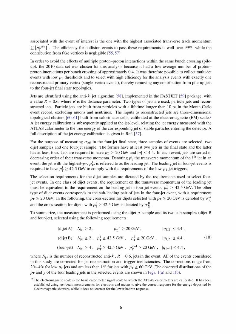
where Njet is the number of reconstructed anti-kt, R = 0.6, jets in the event. All of the events consideredin this study are corrected for jet reconstruction and trigger inefficiencies. The corrections range from2%–4% for low pT jets and are less than 1% for jets with pT ≥ 60 GeV. The observed distributions of thepT and y of the four leading jets in the selected events are shown in Figs. 1(a) and 1(b).2 The electromagnetic scale is the basic calorimeter signal scale to which the ATLAS calorimeters are calibrated. It has been

established using test-beam measurements for electrons and muons to give the correct response for the energy deposited byelectromagnetic showers, while it does not correct for the lower hadron response.

6

[GeV]T

p

100 200 300 400

Ent

ries/

10 [G

eV]

-110

1

10

210

310

410

510

610

710

PreliminaryATLAS-1 = 7 TeV, 37 pbs

1T

Data p 2T

Data p3

TData p 4

TData p

= 0.6R jets, tkAnti-

42.5 GeV≥ 1T

p

20 GeV≥ 2,3,4

Tp

4.4≤| 1-4

η|

(a)

y

-4 -2 0 2 4

Ent

ries/

0.5

0

100

200

300

400

310×

PreliminaryATLAS-1 = 7 TeV, 37 pbs

1Data y

2Data y

3Data y

4Data y

= 0.6R jets, tkAnti-

42.5 GeV≥ 1T

p

20 GeV≥ 2,3,4

Tp

4.4≤| 1-4

η|

(b)

Figure 1: Distributions of the (a) transverse momentum, pT, and (b) rapidity, y, of the four highest-pT jets, denotedas p1−4

T and y1−4 in the figures, in four-jet events in data, selected in the phase-space defined in the figure.

4.2 Correction for detector effects

The correction for detector effects for each class of events is individually estimated using the Pythia6 MCsample. The same restrictions on the phase-space of reconstructed jets, defined in Eq. (10), are appliedon particle jets. The correction is given by

CA,Bnj =

NA,B reconj

NA,B particlenj

, (11)

where NA,B reconj (NA,B particle

nj ) is the number of n-jet events passing the (A or B) selection requirementsusing reconstructed (particle) jets.

The correction is sensitive to the migration of events into and out of the phase-space of the measurement.Due to the very steep jet pT spectrum in dijet and four-jet events, it is crucial to have a good agreementbetween the jet pT spectra in data and MC close to the selection threshold before calculating the correc-tion. Therefore, the jet pT threshold was lowered to 10 GeV and the fiducial |η | range was increased to4.5, and the events in the MC are re-weighted such that the jet pT-y distributions in data are reproducedby the MC. The value of α4j

2j (see Eq. (8)), as determined from the re-weighted MC, is

α4j2j = 0.94 ± 0.01 (stat.) ± 0.02 (syst.) , (12)

where the first uncertainty is statistical and the second uncertainty is systematic. The systematic uncer-tainty arising from model-dependence is determined from a comparison with an alternate re-weightingmethod and from deriving α4j

2j using Sherpa. Other systematic uncertainties are discussed in Section 6.

7

5 Determination of the fraction of DPS events

The main challenge in the measurement of σeff is to estimate the DPS contribution to the four-jet datasample. It is impossible to extract complete-DPS and semi-DPS candidate events on an event by eventbasis. Therefore, the usual approach is to fit the distributions of variables sensitive to cDPS and sDPS inthe data to a combination of expected templates for the SPS, cDPS and sDPS contributions. The templatesfor SPS and sDPS contributions are extracted from the AHJ MC sample, while the cDPS template isobtained by overlaying two dijet events from the data. The analysis assumes that the SPS and sDPStemplates from AHJ render properly the expected topologies, and no further attempt is made to quantifypossible theoretical uncertainties associated with this assumption. For the SPS template, this assumptionis supported by the good agreement observed between various distributions in the SPS samples in AHJand in Sherpa. To exploit the full spectrum of variables sensitive to the various contributions and theircorrelations, an artificial neural network (NN) is used for the classification [62].

5.1 Template samples

In events generated in AHJ, the outgoing partons can be assigned to the primary interaction from theAlpgen ME generator or to a secondary interaction, generated by Jimmy, based on the event record. Theformer are referred to as primary-scatter partons and the latter are referred to as secondary-scatter partons.The pT of secondary-scatter partons is required to be

ppartonT ≥ 15 GeV , (13)

in order to match the minimum pT of primary-scatter partons which is set by the matching scale betweenradiation generated as part of the ME and radiation generated as part of the parton shower in AHJ. Oncethe outgoing partons are classified, the jets in the event are matched to outgoing partons and the event isclassified as a SPS, cDPS or sDPS event.

The matching of jets to partons is done in the φ− y plane by calculating the angular distance between thejet and the outgoing parton as

∆Rparton−jet =

√(yparton − yjet)2 + (φparton − φjet)2 . (14)

For 99% of the primary-scatter partons, the parton is within the distance ∆Rparton−jet ≤ 1.0, which istherefore used as a requirement for the matching of jets and partons.

Events in which none of the leading four jets are matched to a secondary-scatter parton are selected forthe SPS sample. All of the soft MPI and underlying activity is therefore retained in the selected SPSevents.

In the simple picture of double parton scattering adopted here, the two dijet productions are largelyuncorrelated. Therefore, a four-jet cDPS event is constructed from two overlaid dijet events. To reduceany dependence of the measurement on the modelling of dijet production in MC, cDPS events are builtusing dijet events in the dijet A and dijet B samples selected from data (see Eq. (10)). However, in orderto avoid double counting with the sDPS final state, events in the dijet B sample with an additional jet withpT ≥ 20 GeV are rejected. Double counting would occur in case an event with three jets is overlaid witha dijet event, since such a final state is included in the sDPS sample.

8

The conditions which must be fulfilled in order for a given pair of events to be overlaid are the follow-ing:

• none of the four jets overlap, i.e., ∆R jet−jet > 0.6;

• the vertices of the two overlaid events are no more than 10 mm apart in the z direction;

The first condition ensures that none of the jets would have been merged if the four-jet event had beenreconstructed as a real event; the second condition avoids possible kinematic bias due to events wheretwo jet pairs originate from far-away vertices.

As will be discussed in Section 5.4, the topology of cDPS events constructed by overlaying two dijetevents is compared to the topology of cDPS events extracted from the AHJ sample. Events in AHJ areclassified as cDPS events if two of the four leading jets are matched to primary-scatter partons and theother two are matched to secondary-scatter partons.

Events in which three of the leading jets are matched to primary-scatter partons and the fourth jet ismatched to a secondary-scatter parton are classified as sDPS events. A sDPS sample cannot be con-structed by overlaying three-jet events and dijet events from data since it is impossible to know a-prioriwhether the three-jet event was the result of one or two partonic interactions.

5.2 Kinematic characteristics of event classes

In a DPS, two dijet productions occur and should result in pair-wise pT-balanced jets with a distance|φ1 − φ2 | ≈ π between the jets in each pair. In addition, the azimuthal angle between the two planes ofinteractions is expected to have a random distribution. In SPS, the pair-wise pT balancing of jets is not aslikely, therefore the topology of the four jets is expected to be different for DPS and SPS.

The topology of three of the jets in sDPS events would resemble the topology of the jets in SPS inter-actions. The jet initiated by the primary interaction is expected to be closer, in the φ − y plane, to theplane defined by that interaction. The jet produced in the secondary interaction would most likely not becorrelated with the other three jets in the event, neither in azimuth nor in rapidity.

In constructing possible differentiating variables, three guiding principles were followed:

1. use pair-wise relations that have the potential to differentiate SPS and cDPS topologies;

2. include angular relations between all jets in light of the expected topology of sDPS events;

3. attempt to construct variables least sensitive to systematic uncertainties.

The first two guidelines encapsulate the different characteristics of SPS and cDPS events. The thirdguideline led to the usage of ratios of pT in order to avoid large dependencies on the jet energy scale(JES) systematic uncertainties. Various studies, including the use of a principal component analysis [63],led to the following list of possible variables:

∆pTi j =

���~piT + ~p j

T���

piT + p jT

; ∆φi j =���φi − φ j

��� ; ∆yi j =���yi − y j

��� ;

|φ1+2 − φ3+4 | ; |φ1+3 − φ2+4 | ; |φ1+4 − φ2+3 | ;

(15)

9

where piT, ~p iT, yi and φi stand for the scalar and vectorial transverse momentum, rapidity and azimuthal

angle of jet i, respectively, with i = 1,2,3,4. The variables with the sub-script i j are calculated for allpossible combinations. The term φi+ j denotes the azimuthal angle of the four-vector obtained by the sumof jets i and j.

Normalized distributions in the SPS, cDPS and sDPS samples of the variables for which the three dis-tributions exhibit the largest differences are shown and discussed below. In the following, the pairingnotation {〈i, j〉〈k, l〉} is used to describe a cDPS event in which jets i and j originate from one interactionand jets k and l originate from the other. In 85% of cDPS events, the two leading jets originate from oneinteraction and jets 3 and 4 originate from the other.

Normalized distributions of the ∆pT12 and ∆pT

34 variables in the SPS, cDPS and sDPS samples are shownin Figs. 2(a) and (b). In the cDPS sample, the ∆pT

12 and ∆pT34 distributions peak at low values, indicating

that both the leading and the sub-leading jet pairs are balanced in pT. The small peak around unity is dueto events in which the correct pairing of the jets is {〈1,3〉〈2,4〉} or {〈1,4〉〈2,3〉}. In the SPS and sDPSsamples, the leading jet-pair exhibits a wider peak at higher values of ∆pT

12 compared to that in the cDPSsample. This indicates that the two leading jets are not well balanced in pT since a significant fraction ofthe hard-scatter momentum is carried by one (sDPS) or two (SPS) of the additional jets.

The balance between the dijet pairs seen in the ∆pT34 distribution in the cDPS sample is also seen in the

∆φ34 distribution, shown in Fig. 2(c). The distribution of ∆pT34 in both SPS and sDPS samples is driven

by the ∆φ34 distribution shown in Fig. 2(c). As expected, the ∆φ34 distribution is almost uniform for theSPS and sDPS samples. The correlation between the distributions of the ∆pT

34 and ∆φ34 variables can bereadily understood through the following approximation: p3

T ≈ p4T ≈ pT ≈ 20 GeV. The expression for

∆pT34 then becomes

∆pT34 =

���~p3T + ~p 4

T���

p3T + p4

T

≈

√2pT + 2pT cos (∆φ34)

2pT=

√1 + cos (∆φ34)√

2. (16)

The peak around unity observed in the ∆pT34 distributions in the SPS and sDPS samples is thus a direct

consequence of the Jacobian of the relation between ∆pT34 and ∆φ34.

The set of variables quantifying the distance between jets in rapidity, ∆yi j , is particularly important forthe sDPS topology. The color flow is different in SPS leading to the four-jet final state and results insmaller angles between the sub-leading jets. Hence, on average, smaller distances between non-leadingjets are expected in the SPS sample compared to the sDPS sample. This is observed in the comparison ofthe ∆y34 distributions shown in Fig. 2(d), where the distribution in the sDPS sample is wider than in theother two samples.

The study of the various distributions of the variables in the three samples is summed up as follows:

• strong correlations between all variables are observed - The ∆pTi j and ∆φi j variables are correlated

in a non-linear way, while geometrical constraints correlate the ∆yi j and ∆φi j variables. Transversemomentum conservation relates the φi+ j − φk+l variables with the ∆pT

i j and ∆φi j variables;

• a clear separation between all three samples is not observed in any of the variables - The variablesin which a large difference is observed between the SPS and cDPS distributions, e.g., ∆pT

34 , do notprovide any differentiating power between SPS and sDPS;

• all variables are important - In cDPS events, where the pairing of the jets is different from {〈1,2〉〈3,4〉},variables relating the other possible pairs, e.g., ∆φ13, may indicate which is the correct pairing.

These conclusions led to the decision to use a multivariate technique in the form of an NN.

10

12T

p∆

0 0.2 0.4 0.6 0.8 1

1/N

0.05

0.1

0.15

PreliminaryATLAS

= 7 TeVs

SPS - AHJ

cDPS - Data - overlay

sDPS - AHJ

= 0.6R jets, tkAnti-

42.5 GeV≥ 1T

p

20 GeV≥ 2,3,4

Tp

4.4≤| 1-4

η|

(a)

34T

p∆

0 0.2 0.4 0.6 0.8 1

1/N

0.05

0.1

0.15

PreliminaryATLAS

= 7 TeVs

SPS - AHJ

cDPS - Data - overlay

sDPS - AHJ

= 0.6R jets, tkAnti-

42.5 GeV≥ 1T

p

20 GeV≥ 2,3,4

Tp

4.4≤| 1-4

η|

(b)

34φ∆

0 1 2 3

1/N

0.05

0.1

0.15

PreliminaryATLAS

= 7 TeVs

SPS - AHJ

cDPS - Data - overlay

sDPS - AHJ

= 0.6R jets, tkAnti-

42.5 GeV≥ 1T

p

20 GeV≥ 2,3,4

Tp

4.4≤| 1-4

η|

(c)

34y∆

0 2 4 6 8

1/N

0.05

0.1

0.15

0.2

PreliminaryATLAS

= 7 TeVs

SPS - AHJ

cDPS - Data - overlay

sDPS - AHJ

= 0.6R jets, tkAnti-

42.5 GeV≥ 1T

p

20 GeV≥ 2,3,4

Tp

4.4≤| 1-4

η|

(d)

Figure 2: Normalized distributions of the variables, (a) ∆pT12 , (b) ∆pT

34 , (c) ∆φ34 and (d) ∆y34, defined in Eq. (15), forthe SPS, cDPS and sDPS samples as indicated in the legend. The shaded bands represent the statistical uncertaintiesfor each sample.

11

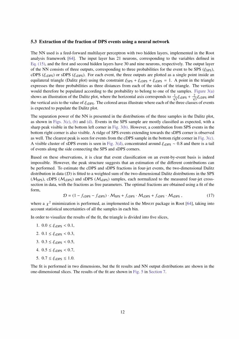
5.3 Extraction of the fraction of DPS events using a neural network

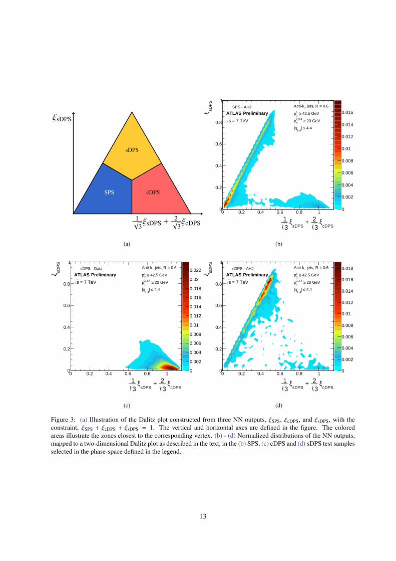
The NN used is a feed-forward multilayer perceptron with two hidden layers, implemented in the Rootanalysis framework [64]. The input layer has 21 neurons, corresponding to the variables defined inEq. (15), and the first and second hidden layers have 30 and nine neurons, respectively. The output layerof the NN consists of three outputs, corresponding to three probabilities for the event to be SPS (ξSPS),cDPS (ξcDPS) or sDPS (ξsDPS). For each event, the three outputs are plotted as a single point inside anequilateral triangle (Dalitz plot) using the constraint ξSPS + ξcDPS + ξsDPS = 1. A point in the triangleexpresses the three probabilities as three distances from each of the sides of the triangle. The verticeswould therefore be populated according to the probability to belong to one of the samples. Figure 3(a)shows an illustration of the Dalitz plot, where the horizontal axis corresponds to 1√

3ξsDPS + 2√

3ξcDPS and

the vertical axis to the value of ξsDPS. The colored areas illustrate where each of the three classes of eventsis expected to populate the Dalitz plot.

The separation power of the NN is presented in the distributions of the three samples in the Dalitz plot,as shown in Figs. 3(c), (b) and (d). Events in the SPS sample are mostly classified as expected, with asharp peak visible in the bottom left corner in Fig. 3(b). However, a contribution from SPS events in thebottom right corner is also visible. A ridge of SPS events extending towards the sDPS corner is observedas well. The clearest peak is seen for events from the cDPS sample in the bottom right corner in Fig. 3(c).A visible cluster of sDPS events is seen in Fig. 3(d), concentrated around ξsDPS ∼ 0.8 and there is a tailof events along the side connecting the SPS and sDPS corners.

Based on these observations, it is clear that event classification on an event-by-event basis is indeedimpossible. However, the peak structure suggests that an estimation of the different contributions canbe performed. To estimate the cDPS and sDPS fractions in four-jet events, the two-dimensional Dalitzdistribution in data (D) is fitted to a weighted sum of the two-dimensional Dalitz distributions in the SPS(MSPS), cDPS (McDPS) and sDPS (MsDPS) samples, each normalized to the measured four-jet cross-section in data, with the fractions as free parameters. The optimal fractions are obtained using a fit of theform,

D = (1 − fcDPS − fsDPS) · MSPS + fcDPS · McDPS + fsDPS · MsDPS , (17)

where a χ2 minimization is performed, as implemented in the Minuit package in Root [64], taking intoaccount statistical uncertainties of all the samples in each bin.

In order to visualize the results of the fit, the triangle is divided into five slices,

1. 0.0 ≤ ξsDPS < 0.1,

2. 0.1 ≤ ξsDPS < 0.3,

3. 0.3 ≤ ξsDPS < 0.5,

4. 0.5 ≤ ξsDPS < 0.7,

5. 0.7 ≤ ξsDPS ≤ 1.0.

The fit is performed in two dimensions, but the fit results and NN output distributions are shown in theone-dimensional slices. The results of the fit are shown in Fig. 5 in Section 7.

12

1√3ξsDPS + 2√

3ξcDPS

ξsDPS

SPS cDPS

sDPS

(a)

cDPSξ

32 +

sDPSξ

31

0 0.2 0.4 0.6 0.8 1sD

PS

ξ0

0.2

0.4

0.6

0.8

1

0

0.002

0.004

0.006

0.008

0.01

0.012

0.014

0.016 PreliminaryATLAS

= 7 TeVs

SPS - AHJ = 0.6R jets, tkAnti-

42.5 GeV≥ 1T

p

20 GeV≥ 2,3,4

Tp

4.4≤| 1-4

η|

(b)

cDPSξ

32 +

sDPSξ

31

0 0.2 0.4 0.6 0.8 1

sDP

Sξ

0

0.2

0.4

0.6

0.8

1

0

0.002

0.004

0.006

0.008

0.01

0.012

0.014

0.016

0.018

0.02

0.022 PreliminaryATLAS

= 7 TeVs

cDPS - Data = 0.6R jets, tkAnti-

42.5 GeV≥ 1T

p

20 GeV≥ 2,3,4

Tp

4.4≤| 1-4

η|

(c)

cDPSξ

32 +

sDPSξ

31

0 0.2 0.4 0.6 0.8 1

sDP

Sξ

0

0.2

0.4

0.6

0.8

1

0

0.002

0.004

0.006

0.008

0.01

0.012

0.014

0.016

0.018 PreliminaryATLAS

= 7 TeVs

sDPS - AHJ = 0.6R jets, tkAnti-

42.5 GeV≥ 1T

p

20 GeV≥ 2,3,4

Tp

4.4≤| 1-4

η|

(d)

Figure 3: (a) Illustration of the Dalitz plot constructed from three NN outputs, ξSPS, ξcDPS, and ξsDPS, with theconstraint, ξSPS + ξcDPS + ξsDPS = 1. The vertical and horizontal axes are defined in the figure. The coloredareas illustrate the zones closest to the corresponding vertex. (b) - (d) Normalized distributions of the NN outputs,mapped to a two-dimensional Dalitz plot as described in the text, in the (b) SPS, (c) cDPS and (d) sDPS test samplesselected in the phase-space defined in the legend.

13

5.4 Methodology validation

A sizable discrepancy was found in the ∆pT34 and ∆φ34 distributions between the data and AHJ (see Fig. 8

in the Appendix), suggesting that there are more sub-leading jets (jets 3 and 4) which are back-to-back inAHJ than in the data. In order to test that the discrepancies are not from mis-modelling of SPS in AHJ,the ∆pT

34 and ∆φ34 distributions in the SPS sample extracted from AHJ were compared to the distributionsin the SPS sample generated in Sherpa (see Fig. 9 in the Appendix). A good agreement in the shapesof the distributions was observed for both variables. This and further studies performed indicate that theexcess of events with jets 3 and 4 in the back-to-back topology is due to an excess of DPS events in theAHJ sample compared to the data.

In order to verify that the topology of cDPS events is reproducible by overlaying two dijet events, thedijet overlay sample is compared to the cDPS sample extracted from AHJ. An extensive comparisonbetween all the data and AHJ distributions used as inputs to the NN was performed and good agreementwas observed. This can be summarised by comparing the NN output distributions. The NN is applied tothe cDPS sample extracted from AHJ and the output distribution is compared to the output distributionof the cDPS sample constructed from dijets in data. Normalized distributions of the projection of thefull Dalitz plot on the horizontal axis are shown in Fig. 4, where a good agreement is observed betweenthe two distributions. Based on these results, it is concluded that the topology of the four jets in theoverlaid dijet events is comparable to that of the four leading jets in cDPS events extracted from AHJ. Anadditional advantage of using overlaid dijets from data to construct the cDPS sample is that the jets areat the same JES as the jets in four-jet events in data. This leads to a smaller systematic uncertainty in thefinal result.

As an additional validation step, the NN is applied to the inclusive AHJ sample and the resulting dis-tribution is fitted with the NN output distributions of the SPS, cDPS and sDPS samples (see Fig. 10 inthe Appendix). The fractions obtained from the fit, f (MC)

cDPS and f (MC)sDPS , are compared to the fractions at

parton-level, f (P)cDPS and f (P)

sDPS , extracted from the event record,

f (P)cDPS = 0.094 ± 0.001 (stat.), f (MC)

cDPS = 0.094 ± 0.003 (stat.),

f (P)sDPS = 0.048 ± 0.001 (stat.), f (MC)

sDPS = 0.041 ± 0.008 (stat.).(18)

The values obtained from the fit agree within their statistical uncertainties with those at parton-level. Thelarger statistical uncertainties on f (MC)

cDPS and f (MC)sDPS obtained by the fit reflect the loss of statistical power

due to the use of a template fit to estimate the fractions and the fact that their uncertainties are fullycorrelated.

6 Uncertainties

The combined statistical uncertainty on σeff is determined by performing many pseudo-experiments,∆σeff =+12.2

−9.4 %. The statistical uncertainty on α4j2j (of ∼1%) is propagated as a systematic uncertainty on

σeff . The systematic uncertainties associated with the integrated luminosity measurement (±3.5%), there-weighting of AHJ (±6%), the jet reconstruction efficiency (±0.1%) and the selection of single-vertexevents (±0.1%) are added in quadrature to the uncertainty on σeff . The combined uncertainty on σeff

due to the jet energy resolution uncertainty and the jet angular resolution uncertainties is ±12%. Various

14

cDPSξ

32 +

sDPSξ

31

0 0.2 0.4 0.6 0.8 1

1/N

0.02

0.04

0.06

0.08

0.1

0.12

PreliminaryATLAS

= 7 TeVs

cDPS - Data - overlaid dijets

cDPS - AHJ

= 0.6R jets, tkAnti-

42.5 GeV≥ 1T

p

20 GeV≥ 2,3,4

Tp

4.4≤| 1-4

η|

1.0≤ sDPS

ξ ≤0.0

Figure 4: Normalized distributions of the NN outputs, 1√3ξsDPS + 2√

3ξcDPS, in the range 0.0 ≤ ξsDPS ≤ 1.0 in cDPS

events extracted from AHJ (red dots), selected in the phase space defined in the figure, and in the cDPS sampleconstructed from dijet events in data (red histogram).

sources of uncertainty on the JES are considered [57] and their combined contribution amounts to +35−39%.

The relative systematic uncertainties on fDPS, α4j2j and σeff are summarized in Table 1. The dominant

systematic uncertainty on fDPS originates from the JES variation, mainly through large variations offsDPS. A variation in the JES results in modified NN output distributions in the sDPS and SPS templatesused in the fit to extract fcDPS and fsDPS. Due to the difficulty in differentiating between the sDPS andSPS topologies, and in particular the dependence on the transverse momentum of the fourth jet, the fsDPSvalue changes substantially when using distributions that are modified by the JES variation.

The stability of the measured value of σeff with respect to the various parameter values used in themeasurement was studied. Parameters such as pparton

T and ∆R jet−jet were varied and the requirement∆Rparton−jet ≤ 0.6 was applied, leading to a relative change in σeff of the order of a few percent. A fullstudy of the effects of these parameter values is not possible, as it would require repeating the measure-ment using a different set of observables, e.g., anti-kt jets with a distance parameter of 0.4 or generatinga new AHJ sample with a different matching scale. However, since the observed relative changes aresmall compared to the statistical uncertainty on σeff , no systematic uncertainty is assigned due to theseparameters.

15

Source of systematic uncertainty ∆ fDPS [%] ∆α4j2j [%] ∆σeff [%]

Luminosity ±3.5

Re-weighting of Pythia6 ±2 ±2

Re-weighting of AHJ ±6 ±6

Jet reconstruction efficiency ±0.1

Single-vertex events selection ±0.1

Jet energy and angular resolution ±16 ±5 ±12

JES uncertainty +64−43

+15−14

+35−39

Total systematic uncertainty +66−46

+16−15

+38−42

Table 1: Summary of the relative systematic uncertainties on fDPS , α4j2j and σeff .

7 Determination of σeff

To determine fDPS and σeff and their statistical uncertainties taking into account all of the correlations,many pseudo-experiments (fits) are performed. The systematic uncertainties are obtained by propagatingthe expected variations into the analysis and the resulting shifts are added in quadrature. The result forfDPS is

fDPS = 0.084 +0.009−0.012 (stat.) +0.054

−0.036 (syst.) , (19)

where the systematic uncertainties on fDPS are detailed in Table 1. The intermediate results for fcDPS andfsDPS can be quantified as

fcDPS = 0.052 +0.002−0.005 (stat.) ± 0.008 (syst.), fsDPS = 0.032 +0.008

−0.01 (stat.) +0.053−0.035 (syst.) , (20)

where the quoted systematic uncertainties do not include any positivity constraint on the fractions. Whentaking into account the systematic uncertainties of the templates in the calculation of the goodness-of-fitχ2 (without re-doing the fit), a value for χ2/NDF of 0.7 is obtained, where NDF is the number of degreesof freedom of the fit. This indicates that the sum of the SPS, cDPS and sDPS contributions after the fithas been performed provides a good description of the data.

A comparison of the fit distributions with the distributions in data in five one-dimensional slices of theDalitz plot is shown in Fig. 5. The statistical uncertainty in each bin in the fit distribution is shown asthe dark shaded area while the light shaded area represents their sum in quadrature with the systematicuncertainties. The distributions of the SPS, cDPS and sDPS contributions are also shown, normalized totheir respective fraction in the data as obtained by the fit. Considering the systematic uncertainties, themost significant disagreement with the data is seen for the left-most bin in the range 0.0 ≤ ξsDPS < 0.1(Fig. 5(a)) of the Dalitz plot. This bin is dominated by the SPS contribution. Thus, a discrepancy betweenthe data and the fit result in this bin is expected to have a negligible effect on the measurement of thedouble parton scattering rate.

The distributions of the ∆pT34 and ∆φ34 variables in data are compared to a combination of the distributions

in the three samples, SPS, cDPS and sDPS in Fig. 6. The latter three distributions are normalized to theirrespective fraction in the data as obtained by the fit. A good description of the data is achieved.

16

cDPSξ

32 +

sDPSξ

31

Ent

ries/

0.05

210

310

410

510

PreliminaryATLAS-1 = 7 TeV, 37 pbs

< 0.1sDPS

ξ ≤0.0

cDPSξ

32 +

sDPSξ

31

0 0.2 0.4 0.6 0.8 1

Dat

a/F

it

0.60.8

11.21.4

(a)

cDPSξ

32 +

sDPSξ

31

Ent

ries/

0.05

210

310

410

510

PreliminaryATLAS-1 = 7 TeV, 37 pbs

< 0.3sDPS

ξ ≤0.1

cDPSξ

32 +

sDPSξ

31

0.2 0.4 0.6 0.8 1

Dat

a/F

it

0.60.8

11.21.4

(b)

cDPSξ

32 +

sDPSξ

31

Ent

ries/

0.05

1

10

210

310

410

510

610 PreliminaryATLAS

-1 = 7 TeV, 37 pbs < 0.5

sDPSξ ≤0.3

cDPSξ

32 +

sDPSξ

31

0.2 0.4 0.6 0.8

Dat

a/F

it

0.60.8

11.21.4

(c)

cDPSξ

32 +

sDPSξ

31

Ent

ries/

0.05

1

10

210

310

410

510

PreliminaryATLAS-1 = 7 TeV, 37 pbs

< 0.7sDPS

ξ ≤0.5

cDPSξ

32 +

sDPSξ

31

0.3 0.4 0.5 0.6 0.7 0.8

Dat

a/F

it

0.60.8

11.21.4

(d)

cDPSξ

32 +

sDPSξ

31

Ent

ries/

0.02

1

10

210

310

410

510 PreliminaryATLAS

-1 = 7 TeV, 37 pbs 1.0≤

sDPSξ ≤0.7

cDPSξ

32 +

sDPSξ

31

0.5 0.6 0.7

Dat

a/F

it

0.60.8

11.21.4

(e)

Data 2010SPS - AHJcDPS - Data - overlaysDPS - AHJFit distribution (stat. uncertainty)Fit distribution (stat. + sys. uncertainty)

= 0.6R jets, tkAnti-

42.5 GeV≥ 1T

p

20 GeV≥ 2,3,4

Tp

4.4≤| 1-4

η|

Figure 5: Distributions of the NN outputs, 1√3ξsDPS + 2√

3ξcDPS, in the ξsDPS ranges indicated in the panels, for four-jet

events in data (dots), selected in the phase space defined in the legend, compared to the result of fitting a combinationof the SPS (blue histogram), cDPS (red histogram) and sDPS (yellow histogram) contributions, the sum of which isshown as the green histogram. In the fit distribution, statistical uncertainties are shown as the dark shaded area andthe light shaded area represents the sum in quadrature of the statistical and systematic uncertainties. The ratio of datato the fit distribution is shown in the bottom panels.

17

34T

p∆

Ent

ries/

0.05

410

510

PreliminaryATLAS-1 = 7 TeV, 37 pbs

34T

p∆

0 0.2 0.4 0.6 0.8 1

∑D

ata/

0.8

0.9

1

1.1

1.2

Data 2010SPS - AHJcDPS - Data - overlaysDPS - AHJ

of contributions∑(stat. uncertainty)

of contributions∑(stat. + sys. uncertainty)

= 0.6R jets, tkAnti-

42.5 GeV≥ 1T

p

20 GeV≥ 2,3,4

Tp

4.4≤| 1-4

η|

(a)

34φ∆

Ent

ries/

0.1

310

410

510

PreliminaryATLAS-1 = 7 TeV, 37 pbs

34φ∆

0 1 2 3

∑D

ata/

0.8

0.9

1

1.1

1.2

Data 2010SPS - AHJcDPS - Data - overlaysDPS - AHJ

of contributions∑(stat. uncertainty)

of contributions∑(stat. + sys. uncertainty)

= 0.6R jets, tkAnti-

42.5 GeV≥ 1T

p

20 GeV≥ 2,3,4

Tp

4.4≤| 1-4

η|

(b)

Figure 6: Comparison between the distributions of the variables (a) ∆pT34 and (b) ∆φ34, defined in Eq. (15), in four-

jet events in data (dots), selected in the phase space defined in the figure, and the sum (green histogram) of the SPS(blue histogram), cDPS (red histogram) and sDPS (yellow histogram) contributions. The sum of the contributionsis normalized to the cross-section measured in data and the various contributions are normalized to their respectivefractions obtained from the fit. In the sum of contributions distribution, statistical uncertainties are shown as the darkshaded area and the light shaded area represents the sum in quadrature of the statistical and systematic uncertainties.The ratio of data to the fit distribution is shown in the bottom panels.

18

Before calculating σeff , the symmetry factor in Eq. (9) has to be adjusted for the fact that there is anoverlap in the cross-sections σA

2j and σB2j when the leading jet in sample A has pT ≥ 42.5 GeV. The

adjusted symmetry factor is

11 + δAB

= 1 −12

σB2 j

σA2 j

= 0.9353 ± 0.0003 (stat.) , (21)

as determined from the measured cross-sections. It was also determined in Pythia6 and a good agreementwas observed between the two values. The relative difference in the value of σeff obtained by using thesymmetry factors extracted from the data and from Pythia6 is of the order of 0.2%, a negligible differencecompared to the statistical uncertainty on σeff .

An additional correction of about 4% is applied to the measured DPS cross-section due to the probabilityof jets from the secondary interaction to overlap with jets from the primary interaction. In such anoccurrence, the anti-kt algorithm would merge the two jets and the event would not be counted as a four-jet event. The value of the correction was determined from the fraction of phase-space occupied by a jet.It was also determined directly in AHJ and a good agreement between the two values was observed.

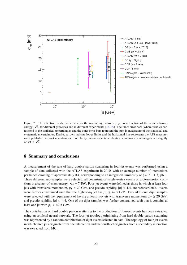
Once the fraction of double parton scattering in four-jet events in the data is estimated, and the symmetryfactor determined, the measurements of the dijet and four-jet cross-sections are used to calculate theeffective overlap area between the interacting protons, σeff , yielding

σeff = 16.1 +2.0−1.5 (stat.) +6.1

−6.8 (syst.) mb . (22)

This value is consistent within the quoted uncertainties with previous measurements, performed in AT-LAS and in other experiments [16–25], some of which are summarized in Fig. 7. Within the large un-certainties, the measurements are consistent with no

√s dependence of σeff . The σeff value obtained is

0.2 ± 0.1 of the measured value of σinel at√

s = 7 TeV as measured by ATLAS [65].

19

[GeV]s

210 310 410

[mb]

eff

σ

0

5

10

15

20

25

30

preliminaryATLAS ATLAS (4 jets)

- lower limit)ψATLAS (Z + J/

+ 3 jets, 2013)γD0 (

CMS (W + 2 jets)

ATLAS (W + 2 jets)

+ 3 jets)γDO (

+ 3 jets)γCDF (

CDF (4 jets)

UA2 (4 jets - lower limit)

AFS (4 jets - no uncertainties published)

Figure 7: The effective overlap area between the interacting hadrons, σeff , as a function of the center-of-massenergy,

√s, for different processes and in different experiments [16–25]. The inner error bars (where visible) cor-

respond to the statistical uncertainties and the outer error bars represent the sum in quadrature of the statistical andsystematic uncertainties. Dashed arrows indicate lower limits and the horizontal line represents the AFS measure-ment published without uncertainties. For clarity, measurements at identical center-of-mass energies are slightlyoffset in

√s.

8 Summary and conclusions

A measurement of the rate of hard double parton scattering in four-jet events was performed using asample of data collected with the ATLAS experiment in 2010, with an average number of interactionsper bunch crossing of approximately 0.4, corresponding to an integrated luminosity of (37.3 ± 1.3) pb−1.Three different sub-samples were selected, all consisting of single-vertex events of proton–proton colli-sions at a center-of-mass energy,

√s = 7 TeV. Four-jet events were defined as those in which at least four

jets with transverse momentum, pT ≥ 20 GeV, and pseudo-rapidity, |η | ≤ 4.4, are reconstructed. Eventswere further constrained such that the highest-pT jet has pT ≥ 42.5 GeV. Two additional dijet sampleswere selected with the requirement of having at least two jets with transverse momentum, pT ≥ 20 GeV,and pseudo-rapidity, |η | ≤ 4.4. One of the dijet samples was further constrained such that it contains atleast one jet with pT ≥ 42.5 GeV.

The contribution of hard double parton scattering to the production of four-jet events has been extractedusing an artificial neural network. The four-jet topology originating from hard double parton scatteringwas represented by a random combination of dijet events selected in data. The topology of four-jet eventsin which three jets originate from one interaction and the fourth jet originates from a secondary interactionwas extracted from MC.

20

The fraction of events that corresponds to the contribution made by hard double parton scattering infour-jet events was estimated to be,

fDPS = 0.084 +0.009−0.012 (stat.) +0.054

−0.036 (syst.) . (23)

Combining this with measurements of the dijet and four-jet cross-sections in the appropriate phase-spaceregions, the effective overlap area between the interacting protons, σeff , yields

σeff = 16.1 +2.0−1.5 (stat.) +6.1

−6.8 (syst.) mb .

This value is 0.2±0.1 of the measured value of σinel at√

s = 7 TeV. The σeff value obtained is consistentwith previous measurements performed at various center-of-mass energies and in various final states.This is compatible with a model in which σeff is a universal parameter that is process and phase-spaceindependent.

21

AppendixComparisons of the ∆pT

34 and ∆φ34 distributions in data and in AHJ are shown in Fig. 8. The distributionsin AHJ are rescaled to the cross-section measured in data. Also shown are the SPS, cDPS and sDPScontributions to the AHJ sample. A discrepancy between data and AHJ is observed in the region wherethe largest contribution of cDPS is expected.

34T

p∆

Ent

ries/

0.05

100

200

300

400

500

310×

PreliminaryATLAS-1 = 7 TeV, 37 pbs

Data 2010

AHJ

SPS - AHJ

cDPS - AHJ

sDPS - AHJ

= 0.6R jets, tkAnti-

42.5 GeV≥ 1T

p

20 GeV≥ 2,3,4

Tp

4.4≤| 1-4

η|

34T

p∆

0 0.2 0.4 0.6 0.8 1

Dat

a/A

HJ

0.8

0.91

1.1

1.2

(a)

34φ∆

Ent

ries/

0.1

50

100

150

200310×

PreliminaryATLAS-1 = 7 TeV, 37 pbs

Data 2010

AHJ

SPS - AHJ

cDPS - AHJ

sDPS - AHJ

= 0.6R jets, tkAnti-

42.5 GeV≥ 1T

p

20 GeV≥ 2,3,4

Tp

4.4≤| 1-4

η|

34φ∆

0 1 2 3

Dat

a/A

HJ

0.8

0.91

1.1

1.2

(b)

Figure 8: Comparison between the distributions of the variables (a) ∆pT34 and (b) ∆φ34, defined in Eq. (15), for four-

jet events in data and in Alpgen + Herwig + Jimmy (AHJ). Also shown are the SPS, cDPS and sDPS contributionsto the AHJ sample. The AHJ distributions are rescaled to the cross-section measured in data. The ratio of the datato AHJ is shown in the bottom panels, where the shaded bands represent the statistical uncertainties.

22

The distributions of the ∆pT34 and ∆φ34 variables are compared between the SPS sample extracted from

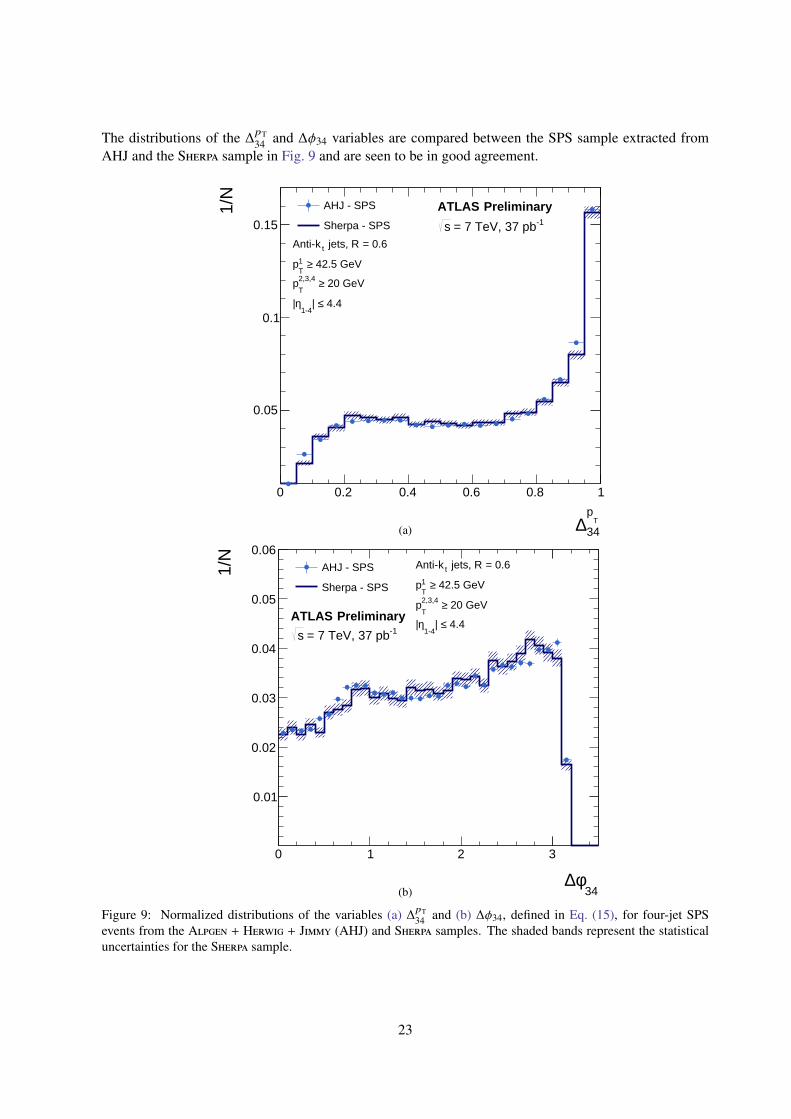
AHJ and the Sherpa sample in Fig. 9 and are seen to be in good agreement.

34T

p∆

0 0.2 0.4 0.6 0.8 1

1/N

0.05

0.1

0.15

PreliminaryATLAS-1 = 7 TeV, 37 pbs

AHJ - SPS

Sherpa - SPS

= 0.6R jets, tkAnti-

42.5 GeV≥ 1T

p

20 GeV≥ 2,3,4

Tp

4.4≤| 1-4

η|

(a)

34φ∆

0 1 2 3

1/N

0.01

0.02

0.03

0.04

0.05

0.06

PreliminaryATLAS-1 = 7 TeV, 37 pbs

AHJ - SPS

Sherpa - SPS

= 0.6R jets, tkAnti-

42.5 GeV≥ 1T

p

20 GeV≥ 2,3,4

Tp

4.4≤| 1-4

η|

(b)

Figure 9: Normalized distributions of the variables (a) ∆pT34 and (b) ∆φ34, defined in Eq. (15), for four-jet SPS

events from the Alpgen + Herwig + Jimmy (AHJ) and Sherpa samples. The shaded bands represent the statisticaluncertainties for the Sherpa sample.

23

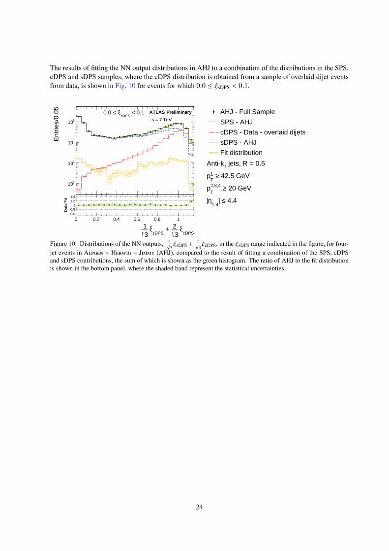
The results of fitting the NN output distributions in AHJ to a combination of the distributions in the SPS,cDPS and sDPS samples, where the cDPS distribution is obtained from a sample of overlaid dijet eventsfrom data, is shown in Fig. 10 for events for which 0.0 ≤ ξsDPS < 0.1.

cDPSξ

32 +

sDPSξ

31

Ent

ries/

0.05

210

310

410

510

PreliminaryATLAS

= 7 TeVs

< 0.1sDPS

ξ ≤0.0

cDPSξ

32 +

sDPSξ

31

0 0.2 0.4 0.6 0.8 1

Dat

a/F

it

0.60.8

11.21.4

AHJ - Full Sample

SPS - AHJ

cDPS - Data - overlaid dijets

sDPS - AHJ

Fit distribution

= 0.6R jets, tkAnti-

42.5 GeV≥ 1T

p

20 GeV≥ 2,3,4

Tp

4.4≤| 1-4

η|

Figure 10: Distributions of the NN outputs, 1√3ξsDPS + 2√

3ξcDPS, in the ξsDPS range indicated in the figure, for four-

jet events in Alpgen + Herwig + Jimmy (AHJ), compared to the result of fitting a combination of the SPS, cDPSand sDPS contributions, the sum of which is shown as the green histogram. The ratio of AHJ to the fit distributionis shown in the bottom panel, where the shaded band represent the statistical uncertainties.

24

References

[1] P. V. Landshoff and J. C. Polkinghorne, Calorimeter triggers for hard collisions, Phys. Rev. D18(1978) 3344.

[2] F. Takagi, Multiple Production of Quark Jets off Nuclei, Phys. Rev. Lett.43 (1979) 1296.

[3] C. Goebel, D. M. Scott, and F. Halzen, Double Drell-Yan annihilations in hadron collisions: Noveltests of the constituent picture, Phys. Rev. D22 (1980) 2789.

[4] R. Kirschner, Generalized Lipatov-Altarelli-Parisi equations and jet calculus rules, Phys. Lett. B84(1979) 266.

[5] V. P. Shelest, A. M. Snigirev, and G. M. Zinovev, The Multiparton Distribution Equations in QCD,Phys. Lett. B113 (1982) 325.

[6] M. Mekhfi, Correlations in Color and Spin in Multiparton Processes, Phys. Rev. D32 (1985) 2380.

[7] N. Paver and D. Treleani, Multi - Quark Scattering and Large pT Jet Production in HadronicCollisions, Nuovo Cim. A 70 (1982) 215.

[8] N. Paver and D. Treleani, Multiple Parton Interactions and Multi - Jet Events at Collider andTevatron Energies, Phys. Lett. B146 (1984) 252.

[9] M. Mekhfi, Multiparton Processes: An Application To Double Drell-yan, Phys. Rev. D32 (1985)2371.

[10] B. Humpert, Are There Multi - Quark Interactions?, Phys. Lett. B131 (1983) 461.

[11] B. Humpert, The production of gauge boson pairs by p anti-p colliders, Phys. Lett. B135 (1984)179.

[12] B. Humpert and R. Odorico, Multiparton scattering and QCD radiation as sources of four jetevents, Phys. Lett. B154 (1985) 211.

[13] L. Ametller, N. Paver, and D. Treleani, Possible signature of multiple parton interactions incollider four jet events, Phys. Lett. B169 (1986) 289.

[14] F. Halzen, P. Hoyer, and W. J. Stirling, Evidence for Multiple Parton Interactions From theObservation of Multi - Muon Events in Drell-Yan Experiments, Phys. Lett. B188 (1987) 375.

[15] R. M. Godbole, S. Gupta, and J. Lindfors, Double Parton Scattering Contribution To W + Jets, Z.Phys. C 47 (1990) 69.

[16] T. Akesson et al., Double parton scattering in pp collisions at√

s = 63 GeV, Z. Phys. C 34 (1986)163.

[17] J. Alitti et al., A study of multi-jet events at the CERN pp collider and a search for double partonscattering, Phys. Lett. B268 (1991) 145.

[18] CDF Collaboration, F. Abe et al., Study of four-jet events and evidence for double partoninteractions in pp collisions at

√s = 1.8 TeV, Phys. Rev. D47 (1993) 4857.

[19] CDF Collaboration, F. Abe et al., Measurement of double parton scattering in p̄p collisions at√

s = 1.8 TeV, Phys. Rev. Lett.79 (1997) 584.

25

[20] CDF Collaboration, F. Abe et al., Double parton scattering in pp collisions at√

s = 1.8TeV, Phys.Rev. D56 (1997) 3811.

[21] D0 Collaboration, V. Abazov et al., Double parton interactions in photon+3 jet events in p p-barcollisions

√s = 1.96 TeV, Phys. Rev. D81 (2010) 052012, arXiv:0912.5104 [hep-ex].

[22] D0 Collaboration, V. M. Abazov et al., Double parton interactions in photon + 3 jet and photon +

b/c jet + 2 jet events in ppbar collisions at sqrts=1.96 TeV, Phys. Rev. D89 (2014) 072006,arXiv:1402.1550 [hep-ex].

[23] ATLAS Collaboration, Measurement of hard double-parton interactions in W (→ lν)+ 2 jet eventsat√

s=7 TeV with the ATLAS detector, New J. Phys 15 (2013) 033038, arXiv:1301.6872[hep-ex].

[24] CMS Collaboration, Study of double parton scattering using W + 2-jet events in proton-protoncollisions at

√s = 7 TeV, JHEP 1403 (2014) 032, arXiv:1312.5729 [hep-ex].

[25] ATLAS Collaboration, Observation and measurements of the production of prompt andnon-prompt J/ψ mesons in association with a Z boson in pp collisions at

√s = 8 TeV with the

ATLAS detector, Eur. Phys. J. C75 (2015) 229, arXiv:1412.6428 [hep-ex].

[26] B. Blok, Y. Dokshitzer, L. Frankfurt, and M. Strikman, The Four jet production at LHC andTevatron in QCD, Phys. Rev. D83 (2011) 071501, arXiv:1009.2714 [hep-ph].

[27] J. R. Gaunt and W. J. Stirling, Double Parton Scattering Singularity in One-Loop Integrals, JHEP06 (2011) 048, arXiv:1103.1888 [hep-ph].

[28] B. Blok, Y. Dokshitser, L. Frankfurt, and M. Strikman, pQCD physics of multiparton interactions,Eur. Phys. J. C72 (2012) 1963, arXiv:1106.5533 [hep-ph].

[29] M. Diehl, D. Ostermeier, and A. Schafer, Elements of a theory for multiparton interactions inQCD, JHEP 03 (2012) 089, arXiv:1111.0910 [hep-ph].

[30] T. Kasemets and M. Diehl, Angular correlations in the double Drell-Yan process, JHEP 01 (2013)121, arXiv:1210.5434 [hep-ph].

[31] B. Blok, Yu. Dokshitzer, L. Frankfurt, and M. Strikman, Perturbative QCD correlations inmulti-parton collisions, Eur. Phys. J. C74 (2014) 2926, arXiv:1306.3763 [hep-ph].

[32] M. Diehl, T. Kasemets, and S. Keane, Correlations in double parton distributions: effects ofevolution, JHEP 1405 (2014) 118, arXiv:1401.1233 [hep-ph].

[33] J. R. Gaunt, Glauber Gluons and Multiple Parton Interactions, JHEP 07 (2014) 110,arXiv:1405.2080 [hep-ph].

[34] J. R. Gaunt, R. Maciula, and A. Szczurek, Conventional versus single-ladder-splittingcontributions to double parton scattering production of two quarkonia, two Higgs bosons andcc̄cc̄, Phys. Rev. D90 (2014) 054017, arXiv:1407.5821 [hep-ph].

[35] D. Treleani, Double parton scattering, diffraction and effective cross section, Phys. Rev. D76(2007) 076006, arXiv:0708.2603 [hep-ph].

[36] M. Bahr, M. Myska, M. H. Seymour, and A. Siodmok, Extracting σeffective from the CDFgamma+3jets measurement, JHEP 1303 (2013) 129, arXiv:1302.4325 [hep-ph].

26

[37] ATLAS Collaboration, The ATLAS Experiment at the CERN Large Hadron Collider, JINST 3(2008) S08003.

[38] ATLAS Collaboration, Performance of the ATLAS Trigger System in 2010, Eur. Phys. J. C72(2012) 1849, arXiv:1110.1530 [hep-ex].

[39] M. L. Mangano, M. Moretti, F. Piccinini, R. Pittau, and A. D. Polosa, ALPGEN, a generator forhard multiparton processes in hadronic collisions, JHEP 07 (2003) 001, arXiv:hep-ph/0206293.

[40] J. Pumplin et al., New generation of parton distributions with uncertainties from global QCDanalysis, JHEP 07 (2002) 012, arXiv:0201195 [hep-ph].

[41] J. Butterworth, J. R. Forshaw, and M. Seymour, Multiparton interactions in photoproduction atHERA, Z. Phys. C 72 (1996) 637, arXiv:hep-ph/9601371 [hep-ph].

[42] G. Corcella et al., HERWIG 6.5: an event generator for Hadron Emission Reactions WithInterfering Gluons (including supersymmetric processes), JHEP 01 (2001) 010,arXiv:hep-ph/0011363.

[43] ATLAS Collaboration, New ATLAS event generator tunes to 2010 data, Tech. Rep.ATL-PHYS-PUB-2011-008, CERN, 2011. https://cds.cern.ch/record/1345343.

[44] M. L. Mangano, M. Moretti, and R. Pittau, Multijet matrix elements and shower evolution inhadronic collisions: W bb̄ + n jets as a case study, Nucl. Phys. B 632 (2002) 343,arXiv:hep-ph/0108069 [hep-ph].

[45] F. Krauss, R. Kuhn, and G. Soff, AMEGIC++ 1.0: A Matrix element generator in C++, JHEP 02(2002) 044, arXiv:hep-ph/0109036 [hep-ph].

[46] T. Gleisberg, S. Hoeche, F. Krauss, M. Schonherr, S. Schumann, F. Siegert, and J. Winter, Eventgeneration with SHERPA 1.1, JHEP 0902 (2009) 007, arXiv:0811.4622 [hep-ph].

[47] H.-L. Lai, M. Guzzi, J. Huston, Z. Li, P. M. Nadolsky, J. Pumplin, and C. P. Yuan, New partondistributions for collider physics, Phys. Rev. D 82 (2010) 074024, arXiv:1007.2241 [hep-ph].

[48] S. Catani, F. Krauss, R. Kuhn, and B. Webber, QCD matrix elements + parton showers, JHEP 0111(2001) 063, arXiv:hep-ph/0109231 [hep-ph].

[49] F. Krauss, Matrix elements and parton showers in hadronic interactions, JHEP 0208 (2002) 015,arXiv:hep-ph/0205283 [hep-ph].

[50] T. Sjostrand, S. Mrenna, and P. Z. Skands, PYTHIA 6.4 Physics and Manual, JHEP 0605 (2006)026, arXiv:hep-ph/0603175 [hep-ph].

[51] A. Sherstnev and R. Thorne, Parton Distributions for LO Generators, Eur. Phys. J. C55 (2008)553, arXiv:0711.2473 [hep-ph].

[52] ATLAS Collaboration, Charged-particle multiplicities in pp interactions measured with the ATLASdetector at the LHC, New J. Phys 13 (2011) 053033, arXiv:1012.5104 [hep-ex].

[53] GEANT4 Collaboration, S. Agostinelli et al., GEANT4: A Simulation toolkit, Nucl. Instrum.Meth.A 506 (2003) 250.

[54] ATLAS Collaboration, The ATLAS Simulation Infrastructure, Eur. Phys. J. C70 (2010) 823,arXiv:1005.4568 [physics.ins-det].

27

[55] ATLAS Collaboration, Measurement of inclusive jet and dijet production in pp collisions at√

s = 7 TeV using the ATLAS detector, Phys. Rev. D86 (2012) 014022, arXiv:1112.6297[hep-ex].

[56] ATLAS Collaboration, Improved luminosity determination in pp collisions at sqrt(s) = 7 TeV usingthe ATLAS detector at the LHC, Eur. Phys. J. C73 (2013) 2518, arXiv:1302.4393 [hep-ex].

[57] ATLAS Collaboration, Jet energy measurement with the ATLAS detector in proton-protoncollisions at

√s = 7 TeV, Eur. Phys. J. C73 (2013) 2304, arXiv:1112.6426 [hep-ex].

[58] M. Cacciari, G. P. Salam, and G. Soyez, The Anti-k(t) jet clustering algorithm, JHEP 0804 (2008)063, arXiv:0802.1189 [hep-ph].

[59] M. Cacciari and G. P. Salam, Dispelling the N3 myth for the kt jet-finder, Phys. Lett. B 641 (2006)57, arXiv:hep-ph/0512210.

[60] C. Cojocaru et al., Hadronic calibration of the ATLAS liquid argon end-cap calorimeter in thepseudorapidity region 1.6 < |η | < 1.8 in beam tests, Nucl. Instrum. Meth.A 531 (2004) 481.

[61] W. Lampl et al., Calorimeter clustering algorithms: description and performance, Tech. Rep.ATL-LARG-PUB-2008-002, April, 2008. https://cds.cern.ch/record/1099735.

[62] D. Michie, D. J. Spiegelhalter, and C. C. Taylor, Machine Learning, Neural and StatisticalClassification. Ellis Horwood, New York, NY, 1994.

[63] I. T. Jolliffe, Principal Component Analysis. Springer Series in Statistics. Springer-Verlag, 2 ed.,2002.

[64] R. Brun and F. Rademakers, ROOT: An object oriented data analysis framework, Nucl. Instrum.Meth.A389 (1997) 81.

[65] ATLAS Collaboration, Measurement of the total cross section from elastic scattering in ppcollisions at

√s = 7 TeV with the ATLAS detector, Nucl. Phys. B 889 (2014) 486,

arXiv:1408.5778 [hep-ex].

28