hands-on introduction to protein visualization · 2019-09-18 · hands-on introduction to protein...

The Ohio State UniversityDepartment of Chemistryand Biochemistry

Hands-on Introduction to

Protein Visualization

VMD Developer: John StoneRaul Araya-Secchi

Michelle Gray

Marcos Sotomayor

October 2014

This tutorial is based on a VMD tutorial version created by Jordi Cohen, Elizabeth

Villa, Marcos Sotomayor, and Klaus Schulten at the Theoretical and Computational

Biophysics Group (UIUC), which is available at

http://www.ks.uiuc.edu/Training/Tutorials/

CONTENTS 2

Contents

1 Basics of Protein Visualization in VMD 51.1 Loading Molecules . . . . . . . . . . . . . . . . . . . . . . . . . . 51.2 Displaying Molecules . . . . . . . . . . . . . . . . . . . . . . . . . 61.3 Exploring Different Drawing Styles . . . . . . . . . . . . . . . . . 71.4 Exploring Different Coloring Methods . . . . . . . . . . . . . . . 101.5 Exploring Different Selections . . . . . . . . . . . . . . . . . . . . 101.6 Multiple Representations . . . . . . . . . . . . . . . . . . . . . . . 121.7 Sequence Viewer Extension . . . . . . . . . . . . . . . . . . . . . 131.8 Saving your Work . . . . . . . . . . . . . . . . . . . . . . . . . . 15

2 Multiple Molecules and Spatial Superposition 182.1 Loading Multiple Molecules . . . . . . . . . . . . . . . . . . . . . 182.2 Using the VMD Main Window . . . . . . . . . . . . . . . . . . . 192.3 Drawing representations for different molecules . . . . . . . . . . 202.4 Superposing molecules in space . . . . . . . . . . . . . . . . . . . 22

3 Trajectories and Scripting 263.1 Loading Trajectories . . . . . . . . . . . . . . . . . . . . . . . . . 263.2 VMD Main Window Animation Tools . . . . . . . . . . . . . . . 283.3 Labels . . . . . . . . . . . . . . . . . . . . . . . . . . . . . . . . . 303.4 Tcl Scripting Basics and the Tk Console . . . . . . . . . . . . . . 333.5 The atomselect Command . . . . . . . . . . . . . . . . . . . . . 353.6 An Example Tcl Script: Molecular Separation in a Trajectory . 38

CONTENTS 3

Introduction

This tutorial introduces biochemists to protein visualization and analysis ofmolecular dynamics trajectories using VMD. It is based on a version created atthe Theoretical and Computational Biophysics Group at the University of Illi-nois at Urbana-Champaign. The tutorial is designed specifically for VMD 1.9.1or later versions, and should take about 2 to 3 hours to complete in its entirety.Download and install VMD to start with tutorial instructions.

The examples in the tutorial will focus on the study of two tip link cadherinproteins that mediate hearing. Throughout the text, some material will be pre-sented in separate “boxes”. These boxes include complementary information tothe tutorial, such as information about the biological role of “tip links”, andtips or shortcuts for using VMD.

Tip links. This tutorial will focus on the visualization of the tip linkcadherins with VMD. Tip links are essential for hearing and bal-ance, and are made of two proteins interacting tip to tip: cadherin-23 (Cdh23) and protocadherin-15 (Pcdh15). These are large pro-teins with long extracellular domains formed by extracellular cad-herin (EC) repeats. The connection between Cdh23 and Pcdh15,the tip link bond, is mediated by the two most N-terminal EC re-peats of each protein. The primary function of the tip link is toconvey forces to the mechanosensitive channels that mediate oursenses of hearing and balance.

CONTENTS 4

Required programs

The following programs are required for this tutorial:

• VMD: Available at http://www.ks.uiuc.edu/Research/vmd/ (for all plat-forms)

• Plotting Program: The very last part of the tutorial requires you to plotoutput from VMD using an external application. Some examples include:

– Unix/Linux: xmgrace, http://plasma-gate.weizmann.ac.il/Grace/

– Windows: Excel, http://office.microsoft.com/en-us/FX010858001033.aspx(Purchase required)

– Mac/Multiple Platforms: Mathematica, http://www.wolfram.com/(Purchase required); gnuplot, http://www.gnuplot.info/(Free down-load)

Getting Started

You can find the files for this tutorial in the vmd-tutorial-files directory.Below you can see in Fig. 1 the files and directories of vmd-tutorial-files.

Figure 1: Directory structure of vmd-tutorial-files

To start VMD type vmd in a Unix terminal window, double-click on the VMDapplication icon in the Applications folder in Mac OS X, or click on the Start→ Programs → University of Illinois → VMD menu item in Windows.

1 BASICS OF PROTEIN VISUALIZATION IN VMD 5

1 Basics of Protein Visualization in VMD

In this unit you will build a nice image of the Cdh23 EC1 protein fragment whilegetting used to basic VMD commands. In addition, you will learn how to lookfor interesting structural properties of proteins using VMD.

1.1 Loading Molecules

Our first step is to load our moleculeof interest. A pdb file, 2WBX.pdb,that contains the atom coordinates ofthe Cdh23 EC1 protein fragment isprovided with the tutorial.

1 Choose the File→ New Molecule...menu item (Fig. 2a) in the VMDMain window. Another window,the Molecule File Browser (b), willappear in your screen.

2 Use the Browse... (c) but-ton to find the file 2WBX.pdb invmd-tutorial-files. Note thatwhen you select the file, youwill be back in the Molecule FileBrowser window. To actually loadthe file you have to press Load (d).Do not forget to do this!

Figure 2: Loading a Molecule.

Now, the Cdh23 protein fragment is shown in your screen in the OpenGL Dis-play window. You may close the Molecule File Browser window at any time.

Webpdb. VMD can download a pdb file from the Protein DataBank if a network connection is available. Just type the four lettercode of the protein in the File Name text entry of the Molecule FileBrowser window and press the Load button. For instance, you cantype 2WBX and VMD will download it automatically.

Coordinates file. The file 2WBX.pdb corresponds to the X-ray struc-ture of Cdh23 EC1 refined at 1.5 A resolution reported by MarcosSotomayor, Wilhelm A Weihofen, Rachelle Gaudet, and David P.Corey, Neuron (2010) 66, 85. Note that the protein is surroundedby 105 water molecules, and that hydrogen atoms are not included.


1.2 Displaying Molecules

To see the 3D structure of the Cdh23 EC1 protein we will use the mouse inmultiple modes.

1 In the OpenGL Display, press thefirst (left) mouse button down andmove the mouse. Explore whathappens. This is the rotationmode of the mouse and allows youto rotate molecules around an axisparallel to the screen (Fig. 3a).

Figure 3: Rotation modes.

2 If you press the second (right) button and repeat the previous step, therotation will be done around an axis perpendicular to your screen (b) (forMac users, the second button is equivalent to hitting the command keywhile pressing the mouse button).

3 In the VMD Main window, lookat the Mouse menu (Fig. 4).Here, you will be able to switchthe mouse mode from Rotation toTranslation or Scale modes.

4 The Translation mode will allowyou to move the molecule aroundthe screen while holding the first(left) button down. While intranslation mode, you can changethe clipping plane by holding themouse middle button down.

Figure 4: Mouse modes.

5 The Scale mode will allow you to zoom in or out by moving the mousehorizontally while holding the first (left) button down.

It should be noted that the previous actions performed with the mouse donot change the actual coordinates of the displayed atoms.

Mouse modes. Note that each mouse mode has its own charac-teristic cursor and its own shortcut key (r: Rotate, t: Translate, s:Scale) that could be used instead of the Mouse menu. Be sure tohave the OpenGL Display window active when using the shortcuts.Additional information can be found in the VMD user’s guide.


Another useful option is the Mouse → Center menu item. It allows you tospecify the point around which rotations are done.

6 Select the Center menu item and pick one atom at one of the ends of theprotein; The cursor should display a cross.

7 Now, press r, rotate your molecules with the mouse and see how theymove around the point you have selected.

8 Select the Display → Reset View menu item to return to the default view.

The Display menu in the VMD Main window allows you to set multiple optionscontrolling the way your molecules are displayed. Here you will switch depth-perception and rendering parameters.

9 Choose the Display → Perspective menu item.

Depth Perception. In perspective mode, things nearer the cameraappear larger. The displayed image will not preserve scale relation-ships or parallelism of lines, with objects very close to the cameraappearing distorted. The orthographic projection mode preservesscales and parallelism relationships, but greatly reduces depth per-ception.

Another way VMD can represent depth is through “depth-cueing”, which en-hances three-dimensional perception but decreases the brightness of the scene.

10 Use the Display → Depth Cueing menus item to disable or enable thisfeature.

Finally, visualization of your molecule can be enhanced by using the GLSLRender Mode.

11 Select the Display → Render Mode → GLSL menu item.

If your computer supports GLSL, you should notice an improvement on thequality of the image displayed in the OpenGL Display window, specially in sub-sequent steps with more complex representations.

1.3 Exploring Different Drawing Styles

VMD can display your molecules using a wide variety of drawing styles. Here,we will explore those that can help you identify different structures in the pro-tein fragment you loaded.


1 Choose the Graphics → Represen-tations... menu item. A win-dow called Graphical Representa-tions will appear and you will seethe current graphical representa-tion used to display your moleculeshaded (Fig. 5a).

2 In the Draw Style tab (b) we canchange the style (d) and color (c)of the representation. In this sec-tion we will focus on the drawingstyle (the default is Lines).

3 Each Drawing Method has its ownparameters. For instance, changethe Thickness of the lines by usingthe controls on the right bottompart (e) of the Graphical Repre-sentations window.

Figure 5: Graphical Representationswindow.

4 Now, choose VDW (van der Waals) from Drawing Method. Each atom isrepresented by a sphere. In this way you can see more easily the volumetricdistribution of the molecule.

5 To see the arrangements of atoms in the interior of our protein, use the newcontrols on the right bottom part of the window (e) to change the SphereScale to 0.5 and the Sphere Resolution to 13. Be aware that the higherthe resolution, the slower the display of your molecule will be. Changes inresolution will not be perceived if GLSL is active, but are important forimage and movie rendering.

6 Note that in Coloring Method → Name, each atom has its own color, i.e:O is red, N is blue, C is cyan and S is yellow.

7 Press the Default button. This allows you to return to the default prop-erties of the drawing method.


More representations. Other interesting representations are CPKand Licorice. In the first one, like in old chemistry ball & stickkits, each atom is represented by a sphere and each bond is repre-sented by a cylinder (radius and resolution of both the sphere andthe cylinder can be modified independently). The Licorice drawingmethod (widely used) also represents each atom as a sphere andeach bond as a cylinder, but the sphere radius cannot be modifiedindependently.

Figure 6: Licorice, Tube and NewCartoon representations of Cdh23 EC1.

The previous representations allow you to see the atomic details of Cdh23 EC1.However, more general structural properties can be seen by using more abstractdrawing methods.

8 Choose the Tube style under Drawing Method and observe the backboneof your protein fragment. Set the Radius at 0.8.

9 By looking at your protein in the Tube mode, can you distinguish howmany helices, β sheets and coils are present?

The last drawing method we will explore is NewCartoon. It gives a simplifiedrepresentation of a protein based on its secondary structure. Helices are drawnas coiled ribbons, β sheets as solid arrows and all other structures as a tube.This is probably the most popular drawing method to view the overall architec-ture of a protein.

10 Choose Drawing Method → NewCartoon.

You can now try to identify how many helices, β-sheets, and coils are presentin this protein (Fig. 6).


Structure of a Cadherin EC fragment. Cadherin proteins havecadherin extracellular (EC) repeats with a typical fold and similar,but not identical, sequences. EC fragments or repeats are labeledEC1, EC2, and so on from N- to C- termini. Cdh23 EC1 has oneshort piece of 310-helix (residues 12 to 15), two turns of α-helix(residues 50 to 55), and seven β strands (residues 7 to 9 and 18 to20 for strand A; 28 to 32 and 35 to 36 for strand B; 44 to 48 forstrand C; 56 to 58 for strand D; 64 to 67 for strand E; 78 to 86 forstrand F; and 91 to 100 for strand G). There are several reverse turnsthat link the strands together to form a Greek-key motif. VMD usesthe program STRIDE to compute the secondary structure accordingto an heuristic algorithm.

1.4 Exploring Different Coloring Methods

1 Now, let’s modify the colors of our representation. Choose Coloring Method→ResType (Fig. 5c). This allows you to distinguish non-polar residues(white), basic residues (blue), acidic residues (red) and polar residues(green).

2 Select Coloring Method → Secondary Structure and confirm that the New-Cartoon representation displays colors consistent with secondary structure(Fig. 7).

Figure 7: NewCartoon representation of Cdh23 EC1 colored by Residue Type(left) and Secondary Structure (right).

1.5 Exploring Different Selections

Let’s look at different independent (and interesting) parts of our Cdh23 EC1protein fragment.


1 In the Selected Atoms text entry (Fig. 5f) of the Graphical Representationswindow delete the word all, type sheet and press the Apply button orhit the Enter/Return key on your keyboard (do this every time you typesomething). VMD will show all β-strands forming sheets for cdh23 EC1.Note that β-strands A and B are split in two separate segments each.

2 In the Graphical Representations window choose the Selections tab (Fig. 8a).In section Singlewords (b) you will find a list of possible selections you cantype. For instance, try to display α helices instead of β-strands by typingthe appropriate word in the Selected Atoms text entry.

Combinations of boolean operators can also be used when writing a selection.

3 To see the molecule without he-lices and β strands, type the fol-lowing in Selected Atoms: (not

helix)and(not betasheet)

4 Now, change the current represen-tation’s Drawing Method to CPKstyle and the Coloring Method toResName in the Draw Style tab.

5 In the section Keyword (c) of theSelections tab (a) you can seeproperties that can be used toselect parts of a protein with theirpossible values. Look at possiblevalues of the Keyword resname(d). Display all the Aspartates,Glutamates, and calcium ionspresent in the proteins by typ-ing (resname ASP)or(resname

GLU)or(resname CA). Note thatyou can also type resname ASP

GLU CA. Figure 8: Graphical Representationswindow and the Selections tab.

Charged amino acids like Aspartate and Glutamate play an important role incalcium coordination and binding of Cdh23 to its Pcdh15 partner.

6 In the Selected Atoms text entry type water. Choose Coloring Method →Name. You should see the 105 water molecules (in fact only the oxygens)present in our system.


7 To see which water molecules are closer to the protein you can use thecommand within. Type water and within 2.6 of protein. This se-lects all the water molecules that are within a distance of 2.6 angstromsof the protein.

8 Finally, try typing the following selections in Selected Atoms:

Selection Actionprotein Shows the proteinresid 1 The first residue(resid 1 102) and (not water) The first and last residues(resid 50 to 55) and (protein) The α helix

All the previous options provide you with powerful tools to explore differentparts of your protein.

1.6 Multiple Representations

The button Create Rep (Fig. 9a) inthe Graphical Representations windowallows you to create multiple repre-sentations. Therefore, you can havea mixture of different selections withdifferent styles and colors, all displayedat the same time.

1 For the current representation, setthe Drawing Method to NewCar-toon and the Coloring Method toSecondary Structure.

2 In Selected Atoms type protein.

3 Press the Create Rep button (a).Now, using the menu items of theDraw Style tab and the SelectedAtoms text entry, modify the newrepresentation to get Licorice asthe Drawing Method, Name asthe Coloring Method, and resname

ASP GLU typed in as the currentselection.

Figure 9: Multiple Representations.


4 Repeating the previous procedure, create the following two new represen-tations:

Drawing Style Coloring Method SelectionCPK Name water

VDW ColorID 18 resname CA

5 Create a final representation by pressing again the Create Rep button.Select Drawing Method → Surf, the Coloring Method → Molecule and typeprotein in the Selected Atoms entry. For this last representation choosein the Material section (c) the Transparent menu item.

Note that with the mouse you can select the different representations you havecreated and modify each one independently. Also, you can switch each oneon/off by double-clicking on them or delete each one by using the Delete Repbutton (b).

Figure 10: Cdh23 EC1.

6 Turn off the second and last representations. At the end of this section,the Graphical Representations window should look like Fig. 9, and yourprotein should look like Fig. 10.

1.7 Sequence Viewer Extension

When dealing with a protein for the first time, it is very useful to find anddisplay different amino acids quickly. The sequence viewer extension allows youto pick and display one or more residues easily.


1 Choose the Extensions → Analy-sis→ Sequence Viewer menu item.A window (Fig. 11a) with a listof the amino acids (e) and theirproperties (b&c) will appear inyour screen.

2 With the mouse, click over differ-ent residues (e) in the list and seehow they are highlighted. In ad-dition, the highlighted residue willappear in your OpenGL Displaywindow in yellow and bond draw-ing method, so you can visualizeit easily. Use the right button ofthe mouse to unselect residues.

Figure 11: Sequence window.

3 Using the Zoom controls (f) you can display the entire list of residues inthe window. This is especially useful for larger proteins.

4 Using the shift key while pressing the mouse button allows you to pickmultiple residues at the same time. Look at residues 4, 5, 37, 39, 41, and87 (e).

5 Look at the Graphical Representations window, you should find a newrepresentation with the residues you have selected using the SequenceViewer Extension. As you already did before, you can modify, hide ordelete this representation.

Cadherins and Calcium. Cadherin proteins are involved in calcium-dependent molecular bonds. The calcium ion at the tip of Cdh23EC1 clamps the N-terminus of the protein fragment to favor inter-actions with Pcdh15. Calcium is coordinated by sides-chains andbackbone atoms of residues 4, 5, 37, 39, 41, and 87 in EC1 (theones that you selected using the Sequence Viewer Extension).

Information about residues is color-coded (d) in columns and obtained fromSTRIDE. The B-value column (b) shows the B-value field (temperature factor).The struct column shows secondary structure (d), where each letter means:


T TurnE Extended conformation (β sheets)B Isolated bridgeH Alpha helixG 3-10 helixI Pi helixC Coil

Table 1: Secondary Structure codes used by STRIDE.

1.8 Saving your Work

The image that you have created using VMD can be saved, along with allrepresentations you have created, as a VMD state. This VMD state containsall the information needed to start a new VMD session from it, without losingwhat you have done.

1 In the VMD Main window, choose the File→ Save Visualization State menuitem. Write an appropriate name (e.g., myfirststate.vmd) and save it.

The File → Load Visualization State menu item will allow you to load a previ-ously saved VMD state, just like the file you saved. Although the VMD stateallows you to work with the image and explore the properties of our proteinusing VMD, you usually need pictures that can be used in articles or other kindof documents. VMD can render the image you created and generate an imagefile that can be used in other applications, as it is shown in the following steps.

2 Using all that you have learned until now, find an appropriate view ofthe protein by scaling, rotating, and translating the molecule. Turn dif-ferent representations on and off and improve the resolution and differentproperties of the selections you have made. If you want an image of highquality, put special attention to the resolution of each representation.

3 Be aware of the new representations you created with the Sequence ViewerExtension and hide or delete them if necessary.

Troubleshooting. If the directory path where you wish to save yourrendered images contains spaces, it may be necessary, before youuse the File Render Controls, to navigate to the directory you wishto place your file using the Tk Console (select the Extensions →Tk Console menu item). Use quotes around the path, i.e., type cd

‘‘C:\ Documents and Settings’’.


4 Before rendering the image,change the background color bychoosing the Graphics → Colorsmenu item. There (Fig. 12),choose the Display category, theBackground name, and the 8 whitecolor. The background should bewhite now.

5 Choose the File→ Render... menuitem. A window called File Ren-der Controls will appear in yourscreen (Fig. 13).

Figure 12: Color Controls window.

6 You can render the image using different packages. Pick TachyonInternalin the Render the current scene using menu if you are using Unix or MacOS X, otherwise pick Tachyon.

7 Write the name of the filewhere the image will be savedin the Filename text entry, i.e.,picture.tga or picture.dat

(default is plot.tga or plot.dat

depending on platform).

8 Press the Start Rendering but-ton and the file with your im-age will be created. Note thatthis could take some time. Youshould end up with an image filenamed picture.tga (MacOS Xor Unix) or picture.dat.bmp (onWindows). Figure 13: File Render Controls win-

dow.

9 Close the application that opened the image file to continue using VMD(ignore this instruction in Windows).

10 In the VMD Main window, select the File→ Save Visualization State menuitem. Write an appropriate name (e.g., myfirststate2.vmd) and save it.This way you can reproduce your image later on if needed.


Now you are done with the first unit of the tutorial. We hope you have learnedthe basic commands of VMD. Also, you have generated at least two files. Thefirst one is a VMD state that allows you to restart a VMD session, and use ormodify all what you did in this unit. The second file is an image file of yourprotein that can be used in other image-viewing applications.

Advanced VMD features and tutorials. VMD is a powerful soft-ware with multiple tools that can help you generate sophisticatedimages and movies of your proteins. Here we have focused on thebasics. The “Using VMD” and the ”VMD Images and Movies” tu-torials (http://www.ks.uiuc.edu/Training/Tutorials/) describe moreadvanced options and procedures that can help you take full advan-tage of VMD’s capabilities.

2 MULTIPLE MOLECULES AND SPATIAL SUPERPOSITION 18

2 Multiple Molecules and Spatial Superposition

In this second unit you will learn to deal with multiple molecules simultane-ously within one VMD session. To do so, the structures of Cdh23 EC1 andCdh23EC1+2 will be loaded and superposed. You will also load and spatiallysuperpose the structure of Pcdh15 EC1+2.

Start with a new VMD session. If you have just completed unit 1,you should quit VMD and then launch it again.

2.1 Loading Multiple Molecules

First, you will load some of the molecules needed for this session.

1 Open the Molecule File Browser from the File → New Molecule. . . menuitem.

You need to load the X-ray crystal structure of Cdh23 EC1. You can do thisin the same way you did in unit 1:

2 Use the Browse... button tofind the file 2WBX.pdb invmd-tutorial-files. Notethat when you select the file, youwill be back in the Molecule FileBrowser window. In order toactually load the file you have topress Load. Do not forget to dothis!

Now, the Cdh23 EC1 fragment isshown in your screen in the OpenGLDisplay window.

Figure 14: Molecule File Browser win-dow with New Molecule option high-lighted.

The X-ray crystal structure of Cdh23 EC1+2 has been solved as well (pdb code2WHV). Proceed to load it.

3 In the Molecule File Browser window, select New Molecule (Fig. 14) fromthe menu at the top of the window (next to Load files for:). Type 2WHV

in the Filename: text entry and then press the Load button. If a con-nection to the internet is not available, browse for the file 2WHV.pdb invmd-tutorial-files, then click on the Load button. You have just loadeda separate molecule with the Cdh23 EC1+2 structure.


You should now see two unaligned molecules. One is the structure of Cdh23EC1, while the other one is the structure of Cdh23 EC1+2.

Number of EC repeats in cadherins. Members of the cadherin su-perfamily of proteins have at least 2 EC repeats. Classical cadherins,involved in calcium-dependent cell adhesion, sport an extracellulardomain with 5 EC repeats, while cadherin-23 has up to 28, andprotocadherin-15 up to 12 (confusing nomenclature, we know!).

2.2 Using the VMD Main Window

You will now give names to your molecules so that you can identify them later.

1 Double-click on the name of the first molecule in the VMD Main windowmolecule listing. The Rename Molecule dialog box should pop up. Typein Cdh23 EC1. Do the same thing for the second molecule, and call itCdh23 EC1+2.

At this point, your VMD Main window should look like Fig. 15. In front ofthe molecule name, there are four letters that you can use to manipulate yourmolecules.

Figure 15: VMD Main window with Cdh23 EC1 and Cdh23 EC1+2 loaded intotwo separate molecules.

F stands for “Fixed,” meaning that the molecule won’t move when you movethe scene around. When the F is black, the molecule is fixed; when it is red, themolecule is mobile.

2 Double-click on the F to the left of a molecule description in the Mainform. Then, try translating the scene with the mouse while one moleculeis fixed. Do it again with both molecules fixed.


3 When you are done, unfix both molecules and select the Display →Reset View menu item to correctly reposition the two molecules relativeto each other.

4 Next, double-click on the D of one molecule. The D stands for “Displayed”and when the D is red it means that the molecule is hidden. You cancontrol the visibility of all your molecules by double-clicking D.

5 When you are done, make sure that both the Cdh23 EC1 and the Cdh23

EC1+2 molecules are “Displayed” and that none of them are “Fixed”.

6 Finally, double-click under the T column to the left of the Cdh23 EC1

molecule. The letter T should now appear in front of it. This makes itthe unique “top” molecule. Making a molecule top makes it a target formultiple commands.

2.3 Drawing representations for different molecules

Before we continue and superpose these structures, take a look at your OpenGLDisplay window. You have two cadherin structures shown in the same defaultrepresentation. To tell them apart, you can assign to them different represen-tations and colors.

1 Open the Graphical Representations window by choosing the Graphics →Representations... menu item from the VMD Main window.

2 Make sure 0:Cdh23 EC1 is selected in the Selected Molecule pull-downmenu on the top part of the Graphical Representations window. SelectDrawing Method → NewCartoon and pick Coloring Method → ColorID → 1red for coloring.

3 Click on the Create Rep button to create a new representation. Deletethe word all in the Selected Atoms text entry of the Graphical Repre-sentations window and type resname CA. Hit the Enter/Return key onyour keyboard. Then select Drawing Method → VDW and pick ColoringMethod → ColorID → 18 yellow3 for coloring. You should be able to seeone calcium ion displayed as a green sphere at the tip of the protein.

4 Click on the Create Rep button again to create a third representationthat shows amino acids coordinating the calcium ion. Change the selec-tion text to same residue as within 3 of resname CA, select DrawingMethod → Licorice, and pick Coloring Method → Name.

One of the molecules has a particular set of representation and colors. Let’snow switch to the other one (Fig. 16).


5 In the Graphical Representationswindow, select 1:Cdh23 EC1+2 inthe Selected Molecule pull-downmenu on top. Select NewCartoonfor the Drawing Method, and Col-orID→ 0 blue for Coloring Method.

6 Click on the Create Rep but-ton to create a new represen-tation. Delete the word all

in the Selected Atoms text en-try of the Graphical Representa-tions window and type resname

CA. Hit the Enter/Return key onyour keyboard. Then select Draw-ing Method → VDW and pick Col-oring Method → ColorID → 18yellow3 for coloring. You shouldbe able to see four calcium iondisplayed as yellowish spheres inCdh23 EC1+2.

7 Click on the Create Rep but-ton again to create a thirdrepresentation that shows aminoacids coordinating the calciumions. Change the selectiontext to same residue as within

3 of resname CA, select DrawingMethod → Licorice, and pick Col-oring Method → Name. Figure 16: Graphical Representations

window with 1:Cdh23 EC1+2 selected.

Note that calcium-coordinating amino acids are located at the tip of the pro-tein, and also at the linker between repeats EC1 and EC2.


Now your OpenGL Display windowshould show Cdh23 EC1 colored in redand Cdh23 EC1+2 colored in blue,both with calcium ions shown as greenspheres and with calcium-coordinatingamino acids shown in licorice (Fig. 17).

Figure 17: Cdh23 EC1 and EC1+2.

2.4 Superposing molecules in space

The two molecules shown in the OpenGL Display window have the EC1 frag-ment, yet they are not superposed in space so it is difficult to appreciate theirsimilarities. We will use the RMSD Tool to superpose them in space.

Root Mean Squared Deviation RMSD. The Root Mean SquaredDeviation (RMSD) is defined as:

RMSD =

√∑Natoms

i=1(riA − riB)2

Natoms(1)

where Natoms is the number of atoms whose positions are beingcompared, and riA and riB are the positions of the correspondingatoms in molecules A and B, respectively. The RMSD can be usedto superpose two similar structures by minimizing its value whenapplying rigid-body translations and rotations.

1 In the Main window, open the RMSD Tool window from the Extensions→Analysis → RMSD calculator menu item (Fig. 18).

2 In the text entry, delete residue 5 to 85 and type resid 5 to 85 and

not altloc B C. Leave the Backbone only box checked.

This creates a selection containing backbone atoms of amino acids 5 to 85 inboth molecules, without including alternate conformations (altloc). This willensure that the number of atoms being compared between the two molecules isthe same, a requisite of the algorithm we use.

Alternate conformations. High resolution crystals structures oftenfeature alternate conformations for amino acid side chains. Coor-dinates for all versions of an amino acid chain may be present in asingle PDB file. VMD will show and use both, unless the altloc

keyword is used to select for alternate conformations, usually labeledA to C.


3 Click the Align button. You should be able to see in your OpenGL Dis-play window how the two molecules get superposed, with the two EC1fragments almost perfectly overlapping.

4 Zoom in to appreciate the differ-ences in the EC1 region.

Note that differences are most pro-nounced at the very N-terminal tips,which usually are fairly flexible and canadopt multiple conformations.

5 Click the RMSD button to ob-tain a quantitative measure of thedifferences between the two EC1structures.

Figure 18: RMSD Tool window.

The comparison between EC1 fragments from these two crystal structures re-vealed minuscule differences, as expected. However, spatial superposition canhelp compare proteins that have similar, but not identical folds and structures.We will now load Pcdh15 EC1+2, and compare it to Cdh23 EC1+2.

6 Open the Molecule File Browser from the File → New Molecule. . . menuitem.

7 Use the Browse... button to find the file 4APX-A.pdb in vmd-tutorial-files.Remember to press Load in the Molecule File Browser window.

You should now be able to see three molecules in your OpenGL Display window.

8 Double-click on the name of the third molecule in the Main windowmolecule listing. The Rename Molecule dialog box should pop up. Typein Pcdh15 EC1+2.

Pcdh15 EC1+2 is shown in the default Lines Drawing Method and spatiallyseparated from the other two molecules. To change its representation and su-perpose it to Cdh23 follow these steps:

9 Select the Extensions → Visualization → Clone Representations menu item.The Clone Representations window should pop-up. There, set the From


Molecule pull-down menu to 0 Cdh23 EC1 and the To Molecule: pull-downmenu to 2 Pcdh15 EC1+2. Click on the Clone button. Pcdh15 EC1+2should appear now in NewCartoon, with calcium ions in VDW and calcium-coordinating amino acids in Licorice.

10 In the Graphical Representationswindow, select 2:Cdh23 EC1+2 inthe Selected Molecule pull-downmenu on top, and click on thefirst representation to select it.Then change its color by selectingColorID → 11 purple for ColoringMethod. Figure 19: Clone Representations win-

dow.

You should be able to see Pcdh15 EC1+2 in purple, drawn with the same repre-sentations used for Cdh23 EC1 and Cdh23 EC1+2, but still spatially separated.

11 To superpose Pcdh15 EC1 to Cdh23 EC1, go to the RMSD Tool windowand click on the All in memory button. This will updated the list ofmolecules available for the RMSD Tool. All three molecules should belisted.

12 Check that the text entry still says resid 5 to 85 and not altloc B

C and click on the Align button. Pcdh15 should now be superposed to theCdh23 molecules (Fig. 20).

Figure 20: Cdh23 EC1 (red), Cdh23 EC1+2 (blue), and Pcdh15 EC1+2 (pur-ple). All three molecules superposed using part of EC1 (residues 5 to 85).


The superposition is not perfect, but it is good enough to reveal a common foldfor EC1 of both proteins. Note how the EC2 repeats are not aligned, as theangle between EC1 and EC2 repeats is different for Cdh23 and Pcdh15. Use allwhat you have learned about VMD to identify which parts of Cdh23 EC1 andPcdh15 EC1 are similar to each other and which ones are not.

Cdh23 and Pcdh15 Tips. Cdh23 and Pcdh15 are proteins with longextracellular domains implicated in sound perception and deafness,as well as in blindness and cancer. The N-terminal tips of theseproteins feature important structural features that are relevant fortheir function. For instance, both of them have long N-termini attheir EC1 repeat, and large protrusions midway throughout β-strandA. These features are important for their binding as you will see inthe next unit.

This ends the second unit of the tutorial. Now you should be able to han-dle multiple molecules in one session, use different representations and coloringmethods for each, and superpose them to compare their structures effectively.

3 TRAJECTORIES AND SCRIPTING 26

3 Trajectories and Scripting

In unit 3 you will learn how to load trajectories from molecular dynamics sim-ulations, place labels on atoms and bonds, and use a simple script to calculatethe separation between two molecules throughout a simulated trajectory.

3.1 Loading Trajectories

You will now learn to load the time evolving coordinates of a system, calledtrajectories. You will be able to see a movie of your system.

Trajectory files are normally binary files that contain several sets of coordinatesfor the system. Each set of coordinates corresponds to one frame in time. Anexample of a trajectory file is a DCD file. Trajectory files do not contain theconnectivity information of the system contained in the protein structure files(PSF). So we first need to load the structure file and then add the trajectorydata with the coordinates to this file.

1 Start a new VMD session.

2 Open the Molecule File Browser from the File → New Molecule ... menuitem. Browse for the file complex.psf in vmd-tutorial-files, then clickon the Load button. You have just created a new molecule with a structure(connectivity) but no coordinates (nothing will appear on the screen!).

Keep the Molecule File Browser window open. Notice that the menu at thetop of the window now says 0: complex.psf. This ensures that the next file thatyou load will be added to that molecule (molecule ID 0). You do not need tochange this menu to New Molecule, since you are merging data with the PSF file.

Coordinate files and structure files. To save space, simulationoutput files usually contain only the atom coordinates and do notstore unchanging information such as the atom types, atom charge,segment names and bonds. The latter information is stored in aseparate “structure” file (e.g., a PSF file). To visualize the resultsof a simulation, you need to merge both a structure and a coordinatefile into the same molecule.

3 In the Molecule File Browser window, click on the Browse button. Makesure that complex.psf is selected on the menu. Browse for pulling.dcdin vmd-tutorial-files, click OK, and click on the Load button again.You will be able to see the frames as they are loaded into the molecule.

After the trajectory finishes loading, you will be looking at its last frame. Wewill now create representations that will help you look at the system more easily.


4 In the VMD Main window, click to go back to frame 0. Then chooseGraphics→ Representations... menu item to open the Graphical Represen-tations window. In the Selected Atoms text entry window, type segname

P1. Then select Drawing Method → NewCartoon and Coloring Method →ColorID → 23.

5 In the Graphics → Representations menu item, click on the Create Repbutton.

6 In the Selected Atoms text entry window, erase the text and type segname

P2. Then select Drawing Method → NewCartoon and Coloring Method →ColorID → 11.

7 In the Graphics → Representations menu item, click on the Create Repbutton to create a third representation.

8 In the Selected Atoms text entry window, erase the text that appears thereand replace it with resname CAL.

9 In the Draw Style tab, choose a VDW representation for this selection andcolor it yellow (ColorID 17). You should now see all 7 calcium ions presentin the system.

Cdh23 and Pcdh15 “Handshake” Complex. The tips of Cdh23and Pcdh15 have been shown to interact through an extended“handshake” bond essential for tip link function. The structure,solved at 1.65 A resolution, was also used for molecular dynam-ics simulations testing the mechanical strength of the bond (Mar-cos Sotomayor, Wilhelm A Weihofen, Rachelle Gaudet, and DavidP. Corey, Nature 492 128, 2012). Tip links are constantly undersound-induced tension, and unbinding of the complex is likely re-lated to temporary deafness due to loud sound. The trajectory youjust loaded is a simulation that mimics physiological stretching whilehearing a very loud sound.

10 Create a representation with the selection betasheet and backbone, chooseDrawing Method → Hbonds, and color it red selecting Coloring Method →Color ID. In the options, set Distance Cutoff to 3.2, Angle Cutoff to 30and Line Thickness to 5.

In the OpenGL Display window you should be able to distinguish and appre-ciate the most important features of the handshake complex, including Cdh23EC1+2 (blue), Pcdh15 EC1+2 (purple), calcium ions (green), and β-sheet hy-drogen bonds (red). Your system should now look similar to the one in Fig. 21.

Cadherin Mechanics. The elastic properties of cadherins dependon calcium ions and hydrogen bonding between residues in the pro-tein’s β strands. Calcium rigidifies the chain of EC repeats, alsopreventing mechanical unfolding. Hydrogen bonds between β sheetbackbone atoms give stability and their formation and rupture undermechanical stress confers EC repeats with their elastic properties.


Figure 21: Cdh23 and Pcdh15 complex.

3.2 VMD Main Window Animation Tools

Now that you have nice representations, you will be able to observe what hap-pens during your trajectory. The Animation Tools help you do that. The VMDMain window includes all the Animation Tools you need for navigating throughyour trajectories. These tools are located at the bottom of the window (Fig. 22).

Figure 22: Animation Tools

1 In the VMD Main window, click on the button in the lower left (Fig. 22a).

2 Try using the button to jump to the end of the trajectory and go backto the beginning with the button. You can see the final and initial


states of the trajectory, which correspond to the fully bound and partiallyunbound states of the complex.

You can click on the slider and drag it back and forth to navigatethrough your trajectory. You can stop at anytime you want, or go at the speedyou need. This is helpful when you are looking at a trajectory and want to spotthe time when something interesting happens.

3 Using the slider, observe the behavior of calcium ions and the C-terminalβ-strand hydrogen bonds throughout the trajectory. Partial unfoldingoccurs while the proteins unbind.

Unbinding versus Unfolding. The simulation example loaded inVMD was performed at 10 to 100 times faster pulling speeds than aloud sound-induced mechanical stimuli. During the trajectory, youcan see partial unfolding of β-strands G in both Cdh23EC1+2 andPcdh15 EC1+2, while the complex unbinds. At even faster stretch-ing speeds, the complex unfolds without unbinding. At lower, closerto physiological pulling speeds, the simulations predict that the com-plex unbinds without any unfolding. Note that this simulation wasperformed with the complex in a water box, but coordinates for wa-ter molecules have not been included in the provided files to reducetheir size.

On the lower part of the Animation tools (Fig. 22), you will find all the toolsnecessary to play an animation without using the slider. This is done with thePlay buttons (b,c,g,h), that go forward and backward.

There are two ways to change the speed of your animation. You can adjustit using the Speed Slider (Fig. 22f). You can also adjust the step size. This isdone using the Step Window (e). If this step is set to 3, the animation will showevery 3rd frame, so it will make it faster.

4 Set the step to 5, and play the trajectory. Note that it plays faster, but italso looks less smooth than before. However, this can come handy if youare looking at long trajectories.


Looping styles. When playing animations, you can choose between3 looping styles in the Style menu (Fig. 22d). These are “Once”,“Loop” and “Rock”. A nice trick:

• Go to the beginning of the trajectory (frame 0).

• Set the step number to the total number of frames in yourtrajectory (300).

• Set the style to “Rock”.

• Set the speed to lowest.

• Play (h).

You can see now a comparison between the first and the last frameof your trajectory. This trick is better than clicking on the Start andEnd buttons.

You can also jump to a frame in your trajectory, by entering the frame numberin the window at the left of the Animation Tools.

NOTE: The Animation Tools you learned cycle through the frames of the Topmolecule, but apply to all Active molecules.

3.3 Labels

VMD allows you to place labels to get information on a particular selection.We will now make use of those labels for fun and profit. Labels are selected withthe mouse. In this example, we will cover labels that can be placed on atomsand bonds, although angle and dihedral labeling is also possible.

1 Choose the Mouse → Labels → Atoms menu item. The mouse is now setto “Display Label for Atom” mode. You can now click on any atom onyour molecule and a label will be placed next to this atom. Clicking againon it will erase the label.

We will now try the same for bonds.

2 Choose the Mouse→ Label→ Bonds menu item. This selects the “DisplayLabel for Bond” mode.

You will make a VDW Representation for the α carbon of each protein C-terminus, to be used for the bond label. In the pulling simulation, both arepulled in opposite directions at a constant velocity of 0.25 A/ps.

3 Create a VDW Representation with the selection (resid 208 and name

CA and segname P1) or (resid 237 and name CA and segname P2), andcolor it green (ColorID 7).


4 Now that you can see the C-terminal Cα atoms, and the mouse is inthe “Display Label for Bond” mode, click on both Cα atoms (one afterthe other). You should get a line connecting the two atoms. The num-ber appearing next to the line is the distance between the two atoms inangstroms (Fig. 23).

Note that the color of labels can be changed using the Color Controls windowavailable from the Graphics → Colors menu item (use the Labels category).

Figure 23: Bond selection of Cα terminal atoms in simulation. Both atoms se-lected display labels in green. The bond is shown in black (white in your screen),with the value of the distance between the atoms in A displayed (117.05).

The value of the distance corresponds to the current frame.

There are more things you can do withlabels using the Labels window.

5 Select the Graphics→ Labels menuitem. The Labels window shouldpop-up.

6 On the top left side of the win-dow (Fig. 24), there is a pull-downmenu where you can choose thetype of label (Atoms, Bonds, An-gles, Dihedrals). For now, keep itin Atoms. You can see the list ofatoms for which you made a label.

Figure 24: Label window.


7 Click on one of the atoms listed in the window. You can see all theinformation of the atom displayed. You can delete, hide, or show the labelby clicking on the corresponding buttons.

The information about the atom corresponds to the current frame, and is up-dated as the frame is changed.

8 Now, in the Label window, choose the label type Bonds, and select thebond you labeled. Note that the information given corresponds to onlythe first atom in the bond, but the number in the Value field correspondsto the length of the bond in angstroms.

9 Select the bond you labeled between atoms GLU208:CA and HSD237:CA.

10 Click on the Graph tab and then click on the Graph button. This will createthe plot of the distance between these two atoms over time (Fig. 25). Youcan also save this data to a file by clicking on the Save button, and thenuse an external plotting program to visualize the data.

Labels. The shortcut keys for labels are 1: Atoms and 2: Bonds.You can use these instead of the Mouse menu. Be sure the OpenGLDisplay window is active when using these shortcuts.

Figure 25: Plots of selected bonds over time created with the Graph button andVMD’s internal MultiPlot program.

We will now create another representation that will help us monitor the separa-tion of a salt bridge essential for the binding of Cdh23 EC1+2 to Pcdh15 EC1+2.

11 Click on the Graphics → Representations... menu item to open the Graph-ical Representations window. In the Selected Atoms text entry window,type (segname P1 and resid 78) or (segname P2 and resid 113).Then select Drawing Method → Licorice and Coloring Method → Name.You should be able to see the salt bridge formed by Arginine 113 andGlutamate 78.


12 To create a bond, choose the Mouse→ Label→ Bonds menu item (or click2 while the OpenGL Display window is active).

13 Click on the Arginine’s Cζ and Glutamate’s Cδ atoms (one after the other).You should get a line connecting the two atoms of the side chains of theseamino acids.

14 Select the Graphics → Labels menu item. The new bond should appearlisted in the Label window. Select the new bond GLU78:CD ARG113:CZ,and while holding the “shift” key down on your keyboard, select theGLU208:CA HSD237:CA bond as well. Graph them by clicking on the Graphtab and then clicking on the Graph button.

The MultiPlot window should appear with two curves (blue and red) showingthe length of the bonds throughout the loaded trajectory (Fig. 25). The timedependence of these bond lengths can help us distinguish unfolding from un-binding events.

Arginine 113 and Deafness. As you learned in previous parts of thistutorial, Cdh23 and Pcdh15 are essential for the vertebrate senses ofhearing and balance. Human genetics has revealed that individualscarrying the R113G mutation (arginine replaced by glycine) are deaf(Zubair M. Ahmed et al, Human Genetics 124 215, 2008). Thestructure of the Cdh23 and Pcdh15 complex suggests that replacingthe long, charged arginine side chain for a neutral glycine weakensthe interaction with its glutamate partner compromising the strengthof the complex.

3.4 Tcl Scripting Basics and the Tk Console

VMD provides powerful tools for analysis of trajectories obtained using molec-ular dynamics simulations. These tools are best used through “scripts” thatcontain sets of commands to be executed to complete a task. VMD includessupport for the Tcl/Tk scripting language. This section will attempt to providethe minimal amount of scripting knowledge that you will need to take full ad-vantage of VMD.

The Tcl/Tk scripting language. Tcl is a rich language with manyfeatures and commands, in addition to the typical conditional andlooping expressions. Tk is an extension to Tcl that permits thewriting of graphical user interfaces with windows and buttons. Moreinformation and docs about the Tcl/Tk language can be found athttp://www.tcl.tk/doc.

To execute Tcl commands, you will be using a convenient text console calledTk Console.


1 Select the Extensions → Tk Console menu item. A console window shouldappear with a prompt (Fig. 26). You can now start entering Tcl/Tkcommands in it.

Figure 26: The Tk Console window.

You will initially focus on the very basics of Tcl/Tk. Here are Tcl’s set andputs commands:

set variable value – sets the value of variableputs $variable – prints out the value of variable

2 Try the following commands:

set x 10

puts "the value of x is: $x"

set text "some text"

puts "the value of text is: $text."

As you can see, $variable refers to the value stored in variable.

Here is a command that performs mathematical operations:

expr expression – evaluates a mathematical expression

3 Try experimenting with the expr command:

expr 3 - 8

set x 10

expr - 3 * $x

One of the most important aspects of Tcl is that you can embed Tcl commandsinto others by using brackets. A bracketed expression will automatically be sub-stituted by the return value of the expression inside the brackets:


[expr.] – represents the result of the expression inside the brackets

4 Create some commands using brackets and test them. Here is an example:

set result [ expr -3 * $x ]

puts $result

3.5 The atomselect Command

You can edit atomic properties using VMD’s atomselect command. The fol-lowing examples will show you how. First, however, let’s display our proteincomplex using a suitable representation.

1 Open the Labels window by selecting the Graphics → Labels menu item.Hide all atom and bond labels.

2 Open the Graphical Representations window using the Graphics → Repre-sentations. . . menu item.

3 Delete all representations using the Delete Rep button.

4 Click on the Create Rep button and type in protein as the atom selection.Change its Coloring Method to Beta and its Drawing Method to VDW. Yourmolecule should now appear as a white assembly of spheres.

The PDB B-factor field. The “B” field of a PDB file typicallystores the “temperature factor” for a crystal structure and is readinto VMD’s “Beta” field. Since we are not currently interested inthis information, we can recycle this field to store our own numericalvalues. VMD has a “Beta” coloring method, which colors atomsaccording to their B-factors. By replacing the Beta values for variousatoms, you can control the color in which they are drawn. This isvery useful when you want to show a property of the system thatyou have computed, which is not supported out-of-the-box by VMD.

You will now learn a very important Tcl command in VMD:

atomselect molid selection – creates a new atom selection

The first argument to atomselect is the molecule ID (shown to the very left ofthe VMD Main window), the second argument is a textual atom selection likewhat you have been using to describe graphical representations in unit 1. Theselection returned by atomselect is itself a command which you will learn touse.


5 Type set p [atomselect top "protein"] in the Tk Console window.This creates a selection containing all the atoms in the molecule and as-signs it to the variable p. Instead of a molecule ID (which is a number),we have used the shortcut “top” to refer to the top molecule.

The result of atomselect is a function. Thus, $p is now a function that per-forms actions on the contents of the “protein” selection.

6 Type $p num. Passing num to an atom selection returns the number ofatoms in that selection. Check that this number matches the number ofatoms for that molecule (as read from the VMD Main window), exceptfor the 7 calcium ions.

7 Type $p set beta 0. This resets the “beta” field (which is displayed) tobe zero for all atoms.

Atom selections reference the atoms in the original molecule. When you changea property (e.g. beta value) of some atoms through a selection, that change isreflected in all the other selections that contain those atoms.

8 Now, type set sel [atomselect top "hydrophobic"]. This creates aselection containing all the hydrophobic residues.

9 Let’s tag all hydrophobic atoms by setting their beta values to 1. Youshould know how to do this now: $sel set beta 1. If the colors in theOpenGL Display do not get updated, click on the Apply button at thebottom of the Graphical Representations window.

Examples of atomic properties. You can get and set many atomicproperties using atom selections, including segment, residue andatom names, position (x, y and z), charge, mass, occupancy andradius, just to name a few.

10 You will now change a physical property of the atoms to further illustratethe distribution of hydrophobic residues. Type $p set radius 0.5 tomake all the atoms smaller and easier to see through, and then $sel set

radius 1.5 to make the hydrophobic residues larger. The radius fieldaffects the way that some representations (e.g., VDW, CPK) are drawn.

You have now created a visual state that clearly distinguishes which parts ofthe protein are hydrophobic and which are hydrophilic. If you have followed theinstructions correctly, your protein should resemble Fig. 27.


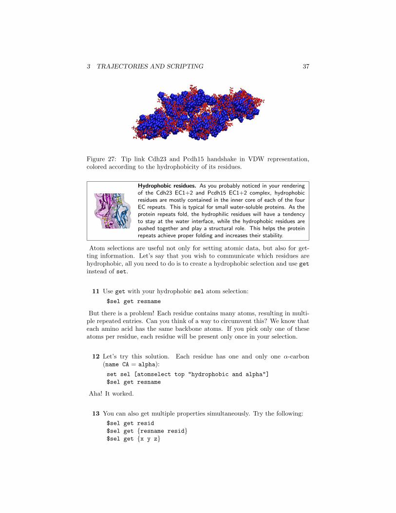
Figure 27: Tip link Cdh23 and Pcdh15 handshake in VDW representation,colored according to the hydrophobicity of its residues.

Hydrophobic residues. As you probably noticed in your renderingof the Cdh23 EC1+2 and Pcdh15 EC1+2 complex, hydrophobicresidues are mostly contained in the inner core of each of the fourEC repeats. This is typical for small water-soluble proteins. As theprotein repeats fold, the hydrophilic residues will have a tendencyto stay at the water interface, while the hydrophobic residues arepushed together and play a structural role. This helps the proteinrepeats achieve proper folding and increases their stability.

Atom selections are useful not only for setting atomic data, but also for get-ting information. Let’s say that you wish to communicate which residues arehydrophobic, all you need to do is to create a hydrophobic selection and use getinstead of set.

11 Use get with your hydrophobic sel atom selection:

$sel get resname

But there is a problem! Each residue contains many atoms, resulting in multi-ple repeated entries. Can you think of a way to circumvent this? We know thateach amino acid has the same backbone atoms. If you pick only one of theseatoms per residue, each residue will be present only once in your selection.

12 Let’s try this solution. Each residue has one and only one α-carbon(name CA = alpha):

set sel [atomselect top "hydrophobic and alpha"]

$sel get resname

Aha! It worked.

13 You can also get multiple properties simultaneously. Try the following:

$sel get resid

$sel get {resname resid}$sel get {x y z}


14 Once you are done with a selection, it is always convenient to delete themin order to save memory by typing:

$sel delete

3.6 An Example Tcl Script: Molecular Separation in aTrajectory

VMD is a powerful tool for MD analysis. In this section you will use Tclscripts to compute the distance between the center of mass of Cdh23 and Pcdh15throughout our unbinding trajectory.

1 The script we are going to use is called distance.tcl. This is the scriptcontent:

set outfile [open distance.dat w]

set nf [molinfo top get numframes]

set mol1 [atomselect top "segname P1"]

set mol2 [atomselect top "segname P2"]

# distance calculation loop

for { set i 1 } { $i <= $nf } { incr i } {$mol1 frame $i

$mol2 frame $i

set cmmol1 [measure center $mol1 weight mass]


set distance [veclength [vecsub $cmmol1 $cmmol2]]

puts $outfile "$i, $distance"

}close $outfile

2 The script does the following:

• Opens file distance.dat for writing

set outfile [open distance.dat w]

• Gets the number of frames in the trajectory and assign this value tothe variable nf

set nf [molinfo top get numframes]

• Makes a selection with atoms of Cdh23.

set all [atomselect top "segname P1"]

• Makes a selection with atoms of Pcdh15.

set all [atomselect top "segname P2"]


• Text after # denotes comment.

# distance calculation loop

• Loops over all frames in the trajectory:

for { set i 1 } { $i <= $nf } { incr i } {

• Changes the selection $mol1 to the frame being used for the calcula-tion (note that the content of the selection must be identical in everyframe, otherwise a $sel update command needs to be added).

$mol1 frame $i

• Changes the selection $mol2 to the current frame.

$mol2 frame $i

• Calculates the center of mass of the atoms stored in $mol1 and assignsit to cmmol1 as a vector.


• Calculates the center of mass of the atoms stored in $mol2 and assignsit to cmmol2 as a vector.


• Subtracts the vector stored in $cmmol2 from $cmmol1, then computesthe length of the vector resulting from the subtraction and assigns itto distance.

set distance [veclength [vecsub $cmmol1 $cmmol2]]

• Writes the calculated distance to file:

puts $outfile "$i, $distance"

Atom selections inside loops. The distance.tcl script describedabove does not create selections inside the distance calculation loop.However, if you need to create selections using the atomselect

command inside a loop, always remember to delete them using the$sel delete command. Otherwise you will run out of memory.

Now that you understand the script, you can use it for the system loaded inVMD to compute the distance between the center of mass of Cdh23 EC1+2 andPcdh15 EC1+2.


3 Type source distance.tcl in the Tk Console (be sure that your currentdirectory is vmd-tutorial-files). This will perform all the commandsin the script. The script will write a file distance.dat that will containthe value of the separation between the two molecules as a function offrame number.

Outside of VMD, you can use some plotting program to see this data. Exam-ples of these are gnuplot, xmgrace, excel, Mathematica (Fig. 28).

Figure 28: Plot of distance between the centers of mass of Cdh23 and Pcdh15as a function of frame number.

This ends our “Hands-on Introduction to Protein Visualization” tutorial. Wehope that you learned a lot with it, and that you will make great use of all the ca-pabilities VMD has to offer. Please visit http://www.ks.uiuc.edu/Training/Tutorials/and https://research.chemistry.ohio-state.edu/sotomayor/teaching/ for updatedversions of this and other tutorials.