handling concept drift based on data similarity and

UNIVERSIDADE FEDERAL DO AMAZONAS

INSTITUTO DE COMPUTAÇÃO - ICOMP

PROGRAMA DE PÓS-GRADUAÇÃO EM INFORMÁTICA – PPGI

Handling Concept Drift Based on Data

Similarity and Dynamic Classifier Selection

Felipe Azevedo Pinagé

Manaus - Amazonas July 2017







Tese apresentada ao Programa de Pós-

Graduação em Informática do Instituto

de Computação da Universidade Federal

do Amazonas como requisito parcial

para a obtenção do grau de Doutor em

Informática.

Orientadora: Eulanda Miranda dos

Santos

Manaus - Amazonas Julho de 2017







Thesis presented to the Graduate

Program in Informatics of the Institute of

Computing of the Federal University of

Amazonas in partial fulfillment of the

requirements for the degree of Doctor in

Informatics.

Advisor: Eulanda Miranda dos Santos

Manaus - Amazonas July 2017

iv

À minha família.

v

Acknowledgements

Primeiramente eu agradeço a Deus, pela força, pelas oportunidades e pelas pessoas que Ele pôs

no meu caminho ao longo desta jornada.

Aos meus pais, Elieuda e Mauro, meu muito obrigado por estarem ao meu lado em todos os

momentos, apoiando-me e proporcionando-me oportunidades que tornaram a minha caminhada

mais fácil. Quero agradecer também pelo amor, pelo carinho, e por sempre terem acreditado no

meu trabalho.

À minha irmã e ao meu cunhado, Monik e Ramon, por serem companheiros de muitas horas e

por permanecerem comigo, mesmo que por muitas vezes eu não faça por merecer. Meus

sinceros agradecimentos.

À minha orientadora, Professora Eulanda Miranda dos Santos, por todo apoio que tem me dado

desde o mestrado, pelas valiosas contribuições, conhecimento compartilhado e pela confiança

que sempre depositou em mim. Muito obrigado!

Ao meu supervisor durante minha estada na Universidade do Porto, Professor João Gama, por

ter me recebido de braços abertos, por toda a disposição para me auxiliar durante os estudos da

pesquisa e por todas as suas valiosas contribuições.

Aos professores, Alceu Brito Jr, Anne Canuto, Eduardo Souto e José Reginaldo por terem

aceitado participar da banca.

Às minhas avós, Eunice e Rosa, pelo amor incondicional.

Às minhas tias, Cláudia e Anne, por me amarem como um filho, e que assim como meus pais,

estão sempre ao meu lado me apoiando em tudo na minha vida. Meus eternos agradecimentos.

vi

À Elda Nunes, que esteve comigo desde a graduação, e por ser a amiga mais leal, que não só eu,

mas que qualquer pessoa pode ter. Muito obrigado por estar sempre ao meu lado.

Aos meus eternos amigos, Eduardo Sales, Érica Souza e Geangelo Calvi, por terem

compartilhado todos os momentos bons e me amparado em todos os momentos difíceis.

Aos amigos da Uninorte, Natacsha e Lucho, pela parceria e por tornarem minhas noites de

trabalho muito mais divertidas.

Aos amigos que fiz em Portugal, que por um ano de doutorado sanduíche fizeram com que eu

me sentisse em casa, dividindo essa fase única da minha vida.

Por fim, um agradecimento especial ao Programa de Pós-Graduação em Informática da UFAM

pela oportunidade proporcionada e à FAPEAM e CAPES, pelo apoio financeiro.

vii

Resumo

Em aplicações do mundo real, algoritmos de aprendizagem de máquina podem ser usados para

detecção de spam, monitoramento ambiental, detecção de fraude, fluxo de cliques na Web,

dentre outros. A maioria desses problemas apresenta ambientes que sofrem mudanças com o

passar do tempo, devido à natureza dinâmica de geração dos dados e/ou porque envolvem

dados que ocorrem em fluxo. O problema envolvendo tarefas de classificação em fluxo contínuo

de dados tem se tornado um dos maiores desafios na área de aprendizagem de máquina nas

últimas décadas, pois, como os dados não são conhecidos de antemão, eles devem ser

aprendidos à medida que são processados. Além disso, devem ser feitas previsões rápidas a

respeito desses dados para dar suporte à decisões muitas vezes tomadas em tempo real.

Atualmente, métodos baseados em monitoramento da acurácia de classificação são geralmente

usados para detectar explicitamente mudanças nos dados. Entretanto, esses métodos podem

tornar-se inviáveis em aplicações práticas, especialmente devido a dois aspectos: a necessidade

de uma realimentação do sistema por um operador humano, e a dependência de uma queda

significativa da acurácia para que mudanças sejam detectadas. Além disso, a maioria desses

métodos é baseada em aprendizagem incremental, onde modelos de predição são atualizados

para cada instância de entrada, fato que pode levar a atualizações desnecessárias do sistema. A

fim de tentar superar todos esses problemas, nesta tese são propostos dois métodos semi-

supervisionados de detecção explícita de mudanças em dados, os quais baseiam-se na estimação

e monitoramento de uma métrica de pseudo-erro. O modelo de decisão é atualizado somente

após a detecção de uma mudança. No primeiro método proposto, o pseudo-erro é monitorado a

partir de métricas de similaridade calculadas entre a distribuição atual e distribuições anteriores

dos dados. O segundo método proposto utiliza seleção dinâmica de classificadores para

aumentar a precisão do cálculo do pseudo-erro. Como consequência, nosso método possibilita

que conjuntos de classificadores online sejam criados a partir de auto-treinamento. Os

viii

experimentos apresentaram resultados competitivos quando comparados inclusive com métodos

baseados em aprendizagem incremental totalmente supervisionada. A proposta desses dois

métodos, especialmente do segundo, é relevante por permitir que tarefas de detecção e reação a

mudanças sejam aplicáveis em diversos problemas práticos alcançando altas taxas de acurácia,

dado que, na maioria dos problemas práticos, não é possível obter o rótulo de uma instância

imediatamente após sua classificação feita pelo sistema.

ix

Abstract

In real-world applications, machine learning algorithms can be employed to perform spam

detection, environmental monitoring, fraud detection, web click stream, among others. Most of

these problems present an environment that changes over time due to the dynamic generation

process of the data and/or due to streaming data. The problem involving classification tasks of

continuous data streams has become one of the major challenges of the machine learning

domain in the last decades because, since data is not known in advance, it must be learned as it

becomes available. In addition, fast predictions about data should be performed to support often

real time decisions. Currently in the literature, methods based on accuracy monitoring are

commonly used to detect changes explicitly. However, these methods may become infeasible in

some real-world applications especially due to two aspects: they may need human operator

feedback, and may depend on a significant decrease of accuracy to be able to detect changes. In

addition, most of these methods are also incremental learning-based, since they update the

decision model for every incoming example. However, this may lead the system to unnecessary

updates. In order to overcome these problems, in this thesis, two semi-supervised methods

based on estimating and monitoring a pseudo error are proposed to detect changes explicitly.

The decision model is updated only after changing detection. In the first method, the pseudo

error is calculated using similarity measures by monitoring the dissimilarity between past and

current data distributions. The second proposed method employs dynamic classifier selection in

order to improve the pseudo error measurement. As a consequence, this second method allows

classifier ensemble online self-training. The experiments conducted show that the proposed

methods achieve competitive results, even when compared to fully supervised incremental

learning methods. The achievement of these methods, especially the second method, is relevant

since they lead change detection and reaction to be applicable in several practical problems

x

reaching high accuracy rates, where usually is not possible to generate the true labels of the

instances fully and immediately after classification.

xi

List of Figures

Figure 2.1. Gradual drift: when both concepts C1 and C2 coexist between t1 and t2, while C1

disappears gradually. ................................................................................................................... 11

Figure 2.2. Incremental drift: when concept C1 is slowly replaced by C2. ................................ 12

Figure 2.3. Abrupt drift: when the concept C1 disappears at the moment that C2 appears. ....... 12

Figure 2.4. Recurring concept: when concepts (C1 or C2) that disappeared can reappear over

time. ............................................................................................................................................. 13

Figure 4.1. Overview scheme of the proposed method: It starts with every incoming example

being predicted by dissimilarity module. This dissimilarity prediction is compared to the

classifier prediction by the drift detection module in order to calculate when the assumed

dissimilarity prediction error suggests a concept drift. ............................................................... 40

Figure 4.2. Prequential error of our proposed method on SINE1. DbDDM (black) and

DbEDDM (red). .......................................................................................................................... 47

Figure 4.3. Prequential error of our proposed method on GAUSS. DbDDM (black) and

DbEDDM (red). .......................................................................................................................... 48

Figure 4.4. Prequential error of our proposed method on CIRCLE. DbDDM (black) and

DbEDDM (red). .......................................................................................................................... 49

Figure 4.5. Prequential error of our proposed method on SINE1G. DbDDM (black) and

DbEDDM (red). .......................................................................................................................... 49

xii

Figure 4.6. Prequential error on SINE1 dataset. Left: DbDDM (black) and DDM (red); Right:

DbDDM (black) and EDDM (red). ............................................................................................. 50

Figure 4.7. Prequential error on GAUSS dataset. Left: DbDDM (black) and DDM (red); Right:


Figure 4.8. Prequential error on CIRCLE dataset. Left: DbDDM (black) and DDM (red); Right:


Figure 4.9. Prequential error on SINE1G dataset. Left: DbDDM (black) and DDM (red); Right:


Figure 5.1. Overview scheme of the proposed method (DSDD). ............................................... 57

Figure 5.2. Prequential error of versions DCS-LA+DDM (red lines) and DCS-LA+EDDM (blue

lines) on artificial datasets. Top Left: SINE1; Top Right: LINE; Bottom Left: CIRCLE; Bottom

Right: SINE1G. ........................................................................................................................... 65

Figure 5.3. Prequential error of versions DS-MCB+DDM (red lines) and DS-MCB+EDDM

(blue lines) on artificial datasets. Top Left: SINE1; Top Right: LINE; Bottom Left: CIRCLE;

Bottom Right: SINE1G. .............................................................................................................. 66

Figure 5.4. Prequential error of versions DCS-LA+DDM (red lines) and DCS-LA+EDDM (blue

lines) on real datasets. Top Left: ELEC2; Top Right: LUXEMBOURG; Bottom: KDDCUP99.

..................................................................................................................................................... 68

Figure 5.5. Prequential error of versions DS-MCB+DDM (red lines) and DS-MCB+EDDM

(blue lines) on real datasets. Top Left: ELEC2; Top Right: LUXEMBOURG; Bottom:

KDDCUP99. ............................................................................................................................... 69

xiii

List of Algorithms

Algorithm 2.1. Self-training algorithm used on combining supervised and unsupervised

learning. ....................................................................................................................................... 15

Algorithm 4.1. DbDDM Dissimilarity module algorithm. .......................................................... 41

Algorithm 4.2. DDM-based drift detection module algorithm.................................................... 43

Algorithm 4.3. EDDM-based drift detection module algorithm. ................................................ 44

Algorithm 5.1. Online ensemble creation. .................................................................................. 58

Algorithm 5.2. Selection module algorithm. ............................................................................... 60

Algorithm 5.3. Detection module algorithm. .............................................................................. 62

xiv

List of Tables

Table 3.1. Compilation of related work reported in literature grouped according to the approach

of generic solutions for dynamic environments problems. ......................................................... 34

Table 4.1. Average Computational Cost of Learning (seconds). ................................................ 53

Table 5.1. Classification accuracy (acc), average detection delay (delay), total number of true

detections (TD), false detections (FD) and missing detections (MD) of different versions of

DSDD in each artificial dataset. .................................................................................................. 67

Table 5.2. Classification accuracy (acc) and total number of detections of different versions of

DSDD in each real dataset. ......................................................................................................... 70

Table 5.3. Classification accuracy (acc), average detection delay (delay) number of true

detections (TD), false detections (FD), missing detections (MD) and percentage of labeled

examples (lbl) in each dataset. .................................................................................................... 72

Table 5.4. Classification accuracy (acc), total number of detections, and percentage of labeled

examples (lbl) in each real dataset. ............................................................................................. 73

Table 6.1. Relevant differences between DbDDM and DSDD. .................................................. 76

xv

Summary

Acknowledgements ....................................................................................................................... v

Resumo ........................................................................................................................................ vii

Abstract ........................................................................................................................................ ix

List of Figures .............................................................................................................................. xi

List of Algorithms ...................................................................................................................... xiii

List of Tables .............................................................................................................................. xiv

Summary ..................................................................................................................................... xv

1. Introduction ........................................................................................................................... 1

1.1 Problem Statement ........................................................................................................ 2

1.2 Objetives ....................................................................................................................... 4

1.3 Contributions ................................................................................................................. 4

1.4 Thesis Organization....................................................................................................... 5

2. Concepts and Definitions ...................................................................................................... 7

2.1 Understanding the Problem ........................................................................................... 7

2.1.1 Novelty Detection ........................................................................................................ 7

2.1.2 Concept Drift ................................................................................................................ 8

2.1.3 One-Class Classification .............................................................................................. 9

2.2 Main Events in Data Streams ...................................................................................... 10

2.2.1 Anomalies................................................................................................................... 10

2.2.2 Drifts .......................................................................................................................... 10

2.3 Fundamental Concepts of Machine Learning ............................................................. 13

xvi

2.3.1 Machine Learning Categories .................................................................................... 14

2.3.2 Ensemble of Classifiers .............................................................................................. 15

2.4 Generic Solutions for Data Stream Problems .............................................................. 18

2.4.1 Incoming Data ............................................................................................................ 18

2.4.2 Number of Classifiers ................................................................................................. 19

2.4.3 Incremental Learning x Non-Incremental Learning ................................................... 20

2.4.4 Blind Strategy x Active Strategy ................................................................................ 21

2.5 Discussion ................................................................................................................... 22

3. Related Work ....................................................................................................................... 23

3.1 Supervised Methods .................................................................................................... 23

3.1.1 Drift Detectors ............................................................................................................ 24

3.1.2 Blind Methods ............................................................................................................ 27

3.2 Unsupervised Methods ................................................................................................ 30

3.3 Semi-supervised Methods ........................................................................................... 32

3.4 A Comparative Analysis of the Current Methods ....................................................... 33

4. Dissimilarity-based Drift Detection Method ....................................................................... 38

4.1 Dissimilarity Module................................................................................................... 40

4.2 Drift Detection Module based on DDM ...................................................................... 41

4.3 Drift Detection Module based on EDDM ................................................................... 43

4.4 Experiments and Results ............................................................................................. 45

4.4.1 Databases .................................................................................................................... 45

4.4.2 Comparison of DbDDM versions: DDM-based vs EDDM-based ............................. 47

4.4.3 Comparison between DbDDM and baselines ............................................................ 50

4.4.4 Computational Cost Analysis ..................................................................................... 52

4.5 Final Considerations .................................................................................................... 53

5. Dynamic Selection-based Drift Detector ............................................................................. 55

5.1 Ensemble Creation ...................................................................................................... 56

5.2 Selection Module......................................................................................................... 58

5.3 Detection Module ........................................................................................................ 60

5.4 Experiments and Results ............................................................................................. 61

5.4.1 Databases .................................................................................................................... 63

5.4.2 Comparison of Different Versions of the Proposed Method ...................................... 64

5.4.3 Comparison of the Proposed Method to Baselines .................................................... 70

5.5 Final Considerations .................................................................................................... 74

6. Conclusions ......................................................................................................................... 75

xvii

6.1 Limitations and Future Work ...................................................................................... 77

7. References ........................................................................................................................... 78

1

Chapter 1

Introduction

The design of robust classification systems to deal with dynamic environments has attracted

considerable attention in machine learning and pattern recognition. In real-world applications,

some changes occur in the environments along with time. This problem, named as concept drift,

has a direct impact on classification systems performance, since these systems tend to decrease

their effectiveness, i.e. high recognition rates may not be achieved.

Some problems, such as anti-spam filters, weather predictions, monitoring systems, fraud

detection, customer preferences and environmental monitoring present dynamic environments.

For example, in anti-spam filtering, features that characterize a spam can evolve over time.

Besides, important features used to classify spam may be irrelevant in the future (Kuncheva,

2004). Thus, the anti-spam filter needs a mechanism to detect changes in order to adapt itself to

new patterns of spams.

There are many studies in the literature that propose new methods to design classification

systems which are able to detect changes and adapt its knowledge without compromise the

system accuracy. However, several methods have focused on either detecting changes based on

monitoring the success rate of the system or retraining classifiers without explicitly detecting

changes. In the first case, it is necessary to reduce the performance of the system suddenly in

order to detect changes, which certainly implies damage to the system. The main disadvantage

of the second group of approaches is the computational cost involved, since the system updates

constantly, even if changes do not occur. Moreover, when the system is based on single

2

classifiers, as soon as the new concept is learned, the old concept may be forgotten. Such a

behavior may lead the system to a catastrophic forgetting.

1.1 Problem Statement

In the literature related to classification systems for dynamic environment, we can find different

problems, such as, given a set of known concepts, the data distribution drifts from one to

another, or even to an unknown concept. This phenomenon is named concept drift. When it

occurs, the decision model has to be adapted in order to keep high classification performance.

Taking into account that classifying data in this kind of environment is a generic problem,

methods that adapt the system to drifts might be applied to several practical problems.

One strategy used in this context is blind adaptation. In this case, the system is periodically

updated with no verification of changing occurrence. There may be drawbacks to blind

adaptation, since this approach may lead to unnecessary system updates and high computational

cost. These interesting observations make us to believe that the best moment to update a

classification system is after a change occurrence. In this way, the system will not spend an

unnecessary computational cost, and all relevant changes will be noticed. On the other hand,

many of the explicit detection methods have two characteristics in common: changing detection

is performed based on accuracy monitoring and supervised incremental learning.

The first characteristic may lead the system to be critically affected by high classification error

rates; there will be slow reaction to concept drifts; and the detectors will not be fast enough to

cope with slow gradual drifts. Besides, these approaches rely on the assumption that there is an

oracle able to indicate whether or not the classification system predicts the correct label for the

unknown samples.

However, the existence of such an oracle may not be assured in practical applications, such as

medical diagnoses and environmental monitoring. In addition, it is important to say that for

practical applications, we usually do not have previous knowledge of the incoming data labels.

In this thesis, we propose that the oracle might be part of the methods. We propose two

methods, which present mechanisms to estimate labels for each instance, and based on these

labels, the classification error is monitored. Here, we call this mechanism as pseudo error.

In terms of incremental learning, the system is updated for every incoming example, which may

increase the high labelling cost of the system. Again, the main problem is related to using

3

labeled data for the incremental learning process, since due to the massive quantity of incoming

data, labeling the whole data is time-consuming and requires human intervention. In addition,

true labels of newly streaming data instances are not immediately available. It is important to

mention that incremental learning may detect drifts and blind adaptation does not present drift

detection. These interesting observations motivated us to propose a changing detector not based

on accuracy monitoring or supervised learning.

One way to detect changes different from accuracy monitoring may be by monitoring data

distributions over different data windows. These distributions are compared using a statistical

test, given that the concept remains stable when the distributions are similar. Otherwise, a

change is detected. According to (Adae and Berthold, 2013), a window type is defined by two

terms: the first term refers to the start position of the window and can either be fixed or sliding;

the second term refers to the width of the window and it can be of constant or growing size. The

window should be described as subparts of the overall stream, since it is not intended to store

the whole information. It can also allows concepts, whose information was forgotten by the

system, to reappear over time.

However, in classification problems involving changing data, there may be different types of

drifts, such as abrupt, gradual, incremental, etc. These different changes must to be treated

according to its characteristics, i.e., some of them must be ignored, others detected, etc. Thus,

the different window combinations may be sensitive enough to deal with changes by taking into

account these characteristics. In this thesis, monitoring data distributions is investigated.

Moreover, after changing detection, a system adaptation to these changes must be conducted.

Strategies for reaction to drifts may be based on single classifier or ensemble of classifiers.

Generally, handling concept drift using single classifiers is not very effective especially due to

the following two reasons. First, after training a classifier, its knowledge will not adapt to

changes unless the classifier is retrained. Second, if the classifier is retrained after each time

period, it will forget the previously learned concepts, which may lead to catastrophic forgetting,

especially when the environment presents recurring changes.

An alternative to single classifier is to use ensemble of classifiers. Drift detection using

ensemble may use different window sizes, thresholds or heuristics. According to the literature,

these methods are better in maintaining previous knowledge than methods based on single

classifiers. Moreover, ensembles are robust on reacting to new concepts and on reacting to

recurrent concepts. Due to ensembles’ advantages we also employ classifier ensembles in this

work. Precisely, in order to allow the ensemble to be most likely correct for classifying each

new sample individually, we employ dynamic classifier selection, which is defined as a strategy

that assumes each ensemble member as an expert in some regions of competence. In dynamic

4

selection, a region of competence is defined for each unknown instance individually and the

most competent classifier for that region is selected to assign the label to the unknown instance.

Therefore, the problem considered in this work is expressed in the following question: How to

update a classification system at the right moment when a drift occurs, considering different

types of drifts avoiding loss of accuracy and high labeling cost in such a manner that its

accuracy and drift detection rate may be similar or better than current solutions in the

literature?

1.2 Objetives

The main objective of this work is to propose methods based on pseudo error monitoring to deal

with data stream by explicitly detecting drifts and reacting to them without compromising the

classification performance and reducing the labeling cost, while reaching similar or superior

accuracy and detection rates when compared to current solutions.

The specific objectives are:

1. To organize the meaning of several terms commonly used in the literature devoted to

classification problems in data streams, such as novelty detection, concept drift, one-

class classification, etc.

2. To develop two drift detectors based on pseudo error monitoring and focused on

reducing the labeling process.

3. To develop an ensemble creation method based on online learning by self-training.

1.3 Contributions

Firstly, in this thesis, we propose a changing detector method, which works by measuring

dissimilarity between old and new incoming data in order to detect when data distribution starts

to drift. This method is our first proposal to avoid drift detection based on error monitoring and

periodical updates, since it focus on detecting drifts explicitly in an unsupervised way, by

monitoring a pseudo error and updating the decision model just after drift detections. The

estimation of the pseudo error is the main novelty of this method due to the fact that it allows

5

simulating the most common supervised drift detectors to be also used by unsupervised and

semi-supervised strategies. However, even though the detection module is unsupervised, the

reaction phase of this method updates incrementally in a fully supervised way. This first

proposed method was published in (Pinagé and Santos, 2015) entitled “A Dissimilarity-based

Drift Detection Method” and presented in the 27th IEEE International Conference on Tools with

Artificial Intelligence (ICTAI 2015).

Secondly, still focusing on practical problems and taking into account the drawbacks detected in

the first proposed method, such as fully supervised updating, we present a new semi-supervised

detection method based on ensemble classifiers, which works by using dynamic classifier

selection to choose an expert member to make a prediction, assumed as “true label”, which is

used to monitor the pseudo error. Thus, it also allows the most common supervised drift

detectors to be used on the pseudo error-monitoring task. In addition, each sample labeled

according to the class assigned by the expert is used in the online ensemble generation process,

leading to an online ensemble self-training. Therefore, this method deals with concept drift

using unlabeled data for the detection phase and a small amount of labeled data for the reaction

phase. This work was submitted to the journal Springer Data Mining and Knowledge Discovery

and it is currently under review.

Finally, as marginal contribution, we also show in this thesis that there are a lot of concepts

related to data stream problems which are used in the literature to define different problems,

such as novelty detection and concept drift. As a result of this literature survey, an overview

was reported in (Pinagé et al., 2016) entitled “Classification Systems in Dynamic Environments:

An Overview” published in WIRES Data Mining and Knowledge Discovery Journal.

1.4 Thesis Organization

The introduction of this thesis presented the context, motivation, problem statement, and the

objectives. The next chapters of this work are organized as follows:

In Chapter 2, Concepts and Definitions, presents a discussion about the differences between

the concepts used in the literature to define data stream problems. Moreover, the main types of

events, fundamental concepts of machine learning, and the main approaches of generic solutions

to deal with data streams are described.

6

In Chapter 3, Related Work, the most common methods proposed to detect changes and adapt

to them are presented. This chapter is divided into three categories of methods (Supervised,

Unsupervised and Semi-Supervised methods) and a comparative analysis among current

solutions is also presented.

In Chapter 4, Dissimilarity-based Drift Detection Method (DbDDM), we describe our first

proposed method and its constituent modules: dissimilarity module; and drift detection module.

In Chapter 5, Dynamic Selection-based Drift Detector (DSDD), we describe a new proposed

method and its constituent modules: ensemble creation; selection module; and detection

module.

Finally, in Chapter 6, Conclusion, our conclusions, as well as the next steps of this work are

discussed.

7

Chapter 2

Concepts and Definitions

The aim of this chapter is to clarify different concepts used in the literature, such as concept

drift definition, categorization of types of change, and different groups of current solutions to

deal with the concept drift problem.

2.1 Understanding the Problem

Several different concepts may be related to dynamic environment problems. In this chapter, the

main concepts are presented aiming on describing their definitions and the relation among each

other.

2.1.1 Novelty Detection

One of the main critical challenges in the literature when using classification systems in

dynamic environments is called novelty detection. According to Miljkovic (2010), novelty

refers to abnormal patterns embedded in a large amount of normal data, or when the data do not

fit the expected behavior. Traditionally, novelty detection is related to statistical approaches for

8

outlier detection, which can be based on monitoring the unconditional probability distribution

(Kuncheva, 2004)(Markou & Singh, 2003). According to Kuncheva (2004), when only

unlabeled data is available, one simple statistical scheme to detect novelties works on

comparing the probability estimate 𝑝(𝑥) to a fixed threshold 𝛳, i.e. when 𝑝(𝑥) > 𝛳, 𝑥 is

classified based on knowledge obtained during the training step. Otherwise, 𝑥 may be assumed

as a novel object.

Gama et al (2014) also call novelty detection by virtual drift, which corresponds to change in

data distribution that leads to change in the decision boundary but does not affect the target

concept.

In work presented in (Morsier et al, 2012), the authors advocate that often in novelty detection

problems only few labels or even none are available. In this way, it is possible to use semi-

supervised or unsupervised classification systems. In the context of novelty detection using

supervised learning, there is only available the knowledge about normal patterns. Thus, the

novelties are assumed to be those data not clustered with the normal data, but which are spread

in low density regions. Moreover, according to Faria et al (2016), novelty detection aims to

detect emergent patterns and then incorporate them into the normal model. Finally, it is

important to distinguish novelty detection from outlier detection, given that the first is related to

data distribution and system accuracy decreasing, and the second is rare and does not

compromise the accuracy.

2.1.2 Concept Drift

In the machine learning community, the term concept is employed to define the whole

distribution of the data used to perform classification, regression or unsupervised tasks in a

certain point of time. Usually, it is expected a stable underlying data generating mechanism, i.e.

the concept does not evolve over time. However, as mentioned in the introduction, it has been

shown that the learning context (target environment) changes over time in many real-world

problems. In this case, researchers have referred to this problem as concept drift.

Therefore, concept drift occurs when data distributions change over time unexpectedly and in

unpredictable ways. Widmer (1994) defines concept drift as follows: “In many real-world

domains, the context in which some concepts of interest depend may change, resulting in more

or less abrupt and radical changes in the definition of the target concept. The change in the

target concept is known as concept drift”.

9

The change of underlying unknown probability distribution, which represents the concept drift,

can be defined such as 𝑃𝑗 (𝑥, 𝜔) ≠ 𝑃𝑘 (𝑥, 𝜔), where 𝑥 represents a data instance, 𝜔 represents

a class, and the change occurs from time 𝑡𝑗 to time 𝑡𝑘, where 𝑡𝑗 < 𝑡𝑘. According to Hee Ang et

al (2013), this means that, in a changing environment, an optimal prediction function for

𝑃𝑗 (𝑥, 𝜔) is no longer optimal for 𝑃𝑘 (𝑥, 𝜔). Moreover, concept drifts are the changes that may

compromise the classification accuracy.

Hence, a very important challenge arises when it is observed that the learning concepts start to

drift. According to Bose et al (2014), concept drift solutions should focus on two main

directions: how to detect drifts (changes); and how to adapt the predictive model to drifts. These

are no trivial tasks since there are different types of changes and the classification system should

be robust to ones and sensitive to others. Many algorithms have been developed to handle

concept drift and some of them will be described in Chapter 3.

In addition, the concept drift is the consequence of context change, which is directly related to

the features and can be either hidden (called hidden contexts) or explicit. Harries and Sammut

(1998) define context as follows: “Context is any attribute whose values tend to be stable over

contiguous intervals of time when a hidden attribute occurs.”

2.1.3 One-Class Classification

Here, only one class is well sampled (normal data) while samples from other classes (abnormal

data) are not available. In One-Class Classification we know only the probability density

𝑝(𝑥|𝜔𝑇), where 𝑥 represents a data instance and 𝜔𝑇 is the normal class. The problem focus on

making a description of a normal set of objects, as well as on detecting objects that do not

belong to the learned description.

Therefore, the term One-Class Classification is used when the learning is semi-supervised.

Assuming a dynamic environment problem, few labels on “unchanged” regions may be

available and none on “changed” regions, which may be detected as novelties (Camps-Valls &

Bruzzone, 2009). According to Le et al (2011), in real-world applications is easier and cheaper

collecting normal data, while the abnormal data are expensive and are not always available.

We will focus on concept drift detection throughout this work. Whatever the definition used to

drift detection in the literature, different types of events can occur. The main types of events are

described in the next section.

10

2.2 Main Events in Data Streams

Since in data streams a massive amount of examples arrive, it is very common the occurrence of

different events which may lead this kind of problem to be a challenge task. Adae & Berthold

(2013) say that an event can be any irregularity in data behavior, i.e., the current observations

may not be related to previous concepts. These events may be divided into two categories: 1)

anomalies; and 2) drifts.

2.2.1 Anomalies

According to Chandola et al (2009), anomalies refer to patterns in data that do not conform to

the expected behavior. However, anomalies are not incorporated to the normal model after their

detection, since they do not represent a new concept. In the literature, the most common types of

mentioned anomalies are: noise and rare event.

Noise: Meaningless data that cannot be interpreted correctly and should not be taken

into account on classification tasks, but can be used to improve system robustness for

the underlying distribution. A difficult problem in handling concept drift is

distinguishing between true concept drift and noise. An ideal learner should combine

robustness to noise and sensitivity to concept drift as much as possible.

Rare event: This is classified as an outlier. Assuming that these events are rare, they

can be dealt with as abnormal data and discarded by the system. However, a concise

group of examples classified as outliers should be considered as a novelty, since those

events are no longer rare.

2.2.2 Drifts

There are different types of drift that may compromise the classification accuracy of a system

due to the appearance of new concepts, for instance gradual, incremental and abrupt, or the

reappearance of previous concepts, called recurring concepts, as described in this section.

11

Gradual Drift: Here, a concept C1 is gradually replaced by a new concept C2.

Therefore, the new concept takes over almost imperceptibly, leading to a period of uncertainty

between two stable states. Since a change occurs between two consecutive time points t1 and t2,

there is a sub-space A’ of the whole instance space A whose concepts are different from the

remaining data, because both concepts coexist in such a period of mixed distributions. The new

concept takes over almost imperceptibly and the change may not be detected. Consequently, it

increases the misclassification rate, since some of the new examples will be classified according

to the old concept, as shown in Fig. 2.1.

Figure 2.1. Gradual drift: when both concepts C1 and C2 coexist between t1 and t2, while C1 disappears

gradually.

Incremental Drift: When the concept evolves slowly over time. Some researchers use

the terms incremental and gradual as synonyms, considering them as the same type of change.

However, according to Brzezinski (2010) and Bose et al (2014), a change is assumed to be

incremental when variables slowly change their values over time, but there are no examples of

two distributions mixed. The old concept 𝐶1 disappears slowly until be completely replaced by

the new concept 𝐶2, as shown in Fig. 2.2.

12

Figure 2.2. Incremental drift: when concept C1 is slowly replaced by C2.

Abrupt Drift: Also called sudden concept drift, it occurs when the source distribution

at time 𝑡, denoted 𝑆𝑡, is suddenly replaced by a different distribution in 𝑆𝑡+1. In other words, a

concept 𝐶1 is substituted by concept 𝐶2, and 𝐶1 disappears exactly at the moment of this

replacement (see Fig. 2.3). These drifts directly decrease the classification accuracy since the

generated classifier is trained on a different class distribution. Several methods designed to cope

with abrupt changes use falling confidence of classification to detect a change occurrence.

Figure 2.3. Abrupt drift: when the concept C1 disappears at the moment that C2 appears.

Recurring Concepts: Concepts that disappear but may reappear in the future, i.e.

temporary changes, which are reverted after some time (see Fig 2.4). This happens especially

due to the fact that several hidden contexts may reappear at irregular time intervals. In real-

world environments, many natural phenomena can occur cyclically, for instance weather

13

changes, biological systems, customer habits, etc. This kind of drift is not regularly periodic,

thus it is not possible to know when the concepts might reappear. Recurring concepts can occur

in both gradual and abrupt ways. Gomes et al (2014) assume that when a concept reappears,

normally the context previously associated with it also reappears.

Figure 2.4. Recurring concept: when concepts (C1 or C2) that disappeared can reappear over time.

In the occurrence of any type of event, there are many alternative strategies based on machine

learning techniques to treat them. The main concepts of machine learning and the generic

solutions are described in the next section.

2.3 Fundamental Concepts of Machine Learning

Before we discuss about the methods proposed to handle concept drifts presented in Chapter 3,

it is necessary to describe the main concepts of machine learning used to compose these

methods.

In this work, we focus on classification systems, which learn a rule from data to extract

knowledge and then to be able to make predictions to unknown instances. This rule is a decision

model that explains the process underlying the data. The creation of these decision models can

be based on different learning categories, as follows: supervised, unsupervised, and semi-

supervised learning.

14

In addition, it is possible to create decision models by combining multiple learners that

complement each other to attain higher accuracy, when compared to the accuracy achieved by

its members, the so-called ensemble of classifiers. In this section, we describe the three different

learning categories; and we discuss how to generate decision models using ensemble of

classifiers.

2.3.1 Machine Learning Categories

Supervised learning uses known dataset (input data 𝑥 and an output 𝑌) to lead an algorithm to

learn the mapping function from the input to the output, such as 𝑌 = 𝑓(𝑥), to make predictions.

Its goal is to use labeled training dataset to build a decision model that will learn how to predict

the output (𝑌) of new unseen input data. Usually, a test dataset is used to validate the model.

Whilst in supervised learning the aim is to provide correct labels to learn a mapping from the

input to an output, in unsupervised learning there is no labeled data, i.e., there is only the input

data. The aim is to find the correlations in the input data, since there is a structure over the input

space such that certain patterns occur more often than others do. The focus is to recognize what

generally happens and what does not. In statistics, this is called density estimation (Alpaydin,

2009).

One method for density estimation is cluster analysis, where the aim is to find hidden patterns

or groupings over the input data. Clusters may be modeled using a measure of similarity based

upon metrics such as distance, variance, rotation, etc.

Finally, there are problems where typically we may find a large amount of unlabeled data but

only a small amount of labeled data. In this context, the category of machine learning

techniques called semi-supervised learning may be employed. These problems fall between both

supervised and unsupervised learning.

Therefore, many practical problems do not present fully labels available. In addition, it can be

expensive or time-consuming to label the whole stream of data, especially where a human

expert is required to provide these labels. In addition, the true labels of newly streaming data

instances are not immediately available. In this way, semi-supervised techniques focus on

labeling a small quantity of instances and using supervised or unsupervised learning techniques

to learn the structure in the underlying data distribution.

15

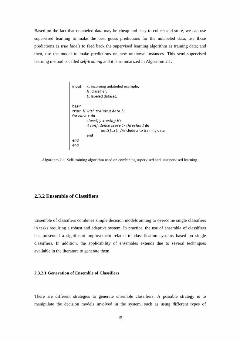
Based on the fact that unlabeled data may be cheap and easy to collect and store, we can use

supervised learning to make the best guess predictions for the unlabeled data; use these

predictions as true labels to feed back the supervised learning algorithm as training data; and

then, use the model to make predictions on new unknown instances. This semi-supervised

learning method is called self-training and it is summarized in Algorithm 2.1.

Algorithm 2.1. Self-training algorithm used on combining supervised and unsupervised learning.

2.3.2 Ensemble of Classifiers

Ensemble of classifiers combines simple decision models aiming to overcome single classifiers

in tasks requiring a robust and adaptive system. In practice, the use of ensemble of classifiers

has presented a significant improvement related to classification systems based on single

classifiers. In addition, the applicability of ensembles extends due to several techniques

available in the literature to generate them.

2.3.2.1 Generation of Ensemble of Classifiers

There are different strategies to generate ensemble classifiers. A possible strategy is to

manipulate the decision models involved in the system, such as using different types of

𝑡𝑟𝑎𝑖𝑛 𝐻 𝑤𝑖𝑡ℎ 𝑡𝑟𝑎𝑖𝑛𝑖𝑛𝑔 𝑑𝑎𝑡𝑎 𝐿;

input: 𝑥: incoming unlabeled example; 𝐻: classifier; 𝐿: labeled dataset;

begin

for 𝑒𝑎𝑐ℎ 𝑥 do 𝑐𝑙𝑎𝑠𝑠𝑖𝑓𝑦 𝑥 𝑢𝑠𝑖𝑛𝑔 𝐻; if 𝑐𝑜𝑛𝑓𝑖𝑑𝑒𝑛𝑐𝑒 𝑠𝑐𝑜𝑟𝑒 > 𝑡ℎ𝑟𝑒𝑠ℎ𝑜𝑙𝑑 do

𝑎𝑑𝑑(𝐿, 𝑥); //include 𝑥 to training data end

end end

16

classifiers (Ruta & Gabrys, 2005), different architecture of classifiers (Ruta & Gabrys, 2007),

and different initialization parameters (Altinçay, 2007).

Another possible strategy is to manipulate the data used. For instance, using different data

sources, different pre-processing techniques, different methods of sampling, among others. It is

important to say that the generation of ensemble of classifiers is mainly defined by the classifier

members and how to combine their decisions by means of a combining function.

In this way, we call by homogeneous, the ensemble classifiers composed by the same base

learners created with different model parameters; and heterogeneous, ensembles composed by

different base learners. We describe here the four most common methods used in the literature

to generate ensemble classifiers, precisely bagging, boosting, randomization and stacking.

• Bagging (Bootstrap AGGreatING): proposed by Breiman (1996) aiming to produce

several decision structures. It generates different data subsets of the same size from the

original training dataset. Each training dataset may get two or more copies of the same

instances, which provide diversity to the ensemble. This strategy is very suitable for

machine learning algorithms called "unstable". According to Breiman (1996), unstable

learning algorithms are the ones where any variation in the incoming data leads to huge

changes in the model.

• Boosting: different decision models are generated by different training subsets, as in

Bagging. However, Boosting is an iterative algorithm, where new classifiers are

influenced by the output from previous classifiers. The change in the training data

distribution for the new models is based on the misclassified instances by previous

models. In this way, Boosting try to improve the performance of each new model. It is

intuitive that each new model becomes an "expert" for instances that were misclassified

by all the previous models.

• Random subspace: proposed by Ho (1998), one randomly selects 𝑟 features (subspace)

from the 𝑝-dimensional dataset to construct each classifier, where 𝑟 < 𝑝. The ensemble

final decision is a combination of individual classifiers’ decisions, such as a simple

majority voting rule. This method may be used for both constructing and aggregating

classifiers.

• Stacking: this technique presents different base learners whose outputs are combined by

a meta-learner. We can say that the base learners are the level-0 models, and the meta-

learner is the level-1 model. The outputs of the different experts (base learners) are

input for the meta-learner, which presents better performance.

17

2.3.2.2 Combining Member Decisions

There are two popular solutions to combine individual decisions of ensemble members: fusion

and selection. (1) Fusion focus on providing an ensemble consensus by employing some rule,

such as majority vote; whilst (2) Selection chooses the most competent member of the ensemble

to classify the next incoming example.

Fusion assumes that ensemble members make decisions independently, i.e., they classify

different examples in different ways. The idea is to combine individual results in order to

improve the performance of the prediction (Kittler et al, 1998). However, in most real-world

problems, this assumption cannot be verified. In this case, there are no guarantees that ensemble

of classifiers will present higher performance than a single classifier (Smits, 2002). In the

literature, there are several combination rules, such as: majority voting, maximum rule,

minimum rule, median rule, naive bayes, among others.

Selection assumes the assumption that each classifier member is an expert in some regions of

competence of the problem (Parikh, 2007)(Zhu et al, 2004). We call the selection static or

dynamic whether the regions of competence are defined during the training phase or for the new

unknown sample, respectively. Since dynamic selection chooses an expert for every incoming

data, it may be a useful strategy to adapt the system given a concept drift occurrence, which is

investigated in this work.

2.3.2.3 Dynamic Classifier Selection

A framework for dynamic selection of classifiers is usually divided into 3 steps: 1) classifier

generation; 2) definition of regions of competence; and 3) dynamic selection. The first step is

executed using any generation method mentioned above, such as bagging and boosting, in order

to create an initial ensemble of classifiers. The second step focus on generating regions of

competence by using a training or a validation datasets, since the assumption here is that each

ensemble member is an expert in some regions of competence. The final step uses some

mechanism to choose the most competent member to classify the unknown examples. Precisely,

in dynamic selection, a region of competence is defined for each unknown instance individually

and the most competent classifier for that region is selected to assign the label to the unknown

instance.

18

Woods et al (1997) proposed a method called DCS-LA (Dynamic Classifier Selection with

Local Accuracy). In this method, the authors use a heterogeneous ensemble composed by five

classifiers. Basically, the method determines the 𝐾 nearest neighbors of the current example 𝑥

to evaluate the accuracy of the classifier members. Finally, the most accurate member is used to

classify 𝑥. A very similar method, proposed by Giacinto & Roli (2000), also determines the 𝐾

nearest neighbors to 𝑥, the difference is that their similarity must be higher than a specified

threshold.

Kuncheva (2000) proposed a method based on clustering and selection. The ensemble was

composed by MLP (MultiLayer Perceptrons) with different number of nodes in the hidden

layer. This method works as follows: clusters are generated using a training or a validation set.

Then, the cluster whose centroid is nearest to 𝑥 is chosen as 𝑥’s neighborhood. Finally, similar

to the methods previously described, the most accurate member over the 𝑥’s neighborhood is

used to classify it.

All the works mentioned in this section determine a neighborhood for the current example. In

general, these methods use validation dataset and an algorithm to calculate the 𝐾 nearest

neighbors of the instance. Especially noteworthy is the fact that the size of the validation dataset

may critically affect the performance of the ensemble based on local accuracy, which may be a

drawback to using this kind of solution for online systems.

2.4 Generic Solutions for Data Stream Problems

The generic solutions available in the literature for classification problems with concept drift

may be divided into different categories. It is important to know these categories to better

understand the methods used to handle concept drift. Such a diversity of approaches is due to

the different aspects taken into account, for instance: incoming data, number of classifiers,

incremental or non-incremental learning, and active or passive strategies.

2.4.1 Incoming Data

In real-world problems, the environments are non-stationary and the data arrive sequentially

over time, i.e., in a stream of data. For example, in environmental monitoring, online video

19

frames may be the data that arrive sequentially to the system. In this context, the first

categorization of approaches takes into account the organization of the input data, which can be

based on stream or batches. This choice depends on the velocity that the data are acquired and

the framework employed to make decisions. In data streams, the complexity of the problem

increases due to the high velocity and amount of input information provided to the system, in

addition to massive storage capacity requirements. Therefore, these dynamic environments often

require fast and real-time responses, besides constraints on memory usage and testing time.

There are windowing techniques, which are frequently used to handle concept drift in these

cases. They provide a mechanism of forgetting to select the new examples to train the classifier,

thus eliminating examples, which came from old concept distribution. One of the most common

windowing techniques is the sliding windows. This method selects the most recent examples to

train the classifiers.

The literature has shown that window size is the key issue for employing classifier windowing

techniques successfully, since using windows of fixed size can be a dilemma. On the one hand,

small windows of examples will allow quick reaction to changes, but it often causes

misdetection, leading to accuracy reduction in period of stability. On the other, large windows

of examples may contain data from different concepts, making the adaptation to new concepts

slower. As a consequence, large windows-based techniques often fail to adapt to sudden drifts

(Brzezinski & Stefanowski, 2014).

Classification systems trained using batches of examples over time are more prone to concept

drift. Besides, these systems may face other substantial problem, the so-called Catastrophic

Forgetting. This problem arises when classification systems learn new concepts, leading old

useful information being forgotten. As mentioned in Section 2.2, in real applications some

concepts can appear and disappear repeatedly. According to Chen et al (2012), the consequence

of ignoring old useful information can be catastrophic.

2.4.2 Number of Classifiers

Another way to divide robust solutions to deal with concept drift is based on the number of

classifiers used to make a decision: ensemble of classifiers or single classifiers. Generally,

handling concept drift using single classifiers is not very effective especially due to the

following two reasons. First, after training a classifier, its knowledge will not adapt to changes

unless the classifier is retrained. Second, if the classifier is retrained after each time period, it

20

will forget the previously learned concepts, which may lead to catastrophic forgetting,

especially when the environment presents recurring changes. Hence, traditional single classifiers

are feasible only on static environment problems.

Classifier ensembles have been successfully applied to cope with data streams problems. Rather

than designing a new robust and well-adapted classifier, an ensemble of classifiers can be used

to increase the system power of decision. According to the literature, classifier ensembles have

presented significant performance improvements when compared to classification systems

based on single classifiers. In studies like (Altinçay, 2007) (Tremblay et al, 2004) (Zhang et al,

2008) (Valentini, 2003) (Ruta & Gabrys, 2007), the authors conclude that ensembles of kNN (k-

Nearest Neighbors), SVM (Support Vector Machine) and Neural Networks present superior

performances than single kNN, SVM and Neural Network, respectively.

Concept drift detection using ensemble of classifiers based on labeled data can make use of

different window sizes, thresholds or heuristics. For example, we can use the nearest mean

classifier and update it with new observations without any forgetting, as proposed by Kuncheva

(2008). The details of some solutions using ensemble of classifiers are presented in the next

Chapter.

2.4.3 Incremental Learning x Non-Incremental Learning

This third categorization takes into account whether or not the data are reutilized. Incremental

learning has focused on sequential data processing (stream or batch) and cannot pass by the

same examples more than once (Ditzler & Polikar, 2013). Otherwise, it is considered non-

incremental.

In this context, Kuncheva (2004) affirms that the term incremental learning can be also called

online learning, whose definition is: data stream processing with constraints of runtime and

memory capacity to improve computational systems.

Minku & Yao (2012) advocate that online learning is useful for applications dealing with

streams of data, and they adopt the following definition for it: online learning algorithms

process each training example once, without the need of storage or reprocessing. The decision

model makes a prediction when an example becomes available, allowing the system to learn

from the example and to update the learning model. This definition adopted by Minku & Yao

21

(2012) for online learning is termed by Ditzler & Polikar (2013) as one-pass learning, but using

batch training data.

Hence, online learning may be considered a particular case of incremental learning. Moreover,

the latter refers to learning machines that are also used to model continuous processes, but also

deals with incoming data in chunks, instead of having to process each training example

separately. In this way, one-pass learning is also another particular case of incremental learning,

while learning methods that require access to previous data cannot be considered incremental.

Finally, we conclude that incremental learning, including both online and one-pass learning,

uses every incoming example to updates the system, even though the examples are processed in

chunks or separately.

2.4.4 Blind Strategy x Active Strategy

Finally, this approach divides the concept drift solutions into blind and active strategies, based

on whether or not a drift detection mechanism is employed as a component of the solution. The

idea of blind strategies is to update the system constantly using new input data without detecting

changes. We can say that the detection mechanism is implicit in the method.

Some solutions based on ensemble classifiers use dynamic combination rules and heuristics of

disposal of learning to always keep the system updated. For instance, (Zhang et al,

2008)(Rodríguez & Kuncheva, 2008)(Karnick et al, 2008)(Muhlbaier et al, 2009) proposed to

assign weights to each classifier member based on its previous performances. Thus, the

ensemble classifier members with the highest classification performances get the highest

weights when combined to obtain the final decision.

The main disadvantage of blind strategies is the computational cost involved, using ensemble

classifiers or not. Since the system updates constantly, even if changes do not occur, this may

lead to increase processing time by updating the system unnecessarily. An alternative to blind

strategies is to use active strategies, which explicitly employ detection mechanism. In this

context, the system adapts its knowledge to new information only after it perceives environment

changes.

22

2.5 Discussion

In this chapter we have presented some concepts and definitions related to our research. It has

been observed that concept drift is a problem that may affect different applications in different

ways, due to the diversity of possible drifts. In the context of solutions for the problem of

concept drift, it has been shown that these solutions may be divided according to some aspects,

such as: incoming data, number of classifiers, etc. These solutions may also be categorized into

supervised, unsupervised and semi-supervised methods, as the literature review related to our

work detailed in the next Chapter. Then, the two methods proposed in this work for handling

different types of changes are presented in Chapter 4 and Chapter 5.

23

Chapter 3

Related Work

This chapter presents a literature review on studies whose focus is on handling concept drift.

Taking into account that we propose in this work two methods to deal with concept drift, one

unsupervised and another semi-supervised, we divided these studies into three categories:

supervised methods, which include active strategies, called here drift detectors and blind

methods; unsupervised and semi-supervised methods. Drift detectors and blind methods are

described first. Then, unsupervised and semi-supervised methods are discussed.

3.1 Supervised Methods

These methods use fully labeled data to compose their mechanism to deal with concept drifts,

and are divided into two subcategories. This categorization takes into account whether or not

drifts are explicitly or implicitly detected, drift detectors (whose strategy is often based on error

monitoring) and blind methods (whose strategy is often based on periodical updates)

respectively.

24

3.1.1 Drift Detectors

Drift detectors compose a category of methods that utilizes statistical tests to monitor the class

distribution over time and to reset the decision model when a concept drift is detected. Based on

the definitions presented in the previous chapter, these methods are active strategies. We present

three drift detectors based on single classifiers and one drift detector based on ensemble

classifiers. All drift detectors discussed here update the decision model after drift detection.

The most popular drift detector is called Drift Detection Method (DDM), proposed by Gama &

Castillo (2006). This algorithm detects drifts based on online classification error rate motivated

by probably approximately correct (PAC) learning model (Mitchell, 1997). PAC assumes that,

if the distribution of the examples is stationary, the error rate of the learning algorithm will

decrease as the number of examples increases. Thus, an increase of this error rate suggests a

change in class distribution, leading the current model to be outdated.

DDM uses statistical tests to calculate the prequential error. The prequential error is the average

error obtained by the prediction of each incoming example, calculated in an online way (Dawid

& Vovk, 1999). The rule used to obtain the prequential error on time step 𝑡 is presented in the

Equation 3.1. Where 𝑒𝑟𝑟𝑒𝑥 is 0 if the prediction of the current example 𝑒𝑥 is wrong and 1 if it is

correct; and 𝑛𝑢𝑚𝑒𝑥 is the number of incoming examples until time step 𝑡.

𝑒𝑟𝑟(𝑡) = 𝑒𝑟𝑟(𝑡 − 1) + 𝑒𝑟𝑟𝑒𝑥(𝑡) − 𝑒𝑟𝑟(𝑡 − 1) 𝑛𝑢𝑚𝑒𝑥⁄ (3.1)

DDM defines two thresholds, called warning level and drift level, which are reached if

conditions (Equation 3.2) or (Equation 3.3) are satisfied, respectively. The 𝑝 value represents

the prequential error rate of the learning algorithm, while 𝑠 denotes its standard deviation. The

registers 𝑝𝑚𝑖𝑛 and 𝑠𝑚𝑖𝑛 are set during the training phase, and are updated if after each incoming

example (𝑖) the current register 𝑝𝑖 + 𝑠𝑖 is lower than 𝑝𝑚𝑖𝑛 + 𝑠𝑚𝑖𝑛.

𝑝𝑖 + 𝑠𝑖 ≥ 𝑝𝑚𝑖𝑛 + 2 ∗ 𝑠𝑚𝑖𝑛 (3.2)

𝑝𝑖 + 𝑠𝑖 ≥ 𝑝𝑚𝑖𝑛 + 3 ∗ 𝑠𝑚𝑖𝑛 (3.3)

25

For instance, given that the error rate of the current model reaches the warning level at example

𝑘𝑛, while the drift level is reached at example 𝑘𝑝, in DDM, it is assumed that the concept

changes at 𝑘𝑝 and a new context is declared between 𝑘𝑛 and 𝑘𝑝. In the adaptation process, the

new decision model should be generated using only the new context, i.e., the same classifier is

retrained using examples stored between 𝑘𝑛 and 𝑘𝑝.

The main drawback to this strategy is that the velocity of the changes critically affects DDM.

Consequently, if a very slow gradual change takes place, the system will not be able to detect it.

In order to overcome this drawback, Baena et al (2006) proposed the Early Drift Detection

Method (EDDM). The basic idea of EDDM is that the distance between two consecutive errors

will increase by improving the predictions of the decision model. Similar to DDM, two

thresholds are defined when using EDDM, also called warning level and drift level.

EDDM calculates the distance (𝑝′) between two consecutive errors and their standard deviation

(𝑠′), and stores the maximum values of 𝑝′ and 𝑠′ to register the point where the distance between

two errors is maximum(𝑝′𝑚𝑎𝑥 + 2 ∗ 𝑠′𝑚𝑎𝑥). According to Baena et al (2006), the warning level

is reached when the Equation 3.4 is lower than α (they set α to 0,95), and the drift level is

reached when the same Equation 3.4 is lower than β (they set β to 0,9).

(𝑝′𝑖 + 2 ∗ 𝑠′𝑖)/(𝑝′𝑚𝑎𝑥 + 2 ∗ 𝑠′𝑚𝑎𝑥) (3.4)

Here, however, the thresholds must be used to monitor the decrease on the distance between two

errors. And also, the adaptation process is basically the same as used in DDM, i.e. the decision

model is updated using only the new context, ranging from warning and drift levels.

EDDM starts the search for concept drifts after calculating 30 classification errors, due to the

fact that the authors intended to estimate the distance distribution between two consecutive

errors in order to compare it with further distributions. The results attained by EDDM were

better than the results provided by DDM in some databases. In addition, EDDM was able to

detect gradual changes earlier even when the changes were very slow. Even though, EDDM was

not robust enough to noisy datasets.

Another popular drift detector was proposed by Nishida & Yamauchi (2007), called Detection

Method Using Statistical Testing (STEPD), which is based on two accuracies: the recent one

and the overall one. The recent accuracy is calculated for a recent set of examples, called 𝑊,

26

while the overall accuracy is calculated for the whole set of examples from the beginning of

learning, except for the recent 𝑊 examples. STEPD relies on two assumptions: (a) if the

accuracy of a classifier for recent 𝑊 examples is equal to the overall accuracy, then the target

concept is stationary; (b) a significant decrease on recent accuracy suggests concept drift.

STEPD compares the statistic 𝑇 presented in Equation 3.5 to the percentile of standard normal

distribution to obtain the observed level (𝑃) of significance, and defines two levels of

significance as thresholds. In order to better clarify the comparison among drift detectors, we

also call these two levels of significance as warning and drift levels. The algorithm starts by

storing examples when 𝑃 is lower than the warning level, and retrain the classifier when 𝑃 is

lower than the drift level. The classifier retraining is conducted using examples stored between

both levels.

𝑇(𝑟𝑜𝑟𝑟𝑛𝑜𝑛𝑟) =|𝑟𝑜 𝑛𝑜⁄ −𝑟𝑟 𝑛𝑟⁄ |−0.5(1 𝑛𝑜⁄ +1 𝑛𝑟⁄ )

√𝑝(1−𝑝)(1 𝑛𝑜⁄ +1 𝑛𝑟⁄ ) (3.5)

Here, 𝑟𝑜 is the number of correct classifications considering overall examples (𝑛𝑜), except the

recent 𝑊 examples, 𝑟𝑟 is the number of correct classifications among 𝑊 examples (𝑛𝑟), and

�̂� = (𝑟𝑜 + 𝑟𝑟)/(𝑛𝑜 + 𝑛𝑟).

According to Nishida & Yamauchi (2007), in comparison to EDDM and DDM, STEPD

presented the highest performances for abrupt changes and noises. However, EDDM detected

gradual changes better than STEPD, while DDM well detected abrupt changes, but its detection

speed was the slowest one.

These supervised-based methods summarized so far have focused on dealing with concept drift

by explicitly detecting drifts using single classifiers. However, as mentioned in Chapter 2,

approaches based on single classifiers may be prone to catastrophic forgetting. An alternative to

these previous methods is to use drift detectors combined with classifier ensembles to react to

drifts more quickly.

Following this idea, Minku & Yao (2012) proposed the Diversity for Dealing with Drift (DDD).

This method processes each example at a time and maintains ensembles with different diversity

levels in order to deal with concept drift. Basically, DDD generates a pool of classifiers using a

modified version (Minku & Yao, 2010) of online bagging (Oza & Russell, 2001), as follows.

Whenever a training example is available, it is presented 𝑁 times for each base learner, and the

classification is performed by weighted majority vote, as in offline bagging. Then, the classifier

27

members are separated into two subsets of classifiers: (1) low diversity; and (2) high diversity

ensembles.

It is important to note that there is no generally accepted formal definition of diversity yet. The

researchers are still investigating how diversity should be measured and what means this

measure. Johansson et al (2007) suggest that diversity is almost an axiom based on the

assumption that classifier members must be diverse to assure that an ensemble will more likely

present good generalization. Since there is no consensus about which proposed diversity

measure is the best one, DDD measures diversity using Q statistic, recommend by Kuncheva &

Whitaker (2003), due to its simplicity and easy interpretation. Minku & Yao (2012) consider

that high/low diversity refers to high/low average Q statistic.

The aim of using high/low diversity ensembles is the assumption that the accuracy of the

ensembles may be similar (not the same) or very distinct, according to the severity and the

speed of each type of drift. For instance, the authors observed that high diversity ensembles

achieve better accuracy rates when dealing with low severity and high speed drifts.

DDD operates in two modes: before and after drift detection. In the first mode, the low diversity

ensemble and the high diversity ensemble are generated using incoming examples. Then, the

after drift detection mode is triggered when there is no convergence about the concept. DDD

monitors the low diversity ensemble using a drift detector, namely EDDM. In this last mode, the

low/high diversity ensembles generated in the first mode are assigned as old low/high diversity

ensembles and the first mode is reactivated in order to create new low/high diversity ensembles.

In general, DDD aims to learn new concepts using the information learned from the old

concepts, i.e., by training the old high diversity ensemble on new concept, allowing its diversity

to be lower. Minku & Yao (2012) have presented experiments using artificial and real-world

data to show that DDD usually achieves similar or even better accuracy than EDDM.

3.1.2 Blind Methods

Aside the drift detectors, there is a category of blind methods which update their knowledge

base by adding, removing or updating classifiers periodically. As mentioned in the previous

chapter, these methods are also called passive strategies. Many blind solutions using ensemble

of classifiers have been proposed to handle concept drift in online and incremental learning

28

contexts. In these solutions, each example can be processed separately or in chunks (blocks of

data).

Some of the most known algorithms based on ensemble classifiers utilize the passive strategy to

build ensembles by adding members using every incoming data and removing members by

employing different strategies: removing the oldest member, e.g. Streaming Ensemble

Algorithm (SEA)(Street & Kim, 2001); or removing the poorest performing member to be

replaced by a new classifier, such as Dynamic Weighted Majority (DWM)(Kolter & Maloof,

2007) and Learn++NSE for NonStationary Environment (Muhlbaier & Polikar, 2007).

For instance, the Learn++NSE method trains a new classifier for every incoming chunk of data.

Thus, a performance monitoring mechanism is conducted using new and old data. Then, the

average error is combined to majority voting to determine a voting weight to each classifier. In

this way, the poorest performing classifier on the current concept is discarded. Another example

is the SEA method, which trains a new classifier for every incoming chunk of data and increases

or decreases the quality of its classifiers based on accuracy. This method removes the oldest

member in a fixed-size ensemble.

Based on DWM strategy, Sidhu et al (2013) proposed a novel online ensemble approach called

Early Dynamic Weighted Majority (ERDWM). The weighted strategy is undertaken using three

options: (1) decreasing the weight of members whose local prediction is incorrect; (2)

increasing the weight of members whose local prediction is correct but global prediction is

incorrect; and (3) no performing weight update when both local and global predictions are

correct.

ERDWM focus on the highest performing classifier members in order to reduce the chances of

incorrect global prediction, main problem detected in DWM. In addition, ERDWM reduces the

need of creating new classifier members and consequently, it decreases time and memory

resources requirements. Even though, Sidhu et al (2013) conclude that ERDWM does not

outperform EDDM in terms of memory and execution time. On the other hand, ERDWM is

better in maintaining previous knowledge to aid making predictions.

Another work using passive strategy is presented by Brzezinski & Stefanowski (2014). They

propose a method called Accuracy Updated Ensemble (AUE2), which combines the principles

of chunk-based ensemble with incremental-based components and it presents a mechanism to

achieve high predictions in occurrence of different types of drift at relatively low computational

costs. In AUE2, a new ensemble classifier member is created after each incoming data chunk of

examples and it replaces the poorest performing member. The remaining ensemble members are

29

updated according to their accuracy. The weighting calculated according to Equation 3.6 is used

to combine information about the accuracy of classifiers and the current class distribution.

𝜔𝑖𝑗 =1

𝑀𝑆𝐸𝑟+𝑀𝑆𝐸𝑖𝑗+𝜖 (3.6)

where 𝑀𝑆𝐸𝑖𝑗 denotes the estimate of the error prediction of each classifier on each data chunk,

while the value of 𝑀𝑆𝐸𝑟 is the mean square error of a randomly predicting classifier and is used

as a reference point to the current class distribution. Moreover, ϵ denotes a small positive value

added to avoid the division by zero problem. Equation 3.5 is used to update the weight of the

remaining classifier members.

In addition, in (Brzezinski & Stefanowski, 2014), the authors assume that the most recent

incoming data chunk (𝐵𝑖) is the best representation of the current and near-future data

distribution. This way, a classifier 𝐶′, trained on 𝐵𝑖, is treated as the best possible (or perfect)

classifier and its weight is assigned by Equation 3.7.

𝜔𝐶′ =1

𝑀𝑆𝐸𝑟+𝜖 (3.7)

According to the authors, AUE2 achieves higher classification accuracy than its predecessors

(Accuracy Weighted Ensemble - AWE and SEA) in the presence of slow gradual drifts.

Besides, ensemble members can be retrained, which makes AUE2 less dependent on chunk size

and it allows using smaller chunks without compromise its accuracy. Finally, to solve the

problem of memory usage, AUE2 sets a memory usage limit (threshold) that, when exceeded,

decreases the size of classifier members.

A recent framework proposed by (Almeida et al, 2016), called Dynamic Selection Based Drift

Handler (DYNSE), uses dynamic ensemble selection to choose an expert subset of classifiers to

assign a label to an incoming instance. DYNSE intends to deal with concept drift by building a

new classifier using every most recent incoming data, organized in batches of samples, which

are also used to replace a validation dataset at each update. Instead of discarding the oldest

classifiers as classical methods do, DYNSE is designed to keep as much classifier members as

possible. When a new instance x arrives, this method works as follows: a region of competence

30

is identified as the set of k nearest neighbors over samples contained in a validation dataset

surrounding x. Then, a subset of classifiers is dynamically selected to predict the x’s label. Even

using dynamic selection of classifiers, this method is in the category of blind methods based on

supervised learning, since it is assumed that the method receives a large enough batch of

supervised instances every month to adapt the system.

3.2 Unsupervised Methods

Different from the strategies mentioned before, this category of methods intends to handle

concept drift even if only unlabeled data are available. In such a context, there are many data

stream problems, which have only unlabeled data to be dealt with. In this section, some

unsupervised strategies are described.

The method proposed by (Fanizzi et al, 2008), is applicable in two problems: concept drift

(change of known concepts) and novelty detection (change of unknown concept). An isolated

cluster in the search space represents this last problem. In their method, samples are divided into

clusters. The maximum distance between clusters’ instances and medoids is computed to

establish a decision boundary for each cluster. The union of the boundaries of all clusters is

called global decision boundary. The new unseen incoming examples that fall outside this

global decision boundary are not considered “normal” and need a further analysis. In this way,

these examples are stored in a short-term memory for grouping new clusters, which might

indicate concept drift or novelty detection.

Another work based on dissimilarity measures between data employed to detect concept drift is

found in (Otey & Parthasarathy, 2005). In this work, the authors calculate the dissimilarity

between two windows (�̅� and �̅�) considering three components: distance, rotation and variance.

For the distance component, its dissimilarity 𝐷𝑑𝑖𝑠𝑡 is computed by means of Euclidean distance

between the centroids of each dataset (µ�̅� and µ�̅�), according to Equation 3.8:

𝐷𝑑𝑖𝑠𝑡(�̅�, �̅�) = |µ�̅� − µ�̅�| (3.8)

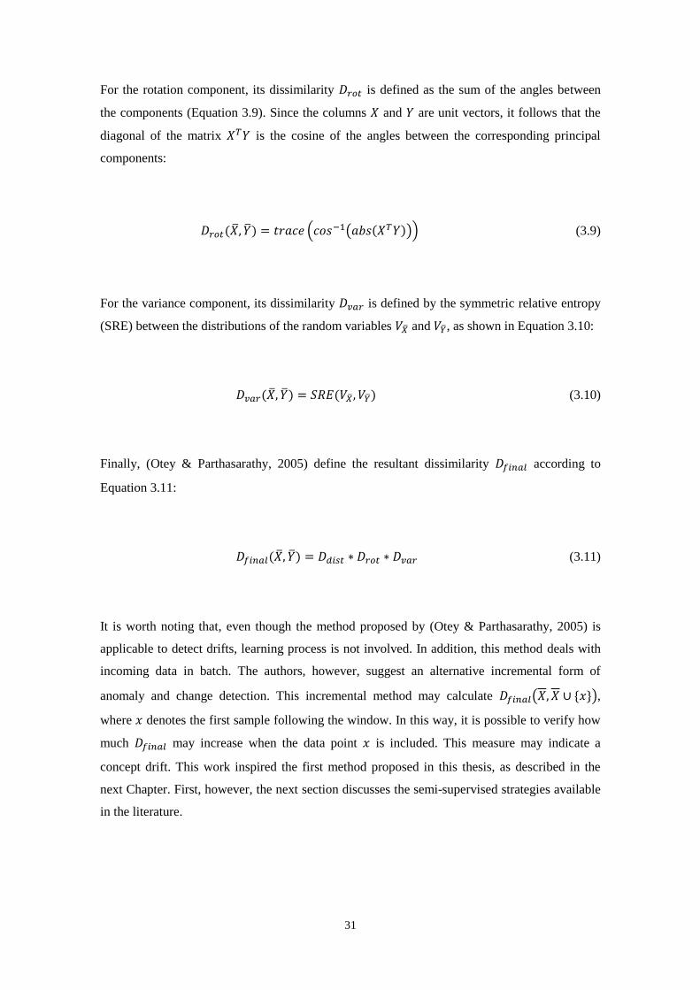
31

For the rotation component, its dissimilarity 𝐷𝑟𝑜𝑡 is defined as the sum of the angles between

the components (Equation 3.9). Since the columns 𝑋 and 𝑌 are unit vectors, it follows that the

diagonal of the matrix 𝑋𝑇𝑌 is the cosine of the angles between the corresponding principal

components:

𝐷𝑟𝑜𝑡(�̅�, �̅�) = 𝑡𝑟𝑎𝑐𝑒 (𝑐𝑜𝑠−1(𝑎𝑏𝑠(𝑋𝑇𝑌))) (3.9)

For the variance component, its dissimilarity 𝐷𝑣𝑎𝑟 is defined by the symmetric relative entropy

(SRE) between the distributions of the random variables 𝑉�̅� and 𝑉�̅�, as shown in Equation 3.10:

𝐷𝑣𝑎𝑟(�̅�, �̅�) = 𝑆𝑅𝐸(𝑉�̅�, 𝑉�̅�) (3.10)

Finally, (Otey & Parthasarathy, 2005) define the resultant dissimilarity 𝐷𝑓𝑖𝑛𝑎𝑙 according to

Equation 3.11:

𝐷𝑓𝑖𝑛𝑎𝑙(�̅�, �̅�) = 𝐷𝑑𝑖𝑠𝑡 ∗ 𝐷𝑟𝑜𝑡 ∗ 𝐷𝑣𝑎𝑟 (3.11)

It is worth noting that, even though the method proposed by (Otey & Parthasarathy, 2005) is

applicable to detect drifts, learning process is not involved. In addition, this method deals with

incoming data in batch. The authors, however, suggest an alternative incremental form of

anomaly and change detection. This incremental method may calculate 𝐷𝑓𝑖𝑛𝑎𝑙(𝑋, 𝑋 ∪ {𝑥}),

where 𝑥 denotes the first sample following the window. In this way, it is possible to verify how

much 𝐷𝑓𝑖𝑛𝑎𝑙 may increase when the data point 𝑥 is included. This measure may indicate a

concept drift. This work inspired the first method proposed in this thesis, as described in the

next Chapter. First, however, the next section discusses the semi-supervised strategies available

in the literature.

32

3.3 Semi-supervised Methods

Even though unsupervised drift detectors are assumed to be the solution for dealing with fully

unlabeled data, these methods must assume some structure to the underlying distribution of

data, must store clusters in a short-term memory and their decisions depend on

similarity/dissimilarity measures. All these aspects may compromise system performances in

online practical problems. In order to avoid storing examples and to provide more confident

decision models, semi-supervised methods may be an interesting alternative since they usually

allow working with a small amount of labeled data and a large amount of unlabeled data.

Wu et al (2012) proposed the SUN (Semi-supervised classification algorithm for data streams

with concept drifts and UNlabeled data). Basically, SUN divides the streaming data into two

sets: training and testing dataset. First, at the training phase, the method builds a growing

decision tree incrementally and generates concept clusters in the leaves using labeled

information. The unlabeled data are labeled according to the majority-class of their nearest

cluster. Then, SUN suggests a concept drift based on the deviation measured in terms of

distance, radius, etc., between old and new concept cluster. Secondly, at the test phase, the

examples are evaluated using the current decision tree.

However, SUN searches for concept drifts only during the training phase, where samples

contained in the training set are assigned to true labels or to pseudo-labels. During the test

phase, the method assumes that all concepts described in the data stream are already known.

Moreover, in terms of drift detection, the results attained by SUN are worse than its baseline,

since SUN produces more false detections, missing detections and larger delays of drift

reactions.

Another semi-supervised strategy for dealing with concept drift in the context of data streams

was proposed by Kantardzic et al (2010). Here, however, instead of using single classifiers, the

authors employed ensemble of classifiers. Their online method calculates similarity measures to

select suspicious examples, which are assumed to belong to the new concept. Suspicious

examples are samples that must be labeled in order to improve the accuracy of the current

classifier. The incoming streaming examples are clustered in the current distribution and the

suspicious examples are put together to form the new regions. This method does not build a new

classifier for the ensemble periodically and it also does not detect the moment when drifts occur.

The system update works as follows: when the number of examples assigned to a cluster new

region reaches the predefined minimum number of examples, the ensemble requests a human

33

expert to label them. After such a labeling process, the ensemble builds a new member classifier

and removes the oldest one.

One more recent semi-supervised method based on ensemble classifiers is called SAND (Semi-

Supervised Adaptive Novel Class Detection and Classification over Data Stream) proposed by

Haque et al (2016). SAND maintains a window W to monitor estimates of classifier confidence

on recent data instances. It means that a decreasing of classifier confidence suggests a concept

drift. In order to update the ensemble, SAND uses the recent chunk and selects some instances

(by classifier confidence) to be labeled and to be included in the training dataset for a new

model (which replaces the oldest one). In this way, SAND deals with the concept drift problem

updating the ensemble always with the most recent concept.

3.4 A Comparative Analysis of the Current Methods

All methods described in this chapter are listed in Table 3.1. This table highlights how these

methods are divided according to the approach of generic solutions presented in Chapter 2. In

addition, Table 3.1 also shows the type of changes that each method intends to deal with.

Finally, for drift detectors, the measure used for drift detection is mentioned too.

DDM, EDDM and STEPD represent the same configuration of approaches. The main difference

between these three drift detectors is the statistical test employed. These methods are based on

single classifier, which is replaced after drift detection. Moreover, incoming data arrive in a

stream, updating the current decision model incrementally (online learning). When warning

level is reached, the samples update a kind of alternative decision model. However, alternative

model only replaces the current decision model when drift level is reached. Since DDM, EDDM

and STEPD pass by the same sample just once, these methods are assumed to be online.

We also consider DDM, EDDM and STEPD as active methods, since the drift detection is

explicit in their strategies. However, these methods include every incoming sample to the

decision models (current or alternative), i.e. the system does not update only after drift

detection. Actually, the system is updated as the incoming samples arrive. These methods are

robust at handling abrupt and gradual drifts. However, EDDM performs better when gradual

drifts are very slow because it is based on distance between error occurrences.

34

Table 3.1. Compilation of related work reported in literature grouped according to the approach of generic

solutions for dynamic environments problems.

Category Method Classifiers Learning Strategy Detection

based on Proposed to deal with

Drift

Detectors

DDM Single Online Active Error

monitoring

Abrupt/Gradual drifts

and noises

EDDM Single Online Active Error

monitoring

Abrupt/Gradual (slow)

drifts

STEPD Single Online Active Error

monitoring

Abrupt/Gradual drifts

and noises

DDD Ensemble Incremental Active

It depends on

detection

method used

Abrupt/Gradual (slow)

drifts and noises

Blind

Methods

SEA Ensemble One-Pass Blind - Abrupt drifts and

noises

Learn++NSE Ensemble One-Pass Blind - All drifts

DWM Ensemble Online Blind - Noises

ERDWM Ensemble Online Blind - Recurring concepts and

noises

AUE2 Ensemble One-Pass Blind - All drifts and noises

DYNSE Ensemble One-Pass Blind - All drifts and noises

Unsupervised

Methods

Fanizzi et al,

2008 Single One-Pass Active Dissimilarity -

Otey &

Parthasarathy

2005

- - Active Dissimilarity Abrupt drifts and blips

Semi-

Supervised

Methods

SUN Single Online Blind - All drifts and noises

Kantardzic et

al, 2010 Ensemble Online Blind - All drifts

SAND Ensemble One-Pass Active

Classifier

Confidence

Scores

All drifts

Our

Proposed

Methods

DbDDM Single Online Active Pseudo-error

monitoring All drifts

DSDD Ensemble Online Active Pseudo-error

monitoring All drifts

Blind methods based on ensemble classifiers are better in maintaining previous knowledge than

methods based on single classifier. Blind methods also use incremental learning divided into

online learning, when the incoming data arrive as stream (DWM, ERDWM and DDD), and one-

pass learning, when incoming data arrive as batch (SEA, AUE2 and DYNSE). Except for DDD,

all the methods based on ensemble classifiers mentioned in this chapter use passive strategies to

35

handle concept drifts. These methods are robust on reacting to new concepts. In addition, due to

the ensemble of classifiers, they are also robust on reacting to recurrent concepts. However, in

period of stable concepts, they remain updating the system unnecessarily.

In despite of the fact that DDD uses active strategy, this method needs an algorithm to detect

changes. However, as mentioned before, since the authors used EDDM only at the changing

detection phase, DDD is considered an incremental learning method, as shown in Table 3.1.

Besides, it is assumed that DDD is an incremental learning method because it allows choosing a

drift detector, which passes by each sample only once.

The unsupervised methods described in this chapter are based on clustering. In (Fanizzi et al,

2008), even though incoming data arrive on stream, first this method waits to form a cluster.

Then, it integrates the created cluster to the model. Since it presents explicit drift detection, this

method is assumed as an active strategy. The method proposed by Otey & Parthasarathy (2005)

is totally based on data distribution. Therefore, it does not use either a classifier or learning. In

addition, this method presents active strategy for data stream. It is better on detecting abrupt

drifts due to the fact that the change should occur from one window to another one. The

incremental form of change detection suggested by the authors may handle gradual drifts.

The semi-supervised methods mentioned in this work aim to update their systems to deal with

evolving data streams. They handle concept drifts by updating their systems using a small

selected amount of the most recent labeled examples. On the one hand, except for SAND, they

do not present high performance on detecting drifts at the right moments when they occur. On

the other, these semi-supervised methods present high accuracy rates and reduce the

computational cost of the labeling process.

In addition, most of the methods based on ensemble classifiers, in both blind and semi-

supervised categories, make their predictions by majority voting as ensemble fusion function.

DYNSE is an exception, since it makes predictions based on dynamic classifier selection.

Classifier fusion assumes error independence among ensemble’s component members. This

means that the classifier members are supposed to misclassify different patterns. In this way, the

combination of classifier members’ decision would improve the final classification

performance. However, when the condition of independence is no verified, there is no guarantee

that the combination of classifiers will outperform single classifiers (Kuncheva, 2002). In order

to avoid the assumption of independence of classifier members, methods for classifier selection

have been used as alternative to classifier fusion.

In order to achieve the objectives of this research, the blind methods are practically infeasible,

due to the following reasons. First, to be able to react to all changes, a system based on passive

36

strategy must be updated in short time intervals, leading to high computational cost. Second, if

the system is updated in large time intervals, some changes may not be noticed by the system.

These drawbacks allow us to believe that the best moment for system update is after change

detection. In this way, the system will not spend an unnecessary computational cost, and all

relevant changes will be noticed. Therefore, drift detectors may be considered better than blind

strategies, because they are based on explicit detection of changes.

In addition, as confirmed in this chapter, ensemble of classifiers achieves better performance on

handling many types of drifts, when compared to single classifiers. However, most of the

ensemble-based techniques available in the literature are blind strategies. The exception is

DDD. However, as mentioned before, this method needs a drift detector.

In terms of active methods, they are based on error monitoring, dissimilarity between incoming

data, or classifier confidence. Error monitoring-based methods need an operator feedback to

indicate if the error rate has increased, i.e., it is necessary to know the true labels of the whole

data. However, in stream data problems, the true labels are not always available. In this context,

the dissimilarity-based methods take advantage, due to the fact that they detect drifts on

unlabeled data and do not need to wait for error rate increasing to detect drifts. Even though,

these methods must assume some structure to the underlying distribution of data, must store

clusters in a short-term memory and their decisions depend on similarity/dissimilarity measures.

All these aspects may compromise system performances in online practical problems.

During the adaptation process, all systems described in this chapter follow a standard process:

drift detectors based on single classifiers replace the classifiers after drift detection using the

most recent data to update their models, while ensemble-based, for both active and passive

strategies, create new ensemble members using the most current data. What makes the

difference in the adaptation process of ensemble-based methods is the identification of the right

moment to replace old members, such as intended by Minku & Yao (2012) in DDD and Haque

et al (2016) in SAND.

Therefore, there are many open problems on employing classification systems to deal with

concept drift. In this work, we present two methods. Both proposed methods focus on detecting

drifts explicitly in an unsupervised way by monitoring a pseudo error and updating the decision

model just after drift detections. The estimation of the pseudo error is the main novelty of our

methods, since it allows simulating the most common supervised drift detectors to be also used

by unsupervised and semi-supervised methods.

37

Our two proposed methods (DbDDM and DSDD) are included in Table 3.1. All the details

about the configurations of these proposed methods, experiments and results are summarized in

the two next chapters.

38

Chapter 4

Dissimilarity-based Drift Detection

Method

This work intends to overcome the following drawbacks identified in the current methods for

data stream problems: classification error rate monitoring and unnecessary system updates. In

this way, in order to avoid detecting changes based on performance monitoring, we propose a

method to detect drifts by monitoring the dissimilarity between past and current data

distributions. The decision model is kept until drift detection to avoid unnecessary updates, i.e.

the model is reset to posterior incoming data as soon as a drift is detected. We call our method

Dissimilarity-based Drift Detection Method (DbDDM).

A conventional prediction system for stable concepts is used to start the system, when it is

necessary an initial decision model to predict every incoming sample. Thus, the unknown data

arrive in a stream toward DbDDM, which detects drifts based on dissimilarity between the

current sample and past data. It is important to mention that this past data represent small

clusters created by grouping the most recent past data, which are updated with every incoming

sample.

For the system reaction phase, as long as DbDDM does not alarm drift detection, the current

decision model keeps classifying the incoming samples. When a concept drift occurs, the

reference clusters are reset using the most recent incoming data. This chapter describes the

whole method in details, as well as the results attained by experiments conducted using artificial

and real datasets.

39

The proposed DbDDM may be included in the category of drift detectors, since it resets the

decision model when a concept drift is observed. DbDDM is divided into two modules: (1)

dissimilarity calculation; and (2) drift detection.

The first module is motivated by work (Otey & Parthasarathy, 2005). The authors advocate that

an incremental form of anomaly detection for data stream applications may be achieved by

calculating 𝐷(𝑾, 𝑾 ∪ {𝑋𝑖}), where 𝑾 is a sliding window of 𝑘 samples, 𝑋𝑖 is the first sample

following the window, and 𝐷 is the resulting dissimilarity measure. In our method, we

implement this incremental form of anomaly detection. It is important to mention that these

authors originally worked only with cluster of samples, i.e. they calculated 𝐷(𝑾, 𝒁), where 𝑾

and 𝒁 are both windows of data. Moreover, their method did not involve learning, i.e., their aim

was to identify whether or not 𝑾 and 𝒁 were significantly different.

The second module of DbDDM is inspired by DDM and EDDM using statistical process control

(SPC). As mentioned in the last chapter, DDM and EDDM are both incremental learning-based

and accuracy monitoring-based methods. Here, however, in order to avoid accuracy monitoring,

our method uses SPC to verify when the dissimilarity between the current unknown samples

and previous known data reaches the warning or the drift level.

DbDDM works as follows. First, a classifier is trained using samples contained in a training

dataset. Then, the training dataset is partitioned into c clusters, where c indicates the number of

classes, to be used as reference clusters. We call each group of class by cluster 𝐶𝑛. For instance,

two classes will result in two clusters: 𝐶1 and 𝐶2. Afterwards, the classifier will assign a label

for each new (unknown) sample 𝑋𝑖 one at a time, such as incoming data in a stream.

We extend the conventional prediction system to handle concept drift taking into account only

data distribution (Figure 4.1). The aim is to detect concept drifts by analyzing the dissimilarity

between the current sample and the reference clusters, and then to update the classifier to new

concept. Since our drift detector is based on SPC, it may be adaptable to any SPC statistical test.

We have employed the statistical tests performed in DDM and EDDM. In order to better

describe this overview scheme, we divided it into three sections: dissimilarity module; drift

detection module based on DDM; and drift detection module based on EDDM.

40

Figure 4.1. Overview scheme of the proposed method: It starts with every incoming example being

predicted by dissimilarity module. This dissimilarity prediction is compared to the classifier prediction by

the drift detection module in order to calculate when the assumed dissimilarity prediction error suggests a

concept drift.

4.1 Dissimilarity Module

The dissimilarity module may also be divided into two levels: (1) dissimilarity measurement;

and (2) cluster update. In the first level, for instance, given a 𝑛-classes problem, there are 𝑛

initial clusters (𝐶1, 𝐶2,..., 𝐶𝑛). For each incoming sample 𝑋𝑖, the method calculates its

dissimilarity to each cluster: 𝐷1(𝐶1, 𝐶1 ∪ {𝑋𝑖}), 𝐷2(𝐶2, 𝐶2 ∪ {𝑋𝑖}) up to 𝐷𝑛(𝐶𝑛, 𝐶𝑛 ∪ {𝑋𝑖}).

Afterwards, it is assigned to 𝑋𝑖 the class represented by the cluster less dissimilar to it. It is

important to mention that the dissimilarity measurement is considered as a parameter for this

module. Therefore, we used the measurements according to Equation 3.10, defined in the last

chapter, as proposed by (Otey & Parthasarathy, 2005). It is a combination of three components:

distance, rotation and variance.

As it can be observed, classification error is not taken into account at the first level. The second

level is devoted to update the reference clusters, which is conducted as follows: the real label of

𝑋𝑖 is verified, and 𝑋𝑖 is used to update the correct cluster by removing the oldest sample and

adding 𝑋𝑖. Therefore, the cluster update level is a supervised component of DbDDM.

41

It is important to say that the same initial clusters 𝐶𝑛 are used as input of the dissimilarity

module for the next sample and so on. Meanwhile, the class prediction by dissimilarity is used

as input for the next module: the drift detection module. We can observe all steps involved in

the dissimilarity module in Algorithm 4.1.

Algorithm 4.1. DbDDM Dissimilarity module algorithm.

4.2 Drift Detection Module based on DDM

The drift detection module receives two predictions to 𝑋𝑖 as input: the classifier prediction

(𝑃𝑟𝑒𝑑1), and the dissimilarity prediction (𝑃𝑟𝑒𝑑2). Precisely, 𝑃𝑟𝑒𝑑1 denotes the class assigned

by the classifier to sample 𝑋𝑖, while 𝑃𝑟𝑒𝑑2 denotes the class of the cluster less dissimilar to 𝑋𝑖.

It is important to mention that we do not evaluate whether or not the classifier made the right

decision on assigning the selected class to 𝑋𝑖. We assume that 𝑃𝑟𝑒𝑑2 is the reference to know if

𝑃𝑟𝑒𝑑1 is correct or wrong.

Given that 𝐶𝑟 is the cluster related to the class predicted in 𝑃𝑟𝑒𝑑2, when 𝐷𝑟(𝐶𝑟 , 𝐶𝑟 ∪ {𝑋𝑖}) is

lower than the average dissimilarity calculated by all dissimilarities in this concept (𝑚𝑒𝑎𝑛(𝐷)),

𝑃𝑟𝑒𝑑2 is considered a correct reference prediction. Otherwise, it is a wrong reference

prediction.

input: 𝑋𝑖: incoming stream sample;

RefClusters: set of k reference clusters;

output: 𝑃𝑟𝑒𝑑2: dissimilarity prediction;

𝐷𝑟: dissimilarity measure related to the class predicted in 𝑃𝑟𝑒𝑑2;

RefClusters: updated reference clusters;

begin

for 𝑒𝑎𝑐ℎ 𝐶𝑘 𝜖 RefClusters do 𝐷𝑘(𝑋𝑖 , 𝐶𝑘);

𝐷𝑟 ≔ min (𝐷); //lower dissimilarity measure

return 𝐶𝑘| min(𝐷); //cluster less dissimilar

𝑃𝑟𝑒𝑑2 ≔ 𝑐𝑙𝑎𝑠𝑠(𝐶𝑘| min(𝐷)); //class label predicted

RefClusters ≔ 𝑢𝑝𝑑𝑎𝑡𝑒(𝐶𝑘|𝑙𝑎𝑏𝑒𝑙(𝑋𝑖)𝜖 𝐶𝑘); //update based on true label

end

42

In this way, we use the prediction 𝑃𝑟𝑒𝑑2 in order to calculate the SPC based on a pseudo

prequential error 𝑝𝑖 with standard deviation given by: 𝑠𝑖 = √𝑝𝑖(1 − 𝑝𝑖)/𝑖. In our method, the

SPC (such as the dissimilarity measurements) is a parameter, i.e., it is possible to choose the

same statistical test used by DDM, EDDM, STEPD or any other method based on SPC.

To better understanding the method, here, we describe it using the SPC-based DDM. This

pseudo prequential error increases as 𝑃𝑟𝑒𝑑1 is considered incorrect by 𝑃𝑟𝑒𝑑2. Otherwise, 𝑝𝑖

decreases. On the one hand, it is important to remember that 𝑝𝑖 is not based on classification

error, but it is only based on data dissimilarity. On the other, 𝑝𝑖 is like a simulation of

classification error and that is the reason why we called it by pseudo prequential error.

A significant increase in the pseudo prequential error indicates that new examples are very

dissimilar to previous samples. This behavior suggests that the class distribution is changing.

Consequently, it may be necessary to update the decision model. Thus, the system stores the

values of 𝑝𝑖 and 𝑠𝑖 when 𝑝𝑖 + 𝑠𝑖 reaches its minimum value during the process (obtaining 𝑝𝑚𝑖𝑛

and 𝑠𝑚𝑖𝑛). And it checks when the following conditions triggers:

• Warning level (𝑝𝑖 + 𝑠𝑖 > 𝑝𝑚𝑖𝑛 + 𝛼 ∗ 𝑠𝑚𝑖𝑛): Beyond this level, the system maintains

the current decision model but it suggests that the concept is starting to change. Thus, it

initiates to count the number of times the system reaches the warning level.

• Drift level (𝑝𝑖 + 𝑠𝑖 > 𝑝𝑚𝑖𝑛 + 𝛽 ∗ 𝑠𝑚𝑖𝑛): To achieve this level, the system has to reach

the warning level at least n times. Beyond the drift level, the system resets the reference

clusters to the next m samples of each class, forgets the old decision model and uses

these same samples to create a new decision model. Finally, all the previous known

parameters are also reinitialized.

• In control level: When the pseudo prequential error does not reach the warning level or

the drift level, the system assumes that the concept is stable, so it just maintains the

current decision model.

In experiments discussed in the next section, the values used for α and β have been defined

empirically after some experimentation and they have been set to 1.55 and 1.70, respectively. In

addition, since n and m are user defined, we set both n and m to 30, as Gama et al (2014) for

detectors based on statistical process control. We can observe all the steps for drift detection

module in Algorithm 4.2.

43

Algorithm 4.2. DDM-based drift detection module algorithm.

4.3 Drift Detection Module based on EDDM

We can observe all the steps for drift detection module based on EDDM in the Algorithm 4.3.

This EDDM-based module also uses the dissimilarity prediction 𝑃𝑟𝑒𝑑2 to assure whether or not

the classifier prediction 𝑃𝑟𝑒𝑑1 is correct. However, the EDDM statistical test is based on

distance between two consecutive errors. It assumes that when the decision model needs to be

updated, the distance between errors will decrease. As in EDDM, we calculate the average

distance between two pseudo (by dissimilarity) errors 𝑝′𝑖 and its standard deviation 𝑠′𝑖. We

store the 𝑝′𝑚𝑎𝑥 and 𝑠′𝑚𝑎𝑥 obtained when 𝑝′𝑖 + 2 ∗ 𝑠′𝑖 reaches its maximum value. The method

defines two thresholds for warning and drift level.

input: 𝑃𝑟𝑒𝑑1: classification prediction;

𝑃𝑟𝑒𝑑2: dissimilarity prediction;


output: level: in control, warning or drift;

𝑁𝑒𝑤𝐶𝑙𝑢𝑠𝑡𝑒𝑟𝑠: clustering after drift level;

begin

if 𝑃𝑟𝑒𝑑1 = 𝑃𝑟𝑒𝑑2 then

if 𝐷𝑟(𝑋𝑖 , 𝐶𝑟) ≤ 𝑚𝑒𝑎𝑛(𝐷) then

𝑝𝑖 = 𝑝𝑖−1 − 𝑝𝑖−1/𝑛; //𝑃𝑟𝑒𝑑1 is correct

else 𝑝𝑖 = 𝑝𝑖−1 + (1 − 𝑝𝑖−1)/𝑛; //𝑃𝑟𝑒𝑑1 is incorrect

else //𝑃𝑟𝑒𝑑1 ≠ 𝑃𝑟𝑒𝑑2

if 𝐷𝑟(𝑋𝑖 , 𝐶𝑟) ≤ 𝑚𝑒𝑎𝑛(𝐷) then

𝑝𝑖 = 𝑝𝑖−1 + (1 − 𝑝𝑖−1)/𝑛; //𝑃𝑟𝑒𝑑1 is incorrect

else 𝑝𝑖 = 𝑝𝑖−1 − 𝑝𝑖−1/𝑛; //𝑃𝑟𝑒𝑑1 is correct

𝑠𝑖 = 𝑠𝑞𝑟𝑡(𝑝𝑖 ∗ (1 − 𝑝𝑖)/𝑛); //Standard deviation

if 𝑝𝑖 + 𝑠𝑖 > 𝑝𝑚𝑖𝑛 + 𝛽 ∗ 𝑠𝑚𝑖𝑛 and 𝑤𝑙_𝑛𝑢𝑚_ min > 30 then

𝑁𝑒𝑤𝐶𝑙𝑢𝑠𝑡𝑒𝑟𝑠 = 𝑎𝑐𝑐𝑢𝑚𝑢𝑙𝑎𝑡𝑒(𝑝𝑜𝑠𝑡𝑒𝑟𝑖𝑜𝑟𝑖_𝑠𝑎𝑚𝑝𝑙𝑒𝑠);

return(drift, 𝑟𝑒𝑝𝑙𝑎𝑐𝑒(𝑀𝑜𝑑𝑒𝑙, 𝑁𝑒𝑤𝐶𝑙𝑢𝑠𝑡𝑒𝑟𝑠));

𝑖𝑛𝑖𝑡𝑖𝑎𝑙𝑖𝑧𝑒(𝑝, 𝑠, 𝑛, 𝑝𝑚𝑖𝑛 , 𝑠𝑚𝑖𝑛 , 𝑤𝑙_𝑛𝑢𝑚_ min);

else if 𝑝𝑖 + 𝑠𝑖 > 𝑝𝑚𝑖𝑛 + 𝛼 ∗ 𝑠𝑚𝑖𝑛 then

return(warning, 𝑚𝑎𝑖𝑛𝑡𝑎𝑖𝑛(𝑀𝑜𝑑𝑒𝑙));

𝑤𝑙_𝑛𝑢𝑚_ min ++;

else return(inControl, 𝑚𝑎𝑖𝑛𝑡𝑎𝑖𝑛(𝑀𝑜𝑑𝑒𝑙));

end

44

• Warning level (𝑝′𝑖 + 2 ∗ 𝑠′

𝑖)/(𝑝′𝑚𝑎𝑥 + 2 ∗ 𝑠′

𝑚𝑎𝑥) < 𝛼: Beyond this level, the system

maintains the current decision model but it suggests that the concept is starting to

change. Thus, it initiates to count the number of times the system reaches the warning

level.

• Drift level (𝑝′𝑖 + 2 ∗ 𝑠′

𝑖)/(𝑝′𝑚𝑎𝑥 + 2 ∗ 𝑠′

𝑚𝑎𝑥) < 𝛽: To achieve this level, the system

has to reach the warning level at least 𝑛 times. Beyond drift level, the system resets the

reference clusters to the next 𝑚 samples of each class, forgets the old decision model

and uses these same samples to create a new decision model. Finally, all the previous

known parameters are also reinitialized.

• In control level: When the statistical test does not reach the warning/drift level, the

system assumes that the concept is stable and maintains the current decision model.

Algorithm 4.3. EDDM-based drift detection module algorithm.

𝑠′𝑖 = 𝑠𝑞𝑡𝑟((𝑑𝑖𝑠𝑡 − 𝑝′𝑖) ∗ (𝑑𝑖𝑠𝑡 − 𝑝′𝑖−1)/𝑛𝑢𝑚_𝑒𝑟𝑟𝑜𝑟𝑠);

𝑠′𝑖 = 𝑠𝑞𝑡𝑟((𝑑𝑖𝑠𝑡 − 𝑝′𝑖) ∗ (𝑑𝑖𝑠𝑡 − 𝑝′𝑖−1)/𝑛𝑢𝑚_𝑒𝑟𝑟𝑜𝑟𝑠);

input: 𝑃𝑟𝑒𝑑1: classification prediction;

𝑃𝑟𝑒𝑑2: dissimilarity prediction;


output: level: in control, warning or drift;

𝑁𝑒𝑤𝐶𝑙𝑢𝑠𝑡𝑒𝑟𝑠: clustering after drift level;

begin

if 𝑃𝑟𝑒𝑑1 = 𝑃𝑟𝑒𝑑2 then

if 𝐷𝑟(𝑋𝑖 , 𝐶𝑟) > 𝑚𝑒𝑎𝑛(𝐷) then

𝑑𝑖𝑠𝑡 = 𝑛𝑢𝑚𝑏𝑒𝑟 𝑜𝑓 𝑒𝑥𝑎𝑚𝑝𝑙𝑒𝑠 𝑏𝑒𝑡𝑤𝑒𝑒𝑛 𝑡𝑤𝑜 𝑙𝑎𝑠𝑡 𝑒𝑟𝑟𝑜𝑟𝑠;

𝑝′𝑖 = 𝑝′𝑖−1 + (𝑑𝑖𝑠𝑡 − 𝑝′𝑖−1)/𝑛𝑢𝑚_𝑒𝑟𝑟𝑜𝑟𝑠; //𝑃𝑟𝑒𝑑1 is incorrect

else //𝑃𝑟𝑒𝑑1 ≠ 𝑃𝑟𝑒𝑑2

if 𝐷𝑟(𝑋𝑖 , 𝐶𝑟) > 𝑚𝑒𝑎𝑛(𝐷) then

𝑑𝑖𝑠𝑡 = 𝑛𝑢𝑚𝑏𝑒𝑟 𝑜𝑓 𝑒𝑥𝑎𝑚𝑝𝑙𝑒𝑠 𝑏𝑒𝑡𝑤𝑒𝑒𝑛 𝑡𝑤𝑜 𝑙𝑎𝑠𝑡 𝑒𝑟𝑟𝑜𝑟𝑠;

𝑝′𝑖 = 𝑝′𝑖−1 + (𝑑𝑖𝑠𝑡 − 𝑝′𝑖−1)/𝑛𝑢𝑚_𝑒𝑟𝑟𝑜𝑟𝑠; //𝑃𝑟𝑒𝑑1 is correct

if (𝑝′𝑖

+ 2 ∗ 𝑠′𝑖)/(𝑝′

𝑚𝑎𝑥+ 2 ∗ 𝑠′

𝑚𝑎𝑥) < 𝛽 and 𝑤𝑙_𝑛𝑢𝑚_ min > 30 then

𝑁𝑒𝑤𝐶𝑙𝑢𝑠𝑡𝑒𝑟𝑠 = 𝑎𝑐𝑐𝑢𝑚𝑢𝑙𝑎𝑡𝑒(𝑝𝑜𝑠𝑡𝑒𝑟𝑖𝑜𝑟𝑖_𝑠𝑎𝑚𝑝𝑙𝑒𝑠);

return(drift, 𝑟𝑒𝑝𝑙𝑎𝑐𝑒(𝑀𝑜𝑑𝑒𝑙, 𝑁𝑒𝑤𝐶𝑙𝑢𝑠𝑡𝑒𝑟𝑠));

𝑖𝑛𝑖𝑡𝑖𝑎𝑙𝑖𝑧𝑒(𝑝, 𝑠, 𝑛, 𝑝𝑚𝑖𝑛 , 𝑠𝑚𝑖𝑛 , 𝑤𝑙_𝑛𝑢𝑚_ min);

else if (𝑝′𝑖

+ 2 ∗ 𝑠′𝑖)/(𝑝′

𝑚𝑎𝑥+ 2 ∗ 𝑠′

𝑚𝑎𝑥) < 𝛼 then

return(warning, 𝑚𝑎𝑖𝑛𝑡𝑎𝑖𝑛(𝑀𝑜𝑑𝑒𝑙));

𝑤𝑙_𝑛𝑢𝑚_ min ++;

else return(inControl, 𝑚𝑎𝑖𝑛𝑡𝑎𝑖𝑛(𝑀𝑜𝑑𝑒𝑙));

end

45

In this work, the values used for α and 𝛽 have been defined empirically after some

experimentation and they have been set to 0.22 and 0.10, respectively. In addition, since 𝑛 and

𝑚 are user defined, we set both 𝑛 and 𝑚 to the number of 30 samples as it is done in (Gama et

al, 2014).

As can be observed in the description of our method, DbDDM, based on both DDM and

EDDM, detects drifts without the need of an error monitoring phase, which may lead the system

to predict the drift earlier. In addition, DbDDM updates the system just only after drift

detection, avoiding a high computational cost with unnecessary updates. In next section, we

analyze DbDDM experimentally.

4.4 Experiments and Results

The objective of these experiments is to compare the best version of our detection method to the

two most common baselines (DDM and EDDM) and find out its main weakness and

advantages. We have used SVM (Support Vector Machines) as learning algorithm with the drift

detection methods investigated. The drift detectors were implemented in Matlab 7.10 over

Windows 7 in a notebook based on Intel Core i7 3520M@2,90 GHz processor using LibSVM

implementations of the learning algorithms. First, however, we will present details related to the

databases investigated in our experiments.

4.4.1 Databases

The main aspect taken into account to choose the databases for the experiments is related to the

type of concept drifts we intend to handle. Accordingly, we observed that most of the current

methods handle abrupt and gradual drifts, while some methods handle recurrent concepts. In our

experiments, we intend to deal with these same types of drifts.

However, since our method is based only on data dissimilarity with no label knowledge to

detect drifts, we have to avoid datasets in which the classification is reversed in each concept,

like SINE1. In this case, only the dissimilarity and a posteriori probability are not sufficient to

detect drifts since there is only a reversion on class distribution. This observation is verified in

this thesis, since SINE1 database is used in our experiments. In addition, given that DbDDM

46

also uses supervised incremental learning, we have included SINE1 dataset to be evaluated in

our experiments.

Besides SINE1, we have used some artificial datasets used by Gama & Castillo (2006), Baena et

al (2006), Nishida & Yamauchi (2007) and Minku & Yao (2012), since we also intend to

compare our results to the results reported by the DDM and EDDM authors. All artificial

databases investigated are described below:

• SINE1. Abrupt concept drift, noise-free examples. This dataset presents two relevant

attributes. Each attribute has values uniformly distributed in [0,1]. Classification is

positive, if a point lies below the curve given by 𝑦 = sin (𝑥), otherwise it is negative.

After concept drift, the classification is reversed.

• GAUSS. Abrupt concept drift, noisy examples. The examples are labeled according

to two different but overlapped Gaussian, 𝑁([0,0],1]) for positive examples and

𝑁([2,0],4) for negative examples. The overlapping can be considered as noise. After

each concept drift, the classification is reversed.

• CIRCLE. Gradual concept drift, noise-free examples. This dataset presents the same

relevant attributes as SINE1. But the examples are labeled according to a circular

function: its label is positive if an example is inside the circle, otherwise is negative.

The gradual drift occurs due to displacing the center of the circle and growing its radius.

This dataset has four contexts defined by four circles:

center [0.2,0.5] [0.4,0.5] [0.6,0.5] [0.8,0.5]

radius 0.15 0.2 0.25 0.3

• SINE1G. Very slow gradual drift, noise-free examples. This dataset presents the

same classification function of SINE1, but there is a transition time between old and

new concepts. The old concept disappears gradually and the probability of selecting an

example from the new concept becomes higher after the transition time.

All these artificial datasets have two classes and each class is represented by 50% of the

examples. Also, in all datasets, each 1000 examples represent a concept, except in SINE1G,

which have 2000 examples in each concept and 1000 examples of transition from one concept

to another.

47

4.4.2 Comparison of DbDDM versions: DDM-based vs EDDM-based

The objective of these experiments is to evaluate the performance of the two versions of our

proposed method, called here DbDDM (DDM-based) and DbEDDM (EDDM-based) on the

databases described before. Both methods are compared in terms of prequential error and drift

detection. It is important to mention that the performance of the learning algorithm is not the

aim of these experiments. Instead, we investigate the potential of the compared methods to

detect drifts and to react to them quickly. Even though, the errors shown in all experiments

presented here are real prequential errors, i.e., the final classification performance.

We first analyze the performance of both methods on abrupt changing datasets. In Figure 4.2,

we can see the behavior of both methods on SINE1 dataset (noise-free), respectively. DbDDM

presents lower prequential error and smaller delays to detect drifts. However, DbDDM and

DbEDDM present behaviors quite similar.

Figure 4.2. Prequential error of our proposed method on SINE1. DbDDM (black) and DbEDDM (red).

When dealing with a noisy dataset (GAUSS, Figure 4.3), both DbDDM and DbEDDM fail to

address concept drift. However, they present different behaviors. While DbDDM presents

several misdetections, DbEDDM overreacts to noisy (false detections). These inconclusive

48

behaviors may be due to the misinterpretation of the noisy data by dissimilarity measures, which

may provide an unexpected behavior of the not-real prequential error, responsible to reach the

thresholds.

Figure 4.3. Prequential error of our proposed method on GAUSS. DbDDM (black) and DbEDDM (red).

Finally, we evaluate the performance of both methods on gradual changing datasets. According

to the literature, EDDM is assumed to be better in this kind of problem. We can see in Figure

4.4 and Figure 4.5 the behavior of both methods on CIRCLE and SINE1G (noise-free),

respectively. In CIRCLE dataset (Figure 4.4), both methods are quite similar, but during the

second concept (examples between 1000 and 2000), DbEDDM achieves lower prequential error

than DbDDM. However, DbDDM detects the last concept (from example 3000) earlier than

DbEDDM.

On SINE1G (very slow gradual drift), DbDDM attained higher prequential error and several

false detections, while DbEDDM detected drifts with larger delays. Figure 4.5 illustrates this

comparison.

Based on the results shown in this section, we can conclude that DbDDM outperformed

DbEDDM, since it was mostly effective with earlier drift detections, except on SINE1G, and it

achieved lower prequential error. As a consequence, in the next section, we compare DbDDM

to the most common baselines found in the literature, DDM and EDDM.

49

Figure 4.4. Prequential error of our proposed method on CIRCLE. DbDDM (black) and DbEDDM (red).

Figure 4.5. Prequential error of our proposed method on SINE1G. DbDDM (black) and DbEDDM (red).

50

4.4.3 Comparison between DbDDM and baselines

The purpose of these experiments is to analyze the performance of our detection method when

compared to the most common drift detectors based on single classifiers and error monitoring,

precisely DDM and EDDM. It is important to say that the performance of the learning algorithm

is not the aim of these experiments, but the capability to detect drifts and to react to them

quickly. Although, the errors plotted for all experiments presented in this chapter are real

prequential errors, i.e., the final classification performance.

In Figure 4.6, it is shown how DbDDM deals with an abrupt changing problem (SINE1 dataset).

This figure also shows the comparison among DbDDM, DDM and EDDM. It is possible to

observe that DDM and EDDM present lower prequential error rates than DbDDM. In all

experiments, the three investigated drift detectors present a detection delay. However, DDM and

EDDM present smaller delays when compared to DbDDM. It is worth noting that, in general,

DbDDM really detects drifts at the right moment (every 1000 examples) and reacts to them by

decreasing the prequential error rate, in despite of the fact that DbDDM works solely based on

data dissimilarity.

Figure 4.6. Prequential error on SINE1 dataset. Left: DbDDM (black) and DDM (red); Right: DbDDM

(black) and EDDM (red).

In Figure 4.7, it is possible to observe the prequential error of DbDDM, DDM and EDDM on

GAUSS database. In this case, we confirm that, among the investigated methods, DDM is the

only method able to detect drift at the right moment for GAUSS database. EDDM presents

51

several false detections, but it maintains the low prequential error rate. Finally, DbDDM may

not handle with drift in problems with noisy examples.

Figure 4.7. Prequential error on GAUSS dataset. Left: DbDDM (black) and DDM (red); Right: DbDDM


In Figure 4.8, we can observe the behaviors of DbDDM compared to DDM and EDDM on

gradual changing dataset (CIRCLE). In both experiments, DDM and EDDM present lower

prequential error rate and smaller delays to drift detection than DbDDM. The delays presented

by DbDDM on CIRCLE database are huge. For instance, the second drift detection occurs 300

samples after the real drift. Therefore, we may assume that DbDDM performs better on abrupt

than on gradual changes.

Figure 4.8. Prequential error on CIRCLE dataset. Left: DbDDM (black) and DDM (red); Right: DbDDM


52

In Figure 4.9, we compare the prequential error rates attained by the investigated methods on a

very slow gradual drift dataset (SINE1G). It is possible to observe that DbDDM performs better

than DDM, reaching more frequently lower prequential error rates and earlier detections. When

compared to EDDM, our detection method also presents promising results, performing better

sometimes. However, in some transition phases from one concept to another, the three methods

suggest drift more than once.

Figure 4.9. Prequential error on SINE1G dataset. Left: DbDDM (black) and DDM (red); Right: DbDDM


It is not surprising that our experiments have shown that DbDDM does not perform better than

DDM and EDDM in all datasets. On the one hand, taking into account that DbDDM monitors a

pseudo prequential error whereas DDM and EDDM rely on real prequential errors, DbDDM

was not expected to outperform DDM and EDDM. On the other, it is very interesting to observe

that DbDDM presents performance almost similar to those attained by the other methods.

Therefore, these results allow us to confirm that the main objective of this work may be

achieved, i.e. designing drift detectors not based on recognition rate monitoring is effective. In

addition, DbDDM outperforms DDM and EDDM in terms of computational costs.

4.4.4 Computational Cost Analysis

Concerning the amount of system updates, our method takes advantage over DDM and EDDM.

Since our method uses batch mode classification learning, it updates the decision model only

53

once after every drift detection, leading to low learning computational cost. In contrast, DDM

and EDDM often involve high learning computational cost, as a result of updating the decision

model for every incoming sample, even when the concept is stable, due to incremental learning.

In Table 4.1, we can observe the high differences in terms of learning computational cost when

we compare our proposed method to DDM and EDDM. These two baselines spend more than a

hundred times the learning computational cost of our method.

Table 4.1. Average Computational Cost of Learning (seconds).

Learning time (s)

Dataset DDM EDDM DbDDM DbEDDM

SINE1 0,8304 0,8136 0,005 0,0019

GAUSS 0,8145 0,7861 0,0037 0,0087

CIRCLE 0,3744 0,5133 0,0035 0,0042

SINE1G 2,5545 2,6352 0,0141 0,0065

Summarizing, DbDDM is able to cope with abrupt and very slow gradual drifts but it does not

detect drift in problems containing noisy examples. In addition, DbDDM is able to handle

unlabeled data and avoid blind update. As a consequence, DbDDM reduces the computational

costs involved on updating the classifier model whilst keeping low prequential error rates.

Finally, our method may be improved. In this work, the same statistical tests performed in DDM

and EDDM were employed, but this method may be also adaptable to the same statistical test

used in STEPD, for instance.

4.5 Final Considerations

The goal of this first proposed method was to detect drifts at the right moment even when there

is no fully labeled data available. Besides, this method does not update the system constantly. It

uses the dissimilarity between current and past data to predict a pseudo prequential error, and it

can use the same statistical tests conducted in traditional drift detectors, such as DDM and

EDDM to suggest drift detections. Our method maintains the decision model until a drift

detection. Once a change is observed, the system reacts by updating the decision model using

new examples.

54

Given that the proposed method detects drifts considering unlabeled data and reacts to them

avoiding periodical updates, the classification error rates and the system reaction delays

achieved by our method were very promising, but subjected to more analysis aiming to decrease

the prequential error.

Finally, despite the detection phase of DbDDM being unsupervised, we use labeled examples to

update the reference clusters incrementally. Since we intend to reduce the labeling process time

focusing on practical application problems, we present in the next chapter a new drift detection

method. This new method employs ensemble of classifiers to improve the results attained by

DbDDM, precisely, it applies dynamic selection of classifiers in order to improve the pseudo

prequential error effectiveness, leading also to a self-training online learning process.

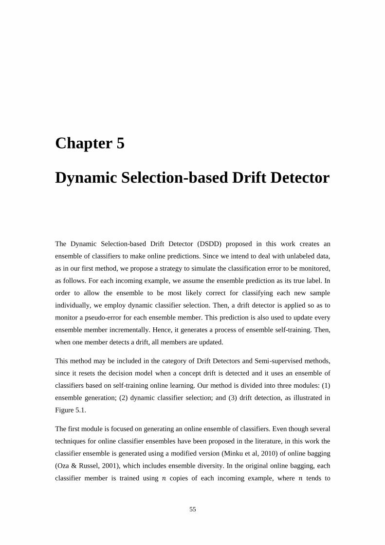
55

Chapter 5

Dynamic Selection-based Drift Detector

The Dynamic Selection-based Drift Detector (DSDD) proposed in this work creates an

ensemble of classifiers to make online predictions. Since we intend to deal with unlabeled data,

as in our first method, we propose a strategy to simulate the classification error to be monitored,

as follows. For each incoming example, we assume the ensemble prediction as its true label. In

order to allow the ensemble to be most likely correct for classifying each new sample

individually, we employ dynamic classifier selection. Then, a drift detector is applied so as to

monitor a pseudo-error for each ensemble member. This prediction is also used to update every

ensemble member incrementally. Hence, it generates a process of ensemble self-training. Then,

when one member detects a drift, all members are updated.

This method may be included in the category of Drift Detectors and Semi-supervised methods,

since it resets the decision model when a concept drift is detected and it uses an ensemble of

classifiers based on self-training online learning. Our method is divided into three modules: (1)

ensemble generation; (2) dynamic classifier selection; and (3) drift detection, as illustrated in

Figure 5.1.

The first module is focused on generating an online ensemble of classifiers. Even though several

techniques for online classifier ensembles have been proposed in the literature, in this work the

classifier ensemble is generated using a modified version (Minku et al, 2010) of online bagging

(Oza & Russel, 2001), which includes ensemble diversity. In the original online bagging, each

classifier member is trained using 𝑛 copies of each incoming example, where 𝑛 tends to

56

𝑃𝑜𝑖𝑠𝑠𝑜𝑛(1) distribution. The modified version includes a parameter λ for the 𝑃𝑜𝑖𝑠𝑠𝑜𝑛(λ)

distribution, where higher/lower λ values lead to lower/higher diversity in the ensemble.

Since our method is online and, in order to detect drifts in unlabeled data, the second module is

intended to select the most competent ensemble member to classify each incoming example.

Thus, for each new (unknown) example 𝑥𝑖, one ensemble member is selected to assign a label

𝑃𝑟𝑒𝑑𝑖 one at a time, such as incoming data in a stream. If a drift is detected, the dynamic

classifier selection module is updated with a new labeled validation dataset. This is the

supervised step of our method.

Finally, the third module is designed to detect drift. Assuming the prediction 𝑃𝑟𝑒𝑑𝑖 provided by

the previous module as the true label, a drift detector is then applied for each ensemble member,

so as to monitor individual pseudo-errors. 𝑃𝑟𝑒𝑑𝑖 is compared to the output provided by each

classifier member. 𝑃𝑟𝑒𝑑𝑖 is also used to update every ensemble member incrementally as a self-

training process. When 𝑡 members detect a drift, all members and the validation dataset are

updated.

The dynamic selection method for the second module and the drift detector for the third module

are parameter to be adjusted in DSDD. In addition, other parameters also need to be set, such as:

ensemble size (𝑇); number of labeled examples to initiate the online bagging (𝑚); number of

members that need to reach the drift level (𝑡); size of initial validation dataset (𝑆); and the

number of nearest neighbors to be used by dynamic selection method (𝑘𝑁𝑁).

The aim of DSDD is to overcome strategies for drift detection based on error monitoring or

system constant update, especially in practical problems whose data are not fully labeled. In this

way, the idea is to detect drift by monitoring pseudo-errors and to update the system only after

drift detection. In order to better describe the overview scheme shown in Figure 5.1, we divided

this chapter into three sections: ensemble creation, selection module, and detection module.

5.1 Ensemble Creation

Motivated by the advantages of classifier ensembles highlighted in the literature concerning data

stream problems, our method is intended to construct diverse ensembles. In addition, the

classifier ensembles must be designed to allow incremental learning.

57

Hence, in the ensemble creation module, we employ a modified version of online bagging

(Minku et al, 2010), summarized in Algorithm 5.1, as follows. The first 𝑚 incoming examples

are manually labeled to start the online bagging training process. For each classifier member,

each training example is presented 𝑛 times, where 𝑛 is defined by 𝑃𝑜𝑖𝑠𝑠𝑜𝑛(𝜆) distribution. It is

important to observe that, as mentioned before, low 𝜆 values lead to high diversity among

ensemble members.

Figure 5.1. Overview scheme of the proposed method (DSDD).

After such a supervised online bagging including the first 𝑚 incoming examples, online bagging

keeps updating the ensemble incrementally, as it is expected. Here, however, the incoming

examples after 𝑚 are no longer manually labeled. The next module (Selection Module) provides

a pseudo true label for every incoming example.

Therefore, online bagging is adapted to work as a self-training method. We have initialized the

online bagging as supervised in order to generate an accurate ensemble and then to be

incrementally updated by self-training.

The base classifiers used in this work are Hoeffding Trees. This choice is especially due to the

fact that bagging is used to improve the performance of unstable algorithms, such as decision

trees (Breiman, 1996).

58

5.2 Selection Module

It was mentioned in Chapter 2 that classifier selection is defined as a strategy that assumes each

ensemble member as an expert in some regions of competence. Thus, rather than combining all

𝑡 classifiers generated by online bagging using a fusion function, dynamic selection chooses a

winning classifier over samples contained in an independent validation dataset, to assign the

label to each 𝑥𝑖 incoming sample.

Algorithm 5.1. Online ensemble creation.

There are several different dynamic classifier selection methods reported in the literature. In this

work, we employ methods based on the assumption that the best-performing classifier over the

local region (k-nearest neighbors) obtained from a validation dataset surrounding 𝑥𝑖 is the most

confident classifier to label it individually. Hence, the second module of our method is designed

to work with a validation dataset, which is created with a small amount of labeled examples.

Two dynamic classifier selection methods are investigated: Dynamic Classifier Selection with

Local Accuracy (DCS-LA) (Woods et al, 1997) and Dynamic Classifier Selection based on

Multiple Classifier Behavior (DS-MCB) (Giacinto & Roli, 2001). These methods follow the

Nearest Neighbor Rule (NN-Rule) (Britto Jr et al, 2014), where methods search for the k-

nearest neighbors (kNN) of 𝑥𝑖 in the validation dataset. Each ensemble member is evaluated

over the kNN of 𝑥𝑖 and the best performing classifier is selected to predict 𝑥𝑖.

𝐾 = 𝐾 − 1;

input: 𝑥: incoming example; 𝑀: ensemble; 𝑇: ensemble size;

begin for 𝑒𝑎𝑐ℎ 𝑥 do

for 𝑗 = 1 𝑡𝑜 𝑇 do 𝐾 = 𝑃𝑜𝑖𝑠𝑠𝑜𝑛(𝜆);

while 𝐾 > 0 do 𝑀𝑗 = 𝐼𝑛𝑐𝑟𝑒𝑚𝑒𝑛𝑡𝑎𝑙𝑈𝑝𝑑𝑎𝑡𝑒(𝑀𝑗; 𝑥);

end end end

59

DCS-LA is a popular accuracy-based method for dynamic classifier selection with two different

versions: Overall Local Accuracy (OLA) and Local Class Accuracy (LCA). The OLA is

computed as the amount of neighbors of 𝑥𝑖 correctly classified by each member classifier 𝑐𝑗.

Then, the member (𝑐∗) with the highest OLA is selected to classify 𝑥𝑖 (Equation 5.1).

𝑐𝑥∗ = 𝑎𝑟𝑔𝑚𝑎𝑥𝑗(𝑂𝐿𝐴𝑗) (5.1)

In the LCA version, for each member classifier 𝑐𝑗, it is computed the number of neighbors of 𝑥𝑖

for which 𝑐𝑗 has correctly assigned class 𝜔, but considering only those examples whose label

(𝜔𝑡) is the same class predicted for 𝑥𝑖 (𝜔𝑥). In this way, the best member classifier for the

current example (𝑐𝑥∗) is the one with the highest LCA (Equation 5.2).

𝑐𝑥∗ = 𝑎𝑟𝑔𝑚𝑎𝑥𝑗(𝐿𝐶𝐴𝑗) | 𝜔𝑡 = 𝜔𝑥 (5.2)

DS-MCB is a behavior-based method that uses a similarity function to measure the degree of

similarity (𝑆𝑖𝑚) of the output of all classifier members. First, for the incoming example 𝑥𝑖 is

computed the vector 𝑀𝐶𝐵𝑥 of class labels assigned by all classifier members. Thus, for each 𝑥𝑖

in the local region (kNN) is also computed the vector 𝑀𝐶𝐵𝑘,𝑡 of class labels assigned by all

classifier members. The method computes the similarity between 𝑀𝐶𝐵𝑥 and each 𝑀𝐶𝐵𝑘,𝑡 to

find a new local region (kNN'), i.e., the examples in kNN with the 𝑀𝐶𝐵 most similar to 𝑀𝐶𝐵𝑥

(Equation 5.3). Finally, kNN' is used to select the most accurate classifier by overall local

accuracy (OLA), such as DCS-LA, to classify 𝑥𝑖.

𝑘𝑁𝑁′ = 𝑘𝑁𝑁′ ∪ 𝑘𝑡 | 𝑆𝑖𝑚(𝑀𝐶𝐵𝑥 , 𝑀𝐶𝐵𝑘,𝑡) > 𝑡ℎ𝑟𝑒𝑠ℎ𝑜𝑙𝑑 (5.3)

Finally, in this module, the prediction (𝑃𝑟𝑒𝑑𝑖) assigned by the selected classifier is assumed as

the true label of 𝑥𝑖 and used in the next module, whatever the dynamic selection strategy used to

select the most confident classifier to label 𝑥𝑖. We may observe these steps in Algorithm 5.2. In

60

the next module, the new validation dataset is collected to replace the current one when a

concept drift occurs.

5.3 Detection Module

In the detection module, we apply a drift detector for each ensemble member. However, since

most of the drift detectors are designed to cope only with labeled data, these methods must be

tailored to support unlabeled data. In order to accomplish this requirement, in our method we

assume that 𝑃𝑟𝑒𝑑𝑖 is the 𝑥𝑖 's true label. Therefore, as in our previous method, our assumption is

that any drift detector based on SPC available in the literature may be used to detect drift in the

unsupervised detection module of our proposed method.

Algorithm 5.2. Selection module algorithm.

In this work, we have tailored two supervised drift detectors to work as unsupervised methods:

DDM and EDDM. It works as follows; a pseudo prequential error rate is monitored for each

classifier member using 𝑃𝑟𝑒𝑑𝑖. For instance, given an ensemble 𝑀 composed of 10 classifiers

𝑀𝑗, where 𝑗 = 1. . .10, there are 10 pseudo prequential error rates to be monitored

simultaneously and individually, i.e. 10 local drift detection processes are conducted. Thus, the

𝑘𝑁𝑁 = 𝑘𝑁𝑒𝑎𝑟𝑒𝑠𝑡𝑁𝑒𝑖𝑔ℎ𝑏𝑜𝑢𝑟𝑠(𝑆; 𝑥);

input: 𝑥: incoming example; 𝑀: ensemble; 𝑇: ensemble size; 𝑆: labeled validation dataset;

output: 𝑒𝑥𝑝𝑒𝑟𝑡: member selected to classify 𝑥; 𝑝𝑠𝑒𝑢𝑑𝑜𝐿𝑎𝑏𝑒𝑙: expert member prediction; begin for 𝑒𝑎𝑐ℎ 𝑥 do

for 𝑗 = 1 𝑡𝑜 𝑇 do 𝑝𝑚𝑐𝑗 = 𝑒𝑣𝑎𝑙𝑢𝑎𝑡𝑒(𝑀𝑗 ; 𝑘𝑁𝑁); //performance of each member

end 𝑒𝑥𝑝𝑒𝑟𝑡 = 𝑠𝑒𝑙𝑒𝑐𝑡𝐶𝑙𝑎𝑠𝑠𝑖𝑓𝑖𝑒𝑟(𝑀; 𝑝𝑚𝑐); //member with best performance 𝑝𝑠𝑒𝑢𝑑𝑜𝐿𝑎𝑏𝑒𝑙 = 𝑝𝑟𝑒𝑑𝑖𝑐𝑡(𝑒𝑥𝑝𝑒𝑟𝑡; 𝑥); //this prediction is assumed as true label

end end

61

set of pairs (𝑃𝑟𝑒𝑑𝑖, 𝑥𝑖) which rely on the local warning level (denoted by 𝑆𝑗) is stored to further

update its respective classifier member.

In terms of DDM, for each member classifier, the warning level and drift level are reached if

conditions (Equation 3.1) or (Equation 3.2) are satisfied, respectively. The 𝑝 value represents

the pseudo error rate of the member classifier, while 𝑠 denotes its standard deviation. The

registers 𝑝𝑚𝑖𝑛 and 𝑠𝑚𝑖𝑛 are set during the training phase, and are updated if after each incoming

example (𝑖) the current register 𝑝𝑖 + 𝑠𝑖 is lower than 𝑝𝑚𝑖𝑛 + 𝑠𝑚𝑖𝑛.

On the other hand, when using EDDM’s SPC, our method calculates the distance (𝑝′) between

two consecutive pseudo errors and their standard deviation (𝑠′), and stores the maximum values

of 𝑝′ and 𝑠′ to register the point where the distance between two errors is maximum (𝑝′𝑚𝑎𝑥 +

2 ∗ 𝑠′𝑚𝑎𝑥). According to Baena et al (2006), the warning level is reached when the Equation 3.3

is lower than α, and the drift level is reached when the same Equation 3.3 is lower than β. These

two thresholds are defined experimentally. In our experiments, we set α=0,95 and β=0,9.

In this detection module, when the first classifier member 𝑀𝑗 reaches its drift level, the whole

system is updated and all parameters (such as prequential error and standard deviation) are reset,

i.e., each classifier member 𝑀𝑗 is updated using its own subset 𝑆𝑗.

However, it is important to mention that only the subset of 𝑀𝑗 is labeled and used as new

validation dataset, in order to reduce the labeling processing time. For the remaining classifiers,

the label of each 𝑥𝑖 contained in each 𝑆𝑗 is assumed to be its respective 𝑃𝑟𝑒𝑑𝑖.

In addition, all members are also updated incrementally based on 𝑃𝑟𝑒𝑑𝑖 due to online bagging

self-training, as discussed previously in this chapter. We can observe all the steps executed by

the detection module in Algorithm 5.3.

In next section, we present experimental results to verify the performance of our proposed

method compared to baselines over several databases. We also compare this method to our

DbDDM method.

5.4 Experiments and Results

A series of experiments has been carried out to evaluate our semi-supervised drift detection

method. Four different versions of combinations of dynamic selection methods and drift

62

detectors are investigated: DCS-LA+DDM, DCS-LA+EDDM, DS-MCB+DDM and DS-

MCB+EDDM. The best version is then compared to SAND, which is a semi-supervised

baseline method described in Chapter 3, and to the supervised baseline DDM. Finally, the

method proposed in this chapter is also compared to our first proposed method DbDDM.

As mentioned before, we have used online bagging as ensemble creation strategy and Hoeffding

Trees as base learning algorithms. The drift detectors were implemented in Matlab 7.10 over

Windows 7 in a machine based on Intel Core i7 3520M@2,90 GHz processor using WEKA

implementations of the learning algorithms. First, however, we will present details related to the

databases investigated in our experiments.

Algorithm 5.3. Detection module algorithm.

In our experiments, we set the following parameters: ensemble size (𝑇) to 10; number of labeled

examples to initiate the online bagging (𝑚) to 30; number of members that need to reach the

drift level (𝑡) to 1; size of initial validation dataset (𝑆) to 30; and the number of nearest

𝑝𝑗 = 1;

𝑟𝑒𝑝𝑙𝑎𝑐𝑒(𝑀𝑗 , 𝑅𝑗);

𝑆𝑗 = 𝑎𝑑𝑑(𝑥);

𝐼𝑛𝑐𝑟𝑒𝑚𝑒𝑛𝑡𝑎𝑙𝑈𝑝𝑑𝑎𝑡𝑒(𝑅𝑗 , 𝑥);

𝑟𝑒𝑠𝑒𝑡(𝑆𝑗);

𝐼𝑛𝑐𝑟𝑒𝑚𝑒𝑛𝑡𝑎𝑙𝑈𝑝𝑑𝑎𝑡𝑒(𝑀𝑗 , 𝑥);

input: 𝑥: incoming example; 𝑀: current ensemble; 𝑅: alternative ensemble; 𝑇: ensemble size; 𝑆: labeled validation dataset;

begin for 𝑒𝑎𝑐ℎ 𝑥 do

for 𝑗 = 1 𝑡𝑜 𝑇 do if 𝑝𝑗𝑟𝑒𝑎𝑐ℎ𝑒𝑠 𝐷𝑟𝑖𝑓𝑡𝐿𝑒𝑣𝑒𝑙 then

𝑙𝑎𝑏𝑒𝑙𝑖𝑛𝑔(𝑆𝑗); //validation dataset for selection module

for 𝑗 = 1 𝑡𝑜 𝑇 do

end break; //go to the next example

end else if 𝑝𝑗𝑟𝑒𝑎𝑐ℎ𝑒𝑠 𝑊𝑎𝑟𝑛𝑖𝑛𝑔𝐿𝑒𝑣𝑒𝑙 then

end else

end end

end

end

63

neighbors to be used by the dynamic selection method (𝑘𝑁𝑁) to 10. The methods selected to

adjust the second and the third modules are described in section 5.4.2.

5.4.1 Databases

Here, we describe the datasets used for the experiments. Some of artificial datasets, such as

SINE1, CIRCLE and SINE1G, are described in Section 4.4.1, previous chapter. Besides SINE1,

CIRCLE and SINE1G, and also investigated LINE, which is described below:

• LINE. Abrupt concept drift, noise-free examples. This dataset presents two relevant

attributes, both assuming values uniformly distributed in [0,1]. The classification

function is given by 𝑦 = −𝑎0 + 𝑎1𝑥1, where 𝑎0 can assume different values to define

different concepts. In this dataset, there are two concepts with high severity.

This artificial dataset has two classes and each class is represented by 50% of the examples, and

each 1000 examples represent a concept. Besides these artificial datasets, we have used real

datasets in our experiments. It is important to mention that, in the context of real data, we do not

know when the drifts occur and which type of drifts occur. The real datasets are described

below:

• ELEC2. According to Gama et al. (2006), this dataset is composed of 45312 instances

dated from 7 May 1996 to 5 December 1998. Each example of the database refers to a

period of 30 minutes and has 5 fields: day of week, time stamp, NSW electricity

demand, Vic electricity demand, the scheduled electricity transfer between states and

the class label. The latter identifies the change of the price related to a moving average

of the last 24 hours.

• LUXEMBOURG. It was constructed using European Social Survey 2002-2007. The

task focus on classifying a subject with respect to the internet usage, whether is high or

low. Each data sample is represented as a 20-dimensional feature vector. These features

were selected as general demographic representation. The dataset is balanced 977 + 924

samples for each class. More details about the dataset creation and data source are

found in (Zliobaite, 2011) and (R. Jowell and the Central Coordinating Team, 2003;

2005; 2007).

• KDDCUP99. This is the dataset used for The Third International Knowledge Discovery

and Data Mining Tools Competition, which was held in conjunction with KDD-99 The

Fifth International Conference on Knowledge Discovery and Data Mining. This dataset

64

contains simulated intrusions in a military network traffic based on data collected

during 7 weeks. KDDCUP99 has approximately 4.900.000 examples, which contain 41

features and are labeled as “bad” (intrusions or attacks) or “good” (normal) connections.

We use for our experiments a set containing 10% of the original dataset examples.

5.4.2 Comparison of Different Versions of the Proposed Method

The purpose of these experiments is to compare the performance of our detection method in

different versions of combinations of dynamic selection methods and drift detectors. The

combinations experimented in this work are: DCS-LA+DDM, DCS-LA+EDDM, DS-

MCB+DDM and DS-MCB+EDDM. These versions are used for experiments in both artificial

and real datasets. All experiments in this work using DCS-LA are based on OLA version.

The aim of this comparison is to select the version of our method considered with the best

performance to be compared to the baselines (DbDDM, SAND and DDM).

5.4.2.1 Experiments on Artificial Datasets

First, we analyze the results obtained on experiments using artificial datasets, which allow

getting true, false and missing detections, as well as average detection delays, since it is well

known the right moment when the drifts occur.

In Figure 5.2, we can observe the prequential error in artificial datasets using the dynamic

selection method DCS-LA combined to DDM (red lines) and EDDM (blue lines). These plots

present datasets containing abrupt drifts, such as SINE1 and LINE, and gradual drifts, such as

CIRCLE and SINE1G.

Both versions using DCS-LA as dynamic selection strategy present results quite similar on

abrupt drift datasets SINE1 and LINE in terms of detecting drifts at the right moment and

keeping low prequential error. For the gradual drift datasets CIRCLE and SINE1G, it is more

difficult to identify a pattern behavior due to the fact that there are drift detections at the right

moment, but detections with long delays and detections before drift are also verified. Even

though, both versions keep low prequential error rates when new concepts appear. In all

65

experiments, delays in the drift detections are verified, but we may point out that DCS-

LA+EDDM detects drifts earlier than DCS-LA+DDM.

Figure 5.2. Prequential error of versions DCS-LA+DDM (red lines) and DCS-LA+EDDM (blue lines) on

artificial datasets. Top Left: SINE1; Top Right: LINE; Bottom Left: CIRCLE; Bottom Right: SINE1G.

Figure 5.3 shows plots presenting the prequential error in artificial datasets obtained when using

the dynamic selection method DS-MCB combined to DDM (red lines) and EDDM (blue lines).

For the abrupt drift datasets (SINE1 and LINE), both versions with DS-MCB detected drift at

the right moment and decreased the prequential error rate. However, DS-MCB+EDDM

outperformed DS-MCB+DDM since it presents a smaller number of false detections on SINE1

and earlier reaction on LINE datasets. For CIRCLE, both versions missed detections. Finally,

for SINE1G dataset, DS-MCB+EDDM did not detect the last drifts.

66

Figure 5.3. Prequential error of versions DS-MCB+DDM (red lines) and DS-MCB+EDDM (blue lines)

on artificial datasets. Top Left: SINE1; Top Right: LINE; Bottom Left: CIRCLE; Bottom Right: SINE1G.

If we compare the two versions with DS-MCB to the versions with DCS-LA, some observations

can be made from these results: (1) the proposed method using DCS-LA combined to both drift

detectors was able to decrease the prequential error rate while learning the new concept before it

ended, even with no access to the whole data labels; (2) the two versions using DS-MCB

detected all the abrupt drifts but failed to detect some gradual drifts. Table 5.1 summarizes the

comparison among all four versions of the proposed method in terms of accuracy, total number

of true detections, false detections and missing detections for each dataset. The items presented

in Table 5.1 are defined as follows:

• Accuracy: the percentage of examples correctly classified in the whole dataset;

• Average detection delay: the average number of examples between drift occurrence

and true drift detection of all concept drifts. In SINE1G, detections during all transition

period are not considered delayed;

• True detections: drift detections at the right moments. For abrupt drifts, we consider

only the first detection after drift occurrence; for gradual drifts, we consider all the

detections occurred in the transition period from one concept to another;

67

• False detections: for abrupt drifts, we consider all the detections after true detection in

the same concept; for gradual drifts, we consider all the detections out of transition

period since any detection have occurred in the transition period, otherwise, we use the

same rule used for abrupt drifts;

• Missing detections: concept drifts which are not detected by the method, i.e. false

negatives.

From this table, it is possible to observe that only versions including DS-MCB present missing

detections on datasets with gradual drifts. This result may be due to the similarity function,

which provides wrong new local regions in the transition period. On the other hand, the two

versions involving DCS-LA are able to detect all drifts in all datasets. In the next section, we

present experimental results to verify whether or not these results are observed considering real

datasets.

Table 5.1. Classification accuracy (acc), average detection delay (delay), total number of true detections

(TD), false detections (FD) and missing detections (MD) of different versions of DSDD in each artificial

dataset.

DSDD version Dataset acc(%) delay TD FD MD

DCS-LA+DDM

SINE1 87,91 27 9 2 0

LINE 94,8 130 1 0 0

CIRCLE 90,33 280 3 1 0

SINE1G 81,13 0 35 2 0

DCS-LA+EDDM

SINE1 85,23 25 9 1 0

LINE 96,4 65 1 0 0

CIRCLE 91,1 287 3 1 0

SINE1G 77,7 0 49 22 0

DS-MCB+DDM

SINE1 74,64 70 9 11 0

LINE 92,6 246 1 0 0

CIRCLE 84,42 32 1 1 2

SINE1G 75,26 0 33 12 0

DS-MCB+EDDM

SINE1 80,14 65 9 4 0

LINE 94,3 161 1 0 0

CIRCLE 75,35 248 1 0 2

SINE1G 63,43 0 36 10 2

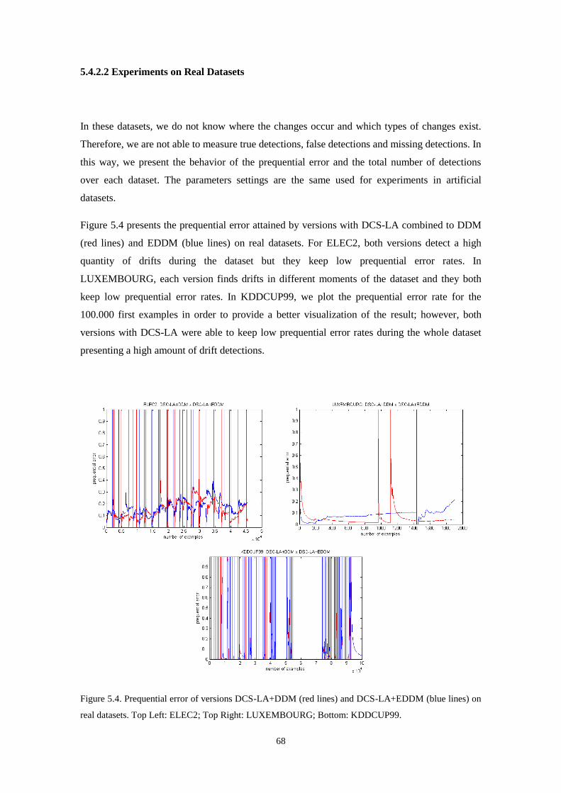
68

5.4.2.2 Experiments on Real Datasets

In these datasets, we do not know where the changes occur and which types of changes exist.

Therefore, we are not able to measure true detections, false detections and missing detections. In

this way, we present the behavior of the prequential error and the total number of detections

over each dataset. The parameters settings are the same used for experiments in artificial

datasets.

Figure 5.4 presents the prequential error attained by versions with DCS-LA combined to DDM

(red lines) and EDDM (blue lines) on real datasets. For ELEC2, both versions detect a high

quantity of drifts during the dataset but they keep low prequential error rates. In

LUXEMBOURG, each version finds drifts in different moments of the dataset and they both

keep low prequential error rates. In KDDCUP99, we plot the prequential error rate for the

100.000 first examples in order to provide a better visualization of the result; however, both

versions with DCS-LA were able to keep low prequential error rates during the whole dataset

presenting a high amount of drift detections.

Figure 5.4. Prequential error of versions DCS-LA+DDM (red lines) and DCS-LA+EDDM (blue lines) on

real datasets. Top Left: ELEC2; Top Right: LUXEMBOURG; Bottom: KDDCUP99.

69

In Figure 5.5, we can observe the prequential error of the versions with DS-MCB combined to

DDM (red lines) and EDDM (blue lines) on real datasets. In ELEC2, the results are quite

similar to the results using DCS-LA: a lot of detections during the dataset and decreasing the

prequential error. In LUXEMBOURG, DS-MCB+DDM was able to decrease the prequential

error rate after first detection, while DS-MCB+EDDM keeps the prequential error stable after

detection. In KDDCUP99, both versions keep low prequential error rates, but it is possible to

observe that DS-MCB+EDDM presents less detections than DS-MCB+DDM, and consequently

lower accuracy rate.

Figure 5.5. Prequential error of versions DS-MCB+DDM (red lines) and DS-MCB+EDDM (blue lines)

on real datasets. Top Left: ELEC2; Top Right: LUXEMBOURG; Bottom: KDDCUP99.

Table 5.2 presents the classification accuracy and total number of detections attained by the four

versions of DSDD at the end of each dataset. The same behavior pointed out for the artificial

datasets was observed for the real databases investigated: versions using DCS-LA outperformed

the DS-MCB-based versions. In terms of accuracy rates, for ELEC2 dataset, DCS-LA+DDM

was slightly superior to DCS-LA+EDDM, while the difference between DCS-LA+DDM and

DS-MCB-based versions was higher. Even though, the performances attained by all four

versions are quite similar, since they present accuracy rates ranging from 81,12% to 84,16%.

70

Table 5.2. Classification accuracy (acc) and total number of detections of different versions of DSDD in

each real dataset.

DSDD version Dataset acc(%) Detections

DCS-LA+DDM

ELEC2 84,16 18

LUXEMBOURG 97,53 2

KDDCUP99 96,28 258

DCS-LA+EDDM

ELEC2 83,03 20

LUXEMBOURG 87,01 1

KDDCUP99 95,13 262

DS-MCB+DDM

ELEC2 81,12 17

LUXEMBOURG 83,75 2

KDDCUP99 95,82 266

DS-MCB+EDDM

ELEC2 81,45 21

LUXEMBOURG 76,12 2

KDDCUP99 90,92 206

Finally, these accuracies show that our DCS-LA+DDM version is able to cope with drifts

presented in LUXEMBOURG and KDDCUP99 datasets classifying correctly more than 90% of

the examples, in despite of using labels partially only. On the other hand, DS-MCB+EDDM

presents the lowest accuracy rates for LUXEMBOURG (76,12%) and KDDCUP99 (90,92%), it

may due to the concepts with small number of examples or to the sensitivity to outliers.

In response to the question posed in the beginning of this section, i.e., which is the best version

of DSDD? DCS-LA+DDM may be deemed to be the best strategy. First, based on the

classification accuracy results, this version attained the highest rate in 5 datasets (2 artificial and

the 3 real datasets) out of a total of 7 datasets investigated. In addition, DCS-LA+DDM does not

present missing detections in none of the artificial datasets. In this way, we choose the version

DCS-LA+DDM to be compared to the baselines in the next section, due to its best performances

in high accuracy rates and true detections.

5.4.3 Comparison of the Proposed Method to Baselines

In these experiments, we intend to compare the best version of DSDD selected by previous

experiments (DCS-LA+DDM) to DbDDM and two different baselines. The first baseline is

SAND, a semi-supervised method such as ours; and the second baseline is the supervised

method DDM. The objective of this comparison is to show that our method is able to deal with

71

concept drifts even when there are no fully labels available. We choose DDM because it is part

of the selected version of DSDD.

It is important to mention that there is no comparison in terms of prequential error due to the

fact that SAND does not provide results in prequential error. Thus, the comparison summarized

in Tables 5.3 and 5.4 is performed by taking into account other measures such as accuracy,

delay, true and false detections, etc.

5.4.3.1 Experiments on Artificial Datasets

For these experiments, we include the number of labeled examples as evaluation metric for the

methods. In addition, Table 5.3 also presents the classification accuracy, average detection

delay, total number of true detections, false detections and missing detections of our method

DCS-LA+DDM, DbDDM, SAND and DDM at the end of each dataset. DCS-LA+DDM was

able to detect all drifts in all datasets such as DDM. In SINE1G dataset, our method presents a

high quantity of true detections in all experiments, but it is important to say that the detections

were suggested in the transition period of 1000 examples. In addition, DCS-LA+DDM reaches

high accuracy rates such as both baselines.

DbDDM presents accuracy rates quite similar to the other methods investigated. Although this

method uses 100% of the labeled examples, the detection module monitors a pseudo-error.

DbDDM detects all drifts at the right moment with no false or missing detections.

The results achieved using DDM were expected, since it is a supervised drift detector. DDM

presented the best performance on attaining the highest accuracy rates, with no false detections

or missing detections. However, in terms of accuracy rates, the rates reached by DCS-

LA+DDM and SAND were on average 6% lower than DDM's accuracy rates for SINE1, LINE

and CIRCLE datasets, while both semi-supervised methods outperformed DDM in SINE1G

dataset. Especially noteworthy is the fact that the semi-supervised methods dealt with only 5%

of labeled data, on average, in order to attain these high accuracy rates.

In terms of number of labeled examples, our method selects those examples that rely on

warning level by statistical tests; while SAND selects those examples based on classifier

confidence lower than a threshold. In this way, SAND presents a more robust method to select

few examples among more recent examples to be labeled. However, in datasets such as SINE1

and SINE1G, SAND presents more missing detections than true detections. Such a weak result

may be due to the classification function of these datasets. Since the classification is reversed

72

after concept drifts, in this case, the classifier confidence will remain high but the predictor will

classify data incorrectly. In addition, SAND is strongly dependent on fine-tuning the threshold

parameter. SAND missed 8 true detections in SINE1 dataset and 7 true detections in SINE1G

dataset. While in LINE and CIRCLE datasets, SAND takes advantage since it presents lower

detection delays.

From this table, some observations can be made:

Our semi-supervised drift detector outperformed the semi-supervised baseline SAND in

all aspects investigated, except for the percentage of labeled examples.

When comparing our two proposed methods, except for LINE dataset, DbDDM

achieved higher accuracy rates. In terms of detection delay, DCS-LA+DDM presents

higher delay, in general. The same scenario is observed when false detection is taken

into account. Therefore, we may conclude that, in practical problems, when the true

labels of newly instances are immediately available, DbDDM is more effective than

DCS-LA+DDM.

Table 5.3. Classification accuracy (acc), average detection delay (delay) number of true detections (TD),

false detections (FD), missing detections (MD) and percentage of labeled examples (lbl) in each dataset.

Method dataset acc(%) delay TD FD MD lbl(%)

DCS-LA+DDM (DSDD)

SINE1 87,91 27 9 2 0 1,6

LINE 94,8 130 1 0 0 0,25

CIRCLE 90,33 280 3 1 0 1,05

SINE1G 81,13 0 35 2 0 0,5

DbDDM

SINE1 91,37 73 9 0 0 100

LINE 93,20 92 1 0 0 100

CIRCLE 92,82 154 3 0 0 100

SINE1G 83,95 0 20 0 0 100

SAND

SINE1 84,25 95 1 0 8 0,03

LINE 94,9 83 1 0 0 0,1

CIRCLE 91,4 15 3 3 0 0,1

SINE1G 83,12 0 3 0 7 0,02

DDM

SINE1 96,28 11 9 0 0 100

LINE 97,55 25 1 0 0 100

CIRCLE 96,8 32 3 0 0 100

SINE1G 79,67 0 13 0 0 100

73

5.4.3.2 Experiments on Real Datasets

As mentioned before, with real datasets we can evaluate the classification accuracy, the total

number of detections and the percentage of labeled examples in the whole dataset. In order to

compare DSDD to DbDDM, SAND and DDM, we choose again the version DCS-LA+DDM

due to the best performance at decreasing prequential error in both real datasets.

In Table 5.4, we can observe that DCS-LA+DDM presents the highest accuracy rate in

LUXEMBOURG dataset followed by DbDDM, and both probably find two true detections.

SAND takes advantage in accuracy on ELEC2 while our method reaches accuracy rates quite

similar to DbDDM and DDM. However, in ELEC2, DCS-LA-DDM presents the smallest

number of detections, which implies in lower computational costs. In addition, our method and

SAND reach high accuracy rates even using a limited number of labeled examples.

In terms of the KDDCUP99 dataset, our method reaches higher accuracy rates than DbDDM

and accuracy rates quite similar to DDM, despite using only 23,01% of labeled examples. In

addition, for this last dataset, SAND reaches the lowest accuracy rates compared to the other

investigated methods.

Table 5.4. Classification accuracy (acc), total number of detections, and percentage of labeled examples

(lbl) in each real dataset.

method Dataset acc(%) detections lbl(%)

DCS-LA+DDM (DSDD)

ELEC2 84,16 18 0,4

LUXEMBOURG 97,53 2 6,0

KDDCUP99 96,28 258 23,01

DbDDM

ELEC2 81,55 78 100

LUXEMBOURG 93,61 2 100

KDDCUP99 90,11 192 100

SAND

ELEC2 94,62 44 0,1

LUXEMBOURG 85,11 1 1,0

KDDCUP99 74,81 190 0,5

DDM

ELEC2 83,06 128 100

LUXEMBOURG 79,80 0 100

KDDCUP99 99,91 53 100

74

It is also important to mention that both semi-supervised methods DCS-LA+DDM and SAND

outperformed DDM on real datasets, except for KDDCUP99, which was not an expected result,

since DDM is a supervised method. These interesting results indicate that semi-supervised

methods, besides reducing the dependence on labeled data, may also deal very

effectively with drifts in real application problems.

5.5 Final Considerations

The DSDD also intends to deal with data streams in practical problems since it detects drifts and

reacts to them considering unlabeled data. Its main goals are to estimate the pseudo error to be

monitored, and to overcome the main DbDDM’s drawback, i.e. supervised reference cluster

update.

To ensure good online predictions to be assumed as “true labels” and to estimate the pseudo

error, we use dynamic classifier selection in a diverse ensemble of classifiers generated by

online bagging. The predicted label is used to update each ensemble member incrementally.

To detect drifts, drift detectors are applied independently and simultaneously for each ensemble

member. They monitor different prequential pseudo error rates until the first member suggests a

drift detection. This is moment when the whole ensemble is updated using recent examples.

This proposed method is flexible enough to be adjusted to different dynamic classifier selection

techniques and different drift detectors. We experimented four different combinations using real

and artificial datasets in order to select the best one to be compared to other baselines. The best

results were attained to the combination DCS-LA+DDM.

Moreover, we compared this DSDD version (DCS-LA+DDM) to three baselines, DbDDM,

SAND and DDM. Our method achieved competitive results in terms of accuracy rates, drift

detection at the right moments and drift reaction delays. In addition, DSDD and SAND were

able to achieve good performances even using a limited amount of labeled data. Finally, the

DSDD outperformed DDM over real datasets, which is an unexpected result since DDM is a

supervised method.

75

Chapter 6

Conclusions

This work proposes two new methods to be applied in practical problems involving data stream,

such as spam filtering and fraud detection. The objective of the proposed methods is to maintain

low error rates, even in the presence of concept drifts, by detecting drifts and adapting the

classification system to the new concepts. The main goals of this work is to avoid strategies that

detect drifts relied on system performance decreasing, i.e. based on error monitoring; and to

avoid blind update-based strategies, which update the system constantly, whatever the drift

detection is implicit or explicit.

The first proposed method, DbDDM, is based on two modules: dissimilarity and detection,

which share the same application, but can be used in collaboration or independently. DbDDM

uses the dissimilarity calculated between current and past data to estimate the pseudo

prequential error. Based on pseudo prequential error values, DbDDM may employ the same

statistical tests conducted in traditional drift detectors to suggest drifts. In this work, DDM and

EDDM were investigated as drift detectors for DbDDM. This proposed method also maintains

the decision model until drift detection, when the system reacts by updating the decision model

(current classifier and reference clusters) using the next examples by one-pass learning, and

consequently, forgetting the previous knowledge. However, even though this method does not

use the true label for drift detection, it deals with clusters which are updated incrementally in a

fully supervised way.

It is important to mention that in practical problems we may not assume that the true labels of

the instances are fully and immediately available after classification, as expected for DbDDM.

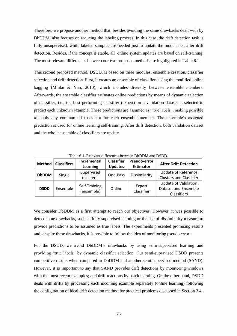
76

Therefore, we propose another method that, besides avoiding the same drawbacks dealt with by

DbDDM, also focuses on reducing the labeling process. In this case, the drift detection task is

fully unsupervised, while labeled samples are needed just to update the model, i.e., after drift

detection. Besides, if the concept is stable, all online system updates are based on self-training.

The most relevant differences between our two proposed methods are highlighted in Table 6.1.

This second proposed method, DSDD, is based on three modules: ensemble creation, classifier

selection and drift detection. First, it creates an ensemble of classifiers using the modified online

bagging (Minku & Yao, 2010), which includes diversity between ensemble members.

Afterwards, the ensemble classifier estimates online predictions by means of dynamic selection

of classifier, i.e., the best performing classifier (expert) on a validation dataset is selected to

predict each unknown example. These predictions are assumed as “true labels”, making possible

to apply any common drift detector for each ensemble member. The ensemble’s assigned

prediction is used for online learning self-training. After drift detection, both validation dataset

and the whole ensemble of classifiers are update.

Table 6.1. Relevant differences between DbDDM and DSDD.

Method Classifiers Incremental

Learning Classifier Updates

Pseudo-error Estimator

After Drift Detection

DbDDM Single Supervised (clusters)

One-Pass Dissimilarity Update of Reference Clusters and Classifier

DSDD Ensemble Self-Training (ensemble)

Online Expert

Classifier

Update of Validation Dataset and Ensemble

Classifiers

We consider DbDDM as a first attempt to reach our objectives. However, it was possible to

detect some drawbacks, such as fully supervised learning or the use of dissimilarity measure to

provide predictions to be assumed as true labels. The experiments presented promising results

and, despite these drawbacks, it is possible to follow the idea of monitoring pseudo error.

For the DSDD, we avoid DbDDM’s drawbacks by using semi-supervised learning and

providing “true labels” by dynamic classifier selection. Our semi-supervised DSDD presents

competitive results when compared to DbDDM and another semi-supervised method (SAND).

However, it is important to say that SAND provides drift detections by monitoring windows

with the most recent examples; and drift reactions by batch learning. On the other hand, DSDD

deals with drifts by processing each incoming example separately (online learning) following

the configuration of ideal drift detection method for practical problems discussed in Section 3.4.

77

In addition, when compared to a supervised method (DDM), DSDD attained performances quite

similar or even better, such as the classification accuracy reached on all investigated real

datasets. These results were not expected since DDM is a supervised drift detector.

6.1 Limitations and Future Work

Given that the second proposed method (DSDD) is accomplished using unlabeled data and

avoiding blind updates, the drift detections, classification error rates and the system reaction

delays attained by our method may be assumed to be very promising, but subjected to more

analysis aiming to decrease the prequential error rates and leading drift reactions to be faster.

This method reacts to drifts by replacing the whole ensemble of classifiers when a concept drift

is detected. This may increase the prequential error rate when recurring concepts are involved.

In addition, it may increases the reaction delay since all classifier members represent the same

concept and all of them need to be replaced after drift detection.

For future work, in the drift reaction system, an alternative to overcome the drawbacks

mentioned before is to remove the poorest performing member classifier when adding a new

member containing examples of the new concept. In this way, it is possible to maintain previous

knowledge and, consequently, reducing prequential error rates and the reaction delay

Moreover, DSDD experiments used dynamic selection methods of a single classifier. The

selection module of DSDD may also be adjusted to use dynamic ensemble selection methods

such as KNORA (k-Nearest-Oracles) proposed by Ko et al (2008); since there is more than one

expert, it may assure better predictions in transition periods between different concepts.

Another issue to investigate is the ensemble generation process. The proposed method creates a

diverse ensemble by online bagging using self-training. Other ensemble generation techniques

(such as mentioned in section 2.3.2.1) may be combined to self-training and adapted to online

systems.

Finally, our proposed method, DSDD, uses semi-supervised learning selecting a small number

of examples to be labeled by applying statistical tests on pseudo error monitoring. There are

others example query strategies (Settles, 2010) that may be investigated to reduce the labeling

process, such as query by ensemble that label those examples for which the ensemble members

disagree the most.

78

References

Adae, I., and Berthold, M. R. EVE: a framework for event detection. In: Evolving Systems;

Volume 4, (2013), Issue 1, 61-70.

Almeida, P. R. L., Oliveira, L. S., Britto Jr, A. S., Sabourin, R.: Handling Concept Drifts Using

Dynamic Selection of Classifiers. In: Proceedings of the IEEE International Conference

on Tools with Artificial Intelligence (ICTAI'16), San Jose, CA, USA, 6-8 November,

2016.

Alpaydin, E. Introduction to Machine Learning. Edition 2, The MIT Press, 2009, 584 p. ISBN:

9780262012430.

Altinçay, H. Ensembling evidential k-nearest neighbor classifiers through multi-modal

perturbation. Appl. Soft Comput. 7 (June 2007), 1072-1083.

Baena-Garcia, M., Del Campo-Ávila, J., Fidalgo, R., Bifet, A. Early drift detection method. In

ECML PKDD 2006 Workshop on Knowledge Discovery from Data Streams (2006), 77-

86.

Bose, R.P.J.C., van der Aalst, W.M.P., Zliobaite, I., Pechenizkiy, M. Dealing With Concept

Drifts in Process Mining. In: Neural Networks and Learning Systems, IEEE Transactions

on (Volume: 25, Issue: 1), 2014, 154-171.

Breiman, L.: Bagging predictors. Machine Learning, v.24, n.2, 123–140, (1996).

Britto Jr, A., Sabourin, R., Oliveira, L. E. S. Dynamic Selection of Classifiers – A

Comprehensive review. Pattern Recognition, Elsevier, 47, (2014), 3665-3680.

79

Brzezinski, D. Mining Data Streams with Concept Drift. Master’s thesis, School: Poznan

University of Technology, Poznan, 2010.

Brzezinski, D., and Stefanowski, J. Reacting to Different Types of Concept Drift: The Accuracy

Updated Ensemble Algorithm. In: Neural Networks and Learning Systems, IEEE

Transactions on (Volume: 25, Issue: 1), 2014, 81-94.

Camps-Valls, G., and Bruzzone, L. Kernel methods for remote sensing data analysis. Wiley

Online Library, 2009.

Chandola, V., Banerjee, A. and Kumar, V. Anomaly Detection: A Survey. ACM Comput. Surv.

41, 3, Article 15, 58 p., 2009.

Chen, H., Ma, S., Jiang, K. Detecting and Adapting do Drifting Concepts. In: Proceedings of

9th International Conference on Fuzzy Systems and Knowledge Discovery, Chongqing,

2012.

Dawid, A. and Vovk, V. Prequential Probability: Principles and Properties, Bernoulli, vol. 5,

no. 1, pp. 125–162, 1999.

Ditzler, G., and Polikar, R. Incremental Learning of Concept Drift from Streaming Imbalanced

Data. In IEEE Transactions On Knowledge And Data Engineering, vol. 25, no. 10, 2013.

Fanizzi, N., Amato, C. and Esposito, F. Conceptual Clustering: Concept Formation, Drift and

Novelty Detection. The Semantic Web: Research and Applications. Lecture Notes in

Computer Science Volume 5021, 2008, 318-332.

Faria E.R., Gonçalves I. J. C. R., de Carvalho A. C. P. L. F., Gama J. Novelty detection in data

streams. Artif Intell Rev 2016, 45:235–269.

Gama, J., and Castillo, G. Learning with local drift detection. In Advanced Data Mining and

Applications, X. Li, O. Zaïane, and Z. Li, Eds., vol. 4093 of Lecture Notes in Computer

Science. Springer Berlin/Heidelberg, 2006, 42-55.

Gama, J., Zliobaite, I., Bifet, A., Pechenizkiy, M, and Bouchachia, A. A Survey on Concept

Drift Adaptation. In Journal ACM Computing Surveys (CSUR), Volume 46, Issue 4,

April 2014, Article No 44.

Giacinto, G., Roli, F. Dynamic Classifier Selection based on Multiple Classifier Behavior,

Pattern Recognition. 34, 2001, 1879–1881.

80

Gomes, J.B., Gaber, M.M., Sousa, P.A.C., Menasalvas, E. Mining Recurring Concepts in a

Dynamic Feature Space. In: Neural Networks and Learning Systems, IEEE Transactions

on (Volume: 25, Issue: 1), 2014, pp. 95- 110.

Haque, A., Khan, L., Baron, M. SAND: Semi-Supervised Adaptive Novel Class Detection and

Classification over Data Stream. In Thirtieth AAAI Conference on Artificial Intelligence,

Phoenix, Arizona, USA, 2016.

Harries, M.B., Sammut, C., Horn, K. Extracting hidden context. Machine Learning, 32(2):101-

126, 1998.

Hee Ang, H., Gopalkrishnan, V., Zliobaite, I., Pechenizkiy, M., Hoi, S.C.H. Predictive

Handling of Asynchronous Concept Drifts in Distributed Environments. IEEE

Transactions on Knowledge and Data Engineering, vol. 25, no. 10, pp. 2343-2355, Oct.

2013, doi:10.1109/TKDE.2012.172

Ho, T. K. The random subspace method for constructing decision forests. IEEE Transactions on

Pattern Analysis and Machine Intelligence, v. 20, n. 8, p. 832-844, 1998.

Johansson, U., Lofstrom, T., Niklasson, L. The importance of diversity in neural network

ensembles - an empirical investigation. International Joint Conference on Neural

Networks, pp 661-666, 2007.

Kantardzic, M., Ryu, J.W., Walgampaya. C. Building a New Classifier in an Ensemble Using

Streaming Unlabeled Data. In Proceedings of 23rd International Conference on Industrial

Engineering and Other Applications of Applied Intelligent Systems, IEA/AIE 2010,

Cordoba, Spain, 77-86, (2010).

Karnick, M., Ahiskali, M., Muhlbaier, M., Polikar, R. Learning concept drift in nonstationary

environments using an ensemble of classifiers based approach. In Neural Networks,

2008. IJCNN 2008. (IEEE World Congress on Computational Intelligence). IEEE

International Joint Conference on, 2008, pp. 3455-3462.

Katakis, I., Tsoumakas G., Vlahavas I. Tracking recurring contexts using ensemble classifiers:

an application to email filtering. Knowledge and Information Systems 22, 2010, pp. 371-

391.

Katakis, I., Tsoumakas, G., Vlahavas I. Dynamic feature space and incremental feature

selection for the classification of textual data streams. In: ECML/PKDD-2006

international workshop on knowledge discovery from data stream, 2006, pp 107–116.

81

Kittler, J., Hatef, M., Duin, R. P. W. and Matas, J. On Combining Classifiers. IEEE

Transactions on Pattern Analysis and Machine Intelligence, vol 20, no.3, March, 1998,

226-239.

Kmieciak, M., and Stefanowski, J. Handling Sudden Concept Drift in Enron Messages Data

Stream. draft version of a paper finally published in T. Morzy, M.Gorawski, R.Wrembel,

A.Zgrzywa (ed.) Technologie przetwarzania danych. Mat. III KNTPD Conf., Poznan 21-

23 April 2010, WNT Press, 2010, 284-296.

Ko, A. H. R., Sabourin, R. and Britto Jr. A. S. From Dynamic Classifier Selection to Dynamic

Ensemble Selection, Pattern Recognition.41(5), (2008), pp.1718–1731.

Kolter, J.Z. and Maloof, M.A. Dynamic Weighted Majority: An Ensemble Method for Drifting

Concepts. J. Machine Learning Research, vol. 8, pp. 2755-2790, 2007.

Kuncheva, L. I. Clustering-and-Selection Model for Classifier Combination. In Proceedings of

Fourth International Conference on Knowledge-Based Intelligent Engineering Systems

and Allied Technologies, Volume 1, 2000.

Kuncheva, L. I., Skurichina, M., Duin, R.P.W. An experimental study on diversity for bagging

and boosting with linear classifiers. Information Fusion, v.3, n.4, 245258, 2002.

Kuncheva, L.I. and Whitaker, C.J. Measures of Diversity in Classifier Ensembles and Their

Relationship with the Ensemble Accuracy. Machine Learning, vol. 51, pp. 181-207, 2003.

Kuncheva, L.I. Classifier ensembles for Changing Environments. In Multiple Classifier

Systems, vol. 3077 of Lecture Notes in Computer Science. 2004, pp. 1-157.

Kuncheva, L.I. Classifier ensembles for detecting concept change in streaming data: Overview

and perspectives. In 2nd Workshop SUEMA 2008 (ECAI 2008), pp. 5-10.

Le, T., Tran, D., Nguyen, P., Ma, W., Sharma, D. Multiple Distribution Data Description

Learning Method for Novelty Detection. In: Proceedings of International Joint Conference

on Neural Networks, San Jose, California, USA, 2011.

Markou, M., and Singh, S. Novelty detection: a review. Part 1: statistical approaches. Signal

Processing, 83(12):2481-2497, 2003.

Marsland, S. Novelty detection in learning systems. Neural Computing Surveys, 3:157-195,

2003.

82

Miljkovic, D. Review of Novelty Detection Methods. In Proceedings of MIPRO, Opatija,

Croatia, 2010.

Minku, L., White, A., Yao, X. The Impact of Diversity on On-Line Ensemble Learning in the

Presence of Concept Drift, In IEEE Trans. Knowledge and Data Eng., vol. 22, no. 5,

2010, pp. 730-742.

Minku, L. and Yao, X. DDD: A New Ensemble Approach for Dealing with Concept Drift. In

IEEE Transactions On Knowledge And Data Engineering, Vol. 24, No. 4, April 2012.

Mitchell, T. Machine Learning. McGraw Hill, 1997.

Morsier, F., Borgeaud, M., Kuchler, C., Gass, V., Thiran J. Semi-Supervised And Unsupervised

Novelty Detection Using Nested Support Vector Machines. In: In proceeding of: IEEE

International Geoscience and Remote Sensing Symposium (IGARSS), Munich, 2012

Muhlbaier, M. D., Polikar, R. An Ensemble Approach for Incremental Learning in

Nonstationary Environments. 7th Int. Workshop on Multiple Classifier Systems, in

Lecture Notes in Computer Science, vol 4472, Berlin: Springer, 2007, pp. 490-500.

Muhlbaier, M., Topalis, A., Polikar, R. Learn++.nc: Combining ensemble of classifiers with

dynamically weighted consult-and vote for efficient incremental learning of new classes.

In IEEE Transactions on Neural Networks, vol. 20. 2009, pp. 152-168.

Muñoz-Marí, J., Bovolo, F., Gómez-Chova, Bruzzone, L., Camp-Valls, G. Semisupervised one-

class support vector machines for classification of remote sensing data. IEEE Trans.

Geosci. Remote Sens., vol. 48, no. 8, 2010, pp. 3188 –3197.

Nishida, K., and Yamauchi, K. Detecting concept drift using statistical testing. In Discovery

Science, V. Corruble, M. Takeda, and E. Suzuki, Eds., vol. 4755 of Lecture Notes in

Computer Science. Springer Berlin / Heidelberg, 2007, pp. 264-269.

Oza, N.C. and Russell, S. Experimental Comparisons of Online and Batch Versions of Bagging

and Boosting. Proc. ACM SIGKDD Int’l Conf. Knowledge Discovery and Data Mining,

2001, 359-364.

Otey, M. and Parthasarathy, S. A Dissimilarity Measure for Comparing Subsets of Data:

Application to Multivariate Time Series. In Proceedings of the ICDM Workshop on

Temporal Data Mining, 2005.

Parikh, D.P.R. An ensemble-based incremental learning approach to data fusion. Systems,

Man, and Cybernetics-PartB, IEEE Transactions on 37, 2 (2007), 500-508.

83

Pinagé, F. A. and Santos, E. M. dos. A Dissimilarity-based Drift Detection Method. In:

Proceedings of the IEEE International Conference on Tools with Artificial Intelligence

(ICTAI’15), Vietri Sul Mare, Italy, 9-11 November (2015).

Pinagé, F. A., Santos, E. M. dos, Gama, J. M. P. Classification Systems in Dynamic

Environments: An Overview. WIRES Data Mining and Knowledge Discovery, Published

online: July 15, 2016.

R. Jowell and the Central Coordinating Team. European Social Survey 2002/2003; 2004/2005;

2006/2007. Technical Reports, London: Centre for Comparative Social Surveys, City

University, (2003; 2005; 2007).

Rodríguez, J., and Kuncheva, L. Combining online classification approaches for changing

environments. In Structural, Syntactic, and Statistical Pattern Recognition, N. da Vitoria

Lobo, T. Kasparis, F. Roli, J. Kwok, M. Georgiopoulos, G. Anagnostopoulos, and M.

Loog, Eds., vol. 5342 of Lecture Notes in Computer Science. Springer Berlin /

Heidelberg, 2008, 520-529.

Ruta, D., and Gabrys, B. Classifier Selection for Majority Voting. Information Fusion 6, 1

January 2005, 63-81.

Ruta, D., and Gabrys, B. Neural network ensembles for time series prediction. In Proceedings of

the International Joint Conference on Neural Networks (IJCNN'2007), IEEE Press, 2007,

1204-1209.

Settles, B. Active Learning Literature Survey, Computer Sciences Technical Report 1648.

University of Wisconsin–Madison, 2010.

Sidhu, P., Bhatia, M., Bindal, A. A Novel Online Ensemble Approach for Concept Drift in Data

Streams. In: Proceedings of IEEE Second International Conference on Image Information

Processing (ICIIP), Shimla, 2013.

Smits, P. C. Multiple classifier systems for supervised remote sensing image classification

based on dynamic classifier selection. IEEE Transactions on Geoscience and Remote

Sensing, vol 40, no. 4, 2002, 801-813.

Street, W.N. and Kim, Y. A Streaming Ensemble Algorithm (SEA) for Large-Scale

Classification. Proc. Int’l Conf. Knowledge Discovery and Data Mining, 2001, 377-382.

Tremblay, G., Sabourin, R., Maupin, P. Optimizing nearest neighbor in random subspaces

using a multi-objective genetic algorithm. In Proceedings of the Pattern Recognition, 17th

84

International Conference on (ICPR'04) Volume 1 - Volume 01 (Washington, DC, USA,

2004), ICPR '04, IEEE Computer Society, pp. 208.

Tsymbal, A., Pechenizkiy, M., Cunningham, P., Puuronen, S. Dynamic integration of classifiers

for handling concept drift. Information Fusion. 2008;9(1):56–68.

Valentini, G. Ensemble methods based on bias-variance analysis. PhD thesis, Genova

University, 2003.

Widmer G. and Kubat, M. Learning in the presence of concept drift and hidden contexts. In

Machine Learning, 23:69-101, 1996.

Widmer, G. Combining Robustness and Flexibility in Learning Drifting Concepts. Proceedings

of the 11th European Conference on Artificial Intelligence (pp. 468-472). Chichester:

Wiley & Sons, 1994.

Woods, K., Jr., Kegelmeyer, W. P., Bowyer, K. Combination of multiple classifiers using local

accuracy estimates. IEEE Transactions on Pattern Analysis and Machine Intelligence 19,

1997, 405-410.

Wu, X., Li, P., Hu, X. Learning from concept drifting data streams with unlabeled data.

Neurocomputing, Volume 92, 1 September 2012, 145-155, (2012).

Yule, G. On the Association of Attributes in Statistics. Philosophical Trans. Royal Soc. of

London, Series A, vol. 194, pp. 257-319, 1900.

Zhang, P., Zhu, X., Shi, Y. Categorizing and mining concept drifting data streams. In

Proceeding of the 14th ACM SIGKDD international conference on Knowledge discovery

and data mining (New York, NY, USA, 2008), KDD '08, ACM, pp. 812-820.

Zhu, X., Wu, X., Yang, Y. Dynamic classifier selection for effective mining from noisy data

streams. In Proceedings of the Fourth IEEE International Conference on Data Mining

(Washington, DC, USA, 2004), ICDM '04, IEEE Computer Society, pp. 305_312.

Zliobaite, I. Combining similarity in time and space for training set formation under concept

drift. Intelligent Data Analysis 15(4), 589-611, (2011).

handling concept drift based on data similarity and

Documents