handbook of atmospheric science || synoptic-scale meteorology
TRANSCRIPT
11.1 INTRODUCTION
The adjective “synoptic” literally means the con-sideration of simultaneous observations: in con-sidering weather patterns, which vary in threephysical dimensions and time, it was the develop-ment of synoptic charts in the nineteenth centurythat led to systematic and scientific study of mete-orology, alongside considerable improvements inforecasting skill. The standard observations (“syn-ops”) that go into the production of “synopticcharts” are obtained from “synoptic stations” atthe “synoptic hours” of 0000, 0600, 1200, and 1800UTC. The typical spatial coverage of these stationsmeans that they are well suited to study systemson scales of several hundred kilometers and up-wards, with temporal scales on the order of days:for this reason, the term “synoptic,” which liter-ally means “simultaneous,” has been transposedinto a specification of horizontal scales of a fewhundred to several thousand kilometers. In themid-latitudes this corresponds to the scales offrontal cyclones and blocking highs, for example.In point of completeness, however, it should not beforgotten that the strict definition of the term“synoptic” allows us to discuss global synoptic analyses as well as meso- or microscale synopticanalysis—of an urban region, for instance.
The origins of synoptic analysis being in thestudy of instantaneous datasets, this kind of analy-sis is centered on diagnostics derived from the syn-optic fields. For example, a key aspect of synopticanalysis is to diagnose areas of vertical motion, a
field that is not directly measured, from the fields of horizontal wind and temperature. Thestandard models used for such analysis are based on balanced theories, in which the wind and temperature are assumed to be close to a state in which rotational and pressure gradientforces are in balance. In times when numericalweather prediction far outperforms human fore-casters, such diagnostic methods are the ways inwhich we can interpret complicated numericallycomputed analyses, and even modify numericalforecasts to forecasting advantage. This chapterdescribes such models and the way they are appliedin real contexts.
11.2 BASIC PHYSICALDESCRIPTIONS AND MODELS
This section deals with an overview of the bal-anced models that govern synoptic meteorology.Various textbooks (Carlson 1991; Holton 1992)give detailed derivations of the basic equation sets,and here they are introduced only briefly. In par-ticular, much of the following discussion is concerned with the “dry” evolution of synopticsystems.
11.2.1 Statics, stability, and parcel methods
To a good approximation the air is an ideal gas,with its temperature, T, pressure, p, and density, r,related by
11 Synoptic-Scale Meteorology
DOUGLAS J. PARKER
Handbook of Atmospheric Science: Principles and ApplicationsEdited by C.N. Hewitt, Andrea V. Jackson
Copyright © 2003 by Blackwell Publishing Ltd

276 douglas j . parker
(11.1)
in which R is the gas constant (R = 287Jkg-1 K-1)for dry air. When the air contains water vapor theideal gas law may be expressed as
(11.2)
where r is the mixing ratio, defined as the mass ofwater vapor per unit mass of dry air, and e = R/Rv =0.622 is the ratio of gas constants for dry air andwater vapor. In practice this is accommodated byusing the virtual temperature
(11.3)
Tv is the quantity that may be related to densityand thereby buoyancy in the equations of motionfor the air. Since r is a positive definite quantity and0 < e < 1, air with a higher moisture content is lessdense and has a higher value of Tv. At higher tem-peratures, in the tropical boundary layer, for exam-ple, where the saturation mixing ratio can be 4% orhigher, Tv may differ from T by several Kelvin in moist air. However, at cooler mid-latitude andupper air temperatures, the difference between Tvand T is usually small, so in the coming discussionT will be used.
To a good approximation on synoptic scales, theatmosphere is hydrostatic. This is to say that the pressure distribution in the air is dominated bythe weight of the air column above any given level,and that the dynamic pressure associated with the acceleration of air parcels is insignificant onthese scales. Formally this leads to the hydrostaticrelation:
(11.4)
There are some immediate and important conse-quences of this relation:1 Since density is a positive definite quantity thepressure always decreases upwards under hydro-static conditions. It is this property that makes
∂∂
= -pz
gr
T Trrv =
++
ÊË
ˆ¯
11
e
p RT
rr
=++
ÊË
ˆ¯r
e11
p RT= r pressure a useful surrogate for physical height (forexample, in altimeters). Since pressure decreasesmonotonically with height, synoptic meteorologyis often described in “pressure coordinates” —forexample, (x, y, p) replacing the Cartesian (x, y, z) forflow in rectangular geometry, or (c, l, p) replacingthe spherical polars (c, l, z). Using pressure as aheight scale means that we have a coordinatewhich is also a state variable for the air.2 Integrating the hydrostatic relation from a givenlevel upwards shows that the pressure at any levelin a hydrostatic atmosphere corresponds to theweight of the column of air above that level, perunit area.3 We can deduce an approximate scale height forthe rate of decrease of pressure with height: if it is taken that T variations are small and T may betreated as a constant, eqn 11.4 can be integratedover height (using the ideal gas law) to give
(11.5)
where p0 is the pressure at z = 0, implying a scaleheight zs of
(11.6)
Since pressure corresponds to the weight of the aircolumn, this shows that the bulk of the atmos-phere’s mass lies in the troposphere.4 The hydrostatic relation also leads directly to auseful relation describing the thickness, z1 - z0, ofthe air column between two pressure levels, p0 andp1. Integrating eqn 11.4, using the ideal gas law toeliminate density, the thickness is be found to be
(11.7)
in which is a mean temperature of the layer. Thethickness is an extremely useful quantity in relat-ing mean-state pressure and temperature anom-alies. The 1000–500hPa thickness is often plottedon surface charts, as an aid to estimating meantemperature of the lower troposphere. For forecast-
T
z zRTg
pp1 0
0
1- = ln
zRTgs = ª ¥8 103 m
p p
gzRT
= -ÏÌÓ
¸˝̨0 exp
Synoptic-Scale Meteorology 277
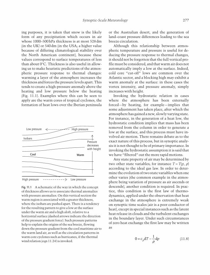
ing purposes, it is taken that snow is the likelyform of any precipitation which occurs in airwhose 1000–500hPa thickness is at most 528dm(in the UK) or 540dm (in the USA; a higher valuebecause of differing climatological stability overthe North American continent), because these values correspond to surface temperatures of lessthan about 0°C. Thickness is also useful in allow-ing us to make heuristic predictions of the atmos-pheric pressure response to thermal changes:warming a layer of the atmosphere increases thethickness and forces the pressure levels apart. Thistends to create a high-pressure anomaly above theheating and low pressure below the heating (Fig. 11.1). Examples where this can be seen toapply are the warm cores of tropical cyclones, theformation of heat lows over the Iberian peninsula
or the Australian desert, and the generation ofland–coast pressure differences leading to the seabreeze circulation.
Although this relationship between atmos-pheric temperature and pressure is useful for de-ducing the pressure response to thermal changes,it should not be forgotten that the full vertical pro-file must be considered, and that warm air does notautomatically imply a low at the surface. Indeed,cold core “cut-off” lows are common over the Atlantic sector, and a blocking high may exhibit awarm anomaly at the surface: in these cases thevortex intensity, and pressure anomaly, simply increases with height.
Invoking the hydrostatic relation in caseswhere the atmosphere has been externallyforced —by heating, for example —implies thatsome adjustment has taken place, after which theatmosphere has gained a new, slowly varying state.For instance, in the generation of a heat low, thehydrostatic condition implies that mass has beenremoved from the column in order to generate alow at the surface, and this process must have in-volved air motion. There remains debate as to theexact nature of this process, but in synoptic analy-sis it is not thought to be of primary importance. Ininvoking the hydrostatic assumption it is said thatwe have “filtered” out the more rapid motions.
Any state property of air may be determined bytwo other state variables; for instance T = T(p, r)according to the ideal gas law. In order to deter-mine the evolution of two state variables when oneother varies (the common example in the atmos-phere being variation of pressure as air ascends ordescends), another condition is required. In prac-tice, this condition is the first law of thermo-dynamics, applied under the observation that heatexchange in the atmosphere is extremely weak on synoptic time scales (air is a poor conductor ofheat), except in special instances such as the latentheat release in clouds and the turbulent exchangesin the boundary layer. Under such circumstancesof zero heat exchange the first law may be writtenas
(11.8)01
= -c T ppd dr
Low pressure High pressure
Pressuredecreaseswith height
WarmCool
Low pressureHigh pressure
Isobars
Fig. 11.1 A schematic of the way in which the conceptof thickness allows us to associate thermal anomalieswith pressure anomalies. On this vertical section thewarm region is associated with a greater thickness,where the isobars are pushed apart. There is a tendencyfor the resulting pattern to give a low at the surfaceunder the warm air and a high aloft, relative to ahorizontal surface (dashed arrows indicate the directionof the pressure gradient force). Such pressure patternshelp to explain the origins of the sea breeze, flowingdown the pressure gradient from the cool maritime air tothe warm land air, as well as the circulation patterns inwarm core cyclones such as hurricanes, if the thermalwind relation (eqn 11.24) is invoked.
278 douglas j . parker
where cp is the specific heat capacity at constantpressure, from which we integrate to obtain
(11.9)
(where for dry air R/cp = 2/7). This is to say that forany given parcel of air, the temperature and pres-sure are related by eqn 11.9, with q a constant forthat parcel. We can rearrange this and label eachparcel of air according to its value of q : q may varyin space, but if the air is disturbed materially, eachparcel carries its q value with it. q is the potentialtemperature of the air and is conserved in adiab-atic motion (for which Q = 0). q is useful not onlybecause it allows us to compute the thermody-namic properties of air as it moves between pressure levels, but also because it allows us tocompare air parcels. Returning to eqn 11.9, it canbe seen that on a given pressure level, air of highertemperature also has higher q : since temperatureis inversely proportional to density on this pres-sure level (from the ideal gas law), q differences re-late directly to density differences on a pressurelevel. It is the density differences that providebuoyancy and determine the principal drivingforces of atmospheric flow. If the basic state q pro-file increases with height, air that is lifted to a level of lower pressure will find itself surrounded by air with a higher potential temperature: the dis-placed air will be cooler and denser than its sur-roundings and tend to sink, and the atmosphere isstable. If the q profile decreases with height, up-wardly displaced air parcels are warmer and lessdense than their environment, and continue torise. These simple arguments lead to the conclu-sion that the static stability of an air profile de-pends on the sign of ∂q/∂z:
∂q/∂z > 0: stable∂q/∂z = 0: neutral∂q/∂z < 0: unstable
Each of these conditions occurs in the atmosphereand characterizes particular flows: for example,unstable conditions generally occur in a boundarylayer that is being forced by solar heating at theground, and correspond to well developed turbu-
T
pp
Rcp=
ÊËÁ
ˆ¯̃
q0
lent convection. High stability is characteristic ofthe stratosphere, frontal zones, and a stable “inver-sion,” capping the boundary layer. A commonmeasure of static stability is the Brunt–Väisälä fre-quency, N, defined by
(11.10)
where q0 is a constant reference value. N repre-sents a characteristic frequency of oscillations ofdisplaced air parcels in an atmosphere that is sta-ble. Typically, in the troposphere, N has a value ofaround 10-2 s-1.
When moist effects are introduced, the ques-tion of stability becomes more complex. However,despite the increased complexity, the differentpossibilities for stability of a given profile can berelated usefully to different cloud and weatherphenomena, so it is worth giving some thought to this topic (a very detailed discussion of moist atmospheric thermodynamics and stability isgiven in Emanuel 1994).
When unsaturated air is lifted adiabatically tolower pressures, its dew point temperature fallsless rapidly than its temperature, so that at somealtitude, known as the lifting condensation level(LCL), these values become equal and the air be-comes saturated. For saturated air, the state vari-ables are linked by the conditions for saturation:the condition that the air remains saturated as itrises beyond the LCL determines the evolution oftemperature and pressure for a given air parcel.This is to say that just as the condition of adiabaticmotion for unsaturated air determines a relation-ship between T and p for a given air parcel, the condition of saturated motion determines anequivalent relationship for saturated parcels, byfixing the water vapor content to a known functionof temperature and pressure. In this way it is possi-ble to construct (given one or two approximations)“equivalent potential temperature,” qe, with thefollowing properties:• qe is conserved in both saturated and unsatur-ated motion;• qe is a function of (T, p) in saturated air, and increases monotonically with T.
Ng
z2
0=

Synoptic-Scale Meteorology 279
There are different assumptions that may be madewhen evaluating qe, regarding the treatment of thedifferent phases of water (for instance, it may be assumed that all condensed water is rained out instantly and no longer contributes to the air parcel thermodynamics). Accurate empirical for-mulae for calculating pseudoadiabatic qe havebeen derived by Bolton (1980):
(11.11)
where p is in hPa and the temperature at the con-densation level can be obtained from
(11.12)
in which e is the vapor pressure in hPa.Note that qe is homeomorphic to the “wet-bulb
potential temperature,” qw, and for the purposes of understanding, the two are interchangeable(though the exact functional values differ). Lines ofconstant qe are also lines of constant qw and theyare termed pseudoadiabats. Note also that although qe is an exact thermodynamic variable in saturated flow, meaning that it is a function ofexactly two other variables such as (p, T), and canbe linked directly to buoyancy, in unsaturated air a third quantity, the air’s moisture content,must be known in order to infer buoyancy from qeand pressure, say. For example, two unsaturatedparcels of air, of the same pressure and tempera-ture, may have differing water vapor contents, andthereby have different values of qe (implying thatone reaches saturation more rapidly than theother). This means that although qe is an attrac-tive variable in that it is universally conserved (under some reasonable approximations), themoisture content of the air must generally still becarried as a variable in order to determine atmos-pheric evolution.
When unsaturated air is lifted, it cools adiabati-cally, from eqn 11.9. When saturated air is lifted, it
TT eL =
- -+
28403 5 4 805
55. ln ln .
qe
r
L
Tp
Tr r
= ÊËÁ
ˆ¯̃
¥ -ÊËÁ
ˆ¯̃
¥ +( )È
ÎÍ
˘
˚˙
- ¥( )1000
33762 54 1 0 81
0 2854 1 0 28. .
exp . .
gains energy from the latent heat release of con-densation, so that it cools at a slower rate than anunsaturated air parcel. Seen another way, the un-saturated air parcel conserves q but the saturatedair experiences an increase in q due to the latentheat release as it rises. This means that an air pro-file which is stable to dry ascent may be unstable tomoist ascent. Making the initial assumption of drystability, there are two principal possibilities, depending on the state of subsaturation of the airprofile, and there is some common confusion in defining the conditions for stability; they aresummarized here:
First, the qe profile of the air determines the con-vective stability of the air (sometimes termed “potential instability”). This means that if the airbecomes saturated, parcels will move along lines ofconstantqe, and arguments entirely analogous to theones determining unsaturated static stability deter-mine moist convective stability criteria dependingon ∂qe/∂z. This condition relates to the stability of alayer of the atmosphere: if it is lifted and cooled tosaturation, how will small perturbations behave inthe saturated layer? Convective instability is mani-fest in cloud forms such as altocumulus, where alayer of ascending air becomes saturated and thenevolves into convective cells.
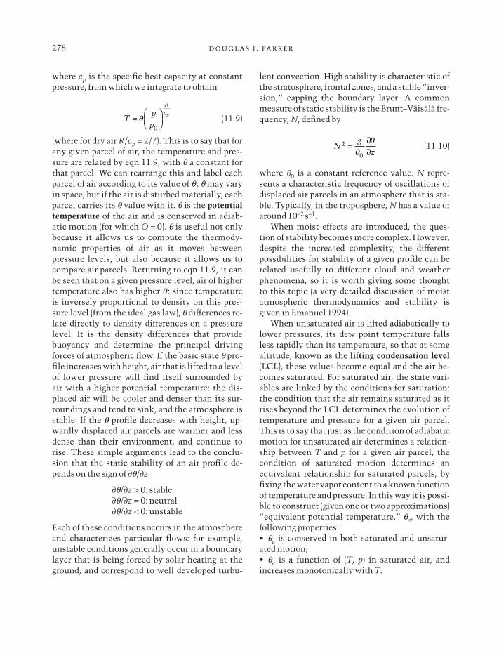
Second, in many instances it is more useful toconsider the stability according to the ascent of an isolated parcel of air over a significant verti-cal distance. In this case, the parcel reaches its lifting condensation level and subsequently rises along a pseudoadiabatic trajectory (conserv-ing qe). At some stage, the parcel may then crossthe environmental profile and become positivelybuoyant (region “PA” in Fig. 11.2). In this instancethe air profile is “conditionally unstable,” mean-ing that small perturbations are stable but signifi-cant displacements of a parcel may lead to freeconvection.
Conditional stability can be inferred from theslope of the environmental sounding with respectto dry and moist (pseudo-) adiabats on a thermody-namic diagram. If the sounding lies between theadiabats and pseudoadiabats, then the air is stableto unsaturated motion but there is a possibility ofsaturated parcels of air following a pseudoadiabat
280 douglas j . parker
that crosses the sounding, leading to conditionalinstability. In practice, conditional instability occurs when there is a relatively cool mid-to-lowertroposphere and a moist, humid surface layer:these conditions will tend to imply convective in-stability also. However, conditional instabilitydoes not depend on the moisture content of the airabove the initial level of the air parcel: just the qe ofthe ascending parcel.
Conditional instability is characteristic of deepcumulus and cumulonimbus clouds. Usually, ad-vection of cool air over a warm and moist boundary
layer sets up this kind of profile, and various triggering mechanisms act to lift air from the surface until it becomes unstable and rises rapidly,gaining potential energy as a result of its buoyancy.Adiabatic descent in response to the cloud acts to reduce the instability by warming the mid-troposphere, as do precipitation-driven down-draughts, which cool the boundary layer.
There are a number of measures of conditionalinstability that are used for forecasting. The Con-vective Available Potential Energy (CAPE) is ameasure of the energy available to a lifted parcel ofair rising from a given level up to cloud top, and iscomputed as
(11.13)
where Tp denotes the temperature of the rising par-cel of air and Tenv is the temperature of the environ-ment. The integral is taken from the initial parcelpressure, pi, up to the level of neutral buoyancy, pn,at which the buoyant, rising parcel returns to theenvironmental profile (Fig. 11.2). Note that theCAPE is a function of the initial choice of ascend-ing air parcel, a choice that influences pi, pn, andTp(p), but does not influence Tenv. Higher values ofCAPE indicate a likelihood of more intense con-vection. Other, simpler diagnostics of conditionalinstability exist: typically they may employ ameasure of the difference between qe (or a surro-gate, such as dew point depression) at two levels,chosen to represent the lower and middle tropo-sphere, in order to estimate the buoyancy of liftedparcels.
Air profiles, as obtained from radiosonde as-cents or from model fields, are generally plotted onthermodynamic diagrams of some kind, for whichthe axes of the diagram are state variables and, forobvious convenience, one of the axes is a functionof p, so that height is upwards on the diagram.While the specifics of such diagrams differ accord-ing to convention and purpose, the generalities arethe same:1 Data are plotted as curves of (T, p) (solid line, byconvention) and (Td, p) (dashed line), where Td isthe dew point.
CAPE R T T d pp envp
p
i
n= - -( )Ú ln
LNB
Environment
PA
Parcel
LFC
NALCL
20 30 40 50 601000
100
Pre
ssure
(hPa)
Potential temperature (°C)
Fig. 11.2 A simple profile of air that is conditionallyunstable (the “Environment” curve). A parcel of air thatis lifted from the surface is initially cooler than itssurroundings but, following condensation (at the liftingcondensation level, LCL), ascends along a pseudoadiabatand can become buoyant (at the level of free convection,LFC). This kind of behavior leads to cumulus andcumulonimbus convection. The parcel finally regainsthe environmental curve and loses its buoyancy at thelevel of neutral buoyancy (LNB). For deep convectionthis can be the tropopause.

Synoptic-Scale Meteorology 281
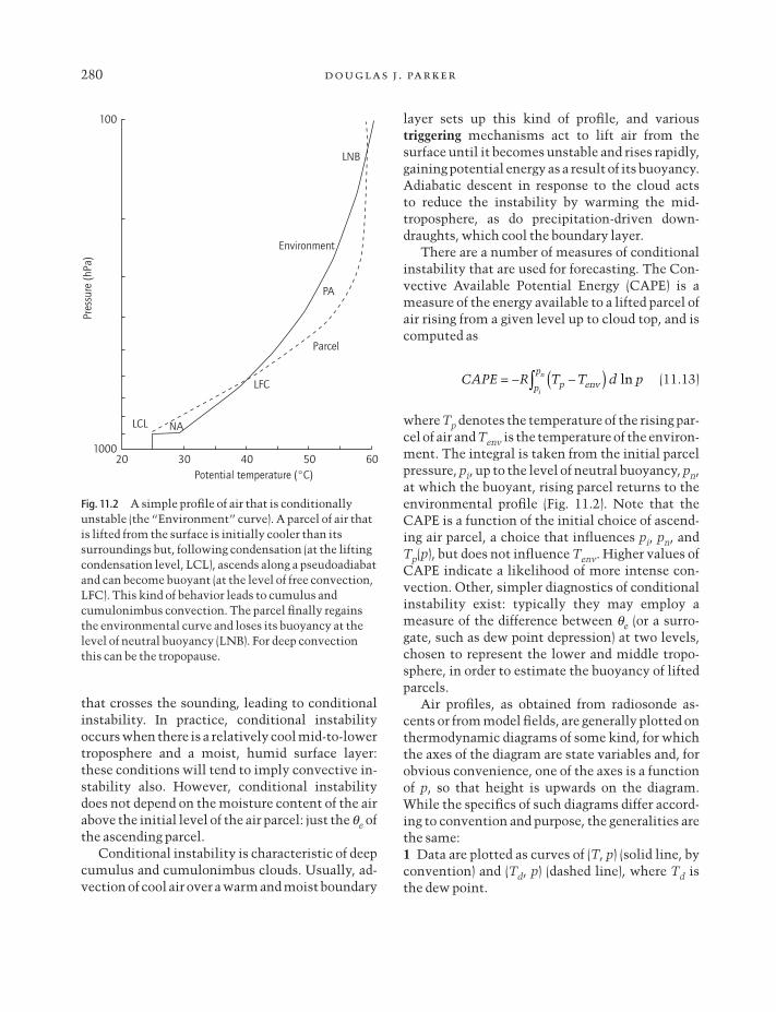
2 Adiabats are marked on the diagram: these arethe routes that unsaturated air parcels will followin ascent or descent.3 Pseudoadiabats are also marked, to indicate thetrajectories of saturated parcels.4 Lines of constant humidity mixing ratio indicate the evolution of dew point for unsaturatedair.Given any initial air state of (p, T, Td), causing thisair to ascend to a lower pressure implies that thetemperature will evolve by following an adiabatand the dew point by following a line of humiditymixing ratio, until these meet, at which point theair is saturated. Subsequent ascent will follow apseudoadiabat. An example of the most commonlyused thermodynamic diagram in the UK, the“tephigram,” is shown in Fig. 11.3.
11.2.2 Dynamics
The discussion has so far considered a static atmosphere, and the conditions for instability ofsuch an atmosphere when parcels are displaced.The study of the full dynamic evolution of weathersystems requires a more precise description of thefluid flow. The basic equation set used to describemost atmospheric flows is the “primitive equa-tions,” which are derived as an inviscid, shallow-atmosphere approximation to the Navier–Stokesequations in spherical geometry (see Holton 1992).Molecular diffusion and viscosity terms are negli-gible on synoptic scales, due to the extremely highReynolds numbers of macroscopic atmosphericphenomena. However, it is usually necessary to include turbulent dissipation terms on the
30
.20.0
18.0
16.0
14.0
10.0
8.06.04.03.02.01.51.0.80
.60
Isobar
10501000950900850800
750
700
650
600
550
500
450
400
350
300
250
20030 40 50 60 70 80
90–8
0–7
0–6
0–5
0–4
0–3
0
–20
–10
0
10
20
–20–10
010
20Adiabat
constant q Isoth
erm
:
cons
tant
T
Consta
nt h
mr
Pseudoadiabat
Fig. 11.3 The curves of Fig. 11.2represented on a tephigram, as anexample of one of a number ofthermodynamic diagrams incommon use. By convention, thedew point curve would be plotted onthe (T, p) axes as a dashed line (notshown here). The dew point of anunsaturated air parcel follows a lineof constant humidity mixing ratioas its pressure changes.

282 douglas j . parker
right-hand side of the momentum and thermody-namic equations.
It is the primitive equations that form the basisfor numerical weather prediction (NWP) modelsand from which simpler sets are derived. For synoptic-scale flows on horizontal scales less thanthe planetary scale, these equations are commonlyapproximated to an “f-plane” or a “b-plane,” inwhich cartesian coordinates are used and the Cori-olis parameter, f = 2Wsinc (where c is the latitudeand W is the planetary angular rotation rate), is ap-proximated by a constant (f-plane; f = f0) or a linearfunction of the cartesian latitude (b-plane; f = f0 +by). In general, in the following discussions thenorthern hemisphere is assumed, so that f0 > 0.The hydrostatic approximation is also used as astandard for synoptic flows.
Often, the equations are converted to a pressurecoordinate system, (x, y, p) (see Carlson 1991).Pressure coordinates have the advantages that in-compressibility is exact in the continuity equa-tion, and that the Boussinesq approximation is notneeded in order to simplify the pressure terms, butthese coordinates yield a more complicated lowerboundary condition and the necessity of describ-ing vertical motion in terms of a less intuitive pressure tendency. Hoskins and Bretherton (1972)outlined a “pseudo height” vertical coordinate,which is a monotonically decreasing function ofpressure and approximates quite closely to physi-cal height: for simplicity of interpretation, this co-ordinate is used here. The basic working equationset is now:
(11.14)
(11.15)
(11.16)
(11.17)
(11.18)DDt
Sq
=
— ( ) =. rru 0
∂∂
=f q
qzg
0
DuDt
fuy
- =∂∂f
DuDt
fvx
- =∂∂
f
where (u, v, w) are the components of zonal, merid-ional, and vertical velocity, f is the geopotential,rr(z) is a reference density, and S is the diabaticsource term. The normal cartesian total derivativeis used. The “vertical velocity,” w, in these coordi-nates is a simple function of the pressure tendency,w, and density; w = -rgw (meaning that imposi-tion of a boundary condition related to vertical velocity on w remains an approximation). Theequations are identical to a Boussinesq, anelasticset in true height coordinates, in which case frepresents p/rr.
QG theory
The classic simplification of eqns 11.14–11.18,which applies to synoptic-scale systems and has,in many respects, defined the subject of synopticmeteorology, is to nondimensionalize and then ex-pand in the Rossby number
(11.19)
where U is a velocity scale and L a length scale. Atfirst order the expansion yields
(11.20)
(11.21)
where vg = (ug, vg) is the well known geostrophicwind, which is the horizontal wind for which theCoriolis force balances the pressure gradient force.A consequence of the force balance is that the windis directed along the isobars, causing a cyclonic circulation (same sense as the planetary rotation)around a low-pressure system and an anticycloniccirculation around a high. In fact, the geopotential,f (or in true height coordinates, the dynamic pressure, p/r), represents a streamfunction for thegeostrophic wind. The geostrophic wind may use-fully be employed to estimate wind speeds fromcharts of isobars. However, for synoptic analysisand forecasting another, deeper relationship, the
vf xg =
∂∂
1
0
f
uf yg = -
∂∂
1
0
f
RoUf L
=0
Synoptic-Scale Meteorology 283
thermal wind balance, exists. The thermal windbalance comes from combining the hydrostaticeqn 11.16 with the equations for the geostrophicwind (eqns 11.20 and 11.21) to obtain
(11.22)
(11.23)
or, in vector form
(11.24)
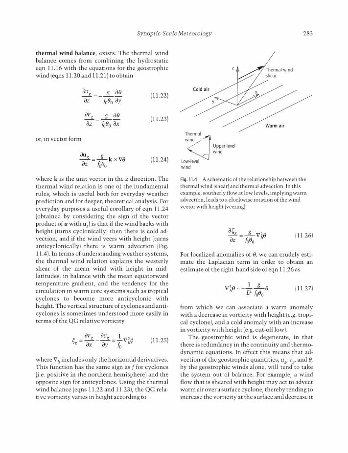
where k is the unit vector in the z direction. Thethermal wind relation is one of the fundamentalrules, which is useful both for everyday weatherprediction and for deeper, theoretical analysis. Foreveryday purposes a useful corollary of eqn 11.24(obtained by considering the sign of the vectorproduct of u with uz) is that if the wind backs withheight (turns cyclonically) then there is cold ad-vection, and if the wind veers with height (turnsanticyclonically) there is warm advection (Fig.11.4). In terms of understanding weather systems,the thermal wind relation explains the westerlyshear of the mean wind with height in mid-latitudes, in balance with the mean equatorwardtemperature gradient, and the tendency for the circulation in warm core systems such as tropicalcyclones to become more anticyclonic withheight. The vertical structure of cyclones and anti-cyclones is sometimes understood more easily interms of the QG relative vorticity
(11.25)
where —h includes only the horizontal derivatives.This function has the same sign as f for cyclones(i.e. positive in the northern hemisphere) and theopposite sign for anticyclones. Using the thermalwind balance (eqns 11.22 and 11.23), the QG rela-tive vorticity varies in height according to
x fgg g
h
v
x
u
y f=
∂∂
-∂∂
= —1
0
2
∂∂
= ¥ —u
kg
zg
f0 0qq
∂∂
=∂∂
v
zg
f xg
0 0qq
∂∂
= -∂∂
u
zg
f yg
0 0qq
(11.26)
For localized anomalies of q, we can crudely esti-mate the Laplacian term in order to obtain an estimate of the right-hand side of eqn 11.26 as
(11.27)
from which we can associate a warm anomalywith a decrease in vorticity with height (e.g. tropi-cal cyclone), and a cold anomaly with an increasein vorticity with height (e.g. cut-off low).
The geostrophic wind is degenerate, in thatthere is redundancy in the continuity and thermo-dynamic equations. In effect this means that ad-vection of the geostrophic quantities, ug, vg, and q,by the geostrophic winds alone, will tend to takethe system out of balance. For example, a windflow that is sheared with height may act to advectwarm air over a surface cyclone, thereby tending toincrease the vorticity at the surface and decrease it
— -h Lg
f2
20 0
1q
qq~
∂∂
= —x
qqg
hzg
f0 0
2
x
y
Thermal windshear
Cold air
z
Warm air
Thermalwind
Low-levelwind
Upper levelwind
Fig. 11.4 A schematic of the relationship between thethermal wind (shear) and thermal advection. In thisexample, southerly flow at low levels, implying warmadvection, leads to a clockwise rotation of the windvector with height (veering).
284 douglas j . parker
aloft (thermal wind relation). Such changes in vorticity can only occur through ageostrophic motion, such as vertical velocity stretching thesurface vorticity. Hence in order to describe thetime-evolution of the geostrophic winds, it is nec-essary to consider the Ro expansion further (i.e.consider an expansion of the form
(11.28)
where uag is the “ageostrophic” zonal wind, andtake terms in O(Ro)). To next order in Ro we obtainthe quasigeostrophic (QG) equations (“quasi” because they include the effect of an ageostrophicwind), which are the basis for an understanding ofsynoptic weather systems:
(11.29)
(11.30)
(11.31)
(11.32)
(11.33)
where the geostrophic Lagrangian derivative is
(11.34)
N2(z) is a function of the basic state, reference tem-perature profile, and small products of uag and bhave been neglected. It is also useful to construct aQG vorticity equation for the vertical componentof the geostrophic vorticity, zg = f + xg,
(11.35)D
Dtf
zwg
gr
rzr ∂
r( ) =∂ ( )0
D
Dt tu
xv
yg
g g=∂∂
+∂
∂+
∂∂
D
Dtw
gN Sgq q
= - +0 2
rr∂r
ag ag ru
x
v
yw
z
∂∂
+∂∂
ÊËÁ
ˆ¯̃
+∂( ) = 0
∂∂ q
qu
kg
zg
f= ¥ —
0
D v
Dtf u yug g
ag g+ + =0 0b
D u
Dtf v yvg g
ag g- - =0 0b
u u Ro u O Rog ag= + ¥ + ( )2
From eqn 11.35 it can be seen that the principaltendency in geostrophic absolute vorticity is dueto convergence or divergence leading to vortexstretching in the vertical. This highlights the im-portance of the ageostrophic wind in QG dynam-ics: the only way to derive a tendency in thegeostrophic fields is through ageostrophic motion.
There are two useful ways of simplifying theQG equation set. The first and perhaps more obvi-ous is to combine these equations in a form thateliminates time derivatives and leaves ageostro-phic terms on the left-hand side, as flows forced by geostrophic terms on the right: this leads to the well known “omega equation” (or, for two-di-mensional flows, the equivalent Sawyer–Eliassenequation). The second route is equally useful andinvolves eliminating ageostrophic terms altogeth-er, to obtain evolution equations for a geostrophicvariable, the QG potential vorticity (PV), whichhas a profound role in synoptic meteorology.
Diagnosing the ageostrophic wind: the omegaequation. Combining eqn 11.35 with eqn 11.33,using the thermal wind balance (eqn 11.26) toeliminate time derivatives, gives a single equationfor ageostrophic vertical velocity, w:
(11.36)
This equation is generally known as the omegaequation, since in true pressure coordinate form itwould be used to solve for the pressure tendency, w.It has the form of:
(11.37)
where L is a linear differential operator and F is aforcing operator that is dependent on geostrophicstreamfunction F = f/f0. The boundary conditionon w is the kinematic boundary condition of zeronormal flow at the lower surface, or a pressure ten-
L w F[ ] = [ ]F
N w fz z
w fz
gf
v
zg
S
hr
r g g
h gg
h
2 202
0
0
20
0
2
1— +
∂ ( )ÊËÁ
ˆ¯̃
=∂
—( )
- — —( ) + + —
∂ r∂∂
r∂
z
qq b
∂
∂ q
u
u
.
.
Synoptic-Scale Meteorology 285
dency for w, which, for flat terrain, is often regardedto be small. From eqn 11.37, it is apparent that the ageostrophic wind is determined by thegeostrophic fields, and it is important to remainaware that the ageostrophic wind represents onlythe next order of expansion in Rossby number, notthe full departure of the wind field from thegeostrophic wind. In particular, gravity waves remain unrepresented in QG dynamics. Theageostrophic wind exists in order to maintaingeostrophic balance in a time-dependent solution.However, from a perspective of forecasting and understanding, diagnosis of vertical motionthrough forms such as eqn 11.37 is critical to ques-tions of cyclonic development and cloud formation.
The solution to eqn 11.37 depends on solutionof a second-order partial differential equation according to particular forcing, F, and boundaryconditions. In order to gain some insight into the physical meaning of this equation, it is usefulto consider different partitions of F[f] and somerule-of-thumb inversions of the operator, L. In par-ticular, for constant N and rr the height coordinatecan be rescaled to z* = (N/f)z, in which case L is theLaplacian operator. This means that we can gainsome intuition into the solution according to vari-ous forcings, from our understanding of this wellknown operator. Then, for many functions (e.g. sinusoidal), we can make the approximation that
(11.38)
where L is a length scale for the system.In the following analysis we will neglect the
term involving b in the forcing of the omega equa-tion (eqn 11.36). The traditional partition of F[F]given above is into a term involving vorticity ad-vection and another involving thermal advection,plus the diabatic source term (see Carlson (1991)for discussion of various other expressions of F[F]).The forcing may be rewritten
(11.39)
where the new terms are the vorticity advection
F f
zg g
Sh hf∂ q q
[ ] = -∂ ( ) + — ( ) + —0
2
0
2VA TA0
L w
NL
w[ ] -~2
2
(11.40)
and the thermal advection
(11.41)
These terms can be computed exactly from modeldata, but may also be estimated by eye, as in eqn11.38:
(11.42)
This approximate relationship relates upward motion to:1 A positive vertical gradient of vorticity advec-tion (VA); for instance, the advection of an upper-level vortex tends to produce upward motionahead of the vortex.2 Positive thermal advection (TA) or positive dia-batic heating (S). These latter two are in some wayintuitive, in that warming tends to cause upwardmotion, but notice that it is not thermal anomalieswhich lead to upward motion in the QG system,but the thermal tendency.
These vorticity and thermal advection termsare the ones traditionally used by forecasters.However, use of two separate forcings based ongeostrophic diagnostics that are essentially linkedthrough thermal wind balance is rather unsatisfac-tory, especially in instances where the signs ofthese forcings may be opposite. A refinement ofthe description of F[f] has been through the con-struction of Q-vectors (see Sanders & Hoskins1990). The Q-vector is defined to be
(11.43)
in which case we have
(11.44)F F[ ] = —2 .Q
Q = -+
+
Ê
Ë
ÁÁÁÁ
ˆ
¯
˜˜˜̃
g
u
x x
v
x yu
y x
v
y y
g g
g gq
∂∂
∂q∂
∂∂
∂q∂
∂∂
∂q∂
∂∂
∂q∂
0
wLN
L wLN
F
f LN z
gN
gN
S
~
~
- [ ] = - [ ]
( ) + ( ) +
2
2
2
2
02
20
20
2
F
∂∂ q q
VA TA
TA = - —ug . q
VA = - —ug g. z
286 douglas j . parker
The Q-vector field is often computed numerically,as a model diagnostic, but also may be inferred byeye from thermal and wind fields. It is possible torewrite the Q-vector in the form
(11.45)
where s is a coordinate following the q contours inthe direction of the thermal wind. Interpreting thisgeometrically, take the vector change in ug in thedirection of the thermal wind, and rotate this vec-tor 90° anticyclonically to obtain the direction ofthe Q-vector. In order to interpret Q-vectors interms of the ageostrophic response, once againthink of the simplistic inversion of the Laplacian(eqn 11.38), in which case descent is associatedwith divergence of Q and ascent is associated withconvergence of Q. Considering the continuityequation (11.17) means that low-level Q-vectorsoften point in the direction of the low-levelageostrophic wind.
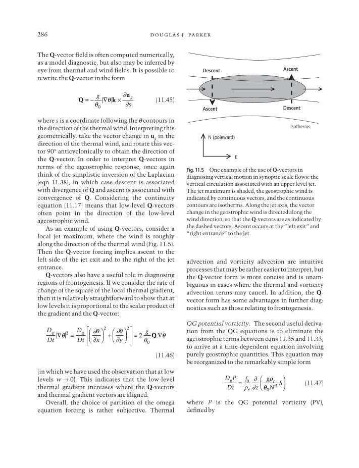
As an example of using Q-vectors, consider alocal jet maximum, where the wind is roughlyalong the direction of the thermal wind (Fig. 11.5).Then the Q-vector forcing implies ascent to theleft side of the jet exit and to the right of the jet entrance.
Q-vectors also have a useful role in diagnosingregions of frontogenesis. If we consider the rate ofchange of the square of the local thermal gradient,then it is relatively straightforward to show that atlow levels it is proportional to the scalar product ofthe gradient and the Q-vector:
(11.46)
(in which we have used the observation that at lowlevels w Æ 0). This indicates that the low-levelthermal gradient increases where the Q-vectorsand thermal gradient vectors are aligned.
Overall, the choice of partition of the omegaequation forcing is rather subjective. Thermal
D
Dt
D
Dt x ygg g— = Ê
ËÁˆ¯̃
+ ÊËÁ
ˆ¯̃
È
ÎÍÍ
˘
˚˙˙
= —q∂q∂
∂q∂ q
q22 2
02 Q.
Q ku
= - — ¥g
sg
∂∂0
advection and vorticity advection are intuitiveprocesses that may be rather easier to interpret, butthe Q-vector form is more concise and is unam-biguous in cases where the thermal and vorticityadvection terms may cancel. In addition, the Q-vector form has some advantages in further diag-nostics such as those relating to frontogenesis.
QG potential vorticity. The second useful deriva-tion from the QG equations is to eliminate theageostrophic terms between eqns 11.35 and 11.33,to arrive at a time-dependent equation involvingpurely geostrophic quantities. This equation maybe reorganized to the remarkably simple form
(11.47)
where P is the QG potential vorticity (PV), defined by
D P
Dtf
zgN
Sg
r
r=ÊËÁ
ˆ¯̃
0
02r
∂∂
rq
N (poleward)
E
Isotherms
DescentAscent
Descent Ascent
Fig. 11.5 One example of the use of Q-vectors indiagnosing vertical motion in synoptic scale flows: thevertical circulation associated with an upper level jet.The jet maximum is shaded, the geostrophic wind isindicated by continuous vectors, and the continuouscontours are isotherms. Along the jet axis, the vectorchange in the geostrophic wind is directed along thewind direction, so that the Q-vectors are as indicated bythe dashed vectors. Ascent occurs at the “left exit” and“right entrance” to the jet.
Synoptic-Scale Meteorology 287
(11.48)
in which F is the geostrophic streamfunction, F = f/f0. Thus the QG PV is conserved in adiabaticmotion. The QG PV has a profound role in atmos-pheric and oceanic dynamics, and some generaldiscussion of PV is given in Section 11.2.4. In QGsystems, eqn 11.48 can be solved (“inverted”),with suitable boundary conditions such as theNeumann boundary condition of q on the horizon-tal lower surface, to give the geostrophic stream-function, F. Knowing the geostrophic wind fieldthen allows the PV field to be advected, througheqn 11.47. Thus the PV evolution offers an alterna-tive route to solving and understanding the evolu-tion of the QG system. PV is also attractive in thatit unites the geostrophic variables in a single scalarfield: in QG dynamics, vortices are inseparably re-lated to thermal anomalies through thermal windbalance, and the PV encapsulates this (considerwriting the QG PV as
(11.49)
which expresses it as a linear function of vorticityand potential temperature). Many meteorologistsprefer to identify an atmospheric feature as a PVfeature for this reason.
Inversion of the PV equation (11.48) againbrings forward the natural height scale z*. The def-inition of z* implies a natural ratio of scales for thesystem, of L/H ~ N/f, where H is a height scale.This ratio of scales typifies many synoptic sys-tems. It also indicates a constraint on modelinggridbox sizes, if synoptic weather systems are to berepresented isotropically; the ratio of the horizon-tal to the vertical resolution of a model should ide-ally correspond to N/f. From consideration of z*, itis useful to construct a Rossby radius
(11.50)
and a Rossby height scale
(11.51)H fL NR =
L NH fR =
P f
f gz Ng
r
r= + + ÊËÁ
ˆ¯̃
xr q
∂∂
rq0
02
P f
fz N zr
r= + — +ÊËÁ
ˆ¯̃
2 02
2FF
r∂
∂r ∂
∂
to characterize the scales of influence of a given PVor omega-forcing anomaly. These are the scalesover which balanced flows tend to evolve. For in-stance, a mesoscale convective system may pro-duce a localized PV anomaly and some localizedforcing of ageostrophic motion: the geostrophicand ageostrophic flows that develop as a responseto this convective system may be expected to ex-tend over a horizontal region determined by theRossby radius, LR.
SG theory
Hoskins and Bretherton (1972) introduced semigeostrophic (SG) theory, as a refinement ofQG theory, to allow for the short length scales that occur across fronts. The basis of SG dynamicsis to define different Rossby numbers according to the across- and along-front wind and lengthscales: terms scaling with the weak across-frontwind and the large along-front length scale tend toyield low Rossby number and are negligible to firstorder. The result of this analysis is an equation setresembling the QG set, but with ageostrophicwinds explicitly in the Lagrangian derivative.Since this theory is primarily applied to frontalzones it is here presented in two dimensions, andfor an f-plane: extension to three dimensions isdocumented by Hoskins (1975). Now the basicequations are
(11.52)
(11.53)
(11.54)
(11.55)
(11.56)
where x is the cross-frontal direction and the
DDt
Sq
=
r∂
∂∂ r
∂rag r
u
xwz
+( )
= 0
Dv
Dtf ug
ag+ =0 0
gzq
q∂f∂0
=
vf xg =1
0
∂f∂

288 douglas j . parker
(11.62)
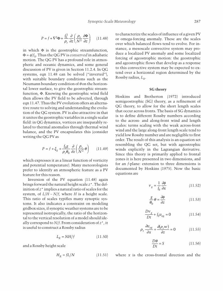
so that transforming back to physical space ef-fectively “contracts” the results in zones of highvorticity. It is this process that allows the SG equations to be useful for describing fronts, whichare amplified in regions of high vorticity. In practi-cal terms, solving numerically in geostrophicspace on a regular grid and transforming back tophysical space automatically contracts the grid inphysical space, in regions of high vorticity. Singu-lar fronts, at which there are discontinuities in thewind and temperature, evolve out of smooth initial synoptic systems at the point where the vorticity becomes singular, since in geostrophic space vorticity is a nonlinear function. There aretwo canonical large-scale flows that lead to SG frontogenesis: deformation and horizontalshear. Deformation acts to contract any tempera-ture field along its “diffluent” axis (Fig. 11.6a),while shear, as occurs in a growing baroclinicwave, for example, will produce strong gradientsalong a line of cyclonic vorticity (Fig. 11.6b). Bothmechanisms are observed, and the characteristicsof each kind of front are different: the deformationfront is more “stationary” in the flow, acting morelike a material boundary than the shear front,which generally exists as a component in a propa-gating wave, with significant across-front verticalshear of the wind.
Formally, three-dimensional SG dynamics involves the same level of approximation as QG dynamics: there is no formal reason to prefer one to the other. However, the SG equations are in two dimensions able to represent frontal zones tovery good accuracy, and for this reason they aregenerally favored for the consideration of systemssuch as the frontal cyclone, where the synoptic cy-clone develops fine-scale quasi two-dimensionalfronts. SG dynamics also leads to some other im-provements over QG, such as a physical represen-tation of the observed asymmetry between theintensity of highs and lows in a developing baro-clinic wave.
JX Y Zx y z
ff
f
v
Xg
∫ ( )( ) = =
-
∂∂
z ∂∂
, ,, ,
11
Lagrangian derivative includes advection due tothe across-front ageostrophic flow (uag, w)
(11.57)
This system is simplified by transformation togeostrophic coordinates (as distinct from the usualphysical coordinates, (x, z))
(11.58)
so that the total derivative reduces to
(11.59)
Then, after manipulation as outlined in the QGderivation above, a Sawyer–Eliassen equation (re-lated to an omega equation) can be derived for theageostrophic streamfunction.
More details of the mathematical formulationin geostrophic coordinates are given by Hoskins(1975). An equation for PV conservation is ob-tained after some quadratic terms have been neglected:
(11.60)
with the SG PV given by
(11.61)
The SG equations in geostrophic (X, Y, Z) arestructurally very similar to the QG equations inphysical coordinates (x, y, z) and in consequencethe interpretation of the solutions follows theideas outlined for QG dynamics. However, in in-terpreting the SG results, they must be trans-formed back to physical (x, y, z) space. It is thisnonlinear transformation that accounts for the influence of ageostrophic advection —the keyprocess differentiating QG and SG dynamics. Notably, the Jacobian of the transformation turnsout to be
qZ
=1r
z∂q∂
DqDt
SZ
=zr
∂∂
DDt T
uX
vY
wZg g= + + +
∂∂
∂∂
∂∂
∂∂
X Z T x v f z tg, , , ,( ) = +( )
DDt t
u ux
vy
wzg ag g= + +( ) + +
∂∂
∂∂
∂∂
∂∂
Synoptic-Scale Meteorology 289
11.2.3 Diabatic effects
Stress terms on the right-hand side of the mo-mentum equations arise from unresolved mo-mentum flux convergence. In the troposphere and stratosphere these terms appear as a result of mix-ing by convection and at significant dynamical features such as fronts or jetstreaks, or as a result of momentum flux convergence by inertia-gravitywaves. The inertia-gravity waves are oscillationson relatively high frequencies, from a synoptic perspective, and are effectively filtered out of thebalanced equation sets: they are generated at orography, as well as at weather features such as fronts and cumulonimbus systems. None of these means of imposing stresses on airflow is particularly well understood, although some attempts to represent them in numerical models are being made. However, the stresses occurring at the Earth’s surface and communicated by turbulence into the boundary layer are better un-derstood and can be discussed in relatively simpleterms.
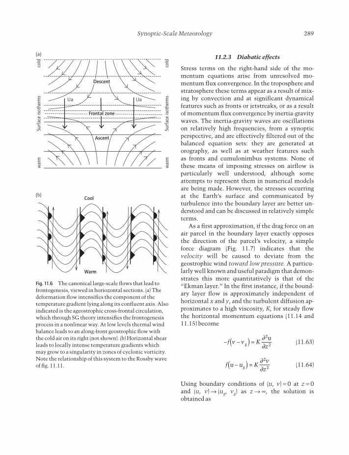
As a first approximation, if the drag force on anair parcel in the boundary layer exactly opposes the direction of the parcel’s velocity, a simple force diagram (Fig. 11.7) indicates that the velocity will be caused to deviate from thegeostrophic wind toward low pressure. A particu-larly well known and useful paradigm that demon-strates this more quantitatively is that of the“Ekman layer.” In the first instance, if the bound-ary layer flow is approximately independent ofhorizontal x and y, and the turbulent diffusion ap-proximates to a high viscosity, K, for steady flowthe horizontal momentum equations (11.14 and11.15) become
(11.63)
(11.64)
Using boundary conditions of (u, v) = 0 at z = 0and (u, v) Æ (ug, vg) as z Æ •, the solution is obtained as
f u u Kv
zg-( ) =∂∂
2
2
- -( ) =f v v Ku
zg∂∂
2
2
Surf
ace
iso
ther
ms
UaUa
Ascent
Frontal zone
Descent
(a)
cold
warm
Surf
ace
iso
ther
ms
cold
warm
Cool
Warm
(b)
Fig. 11.6 The canonical large-scale flows that lead tofrontogenesis, viewed in horiozontal sections. (a) Thedeformation flow intensifies the component of thetemperature gradient lying along its confluent axis. Alsoindicated is the ageostrophic cross-frontal circulation,which through SG theory intensifies the frontogenesisprocess in a nonlinear way. At low levels thermal windbalance leads to an along-front geostrophic flow withthe cold air on its right (not shown). (b) Horizontal shearleads to locally intense temperature gradients whichmay grow to a singularity in zones of cyclonic vorticity.Note the relationship of this system to the Rossby waveof fig. 11.11.

290 douglas j . parker
(11.65)
(11.66)
where the characteristic boundary layer depth
(11.67)
A typical value of d might be 500m. This solutionrepresents the “Ekman spiral”; for instance, if the geostrophic wind is a constant westerly wind, (ug, 0), the limiting surface wind direction is south-westerly (northern hemisphere; f > 0), and thewind vector rotates anticyclonically with heightround toward the geostrophic wind. Effectivelythis confirms that the flow under the influence ofturbulent drag deviates toward low pressure.
If the conditions are relaxed to allow for weakhorizontal gradients, the Ekman solution may be
d =
2Kf
v vz z
uz z
g g= - -ÊË
ˆ¯
ÊË
ˆ¯ + -Ê
ˈ¯1 exp cos exp sin
d d d d
u u
z zv
z zg g= - -Ê
ˈ¯
ÊË
ˆ¯ - -Ê
ˈ¯1 exp cos exp sin
d d d d
used to deduce a weak vertical motion, wE, at thetop of the Ekman layer: from continuity (eqn11.17), assuming constant density in the relativelyshallow boundary layer and integrating withheight
(11.68)
This “Ekman pumping” implies that in regions of positive relative vorticity there is upward motion forced at low levels. The upward motion iscompensated by a vertical “squashing” of the air in the troposphere, leading to a reduction in the relative vorticity (from eqn 11.35). In effect, theboundary layer stresses on the airflow extract ener-gy from a cyclone through this Ekman pumpingmechanism, and this is a way in which vor-tices (positive or negative relative vorticity) spin down under the influence of boundary layer vis-cous effects.
The turbulence in the boundary layer can be astrong function of the solar heating at the surface,in which case K can fall suddenly at nightfall to asmall value. Then, the Coriolis force acting on theair in the boundary layer is no longer balanced by turbulent dissipation terms and leads to an acceleration
(11.69)
(11.70)
the solution of which is an “inertial oscillation” offrequency f (Fig. 11.8). The effect of this oscillationis to cause the wind direction to fluctuate duringthe night, at the altitudes where there had been asignificant departure of the horizontal wind fromthe geostrophic value, usually in the lower hun-dreds of meters above the ground. Notably the am-plitude of the wind increases with time in the earlystages of the oscillation and at some point in thecycle it will exceed the geostrophic wind. This ac-celeration of the wind speed at sunset is referred toas the “nocturnal jet.”
ddvt
f u ug+ -( ) = 0
ddut
f v vg- -( ) = 0
w E g=
dx
2
Low
PGF
Isobars
Dragforce
Coriolisforce
V
High
Fig. 11.7 A schematic of the force balance when drag isopposed to the wind direction, leading to a turning of thewind vector towards low pressure.

Synoptic-Scale Meteorology 291
From the omega equation (11.36) it can be seenthat a positive diabatic heating, S, will tend to forcepositive vertical motion (from a naive inversion ofthe Laplacian operators, as in eqn 11.38), as wouldbe expected. The influence on the PV is a positivePV source below the level of maximum heatingand a negative PV source above (in some sensesthere is no real PV source (Haynes & McIntyre1987, 1990), merely a PV redistribution, and thevolume-integrated PV remains constant unlessthere are boundary sources). The net effect on theair passing through the region of latent heating de-pends crucially on the airflow structure: if the airsimply flows upwards in the region of heating, itgains PV at lower levels and loses it aloft, leading toa PV maximum at midlevels (Fig. 11.9a). If, in contrast, the heating is short-lived, or the air ispassing horizontally through the region of heating,low-level air gains positive PV and upper-level air gains negative PV, as in the squall line models of Hertenstein and Schubert (1991) or Parker and Thorpe (1995) (Fig. 11.9b). The situation assketched in Fig. 11.9b is really rather complicated:individual parcels of air may descend in the unsaturated environment of convective cells,
Period 1/f
u
ug
Fig. 11.8 The inertial oscillation: when drag retards thewind it tends to turn toward the left (NH). If this dragsubsequently diminishes, the wind vector describes aninertial oscillation about the geostrophic wind vector.At some point in the cycle, this leads to a windmagnitude exceeding that of the geostrophic wind.
PV
Negativesource
High
Positivesource
(a)
(b)
LowPV
HighPV
Meanmotion
Fig. 11.9 Schematics of the relationship betweenpropagation and PV sources for diabatic heating in aconvective system. In (a) the source is stationary; as airascends in the convective clouds it gains PV at lowlevels to generate a positive anomaly. Above the level ofmaximum heating the PV source becomes negative andthe resulting PV structure is a single positive anomaly atmid-levels. In (b) the source is moving, and air parcelspass though the PV sources from left to right (dashedlines represent air parcel trajectories and continuouslines show the mean air motion). Low-level air gainspositive PV and upper-level air gains negative PV on thelarge scale. The resulting PV structure is a dipole in thevertical.

292 douglas j . parker
ascend rapidly within the cells themselves, or evendescend rapidly in the downdraughts of storms.The response of the large-scale, averaged state tothis convection is not well understood, but wouldtypically correspond to a large-scale mean heatingwith a structure related to that within an individ-ual cumulonimbus.
Closing the system by coupling the cloud dia-batic sources to the synoptic dynamics is one of thepoorly understood meteorological problems. Somevery simple models have used a modified “CISK”parametrization, to specify the heating as a func-tion of boundary layer convergence (calculatedfrom the ageostrophic winds, which are them-selves forced by the latent heating, or from the boundary-layer convergence), in a represen-tation of “triggered” convection. However, the atmospheric horizontal scales over which trigger-ing is the controlling process are thought to be re-stricted to the mesoscale; perhaps pertaining tofrontal convection on tens of kilometers but not towidespread convection over hundreds of kilome-ters in the cold sector of a frontal cyclone, for example.
Other simple parametrizations have employedan assumption of near-neutral stability to con-vection, in which case there is a heat source pro-portional to the local value of (upward) verticalmotion, which leads to a reduced (but still positive)effective static stability. If a negative effective sta-bility occurs, the various inversion operators forthe balanced systems (e.g. L[w] for the omega equa-tion) change their properties significantly, by ceas-ing to be elliptic. In particular, it is possible thenfor the solutions to lose uniqueness, in which case“free” solutions may be obtained, and the resultsare not in general well determined.
Neither of the above approaches to representingcloud diabatic processes is ideal, and there is someevidence that more than one parametrization mayneed to be combined if realistic representations areto be achieved (Lagouvardos et al. 1993). Opera-tional NWP models split clouds into large-scale,resolved clouds and subgrid convective clouds.This split reflects physical differences in cloudform and origin (stratiform versus convective), aswell as being a practical necessity for modeling
with a finite horizontal resolution. The opera-tional convective parametrization may be dealtwith in a variety of ways, and its implementationhas a strong bearing on the results of global numer-ical models, largely because of the impact of moistconvection on tropical dynamics. Increasing com-puter power has meant progressively finer numeri-cal grids, and we are now at the stage where theresolution of models is close to the scales of convective systems, and such systems are beingneither resolved nor parametrized.
11.2.4 More on PV
Study of dynamical meteorology has in recentyears been suffused with the concept of potentialvorticity, yet many meteorologists, in particularsome practicing forecasters, remain skeptical as tothe usefulness of PV in real analysis. In this light,the important properties of PV are reviewed here.PV is often regarded as a rather mysterious quanti-ty, shrouded in subtle mathematics: while it is truethat the mathematics behind PV dynamics can be deep, the fundamentals of PV behavior are quite intuitive, given some basic knowledge of thedynamics.
Hoskins et al. (1985) (HMR) highlighted the twoaspects of PV analysis that make it useful: its con-servation and its invertibility. Conservation isexact in adiabatic, inviscid flows, even for the fullinviscid Navier–Stokes equations, in which case
(11.71)
where z is the absolute vorticity vector. If the at-mosphere approximates adiabatic conditions (typ-ically over times of many hours or a few days) thePV is a dynamical tracer for the air. It is the dynam-ical part of this that particularly fascinates theo-reticians; the fact that there is a tracer whichreflects properties of the wind field. For practicalpurposes the basic state structure of PV in the at-mosphere makes conservation particularly useful:the PV becomes large in the stratosphere due to thehigh static stability above the tropopause, andtherefore anomalies in PV at upper levels (and even
P = —1r
z q.
Synoptic-Scale Meteorology 293
descending to the surface in tropopause folds) re-flect material motion of air of stratospheric andtropospheric origin. When correlated with tracegases such as water vapor or ozone, the PV candemonstrate deep links between the chemistryand the dynamics of the atmospheric flow. In mid-latitudes the dynamical tropopause, often definedto lie at PV = 2 PVU (1.0 or 1.5 PVU are also com-monly used, where the PV unit is defined as 1 PVU= 10-6 m2 Kkg-1 s-1; see HMR) has become widelyused in diagnostic studies, as this is approximatelya material surface whose evolution can be fol-lowed through time.
Plotting the PV on an isentropic surface is oftenpreferred to plotting PV on height or pressure sur-faces, since the isentropic surface is approximatelya material surface. This means that PV anomaliescan credibly be tracked in two dimensions withoutconcern for motion out of the plane (except in regions of significant diabatic processes).
Invertibility implies that the flow field can bereconstructed from a knowledge of the PV (withsuitable boundary conditions), and it is this proper-ty that gives PV real practical usefulness in under-standing the evolution of weather systems. Inorder for the PV to be invertible, there must besome balance condition on the flow fields (HMR),and such a condition (thermal wind balance) is es-sential to the QG and SG theories underpinningsynoptic analysis. Heuristically the PV may be in-verted “by eye,” especially in cases of large hori-zontal scale where the vertical component of thethermal gradient is dominant: in such cases, PV approximates by
(11.72)
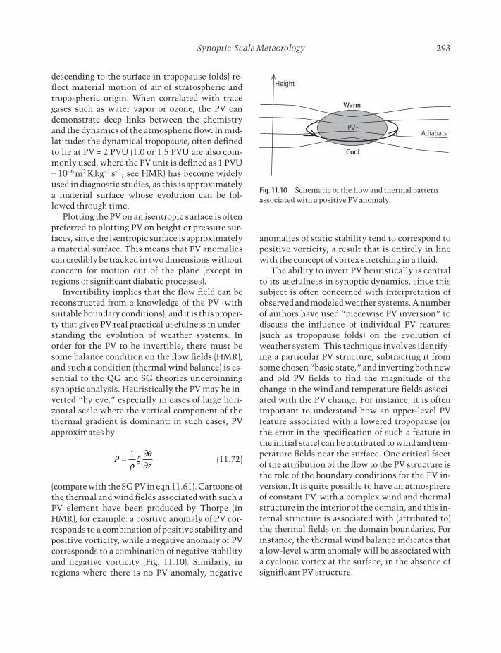
(compare with the SG PV in eqn 11.61). Cartoons ofthe thermal and wind fields associated with such aPV element have been produced by Thorpe (inHMR), for example: a positive anomaly of PV cor-responds to a combination of positive stability andpositive vorticity, while a negative anomaly of PVcorresponds to a combination of negative stabilityand negative vorticity (Fig. 11.10). Similarly, in regions where there is no PV anomaly, negative
Pz
=1r
z∂q∂
anomalies of static stability tend to correspond topositive vorticity, a result that is entirely in linewith the concept of vortex stretching in a fluid.
The ability to invert PV heuristically is centralto its usefulness in synoptic dynamics, since thissubject is often concerned with interpretation ofobserved and modeled weather systems. A numberof authors have used “piecewise PV inversion” todiscuss the influence of individual PV features(such as tropopause folds) on the evolution ofweather system. This technique involves identify-ing a particular PV structure, subtracting it fromsome chosen “basic state,” and inverting both newand old PV fields to find the magnitude of thechange in the wind and temperature fields associ-ated with the PV change. For instance, it is oftenimportant to understand how an upper-level PVfeature associated with a lowered tropopause (orthe error in the specification of such a feature inthe initial state) can be attributed to wind and tem-perature fields near the surface. One critical facetof the attribution of the flow to the PV structure isthe role of the boundary conditions for the PV in-version. It is quite possible to have an atmosphereof constant PV, with a complex wind and thermalstructure in the interior of the domain, and this in-ternal structure is associated with (attributed to)the thermal fields on the domain boundaries. Forinstance, the thermal wind balance indicates thata low-level warm anomaly will be associated witha cyclonic vortex at the surface, in the absence ofsignificant PV structure.
Height
Warm
Cool
PV+Adiabats
Fig. 11.10 Schematic of the flow and thermal patternassociated with a positive PV anomaly.

294 douglas j . parker
One way of relating the thermal boundary con-ditions to “PV thinking” is through the “Brether-ton analogy” (Bretherton 1966), whereby a warmanomaly on the lower boundary is equivalent to aninfinitesimal layer of positive PV anomaly and awarm anomaly on an upper boundary is equivalentto an infinitesimally thin layer of negative PVanomaly. In consequence, warm anomalies nearthe ground tend to act like positive PV, and are usually associated with positive vorticity: this isan observation that could equally well be madethrough direct consideration of the thermal windrelation. However, seeing boundary thermal ano-malies in PV terms allows us to understand Rossby waves on the surface in terms of simpletheory, as will be seen in Section 11.2.5.
An example of the power of considering suchbalanced flows in PV terms is that of an elevatedzone of latent heating. It is known that such heat-ing leads to a PV source within the heating zonethat is proportional to the vertical gradient of theheating: a positive source below the heating maxi-mum and a negative source above it. In conse-quence, in the absence of strong vertical motion,the response to propagating heating is a PV dipole;positive below negative (Fig. 11.9b). The heuristicinversion of this PV structure, as outlined above,implies a thermal structure that represents a warmanomaly between the PV anomalies (in the regionof maximum heating, as required). Also, each ele-ment in the dipole may be associated with a vortexat that level. This latter observation demonstrateshow the PV analysis encapsulates more than a sim-ple thermal analysis, because it contains the ther-mal wind balance condition within its definition.From a knowledge of heating, a source term in thethermodynamic equation, we have deduced PVsource terms, and thereby a wind structure that isguaranteed to be in balance with the new thermalfield. This process could have been deduced by in-voking the thermal wind balance directly from thethermal anomaly, but the PV inversion methoddeals with balance implicitly.
In overview, provided that we know a balancecondition, the properties of conservation and in-vertibility together mean that the atmosphericevolution can be described purely in PV terms: a
knowledge of the PV at a given instant allows us toinvert to get the flow fields. These flow fields maythen be applied to advect the conserved PV to pro-duce an evolving atmospheric state. In practice,many balanced (QG or SG) models do follow thisprogram of PV conservation and inversion.
Beyond its fundamental role as a conserved dynamical quantity that encapsulates a balancecondition, PV is also useful as a diagnostic of at-mospheric stability. Thinking intuitively onceagain, with PV being simply the product of stabili-ty and vertical vorticity, it can be seen that nega-tive PV generally corresponds to negative staticstability (static instability) or negative vorticity(implying inertial instability). As shown byHoskins (1974), this association of negative PVwith instability is a necessary condition for sym-metric instability, which may occur in practice inregions where the flow is neither statically unsta-ble nor inertially unstable, in their pure forms. Par-cel theory has shown that the relative slopes ofisentropes and surfaces of constant angular mo-mentum, M = vg + fx, determines an equivalentcondition for symmetric instability: the instabili-ty may be manifest where the isentropes are steeper than the momentum surfaces.
The derivation of the conservation relation forPV requires that there is a thermodynamic quanti-ty, q, which is a single-valued function of p and r.Consequently there is an infinite number of otherpotential vorticities which could be constructed:the use of q is chosen to make invertibility a usefuland intuitive process. In consideration of flowswhere latent heating or cooling is active, the wet-bulb potential temperature (qw, homeomorphic toqe) is often used as a more exactly conserved fieldthan q. Because of this, a wet-bulb potential vortic-ity, PVw, is often invoked, and this is widely used asa diagnostic of moist symmetric instability. How-ever, it must not be forgotten that qw used to calculate PVw is not a thermodynamic variable, de-pending on the three variables, p, r, and humidity,so the PVw field is neither conserved nor invertible(qw does not determine buoyancy unless the air issaturated). Examples of the nonconservation ofPVw are given by Cao and Cho (1995) and Parker(1999).

Synoptic-Scale Meteorology 295
11.2.5 Rossby waves
Having developed an understanding of balancedflows and in particular the role of PV in QG dy-namics, it is now possible to discuss the most fun-damental mode of variability of the synoptic-scaleatmosphere; the Rossby wave (see Gill 1982 for amore complete discussion). Rossby waves occurwhere there is a gradient in PV, or a gradient in tem-perature at the ground (which may be seen as a PVgradient, using the Bretherton analogy of Section11.2.4). For the sake of argument we may considera discrete boundary between zones of differing PV,on which is superposed a wavelike disturbance(Fig. 11.11). Where there is an incursion of high PVinto the lower PV area, we anticipate (from aheuristic PV inversion) a cyclonic anomaly of cir-culation, and where the lower PV intrudes into thehigher PV, anticyclonic circulation occurs. The re-sult of these circulations is a wavelike flow acrossthe PV gradient that is out of phase with the PVanomalies. By eye, it can be seen that the flowacross the gradient will tend to cause the PV waveto propagate, and the resulting propagating wave isthe essence of a Rossby wave. For the climatologi-cal northward PV gradient in mid-latitudes, due tothe meridional gradient of the Coriolis parameter,Rossby waves propagate westwards relative to theflow: in the westerly jets the net result is eastwardpropagation of Rossby waves at upper levels. Incontrast, the equatorward temperature gradient inmid-latitudes means that Rossby waves at the sur-face tend to propagate eastwards. An interactionbetween upper- and lower-level Rossby waves
leads to a positive feedback, with the circulation ofthe upper and lower waves reinforcing each other,and this mechanism is the basis behind baroclinicinstability (see HMR).
For the purposes of conceptual understanding, arelatively simple barotropic Rossby wave can beconsidered. Consider two-dimensional QG flow,independent of latitude, y, on a b-plane, underbarotropic conditions of zero horizontal tempera-ture gradient. Since the Q-vector is identicallyzero, there is no vertical motion, and the vorticityequation (11.35) reduces to
(11.73)
where U0 is a uniform zonal wind. Writing thegeostrophic streamfunction in modal form, with ka wavenumber and w a frequency, leads to the dis-persion relation
(11.74)
From consideration of the phase speed
(11.75)
it can be seen that such Rossby waves on the plan-etary vorticity gradient, b, propagate westwardsrelative to the mean flow. However, as notedabove, given that the mid-latitude flow is domi-nated by the westerly jets, upper-level Rossbywaves tend to propagate eastwards relative to thesurface. There is also an important possibility ofstationary waves.
In other contexts, the relevant (potential) vor-ticity gradient may be reversed from the gradientin Coriolis parameter. For instance, the mean pole-to-Equator temperature gradient at the surface im-plies an equivalent negative PV gradient, throughthermal wind balance or the Bretherton analogy.Easterly jets, such as the African Easterly Jet, canalso exhibit reversed PV gradients. Work by Snyderand Lindzen (1991) and Parker and Thorpe (1995)has discussed the role of sources of PV due to latent
c
kU
k= = -
w b0 2
w
b= -U k
k0
∂∂
∂∂
∂∂
∂∂
b∂∂t x
Ux x x
2
2 0
2
2 0F F F
+ + =
High PV
Low PV
Fig. 11.11 Schematic of a Rossby wave on a boundarybetween two regions of differing PV. The thick contourdenotes the interface between the regions and thedashed contour is the subsequent position of thisinterface. Other arrows indicate the circulation inducedby the waves on the interface.
296 douglas j . parker
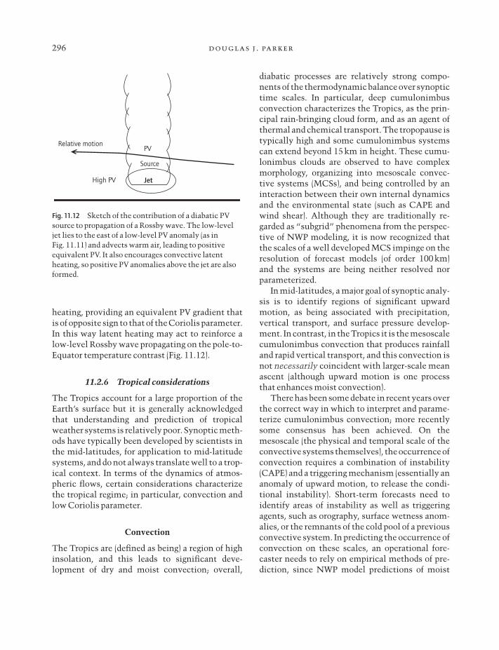
heating, providing an equivalent PV gradient thatis of opposite sign to that of the Coriolis parameter.In this way latent heating may act to reinforce alow-level Rossby wave propagating on the pole-to-Equator temperature contrast (Fig. 11.12).
11.2.6 Tropical considerations
The Tropics account for a large proportion of theEarth’s surface but it is generally acknowledgedthat understanding and prediction of tropicalweather systems is relatively poor. Synoptic meth-ods have typically been developed by scientists inthe mid-latitudes, for application to mid-latitudesystems, and do not always translate well to a trop-ical context. In terms of the dynamics of atmos-pheric flows, certain considerations characterizethe tropical regime; in particular, convection andlow Coriolis parameter.
Convection
The Tropics are (defined as being) a region of highinsolation, and this leads to significant deve-lopment of dry and moist convection; overall,
diabatic processes are relatively strong compo-nents of the thermodynamic balance over synoptictime scales. In particular, deep cumulonimbusconvection characterizes the Tropics, as the prin-cipal rain-bringing cloud form, and as an agent ofthermal and chemical transport. The tropopause istypically high and some cumulonimbus systemscan extend beyond 15km in height. These cumu-lonimbus clouds are observed to have complexmorphology, organizing into mesoscale convec-tive systems (MCSs), and being controlled by an interaction between their own internal dynamicsand the environmental state (such as CAPE andwind shear). Although they are traditionally re-garded as “subgrid” phenomena from the perspec-tive of NWP modeling, it is now recognized thatthe scales of a well developed MCS impinge on theresolution of forecast models (of order 100km) and the systems are being neither resolved nor parameterized.
In mid-latitudes, a major goal of synoptic analy-sis is to identify regions of significant upward motion, as being associated with precipitation,vertical transport, and surface pressure develop-ment. In contrast, in the Tropics it is the mesoscalecumulonimbus convection that produces rainfalland rapid vertical transport, and this convection isnot necessarily coincident with larger-scale meanascent (although upward motion is one processthat enhances moist convection).
There has been some debate in recent years overthe correct way in which to interpret and parame-terize cumulonimbus convection; more recentlysome consensus has been achieved. On themesoscale (the physical and temporal scale of theconvective systems themselves), the occurrence ofconvection requires a combination of instability(CAPE) and a triggering mechanism (essentially ananomaly of upward motion, to release the condi-tional instability). Short-term forecasts need toidentify areas of instability as well as triggeringagents, such as orography, surface wetness anom-alies, or the remnants of the cold pool of a previousconvective system. In predicting the occurrence ofconvection on these scales, an operational fore-caster needs to rely on empirical methods of pre-diction, since NWP model predictions of moist
Relative motionPV
Source
JetHigh PV
Fig. 11.12 Sketch of the contribution of a diabatic PVsource to propagation of a Rossby wave. The low-leveljet lies to the east of a low-level PV anomaly (as in Fig. 11.11) and advects warm air, leading to positiveequivalent PV. It also encourages convective latentheating, so positive PV anomalies above the jet are alsoformed.

Synoptic-Scale Meteorology 297
convection are generally unreliable. Typically theforecaster may use the model predictions of windsand thermodynamic fields to make a prediction of convection based on local knowledge and the recent history of convective storms.
On larger temporal and spatial scales, theprocess of triggering may be relatively rapid, andconvection may be seen as being in a sustainedequilibrium with the radiative forcing (primarilyshortwave heating at the surface and longwavecooling aloft). The convective systems act to warmthe middle to upper troposphere and cool theboundary layer (reduce its qe) through materialtransport in downdraughts. On these larger scalesthe problem in understanding and predicting theconvective cloud distribution is to quantify the re-lationship between the energy budgets in the equi-librium state. For instance, the low-level qe maydetermine the thermal profile aloft, through a convective equilibrium condition (such as a requirement of zero CAPE). The low-level qe isthen determined by a balance between surfacefluxes (determined by low-level winds and sea sur-face temperatures over the ocean; very much morecomplex over land), boundary layer entrainment,and convective downdraughts (themselves relatedto the complex morphology of the convective sys-tems). The wind fields that partially control thesefluxes are dependent on the thermal and pressurestructures set up by the radiative–convective equilibrium.
In all, the discussion in terms of theradiative–convective equilibrium has proposedthat for large-scale convective fields, triggering by large-scale upward motion is not the primarycontrol on the clouds. In general, the large-scalevertical motion is relatively weak, and the rapidupdraughts in storms are to a great extent compen-sated by subsidence in the clear air. Individual convective systems respond to their local environ-mental conditions: instability, wind shear, andtriggering mechanisms. The convective stormsthen act to modify and control the large-scale ther-mal state and it is this large-scale thermal fieldthat, through associated pressure gradients, leadsto large-scale horizontal and vertical motions. Tounderstand how the large-scale wind fields feed
back on the convective field, we need to take intoaccount the feedbacks on the energy balance between the troposphere and the boundary layer.On the large scale, then, the role of upward motionis not to trigger convection but to modify the ther-modynamic profile. Whereas in mid-latitudes amajor goal of synoptic analysis is to diagnose areasof ascent, which are likely to lead to precipitation,in the Tropics large-scale ascent is just one factorcontrolling the stability of the profile and the occurrence of rainfall.
As remarked above, the line between resolvedand subgrid convection is not clear. Althoughequilibrium assumptions are favored for manylarge-scale models, they may not be appropriate tomany synoptic circumstances, in which the con-vection operates close to the scale of the synopticvariability. For instance, in the monsoon over sub-Saharan West Africa, high CAPE is common, andan equilibrium state seems inappropriate: the con-vection seems to occur intermittently, every fewdays, as an interaction between the synoptic struc-ture of CIN and triggering by orography or surfacewetness. Once formed, convective systems overWest Africa may propagate as coherent storms formany hours (comparable with the time scale ofsynoptic variability) and may significantly modifytheir synoptic environment.
Coriolis force
As we approach the Equator, the Coriolis parame-ter approaches zero and the Coriolis force becomesnegligible. At the Equator there is no possibility ofgeostrophic balance, so any horizontal pressuregradient must either be balanced by frictional dragor lead to an acceleration of the air.
Much of the tropical zone is dominated by thelow-level trade winds, which flow down the pres-sure gradient toward the climatological low pres-sure associated with the ITCZ, and are turned bythe Coriolis force to give them an easterly compo-nent. When the ITCZ departs from the Equator andone branch of the trades is moving poleward, awesterly component develops. Climatologically,easterlies are observed at low levels near the Equa-tor, but the zonal mean picture masks consider-

298 douglas j . parker
able variations around the globe and westerlies arenot uncommon.
As a consequence of the low Coriolis force,strong horizontal temperature gradients are rarenear the Equator. Moving a few degrees poleward,however, the strength of the insolation means that significant temperature gradients can be sus-tained: a notable example is the monsoon overWest Africa in the summer months, in which thereis a marked transition between high temperaturesover the Sahara and lower temperatures over thetropical Atlantic Ocean. This thermal transition is accompanied by a wind shear which is qualita-tively in thermal wind balance, and leads to the African Easterly Jet at about 600–700hPa and alatitude of 10–20°N. Tropical cyclones are alsosensitive to the Coriolis parameter, and are there-fore not formed within around 5° of the Equator.Consequently, in the Tropics there is no simple,immediate separation of the dynamics accordingto geostrophically balanced flow. It has been saidthat all tropical flows are mesoscale phenomena,since no terms in the equations can automaticallybe negelected.
On the Equator, the b-plane approximation (f =by) is a relatively good one. A common treatmentis to linearize the equations of motion on the b-plane and separate variables into a vertical struc-ture function and a horizontal structure satisfyingthe equations for a shallow homogeneous layer(Gill 1982, chapter 6). Within this framework, theexistence of the gradient in planetary vorticity expressed through b leads to the possibility ofwestward-propagating Rossby waves (Gill 1982,chapter 11). Another possibility of wave dynamicsat the Equator is through eastward propagation ofKelvin waves. The Kelvin wave solution is one forwhich the meridional wind, v, is identically zero:in this case by considering the meridional momen-tum equation we have on the Equator
(11.76)
The result is that, for the Kelvin wave, high pres-sure on the Equator is associated with westerliesand low pressure with easterlies. The zonal mo-
uy
= -1 2
2b∂ f∂
mentum equation then implies that the westerlieswill accelerate on the eastern side of a high-pressure anomaly, leading to eastward propagation of a disturbance. A final wave solution near theEquator (apart from inertia-gravity modes) is theRossby-gravity wave (see Gill 1982, p. 440): thiswave has the behavior of a gravity wave for highpositive wave number and a Rossby wave for highnegative wave number, while its group speed is always eastward. This mode exhibits the possibili-ty of a stationary solution (with eastward grouppropagation).
A key result in consideration of forced solutionsnear the Equator is obtained from the steady, lin-earized vorticity equation (see Gill 1982, p. 465),and states that vertical stretching is associatedwith poleward motion,
(11.77)
a relationship that is connected with “Sverdrupbalance” for the ocean (and note the relationship to the b term in the omega equation (11.36). These ideas now allow us to infer the response of the tropical atmosphere to localized heating: the composition of the westward-propagating Rossby wave response and eastward-propagatingKelvin wave response has led to a well known“Matsuno–Gill” model of the effects of tropospheric heating close to the Equator (say as aresult of changes in the convective field, due toboundary layer qe changes). The form of this re-sponse for symmetric heating is a pair of low-levelcyclonic circulations to the west, straddling theEquator, and easterlies to the east (as shownschematically in Fig. 11.13). To the east, this response is due to Kelvin wave propagation withzero meridional flow and easterly winds at low levels. Around the longitude of the heating, thelower tropospheric vertical vorticity is stretchedand the low-level air moves polewards, in accor-dance with eqn 11.77. Some compensating equa-torward flow occurs to the west, as a result ofRossby wave propagation. Similar results for heating that is located away from the Equator arediscussed by Gill (1982).
b∂∂
v fwz
=

Synoptic-Scale Meteorology 299
11.3 APPLICATIONS TOWEATHER SYSTEMS
Synoptic meteorology had its origins and very def-inition in the resolution of observations that wereavailable to the analyst. In recent times, the use ofthose observations has passed to the electroniccomputer, which assimilates the data into a previ-ous forecast field to generate an analysis of greaterhorizontal resolution than the observation set. Inaddition to this, the computer model is now diag-nosing weather patterns (precipitation, turbu-lence, etc.), at its given resolution, explicitly. Thismeans that the boundary between synoptic mete-orology and mesoscale meteorology is in practicebecoming blurred: synoptic meteorology may stillbe defined as that involving scales well repres-ented by balanced theories, but the practicing forecaster is routinely analyzing weather patternson much finer scales than the synoptic observingnetwork.
11.3.1 Frontal cyclones
The most deeply studied atmospheric weather sys-tem is undoubtedly the frontal cyclone, and thebasic model of this object is centered on balanceddynamics. It was constructed by the Bergen school
of V. Bjerknes and co-workers around the end of theFirst World War and the mid-latitude frontal cyclone (Fig. 11.14a) remains the most well knownand well studied of synoptic phenomena, largelybecause of its importance to the developed nationsin Europe and North America, but also because ofits significance as a very coherent structure in thecomplexity of nonlinear atmospheric flow. Expla-nations of the dynamics and evolution of such cyclones have evolved to some extent, and it isnow appreciated that the Norwegian model on itsown is inadequate to describe some complex as-pects of the cyclone, such as its transport proper-ties. Some refinements in the Norwegian modelare indicated in Fig. 11.14.
The Bergen school originally identified frontalcyclones as unstable growing waves on a “polarfront.” Although a coherent polar front is not identified in global analyses, it remains true thatthese cyclones represent baroclinic instabilities of the basic pole-to-Equator temperature contrast,extracting potential energy from the basic state and converting it to potential and kinetic en-ergy of the cyclone. The baroclinic zone on whichthe cyclones grow is typically marked by westerlywind shear with height (through the thermal wind relation), leading to an upper tropospheric jetassociated with a change in tropopause height (e.gFig. 11.15). Thus the location of the jetstream is an important indicator of the baroclinic zone,apart from importance in its own right as a windfeature.
The cyclogenesis process was first accuratelyunderstood in terms of linear QG instability models (Charney 1947; Eady 1949; discussed byGill 1982 and HMR), which identified the cyclonesas components of an unstable baroclinic wave. Theidealized Eady wave in particular may be seen as aperiodic sequence of highs and lows as a result ofRossby waves at upper and lower levels. For suit-ably long wavelengths, the upper and lower wavesare able to couple and lead to an exponentiallygrowing wave: the lows of the upper wave augmentthe cyclonic flow at lower levels and vice versa.The tilt of the cyclone with height turns out to bewestwards for unstable waves, which is a usefulguide for interpreting upper- and lower-level
Equator
L
L
Fig. 11.13 A schematic of the low-level response toheating located symmetrically across the Equator. The heating region is shaded and upward motionapproximately matches this zone. The response to thewest is a pair of low-pressure centers with correspondingcyclonic circulation, while easterlies occur to the east.The meridional scale of this response is controlled by anequatorial Rossby radius related to b and stability,typically of the order of 1000 km.

Tropopause
Convectivecloud
Drydescent
Jet
Surfacefront
(c)
L
(a)
Surfacefront
Jet
Stratiformcloud
(b) Cirrus
Fig. 11.14 The classical Norwegian cyclone model and some more recent refinements. Note that fronts are plotted onthe warm air side of each frontal zone. (a) Isobars and fronts in a typical alignment; a “kink” in the isobars at each front is related to locally increased low-level vorticity. (b) The warm front is characterized by stratiform cloud,decreasing in depth ahead of the front. The jet (into the section) in the cold air ahead of the front is related to the cold conveyor belt and decreases with height according to thermal wind balance. (c) A classical cold front ischaracterized by convective clouds and a narrower, more intense band of precipitation than anticipated at a warm front. The low-level jet ahead of the front (into the section) is related to high low-level PV due to latent heatingand/or a band of warm air at low levels ahead of the cold front; the jet is linked to the warm conveyor belt. There iscommonly a stronger jet along the front at the tropopause level, with a significant change in tropopause height at thefront (the tropopause may often form a “fold” in the descending zone behind the front as indicated here). (Continued)
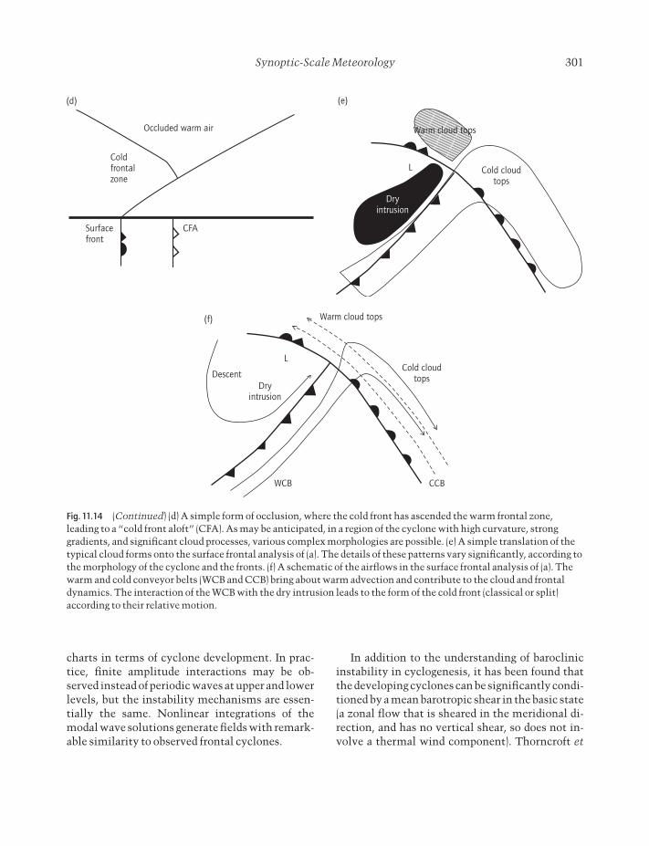
Synoptic-Scale Meteorology 301
charts in terms of cyclone development. In prac-tice, finite amplitude interactions may be ob-served instead of periodic waves at upper and lowerlevels, but the instability mechanisms are essen-tially the same. Nonlinear integrations of themodal wave solutions generate fields with remark-able similarity to observed frontal cyclones.
In addition to the understanding of baroclinicinstability in cyclogenesis, it has been found thatthe developing cyclones can be significantly condi-tioned by a mean barotropic shear in the basic state(a zonal flow that is sheared in the meridional di-rection, and has no vertical shear, so does not in-volve a thermal wind component). Thorncroft et
Coldfrontalzone
Occluded warm air
Surfacefront
CFA
(d)
Warm cloud tops
Cold cloudtops
L
Dryintrusion
(e)
DescentDry
intrusion
Warm cloud tops
Cold cloudtops
CCB
L
WCB
(f)
Fig. 11.14 (Continued) (d) A simple form of occlusion, where the cold front has ascended the warm frontal zone,leading to a “cold front aloft” (CFA). As may be anticipated, in a region of the cyclone with high curvature, stronggradients, and significant cloud processes, various complex morphologies are possible. (e) A simple translation of thetypical cloud forms onto the surface frontal analysis of (a). The details of these patterns vary significantly, according tothe morphology of the cyclone and the fronts. (f) A schematic of the airflows in the surface frontal analysis of (a). Thewarm and cold conveyor belts (WCB and CCB) bring about warm advection and contribute to the cloud and frontaldynamics. The interaction of the WCB with the dry intrusion leads to the form of the cold front (classical or split)according to their relative motion.

302 douglas j . parker
al. (1993) have studied idealized life cycles of suchdeveloping cyclones and discussed two paradigms,LC1 and LC2, which have enjoyed some signifi-cant attention. Very superficially, the two life cycles are distinguished by an enhanced cyclonicshear in the basic state of LC2, which leads to a cyclonic wrapping-up of the upper-level trough to produce a significant upper-level cut-off cycloneat high latitudes. Hoskins and West (1979) andDavies et al. (1991) have discussed the influence ofsuch barotropic shear on the frontal structure:large-scale shear of the zonal wind with latitudeacts to control the relative intensities of the coldand warm fronts (cyclonic shear, as in LC2, en-hances warm frontogenesis), as well as some fundamental aspects of the airflow patterns.
The basic observational picture of fronts con-structed as part of the Bergen cyclone model re-mains relatively unchanged: the cold front followsthe warm front, and they bound the warm sector.Where these fronts merge, one may undercut theother, leading to an occlusion. The classical warmand cold fronts are sketched in Fig. 11.14b and c:the warm front is characterized by more stratiform
types of cloud and precipitation, while the coldfront tends to be steeper and exhibit cumulonim-bus convection. Such a cold front is now termed a“classical” cold front, to distinguish it from a lessintuitive, but relatively common, form of “splitcold front.” At a split cold front (Fig. 11.16), there issignificant advection through the frontal zone,leading to the advance of a layer of dry air above thesurface cold front. At the nose of this dry air is anupper cold front, at which cumulonimbus convec-tion may occur, and the whole zone between theupper and lower cold fronts is characterized byconditional instability. Consideration of the splitfront demonstrates that it is impossible to regardthe fronts as airmass boundaries: these pheno-mena act as steep waves in the airflow, which mayor may not be stationary relative to the air locally.There is significant along-front thermal advection(naturally, since the frontal cyclone as a whole iscomposed of propagating Rossby waves), whichmay contribute to the frontal propagation. The re-sults of Parker (1999) indicate that the occurrenceof the split cold front may be favored in systemswith a relatively low steering level, for which thereis stronger upper-level cross-frontal advection,while classical cold fronts occur in baroclinic
Cool
Polewards Equatorwards
Warm
Adiabats
Tropopause
Jet
Fig. 11.15 A meridional cross-section through themidlatitude westerly jet, indicating its relationship withthe thermal pattern (through thermal wind balance) andwith the tropopause. The location of the jetstream isthen coincident with the zone of thermal and PVgradients, which give rise to instability in the form offrontal cyclones.
Dry
Warm cloudtops
Jet
Fig. 11.16 Schematic of a split cold front, in which dryair overruns the surface cold front, possibly associatedwith a dry intrusion.

Synoptic-Scale Meteorology 303
models with stronger upper-level control, a highersteering level, and consequently weaker cross-frontal flow in the mid-troposphere.
The upper fronts associated with a split coldfront may on occasion propagate right across thewarm frontal zone, leading to a propagating rain-band at the normally stratiform warm front (e.g.Browning et al. 1995). Another form of upper coldfront is the “cold front aloft,” which occurs at awarm occlusion, where the cold front is rising overthe warm frontal zone, but may remain coherent atupper levels (Fig. 11.14d). Locatelli et al. (1994)have related such upper-level features to signifi-cant weather patterns at the surface. In general, the nature of the occlusion is a matter of some disagreement and certainly exhibits considerablevariability. Some authors have argued in terms of a“bent-back warm front” to describe the evolvingsurface thermal pattern in certain systems. “Occlusion” refers to the lifting of the warm air between the converging cold and warm fronts, while the term “seclusion” refers to the cutting offof a pool of warm air, polewards of the main warmsector.
Advection of dry air above the surface cold frontis normally associated with a dry intrusion of airdescending from the poleward direction, behindand then above the cold front. Such dry intrusionstend to be very clear in WV imagery and may be as-sociated with stratospheric air, of high PV andozone concentrations, being brought almost downto the surface (Fig. 11.14e and f). At the cold front,the destabilizing effect of the advection of dry air atlow- to mid-levels in the dry intrusion is enhancedby warm advection from the equatorward direc-tion ahead of the cold front in a “warm conveyorbelt” (Fig. 11.14f), which is related to the low-leveljet observed ahead of cold fronts (Fig. 11.14c). Fromthermal wind balance at a simple cold front (asconstructed in simple dry models such as the “de-formation front”), one would expect low-levelalong-front flow with the cold air on its right, incontrast to the direction of the observed jet aheadof the cold front. This jet is observed to be associat-ed with a low-level warm band ahead of the frontand/or with PV anomalies at low levels generatedby latent heating in the frontal clouds. The warm
advection in the warm conveyor belt may be im-portant in the frontal propagation (Browning &Pardoe 1973), as it is associated with the surfaceRossby wave, and certainly acts to increase theconditional and convective instability that leadsto the cumulonimbus convection at the cold front.The term “conveyor belt” was coined in the late1960s and tends to imply a material flux of air fromthe equatorward direction, being carried polewardand ascending as it approaches the center of the cyclone. Theoretically speaking, identification ofthe cyclone as a propagating wave tends to suggestthat it may be more reasonable to see the conveyorbelt as an Eulerian rather than a Lagrangian fea-ture, with air parcels entering the warm conveyorbelt from the east before ascending above the coldfront. However, case study analyses of air parceltrajectories in mid-latitude cyclones (Wernli 1997)have indicated that in the active part of the cyclonethe conveyor belts may indeed act as coherent Lagrangian features, with air parcels remainingwithin the conveyor belt throughout their passage along the frontal zone.
A “cold conveyor belt” has also been identified(Fig. 11.14f) in the cold air ahead of the warm front.Both the warm and the cold conveyor belts,through bringing about warm advection, may na-turally be linked to the high vorticity that mustoccur in a frontal zone (from SG theory, or theBretherton analogy).
Another important consequence of the convec-tion that commonly occurs at the cold front is thepossibility of boundary layer uplift. In such casesthe cold front may resemble a squall line at whichthe surface front behaves like a gust front, or a lab-oratory density current (see review by Smith &Reeder 1988). The low-level cold air at the frontlifts the warm sector boundary layer air off theground, and undercuts it with cleaner, colder airproduced in convective downdraughts (Browning& Harrold 1970). The combination of dry intru-sions of stratospheric air into the middle and lowertropopause with rapid lifting of warm sectorboundary layer air means that cold fronts make asignificant contribution to larger-scale chemicaltransport.
In the Bergen cyclone model, the distinct

304 douglas j . parker
airmasses separated by the fronts have distinctweather characteristics. More recently theseweather characteristics of the different sectorshave been identified with the evolution of stabilityproperties due to differential advection in differentsectors of the wave, rather than to the history ofdistinct masses of air. In particular, Parker (1999)has discussed the evolution of qe in simple baro-clinic waves and shown that this can account forsome of the observed weather characteristics.Basic state profiles of qe tend to have less verticalvariation than the q profiles, because of the capa-city of the warmer lower-level air to hold morewater vapor. This means that in areas of descend-ing air from the poleward direction (“downglid-ing” air; HMR) the convective stability tends to bereduced: a mid-level maximum in descending,equatorward flow leads to significant mid-level reduction in qe, while q is compensated throughadiabatic warming. Such behavior is characteristicof the air behind the cold front, regardless of thesurface over which it passes.
Frontal cyclones are known to grow as insta-bilities of the mid-latitude baroclinic zones, andnaturally the cold and warm fronts within thesecyclones may also be unstable, to secondary cy-clones (see review by Parker 1998). Such cyclonesare generally of smaller scale (say 500km) and may grow very rapidly (occasionally into severeweather systems), making them extremely im-portant yet difficult to forecast. A great deal of recent research effort has been directed at under-standing these secondary systems, and some basicconclusions are now reasonably well accepted:1 Like the parent cyclones, the secondaries maydevelop as baroclinic waves. However, there is also a strong or even dominant component of baro-tropic instability (feeding off the basic state kinetic energy) at these scales. The relative im-portance of barotropic and baroclinic instabilitydepends on the geometrical structure of the PVanomalies at the front.2 Most fronts are unstable to secondary cyclonegrowth, but few exhibit intensely growing cy-clones. This may be due to the rapid saturation ofunstable linear modes in the nonlinear regime, orto the effect of frontogenesis processes (the large-
scale flows in the parent cyclone leading to an unsteady, time-dependent front) in suppressing instability in many cases.3 Moist processes become more important onshorter horizontal length scales, and there is evi-dence that secondary cyclones may receive signifi-cant energy from cloud feedbacks.
11.3.2 Mountains
Flow influenced by hills and mountains is of greatimportance in global climatology and in the deter-mination of local weather patterns. The horizontalscales of surface orography range from the conti-nental scales downwards, and the way in whichthe atmosphere responds to such features dependson the relevant scales of wind speed, height,length, and Coriolis parameter. The principal con-trolling parameters are the Rossby number (eqn11.19) and the Froude number
(11.78)
where H is the mountain height scale.
Low Rossby number flow
Here the nature of the flow is interpreted in termsof balanced (e.g. QG) dynamics. The basic responseof the atmospheric column as it passes over themountains is to be “squashed” in the vertical andthereby, from the QG vorticity equation, to form a relative anticyclone. Less obviously, the air col-umn may tend to stretch before it reaches the hilland in the lee of the hill, to generate a low upstreamand downstream (Fig. 11.17). Lee lows in particularare common features of various parts of the world,such as northern Italy in the lee of the Alps. The superposition of the anticyclone and cyclonesmeans more intense anticyclonic winds associat-ed with the hill. Upstream, these winds are relatedto barrier winds: close to a steep hill where there isa pressure gradient along the contours or orogra-phy, there can be little Coriolis force to balance thepressure gradient (the horizontal flow up the hill isrestrained by stability) and the flow tends to follow
Fr
UNH
=
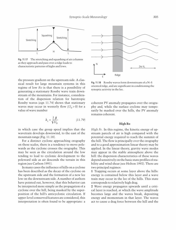
Synoptic-Scale Meteorology 305
the pressure gradient on the upstream side. A clas-sical result for large mountain systems in thisregime of low Ro is that there is a possibility ofgenerating a stationary Rossby wave train down-stream of the mountains. For instance, considera-tion of the dispersion relation for barotropicRossby waves (eqn 11.74) shows that stationarywaves may occur in westerly flow (U0 > 0) for avalue of wave number
(11.79)
in which case the group speed implies that thewavetrain develops downwind, to the east of themountain range (Fig. 11.18).
For a distinct cyclone approaching orographyon these scales, there is a tendency to move pole-wards as the cyclone crosses the orography. Thismay be seen as the circulation around the lowtending to lead to cyclonic development to thepoleward side as air descends the terrain in this region (see Carlson 1991).
In many cases the influence of hills on a cyclonehas been described as the decay of the cyclone onthe upstream side and the formation of a new leelow on the downstream side. A number of authorshave pointed out, however, that this behavior canbe interpreted more simply as the propagation of acyclone over the hill, being masked by the super-position of the hill’s anticyclonic circulation. Ifupper-level conserved features are considered, thisinterpretation is often found to be appropriate: a
kUs =b
0
coherent PV anomaly propagates over the orogra-phy and, while the surface cyclone may tempo-rarily be masked over the hills, the PV anomalyremains coherent.
High Ro
High Fr. In this regime, the kinetic energy of up-stream parcels of air is high compared with the potential energy required to reach the summit ofthe hill. The flow is principally over the orographyand to a good approximation linear theory may beapplied. In the linear theory, gravity wave modesmay appear in the stable atmosphere above thehill: the dispersion characteristics of these wavesdepend sensitively on the basic state profiles of sta-bility and wind shear (see Holton 1992). There aretwo principal regimes:1 Trapping occurs at some layer above the hills:energy is contained below this layer and a wavetrain may occur in the lee of the hills. This statecorresponds to relatively high drag.2 Wave energy propagates upwards until a criti-cal layer is reached, at which the wave amplitudebecomes large and the waves break, depositing energy and momentum in that layer. The wavesact to cause a drag force between the hill and the
Stretching
SquashingStretching
L LH
Fig. 11.17 The stretching and squashing of air columnsas they approach and pass over a ridge leads tocharacteristic patterns of highs and lows.
N
E
2p/ks
Ridge
Fig. 11.18 Rossby waves form downstream of a N–Soriented ridge, and are significant in conditioning thesynoptic activity in the lee.

306 douglas j . parker
atmosphere, through a vertical flux of horizontalmomentum, and in order that the drag be of the right sign (tending to decelerate the airflow)the wave crests tilt upstream with height. This tilt of the waves tends to lead to a confluence of the streamlines on the downwind side of the hill (Fig. 11.19), which implies a speed-up of the flow in the lee. This effect is also forced by nonlinear effects in the airflow, and downslopewindstorms are relatively common hazards ofhilly areas.
Low Fr. For typical values of N and U, this regimeis somewhat extreme for the atmosphere, but inlight winds and conditions of high stability, low-Frconditions may be observed at high mountains.The basic balance is that the kinetic energy of airupstream is significantly less than the potentialenergy required to reach the summit: in this casethere must be flow splitting and a stagnation point.For the case of long ridges there may be damming ofthe low-level air, which is unable to ascend theridge, and strong barrier winds may occur on theupslope side.
11.3.3 Tropical cyclones
Tropical cyclones are among the most severe andhazardous of weather patterns, with the potentialto devastate shipping and coastal land areas,through a combination of high winds, extreme seastate, and heavy precipitation. They occur over the
tropical oceans and although they may pass overland, they cannot persist without the latent heatfluxes from the ocean. In the Atlantic, intensetropical cyclones are known as “hurricanes,” andin the Pacific they are called “typhoons”; weakercyclones are termed “tropical depression,” in-creasing in intensity to “tropical storm,” and cy-clones are named once they reach tropical stormstrength. Tropical cyclones are routinely observedand their progress is predicted with a variety ofmodeling techniques. However, forecasting of themovement of the storms remains imperfect andthe storm dynamics is an area of active research.
Initiation of tropical cyclones is known to depend on several criteria:1 A warm core precursor vortex is needed.2 The sea surface temperature must be greaterthan 26°C.3 The tropospheric wind shear must be relativelyweak.4 There must be a decrease of qe with height in thelower troposphere, and a humid mid-troposphere.5 The latitude must correspond to significantCoriolis parameter (so these storms do not formwithin 5° of the Equator).Once formed, tropical cyclones are maintainedthrough the strong sensible and latent heat fluxesfrom the ocean, which are amplified by the coolingof air as it moves in toward the very low pressure atthe center. The cyclones exhibit a warm core, cor-responding, through eqn 11.26, to a decrease in theamplitude of vorticity with height and an anticy-clone at the tropopause. This warm core is main-tained by latent heat release in the convectiveclouds.
It is a common mistake to observe hurricaneforce winds (as defined on the Beaufort Scale) in amid-latitude cyclone, and consequently describethe cyclone as a hurricane. Mid-latitude cyclonesderive their energy from baroclinic mechanisms(involving horizontal temperature gradients andassociated thermal wind shear) and barotropicmechanisms (extracting energy from horizontalwind shear), which lead to particular structuresand weather patterns, such as strong axial asym-metry, and fronts. Hurricanes, in contrast, extractenergy from the warm sea surface in a quasi-
Hill
Streamlines
Upstream tilt
Fig. 11.19 The upstream tilt of gravity waves withheight occurs in order to balance momentum fluxes atthe ground: its result is a tendency for higher winds inthe lee. Downslope winds are also related to nonlineareffects in the flow.
Synoptic-Scale Meteorology 307
axisymmetric manner. While many hurricanesmay “recurve” —for example, northward along theeastern seaboard of North America —they in-evitably interact with mid-latitude baroclinicityand westerly wind shear, to become essentiallybaroclinic storms. One remote cousin of the hurri-cane that may affect the mid-latitude oceans, how-ever, is the mesoscale “polar low,” which in asignificant proportion of cases may derive its energy from relatively high fluxes from the sea sur-face into extremely cold polar airflows.
11.4 ON AIRMASSES
A widely used and abused concept in atmosphericscience is that of the “airmass”; a term that mayvariously refer to wide bodies of the atmosphereseparated by fronts, or to small volumes of air withparticular trace chemical contents. Many dynami-cal meteorologists dislike the use of this term: herean attempt is made to discuss the applicability ofthe idea of an airmass, and the more precise termi-nology that may be applied.
Within general fluid flows, it is known that relatively simple large-scale flow fields may leadto distortion of a tracer field to extremely shortscales and complex structures. For example, a vol-ume of air that is 100m deep, in a shear of 5ms-1
km-1, which is typical for the mid-latitude tropo-sphere, will after 1 day be sheared over 50km. Inturbulent flow fields, the tracer dispersion is morerapid and comprehensive, and in fully developedturbulence, any two adjacent elements of the fluidwill ultimately become separated by an arbitrarydistance in the flow. Reference is often made to a“parcel” of fluid, which is a small volume of fluidthat moves as a coherent fluid element: this is aconstruct that enables us to imagine the complexprocesses involved in real fluid flows. For example,we consider the forces on a fluid “parcel” in deriv-ing the Navier–Stokes equations, despite knowingthat such parcels could not be experimentally con-structed or observed. Similarly, one might con-sider the chemical reactions occurring in a parcelof air as it moves through the atmosphere: in reality volumes of air are being stretched and
sheared until they are dispersed widely, but provid-ed that our mentally constructed parcel of air issmall enough, it will remain coherent over thetime we wish to consider. It might be said that theparcel represents an infinitesimal volume of fluid,which may still describe physical evolution. Thedanger of employing the term “airmass” in thiscontext is that it may be taken to imply a relativelylarge volume of air (as is often the case in discus-sion of synoptic systems), which in practice willnot behave as a coherent mass of air except oversufficiently short time scales. The term “airmass”should here be used with the same reservationsand caution employed in discussing a “parcel” offluid.
“Airmasses” were invoked in the constructionof the Norwegian model, and for many years frontswere still regarded as boundaries between largezones of air of differing properties. More recently ithas been realized that the fluid dynamics of the at-mosphere is generally not well described by suchdiscrete models. At a given instant a front will very often separate regions in which the air hascharacteristically different properties, but the airin these regions is not static and is generally evolving under considerable vertical shears andhorizontal strains. This is to say that the propertiesof a column of air within an “airmass” are deter-mined by the relative advection at each level with-in that column. It is important to accept that theairmass model only works well as an instanta-neous one, and is not good for describing the evolu-tion or transport of dynamical or tracer fieldswithin those airmasses. There remain some usefulempirical descriptions of weather types in terms of airmasses, but for the purposes of describing atmospheric evolution and transport it would bebetter to work in terms of stability theory: in considering a horizontally homogeneous airmasswe are really considering a one-dimensional col-umn of the atmosphere. Transposing airmass arguments into arguments relating to an atmos-pheric column means that we can reintroduce theimportant processes of vertical shear of horizontaladvection into the model.
A significant example of the failure of airmassconcepts to describe synoptic evolution is in the
308 douglas j . parker
case of a cold front for which cross-frontal flow issignificant: an airmass model of a front cannotadmit this behavior. Reeder and Smith (1988) have described observations of such fronts overAustralia, and related them usefully to the SGfrontal model. Parker (1999) has used such SGmodels to describe the evolution of tracer fields ina frontal zone and highlighted the importance ofcross-frontal advection.
11.5 PRACTICALITIES: HOW TOPERFORM A SYNOPTIC ANALYSIS
In many instances it is useful to perform a synopticanalysis; for instance, when considering a casestudy of a pollution event or a case of severe weather. Performing such an analysis is a matterinvolving a certain amount of experience and issometimes regarded as a black art by those not reg-ularly experienced in looking at synoptic data.Certainly it is true that there is an almost limitlessamount of general information and intuition thatis built up by bench forecasters over their careers.However, it is also true that much of the informa-tion required to describe the synoptic situationsuccinctly can be obtained by routine methods.This is particularly true in the age of informationtechnology, when recent observations as well asthe results of explicit NWP models are available tomost of us through the internet. In particular, theNWP products offer detailed maps of fields such asprecipitation, which were formerly inferred by theforecaster on the basis of experience and diagnosticrules.
Practice and experience at looking at synopticdata can be gained through use of the internet andconsultation of textbooks (such as Bader et al.1995). What follows is not a definitive guide to analyzing a synoptic situation but a checklist oftopics that may bear on the analysis and should beconsidered.
11.5.1 Synoptic charts
The traditional surface chart showing isobars,lows, highs, fronts, troughs, and perhaps thickness
contours (Section 11.2.1) is usually the startingpoint for synoptic discussion. Application of thestandard paradigms of cold and warm fronts, for ex-ample, and the overall cyclone structure indicatesthe form of the weather patterns. The geostrophicwind may be inferred from the isobars and, in com-bination with the thickness pattern, this indicatesthe sense of the thermal advection. Interpretationbeyond this level of detail becomes more difficultfor the nonpractitioner: the weather associatedwith fronts in winter may be significantly differentto that in summer, for example, and varies accord-ing to location. Confirmation of the details of theweather patterns should be inferred from othercorroborative sources.
Upper air plots, apart from their immediate importance for upper-level applications such asaircraft forecasting, are useful in determining sta-bility and cyclone structure. It is common to usecharts of geopotential height of a pressure surface(say the 200hPa height): a low-pressure anomalyon a height level corresponds, conveniently, to lowheight of a pressure surface. Such upper-levelcharts are useful in indicating the vertical tilt of cy-clones, as an indication of their potential for baro-clinic growth, as well as the location of upper-leveljetstreams, associated with baroclinicity and aforcing of low-level cyclonic development (Baderet al. 1995).
11.5.2 Imagery
Use of satellite imagery improves with practice,but with some thought the basic IR and VIS chan-nels can immediately give information about thesynoptic situation.1 The VIS (visible) image gives quite intuitive information about the nature of the reflecting surface for solar radiation: white features may becloud, fog, or snow, while the sea surface and vari-ous land surfaces are relatively dark. Thin cloudssuch as cirrus may sometimes appear opaque.2 The IR image indicates the temperature of theupper surface of the emitting layer: the tops ofclouds appear cold, according to altitude, while theland surface appears warm and cold according tothe diurnal cycle. The convention is to shade this

Synoptic-Scale Meteorology 309
image with cold features white, so that high cloudtops are white, low clouds are grey, and theland/sea surface is usually dark.3 The water vapor (WV) image of geostationarysatellites is slightly more difficult to interpret, butroughly speaking this indicates the height abovewhich the atmosphere becomes relatively dry.When there has been significant descent at upperlevels, this leads to a dry upper troposphere and theWV image is shaded dark. In regions of high uppertropospheric water vapor the image is shadedwhite.4 The so-called “channel 3” image (polar-orbitingsatellites) detects radiation in a band consisting ofboth shortwave solar radiation scattered backfrom Earth (which dominates the signal during theday) and longwave radiation emitted from terres-trial sources (which dominates at night). Thechange in the source by day or night leads to aswitch-over in the appearance of sources: coldcloud tops, for example, emit relatively little radiation but may scatter solar radiation stronglyby day. For this reason, the negative is commonlyproduced for daytime images, and labeled with aminus sign: channel 3-. Some sophisticated use ofchannel 3 is outlined by Bader et al. (1995), but the principal use of this channel for qualitativeanalysis is in diagnosis of cloud droplet sizes byday. In contrast to the visible image, the cloud albedo in channel 3- is dominated by droplet size,with large drops absorbing in this band. Thus,clouds composed of relatively large drops appeardark in channel 3-, in contrast to a bright visibleimage.
Satellite imagery fields can give an indication of the intensity (size and depth of cells) of cumu-lus/cumulonimbus in the cold sector, the nature ofa cold front (split/classical), and the relative inten-sity of cold and warm fronts. The IR channel andthe WV channel in particular give striking views ofa dry intrusion. The imagery is also useful for con-firming the nature of rather poorly defined featuressuch as troughs, occlusions, and frontal waves.
Radar imagery is useful in locating precipita-tion to high spatial and temporal accuracy, espe-cially, for example, in cases of cumulonimbusconvection. Care must be taken in inferring sur-
face precipitation rates from radar estimates,which are made in an elevated section that ascendsaway from each radar (see Bader et al. 1995). Forvalidation it is possible to use surface station rainfall data.
11.5.3 Synoptic observations
The raw observations, SYNOPS from surface sta-tions and TEMPS from upper air stations, are thebread and butter of the bench forecaster’s work,and are considered essential for determining thequality and details of a synoptic forecast. For spe-cific applications such as a case study, the localconditions from the nearest reporting synoptic sta-tion are of considerable importance. More signifi-cant is likely to be the nearest radiosonde ascent,which gives far more vertical resolution than oneor two horizontal charts on different levels. Quan-tities that can be obtained from the sounding include conditional or convective instability,boundary layer characteristics, thermal advection(from the turning of the wind; eqn 11.24 and ensu-ing comments), local tropopause height, cloudbase, cloud top, and freezing level.
11.5.4 Model products
Now that model analyses are becoming more easily obtained, there are large, almost bewilder-ing, amounts of diagnostics available. The avail-ability of explicit fields of convective rainfall, forexample, can answer what were hitherto difficultquestions of interpretation without any discus-sion. However, it remains important to under-stand and interpret the situation in terms oftraditional (e.g. QG) paradigms; the interaction ofhighs and lows and thermal advection. A key ad-vantage of model diagnostics is that PV is oftenprovided explicitly, giving a useful conserved fieldwith the key dynamical role in synoptic dynamicsthat is discussed above. All this said, the explicitnature of model output means that presentation ofsuch diagnostics rarely includes coherent struc-tures such as fronts (Hewson 1998), and it is left to the user to infer these on the basis of the modelfields, the imagery, and a large dash of experience.
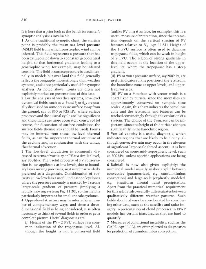
310 douglas j . parker
It is here that a prior look at the bench forecaster’ssynoptic analysis is invaluable.1 As on a traditional synoptic chart, the startingpoint is probably the mean sea level pressure(MSLP) field from which geostrophic wind can beinferred. This field represents a pressure that hasbeen extrapolated down to a constant geopotentialheight, so that horizontal gradients leading to ageostrophic wind, for example, may be inferredsensibly. The field of surface pressure is used inter-nally in models but over land this field generallyreflects the orography more strongly than weathersystems, and is not particularly useful for synopticanalysis. As noted above, fronts are often not explicitly marked on presentations of this data.2 For the analysis of weather systems, low-leveldynamical fields, such as u, q and qe or qw, are usu-ally discussed on some pressure surface away fromthe ground, say at 850 or 925hPa, where surfaceprocesses and the diurnal cycle are less significantand these fields are more accurately conserved (ofcourse, for discussion of surface conditions thesurface fields themselves should be used). Frontsmay be inferred from these low-level thermalfields, as can the important thermal structure ofthe cyclone and, in conjunction with the winds,the thermal advection.3 The low-level circulation is commonly dis-cussed in terms of vorticity or PV at a similar level,say 850hPa. The useful property of PV conserva-tion is less applicable at low levels, due to bound-ary layer mixing processes, so it is not particularlypreferred as a diagnostic. Consideration of vor-ticity at low levels is a useful indicator of cycloneswhere the pressure anomaly is masked by a stronglarger-scale gradient of pressure (implying a rapidly moving system; Fig. 11.20), so this field isparticularly important for smaller-scale cyclones.4 Upper-level structure may be inferred in a num-ber of complementary ways, and since a three-dimensional field is being considered, it is oftennecessary to think of several fields in order to get acomplete picture. Useful diagnostics are:
(i) Height of the PV = 2 PVU surface is a com-mon indication of the tropopause level. Al-though the height is not a conserved field
(unlike PV on a q surface, for example), this is auseful measure of interaction, since the interac-tion depends on the vertical spacing of PV features relative to HR (eqn 11.51). Height of the 1 PVU surface is often used to diagnosetropopause folds, which can be weak in height of 2 PVU. The region of strong gradients in this field occurs at the location of the upper-level jet, where the tropopause has a steep gradient.(ii) PV or q on a pressure surface, say 200hPa, areuseful indicators of the position of the jetstream,the baroclinic zone at upper levels, and upper-level vortices.(iii) PV on a q surface with vector winds is achart liked by purists, since the anomalies areapproximately conserved on synoptic timescales. Again, this chart indicates the barocliniczone and the jetstream, and features can betracked convincingly through the evolution of asystem. The choice of the q surface can be im-portant, since the height of this surface changessignificantly in the baroclinic region.
5 Vertical velocity is a useful diagnostic, which indicates regions that are likely to be cloudy (al-though convective rain may occur in the absenceof significant large-scale forced ascent). It is bestconsidered on some mid-tropospheric level, suchas 700hPa, unless specific applications are beingconsidered.6 Rainfall is now also given explicitly: the numerical model usually makes a split betweenconvective (parametrized, e.g. cumulonimbusconvection) and large-scale (explicitly modeled,e.g. stratiform frontal rain) precipitation. Apart from the practical numerical requirementfor this split, it also usefully differentiates betweenqualitatively different weather patterns. Suchfields should always be corroborated by consider-ing other data, such as the satellite and radar im-agery: representation of cloud processes in NWPmodels has certain inaccuracies that are hard toquantify.7 Measures of conditional instability, such as theCAPE (eqn 11.13), are often plotted as diagnosticsfor prediction of cumulonimbus convection.
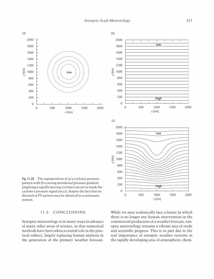
Synoptic-Scale Meteorology 311
11.6 CONCLUSIONS
Synoptic meteorology is in many ways in advanceof many other areas of science, in that numericalmethods have here taken a central role in the prac-tical subject, largely replacing human analysis inthe generation of the primary weather forecast.
While we may realistically face a future in whichthere is no longer any human intervention in thecommercial production of a weather forecast, syn-optic meteorology remains a vibrant area of studyand scientific progress. This is in part due to thereal importance of synoptic weather systems inthe rapidly developing area of atmospheric chem-
2000
1800
1600
1400
1200
1000
800
600
400
200
0
0 500 1000 1500 2000
x (km)
y (k
m)
Low
(a)
2000
1800
1600
1400
1200
1000
800
600
400
200
0
0 500 1000 1500 2000
x (km)y
(km
)
(b)
Low
High
2000
1800
1600
1400
1200
1000
800
600
400
200
0
0 500 1000 1500 2000
x (km)
y (k
m)
(c)
Low
High
Fig. 11.20 The superposition of (a) a cyclonic pressurepattern with (b) a strong meridional pressure gradient(implying a rapidly moving cyclone) can act to mask thecyclone’s pressure signal (in (c)), despite the fact that itsthermal or PV pattern may be identical to a stationarysystem.

312 douglas j . parker
istry, and in part due to the expansion of the benchforecaster’s role into prediction at ever smaller system scales. Fronts, cumulonimbus convection,and the planetary boundary layer are all phen-omena that involve the synoptic meteorologist directly, and the ways in which each modifiesweather systems and the transport of trace chemi-cals are still very poorly understood. Interpreta-tion of local events, on scales far smaller than thecomputer may resolve, will always require under-standing and interpretation of synoptic processes.At a more profound level, even if we are to reach astage where numerical weather prediction nolonger requires human intervention, most of uswould agree that it will be necessary for humans tounderstand the products of those predictions atsome real level of insight such as that provided bybalanced dynamics.
ACKNOWLEDGMENTS
In preparing this chapter I have made use of notestaken from lectures by Alan Thorpe, as well as call-ing on many helpful discussions with colleagues atthe JCMM in Reading.
REFERENCES
Bader, M.J., Forbes, G.S., Grant, J.R., Lilley, R.B.E. & Waters, A.J. (1995) Images in Weather Forecasting: A Practical Guide for Interpreting Satellite and Radar Imagery. Cambridge University Press, Cambridge.
Bolton, D. (1980) The computation of equivalent poten-tial temperature. Monthly Weather Review 108,1046–53.
Bretherton, F.P. (1966) Critical layer instability in baro-clinic flows. Quarterly Journal of the Royal Meteoro-logical Society 92, 325–34.
Browning, K.A. & Harrold, T.W. (1970) Air motion andprecipitation growth at a cold front. Quarterly Journalof the Royal Meteorological Society 96, 369–89.
Browning, K.A. & Pardoe, C.W. (1973) Structure of low-level jet streams ahead of mid-latitude cold fronts.Quarterly Journal of the Royal Meteorological Society99, 619–38.
Browning, K.A., Clough, S.A., Davitt, C.S.A., Roberts,N.M. & Hewson, T.D. (1995) Observations of themesoscale sub-structure in the cold air of a developingfrontal cyclone. Quarterly Journal of the Royal Meteo-rological Society 121, 1229–54.
Cao, Z. & Cho, H.-R. (1995) Generation of moist poten-tial vorticity in extratropical cyclones. Journal of Atmospheric Science 52, 3263–81.
Carlson, T.N. (1991) Mid-latitude Weather Systems.HarperCollins, London.
Charney, J.G. (1947) The dynamics of long waves in abaroclinic westerly current. Journal of Meteorology 4,135–63.
Davies, H.C., Schär, C. & Wernli, H. (1991) The palette offronts and cyclones within a baroclinic wave develop-ment. Journal of Atmospheric Science 48, 1666–89.
Eady, E.T. (1949) Long waves and cyclone waves. Tellus 1,33–52.
Emanuel, K.A. (1994) Atmospheric Convection. OxfordUniversity Press, Oxford.
Gill, A.E. (1982) Atmosphere–Ocean Dynamics. Acade-mic Press, New York.
Haynes, P.H. & McIntyre, M.E. (1987) On the evolutionof vorticity and potential vorticity in the presence ofdiabatic heating and frictional or other forces. Journalof Atmospheric Science 44, 828–41.
Haynes, P.H. & McIntyre, M.E. (1990) On the conserva-tion and impermeability theorems for potential vorticity. Journal of Atmospheric Science 47, 2021–31.
Hertenstein, R.A. & Schubert, W.H. (1991) Potential vor-ticity anomalies associated with squall lines. MonthlyWeather Review 119, 1663–72.
Hewson, T.D. (1998) Objective fronts. MeteorologicalApplications 5, 37–65.
Holton, J.R. (1992) An Introduction to Dynamic Meteo-rology. Harcourt Publishers, London.
Hoskins, B.J. (1974) The role of potential vorticity insymmetric stability and instability. Quarterly Journalof the Royal Meteorological Society 100, 480–2.
Hoskins, B.J. (1975) The geostrophic momentum approx-imation and the semi-geostrophic equations. Journalof Atmospheric Science 32, 233–42.
Hoskins, B.J. & Bretherton, F.P. (1972) Atmospheric fron-togenesis models: mathematical formulation and solution’, Journal of Atmospheric Science 29, 11–37.
Hoskins, B.J. & West, N. (1979) Baroclinic waves andfrontogenesis. Part II: uniform potential vorticity jetflows —cold and warm fronts. Journal of AtmosphericScience 36, 1663–80.
Hoskins, B.J., McIntyre, M.E. & Robertson, R.W. (1985)

Synoptic-Scale Meteorology 313
On the use and significance of isentropic potential vor-ticity maps. Quarterly Journal of the Royal Meteoro-logical Society 111, 877–946.
Lagouvardos, K., Lemaitre, Y. & Scialom, G. (1993) Im-portance of diabatic processes on ageostrophic circula-tions observed during the FRONTS 87 experiment.Quarterly Journal of the Royal Meteorological Society119, 1321–45.
Locatelli, J.D., Martin, J.E. & Hobbs, P.V. (1994) A widecold frontal rainband and its relationship to frontal to-pography. Quarterly Journal of the Royal Meteorologi-cal Society 120, 259–75.
Parker, D.J. (1998) Secondary frontal waves in the NorthAtlantic region: A dynamical perspective of currentideas. Quarterly Journal of the Royal MeteorologicalSociety 124, 829–56.
Parker, D.J. (1999) Passage of a tracer through frontalzones: A model for the formation of forward-slopingcold fronts. Quarterly Journal of the Royal Meteoro-logical Society 125, 1785–800.
Parker, D.J. & Thorpe, A.J. (1995) Conditional convectiveheating in a baroclinic atmosphere: a model of convec-
tive frontogenesis. Journal of Atmospheric Science 52,1699–711.
Reeder, M.J. & Smith, R.K. (1988) On air motion trajecto-ries in cold fronts. Journal of Atmospheric Science 45,4005–7.
Sanders, F. & Hoskins, B.J. (1990) An easy method for es-timation of Q vectors from weather maps. Weatherand Forecasting 5, 346–53.
Smith, R.K. & Reeder, M.J. (1988) On the movement andlow-level structure of cold fronts. Monthly WeatherReview 116, 1927–44.
Snyder, C. & Lindzen, R.S. (1991) Quasi-geostrophicwave-CISK in an unbounded baroclinic shear. Journalof Atmospheric Science 48, 78–86.
Thorncroft, C.D., Hoskins, B.J. & McIntyre, M.E. (1993)Two paradigms of baroclinic-wave life-cycle behavior.Quarterly Journal of the Royal Meteorological Society119, 17–55.
Wernli, H. (1997) A Lagrangian-based analysis of extra-tropical cyclones. II: a detailed case-study. QuarterlyJournal of the Royal Meteorological Society 123,1677–706.