hamiltonian description of the dynamics of particles in non scaling ffag machines stephan i. tzenov...

Hamiltonian Description of the Hamiltonian Description of the Dynamics of Particles in Non Dynamics of Particles in Non

Scaling FFAG MachinesScaling FFAG Machines

Stephan I. TzenovStephan I. Tzenov

STFC Daresbury Laboratory,STFC Daresbury Laboratory,

Accelerator Science and Technology CentreAccelerator Science and Technology Centre

12 – 17 April 200712 – 17 April 2007 FFAG 2007, Grenoble, FranceFFAG 2007, Grenoble, France

Contents of the PresentationContents of the Presentation

1)1) Introduction from First PrinciplesIntroduction from First Principles

2)2) The Synchro-Betatron Formalism and the The Synchro-Betatron Formalism and the Reference OrbitReference Orbit

3)3) Accelerated Orbit and DispersionAccelerated Orbit and Dispersion

4)4) The Betatron Motion and Twiss ParametersThe Betatron Motion and Twiss Parameters

5)5) The Reference Orbit and AccelerationThe Reference Orbit and Acceleration

6)6) The Phase MotionThe Phase Motion

7)7) Conclusions and Outlook Conclusions and Outlook


Introduction from First PrinciplesIntroduction from First Principles

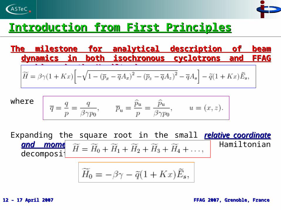
The milestone for analytical description of beam dynamics in both The milestone for analytical description of beam dynamics in both isochronous cyclotrons and FFAG machines is the Hamiltonian:isochronous cyclotrons and FFAG machines is the Hamiltonian:

where

Expanding the square root in the small relative coordinate and momentum relative coordinate and momentum variablesvariables, we have the Hamiltonian decomposition:


Introduction Continued…Introduction Continued…

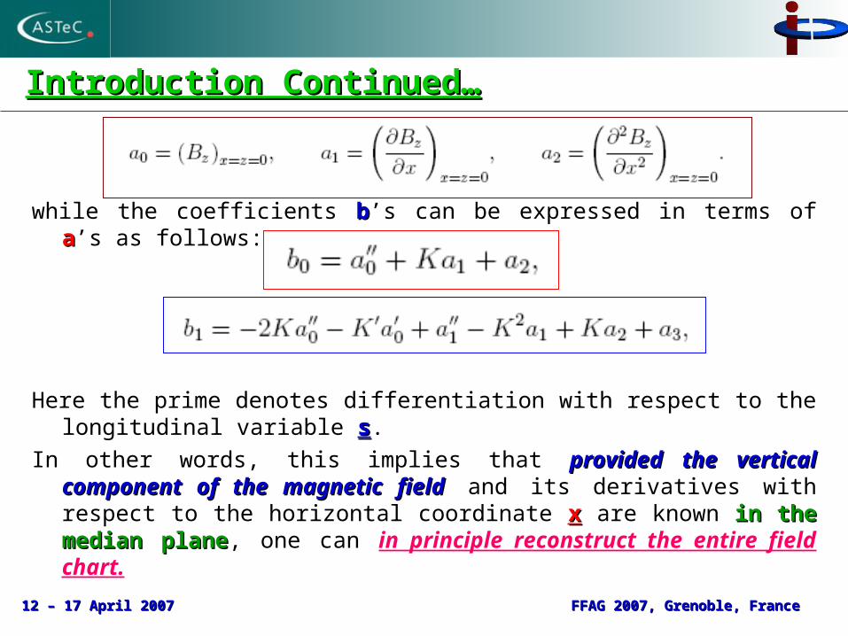
The coefficients aa's have a very simple meaning:


Introduction Continued…Introduction Continued…

while the coefficients bb’s can be expressed in terms of aa’s as follows:

Here the prime denotes differentiation with respect to the longitudinal variable ss.

In other words, this implies that provided the vertical component of the provided the vertical component of the magnetic fieldmagnetic field and its derivatives with respect to the horizontal coordinate xx are known in the median planein the median plane, one can in principle reconstruct the entire field chart.


The Synchro-Betatron Formalism and the Reference OrbitThe Synchro-Betatron Formalism and the Reference Orbit

The vertical component of the magnetic field in the median planevertical component of the magnetic field in the median plane of the machine can be expressed as

where

The flutter functionflutter function is periodic in the azimuthal variable, so that it can be expanded in a Fourier series:


The Synchro-Betatron Formalism Continued…The Synchro-Betatron Formalism Continued…

Let us introduce the relative variation of the vertical component of the magnetic field relative variation of the vertical component of the magnetic field in the median plane under deviationin the median plane under deviation from a fixed radius RR

Here we have denoted



In the case of In the case of NN-fold symmetry, the -fold symmetry, the flutter functionflutter function consists of a consists of a structural partstructural part including harmonics of the type including harmonics of the type n = kNn = kN and the rest ( and the rest (a non structural parta non structural part), ), which is usually which is usually considered as a perturbationconsidered as a perturbation. .

Let us now write the first several coefficients Let us now write the first several coefficients aa’s’s

A A design (reference) orbitdesign (reference) orbit with a with a reference momentum and reference angular reference momentum and reference angular velocityvelocity is defined according to the relation is defined according to the relation

FFAG 2007, Grenoble, FranceFFAG 2007, Grenoble, France12 – 17 April 200712 – 17 April 2007



Using the Using the explicit form of the mean field and the fact that it is a linear function in explicit form of the mean field and the fact that it is a linear function in radiusradius (in the case of EMMA), we obtain (in the case of EMMA), we obtain

where for brevity we have denotedwhere for brevity we have denoted

Typical rangeTypical range of angular velocity is from of angular velocity is from 1.9422 GHz – 995.3 MHz1.9422 GHz – 995.3 MHz for energies in for energies in the range the range 10 MeV – 20 MeV10 MeV – 20 MeV, respectively. In terms of the , respectively. In terms of the azimuthal variable as azimuthal variable as an independent variablean independent variable, we can rewrite the Hamiltonian as follows, we can rewrite the Hamiltonian as follows


Here we have introduced the following notations:

The reference orbit reference orbit can be defined via a canonical transformation



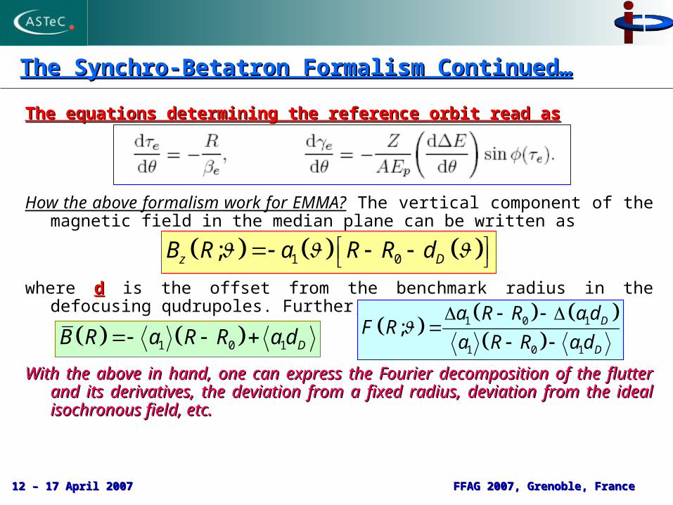
The equations determining the reference orbit read asThe equations determining the reference orbit read as

How the above formalism work for EMMA? The vertical component of the magnetic field in the median plane can be written as

where dd is the offset from the benchmark radius in the defocusing qudrupoles. Further,

With the above in hand, one can express the Fourier decomposition of the flutter With the above in hand, one can express the Fourier decomposition of the flutter and its derivatives, the deviation from a fixed radius, deviation from the ideal and its derivatives, the deviation from a fixed radius, deviation from the ideal isochronous field, etc. isochronous field, etc.

1 0;z DB R a R R d


1 0 1 DB R a R R a d

1 0 1

1 0 1

; D

D

a R R a dF R

a R R a d

Accelerated Orbit and DispersionAccelerated Orbit and Dispersion

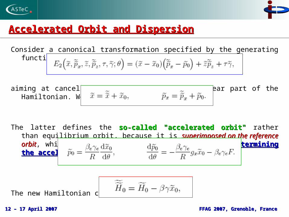
Consider a canonical transformation specified by the generating function

aiming at cancelling the first term in the linear part of the Hamiltonian. We have

The latter defines the so-called "accelerated orbit"so-called "accelerated orbit" rather than equilibrium orbit, because it is superimposed on the reference orbitsuperimposed on the reference orbit, which is NOT a closed curveNOT a closed curve. The equations determining the accelerated orbit areThe equations determining the accelerated orbit are

The new Hamiltonian can be written as


Accelerated Orbit and Dispersion Continued…Accelerated Orbit and Dispersion Continued…

Taking into account additionally the reference orbitreference orbit, and assuming that the deviation of the energy with respect to the reference one is small, we can cast the above Hamiltonian in the form


Accelerated Orbit and Dispersion Continued…Accelerated Orbit and Dispersion Continued…

The last canonical transformation aimed at cancelling the linear part of the cancelling the linear part of the Hamiltonian isHamiltonian is

Taking into account that the dispersion function D D satisfies the set of equations

the new Hamiltonian can be expressed as


The Betatron Motion and Twiss ParametersThe Betatron Motion and Twiss Parameters

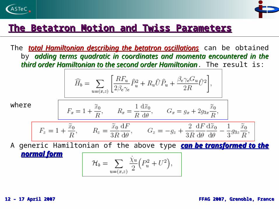
The total Hamiltonian describing the betatron oscillationstotal Hamiltonian describing the betatron oscillations can be obtained by adding adding terms quadratic in coordinates and momenta encountered in the third order terms quadratic in coordinates and momenta encountered in the third order Hamiltonian to the second order HamiltonianHamiltonian to the second order Hamiltonian. The result is:

where

A generic Hamiltonian of the above type can be transformed to the normal formcan be transformed to the normal form


The Betatron Motion and Twiss Parameters Continued…The Betatron Motion and Twiss Parameters Continued…

by means of a canonical transformation specified by the generating function:

The old and the new canonical variables are related through the expressions

The phase advance and the generalized Twiss parametersadvance and the generalized Twiss parameters are defined as

The corresponding betatron tunescorresponding betatron tunes are determined according to the expression


The Reference Orbit and AccelerationThe Reference Orbit and Acceleration

We will solve explicitly the equations determining the accelerated orbitequations determining the accelerated orbit in the case where the accelerating force exerted by the cavities is considered in the in the kick approximationkick approximation. We can write

Here is the cavity voltage, is the RF frequency, NcNc is the number of cavities and is the corresponding cavity phase. We introduce a new variable

It is straightforward to write the transfer maptransfer map for the interval just before entering the k-thk-th cavity to the location just before entering the (k+1)-st(k+1)-st cavity. It has the form


The Reference Orbit and Acceleration Continued…The Reference Orbit and Acceleration Continued…

The reference orbit map is a generalized Standard Map,generalized Standard Map, which is known to exhibit the so-called accelerator modesaccelerator modes. To find the accelerator modes, we expand the relevant variables in a formal small parameterrelevant variables in a formal small parameter according to the relations:

Order by order one finds:

Performing further analysis, one can find the amplitude equationamplitude equation governing the nonlinear acceleration regimenonlinear acceleration regime. It is of the form:

Highly nontrivial problemHighly nontrivial problem, which is now in progress.

20 0 1 2...e


20 1 2 ...e e e eT T T T

0eT 0 B const

1

1 1

sinsin 2

4

cNkRF

k kk mp

mZeU

AE m

2 ...c c c

dBB B

d

The Phase MotionThe Phase Motion

Clearly, the phase motionphase motion depends only on the horizontal degree of freedomhorizontal degree of freedom. The total Hamiltonian after extracting the accelerated orbitafter extracting the accelerated orbit can be written as

The equations of motion with account of the accelerated orbit only read as

A more rigorous treatment is achieved if the dispersion effectsdispersion effects are included in the analysis.

All these are now in progressare now in progress. It should be mentioned that the phase motion in FFAG accelerators is HIGHLY NONTRIVIAL.

2 2 2 20 ... sin

2e e

x e e x xp

Z d EH R x p x g x x p d

R AE d

#


02 2 2

0

R xd

d p

sin

p

d Z d E

d AE d

Conclusions and OutlookConclusions and Outlook

A close parallel between isochronous cyclotrons and FFAG A close parallel between isochronous cyclotrons and FFAG accelerators has been established. accelerators has been established.

The transversal motion in both machines is very similar and can be The transversal motion in both machines is very similar and can be studied from a unified point of view. studied from a unified point of view.

However, the longitudinal dynamics differs. While in isochronous However, the longitudinal dynamics differs. While in isochronous cyclotrons the source of phase motion is the deviation of the real cyclotrons the source of phase motion is the deviation of the real magnetic field from the isochronous one, in FFAG machines the phase magnetic field from the isochronous one, in FFAG machines the phase motion is an essential part of the dynamics. motion is an essential part of the dynamics.

A computer code A computer code FFEMMAGFFEMMAG to simulate the linear dynamics in FFAG to simulate the linear dynamics in FFAG machines is now under development. It will calculate the reference orbit machines is now under development. It will calculate the reference orbit of EMMA, the median plane footprint, the lattice functions and of EMMA, the median plane footprint, the lattice functions and dispersion.dispersion.

Future work also includes dynamic aperture module, resonance crossing part, as well as a module to simulate space charge effects, which have proven to be very essential in EMMA.


AcknowledgementsAcknowledgements

Bruno MuratoriBruno Muratori is acknowledged as a principal collaboratorprincipal collaborator in the development of the FFEMMAG computer code, as well as for his enthusiasm during the learning processenthusiasm during the learning process dedicated to the principles and operation of FFAG machines.

Special thanks for many illuminating and fruitfulmany illuminating and fruitful discussions are due to: Neil Bliss

Neil MarksNeil Marks

Susan SmithSusan Smith

James Jones James Jones


hamiltonian description of the dynamics of particles in non scaling ffag machines stephan i. tzenov...

Documents

france slide

median plane

relation ffag

synchrobetatron formalism

magnetic field xin

reference momentum

mean field

design reference orbit