hamiltonian approach to resonant transport regimes due to

Christopher Albert

Hamiltonian Theory of Resonant Transport Regimes in Tokamaks with Perturbed Axisymmetry

Monographic Series TU Graz Computation in Engineering and Science

Series Editors G. Brenn Institute of Fluid Mechanics and Heat Transfer G. A. Holzapfel Institute of Biomechanics W. von der Linden Institute of Theoretical and Computational Physics M. Schanz Institute of Applied Mechanics O. Steinbach Institute of Applied Mathematics

Monographic Series TU Graz Computation in Engineering and Science Volume 38

Christopher Albert _____________________________________________________ Hamiltonian Theory of Resonant Transport Regimes in Tokamaks with Perturbed Axisymmetry ______________________________________________________________ This work is based on the dissertation “Hamiltonian Approach to Resonant Transport Regimes due to Non-Axisymmetric Magnetic Perturbations in Tokamak Plasmas”, presented at Graz University of Technology, Institute of Theoretical and Computational Physics in 2017.

Supervision / Assessment:

Martin Heyn (Graz University of Technology)

Per Helander (University of Greifswald)

Cover photo Vier-Spezies-Rechenmaschine

by courtesy of the Gottfried Wilhelm Leibniz Bibliothek –

Niedersächsische Landesbibliothek Hannover

Cover layout Christina Fraueneder, TU Graz

Stefan Schleich, TU Graz

Print DATAFORM Media Ges.m.b.H.

© 2020 Verlag der Technischen Universität Graz

www.tugraz-verlag.at Print ISBN 978-3-85125-746-5 E-Book ISBN 978-3-85125-747-5 DOI 10.3217/978-3-85125-746-5

https://creativecommons.org/licenses/by-nc-nd/4.0/

Preface

This book is a revised version of the author’s dissertation (Albert, 2017). Resonanttransport regimes in non-axisymmetrically perturbed tokamaks are treated by theapplication of Hamiltonian perturbation theory in action-angle variables. The mainadvantages of this method are the independence from assumptions on geometrysuch as the large-aspect-ratio limit and its extensibility to non-linear regimes. Inthe context of this problem, weakly non-linear theory is applied to go beyond thequasilinear limit and allow for a physically consistent transition between limitingcases.

Naturally, a significant portion of this text is dedicated to the review of well-knownconcepts found in the cited literature and aims to clarify some details, which maynot be obvious to a graduate student studying the scientific literature, or not obviousat all. In that sense, the text is aimed to be useful for the reader to efficiently acquireknowledge on both, required basics and the specific topic.

The initial part introduces methods for studying resonant effects in a perturbedHamiltonian system subject to collisional effects. To separate the essential pointsfrom additional requirements in the general case, the development starts with abottom-up approach, where concepts are developed based on a one-dimensionalexample and then generalised to a wider class of systems. In the second part, theHamiltonian description of guiding-centre motion in an axisymmetric magnetic fieldis reviewed together with some required aspects of plasma kinetic theory. Finally,the general form of the method from the first part is applied to the specific problemof resonant transport regimes in a non-axisymmetrically perturbed tokamak plasma.

Results from computations confirm the significance of contributions from those re-gimes to neoclassical toroidal viscous torque in medium-sized tokamaks with mag-netic perturbations from coils installed for the control of edge-localized modes. Themajor features of this work appear to be relevant for quantitative evaluation of tor-oidal torque, namely complete geometry, consideration of magnetic drift, magneticshear and the transition region between quasilinear and non-linear regimes underthe assumption of well-separated resonances.

Acknowledgements

Working in the group of Martin Heyn and Winfried Kernbichler under the supervisionof the former has been a very rewarding experience that allowed me to explore afield of research that I have learned to love during the past years. I am especiallygrateful to Sergei Kasilov, whose unique physical intuition and countless hours spenttogether in Graz and Kharkov have been of priceless value both professionally andpersonally. For continuous professional and personal support in the office, I wouldlike to thank my colleagues Gernot Kapper and Andreas Martitsch. Furthermore, Iwould like to extend my gratitude to Ker-Chung Shaing and Wolfgang Suttrop fortheir continued interest in our group’s work and valuable discussions. As one canlearn a lot by teaching, I owe a great deal of insight to the students with whomI had the pleasure to work together, especially Lukas Grabenwarter, Patrick Lainer,Katharina Rath and Florian Seeber. To my parents Brigitte and Hans Albert, I amforever indebted for their guidance and the foundation that allowed me to pursuethis path. My greatest thanks go to my beloved Romana, who makes it possible forme to keep my balance between physics and real life.

This work has been carried out within the framework of the EUROfusion Consortiumand has received funding from the Euratom research and training programme 2014-2018 under grant agreement No 633053. The views and opinions expressed hereindo not necessarily reflect those of the European Commission. The author gratefully ac-knowledges support from NAWI Graz and funding from the KKKÖ at ÖAW for the initialpart of the work as well as the OeAD under the grant agreement “Wissenschaftlich-Technische Zusammenarbeit mit der Ukraine” No. UA 06/2015.

Contents

0 Introduction 7

1 Hamiltonian mechanics 131.1 Lagrangian, Hamiltonian and equations of motion . . . . . . . . . . . 131.2 Action-angle variables . . . . . . . . . . . . . . . . . . . . . . . . . . 161.3 A one-dimensional example . . . . . . . . . . . . . . . . . . . . . . . 171.4 Treatment of perturbations and resonances . . . . . . . . . . . . . . 231.5 Fourier harmonics in canonical angles . . . . . . . . . . . . . . . . . 281.6 A numerical experiment for the pendulum . . . . . . . . . . . . . . . 29

2 Kinetic description and resonant interaction 332.1 Liouville’s theorem . . . . . . . . . . . . . . . . . . . . . . . . . . . . 332.2 Collisions and the kinetic equation . . . . . . . . . . . . . . . . . . . 352.3 Weakly non-linear kinetic theory . . . . . . . . . . . . . . . . . . . . 372.4 Quasilinear limit . . . . . . . . . . . . . . . . . . . . . . . . . . . . . 402.5 Non-linear limit . . . . . . . . . . . . . . . . . . . . . . . . . . . . . . 432.6 Numerical solution for weakly non-linear kinetics . . . . . . . . . . . 46

3 Hamiltonian theory of guiding-centre motion in a tokamak 513.1 Guiding-centre Lagrangian . . . . . . . . . . . . . . . . . . . . . . . . 513.2 Canonical form of the guiding-centre Lagrangian . . . . . . . . . . . 533.3 Transformation of radial dependencies . . . . . . . . . . . . . . . . . 553.4 Action-angle variables in quasi-1D systems . . . . . . . . . . . . . . . 573.5 Action-angle variables in a tokamak . . . . . . . . . . . . . . . . . . . 633.6 Thin orbit approximation . . . . . . . . . . . . . . . . . . . . . . . . 673.7 Approximate transformation to canonical coordinates . . . . . . . . . 74

4 Resonant transport regimes 774.1 Basic kinetic theory . . . . . . . . . . . . . . . . . . . . . . . . . . . . 774.2 Kinetic equation and conservation laws . . . . . . . . . . . . . . . . . 794.3 Toroidal torque density and flux-force relation . . . . . . . . . . . . . 82

6 CONTENTS

4.4 Hamiltonian perturbation . . . . . . . . . . . . . . . . . . . . . . . . 834.5 Quasilinear approximation . . . . . . . . . . . . . . . . . . . . . . . . 854.6 Non-axisymmetric magnetic perturbation . . . . . . . . . . . . . . . . 884.7 Quasilinear resonant transport regimes and NTV torque . . . . . . . 894.8 Transport coefficients . . . . . . . . . . . . . . . . . . . . . . . . . . . 914.9 Transition to non-linear transport regimes . . . . . . . . . . . . . . . 93

5 Results and discussion 1015.1 Quasilinear resonant transport regimes . . . . . . . . . . . . . . . . . 1015.2 Non-linear resonant transport regimes . . . . . . . . . . . . . . . . . 1105.3 Treatment of finite orbit width . . . . . . . . . . . . . . . . . . . . . . 1125.4 Summary and Outlook . . . . . . . . . . . . . . . . . . . . . . . . . . 116

A Construction of magnetic flux coordinates 119A.1 Clebsch Form . . . . . . . . . . . . . . . . . . . . . . . . . . . . . . . 119A.2 Magnetic flux . . . . . . . . . . . . . . . . . . . . . . . . . . . . . . . 120A.3 Transformation to flux coordinates . . . . . . . . . . . . . . . . . . . 122

B Analytical comparison to existing results 123B.1 Toroidal drift frequencies . . . . . . . . . . . . . . . . . . . . . . . . 123B.2 Bounce integrals in the large-aspect-ratio limit . . . . . . . . . . . . . 124B.3 Eulerian approach to drift-orbit resonances . . . . . . . . . . . . . . . 126B.4 Transport coefficients for bounce-drift resonances . . . . . . . . . . . 131B.5 Expressions for the transit-drift resonance . . . . . . . . . . . . . . . 134

List of Figures 139

Bibliography 141

Introduction

Background

The general topic of this text is the behaviour of magnetically confined fusion plas-mas in tokamaks with small non-axisymmetric perturbations. For readers not fa-miliar with the issue this section will give a very short introduction together withreferences to relevant literature. A current overview can be found e.g. in the re-view articles of Boozer (2005) and Ongena et al. (2016). In the last paragraph, thepurpose of the present work in this general context is outlined.

Magnetic confinement fusion is considered to be a potential technology for sus-tainable world-wide large-scale energy supply. In analogy to the natural processesheating the Sun, fusion reactions between small nuclei are used as a power source.To initiate this process, the nuclei have to be brought together sufficiently close,which is possible by gravitational pressure inside the Sun. Here on earth, we haveto rely on other mechanisms, one of them being a magnetic trap for a sufficientlyhot plasma of nuclei (usually deuterium and tritium) together with their electrons.To produce a significant amount of energy by fusion reactions that allow for theplasma to be mostly self-heated (or fully – ignited), the product of density, pressureand energy confinement time has to be sufficiently high (Lawson, 1957). Devicescurrently believed to be able to fulfil those requirements1 are tokamak (Artsimovich,1972; Wesson, 2011), and stellarator (Spitzer, 1958). Both of these devices have thetopology of a torus and rely on magnetic coils to produce a toroidal magnetic field.In the stellarator, additional poloidal field components required for plasma stabilityare produced by a twisted coil geometry. The classical tokamak is an axisymmet-ric device, which means that toroidal currents are required to produce a poloidalmagnetic field. Up to today, the best confinement properties have been reached inso-called H-mode plasmas in tokamaks (Wagner et al., 1984), which has made itpossible to achieve fusion gains of the order of heating power already in the 1990s(Keilhacker et al., 1999). In this operational mode, a transport barrier is formed at

1Another possible candidate is inertial confinement fusion (Nuckolls and Wood, 1972), whichrelies on laser beams instead of magnetic fields, which is not the scope of the present text.

8 CONTENTS

the plasma edge, which results in a substantial enhancement of energy confinementtime. This improvement comes at a cost: the occurrence of edge-localised modesor ELMs (Zohm, 1996), small instabilities that lead to the continuous expulsion ofheat towards the device wall, is still an issue of active research. While not dramaticfor current devices, those modes will have to be reduced or suppressed in futuredevices of dimensions large enough for significant energy production, namely ITER(Loarte et al., 2003), to avoid damage to the wall. One way to achieve this purposeis to intentionally perturb the original axisymmetry by so-called resonant magneticperturbations or RMPs (Evans et al., 2004) using additional coils.

The purpose of this work is the investigation of side-effects from such perturba-tions on toroidal plasma rotation. One reason for the importance of this questionis the requirement of sufficiently high toroidal plasma rotation for magnetohydro-dynamic stability (Ida and Rice, 2014). In a completely axisymmetric plasma, thetoroidal rotation velocity can in principle take arbitrary values due to conservationof toroidal angular momentum linked to this symmetry. Breaking the symmetry bynon-axisymmetric magnetic field perturbations, e.g. by toroidal field ripple, errorfields or RMP fields, leads to non-ambipolar transport that results in toroidal rota-tion damping, an effect known as neoclassical toroidal viscous (NTV) torque (Shaing,1986; Shaing et al., 2010). Accurate computation of this effect is possible and re-quired for the distinction from turbulent effects not considered here (Kasilov et al.,2014; Martitsch et al., 2016).

It should be stressed that NTV torque is related to the part of the RMP field that is notin resonance with the equilibrium magnetic field, while the resonant part leads toadditional resonant torque, which requires a different treatment (Heyn et al., 2008).In this sense, the term resonant used here is not related to the “R” of RMP but ratherto orbital resonances, which can play a major role in NTV torque at low-collisionalityconditions relevant for reactor applications (Martitsch et al., 2016). Although initialresults from a fully numerical kinetic approach to the effect of RMPs in tokamaks(including resonant torque) have been published (Albert et al., 2016c), the scopeof this text is intentionally limited to the self-contained topic of the Hamiltonianapproach to resonant transport regimes of NTV torque.

The first task of this work is to formulate a method to treat the quasilinear limit(Romanov and Filippov, 1961; Vedenov et al., 1961) produced by infinitesimalperturbations without the limitations of bounce-averaging or expressions for largeaspect-ratios. This is done by a Hamiltonian approach in action-angle coordinatesintroduced by Taylor (1964) first for magnetic traps, established in the context ofquasilinear transport in tokamak plasmas by Kaufman (1972), and applied in par-ticular by Hazeltine et al. (1981) and Mahajan et al. (1983). A notable applicationof the Hamiltonian approach is plasma heating by quasilinear wave-particle inter-

CONTENTS 9

action (Osipenko and Shurygin, 1989, 1990; Bécoulet et al., 1991; Eriksson andHelander, 1994; Timofeev and Tokman, 1994; Kasilov et al., 1997). Since perturb-ation amplitudes can reach more than half a percent of the axisymmetric magneticfield module (Martitsch et al., 2016), the second task is to overcome the limita-tion of infinitesimal perturbations required for quasilinear theory. To achieve this,non-linear effects by orbital resonances are taken into account following secularperturbation theory (Chirikov 1960; 1979) in combination with a kinetic approachdescribing the transition between quasilinear and non-linear limit, where the lim-iting cases have originally been introduced in the context of plasma wave-particleinteraction (Romanov and Filippov, 1961; Vedenov et al., 1961; Zakharov and Karp-man, 1963).

10 CONTENTS

Overview

The main features of this work are the following:

• Unified descriptions of low-collisional quasilinear and non-linear resonant trans-port regimes of neoclassical viscous torque in non-axisymmetrically perturbedtokamak plasmas without limitations on device geometry.

• Accurate transition between superbanana and superbanana plateau regimesand equivalent bounce resonance regimes.

• Review of the construction of action-angle coordinates and canonical frequen-cies in a tokamak.

• Natural appearance of a magnetic shear term that is absent in the standardlocal neoclassical ansatz.

• Extension to consider the full orbit width for computation of toroidal torque.

• Demonstration that a momentum-conserving collision operator is not requiredfor quasilinear resonant transport regimes at sub-sonic rotation.

• Illustration of importance of the discovered features on a model tokamak andASDEX Upgrade with resonant magnetic perturbations.

• Efficient implementation in the code NEO-RT (Albert and Kasilov, 2017) byinterpolation of pre-computed frequencies and a non-linear attenuation para-meter.

This first chapter on Hamiltonian mechanics should serve as a quick overview ofwell-known concepts and methods that are applied in the subsequent chapters. Inparticular, this includes the treatment of resonances in the context of Hamiltonianperturbation theory, which is demonstrated on the example of a one-dimensionalpendulum. Moreover, a number of notations and conventions used in the remainingtext will be defined here. In chapter 2 the basic concepts of kinetic theory are out-lined and the general weakly non-linear perturbation theory in the low-collisionalitylimit is introduced.

Chapter 3 describes the transformation to action-angle variables for the guiding-centre motion of in the magnetic field of a tokamak. Though the use of actionsand adiabatic invariants dates back to the beginning of research in the field of mag-netic plasma confinement, some specific details needed for a consistent derivationare not completely clear from common literature. One of these peculiarities is thetransformation of geometrical angles from magnetic coordinates in a way to obtain

CONTENTS 11

a canonical form of the guiding-centre Lagrangian. This has been solved by an exacttransformation closely related to the one of Li et al. (2016) and additionally by amodification of the approximate method of White (1990).

In chapter 4, general conservation laws for flux-surface averaged quantities are for-mulated with emphasis on particle density and toroidal momentum density. Thetoroidal torque at low collisionality due to a small non-axisymmetric Hamiltonianperturbation is derived based on the action-angle variables for the unperturbed sys-tem for the quasilinear case. The approach is then extended to the weakly non-linearcase (lower collisionality and/or higher perturbation amplitudes), where new orbitclasses (e.g. superbananas) become relevant.

In chapter 5 results from computations from the code NEO-RT (Albert and Kasilov,2017) that has been developed based on the presented approach are presented, val-idated and analysed. Computations have been performed for test cases in a circulartokamak and equilibria from the experiment ASDEX Upgrade with ELM control coils(resonant magnetic perturbations or RMPs). In the end, an outlook on the possibletreatment of finite orbit width is given. The chapter is mostly based on parts of theauthor’s publications on the topic to which references are given.

Finally, the appendix includes details on the construction of magnetic flux coordin-ates, analytical comparisons to existing works and a list of formulas used in deriva-tion and implementation of the method.

Some remarks on the notation

To balance clarity and readability, dependent variables of functions are given expli-citly where needed, e.g. in the first occurrence of partial derivatives ∂J‖(J⊥, H, pϕ)/∂pϕ

and omitted in subsequent lines as in ∂J‖/∂pϕ. Jacobians of variable transforma-tions (x1, x2, x3)→ (y1, y2, y3) are denoted by

∂(x1, x2, x3)

∂(y1, y2, y3)≡ det

∂x1(y1,y2,y3)

∂y1

∂x1(y1,y2,y3)∂y2

∂x1(y1,y2,y3)∂y3

∂x2(y1,y2,y3)∂y1

∂x2(y1,y2,y3)∂y2

∂x2(y1,y2,y3)∂y3

∂x3(y1,y2,y3)∂y1

∂x3(y1,y2,y3)∂y2

∂x3(y1,y2,y3)∂y3

. (1)

N-tuples of quantities (this includes vectors) are denoted by bold-face letters, i.e.J = (J1, J2, J3). In particular for vectors, the co- and contravariant notation withsuperscripts and subscripts (see, e.g. the book of D’haeseleer et al. (1991)) is chosen.The sum convention applies for repeated indices at opposite positions,

akbk ≡∑k

akbk. (2)

There are a few ambiguities in the notation, most notably the use of letters m andn for both mass/density as well as harmonic indices, and the use of Dij not only

12 CONTENTS

as components of diffusivity but also as transport coefficients later. Normally, thechoice should be clear from the context, and otherwise the notation is resolved byadditional comments and/or by including subscript α for the particle species, i.e.mα is the mass of species α.

Chapter 1

Hamiltonian mechanics

1.1 Lagrangian, Hamiltonian and equations of motion

A classical mechanical system (see e.g. the books of Goldstein (1980), Landau andLifshitz (1960), Lichtenberg and Lieberman (1983) or Arnold (1989)) is fully char-acterised by its Lagrangian L(q, q, t), which is a function of N generalised coordin-ates qi in configuration space, N generalised velocities qi and time t. The solution ofa mechanical problem is given by a trajectory in configuration space, i.e. a twicecontinuously differentiable curve q(t) for which q(t) = dq(t)/dt, and the actionfunctional

S =

t1

t0

dt L(q(t), q(t), t) (1.1)

takes an extremal value. Here, in contrast to many other texts, we did not identifydotted notation with a time derivative a priori – the three quantities q, q(t) anddq(t)/dt are of different nature. Without argument, q describes N independentvelocity variables, q(t) their evolution over time parameter t, and dq(t)/dt a tangentvector to the parameterized curve q(t) in configuration space. Only in Lagrangianmechanics one immediately identifies q(t) with the curve velocity dq(t)/dt alreadyat the level of the action law, thereby effectively dropping N velocity dimensionsto work only in N -dimensional configuration space. In that case one can deducethat each component of q(t) must fulfil a set of N second-order ordinary differentialequations – the Euler-Lagrange equations

d

dt

(∂L

∂qi(q(t), q(t), t)

)− ∂L

∂qi(q(t), q(t), t) = 0. (1.2)

Here, at first, qi and qi are treated as independent variables in 2N -dimensional (velo-city) phase-space on which L(q, q, t) is defined. Only after taking partial derivatives,one may set q ≡ q(t) and q ≡ q(t) = dq(t)/dt to their values along the trajectoryand take a total time derivative.

14 CHAPTER 1. HAMILTONIAN MECHANICS

Since the extremal path in Eq. (1.1) is not affected by a constant shift in S, adding atotal time derivative inside the integral results in a new Lagrangian

L(q(t), q(t), t) = L(q(t), q(t), t) +dF (q(t), q(t), t)

dt, (1.3)

that describes the same mechanical system as L. Here, F can be any dynamicalvariable (a function depending on position, velocity and time), for which the totaltime derivative is defined as

dF (q(t), q(t), t)

dt=∂F

∂t+

dqi(t)

dt

∂F

∂qi+

dqi(t)

dt

∂F

∂qi

=∂F

∂t+ qi(t)

∂F

∂qi+

dqi(t)

dt

∂F

∂qi(1.4)

along any trajectory. If all ∂F/∂qi vanish one may describe such a total time deriv-ative as

dF (q(t), t)

dt=

DF

Dt(q(t), q(t), t), (1.5)

whereDF

Dt(q, q, t) =

∂F (q, t)

∂t+ q · ∂F (q, t)

∂q, (1.6)

is an advective derivative being a function on positions, velocities and time, inde-pendent from the actual trajectory. The latter is only inserted in Eq. (1.5).

Derivatives of L with respect to qi are called generalised momenta

pi =∂L(q, q, t)

∂qi, (1.7)

which are conserved along any actual trajectory q(t) (short: conserved), in case L isindependent of the respective coordinate qi. Together with q, canonical momentap form a set of so-called canonically conjugate coordinates in 2N -dimensional phasespace. Introducing the Hamiltonian H(q,p, t) by a Legendre transformation

H(q,p, t) = p · q(q,p)− L(q, q(q,p), t),

we obtain the equivalent Hamiltonian description of Eq. (1.2). Here yet another useof the velocity symbol is introduced, with q(q,p) being velocity components of acoordinate transformation from canonical coordinates (q,p) to non-canonical phase-space coordinates (q, q).1 The resulting set of 2N first-order ordinary differentialequations,

dqi(t)

dt=∂H

∂pi(q(t),p(t), t),

dpi(t)

dt= −∂H

∂qi(q(t),p(t), t), (1.8)

1This also clarifies that the term “velocity phase-space” is a result of (incorrectly) identifying co-ordinates with the actual space – there is only one phase-space where phase-points can be describedby different systems of coordinate.

1.1. LAGRANGIAN, HAMILTONIAN AND EQUATIONS OF MOTION 15

describes the temporal evolution of coordinates and momenta. They are calledHamilton’s equations of motion or canonical equations. This formulation is a geo-metrical one, as the right-hand side of Eqs. (1.8) describes a so-called Hamiltonianvector field (

q

p

)=

(∂H/∂p

−∂H/∂q

)=

(0 I

−I 0

)∇q,pH, (1.9)

and the left-hand side its integral curves. Similar to the Lagrangian formalism above,we will only identify the (global) vector field of phase-velocities q and p with the(local) tangent to a particular orbit q(t) and p(t) if explicitly stated as q(t), p(t).

Introducing the Poisson bracket

f, g ≡ ∂f

∂qi∂g

∂pi− ∂f

∂pi

∂g

∂qi, (1.10)

total time derivatives of dynamical variables f(q,p, t) along a phase-trajectory isexpressed by

df(q(t),p(t), t)

dt=∂f

∂t+

dqi(t)

dt

∂f

∂qi+

dpi(t)

dt

∂f

∂pi=∂f

∂t+ f,H, (1.11)

with the right-hand side evaluated at (q(t),p(t), t). In the Hamiltonian formal-ism, it becomes thus particularily easy to write an advective derivative of f alongthe Hamiltonian (phase-velocity) vector field (1.9) along phase-space trajectories.Namely,

Df

Dt(q,p, t) =

∂f

∂t+∂H

∂pi

∂f

∂qi− ∂H

∂qi∂f

∂pi=∂f

∂t+ f,H, (1.12)

and for a particular trajectory

df(q(t),p(t), t)

dt=

Df

Dt(q(t),p(t), t). (1.13)

This will allow us to use df/dt and Df/Dt synonymously, as long as a relation isvalid for all trajectories defined by H. This is in contrast to Eq. (1.4) of the Lag-rangian formalism, where dq(t)/dt would first have to be expressed via the Euler-Lagrange equations (1.2) to obtain an equivalent expression.

For q and p, canonical equations (1.8) may also be written as

dqi(t)

dt= qi, H,

dpi(t)

dt= pi, H. (1.14)

For the Hamiltonian itself, it follows that

dH

dt=∂H

∂t=∂L

∂t. (1.15)


Hence, if L(q, q, t) = L(q, q) does not explicitly depend on time, H is conservedalong the trajectories defined via L. If there are no explicitly time-dependent con-straints in addition, H is equal to the total energy. We call such systems conservative.

It is possible to switch to a new set of canonically conjugate variables (q, p) bycanonical transformations that leave the Poisson brackets (1.10) invariant,

f, g =∂f

∂qi∂g

∂pi− ∂f

∂pi

∂g

∂qi. (1.16)

This is usually performed via a generating function, for example F2 = F2(q, p, t) and

pi =∂F2

∂qi, qi =

∂F2

∂pi. (1.17)

If F2 depends on time explicitly, H is transformed to a new Hamiltonian2

H(q, p) = H +∂F2

∂t. (1.18)

1.2 Action-angle variables

A conservative system is called integrable if it is possible to find a set of N independ-ent first integrals of motion α with dα/dt = 0 and αi, αj = 0. A specific set of αuniquely determines the trajectory in phase space together with N initial values. Ifthe motion is bounded in phase space, it can then be shown (see e.g. Arnold (1989))to be conditionally periodic, i.e., it is possible to choose angle variables θ that evolvelinearly in time for any trajectory, so

θ(t) = Ωt, (1.19)

with conserved canonical frequencies Ω = Ω(α). The pairs (θ,α) do not generallyform a set of canonically conjugate coordinates. It is however possible to perform atransformation J(α) to a set of N action variables J that are canonically conjugateto the angles θ. One also says thatα are a set of coordinates inN -dimensional actionspace. Conversely, α = α(J) can be written as functions of canonical actions. Inparticular, since H = α1 itself is conserved, it will depend only on J but not on θ.From Eq. (1.8) we obtain

dJi(t)

dt= 0, (1.20)

dθi(t)

dt= Ωi =

∂H(J)

∂Ji. (1.21)

2Sometimes called the Kamiltonian due to its often used label K (Goldstein, 1980, p. 380)

1.3. A ONE-DIMENSIONAL EXAMPLE 17

To determine action-angle variables for a certain system, a canonical transforma-tion (q,p) → (θ,J) is performed via the abbreviated action (also called Hamilton’scharacteristic function) written in terms of q and α,

W (q,α) =

q

q0

dq′ · p(q′,α) (1.22)

=

ζ1

ζ0

dζdqi(ζ)

dζpi(q(ζ),α), (1.23)

where the integral is taken along a path of constant α, which also implies constantJ . This path is the actual trajectory in phase space for this specific set of α. Never-theless, the curve parameter ζ used for integration can be different from time t.

The transformation reads

pi(q,J) =∂W (q,α(J))

∂qi, (1.24)

θi(q,J) =∂W (q,α(J))

∂Ji=

(∂J

∂α

)−1 ∂W (q,α)

∂α. (1.25)

The actions can be easily computed explicitly in the case of a separable system, wherefor a certain set of (q,p), W can be written as a sum of terms depending only onone coordinate each,

W (q,α) =∑i

Wi(qi,α) =

dqi pi(q

i,α) . (1.26)

In a separable system, the actions are given by integrals

Ji(α) =1

2π

dqi pi(q

i,α) =1

2π

dqi

∂Wi(qi,α)

∂qi(1.27)

taken either over the range of motion of one round-trip (back and forth) if oscillatory(libration) or one period in qi if periodic (rotation). We will keep this distinctionin mind to maintain consistent sign conventions for canonical actions, angles andfrequencies later.

Finally we note that in action-angle variables dynamical time derivatives in Eq. (1.11)take an especially simple form using Poisson brackets with the Hamiltonian,

f,H = Ωi ∂f

∂θi. (1.28)

1.3 A one-dimensional example

To illustrate the methods that are defined in a general way, let us consider a conser-vative one-dimensional mechanical system of a particle with mass mα, position x,momentum p in a potential U(x). The Hamiltonian of such a system is given by


H =p2

2mα+ U(x) (1.29)

and the equations of motion are

dx

dt=

p

mα, (1.30)

dp

dt= −dU(x)

dx. (1.31)

Because H is conserved in this system, it can be used to write p as a function ofposition and integrals of motion,

p(x,H) = σ√

2mα(H − U(x)), (1.32)

∂p(x,H)

∂H= σ

√mα

2

1√H − U(x)

=mα

p(x,H). (1.33)

The constant σ = ±1 specifies whether the motion is directed towards the positiveor negative x direction. Since the system is one-dimensional, the abbreviated actionW in Eq. (1.26) is trivially separable, since it contains only one term

W = Wx =

x

x0

dx′ p(x,H)

=

x

x0

dx′ σ√

2mα(H − U(x)). (1.34)

To be more specific, let us choose a cosine-shaped potential

U(x) = U0(1− cos(x))

= 2U0 sin2(x/2), (1.35)

which results in the Hamiltonian

H =p2

2mα+ U0(1− cos(x)). (1.36)

The classical physical interpretation of this system is the pendulum of mass mα ona rigid, massless rod in a homogeneous gravitational field. In this case, x takes therole of the angle of the pendulum towards the vertical axis. Alternatively, it canrepresent a particle in a 2π-periodic cosine-shaped potential well. In that case, x isinterpreted as a Cartesian coordinate and the size of the system is infinite. In a moreabstract sense, this Hamiltonian also appears in weakly non-linear approximations


within more complex systems, which will become clear in the subsequent section.Integrals of the type (1.34) for the pendulum Hamiltonian can be represented byelliptic integrals E and K depending on the parameter

κ = k2 ≡ H

2U0,

defined e.g. in the book of Gradshtein and Ryzhik (1965) (see also the article ofBrizard (2013), who uses the same notation for elliptic integrals as we do here).

One important feature of the pendulum Hamiltonian is the existence of two distincttypes of motion. If the parameter κ is smaller than one, the libration kind of motionis bounded between two turning points given by

H = U(x±) = U0(1− cos(x±)) , (1.37)

x± = ± arccos(1− 2κ) (1.38)

= ±2 arcsin(√κ). (1.39)

The classical pendulum would oscillate between those two points. For κ > 1, therotation kind of motion is unbounded, corresponding to a pendulum rotating overthe top. This kind of behaviour leads to two regions in phase space that have to betreated separately. The boundary in-between defined by κ = 1 is called separatrix.

To be consistent with later terminology, we switch to the particle-in-well interpreta-tion and call the librating orbits trapped and the rotating orbits passing.

For trapped orbits, the action associated to x is given by an integration forth andback between the turning points from Eq. (1.27),

J(H) =1

2π

x+

x−dx p(x,H)|σ=1 +

1

2π

x−

x+

dx p(x,H)|σ=−1

=1

π

x+

x−dx p(x,H)|σ=1

=1

π

x+

x−dx

√2mα(H − 2U0 sin2(x/2))

=

√2mαU0

π

x+

x−dx

√κ− sin2(x/2)

=√mαU0

8

π(E(κ)− (1− κ)K(κ)) . (1.40)

As mentioned at the end of section 1.2, the integration direction has been switchedat the turning points to result in a non-zero J .


For passing orbits, integration over one period of the motion in x results in

J(H) =1

2π

π

−πdx p(x,H)

= σ

√2mαU0

2π

π

−πdx

√κ− sin2(x/2)

= σ√mαU0

4√κ

πE(κ−1) . (1.41)

In contrast to the trapped case, we have maintained the positive x-direction in theintegration. The result are different signs in J distinguishing co-passing orbits withσ = 1 from counter-passing orbits with σ = −1. This detail of the sign conventionfor canonical actions is frequently neglected or taken for granted in the literature(it is for example clear that gyration of a positively charged particle in the negativesense results in negative magnetic moment). In any case we should keep it in mindfor the later developments for axisymmetric plasmas, where it will be crucial for thecorrect expressions for canonical variables.

The associated canonical frequency for trapped orbits is computed according to Eq.(1.21). For reasons that will become clear in the following paragraphs, we call it thebounce frequency ωb corresponding to the bounce time τb and write

Ω =

(∂J(H)

∂H

)−1

≡ ωb =2π

τb. (1.42)

Here, the derivative with respect to H in principle affects also the boundaries x± =

x±(H) by the Leibniz rule,

∂

∂H

x+(H)

x−(H)dx p(x,H) =

x+(H)

x−(H)dx

∂p(x,H)

∂H

+dx+(H)

dHp(x+, H)− dx−(H)

dHp(x−, H) . (1.43)

However, since p(x+, H) = p(x−, H) = 0 , the latter two boundary terms vanish andwe obtain

τb = 2πdJ

dH= 2

x+

x−dx

∂p(x,H)

∂H

∣∣∣∣σ=1

=√

2mα

x+

x−

dx√H − U(x)

=

√mα

U0

x+

x−

dx√κ− sin2(x/2)

. (1.44)

If the analytical solution for J were not known, one could integrate the equationsof motion ((1.30)-(1.30)) numerically and use the orbit time τ as an integrand to


substitute x, taking x(τ) from the orbit integration and

dx =p

mαdτ =

√2

mα

√H − U(x) dτ . (1.45)

The general bounce time integral (1.44) then becomes

τb =√

2mα

τ+

τ−

dτ√H − U(x(τ))

√2

mα

√H − U(x(τ))

= 2

τ+

τ−dτ , (1.46)

which is two times the time of one half-turn. As expected, this is indeed the bouncetime of the one-dimensional oscillation.

For our cosine potential in particular, we can just take a derivative of the analyticalsolution for the action in Eq. (1.40) and obtain

τb =

√mα

U04K (κ) , (1.47)

Ω =

√U0

mα

π

2K (κ)= ωb . (1.48)

The canonical frequency Ω is the bounce frequency ωb, which becomes the usualharmonic frequency

ω0 =

√U0

mα(1.49)

for κ 1 where the orbit remains close to x = 2nπ with integer n. Orbits atκ . 1 take longer and longer time to complete as the anharmonic contributions growstronger at higher energy (Fig. 1.1). At the separatrix κ = 1 the system approachesone of the unstable equilibrium points x = (2n + 1)π to come arbitrarily close withtime.

The bounce (transit) time for passing orbits can be computed by the same means.The analytical results for the cosine potential follow as

τb =

√mα

U0

2K(κ−1

)√κ

, (1.50)

Ω = σ

√U0

mα

π√κ

K (κ−1). (1.51)

This is already known as the canonical (bounce) frequency Ω = ωb, which cannow become negative for counter-passing particles, where σ = −1 over the whole


−1 0 1

x(t)/π

−2

−1

0

1

2

p(t

)

0.0 0.5 1.0 1.5 2.0

κ

0.0

0.5

1.0

1.5

2.0

ωb(κ

)/ω

0Figure 1.1: Left: pendulum orbits in phase-space with initial conditions equallyspaced in κ ∈ (0.05, 1.1585) traced until the bounce time τ0 = 2π/ω0 of the harmoniclimit at κ = 0 (solid) and their full shape (dashed). Right: dependency of bouncefrequency |ωb| on κ with limit 0 at the separatrix κ = 1. The frequency ωb of passingorbits becomes larger than ω0 already close to the separatrix, tending towards thelinear behaviour of free orbits further outside.

orbit. This follows from the sign convention when computing canonical angles formomenta from Eq. (1.25), which yields

θ(x, J) =

(∂J

∂H

)−1 ∂W (x,H)

∂H= Ω

∂W (x,H)

∂H. (1.52)

Using Eqs. (1.33) and (1.45), the canonical angle follows as

θ = Ω∂

∂H

x

x0

dx′ p(x,H) = Ω

x

x0

dx′∂p(x,H)

∂H

= Ω

τ

0dτ ′

p

mα

mα

p= τΩ = 2πσ

τ

τb, (1.53)

where the global σ = −1 is relevant for counter-passing orbits only. It is thus equalto the orbit time τ normalized to the bounce time τb (both always positive) span-ning 2π in one full turn and is valid for both, trapped and passing orbits in generalone-dimensional Hamiltonian systems. Here, the orbit time τ appears as a purelygeometrical quantity in phase space – a rescaled canonical angle θ. For the cosinepotential, it is given by the incomplete elliptic integral

θ(x) =πF(x2 |κ−1

)K(κ−1)

, (1.54)

in the passing region and by

θ(x) =πF(x2 |κ)

2K(κ)(1.55)

1.4. TREATMENT OF PERTURBATIONS AND RESONANCES 23

Figure 1.2: Evenly spaced contours of constant canonical actions J (left) and anglesθ (right) for the pendulum. By convention, J > 0 in the trapped region and hassign σ of p in the respective passing region. Angle θ is zero at x = 0 (in the trappedregion only for σ = 1) and grows with x in both passing regions specified by σ = ±1.

in the trapped region during the first half-oscillation x− < x < x+ with σ = +1,together with a phase-shifted variant of the expression for the other with σ = −1

(see Fig. 1.2).

For a general potential U(x) with local minima, multiple classes of trapped particleswith different turning points can arise, as long as their total energy H is below therespective local maximum that marks the boundary of the potential well. In thatcase, different starting positions x0 lead to different classes of canonical frequenciesand angles.

1.4 Treatment of perturbations and resonances

We are now going to introduce a time-harmonic perturbation H1(θ,J , t) on anoriginally unperturbed Hamiltonian H0(J) with the new Hamiltonian being H =

H0 +H1. The perturbation shall be of smaller order than H0 and be represented bya Fourier series

H1(θ,J , t) =∑m

Hm(J)ei(m·θ−ωt) (1.56)

with complex coefficients Hm. In case of a resonance

m ·Ω− ω = 0 (1.57)

between canonical frequencies Ω and perturbation frequency ω (which can also bezero), special treatment is required. The technique of choice is known as secularperturbation theory (Lichtenberg and Lieberman, 1983, p. 109) and can be appliedin a number of systems involving resonant interaction of a perturbation with the


original system. A review of the method with emphasis on resonance overlap andresulting Arnol’d diffusion is given by Chirikov (1979), who introduced the conceptof chaotic diffusion in his work on magnetic traps (Chirikov, 1960).

The applicability of the method relies on the resonances to be well separated, sowe can treat each harmonic m in canonical angles individually similar to the caseof a linear system. Still, the result is a 1-dimensional non-linear system for eachharmonic. This way, some non-linear features of the overall system are captured,which is the reason why the method can be classified as weakly non-linear. As wewill see, new orbit classes oscillating at a non-linear bounce frequency ωbN aroundeach resonance will emerge.

First, we introduce the resonant phase by a Galilean transformation

θ = m · θ − ωt+ θ0, (1.58)

where θ0 is defined to shift the complex phase of Hm such that

Hmei(m·θ−ωt) = −|Hm| cos θ . (1.59)

In the one-dimensional case with only one pair (θ, J), where the canonical angle isthe normalised bounce time of the unperturbed system, Eq. (1.58) can be written as

θ = mωbτ − ωt+ θ0, (1.60)

with a scalar harmonic index m. At the resonance condition (1.57) with ω = mωb,fulfiled only for a specific J = Jres, the interpretation of θ becomes clear from themodified expression

θ = ω(τ − t) + θ0. (1.61)

The physical meaning of θ is the normalised shift τ = θ/ω = τ − t + τ0 betweenthe orbit time τ of the unperturbed trajectory and the actual time in the perturbedsystem. Intuitively, this shift will develop faster with larger perturbation amplitudes.As we will see, the dynamics of θ close to the resonance condition can be modelledby a “super”-pendulum Hamiltonian with a non-linear (super)bounce frequenciesωbN . To allow for a perturbative treatment in this way, the time-scale of this newkind of motion should be much longer than the bounce time τ . The task of thefurther derivation is to find quantitative expressions to describe this behaviour.

For the 1D case, a canonical transformation replacing θ by θ together with its reson-ant action J is produced by the type-2 generating function

F2(θ, J) = J θ(θ)

= J (mθ − ωt− θ0). (1.62)


The original action J is related to J by

J =∂F2

∂θ= mJ. (1.63)

Specifically for non-zero ω, the explicit time dependence in F2 enters the unper-turbed Kamiltonian (1.18) given by

H0(J) = H0 +∂F2

∂t= H0 − ωJ . (1.64)

The new canonical frequency Ω is

Ω =∂

∂J(H0(J)− ωJ) =

∂J

∂J

∂H0(J)

∂J− ω = mΩ− ω. (1.65)

This expression vanishes at the 1D resonance condition (1.57), which is the intendedresult of our choice of the canonical transformation.

In the N -dimensional case the situation is similar. In contrast to the 1D case, wenow choose a specific action, e.g. JN (without loss of generality), to be replaced bythe resonant action J = JN . This approach is similar to the one of Bécoulet et al.(1991), where a general description in the direction perpendicular to the resonanceis used. A canonical transformation replacing a single angular coordinate by θ isproduced by the type-2 generating function

F2(θ, J) =∑k 6=N

Jkθk + J θ(θ)

=∑k 6=N

Jkθk + J (m · θ − ωt− θ0) . (1.66)

In this transformation, the new resonant phase θ = θN is defined as in Eq. 1.58, butall other angles stay the same with

θN = θ = m · θ − ωt− θ0, (1.67)

θk 6=N =∂F2

∂Jk= θk. (1.68)

The action JN is related to the resonant action J as in Eq. (1.63) via

JN = mN J , (1.69)

and the remaining original actions are modified via the components of their respect-ive component in the mode-number vector,

Jk 6=N =∂F2

∂θk= Jk +mkJ . (1.70)


This yields the transformed actions in terms of the original actions as

JN = J =1

mNJN , (1.71)

Jk 6=N = Jk −mk

mNJN . (1.72)

Since the perturbation

H1(θ, J) = −|Hm(J)| cos θ (1.73)

depends only on the single angle θ in addition to the actions, all actions with k 6= N

are constants of motion which can be treated as parameters and their dependencydropped in the notation of the Hamiltonian. In this step, the problem becomesformally equivalent to the one-dimensional case in Eq. (1.64), where we treat aone-dimensional perturbed Kamiltonian system in (θ, J) with

H(θ, J) = H0(J)− |Hm(J)| cos θ

= H0(J)− ωJ − |Hm(J)| cos θ. (1.74)

For an originally N -dimensional system, the associated single canonical frequencyis

Ω =∂

∂J(H0(J)− ωJ) =

∂Jk∂J

∂H0(J)

∂Jk− ω = m ·Ω− ω, (1.75)

which vanishes at the resonance condition in analogy to the one-dimensional caseof Eq. (1.65).

Keeping in mind that the main effect of the perturbation should be located aroundthe resonance, we now expand the system around Ω = 0, with J = Jres + ∆J closeto the resonant action Jres for a specific set of remaining actions Jk 6=n. In thisapproximation, the unperturbed part of Eq. (1.74) is expanded up to the secondorder as

H0(J)− H0(Jres) = ∆J∂H0

∂J+

1

2∆J2∂

2H0

∂J2

= Ω∆J +1

2Ω′∆J2, (1.76)

where the first-order term vanishes in the resonance condition. The second derivat-ive of the unperturbed Kamiltonian,

Ω′ =∂2H0

∂J2, (1.77)


is also called the nonlinearity parameter of the system (Lichtenberg and Lieberman,1983). In 1D,

Ω′ = md

dJ(mΩ− ω) = m2 dΩ

dJ= m2Ω

dΩ

dH0. (1.78)

Subtracting the constant H0(Jres) − |Hm(Jres)| and evaluating the perturbation forJ = Jres in Eq. (1.74), we obtain a simplified Hamiltonian in (θ,∆J) close to theresonance with

H(θ,∆J) =1

2Ω′∆J2 + |Hm|(1− cos θ), (1.79)

with Ω′ and Hm constant. This is the pendulum Hamiltonian (1.36) with positionθ, momentum ∆J , "mass" 1/Ω′ and potential normalisation U0 = 2|Hm|. Orbits canbe trapped in this resonance with turning points3 from Eq. (1.38) if

H < 2|Hm|. (1.80)

This kind of orbit arising via this weakly non-linear treatment of the perturbationwill be called supertrapped and their passing counterparts superpassing. The non-linear bounce frequency ωbN of such orbits is given by complete elliptic integrals asspecified in section 1.3. The highest non-linear bounce frequency of supertrappedorbits is achieved in the harmonic limit (1.49) with

ω0N =√

Ω′|Hm|, (1.81)

which appears also as a common scaling factor in the anharmonic range. As longas the relative perturbation amplitude |Hm|/H0 is small enough, |ωbN | will be muchsmaller than |ωb|. Clearly, if they approach the same order, this kind of perturbationtheory will break down and more complicated types of motion will set in.

For the applicability of the developed method, we should keep in mind that its un-derlying principle in 1D is a resonance condition fulfiled only at specific energy levelslinked to a certain canonical frequency. Chirikov (1979) refers to the terminology ofisochronicity and steepness. On the one hand, it is impossible to apply the theory toan originally harmonic oscillator, where the oscillation frequency does not dependon energy (isochronicity). In such a system the resonance condition is fulfiled eitherat all times, if ω = ω0, or otherwise never. Thus the unperturbed system has to benon-isochronous, i.e. a non-linear oscillator. On the other hand, steepness is linkedto the convexity of H in action space. Problems can arise if H is not convex, suchthat Ω′ (classifying convexity of H in action space) can change sign at some point.In this case both Hamiltonians (1.79) with positive and negative “super”-mass caninfluence the motion, which becomes more complicated as a result.

3In case of negative Ω′ they are shifted in θ by π, what will be recalled in section 2.3.


Finally, we remark that the results described in this section are general within theapproximations made, and do not rely on the specific original system, as long as it isintegrable and can thus be written in terms of action-angle variables4. The describedmethod is limited to the collisionless case of perfectly Hamiltonian orbits up to now.However, as soon as collisions enter the picture, decorrelation of orbits within thenon-linear bounce time can occur. The kinetic treatment of this problem will be atopic of chapter 2.

1.5 Fourier harmonics in canonical angles

Here, the computation of Fourier harmonics in canonical angles from given functionsin real space is briefly pointed out. This process is necessary in particular to obtainthe form of Eq. (1.56) for the Hamiltonian perturbation.

In an N -dimensional system, harmonics in canonical angles of a function a(θ,J) aregiven by the integral

am(J) =1

(2π)N

2π

0dNθ a(θ,J) e−im·θ. (1.82)

For a one-dimensional system we consider a function originally dependent on x withadditional harmonic time dependence,

a(x, t) = a(x) e−iωt =∑m

am(J) ei(mθ−ωt). (1.83)

Harmonics (1.82) in the single angle θ depending on the action J are

am(J) =1

2π

2π

0dθ a(x(θ, J)) e−imθ. (1.84)

With the angle θ = τ/τb taking the role of the normalised orbit time according toEq. (1.53) we can write this as

am =1

τb

τb

0dτ a(x(τ)) e−imτ/τb

=⟨a(x(τ)) e−imτ/τb

⟩b, (1.85)

where the bounce average

〈b(τ)〉b =1

τb

τb

0dτ b(τ) (1.86)

4or, as a theoretical physicist would put it: "Everything is a pendulum in sufficient approximation."

1.6. A NUMERICAL EXPERIMENT FOR THE PENDULUM 29

Figure 1.3: Left: spectrum (fully real coefficients) for a perturbation ∝ cos(kx) withk = 1 in harmonics m of the canonical angle from Eq. (1.87) for the pendulumHamiltonian. Right: non-linear super-bounce frequency ωbN for harmonic m = 2for ω = 1.5ω0: small-oscillation limit ωN0 of Eq. (1.81) (solid line) and numeric-ally computed value close to the resonance (dashed) over perturbation amplitude|Hm|/U0.

has been introduced for an orbit evaluated at a specific J . In the 1D case, harmonicsin canonical angle are identical to harmonics in bounce time (bounce harmonics).For f(x) = fke

ikx of harmonic form in x, those are

am =ak2π

2π

0dθ ei(kx−mθ)

= ak

⟨ei(kx(τ)−2πmτ/τb)

⟩b. (1.87)

In conclusion, for one-dimensional systems, the computation of harmonics in θ hasbeen reformulated as a bounce average over the orbit. We will see later that this idearemains valid in integrable systems of higher dimension. In practice, bounce aver-ages can be performed alongside (usually numerical) orbit integration of Hamilton’sequations of motion (1.8).

1.6 A numerical experiment for the pendulum

To illustrate the effect of small Hamiltonian perturbations at resonances and assessthe validity range of the discussed perturbation theory, we take a look at a numer-ical solution of Hamilton’s equations of motion for an unperturbed and a perturbedpendulum. A time-harmonic perturbation is introduced with

H = H0 + |Hk| cos(kx− ωt), (1.88)

where the harmonic in the x-direction of real space has been chosen to be k = 1

and the perturbation frequency ω = 1.5ω0. The phase of the chosen perturbation


at t = 0 is opposite to the x-dependency of the unperturbed system’s potentialU(x) ∝ 1 − cos(x). This makes it easier to initialize a supertrapped orbit at t = 0

in practice. The spectrum of such a perturbation in canonical angle θ is plotted inFig. 1.3. In our case, the first resonance mΩ− ω = 0 appears at m = 2 with energyH0 = E ≈ 1.4252U0, with resonances for higher m close to the separatrix U0 = 2.If ω had been chosen smaller than ω0, also the first harmonic m = 1 could form aresonance.

The right side of Fig. 1.3 shows a comparison between the analytically computedvalue of ωN0 from Eq. (1.81) and the value for ωbN computed from the large-scaleperiodicity of the numerical solution. In this example the match between analyticaland numerical values is accurate below a relative perturbation amplitude of 1% andreasonable as long as the qualitative behaviour of the system remains the same.Slightly below a relative amplitude of 5% the method breaks down due to chaossetting in. This behaviour is illustrated in Fig. 1.4, where orbits and development ofenergy over time are plotted at selected perturbation amplitudes.

While this example is by far not exhaustive, it confirms the usual expectation of a“small” perturbation being of the order of a few percent, leading to a separation ofscales between ωb and ωbN . For the remaining developments, we will assume themethod to be generally applicable in such cases. However, problems can arise forvery high values of Ω′ or where it changes sign, in particular close to the separatrixof the unperturbed system.

1.6. A NUMERICAL EXPERIMENT FOR THE PENDULUM 31

Figure 1.4: Motion close to the resonance for perturbation harmonic m = 2 andfrequency ω = 1.5ω0 : orbits (left) and total energy over time (right) at amp-litudes |Hm|/U0 = 0.0028, 0.0052, 0.042, 0.046 (top to bottom). The non-linearsuper-bounce frequency ωbN decreases with |Hm|, while the covered energy rangeincreases. Here the transition to chaotic motion occurs between the last two cases.

Chapter 2

Kinetic description and resonantinteraction

In this chapter a weakly non-linear kinetic description for resonant interaction witha Hamiltonian perturbation will be derived. The method is related to the treat-ment of damping of plasma waves, where a quasilinear (Romanov and Filippov,1961; Vedenov et al., 1961) and a non-linear regime (Zakharov and Karpman, 1963)emerge as the limiting cases. The advantage of the present formulation is its uni-versal applicability to weakly perturbed non-linear Hamiltonian systems with well-separated resonances described in section 1.4 and a consistent description of thetransition region. For the latter, a numerical solution is provided, which will laterbe useful for the transition between quasilinear and non-linear resonant transportregimes in non-axisymmetrically perturbed tokamak plasmas.

2.1 Liouville’s theorem

For the treatment of systems with a large number of degrees of freedom it is conveni-ent to introduce a distribution function, which does not describe the exact systembut rather an evolving probability density in phase space.

The classical approach is the definition of a distribution function f(q,p, t) in 2N -dimensional phase space. In the statistical interpretation it describes the distributionof states in an ensemble of identical systems at time twith different initial conditionsat t = 0. The latter are described by an initial distribution function at f(q,p, 0) =

fa(q,p). In a bounded region of phase space such a distribution is well-defineddown to an arbitrarily small length scale as long as the number of ensembles ischosen sufficiently high. In the probabilistic point of view, f(q,p, t) describes theprobability density of where to find a single system in phase space at a specific time

34 CHAPTER 2. KINETIC DESCRIPTION AND RESONANT INTERACTION

if initial conditions are only known in terms of a probability density and no furtherstatistical argument is necessary.

In any case, the evolution of a region in phase space subject to the flow generated bythe canonical equations is subject to Liouville’s theorem (see e.g. Arnold (1989)),which states that its volume is conserved over time. For a heuristic proof involvinga time-independent Hamiltonian H with N = 1, we define an arbitrarily small rect-angle with corners (q0, p0), (q1, p0), (q1, p1), (q0, p1) and volume (area)

V = (q1 − q0)(p1 − p0) . (2.1)

After an infinitesimal time-step dt, this rectangle has been deformed to a quadranglewith corners (q0, p0)′, (q1, p0)′, (q1, p1)′, (q0, p1)′, where

(q0, p0)′ = (q0, p0) + dt (q, p)|q0,p0

= (q0, p0) + dt

[∂H

∂p,−∂H

∂q

]q0,p0 , (2.2)

and so on. If the region is chosen small enough with q1 − q0 = dq, p1 − p0 = dp

and only leading order terms are retained expanding around (q0, p0)′, we obtain aninfinitesimal parallelogram with

(q1, p0)′ − (q0, p0)′ = (dq, 0) + dt dq∂

∂q

(∂H

∂p,−∂H

∂q

), (2.3)

(q1, p1)′ − (q0, p0)′ = (dq, dp) + dt dq∂

∂q

(∂H

∂p,−∂H

∂q

)+ dtdp

∂

∂p

(∂H

∂p,−∂H

∂q

),

(2.4)

(q0, p1)′ − (q0, p0)′ = (0, dp) + dt dp∂

∂p

(∂H

∂p,−∂H

∂q

). (2.5)

The area of this parallelogram is given by the 2× 2 determinant

V ′ = dq

(1 + dt

∂2H

∂q∂p

)dp

(1− dt

∂2H

∂q∂p

)− dtdp

∂2H

∂p2

(−dtdq

∂2H

∂q2

)= dqdp

(1 + dt2

(∂2H

∂q2

∂2H

∂p2−(∂2H

∂q∂p

)2))

= V +O(dt2), (2.6)

which is equal to S retaining only linear order terms in dt in the infinitesimal limit.This result can be generalised to finite regions and time differences by integrationover phase space and time and to more degrees of freedom and time-dependentHamiltonians (Arnold, 1989).

Liouville’s theorem has an important consequence on the time evolution of the dis-tribution function f(q,p, t). Since the phase space volume occupied by a number of

2.2. COLLISIONS AND THE KINETIC EQUATION 35

system realisations in an ensemble does not change along the orbits, their densityremains constant with

d

dtf(q(t),p(t), t) = 0 . (2.7)

The phase space volume V is moving along the orbits in time, so the describedpicture is of Lagrangian nature. In the Eulerian picture, defining f(q,p, t) in a fixedpoint of phase space and using Eq. (1.11), we obtain

∂f(q,p, t)

∂t+ f,H = 0 , (2.8)

or

∂f(q,p, t)

∂t+∂H

∂p· ∂f(q,p, t)

∂q− ∂H

∂q· ∂f(q,p, t)

∂p= 0 . (2.9)

Due to its origin, this equation is often called Liouville’s equation for Hamiltoniansystems.

2.2 Collisions and the kinetic equation

We now consider a modification to our original one-dimensional system by exposingit to random collisions with a thermal background consisting of particles with smallmass as compared to mα and thermal momentum pT . This corresponds to a gen-eralised of one-dimensional Brownian motion of a particle (see e.g. Van Kampen(1983)) described by a Langevin equation (the analogy to collisional processes inplasma will be pointed out in section 4.1). For a sufficiently small time-step ∆t weadd a collisional contribution ∆pc to the dynamical evolution of p from Eq. (1.31),

p(t+ ∆t) = p(t)− U ′(x)∆t+ ∆pc +O(∆t2) . (2.10)

Collisions shall lead to a random distribution of ∆pc that is slowed down towardsp = 0 with the average rate ν, so

〈∆pc〉∆t

= −νp , (2.11)

and is randomised with a variance⟨∆p2

c

⟩∆t

= 2νp2T . (2.12)

This random process on p is known as the Ornstein-Uhlenbeck process. To imple-ment it in a numerical time-stepping routine for the orbit, we can use rescaled


samples from computer-generated random numbers to produce a distribution Θ

with 〈Θ〉 = 0 and⟨Θ2⟩

= 1 and compute

∆pc = −νp∆t+√

2νp2TΘ√

∆t . (2.13)

For our 1-dimensional model system, Liouville’s equation (2.9) for the distributionfunction f(x, p, t) is given by

df

dt=∂f

∂t+

p

mα

∂f

∂x− U ′(x)

∂f

∂p= 0. (2.14)

The described effects of collisions along the particle trajectory are accounted for byreplacing the right-hand side of Eq. (2.14) by a linear collision operator acting on f ,

LCf =ν∂

∂p

(p2T

∂f

∂p+ p f

), (2.15)

which results in a kinetic equation known as Kramers’ equation (Kramers, 1940),

∂f

∂t+

p

mα

∂f

∂x− U ′(x)

∂f

∂p= LCf, (2.16)

which is a generalisation of the original results on Brownian motion by Uhlenbeckand Ornstein (1930). The constant ν describes a collision frequency that quantifiesthe collisional decorrelation in time, and the thermal momentum pT is a momentumscale corresponding to the width of the stationary distribution, i.e. its temperature

T =p2T

2mα. (2.17)

This stationary distribution for which LCf(x, p) vanishes is given by the local Max-wellian in energy E = p2/2mα + U(x), which is a Gaussian in momentum p,

fM (x, p) =n0√2πp2

T

exp

(−p

2 + 2mαU(x)

2p2T

), (2.18)

where n0 is the average density n(x). Eq. (2.16) is fulfiled by fM since also theleft-hand-side is evaluated to zero, which is the reason why U(x) has to enter theexponent. In the picture of randomized orbits, Eq. (2.18) describes the statisticaldistribution generated by the process (2.13) after a sufficiently long time.

A generalisation of Eq. (2.16) in arbitrary dimension is given by the kinetic equation

∂f

∂t+ f,H = LCf (2.19)

2.3. WEAKLY NON-LINEAR KINETIC THEORY 37

for the distribution function f = f(x,p, t) in 2N -dimensional phase space plus onetime dimension. The general Fokker-Planck collision operator

LCf =∂

∂pi

(Dik(x,p)

∂f

∂pk− Fi(x,p) f

), (2.20)

contains componentsDik of the momentum space diffusivity tensor D(p, t) and dragcoefficients Fi. As we can see from Eq. 2.15, in our simplified one-dimensionalexample those quantities are related to ν, pT and p by1

D11 = νp2T , F1 = −νp. (2.21)

2.3 Weakly non-linear kinetic theory

For a sufficiently small perturbation H1 as described in section 1.4 and sufficientlylow collisionality (small enough ν in the 1D case), it is possible to construct a per-turbation theory based on an unperturbed steady-state solution f0 of a kinetic equa-tion (2.19) with Hamiltonian H0. The unperturbed steady-state equation is

f0, H0 = LCf0. (2.22)

The steady-state equation for the perturbed system withH = H0+H1 and f = f0+f1

is

f1, H0 +H1 − LCf1 = f0, H1 = m · ∂f0

∂J|Hm| sin θ, (2.23)

where the right-hand side has been evaluated from the harmonic form of the per-turbation in Eq. (1.59).

Looking at the 1D example, the result is a simplified collision operator

LCf1 =Dres∂2f1

∂∆J2, (2.24)

that describes scattering across the resonance zone around J = Jres. The assumptionof a sufficiently small ν leads to this process happening slowly in comparison to theoriginal canonical frequency Ω allows us to use a canonically averaged resonantdiffusivity,

Dres =

⟨D11

(∂p

∂∆J

)2⟩θ

= νp2T

⟨(∂p

∂∆J

)2⟩b

. (2.25)

In the N -dimensional case we approximate the collision operator LC by

LCf ≈⟨D

(J)ik

⟩θ

∂2f

∂Ji∂Jk, (2.26)

1The notation D11 here should not be confused with the one used later for transport coefficients


with canonically averaged diffusion coefficient⟨D

(J)ik

⟩θ

in action space, where the

relation

D(J)ik =

∂Ji∂pl

∂Jk∂pm

Dlm (2.27)

to the momentum space diffusivity Dlm holds.

Following the approximation of closeness to the resonance in action space fromsection 1.4 with the distance from the resonance ∆J = J−Jres(Jk 6=n), we consideronly scattering across the resonance J = Jres via ∆J , as in the 1D case. Once more,we emphasize that this is a variable change from J = JN to ∆J depending on aspecific set of non-resonant actions Jk 6=N , which are treated as parametric constants.This leads to the approximation

LCf ≈ Dres∂2f

∂∆J2, (2.28)

with the diffusivity Dres across the resonance given by

Dres =⟨D

(J)ik

⟩θ

∂∆J

∂Ji

∂∆J

∂Jk. (2.29)

The derivatives of

∆J = J − Jres(Jk 6=N) (2.30)

arising from the variable transformation in action space can be evaluated by usingthe expansion of the frequency Ω close to the resonance condition Ω = 0,

Ω(J ≈ Jres) =∂Ω

∂J

∣∣∣∣Jres

∆J (2.31)

⇒ ∆J =∂Ω

∂J

∣∣∣∣−1

Jres

Ω =Ω

Ω′. (2.32)

For the derivatives with respect to Jk this means

∂∆J

∂Jk=

1

Ω′∂Ω

∂Jk. (2.33)

In the resulting expression

Dres = (Ω′)−2⟨D

(J)ik

⟩θ

∂Ω

∂Ji

∂Ω

∂Jk, (2.34)

we can finally transform back to the original actions J . This yields

Dres = (Ω′)−2⟨D

(J)ik

⟩θ

∂Ω

∂Ji

∂Ω

∂Jk, (2.35)

2.3. WEAKLY NON-LINEAR KINETIC THEORY 39

with diffusion coefficients D(J)ik in action space given by the transformation from

momentum diffusion coefficients Dlm.

The kinetic equation around the resonance condition (2.23) becomes

∂f1

∂θΩ′∆J − ∂f1

∂∆J|Hm| sin θ −Dres

∂2f1

∂∆J2= m · ∂f0

∂J|Hm| sin θ, (2.36)

where the right-hand-side is evaluated at the resonance with J = Jres and is inde-pendent of ∆J .

To reach a dimensionless form, we introduce the substitution

∆J = sgn(Ω′) ∣∣∣∣HmΩ′

∣∣∣∣1/2 y, (2.37)

with expressions for derivatives

∂f1

∂∆J= sgn

(Ω′) ∣∣∣∣HmΩ′

∣∣∣∣−1/2 ∂f1

∂y, (2.38)

∂2f1

∂∆J2=

∣∣∣∣HmΩ′∣∣∣∣−1 ∂2f1

∂y2. (2.39)

The Hamiltonian of Eq. (1.79) in variables (θ, y) is

H(θ, y) = |Hm|(

sgn(Ω′) y2

2+ (1− cos θ)

), (2.40)

with "negative mass" or rather inverted potential if Ω′ < 0.

Substituting in Eq. (2.36) leads to a kinetic equation in θ and y with

∂f1

∂θy − sgn

(Ω′) ∂f1

∂ysin θ −D∂

2f1

∂y2= m · ∂f0

∂J

∣∣∣∣HmΩ′∣∣∣∣1/2 sin θ, (2.41)

where we have introduced the dimensionless diffusivity

D = Dres

∣∣Ω′∣∣1/2|Hm|3/2

. (2.42)

Shifting the resonant angle θ by π if Ω′ < 0, the sign of sin θ is switched in that case,and the sign-dependent part of Eq. (2.41) appears now in the right-hand side,

∂f1

∂θy − ∂f1

∂ysin θ −D∂

2f1

∂y2= sgn

(Ω′)m · ∂f0

∂J

∣∣∣∣HmΩ′∣∣∣∣1/2 sin θ. (2.43)

The source term on the right-hand side can be normalised by rescaling f1 with

f1 = sgn(Ω′) ∣∣∣∣HmΩ′

∣∣∣∣1/2m · ∂f0

∂Jg, (2.44)


which leads to a universal dimensionless equation

y∂g

∂θ− sin θ

(∂g

∂y+ 1

)−D∂

2g

∂y2= 0. (2.45)

This corresponds to a 1D kinetic equation (2.16) for a particle of mass normalisedto one with position θ and momentum y, subject to a cosine-shaped potential asin Eq. (1.36) with U0 = 1. In addition to a diffusive term with diffusivity D, asource term sin θ originating from the interaction of the unperturbed steady-statesolution f0 with the Hamiltonian perturbation H1 in Eq. (2.23) influences the result.At θ = ±π, periodic boundary conditions should be used. At infinite momentumy → ±∞ the solution should vanish sufficiently fast. Let us first consider the limitingcases of this equation and then continue to the overall solution.

2.4 Quasilinear limit

On one end, there is the case of D 1, where scattering across the resonance dom-inates the process. In this case, the first derivative of g with respect to y can beneglected in Eq. (2.45), leading to the diffusion-dominated equation of the quasilin-ear limit,

y∂g

∂θ−D∂

2g

∂y2= sin θ. (2.46)

An even more simplified version of this equation is obtained, if a Krook model isused, replacing the differential operator D ∂2

∂y2 by the constant factor −ν, so

y∂g

∂θ+ νg = sin θ. (2.47)

The solution within this model is

g(θ, y) = Re

(−ieiθ

iy + ν

). (2.48)

For the actual solution of Eq. (2.46), a separation

g(θ, y) = T (θ)Y (y) (2.49)

yieldsT ′

T=D

y

Y ′′

Y= ik (2.50)

with complex separation parameter ik. The homogeneous ordinary differentialequation for T ,

T ′ − ikT = 0, (2.51)

2.4. QUASILINEAR LIMIT 41

has solutions of the type

T (θ) = eikθ. (2.52)

The constant k must be real, since periodic boundary conditions are required. Wetake this solution as the ansatz for the inhomogeneous equation 2.46, which wesolve in its complex form

y∂g

∂θ−D∂

2g

∂y2= Re(−ieiθ), (2.53)

considering only its real part in the end. Due to linearity and the form of the in-homogeneity, we obtain only a non-zero contribution from k = 1. More specifically,we specify

g(θ, y) = Z(y) sin θ = −Re(iZ(y)eiθ). (2.54)

The inhomogeneous ordinary differential equation for Z is

yZ + iDZ ′′ = −i. (2.55)

Choosing u = −iD−1/3y and Z(y) = U(u) we have

Z ′ = −iD−1/3U ′, (2.56)

Z ′′ = −D−2/3U ′′, (2.57)

and the result is the inhomogeneous Airy equation

U ′′ − uU = D−1/3. (2.58)

Substituting back in Eq. (2.55), we obtain the homogeneous solution

Zh(y) = C1Ai(−iD−1/3y) + C2Bi(−iD−1/3y)

involving Airy functions

Ai(x) =1

π

∞0

dw cos

(w3

3+ xw

), (2.59)

Bi(x) =1

π

∞0

dw

[exp

(−w

3

3+ xw

)+ sin

(w3

3+ xw

)], (2.60)

and at least two possible particular solutions represented by the Scorer functions

Z1(y) = πD−1/3Gi(−iD−1/3y), (2.61)

Z2(y) = πD−1/3Hi(−iD−1/3y), (2.62)


−10 −5 0 5 10

x

−2

−1

0

1

2

Ai(

ix

)ex

p(−|x|

)

−10 −5 0 5 10

x

−2

−1

0

1

2

Bi(

ix

)ex

p(−|x|

)

−10 −5 0 5 10

x

−2

−1

0

1

2

Gi(

ix

)ex

p(−|x|

)

−10 −5 0 5 10

x

−0.4

−0.2

0.0

0.2

0.4H

i(ix

)

Figure 2.1: Airy functions Ai, Bi and Scorer functions Gi, Hi with imaginary argu-ment ix: real (solid line) and imaginary part (dashed). Despite extra weighting withe−|x|, the first three diverge, and only Hi(ix) converges for x→ ±∞.

where

Gi(x) =1

π

∞0

dw sin

(w3

3+ xw

), (2.63)

Hi(x) =1

π

∞0

dw exp

(−w

3

3+ xw

). (2.64)

Since complex arguments are employed, special care needs to be taken with respectto contour integration in the complex plane. This is described in detail in the bookof Gil et al. (2007), where also asymptotic properties of all four functions are given.The only one decaying at x→ ±∞ for purely imaginary argument is Hi(ix) , whichis illustrated in Fig. 2.1. The conclusion is that there are no contributions to Z(y)

from the homogeneous solution, C1 = C2 = 0, and the solution is directly givenas Z(y) = Z2(y) involving Scorer’s Hi from Eq. (2.61). The overall solution forEq. (2.46) fulfiling the correct boundary conditions at y → ±∞ is

g(θ, y) = Re[−iπD−1/3eiθHi(−iD−1/3y)

]. (2.65)

A comparison between this solution and the simplified Krook model from Eq. (2.47)is plotted in Fig. 2.2 (y-dependent part) and Fig. 2.3 (contours of g) for D = 100.

2.5. NON-LINEAR LIMIT 43

−50 −25 0 25 50

y

−0.2

0.0

0.2

Z(y

)(A

iry)

−50 −25 0 25 50

y

−0.2

0.0

0.2

Z(y

)(K

rook

)

Figure 2.2: Real (solid line) and imaginary part (dashed) of the y-dependent partZ(y) with D = 100 for full solution (left) from Eq. (2.65) and Krook model (2.48)with ν = 3.5 (right)

−1.0 −0.5 0.0 0.5 1.0

θ/π

−20

−10

0

10

20

y

−1.0 −0.5 0.0 0.5 1.0

θ/π

−20

−10

0

10

20

y

−0.24

−0.16

−0.08

0.00

0.08

0.16

0.24

Figure 2.3: Dimensionless distribution function g(θ, y) for D = 100 for full quasilin-ear solution (left, Eq. (2.65)) and Krook model (2.48) with ν = 3.5 (right), separat-rix of the non-linear oscillation (thin black line).

The results agree qualitatively, and due to the specific choice of ν also quantitativelyup to a certain systematic error. This choice has been made manually to roughlymatch the two models and demonstrate their behaviour. The significance of thissimilarity will become clear later when applying the method to resonant transportregimes in a tokamak plasma (section 4.9).

2.5 Non-linear limit

At the one end, there is the case of D 1. Physically, this means a combinationof high-enough perturbation amplitude with low-enough collisionality. This can beseen in Eq. (2.42), where D scales with |Hm|−3/2 and ν1/2. The resulting equation


in this non-linear limit is obtained by using a perturbative ansatz for g with

g = g0 +Dg1, (2.66)

where Dg1 is of one order higher in D than g0. Separation of orders 0 and 1 in D,truncating at D2 and dividing the first-order equation by D yields

y∂g0

∂θ− sin θ

(∂g0

∂y+ 1

)= 0, (2.67)

y∂g1

∂θ− sin θ

∂g1

∂y=∂2g0

∂y2. (2.68)

We substitute

y = σ√I + 2 cos θ, (2.69)

where σ = sgn(y), with the inverse transformation

I = y2 − 2 cos θ, (2.70)

and derivatives

∂I(θ, y)

∂θ= 2 sin θ, (2.71)

∂I(θ, y)

∂y= 2σ

√I + 2 cos θ. (2.72)

This transformation is effectively a change from momentum y to two times the nor-malised shifted total energy I, which is conserved in the particle picture. Thus,contours of constant I are characteristics of the homogeneous variant of Eq. 2.68.The partial differential operator in Eqs. 2.67-2.68 is transformed by(

y∂

∂θ− sin θ

∂

∂y

)a(θ, y) = σ

√I + 2 cos θ

(∂

∂θ+ 2 sin θ

∂

∂I

)a(θ, I)

− 2σ√I + 2 cos θ sin θ

∂

∂Ia(θ, I)

= σ√I + 2 cos θ

∂

∂θa(θ, I). (2.73)

As expected, the transformed differential operator contains only a partial derivativewith respect to θ in the new variables (θ, I) on the right-hand-side. Using the shift

g0 = g0 − y, (2.74)

the result for g0 is an arbitrary function in I, so substituting back, the general solu-tion for Eq. (2.67) is

g0(θ, I) = g0(I)− σ√I + 2 cos θ. (2.75)

2.5. NON-LINEAR LIMIT 45

For the second derivative of g0 with respect to y in Eq. (2.68), only the g0 part enters,yielding

∂g1

∂θ= 4σ

∂

∂I

(√I + 2 cos θ g′0(I)

)(2.76)

in variables (θ, I). Since g0 depends only on I, one partial derivative is denoted as atotal derivative g′0(I) = dg0(I)/dI. The general solution for g1 is

g1(θ, I) = 4σ∂

∂I

(g′0(I)

dθ√I + 2 cos θ

)+ g1(I), (2.77)

with an indefinite integral over θ and an arbitrary function g1(I).

For the case of superpassing orbits with I > 2, the term√I + 2 cos θ is defined over

the whole range −π < θ < π. The case y = 0 is never reached following a contour.Accordingly, periodic boundary conditions g1(π) = g1(−π) are needed. This requiresthe solubility condition

∂

∂I

(g′0(I)

π

−πdθ√I + 2 cos θ

)= 0 , (2.78)

or rather

g′0(I) = Cσp

( π


)−1

=Cσp

4√I + 2E

(4

2+I

) , (2.79)

with the complete elliptic integral E(κ) according the convention given in sec-tion 1.3, and

κ =I + 2

4. (2.80)

The constant Cσp can depend on sign σ. For I →∞ the asymptotic limit

g′0(I) |I1 ≈Cσp

2π√I

(2.81)

follows from neglecting the dependence on θ in Eq. (2.78). In this limit, we evaluatethe derivative of Eq. (2.75) with respect to I as

∂

∂Ig0(θ, I) |I1 ≈

Cσp

2π√I− σ

2√I. (2.82)

In order to vanish in the limit I →∞, the constant needs to be fixed by Cσp = πσ.


For the supertrapped case −2 < I < 2, turning points where the contours of I meetat y = 0 are given by

cos θ± = −I2. (2.83)

The expression√I + 2 cos θ is undefined outside the interval spanned by θ±. To

enforce continuity at y = 0 in Eq. (2.75), in contrast to the superpassing case, g0

must not depend on the sign σ. Again, we look at the solubility condition from thefirst-order equation, that is

∂

∂I

(g′0(I)

θ+

θ−dθ√I + 2 cos θ

)= 0 , (2.84)

So

g′0(I) =Ct

E(

2+I4

)−(

1−√

2+I2

)K(

2+I4

) . (2.85)

Due to the divergence of this expression at the o-point with I = −2, we have to setCt to zero, so g0 is constant. Due to symmetry, we set it to zero, and it is in factpossible to absorb it into the equilibrium solution. Thus, in the supertrapped region,

g0(θ, I)|I<2 = −σ√I + 2 cos θ, (2.86)

g1(θ, I)|I<2 = g1(I). (2.87)

At the separatrix, continuity of g0 requires the integration constant for g0 to be fixedin the superpassing region with I > 2 and we obtain the zeroth order expressionthere as

g0(θ, I)|I>2 = πσ

I

2dI ′( π

−πdθ√I ′ + 2 cos θ

)−1

− σ√I + 2 cos θ. (2.88)

As opposed to the quasilinear limit of the previous section, the distribution functionof the non-linear limit is symmetric with respect to angle θ, which can be seenin Fig. 2.4, where the evaluated formulas for the non-linear limit that have beenobtained in this section are plotted.

2.6 Numerical solution for weakly non-linear kinetics

To solve Eq. (2.45) numerically between the two limiting cases, we combine a har-monic decomposition of g in the angle θ with a finite difference scheme in y for eachof the harmonics. The obtained results illustrate the transition and will be usefullater to compute non-linear attenuation in resonant transport regimes (section 4.9).

2.6. NUMERICAL SOLUTION FOR WEAKLY NON-LINEAR KINETICS 47

−1 0 1

θ/π

−20

−10

0

10

20

y−1.5

−1.0

−0.5

0.0

0.5

1.0

1.5

Figure 2.4: Contours of the dimensionless distribution function g0(θ, y) in the non-linear limit D 1, separatrix of the non-linear oscillation (thin black line).

We first develop g as a Fourier series

g(y, θ) =M∑

m=−Mgm(y)eimθ. (2.89)

With this ansatz, Eq. (2.45) becomes

i

2(eiθ − e−iθ) +

M∑m=−M

[(iymgm −D

∂2gm∂y2

)eimθ +

i

2

∂gm∂y

(ei(m+1)θ − ei(m−1)θ)

]= 0

(2.90)

for each harmonic or rather

M∑m=−M

(i

2(δm,1 − δm,−1) + iymgm −D

∂2gm∂y2

)eimθ

+i

2

M−1∑m=−M−1

∂gm−1

∂yeimθ − i

2

M+1∑m=−M+1

∂gm+1

∂yeimθ = 0, (2.91)

where M is the highest harmonic that we consider. For a harmonic m 6= ±M thismeans

iymgm +i

2(g′m−1 − g′m+1)−Dg′′m =

i

2(δm,−1 − δm,1), (2.92)

where primes are derivatives with respect to the argument y. For the minimum(−M) and the maximum (+M) harmonic (M > 1 in any case) follows

iymg−M −i

2g′−M+1 −Dg′′−M = 0, (2.93)

iymgM +i

2g′M−1 −Dg′′M = 0. (2.94)


−20 0 20

y

−2

−1

0

1

2

g(y

)

−20 0 20

y

−2

−1

0

1

2

g(y

)Figure 2.5: Dimensionless distribution function g(θ, y) for θ = 0 (left) and θ = πplotted over y with D = 1.2 · 10−2, 10−1, 1, 10, 102 and comparison to quasilinear(D = 102, dotted) and non-linear limit (dashed).

We discretise gm on a regular grid with distance ∆y using a central differencescheme, so near y = yn we have

gm(y) ≈ gmn, (2.95)

g′m(y) ≈ (gm(n+1) − gm(n−1))/(2∆y), (2.96)

g′′m(y) ≈ (gm(n+1) − 2gmn + gm(n−1))/∆y2. (2.97)

The finite difference form of Eq. (2.92) is

iymgmn +i

4∆y(g(m−1)(n+1) − g(m−1)(n−1) − g(m+1)(n+1) + g(m+1)(n−1))

− D

∆y2(gm(n+1) − 2gmn + gm(n−1)) =

i

2(δm,−1 − δm,1), (2.98)

and Eqs. (2.93-2.94) are approximated by

iymg−Mn −i

4∆y(g(−M+1)(n+1) − g(−M+1)(n−1))

− D

∆y2(g−M(n+1) − 2g−Mn + g−M(n−1)) = 0, (2.99)

iymgMn +i

4∆y(g(M−1)(n+1) − g(M−1)(n−1))

− D

∆y2(gM(n+1) − 2gMn + gM(n−1)) = 0. (2.100)

As boundary conditions we can either set gm(±y0) = 0 at a distant y = y0 (homo-geneous Dirichlet) or rather set the difference between gm at the boundary to itsnext neighbour to zero (homogeneous Neumann). To match our non-linear solutionwe choose the latter condition. For the gk vector numbering we start from k = 0

2.6. NUMERICAL SOLUTION FOR WEAKLY NON-LINEAR KINETICS 49

and use the usual k = M + (2M + 1)n+m. Our final discrete equations are

iymgmn +i

2∆y(g(m−1)(n+1) − g(m−1)n − g(m+1)n + g(m+1)(n−1)) (2.101)

− D

∆y2(gm(n+1) − 2gmn + gm(n−1)) =

i

2(δm,−1 − δm,1), (2.102)

and

iymg−Mn −i

2∆y(g(−M+1)n − g(−M+1)(n−1))

− D

∆y2(g−M(n+1) − 2g−Mn + g−M(n−1)) = 0, (2.103)

iymgMn +i

2∆y(g(M−1)n − g(M−1)(n−1))

− D

∆y2(gM(n+1) − 2gMn + gM(n−1)) = 0. (2.104)

Results of numerical computations using maximum harmonic M = 10 and 300 stepsin y in the range between −50 and 50 with homogeneous Neumann conditions areshown in Figs. 2.5-2.6 for different values of dimensionless diffusivity D across theresonance. At D = 1.2 ·10−2 the solution visually matches the non-linear limit whileat D = 102 a match to the quasilinear case is achieved.


−1 0 1

θ/π

−20

−10

0

10

20

y

−1.5

−1.0

−0.5

0.0

0.5

1.0

1.5

−1 0 1

θ/π

−20

−10

0

10

20

y

−1.5

−1.0

−0.5

0.0

0.5

1.0

1.5

−1 0 1

θ/π

−20

−10

0

10

20

y

−1.5

−1.0

−0.5

0.0

0.5

1.0

1.5

−1 0 1

θ/π

−20

−10

0

10

20

y

−1.2

−0.8

−0.4

0.0

0.4

0.8

1.2

−1 0 1

θ/π

−20

−10

0

10

20

y

−0.45

−0.30

−0.15

0.00

0.15

0.30

0.45

−1 0 1

θ/π

−20

−10

0

10

20

y

−0.24

−0.16

−0.08

0.00

0.08

0.16

0.24

Figure 2.6: Contours of the dimensionless distribution function g(θ, y) with D =1.2 · 10−2, 3 · 10−2, 10−1, 1, 10, 102 (left to right, top to bottom)

Chapter 3

Hamiltonian theory ofguiding-centre motion in atokamak

The goal in this chapter is to define action-angle variables for charged particle mo-tion in an axisymmetric toroidal system such as an unperturbed electromagneticfield of a tokamak. For this purpose, the guiding-centre Lagrangian in magnetic co-ordinates is first transformed to a canonical form. Action variables are then foundby a canonical transformation as described in section 1.2. The principle of the deriv-ation is identical to the one-dimensional example in section 1.3. However, in con-trast to that simple example, the guiding-centre motion in arbitrary axisymmetricgeometry cannot be expressed analytically in general. An expansion in orbit widthallows for integral expressions for actions, canonical frequencies and angles to thelowest order. Finally, the transformation of quantities given by a Fourier series overangles of magnetic coordinates to a Fourier series in canonical angles is given. Theevaluation of the mentioned quantities can be performed via numerical orbit integ-ration. With those ingredients the foundation is laid for the derivations of transportarising from resonances between canonical frequencies, which is performed in thefollowing chapters.

3.1 Guiding-centre Lagrangian

For the purpose of our model, the motion of a charged plasma particle in a magneticfield is described in terms of guiding-centre variables (R, φ, J⊥, H) according toLittlejohn (1983). Here, R is the guiding-centre position, φ the gyrophase, J⊥ theperpendicular adiabatic invariant and H the Hamiltonian equal to the total energy.

52 CHAPTER 3. HAMILTONIAN THEORY OF GUIDING-CENTRE MOTION IN A TOKAMAK

The Lagrangian in these variables is

L = (mαv‖(R, J⊥, H)h(R) +eαcA(R)) · R+ J⊥φ−H , (3.1)

where the parallel velocity v‖ is given as a function of R, J⊥ and H with

v‖(R, J⊥, H) = σ

(2

mα(H − eαΦ(R)− J⊥ωc(R))

)1/2

. (3.2)

The binary variable σ is the sign of the parallel motion along the magnetic field linesand the cyclotron or gyrofrequency is proportional to the magnetic field modulusB(R) at the guiding-centre position with

ωc(R) =eαB(R)

mαc. (3.3)

Since the Lagrangian doesn’t depend on φ in this approximation, it is clear that J⊥must be conserved and the two form a pair of action-angle variables already.

If v‖ is used to replace H as a variable, the dependency of the latter from the re-maining variables is

H(R, J⊥, v‖) =mαv

2

2+ eαΦ(R) =

mαv2‖

2+ eαΦ(R) + J⊥ωc(R), (3.4)

where v is the velocity module containing both, parallel motion and gyration.

For the construction of action-angle variables, we will rely on an originally unper-turbed Hamiltonian in the axisymmetric geometry of a tokamak. In such a two-dimensional equilibrium, flux surfaces are closed and straight field-line flux co-ordinates (r, ϑ, ϕ) parametrising R = R(r, ϑ, ϕ) as defined in appendix A can beconstructed (D’haeseleer et al., 1991). In those coordinates, the radial componentof the vector potential A vanishes and L can be written as

L = mαv‖hrr + (mαv‖hϑ +eαcAϑ)ϑ+ (mαv‖hϕ +

eαcAϕ)ϕ+ J⊥φ−H. (3.5)

If H is used as a variable, the dependencies of v‖ on the coordinates is

v‖(r, ϑ, J⊥, H) = σ

(2

mα(H − eαΦ(r, ϑ)− J⊥ωc(r, ϑ))

)1/2

. (3.6)

In the other case, according to Eq. (3.4), the dependency of H is

H(r, ϑ, J⊥, v‖) =mαv

2‖

2+ eαΦ(r, ϑ) + J⊥ωc(r, ϑ). (3.7)

If cross-field drifts were neglected, r would appear as a parameter in addition to J⊥,and motion would occur purely along magnetic field lines. In this case, there is a

3.2. CANONICAL FORM OF THE GUIDING-CENTRE LAGRANGIAN 53

perfect analogy of the system to the 1-dimensional model Hamiltonian discussed insection 1.3. The dynamics are driven mainly by the mirroring force caused by theincrease of the magnetic field modulus B on the inboard side of the torus. Generally,in tokamak plasmas, electric forces along the field lines caused by the potential Φ aremuch smaller than magnetic forces, which is ultimately caused by Debye shielding(Wesson, 2011). The potential is however important for drift motion (E ×B drift),which contributes to toroidal precession.

If we assume variations of eαΦ to be small or constant along field lines and considerthe limit of large aspect ratio in a tokamak with circular concentric flux surfaces,

B(r, ϑ) ≈ B0(r) · (1− ε cos(ϑ)), (3.8)

with the inverse aspect ratio ε = r/R0 describing the ratio between minor r andmajor R0 radii of the flux surface, the system becomes equivalent to the pendulumHamiltonian of Eq. (1.36) with

H(ϑ, p‖) =p2‖

2mα+J⊥eαmαc

B0(1− ε cos(ϑ)). (3.9)

Here we have dropped the constant eαΦ from H and defined the parallel kinematicmomentum p‖ = mαv‖. Those crude simplifications are not required for our task ofcomputing non-ambipolar radial particle fluxes in resonant transport regimes. Still,this zeroth order picture tells us something about the features of guiding-centreorbits that give us hope to be able to apply the concepts of the first two chapters:first of all the description is essentially Hamiltonian. Furthermore, the system isanharmonic, with the oscillation frequency depending on energy, making non-linearresonances possible. Finally, there are trapped and passing orbits and a separatrix in-between, where motion becomes infinitely slow. Keeping these properties in mind,we can now proceed to treat the system in more detail.

3.2 Canonical form of the guiding-centre Lagrangian

For the treatment in the action-angle formalism, we require the system to be ofcanonical Hamiltonian form. Although the expression for the guiding-centre Lag-rangian in Eq. (3.5) seems to be of this form on first sight, it is not. The reasonis that four of the six dimensions of phase-space are used up by the coordinates(r, ϑ, ϕ, φ). Different approximate and exact approaches to construct a canonicalform of the guiding-centre Lagrangian have been undertaken by (White et al., 1982;White, 1990; Meiss and Hazeltine, 1990; Abdullaev and Finken, 2002), and latelyby Li et al. (2016), which offers an exact transformation closely related to the oneconstructed here.


Neglecting finite Larmor radius effects in the guiding-centre approximation, we canimmediately identify J⊥ as the canonical momentum for φ, being already a canonicalaction. This leaves only one remaining variable, which is conventionally chosen asthe (conserved) total energy H or the parallel velocity v‖. Nevertheless we identify(non-canonical) momenta in Eq. (3.5),

pr = mαv‖hr, (3.10)

pϑ = mαv‖hϑ +eαcAϑ, (3.11)

pϕ = mαv‖hϕ +eαcAϕ, (3.12)

where all expressions are functions of phase-space variables. In a toroidally sym-metric plasma in the guiding-centre approximation there are no dependencies onφ or ϕ, so the momenta J⊥ and pϕ are conserved. Furthermore, the poloidal mo-mentum pϑ (3.11) depends only on ϑ and conserved quantities. If our coordinates(r = r, ϑ, ϕ) had the additional property that the covariant magnetic field com-ponent Br vanishes, we could represent L in canonical form,

L = (mαv‖hϑ +eαcAϑ) ˙ϑ+ (mαv‖hϕ +

eαcAϕ) ˙ϕ+ J⊥φ−H, (3.13)

and clearly identify canonical momenta for ϑ and ϕ being


pϕ = mαv‖hϕ +eαcAϕ. (3.15)

An exact way to switch to the canonical form is possible by a strategy similar to theone recently pointed out by Li et al. (2016) via the general form of the transforma-tion between straight field-line flux coordinates,

ϑ(r, ϑ, ϕ) = ϑ−G(r, ϑ, ϕ), (3.16)

ϕ(r, ϑ, ϕ) = ϕ− q(r)G(r, ϑ, ϕ). (3.17)

In contrast to the reference, we use the inverse form,

ϑ(r, ϑ, ϕ) = ϑ+ G(r, ϑ, ϕ), (3.18)

ϕ(r, ϑ, ϕ) = ϕ+ q(r) G(r, ϑ, ϕ), (3.19)

with safety factor q(r) and a function G(r, ϑ, ϕ) that is periodic in the angles. Thechoice of this function is specified by the condition that the covariant radial magneticfield component Br vanishes in new coordinates. This means that

0 = Br =∂ϑ

∂rBϑ +

∂ϕ

∂rBϕ +Br

=∂G

∂r(Bϑ + qBϕ) +G

dq

drBϕ +Br, (3.20)

3.3. TRANSFORMATION OF RADIAL DEPENDENCIES 55

or

∂

∂rG(r, ϑ, ϕ) = −Br(r, ϑ, ϕ) + G(r, ϑ, ϕ) q′(r)Bϕ(r, ϑ, ϕ)

Bϑ(r, ϑ, ϕ) + qBϕ(r, ϑ, ϕ). (3.21)

Since only a derivative over r occurs, this is an ordinary differential equation inG. It is non-linear because G occurs implicitly in the coordinate dependencies ofthe magnetic field components in the original coordinates, which are substituted bytheir functional dependencies (3.18)-(3.19). For sufficiently smooth functions onthe right-hand side, standard theory of ordinary differential equations guarantees aunique solution to this equation for each given pair (ϑ, ϕ) that can in principle befound (if no closed analytical form exists, by numerical means).1 For our purpose,the existence and uniqueness of a solution in this form is sufficient, as we will use ϑand ϕ only as intermediate quantities and finally transform back to ϑ and ϕ.

In (3.21) for a tokamak field, all quantities are independent of toroidal angle ϕ soalso ϕ and G = G(r, ϑ). This leads to an invariance of covariant toroidal vectorcomponents, particularly the toroidal momentum (3.12) using the transformationequations (3.18-3.19),

pϕ =∂ϕ

∂ϕpϕ +

∂ϑ

∂ϕpϑ +

∂r

∂ϕpr = pϕ. (3.22)

Due to the independence of the Lagrangian on ϕ, the toroidal momentum is con-served along the orbit and because of the 2π-periodicity of ϕ and ϕ we use it as acanonical action with a yet unknown angle coordinate. With two symmetries in φ

and ϕ, separated out from the very beginning, the problem of tokamak orbits is nowquasi-one-dimensional in ϑ.

A final comment shall be made on the scaling of G, i.e. G, being roughly of theorder Br/(Bϑ + qBϕ) = hrh

ϑ if r is normalised to 1 at the minor radius. As longas hr is small, it can be regarded as a small phase shift compared to the range of ϑand ϑ being 2π. This is confirmed by Li et al. (2016) for symmetry flux coordinates,where the module of G remains below 1.5 · 10−2. In this work, we are going to useBoozer magnetic coordinates, which we expect to be even more favourable in termsof the smallness of hr.

3.3 Transformation of radial dependencies

In phase-space, switching from variables (r, ϑ, ϕ, φ, J⊥, H) to z = (φ, ϑ, ϕ, J⊥, H, pϕ)

or canonical (φ, ϑ, ϕ, J⊥, pϑ, pϕ) implies a radially non-local formulation, since r isnow a dependent function of coordinates and constants of motion α = (J⊥, H, pϕ)

1In usual tokamak plasmas the denominator never vanishes (Li et al., 2016).


or momenta p = (J⊥, pϑ, pϕ), respectively. Instead of flux surfaces of fixed radius,drift surfaces (Kaufman, 1972; Hazeltine et al., 1981) defined by fixed α sweptby the actual banana or transit orbit are now relevant for the formulation. On adrift surface the radial guiding-centre position r = r(ϑ,α) is given implicitly fromrelation (3.12) by

pϕ =eαcAϕ(r(ϑ,α)) +mαv‖(r(ϑ,α), ϑ, J⊥, H)hϕ(r(ϑ,α), ϑ). (3.23)

Here, constants of motion, except for pϕ, enter v‖ both directly and via r, namely

v‖(r(ϑ,α), ϑ, J⊥, H) = σ

(2

mα(H − eαΦ(r(ϑ,α), ϑ)− J⊥ωc(r(ϑ,α), ϑ))

)1/2

.

(3.24)

The explicit variation of electric potential on a flux surface with ϑ is negligible dueto Debye shielding. In addition Φ can contain an implicit dependency on ϑ via theperiodic radial drift away from the flux surface during the orbit. The gyrofrequencyωc also contains this implicit dependency. However, a much bigger variation comesfrom the explicit ϑ-dependency of B causing the magnetic mirror force, as long asthe orbit width is small compared to the radial scale of comparable changes in B.

While the explicit evaluation of r(ϑ,α) usually requires numerical orbit integration,its derivatives are directly known from the magnetic field as

∂pϕ∂zk

=eαcA′ϕ

∂r

∂zk+mα

∂(v‖hϕ)

∂r

∂r

∂zk+mα

∂(v‖hϕ)

∂zk, (3.25)

where partial derivatives with respect to r are taken for coordinates (r, ϑ, J⊥, H).In the case zk = pϕ, the left hand side becomes one and partial derivative of v‖vanishes,

∂r(ϑ,α)

∂pϕ=

[∂

∂r

(eαcAϕ +mαv‖hϕ

)]−1

=

(∂pϕ(r, ϑ, J⊥, H)

∂r

)−1

. (3.26)

For the remaining phase-space variables ϑ, J⊥ and H we obtain

∂r

∂ϑ= −mα

∂(v‖hϕ)

∂ϑ

(∂pϕ∂r

)−1

, (3.27)

∂r

∂J⊥= −mαhϕ

∂v‖∂J⊥

(∂pϕ∂r

)−1

, (3.28)

∂r

∂H= −mαhϕ

∂v‖∂H

(∂pϕ∂r

)−1

. (3.29)

In those expressions, partial derivatives of r on the left-hand side are taken for drift-surface variables (ϑ,α) and translated to radially local ones on the right-hand side

3.4. ACTION-ANGLE VARIABLES IN QUASI-1D SYSTEMS 57

taken with respect to variables (r, ϑ, J⊥, H). First we note that we can invert partialderivatives between pϕ and r. The remaining partial derivatives of r taken on driftsurfaces follow a chain rule resulting in ratios between radially local derivatives ofpϕ with respect to (ϑ, J⊥, H) and radial derivatives of pϕ.

For later use, we introduce the approximate radius rϕ defined implicitly by

pϕ =eαcAϕ(rϕ) = −eα

cψpol(rϕ). (3.30)

For trapped orbits, r = rϕ is realised in the turning points (banana tip) where theparallel velocity v‖ vanishes. In contrast, v‖ is always finite for passing orbits, soby using the quantity rϕ defined by Eq. (3.30), a small radial shift is introduced incomparison to the actual orbit.

The derivative of pϕ with respect to rϕ is

dpϕdrϕ

= −eαcψ′pol(rϕ) = −eα

c

√gBϑ = −mα

√ghϑωc. (3.31)

It differs from ∂pϕ/∂r by the term mα∂∂r (v‖hϕ), being of first order in ρ‖ = v‖/ωc.

In contrast to r, the quantity rϕ is a direct measure for toroidal momentum pϕ, withtheir ratio from Eq. (3.31) constant on the flux surface at rϕ.

Finally, we consider the Hamiltonian in canonical coordinates (φ, ϑ, ϕ, J⊥, pϑ, pϕ),given by

H =πig

ikπk2mα

+ J⊥ωc,

with summation over kinematic momenta

πϑ = pϑ −eαcAϑ = mαv‖hϑ, (3.32)

πϕ = πϕ = pϕ −eαcAϕ = mαv‖hϕ, (3.33)

and components gik of the inverse metric in the space spanned by ϑ and ϕ. Hamilton’sequations of motion are valid in canonical coordinates, but originally radial depend-encies of A, h, and ωc as well as gik have to be resolved with respect to the newcoordinates.

3.4 Action-angle variables in quasi-1D systems

Before we continue with the actual problem in the tokamak, we are now going toconsider the general case of a general quasi-one-dimensional (time-independent)systems that allow a treatment similar to a one-dimensional system. We define aquasi-one-dimensional system as a Hamiltonian system with N degrees of freedom,


where spatial dependencies are only on one coordinate xn. Since we could reduceguiding-centre dynamics in an axisymmetric magnetic field to depend only on onecoordinate ϑ, all results will be immediately applicable to this case. A system definedin this way is for sure integrable, as the Hamiltonian H and the remaining canon-ical momenta pk with k 6= n form a set α of N constants of motion. From theHamiltonian H = H(xn,p), equations of motion are

xn =∂H

∂pn, pn = − ∂H

∂xn, (3.34)

xk =∂H

∂pk, pk = 0, for k 6= n. (3.35)

Momenta pk 6=1 in the first set of equations in (x1, p1) can be treated as constants, sothe first two equations are separated and describe dynamics of a one-dimensionalsystem for each given set of pk 6=1. We evaluate actions for k 6= 1 along the traject-ory, where their momenta are constant, so

Jk =1

2π

dxk pk =

∆xk

2πpk, for k 6= n. (3.36)

Here, ∆xk is the total distance travelled in xk along the full trajectory. In the specialcase ∆xk = 2π we can immediately identify pk with the action Jk. There all butof one coordinate are already “angle-like” with the correct periodicity but not yetuniform temporal evolution. In any case we redefine constants of motion α at thispoint by rescaling momenta to actions, α ≡ (H, Jk).For the n-th coordinate we have to compute the action

Jn =1

2π

dxn pn(xn,α), (3.37)

from the actual problem as in the one-dimensional case. For passing orbits, this isan integral over the full range of xn, which we set to 2π without loss of generality,

Jn(α) =

2π

0dxnpn(xn,α). (3.38)

In a trapped region we have

Jn(α) =1

2π

xn+

xn−dxn′ pn(xn′,α)

∣∣σ=1

+1

2π

xn−

xn+

dxn′ pn(xn′,α)∣∣σ=−1

, (3.39)

For the representation of Jn as an integral over the actual orbit with orbit time τ ,

Jn =σ

2π

τb

0dτ xn(τ) pn(xn(τ)), (3.40)


the upper integration limit is now the bounce time τb, after which a period of motionin xn has been performed. For trapped orbits this is one turn between turning pointsxn±, and for passing orbits xn covers its full periodic range. The global sign is setto σ = 1 for trapped and co-passing particles moving from xn = 0 . . . 2π and toσ = −1 for counter-passing orbits moving from xn = 2π . . . 0 during τb, which is perdefinition positive.

Canonical frequencies

The canonical frequencies Ω describing the time evolution of the angles θ are givenfrom Eq. (1.21) as partial derivatives of H(J) written in terms of the actions. Thefrequency associated to Jn is either computed as the derivative of the Hamiltonian,or found via integrating the orbit over one full turn in xn until the bounce time τb,

Ωn(J) =∂H(J)

∂Jn≡ σ2π

τb, (3.41)

Due to the definition of canonical frequencies, we already know that this frequencyshould be defined via the bounce time τb being identical to the upper integrationlimit in Eq. (3.40) for the poloidal action, and sign σ positive for trapped and co-passing and negative for counter-passing orbits. We can check this and obtain anexplicit expression of τb via an integral over coordinates by noting that

Ωn =∂H(J)

∂Jn=

(∂(Jn, Jk)∂(H, Jk)

)−1

=

(∂Jn(H, Jk)

∂H

)−1

. (3.42)

This means that

τb = 2πσ∂Jn∂H

= σ∂

∂H

dxn pn(xn,α)

= σ

dxn

∂pn(xn,α)

∂H. (3.43)

Here we could pull the derivative with respect to H inside the integral for passingorbits, where the integration boundaries are constant, and for trapped orbits, sincethe integral is split into two integrals between the turning points and the derivativesof the turning points ∂xn±/∂H cancel out. Additionally, we verify the consistencyof Eq. (3.43) with Eq. (3.40), which together with Hamilton’s equations of motionindeed yields

τb =

τb

0dτ xn

∂pn(xn,α)

∂H

=

τb

0dτ

∂H(xn,p)

∂pn

∂pn(xn, H, pk)∂H

=

τb

0dτ = τb. (3.44)


For the remaining canonical frequencies we can exploit the fact that we have trans-formed from invariants α = (H, Jk) to J = (Jn, Jk) with k 6= n by changingonly one variable H to Jn. For a specific frequency Ωk we can use the rule of Jac-obians with another formal index i taking neither the value k nor n,

Ωk =∂H(J)

∂Jk=∂(H,Jn, Ji)∂(Jk, Jn, Ji)

=∂(H,Jn, Ji)∂(Jk, H, Ji)

(∂(Jk, Jn, Ji)∂(Jk, H, Ji)

)−1

= −∂Jn(H,Jk, Ji)∂Jk

∂H(J)

∂Jn= −∂Jn(α)

∂JkΩn for k 6= n. (3.45)

As we can see, the canonical frequencies Ωk are proportional to Ωn with a factorequal to the negative partial derivatives of Jn as a function of invariants α withrespect to the corresponding action Jk. This expression can be further simplifiedby transforming the action integral to an integral over orbit time τ and using theequation of motion (3.34) for xn,

∂Jn(α)

∂Jk=

1

2π

dxn

∂pn(xn,α)

∂Jk

=σ

2π

τb

0dτ xn(τ)

∂pn(xn,α)

∂Jk

=σ

2π

τb

0dτ

∂H(xn, pn, Jk, Ji)∂pn

∂pn(xn, H, Jk, Ji)∂Jk

=σ

2π

τb

0dτ

∂(xn, H, Jk, Ji)∂(xn, pn, Jk, Ji)

∂(xn, H, pn, Ji)∂(xn, H, Jk, Ji)

=σ

2π

τb

0dτ

∂(xn, H, pn, Ji)∂(xn, pn, Jk, Ji)

= − σ

2π

τb

0dτ

∂H(xn,p)

∂Jk= − σ

2π

2π

∆xk

τb

0dτ xk(τ), for k 6= n. (3.46)

As in the one-dimensional example of the first chapter, we could pull the derivativeinside the integral because boundary terms cancel out due to periodicity. Togetherwith Ωn from Eq. (3.41) the final result for is

Ωk =2π

∆xk1

τb

τb

0dτ xk(τ) =

2π

∆xk

⟨vk⟩b, for k 6= n. (3.47)

This expression is a normalised bounce-averaged velocity vk ≡ xk in the specificcoordinate k during one bounce period in xn, where the bounce-average is definedas in the 1D case. Such a velocity average can immediately be translated to anexpression depending only on the end-points,2

Ωk =2π

∆xk1

τb

(xk(τb)− xk(0)

), for k 6= n, (3.48)

2This is related to a popular example of school-math: if starting and arrival time are fixed, the av-erage velocity is computable from the total distance and doesn’t depend on details during the journey.


which is the ratio of the distance travelled in xk-direction during one bounce in xn

divided by its full range during a period of motion of xk. From our earlier obser-vation with regard to the actions in Eq. (3.36) this makes sense, as the canonicalfrequency “smoothes out” the velocity of the coordinates that are not yet canonicalangles.

Canonical transformation and generating function

The actions Jk which are rescaled conserved momenta appear only as a sum overlinear terms xkJk in the generating function (1.26),

W (q,α) = Wn(xn,α) +∑k

2π

∆xkxkJk. (3.49)

For passing particles, Wn is given by

Wn(xn,α) =

xn

0dxn′pn(xn′,α). (3.50)

For trapped particles, the sign of xn changes during the motion. Heading towardsthe first turning point xn+, σ = 1 and xn > xn0 , Wn is given by

W t,1n (xn,α) =

xn

xn0

dxn′ pn(xn′,α)∣∣σ=1

, (3.51)

for negative parallel velocity (σ = −1) returning from xn+ by

W t,2n (xn,α) =

xn

xn+

dxn′ pn(xn′,α)∣∣σ=−1

+

xn+

xn0


, (3.52)

and for particles returning again from xn− with σ = 1 and xn < xn0 by

W t,3n (xn,α) =

xn

xn0


+ 2πJn(α) , (3.53)

with turning points at xn+ and xn−.

Canonical angles

For the calculation of the canonical angles, the generating function W must bedefined in terms of (xn,J). The canonical angles are then computed by derivativesover the generating function for the canonical transformation defined in Eq. (3.49).We start with

θn =∂Wn(xn,J)

∂Jn(3.54)


The derivative is evaluated similar to canonical frequencies by transforming betwe-en actions J = (Jn, Jk) and the original invariants α = (H, Jk) using Jacobians,

∂Wn(xn,J)

∂Jn=∂(xn,Wn, Jk)∂(xn, Jn, Jk)

=∂(xn,Wn, Jk)∂(xn, H, Jk)

∂(xn, H, Jk)∂(xn, Jn, Jk)

=∂H(J)

∂Jn∂Wn(xn,α)

∂H= Ωn∂Wn(xn,α)

∂H

= Ωn

xn

xn0

dxn′∂pn(xn′,α)

∂H. (3.55)

The last integral is the orbit parameter τ , i.e. the time spent in the bounce orbit,normalised to reach θn = 2π after a full turn. While formally written in the rangefrom xn0 to xn, we should carefully set the integration boundaries as in the case of thegeneral function also here. The correct sign convention is based on the pendulum:for trapped orbits, initially σ = 1, and for passing orbits, the direction of positive θn

shall be independent of σ, as in Fig. 1.2. This means that since τ given differentiallyby Eq. 3.110 increases during the motion, θn should decrease for passing orbits withσ = −1, as mentioned before. In summary, we have the same case as for the 1Dexample in Eq. (1.53), with

θn = Ωnτ = 2πστ

τb, (3.56)

with a minus sign only for counter-passing orbits with σ = −1 throughout the orbit.The 2π-periodicity of θn is the same as the one of xn for passing orbits. For trappedorbits, a turn back and forth between the turning points xn± leads to an increase ofθn by 2π.

The remaining canonical angles with index k 6= n include a linear term of the ori-ginal coordinate xk normalised to 2π from the generating function,

θk =∂W (xn,J)

∂Jk=

2π

∆xkxk +

∂Wn(xk,J)

∂Jk. (3.57)

The remaining term depends only on xn and the actions J and is given by

∂Wn(xn,J)

∂Jk=∂(xn,Wn, Jn, Ji)∂(xn, Jk, Jn, Ji)

=∂(xn,Wn, Jn, Ji)∂(xn, Jk, H, Ji)

∂(xn, Jk, H, Ji)∂(xn, Jk, Jn, Ji)

=

(∂Wn(xk,α)

∂Jk

∂Jn(α)

∂H− ∂Wn(xn,α)

∂H

∂Jn(α)

∂Jk

)Ωn

=∂Wn(xk,α)

∂Jk+ Ωk ∂Wn(xk,α)

∂H

= Ωkτ +

xn

xn0


∂Jk. (3.58)

3.5. ACTION-ANGLE VARIABLES IN A TOKAMAK 63

Here, the first term is the normalised time spent in the orbit period of xk. The secondterm can be evaluated similar to the one for canonical frequencies, xn

xn0


∂Jn=

τ

0dτ ′xn(τ ′)

∂pn(xn(τ ′),α)

∂Jn

=2π

∆xk

τ

0dτ ′

∂H(xn(τ ′),p)

∂pn

∂pn(xn(τ ′), H, pk, pi)∂pk

=2π

∆xk

τ

0dτ ′

∂(xn, H, pk, pi)∂(xn, pn, pk, pi)

∂(xn, H, pn, pi)∂(xn, H, pk, pi)

=2π

∆xk

τ

0dτ ′

∂(xn, H, pn, pi)∂(xn, pn, pk, pi)

= − 2π

∆xk

τ

0dτ ′

∂H(xn,p)

∂pk

= − 2π

∆xk

τ

0dτ ′xk(τ ′) = − 2π

∆xk

(xk(τ)− xk(0)

). (3.59)

This means on the one hand, that the linear term in Eq. (3.57) can be cancelled outand we can represent θk(τ) during the orbit as

θk(τ) =2π

∆xkxk0 + Ωkτ. (3.60)

As expected this is the phase linear in time for the periodic motion in xk whichcan be shifted by xk0 ≡ xk(0) – the point in time where the bounce motion in xn isinitiated. To reach a full period, τ can run shorter or longer than τb, depending onΩk.

On the other hand, we can keep the linear term and express the canonical angle via

θk =2π

∆xk

(xk +

⟨vk⟩bτ −

τ

0dτ ′vk(τ ′)

). (3.61)

In addition to the constant shift by xk0, the last two terms measure the deviation ofthe velocity vk from its bounce-averaged value during the orbit. If this difference issmall, the canonical angle is approximately given by the normalised distance in theoriginal coordinate,

θk ≈ 2π

∆xk

(xk − xk0

). (3.62)

As we will see for the construction of Fourier series in canonical angles, either ofthese expressions for θk can be useful.

3.5 Action-angle variables in a tokamak

We are now going to introduce action-angle variables for guiding-centre orbits in anaxisymmetric magnetic field, starting from phase-space coordinates (φ, ϑ, ϕ,α) withconstants of motionα = (J⊥, H, pϕ), where we have used the conserved energyH to


replace pϑ. Since H = H(ϑ,α), this is a quasi-1D system with xn = ϑ, as describedin section 3.4. Since the range of φ and ϕ is 2π, their two invariant momenta canbe immediately used as actions – perpendicular invariant J⊥ ≡ J1 and toroidalmomentum pϕ ≡ J3. The last remaining (poloidal) action is J2 = Jϑ, where wedrop the bar in the notation since a full period in ϑ means also a full period inϑ. The bounce time τb measures the time taken for such a period of motion in thepoloidal plane. For passing particles the action is computed by an integral over thefull range of motion of ϑ, and trapped particles, Jϑ is composed of two integralsbetween the turning points at vanishing parallel velocity

v‖(ϑ±,α) = 0, (3.63)

and is positive per definition. It is also possible to represent Jϑ in terms of integralsof original guiding-centre coordinates r, ϑ instead. The difference of Eqs. (3.5) and(3.13) identifies

pϑ˙ϑ = prr + pϑϑ+

d

dt(pϕ(ϕ− ϕ)) (3.64)

up to a total time derivative of pϕ(ϕ − ϕ) = pϕq(r)G(r, ϑ) = pϕq(r)G(r, ϑ) of afunction periodic in ϑ as well as ϑ. During integration in Eq. (3.40) it is cancelled atthe boundaries, and we can identify

Jϑ =σ

2π

τb

0dτ(v‖hrr + (mαv‖hϑ +

eαcAϑ)ϑ

)=

1

2π

(drmαv‖hr + dϑ (mαv‖hϑ +

eαcAϑ)

), (3.65)

where the first integral is evaluated along the orbit, and the second one for constantα. This is the same expression as given by Kolesnichenko et al. (1998; 2003), whoalso perform a second order expansion of this expression with respect to radial orbitwidth. Using Eq. (3.27) with constant α, we can switch back to an integrationpurely over ϑ with

Jϑ =1

2π

dϑ

(pϑ(r(ϑ,α), ϑ,α) +

∂r(ϑ,α)

∂ϑpr(r(ϑ,α), ϑ,α)

)=

1

2π

dϑ

(mαv‖

(hϑ − hrmα

∂(v‖hϕ)

∂ϑ

(∂pϕ∂r

)−1)

+eαcAϑ

). (3.66)

The second term in the last line describes a correction that we estimate using Eq. 3.31,

−hrmα

∂(v‖hϕ)

∂ϑ

(∂pϕ∂r

)−1

≈ hr√ghϑωc

∂(v‖hϕ)

∂ϑ, (3.67)

3.5. ACTION-ANGLE VARIABLES IN A TOKAMAK 65

being of order ρ‖hr. Another influence from the deviation of the orbit’s drift surfacefrom the flux surface at rϕ appears via the non-local evaluation of terms mαv‖hϑand eα

c Aϑ at r(ϑ,α). For trapped orbits moving inside and outside of rϕ, we expectthose effects to average out during a full bounce in good approximation. However,passing orbits, never reaching r = rϕ, will maintain a shift in respective oppositeradial direction for co- and counter-passing particles if treated exactly.


By the general results for quasi-1D systems, we have already confirmed that thepoloidal canonical frequency is per definition equal to the bounce frequency,

Ωϑ = σ2π

τb≡ ωb , (3.68)

which can take positive or negative values.

According to the general result in Eq. (3.45), the remaining two canonical frequen-cies are equal to bounce-averaged velocities

Ωφ =∂H(J)

∂J⊥=⟨vφ⟩b

=φ(τb)

τb, (3.69)

Ωϕ =∂H(J)

∂pϕ= 〈vϕ〉b =

ϕ(τb)

τb=ϕ(τb)

τb. (3.70)

Here we have, without loss of generality, started the bounce integral at phase ϕ(0) =

φ(0) = 0 and used the periodicity in ϑ of the transformation function G in Eq. (3.19).Consequently, there is no difference whether we use ϕ of ϕ for the toroidal canonicalfrequency.

The generalised velocity vφ associated with the gyrophase is not exactly the gyrofre-quency ωc, which can be seen from the equation of motion,

vφ =∂H(ϑ, pϑ, J⊥, pϕ)

∂J⊥=∂H(r, ϑ, J⊥, pϕ)

∂J⊥+∂H(r, ϑ, J⊥, pϕ)

∂r

∂r(ϑ,H, J⊥, pϕ)

∂J⊥

= ωc +∂H(r, ϑ, J⊥, pϕ)

∂r


∂J⊥. (3.71)

Due to the ordering with large gyrofrequency ωc and furthermore the insignificanceof the gyrophase φ for later computations, this correction can safely be neglected.For vϕ we similarily obtain

vϕ =∂H(ϑ, pϑ, J⊥, pϕ)

∂pϕ=∂H(r, ϑ, J⊥, pϕ)

∂pϕ+∂H(r, ϑ, J⊥, pϕ)

∂r


∂pϕ.

(3.72)

In the previous two equations, we could also have chosen ϑ instead of ϑ for poloidaldependencies, as they influence neither derivatives over radius nor actions.


Canonical transformation and angles

As above, the two conserved momenta J⊥ and pϕ appear as linear terms φJ⊥ andϕpϕ in the generating function (1.26),

W (q,α) = φJ⊥ +Wϑ(ϑ,α) + ϕpϕ. (3.73)

Generally, Wϑ is given by an incomplete integral, where the dependency via thetransformation back to original coordinates r, ϑ, ϕ does not cancel out in the integ-ral,

Wϑ(ϑ,α) =

ϑ

ϑ0

dϑ′pϑ(ϑ′,α)

=

(r,ϑ)

(r0,ϑ0)

(dϑ′(pϑ + pϕq

∂G

∂ϑ) + dr′(pr + pϕ

∂(qG)

∂r)

). (3.74)

As in the computation for the action, there is an influence of the orbit moving awayfrom r = rϕ via the radial dependencies inside pϑ and also the remaining terms.With the convention hϑ > 0, the sign of ˙ϑ is also given by σ. We follow the trajectoryof a trapped particle starting from ϑ = ϑ0 at a global maximum of v‖ with respectto ϑ. Due to symmetry, we consider only trapped orbits with positive v‖ on theoutboard side of the banana −π/2 < ϑ < π/2, where we also choose ϑ0.

For canonical angles, we can again use the general expressions from the quasi-1Dcase. The first canonical angle is essentially the gyrophase with

θ1 = φc =∂W (ϑ,J)

∂J⊥= φ+

∂Wϑ(ϑ,J)

∂J⊥, (3.75)

where the difference depends only on ϑ and actions. The second canonical angleassociated to poloidal motion is the bounce phase

θ2 = Ωϑτ = 2πστ

τb. (3.76)

For the remaining toroidal canonical angle, we have

θ3 = ϕc +∂Wϑ(ϑ,J)

∂pϕ= ϕ− q(r)G(r, ϑ) +

∂Wϑ(ϑ,J)

∂pϕ, (3.77)

with the last term again independent from ϕ or ϕ.

As described in section (1.5) we now proceed to compute Fourier harmonics incanonical angles of a quantity given on a flux surface at radius r by a Fourier seriesin φ and ϕ,

a(φ, ϑ, ϕ) =∑l,n

aln(ϑ)ei(lφ+nϕ), (3.78)

3.6. THIN ORBIT APPROXIMATION 67

where the poloidal dependency on ϑ remains in the Fourier coefficients. In principle,finite Larmor radius effects can be considered by the harmonic of index l, but for ourapplication involving quasi-static perturbation fields, only l = 0 will allow to fulfila resonance condition (1.57), since ωc is much larger than ωb and Ωϕ by modulus.Non-zero harmonics l would be required to consider, in particular, radiofrequencyheating by resonant wave-particle interaction (Bécoulet et al., 1991; Kasilov et al.,1997). Our goal is to obtain a Fourier series in canonical angles,

a(θ) =∑

m1,m2,m3

amei(mkθ

k). (3.79)

We notice that due to the guiding-centre approximation and toroidal symmetry,neither φ nor ϕ appear in the transformation equations to canonical angles. Since ϑcan be expressed by θ2 = ϑc via the inverse relation of Eq. (3.54), we can formallywrite θ1 = φ − ∆φ(θ2,J), θ3 = ϕ − ∆ϕ(θ2,J). Fourier coefficients in canonical θare

am =∑l,n

1

(2π)3

d3θ aln(ϑ)ei(lφ+nϕ−mkθk)

=∑l,n

1

(2π)3

d3θ aln(ϑ)ei((l−m)θ1+(n−m3)θ3+l∆φ(θ2,J)+n∆ϕ(θ2,J)−m2θ2). (3.80)

The differences ∆φ and ∆ϕ introduce only a phase-shift in φ and ϕ that keeps in-tegrals over the full range of the angle invariant. As a consequence, only harmonicsm1 = l and m3 = n contribute to the result with a factor of 4π2 at evaluation. Still, asingle poloidal mode m in ϑ contributes to several canonical modes m2 in θ2, similarto the 1D case illustrated in Fig. 1.3. This dependency with l = 0 is

am =1

2π

dθ2 aln(ϑ)ei(n∆ϕ(θ2,J)−m2θ2).

3.6 Thin orbit approximation

To be able to perform more steps in an analytical way, we rely on a thin orbit ap-proximation: We assume variations of unperturbed fields across the whole range ofr during an orbit to be small enough so that second order contributions have negli-gible influence on canonical actions, angles and frequencies. This approximation isnot necessary for the formalism, which could in principle be performed even for thefull particle orbit taking into account the scale of the Larmor radius. However, theresulting expressions would be much more complicated and less efficiently comput-able. Since zero orbit width means dr = 0 in integrals such as Eq. (3.65), we canformally replace ϑ by ϑ in the following computations.


It is also important to note that this approximation made for canonical variables isindependent from the later choice of integration along the full or rather the lowestorder orbit for bounce averages. The latter can be used to take into account small-scale effects of perturbation fields if unperturbed fields vary slowly in space.

Using the approximate (banana-tip) radius rϕ implicitly defined in Eq. 3.30, weperform a first-order expansion of Eq. (3.12) around r = rϕ with

pϕ −mαv‖hϕ(r) = −eαcψpol(r)

= −eαc

(ψpol(rϕ) + (r − rϕ)ψ′pol(rϕ)

)+O((r − rϕ)2ψ′′pol(rϕ)).

(3.81)

Replacing pϕ by Eq. (3.30) and with mαv‖hϕ of first order in ρ‖ compared to eαc ψpol

allows us to express r to the first order in ρ‖ by

r = rϕ +cmαv‖hϕeαψ′pol

+O(ε2) , (3.82)

where we assumed both (r − rϕ)2ψ′′pol(rϕ) and ρ2‖ to be of the order ε2. Here and

in the remaining expansions in this section, all quantities on the right-hand side areevaluated at r = rϕ. Noting that in magnetic coordinates

ψ′pol =√gBhϑ = hϑωc

√gcmα/eα, (3.83)

we can also write Eq. (3.82) as

r = rϕ +v‖hϕ

ωc√ghϑ

+O(ε2). (3.84)

To this order, the poloidal momentum is approximated by

pϑ +O(ε2) =eαcAϑ +mαv‖hϑ −

mαv‖hϕA′ϕ

A′ϑ

=eαcAϑ +mαv‖(hϑ + qhϕ)

=eαcAϑ +

mαv‖hϑ

. (3.85)

This results in an approximate expression for the poloidal action from Eq. (3.65),now taken locally in radius with dr = 0,

Jϑ =1

2π

dϑ pϑ =

eαcAϑδtp + J‖ +O(ε2), (3.86)

where the first term exists only for passing orbits and vanishes for trapped orbitswhile integrating back and forth between the turning points. This is formally written


by the expression

δtp =

0 for trapped orbits

1 for passing orbits. (3.87)

The second term is the parallel adiabatic invariant given by

J‖ =1

2π

dϑ

mαv‖hϑ

=mατb

2πσ⟨v2‖⟩b, (3.88)

with bounce time τb and bounce average 〈a〉b of a function a(r, ϑ) respectively givenby

τb = σ

dτ = σ

dϑ

ϑorb(τ)= σ

dϑ

v‖hϑ, (3.89)

〈a〉b =σ

τb

dτa =

σ

τb

dϑ

a

v‖hϑ. (3.90)

In those definitions, the sign σ of the parallel velocity has been included for passingparticles to yield τb > 0 and σ is set to 1 per convention for the trapped case. Notethat in contrast to the simpler case of the pendulum in Eq. (1.41), the velocity sign σappears only in a the second part of Jϑ. Close to the trapped-passing boundary withv‖ eαAϑ

mαcthe sign of v‖ and Jϑ can for example be equal for co-passing (σ = 1)

and different for counter-passing particles (σ = −1).


In the thin orbit approximation we note that in Eq. (3.86) the only dependence ofJϑ(J⊥, H, pϕ) on H is inside J‖, the second (poloidal) canonical frequency can beexpressed as

Ωϑ =∂H

∂Jϑ=

(∂(J⊥, Jϑ, pϕ)

∂(J⊥, H, pϕ)

)−1

=

(∂Jϑ(J⊥, H, pϕ)

∂H

)−1

=

(∂J‖(J⊥, H, pϕ)

∂H

)−1

. (3.91)

Accordingly, the sign of Ωϑ is σ for passing particles and 1 for trapped particles,independent from Aϑ. Using the parallel velocity defined in Eq. 3.2 written in termsof invariants,

v‖(q,α) = σ√

2/mα(H − eαΦ(pϕ)− J⊥ωc(ϑ, pϕ)), (3.92)

we take the derivative∂J‖∂H

=1

2π

dϑ

mα

hϑ(ϑ, pϕ)

∂v‖(ϑ, J⊥, H, pϕ)

∂H

=1

2π

dϑ

mα

hϑ1

mαv‖= σ

τb2π

. (3.93)


The relative magnitudes of the remaining canonical frequencies,

Ωφ =∂H

∂J⊥= −

∂J‖(J⊥, H, pϕ)

∂J⊥Ωϑ ,

Ωϕ =∂H

∂pϕ= −∂Jϑ(J⊥, H, pϕ)

∂pϕΩϑ , (3.94)

can now be computed explicitly. Here we have used again a vanishing derivative ofAϑ with respect to J⊥, but its dependency on pϕ remains via the radial dependencyevaluated at rϕ. The factor for Ωφ is

∂J‖∂J⊥

=1

2π

dϑ

mα

hϑ(ϑ, pϕ)

∂v‖(ϑ, J⊥, H, pϕ)

∂J⊥

= − 1

2π

dϑ

ωcv‖hϑ

= −σ τb2π〈ωc〉b , (3.95)

so the first canonical frequency is exactly the bounce-averaged gyrofrequency here,

Ωφ = 〈ωc〉b . (3.96)

The third (toroidal) canonical frequency Ωϕ differs between passing and trappedorbits due to the dependence on pϕ of the vector potential component Aϑ in Eq.(3.86). In our approximation, following (3.31), this is equivalent to a radial de-pendency evaluated at r = rϕ,

∂Aϑ(pϕ)

∂pϕ= A′ϑ(rϕ)

drϕdpϕ

= − c

eα

ψ′tor(rϕ)

ψ′pol(rϕ)= − c

eαq(rϕ) . (3.97)

Thus, the extra term in Ωϕ entering for passing particles is the safety factor q definedfor straight field-line magnetic flux coordinates in Eq. (A.14), and Eq. (3.94) be-comes

Ωϕ =qΩϑδtp −∂J‖(J⊥, H, pϕ)

∂pϕΩϑ

=qωbδtp + Ωt . (3.98)

The parallel velocity sign σ relevant for passing particles remains in the first, but iscancelled out in the second term. We write the remaining term as a bounce averageby

Ωt = −∂J‖∂pϕ

Ωϑ = −σmα

τb

dϑ

drϕdpϕ

∂

∂r

(v‖(ϑ, J⊥, H, r)

hϑ(ϑ, r)

)=σ

τb

dϑ

1√gωchϑ

∂

∂r

( v‖hϑ

)=

⟨v‖√gωc

∂

∂r

( v‖hϑ

)⟩b

=⟨vϕg⟩b. (3.99)


This is the bounce average of the toroidal precession frequency vϕg generated byE × B and magnetic drift on the flux surface. Evaluation of the radial derivativeinside the brackets with r = rϕ results in

∂

∂r

( v‖hϑ

)=

1

mαhϑv‖

(−eα

∂Φ

∂r− eαJ⊥mαc

∂B

∂r

)+ v‖

∂

∂r

(1

hϑ

). (3.100)

Together with the relation in straight field-line flux coordinates

1

mα√gωchϑ

=c

eαψ′pol

, (3.101)

this yields

Ωt =1

ψ′pol

⟨−c∂Φ

∂r− J⊥mα

∂B

∂r+v2‖B

ωchϑ

∂

∂r

(1

hϑ

)⟩b

We can now decompose Ωt in its electric and magnetic part,

Ωt = 〈ΩtE〉b + 〈ΩtB〉b , (3.102)

with E ×B drift frequency ΩtE and its bounce average

〈ΩtE〉b = − c

ψ′pol

⟨∂Φ

∂r

⟩b

, (3.103)

and magnetic drift frequency ΩtB containing the remaining terms related to ∇Band curvature drift. A transformation to covariant components is advantageous,especially for the case of Boozer magnetic coordinates, where the former are fluxfunctions. With B2 = Bϑ(Bϑ + qBϕ) it follows that hϑ = (hϑ − qhϕ)−1 and

∂

∂r

(1

hϑ

)=

∂

∂r

(Bϑ − qBϕ

B

)= − 1

Bϑ

∂B

∂r+

1

B

∂

∂r(Bϑ − qBϕ) . (3.104)

The bounce averaged magnetic drift frequency is given by

〈ΩtB〉b =1

ψ′pol

⟨−J⊥ωc +mαv

2‖

mαωc

∂B

∂r+v2‖ωchϑ(∂Bϑ∂r− q∂Bϕ

∂r− dq

drBϕ

)⟩b

.

(3.105)

The last term containing the radial derivative of the safety factor in this form isabsent in standard local neoclassical theory and has only recently been consideredfor the case of the superbanana resonance by Shaing (2015), where it appears as asecular term resolved by bounce averaging.


For actual computations, we will use a parametrization of velocity space by velocitymodulus v and and normalized perpendicular invariant η related to J⊥ and v‖ by

J⊥ =mαv

2

2

mαc

eαη, (3.106)

v‖ = σv√

1− ηB . (3.107)

From the conserved Hamiltonian (3.4) it follows that also v and subsequently η areexactly conserved if the electric potential is assumed to be constant on a flux surfaceand the orbit integration is performed in the lowest order in orbit width. As long asthe thermal energy mαv2

2 is much higher than the change in the electric energy eαΦ

during the orbit, this still holds in very good approximation. The absolute value ofthe bounce frequency in those variables is

|ωb| = 2πv

(dϑ

1

hϑ√

1− ηB

)−1

, (3.108)

and the bounce-averaged magnetic drift frequency becomes

〈ΩtB〉b =v2

ψ′pol

⟨−2− ηB

2ωc

∂B

∂r+

1− ηBωc

hϑ(∂Bϑ∂r− q∂Bϕ

∂r− dq

drBϕ

)⟩b

. (3.109)

We notice that the involved bounce integrals do not depend on velocity v. Thismeans that we can efficiently pre-compute the dependency of those integrals on η

and just use v and v2 as the respective scaling when needed. In practice, a numericalintegration based on ordinary differential equations of orbits can be used to performbounce averages. The differential of the orbit parameter τ equal to time for theunperturbed orbits is related to the differential dϑ by

dτ =

∣∣∣∣ dϑ

hϑv‖

∣∣∣∣ , (3.110)

where dϑ is evaluated as it increases or decreases during the motion in the orbit.

Canonical angles and Fourier harmonics

Explicit expressions for canonical angles from section 3.5 can be computed close tor = rϕ, where setting dr = 0 in integrals allows us to replace ϑ by the original ϑ.The canonical gyrophase becomes

θ1 = φc = φ+ Ωφτ − ϑ

ϑ0

dϑ′ωcv‖hϑ

= φ+ 〈ωc〉b τ − τ

0dτ ′ ωc (3.111)


The last two terms measure the deviation of the current gyrofrequency from itsaverage value during the orbit.

The canonical poloidal angle, i.e. the bounce phase, is given by

θ2 = ϑc = ωb

ϑ

ϑ0

dϑ′dϑ′

v‖hϑ. (3.112)

For the toroidal canonical angle we evaluate

∂Wϑ(ϑ,J)

∂pϕ= Ωϕτ +

∂

∂pϕ

ϑ

ϑ0

dϑ′[eαcAϑ +

mαv‖hϑ

+ pϕq∂G

∂ϑ

]= (Ωt + qωbδtp) τ − q (ϑ−G(r, ϑ)− ϑ0 +G(r, ϑ0))−

τ

0dτ ′

v‖√gωc

∂

∂r

v‖hϑ

= 2πστ

τbδtp − q(ϑ−G(r, ϑ)− ϑ0 +G(r, ϑ0)) + τ

⟨vϕg⟩b− τ

0dτ ′vϕg .

(3.113)

The first term in this expression is only present for passing particles and the last twoterms measure the deviation of the toroidal drift velocity vϕg from its bounce aver-aged value 〈vϕg 〉b = Ωt. Compared to the other terms of order one, this difference isof the order of the Larmor radius and can be neglected.

Finally, terms involving the transformation function G at the upper boundary cancelout and we obtain

θ3 = ϕc = ϕ− q(ϑ− ϑ0 +G(r, ϑ0)) + qθ2δtp

= ϕ− q(ϑorb(ϑ0, τ) +G(r, ϑ0)− 2πστ

τbδtp), (3.114)

where

ϑorb(ϑ0, τ) = ϑ(τ)− ϑ0 (3.115)

is the angle as evaluated in the integration of unperturbed orbits with initial positionϑ0 and time parameter τ .

Up to the additional last term for passing orbits, Eq. (3.114) and the constant shiftinvolving G, the toroidal canonical angle θ3 is identical to the definition of the tor-oidal angle ϕ0 = ϕ − qϑ used in the works of Shaing et al. (2009b; 2009a; 2010;2015) and Park et al. (2009), where the orientation of ϕ is switched in addition, aswell as Kasilov et al. (2014). This choice is usually made for geometrical reasons,namely because ϕ0 is constant on magnetic field lines on a flux surface. As we havedemonstrated here, its generalisation for passing orbits via the canonical angle con-tains an additional contribution from the canonical poloidal angle θ2 = ϑc = 2πτ/τb,i.e. the time spent in the transit orbit.


Fourier harmonics in canonical angles become

am =1

2π

dθ2 aln(ϑ)ei(n∆ϕ(θ2,J)−m2θ2)

=⟨a0n(ϑ)einqϑorb−i(m2+nqδtp)ωbτ

⟩b. (3.116)

The evaluation of this expression, ϑorb(ϑ0, τ) is integrated along the orbit from initialϑ0 ignoring the constant phase shift via G. The sign of the bounce frequency ωb isσ = −1 for the case of counter-passing particles, and σ = 1 for trapped and co-passing particles, while the integration over τ always runs in the positive direction.This means that ϑ decreases during the integration for counter-passing particles andincreases for the other cases.

3.7 Approximate transformation to canonical coordinates

An alternative approach to reach a canonical form for the guiding-centre Lagrangianlies in a transformation of only the toroidal angle coordinate ϕ. A similar step istaken by White (1984; 1990) where the poloidal angle ϑ is transformed instead.Noticing that

mαv‖hrr =d

dt

(v‖hrr

)− r d

dt(v‖hr), (3.117)

we define the new toroidal angle by

ϕ = ϕ−cmαv‖hreαA′ϕ

. (3.118)

Subtracting the total time derivative

d

dt

(Aϕ

mαv‖hrA′ϕ

)= mαAϕ

d

dt

(v‖hrA′ϕ

)+mα

dAϕdt

(v‖hrA′ϕ

)=eαcAϕ(ϕ− ˙ϕ) +mαv‖hrr (3.119)

from the Lagrangian (3.5) results in

L = pϑϑ+ pϕ ˙ϕ+ J⊥φ−H +mαv‖hϕ(ϕ− ˙ϕ)

= pϑϑ+ pϕ ˙ϕ+ J⊥φ−H +cm2

αv‖hϕeα

d

dt

(v‖hrA′ϕ

), (3.120)

with the canonical momenta


pϕ = mαv‖hϕ +eαcAϕ. (3.122)

3.7. APPROXIMATE TRANSFORMATION TO CANONICAL COORDINATES 75

The last term in Eq. (3.120) is of second order in ρ‖ = v‖/ωc compared to the otherterms and can be neglected. Since the correction term in Eq. (3.118) does not de-pend on ϕ, we can retain the exact expression for the original canonical momentumpϕ here. The important point of this approximate transformation is that the correc-tion ϕ− ϕ is of first order in ρ‖hr. This means that in the thin orbit approximation,where we have neglected other terms of this order, this alternatively justifies justsetting ϕ = ϕ and ϑ = ϑ in the derivation of action-angle coordinates and canonicalfrequencies, which confirms the more general procedure performed above.

Chapter 4

Resonant transport regimes

4.1 Basic kinetic theory

Particularly in the context of fusion plasmas, a large number of particles (1019−1021

per m3) interacting via long-range Coulomb forces and exposed to an externallyimposed electromagnetic field has to be described. This means that Eq. (2.9) isof little practical use, as long as it is defined for such a high-dimensional system.The reduction to an effective low-dimensional equation is possible via the BBGKYhierarchy (named after Bogolyubov, Bom, Green, Kirkwood and Yvon), which is e.g.described in the books of and Nicholson (1983)1.

For this purpose, velocity coordinates are usually employed instead of momenta.Neglecting three-particle interactions, a one-particle distribution function f(r,v)

defined for a particle subject to two-particle collisions with the remaining particlesfollows the plasma kinetic equation

∂f(r,v, t)

∂t+ v · ∂f

∂r+

eαmα

(E +

1

cv × B

)· ∂f∂v

=

−n0

d3r2d3v2a12·∇vg12(r, r2,v,v2, t) . (4.1)

Here n0 is the average mass density, a12 describes the accelerations due to inter-action forces, and g12 is the two-particle correlation function. Except for the righthand side, this equation is formally similar to the Liouville equation (2.9) with anelectromagnetic Hamiltonian. However, Eq. (4.1) is defined for positions r and ve-locities v of a single particle in 6-dimensional phase space, with the fields E andB containing only ensemble-averaged terms from a smoothed density function andexternal forces. Making use of the long-range Coulomb forces leading to small-angle

1The mentioned book also contains an instructive derivation of the Liouville equation based onindividual particles represented by δ distribution terms inside f .

78 CHAPTER 4. RESONANT TRANSPORT REGIMES

collisions and assuming g12 to decay on a much faster timescale than the one-particledistribution function f (Bogoliubov’s hypothesis), the right-hand side of 4.1 can bemodelled by a Fokker-Planck operator C acting on f . Taking into account possiblydifferent particle species a and b and omitting the bar in the notation of Eq. (4.1),we can write the plasma kinetic equation for the one-particle distribution functionfa for a species a as

∂fa∂t

+ v · ∂fa∂r

+eαmα

(E +

1

cv ×B

)· ∂fa∂v

= Cafa, (4.2)

where collision operatorCafa =

∑b

Cabfa (4.3)

includes collisions with all species b given by

Cabfa =∂

∂vk

(∂

∂vl

(Dabkl (v, fb) fa

)− F abk (v, fb) fa

)≡ Cab[fa, fb]. (4.4)

Despite various approximative assumptions, the collision operator (4.3) retains im-portant physical features such as convergence towards a Maxwellian distributionas time approaches infinity as well as momentum and energy conservation. As analternative to the derivation of this result without employing the BBGKY hierarchy,the book of Helander and Sigmar (2005) provides an instructive derivation basedon more heuristic arguments of two-particle Coulomb collisions.

While formally of Fokker-Planck type, the complexity of the problem in Eq. (4.2) isnow hidden inside the velocity-dependent drag coefficients F abk and diffusion coef-ficients Dab

kl , that are defined via integral operators acting on fb written in termsof Rosenbluth or Trubnikov potentials (see e.g. the book of Helander and Sigmar(2005)). In the coefficients with b = a, fa itself appears inside the integrals, whichis even the case for a single-species model, so further measures are necessary for theanalytical or numerical treatment of Eq. (4.2). For plasmas close to thermodynamicequilibrium fa ≈ fa0 + fa1, with fa0 given by a Maxwellian for all species, in partic-ular for neoclassical theory of toroidal plasma confinement (Hinton and Hazeltine(1976), Hirshman and Sigmar (1981)), the collision operator is often used in itslinearised form

Cab[fa, fb] ≈ Cab[fa0, fb0] + Cab[fa1, fb0] + Cab[fa0, fb1] . (4.5)

The first term describes temperature equilibration which is usually neglected eitherby the assumption of already equal temperatures of different species or by theprocess happening on the slower transport timescale due to the smallness of theelectron-ion mass ratio. The second term is a differential operator acting on fa1

describing the linear order approximation of fa subject to a Maxwellian background

4.2. KINETIC EQUATION AND CONSERVATION LAWS 79

fb0. The third term is an integral operator acting on fb1, which is required, in par-ticular, to retain the property of momentum and energy conservation.

For our purpose at the low collisionality limit, we are going to use a linearised colli-sion operator on a single species plasma, given by

LCf1 = Cab[f1, f0] . (4.6)

Since it is of the form of a differential Fokker-Planck operator defined in Eq. (2.20),we can immediately use all the universal results obtained in chapter 2. To justify allapproximations for the intended application on resonant transport regimes in thelow-collisionality limit, some further investigations will be necessary, described inthe subsequent sections.

4.2 Kinetic equation and conservation laws

In canonically conjugate variables, in particular for Cartesian coordinates and theirrespective momenta (r,p) or action-angle variables (θ,J) of the unperturbed sys-tem, the plasma kinetic equation for the distribution function f = f(t, r,p) =

f(t, r(θ,J),p(θ,J)) can be written employing the Poisson brackets (1.10),

df

dt=∂f

∂t+ f,H = Lcf, (4.7)

where Lc is the collision operator. With help of Eq. (4.7) we are going to formulatea flux-surface averaged conservation law for a quantity a(r,p) defined in phasespace. We first define the reduced (Eulerian) quantity A(t, r) by integration overmomentum space,

A(t, r) ≡

d3pa f . (4.8)

The time derivative of A is

∂A

∂t=

d3pa

∂f

∂t

=

d3pa (Lcf − f,H) . (4.9)

The first term is a source term arising from collisions, which we denote by

s(c)A ≡

d3paLcf , (4.10)


whereas the second term involving the Poisson brackets can be written as

d3p af,H =

d3pa

(∂

∂ri

(f∂H

∂pi

)− ∂

∂pi

(f∂H

∂ri

))=

d3p

(∂

∂ri

(af∂H

∂pi

)− ∂

∂pi

(af∂H

∂ri

))−

d3p

(f∂a

∂ri∂H

∂pi− f ∂a

∂pi

∂H

∂ri

)=

∂

∂ri

d3p af

∂H

∂pi−

d3p a,Hf, (4.11)

where we have used the condition of f vanishing sufficiently fast at |p| → ∞ andswapped integration over p and the derivative over r.

Since ∂H/∂pi = ri, H (1.14), the first term in (4.11) can be interpreted as thedivergence of a flux density defined by

ΓA(t, r) ≡

d3pv a f

=

d3pr, Ha f . (4.12)

The remaining term is identified with a collision-independent source

sA ≡

d3p a,Hf . (4.13)

Finally, we can write down the local conservation law

∂A

∂t+∇ · ΓA = sA + s

(c)A . (4.14)

If a is not affected by collisions, which is particularly the case for the toroidal mo-mentum pϕ in a single-species model, the collisional source term s

(c)A vanishes.

For the formulation of flux surfaced averaged conservation laws we use curvilinearmagnetic flux coordinates (see D’haeseleer et al. (1991)) x = (r, ϑ, ϕ) with Jacobian√g and define the flux average 〈a(r)〉 of a quantity a(r) as the limit of a volume

integral with vanishing radial width around a flux surface,

〈a(r)〉 =1

S

π

−πdϑ

π

−πdϕ√ga(r). (4.15)

The radial variable r is chosen as the effective radius reff (see Nemov et al., 1999)fixed by the condition

〈|∇reff |〉 = 1, (4.16)

4.2. KINETIC EQUATION AND CONSERVATION LAWS 81

so the normalisation constant S is equal to the geometrical area of a flux surfacegiven by

π

−πdϑ

π

−πdϕ√g∂r

∂ϑ× ∂r

∂ϕ· ∇r|∇r| =

π

−πdϑ

π

−πdϕ√g

Er︷︸︸︷Eϑ ×Eϕ ·

Er

√grr

=

π

−πdϑ

π

−πdϕ√g|∇r|

= 〈|∇r|〉 π

−πdϑ

π

−πdϕ√g = S. (4.17)

This definition of r will be assumed in the following derivation.

From the definition of the Poisson brackets (1.14), we notice that

r, H · ∇xk =∂xk

∂rk· ∂H∂pk

= xk, H. (4.18)

This can be used to write the flux-averaged radial component of ΓA as

〈ΓrA〉 = 〈ΓA · ∇r〉

=

⟨d3p a f r, H · ∇r

⟩=

⟨d3pr,H a f

⟩. (4.19)

The flux surface average of the divergence of ΓA can be expressed by

〈∇ · ΓA〉 =

⟨1√g

∂

∂xk(√g ΓkA)

⟩=

1

S

π

−πdϑ

π

−πdϕ

∂

∂xk(√g ΓkA)

=1

S

∂

∂r

π

−πdϑ

π

−πdϕ(√g ΓrA)

=1

S

∂

∂rS 〈ΓrA〉 . (4.20)

Due to the periodicity of the integral, only a radial derivative remained in this ex-pression. Finally, we obtain the flux-surface averaged conservation law

∂

∂t〈A〉+

1

S

∂

∂rS 〈ΓrA〉 = 〈sA〉+

⟨s

(c)A

⟩. (4.21)

In this one-dimensional law, the radial derivative describes the divergence where theflux surface area S has taken the role of the Jacobian, which could be anticipatedfrom its definition as the flux-averaged Jacobian in Eq. (4.17).

We can also write integrals over momentum of a local quantities as defined inEq. (4.8) by an integral over action-angle variables parametrising phase space. The


correct integration submanifold at constant spatial location r is chosen by a Diracdelta fixing it to the orbital position rc(θ,J) depending on actions J and angles θ,

A(t, r) =

d3p a f (4.22)

=

d3θ

d3J δ(rc(θ,J)− r)a f . (4.23)

The flux surface average of A is then given by

〈A〉 =

⟨d3θ

d3Jδ(rc(θ,J)− r)a f

⟩=

⟨1√g

d3θ

d3Jδ(rc(θ,J)− r)a f

⟩=

1

S

d3θ

d3J δ(rc(θ,J)− r)a f , (4.24)

where the δ has been transformed to coordinates x and resolved for the two angularvariables ϑ and ϕ by the flux surface integral in (4.15). The particle radial positionhas been denoted by rc = r(rc(θ,J)) = rc(θ,J). Similarly, by taking averages ofexpressions (4.10) and (4.13) for the source terms, we obtain⟨

s(c)A

⟩=

1

S

d3θ

d3J δ(rc(θ,J)− r)aLcf , (4.25)

〈sA〉 =1

S

d3θ

d3J δ(rc(θ,J)− r)a,Hf . (4.26)

4.3 Toroidal torque density and flux-force relation

In particular by setting a = 1 in (4.21), we obtain a vanishing source term 〈sA〉 = 0

and the radial particle flux

Γn =1

S

d3θ

d3J δ(rc(θ,J)− r) r,H f , (4.27)

where we have dropped the index r by using the notation Γn ≡ 〈Γrn〉.For the toroidal momentum conservation law we choose a = pϕ as defined in Eq.(3.12). In this case, the source term 〈sA〉 in Eq. (4.15) is the torque density

Tϕ =

⟨d3p pϕ, Hf

⟩= −

⟨d3p

∂H

∂ϕf

⟩= − 1

S

d3θ

d3J δ(rc(θ,J)− r) ∂H

∂ϕcf. (4.28)

4.4. HAMILTONIAN PERTURBATION 83

From this equation, it is immediately clear that radial torque appears only if thereare non-axisymmetric contributions to the Hamiltonian H. In contrast to this, theradial particle flux in Eq. (4.27) does not necessarily vanish in the axisymmetriccase, where it is given by

Γ0n =

1

S

d3θ

d3J δ(rc(θ,J)− r) ∂rc(θ,J)

∂θ·Ω f0. (4.29)

To the lowest order in orbit width with rc(θ,J) = rϕ(pϕ) defined in Eq. (3.30), it ispossible to immediately resolve the δ via an integration over pϕ as

dpϕ δ(rϕ(pϕ)− r) g(pϕ, . . . ) =

drϕ

∣∣∣∣dpϕ(rϕ)

drϕ

∣∣∣∣ δ(rϕ − r) g(pϕ(rϕ), . . . )

=

∣∣∣∣dpϕ(rϕ)

drϕ

∣∣∣∣ g(pϕ(rϕ), . . . ) |rϕ=r. (4.30)

In this approximation, the axisymmetric flux in Eq. 4.29 vanishes and the total radialflux is determined by the perturbation with

Γn = − 1

S

∣∣∣∣dpϕdrϕ

∣∣∣∣ d3θ

dJ⊥

dJϑ

∂rϕ∂(J⊥, Jϑ, pϕ)

· ∂H∂θ

f

= − 1

Ssign

(dpϕdrϕ

) d3θ

dJ⊥

dJϑ

∂H

∂ϕcf. (4.31)

The torque density is proportional to the radial particle flux with

Tϕ = − 1

S


∣∣∣∣ d3θ

dJ⊥

dJϑ

∂H

∂ϕcf

=dpϕdrϕ

Γn. (4.32)

This is the flux-force relation introduced by Hirshman (1978) in the context ofaxisymmetric plasmas and described in Shaing and Callen (1983) for non-axisymmetricperturbations. The sign of dpϕ/drϕ is dependent on the sign of the charge inEq. (4.31), which means that the transport produced by the non-axisymmetric per-turbation separates charges, it is non-ambipolar.

4.4 Hamiltonian perturbation

Let us consider a perturbed Hamiltonian of the form H = H0 + H. Actions J andangles θ shall be defined for the unperturbed axisymmetric case with H0 whichthen depends only on actions J . The Hamiltonian perturbation H and the perturb-ation of the distribution function, shall be time-harmonic with frequency ω (whichcan also be zero) and written as a Fourier series in the canonical angles θ without


constant part (it can be absorbed in H0 to define a new unperturbed axisymmetricequilibrium),

H(t,J ,θ) = H0(t,J) + Re∑m6=0

Hm(t,θ,J) , (4.33)

whereHm = Hm(J) ei(m·θ−ωt) . (4.34)

In the kinetic equation for f = f(t,θ,J) in the perturbed system,

df

dt=∂f

∂t+ f,H = Lcf , (4.35)

we split f into an averaged part f and an oscillating part f ,

f = f + f , (4.36)

f ≡ 〈f〉t,θ =1

(2π)3t0

t0

0dt

2π

0d3θ f(t,J ,θ) , (4.37)⟨

f⟩t,θ

= 0 , (4.38)

where 〈〉t,θ denotes the average over canonical angles and over a sufficiently longtimescale t0 if H depends on time explicitly. The latter average is not requiredfor a time-independent perturbation. At this point we make the assumption thatLc = Lc(J) depends only on actions and not on angles. The operator Lc acts invelocity space v independently from position x. However, this distinction breaksdown in action-angle coordinates, where velocities are functions of both, actionsand angles. Thus we expect the assumption to be justified if the collision frequencyνc is of lower order than all canonical frequencies. A quantitative description forthe collisionality dependency will be offered in section (4.9) based on the universalkinetic equation of resonant regimes.

In our specific case this means the following: since we are working on scales wherethe gyrophase θ1 = φ has been averaged out from the very beginning, there areno dependencies on it. Furthermore our problem is nearly axisymmetric, so the de-pendency on θ3 = ϕc will enter only at higher order. However, θ2 = ϑc = στ/τb

which describes the phase of the bounce motion affects collisions. Especially or-bits near the trapped-passing boundary will spend significantly more time near theturning points of marginally trapped orbits with v‖(ϑc,J) = 0, where collisions aremost likely to occur in the particle picture. This means that the limiting timescale isthe bounce frequency ωb, which should be much larger by module than the effect-ive collision frequency νc. In tokamaks, this limits the range of applicability of thisapproach to the low-collisional banana regime. As will become clear later, there is

4.5. QUASILINEAR APPROXIMATION 85

also a lower limit on νc for the applicability of quasilinear theory – a transition to anon-linear regime analogous to the one from banana plateau to banana regime willoccur below this collisionality. At this point, collisionality will enter the results againand special care needs to be taken regarding Lc and its averaging.

To continue the construction of the perturbation theory, we split Eq. 4.35 written as

df

dt=∂f

∂t+∂f

∂t+ f , H0+ f , H0+ f , H+ f , H =Lcf + Lcf , (4.39)

into an averaged part

∂f

∂t+⟨f , H

⟩t,θ

=Lcf , (4.40)

and an oscillating part with zero (t,θ) average,

∂f

∂t+ f , H+ f , H0+

(f , H −

⟨f , H

⟩t,θ

)=Lcf . (4.41)

Here, the Poisson bracket f(J), H0(J) of two angle-independent quantities isidentically zero and oscillating terms average out to zero.

4.5 Quasilinear approximation

Let us now construct a perturbation expansion from Eqs. (4.40) and (4.41), whichare still exact up to the assumption of a canonically averaged Lc. The order of theperturbation is set to be the amplitude of the Hamiltonian perturbation H/H0 from(4.33). We start with the first-order equation constructed from Eq. (4.41),

∂f1

∂t+ f0, H+ f1, H0 =Lcf1 , (4.42)

and collect the remaining terms in

∂

∂t(f − f1) + f − f0, H+ f − f1, H0+

(f , H −

⟨f , H

⟩t,θ

)=Lc(f − f1) .

(4.43)

The zeroth order term f0 shall be sufficiently close to f without dependency onangles θ and will be specified later. In terms of action-angle variables with canonicalfrequencies Ω, Eq. (4.42) becomes

∂f1

∂t− ∂f0

∂J

∂H1

∂θ+∂f1

∂θ·Ω = Lcf1 . (4.44)


Expanding f1 in Fourier harmonics in θ as in Eqs. (4.33-4.34), we obtain an equationfor each individual set of harmonic indices m,

−iωfm − im · ∂f0

∂JHm + im ·Ωfm =Lcfm . (4.45)

At the low collisionality limit Lcfm → 0, we use a Krook term Lcfm = −νfmwithinfinitesimal scalar ν > 0. This approximation is justified from the results of section2.3, where this approximation resulted in similar perturbed distribution functions,as long as collisionality is not too low. A more detailed derivation based on the exactsolution will be performed later. The solution for fm with a Krook term follows as

fm = limν→0+

Hmm ·Ω− ω − iν

m · ∂f0

∂J. (4.46)

At the resonance condition

m ·Ω− ω = 0 , (4.47)

the expression for fm will diverge if ν is set exactly to zero. The term iν retainscausality, i.e. the direction of time, and approaches the resonance from the correctdirection in the complex plane, as in the derivation of Landau damping. Still, wehave to keep this localized divergence in action space in mind when constructingthe zeroth order f0.

In Eq. (4.40), we assume f0 − f and the collision term of second or higher order.Retaining the locally divergent linear order term in the averaged Poisson bracketterm inside the zeroth order time evolution leads to the quasilinear time evolutionequation

∂f0

∂t=−

⟨f1, H

⟩t,θ

, (4.48)

and a second-order equation for the averaged part

∂

∂t(f − f0) +

⟨f − f1, H

⟩t,θ

=Lcf . (4.49)

The source term⟨f1, H

⟩t,θ

obtained from the linear order solution causes f0 to

change in time even if collisions have no direct influence on it. Namely, Eq. (4.48)

4.5. QUASILINEAR APPROXIMATION 87

is evaluated to

∂f0

∂t= −

⟨f1, H

⟩t,θ

=

⟨∂H

∂θ· ∂f1

∂J− ∂H

∂J· ∂f1

∂θ

⟩t,θ

=∑m

⟨Re(iH)m · ∂f1

∂J−m · ∂H

∂JRe(if1)

⟩t,θ

=∑m

⟨1

2Re

(−iH?

mm ·∂fm∂J

+ ifmm ·∂H?

m

∂J

)⟩t,θ

=1

2Re∑m

H?m, fm = −1

2Re∑m

im · ∂∂J

(H?mfm) . (4.50)

Inserting the result from Eq. (4.48) yields

∂f0

∂t= −1

2Re∑m

im · ∂∂J

(H?m lim

ν→0+

Hmm ·Ω− ω − iν

m · ∂f0

∂J

)=

1

2

∑m

m · ∂∂J

Im limν→0+

|Hm|2m ·Ω− ω − iν

m · ∂f0

∂J. (4.51)

Using the relation

Im1

x± oi= ∓πδ(x) , (4.52)

for the δ distribution, the solution for the time evolution of f0 follows as

∂f0

∂t=∑m

m · ∂∂J·Qm , (4.53)

with the quasilinear resonant term

Qm =π

2|Hm|2δ(m ·Ω− ω)m · ∂f0

∂J. (4.54)

We have thus reached the main result of this section in Eq. (4.53) and (4.54), whereresonant diffusion occurs in action space around m · Ω − ω for f0, which shouldremain close to the averaged f .

In order to construct a higher orders perturbation theory, one would consider thesum of the second and higher order Eqs. (4.43) and (4.49) given by

∂

∂t(f − f0 − f1) + f − f0 − f1, H+

(f1, H −

⟨f1, H

⟩t,θ

)=Lc(f − f1) ,

(4.55)

where the extraction of Eq. (4.49) is possible by averaging.


4.6 Non-axisymmetric magnetic perturbation

For the intended application of NTV torque, we will introduce a non-axisymmetricquasistatic magnetic perturbation with ω = 0 to the originally axisymmetric field.We take into account only the magnetically non-resonant part of the perturbationfield, that does not change topology. In Boozer magnetic coordinates (see e.g. thebook of D’haeseleer et al. (1991)) such a perturbation can be fully described bya change of the magnetic module B = |B| (see e.g. (Kasilov et al., 2014)). Inaddition, Boozer coordinates have the specific property that covariant componentsBϑ and Bϕ are constant on each flux surface.

For the computation of the perturbation amplitude it is necessary to evaluate thismagnetic field modulus on the slightly distorted flux surfaces of the perturbed equi-librium, which has been pointed out by Boozer (2006). We construct our perturba-tion theory with orbits and canonical frequencies left unchanged from the axisym-metric equilibrium but formally on those distorted flux surfaces. The magnetic per-turbation enters the guiding-centre Hamiltonian (3.7) via the parallel velocity v‖ andthe gyrofrequency ωc. The former is defined implicitly via Eqs. (3.11-3.12) togetherwith radius r,

pϑ = mαv‖Bϑ(r)

B(r, ϑ, ϕ)+eαcAϑ(r), (4.56)

pϕ = mαv‖Bϑ(r)

B(r, ϑ, ϕ)+eαcAϕ(r). (4.57)

Expanding up to first order via B = B0 +B1 and v‖ = v‖0 + v‖1 yields

pϑ −eαcAϑ −mαv‖0

BϑB0

= −mαv‖0B1

B0

BϑB0

+mαv‖1BϑB0

+O((B1/B0)2), (4.58)

with a similar equation for pϕ. To balance the left-hand side, we require

v‖1 = v‖0B1(r, ϕ, ϑ)

B0(r, ϑ). (4.59)

Up to linear order in the perturbation field, our Hamiltonian is thus given by H =

H0 +H1 +O((B1/B0)2), with

H0 =mαv

2‖0

2+ J⊥ωc0,

H1 =(J⊥ωc0 +mαv

2‖0) B1

B0. (4.60)

It can be shown that in Hamada coordinates a similar choice is possible settingv‖1 = v‖0B0/B1 to the inverse value.

4.7. QUASILINEAR RESONANT TRANSPORT REGIMES AND NTV TORQUE 89

With the non-axisymmetric magnetic perturbation given as a series in the toroidalangle

B1(ϑ, ϕ) =∑n

Bn(ϑ)einϕ, (4.61)

Fourier modes of H1 in canonical θ follow via bounce averages along unperturbedorbits from Eq. (3.116),

Hm =

⟨(eαmαc

J⊥B0(ϑ) +mαv2‖0

)Bn(ϑ)

B0(ϑ)einqϑ−i(m2+nqδtp)ωbτ

⟩b

, (4.62)

where m = (0,m2, n) and δtp = 0 for trapped orbits and δtp = 1 for passing orbits.Resonances m ·Ω = m2ωb + nΩϕ = 0 according to Eq. (4.47) will occur for

(m2 + nqδtp)ωb + n (ΩtE + 〈ΩtB〉b) = 0, (4.63)

where ΩtE = 〈ΩtE〉b due to the approximation of a constant electric potential on aflux surface and with negative value of ωb for counter-passing particles. The reson-ance with m2 = 0 for trapped particles is the superbanana resonance

ΩtE + 〈ΩtB〉b = 0, (4.64)

whereas for passing particles, m2 = 0 corresponds to the transit resonance

qωb + ΩtE + 〈ΩtB〉b = 0, (4.65)

which is the only remaining resonance in the inifinite aspect ratio limit, whereit is reduced to a Cherenkov (TTMP) resonance. We need not consider the casen = 0, since the axisymmetric part of the perturbation can be absorbed in the un-perturbed field. Mixed resonances with m2, n 6= 0 require a combination of poloidalbounce/transit motion and toroidal precession drift. Shaing et al. (2009a) has la-belled this case as the bounce-transit and drift resonance and we will also refer to itas drift-orbit resonance.

4.7 Quasilinear resonant transport regimes and NTVtorque

With the Hamiltonian perturbation as a Fourier series in θ, we can evaluate

∂H

∂ϕc= Re(inHm) = −nIm(Hm), (4.66)

where we recall that partial derivatives of H and harmonic number n with respectto ϕ and ϕc are the same, since those angles differ only by a term independent fromϕc.


The toroidal torque density in Eq. 4.28, with rc only dependent on canonical θ2 = ϑc

for guiding-centre orbits in the axisymmetric equilibrium, becomes

Tϕ =1

S

∑m

n

d3θ

d3J δ(rc(ϑc,J)− r)Im(Hm) Re (fm). (4.67)

We evaluate the termdϕcIm(Hm) Re (fm) =

dϕcIm(Hm) Re (fm)

=

dϕcIm(Hme

im·θ) Re

(limν→0+

Hmm ·Ω− iν

eim·θ)m · ∂f0

∂J

= −1

2

dϕc lim

ν→0+

|Hm|2 νm ·Ω + ν2

m · ∂f0

∂J

= −π2

dϕc |Hm|2 δ(m ·Ω)m · ∂f0

∂J. (4.68)

This expression is the integral over the quasilinear resonant term Qm from Eq. 4.54for ω = 0, which we use in the notation for the torque density written in its finalform for the quasilinear limit,

Tϕ = − 1

S

∑m

n

d3θ

d3J δ(rc(ϑc,J)− r)Qm. (4.69)

In the thin orbit approximation from Eq. (3.30), that allows trivial integration overall three angles, the torque becomes

Tϕ = −(2π)3

S


∣∣∣∣∑m

n

dJ⊥

dJϑQm (4.70)

= −|eαψ′pol|

cΓn, (4.71)

with the linked radial particle flux from the flux-force relation (4.32) given by

Γn = −(2π)3

Ssgn

(dpϕdrϕ

)∑m

n

dJ⊥

dJϑQm. (4.72)

Switching to velocity space variables (v, η) defined in Eqs. (3.106-3.107), we com-pute the Jacobian∣∣∣∣∂(J⊥, Jϑ)

∂(v, η)

∣∣∣∣ =

∣∣∣∣∂(J⊥, H0)

∂(v, η)

∣∣∣∣ ∣∣∣∣∂(J⊥, H0)

∂(J⊥, Jϑ)

∣∣∣∣−1

=1

ωb

∣∣∣∣∂(J⊥, H0)

∂(v, η)

∣∣∣∣ =1

ωb

∣∣∣∣∣ ηm2αvce

m2αv

2c2eα

mv 0

∣∣∣∣∣=m3αv

3c

2eαωb. (4.73)

4.8. TRANSPORT COEFFICIENTS 91

After trivial integration over angles, the integral for the particle flux is given by

Γ =2π2m3

αc

eαSsgn

(dpϕdrϕ

)∑m

n

∞0

dv v3

1/Bmin

0dη τbQm (4.74)

in those variables.

4.8 Transport coefficients

One of the main differences of the action-angle approach to the standard local neo-classical ansatz is the inherent non-locality of quantities, which we limited by assum-ing a small orbit width with respect to unperturbed profiles. This means evaluatingthe unperturbed distribution function with profiles given in rϕ with

f0(J) =nα(rϕ(pϕ))

(2πmαT (rϕ(pϕ)))3/2exp

(−H0(J⊥, pϕ, Jϑ)− eΦ(rϕ(pϕ))

T (rϕ(pϕ))

). (4.75)

Consequently, the perpendicular and poloidal actions appear only in the Hamilto-nian H0, so separating the dependency of f0 on H0 we obtain

∂f0(J)

∂J⊥=∂f0(H0, pϕ)

∂H0

∂H0(J)

∂J⊥= −Ωφ

Tf0, (4.76)

∂f0(J)

∂Jϑ=∂f0(H0, pϕ)

∂H0

∂H0(J)

∂Jϑ= −Ωϑ

Tf0. (4.77)

For the remaining terms, derivatives over pϕ can be replaced by radial derivatives,

∂f0(J)

∂pϕ=∂f0(H0, pϕ)

∂pϕ+∂f0(H0, pϕ)

∂H0

∂H0(J⊥, Jϑ, pϕ)

∂pϕ

=drϕdpϕ

f0(H0, r)

∂r− Ωϕ

Tf0. (4.78)

The radial derivative of the local Maxwellian f0,

f0(H0, r)

∂r= (A1 +A2u

2)f0, (4.79)

with normalised thermal velocity u = v/vTα and vTα =√

2Tα/mα, is written interms of thermodynamic forces

A1 =1

nα

∂nα∂r

+eαTα

∂Φ

∂r− 3

2Tα

∂Tα∂r

, (4.80)

A2 =1

Tα

∂Tα∂r

. (4.81)


The expression containing the gradient of f0 in action space appearing in the quasi-linear term Qm becomes

m · ∂f0

∂J=

drϕdpϕ

f0(H0, r)

∂r− m ·Ω

Tf0. (4.82)

For our quasi-static perturbation, the last term vanishes due to the resonance con-dition, and we can directly identify the expressions for radial transport coefficientsD11 and D12 for the flux defined via

Γ = −nα(D11A1 +D12A2), (4.83)

from Eq. (4.74). Eliminating integration over η in (4.74) by the Dirac δ of theresonance condition inside Qm we obtain

D1k = sgn(ψ′poleα)π3/2n2c2vTα

e2αS

∞0

u3e−u2

×∑m2

∑Res

τb|Hm|2∣∣∣∣m2

∂ωb∂η

+ n∂Ωϕ

∂η

∣∣∣∣−1

η=ηres

wk, (4.84)

where w1 = 1 and w2 = u2.

Since we have directly derived the flux-force relation Eq. (4.32) in terms of radialparticle flux in Eq. (4.27), this result for thin orbits does not depend on details ofthe collision operator, which we have chosen as a Krook operator here. In particular,momentum conservation should plays no role in resonant transport. For the super-banana plateau and bounce resonance regimes, only trapped particles contribute,so the reason is the cancellation of parallel momentum generated by the perturba-tion during a single bounce period. For transit-drift resonances of passing particlesa different explanation is required: since the total energy H0 is not changed by aquasi-static perturbation and resonances with the gyrophase play no role for bulkparticles, the perpendicular invariant J⊥ is conserved in addition. This makes achange in parallel velocity v‖(x, H0, J⊥) and of bounce frequency ωb(rϕ, H0, J⊥)

proportional to the bounce-averaged parallel momentum of passing particles onlypossible through the spatial coordinates x of the guiding-centre, where rϕ repres-ents the radius. For not too large radial electric fields the variation of the potentialenergy along the guiding centre orbit with finite radial width is small (of the orderof Larmor radius) compared to the thermal energy. In this case of sub-sonic rota-tions (small toroidal Mach number Mt ≡ RΩtE/vT with major radius R and thermalvelocity vT ), the contribution of the change in kinematic momentum to the overallchange of the canonical momentum is small of the same order. Therefore, the mo-mentum restoring term in the collision operator provides a correction proportionalto the toroidal Mach number assumed to be small here.

4.9. TRANSITION TO NON-LINEAR TRANSPORT REGIMES 93

4.9 Transition to non-linear transport regimes

Despite the frequently used terminology of the low-collisionality limit, the picturebecomes more complicated due to the combination of the smallness of the perturba-tion and collisionality. As we have seen in section 2.3 a Krook collision model is onlyjustified if collisionality is not too low. The quasilinear limit described in section 2.4relies on sufficient decorrelation of the orbit during the non-linear super-bouncetime in Eq. (1.81). In this case, which is valid for an infinitesimal perturbationamplitude, collisionality does not appear in the final expressions, as we have seenin the previous section. In contrast to that, if the perturbation amplitude is keptsmall but finite and the limit of collisionality is taken to zero, the non-linear limit ofsection 2.5 is relevant instead. In a more realistic model, both, perturbation amp-litude and collisionality are kept small but finite. For this purpose we will rely on anumerical solution of the perturbed distribution function, as described in (2.6).

An important limitation of the approach is the separate treatment of each harmonicof the perturbed Hamiltonian in Eq. (4.34). In the quasilinear limit, this is simplypossible because canonical harmonics are naturally decoupled. Moving towards thenon-linear case, we need to assume the resonances with the dominant contributionsto be well-separated in phase-space. This is a reasonable assumption as long as theresonances are not too close to the trapped passing boundary, but the latter caseshould be checked more carefully, possibly depending on the specific problem.

We first introduce our collision model, which we choose as a linearised Fokker-Planck operator in velocity space describing collisions with a Maxwellian back-ground plasma. Coefficients of the collision operator are evaluated in the unper-turbed system, where violation of axial symmetry in the background field particledistribution f00 is neglected. This approximation may not be valid in the narrowphase space region around the resonance. However, diffusion coefficients are thevelocity space integrals, the integral effect of this local violation is negligible small.

The differential operator specified in Eq. (4.4) is then applied with coefficients eval-uated for f00, with

LCf =∂

∂vk

(∂

∂vl

(Dkl(v) f

)− F k(v) f

). (4.85)

This expression has the form of a divergence, so in arbitrary coordinates paramet-rising velocity space by v = v(z), it becomes

LCf =1

Jz

∂

∂zi

[Jz

(∂

∂zj

(Dij

(z) f)− F i(z)

)], (4.86)

with Jacobian Jy of the transformation and implicit dependence of the coefficientsby y. If canonically conjugated variables (x,p), (θ,J), or z = (θ, J) are used,


the Jacobian becomes one. Since action-angle-variables mix velocity and spatialcomponents in phase-space, the sum for i and j runs over 6 dimensions instead ofjust 3 for variables purely in velocity space.

To justify the canonical averaging of diffusion coefficients, we first transform toaction-angle variables (θ,J). Since all quantities are evaluated in the unperturbedaxisymmetric field, there are no dependencies on the canonical toroidal angle θ3 =

ϕc. A transformation to variables (θ, J) adapted to the resonance condition replacesthis angle by

θ = θ3 = m · θ + θ0, (4.87)

and leaves the two remaining angles θ1 = θ1 = φc and θ2 = θ2 = ϑc unchanged. Ca-nonical averaging of Eq. (4.86) over the non-resonant angles θ1,2 can be immediatelyperformed, since it will not influence transport across the resonance. The originallyaxisymmetric diffusion coefficients will not depend on θ after the transformation,so this means that the diffusion coefficients are already in full canonically averagedform. However, derivatives over θ will stay in the collision operator for now, whichcan be expanded to

LCf =∂

∂zi

[(∂

∂zj

(⟨Dij

(z)

⟩θf)−⟨F i(z)

⟩θf

)]+

∂

∂θ

[(∂

∂zj

(⟨D3j

(z)

⟩θf)−⟨F 3

(z)

⟩θf

)],

with i and j only running over action indexes 4 − 6. To justify that we can neglectderivatives of f with respect to the resonant phase θ, we make use of the fast phasedecorrelation as compared to the collision time (Kasilov et al., 1997), which allowsfor an estimate of second derivatives over actions being of higher order than theremaining terms. Finally, we obtain a collision operator with canonically averageddiffusion coefficients acting purely in action space,

LCf =∂

∂Jα

[(∂

∂Jβ

(⟨Dαβ

(J)

⟩θf)−⟨Fα(J)

⟩θf

)]. (4.88)

Neglecting the drag term and retaining only the diffusive part responsible for scat-tering across the resonance, we finally obtain the form of Eq. (2.26) required for theapplication of the weakly non-linear kinetic theory with

LCf ≈∂2

∂Jα∂Jβ

(⟨Dαβ

(J)

⟩θf). (4.89)

Substituting back the original actions according to Eq. (2.35), we use common ve-locity space variables (v, η, pϕ) and their transformation to J = (J⊥, Jϑ, pϕ) given


via Eqs. (3.106-3.107). Furthermore, we notice that we can neglect derivatives withrespect to pϕ, which enter only in the next order in Larmor radius as compared tothe remaining variables due to

∂pϕ∂v

∂

∂pϕ= − mαc

eα√gBϑ

∂r

∂ϕ

∂

∂rϕ≈ qRρL

r2

1

v 1

v. (4.90)

The resulting resonant diffusion coefficient from Eq. (2.35) is thus given by

Dres =

(1

Ω′∂Ω

∂v

)2

〈Dvv〉θ +

(1

Ω′∂Ω

∂η

)2

〈Dηη〉θ , (4.91)

since off-diagonal components are zero and 〈Dvv〉θ = Dvv for constant electric po-tential on a flux surface. Transforming η to the pitch-angle χ by

η =sin2 χ

B, (4.92)

we can use the standard expressionsDvv andDχχ (see e.g. the books of Dnestrovskiiand Kostomarov (2012) or Helander and Sigmar (2005)) in the collision operatorfor a Maxwellian background,

LCf =1

v2

∂

∂vv2Dvv(v)

(∂f

∂v+mαv

Tαf

)+

1

sinχ

∂

∂χsinχDχχ ∂f

∂χ. (4.93)

The canonically averaged Dηη follows from the bounce average

〈Dηη〉θ = Dχχ

⟨(∂η

∂χ

)2⟩b

= Dχχη

(⟨1

B

⟩b

− η). (4.94)

Thus, the final form of the diffusion coefficient describing scattering across the res-onance is

Dres = Dvv

(1

Ω′∂Ω

∂v

)2

+Dηηη

(⟨1

B

⟩b

− η)(

1

Ω′∂Ω

∂η

)2

. (4.95)

To obtain the solution for the perturbed distribution function, coefficient is trans-formed to the dimensionless D via Eq. 2.42 appearing in the dimensionless kineticequation (2.45).

As it turns out, for our purpose, this equation only needs to be solved once forvarious values of D, and the tabulated results can be re-used. This is possible be-cause quantity of interest is the toroidal torque density, where the distribution func-tion appears inside an integral in Eq. 4.28. Using the form of the single-harmonicHamiltonian perturbation defined in angle θ from Eq. (1.59) we obtain the torque


density

Tϕ = −mϕ

S

d3θ

d3J δ(rc(θ1,2,J)− r)|Hm| sin θ f1

= −mϕ

S

d3θ

d3J δ(rc(θ1,2, J)− r)|Hm| sin θ f1

= −mϕ

S

d2θ1,2

d3J δ(rc − r)|Hm|

π

−πdθ sin θ f1. (4.96)

Since contributions come only from the resonant zone, we can insert a Dirac δ termfor the resonant action J ,

d3J ≈

d3J δ(J − Jres(J1,2))

∞−∞

d∆J (4.97)

=

d3J |Ω′|δ(Ω)

∞−∞

d∆J . (4.98)

The term has been scaled with the total contribution of the integral over ∆J closeto the resonance. In this term we substitute via the dimensionless variable y fromEq. (2.37) and distribution function g from Eq. (2.44) to obtain

∞−∞

d∆J f1 =

∣∣∣∣HmΩ′∣∣∣∣1/2 ∞−∞ dy f1

=

∣∣∣∣HmΩ′∣∣∣∣m · ∂f0

∂J

∞−∞

dy g. (4.99)

It is clear that contributions to this integral can come only from the symmetric partof g in y. According to Figs. 2.5 and 2.6, we suspect that this part will reach itsmaximum in the quasiliniear limit. The nonlinearity parameter Ω′ cancels out inthe integral but remains in the diffusion coefficient D determining the solution forg. Adding an integral over θ normalised by 1/2π to restore the complete form inphase-space of the initial part of the integral, we can transform back to originalactions and angles with

Tϕ = − mϕ

2πS

d3θ

d3J δ(m ·Ω)δ(rc − r)|Hm|2m ·

∂f0

∂J

∞−∞

dy

π

−πdθ sin θ g.

(4.100)

This expression differs to the quasiliniear limit obtained in Eq. (4.69) only via afactor defined via the integral over g on the right end of the expression,

Tϕ = −mϕ

S

d3θ

d3J δ(rc − r)QmΘ. (4.101)

Since resonant action and angle are integrated, the only parameter that enters inΘ is the dimensionless D from Eq. (2.42) with Dres given from Eq. (4.95) in the


plasma. This non-linear attenuation factor (the reason for the name will becomeclear immediately) is defined as

Θ = Θ(D) =1

π2

∞−∞

dy

π

−πdθ sin θ g, (4.102)

using the appropriate normalisation.

Quasilinear limit

In the quasilinear limit D 1, we obtain the value Θ = 1, which can be checked byinserting the limiting solution for g from Eq. (2.65) into the integral. Namely in thiscase,

Θ(D 1) = −D−1/3

π

∞−∞

dyRe[ π

−πdθ sin θieiθHi(−iD−1/3y)

]= D−1/3

∞−∞

dyRe[Hi(−iD−1/3y)

]=D−1/3

π

∞−∞

dyRe[ ∞

0dw exp

(w3

3− iD−1/3yw

)]= 2

∞0

dw δ(w)w3

3= 1,

in the limit of D → ∞. Alternatively, inserting the approximate solution for g fromEq. 2.48, where the resonant diffusivity parameter D has been replaced by a Krookterm −ν leads to the same result as above,

Θν =1

π2

∞−∞

dy

π

−πdθ sin θ Re

(−ieiθ

iy + ν

)

=1

π

∞−∞

dyi

y − iν=

1

π

∞−∞

dyν

y2 + ν2= 1. (4.103)

Those collisionality-independent results confirm the ones of section 4.7 with torquedensity in Eq. (4.69) obtained via the classical quasilinear method of Kaufman(1972) and Hazeltine et al. (1981) employing an infinitesimal Krook collision termfor the actual collision operator.

Non-linear limit

In the non-linear limit D 1, direct evaluation of Eq. (4.102) via the first-orderterm g1 leads to difficulties with singularities near the separatrix I = 2. In this case,we make use of the original dimensionless kinetic equation (2.45). First, we switchto integration variables (I, θ) with ∞

−∞dy =

∑σ=±

∞2

dI

2√I + 2 cos θ

, (4.104)


leading to distinct terms for superpassing and supertrapped region,

Θ =1

2π2

∑σ=±

( ∞2

dI

π

−πdθ

sin θ√I + 2 cos θ

g +

2

−2dI

θ+

θ−dθ

sin θ√I + 2 cos θ

g

)

=1

2π2

∑σ=±

( ∞2

dI

π


∂g

∂θ+

2

−2dI

θ+

θ−dθ√I + 2 cos θ

∂g

∂θ

).

(4.105)

where we have used partial integration together with periodicity/continuity condi-tions. The partial derivative of g is taken with I held fixed and from Eq. (2.73) weidentify

σ√I + 2 cos θ

∂g(θ, I)

∂θ=

(y∂

∂θ− sin θ

∂

∂y

)g(θ, y)

= D∂2g(θ, y)

∂y2

= 4D√I + 2 cos θ

∂

∂I

(√I + 2 cos θg(θ, I)

), (4.106)

where we have used the original equation (2.45). Inserting this in the integrals (4.105)and performing one more partial integration yields

Θ = −Dπ2

∑σ=±

σ

( ∞2

dI

π

−πdθ

∂g

∂I+

2

−2dI

θ+

θ−dθ

∂g

∂I

). (4.107)

This expression allows us to insert the zeroth order solution from Eqs. (2.75) and(2.86). Note that this works despite g0 cancelling out in the original integral (4.102)because by the replacement via the kinetic equation we are actually also integratingover g1, containing derivatives ∂g0

∂I , while avoiding singularities. Those are

∂g0

∂I= g′0(I)− σ

2√I + 2 cos θ

, (4.108)

with g′0(I) = 0 for supertrapped and

g′0(I) = σπ

( π


)−1

= σπ

4√I + 2E

(4

2+I

) (4.109)

for the superpassing region.


The term for the supertrapped region can be immediately computed by adding upσ± and a change of the integration order,

−∑σ=±

σ

2

−2dI

θ+

θ−dθ

∂g

∂I=

π

−πdθ

2

−2 cos θdI

1√I + 2 cos θ

=

π

−πdθ√

2 + 2 cos θ = 16. (4.110)

In the superpassing region, we need to evaluate

2σ

∞2

dI

π

−πdθ

∂g

∂I=

∞2

dI

π

−πdθ

[1√

I + 2 cos θ− π

( π


)−1]

=

∞2

dI

π

−πdθ

1√I + 2 cos θ

− π

2√I + 2E

(4

2+I

)

(4.111)

where both terms formally diverge at I →∞. Swapping again the integration orderin the first term, we obtain

∞2

dI

π

−πdθ

1√I + 2 cos θ

= limI→∞

π

−πdθ

I

2dI ′

1√I ′ + 2 cos θ

= limI→∞

2

π

−πdθ(√

I + 2 cos θ −√

2 + 2 cos θ)

= 4π limI→∞

√I − 16.

= 4π

( ∞2

dI

2√I

+√

2

)− 16. (4.112)

The finite part of this integral cancels out with the supertrapped contribution andwe move the divergent term to the last remaining integral arising from g′0(I) in thesuperpassing region to obtain

Θ(D 1) = D4√

2

π

1− 1

2√

2

∞2

dI

π

2√I + 2E

(4

2+I

) − 1√I

. (4.113)

The last term in the bracket that is subtracted from 1 can be evaluated numericallyas ≈ 0.0250500 to yield

Θ(D 1) ≈ 1.7555267 ·D. (4.114)

Transition region

For the remaining transition region withD of order one, we can store sampled valuesof the smooth function Θ(D) based on the numerical solution described in section


10−3 10−2 10−1 100 101 102 103

D

10−2

10−1

100

θ(D

)

Figure 4.1: Attenuation factor Θ () depending on diffusion parameter D. Quasi-linear (solid line) and non-linear limit (dashed) Θ ≈ 1.7555267 ·D.

(2.6), and interpolate them according to the actual value for D during bounce integ-rals. The dependency is shown in Fig. 4.1. For a given perturbation amplitude |Hm|,in the non-linear low-collisionality limit D 1, the asymptotic dependency Θ(D) islinear. For D 1, the quasilinear case Θ = 1 without attenuation is reached.

Chapter 5

Results and discussion

5.1 Quasilinear resonant transport regimes

This section can also be found in Albert et al. (2016a), V. Numerical implementationand results, and Conclusion formulated by the author and including some minormodifications.

In the scope of the quasilinear ansatz of section 4.5, analytical expressions for trans-port coefficients obtained within the Hamiltonian formalism agree with the cor-responding expressions obtained earlier for particular resonant regimes within thevalidity domains of those results (see appendix B for details). In particular, theagreement with formulas for the superbanana plateau regime, which have been up-dated recently for a general tokamak geometry by Shaing (2015), is exact. One in-consistency in the treatment of passing particles has been found (see appendix B.5)in comparison to the analytical formulas for bounce-transit resonances of Shainget al. (2009a). In addition, it has been demonstrated that momentum conservationof the collision operator plays a minor role in resonant regimes in general as longas the toroidal rotation is sub-sonic, which can be seen from the comparison withruns from the code NEO-2, where a full momentum-conserving collision operator isemployed.

In addition to the analytical assessment, transport coefficients from Eq. (4.84) havebeen computed numerically in the code NEO-RT (Albert and Kasilov, 2017) for thegeneral case of a perturbed tokamak magnetic field specified in Boozer coordin-ates. Bounce averages are performed via numerical time integration of zero orderguiding-centre orbits along the field lines as specified in Eq. (3.116). An efficientnumerical procedure for finding the roots in Eq. (4.63) is realized using the scalings

ωb = uωb(η), (5.1)

〈ΩtB〉b = u2⟨ΩtB

⟩b. (5.2)

102 CHAPTER 5. RESULTS AND DISCUSSION

Normalized frequencies ωb and ΩtB (relatively smooth functions) are precomputedon an adaptive η-grid and interpolated via cubic splines in later calculations.

For testing and benchmarking, a tokamak configuration with circular concentric fluxsurfaces and safety factor shown in Fig. 5.1 is used (the same as in Kasilov et al.(2014)) and results are compared to calculations from the NEO-2 code. The per-turbation field amplitude in Eq. (4.60) is taken in the form of Boozer harmonics

Bn = εMB0(ϑ)eimϑ.

Two kinds of perturbations are considered here: a large scale perturbation with(m,n) = (0, 3) referred below as “RMP-like case” because of the toroidal wavenum-ber typical for perturbations produced by ELM mitigation coils, and a short scaleperturbation with (m,n) = (0, 18) typical for the toroidal field (TF) ripple. Theremaining parameters are chosen to be representative for a realistic medium-sizedtokamak configuration. In the plots, transport coefficients D1k are normalized by(formally infinitesimal) ε2

M times the mono-energetic plateau value

Dp =πqv3

T

16R ω2c

, (5.3)

where R is the major radius, and the reference gyrofrequency ωc is given by the(0, 0) harmonic of ωc. Radial dependencies are represented by the flux surface aspectratio A = (ψator/ψtor)

1/2R/a of the current flux surface where a is the minor radiusof the outermost flux surface and ψator the toroidal magnetic flux at this surface.The radial electric field magnitude is given in terms of the toroidal Mach numberMt ≡ RΩtE/vT . In all plots there are at least 4 data points between subsequentmarkers.

Fig. 5.1 shows the radial dependence of the transport coefficient D11 in the super-banana plateau regime for the RMP-like perturbation for both positive and neg-ative radial electric field. For this benchmarking case the relation between tor-oidal precession frequencies due to the E ×B drift, ΩtE , and due to the magneticdrift ΩtB, has been fixed by setting the reference toroidal magnetic drift frequencyΩreftB ≡ cTα/(eαψator) (not the actual ΩtB) equal to ΩtE . Additional curves are shown

for calculations where the magnetic shear term (dq/dr) in Eq. (3.109) has beenneglected. The results are compared to the analytical formula for the large aspectratio limit by Shaing et al. (2009b). Resonance lines in velocity space are plottedbelow the radial profiles for a flux surface relatively close to the axis (A = 10) andone further outwards (A = 5). Here ∆η = (η− ηtp)/(ηdt− ηtp) is the distance to thetrapped passing boundary ηtp normalized to the trapped region between trapped-passing boundary ηtp and deeply trapped ηdt. For flux surfaces withA > 10 magneticshear plays a small role due to the flat safety factor profile in the present field config-uration: The diffusion coefficient D11 is nearly identical to the result without shear

5.1. QUASILINEAR RESONANT TRANSPORT REGIMES 103

0.00 0.05 0.10 0.15 0.20 0.25

1/A

0

200

400

600

800

1000D

11/(

ε2 MD

p)

0.00 0.05 0.10 0.15 0.20 0.25

1/A

0

500

1000

1500

2000

2500

3000

3500

D11/(

ε2 MD

p)

1.0

1.5

2.0

2.5

3.0

q

1 2 3 4 5 6

u

0.0

0.2

0.4

0.6

0.8

1.0

∆ηre

s

1 2 3 4 5 6

u

0.0

0.2

0.4

0.6

0.8

1.0

∆ηre

s

Figure 5.1: Radial dependence of superbanana plateau D11 (upper plots) in theRMP case for Mach number Mt = 0.036 (left) and −0.036 (right). Comparisonof Hamiltonian approach (NEO-RT) to analytical formula by Shaing et al. (2009b)(solid line). Results with () and without magnetic shear () in the magnetic driftfrequency (3.109). A safety factor profile (dash-dotted) is shown on the second axisof the upper right plot. The lower plots show resonance lines ranging from deeplytrapped (∆η = 0) to trapped passing boundary (∆η = 1) at flux surfaces of aspectratio A = 5 (solid) and A = 10 (dashed).

and stays close to the analytical result for the large aspect ratio limit. For aspect ra-tio A = 10, the agreement between NEO-2 calculations and large aspect ratio limitof Shaing et al. (2009b) has been demonstrated earlier by Kasilov et al. (2014). Atlarger radii, where the q profile becomes steep, a significant deviation between thecases with and without magnetic shear term is visible. This can be explained by thestrong shift of the resonance lines due to the shear term in the rotation frequencyΩtB that is visible in lower plots. For both signs of the electric field, the resonantηres is closer to the trapped passing boundary when shear is included.

In Figs. 5.2-5.3 the radial electric field dependence of non-ambipolar transport in-duced by drift-orbit resonances with magnetic drift neglected (ΩtB set to zero) ispictured. Here, several canonical modesm2 contribute for both, trapped and passing


0.00 0.02 0.04 0.06 0.08 0.10Mt

0

200

400

600

800

1000

D11/(

ε2 MD

p)

0.00 0.02 0.04 0.06 0.08 0.10Mt

0.0

0.5

1.0

1.5

2.0

2.5

3.0

3.5

D12/

D11

Figure 5.2: Drift-orbit resonances with neglected magnetic drift: Mach number de-pendence of D11 (left) and the ratio D12/D11 (right) for an RMP-like perturbation atA = 10. Comparison of Hamiltonian approach (), sum of Hamiltonian results andν −√ν regime by Shaing et al. (2010) (), and results from NEO-2 at collisionalityν? = 3 · 10−4 (solid line).

particles.

In Fig. 5.2 the Mach number dependence of transport coefficient D11 and the ratioD12/D11 is plotted for this regime for an RMP-like perturbation (n = 3). NEO-2calculations shown for the comparison have been performed at rather low collision-ality (see the caption) characterized by the parameter ν∗ = 2νqR/vT where ν is thecollision frequency. In addition, also the curves with the sum of diffusion coefficientsin the collisional ν −√ν regime from the joint formula of Shaing et al. (2010) andresonant contributions from the Hamiltonian approach are shown.

For Mt < 0.02, in contrast to the superbanana plateau regime, collisionless transportis small compared to collisional effects. Between Mt = 0.02 and 0.04 the sum ofHamiltonian and ν −√ν results for D11 is clearly below NEO-2 values. The reasonfor this are contributions near the trapped passing boundary, which are illustrated inFig. 5.3 at Mt = 0.028. There the integrand in Eq. (4.84) for the mode m2 with thestrongest contribution is shown together with the resonance line in velocity space.For Mt > 0.04 there is a close match between the results with slightly lower D11

values from NEO-2 due to remaining collisionality effects.

It should be noted that validity of the “collisionless” Hamiltonian model cannot beaccessed with the help of a simple Krook model although this model is fully adequatefor the present derivations. The details of the collision model are not important aslong as the collisional width of the resonant line in velocity space is smaller than thedistance from that line to the trapped-passing boundary where the topology of theorbits changes abruptly. This criterion is much more restrictive than the smallness ofthe collision frequency compared to the bounce frequency suggested by the Krook


0.0 0.5 1.0 1.5 2.0 2.5 3.0

u

0.0

0.5

1.0

1.5

2.0

2.5

3.0

D11

subi

nteg

rand

[a.u

.]

0

1

2

3

4

η res

×10−5

0.0 0.5 1.0 1.5 2.0 2.5 3.0

u

0.0

0.5

1.0

1.5

2.0

2.5

3.0

D11

subi

nteg

rand

[a.u

.]

4.6

4.8

5.0

5.2

5.4

5.6

η res

×10−5

Figure 5.3: Drift-orbit resonances, RMP at A = 10 with Mt = 0.028. Dependency ofthe subintegrands in Eq. (4.84) on the normalized velocity u for the dominant mode(solid black line) of passing (left, m2 = −3) and trapped particles (right, m2 = −1)and resonance lines for these modes (, right axis). Significant contributions arevisible where the resonance is close to the trapped passing boundary ηtp = 4.6 ·10−5.

model. At small Mach numbers where the resonant line approaches the trapped-passing boundary rather closely (see Fig. 5.3), the applicability of the “collisionless”approach is violated at much lower collisionality than one could expect from theKrook model, and in that case a collisional boundary layer analysis including theresonant interaction is needed. As one can see from Fig. 5.2, for such transitionalMach numbers where both, ν − √ν regime and resonant regime are important,a simple summation of the separate contributions from these regimes obtained inasymptotical limits cannot reproduce the numerical result, similarly to the observa-tion of Sun et al. (2010). With increasing Mach numbers, the resonant curve getsmore separated from the trapped-passing boundary, and the collisionless analysisbecomes sufficient, as visible for higher Mach numbers in Fig. 5.2.

Fig. 5.4 shows the Mach number dependence ofD11 as well asD12/D11 for a toroidalfield ripple (n = 18) together with the analytical ripple plateau value Boozer (1980)and results for finite collisionality from NEO-2. At low Mach numbers Mt < 0.01

collisional effects are again dominant. A resonance peak of passing particles is vis-ible for D12/D11 at Mt = 2.8 · 10−3. In the intermediate region between Mt = 0.01

and 0.05 oscillations due to trapped particle resonances are shifted and reduced inthe collisional case. For Mt > 0.05 Hamiltonian results converge towards the rippleplateau. A small deviation of NEO-2 values for D11, which is of the order of Machnumber is most likely caused by the low Mach number approximation used in NEO-2.

Finally, in Fig. 5.5 the Mach number dependence of D11 for the RMP case is plot-


0.00 0.02 0.04 0.06 0.08 0.10Mt

0

1000

2000

3000

4000

5000

6000

D11/(

ε2 MD

p)

0.00 0.02 0.04 0.06 0.08 0.10Mt

0.0

0.5

1.0

1.5

2.0

2.5

3.0

3.5

4.0

4.5

D12/

D11

Figure 5.4: Mach number dependence of transport coefficients of drift-orbit reson-ances for a toroidal field ripple at A = 10. Comparison between Hamiltonian ap-proach (), ripple plateau (red) and NEO-2 at collisionality ν? = 10−3 (solid line).

−0.10 −0.05 0.00 0.05 0.10Mt

0

200

400

600

800

1000

D11/(

ε2 MD

p)

−0.10 −0.05 0.00 0.05 0.10Mt

0

200

400

600

800

1000

D11/(

ε2 MD

p)

Figure 5.5: Mach number dependence of D11 for RMP at A = 5 with shear termincluded (left) and neglected (right) in Eq. (3.109). Total resonant transport ()and contributions by drift-orbit resonances with finite magnetic drift and excludingsuperbanana plateau (). Comparison to drift-orbit resonances with ΩtB set to zero(solid line).


ted for both, positive and negative Mach numbers for finite toroidal precession fre-quency due to the magnetic drift ΩtB. To set the scaling with respect to ΩtE , thereference magnetic drift frequency defined above is fixed by RΩref

tB/vT = 3.6 · 10−2.In this case all resonance types contribute to transport coefficients. Due to the finitemagnetic drift, the Mach number dependence is not symmetric anymore. If shear isneglected in Eq. (3.109) the superbanana plateau is centred around slightly negat-ive values of the electric field, and magnetic drift induces some deviation from theidealized case without magnetic drift. In the case with included shear superbananaplateau, contributions for positive Mach numbers vanish and a large deviation fromthe case without magnetic drift is visible also for drift-orbit resonances.

To sum up, numerical results from NEO-RT based on the Hamiltonian approachagree well with results from the NEO-2 code at relatively high Mach numbers wherefinite collisionality effects are small (Mt > 0.04 in the examples here). At theseMach numbers, both approaches also reproduce the analytical result for the rippleplateau regime (Boozer, 1980). At intermediate Mach numbers 0.02 < Mt < 0.04

which correspond to the transition between the ν−√ν regime and resonant diffusionregime, the combined torque of ν −√ν regime and resonant diffusion regime doesnot reach the numerical values calculated by NEO-2 even at very low collisionality.The reason for this are contributions of the resonant phase space region very closeto the trapped-passing boundary. To obtain more accurate results in these regions,an analysis of the collisional boundary layer would be required in the Hamiltonianformalism.

The Hamiltonian approach is of non-local nature, i.e. it does not use truncated“local” orbits bound to a specific magnetic flux surface. Already in the present lead-ing order approximation, an additional term describing the influence of magneticshear that is absent in the standard local neoclassical ansatz naturally arises in theresonance condition. This term significantly increases the asymmetry of the super-banana plateau resonance with respect to the toroidal Mach numbers of E × Brotation and may even eliminate this resonance for a given Mach number sign (atpositive Mach numbers in the examples here). This shear term has been includedinto analytical treatment recently Shaing (2015) but was absent in earlier approx-imate formulas (Shaing et al., 2009b, 2010). This could be one possible reason forthe discrepancy with the non-local δf Monte Carlo approach observed by Satakeet al. (2011).

It should be noted that term “non-local transport ansatz” is used here with respect tothe orbits employed in the computation of the perturbation of the distribution func-tion, and it should not be confused with the non-local transport in the case wherethe orbit width is comparable to the radial scale of the parameter profiles and wherethe transport equations cannot be reduced to partial differential equations. In the


sense used here, the shear term appears due to a radial displacement of the guiding-centre, which is a non-local effect. Namely, due to variation of the safety factorwith radius, the toroidal connection length between the banana tips of the trappedparticle is different at the outer and the inner sides of the flux surface containingthese tips. Since particles with positive and negative parallel (and, respectively, tor-oidal) velocity signs are displaced from this surface in different directions, the sumof the toroidal displacements over the full banana orbit is not balanced to zero. Theresult is an overall toroidal drift proportional to the shear parameter. This effect can-not be described by the local ansatz in an arbitrary coordinate system but still canbe retained within the local ansatz in the field aligned coordinates as the ones usedby Shaing (2015). This ambiguity in the description of the magnetic drift within thelocal ansatz (Smith) results from the fact that setting to zero one of the velocity vec-tor components which are not invariant under a coordinate transformation destroysthe covariance of equations of motion during such transformations.

According to the presented results, magnetic shear can also have a strong influ-ence on drift-orbit (bounce-transit and drift) resonances. A comparison betweenthe results in the related resonant diffusion regime with neglected magnetic driftand results including magnetic drift shows a strong discrepancy, especially if mag-netic shear is considered. Therefore, for an accurate evaluation of NTV torque inlow-collisional resonant transport regimes it is necessary to consider magnetic driftincluding magnetic shear in the resonance condition. This is especially importantfor modern tokamaks with poloidal divertors causing high magnetic shear at theplasma edge where the main part of the NTV torque is produced.

An application to the tokamak ASDEX Upgrade with resonant magnetic perturba-tions published in Martitsch et al. (2016) compares results for NTV torque fromdifferent approaches. For deuterium ions, typical values of bounce and toroidal driftfrequencies are within a similar order of magnitude in that case. Thich makes itpossible for superbanana resonance and drift-orbit resonances to make substantialcontributions to non-ambipolar transport and NTV torque.

Results from the computation of ion NTV torque caused by the RMP field in severalmodels are compared in Figs. 5.6 and 5.7. First of all, this includes the quasilinearversion of NEO-2 (Kasilov et al., 2014) that is able to numerically compute neo-classical transport over a wide range of collisionalities (Kernbichler et al., 2016).Neglecting magnetic drift, a comparison to the code SFINCS by Landreman et al.(2014) is possible, that additionally includes yet another class of non-linear effectsfrom local particle trapping, which are shown to be insignificant in the RMP caseshown here. Analytical results come from the universal formula of Shaing et al.(2010) connecting 1/ν, ν −√ν and superbanana-plateau transport regimes, whichis formulated for the large-aspect-ratio limit and does not include drift-orbit reson-


ances. Finally, results from NEO-RT that implements the semi-analytical Hamilto-nian approach from the present text are plotted for the quasilinear case withoutnon-linear attenuation.

0 0.2 0.4 0.6 0.8 110−5

10−4

10−3

10−2

10−1

100

101

3/2

4/2

5/2

6/2

7/2

ρpol

−T

NA

ϕ[N

m/m

3]

NEO-2

Hamiltonian (sbp)

Hamiltonian (do+sbp)Shaing

0 0.2 0.4 0.6 0.8 110−5

10−4

10−3

10−2

10−1

100

101

3/2

4/2

5/2

6/2

7/2

ρpol

−T

NA

ϕ[N

m/m

3]

NEO-2SFINCSHamiltonianShaing

Figure 5.6: Ion contribution to the NTV torque density produced by the RMP coilsas a function of the normalized poloidal radius. Left: The NEO-2 (solid) result in-cluding both, E ×B drift and magnetic drift (without magnetic shear), is comparedto the Hamiltonian model (NEO-RT, dashed), as well as to the universal formula byShaing et al. (2010) (dotted line). Right: Neglecting magnetic drift, the NEO-2 res-ult is compared to SFINCS (dashed), to the Hamiltonian model (dash–dotted) andto the bounce-averaged model by Shaing. Vertical lines mark resonant surfaces withq(ρpol) = m/n, where m and n are poloidal and toroidal mode number, respectively.

While Fig. 5.6 shows results from the standard local neoclassical ansatz, where mag-netic shear is not present, and intentionally switched off also in NEO-RT, Fig. 5.7displays data from a modified version of NEO-2 taking into account non-local ef-fects that lead to the shear term in the magnetic drift frequency compared to the fullHamiltonian solution. Results from NEO-2, NEO-RT and SFINCS are matching overthe whole radial range despite three fundamentally different approach to the prob-lem. Differences between NEO-2 and NEO-RT are mainly due to collisional effectsnot considered in NEO-RT. Differences to SFINCS can arise due to the mentionednon-linearity, which is different to the one considered here. Analytical results showa match of the same order of magnitude near the electric zero, where the super-banana plateau resonance is relevant, however, due to the large-aspect-ratio limitthere is no quantitative match. Apart from that radial range, analytical collisionalregimes are masked by resonant transport from drift-orbit resonances.

It should be noted, that formulas for the superbanana plateau regime without re-


Figure 5.7: Ion contribution to the NTVtorque density produced by the ELMmitigation coils with a phase of 90degrees as a function of the normal-ized poloidal radius. The non-localNEO-2 result including both, E × Bdrift and magnetic drift (with magneticshear), is compared to the NEO-2 res-ult using a local approximation and tothe semi- analytical Hamiltonian modeltaking into account drift-orbit (do) andsuperbanana-plateau (sbp) resonances.Vertical lines indicate the positions ofresonant surfaces.

0 0.2 0.4 0.6 0.8 110−5

10−4

10−3

10−2

10−1

100

101

3/2

4/2

5/2

6/2

7/2

ρpol

−T

NA

ϕ[N

m/m

3]

NEO-2 (non-local)

NEO-2 (local)

Hamiltonian (sbp)

Hamiltonian (do+sbp)

quiring the large-aspect-ratio limit have recently been published by Shaing (2015),which can be shown to match the present results for bounce harmonic m2 = 0

analytically (see appendix B).

5.2 Non-linear resonant transport regimes

This section can also be found in (Albert et al., 2016b), Numerical implementation,results and discussion, and Conclusion and Outlook formulated by the author and in-cluding some minor modifications. Quasilinear calculations of NTV torque providean upper limit for contributions from resonant transport regimes. The weak non-linear Hamiltonian treatment that goes beyond the quasilinear limit has been im-plemented in the code NEO-RT, enabling the prediction of NTV torque in transitionregimes between quasilinear and non-linear limit. Results including non-linear at-tenuation were obtained for the circular tokamak as in the quasilinear case. Themodifications include the non-linear attenuation factor Θ(D) inside the integrals forthe diffusion coefficients and the calculation of D from plasma parameters. Θ(D)

has been pre-tabulated from a numerical calculation for the solution of the dimen-sionless kinetic equation (2.45) described in section 2.6. Plasma parameters andperturbation amplitudes were chosen representative for a medium sized tokamak(deuterium plasma, density n ≈ 2 · 1013 cm−1, ion temperature Ti ≈ 1.5 keV) withRMPs. The figures show results for computations with a perturbed magnetic fieldmodule B = B0 · (1 + εM cos(mθ+nϕ)) by a single harmonic in Boozer angles (θ, ϕ)with m = 0 and n = 3, evaluated at a flux surface of aspect ratio A = 10.

In Fig. 4.1 the non-ambipolar radial diffusion coefficient D11 normalized by theplateau coefficient Dp = πqv3

T /(16Rω2cα) and the squared relative magnetic per-

turbation amplitude ε2M is plotted over the Mach number Mt = ΩtER/vT , which

5.2. NON-LINEAR RESONANT TRANSPORT REGIMES 111

−0.10 −0.05 0.00 0.05 0.10Mt

0

500

1000

1500

2000

2500

3000

3500D

11/(

ε2 MD

p)

−0.10 −0.05 0.00 0.05 0.10Mt

0

500

1000

1500

2000

2500

3000

3500

D11/(

ε2 MD

p)

Figure 5.8: Normalized transport coefficient D11 depending on Mach number Mt atquasilinear limit (solid black) and for finite relative perturbation amplitudes εM =10−3 (dashed) and 10−2 (dash-dotted). Left: All resonances including superbananaresonance (m2 = 0) with peak near Mt = 0. Right: Results omitting superbananaresonance (m2 6= 0) with peak at Mt = 0.07.

10−4 10−3 10−2 10−1

εM

102

103

D11/(

ε2 MD

p)

Figure 5.9: Normalized D11 () over perturbation strength at Mt = −0.036 (super-banana resonance). Quasilinear (solid black line), non-linear limit (dashed).

is proportional to the radial electric field Er. Here, vT is the thermal velocity andR the major radius. To demonstrate the importance of non-linear attenuation fordrift-orbit resonance regimes, the superbanana resonance m2 = 0, which is dom-inating around the electric zero with Mt = 0, has been excluded in the right plot.Non-linear effects are clearly visible at εM = 10−3 − 10−2 and are more pronouncedat higher perturbation amplitudes and higher absolute Mach number values.

Fig. 5.9 shows the transition between quasilinear (superbanana plateau) and non-linear (superbanana) resonant transport regimes at Mt = −0.036, where most con-tributions are caused by the superbanana resonance. Similar to the attenuationparameter, the normalized diffusion coefficient reaches the quasilinear limit at small


εM < 10−3 and a non-linear behaviour at large εM > 10−3. As visible in Fig. 5.8 atMt ≈ 0.07, for drift-orbit resonances the non-linear onset is reached already at smal-ler perturbation amplitudes in this case.

Considering the present results for perturbation amplitudes from RMPs of a fewtenths of a percent, analysis of non-linear attenuation is necessary in order not tooverestimate toroidal torque in resonant transport regimes. At the chosen paramet-ers for a typical medium sized tokamak, the overall attenuation can be in the order oftens of percents, depending on Mach number and perturbation strength. The centralassumption made is the sufficient distance of resonances in phase-space. While thisis fulfiled per definition for the superbanana resonance, further investigations arenecessary to validate the assumption for bounce-transit and drift resonances.

5.3 Treatment of finite orbit width

The extension to orbits of finite width is possible within the Hamiltonian approachfirstly for computation of canonical actions, angles and frequencies, secondly forcanonical (bounce) averages of the magnetic perturbation, and thirdly for conser-vation laws involving integration over canonical angles used to compute particletransport and torque. For equilibrium fields of characteristic length scale much lar-ger than the orbit width the first modification would lead to relatively small changeswhile requiring pre-computation and interpolation of frequencies in two instead ofone dimension in phase-space, since scaling laws cannot be used anymore. Thelatter two modifications can however be done without a substantial degradation ofcomputational efficiency and lead to more accurate results for perturbations withsignificant radial variations on the scale of the orbit width. Here, we are going tointroduce the required new concepts to treat orbits of finite width within this ap-proximation. While the present approach is in principle also applicable at any pointof the transition between quasilinear and non-linear limit in Eq. (4.101), specialcare needs to be taken with regard to the radial width of super-orbits, which canbe larger than the usual orbits width. This is why we are going to focus on thequasilinear limit here. Analytical treatments with emphasis on stochastic motionof orbits of finite width have been published by Eriksson and Helander (1993) andKolesnichenko et al. (1998). Recently, an approach to treat neoclassical toroidal vis-cous torque taking effects from finite orbit width into account has been publishedby Shaing and Sabbagh (2016). More details and results in the present Hamiltonianapproach can be found in (Albert et al., 2017).

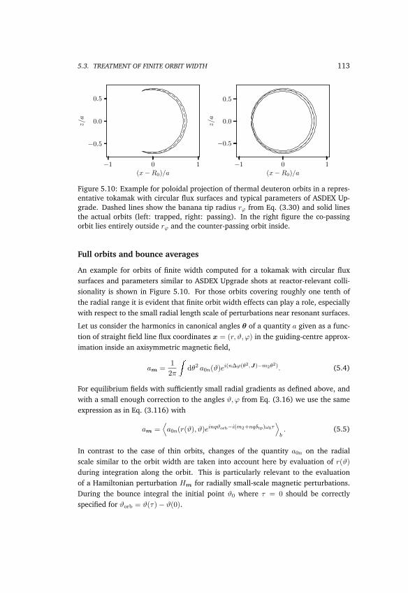
5.3. TREATMENT OF FINITE ORBIT WIDTH 113

−1 0 1

(x−R0)/a

−0.5

0.0

0.5

z/a

−1 0 1

(x−R0)/a

−0.5

0.0

0.5

z/a

Figure 5.10: Example for poloidal projection of thermal deuteron orbits in a repres-entative tokamak with circular flux surfaces and typical parameters of ASDEX Up-grade. Dashed lines show the banana tip radius rϕ from Eq. (3.30) and solid linesthe actual orbits (left: trapped, right: passing). In the right figure the co-passingorbit lies entirely outside rϕ and the counter-passing orbit inside.

Full orbits and bounce averages

An example for orbits of finite width computed for a tokamak with circular fluxsurfaces and parameters similar to ASDEX Upgrade shots at reactor-relevant colli-sionality is shown in Figure 5.10. For those orbits covering roughly one tenth ofthe radial range it is evident that finite orbit width effects can play a role, especiallywith respect to the small radial length scale of perturbations near resonant surfaces.

Let us consider the harmonics in canonical angles θ of a quantity a given as a func-tion of straight field line flux coordinates x = (r, ϑ, ϕ) in the guiding-centre approx-imation inside an axisymmetric magnetic field,

am =1

2π

dθ2 a0n(ϑ)ei(n∆ϕ(θ2,J)−m2θ2). (5.4)

For equilibrium fields with sufficiently small radial gradients as defined above, andwith a small enough correction to the angles ϑ, ϕ from Eq. (3.16) we use the sameexpression as in Eq. (3.116) with

am =⟨a0n(r(ϑ), ϑ)einqϑorb−i(m2+nqδtp)ωbτ

⟩b. (5.5)

In contrast to the case of thin orbits, changes of the quantity a0n on the radialscale similar to the orbit width are taken into account here by evaluation of r(ϑ)

during integration along the orbit. This is particularly relevant to the evaluationof a Hamiltonian perturbation Hm for radially small-scale magnetic perturbations.During the bounce integral the initial point ϑ0 where τ = 0 should be correctlyspecified for ϑorb = ϑ(τ)− ϑ(0).


0 1 2 3ϑorb

−0.050

−0.025

0.000

0.025

qϑorb−

∆ϕ

−5 0 5ϑorb

0.00

0.01

0.02

qϑorb−ωbτ−

∆ϕ

Figure 5.11: Examples of differences of the approximate and exact ∆ϕ to toroidalcanonical angle over ϑorb for parameters as in Figure 5.10 (left: trapped, right:passing). In the right plot the solid line shows the co-passing and the dashed linethe counter-passing orbit. Here the evaluation of q(ϑorb − ωbδtpτ) is performed forthe zero-order orbit at rϕ and the exact ∆ϕ is evaluated for the full orbit.

To illustrate the error that is introduced in the phase of the exponent in Eq. (5.5),Figure (5.11) shows the approximate deviation of the approximation ∆ϕ ≈ q(ϑorb−ωbδtpτ) from the exact quantity ∆ϕ = ϕ− θ3 = ϕ−Ω3τ . We can see that for typicaltoroidal mode-numbers n = 2 or n = 3 used for RMPs this error is sufficientlysmall to justify the use of Eq. (5.5) here. Problems with this approximation canpotentially arise very close to the trapped-passing boundary and for high toroidalmode-numbers n. In such cases the exact expression for ∆ϕ should be used insteadin Eq. (5.4).

Volume averaged conservation laws

Starting from a flux surface averaged conservation law, instead of setting rc(θ,J) ≈rϕ(pϕ) in expressions of the form of Eq. (4.24), we perform integrals along the fullorbit including radial drift away from the flux surface of r = rϕ. Physically thismeans that one orbit contributes to sources on all flux surfaces that it passes duringits bounce or transit period. To resolve the term δ(rc(θ,J) − r) inside the fluxsurface average, we introduce another average over a finite radial region betweenflux surfaces at radius ra and rb,

〈A〉ab ≡1

∆rab

rb

ra

dr 〈A〉 (5.6)

=1

∆rab

rb

ra

dr1

S(r)

d3θ

d3J δ(rc(θ,J)− r)a(rc(θ,J)) f(t,θ,J). (5.7)

Here the integral describing volumetric contributions between ra and rb is normal-ised by the radial distance ∆rab = rb − ra. This makes expressions directly com-parable to their radially local counterparts in the limiting case of zero orbit width

5.3. TREATMENT OF FINITE ORBIT WIDTH 115

together with ∆rab → 0, where all contributions come from a single flux surface withr = ra = rb = rϕ. In particular, for the toroidal torque density given in Eq. (4.69),we have

〈Tϕ〉ab = − 1

∆rab

∑m

n

rb

ra

dr1

S(r)

d3θ

d3J δ(rc(θ,J)− r)Qm(J). (5.8)

An exact computation with flux surface area S from Eq. (4.17) is possible, but a fur-ther simplification can be made if ∆rab is smaller than the characteristic length scaleof the equilibrium field. Since we will choose it to be of similar or smaller order thanthe orbit width ∆rmax

c . 2 ·max |rc − rϕ| at thermal velocity, this condition is wellfulfiled within the approximation defined earlier and we set S(r) ≈ S((ra+rb)/2) ≡Sab. A next order approximation would be a correction due to the geometric scalingS ∝ r2 from Eq. 4.17, which is not considered here. Consequently, the constantterm 1/Sab can be extracted as a common factor in Eq. (5.7). Keeping the angulardependency only for the canonical bounce phase θ2 relevant for guiding-centre mo-tion in the unperturbed axisymmetric field and changing one integration variablefrom J3 = pϕ to rϕ with first derivative p′ϕ(rϕ) from Eq. (3.31) yields

〈Tϕ〉ab =− (2π)2

Sab∆rab

∑m

n

dJ⊥

dJϑ

dθ2

rb

ra

dr

drϕ

∣∣p′ϕ(rϕ)∣∣ δ(rc(θ2,J)− r)Qm(J). (5.9)

The integral over r is resolved via the general relation

dθ2

rb

ra

dr

drϕδ(rc(θ

2, rϕ)− r)g(rϕ) = (θ2b − θ2

a)

drϕ

g(rϕ) if rc ∈ (ra, rb)

0 otherwise

(5.10)

Here we have formally omitted the notation of dependencies on J⊥ and Jϑ. Regard-ing the canonical bounce phase θ2, no explicit dependency remains from Eq. (5.9),making integration trivial. We notice that the term

(θ2b − θ2

a) = 2π∆τabτb

(5.11)

measures the fraction of the bounce time τb of the full orbit spent between radius raand rb. The evaluation of integrals over rϕ is possible to second-order accuracy viathe midpoint rule

drϕg(rϕ) ≈

∑i

∆riϕ gi, (5.12)


with gi = g((riϕ + ri−1ϕ )/2) evaluated at the midpoint of each interval (ri−1

ϕ , riϕ).Though not strictly necessary, we choose an equidistant grid with Nr steps, whichwe use also to define a set of intervals (ra, rb) for the evaluation of locally volume-averaged torque densities.1 This simplifies expressions such as Eq. (5.9) by thecancellation of ∆rab = ∆riϕ = ∆r. In addition, for the special case ∆r > ∆rmax

c

it leads to orbits that are respectively contained in single intervals (ra, rb) with rϕ

centred in-between and ∆τab = τb, which represents a natural connection to thelimiting case of thin orbits. To sum up, the volume-averaged quasilinear toroidaltorque density between two sufficiently close flux surfaces a and b of Eq. (5.9) canbe represented by

〈Tϕ〉ab =− (2π)3

Sab

Nr∑i=1

∆τabτb

∣∣p′iϕ∣∣∑m

n

dJ⊥

dJϑQ

im. (5.13)

The result is the analogue to Eq. (4.70) for orbit widths that are comparable to theradial perturbation scale. Because of the assumption of sufficiently large-scale equi-librium field it is still possible to formally define radially local transport coefficientsas defined in section 4.8 for computations. However, due to the radially non-localnature of the toroidal momentum source in Eq. (5.13), the direct presentation of〈Tϕ〉ab appears more suited for a straightforward physical interpretation.

5.4 Summary and Outlook

Within this text, a unified description of low-collisional quasilinear and non-linearresonant transport regimes leading to neoclassical viscous torque in tokamak plas-mas with non-axisymmetric magnetic perturbations has been developed. The methodtakes into account the full device geometry and follows from Hamiltonian perturb-ation theory in action-angle coordinates in combination with kinetic theory. Thisallows for a physically justifiable transition between quasilinear and non-linear re-gimes.

The general form of the method has been described independently from the specificproblem. Here, the transition of a dimensionless perturbation of the distributionfunction between quasilinear and non-linear limit has been illustrated. From thisgeneral result, a non-linear attenuation factor for the actual problem of toroidaltorque has been derived. This factor can be tabulated as a function of a parameterdepending on collisionality and perturbation amplitude from a numerical solutionof the general form of the dimensionless perturbed kinetic equation.

To allow the application of the method, exact expressions for action-angle variablesin a tokamak have been constructed based on the guiding-centre Lagrangian in

1Actual computations are performed on an equidistant grid in ψtor rather than reff from Eq. (4.16).

5.4. SUMMARY AND OUTLOOK 117

straight field line magnetic flux coordinates. For efficient numerical computationof canonical (bounce and drift) frequencies, a first-order expansion in orbit widthis employed later. In this formalism, a magnetic shear term, that is absent in thestandard local neoclassical ansatz, appears naturally.

The obtained expressions for canonical frequencies and transport coefficients havebeen validated against existing works analytically and numerically and have beenshown to match in the common range of applicability. Based on the Hamiltonian ap-proach, the code NEO-RT has been developed and applied on a model tokamak andASDEX Upgrade with resonant magnetic perturbations. The features included in theHamiltonian approach, namely full geometry, magnetic drift, magnetic shear, andnon-linear attenuation have been demonstrated to be relevant in those cases. Theclose match with results from the quasilinear version of the code NEO-2 possessinga full (energy- and momentum-conserving) collision operator verify the theoreticalresult of the negligible role of momentum conservation in the collision model forresonant transport regimes at sub-sonic toroidal rotation.

A major limitation for the applicability of the method to compute non-linear atten-uation are well-separated resonances in phase-space. Close to the zero-crossing ofthe radial electric field with main contributions from the superbanana resonance,this is the case. Otherwise, for drift-orbit resonances, this can be safely assumed inanalogy to the pendulum Hamiltonian as long as the dominant resonances are farfrom the trapped-passing boundary. If this is not the case, further analysis of theChirikov criterion on the width and distance of resonances is necessary.

Besides the possible consideration of the effect of finite orbit width on canonicalfrequencies and angles, further analysis of the radial width of super-orbits is re-quired when approaching the non-linear limit. The used concepts permit also anextension to consider effects from a non-negligible Larmor radius compared to char-acteristic length scales of the perturbation. In the latter case, the largeness of thegyrofrequency would allow for simplifications while spatial finite-Larmor-radius ef-fects could be fully taken into account. Also, the extension to faster toroidal rotationis possible, where the radial electric field has a non-negligible influence on the par-allel motion of the full orbit. Those are possible points to be treated in the future tobetter judge the range of applicability of the Hamiltonian approach and to balanceaccuracy against computation time.

Appendix A

Construction of magnetic fluxcoordinates

Magnetic flux coordinates D’haeseleer et al. (1991) where field lines become straightin coordinate space are required for the formulation of the described methodologyformulated on curved magnetic geometries. In this appendix the general form offlux coordinates and their most important properties will be outlined.

A.1 Clebsch Form

The zero-divergence condition for magnetic fields is implicitly given by writing thefield in Clebsch form,

B =∇r ×∇ν. (A.1)

Here, r is an arbitrary radial coordinate withB = const. and ν(r, ϕ, ϑ) can be writtenas a function of r and two angle coordinates ϕ and ϑ.

The divergence of the magnetic field is then given by

∇ ·B = ∇ · (∇r ×∇ν) = (∇ · (∇r)︸︷︷︸=0

)×∇ν +∇r × (∇ · (∇ν)︸︷︷︸=0

) = 0.

Contravariant coordinates are given by first derivatives of the function ν,

B =1√gεijk (∂ir∂jν) ek (A.2)

Br = 0 (A.3)

Bϕ =1√g∂ϑν (A.4)

Bϑ = − 1√g∂ϕν. (A.5)

120 APPENDIX A. CONSTRUCTION OF MAGNETIC FLUX COORDINATES

The periodicity condition

B(r0, ϕ, ϑ) = B(r0, ϕ+ 2π, ϑ) = B(r0, ϕ, ϑ+ 2π) (A.6)

can be fulfiled if ν is a sum of linear terms in the angle variables and a periodicfunction ν,

ν(r, ϕ, ϑ) = a(r)ϕ+ b(r)ϑ+ ν(r, ϕ, ϑ) (A.7)

For a linear function in ϕ and ϑ,

ν(r, ϕ, ϑ) = c(r) + a(r)ϕ+ b(r)ϑ,

the gradient is given by

∇ν = (c′(r) + a′(r)ϕ+ b′(r)ϑ)∇r + a(r)∇ϕ+ b(r)∇ϑ.

The magnetic field (A.1) is still periodic, since

∇r ×∇ν = (c′(r) + a′(r)ϕ+ b′(r)ϑ)(∇r ×∇r︸︷︷︸=0

) + a(r)∇r ×∇ϕ+ b(r)∇r ×∇ϑ

= a(r)∇r ×∇ϕ+ b(r)∇r ×∇ϑ.

Adding higher terms to ν, e.g. ϕ2 results in a non-periodic field in the angle vari-ables,

∇r ×∇(d(r)ϕ2) = (d′(r)ϕ2)(∇r ×∇r) + d(r)ϕ

2∇ϕ.

A.2 Magnetic flux

Introducing toroidal and poloidal fluxes by integration over toroidal and poloidalsurfaces,

ψtor(r) =1

2π

Stor

B · dS =1

(2π)2

VB · ∇ϕ dV, (A.8)

ψpol(r) =1

2π

Spol

B · dS =1

(2π)2

VB · ∇ϑ dV. (A.9)

The equivalence of these volume and surface integrals may be illustrated for a tor-oidal surface: We cut the torus at a given toroidal surface with ϕ = 0 and evaluatethe integral

torus

ϕB · dS =

V∇(ϕB) dV =

VB · ∇ϕ dV (A.10)

A.2. MAGNETIC FLUX 121

along a closed toroidal surface, ending at the cut with ϕ = 2π and use Stokes’theorem and ∇ ·B = 0. The left side can be split into

−ϕ=0

ϕB · dS +

Storus

ϕB · dS +

ϕ=2π

ϕB · dS.

The first term vanishes because of ϕ = 0, the second term because of the field linesof B going along the toroidal surface. The remaining term

ϕ=2π

ϕB · dS = 2π

Stor

B · dS

for the toroidal surface Stor at ϕ = 2π can thus be expressed by the volume integral(A.10).

The fluxes (A.8) and (A.9) correspond to the functions a(r) and b(r): The firstderivative of the toroidal flux with respect to r is

ψ′tor(r) =dψtor

dr=

1

(2π)2

d

dr

r

0dr′

2π

0dϕ

2π

0dϑ√gB · ∇ϕ

=1

(2π)2

2π

0dϕ

2π

0dϑ√gB · ∇ϕ

=1

(2π)2

2π

0dϕ

2π

0dϑ√gBϕ

=1

(2π)2

2π

0dϕ

2π

0dϑ∂ϑν

=1

(2π)2

2π

0dϕ

2π

0dϑ (b(r) + ∂ϑν(r, ϕ, ϑ)) .

Since the integral over the second term vanishes, we can identify

ψ′tor(r) = b(r).

Similarly, it can be shown that

ψ′pol = −a(r)

and finally, 120 can be written as

ν(r, ϕ, ϑ) =ψ′tor(r)ϑ− ψ′pol(r)ϕ+ ν(r, ϕ, ϑ). (A.11)

122 APPENDIX A. CONSTRUCTION OF MAGNETIC FLUX COORDINATES

A.3 Transformation to flux coordinates

If ν vanishes, the coordinates (r, ϕ, ϑ) are called flux coordinates and the magneticfield can be written in the simple form

B = ∇ϕ×∇ψpol(r) +∇ψtor(r)×∇ϑ= −ψ′pol(r)∇r ×∇ϕ+ ψ′tor(r)∇r ×∇ϑ= ∇r ×∇(ψ′tor(r)ϑ− ψ′pol(r)ϕ).

=ψ′pol(r)√

gEϑ +

ψ′tor(r)√gEϕ. (A.12)

In flux coordinates, magnetic field lines are straight lines due to

Bϕ = qBϑ, (A.13)

where q is known as the the safety factor, given by the ratio

q =ψ′tor(r)

ψ′pol(r). (A.14)

A corresponding vector potential is given by

A(r) =ψtor(r)∇ϑ− ψpol(r)∇ϕ. (A.15)

Although it would be straightforward to use a vector potential

A = −ν(r)∇r,

this form has the problem of non-uniqueness with respect to the angular coordinates.

Transformation from non-flux coordinates to flux coordinates is possible by a changeof one of the two angle coordinates that cancel out the periodic part in (A.11), either

ϑ = ϑ0 +ν(ρ, ϕ, ϑ)

ψ′tor(r)(A.16)

or

ϕ = ϕ0 −ν(ρ, ϕ, ϑ)

ψ′pol(r). (A.17)

Appendix B

Analytical comparison to existingresults

Results for quasilinear diffusion in the superbanana plateau regime have been pub-lished by Shaing et al. (2009b) for the large-aspect-ratio approximation with circularflux surfaces and in Shaing (2015) for arbitrary tokamak geometries. The resonantplateau regime by bounce-transit and drift resonances has been analysed in Sha-ing et al. (2009a) for the large-aspect-ratio limit with circular flux surfaces. In thoseworks, Hamada coordinates are used with the normalized enclosed volume r = V =

V/4π2 as the radial variable, metric determinant√gH = 1 and contravariant com-

ponents of the magnetic field constant on a flux surface with Bϑ = ψ′pol, Bϕ = ψ′tor.

This leads to a specific form of a number of formulas, including the bounce average3.90 omitting the sign σ with

τb =

dϑ

v‖hϑ=

dϑ

B

v‖ψ′pol

, (B.1)

〈a〉b =

dϑ

a

v‖hϑ=

dϑ

B

v‖ψ′pol

a . (B.2)

B.1 Toroidal drift frequencies

First, we compare the present toroidal drift frequencies to the ones given by Shaing(2015). Formula (10) of this reference contains the bounce averaged toroidal driftfrequency as defined in (3.102), which, in our notation, is written as

ΩtE =cΦ′

ψ′pol

, (B.3)

〈ΩtB〉b = − 1

ψ′pol

⟨J⊥ωc +mv2

‖mωc

∂B

∂r−v2‖ωc

1

B

∂(B2)

∂r+v2‖ωc

ψ′′pol

ψ′pol

B

⟩b

. (B.4)

124 APPENDIX B. ANALYTICAL COMPARISON TO EXISTING RESULTS

The pressure P has been set to zero here, since we consider orbits directly in theactual equilibrium where finite β effects are implicitly included. Shaing definesthe magnetic moment µ without mass, which leads to the additional factor whenchanging to the notation using the perpendicular invariant J1 = J⊥. In addition,the signs are swapped due to the definition of the toroidal angle ϕ0 in the oppositedirection. Using B2 = Bϑ (Bϑ + qBϕ) we can write

ψ′′pol =dBϑ

dr=

d

dr

(B2

Bϑ + qBϕ

)= − B2

(Bϑ + qBϕ)2

∂

∂r(Bϑ + qBϕ) +

1

Bϑ + qBϕ

∂(B2)

∂r

= − 1

Bϑ + qBϕ

(Bϑ ∂

∂r(Bϑ + qBϕ) +

∂(B2)

∂r

). (B.5)

Also,

ψ′′pol

ψ′pol

B =B

Bϑ (Bϑ + qBϕ)

(−Bϑ ∂

∂r(Bϑ + qBϕ) +

∂(B2)

∂r

)=

1

B

(−Bϑ ∂

∂r(Bϑ + qBϕ) +

∂(B2)

∂r

). (B.6)

The last term cancels out with the middle term in Eq. (B.4), so we obtain

〈ΩtB〉b =1

ψ′pol

⟨−J⊥ωc +mv2

‖mωc

∂B

∂r+v2‖ωchϑ(∂Bϑ∂r− q∂Bϕ

∂r− dq

drBϕ

)⟩b

,(B.7)

which is identical to the bounce-averaged magnetic drift frequency in Eq. (3.105).In particular, the radial derivative of the safety factor (magnetic shear) is present asit appears in the second derivative in the poloidal flux ψ′′pol in Eq. (B.4).

B.2 Bounce integrals in the large-aspect-ratio limit

For a circular concentric flux surface, the unperturbed magnetic field modulus iswritten as

B = Ba(1− ε cosϑ) , (B.8)

with magnetic field modulusBa on axis and aspect ratio ε relating flux surface minorradius to the device major radius. With κ = k2 from Shaing et al. (2009a), bounceintegrals are given by

dϑ

v‖hϑa(ϑ) =

√mα

4µBaε

1

ψ′pol

dϑ

Ba(1− ε cosϑ)√κ− sin2 ϑ

2

a(ϑ) . (B.9)

B.2. BOUNCE INTEGRALS IN THE LARGE-ASPECT-RATIO LIMIT 125

In the large aspect ratio limit the ε term is neglected and the bounce time in Eq.(B.1) for trapped particles becomes

τb =

√mα

4µBaε

Baψ′pol

dϑ√

κ− sin2 ϑ2

=

√mα

µBaε

Baψ′pol

4K(κ) . (B.10)

Here the integral is performed over the full orbit, so twice between the turningpoints defined by

sin2 ϑ±

2= κ (B.11)

⇒ ϑ± = ±2 arcsin√κ . (B.12)

(0 < κ < 1 for trapped particles). In the notation of Shaing, a bounce integral isperformed just once between ϑ+ and ϑ−. Finally we obtain an expression for bounceaveraging in the large aspect ratio as

〈a〉b =1

4K(κ)

ϑ+

ϑ−

dϑa(ϑ)√κ− sin2 ϑ

2

. (B.13)

This means that we have to replace K(κ) in the formulas of Shaing et al. (2009a)by

K(κ) =τb4

√µBaε

mα

ψ′pol

Ba(B.14)

to translate to the notation of the present work.

The bounce integration for passing particles is formally identical to trapped particlesbut performed over the full range in ϑ where v‖ doesn’t change sign (κ > 1) .

Using the same approximation as in Eq. (B.10), the bounce (transit) time for passingparticles is

τb =4K(κ−1)

κ

√mα

4µBaε

Baψ′pol√

mα

µBaε

Baψ′pol

2K(κ−1)√κ

. (B.15)

in the large-aspect-ratio limit. Due to the mathematical equivalence of the guiding-centre motion in the large-aspect-ratio limit with circular, concentric flux surfaces tothe particle in a cosine potential (pendulum), those bounce times represent an exactanalogy to the ones in section 1.3, differing only by a normalisation factor.


For integrations we use the transformations

x = u2, (B.16)

dx = 2udu, (B.17)

v2‖ = 4

µBaε

mα

(κ− sin2 ϑ

2

)= (1− ηB0)u2v2

T , (B.18)

κ =H0 − eαΦ− µBa(1− ε)

2µBaε(B.19)

with

µ =mu2

2v2t η =

mx

2v2t η. (B.20)

We get

κ =1− ηBa(1− ε)

2ηBaε(B.21)

=1/η −Ba(1− ε)

2Baε. (B.22)

The derivative is

dκ

dη= − 1

2η2Baε. (B.23)

From this section it is clear that we can use expressions (8) and (33) of Shaing et al.(2009a) as the equivalent to the poloidal canonical angle of Eq. (3.76) here. Usingthe variable transformation for integrals in velocity space allows us to translate fromviscous coefficients µij in the reference to our expressions for transport coefficientsDij of Eq. (4.84), what will be done in the following section.

B.3 Eulerian approach to drift-orbit resonances

Shaing et al. (2009a) constructs the Eulerian approach for drift-orbit resonancesneglecting magnetic drifts. We write the drift-kinetic equation with mass flow as inShaing and Spong (1990); Shaing (1990) referring to Hazeltine and Ware (1978)as

(v‖ + vd + V ) · ∇f + w∂f

∂w= C(f), (B.24)

where the velocity space coordinates are w = v2/2 and µ = v2⊥/(2B). The parallel

velocity is given by v‖ = v‖b =√

(1/2− µB)wb. (In the review paper Shaing et al.

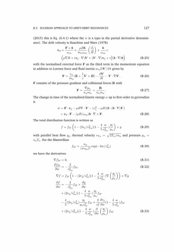
B.3. EULERIAN APPROACH TO DRIFT-ORBIT RESONANCES 127

(2015) this is Eq. (6.4.1) where the w is a typo in the partial derivative denomin-ator). The drift velocity is Hazeltine and Ware (1978)

vd =F× bωcα

+µBb

mαωcα

(J‖B

)+

b

ωcα×(

µ∇B + (v‖ · ∇)V + (V · ∇)v‖ + v2‖(b · ∇)b

)(B.25)

with the normalised external force F as the third term in the momentum equationin addition to Lorentz force and fluid inertia mαDV /Dt given by

F =eαmα

(E +1

cV ×B)− ∂V

∂t− V · ∇V . (B.26)

F consists of the pressure gradient and collisional forces R with

F =∇pαnαmα

+R

nαmα. (B.27)

The change in time of the normalised kinetic energy w up to first order in gyroradiusis

w = F · v‖ − µB∇ · V − (v2‖ − µB)(b · (b · ∇)V )

+ vd · F− (µB/ωcα)b · ∇ × F. (B.28)

The total distribution function is written as

f = fM

(1− (2v‖/v

2Tα)(1− 4

5

w

v2Tα

)q‖pα

)+ g (B.29)

with parallel heat flow q‖, thermal velocity vTα =√

2Tα/mα and pressure pα =

nαTα. For the Maxwellian

fM =nα

(πvtα)3exp(−2w/v2

tα) (B.30)

we have the derivatives

∇fM = 0, (B.31)∂fM∂w

= − 2

v2Tα

fM , (B.32)

∇f = fM

(1− (2v‖/v

2tα)(1− 4

5

w

v2Tα

)∇(q‖pα

))+∇g

∂f

∂w= − 2

v2Tα

fM +∂g

∂w

+ (2v‖/v2tα)(1− 4

5

w

v2Tα

)q‖pαfM

− 4

5(2v‖/v

2tα)

q‖pαv2

tα

fM +2

v2t

∂v‖∂w

(1− 4

5

w

v2tα

)fM

+ (2v‖/v2Tα)(1− 4

5

w

v2Tα

)∂

∂w

(q‖pα

)fM . (B.33)


Of course, for the Maxwellian C(fM ) = 0. For now, we ignore the terms related tothe heat flux and write

(v‖ + vd + V ) · ∇g + w∂g

∂w− C(g) = − 2

v2tα

fM ·

(F · v‖ − µB∇ · V − (v2‖ − µB)(b · (b · ∇)V )

+vd · F− (µB/ωcα)b · ∇ × F)− C(fM ). (B.34)

C(fM ) is not zero for finite V . The first term arising from in w ∂fM∂w is

−2v‖v2Tα

b ·Rnαmα

fM = −v‖b ·Rpα

fM

and should cancel C(fM ). The remaining assumptions are ∇pα · b = 0, ∇pα ×∇Tα = 0, ∇ · V = 0, ∇q = 0 and neglecting viscous forces. The remaining term is(v2‖ − µB)(b · (b · ∇)V ). We write

v2‖ − µB = v2

‖ −v2 − v2

‖2

=3

2v2‖ −

1

2v2

= −v2

(1

2− 3

2

v2‖v2

). (B.35)

Finally

(v‖ + vd + V ) · ∇g + w∂g

∂w− C(g) =

2v2

v2Tα

(1

2− 3

2

v2‖v2

)(b · (b · ∇)V )fM . (B.36)

We note that for ∇ · V = 0 and ∇ ·B = 0

b · (b · ∇)V =1

BV · ∇B. (B.37)

Including heat fluxes, the final expression is

(v‖ + vd + V ) · ∇g + w∂g

∂w− C(g) =

2v2

v2Tα

(1

2− 3

2

v2‖v2

)(V · ∇BB

− (2v‖/v2Tα)(1− 4

5

w

v2Tα

)q · ∇BBpα

)fM . (B.38)

In Shaing et al. (2009a), Eq. (3), the flow velocity is split into parallel and perpen-dicular part from E×B drift and vd · ∇g is neglected, with

(v‖ + vd + V ) · ∇g ≈ ((v‖ + V‖)b+ V E) · ∇g. (B.39)

B.3. EULERIAN APPROACH TO DRIFT-ORBIT RESONANCES 129

Derivations by Shaing are done in Hamada coordinates. We translate the normalisedvolume coordinate V = V/4π2 (used by Shaing to get

√gH = 1 and called V there)

to the normalised flux s as the radial coordinate with

ψ′(V ) = ψ′tor(s)ds

dV= q(s)ψ′pol(s)

ds

dV, (B.40)

χ′(V ) = ψ′pol(s)ds

dV. (B.41)

Primes on ψ and χ are defined w.r.t. V , otherwise to s. In Kasilov et al. (2014)velocity components are listed as

V ϑ =ckBϕ

eα√g 〈B2〉

∂Tα∂s

=ckBϕTαeα√g 〈B2〉A2, (B.42)

V ϕ =c√gBϑ

(−∂Φ

∂s− 1

eαnα

∂pα∂s

)+ qV ϑ

= − c√gBϑ

Tαeα

(eαTα

∂Φ

∂s+

1

nα

∂nα∂s

+1

Tα

∂Tα∂s

)+ qV ϑ

= − c

ψ′pol

Tαeα

(A1 +

5

2A2

)/ 〈|∇s|〉+ q

ckBϕTαeα√g 〈B2〉A2/ 〈|∇s|〉 . (B.43)

Here, thermodynamic forces are defined as

A1/ 〈|∇s|〉 =1

nα

∂nα∂s

+eαTα

∂Φ

∂s− 3

2

1

Tα

∂Tα∂s

=1

pα

∂pα∂s

+eαTα

∂Φ

∂s− 5

2

1

Tα

∂Tα∂s

, (B.44)

A2/ 〈|∇s|〉 =1

Tα

∂Tα∂s

. (B.45)

Notice that

1

pα

∂pα∂s

=1

nαTα

∂

∂s(nαTα) =

1

nα

∂nα∂s

+1

Tα

∂Tα∂s

. (B.46)

The validity of (B.42) and (B.43) arises from the divergence-free plasma flow velo-city V which is given by Shaing et al. (2010)

V = V‖h+ V ⊥, (B.47)

V ⊥ = cb×∇Φ

B2+ c

b×∇pαNeαB2

. (B.48)

Its components are related to the gradients and thus to thermodynamic forces with

− eαcTα

(χ′(V )V ϕ − ψ′(V )V ϑ

)=

1

pα

∂pα

∂V+eαTα

∂Φ

∂V, (B.49)


so in our notation

eαcTα

(ψ′pol(s)V

ϕ − ψ′tor(s)Vϑ)

=1

pα

∂pα∂s

+eαTα

∂Φ

∂s

=1

nαTα

∂

∂s(nTα) +

eαTα

∂Φ

∂s

=1

nα

∂nα∂s

+1

Tα

∂Tα∂s

+eαTα

∂Φ

∂s. (B.50)

we obtain

eαcTα

ψ′pol

(qV ϑ − V ϕ

)〈|∇s|〉 = A1 +

5

2A2, (B.51)

which is in accordance with the above results. Shaing et al. (2009a) define coeffi-cients µ for the neoclassical toroidal plasma viscosity by

〈bt · ∇ · π〉 = µp1V · ∇ϑ+ µt1V · ∇ϕ+2

5µp2

q · ∇ϑpα

+2

5µt2q · ∇ϕpα

. (B.52)

The task is, to relate µ coefficients to D11 and D12. We use the flux-force relationShaing et al. (2009b)

Γ =c

eαχ′ψ′〈bt · ∇ · π〉 (B.53)

and neglect the smaller last two terms containing heat fluxes in (B.52) to write

c

eαqψ′2pol

(µp1V

ϑ + µt1Vϕ)(dV

ds

)2

= −nα(D11A1 +D12A2). (B.54)

=c

eαqχ′2

(µp1V

ϑ + µt1Vϕ)

(B.55)

We insert expressions (B.42) and (B.43) to obtain

D11A1 +D12A2 =

(dV

ds

)21

〈|∇s|〉

[−µp1

1

qψ′2pol

c2kBϕTαnαe2

α√g 〈B2〉A2

+µt1c2

qψ′3pol

Tαnαe2

α

(A1 +

5

2A2

)− µt1

1

ψ′2pol

c2kBϕTαnαe2

α√g 〈B2〉A2

].

(B.56)

B.4. TRANSPORT COEFFICIENTS FOR BOUNCE-DRIFT RESONANCES 131

So for the coefficients we have

D11 =

(dV

ds

)21

〈|∇s|〉c2Tα

nαe2αqψ

′3pol

µt1 ≡ Aµt1, (B.57)

D12 =

(dV

ds

)21

〈|∇s|〉

[− 1

qψ′2pol

c2kBϕTαnαe2

α√g 〈B2〉µp1

+

(5

2

c2Tαnαe2

αqψ′3pol

− 1

ψ′2pol

c2kBϕTαnαe2

α√g 〈B2〉

)µt1

](B.58)

≡ Cµp1 +

(5

2A− qC

)µt1 (B.59)

= Cµp1 +

(5

2− qC

A

)D11 (B.60)

with

A =

(dV

ds

)21

〈|∇s|〉c2Tα

nαe2αqψ

′3pol

, (B.61)

C = −(dV

ds

)21

〈|∇s|〉1

qψ′2pol

c2kBϕTαnαe2

α√g 〈B2〉 . (B.62)

In the following section, we will explicitly compare Eq. (4.84) to Eq. (27) of Shainget al. (2009b).

B.4 Transport coefficients for bounce-drift resonances

Using the large-aspect ratio expressions for bounce resonances, we can transformtransport coefficients from the quasilinear Hamiltonian formalism to

D1k =π3/2n2c2vT

e2α 〈|∇s|〉2 ψ′pol(s)

ds

dV

∞0

du (B.63)

u3e−u2∑m2

∑res

(τb|Hm|2

∣∣∣∣m2∂ωb∂η

+ n∂Ω3

∂η

∣∣∣∣−1)η=ηres

wk

=1

4√π

n2c2vTBa

e2α 〈|∇s|〉2 ψ′2pol

∞0

du

√mα

µBaεu3e−u

2∑m2

∑res

(4K(κ)|Hm|2

∣∣∣∣m2∂ωb∂η

+ n∂Ω3

∂η

∣∣∣∣−1)η=ηres

wk

=1

2√π

n2c2vTBa

e2α 〈|∇s|〉2 χ′2

(ds

dV

)2 ∞0

dx√mα

µBaεxe−x

∑m2

∑res

(K(κ)|Hm|2

∣∣∣∣m2∂ωb∂η

+ n∂Ω3

∂η

∣∣∣∣−1)η=ηres

wk.


The derivative in the resonance condition is

∂

∂η(nΩtE +m2ωb) =

∂κ

∂η

∂

∂κ

(−n c

ψ′pol

∂Φ

∂s+m2

π

2K(κ)

√µBaε

mα

ψ′pol

Ba

ds

dV

)(B.64)

=− 1

2η2Baε

∂

∂κ

(−n c

χ′∂Φ

∂V+m2

π

2K(κ)

√µBaε

mα

χ′

Ba

)

=m2

2η2Baε

∂

∂κ

[√µBaε

mα

χ′

Ba

(n

m2

c

χ′

√mα

µBaε

Baχ′

∂Φ

∂V− π

2K(κ)

)]

≈m2vtχ′

2ε

√xε

2

∂

∂κ

[n

m2

√2Ba√xεχ′

c

χ′∂Φ

∂V− π

2K(κ)

]=m2vtχ

′

2ε

√xε

2

∂Gnm2

∂κ

where we assumed for trapped particles in the large aspect ratio limit that

µBa ≈mαx

2v2t (B.65)

⇒ ηBa ≈ 1 (B.66)

⇒√µBaε

mα≈√xε

2vt (B.67)

⇒ τb ≈ 4K(κ)

√2

xε

Bavtχ′

. (B.68)

We can write D1k as

D1k =1

2√π

n2c2Ba

e2α 〈|∇s|〉2 χ′2

(ds

dV

)2 ∞0

dx√2

xεxe−x

∑m2

∑res

(K(κ)|Hm|2

∣∣∣∣m2vtχ′

2ε

√xε

2

∂Gnm2

∂κ

∣∣∣∣−1)η=ηres

wk

=√π

n2c2Ba

e2α 〈|∇s|〉2 χ′2vt

(ds

dV

)2 ∞0

dx

e−x∑m2

∑res

(K(κ)

π/2|Hm|2

∣∣∣∣m2χ′∂Gnm2

∂κ

∣∣∣∣−1)η=ηres

wk (B.69)

The perturbation defined by Shaing is

1

B

∂B

∂θ3=∑n,m2

inBnB

=∑n,m2

bnm2ei(m2θ2+nθ3), (B.70)

B

B0=

B

Ba + ε cosϑ=

B

Ba− B cosϑ

2Ba2ε+O(ε2)

=B

Ba+O(εB/Ba) +O(ε2) ≈ B

Ba. (B.71)

B.4. TRANSPORT COEFFICIENTS FOR BOUNCE-DRIFT RESONANCES 133

We compare this to the Hamiltonian perturbation

H =

(mαv

2‖(ϑ) +

eαmαc

J⊥B0(ϑ)

)B

B0(B.72)

≈ mαxv2t

2

B

Ba(B.73)

⇒ Hm2n =mαxv

2t

2

bnm2

in(B.74)

Note, that one has to be careful with the sign convention because Shaing defines

B = −εmn exp(mϑ− nζ), (B.75)

ζ0 = qϑ− ζ, (B.76)

ωE = +cΦ′

χ′. (B.77)

If one uses ζ = −ϕ we get the usual expansion and canonical angle (to the lowestorder in Larmor radius) with

B = −εmn exp(mϑ+ nϕ), (B.78)

θ3 ≡ ζ0 = qϑ+ ϕ. (B.79)

The minus sign for the perturbation does not cause any troubles, because we includeit in B. Inserting this in the transport coefficient expression yields

D1k =

√π

4

m2α|n|c2Bav

3t

e2α 〈|∇s|〉2 χ′2

(ds

dV

)2 ∞0

dx

x2e−x∑m2

∑res

(K(κ)

π/2|bnm2 |2

∣∣∣∣m2χ′∂Gnm2

∂κ

∣∣∣∣−1)η=ηres

wk. (B.80)

For µt1 we obtain

µt1 = nαmαvt

√π

2Ba

ψ′

|χ′|1

〈|∇s|〉∂s

∂V

∞0

dx

x2e−x∑m2

|n||m2|

∑res

(K(κ)

π/2|bnm2 |2

∣∣∣∣∂Gnm2

∂κ

∣∣∣∣−1)η=ηres

. (B.81)

There is a difference in the definition of fluxes by Shaing as he uses a total fluxΓShaing with normalisation to the Volume V = 4π rather than our flux density Γus asin Eq. (4.83). The relation is

ΓShaing = SΓus (B.82)

Shaing uses

ΓShaing = Γ · ∇V (B.83)


whereas we take

Γus = Γ · ∇r (B.84)

with the effective radius r defined by

∇V = S∇r (B.85)

or

∇V = S∇r (B.86)

If we take s as the radial variable, we get

ΓShaing =∂V

∂s

∂r

∂sΓus =

∂V

∂s

1

〈|∇s|〉Γus.

Thus, the results are matching. In the large aspect ratio limit, we have

V ≈ 4π2R0r, (B.87)

S =dV

dr≈ R0 =

r

ε. (B.88)

For the effective radius r we use the translation

〈|∇s|〉 =ds

dr=

ds

dV

dV

dr≈ R0

ds

dV. (B.89)

To sum up, we have proven the consistency of viscous coefficient µt1 for trappedparticles in Eq. (27) Shaing et al. (2009b) with our expression for transport coeffi-cients of Eq. (4.84).

B.5 Expressions for the transit-drift resonance

In the same matter as in the previous sections, terms for transport coefficients canbe compared for the transit-drift resonance of passing particles. As we will see, thearticle of Shaing et al. (2009a) contains an inconsistency with regard to Fourierintegrals, which will become clear below.

The bounce integration for passing orbits is formally similar to trapped orbits butperformed over the full range in ϑ where v‖ doesn’t change sign (κ > 1). We startfrom the resonance condition

∂

∂η(nΩtE + (m2 + nq)ωb) =

B.5. EXPRESSIONS FOR THE TRANSIT-DRIFT RESONANCE 135

1

2η2κ2Baε

∂

∂(1/κ)

(−n c

χ′∂Φ

∂V+ 2 (m2 + nq)

√µBaε

mα

χ′

Ba

π√κ

2K(1/√κ)

)

= − 1

2η2κ2Baε

∂

∂(1/κ)

(nc

χ′∂Φ

∂V− 2 (m2 + nq)

√εxv2

t /2

2εκ+ (ε− 1)

χ′

Ba

π√κ

2K(1/κ)

)

=m2√xvt

2η2κ2Baε

χ′

Ba

∂

∂(1/κ)

(n

m2

c√xvtχ′

Baχ′

∂Φ

∂V−(

1 +n

m2q

)√2εκ

2εκ+ (ε− 1)

π

2K(1/κ)

)(B.90)

Our term with nq is not present in Shaing’s paper in (45). The reason for this lies inhis Fourier expansion of a non-periodic function.

For circulating particles in (35) and (39) one should obtain

σ(l − nq)ωt + nωE (B.91)

instead of

σlωt + nωE (B.92)

in the perturbed solution gnl. The reason for that is the following:

To have the correct periodicity for the orbit of circulating particles, it must be pos-sible to express the angle ξ defined in Eq. (33) as a function of θ by

ξ(θ) = θ + α(θ), (B.93)

where α(θ) is a periodic function. This is indeed the case for

α(θ) =π

K(1/κ)F (θ/2, 1/κ)− θ (B.94)

with elliptic integrals for 1/κ < 1. Since ξ(θ) is invertible we can write the inversetransformation

θ(ξ) = ξ + β(ξ), (B.95)

where α(θ) = −β(ξ(θ)). β(ξ) is periodic in ξ but θ(ξ) is not.

The issue appears in the Fourier expansion in (37) and (38). Consider a function

g(θ, ζ0) =∑m,n

gmnei((m−nq)θ+nζ0),

g(ξ, ζ0) =∑m,n

gmnei((m−nq)(ξ+β(ξ))+nζ0)

=∑m,n

gmnei(mξ+nζ0)ei(m−nq)β(ξ)e−inqξ.


Since β(ξ) is periodic, all terms are periodic in ξ except for the last one, e−inqξ. Sincethe whole function is not periodic in ξ it is not possible to write it as a Fourier series∑

n,l

gnlei(lξ+nζ0).

Instead, the non-periodic term has to be separated, leading to

g(ξ, ζ0) =∑n,l

gnlei(lξ+nζ0)e−inqξ =

∑n,l

gnlei((l−nq)ξ+nζ0) (B.96)

with Fourier coefficients

gnl =∑m

dξ gmne

i(mξ+nζ0+(m−nq)β(ξ)−lξ−nξ0) (B.97)

=∑m

dξ gmne

i((m−nq)θ(ξ)−(l−nq)ξ). (B.98)

We write

v‖∂g

∂θ= v‖

∂ξ

∂θ

∂g

∂ξ= σωt

∑n,l

i(l − nq)gnlei((l−nq)ξ+nζ0). (B.99)

For trapped particles, the situation is different, since the motion in θ is limited bythe turning points. In this case, θ(η) is a periodic function in η and we can write

g(θ, ζ0) =∑m,n

gmnei((m−nq)θ+nζ0),

g(η, ζ0) =∑m,n

gmnei((m−nq)θ(η)+nζ0),

which is a periodic function in η, so

g(η, ζ0) =∑n,l

gnlei(lξ+nζ0) (B.100)

with coefficients calculated as described in the appendix of the article by Shainget al. (2009a). We have thus shown that in order to match the expressions forFourier series in canonical angles given in Eq. (3.116) here, an additional factore−inqξ could be added in expressions (34), resulting in a matching Fourier series ofEq. (37) and (38) for passing orbits.

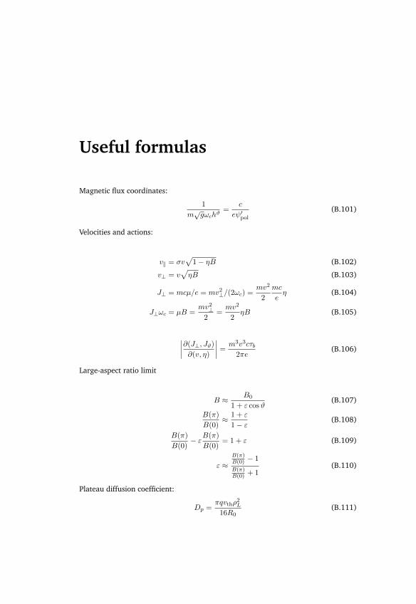
Useful formulas

Magnetic flux coordinates:

1

m√gωchϑ

=c

eψ′pol

(B.101)

Velocities and actions:

v‖ = σv√

1− ηB (B.102)

v⊥ = v√ηB (B.103)

J⊥ = mcµ/e = mv2⊥/(2ωc) =

mv2

2

mc

eη (B.104)

J⊥ωc = µB =mv2⊥

2=mv2

2ηB (B.105)

∣∣∣∣∂(J⊥, Jϑ)

∂(v, η)

∣∣∣∣ =m3v3cτb

2πe(B.106)

Large-aspect ratio limit

B ≈ B0

1 + ε cosϑ(B.107)

B(π)

B(0)≈ 1 + ε

1− ε (B.108)

B(π)

B(0)− εB(π)

B(0)= 1 + ε (B.109)

ε ≈B(π)B(0) − 1

B(π)B(0) + 1

(B.110)

Plateau diffusion coefficient:

Dp =πqvthρ

2L

16R0(B.111)


Ripple plateau diffusion coefficient:

Drp =

√πmϕq

2A2vthρ2L

4Rε2M (B.112)

List of Figures

1.1 Pendulum orbits in phase-space, energy dependence of bounce frequency 221.2 Contours of actions and angles for the pendulum . . . . . . . . . . . . . 231.3 Perturbation spectrum and non-linear bounce frequency for the pendulum 291.4 Pendulum orbits and energy dependence on perturbation amplitude . . 31

2.1 Airy functions and Scorer functions . . . . . . . . . . . . . . . . . . . . . 422.2 Action-dependent part of quasilinear dimensionless distribution function 432.3 Contours of quasilinear dimensionless distribution function . . . . . . . 432.4 Contours of non-linear dimensionless distribution function . . . . . . . 472.5 Numerical solution of dimensionless distribution function at θ = 0;π . . 482.6 Contours of numerical solution for dimensionless distribution function . 50

4.1 Attenuation factor depending on resonant diffusivity D . . . . . . . . . . 100

5.1 Superbanana plateau for RMPs, analytical validation, resonance . . . . . 1035.2 RMP: transport coefficients over Mach number, comparison NEO-2 . . . 1045.3 RMP: contributions to integral for transport coefficients. . . . . . . . . . 1055.4 Ripple: transport coefficients over Mach number, comparison NEO-2 . . 1065.5 RMP: influence of magnetic drift and shear on transport . . . . . . . . . 1065.6 AUG #30835: NTV torque from different models . . . . . . . . . . . . . 1095.7 AUG #30835: NTV torque from models with magnetic shear . . . . . . . 1105.8 Transport coefficient D11 at different non-linearities . . . . . . . . . . . 1115.9 Transport coefficient D11 dependency on perturbation amplitude . . . . 1115.10 Illustration of finite orbit width (poloidal projection) . . . . . . . . . . . 1135.11 Illustration of finite orbit width (error in approximation of ∆ϕ) . . . . . 114

Bibliography

SS Abdullaev and KH Finken. Hamiltonian guiding center equations in a toroidal system.Phys. Plasmas, 9(10):4193–4204, 2002.

CG Albert. Hamiltonian Theory of Resonant Transport Regimes in Tokamak Plasmas with Non-Axisymmetric Magnetic Perturbations. PhD thesis, TU Graz, Institute of Theoretical andComputational Physics, Petersgasse 16, 7 2017.

CG Albert and SV Kasilov. NEO-RT: Code for computing tokamak NTV torque in res-onant transport regimes. https://github.com/itpplasma/NEO-RT, 2017. accessed09/4/2020.

CG Albert, MF Heyn, G Kapper, SV Kasilov, W Kernbichler, and AF Martitsch. Evaluation oftoroidal torque by non-resonant magnetic perturbations in tokamaks for resonant trans-port regimes using a Hamiltonian approach. Phys. Plasmas, 23(8):082515, 2016a.

CG Albert, MF Heyn, G Kapper, SV Kasilov, W Kernbichler, and AF Martitsch. Hamilto-nian approach for evaluation of toroidal torque from finite amplitude non-axisymmetricperturbations of a tokamak magnetic field in resonant transport regimes. In 43rd EPSConference on Plasma Physics, page P1.051, 2016b.

CG Albert, MF Heyn, SV Kasilov, W Kernbichler, AF Martitsch, and AM Runov. Kineticmodeling of 3D equilibria in a tokamak. In J. Phys. Conf. Series, volume 775, page 012001.IOP Publishing, 2016c.

CG Albert, MF Heyn, SV Kasilov, W Kernbichler, and AF Martitsch. Finite orbit width effectson resonant transport regimes of neoclassical toroidal viscous torque within the Hamilto-nian approach. In 44th EPS Conference on Plasma Physics, page P1.182, 2017.

VI Arnold. Mathematical methods of classical mechanics, volume 60. Springer, 1989.

LA Artsimovich. Tokamak devices. Nuclear Fusion, 12(2):215, 1972.

A Bécoulet, DJ Gambier, and A Samain. Hamiltonian theory of the ion cyclotron minorityheating dynamics in tokamak plasmas. Physics of Fluids B: Plasma Physics, 3(1):137–150,1991.

AH Boozer. Enhanced transport in tokamaks due to toroidal ripple. Phys. Fluids, 23(11):2283–2290, 1980.

https://github.com/itpplasma/NEO-RT

142 BIBLIOGRAPHY

AH Boozer. Physics of magnetically confined plasmas. Rev. Mod. Phys., 76(4):1071, 2005.

AH Boozer. Perturbation to the magnetic field strength. Phys. Plasmas, 13(4):044501, 2006.

AJ Brizard. Jacobi zeta function and action-angle coordinates for the pendulum. Com-mun. Nonlin. Sci. Numer. Simul., 18(3):511–518, 2013.

BV Chirikov. Resonance processes in magnetic traps. J. Nuclear Energy C, 1(4):253, 1960.

BV Chirikov. A universal instability of many-dimensional oscillator systems. Phys. Rep., 52(5):263–379, 1979.

WD D’haeseleer, WNG Hitchon, JD Callen, and JL Shohet. Flux coordinates and magnetic fieldstructure. Springer Series in Computational Physics. Springer Berlin Heidelberg, 1991.

YN Dnestrovskii and DP Kostomarov. Numerical simulation of plasmas. Springer, 2012.

IG Eriksson and P Helander. Finite orbit width effects on stochastic ripple diffusion. Nuclearfusion, 33(5):767, 1993.

LG Eriksson and P Helander. Monte Carlo operators for orbit-averaged Fokker–Planck equa-tions. Phys. Plasmas, 1(2):308–314, 1994.

TE Evans, RA Moyer, PR Thomas, JG Watkins, TH Osborne, JA Boedo, EJ Doyle, ME Fen-stermacher, KH Finken, RJ Groebner, et al. Suppression of large edge-localized modes inhigh-confinement DIII-D plasmas with a stochastic magnetic boundary. Phys. Rev. Lett.,92(23):235003, 2004.

A Gil, J Segura, and NM Temme. Numerical methods for special functions. SIAM, 2007.

H Goldstein. Classical mechanics. Addison-Wesley, 2nd ed. edition, 1980.

IS Gradshtein and IM Ryzhik. Table of integrals, series, and products. 1965.

RD Hazeltine and AA Ware. The drift kinetic equation for toroidal plasmas with large massvelocities. Plasma Physics, 20(7):673, 1978.

RD Hazeltine, SM Mahajan, and DA Hitchcock. Quasi-linear diffusion and radial transportin tokamaks. Phys. Fluids, 24(6):1164–1179, 1981.

P Helander and DJ Sigmar. Collisional transport in magnetized plasmas, volume 4. CambridgeUniversity Press, 2005.

MF Heyn, IB Ivanov, SV Kasilov, W Kernbichler, I Joseph, A Moyer, and AM Runov. Kineticestimate of the shielding of resonant magnetic field perturbations by the plasma in DIII-D.Nuclear Fusion, 48:024005, 2008.

FL Hinton and RD Hazeltine. Theory of plasma transport in toroidal confinement systems.Rev. Mod. Phys., 48(2):239, 1976.

BIBLIOGRAPHY 143

SP Hirshman. The ambipolarity paradox in toroidal diffusion, revisited. Nuclear Fusion, 18(7):917, 1978.

SP Hirshman and DJ Sigmar. Neoclassical transport of impurities in tokamak plasmas. Nuc-lear Fusion, 21(9):1079, 1981.

K Ida and JC Rice. Rotation and momentum transport in tokamaks and helical systems.Nuclear Fusion, 54(4):045001, 2014.

SV Kasilov, AI Pyatak, and KN Stepanov. Nonlocal theory of cyclotron and cerenkov absorp-tion in nonuniformly magnetized plasma. Rev. Plasma Physics, 20:61, 1997.

SV Kasilov, W Kernbichler, AF Martitsch, H Maassberg, and MF Heyn. Evaluation of thetoroidal torque driven by external non-resonant non-axisymmetric magnetic field per-turbations in a tokamak. Phys. Plasmas, 21(9):092506, 2014.

AN Kaufman. Quasilinear diffusion of an axisymmetric toroidal plasma. Phys. Fluids, 15(6):1063–1069, 1972.

M Keilhacker, A Gibson, C Gormezano, PJ Lomas, PR Thomas, ML Watkins, P Andrew,B Balet, D Borba, CD Challis, et al. High fusion performance from deuterium-tritiumplasmas in jet. Nuclear Fusion, 39(2):209, 1999.

W Kernbichler, SV Kasilov, G Kapper, AF Martitsch, VV Nemov, C Albert, and MF Heyn.Solution of drift kinetic equation in stellarators and tokamaks with broken symmetryusing the code NEO-2. Plasma Phys. Contr. Fusion, 58(10):104001, 2016.

Ya I Kolesnichenko, VV Lutsenko, RB White, and Yu V Yakovenko. Theory of resonanceinfluence of sawtooth crashes on ions with large orbit width. Phys. Plasmas, 5(8):2963–2976, 1998.

Ya I Kolesnichenko, RB White, and Yu V Yakovenko. Precession of toroidally passing particlesin tokamaks and spherical tori. Phys. Plasmas, 10(5):1449–1457, 2003.

HA Kramers. Brownian motion in a field of force and the diffusion model of chemicalreactions. Physica, 7(4):284–304, 1940.

LD Landau and EM Lifshitz. Course of theoretical physics: Mechanics. Pergamon Press, 1960.

M Landreman, HM Smith, A Mollén, and P Helander. Comparison of particle trajectories andcollision operators for collisional transport in nonaxisymmetric plasmas. Phys. Plasmas,21(4):042503, 2014.

JD Lawson. Some criteria for a power producing thermonuclear reactor. Proc. Phys. Society.Section B, 70(1):6, 1957.

M Li, BN Breizman, and L Zheng. Canonical straight field line magnetic flux coordinates fortokamaks. J. Comp. Phys., 326:334–341, 2016.

AJ Lichtenberg and MA Lieberman. Regular and Chaotic Dynamics. Springer, 1983.

144 BIBLIOGRAPHY

RG Littlejohn. Variational principles of guiding centre motion. J. Plasma Phys., 29:111–125,2 1983.

A Loarte, G Saibene, R Sartori, D Campbell, M Becoulet, L Horton, T Eich, A Herrmann,G Matthews, N Asakura, et al. Characteristics of type i ELM energy and particle losses inexisting devices and their extrapolation to ITER. Plasma Phys. Contr. Fusion, 45(9):1549,2003.

SM Mahajan, RD Hazeltine, and DA Hitchcock. Quasilinear momentum and energy trans-port. Phys. Fluids, 26(3):700–704, 1983.

AF Martitsch, SV Kasilov, W Kernbichler, G Kapper, CG Albert, MF Heyn, HM Smith, E Strum-berger, S Fietz, W Suttrop, et al. Effect of 3d magnetic perturbations on the plasmarotation in asdex upgrade. Plasma Phys. Contr. Fusion, 58(7):074007, 2016.

JD Meiss and RD Hazeltine. Canonical coordinates for guiding center particles. Phys. Flu-ids B, 2(11):2563–2567, 1990.

VV Nemov, SV Kasilov, W Kernbichler, and MF Heyn. Evaluation of 1/ν neoclassical transportin stellarators. Phys. Plasmas, 6(12):4622–4632, 1999.

DR Nicholson. Introduction to plasma theory. Cambridge Univ Press, 1983.

J Nuckolls and L Wood. Laser compression of matter to super-high densities: thermonuclear(ctr) applications. Nature, 239:139, 1972.

J Ongena, R Koch, R Wolf, and H Zohm. Magnetic-confinement fusion. Nature Physics, 12(5):398–410, 2016.

MV Osipenko and RV Shurygin. Quasilinear hydrodynamics of trapped and flight particlesduring the alfven hf heating. Fiz. Plazmy, 15(11):1353–1367, 1989.

MV Osipenko and RV Shurygin. Radial transport of circulating and trapped ions during icrheating in a tokamak. Fiz. Plazmy, 16(12):1425–1436, 1990.

JK Park, AH Boozer, and JE Menard. Nonambipolar transport by trapped particles in toka-maks. Phys. Rev. Lett., 102:065002, Feb 2009.

Yu A Romanov and GF Filippov. Interaction of fast electron beams with longitudinal plasmawaves. Sov. Phys. JETP, 13:87–92, 1961.

S Satake, JK Park, H Sugama, and R Kanno. Neoclassical toroidal viscosity calculations intokamaks using a δf Monte Carlo simulation and their verifications. Phys. Rev. Letters,107(5):055001, 2011.

KC Shaing. Plasma flows and radial electric field in nonaxisymmetric toroidal plasmas.Phys. Fluids, 29(7):2231–2234, 1986.

KC Shaing. Poloidal and parallel plasma viscosities in tokamak geometry. Phys. Fluids B, 2(11):2847–2849, 1990.

BIBLIOGRAPHY 145

KC Shaing. Superbanana and superbanana plateau transport in finite aspect ratio tokamakswith broken symmetry. J. Plasma Phys., 81:905810203, 4 2015.

KC Shaing and JD Callen. Neoclassical flows and transport in nonaxisymmetric toroidalplasmas. Phys. Fluids, 26(11):3315–3326, 1983.

KC Shaing and SA Sabbagh. Neoclassical toroidal plasma viscosity with effects of finitebanana width for finite aspect ratio tokamaks. Physics of Plasmas, 23(7):072511, 2016.

KC Shaing and DA Spong. Extending the collisional fluid equations into the long mean-free-path regime in toroidal plasmas. i. plasma viscosity. Phys. Fluids B, 2(6):1190–1194,1990.

KC Shaing, MS Chu, and SA Sabbagh. Eulerian approach to bounce-transit and drift reson-ance and neoclassical toroidal plasma viscosity in tokamaks. Plasma Phys. Contr. Fusion,51(7):075015, 2009a.

KC Shaing, SA Sabbagh, and MS Chu. Neoclassical toroidal plasma viscosity in the superb-anana plateau regime for tokamaks. Plasma Phys. Contr. Fusion, 51(3):035009, 2009b.

KC Shaing, SA Sabbagh, and MS Chu. An approximate analytic expression for neoclassicaltoroidal plasma viscosity in tokamaks. Nuclear Fusion, 50(2):025022, 2010.

KC Shaing, K Ida, and SA Sabbagh. Neoclassical plasma viscosity and transport processes innon-axisymmetric tori. Nuclear Fusion, 55(12):125001, 2015.

H Smith. private communication.

L Spitzer. The stellarator concept. Phys. Fluids, 1(4):253–264, 1958.

Y Sun, Y Liang, KC Shaing, HR Koslowski, C Wiegmann, and T Zhang. Neoclassical toroidalplasma viscosity torque in collisionless regimes in tokamaks. Phys. Rev. Letters, 105(14):145002, 2010.

JB Taylor. Equilibrium and stability of plasma in arbitrary mirror fields. Phys. Fluids, 7(6):767–773, 1964.

AV Timofeev and MD Tokman. Quasi-linear equation for electron cyclotron resonance in-teraction with monochromatic radiation in magnetic traps. Plasma Phys. Rep., 20(4):336–340, 1994.

GE Uhlenbeck and LS Ornstein. On the theory of the Brownian motion. Phys. Rev., 36(5):823, 1930.

NG Van Kampen. Stochastic processes in physics and chemistry. AIP, 1983.

AA Vedenov, EP Velikhov, and RZ Sagdeev. Nonlinear oscillations of rarified plasma. NuclearFusion, 1(2):82, 1961.

146 BIBLIOGRAPHY

F Wagner, G Fussmann, T Grave, M Keilhacker, M Kornherr, K Lackner, K McCormick,ER Müller, A Stäbler, G Becker, et al. Development of an edge transport barrier at theh-mode transition of ASDEX. Physical Review Letters, 53(15):1453, 1984.

J Wesson. Tokamaks, volume 149. Oxford University Press, 2011.

RB White. Canonical Hamiltonian guiding center variables. Phys. Fluids B, 2(4):845–847,1990.

RB White and MS Chance. Hamiltonian guiding center drift orbit calculation for plasmas ofarbitrary cross section. Phys. Fluids, 27(10):2455–2467, 1984.

RB White, AH Boozer, and R Hay. Drift Hamiltonian in magnetic coordinates. Phys. Fluids,25(3):575–576, 1982.

VE Zakharov and VI Karpman. On the nonlinear theory of the damping of plasma waves.Sov. Phys. JETP, 16:351, 1963.

H Zohm. Edge localized modes (ELMs). Plasma Phys. Contr. Fusion, 38(2):105, 1996.


Vol. 1 Steffen Alvermann Effective Viscoelastic Behavior

of Cellular Auxetic Materials 2008 ISBN 978-3-902465-92-4

Vol. 2 Sendy Fransiscus Tantono

The Mechanical Behaviour of a Soilbag under Vertical Compression 2008 ISBN 978-3-902465-97-9

Vol. 3 Thomas Rüberg

Non-conforming FEM/BEM Coupling in Time Domain 2008 ISBN 978-3-902465-98-6

Vol. 4 Dimitrios E. Kiousis

Biomechanical and Computational Modeling of Atherosclerotic Arteries 2008 ISBN 978-3-85125-023-7

Vol. 5 Lars Kielhorn

A Time-Domain Symmetric Galerkin BEM for Viscoelastodynamics 2009 ISBN 978-3-85125-042-8

Vol. 6 Gerhard Unger Analysis of Boundary Element Methods

for Laplacian Eigenvalue Problems 2009 ISBN 978-3-85125-081-7


Vol. 7 Gerhard Sommer Mechanical Properties of Healthy and Diseased

Human Arteries 2010 ISBN 978-3-85125-111-1

Vol. 8 Mathias Nenning Infinite Elements for

Elasto- and Poroelastodynamics 2010 ISBN 978-3-85125-130-2

Vol. 9 Thanh Xuan Phan Boundary Element Methods for

Boundary Control Problems 2011 ISBN 978-3-85125-149-4

Vol. 10 Loris Nagler Simulation of Sound Transmission through

Poroelastic Plate-like Structures 2011 ISBN 978-3-85125-153-1

Vol. 11 Markus Windisch

Boundary Element Tearing and Interconnecting Methods for Acoustic and Electromagnetic Scattering 2011 ISBN 978-3-85125-152-4

Vol. 12 Christian Walchshofer

Analysis of the Dynamics at the Base of a Lifted Strongly Buoyant Jet Flame Using Direct Numerical Simulation 2011 ISBN 978-3-85125-185-2


Vol. 13 Matthias Messner Fast Boundary Element Methods in Acoustics

2012 ISBN 978-3-85125-202-6

Vol. 14 Peter Urthaler

Analysis of Boundary Element Methods for Wave Propagation in Porous Media 2012 ISBN 978-3-85125-216-3

Vol. 15 Peng Li

Boundary Element Method for Wave Propagation in Partially Saturated Poroelastic Continua 2012 ISBN 978-3-85125-236-1

Vol. 16 Andreas Jörg Schriefl

Quantification of Collagen Fiber Morphologies in Human Arterial Walls 2013 ISBN 978-3-85125-238-5

Vol. 17 Thomas S. E. Eriksson

Cardiovascular Mechanics 2013 ISBN 978-3-85125-277-4

Vol. 18 Jianhua Tong

Biomechanics of Abdominal Aortic Aneurysms 2013 ISBN 978-3-85125-279-8


Vol. 19 Jonathan Rohleder Titchmarsh–Weyl Theory and Inverse Problems

for Elliptic Differential Operators 2013 ISBN 978-3-85125-283-5

Vol. 20 Martin Neumüller

Space-Time Methods 2013 ISBN 978-3-85125-290-3

Vol. 21 Michael J. Unterberger

Microstructurally-Motivated Constitutive Modeling of Cross-Linked Filamentous Actin Networks 2013 ISBN 978-3-85125-303-0

Vol. 22 Vladimir Lotoreichik

Singular Values and Trace Formulae for Resolvent Power Differences of Self-Adjoint Elliptic Operators 2013 ISBN 978-3-85125-304-7

Vol. 23 Michael Meßner

A Fast Multipole Galerkin Boundary Element Method for the Transient Heat Equation 2014 ISBN 978-3-85125-350-4

Vol. 24 Lorenz Johannes John

Optimal Boundary Control in Energy Spaces 2014 ISBN 978-3-85125-373-3


Vol. 25 Hannah Weisbecker Softening and Damage Behavior of Human Arteries

2014 ISBN 978-3-85125-370-2

Vol. 26 Bernhard Kager

Efficient Convolution Quadrature based Boundary Element Formulation for Time-Domain Elastodynamics 2015 ISBN 978-3-85125-382-5

Vol. 27 Christoph M. Augustin

Classical and All-floating FETI Methods with Applications to Biomechanical Models 2015 ISBN 978-3-85125-418-1

Vol. 28 Elias Karabelas

Space-Time Discontinuous Galerkin Methods for Cardiac Electromechanics 2016 ISBN 978-3-85125-461-7

Vol. 29 Thomas Traub

A Kernel Interpolation Based Fast Multipole Method for Elastodynamic Problems 2016 ISBN 978-3-85125-465-5

Vol. 30 Matthias Gsell Mortar Domain Decomposition Methods for

Quasilinear Problems and Applications 2017 ISBN 978-3-85125-522-5


Vol. 31 Christian Kühn

Schrödinger operators and singular infinite rank perturbations 2017 ISBN 978-3-85125-551-5

Vol. 32 Michael H. Gfrerer

Vibro-Acoustic Simulation of Poroelastic Shell Structures 2018 ISBN 978-3-85125-573-7

Vol. 33 Markus Holzmann

Spectral Analysis of Transmission and Boundary Value Problems for Dirac Operators 2018 ISBN 978-3-85125-642-0

Vol. 34 Osman Gültekin

Computational Inelasticity of Fibrous Biological Tissues with a Focus on Viscoelasticity, Damage and Rupture 2019 ISBN 978-3-85125-655-0

Vol. 35 Justyna Anna Niestrawska

Experimental and Computational Analyses of Pathological Soft Tissues – Towards a Better Understanding of the Pathogenesis of AAA 2019 ISBN 978-3-85125-678-9


Vol. 36 Marco Zank

Inf-Sup Stable Space-Time Methods for Time-Dependent Partial Differential Equations 2020 ISBN 978-3-85125-721-2

Vol. 37 Christoph Irrenfried

Convective turbulent near wall heat transfer at high Prandtl numbers 2020 ISBN 978-3-85125-724-3

Vol. 38 Christopher Albert

Hamiltonian Theory of Resonant Transport Regimes in Tokamaks with Perturbed Axisymmetry 2020 ISBN 978-3-85125-746-5

hamiltonian approach to resonant transport regimes due to

Documents