haar measure on a locally compact quantum groupkahngb/research/papjrms.pdf · haar measure on a...
TRANSCRIPT
J. Ramanujan Math. Soc.18,No.4 (2003) 1–30
Haar measure on a locally compact quantum group∗
Byung-Jay KahngDepartment of Mathematics, University of Kansas, Lawrence, KS 66045e-mail: [email protected]
Communicated by: V. Kumar Murty
Received: July 15, 2003
Abstract. In the general theory of locally compact quantum groups, thenotion of Haar measure (Haar weight) plays the most significant role. Theaim of this paper is to carry out a careful analysis regarding Haar weight,in relation to general theory, for the specific non-compact quantum group(A,1) constructed earlier by the author. In this way, one can show that(A,1) is indeed a “(C∗-algebraic) locally compact quantum group” inthe sense of the recently developed definition given by Kustermans andVaes. Attention will be given to pointing out the relationship betweenthe original construction (obtained by deformation quantization) and thestructure maps suggested by general theory.
2000 Mathematics Subject Classification: 46L65, 46L51, 81R50
0. Introduction
According to the widely accepted paradigm (which goes back to Gelfandand Naimark in the 1940’s and has been reaffirmed by Connes and hisnon-commutative geometry program [5]) thatC∗-algebras are quantized/non-commutative locally compact spaces, theC∗-algebra framework is the mostnatural one in which to formulate a theory oflocally compact quantumgroups. There have been several examples ofC
∗-algebraic quantum groupsconstructed, beginning with Woronowicz’s (compact) quantumSU(2) group[25]. The examples of non-compactC∗-algebraic quantum groups have beenrather scarce, but significant progress has been made over the past decade.
Among the examples of non-compact type is the HopfC
∗-algebra(A,1)constructed by the author [8]. The construction is done by the method ofdeformation quantization, and the approach is a slight generalization of the one
∗The author wishes to thank Professor George Elliott, for his kind and helpfulcomments on the early draft of this paper.
1

2 Byung-Jay Kahng
used in Rieffel’s example of a solvable quantum group [19]. In fact,(A,1)
may be regarded as a “quantizedC∗
(H)” or a “quantizedC0(G)”, whereH isa Heisenberg-type Lie group andG is a certain solvable Lie group carrying anon-linear Poisson structure.
Motivation for choosing suitable comultiplication, counit, antipode (coin-verse), and Haar weight on(A,1) comes from the information at the levelof Poisson–Lie groups. The proofs were given by introducing some tools likethe multiplicative unitary operator. In this way, we could argue that(A,1),together with its additional structure maps, should be an example of anon-compact quantum group.
We further went on to find a “quantum universalR-matrix” type operatorrelated with(A,1) and studied its representation theory, indicating that the∗-representations ofA satisfy an interesting “quasitriangular” type property. See[8] and [9] (More discussion on the representation theory is given in [10].).
However, even with these strong indications suggested by our constructionand the representation theoretic applications, we did not quite make it clearwhether(A,1) actually is a locally compact (C∗-algebraic) quantum group.For instance, in [8], the discussion about the Haar weight on(A,1) wasrather incomplete, since we restricted our discussion to the level of a densesubalgebra of theC∗-algebraA. Even for the (simpler) example of Rieffel’s[19], the full construction of its Haar weight was not carried out. The problemof tying together these loose ends and establishing(A,1) as a locally compactquantum group in a suitable sense was postponed to a later occasion.
Part of the reason for the postponement was due to the fact that at thetime of writing, the question of the correct definition of a locally compactquantum group had not yet been settled. It was known that simply requiringthe existence of a counit and an antipode on the “locally compact quantumsemigroup”(A,1) is not enough. Some proposals had been made, but theywere at a rather primitive stage. Recently, the situation has improved: A newpaper by Kustermans and Vaes [14] appeared, in which they give a relativelysimple definition of a (reduced)C∗-algebraic quantum group.
In this new definition, the existence of a left invariant (Haar) weight anda right invariant weight plays the central role. In particular, they do not haveto include the existence of the antipode and its polar decomposition in theiraxioms. Unlike the axiom sets of Masuda and Nakagami [15], or those forKac algebras [6], which are either too complicated or too restrictive, theseproperties and others can be proved from the defining axioms. We are still farfrom achieving the goal of formulating a set of axioms in which we do not haveto invoke the existence of Haar measure. Considering this, it seems that thedefinition of Kustermans and Vaes is the most reasonable choice at this moment.
Now that we have an acceptable definition, we are going to return to ourexample(A,1) and verify that(A,1) is indeed a locally compact quantum

Haar measure on a locally compact quantum group 3
group. Our discussion will begin in Section 1 by describing the definition ofKustermans and Vaes, making precise the notion of a “C
∗-algebraic locallycompact quantum group”.
In section 2, we summarize a few results about our specific example(A,1).Instead of repeating our construction carried out in [8], we take a more econom-ical approach of describing results by relying less on the Poisson geometricaspects.
In section 3, which is the main part of this paper, we describe the Haarweight for(A,1) and make the notion valid in theC∗-algebra setting. Havingthe correct left/right invariant weights enables us to conclude that(A,1) isindeed a non-compactC∗-algebraic quantum group. We are benefiting a lotfrom being able to work with our specific example having a tracial weight, butmany of the techniques being used here are not necessarily type-specific, andtherefore, will be also useful in more general cases: Our discussion on the leftinvariance of Haar measure is strongly motivated by the new and attractiveapproach of Van Daele [23], [24].
In Sections 4 and 5, we say a little about the antipode and the modular func-tion of (A,1). By comparing our original definitions (motivated by Poisson–Lie group data) with the ones suggested by the general theory, we wish to givesome additional perspectives on these maps.
For the discussion to be complete, we need a description of the dual coun-terpart to(A,1). We included a very brief discussion of( ˆ
A,
ˆ
1) at the end ofSection 2, and also added a short Appendix (Section 6). For a more carefuldiscussion on the dual, see [11]. Meanwhile, we plan to pursue in our futurepapers the discussion on the quantum double, as well as the research on theduality of quantum groups in relation to the Poisson duality at the level of theirclassical limit.
As a final remark, we point out that while our original construction of(A,1) was by deformation quantization of Poisson–Lie groups, it can be alsoapproached algebraically using the recent framework of “twisted bicrossedproducts” of Vaes and Vainerman [22]. While we do believe in the advantageof the more constructive approach we took in [8] motivated by Poisson–Liegroups (especially in applications involving quantizations or representationtheory, as in [9], [10]), complementing it with the more theoretical approachpresented here will make our understanding more comprehensive.
1. Definitions, terminologies, and conventions
1.1 Weights onC∗-algebras
We will begin by briefly reviewing the theory of weights onC∗-algebras. Thepurpose is to make clear the notations used in the main definition of aC
∗-

4 Byung-Jay Kahng
algebraic quantum group (Definition 1.2) and in the proofs in later sections.For a more complete treatment and for standard terminologies on weights,refer to [3]. For instance, recall the standard notations likeN
ϕ
, Mϕ
, Mϕ
+, . . .associated to a weightϕ (on aC∗-algebraA). That is,
• N
ϕ
= {a ∈ A : ϕ(a∗
a) < ∞}
• M
ϕ
+
= {a ∈ A
+ : ϕ(a) < ∞}
• M
ϕ
= N
∗
ϕ
N
ϕ
The weights we will be considering are “proper weights”: A proper weightis a non-zero, densely defined weight on aC∗-algebra, which is lower semi-continuous [14].
If we are given a (proper) weightϕ on aC∗-algebra, we can define the setsF
ϕ
andG
ϕ
by
F
ϕ
= {ω ∈ A
∗
+
: ω(x) ≤ ϕ(x), ∀x ∈ A
+
}
G
ϕ
= {αω : ω ∈ F
ϕ
, α ∈ (0, 1)} ⊆ F
ϕ
.
HereA∗ denotes the norm dual ofA.These sets have been introduced by Combes, and they play a significant
role in the theory of weights. Note that onFϕ
, one can give a natural orderinherited fromA∗
+
. Meanwhile,Gϕ
is a directed subset ofFϕ
. That is, for everyω1, ω2 ∈ G
ϕ
, there exists an elementω ∈ G
ϕ
such thatω1, ω2 ≤ ω. Becauseof this,G
ϕ
is often used as an index set (of a net). For a proper weightϕ, wewould have:ϕ(x) = lim(ω(x))
ω∈G
ϕ
, for x ∈ A
+.By standard theory, for a weightϕ on aC∗-algebraA, one can associate to it
a “GNS-construction”(Hϕ
, π
ϕ
,3
ϕ
). Here,Hϕ
is a Hilbert space,3ϕ
: N
ϕ
→
H
ϕ
is a linear map such that3ϕ
(N
ϕ
) is dense inHϕ
and〈3
ϕ
(a),3
ϕ
(b)〉 =
ϕ(b
∗
a) for a, b ∈ N
ϕ
, andπϕ
is a representation ofA on H
ϕ
defined byπ
ϕ
(a)3
ϕ
(b) = 3
ϕ
(ab) for a ∈ A, b ∈ N
ϕ
. The GNS-construction is uniqueup to a unitary transformation.
If ϕ is proper, thenNϕ
is dense inA and3ϕ
: N
ϕ
→ H
ϕ
is a closed map.Alsoπ
ϕ
: A → B(H
ϕ
) is a non-degenerate∗-homomorphism. It is not difficultto show thatϕ has a natural extension to a weight onM(A), which we willstill denote byϕ. Meanwhile, since we can define for everyω ∈ G
ϕ
a uniqueelementω ∈ π
ϕ
(A)
′′
∗
such thatω ◦ π
ϕ
= ω, we can define a weightϕ on thevon Neumann algebraπ
ϕ
(A)
′′ in the following way:ϕ(x) = lim(ω(x))ω∈G
ϕ
,for x ∈ (π
ϕ
(A)
′′
)
+. Then, by standard terminology [21],ϕ is a “normal”,“semi-finite” weight on the von Neumann algebraπ
ϕ
(A)
′′.Motivated by the properties of normal, semi-finite weights on von Neumann
algebras, and to give somewhat of a control over the non-commutativity ofA,one introduces the notion of “KMS weights” [12]. The notion as defined belowis slightly different from (but equivalent to) the original one given by Combesin [4].
Haar measure on a locally compact quantum group 5
Definition 1.1. A proper weightϕ is called a “KMS weight” if there existsa norm-continuous one-parameter group of automorphismsσ ofA such that
(1) ϕ ◦ σ
t
= ϕ, for all t ∈ R.(2) ϕ(a∗
a) = ϕ(σ
i/2(a)σi/2(a)∗
), for all a ∈ D(σ
i/2).
Hereσi/2 is the analytic extension of the one-parameter groupσ
t
to i
2.
The one-parameter groupσ is called the “modular automorphism group” forϕ. It is uniquely determined whenϕ is faithful. Meanwhile, a proper weightϕ issaid to be “approximately KMS” if the associated (normal, semi-finite) weightϕ is faithful. A KMS weight is approximately KMS. For more discussion onthese classes of weights, including the relationship between the conditionsabove and the usual KMS condition, see [12]. Finally, note that in the specialcase whenϕ is a trace (i. e.ϕ(a∗
a) = ϕ(aa
∗
), for a ∈ N
ϕ
), it is clear thatϕ isKMS. The modular automorphism group will be trivial (≡ Id).
1.2 Definition of a locally compact quantum group
LetA be aC∗-algebra. Suppose1 : A → M(A⊗ A) is a non-degenerate∗-homomorphism (Later,1 will be given certain conditions for it to become acomultiplication.). A proper weightϕ on(A,1)will be calledleft invariant, if
ϕ((ω ⊗ id)(1a)) = ω(1)ϕ(a), (1.1)
for all a ∈ M
ϕ
+ andω ∈ A
∗
+
. Similarly,ϕ is calledright invariant, if
ϕ((id ⊗ω)(1a)) = ω(1)ϕ(a). (1.2)
By ω(1), we mean‖ω‖. Note here that we used the extensions ofϕ toM(A)in the equations, since we only know that(ω ⊗ id)(1a) ∈ M(A)
+. In thedefinition of locally compact quantum groups (to be given below), the “slices”of 1a will be assumed to be contained inA.
In the definitions above, the left [respectively, right] invariance conditionrequires the formula (1.1) to hold only fora ∈ M
ϕ
+. It is a very weak form ofleft invariance. In the case of locally compact quantum groups, the result canbe extended and a much stronger left invariance condition can be proved fromit. The proof is non-trivial. It was one of the important contributions made byKustermans and Vaes.
Next, let us state the definition of a locally compact (C
∗-algebraic) quantumgroup given by Kustermans and Vaes [14]. In the definition, [X] denotes theclosed linear span ofX.
Definition 1.2. Consider a C∗-algebra A and a non-degenerate∗-homomorphism1 : A → M(A⊗ A) such that

6 Byung-Jay Kahng
(1) (1⊗ id)1 = (id ⊗1)1
(2) [{(ω ⊗ id)(1a) : ω ∈ A
∗
, a ∈ A}] = A
(3) [{(id ⊗ω)(1a) : ω ∈ A
∗
, a ∈ A}] = A
Moreover, assume that there exist weightsϕ andψ such that
• ϕ is a faithful, left invariant approximate KMS weight on(A,1).• ψ is a right invariant approximate KMS weight on(A,1).
Then we say that(A,1) is a (reduced)C∗-algebraic quantum group.
First condition is the “coassociativity” condition for the “comultiplication”1. By the non-degeneracy, it can be naturally extended toM(A) [we canalso extend(1⊗ id) and(id ⊗1)], thereby making the expression valid. Thetwo density conditions more or less correspond to the cancellation propertyin the case of ordinary groups, although they are somewhat weaker. The lastaxiom corresponds to the existence of Haar measure (The weightsϕ andψactually turn out to be faithful KMS weights.). For more on this definition (e. g.discussions on how one can build other structure maps like the antipode), see[14].
2. The HopfC∗-algebra (A,1)
Our main object of study is the HopfC∗-algebra(A,1) constructed in[8]. As a C
∗-algebra,A is isomorphic to a twisted groupC∗-algebraC
∗
(H/Z,C0(g/q), σ ), whereH is the(2n+ 1)-dimensional Heisenberg Liegroup andZ is the center ofH . Whereas,g = h
∗ is the dual space of the Liealgebrah of H andq = z
⊥, for z ⊆ h corresponding toZ. SinceH is a nilpo-tent Lie group,H ∼
=
h andZ ∼
=
z, as vector spaces. We denoted byσ (notto be confused with the modular automorphism group) the twisting cocyclefor the groupH/Z. As constructed in [8],σ is a continuous field of cocyclesg/q 3 r 7→ σ
r , where
σ
r
((x, y), (x
′
, y
′
)) = e[ηλ
(r)β(x, y
′
)]. (2.1)
Following the notation of the previous paper, we used:e(t) = e
(−2πi)t andη
λ
(r) =
e
2λr−1
2λ , whereλ is a fixed real constant. We denote byβ( , ) the innerproduct. The elements(x, y), (x ′
, y
′
) are group elements inH/Z.In [8], we showed that theC∗-algebraA is a deformation quantization (in
Rieffel’s “strict” sense [18], [20]) ofC0(G), whereG is a certain solvable Liegroup which is thedual Poisson–Lie groupof H . The numberλ mentionedabove determines the group structure ofG (Whenλ = 0, the groupG becomesabelian, which is not very interesting.). See Definition 1.6 of [8] for the precisedefinition ofG. For convenience, we fixed the deformation parameter as~ = 1.This is the reason why we do not see it in the definition ofA. If we wish to

Haar measure on a locally compact quantum group 7
illustrate the deformation process, we may just replaceβ by~β, and let~ → 0.When~ = 0 (i. e. classical limit), we haveσ ≡ 1, and hence,A
~=0∼
=
C0(G).Throughout this paper, we will just work withA = A
~=1.Let us be a little more specific and recall some of the notations and results
obtained in [8], while referring the reader to that paper for more details on theconstruction of our main example(A,1).
We first introduce the subspaceA, which is a dense subspace ofA consistingof the functions inS3c(H/Z × g/q), the space of Schwartz functions in the(x, y, r) variables having compact support in ther(∈ g/q) variable. OnA, wedefine the (twisted) multiplication and the (twisted) involution as follows:
(f × g)(x, y, r) =
∫
f (x, y, r)g(x − x, y − y, r)
e[ηλ
(r)β(x, y − y)] dxdy, (2.2)
and
f
∗
(x, y, r) = f (−x,−y, r)e[ηλ
(r)β(x, y)]. (2.3)
It is not difficult to see thatA = S3c(H/Z× g/q) is closed under the multipli-cation (2.2) and the involution (2.3). Here, we observe the role being playedby the twisting cocycleσ defined in (2.1).
Elements ofA are viewed as operators on the Hilbert spaceH = L
2(H/Z×
g/q), via the “regular representation”,L, defined by
(L
f
ξ)(x, y, r) =
∫
f (x, y, r)ξ(x − x, y − y, r)e[ηλ
(r)β(x, y − y)] dxdy.
(2.4)
For f ∈ A, define its norm by‖f ‖ = ‖L
f
‖. Then (A,×, ∗
, ‖ ‖) asabove is a pre-C∗-algebra, whose completion is theC∗-algebraA ∼
=
C
∗
(H/Z,C0(g/q), σ ).
Remark. To be more precise, the completion ofA with respect to the normgiven by the regular representation,L, should be isomorphic to the “reduced”twisted groupC∗-algebraC∗
r
(H/Z,C0(g/q), σ ). But by using a result ofPacker and Raeburn [17], it is rather easy to see that the amenability condi-tion holds in our case, thereby obtaining the isomorphism with the “full”C
∗-algebra as above. Meanwhile, we should point out that our definition ofA isslightly different from that of [8]: There,A is a subspace ofC0(G), while atpresent we view it as functions contained inC0(H/Z × g/q), in the(x, y, r)variables. Nevertheless, they can be regarded as the same since we consider thefunctions inA as operators contained in ourC∗-algebraA. The identificationof the function spaces is given by the (partial) Fourier transform.

8 Byung-Jay Kahng
TheC∗-algebraA becomes a HopfC∗-algebra, together with itscomultipli-cation1. In the following proposition, we chose to describe the comultiplica-tion in terms of a certain “multiplicative unitary operator”U
A
∈ B(H ⊗ H).See [8] for a discussion on the construction ofU
A
.
Proposition 2.1. (1) LetUA
be the operator onH ⊗ H defined by
U
A
ξ(x, y, r, x
′
, y
′
, r
′
) = (e
−λr
′
)
n
e[ηλ
(r
′
)β(e
−λr
′
x, y
′
− e
−λr
′
y)]
ξ(e
−λr
′
x, e
−λr
′
y, r+r
′
, x
′
−e
−λr
′
x, y
′
−e
−λr
′
y, r
′
).
ThenUA
is a unitary operator, and is multiplicative. That is,
U12U13U23 = U23U12.
(2) For f ∈ A, define1f by
1f = U
A
(f ⊗ 1)UA
∗
,
wheref and1f are understood as operatorsLf
and(L⊗ L)
1f
. Then1 can be extended to a non-degenerateC∗-homomorphism1 : A →
M(A⊗ A) satisfying the coassociativity condition:
(1⊗ id)(1f ) = (id ⊗1)(1f ).
Proof. See Proposition 3.1 and Theorem 3.2 of [8], together with theRemark 3.3 following them. 2
There is a useful characterization of theC∗-algebraA, via the multiplicativeunitary operatorU
A
. The following result is suggested by the general theoryon multiplicative unitaries by Baaj and Skandalis [2].
Proposition 2.2. LetUA
be as above. Consider the subspaceA(U
A
) ofB(H)defined below:
A(U
A
) = {(ω ⊗ id)(UA
) : ω ∈ B(H)
∗
}.
By standard theory,A(UA
) is a subalgebra of the operator algebraB(H), andthe subspaceA(U
A
)H forms a total set inH.We can show that the norm-closure inB(H) of the algebraA(U
A
) is exactlytheC∗-algebraA we are studying. That is,
A = {(ω ⊗ id)(UA
) : ω ∈ B(H)
∗
}
‖ ‖
.

Haar measure on a locally compact quantum group 9
Proof. The definition and the properties ofA(U
A
) can be found in [2]. Weonly need to verify the last statement. We will work with the standard notationω
ξ,η
, whereξ, η ∈ H. It is defined byωξ,η
(a) = 〈aξ, η〉, and it is well knownthat linear combinations of theω
ξ,η
are (norm) dense inB(H)∗
.So consider(ω
ξ,η
⊗ id)(UA
) ∈ B(H). We may further assume thatξ andηare continuous functions having compact support. Letζ ∈ H. Then, by usingchange of variables, we have:
(ω
ξ,η
⊗ id)(UA
)ζ(x, y, r)
=
∫
(U
A
(ξ ⊗ ζ ))(x, y, r; x, y, r)η(x, y, r) dxdydr
=
∫
f (x, y, r)ζ(x − x, y − y, r)e[ηλ
(r)β(x, y − y)] dxdy,
where
f (x, y, r) =
∫
ξ(x, y, r + r)(e
λr
)
n
η(e
λr
x, e
λr
y, r) dr.
Sinceξ and η areL2-functions, the integral (and thusf ) is well defined.Actually, sincef is essentially defined as a convolution product (inr) of twocontinuous functions having compact support,f will be also continuous withcompact support. This means that
(ω
ξ,η
⊗ id)(UA
) = L
f
∈ A.
Meanwhile, since the choice ofξ andη is arbitrary, we can see that the collec-tion of thef will form a total set in the space of continuous functions in the(x, y, r) variables having compact support. It follows from these two conclu-sions that
{(ω ⊗ id)(UA
) : ω ∈ B(H)
∗
}
‖ ‖
= A.
2
Meanwhile, from the proof of Theorem 3.2 of [8], we also have the followingresult. These are not same as the density conditions of Definition 1.2, but areactually stronger: This is rather well known and can be seen easily by applyinglinear functionals (Use the fact that anyω ∈ A
∗ has the formω′
(· b), withω
′
∈ A
∗ andb ∈ A.).
Proposition 2.3. We have:
(1) 1(A)(1 ⊗ A) is dense inA⊗ A.(2) 1(A)(A⊗ 1) is dense inA⊗ A.

10 Byung-Jay Kahng
Proof. In the proof of the non-degeneracy of1 in Theorem 3.2 and Remark 3.3of [8], we showed that the(1f )(1⊗ g)’s (for f, g ∈ A) form a total set in thespaceS3c(H/Z × g/q × H/Z × g/q), which is in turn shown to be dense inA⊗A: Under the natural injection fromS3c(H/Z × g/q ×H/Z × g/q) intoB(H⊗H), the algebraic tensor productA�A is sent into a dense subset of thealgebraic tensor productA�A. Since elements inS3c(H/Z×g/q×H/Z×g/q)
can be approximated (in theL1-norm) by elements ofA � A, we see thatS3c(H/Z×g/q×H/Z×g/q) is mapped into a dense subset (in theC
∗ norm)of A ⊗ A. Thus it follows that1(A)(1 ⊗ A) is dense inA ⊗ A. The secondstatement can be shown in exactly the same way. 2
Turning our attention to the other structures on(A,1), we point out that byviewingA as a “quantumC0(G)”, we can construct itscounit, ε, andantipode,S. These are described in the following proposition.
Proposition 2.4. (1) For f ∈ A, defineε : A → C by
ε(f ) =
∫
f (x, y,0) dxdy.
Thenε can be extended to aC∗-homomorphism fromA to C satisfyingthe condition:(id ⊗ε)1 = (ε ⊗ id)1 = id.
(2) Consider a mapS : A → A defined by
(S(f ))(x, y, r) = (e
2λr)
n
e[ηλ
(r)β(x, y)]f (−eλrx,−eλry,−r).
ThenS can be extended to an anti-automorphismS : A → A, satisfying:S(S(a)
∗
)
∗
= a and (S ⊗ S)(1a) = χ(1(S(a))), whereχ denotes theflip. Actually, we have:S2
= Id.
Proof. See Theorem 4.1 and Proposition 4.3 of [8]. We had to use partialFourier transform to convert these results into the level of functions in the(x, y, r) variables. We also mention here thatS is defined byS(a) =
ˆ
Ja
∗
ˆ
J ,where ˆ
J is an involutive operator onH defined by
ˆ
Jξ(x, y, r) = (e
λr
)
n
ξ(e
λr
x, e
λr
y,−r).
Since ˆ
J is an anti-unitary involutive operator, it is easy to see thatS is an anti-automorphism such thatS2
= Id. 2
Remark. The notation for the operatorˆJ is motivated by the modular theoryand by [15]. Meanwhile, since the square of the antipode is the identity, ourexample is essentially theKacC∗-algebra(Compare with [7], although ourexample is actually non-unimodular, unlike in that paper. See also [22], ofwhich our example is a kind of a special case.). We also note that in [8], we
Haar measure on a locally compact quantum group 11
usedκ to denote the antipode, while we useS here. This is done so that we canmatch our notation with the preferred notation of Kustermans and Vaes [14].
In general, the counit may as well be unbounded. So Proposition 2.4 impliesthat what we have is a more restrictive “bounded counit”. HavingS bounded isalso a bonus. Even so, the result of the proposition is not enough to legitimatelycall S an antipode. To give some support for our choice, we also showed thefollowing, albeit only at the level of the function spaceA. See section 4 of [8].
Proposition 2.5. For f ∈ A, we have:
m((id ⊗S)(1f )) = m((S ⊗ id)(1f )) = ε(f )1,
wherem : A ⊗ A → A is the multiplication.
This is the required condition for the antipode in the purely algebraic settingof Hopf algebra theory [16]. In this sense, the proposition gives us a modestjustification for our choice ofS. However, in the operator algebra setting, thisis not the correct way of approach. One of the serious obstacles is that themultiplicationm is in general not continuous for the operator norm, therebygiving us trouble extendingm toA⊗ A orM(A⊗ A).
Because of this and other reasons (including the obstacles due to possibleunboundedness ofε andS), one has to develop a new approach. Motivatedby the theory of Kac algebras [6], operator algebraists have been treatingthe antipode together with the notion of the Haar weight. This is also theapproach chosen by Masuda, Nakagami [15] and by Kustermans, Vaes [14].As we mentioned earlier in this paper, any rigorous discussion about locallycompact quantum groups should be built around the notion of Haar weights. Inthe next section, we will exclusively discuss the Haar weight for our(A,1),and establish that(A,1) is indeed a “C∗-algebraic locally compact quantumgroup”. We will come back to the discussion of the antipode in section 4.
Before wrapping up this section, let us mention the dual object for our(A,1), which would be the “dual locally compact quantum group”(
ˆ
A,
ˆ
1).Our discussion here is kept to a minimum. More careful discussion on(
ˆ
A,
ˆ
1)
is presented in a separate paper [11]. Meanwhile, see Appendix (Section 6) fora somewhat different characterization of the dual object.
Proposition 2.6. (1) LetUA
be as above. Consider the subspaceˆ
A(U
A
) ofB(H) defined by
ˆ
A(U
A
) = {(id ⊗ω)(U
A
) : ω ∈ B(H)
∗
}.
Then ˆ
A(U
A
) is a subalgebra of the operator algebraB(H), and the sub-space ˆ
A(U
A
)H forms a total set inH.
12 Byung-Jay Kahng
(2) The norm-closure inB(H) of the algebra ˆ
A(U
A
) is theC∗-algebra ˆ
A:
ˆ
A = {(id ⊗ω)(U
A
) : ω ∈ B(H)
∗
}
‖ ‖
.
(3) For b ∈
ˆ
A(U
A
), define ˆ
1b by ˆ
1b = U
A
∗
(1 ⊗ b)U
A
. Then ˆ
1 can beextended to the comultiplicationˆ1 : ˆ
A → M(
ˆ
A⊗
ˆ
A).(4) The duality exists at the level ofA(U
A
) and ˆ
A(U
A
), by the followingformula:
〈L(ω), ρ(ω
′
)〉 = (ω ⊗ ω
′
)(U
A
) = ω(ρ(ω
′
)) = ω
′
(L(ω)),
whereL(ω) = (ω ⊗ id)(UA
) ∈ A(U
A
) and ρ(ω′
) = (id ⊗ω
′
)(U
A
) ∈
ˆ
A(U
A
).
Proof. Since our multiplicative unitary operatorUA
is known to be regular,we can just follow the standard theory of multiplicative unitary operators [2].
2
At this moment,( ˆ
A,
ˆ
1) is just a quantum semigroup, having only the comul-tiplication. However, once we establish in section 3 the proof that our(A,1)
is indeed a (C∗-algebraic) locally compact quantum group, we can apply thegeneral theory [14], and show that( ˆ
A,
ˆ
1) is also a locally compact quantumgroup. Meanwhile, we can give a more specific description of theC
∗-algebraˆ
A, as presented below.
Proposition 2.7. Let ˆ
A be the space of Schwartz functions in the(x, y, r)variables having compact support in ther variable. Forf ∈
ˆ
A, define theoperatorρ
f
∈ B(H) by
(ρ
f
ζ )(x, y, r) =
∫
(e
λr
)
n
f (x, y, r)ζ(e
λr
x, e
λr
y, r − r) dr. (2.5)
Then theC∗-algebra ˆ
A is generated by the operatorsρf
.
Proof. As in the proof of Proposition 2.2, consider the operators(id ⊗ω
ξ,η
)(U
A
)
in ˆ
A(U
A
). Without loss of generality, we can assume thatξ andη are contin-uous functions having compact support. Letζ ∈ H. Then we have:
(id ⊗ω
ξ,η
)(U
A
)ζ(x, y, r)
=
∫
(U
A
(ζ ⊗ ξ))(x, y, r; x, y, r)η(x, y, r) dxdydr
=
∫
(e
λr
)
n
f (x, y, r)ζ(e
λr
x, e
λr
y, r − r) dr,

Haar measure on a locally compact quantum group 13
where
f (x, y, r) =
∫
e[ηλ
(r)β(x, y − e
−λr
y)]
ξ(x − e
λr
x, y − e
λr
y,−r)η(x, y,−r) dxdy.
We see that(id ⊗ω
ξ,η
)(U
A
) = ρ
f
, andf is continuous with compact support.By the same argument we used in the proof of Proposition 2.2, we concludethat theC∗-algebra generated by the operatorsρ
f
, f ∈
ˆ
A, coincides with theC
∗-algebra ˆ
A. 2
The above characterization ofˆA is useful when we wish to regardˆA as adeformation quantization of a Poisson–Lie group. Actually, by using partialFourier transform, we can show without difficulty thatˆ
A
∼
=
ρ(C
∗
(G)), whereρ is the right regular representation ofC∗
(G). In a future paper, we will havean occasion to discuss the duality between(A,1) and( ˆ
A,
ˆ
1) in relation tothe Poisson–Lie group duality betweenG andH .
3. Haar weight
We have been arguing that(A,1) is a “quantizedC0(G)”. This viewpointhas been helpful in our construction of its comultiplication1, counitε, andantipodeS.
To discuss the (left invariant) Haar weight on(A,1), we pull this viewpointonce more. Recall that the group structure onG has been specifically chosen(Definition 1.6 of [8]) so that the Lebesgue measure onG becomes its leftinvariant Haar measure. This suggests us to build the Haar weight on(A,1)
from the Lebesgue measure onG. At the level of functions inA, this suggestiontakes the following form:
Definition 3.1. OnA, define a linear functionalϕ by
ϕ(f ) =
∫
f (0, 0, r) dr.
In section 5 of [8], we obtained some results (including the “left invariance”property) indicating that our choice ofϕ is a correct one. However, the discus-sion was limited to the level of functions inA, and thus not very satisfactory.
Jumping up from the function level to the operator level can be quite techni-cal, and it is not necessarily an easy task (For example, see [1], [23].). Whereas,if one wants to rigorously formulate the construction of a locally compact quan-tum group in the operator algebra setting, this step of “jumping up” (extendingϕ to a weight) is very crucial.
Fortunately in our case, the discussion will be much simpler than some ofthe difficult examples, since we can show thatϕ is tracial. Note the following:
14 Byung-Jay Kahng
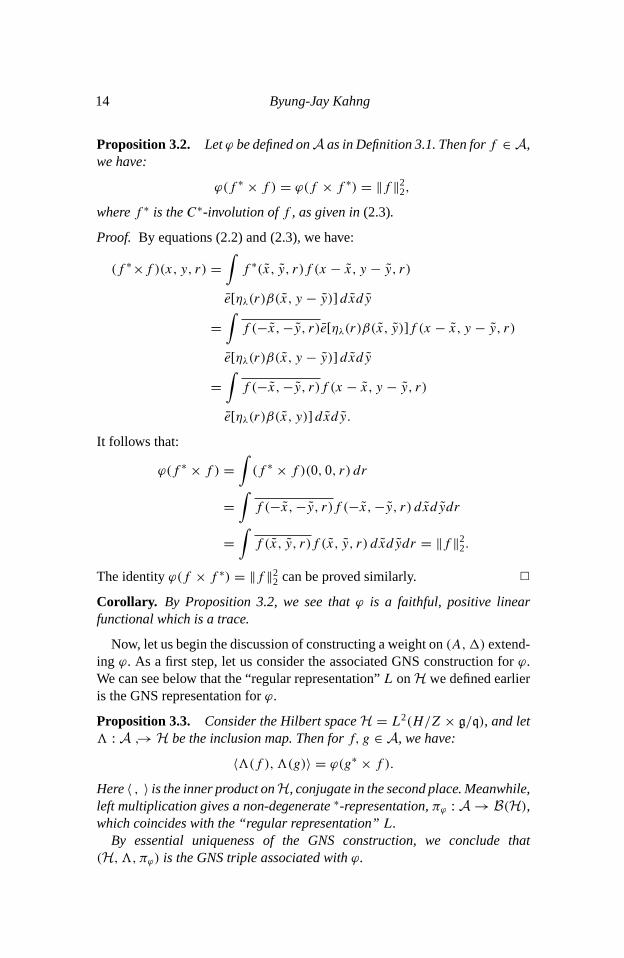
Proposition 3.2. Letϕ be defined onA as in Definition 3.1. Then forf ∈ A,we have:
ϕ(f
∗
× f ) = ϕ(f × f
∗
) = ‖f ‖
22,
wheref ∗ is theC∗-involution off , as given in(2.3).
Proof. By equations (2.2) and (2.3), we have:
(f
∗
×f )(x, y, r) =
∫
f
∗
(x, y, r)f (x − x, y − y, r)
e[ηλ
(r)β(x, y − y)] dxdy
=
∫
f (−x,−y, r)e[ηλ
(r)β(x, y)]f (x − x, y − y, r)
e[ηλ
(r)β(x, y − y)] dxdy
=
∫
f (−x,−y, r)f (x − x, y − y, r)
e[ηλ
(r)β(x, y)] dxdy.
It follows that:
ϕ(f
∗
× f ) =
∫
(f
∗
× f )(0, 0, r) dr
=
∫
f (−x,−y, r)f (−x,−y, r) dxdydr
=
∫
f (x, y, r)f (x, y, r) dxdydr = ‖f ‖
22.
The identityϕ(f × f
∗
) = ‖f ‖
22 can be proved similarly. 2
Corollary. By Proposition 3.2, we see thatϕ is a faithful, positive linearfunctional which is a trace.
Now, let us begin the discussion of constructing a weight on(A,1) extend-ing ϕ. As a first step, let us consider the associated GNS construction forϕ.We can see below that the “regular representation”L onH we defined earlieris the GNS representation forϕ.
Proposition 3.3. Consider the Hilbert spaceH = L
2(H/Z × g/q), and let
3 : A ↪→ H be the inclusion map. Then forf, g ∈ A, we have:
〈3(f ),3(g)〉 = ϕ(g
∗
× f ).
Here〈 , 〉 is the inner product onH, conjugate in the second place. Meanwhile,left multiplication gives a non-degenerate∗-representation,π
ϕ
: A → B(H),which coincides with the “regular representation”L.
By essential uniqueness of the GNS construction, we conclude that(H,3, π
ϕ
) is the GNS triple associated withϕ.

Haar measure on a locally compact quantum group 15
Proof. SinceA = S3c(H/Z × g/q), clearlyA is a dense subspace ofH. Theinclusion map (i. e.3(f ) = f ) carriesA into H. Now for f, g ∈ A,
ϕ(g
∗
× f ) =
∫
g
∗
(x, y, r)f (0 − x, 0 − y, r)e[ηλ
(r)β(x, 0 − y)] dxdydr
=
∫
g(−x,−y, r)e[ηλ
(r)β(x, y)]f (−x,−y, r)e[ηλ
(r)β(x,−y)] dxdydr
=
∫
g(x, y, r)f (x, y, r) dxdydr = 〈f, g〉 = 〈3(f ),3(g)〉.
Consider now the left-multiplication representationπϕ
. Then forf, ξ ∈ A,
(π
ϕ
(f ))(3(ξ))(x, y, r) := (3(f × ξ))(x, y, r) = (f × ξ)(x, y, r)
=
∫
f (x, y, r)ξ(x − x, y − y, r)
e[ηλ
(r)β(x, y − y)] dxdy
= L
f
ξ(x, y, r).
This shows thatπϕ
is just the∗-representationL of equation (2.4). Since
A = 3(A) is dense inH, it is also clear thatπϕ
(A)H
‖ ‖2= H, which means
thatπϕ
(= L) is non-degenerate. 2
We are ready to show thatA(⊆ H) is a “left Hilbert algebra” (See definitionbelow.).
Definition 3.4.([4], [21]) By a left Hilbert algebra, we mean an involutivealgebraU equipped with a scalar product such that the involution is an anti-linear preclosed mapping in the associated Hilbert spaceH and such thatthe left-multiplication representationπ of U is non-degenerate, bounded, andinvolutive.
Proposition 3.5. The algebraA, together with its inner product inheritedfrom that ofH, is a left Hilbert algebra.
Proof. We viewA = 3(A) ⊆ H. It is an involutive algebra equipped withthe inner product inherited from that ofH. Sinceϕ is a trace, the mapf 7→ f
∗
is not just closable, but it is actually isometry and hence bounded. Note thatfor everyf, g ∈ A, we have:
〈f
∗
, g〉 = ϕ(g
∗
× f
∗
) = ϕ(f
∗
× g
∗
) = 〈g
∗
, f 〉,
where we used the property thatϕ is a trace. The remaining conditions forA being a left Hilbert algebra are immediate consequences of the previousproposition. 2
16 Byung-Jay Kahng
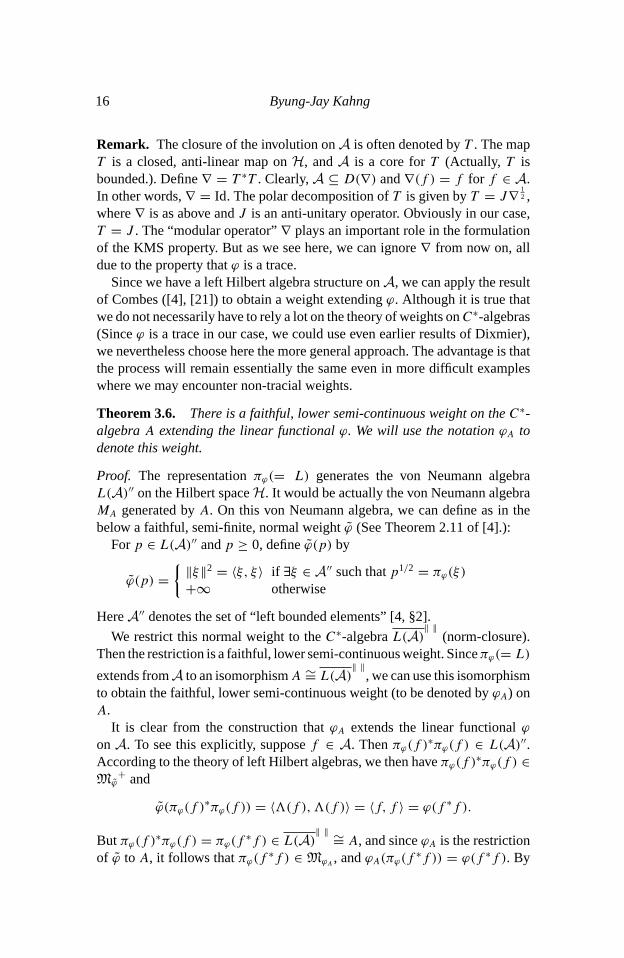
Remark. The closure of the involution onA is often denoted byT . The mapT is a closed, anti-linear map onH, andA is a core forT (Actually, T isbounded.). Define∇ = T
∗
T . Clearly,A ⊆ D(∇) and∇(f ) = f for f ∈ A.In other words,∇ = Id. The polar decomposition ofT is given byT = J∇
12 ,
where∇ is as above andJ is an anti-unitary operator. Obviously in our case,T = J . The “modular operator”∇ plays an important role in the formulationof the KMS property. But as we see here, we can ignore∇ from now on, alldue to the property thatϕ is a trace.
Since we have a left Hilbert algebra structure onA, we can apply the resultof Combes ([4], [21]) to obtain a weight extendingϕ. Although it is true thatwe do not necessarily have to rely a lot on the theory of weights onC
∗-algebras(Sinceϕ is a trace in our case, we could use even earlier results of Dixmier),we nevertheless choose here the more general approach. The advantage is thatthe process will remain essentially the same even in more difficult exampleswhere we may encounter non-tracial weights.
Theorem 3.6. There is a faithful, lower semi-continuous weight on theC
∗-algebraA extending the linear functionalϕ. We will use the notationϕ
A
todenote this weight.
Proof. The representationπϕ
(= L) generates the von Neumann algebraL(A)
′′ on the Hilbert spaceH. It would be actually the von Neumann algebraM
A
generated byA. On this von Neumann algebra, we can define as in thebelow a faithful, semi-finite, normal weightϕ (See Theorem 2.11 of [4].):
Forp ∈ L(A)
′′ andp ≥ 0, defineϕ(p) by
ϕ(p) =
{
‖ξ‖
2= 〈ξ, ξ〉 if ∃ξ ∈ A
′′ such thatp1/2= π
ϕ
(ξ)
+∞ otherwise
HereA
′′ denotes the set of “left bounded elements” [4, §2].
We restrict this normal weight to theC∗-algebraL(A)‖ ‖
(norm-closure).Then the restriction is a faithful, lower semi-continuous weight. Sinceπ
ϕ
(= L)
extends fromA to an isomorphismA ∼
=
L(A)
‖ ‖
, we can use this isomorphismto obtain the faithful, lower semi-continuous weight (to be denoted byϕ
A
) onA.
It is clear from the construction thatϕA
extends the linear functionalϕon A. To see this explicitly, supposef ∈ A. Thenπ
ϕ
(f )
∗
π
ϕ
(f ) ∈ L(A)
′′.According to the theory of left Hilbert algebras, we then haveπ
ϕ
(f )
∗
π
ϕ
(f ) ∈
M
ϕ
+ and
ϕ(π
ϕ
(f )
∗
π
ϕ
(f )) = 〈3(f ),3(f )〉 = 〈f, f 〉 = ϕ(f
∗
f ).
But πϕ
(f )
∗
π
ϕ
(f ) = π
ϕ
(f
∗
f ) ∈ L(A)
‖ ‖
∼
=
A, and sinceϕA
is the restrictionof ϕ toA, it follows thatπ
ϕ
(f
∗
f ) ∈ M
ϕ
A
, andϕA
(π
ϕ
(f
∗
f )) = ϕ(f
∗
f ). By
Haar measure on a locally compact quantum group 17
using polarization, we conclude that in general,L(A) ⊆ M
ϕ
A
and
ϕ
A
(π
ϕ
(f )) = ϕ(f ), ∀f ∈ A.
2
Remark. From the proof of the proposition, we can see thatϕ
A
is denselydefined (note that we haveL(A) ⊆ M
ϕ
A
). It is a faithful weight since the linearfunctionalϕ is faithful onA. Sinceϕ
A
is obtained by restricting the normalweightϕ on the von Neumann algebra level, it follows that it is also KMS (Wewill not give proof of this here, sinceϕ being a trace makes this last statementredundant: See comment after Definition 1.1.). In the terminology of the firstsection,ϕ
A
is a “proper” weight, which is “faithful” and “KMS” (actually atrace).
From now on, let us turn our attention to the weightϕ
A
. Consider the GNStriple associated withϕ
A
, given by the following ingredients:
• H
ϕ
A
= H
• 3
ϕ
A
: N
ϕ
A
→ H. The proof of the previous theorem suggests that fora ∈ N
ϕ
A
, there exists a unique “left bounded” elementv ∈ H. We define3
ϕ
A
(a) = v.• π
ϕ
A
: A → B(H) is the inclusion map.
Note that forf ∈ A, we have:3ϕ
A
(π
ϕ
(f )) = 3(f ). So we know that3ϕ
A
has a dense range inH.Define30 as the closure of the mappingL(A) → H : π
ϕ
(f ) 7→ 3(f ).Let us denote byA0 the domain of30. Clearly,30 is a restriction of3
ϕ
A
. Byusing the properties ofϕ
A
, including its lower semi-continuity and the “leftinvariance” at the level of the∗-algebraA, one can improve the left invarianceup to the level ofA0. One can also show thatA0 = N
ϕ
A
and thatL(A) is acore for3
ϕ
A
(We can more or less follow the discussion in section 6 of [13].).From these results, the left invariance ofϕ
A
can be proved at theC∗-algebralevel (A similar result can be found in Corollary 6.14 of [13].).
However, we plan to present a somewhat different proof of the left invari-ance, which is in the spirit of Van Daele’s recently developed method [23],[24]. The main strategy is to show that there exists a faithful, semi-finite, nor-mal weightµ on B(H) such that at least formally,µ(ba) = ϕ
B
(b)ϕ
A
(a) forb ∈ B, a ∈ A. [See Appendix (Section 6) for the definition of the “dual”Band of the weightϕ
B
.]
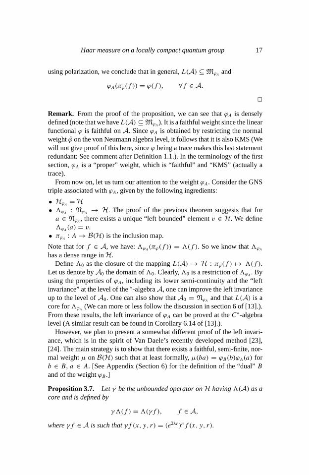
Proposition 3.7. Letγ be the unbounded operator onH having3(A) as acore and is defined by
γ3(f ) = 3(γf ), f ∈ A,
whereγf ∈ A is such thatγf (x, y, r) = (e
2λr)
n
f (x, y, r).
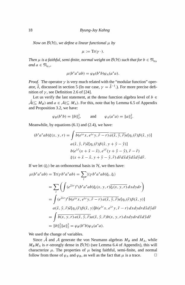
18 Byung-Jay Kahng
Now onB(H), we define a linear functionalµ by
µ := Tr(γ ·).
Thenµ is a faithful, semi-finite, normal weight onB(H) such that forb ∈ N
ϕ
B
anda ∈ N
ϕ
A
,
µ(b
∗
a
∗
ab) = ϕ
B
(b
∗
b)ϕ
A
(a
∗
a).
Proof. The operatorγ is very much related with the “modular function” oper-ator, ˜δ, discussed in section 5 (In our case,γ =
˜
δ
−1.). For more precise defi-nition of γ , see Definition 2.6 of [24].
Let us verify the last statement, at the dense function algebra level ofb ∈
ˆ
A(⊆ M
B
) anda ∈ A(⊆ M
A
). For this, note that by Lemma 6.5 of Appendixand Proposition 3.2, we have:
ϕ
B
(b
∗
b) = ‖b‖
22, and ϕ
A
(a
∗
a) = ‖a‖
22.
Meanwhile, by equations (6.1) and (2.4), we have:
(b
∗
a
∗
ab)ξ(x, y, r) =
∫
b(e
λr
x, e
λr
y, r − r) a(x, y, r)e[ηλ
(r)β(x, y)]
a(x, y, r)e[ηλ
(r)β(x, y + y − y)]
b(e
λr
(x + x − x), e
λr
(y + y − y), r − r)
ξ(x + x − x, y + y − y, r) drdxdydxdydr.
If we let (ξl
) be an orthonormal basis inH, we then have:
µ(b
∗
a
∗
ab) = Tr(γ b∗
a
∗
ab) =
∑
l
〈(γ b
∗
a
∗
ab)ξ
l
, ξ
l
〉
=
∑
l
(
∫
(e
2λr)
n
(b
∗
a
∗
ab)ξ
l
(x, y, r)ξ
l
(x, y, r) dxdydr
)
=
∫
(e
2λr)
n
b(e
λr
x, e
λr
y, r − r) a(x, y, r)e[ηλ
(r)β(x, y)]
a(x, y, r)e[ηλ
(r)β(x, y)]b(eλrx, eλry, r − r) dxdydrdxdydr
=
∫
b(x, y, r) a(x, y, r)a(x, y, r)b(x, y, r) dxdydrdxdydr
= ‖b‖
22‖a‖
22 = ϕ
B
(b
∗
b)ϕ
A
(a
∗
a).
We used the change of variables.Since ˆ
A andA generate the von Neumann algebrasMB
andMA
, whileM
B
M
A
is σ -strongly dense inB(H) (see Lemma 6.4 of Appendix), this willcharacterizeµ. The properties ofµ being faithful, semi-finite, and normalfollow from those ofϕ
A
andϕB
, as well as the fact thatµ is a trace. 2
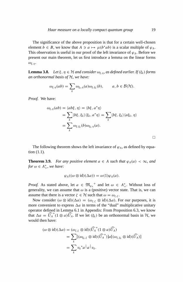
Haar measure on a locally compact quantum group 19
The significance of the above proposition is that for a certain well-chosenelementb ∈ B, we know thatA 3 a 7→ µ(b
∗
ab) is a scalar multiple ofϕA
.This observation is useful in our proof of the left invariance ofϕ
A
. Before wepresent our main theorem, let us first introduce a lemma on the linear formsω
ξ,η
.
Lemma 3.8. Letξ, η ∈ H and considerωξ,η
, as defined earlier. If(ξk
) formsan orthonormal basis ofH, we have:
ω
ξ,η
(ab) =
∑
k
ω
ξ
k
,η
(a)ω
ξ,ξ
k
(b), a, b ∈ B(H).
Proof. We have:
ω
ξ,η
(ab) = 〈abξ, η〉 = 〈bξ, a
∗
η〉
=
∑
k
〈bξ, ξ
k
〉〈ξ
k
, a
∗
η〉 =
∑
k
〈bξ, ξ
k
〉〈aξ
k
, η〉
=
∑
k
ω
ξ,ξ
k
(b)ω
ξ
k
,η
(a).
2
The following theorem shows the left invariance ofϕA
, as defined by equa-tion (1.1).
Theorem 3.9. For any positive elementa ∈ A such thatϕA
(a) < ∞, andfor ω ∈ A
∗
+
, we have:
ϕ
A
((ω ⊗ id)(1a)) = ω(1)ϕA
(a).
Proof. As stated above, leta ∈ M
ϕ
A
+ and letω ∈ A
∗
+
. Without loss ofgenerality, we can assume thatω is a (positive) vector state. That is, we canassume that there is a vectorζ ∈ H such thatω = ω
ζ,ζ
.Now consider(ω ⊗ id)(1a) = (ω
ζ,ζ
⊗ id)(1a). For our purposes, it ismore convenient to express1a in terms of the “dual” multiplicative unitaryoperator defined in Lemma 6.1 in Appendix: From Proposition 6.3, we knowthat1a =
U
A
∗
(1 ⊗ a)
U
A
. If we let (ξk
) be an orthonormal basis inH, wewould then have:
(ω ⊗ id)(1a) = (ω
ζ,ζ
⊗ id)(UA
∗
(1 ⊗ a)
U
A
)
=
∑
k
[(ωξ
k
,ζ
⊗ id)(UA
∗
)]a[(ωζ,ξ
k
⊗ id)(UA
)]
=
∑
k
v
k
∗
a
12a
12v
k
.
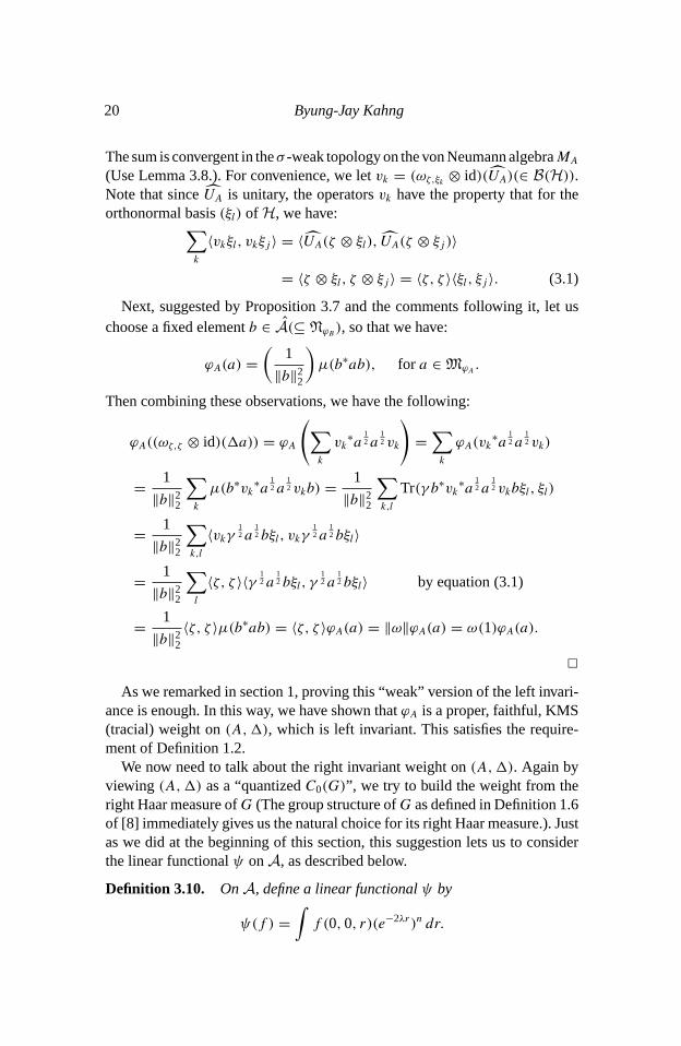
20 Byung-Jay Kahng
The sum is convergent in theσ -weak topology on the von Neumann algebraM
A
(Use Lemma 3.8.). For convenience, we letv
k
= (ω
ζ,ξ
k
⊗ id)(UA
)(∈ B(H)).Note that sinceU
A
is unitary, the operatorsvk
have the property that for theorthonormal basis(ξ
l
) of H, we have:∑
k
〈v
k
ξ
l
, v
k
ξ
j
〉 = 〈
U
A
(ζ ⊗ ξ
l
),
U
A
(ζ ⊗ ξ
j
)〉
= 〈ζ ⊗ ξ
l
, ζ ⊗ ξ
j
〉 = 〈ζ, ζ 〉〈ξ
l
, ξ
j
〉. (3.1)
Next, suggested by Proposition 3.7 and the comments following it, let uschoose a fixed elementb ∈
ˆ
A(⊆ N
ϕ
B
), so that we have:
ϕ
A
(a) =
(
1
‖b‖
22
)
µ(b
∗
ab), for a ∈ M
ϕ
A
.
Then combining these observations, we have the following:
ϕ
A
((ω
ζ,ζ
⊗ id)(1a)) = ϕ
A
(
∑
k
v
k
∗
a
12a
12v
k
)
=
∑
k
ϕ
A
(v
k
∗
a
12a
12v
k
)
=
1
‖b‖
22
∑
k
µ(b
∗
v
k
∗
a
12a
12v
k
b) =
1
‖b‖
22
∑
k,l
Tr(γ b∗
v
k
∗
a
12a
12v
k
bξ
l
, ξ
l
)
=
1
‖b‖
22
∑
k,l
〈v
k
γ
12a
12bξ
l
, v
k
γ
12a
12bξ
l
〉
=
1
‖b‖
22
∑
l
〈ζ, ζ 〉〈γ
12a
12bξ
l
, γ
12a
12bξ
l
〉 by equation (3.1)
=
1
‖b‖
22
〈ζ, ζ 〉µ(b
∗
ab) = 〈ζ, ζ 〉ϕ
A
(a) = ‖ω‖ϕ
A
(a) = ω(1)ϕA
(a).
2
As we remarked in section 1, proving this “weak” version of the left invari-ance is enough. In this way, we have shown thatϕ
A
is a proper, faithful, KMS(tracial) weight on(A,1), which is left invariant. This satisfies the require-ment of Definition 1.2.
We now need to talk about the right invariant weight on(A,1). Again byviewing (A,1) as a “quantizedC0(G)”, we try to build the weight from theright Haar measure ofG (The group structure ofG as defined in Definition 1.6of [8] immediately gives us the natural choice for its right Haar measure.). Justas we did at the beginning of this section, this suggestion lets us to considerthe linear functionalψ onA, as described below.
Definition 3.10. OnA, define a linear functionalψ by
ψ(f ) =
∫
f (0, 0, r)(e−2λr)
n
dr.
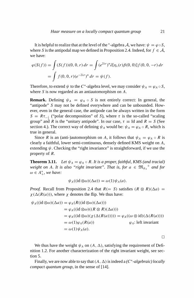
Haar measure on a locally compact quantum group 21
It is helpful to realize that at the level of the∗-algebraA, we have:ψ = ϕ◦S,whereS is the antipodal map we defined in Proposition 2.4. Indeed, forf ∈ A,we have:
ϕ(S(f )) =
∫
(S(f ))(0, 0, r) dr =
∫
(e
2λr)
n
e[ηλ
(r)β(0, 0)]f (0, 0,−r) dr
=
∫
f (0, 0, r)(e−2λr)
n
dr = ψ(f ).
Therefore, to extendψ to theC∗-algebra level, we may considerψA
= ϕ
A
◦S,whereS is now regarded as an antiautomorphism onA.
Remark. Defining ψA
= ϕ
A
◦ S is not entirely correct: In general, the“antipode” S may not be defined everywhere and can be unbounded. How-ever, even in the general case, the antipode can be always written in the formS = Rτ
−
i
2(“polar decomposition” ofS), whereτ is the so-called “scaling
group” andR is the “unitary antipode”. In our case,τ ≡ Id andR = S (Seesection 4.). The correct way of definingψ
A
would be:ψA
= ϕ
A
◦R, which istrue in general.
SinceR is an (anti-)automorphism onA, it follows thatψA
= ϕ
A
◦ R isclearly a faithful, lower semi-continuous, densely defined KMS weight onA,extendingψ . Checking the “right invariance” is straightforward, if we use theproperty ofR.
Theorem 3.11. LetψA
= ϕ
A
◦ R. It is a proper, faithful, KMS (and tracial)weight onA. It is also “right invariant”. That is, for a ∈ M
ψ
A
+ and forω ∈ A
∗
+
, we have:
ψ
A
((id ⊗ω)(1a)) = ω(1)ψA
(a).
Proof. Recall from Proposition 2.4 thatR(= S) satisfies(R ⊗ R)(1a) =
χ(1(R(a))), whereχ denotes the flip. We thus have:
ψ
A
((id ⊗ω)(1a)) = ϕ
A
(R((id ⊗ω)(1a)))
= ϕ
A
((id ⊗ω)((R ⊗ R)(1a)))
= ϕ
A
((id ⊗ω)(χ(1(R(a))))) = ϕ
A
((ω ⊗ id)(1(R(a))))
= ω(1)ϕA
(R(a)) ϕ
A
: left invariant
= ω(1)ψA
(a).
2
We thus have the weightψA
on (A,1), satisfying the requirement of Defi-nition 1.2. For another characterization of the right invariant weight, see sec-tion 5.
Finally, we are now able to say that(A,1) is indeed a(C∗-algebraic) locallycompact quantum group, in the sense of [14].

22 Byung-Jay Kahng
Theorem 3.12. The pair(A,1), together with the weightsϕA
andψA
on it,is aC∗-algebraic locally compact quantum group.
Proof. Combine the results of Proposition 2.1 and Proposition 2.3 on thecomultiplication1. Theorem 3.6 and Theorem 3.9 gives the left invariantweightφ
A
, while Theorem 3.11 gives the right invariant weightψ
A
. By Defini-tion 1.2, we conclude that(A,1) is a(reduced)C∗-algebraic quantum group.
2
4. Antipode
According to the general theory (by Kustermans and Vaes [14]), the result ofTheorem 3.12 is enough to establish our main goal of showing that(A,1) isindeed aC∗-algebraic locally compact quantum group (satisfying Definition1.2).
Assuming both the left invariant and the right invariant weights in the defi-nition may look somewhat peculiar, while there is no mention on the antipode.However, using these rather simple set of axioms, Kustermans and Vaes couldprove additional properties for(A,1), so that it can be legitimately called alocally compact quantum group. They first construct a manageable multiplica-tive unitary operator (in the sense of [2] and [27]) associated with(A,1). [Inour case, this unitary operatorW coincides with ourU
A
defined in Appendix.]More significantly, they then construct the antipode and its polar decomposi-tion. The uniqueness (up to scalar multiplication) of the Haar weight is alsoobtained.
An aspect of note through all this is that in this new definition, the “left(or right) invariance” of a weight has been formulated without invoking theantipode, while a characterization of the antipode is given without explicitlyreferring to any invariant weights. This is much simpler and is a fundamen-tal improvement over earlier frameworks, where one usually requires certainconditions of the type:
(id ⊗ϕ)((1 ⊗ a)(1b)) = S((id ⊗ϕ)((1a)(1 ⊗ b))).
It is also more natural. Note that in the cases of ordinary locally compact groupsor Hopf algebras in the purely algebraic setting, the axioms of the antipode donot have to require any relationships to invariant measures.
For details on the general theory, we will refer the reader to [14]. Whatwe plan to do in this section is to match the general theory with our specificexample. Let us see if we can re-constructS from (A,1).
By general theory ([27], [14]), the antipode,S, can be characterized suchthat{(ω ⊗ id)(U
A
) : ω ∈ B(H)
∗
} is a core forS and
S((ω ⊗ id)(UA
)) = (ω ⊗ id)(UA
∗
), ω ∈ B(H)
∗
. (4.1)

Haar measure on a locally compact quantum group 23
It is a closed linear operator onA. The domainD(S) is a subalgebra ofAandS is antimultiplicative: i. e.S(ab) = S(b)S(a), for anya, b ∈ D(S). TheimageS(D(S)) coincides withD(S)∗ andS(S(a)∗)∗ = a for anya ∈ D(S).The operatorS admits the (unique) “polar decomposition”:S = Rτ
−
i
2, where
R is the “unitary antipode” andτ−
i
2is the analytic generator of a certain one
parameter group(τt
)
t∈R
of ∗-automorphisms ofA (called the “scaling group”).
Remark. In [14], the scaling group and the unitary antipode are constructedfirst (using only the multiplicative unitary operator and the invariant weights),from which they define the antipode viaS = Rτ
−
i
2. The characterization given
above is due to Woronowicz [27].To compareS given by equation (4.1) with our ownS defined in Proposi-
tion 2.4, let us again considerωξ,η
. From the proof of Proposition 2.2, we knowthat
(ω
ξ,η
⊗ id)(UA
) = L
f
,
where
f (x, y, r) =
∫
ξ(x, y, r + r)(e
λr
)
n
η(e
λr
x, e
λr
y, r) dr.
We can carry out a similar computation for(ωξ,η
⊗ id)(UA
∗
). For ζ ∈ H,we would have (again using change of variables):
(S(L
f
))ζ(x, y, r) = S((ω
ξ,η
⊗ id)(UA
))ζ(x, y, r)
= (ω
ξ,η
⊗ id)(UA
∗
)ζ(x, y, r)
=
∫
(U
A
∗
(ξ ⊗ ζ ))(x, y, r; x, y, r)η(x, y, r) dxdydr
=
∫
g(x, y, r)ζ(x−x, y−y, r)e[ηλ
(r)β(x, y−y)] dxdy
= L
g
ζ(x, y, r),
where
g(x, y, r) =
∫
(e
λr
)
n
ξ(−e
λr
x,−e
λr
y, r − r)η(−x,−y, r)
e[ηλ
(r)β(x, y)] dr.
This means thatS(f ) = g. Comparing withf , we see that
(S(f ))(x, y, r) = g(x, y, r) = (e
2λr)
n
f (−e
λr
x,−e
λr
y,−r)e[ηλ
(r)β(x, y)].
This is exactly the expression we gave in Proposition 2.4, verifying that oursituation agrees perfectly with the general theory.

24 Byung-Jay Kahng
Since we have already seen thatS : A → A is an antiautomorphism (definedeverywhere onA), the uniqueness of the polar decomposition implies thatR = S andτ ≡ Id.
As a final comment on the general theory, we point out that after one definesthe antipode asS = Rτ
−
12, one proves that fora, b ∈ N
ψ
A
,
S((ψ
A
⊗ id)((a∗
⊗ 1)(1b))) = (ψ
A
⊗ id)(1(a∗
)(b ⊗ 1)).
In this way, one can “define”S, as well as give a stronger version of theinvariance ofψ
A
. The fact that this result could be obtained from the definingaxioms (as opposed to being one of the axioms itself) was the significantachievement of [14].
5. Modular function
To motivate the modular function of(A,1), let us re-visit our right invariantweightψ
A
. We will keep the notation of Section 3. Recall that at the level of thedense∗-algebraA, the right invariant weight is given by the linear functionalψ :
ψ(f ) =
∫
f (0, 0, r)(e−2λr)
n
dr.
Let us consider the Hilbert spaceHR
, which will be the GNS Hilbert spacefor ψ . It is defined such thatH
R
= H as a space and the inner product on it isdefined by
〈f, g〉
R
=
∫
f (x, y, r)g(x, y, r)(e
−2λr)
n
dr.
Let 3R
be the inclusion map3R
: A ↪→ H
R
. We can see easily that forf, g ∈ A,
〈3
R
(f ),3
R
(g)〉
R
= 〈3(f ),3(δg)〉.
Hereδg ∈ A defined byδg(x, y, r) = (e
−2λr)
n
g(x, y, r).For motivational purposes, let us be less rigorous for the time being. Observe
that working purely formally, we can regardδg as follows:
δg(x, y, r) = (e
−2λr)
n
g(x, y, r)
=
∫
δ(x, y, r)g(x − x, y − y, r)e[ηλ
(r)β(x, y − y)] dxdy
= (δ × g)(x, y, r),
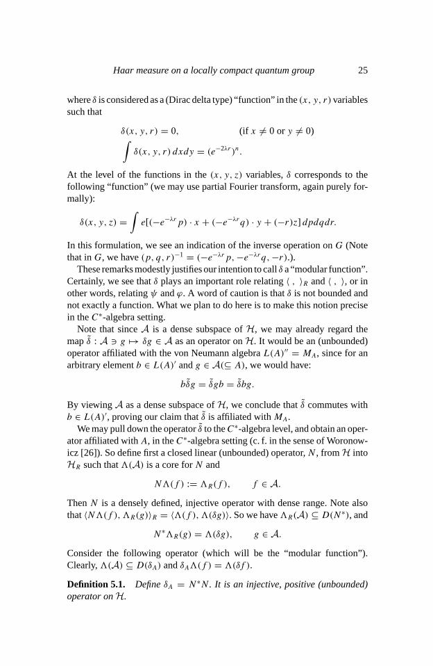
Haar measure on a locally compact quantum group 25
whereδ is considered as a (Dirac delta type) “function” in the(x, y, r) variablessuch that
δ(x, y, r) = 0, (if x 6= 0 ory 6= 0)∫
δ(x, y, r) dxdy = (e
−2λr)
n
.
At the level of the functions in the(x, y, z) variables,δ corresponds to thefollowing “function” (we may use partial Fourier transform, again purely for-mally):
δ(x, y, z) =
∫
e[(−e−λrp) · x + (−e
−λr
q) · y + (−r)z] dpdqdr.
In this formulation, we see an indication of the inverse operation onG (Notethat inG, we have(p, q, r)−1
= (−e
−λr
p,−e
−λr
q,−r).).These remarks modestly justifies our intention to callδ a “modular function”.
Certainly, we see thatδ plays an important role relating〈 , 〉
R
and〈 , 〉, or inother words, relatingψ andϕ. A word of caution is thatδ is not bounded andnot exactly a function. What we plan to do here is to make this notion precisein theC∗-algebra setting.
Note that sinceA is a dense subspace ofH, we may already regard themap ˜
δ : A 3 g 7→ δg ∈ A as an operator onH. It would be an (unbounded)operator affiliated with the von Neumann algebraL(A)′′ = M
A
, since for anarbitrary elementb ∈ L(A)
′ andg ∈ A(⊆ A), we would have:
b
˜
δg =
˜
δgb =
˜
δbg.
By viewing A as a dense subspace ofH, we conclude that˜δ commutes withb ∈ L(A)
′, proving our claim that˜δ is affiliated withMA
.We may pull down the operator˜δ to theC∗-algebra level, and obtain an oper-
ator affiliated withA, in theC∗-algebra setting (c. f. in the sense of Woronow-icz [26]). So define first a closed linear (unbounded) operator,N , fromH intoH
R
such that3(A) is a core forN and
N3(f ) := 3
R
(f ), f ∈ A.
ThenN is a densely defined, injective operator with dense range. Note alsothat〈N3(f ),3
R
(g)〉
R
= 〈3(f ),3(δg)〉. So we have3R
(A) ⊆ D(N
∗
), and
N
∗
3
R
(g) = 3(δg), g ∈ A.
Consider the following operator (which will be the “modular function”).Clearly,3(A) ⊆ D(δ
A
) andδA
3(f ) = 3(δf ).
Definition 5.1. DefineδA
= N
∗
N . It is an injective, positive (unbounded)operator onH.

26 Byung-Jay Kahng
By general theory, we can say thatδA
is the appropriate definition of the“modular function” in theC∗-algebra setting.
Theorem 5.2. LetδA
be defined as above. Then the following properties hold.
(1) δA
is an operator affiliated with theC∗-algebraA.(2) 1(δ
A
) = δ
A
⊗ δ
A
.(3) τ
t
(δ
A
) = δ
A
andR(δA
) = δ
−1A
.
(4) ψ(a) = ϕ(δ
12A
aδ
12A
), for a ∈ A.
Proof. It is not difficult to see thatδA
is cut down from the operator˜δ. Forproof of the statements, see [14, §7] or see [13, §8]. There are also importantrelations relating the modular automorphism groups corresponding toϕ
A
andψ
A
, but in our case they become trivial. 2
6. Appendix: An alternative formulation of the dual
The aim of this Appendix is to present a dual counterpart to our locally compactquantum group(A,1), which is slightly different (though isomorphic) from(
ˆ
A,
ˆ
1) defined in Section 2. It would be actually the HopfC∗-algebra havingthe opposite multiplication and the opposite comultiplication to( ˆ
A,
ˆ
1). Toavoid a lengthy discussion, we plan to give only a brief treatment. But we willinclude results that are relevant to our main theorem in Section 3.
Let us define(B,1B
), by again using the language of multiplicative unitaryoperators. We begin with a lemma, which is motivated by the general theoryof multiplicative unitary operators [2].
Lemma 6.1. Let j ∈ B(H) be defined by
jξ(x, y, r) = (e
λr
)
n
e[ηλ
(r)β(x, y)]ξ(−eλrx,−eλry,−r).
Thenj is a unitary operator such thatj2= 1. Moreover, the operatorU
A
defined by
U
A
= 6(j ⊗ 1)UA
(j ⊗ 1)6, 6 denotes the flip
is multiplicative unitary and is regular. Forξ ∈ H, we specifically have:
U
A
ξ(x, y, r, x
′
, y
′
, r
′
) = e[ηλ
(r)β(e
λ(r
′
−r)
x
′
, y)]
ξ(x + e
λ(r
′
−r)
x
′
, y + e
λ(r
′
−r)
y
′
, r; x
′
, y
′
, r
′
− r).
Remark. The proof is straightforward. What is really going on is that the triple(H, U
A
, j) forms aKac system, in the terminology of Baaj and Skandalis (Seesection 6 of [2].). The operatorj may be written asj =
ˆ
JJ = J
ˆ
J , where ˆ
J

Haar measure on a locally compact quantum group 27
is the anti-unitary operator defined in the proof of Proposition 2.4, whileJ isthe anti-unitary operator determining the∗-operation ofA as mentioned in theremark following Proposition 3.5. We will have an occasion to say more aboutthese operators in our future paper.
Definition 6.2. LetUA
be the multiplicative unitary operator obtained above.Define(B,1
B
) as follows:
(1) LetA(UA
) be the subspace ofB(H) defined by
A(
U
A
) = {(ω ⊗ id)( ˆ
U
A
) : ω ∈ B(H)
∗
}.
ThenA(
U
A
) is a subalgebra ofB(H), and the subspaceA(UA
)H formsa total set inH.
(2) The norm-closure inB(H) of the algebraA(UA
) is theC∗-algebraB. Theσ -strong closure ofA(U
A
) in B(H)will be the von Neumann algebraMB
.(3) For b ∈ A(
U
A
), define1B
(b) by1B
(b) =
U
A
(b⊗ 1)UA
∗
. Then1B
canbe extended to the comultiplication onB, and also to the level of the vonNeumann algebraM
B
.
We do not give the proof here, since it is essentially the same as in Propo-sitions 2.2 and 2.6. Let us just add a brief clarification: By a comultiplicationonB, we mean a non-degenerateC∗-homomorphism1
B
: B → M(B ⊗ B)
satisfying the coassociativity; whereas by a comultiplication onM
B
, we meana unital normal∗-homomorphism1
B
: MB
→ M
B
⊗M
B
satisfying the coas-sociativity. In the following proposition, we give a more specific descriptionof theC∗-algebraB.
Proposition 6.3. (1) Forω ∈ B(H)
∗
, we letλ(ω) = (ω⊗ id)(UA
). Then wehave:λ(ω) = jρ(ω)j , whereρ(ω) = (id ⊗ω)(U
A
) ∈
ˆ
A(U
A
) as definedin equation(2.5).
(2) Let ˆ
A be the space of Schwartz functions in the(x, y, r) variables havingcompact support in ther variable. Forf ∈
ˆ
A, define the operatorλf
∈
B(H) by
(λ
f
ζ )(x, y, r) =
∫
f (e
λr
x, e
λr
y, r − r)ζ(x, y, r) dr. (6.1)
Then theC∗-algebraB is generated by the operatorsλf
. By partialFourier transform, we can also show thatB ∼
=
λ(C
∗
(G)), whereλ is theleft regular representation ofC∗
(G).(3) For anyf, g ∈
ˆ
A, we have:[ρf
, λ
g
] = 0. Actually,MB
= M
ˆ
A
′, whereM
ˆ
A
is the von Neumann algebra generated byˆ
A.(4) For b ∈ (
ˆ
A,
ˆ
1), we have:(λ⊗ λ)(
ˆ
1b) =
U
A
(λ(b)⊗ 1)UA
∗
.
28 Byung-Jay Kahng
(5) Dually, there exists an alternative characterization of theC∗-algebraA:
A = {(id ⊗ω)(
U
A
) : ω ∈ B(H)
∗
}
‖ ‖
.
And fora ∈ A, we have:(L⊗ L)(1a) =
U
A
∗
(1 ⊗ L(a))
U
A
, whereL isthe regular representation ofA defined in Section 2.
Proof. See Proposition 6.8 of [2]. For instance, for the first statement, notethat:
λ(ω) = (id ⊗ω)((j ⊗ 1)UA
(j ⊗ 1)) = jρ(ω)j.
The second statement is a consequence of this result. We can also give a directproof, just as in Propositions 2.2 and 2.6. Actually, we have:
jρ
f
j = λ
˜
f
, f ∈
ˆ
A,
where ˜
f (x, y, r) = e[ηλ
(r)β(x, y)]f (−eλrx,−eλry,−r).For the third and fourth statements, we can again refer to general theory
(Proposition 6.8 of [2]), or we can just give a direct proof. Since we see (up topartial Fourier transform in thex andy variables) thatρ
f
andλf
are essentiallythe right and left regular representations ofC
∗
(G), the result follows easily.The last statement is also straightforward (similar to Proposition 2.2).2
Remark. The above proposition implies that at least at the level of the densesubalgebra of functions,B has an opposite algebra structure to that ofˆ
A.Meanwhile, (4) above implies that( ˆ
A,
ˆ
1)
∼
=
(B,1
B
) as HopfC∗-algebras.It turns out that working with(B,1
B
) andMB
= M
ˆ
A
′ is more convenientin our proof of Theorem 3.9. Here are a couple of lemmas that are useful inSection 3. Similar results exist forˆA andM
ˆ
A
. We took light versions of theproofs.
Lemma 6.4. LetMA
andMB
be the enveloping von Neumann algebras ofA
andB. We have:
(1) UA
∈ M
A
⊗M
B
.(2) M
B
∩M
A
= C1.(3) The linear spaceM
B
M
A
is σ -strongly dense inB(H).
Proof. The first statement is immediate from general theory, once we realize(see previous proposition) thatU
A
determinesB andA (as well asMB
andMA
).We also have:U
A
∈ M(A⊗B). The remaining two results also follow from thesame realization. For instance, we could modify the proof of Proposition 2.5of [24]. 2

Haar measure on a locally compact quantum group 29
Lemma 6.5. On ˆ
A ⊆ B, consider a linear functionalϕB
defined by
ϕ
B
(λ
f
) =
∫
f (x, y,0) dxdy.
It can be extended to a faithful, semi-finite, normal weightϕ
B
onMB
.
Remark. The idea for proof of this lemma is pretty much the same as theearly part of section 3 (butϕ
B
is no longer a trace). It turns out thatϕB
will bean (invariant) Haar weight for(B,1
B
), although for our current purposes, thisresult is not immediately necessary. We will make all these clear in our futurepaper. Meanwhile, by a straightforward calculation using equation (6.1), wesee easily that:
ϕ
B
(λ
f
∗
λ
f
) = ‖f ‖
22.
This last result will be useful in the proof of Proposition 3.7.Using multiplicative unitary operators, we can also give notions that are
analogous to “opposite dual” or “co-opposite dual” [11]. For a more carefuldiscussion on the duality, as well as on the notion of quantum double, refer toour future paper.
References
[1] S. Baaj,Representation r´eguliere du groupe quantique des d´eplacements de Woronow-icz, Recent Advances in Operator Algebras (Orleans 1992), Asterisque, no. 232, Soc.Math. France, 1995, pp. 11–48 (French).
[2] S. Baaj and G. Skandalis,Unitaires multiplicatifs et dualit´e pour les produits crois´esdeC∗-algebres, Ann. Scient.Ec. Norm. Sup., 4e seriet. 26 (1993), 425–488 (French).
[3] F. Combes,Poids sur uneC∗-algebre, J. Math. Pures et Appl.47 (1968), 57–100(French).
[4] —————, Poids associ´e a une algebre hilbertienne `a gauche, Compos. Math.23(1971), 49–77 (French).
[5] A. Connes,Noncommutative Geometry, Academic Press, 1994.[6] M. Enock and J. M. Schwartz,Kac Algebras and Duality of Locally Compact Groups,
Springer-Verlag, 1992.[7] M. Enock and L. Vainerman,Deformation of a Kac algebra by an abelian subgroup,
Comm. Math. Phys.178(1996), 571–595.[8] B. J. Kahng,Non-compact quantum groups arising from Heisenberg type Lie bialge-
bras, J. Operator Theory44 (2000), 303–334.[9] —————, ∗-representations of a quantum Heisenberg group algebra, Houston J.
Math.28 (2002), 529–552.[10] —————, Dressing orbits and a quantum Heisenberg group algebra, 2002, preprint
(available as math.OA/0211003, at http://lanl.arXiv.org).[11] —————, Construction of a quantum Heisenberg group, 2003, preprint (available
as math.OA/0307126, at http://lanl.arXiv.org).[12] J. Kustermans,KMS-weights onC∗-algebras, 1997, preprint, Odense Universitet
(available as funct-an/9704008, at http://lanl.arXiv.org).

30 Byung-Jay Kahng
[13] J. Kustermans and A. Van Daele,C∗-algebraic quantum groups arising from algebraicquantum groups, Int. J. Math.8 (1997), no. 8, 1067–1139.
[14] J. Kustermans and S. Vaes,Locally compact quantum groups, Ann. Scient.Ec. Norm.Sup., 4e serie t. 33 (2000), 837–934.
[15] T. Masuda and Y. Nakagami,A von Neumann algebra framework for the duality ofthe quantum groups, Publ. RIMS, Kyoto Univ.30 (1994), no. 5, 799–850.
[16] S. Montgomery,Hopf Algebras and Their Actions on Rings, CBMS Regional Confer-ence Series in Mathematics, no. 82, American Mathematical Society, 1993.
[17] J. Packer and I. Raeburn,Twisted crossed products ofC∗-algebras, Math. Proc. Cam-bridge Philos. Soc.106(1989), 293–311.
[18] M. A. Rieffel,Deformation quantization of Heisenberg manifolds, Comm. Math. Phys.122(1989), 531–562.
[19] —————, Some solvable quantum groups, Operator Algebras and Topology (W. B.Arveson, A. S. Mischenko, M. Putinar, M. A. Rieffel, and S. Stratila, eds.), Proc.OATE2 Conf: Romania 1989, Pitman Research Notes Math., no. 270, Longman, 1992,pp. 146–159.
[20] —————, Deformation quantization for actions ofRd , Memoirs of the AMS, no.506, American Mathematical Society, Providence, RI, 1993.
[21] S. Stratila,Modular Theory in Operator Algebras, Abacus Press, 1981.[22] S. Vaes and L. Vainerman,Extensions of locally compact quantum groups and the
bicrossed product construction, Adv. Math.175(2003), 1–101.[23] A. Van Daele,The Haar measure on some locally compact quantum groups, 2001,
preprint (available as math.OA/0109004, at http://lanl.arXiv.org).[24] —————, The Heisenberg commutation relations, commuting squares and the Haar
measure on locally compact quantum groups, 2001, preprint (to appear in Proceedingsof the OAMP Conference, Constantza, 2001).
[25] S. L. Woronowicz,TwistedSU(2) group. an example of noncommutative differentialcalculus, Publ. RIMS, Kyoto Univ.23 (1987), 117–181.
[26] —————, Unbounded elements affiliated withC∗-algebras and non-compact quan-tum groups, Comm. Math. Phys.136(1991), 399–432.
[27] —————, From multiplicative unitaries to quantum groups, Int. J. Math.7 (1996),no. 1, 127–149.