HYPERNETWORKS

David Ha∗, Andrew Dai, Quoc V. LeGoogle Brain{hadavid,adai,qvl}@google.com

ABSTRACT

This work explores hypernetworks: an approach of using a one network, alsoknown as a hypernetwork, to generate the weights for another network. Hypernet-works provide an abstraction that is similar to what is found in nature: the relation-ship between a genotype – the hypernetwork – and a phenotype – the main net-work. Though they are also reminiscent of HyperNEAT in evolution, our hyper-networks are trained end-to-end with backpropagation and thus are usually faster.The focus of this work is to make hypernetworks useful for deep convolutionalnetworks and long recurrent networks, where hypernetworks can be viewed as re-laxed form of weight-sharing across layers. Our main result is that hypernetworkscan generate non-shared weights for LSTM and achieve near state-of-the-art re-sults on a variety of sequence modelling tasks including character-level languagemodelling, handwriting generation and neural machine translation, challengingthe weight-sharing paradigm for recurrent networks. Our results also show thathypernetworks applied to convolutional networks still achieve respectable resultsfor image recognition tasks compared to state-of-the-art baseline models whilerequiring fewer learnable parameters.

1 INTRODUCTION

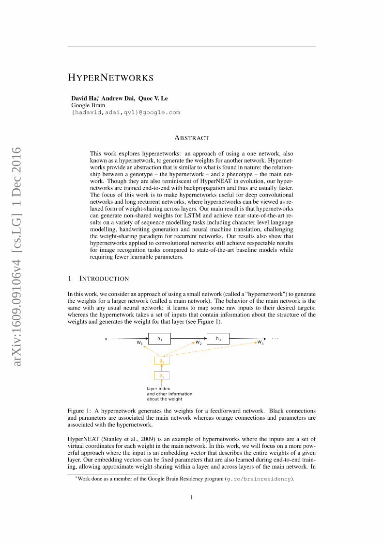
In this work, we consider an approach of using a small network (called a “hypernetwork") to generatethe weights for a larger network (called a main network). The behavior of the main network is thesame with any usual neural network: it learns to map some raw inputs to their desired targets;whereas the hypernetwork takes a set of inputs that contain information about the structure of theweights and generates the weight for that layer (see Figure 1).

Figure 1: A hypernetwork generates the weights for a feedforward network. Black connectionsand parameters are associated the main network whereas orange connections and parameters areassociated with the hypernetwork.

HyperNEAT (Stanley et al., 2009) is an example of hypernetworks where the inputs are a set ofvirtual coordinates for each weight in the main network. In this work, we will focus on a more pow-erful approach where the input is an embedding vector that describes the entire weights of a givenlayer. Our embedding vectors can be fixed parameters that are also learned during end-to-end train-ing, allowing approximate weight-sharing within a layer and across layers of the main network. In

∗Work done as a member of the Google Brain Residency program (g.co/brainresidency).

1

arX

iv:1

609.

0910

6v4

[cs

.LG

] 1

Dec

201

6

addition, our embedding vectors can also be generated dynamically by our hypernetwork, allowingthe weights of a recurrent network to change over timesteps and also adapt to the input sequence.

We perform experiments to investigate the behaviors of hypernetworks in a range of contexts andfind that hypernetworks mix well with other techniques such as batch normalization and layer nor-malization. Our main result is that hypernetworks can generate non-shared weights for LSTM thatwork better than the standard version of LSTM (Hochreiter & Schmidhuber, 1997). On languagemodelling tasks with Character Penn Treebank, Hutter Prize Wikipedia datasets, hypernetworks forLSTM achieve near state-of-the-art results. On a handwriting generation task with IAM handwrit-ing dataset, Hypernetworks for LSTM achieves high quantitative and qualitative results. On imageclassification with CIFAR-10, hypernetworks, when being used to generate weights for a deep con-vnet (LeCun et al., 1990), obtain respectable results compared to state-of-the-art models while hav-ing fewer learnable parameters. In addition to simple tasks, we show that Hypernetworks for LSTMoffers an increase in performance for large, production-level neural machine translation models.

2 MOTIVATION AND RELATED WORK

Our approach is inspired by methods in evolutionary computing, where it is difficult to directlyoperate in large search spaces consisting of millions of weight parameters. A more efficient methodis to evolve a smaller network to generate the structure of weights for a larger network, so that thesearch is constrained within the much smaller weight space. An instance of this approach is the workon the HyperNEAT framework (Stanley et al., 2009). In the HyperNEAT framework, CompositionalPattern-Producing Networks (CPPNs) are evolved to define the weight structure of much largermain network. Closely related to our approach is a simplified variation of HyperNEAT, where thestructure is fixed and the weights are evolved through Discrete Cosine Transform (DCT) is calledCompressed Weight Search (Koutnik et al., 2010). Even more closely related to our approach areDifferentiable Pattern Producing Networks (DPPNs), where the structure is evolved but the weightsare learned (Fernando et al., 2016), and ACDC-Networks (Moczulski et al., 2015), where linearlayers are compressed with DCT and the parameters are learned.

Most reported results using these methods, however, are in small scales, perhaps because they areboth slow to train and require heuristics to be efficient. The main difference between our approachand HyperNEAT is that hypernetworks in our approach are trained end-to-end with gradient descenttogether with the main network, and therefore are more efficient.

In addition to end-to-end learning with gradient descent, our approach strikes a good balance be-tween Compressed Weight Search and HyperNEAT in terms of model flexibility and training sim-plicity. First, it can be argued that Discrete Cosine Transform used in Compressed Weight Searchmay be too simple and using the DCT prior may not be suitable for many problems. Second, eventhough HyperNEAT is more flexible, evolving both the architecture and the weights in HyperNEATis often an overkill for most practical problems.

Even before the work on HyperNEAT and DCT, Schmidhuber (1992; 1993) has suggested the con-cept of fast weights in which one network can produce context-dependent weight changes for asecond network. Small scale experiments were conducted to demonstrate fast weights for feed for-ward networks at the time, but perhaps due to the lack of modern computational tools, the recurrentnetwork version was mentioned mainly as a thought experiment (Schmidhuber, 1993). A subse-quent work demonstrated practical applications of fast weights (Gomez & Schmidhuber, 2005),where a generator network is learnt through evolution to solve an artificial control problem. Theconcept of a network interacting with another network is central to the work of (Jaderberg et al.,2016; Andrychowicz et al., 2016), and especially (Denil et al., 2013; Yang et al., 2015; Bertinettoet al., 2016; De Brabandere et al., 2016), where certain parameters in a convolutional network arepredicted by another network. These studies however did not explore the use of this approach torecurrent networks, which is a main contribution of our work.

The focus of this work is to generate weights for practical architectures, such as convolutional net-works and recurrent networks by taking layer embedding vectors as inputs. However, our hypernet-works can also be utilized to generate weights for a fully connected network by taking coordinateinformation as inputs similar to DPPNs. Using this setting, hypernetworks can approximately re-

2

cover the convolutional architecture without explicitly being told to do so, a similar result obtainedby “Convolution by Evolution" (Fernando et al., 2016). This result is described in Appendix A.1.

3 METHODS

In this paper, we view convolutional networks and recurrent networks as two ends of a spectrum.On one end, recurrent networks can be seen as imposing weight-sharing across layers, which makesthem inflexible and difficult to learn due to vanishing gradient. On the other end, convolutionalnetworks enjoy the flexibility of not having weight-sharing, at the expense of having redundantparameters when the networks are deep. Hypernetworks can be seen as a form of relaxed weight-sharing, and therefore strikes a balance between the two ends. See Appendix A.2 for conceptualdiagrams of Static and Dynamic Hypernetworks.

3.1 STATIC HYPERNETWORK: A WEIGHT FACTORIZATION APPROACH FOR DEEPCONVOLUTIONAL NETWORKS

First we will describe how we construct a hypernetwork for the purpose of generating the weightsof a feedforward convolutional network. In a typical deep convolutional network, the majority ofmodel parameters are in the kernels of convolutional layers. Each kernel contain Nin ×Nout filtersand each filter has dimensions fsize × fsize. Let’s suppose that these parameters are stored in amatrix Kj ∈ RNinfsize×Noutfsize for each layer j = 1, .., D, where D is the depth of the mainconvolutional network. For each layer j, the hypernetwork receives a layer embedding zj ∈ RNz asinput and predicts Kj , which can be generally written as follows:

Kj = g(zj), ∀j = 1, ..., D (1)

We note that this matrix Kj can be broken down as Nin slices of a smaller matrix with dimensionsfsize×Noutfsize, each slice of the kernel is denoted asKj

i ∈ Rfsize×Noutfsize . Therefore, in our ap-proach, the hypernetwork is a two-layer linear network. The first layer of the hypernetwork takes theinput vector zj and linearly projects it into theNin inputs, withNin different matricesWi ∈ Rd×Nz

and bias vectors Bi ∈ Rd, where d is the size of the hidden layer in the hypernetwork. For our pur-pose, we fix d to be equal to Nz although they can be different. The final layer of the hypernetworkis a linear operation which takes an input vector ai of size d and linearly projects that into Ki usinga common tensor Wout ∈ Rfsize×Noutfsize×d and bias matrix Bout ∈ Rfsize×Noutfsize . The finalkernel Kj will be a concatenation of every Kj

i . Thus g(zj) can be written as follows:

aji =Wizj +Bi, ∀i = 1, .., Nin,∀j = 1, ..., D

Kji = 〈Wout, a

ji 〉 1 +Bout, ∀i = 1, .., Nin,∀j = 1, ..., D

Kj =(Kj

1 Kj2 ... Kj

i ... KjNin

), ∀j = 1, ..., D

(2)

In our formulation, the learnable parameters are Wi, Bi, Wout, Bout together with all zj’s. Duringinference, the model simply takes the layer embeddings zj learned during training to reproducethe kernel weights for layer j in the main convolutional network. As a side effect, the number oflearnable parameters in hypernetwork will be much lower than the main convolutional network. Infact, the total number of learnable parameters in hypernetwork is Nz ×D + d× (Nz + 1)×Ni +fsize×Nout× fsize× (d+1) compared to the D×Nin× fsize×Nout× fsize parameters for thekernels of the main convolutional network.

Our approach of constructing g(.) is similar to the hierarchically semiseparable matrix approachproposed by Xia et al. (2010). Note that even though it seems redundant to have a two-layered linearhypernetwork as that is equivalent to a one-layered hypernetwork, the fact that Wout and Bout areshared makes our two-layered hypernetwork more compact than a one-layered hypernetwork. Moreconcretely, a one-layered hypernetwork would have Nz × Nin × fsize × Nout × fsize learnableparameters which is usually much bigger than a two-layered hypernetwork does.

1Tensor dot product between W ∈ Rm×n×d and a ∈ Rd. Result 〈W,a〉 ∈ Rm×n

3

The above formulation assumes that the network architecture consists of kernels with same dimen-sions. In practice, deep convolutional network architectures consists of kernels of varying dimen-sions. Typically, in many designs, the kernel dimensions are integer multiples of a basic size. Thisis indeed the case in the residual network family of architectures (He et al., 2016a) that we will beexperimenting with later is an example of such a design. In our experiments, although the kernels ofa residual network do not share the same dimensions, the Ni and Nout dimensions for each kernelare integer multiples of 16. To modify our approach to work with this architecture, we have ourhypernetwork generate kernels for this basic size of 16, and if we require a larger kernel for a certainlayer, we will concatenate multiple basic kernels together to form the larger kernel.

K32×64 =

(K1 K2 K3 K4

K5 K6 K7 K8

)(3)

For example, if we need to generate a kernel with Ni = 32 and Nout = 64, we will tile eight basickernels together. Each basic kernel is generated by a unique z embedding, hence the larger kernelwill be expressed with eight embeddings. Therefore, kernels that are larger in size will requirea proportionally larger number of embedding vectors. For visualizations of concatenated kernels,please see Appendix A.2.1. Figure 2 shows the similarity between kernels learned by a ConvNet toclassify MNIST digits and those learned by a hypernetwork generating weights for a ConvNet.

Figure 2: Kernels learned by a ConvNet to classify MNIST digits (left). Kernels learned by ahypernetwork generating weights for the ConvNet (right).

3.2 DYNAMIC HYPERNETWORK: ADAPTIVE WEIGHT GENERATION FOR RECURRENTNETWORKS

In the previous section, we outlined a procedure for using a hypernetwork to generate the weights fora deep convolutional network. In this section, we will use a recurrent network to dynamically gener-ate weights for another recurrent network, such that the weights can vary across many timesteps. Inthis context, hypernetworks are called dynamic hypernetworks, and can be seen as a form of relaxedweight-sharing, a compromise between hard weight-sharing of traditional recurrent networks, andno weight-sharing of convolutional networks. This relaxed weight-sharing approach allows us tocontrol the trade off between the number of model parameters and model expressiveness.

Our dynamic hypernetworks can be used to generate weights for RNN and LSTM. When a hyper-network is used to generate the weights for an RNN, it is called HyperRNN. At every time step t,a HyperRNN takes as input the concatenated vector of input xt and the hidden states of the mainRNN ht−1, it then generates as output the vector ht. This vector is then used to generate the weightsfor the main RNN at the same timestep. Both the HyperRNN and the main RNN are trained jointlywith backpropagation and gradient descent. In the following, we will give a more formal descriptionof the model.

The standard formulation of a Basic RNN is given by:ht = φ(Whht−1 +Wxxt + b) (4)

4

where ht is the hidden state, φ is a non-linear operation such as tanh or relu, and the weightmatrices and bias Wh ∈ RNh×Nh ,Wx ∈ RNh×Nx , b ∈ RNh is fixed each timestep for an inputsequence X = (x1, x2, . . . , xT ).

Figure 3: An overview of HyperRNNs. Black connections and parameters are associated basicRNNs. Orange connections and parameters are introduced in this work and associated with Hyper-RNNs. Dotted arrows are for parameter generation.

In HyperRNN, we allow Wh and Wx to float over time by using a smaller hypernetwork to generatethese parameters of the main RNN at each step (see Figure 3). More concretely, the parametersWh,Wx, b of the main RNN are different at different time steps, so that ht can now be computed as:

ht = φ(Wh(zh)ht−1 +Wx(zx) + b(zb)

), where

Wh(zh) = 〈Whz, zh〉Wx(zx) = 〈Wxz, zx〉b(zb) =Wbzzb + b0

(5)

Where Whz ∈ RNh×Nh×Nz ,Wxz ∈ RNh×Nx×Nz ,Wbz ∈ RNh×Nz , b0 ∈ RNh and zh, zx, zz ∈RNz . We use a recurrent hypernetwork to compute zh, zx and zb as a function of xt and ht−1:

xt =

(ht−1

xt

)

ht = φ(Whht−1 +Wxxt + b)

zh =Whhht−1 + bhh

zx =Whxht−1 + bhx

zb =Whbht−1

(6)

Where Wh ∈ RNh×Nh ,Wx ∈ RNh×(Nh+Nz), b ∈ RNh , and Whh,Whx,Whb ∈ RNz×Nh andbhh, bhx ∈ RNz . This HyperRNN Cell has Nh hidden units. Typically Nh is much smaller than Nh.

As the embeddings zh, zx and zb are of dimensions Nz , which is typically smaller than the hiddenstate size Nh of the HyperRNN cell, a linear network is used to project the output of the HyperRNNcell into the embeddings in Equation 6. After the embeddings are computed, they will be used togenerate the full weight matrix of the main RNN.

The above is a general formulation of a linear dynamic hypernetwork applied to RNNs. However,we found that in practice, Equation 5 is often not practical because the memory usage becomes toolarge for real problems. The amount of memory required in the system described in Equation 5 willbe Nz times the memory of a Basic RNN, which limits the number of hidden units we can use inmany practical applications.

We can modify the dynamic hypernetwork system described in Equation 5 so that it can be muchmore scalable and memory efficient. Our approach borrows from the static hypernetwork sectionand we will use an intermediate hidden vector d(z) ∈ RNh to parametrize a weight matrix, whered(z) will be a linear projection of z. To dynamically modify a weight matrix W , we will allow each

5

row of this weight matrix to be scaled linearly by an element in vector d. We refer d as a weightscaling vector. Below is the modification to W (z):

W (z) =W(d(z)

)=

d0(z)W0

d1(z)W1

...dNh

(z)WNh

(7)

While we sacrifice the ability to construct an entire weight matrix from a linear combination of Nz

matrices of the same size, we are able to linearly scale the rows of a single matrix withNz degrees offreedom. We find this to be a good trade off, as this formulation of converting W (z) into W (d(z))decreases the amount of memory required by the dynamic hypernetwork. Rather than requiring Nz

times the memory of a Basic RNN, we will only be using memory in the order Nz times the numberof hidden units, which is an acceptable amount of extra memory usage that is often available in manyapplications. In addition, the row-level operation in Equation 7 can be shown to be equivalent to anelement-wise multiplication operator and hence computationally much more efficient in practice.Below is the more memory efficient version of the setup of Equation 5:

ht = φ(dh(zh)�Whht−1 + dx(zx)�Wxxt + b(zb)

), where

dh(zh) =Whzzh

dx(zx) =Wxzzxb(zb) =Wbzzb + b0

(8)

This formulation of the HyperRNN has some similarities to Recurrent Batch Normalization (Cooij-mans et al., 2016) and Layer Normalization (Ba et al., 2016). The central idea for the normalizationtechniques is to calculate the first two statistical moments of the inputs to the activation function, andto linearly scale the inputs to have zero mean and unit variance. An additional set of fixed parametersare learned to unscale the activations if required. This element-wise operation also has similaritiesto the Multiplicative RNN (Sutskever et al., 2011) and Multiplicative Integration RNN (Wu et al.,2016) where it was demonstrated that the multiplication-operation encouraged better gradient flow.

Since the HyperRNN cell can indirectly modify the rows of each weight matrix and also the bias ofthe main RNN, it is implicitly also performing a linear scaling to the inputs of the activation function.The difference here is that the linear scaling parameters can be different for each timestep and alsofor for each input sample. It will be interesting to compare the scaling policy that the HyperRNN cellcomes up with, to the hand engineered statistical-moments based scaling approaches. In addition, wenote that the existing normalization approaches can work together with the HyperRNN approach,where the HyperRNN cell will be tasked with discovering a better dynamical scaling policy tocomplement normalization. We will also explore this combination in our experiments.

The Long Short-Term Memory (LSTM) architecture (Hochreiter & Schmidhuber, 1997) is usuallybetter than the Basic RNN at storing and retrieving information over longer time steps. In our ex-periments, we will focus on this LSTM version of the HyperRNN, called the HyperLSTM. Thedetails of the HyperLSTM architecture is described in Appendix A.2.2, along with specific imple-mentation details in Appendix A.2.3. We want to know whether the HyperLSTM cell can learna weight adjustment policy that can rival statistical moments-based normalization methods, henceLayer Normalization will be one of our baseline methods. We will therefore conduct experimentson two versions of HyperLSTM, one with and one without the application of Layer Normalization.

4 EXPERIMENTS

In the following experiments, we will benchmark the performance of static hypernetworks on im-age recognition with MNIST and CIFAR-10, and the performance of dynamic hypernetworks onlanguage modelling with Penn Treebank and Hutter Prize Wikipedia (enwik8) datasets and hand-writing generation.

6

4.1 USING STATIC HYPERNETWORKS TO GENERATE FILTERS FOR CONVOLUTIONALNETWORKS AND MNIST

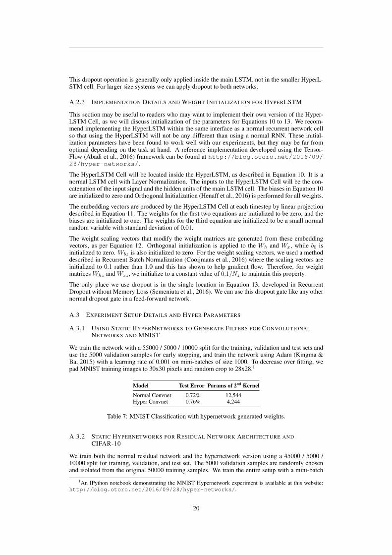
We start by applying a hypernetwork to generate the filters for a convolutional network on MNIST.Our main convolutional network is a small two layer network and the hypernetwork is used to gener-ate the kernel for the second layer (7x7x16x16), which contains the bulk of the trainable parametersin the system. Our weight matrix will be summarized by an embedding of size Nz = 4. SeeAppendix A.3.1 for further experimental setup details.

For this task, the hypernetwork achieved a test accuracy of 99.24%, comparable to the 99.28% forthe conventional method. In this example, a kernel consisting of 12,544 weights is represented by anembedding vector of only 4 parameters, generated by a hypernetwork that has 4240 parameters. Wecan see the weight matrix this network produced by the hypernetwork in Figure 2. Now the questionis whether we can also train a deep convolutional network, using a single hypernetwork generatinga set of weights for each layer, on a dataset more challenging than MNIST.

4.2 STATIC HYPERNETWORKS FOR RESIDUAL NETWORK ARCHITECTURE AND CIFAR-10

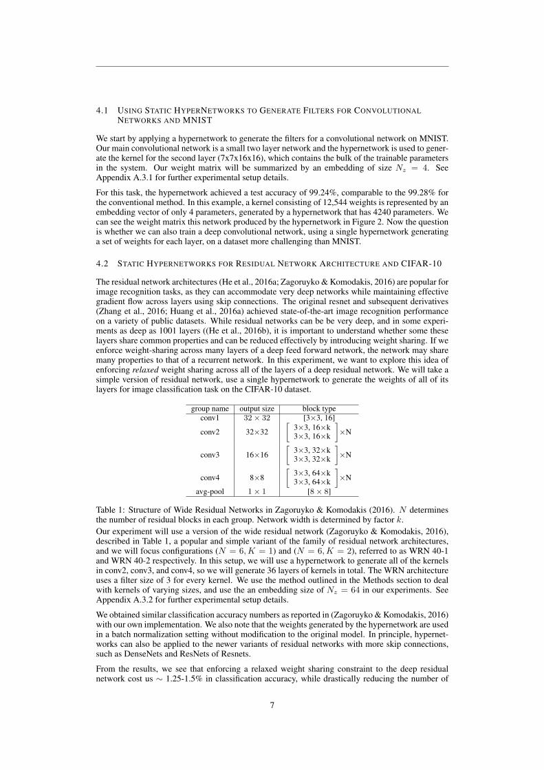
The residual network architectures (He et al., 2016a; Zagoruyko & Komodakis, 2016) are popular forimage recognition tasks, as they can accommodate very deep networks while maintaining effectivegradient flow across layers using skip connections. The original resnet and subsequent derivatives(Zhang et al., 2016; Huang et al., 2016a) achieved state-of-the-art image recognition performanceon a variety of public datasets. While residual networks can be be very deep, and in some experi-ments as deep as 1001 layers ((He et al., 2016b), it is important to understand whether some theselayers share common properties and can be reduced effectively by introducing weight sharing. If weenforce weight-sharing across many layers of a deep feed forward network, the network may sharemany properties to that of a recurrent network. In this experiment, we want to explore this idea ofenforcing relaxed weight sharing across all of the layers of a deep residual network. We will take asimple version of residual network, use a single hypernetwork to generate the weights of all of itslayers for image classification task on the CIFAR-10 dataset.

group name output size block typeconv1 32× 32 [3×3, 16]

conv2 32×32[

3×3, 16×k3×3, 16×k

]×N

conv3 16×16[

3×3, 32×k3×3, 32×k

]×N

conv4 8×8[

3×3, 64×k3×3, 64×k

]×N

avg-pool 1× 1 [8× 8]

Table 1: Structure of Wide Residual Networks in Zagoruyko & Komodakis (2016). N determinesthe number of residual blocks in each group. Network width is determined by factor k.Our experiment will use a version of the wide residual network (Zagoruyko & Komodakis, 2016),described in Table 1, a popular and simple variant of the family of residual network architectures,and we will focus configurations (N = 6,K = 1) and (N = 6,K = 2), referred to as WRN 40-1and WRN 40-2 respectively. In this setup, we will use a hypernetwork to generate all of the kernelsin conv2, conv3, and conv4, so we will generate 36 layers of kernels in total. The WRN architectureuses a filter size of 3 for every kernel. We use the method outlined in the Methods section to dealwith kernels of varying sizes, and use the an embedding size of Nz = 64 in our experiments. SeeAppendix A.3.2 for further experimental setup details.

We obtained similar classification accuracy numbers as reported in (Zagoruyko & Komodakis, 2016)with our own implementation. We also note that the weights generated by the hypernetwork are usedin a batch normalization setting without modification to the original model. In principle, hypernet-works can also be applied to the newer variants of residual networks with more skip connections,such as DenseNets and ResNets of Resnets.

From the results, we see that enforcing a relaxed weight sharing constraint to the deep residualnetwork cost us ∼ 1.25-1.5% in classification accuracy, while drastically reducing the number of

7

Model Test Error Param Count

Network in Network (Lin et al., 2014) 8.81%FitNet (Romero et al., 2014) 8.39%Deeply Supervised Nets (Lee et al., 2015) 8.22%Highway Networks (Srivastava et al., 2015) 7.72%ELU (Clevert et al., 2015) 6.55%Original Resnet-110 (He et al., 2016a) 6.43% 1.7 MStochastic Depth Resnet-110 (Huang et al., 2016b) 5.23% 1.7 MWide Residual Network 40-1 (Zagoruyko & Komodakis, 2016) 6.85% 0.6 MWide Residual Network 40-2 (Zagoruyko & Komodakis, 2016) 5.33% 2.2 MWide Residual Network 28-10 (Zagoruyko & Komodakis, 2016) 4.17% 36.5 MResNet of ResNet 58-4 (Zhang et al., 2016) 3.77% 13.3 MDenseNet (Huang et al., 2016a) 3.74% 27.2 M

Wide Residual Network 40-12 6.73% 0.563 MHyper Residual Network 40-1 (ours) 8.02% 0.097 MWide Residual Network 40-22 5.66% 2.236 MHyper Residual Network 40-2 (ours) 7.23% 0.148 M

Table 2: CIFAR-10 Classification with hypernetwork generated weights.

parameters in the model as a trade off. One reason for this reduction in accuracy is because differentlayers of a deep network is trained to extract different levels of features, and require different kindsof filters to perform optimally. The hypernetwork enforces some commonality between every layer,but offers each layer 64 degrees of freedom to distinguish itself from the other layers. While thenetwork is no longer able to learn the optimal set of filters for each layer, it will learn the best set offilters given the constraints, and the resulting number of model parameters is drastically reduced.

4.3 HYPERLSTM FOR CHARACTER-LEVEL PENN TREEBANK LANGUAGE MODELLING

The HyperLSTM model is evaluated on character level prediction task on the Penn Treebank corpus(Marcus et al., 1993) using the train/validation/test split outlined in (Mikolov et al., 2012). As thedataset is quite small is prone to over fitting, we apply dropout on both input and output layers witha keep probability of 0.90. Unlike previous approaches (Graves, 2013; Ognawala & Bayer, 2014) ofapplying weight noise during training, we instead also apply dropout to the recurrent layer (Henaffet al., 2016) with the same dropout probability.

We compare our model to the basic LSTM cell, stacked LSTM cells (Graves, 2013), and LSTM withlayer normalization applied. In addition, we also experimented with applying layer normalizationto HyperLSTM. Using the setup in (Graves, 2013), we use networks with 1000 units and train thenetwork to predict the next character. In this task, the HyperLSTM cell has 128 units and a signalsize of 4. As the HyperLSTM cell has more trainable parameters compared to the basic LSTMCell, we also experimented with an LSTM Cell with 1250 units as well. For more details regardingexperimental setup, please refer to Appendix A.3.3

It is interesting to note that combining Recurrent Dropout with a basic LSTM cell achieves quiteformidable performance. Our implementation of Recurrent Dropout Basic LSTM cell reproducedsimilar results as (Semeniuta et al., 2016), where they have also experimented with different dropoutsettings. We also found that Layer Norm LSTM performed quite well when combined with recurrentdropout, making it both a formidable baseline and also an extension for HyperLSTM.

In addition to outperforming both the larger or deeper version of the LSTM network, HyperLSTMalso achieved similar performance of Layer Norm LSTM. This suggests by dynamically adjustingthe weight scaling vectors, the HyperLSTM cell has learned a policy of scaling inputs to the ac-tivation functions that is as efficient as the statistical moments-based strategy employed by LayerNorm, and that the required extra computation required is embedded inside the extra 128 units in-side the HyperLSTM cell. When we combine HyperLSTM with Layer Norm, we see an additionalperformance gain, implying that the HyperLSTM cell learned an adjustment policy that goes be-yond moments-based regularization. We also demonstrate that increasing the size of the embeddingvector or stacking HyperLSTM layers together can also increase its performance.

8

Model1 Test Validation Param Count

ME n-gram (Mikolov et al., 2012) 1.37Batch Norm LSTM (Cooijmans et al., 2016) 1.32Recurrent Dropout LSTM (Semeniuta et al., 2016) 1.301 1.338Zoneout RNN (Krueger et al., 2016) 1.27HM-LSTM3 (Chung et al., 2016) 1.27

LSTM, 1000 units 2 1.312 1.347 4.25 MLSTM, 1250 units2 1.306 1.340 6.57 M2-Layer LSTM, 1000 units2 1.281 1.312 12.26 MLayer Norm LSTM, 1000 units2 1.267 1.300 4.26 MHyperLSTM (ours), 1000 units 1.265 1.296 4.91 MLayer Norm HyperLSTM, 1000 units (ours) 1.250 1.281 4.92 MLayer Norm HyperLSTM, 1000 units, Large Embedding (ours) 1.233 1.263 5.06 M2-Layer Norm HyperLSTM, 1000 units 1.219 1.245 14.41 M

Table 3: Bits-per-character on the Penn Treebank test set.

4.4 HYPERLSTM FOR HUTTER PRIZE WIKIPEDIA LANGUAGE MODELLING

We train our model on the larger and more challenging Hutter Prize Wikipedia dataset, also knownas enwik8 (Hutter, 2012) consisting of a sequence of 100M characters composed of 205 uniquecharacters. Unlike Penn Treebank, enwik8 contains some foreign words (Latin, Arabic, Chinese),indented XML, metadata, and internet addresses, making it a more realistic and practical datasetto test character language models. For more details regarding experimental setup, please refer toAppendix A.3.4. Examples of these mixed variety of text samples that our HyperLSTM model cangenerate is in Appendix A.4.

Model1 enwik8 Param Count

Stacked LSTM (Graves, 2013) 1.67 27.0 MMRNN (Sutskever et al., 2011) 1.60GF-RNN (Chung et al., 2015) 1.58 20.0 MGrid-LSTM (Kalchbrenner et al., 2016) 1.47 16.8 MLSTM (Rocki, 2016b) 1.45MI-LSTM (Wu et al., 2016) 1.44Recurrent Highway Networks (Zilly et al., 2016) 1.42 8.0 MRecurrent Memory Array Structures (Rocki, 2016a) 1.40HM-LSTM3 (Chung et al., 2016) 1.40Surprisal Feedback LSTM4 (Rocki, 2016b) 1.37

LSTM, 1800 units, no recurrent dropout2 1.470 14.81 MLSTM, 2000 units, no recurrent dropout2 1.461 18.06 MLayer Norm LSTM, 1800 units2 1.402 14.82 MHyperLSTM (ours), 1800 units 1.391 18.71 MLayer Norm HyperLSTM, 1800 units (ours) 1.353 18.78 MLayer Norm HyperLSTM, 2048 units (ours) 1.340 26.54 M

Table 4: Bits-per-character on the enwik8 test set.

We see that HyperLSTM is once again competitive to Layer Norm LSTM, and if we combine bothtechniques, the Layer Norm HyperLSTM achieves respectable results. The version of HyperLSTMthat uses 2048 hidden units achieve near state-of-the-art performance for this task. In addition,HyperLSTM converges quicker per training step compared to LSTM and Layer Norm LSTM. Pleaserefer to Figure 6 for the loss graphs.

1We do not compare against methods that use dynamic evaluation.2Our implementation.3Based on results of version 2 at the time of writing. http://arxiv.org/abs/1609.01704v24This method uses information about test errors during inference for predicting the next characters, hence

it is not directly comparable to other methods that do not use this information.

9

 In 1955-37 most American and Europeans signed into the sea. An absence of [[Japan (Korea city)|Japan]], the Mayotte like Constantino In 1955-37 most American and Europeans signed into the sea. An absence of [[Japan (Korea city)|Japan]], the Mayotte like Constantino

 ple (in its first week, in [[880]]) that served as the mother of emperors, as the Corinthians, Bernard on his continued sequel toget ple (in its first week, in [[880]]) that served as the mother of emperors, as the Corinthians, Bernard on his continued sequel toget

 her ordered [[Operation Moabili]]. The Gallup churches in the army promulgated the possessions sitting at the reservation, and [[Mel her ordered [[Operation Moabili]]. The Gallup churches in the army promulgated the possessions sitting at the reservation, and [[Mel

 ito de la Vegeta Provine|Felix]] had broken Diocletian desperate from the full victory of Augustus, cited by Stephen I. Alexander Se ito de la Vegeta Provine|Felix]] had broken Diocletian desperate from the full victory of Augustus, cited by Stephen I. Alexander Se

 nate became Princess Cartara, an annual ruler of war (777-184) and founded numerous extremiti of justice practitioners. nate became Princess Cartara, an annual ruler of war (777-184) and founded numerous extremiti of justice practitioners.

Figure 4: Example text generated from HyperLSTM model. We visualize how four of the mainRNN’s weight matrices (W i

h, W gh , W f

h , W oh ) effectively change over time by plotting the norm of

the changes below each generated character. High intensity represent large changes being made toweights of main RNN.

When we use this prediction model as a generative model to sample a text passage, we use mainRNN to model a probability distribution over possible characters conditioned over the precedingcharacters. In the case of the HyperRNN, we allow the model parameters of this generative modelto vary over time, so in effect the HyperRNN cell is choosing the best model at any given time togenerate a probability distribution to sample from. We can demonstrate this by visualizing how theweight scaling vectors of the main RNN change during the character sampling process. In Figure 4,we examine a sample text passage generated by HyperLSTM after training on enwik8 along withthe weight differences below the text. We see that in regions of low intensity, where the weightsof the main RNN are relatively static, the types of phrases generated seem more deterministic. Forexample, the weights do not change much during the words Europeans, possessions andreservation. The regions of high intensity is when the HyperRNN cell is making relativelylarge changes to the weights of the main RNN. These tend to happen in the areas between words, orsometimes during brackets.

One might also wonder whether the HyperLSTM cell (without Layer Norm), via dynamically tuningthe weight scaling vectors, has developed a policy that is similar to the statistics-based approach usedby Layer Norm, given that both methods have similar performance. One way to see this effect is tolook at the histogram of the hidden states in the network. In Figure 5, we examine the histograms ofφ(ct), the hidden state of the LSTM before applying the output gate.

Figure 5: Normalized Histogram plots of φ(ct) for different models during sampling.

We see that the normalization process employed by Layer Norm reduces the saturation effects com-pared to the vanilla LSTM. However, for the case of the HyperLSTM, we notice that most of thetime the cell is saturated. The HyperLSTM cell’s dynamic weight adjustment policy appears to bedoing something very different compared to statistical normalization, although the policy it came upwith ended up providing similar performance as Layer Norm. It is interesting to see that when wecombine both methods, the HyperLSTM cell will need to determine an adjustment policy in spiteof the normalization forced upon it by Layer Norm. An interesting question is whether there areproblems where statistical normalization may actually be a setback to the policy developed by theHyperLSTM, and the best strategy is to ignore it.

10

Figure 6: Loss Graph for enwik8 (left). Loss Graph for Handwriting Generation (right)

4.5 HYPERLSTM FOR HANDWRITING SEQUENCE GENERATION

In addition to modelling discrete sequential data, we want to see how the model performs whenmodelling sequences of real valued data. We will train our model on the IAM online handwrit-ing database (Liwicki & Bunke, 2005) and have our model predict pen strokes as per Section 4.2of (Graves, 2013). The dataset has contains 12179 handwritten lines from 221 writers, digitallyrecorded from a tablet. We will model the (x, y) coordinate of the pen location at each recordedtime step, along with a binary indicator of pen-up/pen-down. The average sequence length is around700 steps and the longest around 1900 steps, making the training task particularly challenging as thenetwork needs to retain information about both the stroke history and also the handwriting style inorder to predict plausible future handwriting strokes. For experimental setup details, please refer toAppendix A.3.5.

Model Log-Loss Param Count

LSTM, 900 units (Graves, 2013) -1,0263-Layer LSTM, 400 units (Graves, 2013) -1,0413-Layer LSTM, 400 units, adaptive weight noise (Graves, 2013) -1,058

LSTM, 900 units, no dropout, no data augmentation.1 -1,026 3.36 M3-Layer LSTM, 400 units, no dropout, no data augmentation.1 -1,039 3.26 M

LSTM, 900 units2 -1,055 3.36 MLSTM, 1000 units2 -1,048 4.14 M3-Layer LSTM, 400 units2 -1,068 3.26 M2-Layer LSTM, 650 units2 -1,135 5.16 MLayer Norm LSTM, 900 units2 -1,096 3.37 MLayer Norm LSTM, 1000 units2 -1,106 4.14 MLayer Norm HyperLSTM, 900 units (ours) -1,067 3.95 MHyperLSTM (ours), 900 units -1,162 3.94 M

Table 5: Log-Loss of IAM Online DB validation set.

In this task, we note that data augmentation and applying recurrent dropout improved the perfor-mance of all models, compared to the original setup by (Graves, 2013). In addition, for the LSTMmodel, increasing unit count per layer may not help the performance compared to increasing thelayer depth. We notice that a 3-layer 400 unit LSTM outperforms a 1-layer 900 unit one, and wefound that a 2-layer 650 unit LSTM outperforming most configurations. While layer norm helpswith the performance, we found that in this task, layer norm does not combine well with HyperL-STM, and in this task the 900 unit HyperLSTM without layer norm achieved the best performance.

Unlike the language modelling task, perhaps statistical normalization is far from the optimal ap-proach for a weight adjustment policy. The policy learned by the HyperLSTM cell not only per-

1Our implementation, to replicate setup of (Graves, 2013).2Our implementation, with data augmentation, dropout and recurrent dropout.

11

formed well against the baseline, its convergence rate is also as fast as the 2-layer LSTM model.Please refer to Figure 6 for the loss graphs.

In Appendix A.5, we display three sets of handwriting samples generated from LSTM, Layer NormLSTM, and HyperLSTM, corresponding to log-loss scores of -1055, -1096, and -1162 nats respec-tively in Table 5. Qualitative assessments of handwriting quality is always subjective, and dependsan individual’s taste in calligraphy. From looking at the examples produced by the three models, ouropinion is that the samples produced by LSTM is noisier than the other two models. We also findHyperLSTM’s samples to be a bit more coherent than the samples produced by Layer Norm LSTM.We leave to the reader to judge which model produces handwriting samples of higher quality.

Figure 7: Handwriting sample generated from HyperLSTM model. We visualize how four of themain RNN’s weight matrices (W i

h Wgh , W f

h , W oh ) effectively change over time, by plotting norm of

changes made to them over time.

Similar to the earlier character generation experiment, we show a generated handwriting samplefrom the HyperLSTM model in Figure 7, along with a plot of how the weight scaling vectors of themain RNN is changing over time below the sample. For a more detailed interactive demonstration ofhandwriting generation using HyperLSTM, visit http://blog.otoro.net/2016/09/28/hyper-networks/.

We see that the regions of high intensity seem to be concentrated at many discrete instances, ratherthan slowly varying over time. This implies that the weights experience regime changes ratherthan gradual slow adjustments. We can see that many of these weight changes occur between thewritten words, and sometimes between written characters. While the LSTM model alone alreadydoes a formidable job of generating time-varying parameters of a Mixture Gaussian distributionused to generate realistic handwriting samples, the ability to go one level deeper, and to dynamicallygenerate the generative model is one of the key advantages of HyperRNN over a normal RNN.

4.6 HYPERLSTM FOR NEURAL MACHINE TRANSLATION

We experiment with the Neural Machine Translation task using the same experimental setup outlinedin (Wu et al., 2016). Our model is the same wordpiece model architecture with a vocabulary size of32k, but we replace the LSTM cells with HyperLSTM cells. We benchmark the modified model onWMT’14 En→Fr using the same test/validation set split described in the GNMT paper (Wu et al.,2016). Please refer to Appendix A.3.6 for experimental setup details.

Model Test BLEU Log Perplexity

Deep-Att + PosUnk (Zhou et al., 2016) 39.2GNMT WPM-32K, LSTM (Wu et al., 2016) 38.95 1.027GNMT WPM-32K, ensemble of 8 LSTMs (Wu et al., 2016) 40.35

GNMT WPM-32K, HyperLSTM (ours) 40.03 0.993

Table 6: Single model results on WMT En→Fr (newstest2014)

The HyperLSTM cell improves the performance of the existing GNMT model, achieving state-of-the-art single model results for this dataset. In addition, we demonstrate the applicability ofhypernetworks to large-scale models used in production systems. Please see Appendix A.6 foractual translation samples generated from both models for a qualitative comparison.

12

5 CONCLUSION

In this paper, we presented a method to use a hypernetwork to generate weights for another neuralnetwork. Our hypernetworks are trained end-to-end with backpropagation and therefore are effi-cient and scalable. We focused on two use cases of hypernetworks: static hypernetworks to generateweights for a convolutional network, dynamic hypernetworks to generate weights for recurrent net-works. We found that the method works well while using fewer parameters. On image recognition,language modelling and handwriting generation, hypernetworks are competitive to or sometimesbetter than state-of-the-art models.

ACKNOWLEDGMENTS

We thank Jeff Dean, Geoffrey Hinton, Mike Schuster and the Google Brain team for their help withthe project.

REFERENCES

Martín Abadi, Ashish Agarwal, Paul Barham, Eugene Brevdo, Zhifeng Chen, Craig Citro, Gre-gory S. Corrado, Andy Davis, Jeffrey Dean, Matthieu Devin, Sanjay Ghemawat, Ian J. Good-fellow, Andrew Harp, Geoffrey Irving, Michael Isard, Yangqing Jia, Rafal Józefowicz, LukaszKaiser, Manjunath Kudlur, Josh Levenberg, Dan Mané, Rajat Monga, Sherry Moore, Derek Gor-don Murray, Chris Olah, Mike Schuster, Jonathon Shlens, Benoit Steiner, Ilya Sutskever, KunalTalwar, Paul A. Tucker, Vincent Vanhoucke, Vijay Vasudevan, Fernanda B. Viégas, Oriol Vinyals,Pete Warden, Martin Wattenberg, Martin Wicke, Yuan Yu, and Xiaoqiang Zheng. Tensorflow:Large-scale machine learning on heterogeneous distributed systems. CoRR, abs/1603.04467,2016. URL http://arxiv.org/abs/1603.04467.

M. Andrychowicz, M. Denil, S. Gomez, M. W. Hoffman, D. Pfau, T. Schaul, and N. de Freitas.Learning to learn by gradient descent by gradient descent. arXiv preprint arXiv:1606.04474,2016.

Jimmy L. Ba, Jamie R. Kiros, and Geoffrey E. Hinton. Layer normalization. NIPS, 2016.

Luca Bertinetto, João F. Henriques, Jack Valmadre, Philip H. S. Torr, and Andrea Vedaldi. Learningfeed-forward one-shot learners. In NIPS, 2016.

Christopher M. Bishop. Mixture density networks. Technical report, 1994.

Junyoung Chung, Caglar Gülçehre, Kyunghyun Cho, and Yoshua Bengio. Gated feedback recurrentneural networks. arXiv preprint arXiv:1502.02367, 2015.

Junyoung Chung, Sungjin Ahn, and Yoshua Bengio. Hierarchical multiscale recurrent neural net-works. arXiv preprint arXiv:1609.01704, 2016.

Djork-Arné Clevert, Thomas Unterthiner, and Sepp Hochreiter. Fast and accurate deep networklearning by exponential linear units (ELUs). arXiv preprint arXiv:1511.07289, 2015.

Tim Cooijmans, Nicolas Ballas, Cesar Laurent, and Caglar Gulcehre. Recurrent Batch Normaliza-tion. arXiv:1603.09025, 2016.

Bert De Brabandere, Xu Jia, Tinne Tuytelaars, and Luc Van Gool. Dynamic filter networks. InNIPS, 2016.

Misha Denil, Babak Shakibi, Laurent Dinh, Marc’Aurelio Ranzato, and Nando de Freitas. PredictingParameters in Deep Learning. In NIPS, 2013.

Chrisantha Fernando, Dylan Banarse, Malcolm Reynolds, Frederic Besse, David Pfau, Max Jader-berg, Marc Lanctot, and Daan Wierstra. Convolution by evolution: Differentiable pattern produc-ing networks. In GECCO, 2016.

Faustino Gomez and Jürgen Schmidhuber. Evolving modular fast-weight networks for control. InICANN, 2005.

13

Alex Graves. Generating sequences with recurrent neural networks. arXiv:1308.0850, 2013.

Kaiming He, Xiangyu Zhang, Shaoqing Ren, and Jian Sun. Deep residual learning for image recog-nition. In CVPR, 2016a.

Kaiming He, Xiangyu Zhang, Shaoqing Ren, and Jian Sun. Identity mappings in deep residualnetworks. arXiv preprint arXiv:1603.05027, 2016b.

Mikael Henaff, Arthur Szlam, and Yann LeCun. Orthogonal RNNs and long-memory tasks. InICML, 2016.

Geoffrey E Hinton, Nitish Srivastava, Alex Krizhevsky, Ilya Sutskever, and Ruslan R Salakhutdi-nov. Improving neural networks by preventing co-adaptation of feature detectors. arXiv preprintarXiv:1207.0580, 2012.

Sepp Hochreiter and Juergen Schmidhuber. Long short-term memory. Neural Computation, 1997.

Gao Huang, Zhuang Liu, and Kilian Q. Weinberger. Densely connected convolutional networks.arXiv preprint arXiv:1608.06993, 2016a.

Gao Huang, Yu Sun, Zhuang Liu, Daniel Sedra, and Kilian Weinberger. Deep networks with stochas-tic depth. arXiv preprint arXiv:1603.09382, 2016b.

Marcus Hutter. The human knowledge compression contest. 2012. URL http://prize.hutter1.net/.

Max Jaderberg, Wojciech Marian Czarnecki, Simon Osindero, Oriol Vinyals, Alex Graves, andKoray Kavukcuoglu. Decoupled Neural Interfaces using Synthetic Gradients. arXiv preprintarXiv:1608.05343, 2016.

Nal Kalchbrenner, Ivo Danihelka, and Alex Graves. Grid long short-term memory. In ICLR, 2016.

Diederik Kingma and Jimmy Ba. Adam: A method for stochastic optimization. In ICLR, 2015.

Jan Koutnik, Faustino Gomez, and Jürgen Schmidhuber. Evolving neural networks in compressedweight space. In GECCO, 2010.

David Krueger, Tegan Maharaj, János Kramár, Mohammad Pezeshki, Nicolas Ballas, Nan RosemaryKe, Anirudh Goyal, Yoshua Bengio, Hugo Larochelle, Aaron Courville, et al. Zoneout: Regular-izing RNNs by randomly preserving hidden activations. arXiv preprint arXiv:1606.01305, 2016.

Y. LeCun, B. Boser, J. S. Denker, D. Henderson, R. E. Howard, W. Hubbard, and L. D. Jackel.Handwritten digit recognition with a back-propagation network. In NIPS, 1990.

Chen-Yu Lee, Saining Xie, Patrick Gallagher, Zhengyou Zhang, and Zhuowen Tu. Deeply-supervised nets. In AISTATS, volume 2, pp. 6, 2015.

Min Lin, Qiang Chen, and Shuicheng Yan. Network in network. In ICLR, 2014.

Marcus Liwicki and Horst Bunke. IAM-OnDB - an on-line English sentence database acquired fromhandwritten text on a whiteboard. In ICDAR, 2005.

Mitchell P. Marcus, Mary Ann Marcinkiewicz, and Beatrice Santorini. Building a large annotatedcorpus of english: The penn treebank. Computational linguistics, 19(2):313–330, 1993.

Tomáš Mikolov, Ilya Sutskever, Anoop Deoras, Hai-Son Le, Stefan Kombrink, and Jan Cernocky.Subword language modeling with neural networks. preprint, 2012.

Marcin Moczulski, Misha Denil, Jeremy Appleyard, and Nando de Freitas. ACDC: A StructuredEfficient Linear Layer. arXiv preprint arXiv:1511.05946, 2015.

Saahil Ognawala and Justin Bayer. Regularizing recurrent networks-on injected noise and norm-based methods. arXiv preprint arXiv:1410.5684, 2014.

Kamil Rocki. Recurrent memory array structures. arXiv preprint arXiv:1607.03085, 2016a.

14

Kamil Rocki. Surprisal-driven feedback in recurrent networks. arXiv preprint arXiv:1608.06027,2016b.

Adriana Romero, Nicolas Ballas, Samira Ebrahimi Kahou, Antoine Chassang, Carlo Gatta, andYoshua Bengio. Fitnets: Hints for thin deep nets. arXiv preprint arXiv:1412.6550, 2014.

Jürgen Schmidhuber. Learning to control fast-weight memories: An alternative to dynamic recurrentnetworks. Neural Computation, 4(1):131–139, 1992.

Jürgen Schmidhuber. A ‘self-referential’ weight matrix. In ICANN, 1993.

Stanislaw Semeniuta, Aliases Severyn, and Erhardt Barth. Recurrent dropout without memory loss.arXiv:1603.05118, 2016.

Rupesh Srivastava, Klaus Greff, and Jürgen Schmidhuber. Training very deep networks. In NIPS,2015.

Kenneth O. Stanley, David B. D’Ambrosio, and Jason Gauci. A hypercube-based encoding forevolving large-scale neural networks. Artificial Life, 15(2):185–212, 2009.

Ilya Sutskever, James Martens, and Geoffrey E. Hinton. Generating text with recurrent neural net-works. In ICML, 2011.

Y. Wu, M. Schuster, Z. Chen, Q. V. Le, M. Norouzi, W. Macherey, M. Krikun, Y. Cao, Q. Gao,K. Macherey, J. Klingner, A. Shah, M. Johnson, X. Liu, Ł. Kaiser, S. Gouws, Y. Kato, T. Kudo,H. Kazawa, K. Stevens, G. Kurian, N. Patil, W. Wang, C. Young, J. Smith, J. Riesa, A. Rudnick,O. Vinyals, G. Corrado, M. Hughes, and J. Dean. Google’s Neural Machine Translation System:Bridging the Gap between Human and Machine Translation. ArXiv e-prints, 2016.

Yuhuai Wu, Saizheng Zhang, Ying Zhang, Yoshua Bengio, and Ruslan Salakhutdinov. On multi-plicative integration with recurrent neural networks. NIPS, 2016.

Jianlin Xia, Shivkumar Chandrasekaran, Ming Gu, and Xiaoye S. Li. Fast algorithms for hierarchi-cally semiseparable matrices. Numerical Linear Algebra with Applications, 2010.

Z. Yang, M. Moczulski, M. Denil, N. de Freitas, A. Smola, L. Song, and Z. Wang. Deep FriedConvnets. In ICCV, 2015.

Sergey Zagoruyko and Nikos Komodakis. Wide residual networks. In BMVC, 2016.

Ke Zhang, Miao Sun, Tony X. Han, Xingfang Yuan, Liru Guo, and Tao Liu. Residual networks ofresidual networks: Multilevel residual networks. arXiv preprint arXiv:1608.02908, 2016.

Jie Zhou, Ying Cao, Xuguang Wang, Peng Li, and Wei Xu. Deep recurrent models with fast-forward connections for neural machine translation. CoRR, abs/1606.04199, 2016. URL http://arxiv.org/abs/1606.04199.

Julian Zilly, Rupesh Srivastava, Jan Koutník, and Jürgen Schmidhuber. Recurrent highway networks.arXiv preprint arXiv:1607.03474, 2016.

15

A APPENDIX

A.1 HYPERNETWORKS TO LEARN FILTERS FOR A FULLY CONNECTED NETWORKS

Figure 8: Filters learned to classify MNIST digits in a fully connected network (left). Filters learnedby a hypernetwork (right).

We ran an experiment where the hypernetwork receives the x, y locations of both the input pixeland the weight, and predicts the value of the hidden weight matrix in a fully connected network thatlearns to classify MNIST digits. In this experiment, the fully connected network (784-256-10) hasone hidden layer of 16 × 16 units, where the hypernetwork is a pre-defined small feedforward net-work. The weights of the hidden layer has 784×256 = 200704 parameters, while the hypernetworkis a 801 parameter four layer feed forward relu network that would generate the 786 × 256 weightmatrix. The result of this experiment is shown in Figure 8. We want to emphasize that even thoughthe network can learn convolutional-like filters during end-to-end training, its performance is ratherpoor: the best accuracy is 93.5%, compared to 98.5% for the conventional fully connected network.

We find that the virtual coordinates-based approach to hypernetworks that is used by HyperNEATand DPPN has its limitations in many practical tasks, such as image recognition and language mod-elling, and therefore developed our embedding vector approach in this work.

16

A.2 CONCEPTUAL DIAGRAMS OF STATIC AND DYNAMIC HYPERNETWORKS

Figure 9: Feedforward Network (top) and Recurrent Network (bottom)

Figure 10: Static Hypernetwork generating weights for Feedforward Network

Figure 11: Dynamic Hypernetwork generating weights for Recurrent Network

17

A.2.1 FILTER VISUALIZATIONS FOR RESIDUAL NETWORKS

In Figures 12 and 13 are example visualizations for various kernels in a deep residual network. Notethat the 32x32x3x3 kernel generated by the hypernetwork was constructed by concatenating 4 basickernels together.

Figure 12: Normal CIFAR-10 16x16x3x3 kernel (left). Normal CIFAR-10 32x32x3x3 kernel (right).

Figure 13: Generated 16x16x3x3 kernel (left). Generated 32x32x3x3 kernel (right).

18

A.2.2 HYPERLSTM

In this section we will discuss extension of HyperRNN to LSTM. Our focus will be on the basicversion of the LSTM architecture Hochreiter & Schmidhuber (1997), given by:

it =W ihht−1 +W i

xxt + bi

gt =W ghht−1 +W g

xxt + bg

ft =W fh ht−1 +W f

x xt + bf

ot =W ohht−1 +W o

xxt + bo

ct = σ(ft)� ct−1 + σ(it)� φ(gt)ht = σ(ot)� φ(ct)

(9)

where W yh ∈ RNh×Nh ,W y

x ∈ RNh×Nx , by ∈ RNh , σ is the sigmoid operator, φ is the tanhoperator. For brevity, y is one of {i, g, f, o}.1

Similar to the previous section, we will make the weights and biases a function of an embedding, andthe embedding for each {i, g, f, o} will be generated from a smaller HyperLSTM cell. As discussedearlier, we will also experiment with adding the option to use a Layer Normalization layer in theHyperLSTM. The HyperLSTM Cell is given by:

xt =

(ht−1

xt

)

it = LN(W ihht−1 +W i

xxt + bi)

gt = LN(W g

hht−1 +W g

x xt + bg)

ft = LN(W f

hht−1 +W f

x xt + bf )

ot = LN(W ohht−1 +W o

x xt + bo)

ct = σ(ft)� ct−1 + σ(it)� φ(gt)ht = σ(ot)� φ(LN(ct))

(10)

The weight matrices for each of the four {i, g, f, o} gates will be a function of a set of embeddingszx, zh, and zb unique to each gates, just like the HyperRNN. These embeddings are linear projectionsof the hidden states of the HyperLSTM Cell. For brevity, y is one of {i, g, f, o} to avoid writingfour sets of identical equations:

zyh =W y

hhht−1 + by

hh

zyx =W y

hxht−1 + by

hx

zyb =W y

hbht−1

(11)

As in the memory efficient version of the HyperRNN, we will focus on the efficient version of theHyperLSTM, where we use weight scaling vectors d to modify the rows of the weight matrices:

yt = LN(dyh �W

yhht−1 + dyx �W y

xxt + by(zyb )), where

dyh(zh) =W yhzzh

dyx(zx) =W yxzzx

by(zyb ) =W ybzz

yb + by0

(12)

In our implementation, the cell and hidden state update equations for the main LSTM will incorpo-rate a single dropout (Hinton et al., 2012) gate, as developed in Recurrent Dropout without MemoryLoss (Semeniuta et al., 2016), as we found this to help regularize the entire model during training:

ct = σ(ft)� ct−1 + σ(it)�DropOut(φ(gt))ht = σ(ot)� φ(LN(ct))

(13)

1In practice, all eight weight matrices are concatenated into one large matrix for computational efficiency.

19

This dropout operation is generally only applied inside the main LSTM, not in the smaller HyperL-STM cell. For larger size systems we can apply dropout to both networks.

A.2.3 IMPLEMENTATION DETAILS AND WEIGHT INITIALIZATION FOR HYPERLSTM

This section may be useful to readers who may want to implement their own version of the Hyper-LSTM Cell, as we will discuss initialization of the parameters for Equations 10 to 13. We recom-mend implementing the HyperLSTM within the same interface as a normal recurrent network cellso that using the HyperLSTM will not be any different than using a normal RNN. These initial-ization parameters have been found to work well with our experiments, but they may be far fromoptimal depending on the task at hand. A reference implementation developed using the Tensor-Flow (Abadi et al., 2016) framework can be found at http://blog.otoro.net/2016/09/28/hyper-networks/.

The HyperLSTM Cell will be located inside the HyperLSTM, as described in Equation 10. It is anormal LSTM cell with Layer Normalization. The inputs to the HyperLSTM Cell will be the con-catenation of the input signal and the hidden units of the main LSTM cell. The biases in Equation 10are initialized to zero and Orthogonal Initialization (Henaff et al., 2016) is performed for all weights.

The embedding vectors are produced by the HyperLSTM Cell at each timestep by linear projectiondescribed in Equation 11. The weights for the first two equations are initialized to be zero, and thebiases are initialized to one. The weights for the third equation are initialized to be a small normalrandom variable with standard deviation of 0.01.

The weight scaling vectors that modify the weight matrices are generated from these embeddingvectors, as per Equation 12. Orthogonal initialization is applied to the Wh and Wx, while b0 isinitialized to zero. Wbz is also initialized to zero. For the weight scaling vectors, we used a methoddescribed in Recurrent Batch Normalization (Cooijmans et al., 2016) where the scaling vectors areinitialized to 0.1 rather than 1.0 and this has shown to help gradient flow. Therefore, for weightmatrices Whz and Wxz , we initialize to a constant value of 0.1/Nz to maintain this property.

The only place we use dropout is in the single location in Equation 13, developed in RecurrentDropout without Memory Loss (Semeniuta et al., 2016). We can use this dropout gate like any othernormal dropout gate in a feed-forward network.

A.3 EXPERIMENT SETUP DETAILS AND HYPER PARAMETERS

A.3.1 USING STATIC HYPERNETWORKS TO GENERATE FILTERS FOR CONVOLUTIONALNETWORKS AND MNIST

We train the network with a 55000 / 5000 / 10000 split for the training, validation and test sets anduse the 5000 validation samples for early stopping, and train the network using Adam (Kingma &Ba, 2015) with a learning rate of 0.001 on mini-batches of size 1000. To decrease over fitting, wepad MNIST training images to 30x30 pixels and random crop to 28x28.1

Model Test Error Params of 2nd Kernel

Normal Convnet 0.72% 12,544Hyper Convnet 0.76% 4,244

Table 7: MNIST Classification with hypernetwork generated weights.

A.3.2 STATIC HYPERNETWORKS FOR RESIDUAL NETWORK ARCHITECTURE ANDCIFAR-10

We train both the normal residual network and the hypernetwork version using a 45000 / 5000 /10000 split for training, validation, and test set. The 5000 validation samples are randomly chosenand isolated from the original 50000 training samples. We train the entire setup with a mini-batch

1An IPython notebook demonstrating the MNIST Hypernetwork experiment is available at this website:http://blog.otoro.net/2016/09/28/hyper-networks/.

20

size of 128 using Nesterov Momentum SGD for the normal version and Adam for the hypernetworkversion, both with a learning rate schedule. We apply L2 regularization on the kernel weights, andalso on the hypernetwork-generated kernel weights of 0.0005%. To decrease over fitting, we applylight data augmentation pad training images to 36x36 pixels and random crop to 32x32, and performrandom horizontal flips.

Table 8: Learning Rate Schedule for Nesterov Momentum SGD

<step learning rate

28,000 0.1000056,000 0.0200084,000 0.00400112,000 0.00080140,000 0.00016

Table 9: Learning Rate Schedule for Hyper Network / Adam

<step learning rate

168,000 0.00200336,000 0.00100504,000 0.00020672,000 0.00005

A.3.3 CHARACTER-LEVEL PENN TREEBANK

The hyper-parameters of all the experiments were selected through non-extensive grid search on thevalidation set. Whenever possible, we used reported learning rates and batch sizes in the literaturethat had been used for similar experiments performed in the past.

For Character-level Penn Treebank, we use mini-batches of size 128, to train on sequences of length100. We trained the model using Adam (Kingma & Ba, 2015) with a learning rate of 0.001 and gra-dient clipping of 1.0. During evaluation, we generate the entire sequence, and do not use informationabout previous test errors for prediction, e.g., dynamic evaluation (Graves, 2013; Rocki, 2016b). Asmentioned earlier, we apply dropout to the input and output layers, and also apply recurrent dropoutwith a keep probability of 90%. For baseline models, Orthogonal Initialization (Henaff et al., 2016)is performed for all weights.

We also experimented with a version of the model using a larger embedding size of 16, and also witha lower dropout keep probability of 85%, and reported results with this “Large Embedding" modelin Table 3. Lastly, we stacked two layers of this “Large Embedding" model together to measure thebenefits of a multi-layer version of HyperLSTM, with a dropout keep probability of 80%.

A.3.4 HUTTER PRIZE WIKIPEDIA

As enwik8 is a bigger dataset compared to Penn Treebank, we will use 1800 units for our networks.In addition, we perform training on sequences of length 250. Our normal HyperLSTM Cell consistsof 256 units, and we use an embedding size of 64.

Our setup is similar in the previous experiment, using the same mini-batch size, learning rate, weightinitialization, gradient clipping parameters and optimizer. We do not use dropout for the input andoutput layers, but still apply recurrent dropout with a keep probability of 90%. For baseline models,Orthogonal Initialization (Henaff et al., 2016) is performed for all weights.

As in (Chung et al., 2015), we train on the first 90M characters of the dataset, use the next 5M as avalidation set for early stopping, and the last 5M characters as the test set.

In this experiment, we also experimented with a slightly larger version of HyperLSTM with 2048hidden units. This version of of the model uses 2048 hidden units for the main network, inline withsimilar models for this experiment in other works. In addition, its HyperLSTM Cell consists of 512

21

units with an embedding size of 64. Given the larger number of nodes in both the main LSTM andHyperLSTM cell, recurrent dropout is also applied to the HyperLSTM Cell of this model, where weuse a lower dropout keep probability of 85%, and train on an increased sequence length of 300.

A.3.5 HANDWRITING SEQUENCE GENERATION

We will use the same model architecture described in (Graves, 2013) and use a Mixture DensityNetwork layer (Bishop, 1994) to generate a mixture of bi-variate Gaussian distributions to model ateach time step to model the pen location. We normalize the data and use the same train/validationsplit as per (Graves, 2013) in this experiment. We remove samples less than length 300 as we foundthese samples contain a lot of recording errors and noise. After the pre-processing, as the dataset issmall, we introduce data augmentation of chosen uniformly from +/- 10% and apply a this randomscaling a the samples used for training.

One concern we want to address is the lack of a test set in the data split methodology devised in(Graves, 2013). In this task, qualitative assessment of generated handwriting samples is arguablyjust as important as the quantitative log likelihood score of the results. Due to the small size of thedataset, we want to use as large as possible the portion of the dataset to train our models in order togenerate better quality handwriting samples so we can also judge our models qualitatively in additionto just examining the log-loss numbers, so for this task we will use the same training / validationsplit as (Graves, 2013), with a caveat that we may be somewhat over fitting to the validation set inthe quantitative results. In future works, we will explore using larger datasets to conduct a morerigorous quantitative analysis.

For model training, will apply recurrent dropout and also dropout to the output layer with a keepprobability of 0.95. The model is trained on mini-batches of size 32 containing sequences of variablelength. We trained the model using Adam (Kingma & Ba, 2015) with a learning rate of 0.0001 andgradient clipping of 5.0. Our HyperLSTM Cell consists of 128 units and a signal size of 4. Forbaseline models, Orthogonal Initialization (Henaff et al., 2016) is performed for all weights.

A.3.6 NEURAL MACHINE TRANSLATION

Our experimental procedure follows the procedure outlined in Sections 8.1 to 8.4 of the GNMTpaper (Wu et al., 2016). We only performed experiments with a single model and did not conductexperiments with Reinforcement Learning or Model Ensembles as described in Sections 8.5 and 8.6of the GNMT paper.

The GNMT paper outlines several methods for the training procedure, and investigated several ap-proaches including combining Adam and SGD optimization methods, in addition to weight quanti-zation schemes. In our experiment, we used only the Adam (Kingma & Ba, 2015) optimizer with thesame hyperparameters described in the GNMT paper. We did not employ any quantization schemes.

We replaced LSTM cells in the GNMT WPM-32K architecture, with LayerNorm HyperLSTM cellswith the same number of hidden units. In this experiment, our HyperLSTM Cell consists of 128units with an embedding size of 32.

22

A.4 EXAMPLES OF GENERATED WIKIPEDIA TEXT

The eastern half of Russia varies from Modern to Central Europe. Due tosimilar lighting and the extent of the combination of longtributaries to the [[Gulf of Boston]], it is more of a privatewarehouse than the [[Austro-Hungarian Orthodox Christian and SovietUnion]].

==Demographic data base==

[[Image:Auschwitz controversial map.png|frame|The ’’Austrian Spelling’’]][[Image:Czech Middle East SSR chief state 103.JPG|thumb|Serbian Russia

movement]] [[1593]]&amp;ndash;[[1719]], and set up a law of [[parliamentary sovereignty]] and unity in Eastern churches.

In medieval Roman Catholicism Tuba and Spanish controlled it until thereign of Burgundian kings and resulted in many changes inmulticulturalism, though the [[Crusades]], usually started followingthe [[Treaty of Portugal]], shored the title of three major powers,only a strong part.

[[French Marines]] (prompting a huge change in [[President of the Councilof the Empire]], only after about [[1793]], the Protestant church,

fled to the perspective of his heroic declaration of government and,in the next fifty years, [[Christianity|Christian]] and [[Jutland]].Books combined into a well-published work by a single R. (Sch. M.ellipse poem) tradition in St Peter also included 7:1, he dwell uponthe apostle, scripture and the latter of Luke; totally unknown, adistinct class of religious congregations that describes in number of[[remor]]an traditions such as the [[Germanic tribes]] (Fridericus

or Lichteusen and the Wales). Be introduced back to the [[14thcentury]], as related in the [[New Testament]] and in its elegant [[Anglo-Saxon Chronicle]], although they branch off the characteristictraditions which Saint [[Philip of Macedon]] asserted.

Ae also in his native countries.

In [[1692]], Seymour was barged at poverty of young English children,which cost almost the preparation of the marriage to him.

Burke’s work was a good step for his writing, which was stopped by clergyin the Pacific, where he had both refused and received a position ofsuccessor to the throne. Like the other councillors in his will, theelder Reinhold was not in the Duke, and he was virtually non-father

of Edward I, in order to recognize [[Henry II of England|Queen Enrie]] of Parliament.

The Melchizedek Minister Qut]] signed the [[Soviet Union]], and forcedHoover to provide [[Hoover (disambiguation)|hoover]]s in [[1844]],[[1841]].

His work on social linguistic relations is divided to the several timesof polity for educatinnisley is 760 Li Italians. After Zaiti’s death, and he was captured August 3, he witnessed a choice better bypublic, character, repetitious, punt, and future.

Figure 14: enwik8 sample generated from 2048-unit Layer Norm HyperLSTM

23

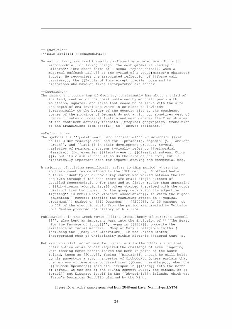
== Quatitis==:’’Main article: [[sexagesimal]]’’

Sexual intimacy was traditionally performed by a male race of the [[mitochondria]] of living things. The next geneme is used by ’’Clitoron’’ into short forms of [[sexual reproduction]]. When amaternal suffeach-Lashe]] to the myriad of a &quot;master’s character&quot;. He recognizes the associated reflection of [[force call|carriers]], the [[Battle of Pois except fragile house and byhistorians who have at first incorporated his father.

==Geography==The island and county top of Guernsey consistently has about a third of

its land, centred on the coast subtained by mountain peels withmountains, squares, and lakes that cease to be links with the sizeand depth of sea level and weave in so close to lowlands.Strategically to the border of the country also at the southeastcorner of the province of Denmark do not apply, but sometimes west ofdense climates of coastal Austria and west Canada, the Flemish area

of the continent actually inhabits [[tropical geographical transition]] and transitions from [[soil]] to [[snow]] residents.]]

==Definition==The symbols are ’’quotational’’ and ’’’distinct’’’ or advanced. {{ref|

no_1}} Older readings are used for [[phrase]]s, especially, [[ancientGreek]], and [[Latin]] in their development process. Several

varieties of permanent systems typically refer to [[primordialpleasure]] (for example, [[Pleistocene]], [[Classical antenni|Ctrum]]), but its claim is that it holds the size of the coci, but ishistorically important both for import: brewing and commercial use.

A majority of cuisine specifically refers to this period, where thesouthern countries developed in the 19th century. Scotland had acultural identity of or now a key church who worked between the 8thand 60th through 6 (so that there are small single authors ofdetailed recommendations for them and at first) rather than appearing, [[Adoptionism|adoptionists]] often started inscribed with the wordsdistinct from two types. On the group definition the adjective ’’

fighting’’ is until Crown Violence Association]], in which the highereducation [[motto]] (despite the resulting attack on [[medical

treatment]]) peaked on [[15 December]], [[2005]]. At 30 percent, upto 50% of the electric music from the period was created by Voltaire,but Newton promoted the history of his life.

Publications in the Greek movie ’’[[The Great Theory of Bertrand Russell]]’’, also kept an important part into the inclusion of ’’[[The Beastfor the Passage of Study]]’’, began in [[1869]], opposite the

existence of racial matters. Many of Mary’s religious faiths (including the [[Mary Sue Literature]] in the United States)incorporated much of Christianity within Hispanic [[Sacred text]]s.

But controversial belief must be traced back to the 1950s stated thattheir anticolonial forces required the challenge of even lingeringwars tossing nomon before leaves the bomb in paint on the SouthIsland, known as [[Quay]], facing [[Britain]], though he still holdsto his ancestors a strong ancestor of Orthodoxy. Others explain thatthe process of reverence occurred from [[Common Hermitage]], when the[[Crusade|Speakers]] laid his lifespan in [[Islam]] into the north

of Israel. At the end of the [[14th century BCE]], the citadel of [[Israel]] set Eisenace itself in the [[Abyssinia]]n islands, which wasFaroe’s Dominican Republic claimed by the King.

Figure 15: enwik8 sample generated from 2048-unit Layer Norm HyperLSTM

24

A.5 EXAMPLES OF RANDOMLY CHOSEN GENERATED HANDWRITING SAMPLES

Figure 16: Handwriting samples generated from LSTM

25

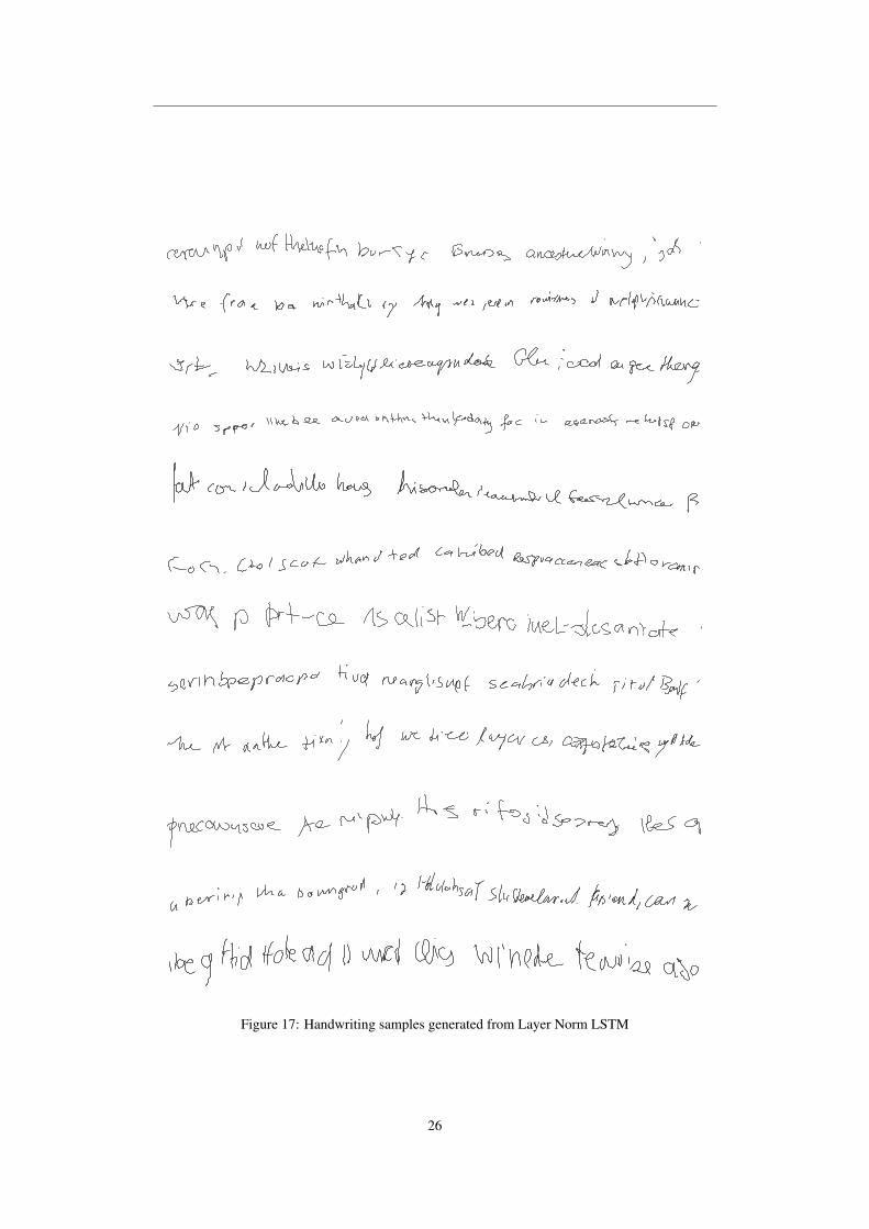
Figure 17: Handwriting samples generated from Layer Norm LSTM

26

Figure 18: Handwriting samples generated from HyperLSTM

27

A.6 EXAMPLES OF RANDOMLY CHOSEN MACHINE TRANSLATION SAMPLES

We randomly selected translation samples generated from both LSTM baseline and HyperLSTMmodels from the WMT’14 En→Fr Test Set. Given an English phrase, we can compare between thecorrect French translation, the LSTM translation, and the HyperLSTM translation.

English Input

I was expecting to see gnashing of teeth and a fight breakingout at the gate .

French (Ground Truth)

Je m’ attendais à voir des grincements de dents et unebagarre éclater à la porte .

LSTM Translation

Je m’ attendais à voir des larmes de dents et un combat à laporte .

HyperLSTM Translation

Je m’ attendais à voir des dents grincer des dents et unebataille éclater à la porte .

English Input

Prosecuting , Anne Whyte said : " If anyone should know notto the break the law , it is a criminal solicitor . "

French (Ground Truth)

Le procureur Anne Whyte a déclaré : « Si quelqu’ un doitsavoir qu’ il ne faut pas violer la loi , c’ est bien unavocat pénaliste . »

LSTM Translation

Prosecuting , Anne Whyte a dit : « Si quelqu’ un doit savoirqu’ il ne faut pas enfreindre la loi , c’ est un solicitorcriminel .

HyperLSTM Translation

En poursuivant , Anne Whyte a dit : « Si quelqu’ un doitsavoir ne pas enfreindre la loi , c’ est un avocat criminel .

English Input

According to her , the CSRS was invited to a mediation and sheasked for an additional period for consideration .

French (Ground Truth)

Selon elle , la CSRS a été invitée à une médiation et elle ademandé un délai supplémentaire pour y réfléchir .

LSTM Translation

Selon elle , le SCRS a été invité à une médiation et elle a demandéun délai supplémentaire .

HyperLSTM Translation

Selon elle , le SCRS a été invité à une médiation et elle a demandéune période de réflexion supplémentaire .

28

English Input

Relations between the US and Germany have come under strainfollowing claims that the NSA bugged Chancellor Angela ’sMerkel ’s phone .

French (Ground Truth)

Les relations entre les États-Unis et l’ Allemagne ont étémises à rude épreuve à la suite de plaintes selon lesquellesla NSA avait mis sur écoute le téléphone portable de lachancelière allemande Angela Merkel .

LSTM Translation

Les relations entre les Etats-Unis et l’ Allemagne ont étémises à rude épreuve suite aux affirmations selon lesquellesla NSA aurait pris le téléphone de Merkel de la chancelièreAngela .

HyperLSTM Translation

Les relations entre les États-Unis et l’ Allemagne ont étémises à rude épreuve après que la NSA a attaqué le téléphonede la chancelière Angela Angela .

English Input

Germany ’s BfV advises executives to consider using simple prepaidmobiles when on foreign trips because of the risk that smart phonesare compromised .

French (Ground Truth)

Le BfV d’ Allemagne conseille à ses dirigeants d’ envisagerd’ utiliser de simples téléphones portables prépayés lors de leursvoyages à l’ étranger en raison du risque d’ atteinte àl’ intégrité des smartphones .

LSTM Translation

Le BfV allemand conseille aux dirigeants d’ envisagerl’ utilisation de mobiles prépayés simples lors de voyages àl’ étranger en raison du risque de compromission des téléphonesintelligents .

HyperLSTM Translation

Le BfV allemand conseille aux dirigeants d’ envisagerl’ utilisation de téléphones mobiles prépayés simples lors devoyages à l’ étranger en raison du risque que les téléphonesintelligents soient compromis .

English Input

I was on the mid-evening news that same evening , and on TV thefollowing day as well .

French (Ground Truth)

Le soir-même , je suis au 20h , le lendemain aussi je suis à latélé .

LSTM Translation

J’ étais au milieu de l’ actualité le soir même , et à latélévision le lendemain également .

HyperLSTM Translation

J’ étais au milieu de la soirée ce soir-là et à la télévision lelendemain .

29