13-5-2010

Guocheng Zhu

zgc945ahhn@163.com

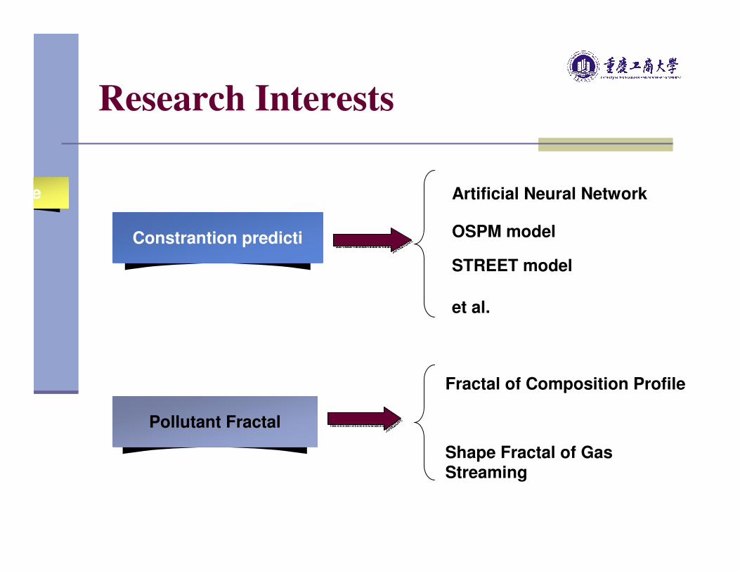
Research Interests

Artificial Neural Network

OSPM model

STREET model

et al.

Fractal of Composition Profile

Shape Fractal of Gas Streaming

Pollutant Fractal

Constrantion predicti

Text in here

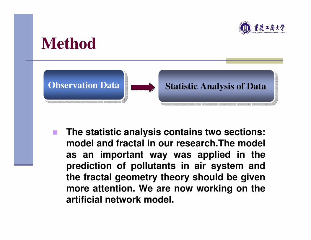
Method

� The statistic analysis contains two sections: model and fractal in our research.The model as an important way was applied in the prediction of pollutants in air system and the fractal geometry theory should be given more attention. We are now working on the artificial network model.

Observation DataObservation Data Statistic Analysis of DataStatistic Analysis of Data

21 3

4

Area of Coverage

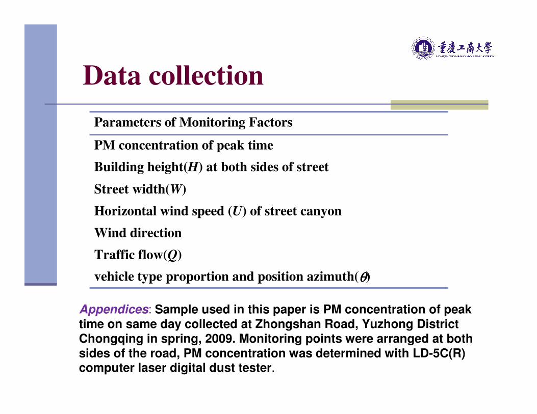
Data collection

Parameters of Monitoring Factors

PM concentration of peak time

Building height(H) at both sides of street

Street width(W)

Horizontal wind speed (U) of street canyon

Wind direction

Traffic flow(Q)

vehicle type proportion and position azimuth(θθθθ)

Appendices: Sample used in this paper is PM concentration of peak time on same day collected at Zhongshan Road, Yuzhong District

Chongqing in spring, 2009. Monitoring points were arranged at both sides of the road, PM concentration was determined with LD-5C(R) computer laser digital dust tester.

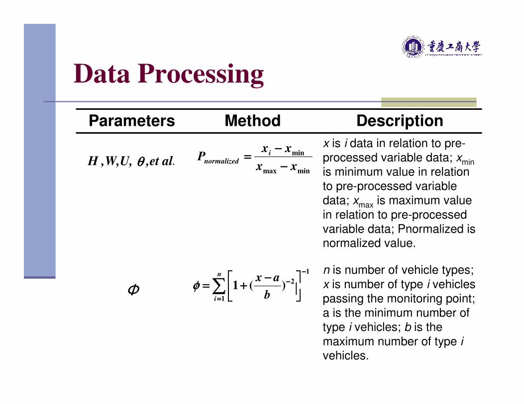
Data Processing

Parameters Method Description

H ,W,U, θθθθ ,et al.

x is i data in relation to pre-

processed variable data; xmin

is minimum value in relation

to pre-processed variable

data; xmax is maximum value

in relation to pre-processed

variable data; Pnormalized is normalized value.

Фn is number of vehicle types;

x is number of type i vehicles

passing the monitoring point;

a is the minimum number of

type i vehicles; b is the

maximum number of type ivehicles.

minmax

min

xx

xxP i

normalized−−−−

−−−−====

1

1

2)(1

−−−−

====

−−−−∑∑∑∑

−−−−++++====

n

i b

axφφφφ

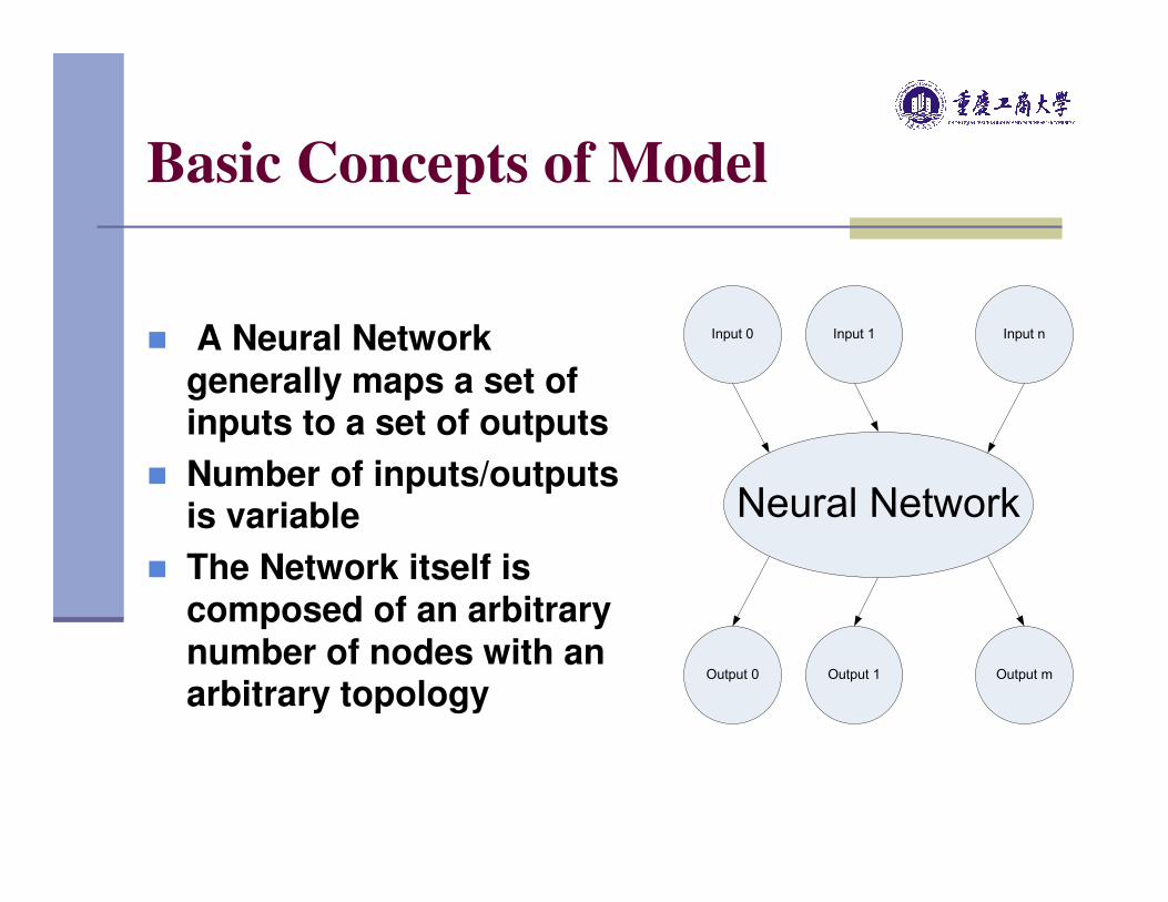
Basic Concepts of Model

Neural Network

Input 0 Input 1 Input n...

Output 0 Output 1 Output m...

� A Neural Network generally maps a set of inputs to a set of outputs

� Number of inputs/outputs is variable

� The Network itself is composed of an arbitrary number of nodes with an arbitrary topology

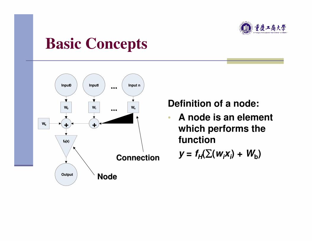
Basic Concepts

Definition of a node:

• A node is an element which performs the function

y = fH(∑∑∑∑(wixi) + Wb)

NodeNode

ConnectionConnection

ffHH((xx))

Input Input 00 Input Input 11 Input nInput n......

WW00 WW11 WWnn

++

OutputOutput

++

......

WWbb

Simulation Method of RBF Network

� Prediction effect of RBF network model is affected by the maximum nerve cells and network distribution density of radial basis function.

� To find two data of maximum nerve cells and network distribution density of radial basis function, simulation test under different conditions is required.

� Data range of test conditions is : maximum nerve cell is 1 to 20; interval 1; network density 0.1 to 2, interval 0.1.

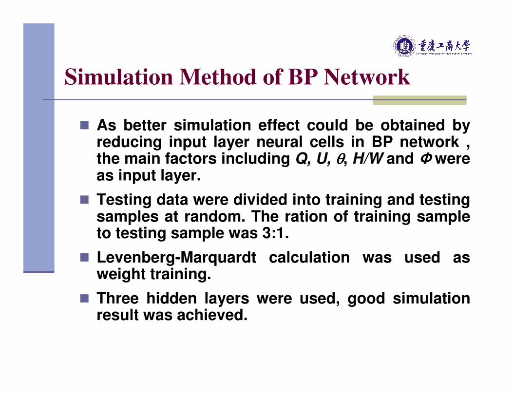
Simulation Method of BP Network

� As better simulation effect could be obtained by reducing input layer neural cells in BP network , the main factors including Q, U, θθθθ, H/W and ФФФФ were as input layer.

� Testing data were divided into training and testing samples at random. The ration of training sample to testing sample was 3:1.

� Levenberg-Marquardt calculation was used as weight training.

� Three hidden layers were used, good simulation result was achieved.

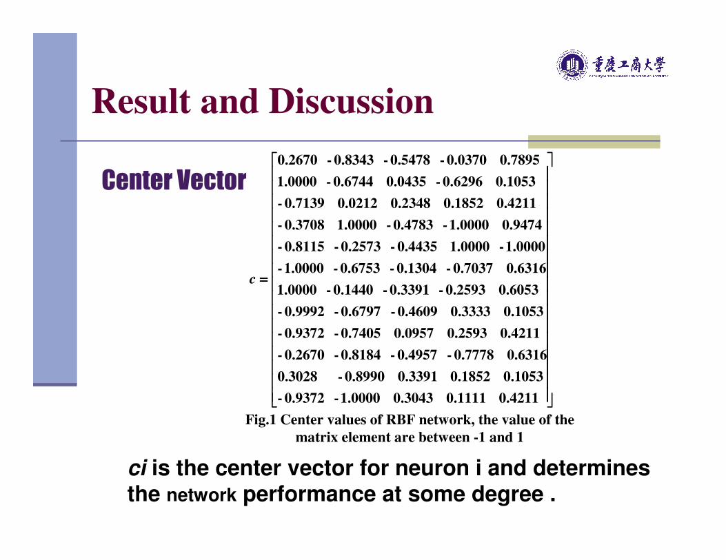
ci is the center vector for neuron i and determines the network performance at some degree .

Center Vector

Result and Discussion

====

0.4211 0.1111 0.3043 1.0000- 0.9372-

0.1053 0.1852 0.3391 0.8990- 0.3028

0.6316 0.7778- 0.4957- 0.8184- 0.2670-

0.4211 0.2593 0.0957 0.7405- 0.9372-

0.1053 0.3333 0.4609- 0.6797- 0.9992-

0.6053 0.2593- 0.3391- 0.1440- 1.0000

0.6316 0.7037- 0.1304- 0.6753- 1.0000-

1.0000- 1.0000 0.4435- 0.2573- 0.8115-

0.9474 1.0000- 0.4783- 1.0000 0.3708-

0.4211 0.1852 0.2348 0.0212 0.7139-

0.1053 0.6296- 0.0435 0.6744- 1.0000

0.7895 0.0370- 0.5478- 0.8343- 0.2670

c

Fig.1 Center values of RBF network, the value of the

matrix element are between -1 and 1

Aactivation function

∑=

==m

i

iikk pkXRy1

,2,1)(ˆ Lω

� Gaussian basis function was set as the activation

function of hidden layer in the RBF neural network.

The input vector was defined as X=(x1,x2,…xj,…,xn)

and the actual output Y=(y1,y2,…yk,…,yp). The non-

linear activation function allows for non-linear mapping of the input space to the network output. The

non-linear mapping for input layer is X →→→→ Ri (x )and the output layer R i (x) →→→→ｙｙｙｙｋｋｋｋ. The output layer value

for neuron k is given by

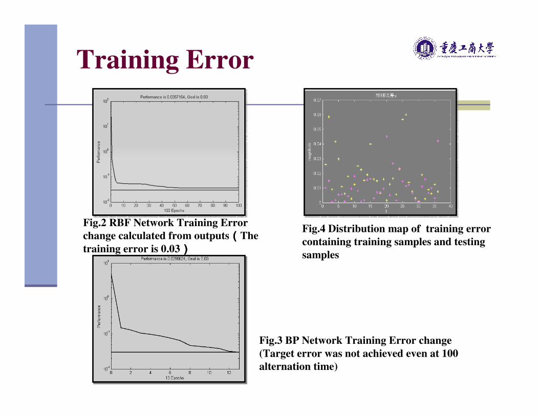
Training Error

Fig.2 RBF Network Training Error

change calculated from outputs（（（（The

training error is 0.03））））

Fig.3 BP Network Training Error change

(Target error was not achieved even at 100

alternation time)

Fig.4 Distribution map of training error

containing training samples and testing

samples

Distribution of Correlation Coefficient

Correlation

coefficient

Training

samples

Testing

samples

Greater than or

equal to 0.9 61.25% 18.5%

Between 0.8 and 0.9 31.5% 59.25%

Between 0.7 and 0.8 7.25% 22.25%

0.60.8

1.0

1.2

1.4

1.6

0.86

0.88

0.90

0.92

0.94

0.96

02

46

810

1214

1618

2022

Corr

elat

ion

co

effi

cien

t(

>=0.9)

maxim

um nerv

e cell num

ber

distribution density

Fig.5 Distribution map of correlation coefficient(≧≧≧≧0.9)

The maximum nerve cell number is 13 and the distribution density of radial basis function is 0.9, the simulation result of PM2.5 is best.

Comparison of Measured PM

and Calculated PM

0 5 10 15 20 250.150.200.250.300.350.400.45

0 2 4 6 8 10 12 14 16 18 20 22 24 26

0.15

0.20

0.25

0.30

0.35

0.40

0 2 4 6 8 10 12 14 16 18 20 22 24 26

0.150.200.250.300.350.400.45

dat

a o

f P

M2

.5 (

mg/m

3 )

sampl esdat

a o

f P

M5

(m

g/m

3 )

sampl es t es t i ng dat a s i mul at i ng dat a

t est i ng dat a s i mul at i ng dat a

d

ata

of

PM

10

(m

g/m

3 )

sampl es t es t i ng dat a s i mul at i ng dat a

Fig.6 Prediction result of PM based on RBF

0 5 10 15 20 250. 100. 150. 200. 250. 300. 350. 400. 45

sim

ula

tin

g d

ata

(mg/m

3 )

s ampl es t es t i ng dat a s i mul at i ng dat a of BP s i mul at i ng dat a of RBF

Fig.7 Comparison between prediction

results of PM2.5

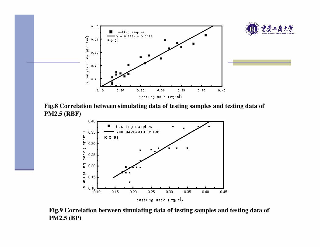
Fig.8 Correlation between simulating data of testing samples and testing data of

PM2.5 (RBF)

0. 15 0. 20 0. 25 0. 30 0. 35 0. 40 0. 450. 200. 250. 300. 350. 40simulating data(mg/m3 )

t es t i ng dat a ( mg/ m3)

t es t i ng s ampl es Y = 0 . 833X + 0 . 0428R=0. 94

Fig.9 Correlation between simulating data of testing samples and testing data of

PM2.5 (BP)

0.10 0.15 0.20 0.25 0.30 0.35 0.40 0.450.10

0.15

0.20

0.25

0.30

0.35

0.40 t es t i ng s ampl es Y=0. 94204X+0. 01196R=0. 91simulating data（mg/m3 ）

t es t i ng dat d ( mg/ m3)

Conclusions

� Prediction results of PM of different sizes are different, the simulating data of PM2.5 using RBF networks are better than those of PM5 and PM10.

� The simulation effect of RBF neural network is related to maximum nerve cell

number of network and the distribution density of radial basis function.When

the maximum nerve cell number is 13 and the distribution density of radial basis function is 0.9, the simulation result of PM2.5 is best.

� Using three hidden layers and Levenberg-Marquardt calculation method of BP neural network, good simulation effect could be achieved.

� For PM2.5, the correlation coefficient between simulating data of testing

sample and testing data of PM2.5 are 0.94 and 0.91, the ratio of training error

and testing error are 0.75 and 1.59 each by RBF and BP neural network. All

above show that PM2.5 of main traffic route come mainly from vehicle

emission. The two neural network established herein can be used to predict pollution of PM2.5 of main traffic route.

References

[1] Raga, G.B.; Moyne, L.L. E. Atmos Environ. 1996, 30(23): 3987-3993.

[2] Bai, X.P.; Zhang, Q.M.; Fang, D.; et al. Science & Technology Review. 2007,25(3): 45-49.(in Chinese)

[3] Gertler, A.W.; Gillies, J.A.; Pierson, W.R. Water, Air & Soil Pollution. 2000,123(1-4): 203-214.

[4] Hu, S.X.; Jiao, L.C. Introduction to Artificial Nerve Cell Calculation;Science Publishing House: Beijing, 1994. (in Chinese)

[5] Shen, Q.; Hu, D.W.; Shi, C. Applied Technology of Neural Network;Publishing House of Defense Technology University: Changsha. 1995. (in Chinese)

[6] Zhou, K. L.; Kang, Y.H. Neural Network Model and its MATLAB Simulation Program Design; Pubilshing House of Tsing HuaUniversity: Beijing, 2005. (in Chinese)

Thanks