guidelines for the annual and periodical compilation and ... documents/plc-6... · web...
TRANSCRIPT

Guidelines for the annual and periodical compilation and reporting of waterborne pollution inputs to the Baltic Sea
(PLC-water)
Table of Content
sGuidelines for the annual and periodical compilation and reporting of waterborne pollution inputs to the Baltic Sea (PLC-water).......................................................................................................................................1
1. Introduction.................................................................................................................................4
1.1. Aim of PLC assessments....................................................................................................................4
1.2. Aims of the PLC guidelines................................................................................................................5
1.3. PLC data reporting requirements......................................................................................................6
2. Framework and approach of waterborne pollution load compilation.........................................9
2.1. Overall framework............................................................................................................................9
2.2. Quantification of total inputs to the Baltic Sea.................................................................................9
2.3. Quantifying sources of waterborne nutrient inputs to the Baltic Sea.............................................10
2.4. Supporting tools.............................................................................................................................13
2.5. Basic definitions..............................................................................................................................13
2.6. Division of the Baltic Sea catchment area.......................................................................................15
3. Guidance on monitoring............................................................................................................20
3.1. Flow measurements.......................................................................................................................20
3.1.1. Riverine flow measurements..................................................................................................20
3.1.2. Wastewater flow measurements............................................................................................20
3.2. Sampling strategy for water samples: site selection and sampling frequency................................21
3.2.1. Riverine water sampling.........................................................................................................21
3.2.2. Wastewater sampling.............................................................................................................21
4. Quantification of load from monitored rivers............................................................................23
4.1. Methods for calculation of the load from monitored rivers...........................................................23
4.2. Methods for estimating the water flow for rivers where chemical and hydrological stations are not located at the same place....................................................................................................................24
5. Quantification of load from point sources.................................................................................26
5.1. Municipal Wastewater Treatment Plants (MWWTP)......................................................................26
5.2. Industrial plants (INDUSTRY)..........................................................................................................28
5.3. Aquaculture....................................................................................................................................28
6. Quantifying diffuse losses of nutrients.......................................................................................34
1

6.1. Quantification of the natural background nutrient losses..............................................................34
6.2. Quantification of nutrient losses from diffuse anthropogenic sources...........................................35
6.2.1. Documentation on used estimation methods for diffuse sources..........................................36
7. Methods for estimation of inputs from unmonitored areas......................................................38
8. Transboundary rivers.................................................................................................................39
8.1. Introduction....................................................................................................................................39
8.2. Definitions......................................................................................................................................39
8.3. Estimates of actual and net transboundary inputs used in the 2013 Copenhagen HELCOM Ministerial Declaration...............................................................................................................................41
8.4. Necessary information for quantifying transboundary input..........................................................42
8.5. Overview of transboundary rivers to take into account in annual reporting..................................42
9. Quantification of nutrient retention..........................................................................................50
9.1. Introduction....................................................................................................................................50
9.2. Quantification.................................................................................................................................50
9.3. Available retention data.................................................................................................................51
10. Quantification of sources of waterborne inputs to inland waters and to the sea......................53
10.1. Source oriented approach: Quantification of sources of waterborne inputs into inland surface waters 53
10.2. Load oriented approach: Quantification on sources of waterborne inputs to the sea...................53
10.2.1. Calculation principles for riverine load apportionment..........................................................54
11. Statistical methods and data validation.....................................................................................55
11.1. Introduction....................................................................................................................................55
11.2. Data gaps........................................................................................................................................55
11.3. Outliers...........................................................................................................................................56
11.4. Uncertainty of inputs (yearly input from a specific country or area)..............................................56
11.5. Hydrological normalization of riverine inputs.................................................................................58
11.6. Trend analysis and the estimation of change.................................................................................60
11.7. Testing fulfilment of BSAP reduction targets..................................................................................61
11.7.1. Testing without significant trends...........................................................................................61
11.7.2. Testing with significant trends................................................................................................62
11.8. Mathematical description of the Mann-Kendall trend test............................................................63
12. Quality assurance on water chemical analysis...........................................................................67
12.1. Specific aspects of quality assurance..............................................................................................67
12.2. Minimum quality assurance by the Contracting Parties.................................................................68
12.3. Inter-laboratory comparison tests on chemical analyses...............................................................68
12.4. The PLC-6 inter-laboratory comparison test on chemical analyses................................................69
2

12.5. Validation of PLC-Water chemical data..........................................................................................69
12.6. Recommended limits of quantification (LOQ).................................................................................70
12.7. Values under the limit of quantification.........................................................................................71
12.8. Technical notes on the determination of variables in rivers and wastewater................................71
13. Annual PLC reporting requirements...........................................................................................75
13.1. Reporting of the inputs from monitored rivers...............................................................................75
13.2. Reporting of the input from unmonitored areas............................................................................76
13.3. Reporting of the inputs from direct point sources..........................................................................76
13.4. Reporting on quality assurance......................................................................................................77
13.5. Reporting on uncertainty on national data sets..............................................................................77
14. Periodic PLC reporting requirements.........................................................................................78
14.1. Source-orientated approach: Methodology for quantifying sources of waterborne inputs to inland waters 78
14.1.1. Data requirements..................................................................................................................78
14.1.2. Point source discharges into inland surface waters and direct discharges from point sources79
14.1.3. Diffuse losses to inland surface waters...................................................................................83
14.1.4. Natural background losses into inland surface waters...........................................................83
14.1.5. Transboundary inputs.............................................................................................................84
14.1.6. Retention of nutrients............................................................................................................84
14.2. Load-oriented approach - reporting riverine load apportionment.................................................85
14.3. Reporting on uncertainty on national data sets..............................................................................86
15. References.................................................................................................................................87
Annex 1. List of definitions and acronyms.................................................................................................92
Annex 2. Annual reporting formats...........................................................................................................95
Annex 3. Periodic reporting formats.........................................................................................................96
Annex 4. Example of instructions to personnel carrying out the sampling...............................................97
Annex 5. Examples on measurement uncertainty estimations.................................................................99
Annex 6. Examples on reporting industrial point sources with references to IE Directive and PRTR Regulation 101
Annex 7. EMEP assessment of atmospheric nitrogen and heavy metal deposition on the Baltic Sea.....105
Annex 8. List of HELCOM PLC Contacts...................................................................................................109
3

1. Introduction
Since the establishment of the Convention for the Protection of the Marine Environment of the Baltic Sea Area (Helsinki Convention) in 1974, the Commission for the Protection of the Marine Environment of the Baltic Sea Area (Helsinki Commission or HELCOM for short) has been working to reduce the inputs of nutrients to the sea. Through coordinated monitoring, HELCOM has, since the mid-1980s been compiling information about the magnitude and sources of nutrient inputs into the Baltic Sea. By regularly compiling and reporting data on pollution inputs, HELCOM is able to follow the progress towards reaching politically agreed nutrient reduction input goals.
In 2007, the HELCOM Baltic Sea Action Plan (BSAP) was adopted by the Baltic Sea coastal countries and the European Community (HELCOM 2007). The BSAP has the overall objective of reaching good environmental status in the Baltic Sea by 2021, by addressing eutrophication, hazardous substances, biodiversity and maritime activities. The BSAP included for the first time ever a nutrient reduction scheme based on maximum allowable inputs (MAI) of nutrients to achieve good status in terms of eutrophication derived through modelled calculations by the Baltic Nest Institute (BNI) – Sweden. The plan also adopted provisional country-wise allocation of reduction targets (CARTs) to fulfil MAI through which the responsibility to reach these nutrient reductions targets is shared according to the polluter pays principle.
The 2013 HELCOM Copenhagen Ministerial Declaration (HELCOM 2013) agreed on revised MAI and new CARTs that were calculated based on improved eutrophication targets and models, more complete data on nutrient inputs (the one produced by the PLC-5.5 project) and revised allocation principles.
The present document contains guidelines prepared as part of the project Sixth Baltic Sea Pollution Load Compilation (PLC-6) and should serve to guide the Contracting Parties of the Helsinki Commission in their national monitoring and reporting of pollution inputs in order to allow for compilation of harmonized data for producing region-wide PLC assessments, and providing data for the follow up of MAI and CARTs. The guidelines are in line with EU quality assurance standards and OSPAR methodologies.
Although the PLC-6 assessment will cover total inputs to the Baltic Sea, including inputs to the sea via the atmosphere, these guidelines focus on compilation of waterborne input data (atmospheric deposition within the Baltic Sea catchment area is included in the source apportionment of loads to inland surface waters). Atmospheric deposition of nitrogen, cadmium, lead and mercury to the Baltic Sea is assessed and reported annually by EMEP (Co-operative Programme for Monitoring and Evaluation of Long-Range Transmission of Air Pollutants in Europe) to HELCOM.
A detailed description of the contents of these guidelines is given in Chapter 2.
1.1. Aim of PLC assessmentsFor developing reliable, useful and easily elaborated PLC assessments and for evaluating progress in fulfilling MAI and CART, it is very important to establish a consistent, harmonized, comparable, quality assured data series without data gaps etc. This calls for the use of harmonized and comparable methodology, and for reporting of well quality assured data to the PLC-database.
The PLC assessments aim to follow up on the implementation of the Convention on the Protection of the Marine Environment of the Baltic Sea Area (Helsinki Convention) by its Contracting Parties, in particular paragraphs 1 and 2 under Article 6 of the Convention:
The Contracting Parties undertake to prevent and eliminate pollution of the Baltic Sea Area from land-based sources by using, inter alia, Best Environmental Practice
4

for all sources and Best Available Technology for point sources. The relevant measures to this end shall be taken by each Contracting Party in the catchment area of the Baltic Sea without prejudice to its sovereignty.
The Contracting Parties shall implement the procedures and measures set out in Annex III. To this end they shall, inter alia, as appropriate co-operate in the development and adoption of specific programmes, guidelines, standards or regulations concerning emissions and inputs to water and air, environmental quality, and products containing harmful substances and materials and the use thereof.
The PLC assessments also support follow-up of the implementation of the 2007 HELCOM Baltic Sea Action Plan (BSAP) (HELCOM 2007), which includes a nutrient reduction scheme based on maximum allowable inputs (MAI) and country-wise allocation of reduction targets (CARTs), and the updated MAI and new CARTs decided on the 2013 HELCOM Copenhagen Declaration (HELCOM 2013).
In implementing the objectives of the Convention and the BSAP nutrient reduction scheme, the Helsinki Commission (HELCOM) needs reliable data on inputs to the Baltic Sea from land-based sources in order to:
Assess the effectiveness of measures taken to abate the pollution in the Baltic Sea catchment area Follow-up on progress towards MAIs and CARTs, and Be able to identify further cost-effective measures for reducing pollution.
Such data also supports assessments of the state of the open sea and coastal waters.
The objectives of periodic waterborne pollution input compilations (PLC-Water) regarding pollution of the Baltic Sea from land-based sources are to:
Compile information on the waterborne inputs via rivers and direct discharges of important pollutants entering the Baltic Sea from different sources in the Baltic Sea catchment area on the basis of harmonized monitoring and modelling methods
Follow-up the long-term changes in the pollution input from various sources by normalizing data and making trend analysis with standardized methodologies
Identify the main sources of pollution to the Baltic Sea in order to support prioritization of measures
Assess overall the effectiveness of measures taken to reduce the pollution inputs into the Baltic Sea catchment area
Assess the development of waterborne and airborne nutrient inputs from different countries to the different Baltic Sea sub-basins in order to evaluate progress in fulfilling nutrient reduction targets of the Baltic Sea Action Plan
Provide pollution input information for assessment of long-term changes and the state of the marine environment in the open sea and the coastal zones.
1.2. Aims of the PLC guidelinesThe aims of these guidelines are to:
Provide a framework and serve as a tool for HELCOM Contracting Parties in national monitoring, quantification and reporting on total waterborne inputs of nitrogen, phosphorus and selected heavy metals and their sources to the Baltic Sea to obtain a harmonized and comparable dataset covering the whole Baltic Sea region
5
Enhance the comparability, consistency and quality of the PLC data and, to the extent possible ensure harmonized practises between Contracting Parties when carrying out PLCs and when assessing PLC data for source quantification
Provide guidance in cases where there is a choice of methods Ensure transparency, so that any differences in methods are easy to detect. This concerns cases
where harmonization of practices cannot be obtained due to climatic, topographical, hydrological or other differences between Contracting Parties.
To fulfil the evolving data requirements of HELCOM and its Contracting Parties, these guidelines should be regularly evaluated and updated by experts and adopted by the responsible subsidiary body of HELCOM.
1.3. PLC data reporting requirementsThe PLC monitoring and reporting requirements reflect the data needs of HELCOM for supporting the implementation of the Helsinki Convention and the Baltic Sea Action Plan (HELCOM 2007 and HELCOM 2013), while bearing in mind also the monitoring and reporting needs of those HELCOM Contracting Parties that are also EU Member States.
According to HELCOM Recommendation 26/2, waterborne pollution load compilation (PLC-Water) data is to be reported by Contracting Parties to the Commission both on an annual and periodical basis:
Annually, total inputs of nutrients and hazardous substances to the sea should be reported by quantifying inputs from monitored rivers, unmonitored areas, and point sources discharging directly to the sea (Table 1.1).
Periodically (every six years), comprehensive waterborne pollution load compilations should be carried out to quantify, in addition to the total inputs to the sea (annual reporting), also waterborne discharges from point sources, losses from diffuse sources as well as natural background losses into inland surface waters within the Baltic Sea catchment area located within the borders of the Contracting Parties (Table 1.1 and 1.2).
The parameters to be reported have been agreed upon by the Contracting Parties as either obligatory or voluntary (Tables 1.1 and 1.2). Further, the limits of quantification/detection for the different parameters are taken into account when evaluating if they must be reported. See the List of definitions in Annex 1 for explanations of the terms measured, calculated and estimated.
Table 1.1 lists the annual reporting obligation and Table 1.2 the additional reporting requirement besides the annual reporting during the periodic assessment every six years.
The annual reporting requirements are further specified in Chapter 13 and more details on the additional reporting requirements for the periodical reporting requirements are given in Chapter 14. The specific annual reporting formats are included in Annex 2 and the periodical reporting formats in Annex 3.
6

Table 1.1. Variables to be reported within PLC-Water (annually).
Parameters Point sources discharging directly to the Baltic Sea7
Monitored rivers*
Unmonitoredareas5
Transboundary at the border of the
Contracting Party10
Municipal Effluents*
Industrial Effluents*
Aqua-culture*
BOD53
TOC+ +9 + v
v v v
Ptotal
PPO4
Ntotal
NNH4
NNO24
NNO34
++8
++vv
+v+vvv
+
+
++++++
++++++
+
+
HgCdZnCuPbNiCr
+2
+2
+2
+2
+2
+2
+2
+9
+9
+9
+9
+9
+9
+9
+1
+1
vv+1
vv
+1
+1
vv+1
vv
vvvvvvv
Flow + + +6 + + +
Footnotes:
+ obligatoryv voluntary1 Except for rivers where heavy metal concentrations are below the limit of quantification. If all measurements are
below LOQ, then the value should be reported as zero and information provided about number of samples below the LOQ. (Those countries who do not use LOQ should replace it with LOD.)
2 Heavy metals are obligatory for municipal WWTPs larger than 20,000 PE. 3 If BOD7 is measured, it will be stored in the HELCOM PLC-Water database, and for PLC assessments a
conversion factor BOD5 = BOD7 /1.15 will be used for converting to BOD54 Can be monitored and reported as the sum of oxidized nitrogen (NO2,3-N).5 Diffuse sources entering directly to the sea include inputs from scattered dwellings and rainwater overflows.6 For aquaculture where it is relevant (outlet for discharges).7 Point sources discharging directly to the Baltic Sea should preferably be reported individually, but can be reported
as a sum for every Baltic Sea sub-catchment for municipal effluents, industrial effluents, and aquaculture, respectively.
8 Should be measured or calculated9 If monitoring of the parameter is required in the permit conditions of the industrial plant10 Surface water retention of TN and TP on transboundary inputs in the receiving catchment should be reported if
updated data/information is available compared to former reported/used data.* In those cases where less than 50% of the recorded concentrations are below the limit of quantification, the
estimated concentration should be calculated using the equation: Estimate = ((100%-A) x LOQ)/100 where A= percentage of samples below LOQ (cf. Chapter 12.7). This is according to one of the options listed in the guidance document on monitoring adopted by EU under the IE Directive. (Those countries who do not use LOQ should replace it with LOD in the equation.)
7

Table 1.2. In addition to the annual reporting in Table 1.1, the following data and information are also to be reported periodically for PLC-Water every sixth year.
Parameters Monitored areas Unmonitored areas
Point sources1
Diffuse sources2
Natural background
Point sources3
Diffuse sources2
Natural back-ground losses
Retention (monitored and unmonitored, respectively)4
Ptotal
Ntotal
HgCdPb
++vvv
++
++
++vvv
++
++
++
Flow + +
Footnotes:
+ obligatoryv voluntary1 Reported for MWWTP, industries and aquaculture separately2 Nutrient losses from diffuse sources can be estimated either as the total for all sources or as losses divided by
individual source/pathways 3 The point sources from unmonitored areas are to be reported individually although they can be aggregated
separately for MWWTP, industries and aquaculture (in monitored areas point sources are to be reported individually).
4 Preferably a separate retention value should be estimated for each pathway, otherwise a single value can be provided. See chapter 9 for calculation of retention.
Within the PLC-6 project, a questionnaire has been circulated to Contracting Parties, requesting information on parameters being monitored, and the frequency of monitoring, in rivers and point sources. The results of the questionnaire have been compiled and are available on the PLC-6 project webpage on the HELCOM website.
8

2. Framework and approach of waterborne pollution load compilation
2.1. Overall frameworkThe guidelines focus mainly on nutrients but also cover quantification of total waterborne inputs of cadmium, lead and mercury).
The overall structure of the guidelines is shown in Figure 2.1, reflecting the general framework and approach used for quantifying total waterborne inputs to the Baltic Sea and for quantifying importance of different nutrient sources. The different topics are described in separate chapters with cross-reference to other chapters to avoid repetition of information. The reporting requirements are assigned to separate chapters on annual obligations (Chapter 13) and on periodical reporting (Chapter 14), respectively. The details related to reporting sheets can be found in Annex 2 and 3.
Figure 2.1. Structure of the pollution load compilation (PLC) guidelines illustrating where different topics are scrutinized.
The main definitions and abbreviations used in the guidelines are listed in Annex 1.
Retention is indicated in a grey box as it is used for quantifying transboundary inputs entering the Baltic Sea, quantification of sources entering into freshwater and for source apportionment.
2.2. Quantification of total inputs to the Baltic SeaContracting Parties are obliged annually to quantify and report total waterborne inputs from point and diffuse sources entering to the Baltic Sea from their catchment (HELCOM Recommendation 26/2: Compilation of Waterborne Pollution Load (PLC-Water)) (HELCOM 2005). Transboundary waterborne nutrient inputs reaching the Baltic Sea should be included in the total waterborne inputs, and the transboundary part of Contracting Parties waterborne inputs should be quantified to allow for the follow
9

up on the progress towards reaching the country-wise allocation of reduction targets (CARTs) under the nutrient reductions scheme adopted in the 2013 HELCOM Copenhagen Ministerial Declaration (HELCOM 2013).
The total waterborne input is the sum of total riverine inputs from monitored and unmonitored areas plus the input from point sources discharging directly to the Baltic Sea (also called direct discharges) and is quantified for nutrients and selected heavy metals per Contracting Party and per Baltic Sea sub-basin as:
TIx = ∑Ix monitored rivers + ∑Ix unmonitored areas + ∑Ix point sources discharging directly to the sea (2.1)
where
TIx is total waterborne inputs (I) of the substance x from a country.
The objective is to provide estimates that are as exact as possible, of the total waterborne inputs entering the Baltic Sea sub-basins including estimates of the share of transboundary waterborne nutrient inputs entering the Baltic Sea. Further, the objectives are to quantify total inputs of cadmium, lead and mercury. The annual reporting obligation is described in Chapter 13 and Annex 2.
2.3. Quantifying sources of waterborne nutrient inputs to the Baltic SeaContracting Parties are obliged to periodically (every six years) quantify and report nutrient discharges from point sources, and nutrient losses from natural and anthropogenic diffuse sources into inland surface waters within monitored and unmonitored catchment areas of the Baltic Sea located within their borders. Further the Contracting Parties are obliged to periodically quantify and report the sources of the total nutrient inputs entering the Baltic Sea taking into account the retention in inland surface waters. Quantification of sources of inputs is explained in chapters 5 and 6, and quantification of transboundary loads in Chapter 8.
Two source quantification approaches are described in Chapter 10:
Quantifying the total gross loads from point sources, diffuse sources and natural background losses into inland surface waters within the whole Baltic Sea catchment area is important to get a comprehensive overview of the total loading originating in the Baltic Sea catchment area and the nutrient sources behind these inputs. This is called the “source oriented approach”.
Quantifications of the sources of the total waterborne nutrient inputs to the sea are used for assessing the main sources of waterborne nutrient inputs to the sea, and to evaluate the resulting effects of land-based measures for reducing waterborne nutrient inputs (to the sea) taking into account the importance of inland surface water retention. This is called the “load oriented approach”.
The periodical reporting requirements are described in Chapter 14 and in Annex 3.
Examples of different point and diffuse sources and pathways for nutrients (and heavy metals) to inland surface waters and waterborne inputs to the sea are shown in Figure 2.2. The Contracting Parties are not obliged to quantify all the pathways, only the (major) point and diffuse sources described in chapters 5 and 6. Figure 2.3 illustrates how different sources add nutrients to inland surface waters and how retention in the waters of the catchment area removes and/or retains nutrients.
10

Figure 2.2. Sources and pathways of nutrients (and heavy metals) to the marine environment. Some of the arrows are only of relevance for one of the nutrients e.g. combustion and ammonia volatilization (nitrogen). For the atmospheric compartment, atmospheric deposition on surface inland waters is included in inputs from diffuse sources and only airborne inputs on inland surface waters are included in the PLC guidelines). (Airborne emissions and deposition to the sea are covered in EMEPs annual reports and fact sheets on airborne inputs, cf. Annex 7)
Retention is the removal of e.g. nutrients in surface waters of river systems including lakes, flooded riverbanks and wetlands caused by biological, chemical and physical processes (Figure 2.3). As a proportion of the nutrients entering inland surface water is retained or removed, retention must be taken into account when e.g. evaluating sources for total waterborne inputs to sea and quantifying net contribution of riverine transboundary inputs. Chapter 9 deals with retention in inland surface waters.
11
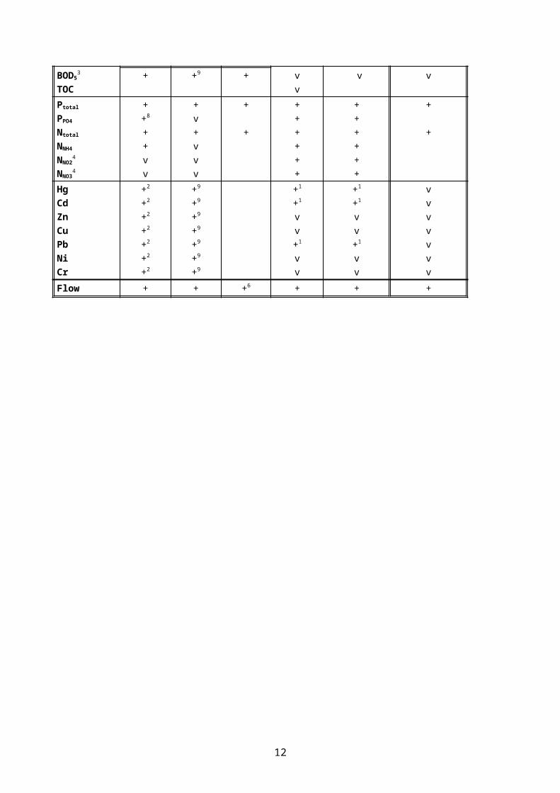
Figure 2.3. Illustration of inputs to and removal processes (retention) from a river system (inland surface waters), which includes transboundary inputs, monitored and unmonitored areas, and direct inputs to the sea. For definitions, see Figure 2.4 and Annex 1.
12

2.4. Supporting toolsThe guidelines also include chapters regarding:
An overview of the parameters to monitor (Chapter 1) Guidance on how to take and handle water samples in rivers, and to monitor river flow and
discharge from some point sources (Chapter 3) Statistical methods for assessing PLC data (estimating uncertainty, normalization, trend analysis
etc.) and how to handle data gaps and outliers (Chapter 11) Minimum quality assurance expected by the Contracting Parties, inter-laboratory comparison test,
recommended limits of quantification (Chapter 12) List of definitions and acronyms, detailed instructions on reporting sheets, a short description of
used methodology to quantify atmospheric deposition in the Baltic Sea etc. (Annexes 1-9).
Some of the statistical methods included in the guidelines serve as guidance for elaborating PLC assessments. They will be performed in a uniform way within the HELCOM PLC data processing framework, and Contracting Parties are not required to make these calculations (further specifications are given in Chapter 11).
2.5. Basic definitionsFigure 2.4 illustrates the definitions of catchment areas, monitored areas, unmonitored areas, direct and indirect point sources and transboundary inputs (see also the list of definitions and acronyms contained in Annex 1). It should be noted that in some cases, the locations of hydrological and chemical monitoring stations differ from each other (see Chapter 4.2). In these cases, the chemical monitoring station defines the monitored catchment.
Direct point sources are municipal wastewater treatment plants, industrial plants and aquaculture plants discharging directly into the Baltic Sea. Further it includes marine aquaculture plants situated and discharging in marine waters.
A river that has its outlet to the Baltic Sea at the border between two countries is considered a border river. For these rivers, the inputs to the Baltic Sea are divided between the countries in relation to each country’s share of total load.
A transboundary river has its outlet to the sea situated in one country, but is receiving transboundary inputs from one or several upstream countries. Chapter 8 includes a list of the transboundary rivers where Contracting Parties should quantify the proportion of transboundary inputs. In some cases a river is both border and transboundary, as shown for Nemunas in Figure 8.1.
13

14

Figure 2.4. Illustration of some key definitions used in these guidelines – see also Annex 1 “List of definitions and acronyms”. (I=Industry, M=MWWTPs, A=aquaculture, I=Island, Hy=hydrographic monitoring station, Ch=Chemical monitoring stations, u=unmonitored, m=monitored, t=transbounday, d= direct inputs)
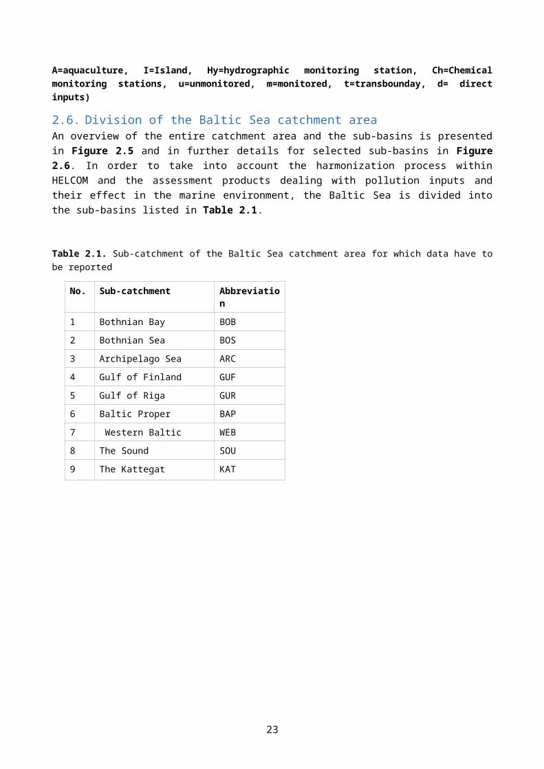
2.6. Division of the Baltic Sea catchment areaAn overview of the entire catchment area and the sub-basins is presented in Figure 2.5 and in further details for selected sub-basins in Figure 2.6. In order to take into account the harmonization process within HELCOM and the assessment products dealing with pollution inputs and their effect in the marine environment, the Baltic Sea is divided into the sub-basins listed in Table 2.1.
Table 2.1. Sub-catchment of the Baltic Sea catchment area for which data have to be reported
No. Sub-catchment Abbreviation
1 Bothnian Bay BOB
2 Bothnian Sea BOS
3 Archipelago Sea ARC
4 Gulf of Finland GUF
5 Gulf of Riga GUR
6 Baltic Proper BAP
7 Western Baltic WEB
8 The Sound SOU
9 The Kattegat KAT
15

To enable for assessments the input figures must be presented separately for each sub-catchment by each Contracting Party. A GIS shape file of the sub-basins can be downloaded via the HELCOM Map and Data Service.
16

Figure 2.5. The Baltic Sea catchment area and sub-basins as defined for PLC-Water.
Figure 2.6. Close-ups of the Baltic Sea catchment area and sub-basins divisions in the Danish straits, the Archipelago Sea and Gulf of Riga, and The Quark.
The main part of the catchment to the Baltic Sea is monitored and it is mainly minor rivers and catchment areas close to the sea (coastal areas) that are unmonitored (Figures 2.7 and 2.8).
17

Figure 2.7. Monitored and unmonitored areas in the HELCOM countries, transboundary catchments and parts of the catchment area outside the HELCOM countries.
18

Figure 2.8. Close up of Danish, German, western Poland and southern Swedish monitored and unmonitored areas in the HELCOM countries, transboundary catchments and parts of the catchment area outside the HELCOM countries.
19

3. Guidance on monitoringThis chapter gives guidance on how to monitor riverine and wastewater flow as well as how to take and handle water samples in rivers, municipal wastewater treatment plants and industrial plants.
3.1. Flow measurements 3.1.1.Riverine flow measurements For rivers with riverine water level and flow (velocity) measurements , the location of permanent hydrological stations (if any), measurement equipment, frequency of water level and flow measurement should at least follow the World Meteorological Organization (WMO) Guide to Hydrological Practices (WMO-No. 168, 2008) and national quality assurance (QA) standards. See also Chapter 3.1.2. on requirements of monitoring water flow.
The frequency of flow measurement should as a minimum correspond to the sampling frequency for the determination of the load and be carried out at least 12 times per year.
Preferable the discharge (or at least the water level) should be monitored continuously and close to where chemical samples are taken. If the discharges are not monitored continuously the measurements must cover low, mean and high river flow rates, i.e. they need not necessarily to be done at regular intervals, but should as a minimum reflect the main annual river flow pattern. A relation between discharge and water level should be established based on the regular discharge measurement in order to calculate daily flow in the river. Continuously controlled and regularly calibrated equipment (e.g. current meters) and carefully performed measurements together with an accurate calculation can diminish errors.
3.1.2.Wastewater flow measurementsThe accuracy of the wastewater flow measurements in municipal sewage systems and indus trial plants are in many cases of a considerable lower quality than can be expected. Measurement errors of more than 20% are not unusual. However, the accuracy can be improved by increasing the awareness of the types of errors, by elimination of these errors and by continuous maintenance of the measurement system and its accuracy. A relative error less than 5%, which can be achieved by most of the methods used in open and closed systems, should be the target in each case.
An open flow measurement system includes channels, flumes and weirs, e.g. Venturi- and Parshall channels/flumes and Thompson (V-notch) weirs. In closed systems the measurement takes place in pipes using different kind of flow meters, e.g. ultrasonic (Acoustic -Doppler) and electromagnetic meters. Most of these available methods are reliable if properly used and can be recommended for the wastewater flow measurement. In this chapter only some general instructions related to the flow measurement and improvement of its accuracy are presented. More detailed information can be obtained from numerous standards (e.g. ISO-/DIN-standards), guidelines and handbooks (e.g. WMO-No. 168, 2008) that deal with flow measurement methods, the theory and prerequisites of them, as well as possible sources of error, calibration methods etc.
A flow measurement system should be chosen so that continuous measurement and registration of wastewater flow can be carried out. In addition to the instant flow recorder the system should have a totalizer to give the cumulative flow. Otherwise the system should be chosen on the basis of good accuracy and reliability.
The whole flow measurement system (waterways plus measurement devices) should be planned carefully as well as built and installed exactly according to dimensions, prerequisites and guidelines of the chosen
20

system/method. Old systems should be checked thoroughly from time to time. Observed errors should be corrected; if this is not possible, a new accurate system should be applied.
The measurement system/equipment should be calibrated on-site (in the real measurement conditions). The calibration should be carried out by using an independent method/system that is accurate (relative error preferably less than ± 2%). The accuracy of the calibration should be possible to estimate in each calibration. The calibration should be repeated from time to time e.g. once per 1-2 years. If the system is stable the calibration frequency can be reduced and vice versa.
In order to maintain continuously a good accuracy and reliability of the measurement system, waterways and devices have to be cleaned and the function of them checked regularly. For example, in the case of Venturi-channels and overflow weirs, the correctness of the water level measurement should be checked daily.
The above mentioned principles for selection of flow measurement systems, and for calibration and control of systems are valid for treated and untreated wastewater. However, the untreated wastewater outflow is often not measured with stationary measurement systems. In these cases the flow have to be estimated, e.g. on the basis of the water consumption.
3.2. Sampling strategy for water samples: site selection and sampling frequency3.2.1.Riverine water samplingThe sampling strategy for water samples should be designed on the basis of historical records and cover the whole flow cycle (low, mean and high river flow). It is important to cover periods of expected high river flow, if continuous monitoring is not performed. It is known that in general there is a positive (but not necessarily linear) correlation between periods of high river flow and high concentration, especially for substances transported in connection with particles as suspended solids, e.g. some nutrient species and some heavy metals. Sampling should therefore be done at different high flow conditions as hysteresis effects may occur. For all monitored rivers a minimum of 12 samples should be collected over a year in order to estimate the annual input load (Rönnback et al. 2009, Ekholm et al 1995, and Rekolainen et al. 1995). The samples do not need to be collected at regular intervals, but at a frequency that appropriately reflects the expected river flow pattern. This is particularly important if only 12 samples are taken annually and there is a marked annual variation in the flow pattern. If more samples are taken (e.g. 18, 26 or more) and/or the flow pattern does not show significant annual variation, the samples can be more evenly distributed over the year. Overall, for substances transported in connection with suspended solids, lower bias and better precision is obtained with higher sampling frequency (Kronvang & Bruhn 1996) – see also Chapter 11.4.
The monitoring site should be in the river stretch where the water is well mixed (such as at a weir or immediately downstream of a weir) and, therefore, of uniform quality. Pooled sampling strategy (i.e. several sub-samples are collected to make one pooled sample) is recommended where the concentration of sampled substances can change markedly within a short period, and these sub-samples can be taken either flow- or time-proportional. Otherwise discrete samples can be collected. The representativeness of the sampling points in the cross-section must be checked. The Standard ISO 5667-6 should be used. Guidelines for carrying out sampling are contained in Annex 4.
3.2.2.Wastewater sampling There are several ISO-standards dealing in detail with the sampling of wastewater already applied by Contracting Parties. Therefore, in this chapter only the main principles of sampling are presented.
21

In order to get representative samples they should be taken at points where the effluent has a high turbulent flow to ensure good mixing. If the water is not mixed properly the suspended solids and other substances may be unequally distributed in the water column, which may cause a remarkable error. The chosen sampling location should be regularly cleaned to avoid excess contamination by sludge, bacterial film etc. from the walls. Sampling frequency should be optimised taking into account the variation of flow and concentration.
3.2.2.1. Municipal wastewater treatment plantsThe EC Urban Wastewater Treatment Directive (UWWTD) calls for measurements at the outlet of municipal wastewater treatment plants, with a minimum frequency of sampling according to the number of PE (Population Equivalent) connected; the monitoring of pollutants is required for municipal wastewater treatment plants with more than 2,000 PE connected (Table 3.1).
Table 3.1. Number of PE (Population Equivalent) connected and number of samples required regarding nutrients.
Number of PE connected Number of samples< 2,000 PE 4 samples or theoretical quantification when no sampling2,000 – 9,999 PE 4 samples1
10,000 – 49,999 PE 12 samples 50,000 PE 24 samples
1 If one out of the four samples fails to comply with the requirements of the Urban Wastewater Treatment Directive, 12 samples should be taken in the year that follows.
For storm water treatments plants, 4-12 samples should be taken per year.
3.2.2.2. Industrial plantsIn self-controlled large point sources (e.g. pulp, paper and metal processing mills, and larger plants producing chemicals) sampling and analyses should be made 2-7 times per week. At smaller point sources a sampling frequency 1-4 times per month, or even only a few times per year at very small sources, can be considered acceptable. Samples from treated and untreated wastewater should always be taken as composite samples, which are prepared either automatically or manually. In both cases 24-hours-flow-weighted composite samples2 should be the target at a well-defined point in the outlet of the industrial plant. At plants with very small wastewater discharges the sampling period of the composite samples can be less than 24 hours (e.g. 8-12 hours).
For measurements at the outlet of industrial plants, the number of samples should be 12 times per year if water consumption is more than 500 m3 per day, 4 times per year if consumption is 50-500 m3 per day, and 2 samples a year if 5-50 m3 water consumed per day.
1
2 According to the Urban Wastewater Treatment Directive (UWWTD, Council Directive 91/271 EEC, Annex 1) alternative methods may be used provided that it can be demonstrated that equivalent results are obtained.
22
4. Quantification of load from monitored riversThe annual load for all monitored rivers should be determined and reported every year. For every monitored river the annual load should be calculated for the measurement site, to have a calculated figure for the monitored part of the catchment. The load from the unmonitored part of the river catchment area can either be estimated for each river individually or estimated as a part of the unmonitored areas including coastal areas for each Baltic Sea sub-basin.
For transboundary rivers the receiving (HELCOM) country with the river mouth has the obligation to carry out measurements at the lowest monitoring station of the catchment area and to report total inputs entering the sea (see Chapter 8). Furthermore, measurements of the transboundary inputs entering to the HELCOM country should be carried out at the border. The Contracting Parties are also encouraged to cooperate with the upstream country in order to accommodate data collection. Surface water retention within Contracting Parties receiving transboundary inputs must be calculated in order to estimate transboundary inputs entering the Baltic Sea. The Contracting Party receiving transboundary input has the responsibility to quantify the retention (see Chapter 9).
The quantification and reporting of loads at the mouths of border rivers discharging into the Baltic Sea must be coordinated by the relevant countries (see definition of border river in Annex 1).
4.1. Methods for calculation of the load from monitored riversThe objective is to obtain the total load from monitored rivers into the Baltic Sea. The calcu lation should be made on the basis of water quality monitoring data and hydrological observations (see Chapter 4). Additional information is available in the WMO Guide to Hydrological Practices, vol. I and II, 6 th edition . Rivers with long-term mean flow rates > 5 m³s-1 should be monitored regularly (at least 12 times per year).
By definition, monitored rivers have river flow and concentration measurements. When both hydrological and chemical measurements are performed at the same station (hydrochemical monitoring station), one of the calculation methods recommended below should be applied. If the hydrological and chemical observations are not performed at the same station, the river flow should be calculated to the nearest chemical station prior to the load calculation, e.g. using method proposed in Chapter 4.2.
The following annual load calculation methods (presented in order from most recommended to least recommended) should be used:
Daily river flow and daily concentration (interpolated)
This method utilizes linear interpolated concentration values (Ct) for days where pollutants have not been measured.If daily river flow (observed or modelled) to day t (Q t) is not available, it should be estimated by linear interpolation between day with river flow data. Concentrations C to day t of a substance are denoted:
C t t=1,2 ,…, n
. When the linear interpolation is made (for concentrations and/or discharge), the last measurements from the previous year and the first measurements from the following year should be used when there is a new year.When daily concentrations and discharges have been calculated, then the annual load ( L), as kg a-1, is estimated by:
23

L=0.0864∑t=1
n
(Qt⋅Ct )t (4.1)
∑ = denotes summationn = number of daysConcentrations are given in mg l-1 (for nutrients – for heavy metals, concentrations are given as µg/l), river flow as l s-1. The estimate in the equation is multiplied by 0.0864 to obtain the daily loads that are summarized in the equation over the whole year.
Mean monthly concentration and monthly river flow
Annual load (L) in kg a-1 is calculated as:
L=1000∑i=1
12 W i∗C i
(4.2)
Wi = volume of monthly river flow (m3) in month i;Ci = mean monthly concentration (mg l-1) in month i;
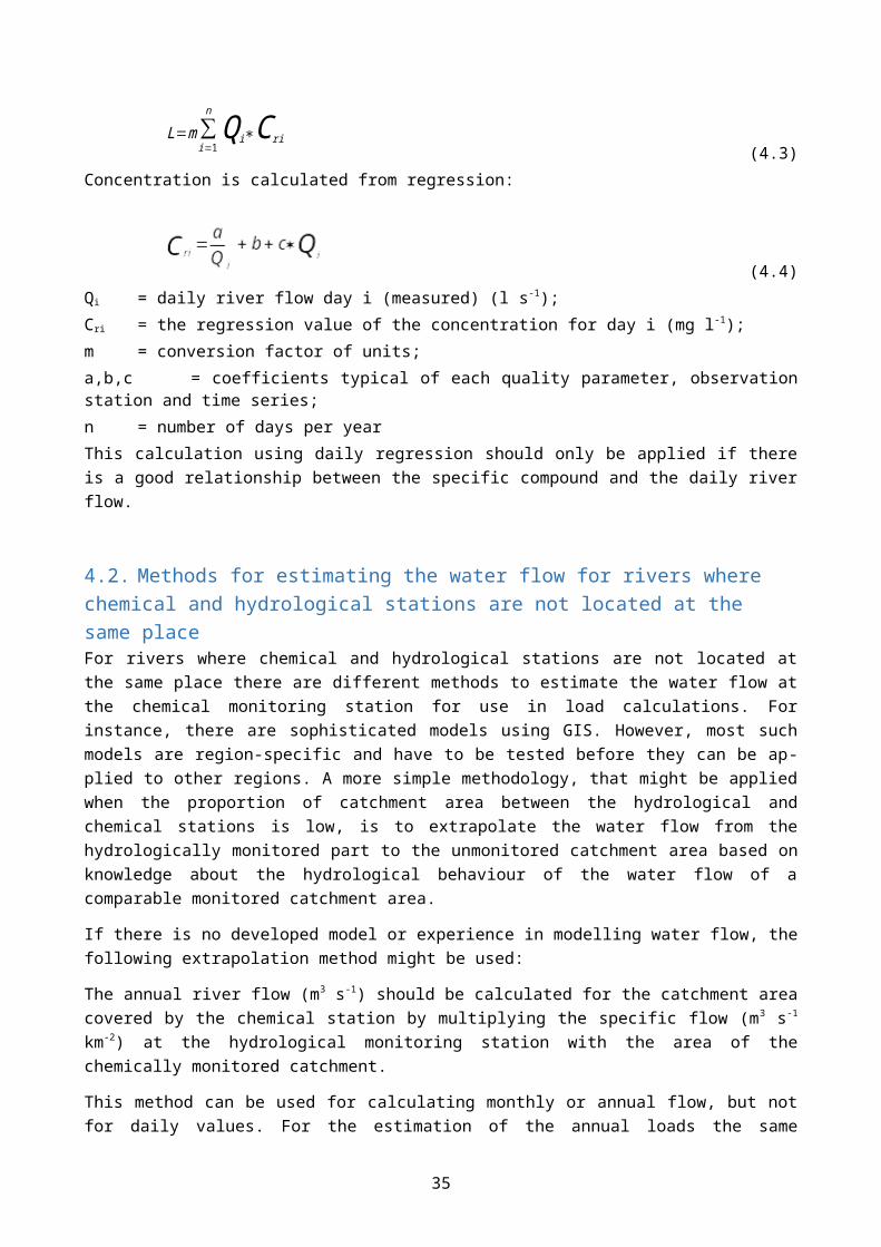
Daily river flow and daily concentration regression
Annual load (L) in kg a-1 is calculated as:
L=m∑i=1
n
Q i∗C ri (4.3)
Concentration is calculated from regression:
(4.4)Qi = daily river flow day i (measured) (l s-1);Cri = the regression value of the concentration for day i (mg l-1);m = conversion factor of units;a,b,c = coefficients typical of each quality parameter, observation station and time series;n = number of days per yearThis calculation using daily regression should only be applied if there is a good relationship between the specific compound and the daily river flow.
4.2. Methods for estimating the water flow for rivers where chemical and hydrological stations are not located at the same placeFor rivers where chemical and hydrological stations are not located at the same place there are different methods to estimate the water flow at the chemical monitoring station for use in load calculations. For
24

instance, there are sophisticated models using GIS. However, most such models are region-specific and have to be tested before they can be applied to other regions. A more simple methodology, that might be applied when the proportion of catchment area between the hydrological and chemical stations is low, is to extrapolate the water flow from the hydrologically monitored part to the unmonitored catchment area based on knowledge about the hydrological behaviour of the water flow of a comparable monitored catchment area.
If there is no developed model or experience in modelling water flow, the following extrapolation method might be used:
The annual river flow (m3 s-1) should be calculated for the catchment area covered by the chemical station by multiplying the specific flow (m3 s-1 km-2) at the hydrological monitoring station with the area of the chemically monitored catchment.
This method can be used for calculating monthly or annual flow, but not for daily values. For the esti mation of the annual loads the same equations as in Chapter 4.1 should be used. If other methodologies are applied, information about the used methodology should be reported (cf. annexes 2 and 3).
25

5. Quantification of load from point sourcesThis chapter covers calculation and estimation methods to quantify the load from point sources (municipal wastewater treatment plants, industrial plants and aquaculture plants) into recipient water bodies (defined as monitored areas, unmonitored areas or directly to the sea). It should be noted that if a point source has several outlets, located in different sub-basins, the load should be presented separately for each outlet. Details on wastewater sampling and flow measurement are provided in Chapter 3, and on reporting requirements in Chapter 13.
5.1. Municipal Wastewater Treatment Plants (MWWTP)The wastewater outflow should be measured continuously in order to calculate the total volume in a certain time period (day, month, and year). Furthermore, the wastewater samples should be taken frequently as flow-weighted composite samples. If that is not possible, the monitoring programme has to be optimized (see Chapter 3 for details concerning wastewater monitoring and sampling). Annual discharges should be calculated as the product of annual total quantity of wastewater and flow-weighted concentrations; the three ISO standard methods below (a, b and c) are examples of such quantification procedures. Where there is no reliable monitoring method, the load may be derived from per capita load estimates (d).
a) Continuous flow measurements and sampling (e.g. 24 hours flow-weighted composite samples 7 times/week)
The annual load in kg a-1 is the cumulative load of continuously monitored time periods and can be calculated as follows:
L=∑i=1
n
Qi ¿Ci* 0.001 (5.1)
L = annual load (kg a-1)Qi = wastewater volume of period i (m3)Ci = flow weighted concentration of period i (mg l-1)n = number of day in the year
b) Continuous flow measurement and non-continuous sampling every second day, once a week or twice a month (preferably as 24 hour composites)
The annual load can then be calculated as follows:
L=∑i=1
n
Qi∗C i
∑i=1
n
Q i
∗Qt
*0.001 (5.2)
L = annual load (kg a-1)Qi = wastewater volume of period i (m3)Ci = concentration of sample i (mg l-1)Qt = total wastewater volume of the year in m3
n = number of sampling periods
26

c) Flow measurement only on sampling days and sampling rather seldom i.e. 1–12 times per year
In this case the annual load can be calculated by multiplying the average load of sampling days by 365, as follows:
L=∑i=1
n
Qi∗C i
n∗365
*0.001 (5.3)
L = annual load (kg a-1)Qi = wastewater volume on sampling day i (m3)Ci = concentration on sampling day i (mg l-1)n = number of sampling days
d) Load estimate of small MWWTPs (<2,000PE) and for untreated sewage discharges without reliable monitoring
If no reliable monitoring has been done for small MWWTP (<2,000 PE) or for untreated sewage discharges and only population data (PE) are available, the load may be derived on the basis of the below per capita load estimates:
BOD5 1 PE = 60 g O2/day (70 g O2/day for BOD7)
Ntotal 1 PE = 12 g N/day
Ptotal 1 PE = 2.7 g P/day
However, countries should use their own estimates if more specific data on the local conditions are available. These estimates, including the calculation methods used, must be reported (see chapter 13 on annual reporting).
During storm events, combined sewers3 may not be able to treat all wastewater in the wastewater treatment plant due to heavy loads of rainwater. This may lead to either an overflow 4 in the sewage system or that the water is discharged directly to surface water via a bypass5. These portions need to be quantified and the related nutrient loads estimated.
Note! When the drainage water from paved areas etc. are treated separately (i.e. not included in a combined sewage system), the nutrient load via the drainage water should be included among the diffuse sources as this kind of sources often do not have a distinct outlet.
5.2. Industrial plants (INDUSTRY)Industrial plants may discharge industrial effluents to the Baltic Sea,
directly, indirectly via other recipient water bodies (e.g. river, stream, creek) or,
3 Combined sewage system includes both wastewater and drainage water from paved areas etc.. Control of overflows is regulated with HELCOM Recommendation 23/5.4 Overflows are discharges from combined sewerage system to the water body during rainfall when the flow (mixture of sewage and rainfall runoff) in the system is over-loading the designed volume of the system. Control of overflows is regulated with HELCOM Recommendation 23/5.5 By-passes are discharges from a sewerage system to the water body to prevent station treatment plant overflow damages during breaks in electricity supply or emergency repairing works. Use of by-passes is regulated with HELCOM Recommendation 16/9.
27

indirectly via a MWWTP.
Direct discharges should preferably be reported plant by plant annually, but can be reported as a sum for every Baltic Sea sub-catchment.
Periodical reporting requires distinguishing discharges between monitored and unmonitored areas. Substances include Ntot, Ptot and Flow and heavy metals where monitoring is part of the plant operation permit.
Quantification of discharges from industrial plants to surface water may be done similarly to UWWTPs by multiplying annual total quantity of wastewater and flow-weighted concentrations. Information can be derived from the plant operator or from the permitting authority.
Minimum reporting should include plants/facilities, which have a significant impact on the environment. The significance is demonstrated by covering facilities that,
1. undertake one of the activities listed in Annex I (Categories of activities referred to in Article 10 of the EU Directive 2010/75/EU on industrial emissions)6,
2. and exceed the production capacity/output, 3. and exceed threshold values fixed for the release of substances.
Plants/facilities that fulfil these criteria have to report data to the European Pollutant Release and Transfer Register (E-PRTR)7 available at http://prtr.ec.europa.eu/. Data in this Register is of use in PLC and needs not to be recalculated. Non-EU countries applying other rules are invited to strive for good correlation to these criteria and to measurements and analytical methods complying with international standards.
However, differences and potential inconsistencies exist between data reported under different reporting obligations.
For completeness, any other plant with industrial effluents entering Baltic Sea and national catchment areas should be included in PLC.
Source identification and reporting details are in Annex 6 of these guidelines.
5.3. AquacultureThe term aquaculture refers to the cultivation of both marine and freshwater species (e.g. fish and shellfish) in either land-based systems that discharge either to rivers and inland lakes, through direct point sources or production systems in coastal and open-marine areas. In general, fish farms are the main concern regarding aquaculture as a nutrient source to the sea. On the contrary, shellfish cultures could be seen as having a net export of nutrients from the water, as the nutrient supply is from the water, and by harvesting the produced shellfish nutrients are actually removed from the system. Also some freshwater aquaculture plants can net retain e.g. phosphorus.
The main source for nitrogen, phosphorus and organic matter (measured as BOD) discharges from aquaculture is the feed supplied into the farming system. Cultivation of mussels and other species that do not use artificial feed are not covered in this guideline. Discharges of nitrogen, phosphorus and BOD (organic matter) are derived from uneaten feed, undigested nitrogen, phosphorus and organic matter
6 IED = EU Directive 2010/75/EU on industrial emissions. The IED was a recast of seven existing Directives related to industrial emissions into a single clear and coherent legislative instrument. The recast included in particular the IPPC Directive.7 PRTR = The European Pollutant Release and Transfer Register (E-PRTR) is the Europe-wide register that provides easily accessible key environmental data from industrial facilities in European Union Member States and in Iceland, Liechtenstein, Norway, Serbia and Switzerland. It replaced and improved upon the previous European Pollutant Emission Register (EPER).
28

(faeces), and excretion via gills and urine. Measures aimed at the reduction of discharges from freshwater and marine fish farming in specific, are regulated in HELCOM Recommendation 25/4 “Measures aimed at the reduction of discharges from fresh water and marine fish farming” (HELCOM 2004).
Discharges from aquaculture plants into rivers or lakes can be determined by:
1. monitoring at the outlets from these plants or2. through calculations. Calculations can be based either:
(1) on records of fish (or other farmed organism) production and feed used, or (2) by using feed conversion rates (FCR) combined with chemical analyses of feed and fish and taking into account removal of nutrients (and organic matter) by natural processes and sludge removal (for more information, see OSPAR 2004 and HARP NUT Guideline 2, 2004).
Quantification of discharges from fish farming plants may be based on aggregated information extracted from national registers of annual figures for relevant parameters from each individual plant. Such statistics are usually collected as part of the requirements in the discharge permits. For the quantification of discharges, the distinction is made between two main production types:
1. Plants without treatment (e.g. plants where the sludge is not collected or where the sludge is collected, but discharged to the aquatic environment without treatment); and
2. Plants with treatment (e.g. plants with permanent removal of sludge), where the N and P contents (and organic matter) in the sludge removed are quantified.
The quantification of discharges from aquaculture plants is described in the following three approaches:
1. Approach 1 is based on calculations from production parameters. The starting point is that information is available on both production and feed consumption at plant level. The quantification method is based on mass balance equations. Valid for both marine and freshwater aquaculture plants.
2. Approach 2 is based on calculations from production parameters, but only information on either production or feed is available at national level. Valid for both marine and freshwater aquaculture plants.
3. Approach 3 is based on monitoring the discharge. It is feasible for ponds or other land based production systems where the discharges are distinct point discharges (such as end of pipe/channel). The quantification of losses is also based on mass balance equations, but in this case on monitoring results. Valid only for freshwater aquaculture plants.
Approach 1 (marine and freshwater plants)
This approach forms a basis for the estimation of nitrogen, phosphorus and BOD (organic matter) discharges from aquaculture plants (Cho et al. 1991).
a) For plants without treatment (sludge removal):
Phosphorus (P) or nitrogen (N) discharge to water body in kg a -1 (L P/N)
LP/N = 0.01*(ICi-GCf)-M-T (5.4)
I = amount of feed used for feeding of fish in kg a-1
Ci = P or N content in feed in %
29

G = net growth of fish including dead fish in kg a-1
Cf = P or N content in fish in %
M = nutrient losses due to metabolism in fish in kg a-1
T = nutrient removal processes on the fish farm not related to sludge removal (e.g. nutrient turnover, denitrification etc.) in kg a-1
BOD discharge to water body in kg a -1 (L BOD)
LBOD= (PL–D) (5.5)
PL = Internal fish farm loss from fish production
= (686-1671*Fk +1544*Fk2 -354*Fk
3)*G (5.6)
Fk = I/G feed quotient, i.e. feed used for producing fish during a year
I = amount of feed used for feeding of fish in t a-1
G = net growth of fish including dead fish in t a-1
D = area-decomposition/turnover of BOD = Ed * A (5.7)
Ed =specific decomposition/turnover in kg m-2 a-1
= (6.4 * Fk – 4,2) * 0.365 (5.8)
A = water covered surface area in the fish farm (estimate of the sedimentation basin surface area and of the plant lagoon, if present) in m2
b) For plants with treatment (sludge removal):
Phosphorus (P) or nitrogen (N) discharge to water body in kg a -1 (L P/N)
LP/N =0.01*(ICi-GCf)-M-T-S (5.9)
I = amount of feed used for feeding of fish in kg a-1
Ci = P or N content in feed in %
G = growth of fish in kg a-1
Cf = P or N content in fish in %
M = nutrient losses due to metabolism in fish in kg a-1
T = nutrient removal processes on the fish farm not related to sludge removal (e.g. nutrient turnover, denitrification etc.) in kg a-1
S = amount of P or N removed with the sludge in kg a-1
BOD discharge to water body in kg a -1 (L BOD)
LBOD = (PL – D) * (1 – S) (5.10)
PL = Internal fish farm loss from fish production = (686-1671*Fk+1544*Fk2-354*Fk
3)*G (5.11)
Fk = I/G feed quotient, i.e. feed used for producing fish during a year
I = amount of feed used for feeding of fish in t a-1
30

G = net growth of fish including dead fish in t a-1
D = area-decomposition/turnover of BOD = Ed * A (5.12)
Ed = specific decomposition/turnover in kg m-2 a-1
= (6.4 * Fk – 4.2) * 0.365 (5.13)
A = water covered surface area in the fish farm (estimate of the sedimentation basin surface area and of the plant lagoon if present) in m2
S = reduction factor for nutrient removal processes on the fish farm not related to sludge removal.
The net growth (G) of one year in equations 5.4, 5.5., 5.9 and 5.10 is calculated as the sum of i, ii, and iii below + the difference between the standing stock by the end of the year and the beginning of the year:
i. organisms taken out of the water for slaughter (alternatively the sum of slaughter weight and slaughter offal) or sold alive (t a-1)
ii. dead organisms collected during the year (t a-1), and
iii. escaped organisms (t a-1).
The total nitrogen and phosphorus content in the feed may be obtained from the feed manu facturers. In order to facilitate national calculations, average figures based on the typical feed used in the catchment area may be used, but if the type(s) of feed in each individual fish farm is known ideally that information should be used. The indicative figures in Table 5.1 may be used if the above mentioned figures are not available. If “moist/semi-moist feed” (higher content of water than “dry feed”)8 is used, the quantity of moist/semi-moist feed should be converted to the comparable amount of dry feed, as an expression of the total quantity of feed used. The total phosphorus and nitrogen content in the produced organisms can be obtained as a standard figure for each catchment area. If such figures are not available, the figures in Table 5.1 may be used.
Table 5.1. Content of nitrogen and phosphorus in fish and fish feed.
Total phosphorus content (%) Total nitrogen content (%)
Fish (fresh) 0.4 2.5
Dry feed 1 1.0 7.5
Semi-moist feed 2 0.5 5.0
Moist(fresh) feed 3 0.45 2.5
1 Dry matter >80 % 2 Dry matter 35-80 % 3 Dry matter <35 %
The calculation of treatment yield requires that the nitrogen and phosphorus content in the sludge is calculated/measured regularly (e.g. based on requirements in the discharge permits) as basis for quantification of the fraction that is removed by the sludge. If such figures are unavailable and, in the case
8 The water content in this feed category varies, but a general guidance can be: semi-moist feed (35-80% is dry matter), moist feed (< 35% is dry matter), while a dry feed has > 80% dry matter.
31

of regular removal of sludge, an average removal of 10% N and 40% P due to decantation may be considered.
Approach 2 (marine and freshwater plants)
If national registers on feed use and production on individual plants are not available, national sales statistics could be used. If only statistics on production or feed used is available, an assumption of the feed conversion ratio (FCR) should be made. FCR is the ratio between weight of feed used (dry feed basis) and weight gain of the organism (production), expressed as:
FCR = Feed used (t a -1)Production (ta -1)
(5.14)
The FCR is, among other things, species dependant and varies also by water temperature, as the fish metabolism is temperature dependent. Hence, it is preferred to use FCRs specific for the actual catchment or region based on estimates obtained from literature or determined from experimental work. If literature values are used, the report should include a literature reference. If no values from literature or experimental work are available the following standard figures are recommended:
FCR=1.1 for big fish over 0.8 kg (although use 3.0 for mother fish ) FCR=0.8-1.0 for fish between 30 g and 800 g FCR=0.6 for fingerlings
The figures are obtained from salmonid fish production under optimal growth conditions. Other figures should be used for other fish. When FCR is available for the catchment/region to be reported on, the missing figures of feed used or production may be estimated from the above-mentioned equation (equation 5.14). Method 1 can then be followed for the quantification of the discharge.
Approach 3 (freshwater plants only)
For land-based aquaculture systems such as artificial ponds, basins and raceways, the nitrogen and phos -phorus discharges may be quantified by monitoring the nitrogen and phosphorus concentrations and the water flow in the inlet(s) and outlet(s) of the production system, followed by a mass balance calculation of the increased discharge. The discharge of nitrogen and phosphorus (and organic matter) from a production system may vary considerably over both the short and long timescale and depend, inter alia, on operational factors such as standing stock, application of feed, feed quality, time of feeding, time of cleaning operations, the presence of different purification tools and their effectiveness (e.g. plant lagoons are less effective during a cold winter), as well as on the natural variation in the inlet(s) water quality. The effluent monitoring strategy must reflect this variation.
All fish farming (or other aquaculture) plants with an annual production of more than 200 tonnes should, ideally, take as a minimum 12 contemporary samples a year in the inlet(s) and the outlet(s) for measurements of nitrogen and phosphorus concentrations.
In order to ensure a reliable quantification, sampling of water for analyses of nitrogen and phosphorus (and organic matter) should be flow-proportional over at least 24 hours and be carried out using automatic samplers.
Further, at least flow in inlet(s) and outlet(s) should be monitored on sampling days, but ideally monitored continuously providing daily water intake and outflow.
32

Good international laboratory practices, aiming at minimizing the degradation of samples between collection and analysis should be applied. The water flow should be registered continuously. Flow measurements should preferably be performed according to international standards (e.g. ISO standards).
The annual load of inlet(s) and outlet(s) may be calculated as follows:
L=∑i=l
n
Qi∗C i
∑i=l
n
Q i
∗Qt
(5.15)
L = annual load;
Qi = wastewater volume of the period i;
Ci = concentration of sample i;
Qt = total wastewater volume of the year;
n = number of sampling periods.
The total load of nitrogen or phosphorus (or organic matter) from the production system is calculated by deducting the total nitrogen or phosphorus load in the inlet(s) from the total nitrogen or phosphorus load in the outlet(s).
If flow and concentrations in inlet(s) to and outlet(s) from aquaculture plants are monitored regularly the method “Daily river flow and daily concentration (interpolated)” in Chapter 4.1 should be used (Eq. 4.1).
33

6. Quantifying diffuse losses of nutrientsDiffuse sources of nutrients are defined as any source of nutrients not accounted for as a point source. Within the periodic PLC-Water, quantifications of natural background and major diffuse anthropogenic nutrient losses to inland surface waters and to the sea are required (Chapter 14). In the annual reporting, the diffuse inputs are included in the total inputs from monitored rivers and unmonitored areas (cf. Chapter 13).
6.1. Quantification of the natural background nutrient lossesProcedures for the periodic quantification of natural nitrogen and phosphorous background losses into inland surface waters are described below. Natural background losses cover:
Losses from unmanaged land; and Part of losses from managed land that would occur irrespective of anthropogenic, e.g. agricultural,
activities.
Hence, the natural background losses are a part of the total diffuse losses. The Contracting Parties can use two different approaches or a combination of the approaches to estimate natural background losses:
Monitoring of small unmanaged catchment areas without or with very minor inputs from point sources, and/or
Use of models.
When background losses are estimated by models it is assumed that the anthropogenic surplus is zero, implying e.g. that the prevailing atmospheric nitrogen deposition needs to be taken into consideration.
Natural background losses of nutrients are monitored in several countries. The figures given in Table 6.1 are related to the period 1990-2000 besides data from Denmark that covers 1989-2012. They are obtained from forested catchment areas and/or catchment areas with very low human impact (with the exception of the impact of atmospheric deposition).
Table 6.1. Annual natural background losses and flow-weighed concentrations of nutrients as reported by Contracting Parties.
Country Total Nitrogenin kg ha-1
Total Nitrogenin mg l-1
Total Phosphorusin kg ha-1
Total Phosphorusin mg l-1
Waterflow inl (s . km2) -1
Denmark 2.64±±0.312 1.53±±0.061 0.086±±0,0112 0.050±±0.0021 6.19±±0.611
Estonia 3.3 1.1 0.12 0.04Finland 0.7-2.0 0.03-0.7Germany 1.23 0.733 0.061 0.036Latvia 0.11Lithuania 0.6-1.2 0.32-0.8 0.02-0.08 0.05-0.09 6.6Poland 1.5 0.1Sweden 0.33-2.8 0.013-0.0651 The average of median monitored values for 24 years (1989-2012) ± 2 SE (SE is the standard error, and the expressions corresponding to the 95% confidence interval) in seven small catchments without or with very low human activities.2 The average of median monitored values for 21 years (1989-2009) ± 2 SE in seven small catchments without or with very low human activities.
34
6.2. Quantification of nutrient losses from diffuse anthropogenic sourcesDiffuse anthropogenic nitrogen and phosphorus losses from the following sources should be considered in the quantifications:
Agricultural land Managed forestry and other managed land Atmospheric deposition directly on inland surface waters Scattered dwellings Rainwater constructions (e.g. paved surfaces without a distinct outlet)
Whereas point sources (defined as wastewater treatment plants, industrial plants and aquaculture plants) are discharging into inland surface waters or directly to the sea with a defined outlet, losses from diffuse sources (agriculture, forestry, atmospheric deposition, scattered dwellings, and rainwater constructions) may be delivered via a number of different pathways into inland surface waters (in monitored and unmonitored areas). Small, dispersed point source discharges e.g. from point sources in agriculture (e.g. farmyards) should also be dealt with as diffuse sources as long as they do not have a distinct and monitored outlet (in which case, they would instead be treated as a point-source). The pathways to inland waters are characterized by different flow characteristics and include very different processes (see Figure 2.2). Depending on the land use, losses of phosphorus and nitrogen can vary substantially. PLC-Water defines and considers the following seven diffuse pathways:
Surface run-off Erosion Groundwater Tile drainage Interflow9
Atmospheric deposition on inland surface waters Rainwater constructions Scattered dwellings
A large number of removal, storage or transformation processes may influence the final quantities of nitrogen and phosphorus entering inland surface waters. Knowledge about these processes of transformation and retention within inland surface waters is necessary to quantify and to predict nutrient losses into river systems in relation to their sources.
The different loss processes and pathways are very complex and variable, and the significance of their effects also varies between nitrogen and phosphorus. It is therefore difficult to quantify diffuse losses in a consistent and accurate way. The PLC-Water guidelines are not including a specific methodology for quantifying diffuse sources or delivery pathways. There are many different methodologies, e.g. OSPAR HARP-NUT Guideline 6 on diffuse sources (OSPAR 2007; only existing as a draft version that has not been finalized). In the absence of comprehensive measurements, it is necessary to apply calculation methodologies (e.g. various modelling techniques).
6.2.1.Documentation on used estimation methods for diffuse sourcesProcesses and pathways widely differ. There exist many different methods to estimate the loss from diffuse anthropogenic sources, it is vital that the Contracting Parties comprehensively describe the methodology used for various sources to ensure transparency and to enable assessments. It is important that the documentation include how e.g. the following important factors have been taken into consideration:
9 Substance transport within the vadose zone, i.e. unsaturated soils above the groundwater table.
35

Seasonal variation Retention (see chapter 9) Monitoring data as support to model or values from look-up tables or expert judgement Estimates based on source-oriented (sources are estimated) or load-oriented approach (only total
diffuse anthropogenic sources) – see also Chapter 10
There exist many different source-apportionment models, with varying capabilities to model the nutrient flow under various conditions, and with very different demands on supporting data. Some examples on commonly used models are given in Table 6.2. More examples are given in documentation from the EUROHARP project, in which thorough descriptions, as well as comparisons and assessments of commonly used models, can be found (e.g. Schoumans and Silgram 2003, and in 10 articles in Journal of Environmental Monitoring Vol. 11, pages 503–609 e.g. Hejzlar et al. 2009, Kronvang et al. 2009, Schoumans et al. 2009a, Schoumans et al. 2009b, and Silgram et al. 2009).
Important issues that need to be considered before a model is chosen are e.g.:
the purpose with the modelling (only source-apportionment or also scenarios on remedial measures?)
coverage of important pathways for the nutrients in the prevailing conditions supporting data availability compared to model needs source availability regarding man-power or financial support compared to what is expected for
data and model handling result assessment
Other important issues are temporal and spatial resolution (vertical and horizontal), high resolution generally implicate higher requirements on supporting data as well as higher labour demands, but maybe one of the most important issues is the applicability of the various models to the specific prevailing conditions that are to be modelled. If there are resources enough, it might be suitable with an ensemble modelling, i.e. several models are used and assessed together, to get more reliable estimates. More detailed concerns on various issues prior to start modelling may be found in e.g. Schoumans and Silgram (2003).
For documenting a model, the issues listed above should be described including a description of the process involved in the model and results of sensitivity and uncertainty analysis.
36

Table 6.2. Examples on source-apportionment models that may be used to estimate various nutrient sources and nutrient retention in different scales. Physically based model intend to describe relevant process in a physically correct way, while conceptual models are more or less based on empirical information. Physical models are generally relatively data demanding.
Name Type of model Model owner/origin
EUROHARP-NUTRET Retention only EUROHARP
FyrisNP ConceptualSLU, Sweden. Freely available for non-commercial purposes:http://www.slu.se/waterhub
HBV-NP Semi-Physical SMHI, Sweden; freely available10
HSPF Physical US. EPA downloadable:http://water.usgs.gov/software/HSPF/
HYPE Semi-Physical SMHI, Sweden, open source
MESAW Conceptual Grimwall & Stålnacke (1996)
MIKE BASIN Conceptual DHI, Denmark; commercial
MONERIS Semi-empiricalDownloadable:http://moneris.igb-berlin.de/index.php/model-structure.html
SWAT PhysicallyDownloadable public domain model: http://swat.tamu.edu/software/
Vollenweider Conceptual, retention only P lake model (Vollenweider 1975)
10 The model is being phased out by SMHI in favour of the HYPE model
37
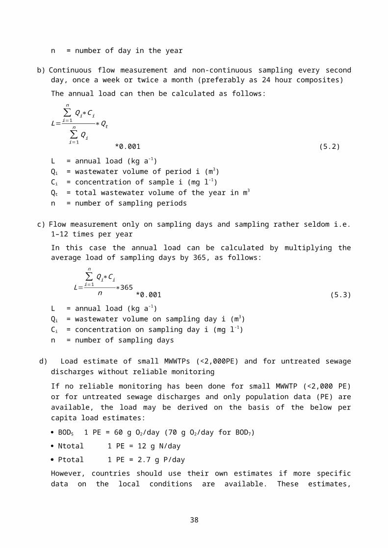
7. Methods for estimation of inputs from unmonitored areas Unmonitored areas consist of unmonitored rivers, unmonitored parts of monitored rivers and coastal areas including unmonitored islands (see Figure 2.4).
In unmonitored areas there are no available data on the requested water chemical determinands or on flow measurements in rivers. For such areas it is recommended to use one of the methods described below for estimating the loads (see also Chapter 6.2 on quantification of nutrient losses from anthropogenic diffuse sources). Alternative load calculation methods may be used, but must be described in detail (cf. annexes 2 and 3).
There are different methods to estimate the load from unmonitored areas:
Model results
Extrapolating the knowledge about neighbouring rivers under similar conditions.
If an unmonitored area has climate, topography, geology, soil type, land use etc. that are similar with a monitored area, also similar load in the output (river) can be assumed.
The following method should only be used if more sophisticated methods are not available and if the unmonitored part of the catchments only constitutes a minor share of the total catchment:
A rough calculation then takes into account only the different surface areas of the basins, e.g.:
(7.1)
Ln = input from unmonitored area An
Lm = known input coming from monitored area Am
An = area of unmonitored catchment
Am = area of monitored catchment
If possible the discharge from large point sources should be taken into account, as the discharges are rarely equal in the monitored area that is extrapolated to the unmonitored area. In some regions/countries the discharge from point sources is monitored and/or estimated also in unmonitored areas. Then the equation 7.1 above is changed to:
Ln=DLmAn
Am+PLU
(7.2)
Ln = estimated input coming from unmonitored area An
DLm = known diffuse inputs coming from monitored area Am (estimated as monitored load minus discharge from point sources taking into account retention)
PLu = monitored or estimated point source discharge from unmonitored areas;
An = area of unmonitored catchment
Am = area of monitored catchment.
38

Retention in surface waters within the unmonitored catchment should be taken into account when quantifying DLm and PLu.
Flow from unmonitored areas can be estimated with the methods described in Chapter 4.2.
39

8. Transboundary rivers
8.1. IntroductionThe Fifth Baltic Sea Pollution Load Compilation, PLC-5 (HELCOM 2011) addressed challenges related to transboundary nutrient inputs originating from countries both inside and outside the HELCOM area, as well as ensuring a fair allocation of pollution reduction burden in case of sharing transboundary watersheds between two or more HELCOM Contracting Parties. The initial calculations of nutrient inputs allocated riverine input to the country with the river mouth. This implies that e.g. Latvia and Lithuania are assigned the entire input via the Daugava and Nemunas to the Baltic Sea, respectively, while considerable proportions of these catchments belong to Belarus and Russia. Hence, there is a need for proper evaluations of the transboundary pollution inputs and to what extent these reach the Baltic Sea.
The follow-up system for the new CARTs, which was adopted at the Copenhagen 2013 HELCOM Ministerial Meeting (HELCOM 2013), require knowledge about transboundary riverine inputs from non-HELCOM Contracting Parties as well as between Contracting Parties to follow up on the progress towards reaching the nutrient reduction requirements. The new CARTs are specific for each Contracting Parties “own” share of the nutrient inputs to the Baltic Sea, and expected reductions in riverine inputs have also been allocated to non-Contracting Parties. Further, transboundary inputs between HELCOM Contracting Parties were taken into account when allocating the reductions requirements. Also the 2013 Copenhagen Ministerial Meeting underlined that transboundary nutrient inputs originating in the non-Contracting Parties should be addressed by initiating joint activities e.g. by bi- and/or multilateral projects and through other existing funding mechanisms as well as by international agreements such as the 1992 UNECE Convention on Transboundary Waters and Lakes, and the River Basin Management Plans of the EU Water Framework Directive for HELCOM Contracting Parties being also EU Member States.
Therefore, addressing transboundary inputs between Contracting Parties and non-Contracting Parties and between two or more Contracting Parties (including border rivers) has been identified as an important task for the HELCOM LOAD group and future PLC assessments. Further, quantifying transboundary inputs between countries can also be used to evaluate the importance of these inputs as a source to the receiving countries and to follow development in transboundary inputs. For assessing the importance of measures taken in upstream loading countries on the net inputs to the Baltic Sea, retention in downstream countries surface waters must be taken into account (see Chapter 9).
This chapter defines actual and net transboundary inputs, and includes an overview of the rivers that are identified as transboundary rivers. Further it includes border rivers and how they are defined. It also includes a short overview of information necessary for assessing actual and net transboundary inputs.
About 7% of the total catchment draining to the Baltic Sea (1.73 million km 2) is situated in non-Contracting Parties, but also a proportion of the catchment area within Contracting Parties contributes with transboundary riverine inputs to other Contracting Parties. Figure 2.5 shows the whole Baltic Sea catchment, illustrating the catchment area within HELCOM Contracting Parties as well as non-Contracting Parties.
8.2. DefinitionsA transboundary river is a river that crosses at least one country (political) border and has its outlet to the Baltic Sea in one of the HELCOM Contracting Parties. A transboundary river can cross more than one country, both between Contracting Parties and from a non-Contracting to a Contracting Party. Therefore,
40
riverine inputs can originate from one or more countries. To estimate net transboundary riverine inputs entering to the Baltic Sea, retention in inland surface waters must be taken into account (see Chapter 9).
A border river is a river with its outlet to the Baltic Sea at the border between two countries. For these rivers, the inputs to the Baltic Sea are divided between the countries in relation to each country’s share of total load.
Transboundary rivers are illustrated in Figure 2.4, which introduces and defines some main terms used in the PLC guidelines and as an example Figure 8.1, shows the lower part of the River Nemunas. River Nemunas have been classified as a transboundary river, and is regarded as a quite complicated case due to the fact that so many countries are involved in different parts of the catchment.
Figure 8.1. The lower part of the transboundary River Nemunas catchment. To the right from the map (not shown), Lithuania receives riverine transboundary inputs from the non-Contracting Party Belarus. In the central part of the map is the border between Russia (Kaliningrad Oblast) and Lithuania along the River Nemunas. There is also a river branch (with a quarter of the entire flow of Nemunas) – Matrosovka (or Gilija in Lithuanian) Channel – which transports transboundary inputs from Lithuania to Russia. The channel has an outlet to the Baltic Sea in Russia while the outlet of the main branch of the River Nemunas is in Lithuania (not at the border between Russia and Lithuania). Source: Google Earth, with some amendments.
41

8.3. Estimates of actual and net transboundary inputs used in the 2013 Copenhagen HELCOM Ministerial DeclarationAvailable data shows that the transboundary nutrient loads to the Baltic Sea are significant to some sub-basins of the Baltic Sea. However, the existing assessments have not so far enabled the evaluation of the significance of transboundary pollution accurately enough. Table 8.1 and Table 8.2 summarize estimates compiled by the Baltic Nest Institute, Sweden (BNI) (Gustafsson & Mörth, in prep.) on transboundary (actual and net inputs) divided between Contracting Parties and non-Contracting Parties (Table 8.1) and between Contracting Parties (Table 8.2) as used for calculating the new CARTs adopted by the 2013 HELCOM Copenhagen Ministerial Meeting (HELCOM 2013).
Table 8.1. Transboundary riverine inputs from non-HELCOM countries in the Baltic Sea catchment area (in tonnes per year) used in the CARTs calculations. All data are averaged 1997-2003 except for the Belarusian data which are averaged 2004-2011. Input at the border is reduced by the retention coefficient to estimate net waterborne input to the Baltic Sea (see Chapter 10). ‘Share of inputs to the sub-basin’ expresses (in %) how large a proportion of the total waterborne input to a sub-basin originates from the non-Contracting Party during the reference period. GUR = Gulf of Riga, BAP = Baltic Proper, GUF = Gulf of Finland, N = nitrogen, P = phosphorus. For more information, see Gustafsson & Mörth, in prep.
From Via To Border Retention To Baltic Share of input to the sub-basin
TN (t) TP (t) TN TP TN (t) TP (t) TN (%) TP (%)Czech Poland BAP 5,700 410 0.40 0.28 3,420 295 1.1 1.7Belarus Lithuania BAP 13,600 914 0.54 0.53 6,256 430 2.1 2.5Ukraine Poland BAP 4,124 127 0.40 0.28 2,474 91 0.8 0.5Belarus Poland BAP 5,071 331 0.40 0.28 3,043 238 1.0 1.4Total BAP 15,193 1,055 5.1 6.1Belarus Latvia GUR 8,532 1,360 0.27 0.32 6,228 925 7.9 41.4
Table 8.2. Transboundary riverine inputs between HELCOM Contracting Parties (in tonnes per year) in the reference period (1997-2003). The input at the border is reduced by the retention coefficient to estimate net waterborne transboundary inputs to the Baltic Sea. GUR = Gulf of Riga, BAP = Baltic Proper, GUF = Gulf of Finland, N = nitrogen, P = phosphorus. In the Finnish inputs to Gulf of Finland via Russia retention in Lake Ladoga has been taken into account. For more information, see Gustafsson & Mörth, in prep.
From Via To Border Retention To BalticTN (t) TP (t) TN (t) TP (t) TN (t) TP (t)
Lithuania Latvia BAP 5,516 158 0.39 0.58 3,365 66Poland Russia BAP 4,400 320 0.30 0.37 3,080 202
Germany Poland BAP 2,337 101
Total BAP 8,782 369
Lithuania Latvia GUR 7,185 282 0.27 0.32 5,245 192
Russia Latvia GUR 4,256 734 0.54 0.71 1,957 215
Total GUR 7.202 407
Finland Russia GUF 0.48 0.82 5,353 49
42

Data on sources in the non-Contracting Parties is still lacking and the available data does also not enable calculation of the share of pollution originating from the upstream countries that actually reaches the Baltic Sea as satisfactory estimates on retention in different individual rivers are not available.
If other (more) reliable data does not exist on retention within the catchment area, the results estimated in the EU-funded RECOCA project can be used (Gustafsson & Mörth, in prep.). These results are shown in Chapter 9 (Figure 9.1 and Table 8.2) and Annex 5. These retention coefficients can be used for calculation of net contribution of transboundary inputs from both Contracting and non-Contracting Parties at rivers mouths.
8.4. Necessary information for quantifying transboundary input The downstream HELCOM Contracting Party receiving riverine transboundary input from an upstream country (Contracting Party or not) and having the river mouth at the Baltic Sea is responsible to collect data, and to compile, quantify and report on the transboundary inputs. The downstream country is encouraged to cooperate with the upstream country in order to quantify loads and river flow at the border using the methods described in the PLC guidelines and to ensure that all relevant transboundary inputs are quantified and reported to the PLC-Water database. Further, Contracting Parties should also report on retention in the catchment receiving the transboundary input, if new data is available that differ from the one used for calculating the CARTs that were adopted in Copenhagen 2013 HELCOM Ministerial Declaration. For border rivers, the involved Contracting Parties should agree on the responsibilities above and report accordingly to HELCOM.
Necessary information to be used for estimating transboundary riverine inputs includes:
At the border and river mouth: annual water flow, total nitrogen, total phosphorus. Preferably also fractions of nutrients and heavy metals (see list of parameters in Chapter 3) to allow for quantifying actual annual transboundary inputs. Preferable this is based on monitoring. If the reported information has been modelled, then information on how the estimates were obtained should be reported
Name of the river and the location of the monitoring point(s) (geographical coordinates) Size of catchments in the up- and downstream countries Estimate of retention (in inland surface waters) on transboundary N and P input in receiving
Contracting Party, if any new information is available In periodic assessment of nutrient source quantifications: population in the catchment, point and
diffuse sources, information on land use, life stock, fertilizer application etc. (all in both the up- and downstream countries)
If a river crosses more than one country, all the information is needed from each country in order to enable separation of the information per country.
8.5. Overview of transboundary rivers to take into account in annual reporting This sub-chapter describes how transboundary inputs can be divided between Contracting Parties. The division for the biggest rivers is based on monitored inputs at the border where the river enters another Contracting Party and taking into account retention in the downstream Contracting Party receiving the transboundary inputs. For a few rivers, also the location of big point sources is taken into account. In a strict sense, there are 82 transboundary rivers, but for many of these almost the whole catchment is situated in one country only and for these the transboundary inputs are neglected.
43

Table 8.3 contains an overview of the transboundary rivers from which annual transboundary riverine inputs should be taken into account and net transboundary inputs should be estimated. The reported transboundary inputs will serve as input to the PLC assessments and to the annual follow-up of the BSAP nutrient reduction requirements adopted by the 2013 HELCOM Ministerial Declaration. The table provides information about the involved Contracting and non-Contracting Parties for each river, the division of the catchment, monitoring stations in HELCOM Contracting Parties at the border where transboundary riverine inputs enters, expected available information in upstream country etc. In addition, Table 8.3 also provides information on border rivers within the Baltic Sea catchment.
Note! This table will be reviewed and updated as new information becomes available.
44

Table 8.3 List of transboundary and border rivers that should be taken into account in annual and periodical PLC reporting:
River name
Transboundary/ border river between which CP’s/countries
CP to provide information and involved CP
Total catchment and proportion of catchment in involved countries
Monitoring station in CP and what is monitored
Expected available information in upstream country(ies)
Other comments
Narva Border and transboundary river
LV to RU; EE and RU, BY
EE (own catchment) and RU (LV and RU catchment)
Total area: 58,126 km2
EE: 30.2 %LV:6.3 %RU: 63.0 %BY: 0.5%
EE:2 hydrochemical stations (7 km from mouth and outflow from Peipsi),2 hydrological stations (20 km from mouth outflow from Peipsi )RU:chemical monitoring station -12 km from mouth; hydrological - 16 km
LV:No hydrochemical surveillance monitoring stations with annual measurements;1 hydrological – flow monitoring station (Zilupe – Pasiene)
RU to contact LV or to decide whether to take on LV load as part of RU inputs
Torne älv Border river between SE and FI
SE Total area:40,112 km2
SE: 63.9 %FI: 35.0 %NO: 1.2 %
SE: Chemical station at Mattila (approx. 7 km from outlet). Hydrological station at Kukkolankoski (approx. 20 km from outlet)Fi:
It is agreed that 55 % of the inputs of N and P entering the sea via the river is from SE and the remaining 45 % from FI
Gauja Transboundary riverEE/LV
LV Total area:8,950 km2
LV: 77.5 %EE: 12.5 %
LV:1 hydrochemical surveillance MS (Gauja, 2.0 km below Carnikava, mouth);1 hydrological – flow MS (Gauja – Sigulda)
EE:1 hydrological station and 1 hydrochemical station (river Mustjõgi, 4 km from LV border)
Lielupe Transboundary riverLI/LV
LV Total area:17,814 km2
LV: 50.4 %LT: 49.6 %
LV:Border MS:River Mūsa: 1 hydrochemical surveillance MS (Mūsa, on Latvia – Lithuania border); 1 hydrological – flow MS (Mūsa-Bauska);River Mēmele:1 hydrochemical surveillance MS (Mēmele, 0.5 km below
LT:4 chemical stations (rivers Platone, Sidabra, Musa ir Nemunelis) and 7 hydrological stations (rivers Svete, Platonis, Sidabra, Yslykis, Musa, Nemunelis 2 stations) near the LT/LV border
45

Skaistkalne); 1 hydrological – flow monitoring station – data from LT (Mēmele – Tabokine);Mouth MS:River Lielupe:1 hydrochemical surveillance MS (Lielupe, 0.5 km below Kalnciems); 1 hydrological – flow monitoring station (Lielupe-Mežotne)
Oder Transboundary riverCZ/DE/PL
PL Total area:118,840 km2
CZ: 6.1 %DE: 4.7 %PL: 89.2%
PL:1 station with hydrological and hydrochemical measurements (Krajnik,71.9 km from the mouth)
DE:2 hydrochemical stations (one of them on PL border), 3 hydrological stationsCZ:1 station with hydrological and hydrochemical measurements (border station, Chalupki 741.9 from the mouth)
Neva Transboundary riverBY/FI/RU
RU Total area: 281,000 km2
BY: 0.3 %FI: 20.2 %RU:79.5 %
RU:mouth hydrological station – 27 km from mouth and 4 chemical stations in each branch of Neva river (one-in 1.4 from mouth, three – in 0.025 km from mouth)
Pregolya Transboundary riverLT/PL/RU
RU Total area: 15,500 km2
LT: 0.6 %PL: 51.1 %RU:48.3 %
RU:chemical monitoring station -1 km from mouth; hydrological -≈50 km and includes only nutrient fractions (P-PO4,N-NO2...etc)PL:PL Monitoring stations: Lyna 73.7 km (lack of flow data since
PL:In PLC-5.5 PL loads were calculated based on data from the river Lyna and Wegorapa with using average flow from years 1994-2003 and 2006)
46

year 2007;Wegorapa 96.5 km (lack of flow data since 2007)
Venta Transboundary riverLT/LV
LV Total area: 11,692 km2
LT: 44.3 %LV:55.7
LV:Border MS:1 hydrochemical surveillance MS (Venta, 0.5 km below Nīgrande) ;Mouth MS : 1 hydrochemical surveillance MS(Venta, Vendzava, hidroprofils).1 hydrological – flow monitoring station (Venta-Kuldīga).
LT:3 chemical stations (rivers Varduva, Venta, Vadakstis) near the LT/LV border and 1 hydrological station (river Venta)
Barta Transboundary riverLT/LV
LV Total area:2,016 km2
LT: 37.1 %LV: 62.9 %
LT: 1 chemical station and 1 hydrological station in the Bartuva river near the LT/LV border
Daugava EE/LT/RU/BY/LV LV Total area: 87,900 km2
EE: 0.2%LT: 2.2 %RU: 31.6 %BY: 38.2 %LV: 27.7 %
LV:Border MS:1 hydrochemical surveillance MS (Daugava, Piedruja, Latvia - Belarus boder);1 hydrological – flow monitoring station (Daugava-Daugavpils)Mouth MS : 1 hydrochemical surveillance MS(Rīga reservoir, 1.0km below Lipši) ;1 hydrological – flow monitoring station (Daugava-Jēkabpils).
RU:chemical monitoring station at the RU/BY border;LT:1 chemical and 1 hydrological station at the LT/BY border in the river Birveta (around 3 km away from the border) and 1 chemical and 1 hydrological station in the river Dysna (around 1.5 km away from the border)EE:river Pedetsi, no
47

monitoring
Nemunas RU/LV/BY/PL/LT LT Total area: 97,920 km2
RU: 1.6 %LV: 0.1 %BY: 47.1 %PL: 2.6 %LT: 48.6 %
LT:2 chemical and 2 hydrological stations at the LT/BY border (one of each in the Nemunas river around 10 km away from the border and in the Neris river around 2 km away from the border).5 hydrological and 4 chemical stations are on the LT/RU border in the Nemunas river. Last one around 8 km from the mouth.RU:2 chemical stations: 1st in the Nemanus river in 59 km from mouth; 2nd in the Matrosovka canal in 24 km from mouth (monitoring includes only nutrient fractions (P-PO4,N-NO2...etc)
LT:Sesupe river at the LT/RU border has 1 chemical and 1 hydrological station.
Vistula BY/UA/SK/PL PL Total area: 194,424 km2
BY: 6.5 %UA: 5.7 %SK: 1.0 %PL: 86.7 %
PL:Polish loads (Kiezmark 12km from the mouth)Loads from BY (Monitoring stations on the Bug river 222.0; 227.5 and 291.0km and Narew river 44.6 km)Loads from UA (monitoring station on Bug river 578.1km)
PL:No (BY, UA, SK)
PL:Bug river, (transboundary and borer river with BY and UA). For PLC-5.5 loads were estimated basing on own data )
Göta älv NO/SE SE Total area: 50,233 km2
NO: 16.7 %SE: 83.3 %
SE: Sweden to investigate the availability and continuity of point source and land use data during the PLC-6
SE: Currently (and in previous PLC deliveries), Sweden has treated the load entering the sea from these areas as negligible due to low anthropogenic pressures in the
48
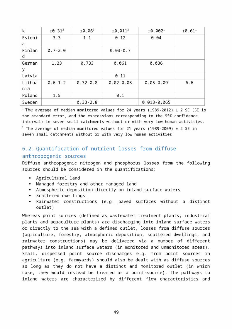
project mountainous areas of all these rivers and high retention in lakes between these regions and the sea. Sweden will evaluate this approach within the PLC-6 project, investigating the availability and continuity of point source and land use data and the expected nutrient retention in lakes and water courses.Based on these estimates, a decision will be taken as to whether to maintain the current approach (which assumes that the Norwegian contribution to the total load from each of these three rivers is negligible compared to the Swedish loads) or whether this approach should be re-evaluated and the rivers treated as conventional transboundary watercourses.
Indalsälven
NO/SE SE Total area: 26,726 km2
NO: 7.9 %SE: 92.1 %
SE: SE: Sweden to investigate the availability and continuity of point source and land use data during the PLC-6 project
Ångermanälven
NO/SE SE Total area: 31,864 k m2
NO: 4.9 %SE: 95.1 %
SE: SE: Sweden to investigate the availability and continuity of point source and land use data during the PLC-6 project
Coast LV/Baltic Proper
LT/LV LV Total area: 5,257 km2
LT: 14.2 %LV: 85.8 %
LV:Bārta river:Border MS:1 hydrochemical surveillance MS (Bārta, Latvia - Lithuania border);Mouth MS : 1 hydrochemical surveillance MS(Bārta, 0.2 km above Dūkupji, hidroprofils).1 hydrological – flow monitoring station (Bārta-Dūkupji).
LT:Bartuva is included separately in this list. There are no more significant transboundary coastal catchments shared between LT and LV
Coast RU/ PL/RU RU Total area: 1,538 km2
49

Baltic Proper(RU: Propose to refer this section to Mamonovka and Prokhladnaya rivers)
PL: 25 %RU: 75 %
Coast RU/Gulf of Finland
FI/RU RU Total area: 2,715 km2
FI: 59 %RU: 41 %
RU: chemical station on river Seleznevka – 12 km upstream mouth; hydrological station – 25 km upstream mouth.
Salaca LV/EE LV Total area 3,471 km2
LV: 91.9 %EE: 8.1 %
LV:1 hydrochemical surveillance MS (Salaca, 0.5 km above Salacgrīva) ;1 hydrological – flow monitoring station (Salaca-Lagaste).
50

9. Quantification of nutrient retention
9.1. IntroductionRetention of nitrogen and phosphorus in surface waters (lakes, rivers including flooded riparian zones) is a process that permanently removes nitrate through denitrification or stores of nitrogen and phosphorus for shorter or longer time periods in sediments and vegetation thus delaying the nutrient transport in river basins. In some cases retention can even be negative due to the release of nutrients from lake and river sediments. In general, phosphorus retention is influenced by sedimentation and other physical and chemical processes, while nitrogen retention to a large extent is influenced by biological processes.
Retention needs to be estimated in order to enable quantification of sources of nutrients to marine areas from different parts of river basins. A geographically detailed estimate of retention will make a reliable source apportionment of the inputs to the sea possible, which in turn will enable efficient water protection measures. Ideally, if individual evaluation of all different measures and sources are expected, retention should be estimated separately for all categories of nutrient sources in a river system, also taking into account the distance to the coast.
If the loads from agriculture are expressed as losses from the root zone, the retention estimates will also include soil retention, i.e. removal processes that occur in soil and groundwater. These guidelines only deal with retention of phosphorus and nitrogen in inland surface waters, which is also the reporting obligation for the PLC periodic assessments.
9.2. QuantificationThe total retention in the river catchment (R) is the sum of retention for each source category, expressed as:
R = Rp + RD + RB (9.1)
Where Rp, RD and RB is retention for point sources, diffuse sources and background load, respectively (t a -1).
It is generally difficult to distinguish retention from the different sources in equation 9.1. The calculation can be simplified if it is assumed that retention is proportional to the total load of each source and that the retained fraction is the same for all sources. Then only the total retention (R) is needed. Further, the procedure outlined above requires measurements at one or several monitoring sites of the selected river in order to determine riverine load (can be a normalized riverine load). It also requires data on nitrogen and phosphorus point source discharges and natural background losses in the river catchment area. If there is a significant degree of uncertainty in the retention estimate, more than one retention methodology or a sensitivity analysis should be applied to get a range for the quantification of diffuse sources entering inland surface waters.
The following main quantification approaches can be used:
A. Mass balance approachB. Modelling approach
A. Mass balance approach
This approach is based on monitoring data from inland waters, used to calculate mass balances for selected parts of the river system. The method can be applied to:
51

the whole river catchment lakes, (use results on lakes retention from parts of the catchment for lakes in the remaining
part of the are scaled to the whole catchment sub-catchments covering the whole catchment
Basically the methodology is the same irrespective of the size of the calculation unit. The retention is calculated as the difference between the input and output of the considered water body, preferably on an annual basis, according to the equation:
(Ia +lb + Ic + In) - U = R (9.2)
Where Ia – In are input sources, U is Output and R is retention.
Estimates of diffuse inputs based on a longer time period (more than one year) will result in a retention estimate for the corresponding period.
Estimation using equation 9.2 can be simplified by ignoring small input sources. Another simplification can be made by analyzing only a few sub-catchments representing different parts of the river system and transforming the results to the whole river. If possible, retention in big lakes should always be assessed separately
The simplest way of calculating total retention in a catchment is to make a mass balance for the whole river system and calculate retention as the difference between the sum of all inputs at source (gross load) from the load calculated at the river mouth station (net load). A major problem with this approach is that it only gives an average retention figure for the whole river system. Retention may differ between sources positioned in different parts of the catchment, and thus the source apportionment at the coast will not be precise. For small rivers this difference may be less important. When applying the mass balance approach to larger river catchments the calculations become more complicated and the use of numerical models may be necessary.
B. Modelling approach
A modelling approach is often applied when retention is calculated in a river system for the whole catchment or for sub-catchments. The retention is calculated with empirical or dynamical models covering from mass balance models to algorithms describing the relationship between retention and river characteristics. The selected model should preferably be able to calculate retention of individual sub-catchments as well as for the whole river system.
There are several, both freely available and commercial, models that can be used to calculate retention. They all need input data on point and diffuse nutrient sources as well as river and lake characteristics. Some available models are described in Table 6.2. They have variable applicability depending on e.g. the scale and climatologically conditions of the study catchment. In the EUROHARP project several models compiling retention have been compared regarding their retention estimates and the results are published in Hejzlar et al. 2009.
9.3. Available retention dataWhere available, retention data provided by Contracting Parties has been used. If such data have not been available, then e.g. results estimated by projects such as RECOCCA were used for estimating net transboundary inputs.
Several studies have been made in different Baltic Sea countries to estimate nutrient retention. One example is the RECOCA project (2009-2012) in which total and surface water nutrient retention of the major river catchments around the Baltic Sea were calculated. Total retention, including both soil and water
52
retention, were estimated using a regional mass balance model (Hong et al. 2012). The results show quite high retention values for the largest catchments of the Baltic Sea (50-86% for total nitrogen and 85 to nearly 100% for phosphorus). Nutrient retention in surface waters (river and lakes) was also calculated for all major river catchments around the Baltic Sea using the MESAW model (Stålnacke et al. 2003). Both retention datasets from the RECOCA project are available from BNI-Sweden.
Retention estimates of transboundary inputs should only contain retention in rivers and lakes. Inputs and retention coefficients of transboundary inputs were compiled during the revision of MAI and CARTs for the BSAP (see Table 8.1 and 8.2, and Figure 9.1).
Figure 9.1. The nitrogen and phosphorus surface water retention coefficients used to estimate waterborne transboundary inputs by the RECOCCA project (cf. Chapter 8.3). The retention data calculated by RECOCCA has been used if Contracting Parties have not provided data. From Gustafsson & Mörth, in prep.
53

10. Quantification of sources of waterborne inputs to inland waters and to the seaQuantifying the total gross loads from point sources, diffuse sources and natural background losses into inland surface waters within the whole Baltic Sea catchment area (the so called source oriented approach) is important to get a comprehensive overview of the total loading originating in the Baltic Sea catchment area. This is also a prerequisite for the estimation of retention and source apportionment. The quantification of gross loads together with retention is also important for evaluating effectiveness of measures for reducing waterborne pollution to the sea. The quantification of input sources to inland surface waters is described in Chapter 10.1.
Quantification of sources of waterborne riverine inputs to the sea (or the so called load oriented approach) is a tool to evaluate the contribution from different inland point and diffuse sources of the total riverine input of nitrogen and phosphorus entering the Baltic Sea (see Chapter 4 for a description on how to quantify riverine inputs). The objective is to divide riverine input to the sea into different sources (anthropogenic sources and natural background losses). This apportionment is done on the basis of the total nitrogen and phosphorus inputs taking into account the retention in inland surface waters (see Chapter 9 for information on retention). The quantification of sources of waterborne inputs to the sea is described below in Chapter 10.2.
Retention in inland surface waters is the connecting link between the “Source Orientated Approach” and the “Load Orientated Approach”. See also Figure 2.3.
10.1. Source oriented approach: Quantification of sources of waterborne inputs into inland surface watersThe source-oriented approach aims to quantify all inputs from point sources, diffuse sources and natural background losses into inland surface waters within the Baltic Sea catchment area. Quantifying these inputs is important for assessing e.g. the effectiveness of pollution reduction measures and the extent of retention of pollutants in the catchment area.
Quantification of losses from point sources is described in Chapter 5 and quantification of diffuse sources and natural background losses are described in chapters 6 and 7.
Quantification of loads using the source-oriented approach is carried out only periodically for PLC projects, ideally every sixth year in accordance with HELCOM Recommendation 26/2 (HELCOM 2005). All information and data that have to be reported are summarized in Annexes 2 and 3.
10.2. Load oriented approach: Quantification on sources of waterborne inputs to the sea According to HELCOM Recommendation 26/2 the sources of waterborne inputs to the sea (riverine load apportionment) should be quantified for the periodic pollution input compilations. It should be done for the monitored rivers and reported either individually per monitored river or aggregated for several rivers. For unmonitored areas, riverine load apportionment figures should be reported per Contracting Party for each Baltic Sea sub-basin.
Point and diffuse sources behave differently in relation to meteorological/hydrological factors: Discharges from point sources are normally comparatively constant during the whole year, while losses from diffuse sources vary strongly with the meteorological and/or hydrological conditions. Thus, in order to reduce temporal variability of diffuse sources it may be suitable to base the source apportionment on flow
54

normalized data. In addition, quantification of natural background losses to inland surface water is neces -sary for calculating the total nutrient loading entering inland surface waters.
Part of the loading entering inland surface waters is retained in lakes, rivers and flooded riparian zones before it is discharged into the Baltic Sea. Thus, to divide the riverine net export into its sources, the retention processes must be taken into account (see Chapter 9 for more information on retention).
10.2.1. Calculation principles for riverine load apportionment The recommended procedure for large river catchments is to first divide the catchment into sub-catchments, and then estimate the nutrient input and calculate retention using a mass balance approach or by using a numerical model tool in each sub-catchment. In this way both the total retention and the retention of individual nutrient sources at the river outlet can be achieved. A simpler approach may be used for smaller river catchments and unmonitored areas. Methodologies to calculate retention are described in Chapter 9.
As a minimum the riverine source apportionment should cover the following three source categories: point sources, losses from anthropogenic diffuse sources and natural background sources. If possible it is recommended to divide these main sources into further categories in accordance with the sources listed in chapters 5 and 6.
If models for quantifying net inputs entering the Baltic Sea sub-basin from each source are not available a simplified approach can be used. This starts out by expressing the riverine load apportionment (L river) in the following equation:
Lriver=DP+LOD+LOB–Rp-Rd-RB (10.1)
where
Dp = discharges from point sources (t a-1)
LOD = losses from anthropogenic diffuse sources (t a-1)
LOB = natural background losses (t a-1)
Rp, RD and RB is retention for point sources, losses from diffuse and natural background sources, respectively (t a-1) (also an aggregated value for total retention might be used).
See Chapter 9 for a description on how to calculate retention.
The following equation can then be used for calculating nitrogen and phosphorus losses from diffuse sources (LOD):
LOD = Lriver-DP-LOB+Rp+Rd+Rb . (10.2)
In equations 10.1 and 10.2 flow normalized data can be used to reduce temporal variability of diffuse sources.
55

11. Statistical methods and data validation
11.1. IntroductionThe aim of this chapter is to describe statistical methods. Sub-chapters 11.2-11.4 are expected to be carried out by the Contracting Parties where as sub-chapters 11.5-11.8 will be carried out when making the assessment of the results.
This chapter includes equations for the required mathematical calculations in the statistical methods to be applied when compiling pollution input (PLC) assessments, with focus on waterborne inputs, involving preparation of key input pressure indicators and annual assessments of whether the Contracting Parties fulfil the reduction requirements. The described methods include flow normalization of nutrient loads, testing for trends, filling in data gaps, estimation of the uncertainty of datasets and, finally, how to test for fulfilment of CART.
Note that some of the methods are presented as guidance for elaboration of PLC assessments and that normalizations, trends analysis and statistical tests on fulfilment of MAI and CART will be performed in a uniform way within the HELCOM PLC data processing framework (Contracting Parties will not be required to make these calculations).
Some examples is included in sub-chapters 11.5-11.7.
11.2. Data gapsBefore forwarding data to the PLC Data Manager, Contracting Parties should check for data gaps and can make use of the proposed method in this sub-chapter. Further, the methods are used for PLC-assessments.
Several methods can be applied to fill in data gaps. Depending on the type of gap, the following methods are suggested (without any order of priority):
Mean value of a statistical distribution. The distribution is determined either by including all relevant data on the given catchment or from a shorter time series, for instance when estimating missing data from point sources in the beginning or end of a time series. Note! This procedure is not directly appropriate to use on data that has a clear seasonality (e.g. as concentration data or other kinds of cyclic data. In that case, the data used need to be split into the appropriate seasons before the calculations.
Mean of adjacent values. Supposing that xa and xc are two time series values with the value xb
missing, then
xb=xa+xc
2 (11.1)
Linear interpolation. Supposing that xa and xb are the two adjacent values to n missing values, then the kth missing value (from xa) will be
xk=xa+k ∙xb− xan+1
(11.2)
If runoff is known and a good relationship can be established between the input by a certain variable and runoff, this relationship can be used to estimate missing values.
A q-q relationship can be used to estimate missing runoff values; a good q-q relationship can often be established for a similar nearby river.
A load-load relationship for another river for which high correlation can be verified. Model estimations of unmeasured catchment loads, if possible – otherwise, inputs can be
estimated from reference data.
56

Assignment of a real value in the interval between zero and the limit of quantification (LOQ) to observations below the limit of quantification according to the description in Chapter 12.7 on how to handle concentrations under LOQ when calculating loads.
Above, a number of methods for filling in gaps are presented. The question is which method is the best to use. Usually, this will be decided by the given situation, but the listed methods can be ranked accordingly:
1. Model approach – i.e. a regression type model for estimating load or flow2. Linear interpolation including average of adjacent observations3. Values from a look-up table or values provided by experts4. No filling in of data gaps. Uses the available time series as it is and continue with the assessment.
11.3. OutliersContracting Parties should check their data for outliers before they are submitted to the PLC Data Manager. Before PLC assessments, reported data are checked for outliers.
Outliers are data values that are extreme compared to other reported values for the same locality (country, basin, catchment, etc.), and can only be determined and flagged by conducting a formal outlier test using for instance:
Dixon’s 4 sigma (σ) test: Outliers are the values outside the interval consisting of the mean ±4 times the standard deviation
A box and whisker diagram Experience-based definition of maximum and minimum values that is not likely to be exceeded or
fallen below Water quality standards (interval values or limits), if available.
It is important to note that outliers are not necessarily faulty data, but could be extreme observations requiring an extra careful evaluation prior to use in statistical analyses and other assessments.
Suspect or dubious values are values that do not fulfil the requirement of being determined as a formal outlier, but differ significantly from the remaining values in the time series and are suspected to be wrong but cannot be proven to be wrong. For instance, it could be an unreliable (high or low) load value compared with the reported runoff. Suspect or dubious values may occur if changes in laboratory standards have occurred, or if changes have been made in other measurement methods, resulting in an abrupt change in data values. Also calculation mistakes may occur due to use of wrong units, faulty water samples, laboratory mistakes, etc. Abnormal observations may also be true values caused by for instance accidental emissions. Suspect or dubious values should be treated as a formal outlier.
Usually, filling in data gaps or replacing suspect data cannot substitute measured data; thus, if possible, preferably measured or consistent model data should be found and used. If a reported data value is determined to be an outlier and deemed to be omitted from assessments, the outlier can be replaced in the assessment using a method from the list on data gaps. If a dubious value is determined, deemed to be wrong and omitted from assessments, and if it is not possible for the Contracting Party to correct the value, it should be removed from the PLC-Water database by the Contracting Party. It should be stressed that filled-in data gaps must be clearly marked in the PLC-Water database.
11.4. Uncertainty of inputs (yearly input from a specific country or area)The uncertainty of input data is very important information when assessing data. Contracting Parties are expected to report as a minimum the total uncertainty on their total inputs by sub-catchment level (sub-
57

chapters 13.4 and 14.3). Further the total uncertainty will be estimated for elaboration of PLC assessments. The method below can be used as standard methodology for performing the uncertainty estimates in a uniform way.
A standardized methodology is needed to estimate uncertainty in national datasets. One such methodology is DUET-H/WQ that was developed for monitored rivers and is described in a paper by Harmel et al. (2009) (software is available at the PLC-6 project page on the HELCOM website). It is based on the so-called RMSE (root mean square error) propagation method and gives a fair approximation of the true value, which often is very hard to derive.
In DUET-H/WQ the uncertainty of individual measurements is estimated by the equation:
EP=√EQ2 +EC
2 +EPS2 +E A
2 +EDPM2 , (11.3)
where according to Harmel et al. (2009)
EQ = Uncertainty of the discharge measurement (±%)
EC = Uncertainty of sample collection (±%)
EPS = Uncertainty of sample preservation/storage (±%)
EA = Uncertainty arising from laboratory analysis (±%)
EDPM = Uncertainty arising from data processing and data management (±%).
Then the total uncertainty of the aggregated data can be estimated by
EPtotal=100
∑i=1
n
x i√∑i=1
n
(x i ∙ EPi
100 )2
(11.4)
and EPtotal is given as ±%. EPtotal is the uncertainty of the sumx=∑i=1
n
x i, where xi is the monthly load from a
catchment or country. Uncertainty consists of two components precision and bias, but is often given as one value. The uncertainties for many of the components listed above are not quantified or estimated, but the uncertainty on individual water flow quantifications are well known and should in most cases be lower than ± 5% (Herschy 2009 and WMO 2008). The precision on daily water flow depends on the number of discharge observations, and is estimated for open gauging stations in streams channels in Denmark to be from 8% (given as standard deviation) with 10 annual discharge observations (measurements of discharge), about 6 % with 12 measurements to less than 1% with more than 40 annual measurements (Kronvang et al. 2014). For modelled water flow the uncertainty might be higher. For chemical analysis the requirement in Denmark is that the total (expanded) uncertainty for total nitrogen and total phosphorus is less than 15% (or 0.1 mg N l-1 and 0.01 mg P l-1 at low concentration values in freshwater, respectively 5 mg N l-1 and 1 mg P l-1 at low concentration values in wastewater).
The total uncertainty on countries total waterborne nutrient inputs to the Baltic Sea or main sub-basins is the result of uncertainty estimates from several monitoring stations, unmonitored areas, and direct inputs. Denmark has estimated bias and precision for different catchment scales depending on sampling frequency (Table 11.1), and it is rather obvious that the uncertainty is reduced with higher aggregation levels (larger catchment sizes). The uncertainty on total Danish waterborne nitrogen inputs is 2.1% and 3.4% for phosphorus based on Table 11.1 (Kronvang et al. 2014).
In general, countries have not assessed the total uncertainty of their nutrient inputs. The PLC-5.5 project (HELCOM in prep) roughly estimated an uncertainty of 15-25% for annual total waterborne nitrogen and
58

20-30% on total phosphorus inputs to Kattegat, Western Baltic, the main part of Baltic Proper, Bothnian Bay and Bothnian Sea, and for the remaining part of the Baltic Sea up to 50% uncertainty. The uncertainty for annual water flow to the above listed sub-basins is estimated to 5-10% for most sub-basins and 10-20% for the remaining ones.
Table 11.1. Danish total uncertainty estimates (bias and precision) on total waterborne phosphorus loads in three rivers and on the Danish national scale for total waterborne inputs of nitrogen and phosphorus. StDev = standard deviation. (Based on Kronvang et al. 2014.). Data from small and medium scale rivers are from Bruhn & Kronvang 1996).
Sampling Frequency Small scale(10 km2)
Gelbæk RiverTotal P
Medium scale(100 km2)
Gjern RiverTotal P
Larger scale(500 km2)
Odense RiverTotal P
Danish national scale
Total N Total PAccuracy (Bias) -2.0% -3.0% Monthly -18 % -6.1% -3.0% Fortnightly -16 % -4.8% -2.0%Precision (StDev) 0.5% 1.6% Monthly 22% 16% 12% Fortnightly 12% 9.3% 6.7%
11.5. Hydrological normalization of riverine inputsInput data are normalized in order to be better able to detect possible trends in inputs over time by smoothing out the effects of meteorological and hydrographical conditions. The methods presented below are to serve as guidance for elaboration of PLC assessments and will be performed in a uniform way within the HELCOM PLC data processing framework, and the Contracting Parties will not be required to make these calculations.
The empirical hydrological normalization method on waterborne nutrient total inputs should be based on the linear relationship between the log-transformed annual runoff (Q) and the log-transformed annual load (L) of a nutrient
where α and β are parameters associated with linear regression and εi stands for the residual error in the linear regression.
log Li=α+β ∙ log Qi+εi, (11.5)
This gives the following equation for normalized loads
L¿=exp( log Li∙α̂+ β̂ ∙ log Qα̂+ β̂ ∙ log Qi )∙exp (0.5 ∙MSE ). (11.6)
In the above equation, log is the natural logarithmic function (ln), exp the exponential function and MSE stands for Mean Squared Error and is derived by the regression analysis. The MSE is normally calculated in standard statistical software and is defined as
MSE= 1n−2∑i=1
n
( xi− x̂i )2, (11.7)
where n is the number of observations in the time series, x i is the observed value and x̂ i is the modelled value from linear regression.
59

Note! Caution should be taken when handling loads with significant upstream point-sources, as these sources affect the relationship between the substance and the discharge, which may result in different relationship during high and low flow situations. Also, large changes in the load from the upstream point-sources may have an impact on the normalization.
As an example, the relationship between log-transformed inputs of total phosphorus and runoff in the Swedish river Göta älv is shown in Figure 11.1.
Figure 11.1. Linear regression on total waterborne phosphorus inputs and river flow for Göta älv in Sweden. The transformation is based on the natural logarithmic function.
Figure 11.2 shows the normalized inputs of total phosphorus summed up for all rivers discharging to the Kattegat including direct point sources. As can be seen, the variation between years is reduced significantly. These normalized inputs summed for all the rivers together with inputs from direct point sources and from atmospheric deposition are used for trend analysis and target testing.
60

Figure 11.2. Normalized (green) and measured riverine inputs of total phosphorus to the Kattegat.
11.6. Trend analysis and the estimation of changeAs with e.g. hydrological normalization in Chapter 11.5), the trend analysis will be performed in a uniform way within the HELCOM PLC data processing framework, and Contracting Parties are not be required to make these calculations.
Concerning trend analysis it is suggested to use the Mann-Kendall non-parametric trend method for testing a significant monotonic trend in the normalized time series. This is a fairly robust method although autocorrelation can deflate the power of the test. We assume that the autocorrelation in the time series of annual nutrient inputs is of minor importance and therefore we see the Mann-Kendall trend test as a very good approximation. This non-parametric method can be used on “raw” nutrient time series, normalized time series and river flow (meteorological) time series. If it will be decided to use monthly load time series in the future, the Mann-Kendall trend test is available in an extended seasonal version (Hirsch and Slack 1984), which can be applied provided that seasonal trends are homogeneous.
The Mann-Kendall method (Hirsch et al. 1982) is a well-established procedure to test for a monotonic trend in a time series and is a non-parametric method based on Kendall’s tau, which is a measure of the correlation between two different variables. The method is robust towards outliers and a few missing data. If the trend is linear, Mann-Kendall’s method has slightly less power than ordinary regression analysis. A detailed mathematical description of the method can be found in sub-chapter 11.8 and software can be freely downloaded at e.g. http://en.ilmatieteenlaitos.fi/makesens or http://www.miljostatistik.se/mannkendall.html.
If a time series plot shows a clear change-point in time (also called a trend reversal), if for instance the first part of the time series shows a linear increase and the second part a linear decrease in nutrient inputs, then the analysis can be carried out by applying two separate Mann-Kendall’s trend tests if both time series have a sufficient number of years or by using a model with two linear curves (called the two-sections method, see Carstensen and Larsen 2006). Year of trend reversal (the change-point) can either be determined by inspecting the time series plot or by applying a statistical method (Carstensen & Larsen 2006). If an exact year of change in the inputs is known (changes at sewage plants, etc.), this year should, of course, by applied as change-point and the time series should be divided accordingly.
61

The second part of the trend analysis concerns estimating the size of the trend or the change per year. Again, several different methods exist and which to use depends on the shape of the trend. The Theil-Sen slope estimator (Hirsch et al. 1982) is a non-parametric estimator that is resistant towards outlier (suspicious) values. The method assumes a linear trend and estimates the change per year. However, the estimator fails if a trend is non-linear, and if the time series contain one or several change-points the time series must be split into two or more parts.
The size of a linear trend can also be estimated by regression. This is the classical approach, but it is not flexible with regard to all shapes of trends. The simplest method is using the start and end values in the time series of flow-normalized inputs. However, if the start and/or end values are too distant from the general trend, this method is not to be trusted.
If we are interested in the total change in nutrient inputs over the whole time series expressed as a percentage, we can use one of the following two methods. Using the estimated linear slope the total change can be calculated as:
100 ∙(n−1 ) ∙ β̂
α̂, (11.8)
where n is the length of the series, α̂ is the estimated input at start year minus one year and β̂ is the estimated slope. Equation 11.8 is based on the Theil-Sen slope estimate and α is estimated using the estimator suggested by Conover (1980). Using start and end values we have the equation for calculating the total change:
100 ∙ ( end-start )/start . (11.9)
For some times series the start value, the end value or both can differ too much from the general trend – in such cases an approach using the average value of, for instance, the first three years and the last three years would reduce the influence of single years.
As an example Figure 11.3 shows the linear trend line fitted through the time series of total phosphorus inputs. The trend in total phosphorus inputs to the Kattegat (water + airborne) seems to be almost linear.
62

Figure 11.3. Linear trend fit to total water + airborne inputs to the Kattegat during 1995-2010.
The Mann-Kendall trend test shows a highly significant downward trend (two-sided test, P=0.0060; one-sided test, P=0.0030). The slope is estimated to be -21 tonnes per year (Theil-Sen’s slope). The total change in input over the period is estimated to be -17% using estimated slope and intercept values.
11.7. Testing fulfilment of BSAP reduction targetsThis methodology will be applied in a uniform way by HELCOM when evaluating progress in and fulfilment of MAI and CART. Contrating Party are not supposed to make these test.
11.7.1. Testing without significant trendsTo test if a nutrient reduction target has been fulfilled is assumed that we have a time series of normalized inputs. The time series is initially presumed to be without a statistical significant trend and without a significantly large serial correlation, and we assume that the reduction target T (or any kind of target such as CART) is defined without error, i.e. is a fixed value (an amount of nitrogen/phosphorus without uncertainty). Finally, it is assumed that the data are sampled from a Gaussian distribution with mean value μ and variance σ2.
As null hypothesis for the statistical test, we assume that the target has not been fulfilled, i.e.
H0 : μ≥T
The alternative hypothesis H A : μ<T follows from this, i.e. the target has been fulfilled. Now assume that the test probability is defined to be 5% (0.05), and then calculate the statistic
x AD=x+1.645 ∙SE, (11.10)
63
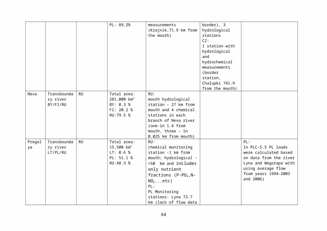
where x is the mean of all values in the time series and SE is the standard error (SE = standard deviation divided by square root of n = number of observations in the time series) and, finally, 1.645 is the 95% percentile in a one sided Gaussian distribution with mean 0 and variance equal 1. A test probability of 5% means that we have a 5% probability of incorrectly rejecting the null hypothesis.
This statistic is called the adjusted mean and if the statistic is less than the target T, then the reduction target is met.
11.7.2. Testing with significant trendsIn the case of a time series of nutrient inputs with a significant trend, another statistical method is needed for testing if a BSAP target is met. Let us assume that the trend is linear, that a linear regression model with year as the independent variable can be fitted to the time series and that estimates for α and β can be calculated – then the linear model can be used to predict a normalized nutrient input for the last year n in the time series. This estimate is calculated as
L̂nN=α̂+ β̂ ∙ year n. (11.11)
Then the standard error of the estimate which is defined as
SEr=√MSE ∙√1/n+ yearn2/∑
i=1
n
yeari2 (11.12)
where MSE is the Mean Squared Error as defined in Chapter 11.5, n is the number of years in the time series, yearn is the last year in the time series (i.e. 2010) and yeari simply stands for a given year in the time series (i.e. 1997). Then calculate the statistic
x AD=L̂nN+ tn−2,0.05 ∙SE r , (11.13)
where t n−2,0.05 is the 95% percentile in a t-distribution with n-2 degrees of freedom (see list below). The mathematical definition of the standard error of the prediction SEr given in (3.5) is a well-known statistic from ordinary linear regression.
Finally, the following “traffic light” system will be used for evaluating whether a country has met the BSAP target, is close to meeting the target or has not met the target. Statistically, the system is defined as:
Red:
If x or L̂nN>T , i.e. the average normalized nutrient input over the considered period or the estimated normalized input for the last year is above target value.
Yellow:
If x∨ L̂nN<T ,and if x AD>T , i.e. the null hypothesis of the target test is accepted, but the average normalized input or the estimated normalized input for the last year is lower than the target.
Green:
If x AD<T , i.e. the null hypothesis of the target test is rejected.
List of 95% percentiles for the one sided t-distribution with n-2 degrees of freedom:
n-2 95% percentile n-2 95% percentile
1 6.314 13 1.7712 2.920 14 1.7613 2.353 15 1.7534 2.132 16 1.746
64

5 2.015 17 1.7346 1.943 18 1.7297 1.895 19 1.7258 1.860 20 1.7219 1.833 21 1.71710 1.812 22 1.71411 1.796 23 1.71112 1.782 24 1.708
The following example applies the methodology. The phosphorus input ceiling for the Kattegat is set to 1,687 tonnes. The normalized total phosphorus inputs also show a significant downward trend, and when applying a linear trend to the time series the normalized input in 2010 is estimated to 1,549 tonnes. This gives the following test value: 1,549+1.761•47=1,634, which is 53 tonnes below the target ( Figure 11.4). Therefore, inputs of phosphorus to the Kattegat are given a green light.
Figure 11.4. Testing the target value for total water and airborne phosphorus inputs to the Kattegat 1995-2010. Black line is target, “------“ line is estimated value in 2010 and “…….” line is test value according to equation 11.13.
11.8. Mathematical description of the Mann-Kendall trend testTrend analysis of a time series of length T consisting of yearly inputs of nutrients can be done by applying Mann-Kendall’s trend test (Hirsch et al. 1982). This test method is also known as Kendall’s τ (Kendall 1975). The aim of this test is to show if a downward or an upward trend over the period of T years is statistically significant or if the time series merely consists of a set of random observations of a certain size. The Mann-Kendall’s trend test has become a very effective and popular method for trend analysis of water quality data.
The Mann-Kendall’s trend test is a non-parametric statistical method, which means that the method has fewer assumptions than a formal parametric test method. The data do not need to follow a Gaussian distribution like in ordinary linear regression, but should be without serial correlation. Furthermore, the method tests for monotonic trends and not necessarily linear trends, and it thus tests for a wider range of possible trend shapes. Monotonic trends are an either downward or upward tendency without any specific
65

form. If the time series data are Gaussian distributed and the trend is actually linear, the power of the Mann-Kendall trend method is slightly lower than that of ordinary linear regression due to the accommodation of the slightly less restrictive assumptions.
Let x1 , x2 ,…, xnbe yearly inputs of total nitrogen or total phosphorus for the years.1,2 ,…, n . The null hypothesis of the trend analysis is that the n yearly data values are randomly ordered. The null hypothesis is tested against the alternative hypothesis that the time series has a monotonic trend. The Kendall statistic is calculated as
S=∑i=1
n−1
∑j=i+1
n
sgn (x j−x i ), (11.14)
where
.
sgn (x )={ 10−1
x>0x=0x<0 .
If either x j or xi is missing then sgn ( x j−x i )=0
per definition.
The trend is tested by calculating the test statistic
.
Z={S−1
(var (S ) )12
0S+1
(var (S ) )12
S>0S=0S<0
.
The variance of S under the hypothesis of no trend is calculated as
var (S )= n (n−1 ) (2n+5 )18 , (11.15)
where n is the number of loads in the time series.
A positive S-value indicates an upward trend and a negative value a downward trend. When both a downward and an upward trend are of interest (a two-sided test), the null hypothesis of randomly ordered
data is rejected when the numerical value of Z is less than the (α
2 ) -percentile or greater than the (1−α
2) -percentile (two-sided test) in the Gaussian distribution with mean value 0 and variance 1. A one-sided test can be carried out as well. The significance level α is typically 5%. The reason for evaluating Z in the standard Gaussian distribution is the fact that S under the null hypothesis is Gaussian distributed with mean
value 0 and variancevar (S ) forn→∞ . The Gaussian approximation is very good if n ≥10 and fair for 5≤n≤10.
An estimate of the trend β (a slope estimate) can be calculated by assuming a constant (linear) trend during the period and presenting the estimate as change per year. Hirsch et al. (1982) introduced Theil-Sen’s slope
estimator: for all pairs of observations (x i , x j ) with calculate
66
nij 1 nij 1 nij 1

d ij=x i−x ji− j . (11.16)
Then the slope estimator is the median value of all the d ij -values and is a robust non-parametric estimator and will generally work for time series with serial correlation and non-Gaussian distributed data. A 100 (1−α )% confidence interval for the slope can be obtained as follows (Gilbert 1987):
Choose the desired confidence level (1, 5 or 10%) and apply
,
Z1−α
2={2 ,576
1 ,9601 ,645
α=0 . 01α=0 . 05α=0 .10 ,
in the following calculations. A confidence level of 5% is standard.
Calculate
Cα=Z1−α2
⋅(var (S ) )12 .
(11.16)
Calculate
M 1=N−Cα
2 , (11.17)
and
M 2=N+Cα
2 , (11.18)
where
N=12n (n−1 ) .
Lower and upper confidence limits are the M 1 th largest and the (M 2+1 ) th largest value of the N ranked
slope estimatesd ij .
A non-parametric estimate for the intercept α can be calculated according to Conover (1980). The estimator is calculated as
α̂=M x− β̂ ∙ M i, (11.19)
where Mx is the median value of all the data in the time series and Mi is the median value of
.
If the time series consists of data from different seasons (i.e. monthly loads), Mann-Kendall’s seasonal trend test may be applied (Hirsch and Slack 1984). This is done by calculating the test statistic S for every season separately. Then the test statistic for the whole time series is equal to the sum of each of the
67
n,,2,1 …
n,,2,1 … n,,2,1 …

seasonal test statistics. We refer to Carstensen and Larsen (2006) for a detailed mathematical description of the seasonal trend test.
68

12. Quality assurance on water chemical analysis
12.1. Specific aspects of quality assurance The Article 3, paragraph 5, of Helsinki Convention states that the Contracting Parties shall ensure that measurements and calculations of emissions from point sources to water and air, and of inputs from diffuse sources to water and air, are carried out in a scientifically appropriate manner in order to assess the state of the marine environment of the Baltic Sea Area and ascertain the implementation of this Convention. Additionally, HELCOM 16 has adopted a quality assurance policy, according to which:
1. Contracting Parties acknowledge that only reliable information can provide the basis for ef fective and economic environmental policy and management regarding the Convention area
2. Contracting Parties acknowledge that environmental information is the product of a chain of activities, constituting programme design, execution, evaluation and reporting, and that each activity has to meet certain quality requirements
3. Contracting Parties agree to quality assurance requirements be set for each of these activities4. Contracting Parties agree to make sure that suitable resources are available nationally (e.g. ships,
laboratories) in order to achieve this goal5. Contracting Parties fully commit themselves to follow the guidelines, protocols etc. adopted by the
Commission and its Committees in accordance with this procedure of quality assurance.
Basic principles of quality assurance are also referred to in the HELCOM Monitoring and Assessment Strategy adopted by the 2013 HELCOM Copenhagen Ministerial Meeting.
Detailed description of general aspects of QA/QC is described in the HELCOM COMBINE Manual, Part B. General Guidelines on Quality Assurance for Monitoring in the Baltic Sea, available on the HELCOM website: HELCOM COMBINE Manual . Technical specifications for chemical analysis and monitoring of water status in relation to the water framework directive can be found in the QA/QC directive (Commission Directive 2009/90/EC) as well.
The Contracting Parties are responsible of the quality assurance of the data submitted to HELCOM PLC-Water database.
The laboratories providing data to PLC should have a quality assurance system that follows the requirements of EN ISO/IEC 17025. Participating laboratories are encouraged to endeavour the obtainment of official accreditation for variables on which they report data in accordance with PLC.
All institutes/laboratories should participate in regular (annual) inter-laboratory comparison tests at relevant levels of nutrients and metals. Also, the laboratories should use appropriate reference materials for internal quality control and assurance. The use of certified reference material is encouraged.
All institutes/laboratories performing the collection of samples to PLC have to be careful in order to get representative and uncontaminated samples. Guidance on sampling can be found in WMO Guidance 168 chapter 7.3 and ISO 5667 standards on Water Quality – Sampling. Different aspects of sampling are covered in different parts of the ISO standard.
All Contracting Parties have to nominate a national QA contact person responsible for PLC quality assurance.
The national QA contact person will help in ensuring comparability and reliability of analytical data provided by the laboratories in their country. The national QA contact person should:
69

provide information about PLC-Water at the national level and guarantee that information on the PLC Guidelines and the QA section of the COMBINE Manual reach the laboratories submitting PLC data
co-operate nationally with the laboratories participating in PLC-Water data collection collect the mandatory information (see end of Chapter 13.4) from laboratories and report them to
PLC-6 Project by the end of October 2015.
The PLC-Water laboratories are asked to estimate the uncertainty of their analytical meas urements. The estimated uncertainties should be reported for the individual variables in the form of expanded measurement uncertainty including a 95% confidence interval together with information on the concentration level. The expanded uncertainty U is obtained by multiplying the combined standard uncertainty Uc by a coverage factor k, which is 2 (rounded values 1.96 from student t-factor) when the level of confidence is 95%:
U=U c ∙2 (12.1)
12.2. Minimum quality assurance by the Contracting PartiesThe COMBINE Manual for marine monitoring in HELCOM describes quality assurance as covering all aspects of analytical investigation, and includes the following principal elements (last updated 26 September 2013):
Knowledge of the purpose of the investigation is essential to establish the required data quality Provision and optimization of appropriate laboratory facilities and analytical equipment Selection and training of staff for the analytical task in question Establishment of definitive directions for appropriate collection, preservation, storage and
transport procedures to maintain the integrity of samples prior to analysis Use of suitable pre-treatment procedures prior to analysis of samples, to prevent uncontrolled
contamination or loss of the determinant in the samples Validation of appropriate analytical methods to ensure that measurements are of the required
quality to meet the needs of the investigations Conduct of regular intra-laboratory checks on the accuracy of routine measurements, by the
analysis of appropriate reference materials, to assess whether the analytical methods are remaining under control, and the documentation and interpretation of the results on control charts
Participation in inter-laboratory quality assessments (proficiency testing schemes, ring-tests, training courses) to provide an independent assessment of the laboratory's capability of producing reliable measurements
The preparation and use of written instructions, laboratory protocols, laboratory journals, etc., so that specific analytical data can be traced to the relevant samples and vice versa.
As minimum quality assurance in PLC, Contracting Parties has to consider:
Monitoring water level and discharge, and establish water level-discharge relationships Guidance on water sampling Demands on sample storage and preservation Demands on laboratory performance Guidance on compiling and assessing data, and reporting data including data on quality assurance.
12.3. Inter-laboratory comparison tests on chemical analysesAll institutes/laboratories should participate in regular (annual) inter-laboratory comparison tests. It is recommended to perform the inter-laboratory comparison tests according to the ISO/IEC Guide 17043. Participation in inter-laboratory comparison tests is obligatory for accredited laboratories as well as for laboratories that have a quality assurance system that follows the requirements of EN/ISO 17025.
70

For the inter-laboratory comparison tests that the laboratories participate in, it is essential that:
the test material is as similar as possible to the matrices (e.g. riverine water and/or wastewater) to be analysed within PLC-Water
different concentration levels of each substance in each matrix are included in the test and they are adequate to the concentrations of the samples collected in PLC-Water
the participating laboratories use the analytical methods, which are intended to apply for PLC-Water.
Inter-laboratory comparison tests can be found in the Internet. Here are some examples:
QUASIMEME: http://www.quasimeme.org
Eurofins: http://www.eurofins.dk/dk/milj0/vores-ydelser/praestationspr0vning-milj0/proficiency-testing-environment.aspx
EPTIS: http://www.eptis.bam.de
Department of Applied Environmental Science, Stockholm University: http://enviropro.itm.su.se
Proftest SYKE, Finnish Environment Institute: http://www.syke.fi/proftest/en
12.4. The PLC-6 inter-laboratory comparison test on chemical analysesAn inter-laboratory comparison test was conducted in 2013 within the PLC6 project in order to have laboratories from each of the CPs participating in the same test study. The aim was to get an overall picture of the quality of the data from chemical analyses and of the comparability of data in PLC.
The inte-rlaboratory comparison study was performed with statistical analysis with outlier test according to ISO/DIS 5725 and Youden plots. The study included nutrients and metals in riverine water and wastewater. In total, 17 laboratories representing all CPs participated with either analyses of nutrients or metals or both in either riverine water and/or wastewater.
In the report on the inter-laboratory comparison test (Lassen & Larsen 2013) it is concluded that:
Generally the analytical quality is good and comparable between the laboratories with a few exceptions, which can at least partly be explained by other factors than the analytical skills
NH4-N showed most likely to be too instable to be included in this kind of inter-comparison test and consequently no conclusions can be made on the analytical performance on this substance
Although the relative total variance between the participating laboratories (CV(R)) on PO 4-P and P-total in riverine water was high, the analytical quality is considered to be acceptable, because the concentration levels were rather low. That implies high CV(R)-values although the absolute variances were low
Mercury concentrations in riverine water showed high deviations. However, it is well known that it is difficult to perform Hg analyses in water with high precision at low concentration levels.
12.5. Validation of PLC-Water chemical dataThe national QA contact persons are responsible for validation of the chemical data to be submitted to the HELCOM PLC-Water Database.
The validation by Contracting Parties of the data should be carried out at the national level based on information on:
71

accreditation status (strongly advised for laboratories) use of quality assurance system that follows the requirements of EN ISO/IEC 17025 (strongly
advised for laboratories) measurement uncertainty, estimated as expanded uncertainty, see Annex 5 (mandatory for
laboratories) limit of quantification (mandatory for laboratories) use of reference material (recommended for laboratories) use of control charts (mandatory for laboratories) participation in laboratory inter-comparison tests (strongly advised for laboratories).
The measurement uncertainty has to be estimated as combined standard uncertainty, which means that reproducibility within laboratory and repeatability between laboratories are included in the calculation of the uncertainty and the further calculation of expanded uncertainty. Examples can be found in Annex 5 and further explanation in Magnusson et al (2004).
Measurement uncertainty can be calculated with a new software tool – Mukit (measurement uncertainty kit), which is based on the Nordtest method [Näykki et al., 2012]. This free software is available in the webpage of the SYKE calibration laboratory (ENVICAL): http://www.syke.fi/envical/en.
Missing mandatory information will be flagged in the PLC-Water database.
12.6. Recommended limits of quantification (LOQ)The levels of quantifications should in principle be lower than the expected concentrations in order to have as few observations as possible below LOQ (to avoid inclusion of concentrations estimated on basis of LOQ in the load calculation). As guidance, the following levels of quantification are suggested not to be exceeded:
Recommended LOQ (should be seen as a guidance level):
Parameter River water WastewaterBOD 0.5 mg l-1
TOC 0.5 mg l-1
NH4-N 10 µg l-1 20 µg l-1
NO23-N 20 µg l-1 40 µg l-1
Ntot 50 µg l-1 200 µg l-1
PO4-P 5 µg l-1 20 µg l-1
Ptot 10 µg l-1 50 µg l-1
Cd 0.01 µg l-1 0.5 µg l-1
Cr 0.05 µg l-1 1.0 µg l-1
Cu 0.1 µg l-1 10 µg l-1
Ni 0.05 µg l-1 1.0 µg l-1
Pb 0.05 µg l-1 1.0 µg l-1
Zn 0.5 µg l-1 5 µg l-1
Hg 0.005 µg l-1 0.5 µg l-1
Comparing the recommended LOQ above with the corresponding LOQ requirements in the Water Framework Directive according to the QA/QC directive (with LOQ ≤ 0.33 • EQS) the HELCOM LOQ recommendations are lower for those metals where it is possible to compare (cadmium, nickel and lead). It must be emphasized that the LOQs in WFD are set in order to determine if the water quality criteria are met, while in PLC they are set in order to obtain as many observations > LOQ as possible in order to estimate the load as precisely as possible.
72
12.7. Values under the limit of quantificationIt is important to distinguish between the limit of detection (LOD – the lowest detectable amount of a compound) and the limit of quantification (LOQ – the lowest quantifiable amount of a compound). Limit of detection (LOD) is the smallest amount or concentration of an analyte in the test sample that can be reliably distinguished from zero. Limit of quantification (LOQ) is a performance characteristic that marks the ability of an analytical method to adequately “quantify” the analyte.
LOQ is in the WFD QA/QC directive (Commission Directive 2009/90/EC) defined as a stated multiple of LOD. There has been much diversity in the way in which LOD of an analytical system is defined. Most approaches are based on multiplication of the within-batch standard deviation of results of blanks by a factor. Further information can be found in the ISO/TS 13530 or in the chapter B.4.2.3. of the HELCOM Combine Manual.
In PLC-6 the LOQ is used to assign a numeric value when handling low-level data. The use of LOQ instead of LOD is in accordance to the EC-directive on quality assurance of water chemical analyses (2009/90/EC).
If measured concentrations are below LOQ, the estimated concentration should be calculated using the equation:
Estimation = ((100%-A) • LOQ)/100, (12.2)
where A=percentage of samples below LOQ11.
12.8. Technical notes on the determination of variables in rivers and wastewaterThis chapter includes technical notes for determination of some variables. For PLC-Water, analysis should be made using unfiltered samples.
The well tested and documented European or international standard methods (EN or ISO) or methods based on these standards are highly recommended to use.
Particles can give rise to light-scattering effects that result in interferences in all photometric nutrient analyses. This bias can be avoided by measuring the sample before addition of the colour reagent, or by filtration or centrifugation where this does not cause contamination.
Particularly in the case of nutrients and metal analysis, a satisfactory blank control is necessary. Therefore, it is important to control the blank daily, for reproducibility and constancy over a longer time. The blank should include all analytical pre-treatment procedures, including the addition of the same quantities of chemical substances as for the samples.
In all analytical work, water of sufficiently high purity shall always be used when needed. High purity water can be distilled or deionized water, “MilliQ-water” or comparable. When very high purity is needed the water might need treatment in several steps, e.g. double or triple distilled water. More information on various degrees of water purity and testing of the purity may be found in ISO 3696:1987.
For calibration purpose in general, a working standard should be prepared from a stock standard solution for every batch of samples.
Apart from manual methods, various automated methods are in use. The analyst has to be aware of the effects of the different analytical conditions in automated analysis that might affect accuracy.
Biological Oxygen Demand (BOD)
11 The QA/QC directive says that when the amount of a measure and is below LOQ the result shall be set to half the value of LOQ in the calculation of annual average values. In PLC it is not annual average values that are calculated but loads, which means that it is two different situations and therefore use of different methods makes sense.
73

For the determination of BOD in wastewater samples it is strongly recommended to follow ISO 5815:2003 “Water quality - Determination of biochemical oxygen demand after n days (BODn) - Part 1: Dilution and seeding method with allylthiourea addition” and in surface water samples “ - Part 2: Method for undiluted samples”.
ISO 5815-1:2003 is applicable to all waters having biochemical oxygen demands greater than or equal to 3 mg/l of oxygen (the limit of quantification) and not exceeding 6 000 mg/l of oxygen.
ISO 5815-2:2003 specifies determination of the biochemical oxygen demand in undiluted samples of water. It is applicable to all waters having biochemical oxygen demands greater than or equal to 0.5 mg/l of oxygen (the limit of quantification) and not exceeding 6 mg/l of oxygen.
BOD should be reported as either BOD5 or BOD7. If BOD is reported as BOD7 it will be stored in the HELCOM PLC-Water database, and for PLC assessments a conversion factor BOD5 = BOD7 /1.15 will be used for converting to BOD5 .
Nutrients
Sample bottles of plastic or glass can be used. It is recommended to use new clean plastic bottles. Every new batch of plastic bottles need to be verified that they are clean by filling them with water of high purity, and after several days analyse the water for potential nutrients. If plastic bottles are reused or if glass bottles are used, they need to be cleaned e.g. by rinsing them in hydrochloric acid (ca 2 mol l -1) and thereafter rinsing them carefully with high purity water. The cleaning procedure has to be verified regularly. The samples should be stored cold (4 C) and dark from sampling until analysis.
Orthophosphate
The molybdenum blue method with reduction by ascorbic acid is recommended for determination of orthophosphate.
The analyses should be carried out as soon as possible. Samples that are not analysed within one day have to be preserved. The samples should be stored cold (4 C) and dark.
Total Phosphorus
Digestion with potassium peroxodisulfate is recommended. For analyses of wastewater with a high content of organic matter a more powerful oxidation method (with nitric-sulfuric acid) may be necessary. A quality control sample can be prepared of e.g. Na--glycerophosphate or thiamine pyrophosphate chloride.
The samples should be stored cold (4 C) and dark, and should be preserved as fast as possible (within one day).
Ammonium
Samples for determination of ammonia should not be preserved. The indophenol blue method is recommended. High concentrations of ammonium can be determined by sample dilution. The Nessler method is not recommended.
The analyses should be carried out as soon as possible and within one day on unpreserved samples. The samples should be stored cold (4 C) and dark.
Nitrate
The cadmium reduction method is recommended for the analyses of nitrate. It is necessary to check the capacity of the reductor (at least 90 % exchange) systematically. The salicylate method is not recommended because of many interfering effects.
74

The analyses should be carried out as soon as possible. Samples that are not analysed within one day have to be preserved. The samples should be stored cold (4 C) and dark.
Total Nitrogen
Total nitrogen in river water can be analysed by a method based on oxidation with potassium per-oxodisulfate followed by reduction of nitrate with a cadmium reductor (cf. Nitrate above). Especially for analyses of industrial wastewater the modified Kjeldahl method with Dewarda´s alloy or the Kjeldahl method and the determination of nitrate separately is recommended. Alternative methods are instrumental methods according to EN 12260:2003, catalytically oxidation of nitrogen in water, in the form of free ammonia, ammonium, nitrite, nitrate and organic compounds capable of conversion to nitrogen oxides under the oxidative conditions. The nitrogen compounds are oxidized to nitrogen oxides, and determined instrumentally by chemiluminiscens (EN 12260:2003).
The quality control sample can be prepared of e.g. EDTA, glycine or 4-nitroaniline.
Metals
The basis for reliable measurements at low metal concentrations in water is to avoid contamination when handling the samples in all the different stages from sampling to the analysis of the samples.
For sampling of riverine water for measurement of metals except mercury (for Hg see below) bottles of polypropylene, polyethene, polytetrafluoroethylene (PTFE) or resistant glass (e.g. Pyrex) are recommended. The bottle and the cap should be prepared from colourless material.
Bottles, glass and plastic ware and containers have to be cleaned by soaking them in nitric acid at least for one day and then be rinsed with water of high purity at least three times. For determination of ultra trace level it is necessary to follow more extensive cleaning procedures. If the laboratory collect both river and wastewater it is necessary to use separate samplers and bottles for sampling at low levels and high levels of metals. It is essential to maintain a clean environment during analyses. All chemicals should be of highest possible purity and high purity water shall be used for preparation of solutions. If low content of metals are to be determined, a field blank shall be analysed as well.
Samples that contain particulate material shall be digested with nitric acid in a closed vessel under pressure.
For measurement of metals, atomic absorption spectroscopy (AAS flame or flameless), inductive plasma-optical emission (ICP-OES) or inductive coupled plasma-mass spectroscopy (ICP-MS) can be used. For measurement of low contents of metals in rivers ICP/MS or anodic stripping voltametry (ASV) are highly recommended.
Calibration is important to carry out correctly. Commercial stock solutions are available for preparation of calibration solutions. The calibration should be performed with a blank solution and 4-5 different calibration solutions for an appropriate concentration range. Need for recalibration has to be checked by measuring a quality control sample once per 20 determinations. In order to reduce potential effects of chemical and physical interferences (i.e. high contents of chlorides) the method of standard addition may be applied. Interference effects can also be reduced by gradual dilution or by addition of different chemical modifiers to the sample. If both high and low contents of metals are determined in the same batch, the high level samples should preferably be analysed after low level samples. If this is not possible there should be a blank sample between the samples in order to prevent the memory effect.
Mercury
Good quality of plastic or resistant glass bottles should be used for collecting of samples for measurement of mercury.
75
The quality of the reagents used for the analyses of mercury should be controlled.
Mercury can be detected with cold vapour atomic absorption or fluorescence spectroscopy. For measurement of low contents of mercury (pg l-1) it is recommended to enrich the mercury on a gold trap before analysis by fluorescence technique.
The control chart on blanks has to be used to enhance the detection of contamination during analyses.
Total Organic Carbon (TOC)
For the determination of TOC in surface and wastewater samples it is strongly recommended to follow the standard ISO 8245:1999 “Water quality -- Guidelines for the determination of total organic carbon (TOC) and dissolved organic carbon (DOC)”, which is identical to EN 1484:1997
Further information on determination on chemical variables is described in Annex B-17 of the HELCOM COMBINE Manual.
76

13. Annual PLC reporting requirementsAccording to HELCOM Recommendation 26/2 “Compilation of Waterborne Pollution Load (PLC-Water)”, the total waterborne inputs to the Baltic Sea should be quantified annually. Hence, every year Contracting Parties should quantify and report the total input to the Baltic Sea from:
Monitored rivers (Chapter 4) Unmonitored areas (Chapter 7), and Point sources (Chapter 5) which discharge directly into the Baltic Sea.
Further, annual transboundary riverine nutrient inputs should be reported for the follow-up on progress in fulfilling the nutrient reduction requirements adopted by the 2013 HELCOM Copenhagen Ministerial Declaration, which has specific nutrient reduction targets for each Contracting Party and assumed reductions in riverine transboundary riverine inputs from non-Contracting Parties and between Contracting Parties (Chapter 8).
The inputs should be reported for each Baltic Sea sub-catchment area (the sub-basin division is described in Chapter 2.6). The parameters to be reported are listed in Chapter 1 (Table 1.1).
Before reporting Contracting Parties should perform quality assurance (Chapter 12) and data validation (Chapter 11). Selected quality parameters should be reported (Chapter 13.4).
All data have to be reported electronically according to the reporting format prepared by the Data Manager (see Annex 2).
13.1. Reporting of the inputs from monitored riversContracting Parties should report the input calculation method(s) and equations applied for quantifying river flow and load. It is recommended to use one of the input calculation methods described in chapters 4 and 5.
Daily flow and daily concentration (interpolated)
Annual input (in kg a-1) calculation based on daily flow and daily concentration regression
An alternative input calculation method (country specific)
If alternative input calculation methods have been used, they need to be described in detail.
The computation of inputs using only annual average of concentration and flow, respectively, is not recom-mended as it leads to uncontrolled large errors. All information and data that have to be reported electronically are summarized in Annex 2.
Table 13.1. Overview of annual reporting obligations related to total inputs from monitored rivers.
REPORTING CATCHMENT CATCHMENT FLOW INPUT
Individually reported by monitored river
Countrysurface area
Annual flow as m³ s-1,Annual min, max as m3 s-1 (voluntary)Long-term average3 (voluntary)
Parameters as in Table 1.1, in t a-1
77

Transboundary1, 2
surface area Annual flow as m³ s-1, Parameters as in Table
1.1, t a-1
Surface water retention of TN and TP on transboundary inputs in the receiving catchment, if updated data/information are available compared to former reported/used data
1 The rivers listed in Table 8.3. The country receiving transboundary inputs is responsible for reporting these inputs. 2 The reporting of inputs from border rivers should be coordinated between the countries sharing the border river.3 The long-term flow should preferably consist of a 30 year period, where 1981-2010 is recommended.
Countries should use their own estimates of retention if specific data about the local conditions are available. Where Contracting Parties do not follow the methods in the guidelines the method should be described, including the calculation methods used, and relevant data and information must be reported (see also Chapter 9).
13.2. Reporting of the input from unmonitored areasThe annual input from unmonitored areas should be reported every year as a total input from the Contract -ing Party to each Baltic Sea sub-basin. Alternatively, the unmonitored part of monitored rivers can be reported individually. Chapter 7 describes methods for estimating inputs from unmonitored areas on the basis of:
model results
land use within these areas, and
extrapolating the knowledge about neighbouring rivers under similar conditions.
The method(s) used to estimate the input from unmonitored areas should be reported. If Contracting Parties use an alternative method, it should be described in detail when reporting.
Diffuse sources discharging directly into the sea must be reported as part of the inputs from unmonitored areas.
All information and data which have to be reported electronically are summarized in Annex 2.
Table 13.2. Overview of annual reporting obligations related to total input from unmonitored areas.
REPORTING CATCHMENT CATCHMENT FLOW INPUTAggregated according to input to marine sub-basin
Surface area Annual flow as m³ s-1 Annual input for parameters listed in Table 1.1, t a-1
13.3. Reporting of the inputs from direct point sourcesContracting Parties are to quantify and report annually the inputs from point sources discharging directly into the Baltic Sea. Point source categories are municipal wastewater treatment plants (MWWTP),
78
industrial plants (INDUSTRY) and aquaculture plants (AQUACULTURE). A description of how to interpret whether an input is direct to the sea is given in Chapter 2.5 and direct (point) sources are defined in Annex 1. Reporting obligations are listed in table 13.3.
Chapter 5 describes how the discharges from point sources are quantified, and these methods should be used when quantifying discharges from point sources entering directly to the Baltic Sea. Contracting Parties are urged to report individually by plant, but it is possible to report aggregated sources by point source category. Quantification of discharges is described in Chapter 5.1 for MWWTP, Chapter 5.2 for INDUSTRY and Chapter 5.3 for AQUACULTURE.
In addition to reporting of inputs from direct point sources, also the methods used for estimating the discharges should also be reported. If Contracting Parties apply any alternative (country specific) method, a detailed description of the calculation method should be reported.
All information and data that have to be reported electronically are summarized in Annex 2.
Table 13.3. Overview of annual reporting obligations related to point sources discharging directly to the Baltic Sea.
INDIVIDUALLY OR AGGREGATED per marine sub-basin1
ANNUAL REPORTINGFLOW LOAD
MWWTP Total, m³ a-1 Annual input for parameters as in Table 1.1, t a-1
Industrial plants Total, m³ a-1 Annual input for parameters as in Table 1.1, t a-1
Aquaculture plants discharging directly to the sea
Total, m³ a-1 (2) Annual input for parameters as in Table 1.1, t a-1
1 Point sources discharging directly to the Baltic Sea should preferably be reported individually, but can be reported as a sum for every Baltic Sea marine sub-basin for municipal effluents, industrial effluents, and aquaculture plants, respectively.(2) Flow does not apply to marine aquaculture plants.
13.4. Reporting on quality assuranceWhen reporting PLC-6 data Contracting Parties should report their quality assurance criteria as:
LOQ Expanded uncertainty Fraction of samples below LOQ
If there are different values for either LOQ or expanded uncertainty for a specific substance, because of more than one laboratory carrying out the monitoring, the most representative values should be reported.
For more information, see Chapter 12 on quality assurance on water chemical analysis.
For modelling, data uncertainty should be reported, see Chapter 13.5.
13.5. Reporting on uncertainty on national data setsContracting Parties should estimate and report on the estimated total uncertainty on their reported data according to Chapter 11.4. The estimated total uncertainty on the total input per sub-catchment should as a minimum be reported. Individual uncertainty categories (see Chapter 11.4) can also be reported.
The uncertainty can be divided in bias (B) and precision (P), where the total uncertainty U is (B2 + P2)0.5.
79

14. Periodic PLC reporting requirementsAccording to HELCOM Recommendation 26/2 “Compilation of Waterborne Pollution Load (PLC-Water)”, in addition to annual quantification of the total waterborne inputs to the Baltic Sea as described in Chapter 13, an assessment of the inputs from different sources within the catchment area of the Baltic Sea located within the borders of the HELCOM Contracting Parties, should be carried out periodically (every six years) starting in 2006.
In such comprehensive waterborne pollution load compilations (assessments), sources of waterborne inputs to inland waters and to the sea should be quantified.
The following should be reported in order to quantify sources of inputs to inland surface waters (the so called source oriented approach):
1. Municipal wastewater treatment plants (Chapter 5.1)
2. Industrial plants (Chapter 5.2)
3. Aquaculture (Chapter 5.3)
4. Nutrient losses from diffuse sources (Chapter 6.2), and
5. Natural background nutrient losses (Chapter 6.1).
In order to quantify the importance of the different sources of waterborne input to the total input entering the Baltic Sea (the so called load-oriented approach), the following information need to be reported in addition to the annually reported inputs from direct point sources and unmonitored areas:
Apportionment of riverine load (Chapter 10), and
Retention (Chapter 9).
The inputs should be reported for each Baltic Sea sub-catchment area (the sub-basin division is described in Chapter 2.6). The parameters to be reported are listed in Chapter 1 (Tables 1.1 and 1.2).
Before reporting Contracting Parties should perform quality assurance (Chapter 12) and data validation (Chapter 11). Selected quality parameters should be reported (Chapter 14.3).
All data have to be reported electronically according to the reporting format prepared by the Data Manager (see Annex 3).
As supporting information, an overview of parameters monitored by Contracting Parties in 2012 was compiled during the PLC-6 project and can be accessed via the PLC-6 project page on the HELCOM website.
Besides the reporting requirement in this chapter, the Contracting Parties must also in year with periodic reporting fulfil the annual reporting requirements in Chapter 13.
Where Contracting Parties do not follow the methods in the guidelines the used method should be described, including the calculation methods used, and all relevant data and information must be reported.
14.1. Source-orientated approach: Methodology for quantifying sources of waterborne inputs to inland waters14.1.1. Data requirementsAccording to the source-oriented approach, the inputs from point sources, diffuse sources and natural background losses into inland surface waters should be quantified. Many different methods are used by the Contracting Parties to estimate inputs from different sources into inland surface water. The following information and data are needed for estimating these inputs:
80

The annual inputs of nitrogen and phosphorus riverine loads (Chapter 4)
The annual point source discharges of nutrients entering inland surface waters upstream the riverine monitoring point(s) (Chapter 5)
Natural background losses to inland surface waters of nitrogen and phosphorus as totals (Chapter 6.1)
Data from the river catchment areas as watershed characteristics: land use; soil types; population (total) connected to sewage systems and population in areas with scattered dwellings (Chapter 2)
Quantification of retention in inland surface waters as rivers, lakes, reservoirs and on inundated floodplains upstream the riverine monitoring point(s), in order to obtain total retention of nitrogen and phosphorus in inland surface waters in the catchment area (Chapter 9)
Any further information on other (potential) sources of diffuse inputs.
Quantifications of the inputs to inland surface waters (Chapter 10).
Tables 14.1-14.8 specify the information to be reported.
Reporting of transboundary inputs in transboundary catchments is described in section 14.1.5.
14.1.2. Point source discharges into inland surface waters and direct discharges from point sources14.1.2.1. MWWTP discharges into inland surface watersDischarges from MWWTPs into inland surface waters within the Baltic Sea catchment area should be reported every six years starting in 2006 and from MWWTP discharging directly to the Baltic Sea every year. Descriptions for measuring flow and calculating input are given in chapters 3.1 and 5, respectively. Annual reporting of MWWTPs discharging directly into the Baltic Sea has been described in Chapter 13.
Discharges from MWWTPs into inland surface waters should be reported as follows:
Monitored river: preferably individually but otherwise aggregated by monitored river Transboundary catchments: preferably individually for the part of the monitored rivers located with
Contracting Parties otherwise aggregated by rivers Unmonitored areas: aggregated by country and sub-basin
All MWWTP > 10,000 PE should preferable be reported individually, although for unmonitored areas they can be reported aggregated. MWWTP < 10,000 PE can alternatively be reported aggregated by monitored river, and for direct discharges by sub-basin.
Flow data, flow measurement methods and estimates of their accuracy should be reported by each Contracting Party. The calculation methodology should be reported. If the inputs based on the annual reporting differs from the inputs included in the periodic reporting every six years (due to different methodology/estimation), both values should be reported in years with periodic reporting.
All information and data that have to be reported are summarized in Annex 3.
Table 14.1. Periodic data reporting on MWWTPs discharging to inland surface water and directly to the Baltic Sea.
MWWTPs DISCHARGING INTO THE INLAND SURFACE WATERS AND DIRECTLY TOTHE BALTIC SEA
REPORTING CATCHMENT LEVEL OF REPORTING FLOW INPUTMonitored rivers reported individually
Individually * Total, m3 a-1 Parameters as in Table 1.2, t a-1
81
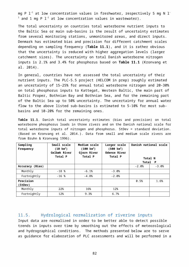
Unmonitored areas aggregated by sub-basin
Individually * Total, m3 a-1 Parameters as in Table 1.2, t a-1
Direct discharges into the Baltic Sea
Individually** Total, m3 a-1 Parameters as in Table 1.2, t a-1
* The flow and inputs should be reported individually for plants >2,000 PE, but can be reported aggregated for plants ≤2,000 PE.
** Russia may report aggregated direct point sources
For all categories mentioned in Table 14.1, also the following information should be reported:
the number of MWWTPs indication of first and second treatment level and elimination of nitrogen and phosphorus )12 ;
additional treatment methods where available; number of connected Population Equivalent (PE) flow data, flow measurement methods and estimation of their accuracy all calculation and estimation methods
14.1.2.2. Discharges of industries into inland surface waters and direct discharges from point sourcesThe quantification of discharges from industrial plants into inland surface waters within the Baltic Sea catchment area should be carried out every six years (starting in 2006) and from industrial plants discharging directly into the Baltic Sea every year (see Chapter 13 for annual reporting). The identification of sources as well as descriptions for measuring flow and calculating input are given in chapters 3.1 and 5, respectively. Minimum reporting of INDUSTRY is linked to the E-PRTR. Plants that have operation permits are subject to self-monitoring and to reporting to the permitting authority. On request, they should provide data to the national PLC data manager. Industrial plants in unmonitored areas can be reported as aggregates by sector described in Annex 6.
Table 14.2. Periodic data reporting on industrial plants discharging into inland surface water and directly to the Baltic Sea.
INDUSTRIAL PLANTS DISCHARGING INTO THE INLAND SURFACE WATERS AND DIRECTLY TO THE BALTIC SEA
REPORTING CATCHMENT
LEVEL OF REPORTING*
FLOW* INPUTS1 No. OF PLANTS
Monitored rivers reported individually
individually Total, m3 a-1 Parameters as in Table 1.2, t a-1
To be reported
Total, m3 a-1 Parameters as in Table 1.2, t a-1
To be reported
Individually/ aggregated
Total, m3 a-1 Parameters as in Table 1.2, t a-1
To be reported
Total, m3 a-1 Parameters as in Table 1.2, t a-1
To be reported
Unmonitored areas
individually Total, m3 a-1 Parameters as in Table 1.2, t a-1
To be reported
12 Russia is clarifying whether they can provide aggregated figures for Russian point sources
82

aggregated by sub-catchment
Total, m3 a-1 Parameters as in Table 1.2, t a-1
To be reported
Individually/ aggregated
Total, m3 a-1 Parameters as in Table 1.2, t a-1
To be reported
Total, m3 a-1 Parameters as in Table 1.2, t a-1
To be reported
Direct discharges into the Baltic Sea (individually by sub-catchment annually)
individually
The same as for annual reporting. Details on reporting obligation are in Chapter 6 and specified in Table 13.3Individually/
aggregated
Reporting of individual industrial plants should include,
the number of industrial plants aggregated; indication of primary, secondary or tertiary treatment level and additional treatment methods
where applicable; flow data, flow measurement methods and estimation of their accuracy;
14.1.2.3. Discharges from aquaculture into inland surface waters and directly to the seaThe quantification of discharges from aquaculture plants into inland surface waters within the Baltic Sea catchment area should be carried out every six years (starting in 2006) and from aquaculture plants discharging directly into the Baltic Sea every year. Descriptions for measuring flow and calculating input are given in chapters 3 and 5.3, respectively.
For PLC-water assessments discharges from aquaculture plants must be reported separately for aquaculture plants with a production > 200 t a-1; but can be reported aggregated for aquaculture plants with a production ≤ 200 t a-1 and for all aquaculture plants in unmonitored areas.
The discharges from aquaculture plants into inland surface waters should be reported:
Monitored river: individually, but may be aggregated for minor aquaculture plants Unmonitored areas: the discharges from aquaculture plants should be reported per Contracting
Party for each Baltic Sea sub-catchment Aquaculture plants discharging directly to the Baltic Sea: reported individually (at least for large
plants), but can be aggregated for minor production units per Baltic Sea sub-basin.
Flow data, flow measurement methods and estimates of their accuracy should be reported by each Contracting Party. The calculation methodology should be reported. If the inputs based on the annual reporting differ from the inputs included in the periodic reporting every six years (due to different methodology/estimation), both values should be reported in years with periodic reporting.
All information and data that have to be reported are summarized in Annex 3.
83

Table 14.3. Periodic data reporting requirements for aquaculture plants and facilities.AQUACULTURE PLANTS DISCHARGING INTO THE INLAND SURFACE WATERS AND DIRECTLY TO THE BALTIC SEA
REPORTING CATCHMENT
SIZE CATEGORY LEVEL OF REPORTING*
FLOW1 LOAD*
Monitored rivers reported individually
Production >200 t a-1 Individually Total, m3 a-1 Parameters as in Table 1.2, t a-1
Production ≤200 t a-1 Individually / aggregated*
Total, m3 a-1 Parameters as in Table 1.2, t a-1
Unmonitored areas aggregated by sub-catchment
Production >200 t a-1 Individually Total, m3 a-1 Parameters as in Table 1.2, t a-1
Production ≤200 t a-1 Individually / aggregated*
Total, m3 a-1 Parameters as in Table 1.2, t a-1
Discharging directly into the Baltic Sea
Production >200 t a-1 Individually Total, m3 a-1 (2) Parameters as in Table 1.2, t a-1
Production ≤200 t a-1 Individually Total, m3 a-1 (2) Parameters as in Table 1.2, t a-1
1 For PLC-water assessments discharges from aquaculture plants must be reported separately for aquaculture plants with a production > 200 t a-1; but may be reported aggregated for aquaculture plants with a production ≤ 200 t a-1 and for all aquaculture plants in unmonitored areas.
(2) For marine aquaculture plants, flow is not to be reported
For all categories mentioned in Table 14.3 that are reported individually, also the following information should be reported:
the number of plants production feed consumption Type of treatment, e.g. no treatment, sediment traps, microsieves, biofilter, plant lagoons and/or
sludge storage (if any) flow data, flow measurement methods and estimation of their accuracy all calculation and/or estimation methods.
84

14.1.3. Diffuse losses to inland surface watersThe quantification of losses from diffuse sources of nutrients into inland surface waters within the Baltic Sea catchment area should be carried out every six years starting in 2006. A description for quantifying losses from diffuse sources is given in Chapter 6.
Table 14.4. Overview of reporting obligations related to losses from diffuse sources of nutrients into inland surface waters
LOSSES FROM DIFFUSE SOURCES INTO INLAND SURFACE WATERS
REPORTING CATCHMENT LOSSESMonitored rivers reported individually Diffuse losses of total N and total P as t a-1 either as a sum of all
delivery pathways or as losses by every individual pathway for: Agriculture as well as managed forestry as a sum or divided
on e.g.: erosion surface runoff interflow tile drainage groundwater
Atmospheric deposition Rainwater constructions and overflows Scattered dwellings
Unmonitored areas1 aggregated by sub-catchment
1 To be reported if source oriented apportionment has been performed on unmonitored areas.
Diffuse losses can also be estimated for every individual pathway (see Figure 2.2). Further it should be stressed that the sum of all pathways for one/more source(s) must give the same figure as the sum of the corresponding source(s).
In the absence of harmonized quantification procedures, the Contracting Parties should apply the most appropriate method/model to quantify losses from diffuse sources taking into account the relevant geology, topography, soil type, climate, land use, and agricultural practices in their region. Applied models must be calibrated with monitoring data and afterwards validated on another set of monitoring data. The Contracting Parties should provide documentation on model validations and calibrations (see Chapter 6.2).
Whatever methodology is adopted by a Contracting Party, it is essential that certain minimum requirements are fulfilled as described in Chapter 6. In particular, the methodology should be based on measurements or upon objectively determined loss coefficients that should be sensitive to variations in losses associated with different land use types (e.g. different agricultural crops, forestry practices and livestock densities).
The nutrient losses from diffuse sources to inland surface waters should be reported in accordance with the requirements of the source-orientated approach:
Monitored river: individually, but may be aggregated for rivers with minor monitored catchment Transboundary areas: individually Unmonitored areas: the losses from diffuse sources of nutrients into inland surface waters should
be reported per Contracting Party for each Baltic Sea sub-catchment.
The applied method should be described in detail and reported. All information and data that have to be reported are summarized in Annex 3.
14.1.4. Natural background losses into inland surface watersThe quantification of natural background nutrient losses to inland surface waters within the Baltic Sea catchment area should be carried out every six years starting in 2006. The losses should be reported in
85
accordance with the requirements in the source-orientated approach, which means every moni tored river shall be reported individually, whereas aggregated data may be reported for rivers with minor monitored catchment. A description of the quantification of inputs from natural background losses is given in Chapter 6.1.
For unmonitored areas the natural background nutrient losses to inland surface waters should be reported per Contracting Party to each Baltic Sea sub-catchment. The applied method should be described in detail and reported.
All information and data that have to be reported are summarized in Annex 3.
Table 14.5. Overview of reporting obligations related to natural background losses into inland surface waters.
NATURAL BACKGROUND LOSSES INTO INLAND SURFACE WATERS
REPORTING CATCHMENT EVERY SIX YEAR REPORTINGMonitored rivers reported individually Total N and total P, t a-1
Unmonitored areas1 by sub-catchment Total N and total P, t a-1
1 To be reported if source oriented apportionment has been performed on unmonitored areas.
14.1.5. Transboundary inputsFor transboundary river catchments transboundary inputs should be reported as a source “transboundary inputs” when determining the source apportionment for monitored or unmonitored catchments. The Contracting Party receiving transboundary input also have the possibility to carry out and report source apportionment on the transboundary inputs (dividing in inputs from point sources (MWWTP, industry, aquaculture), diffuse losses to inland waters and natural background losses).
Table 14.6. Overview of reporting of transboundary inputs
REPORTING CATCHMENT EVERY SIX YEAR REPORTING
Transboundary river catchments individually2
Total N and total P, t a-1
Countries receiving transboundary inputs from an upstream country can report the transboundary input as the source” transboundary inputs” or alternatively can carry out source apportionment on these inputs.
14.1.6. Retention of nutrientsRetention calculations should be carried out every six years starting in 2006. For unmonitored areas, retention estimates should be reported per Contracting Party for each Baltic Sea sub-catchment. The applied estimation method should be reported together with retention figures. The Contracting Party may report retention for different source categories if possible, but this is voluntary. Methods for calculating retention are described in Chapter 9.
The retention should be reported as follows:
Monitored river: individually, but may be aggregated for rivers with minor monitored catchment Transboundary areas: individually per river Unmonitored areas: aggregated by Contracting Party for each Baltic Sea sub-catchment.
All information and data which have to be reported electronically are summarized in Annex 3.
86

Table 14.7. Overview of periodic reporting obligations on nutrient retention.RETENTION
REPORTING CATCHMENT Total average retention in catchment*
Retention in tonnes per year of gross load
Monitored rivers Individually per river N and P in t a-1 t a-1
Transboundary area Individually per river N and P in t a-1 t a-1
Unmonitored areas Aggregated by sub-catchment N and P in t a-1 t a-1
A written report, describing the characteristics of the catchment areas, such as catchment size, run-off, area of surface waters and the estimates of the quantified retentions, should be enclosed with the periodic reporting. The methods used and the results should also be reported for transparency. Since the nutrient retention rate may vary considerably during a year, the retention should be reported as a yearly or longer than yearly average.
14.2. Load-oriented approach - reporting riverine load apportionmentFor periodic assessments, the importance of different sources (point, diffuse and natural background losses) contributing to the total nutrient inputs entering into the Baltic Sea sub-basins also has to be assessed (riverine load assessment). This requires the quantification of inputs from different sources in:
Monitored rivers (transboundary parts separately when relevant) Unmonitored areas Direct point sources (reported annually)
For periodic assessments, the importance of different sources (point, diffuse and natural background losses) contributing to riverine nutrient load has also to be assessed, taking into account retention in inland surface waters which requires the quantification of:
Retention in inland surface waters and Riverine load apportionment.
The assessment of riverine inputs by source at the river mouth is further described in Chapter 10.2.
Riverine load apportionment should be carried out every six years starting in 2006. The following information should be preferably reported individually for the monitored part of the catchment area of every monitored river or aggregated for some of the monitored rivers with minor (monitored) catchment. For unmonitored areas the riverine load apportionment figures should be reported per Contracting Party for each Baltic Sea sub-catchment.
The following information should be reported:
Annual point source discharges, losses from diffuse sources and natural background losses, for nitrogen and phosphorus as total and as percentage (see Chapters 5 and 6);
Annual retention for nitrogen and phosphorus (river-internal retention and retention in lakes (see Chapter 9); and
Description of the methods used for the riverine load apportionment and for the retention (see chapters 9 and 10).
87

The diffuse source inputs to the Baltic Sea should be assigned to sources as follows:
Agriculture Managed forestry Atmospheric deposition (to surface water) Natural background input Scattered dwellings Storm water and overflow (if not connected to MWTTP)
Point source discharges to the Baltic Sea should be divided into the following categories:
Wastewater treatment plants (MWWTP) Industrial units (Industrial plant) Aquaculture (Aquaculture plants)
The applied estimation methods should be reported together with riverine load apportionment data. All information and data that have to be reported are summarized in Annex 3.
Table 14.8. Overview of periodic reporting obligations related to riverine nutrient load apportionment.
RIVERINE LOAD APPORTIONMENTREPORTING CATCHMENT Natural background
sourcesAnthropogenic sources
Point sources1 Diffuse sources2
Monitored rivers3
Individually Total N and P, t a-1 and as % of the total
Total N and total P, t a-1
by point source category1
Total N and total P, t a-1 by diffuse source category
Unmonitored areas3
Aggregated by sub-basin
Total N and P, t a-1 and as % of the total
Total N and total P, t a-1
by point source category1
Total N and total P, t a-1 by diffuse source category
1 MWWTP, industrial plants, aquaculture plants and other point sources.2 If methods exist, diffuse sources can be further divided into pathways, but this is voluntary (as specified in Chapter 6).3 Transboundary inputs at the border should be reported (see Table 8.3)
14.3. Reporting on uncertainty on national data setsContracting Parties should estimate and report on the estimated total uncertainty on their reported data according to Chapter 11.4. The estimated total uncertainty on the total input per sub-catchment on reported data according to Chapter 14 should be estimates and reported as a minimum. Individual uncertainty categories (see Chapter 11.4) can also be reported.
The uncertainty can be divided in bias (B) and precision (P), where the total uncertainty U is (B2 + P2)0.5.
88

15. ReferencesBehrendt, H. 1996. Inventories of point and diffuse sources and estimated nutrient loads - a comparison for different river basins in central Europe. Water, Science and Technology, 33, 4-5, 99-107.
Behrendt, H. 1999. A comparison of different methods of source apportionment of nutrients to river basins . Water, Science and Technology, 39, 12, 179-187.
Behrendt, H. & Opitz, D. 1999. Retention of nutrients in river systems: Dependence on specific run-off and hydraulic load. Hydrobiologia, 410, 111-122.
Behrendt, H., Dannowski, R., Deumlich, D., Dolezal, F., Kajewski, I., Kornmilch, M., Korol, R., Mioduszewski, W., Opitz, D., Steidl, J. & Stronska, M. 2003. Point and diffuse emissions of pollutants, their retention in the river system of the Odra and scenario calculations on possible changes. Weissensee Verlag, Berlin, 296 p.
Behrendt, H., Bach, M., Kunkel, R., Opitz, D., Pagenkopf, W.-G., Scholz, G. & Wendland, F. 2003. Quantifizierung der Nährstoffeinträge der Flussgebiete Deutschlands auf der Grundlage eines harmonisierten Vorgehens. UBA/Texte 82/03, 194 p.
Billen, G., Garnier, J., Billen, C. & Hannon, E. 1995. Global change in nutrient transfer from land to sea: biogeochemical processes in river systems. GMMA, Free University of Brussels, 99 p.
Cardone, M. 1986a. New technique in chemical assay calculations. 1. A survey of calculation practices on a model problem. Analytical Chemistry, 58: 433438.
Cardone, M. 1986b. New technique in chemical assay calculations. 2. Correct solution of the model problem and related concepts. Analytical Chemistry, 58: 438445.
Carstensen, J. & Larsen, S. E. 2006. Statistisk bearbejdning af overvågningsdata – Trendanalyser. NOVANA. (Statistical assessment of monitoring data. Trend analysis. NOVANA). Danmarks Miljøundersøgelser. 38 s. – Teknisk anvisning fra DMU nr. 24. http://www.dmu.dk/Pub/TA24.pdf (in Danish).
Cho, C.Y., Hynes, J.D. Wood, K.R. & Yoshida H.K. 1991. Quantitation of fish culture wastes by biological (nutritional) and chemical (limnological) methods; the development of high nutrient dense (HND) diets. In: Cowey, C.B. & Cho, C.Y. (eds). Nutritional strategies and aquaculture waste. Proceedings of the First International Symposium on Nutritional Strategies in Management of Aquaculture Waste. University of Guelph, Ontario. pp 37–50.
Conover, W.J. 1980. Practical Nonparametric Statistics. Second Edition. John Wiley and Sons, New York.
Ekholm, P., Kronvang, B., Posch, M. & Rekolainen, S. 1995. Accuracy and precision of annual nutrient load estimates in Nordic rivers. National Board of Waters and the Environment. Vesi- ja ympäristöhallinnon julkaisuja - sarja A, no. 205.
EC 1991. Council Directive of 21 May 1991 concerning urban waste water treatment (91/271/EEC), UWWTD. Official Journal of the European Communities, No. L 135/40, 30 May 1991.
EC 2000. Directive 2000/60/EC of the European Parliament and of the Council (QA/QC directive). Technical Specifications for chemical analysis and monitoring of water status. 21 July 2009.
EC 2009. Directive 2009/90/EC on the technical specifications for chemical analysis and monitoring of water status came into force on 20 August 2009. It is a 'daughter' Directive of the Water Framework Directive (2000/60/EC) (WFD) and is commonly known as the QAQC (Quality Assurance Quality Control) Directive.
EC 2010. Directive 2010/75/EU of the European Parliament and of the Council of 24 November 2010 on industrial emissions (integrated pollution prevention and control) (Recast).
89
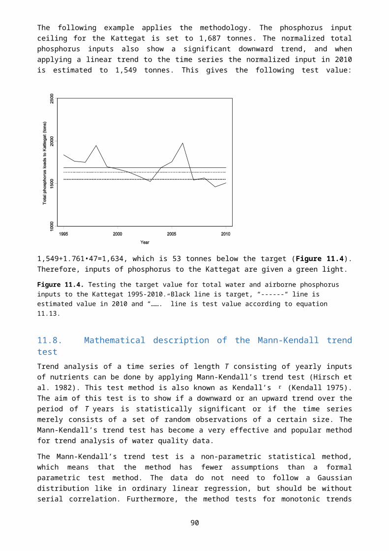
EN ISO/IEC 2005. General requirements for the competence of testing and calibration laboratories. EN ISO/IEC 17025.
EN 1997. Water analysis - Guidelines for the determination of total organic carbon (TOC) and dissolved organic carbon (DOC). EN 1484
EN 12260 2003. IDT Water quality - Determination of nitrogen - Determination of bound nitrogen, following oxidation to nitrogen oxides.Gilbert, R.O. 1987. Statistical Methods for Environmental Pollution Monitoring. New York: Van Nostrand Reinhold.
Gorsuch, T. 1970. The destruction of organic matter. Pergamon Press, Oxford.
Grimvall, A. & Stålnacke, P. 1996. Statistical methods for source apportionment of riverine loads of pollutants. Environmetrics 7: 201-213.
Gustafsson, B.G & Mörth, C.M. (in prep.). Revision of the Maximum Allowable Inputs and Country Allocation Scheme of the Baltic Sea Action Plan V. 3 with contributions from the BNI team: Müller-Karulis, B., Gustafsson, E., Hong, B., Humborg, C. Lyon, S. Nekoro, M., Rodriguez-Medina, M., Savchuk, O., Smedberg, E., Sokolov, A., Swaney, D. & Wulff, F. Baltic Nest Institute, Stockholm University, SE-106 91 Stockholm.
Harmel, R. D., Smith, D. R., King, K. W. & Slade, R. M. 2009. Estimating storm discharge and water quality data uncertainty: A software tool for monitoring and modeling application. Environmental Modelling & Software, 24, 832-842.
HELCOM 1994a. Environment Committee (EC). Report of the 5th Meeting, Nyköping, Sweden, 1014 October 1994. EC5/17, Annex 9.
HELCOM 1994b. Environment Committee (EC). Report of the 5th Meeting, Nyköping, Sweden, 1014 October 1994. EC 5/17, Annex 8.
HELCOM COMBINE Manual, Part B. General Guidelines on Quality Assurance for Monitoring in the Baltic Sea. http://helcom.fi/action-areas/monitoring-and-assessment/manuals-and-guidelines/combine-manual
HELCOM 2004. HELCOM Recommendation 25/4 “Measures aimed at the reduction of discharges from fresh water and marine fish farming”. Adopted 2 March 2004. Supersedes HELCOM Recommendations 18/3 and 20/1.
HELCOM 2005. HELCOM Recommendation 26/2 “Compilation of Waterborne Pollution Load (PLC-Water)”. Adopted 2 March 2005. Supersedes HELCOM Recommendations 15/2 and 19/4.
HELCOM 2007. Baltic Sea Action Plan. Adopted 15 November 2007 in Krakow, Poland.
HELCOM 2011. The Fifth Baltic Sea Pollution Load Compilation (PLC-5). Helsinki Commission – Baltic Marine Environment Commission, Helsinki. Baltic Sea Environment Proceedings No. 128.
HELCOM 2013. HELCOM Copenhagen Declaration "Taking Further Action to Implement the Baltic Sea Action Plan - Reaching Good Environmental Status for a healthy Baltic Sea". Adopted 3 October 2013.
HELCOM in prep. Updated Fifth Baltic Sea Pollution Load Compilation. Final report of the PLC-5.5 project.
Hejzlar, J., Anthony, S., Arheimer, B., Behrendt, H., Bouraoui, F., Grizetti, F., Groenendijk, P., Jeuken, M.H.J.L., Johnsson, H., Lo Porto, A., Kronvang, B., Panagopoulos, Y., Siderius, C., Silgram, M., Venohr, M. & Zaloudík, J. 2009. Nitrogen and phosphorus retention in surface waters: an inter-comparison of predictions by catchment models of different complexity. J. Environ. Monit., 2009, 11, 584-593
Herschy, R.W. 2009. Streamflow measurements. Third edition, Routledge Taylor & Francis, 507 p.
90

Hirsch, R.M. & Slack, J.R. 1984. A nonparametric trend test for seasonal data with serial dependence. Water Resources Research, 20, 727-732.
Hirsch, R.M., Slack, J.R. & Smith, R. A. 1982. Techniques of trend analysis for monthly water quality data. Water Resources Research, 18, 107-121.
Hong, B., Swaney, D.P., Mörth, C.-M., Smedberg, E., Hägg, H.E., Humborg, C., Howarth, R.W., & Bouraoui, F. 2012. Evaluating regional variation of net anthropogenic nitrogen and phosphorus inputs (NANI/NAPI), major drivers, nutrient retention pattern and management implications in the multinational areas of Baltic Sea basin. Ecological Modelling 227, 117–135.
Howarth, R.W., Billen, G., Swaney, D., Townsend, A., Jaworski, N., Lajtha, K., Downing, J.A., Elmgren, R., Caraco, N., Jordan, T., Berendse, F., Freney, J., Kudeyarov, V., Murdoch, P. & Zhao-Liang, Z. 1996. Regional nitrogen budgets and riverine N & P fluxes for the drainage’s to the North Atlantic Ocean: Natural and human influences. Biogeochemistry, 35: 75-139.
Integrated Pollution Prevention and Control (IPPC). Reference Document on the General Principles of Monitoring. November 2002
ISO/IEC 1996. Proficiency testing by interlaboratory comparisons – Part 1: Development and operation of proficiency testing schemes. ISO/IEC Guide 43-1.
ISO 2004. Water quality - Determination of adsorbable organically bound halogens (AOX). ISO 9562.
ISO 2003. Water quality - Determination of biochemical oxygen demand after n days (BODn). ISO 5815.
ISO 2000. Water quality - Determination of hydrocarbon oil index - Part 2: Method using solvent extraction and gas chromatography. ISO 9377-2.
ISO 1999. Water quality -- Guidelines for the determination of total organic carbon (TOC) and dissolved organic carbon (DOC). ISO 8245.
ISO/TS 13530 2009. Water quality - Guidance on analytical quality control for chemical and physicochemical water analysis.
ISO 17025 2005. General requirements.
ISO 5667-2 Water quality – Sampling. Part 2: Guidance on sampling techniques.
ISO 5667-3 Water quality – Sampling. Part 3: Guidance on the preservation and handling of water samples.
ISO 5667-6 Water quality – Sampling. Part 6: Guidance on sampling of rivers and streams.
ISO 5667-9 Water quality – Sampling. Part 9: Guidance on sampling from marine waters.
ISO 5667-10 Water quality – Sampling. Part 10: Guidance on sampling of waste waters.
ISO 5667-14 Water quality – Sampling. Part 14: Guidance on quality assurance of environmental water sampling and handling.
Jensen, J.P., Jeppesen, E., Bøgestrand, J., Pedersen, A.R., Søndergaard, M., Windolf, J. & Sortkjær, L. 1994. Ferske vandområder - søer. Vandmiljøplanens Overvågningsprogram 1993. Danmarks Miljøundersøgelser. 94 s. - Faglig rapport fra DMU nr. 121. 94 pp. [in Danish]
Jensen, J.P., Pedersen, A.R., Jeppesen, E. & Søndergaard, M. 2006. An empirical model describing the seasonal dynamics of phosphorus in 16 shallow eutrophic lakes after external loading reduction. Limnol. Oceanogr., 51(1, part 2), 2006, 791–800. http://aslo.net/lo/toc/vol_51/issue_1_part_2/0791.pdf.
Kelly, C.A., Rudd, J.W.M., Hesslein, R.H., Schindler, D.W., Dillon, P.J., Driscoll, C.T., Gherini, S.A. & Hecky, R.E. 1987. Prediction of biological acid neutralisation in acid sensitive lakes. Biogeochemistry, 3: 129-141.
91
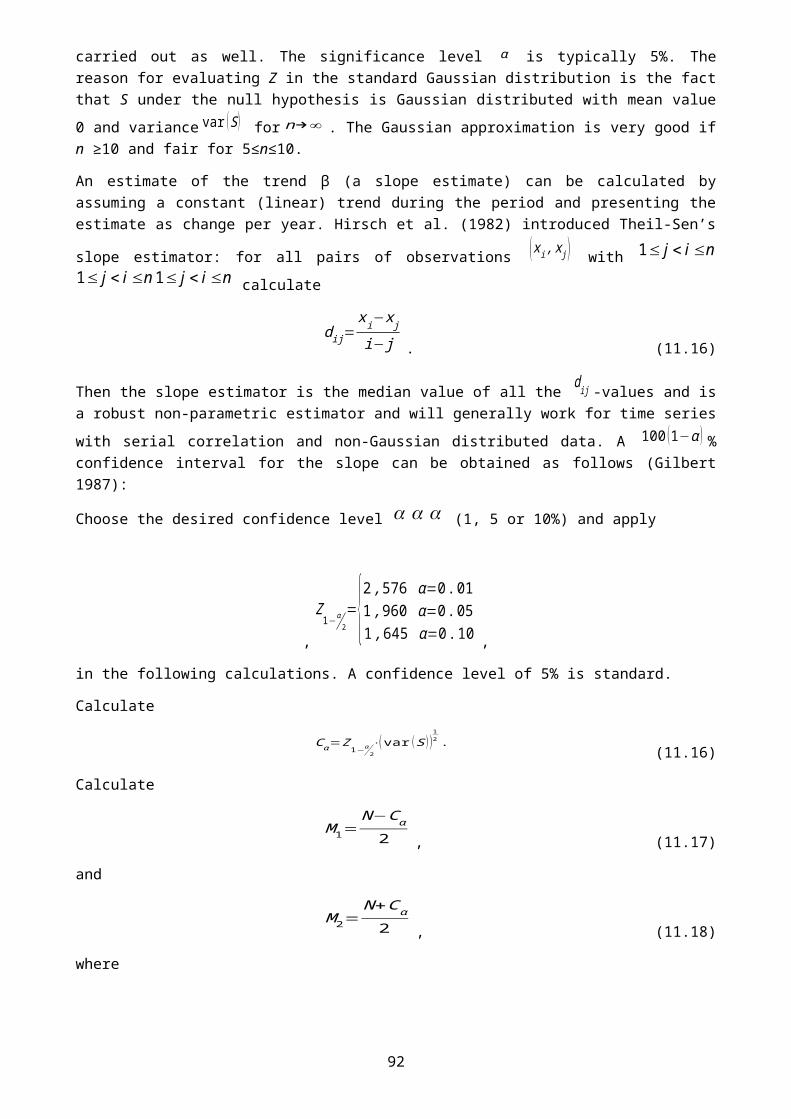
Kendall, M.G. 1975. Rank Correlation Methods. Charles Griffin, London.
Kronvang, B. & Bruhn, A. 1996. Choice of sampling strategy and estimation method for calculating nitrogen and phosphorus transport in small lowland streams. Hydrological Processes 10: 1483-1501.
Kronvang, B., Behrendt, H., Andersen, H.E., Arheimer, B., Barr, A., Borgvang, B., Bouraoui, F., Granlund, K., Grizetti, Groenendijk, P., Schwaiger, Hejzlar, J., E., F., Hoffmann, L., Johnsson, H., Panagopoulos, Y., Porto, A. Lo, Reisser, H., Schoumans, O.F., Anthony, S., Silgram, M., Venohr, M. & Larsen, S.E., 2009: Ensemble modelling of nutrient load in 17 European catchments. J. Environ. Monit., 2009, 11, 572-583.
Kronvang, B., Larsen, S.E., Windolf, J. & Søndergaard, M. 2014. Uncertainties in monitoring – how much do we tolerate. Presentation of NJF Workshop, 19-21 March 2014, Stavanger, Norway.
Lassen, P. & Larsen, M.M. 2013. Report on the HELCOM PLC6 intercalibration. Aarhus University, DCE – Danish Centre for Environment and Energy, 138 pp. Technical Report from DCE – Danish Centre for Environment and Energy No. 27.
Magnusson, B., Näykki, T., Hovind, H., & Krysell, M. 2004. Handbook for calculation of measurement uncertainty in environmental laboratories, 2nd edition. NORDTEST Report TR 537. http://www.nordicinnovation.net/nordtestfiler/tec537.pdf
Näykki, T., Virtanen, A. & Leito, I. 2012. Software support for the Nordtest method of measurement uncertainty evaluation. Accred. Qual. Assur. 17:603-612. http://www.springerlink.com/content/704121770l181786/.
OSPAR 2004. OSPAR HARP NUT Guideline 2: Guidelines for the Quantification nd Reproting if Noitrogen and Phosphorus Discharges/Losses from Aquaculture Plants.
OSPAR 2007. OSPAR HARP NUT Guideline 6: Guideline for the Quantification and Reporting of Nitrogen and Phosphorus Losses from from Diffuse Anthropogenic Sources, and natural Background Losses.
Rekolainen S., Pitkänen H., Bleeker A. & Felix S. 1995. Nitrogen and phosphorus fluxes from Finnish agricultural areas to the Baltic Sea. Nord. Hydrol. 26: 55-72.
Rönnback, P., Sonesten L. & Wallin M. 2009. Transport of substances during spring flow in rivers Ume älv and Kalix älv (Ämnestransporter under vårflöden i Ume älv och Kalix älv). Swedish University of Agricultural Sciences, Department of Aquatic Sciences and Assessment, Report 2009:20 (In Swedish with an English summary).
Schoumans, O.F. & Silgram, M. 2003. Review and literature evaluation of nutrient quantification tools. EUROHARP report 1-2003, NIVA report SNO 4739-2003, Oslo, Norway 2003. Available from http://rapp.niva.no/symfoni/RappArkiv4.nsf/URL/C125730900460902C1256FB800545652/$FILE/4739-2003_72dpi.pdf.
Schoumans, O.F., Silgram, M., Groenendijk, P., Bouraoui, F., Andersen, H.E., Kronvang, B., Behrendt, H., Arheimer, B., Johnsson, H., Panagopoulos, Y., Mimikou, M., Reisser, H., LeGall, G., Barr, A. & Anthony, S.G. 2009a. Description of nine nutrient loss models: capabilities and suitability based on their characteristics. J. Environ. Monit., 2009, 11, 506-514.
Schoumans, O., Silgram, M., Walvoort, D.J.J., Groenendijk, P., Bouraoui, F., Andersen, H.E., Lo Porto, A., Reisser, H., LeGall, G., Anthony, S., Arheimer, B., Johnsson, H., Panagopoulos, Y., Mimikou, M., Zweybert, U., Behrendt, H. & Barr, A. 2009b. Evaluation of the difference of eight model applications to assess diffuse annual nutrient losses from agricultural land. J. Environ. Monit., 2009, 11, 540-533.
Schreiber, H., Behrendt, H., Constantinescu, L., Cvitanic, I., Drumea, D., Jabucar, D., Juran, S., Pataki, B., Snishko, S. & Zessner, M. 2003. Harmonised Inventory of point and diffuse Emissions of Nitrogen and Phosphorus in the Danube Basin. Final Report, Institute of Freshwater Ecology and Inland Fisheries, Berlin, 158 S.
92

SGQAC Meeting 2004, Helsinki. WP 7.4.
Silgram, M. Schoumans, O.F., Walvoort, D.J., Anthony, S.G., Groenendijk, P., Stromqvist, J., Bouraoui, F., Arheimer, B., Kapetanaki, M., Lo Porto, A. & Mårtensson, K. 2009. Subannual models for catchment management: evaluation model performance on three European catchments. J. Environ. Monit., 2009, 11, 526-539.
Stålnacke, P., Grimvall, A., Libiseller, C., Laznik, A. & Kokorite, I. 2003. Trends in nutrient concentrations in Latvian rivers and the response to the dramatic change in agriculture. Journal of Hydrology 283: 184–205.
Svendsen, L.M., Behrendt, H., Knuuttila, S. & Salo, S. 1995. Guideline to estimate natural and anthropogenic contributions to riverine fluxes (source apportionment). TC-POLO 3/7 1995. Ad Hoc Expert Group on pollution Load to the Baltic Sea. Report of Third Meeting, Riga, Latvia, 5-8 June 1995, Helsinki Commission, Baltic Marine Environment Protection Commission, Annex 5.
Svendsen, L.M., Kronvang, B., Kristensen, P. & Græsbøl, P. 1995. Dynamics of phosphorus compounds in a lowland river system: importance of retention and non-point sources. Hydrological Processes 9: 119-142.
Vink, R. & Behrendt, H. 2002. Emissions, immissions and retention processes of heavy metals in the Rhine and Elbe drainage areas and their tributaries. Hydrological processes, 16, 3227-3244.
Vollenweider, R. 1975. Input-Output Models with Special Reference to the Phosphorus Loading Concept in Limnology. Schweiz. Z. Hydrolo 37:53-83.
Vollenweider, R.A. & Kerekes, J. 1982. Eutrophication of waters - Monitoring, assess ment and control. Synthesis Report, OECD Paris, 154 pp.
Windolf, J., Jeppesen, E., Jensen, J.P. & Kristensen, P. 1996. Modelling of seasonal variation in nitrogen retention: a four-year mass balance study in 16 shallow lakes. - Biogeochemistry 33: 25-44.
WMO 2008. Guidance to Hydrological Practices. Volume 1. Hydrology – From Measurement to Hydrological Information. World Meteorological Organization, WMO No. 168 Sixth ed. 2008. WNT, Warszawa, p. 296.
93
Annex 1.List of definitions and acronyms
Airborne Substances carried or distributed by air.Anthropogenic Caused by human activities.Aquaculture The cultivation of aquatic animals and plants, in natural or controlled
marine or freshwater environments.Atmospheric deposition Airborne nutrients or other chemical substances originating from
emissions to the air and deposited from the air on land and water surfaces.
Border river A river that has its outlet to the Baltic Sea at the border between two countries. For these rivers, the loads to the Baltic Sea are divided between the countries in relation to each country’s share of total load.
BAP Baltic ProperBAS The entire Baltic Sea (as a sum of the Baltic Sea sub-basins). See the
definition of sub-basins.BNI Baltic Nest Institute, Stockholm University, Sweden.BOB Bothnian BayBOS Bothnian SeaBSAP Baltic Sea Action PlanBY BelarusCalculated value A value determined by mathematical calculation as opposed to a value
derived from monitoring.Catchment area The area of land bounded by watersheds draining into a body of water
(river, basin, reservoir, sea).Contracting Parties Signatories of the Helsinki Convention (Denmark, Estonia, European
Commission, Finland, Germany, Latvia, Lithuania, Poland, Russia and Sweden).
Country-Allocated Reduction Targets (CARTs)
Country-wise requirements to reduce waterborne and airborne nutrient inputs to reach the maximum allowable nutrient input levels (MAI) in accordance to the Baltic Sea Action Plan.
DCE Danish Center for the Environment and Energy, Aarhus University, Denmark.
DE GermanyDiffuse sources Sources without distinct points of emission e.g. agricultural and forest
land, natural background sources, scattered dwellings, atmospheric deposition (mainly in rural areas)
Direct (point) sources Point sources (municipal wastewater treatment plants (MWWTP), industrial plants and aquaculture plants) discharging (defined by location of the outlet) directly to the sea.
DK DenmarkDS Danish StraitsEE EstoniaEMEP Cooperative Programme for Monitoring and Evaluation of the Long-range
Transmission of Air Pollutants in EuropeEPER European Pollutant Emission RegisterEstimated value A number that has been calculated approximately (the amount, extent,
magnitude, position, or value of something). A tentative evaluation or rough calculation, which accepts that there is uncertainty in the values.
94

Eutrophication Condition in an aquatic ecosystem where increased nutrient concentrations stimulate excessive primary production, which leads to an imbalanced function of the ecosystem.
FI FinlandFlow normalization A statistical method that adjusts a data time series by removing the
influence of variations imposed by river flow, e.g. to facilitate assessment of development in e.g. nitrogen or phosphorus inputs without being obstructed by variations in water flow.
GUF Gulf of FinlandGUR Gulf of Riga
Input ceiling The allowable amount of nitrogen and phosphorus input per country and sub-basin. It is calculated by subtracting the CARTs from the input of nitrogen and phosphorus during the reference period of the BSAP (1997-2003).
KAT Kattegat
HELCOM PRESSURE HELCOM Working Group on Reduction of Pressures from the Baltic Sea Catchment Area
LT LithuaniaLV LatviaMaximum Allowable Input (MAI)
The maximum annual amount of a substance that a Baltic Sea sub-basin may receive and still fulfill HELCOM’s ecological objectives for a Baltic Sea unaffected by Eutrophication.
Measured value An amount determined by measurement.
Monitored areas The catchment area upstream of the river monitoring station. The chemical monitoring decides the monitored area in cases where the locations of chemical and hydrological monitoring stations do not coincide.
Monitoring stations Stations where hydrographic and/or chemical parameters are monitored.MWWTP Municipal wastewater treatment plantNon-contracting parties Countries that are not partners to the Helsinki Convention 1992, but that
have an indirect effect on the Baltic Sea by contributing with inputs of nutrients or other substances via water and/or air.
PL Poland
PLC Pollution Load CompilationPoint sources Municipal wastewater treatment plants (MWWTP), industrial plants and
aquaculture plants that discharge (defined by location of the outlet) into monitored areas, unmonitored areas or directly to the sea (coastal or transitional waters) through one or several outlets.
QA Quality assuranceReference period The BSAP reference period is 1997-2003Reference input The average normalized water + airborne input of nitrogen and
phosphorus during the reference period 1997-2003 used to calculate CARTs and input ceilings.
Retention The amount of a substance lost/retained during transport in soil and/or water including groundwater from the source to a recipient water body. Generally, retention is only related to inland surface waters in these guidelines.
Riverine inputs The amount of a substance carried to the maritime area by a watercourse (natural or man-made) per unit of time.
RU Russia
Statistically significant In statistics, a result is called "statistically significant" if it is unlikely to
95

have occurred by chance. The degree of significance is expressed by the probability, P. P< 0.05 means that the probability for a result to occur by chance is less than 5%.
Sub-basins Sub-division units of the Baltic Sea: the Kattegat (KAT), The Sound (SOU), Western Baltic (WEB), Baltic Proper (BAP), Gulf of Riga (GUR), Gulf of Finland (GUF), Archipelago Sea (ARC) Bothnian Sea (BOS) and Bothnian Bay (BOB). The whole Baltic Sea is abbreviated BAS. Cf. Figure 2.5
SE Sweden
Transboundary input Transport of an amount of a substance (via air or water) across a country border.
TN and TP Total nitrogen and total phosphorus, which includes all fractions of nitrogen and phosphorus.
Unmonitored area Any sub-catchment(s) located downstream of the (riverine) chemical monitoring point within the catchment and further all unmonitored catchments; e.g. unmonitored part of monitored.
Waterborne Substances carried or distributed by water.WFD EU Water Framework DirectiveWMO World Meteorological Organization
96

Annex 2.Annual reporting formats
As agreed earlier the Contracting Parties will annually collect data on river inputs, inputs of unmonitored areas and direct point sources to the Baltic Sea.
The collected data will be used for
develop and update core pressure indicators;
assessment of the progress of Maximum allowable Inputs (MAI);
Core pressure indicator on nutrient inputs;
develop and update Country Allocation Reduction Targets (CART); and
other products used by Contracting Parties, scientific community, media, etc.
The modernization of the PLC database and the structural changes has been completed. In order to make the data more available a Web Application has been established for the data base. The data can be accessed via the Application and it also serves for downloading and uploading the data.
The annual data will be reported by using a reporting template. The reporting template can be down loaded as prefilled. Once filled in, the template should be saved and uploaded to the Application.
Before the actual annual reporting background information on rivers, sub-catchments, stations and point sources should be revised and submitted before 31 August of the following year. The revised background information can be reported by using the previous year’s annual template.
Annual data should be submitted before 31 October of the following year after the sampling, i.e. 2014 data should be delivered before 31 October 2015.
Instructions include reporting templates. They have been established separately for each Contracting Party as CC_ANNUAL_REPORTING_yyyy.XLSX (CC standing for COUNTRY_CODE, e.g. DE = GERMANY, DK = DENMARK, EE = ESTONIA, FI = FINLAND, LV = LATVIA, LT = LITHUANIA, PL = POLAND, RU = RUSSIA and SE = SWEDEN).
For example for Denmark the file is: DK_ ANNUAL_REPORTING_ yyyy.XLSX. (yyyy = reporting year)
Reporting in general
During the data entry following the listed instructions would ease the reporting and increase probability of successful uploading, but also diminish the error messages/warnings of the upload report.
No additional columns should be inserted or any prefilled rows, columns shouldn’t be deleted in the prefilled spreadsheets
Decimal separator to be used '.' (dot) not a ',' (comma)
If the type of an attribute is ‘NOT NULL’ , data must be reported.
Each reported attribute heading has a comment box (Table 1), which consists of a format of the data and a list of options and/or instructions for data entry. Any of the boxes can be made visible by moving the mouse to the heading.
Many of the cells also include an instruction box or a drop-down menu for entering the data, but they also may include constraints and may even show an error message, when trying to enter data in an incorrect
97
format. Instructions will be displayed as drop down menu (Table 2) and the constraints will block false data entry and error messages will give further advice.
The aim is to improve the quality of the entered data and to ease the final QA process. The constraints work only for the punched data. ‘Copy – Paste’ -commands in the templates will remove the defined constraints.
When entering any data the length and the type of format must be respected, e.g., (CHAR (9)) = 9 characters SCDK00001, (CHAR (7)) = 7 characters MDE0005, Date (10) dd.mm.yyyy as should be 01.01.2014. Period name format is (STRING 4-10) like 01-07-2014 (day), 07-2014 (month) or 2014 (year).
Fixed length of characters has been noted as e.g., ‘CHAR (9)’, a variable length of characters either as ‘STRING (1-255)’, ‘CHAR (4)’ and small numbers as ‘(INTERGER)’. In case of number with decimal the length and the number of decimals have been noted as (DECIMAL (8.2)) (=nnnnn.nn).
Reporting obligations will be indicated in each of the spreadsheet of the template as follows:
= ‘Prefilled data’ i.e. tentative definitions of existing in the database once established will be indicated in gray color in the template
= Mandatory information - data will be indicated in pink in the template, e.g. sub-catchment and point source codes in load flow tables, parameters, parameter types, values, value units, etc.
= Voluntarily reported information - data will be indicated in white in the template, e.g. national codes, links, sector codes, etc.
Table 1. An example of a comment box
98

Table 2. An example of a drop-down menu.
At this stage the load / flow reporting will be carried out on an annual basis, but in the future also more detailed reporting might take place. Then total loads, average flows and concentrations could be reported on a monthly, or even on a daily basis. Table 3 gives an overview of the reporting, i.e., source, type of source and a reference where to report data.
Table 3. An overview of the annual data reporting.
SOURCE REPORTING AREAL AND POINT SOURCE INFORMATION FLOW REPORTING LOAD REPORTING
RIVER or MONITORED CATCHMENT
INDIVIDUALMON_RIVER_BACKGROUND
- MON_RIVER_LOAD
UNMONITORED SUBCATCHMENT (by PARAMETER)
BY SUBBASIN and PARAMETER
UNMON_SUBCATCHMENT_BACKGROUND UNMON_SUBCATCHMENT_BACKGROUND
TRANSBOUNDARYSUBCATCHMENT INDIVIDUAL
TRANSB_SUBCATCHMENT_BACKGROUNDTRANSBOUNDARY_FLOW_LOAD
TRANSBOUNDARYSUBCATCHMENT INDIVIDUAL
TRANSB_SUBCATCHMENT_BACKGROUNDTRANSB_SUBCATCHMENT_RETENTION
MONITORED STATION of RIVER INDIVIDUAL
STATION_BACKGROUNDSTATION_FLOW_CONCENT-RATION -
POINT SOURCES of 3 CATEGORIES
INDIVIDUAL POINT SOURCE_BACKGROUND MUNICIPAL_FLOW_LOADINDUSTRIAL_FLOW_LOADAQUACULTURE_LOAD
AQUACULTURE PRODUCTION INDIVIDUAL
AQUACULTURE_PRODUCTION- -
Background information
The annual data reporting includes collection of background information on different sources, i.e. areal definitions, stations and point sources.
The sources are: Monitored sub-catchments, river catchments, unmonitored areas (by parameter), transboundary sub-catchments (country wise), hydrological and chemical stations and individual point sources in three different categories (MWWTP, Industry and Aquaculture).
99

In the MON RIVER_BACKGROUND sheet will be listed
monitored sub-catchments within one country (code example SC+cc+nnnnn)
monitored transboundary rivers (code example RC+cc + nnnnn); and
monitored border rivers (code example RC+cc + nnnnn)
Transboundary and border rivers will be listed in the template of the Contracting Party who has the reporting responsibility of the river, i.e., The CP which has the lowest monitoring station of the river has the reporting responsibility if not agreed differently. Both the transboundary and border rivers have a slightly different catchment code compared with the sub-catchments (RCccnnnnn instead of SCccnnnnn). Figure 1 at the end of the annex clarifies the difference between a sub-catchment and a river catchment and the background information to be reported.
For example, for the entire river (RCLV00055) DAUGAVA the following sub-catchments should be listed:
SCLV00055 (only the Latvian part), SCBY00001, SCRU00049, SCLT00009 and SCEE00035, as listed in table 4. In the sheet the attribute ‘IS_PRIMARY_STATION’ indicates the catchment, which includes the lowest monitoring station.
Additional information to be collected from rivers and separate sub-catchments are: river mouth coordinates, as latitude and longitude (in WGS-84), national sub-catchment and river code, monitoring status (IS_MONITORED), and surface and lake areas (in km2).
Transboundary catchments will be divided to sub-catchments by country (TRANS_SUBCATCHMENT _BACKGROUND).
Table 4. An example for transboundary sub-catchments
All unmonitored sub-catchment information of a country will be listed in the UNMONITORED SUBCATCHMENT BACKGROUND sheet. In case an unmonitored area varies by parameter, each unmonitored area (in km2) and parameter should be listed individually as in table 5.
Table 5. An example of unmonitored sub-catchments
100

The ‘station’ and ‘point source’ information in STATION_BACKGROUND and in POINT_SOURCE_BACKGROUND –sheets to be collected are:
code of a station or a point source and their activity status (‘IS_ACTIVE’ and ‘REPORTING_END_DATE’);
location, i.e., coordinates of each monitoring station or an outlet of an individual point source (in decimal degrees, (WGS-84) latitude and longitude),
related sub-catchment (of each station) recipient sea area (for a discharging point source) and size (in km2) of the monitored area of each station
In addition, information on national station code, EU national point source code and E- PRTR sector type can be reported.
Reference sheet for each set of background information has been indicated in table 6 and the type and the format of all the reported background information are listed by attribute and by spreadsheet in table 7 and 8.
Once the definitions and background information by country have been updated in the database, a tentative list of information will be prefilled by the application when annual reporting templates are downloaded.
The prefilled information of areal definitions, stations or point sources to be reported will be updated before the actual reporting (agreed deadline on 31 of August each year). Once the prefilled information have been provided, none of the data sets, i.e. monitored rivers or sub-catchments, unmonitored areas, transboundary catchments or point sources should be deleted. For rivers and sub-catchments the attribute ‘IS_MONITORED’ indicates whether the catchment has been reported or not in that year, and similarly for stations ‘IS_ACTIVE’ attribute indicates if the station has been reported or not.
101

Table 6. Background information to be reported.GENERAL VIEW OF THE ANNUAL BACKGROUND INFORMATION TO BE PROVIDED
BACKGROUND DEFINITIONS
REPORTINGREFERENCE TABLE
SURFACE AREAS ADDITIONAL INFORMATIONTOTAL_
DRAINAGE (in km2)
COUNTRY_DRAINAGE(in km2)
CONTROL AREA by STATION (in km2)
TRANSBOUNDARY DRAINAGE (in km2)
RIVER/MONITORED CATCHMENTannually
INDIVIDUAL
MON_RIVER_BACKGROUND
X X X
River mouth coordinates;IS_MONITORED /IS_ UNMONITORED during the period; end date of the catchment validity: lake area of the catchment
UNMONITORED SUBCATCHMENT and PARAMETERannually
BY SUBBASIN and PARAMETER
UNMON_SUBCATCHMENT_BACKGROUND
X
Lake area of the catchment
TRANSBOUNDARYSUBCATCHMENTannually
INDIVIDUALTRANSB_SUBCATCHMENT_BACKGROUND
X X X
Lake area of the catchment
MONITORED STATION annually INDIVIDUAL STATION_BACKGRO
UNDX
activity/station coordinates
POINT SOURCES of 3 CATEGORIES annually
INDIVIDUAL POINT SOURCE_BACKGROUND
outlet coordinates; PRTR_sector code;end date of a PS (date of closing)
Table 7. Data type and format of catchment background information
ATTRIBUTE/SHEET MON_RIVER_BACKGROUND
UNMON_SUBCATCHMENT_BACKGROUND_
TRANS_SUBCATCHMENT_BACKGROUND
SUBCATCHMENT_CODE CHAR (9) CHAR (9) CHAR (9)SUBCATCHMENT_NAME STRING (1-255) STRING (1-255) STRING (1-255)SUBCATCHMENT_TYPE CHAR(1) CHAR(1)RIVER_CATCHMENT_CODE CHAR(8) - CHAR(8)PARAMETER_ID - INTEGER -RIVER_MOUTH_LATITUDE DECIMAL (dd.dddd) - -RIVER_MOUTH_LONGITUDE DECIMAL (dd.dddd) - -RIVER_TYPE CHAR(1) - CHAR(1)NATIONAL_SUBCATCHMENT_CODE STRING (1-255) - STRING(1-255)NATIONAL_RIVER_CODE STRING (1-255) - STRING(1-255)NR_CATCHMENTS INTEGER INTEGER INTEGERIS_MONITORED INTEGER - INTEGERPERIOD_NAME STRING (4-10) STRING (4-10) STRING (4-10)IS_PRIMARY_STATION - - BIT 0/1CREATION_DATE DATE(10) dd.mm.yyyy DATE(10) dd.mm.yyyy DATE(10) dd.mm.yyyyEND_DATE DATE(10) dd.mm.yyyy DATE(10) dd.mm.yyyy DATE(10) dd.mm.yyyyTOTAL_DRAINAGE_AREA DECIMAL (8.2) DECIMAL (8.2)UNMONITORED_AREA - DECIMAL (8.2) -
COUNTRY_DRAINAGE_AREA DECIMAL (8.2) - DECIMAL (8.2)TRANSBOUNDARY_AREA - - DECIMAL (8.2)LAKE_AREA DECIMAL (8.2) DECIMAL (8.2) DECIMAL (8.2)
REMARKS STRING(1-255) STRING(1-255) STRING(1-255)
102

Table 8. Data type and format of station and point source background information
ATTRIBUTE/SHEET STATION_BACKGROUND POINT_SOURCE_BACKGROUND
STATION_CODE CHAR (7) -SUBCATCHMENT_CODE CHAR (9) CHAR (9)SUBCATCHMENT_NAME STRING (1-255) STRING (1-255)STATION_NAME STRING (1-25) -PLANT_CODE - STRING (7)PLANT_NAME - STRING (1-255)PERIOD_NAME STRING (4-10) STRING (4-10)IS_ACTIVE BIT 0/1 -RIVER_CATCHMENT_CODE CHAR(8) -NATIONAL_STATION_CODE STRING (1-25) -EU/NATIONAL_CODE - CHAR(255)PRTR_SECTOR_CODE *) - CHAR(1)STATION/PLANT_CODE_LAT DECIMAL (dd.dddd) DECIMAL (dd.dddd)STATION/PLANT_CODE_LON DECIMAL (dd.dddd) DECIMAL (dd.dddd)WFD_CODE STRING (1-50) -REPORTING_START_DATE - DATE(10)REPORTING_END_DATE - DATE(10)TOTAL_NR_OF_PLANTS - INTEGER
TOTAL_NR_OF_TREATED_PLANTS - INTEGERMONITORED_AREA DECIMAL (8.2) -REMARKS STRING(1-255) STRING(1-255)
*) The document listing new PRTR_SECTOR_CODEs can be downloaded: http://prtr.ec.europa.eu/docs/Summary_activities.pdf
Data collection
Loads of monitored sub-catchments and transboundary rivers should be reported individually and for unmonitored areas as aggregated by basin and country. The loads of unmonitored sub-catchments can specifically and optionally be reported for each parameter separately. Then also the respective surface areas should be reported for each unmonitored area and parameter.
Loads and flows of MONITORED RIVERs
The loads of monitored rivers should be reported in the MON_RIVER_LOAD sheet. The following loads should be reported:
loads of monitored rivers within one country loads of transboundary rivers loads of border rivers
The collected mandatory and voluntary parameters have been listed in the PLC-6 Guidelines (Table 1.1)
In some cases the conducted measurements are below the LOQ / LOD (Limit of quantification / detection). LOQ/LOD information (LIMIT_VALUE, LIMIT_UNIT NR_BELOW_LIMIT) should be reported in the MON_RIVER_LOAD sheet. Related to LOQ/LOD information, also the number of measurements and total uncertainty for the obtained load should be reported.
Total flow of a monitored river should be reported in the STATION_FLOW_CONCENTRATION sheet by monitoring station.
The collected mandatory and voluntary parameters have been listed in the PLC-6 Guidelines (Table 1.1)
Flow will be reported as m3/s and the other parameters as t a-1 or kg a-1 (heavy metals).
As for the background information, the reporting responsibility of a transboundary/border river is for the country which has the lowest monitoring station of the catchment
103
to report the total inputs
to report transboundary input at the border
Reporting of loads will be agreed between the countries sharing a transboundary river. Figure 1 at the end of the document clarifies the reporting of sub-catchment and transboundary loads.
The loads and flows of separate catchments (by country, i.e. country allocations) of transboundary and border rivers should be reported in the TRANSBOUNDARY_FLOW_LOAD sheet. Related to the transboundary loads their retention can be reported on a voluntary basis in the TRANB_SUBCATCHMENT_RETENTION
Reported parameters are: average flow, Ntot and Ptot and they will be reported as m3 s-1 and in t a-1 or kga-1.
Additional information on total uncertainty and basic calculation information should be reported. Reporting of LOQ/LOD information should be reported for monitored transboundary loads, as well.
Loads and flows of UNMONITORED AREAs
The data for unmonitored area should be reported by country and by basin. Each unmonitored area consists of the areas between the monitored catchments, unmonitored parts of the monitored rivers, coastal areas and islands. Both the loads and flow of unmonitored areas should be reported in the UNMON_SUBCATCHMENT_ FLOW_LOAD sheet.
The loads and flow of each unmonitored area should also include all loads and flow for the point sources in the area.
The reported parameters for unmonitored areas have been listed in table 1.1. Flow will be reported as m3 s-
1 and the other parameters as t a-1 or kg a-1. Total uncertainty of obtained loads should be reported. Calculation methodology can also be reported.
An overview of the reported data has been presented in table 9 and type and format of loads, flow and metadata by attribute and for each spreadsheet have been compiled in table 10.
104
Table 9. An overview of the data for the annual reportingGENERAL VIEW OF THE ANNUAL DATA REPORTING ON SUBCATCHMENTS AND STATIONS
SOURCE REPORTING REFERENCE TABLE FLOW LOAD ADDITIONAL INFORMATION
CALC. ESTIMATION METHODS
MONITOREDRIVERs annually INDIVIDUALLY MON_RIVER_LOAD as listed in
Table 1.1
LOQ/LOD information, total uncertainty
X
TRANDBOUNDARY/BORDERRIVERs annually
ENTIRE RIVER MON_RIVER_LOAD as listed in Table 1.1
LOQ/LOD information, total uncertainty
UNMONITORED SUBCATCHMENT annually(*
BY COUNTRY AND BASIN, (OPTIONALLY BY PARAMETER)
UNMON_SUBCATCHMENT_FLOW_LOAD
average flow (in m3 s-1)
as listed in Table 1.1 Total uncertainty X
TRANSBOUNDARYSUBCATCHMENTannually(**
INDIVIDUALLY for each SUBCATCHMENT
TRANSBOUNDARY_FLOW_LOAD
average flow (in m3 s-1)
as listed in Table 1.1 X
TRANSBOUNDARYSUBCATCHMENTannually(***
INDIVIDUALLY for each TRANSBOUNDARY SUBCATCHMENT
TRANSBOUNDARY_:RETENTION
as listed in Table 1.1
MONITORED STATION annually INDIVIDUALLY STATION_FLOW_
CONCENTRATIONaverage flow (in m3 s-1) (****
Annual min, max and long-term flows (1981-2010) and concentrations voluntarily (m3/s, µg/l or mg/l)
X
(* Unmonitored parts of monitored rivers should be reported together with unmonitored areas(** Transboundary loads/flow of monitored rivers only Flow, Ntot and Ptot should be reported on a mandatory basis(*** Retention of the nutrient load of transboundary sub-catchments can be reported on a voluntary basis(**** Voluntarily minimum, maximum and long-term flows can be reported
Table 10. Type and format of sub-catchment (load and flow) and station (flow and concentration) data
ATTRIBUTE/SHEET MON_RIVER_LOAD UNMON_SUBCATCHMENT_FLOW_LOAD
TRANSBOUNDARY_FLOW_LOAD
TRANSBOUNDARY_RETENTION
STATION_FLOW_CONCENTRATION
STATION_CODE - - - CHAR (7)SUBCATCHMENT_CODE CHAR (9) CHAR (9) CHAR (9) CHAR (9) CHAR (9)SUBCATCHMENT_NAME STRING (1-255) STRING (1-255) STRING (1-255) STRING (1-255) STRING (1-255)PARAMETER_ID INTEGER INTEGER INTEGER INTEGER INTEGERPARAMETER_TYPE CHAR (3) CHAR (3) CHAR (3) CHAR (3) CHAR (3)PERIOD_NAME STRING(4-10) STRING(4-10) STRING(4-10) STRING(4-10) STRING(4-10)PERIOD_TYPE CHAR (1) CHAR (1) - CHAR (1)IS_LOQ/LOD BIT (0/1) - BIT (0/1) -LIMIT_VALUE DECIMAL (8(.6)) - DECIMAL (8(.6)) -LIMIT_UNIT CHAR(4) - CHAR(4) -NUMBER_BELOW_LIMIT INTEGER - INTEGER -NR_MEASUREMENTS INTEGER - INTEGER INTEGERVALUE DECIMAL (10(.3)) DECIMAL (10(.3)) DECIMAL (10(.3)) DECIMAL (10(.3)) DECIMAL (10(.3))VALUE_UNIT STRING(3-6) STRING(3-6) STRING(3-6) STRING(3-6) STRING(3-6)TOT_UNCERTAINTY INTEGER INTEGER INTEGER INTEGER INTEGERDATA_SOURCE_FLAG CHAR(2) CHAR(2) CHAR(2) CHAR(2) CHAR(2)METHOD_ID INTEGER INTEGER INTEGER INTEGER INTEGERREMARKS STRING(1-255) STRING(1-255) STRING(1-255) STRING(1-255) STRING(1-255)
Loads and flows of DIRECT POINT SOURCEs
Annual loads and flows of direct point sources will be reported individually and for three different categories, municipal wastewater treatment plants (MWWTP), industries and aquaculture. Direct point source has been defined in chapter 2.5 and in Annex 1 as: “Direct point sources: Point sources discharging
105
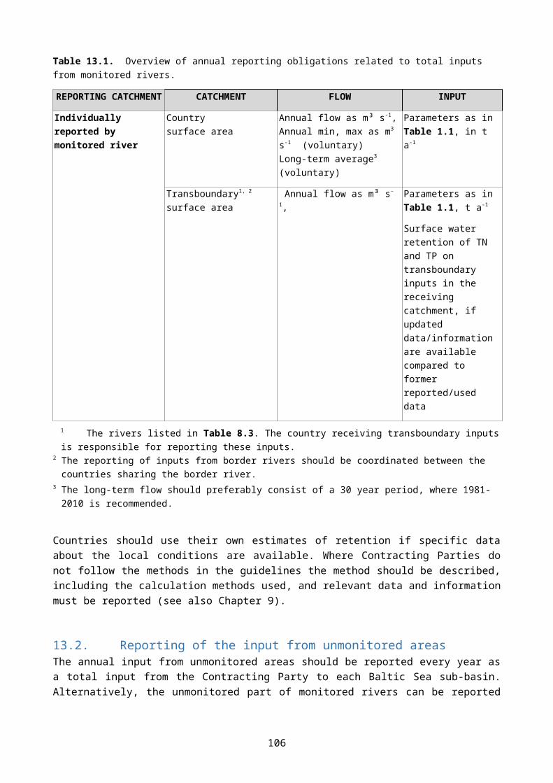
(defined by location of the outlet) directly to the sea”. Further, this implies, that the loads and flow data of point sources, which are located downstream the monitoring station, but not discharging directly to the sea, should be included in the loads of unmonitored areas.
The data to be reported by different category have been listed below (table 11).
MWWTPs
The data to be collected on municipal wastewater treatment plants have been listed in the table 1.1.
Flow will be reported as total flow in m3 a-1 and the other parameters as t a-1 or kg a-1.
Information on LOQ or LOD (IS_LOQ/LOD) and related data, number of measurements (NR_MEASUREMENTS) and total uncertainty (TOT_UNCERTAINTY) are mandatory to report. Information on sampling methodology, and used methods can be reported voluntarily.
INDUSTRIES
The data to be collected on industrial plants have been listed in the table 1.1
Flow will be reported as total in m3 a-1 and the other parameters as ta-1 or kg a-1. Information on LOQ or LOD (IS_LOQ/LOD) and related data, number of measurements (NR_MEASUREMENTS) and total uncertainty (TOT_UNCERTAINTY) are mandatory to report. Information on sampling methodology, and used methods can be reported voluntarily.
AQUACULTURAL PLANTS
The parameters to be collected on aquacultural plants have been listed in the table 1.1
Flow will be reported as total in m3 a-1 and Ntot, Ptot or BOD5/7 as t a-1 or as kg a-1. Total uncertainty of the obtained loads should be reported and used methods on a voluntary basis, respectively.
Apart from the load reporting, amount of feed, feed type and fish production can be reported on a voluntary basis in the AQUACULTURE_PRODUCTION -sheet
The type and format of point source load flow and metadata as well as the information on aquacultural production have been presented in Table 12.
106
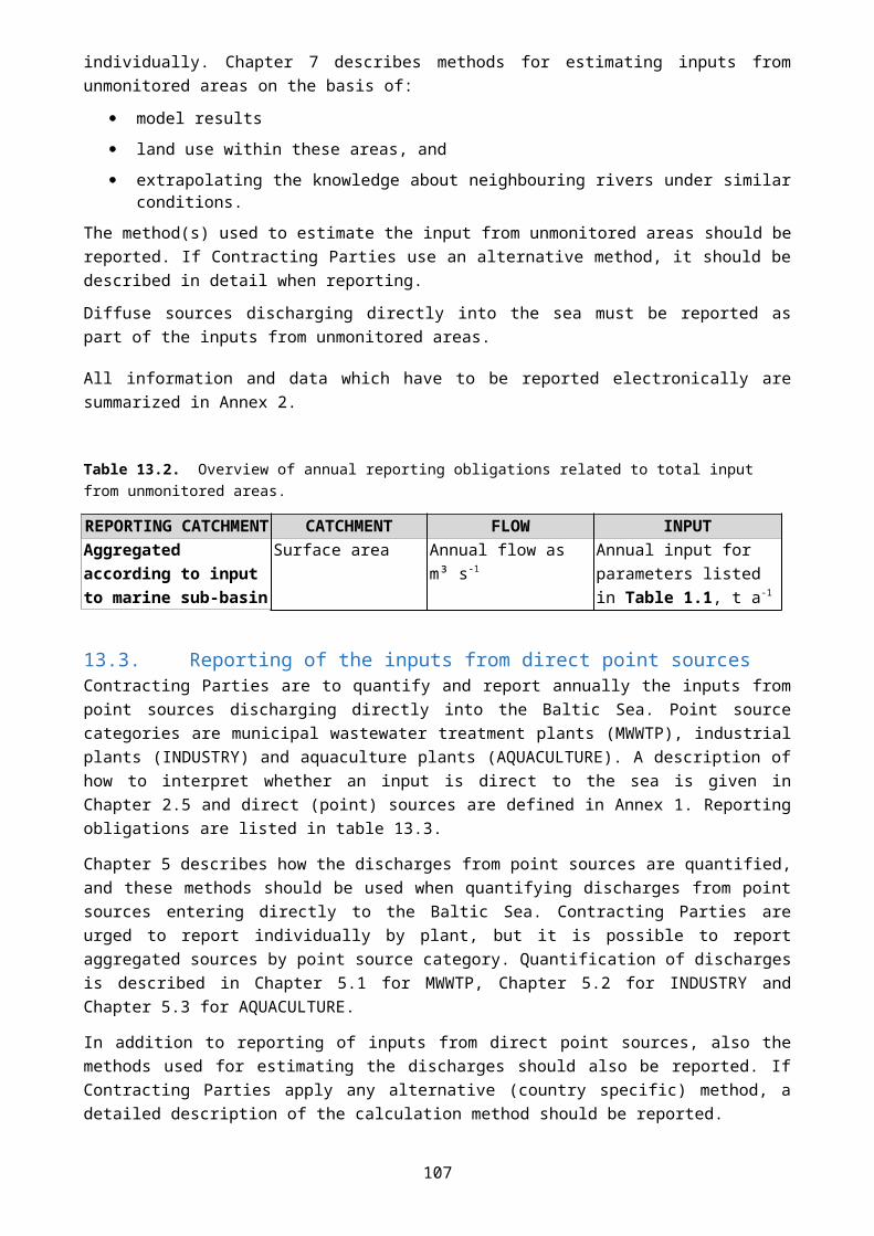
Table 11. An overview of the point source data for annual reportingGENERAL VIEW OF THE ANNUAL DATA REPORTING ON POINT SOURCES
SOURCE REPORTING REFERENCE TABLE FLOW LOAD ADDITIONAL INFORMATION
CALC. ESTIMATION METHODS OF INPUTS
MWWTPannually
MWWTPsINDIVIDUALLY(*
MUNICIPAL_LOAD_FLOW m3 a-1 as listed in
Table 1.1
LOQ/LOD and related information, total uncertainty
X
INDUSTRYannually
INDUSTRIES INDIVIDUALLY (*
INDUSTRIAL_LOAD_FLOW m3 a-1 as listed in
Table 1.1
LOQ/LOD and related information, total uncertaintyPRTR sector/ individual reporting
X
AQUACULTURE annually
AQUACULTURE INDIVIDUALLY(* AQUACULTURE_LOAD m3 a-1 (**
as listed in Table 1.1 Total uncertainty X
AQUACULTURE annually
AQUACULTURE INDIVIDUALLY(*
AQUACULTURE_PRODUCTION
Voluntarily feed type, amount of feed used and total production
(* Russian point sources will partly be reported as aggregated (** Flow of an individual aquaculture can be reported on a voluntary basis when it is relevant, i.e. outlet of discharges exists.
Table 12. Type and format by attribute and spreadsheet of the point source data
ATTRIBUTE/SHEET MUNICIPAL_LOAD_FLOW
INDUSTRIAL_LOAD_FLOW
AQUACULTURE_LOAD
AQUACULTURE_PRODUCTION
PLANT_CODE CHAR (7) CHAR (7) CHAR (7) CHAR (7)SUBCATCHMENT_CODE CHAR (9) CHAR (9) CHAR (9) -SUBCATCHMENT_NAME STRING (1-255) STRING (1-255) STRING (1-255) -PARAMETER_ID INTEGER INTEGER INTEGERPARAMETER_TYPE CHAR (3) CHAR (3) CHAR (3)PERIOD_NAME STRING (4-10) STRING (4-10) STRING (4-10) STRING (4-10)PERIOD_TYPE CHAR (1) CHAR (1) CHAR (1) -IS_LOQ/LOD BIT 1/0 BIT 1/0 - -LIMIT_VALUE DECIMAL (8(.6)) DECIMAL (8(.6)) - -LIMIT_UNIT CHAR(4) CHAR(4) - -NUMBER_BELOW_LIMIT INTEGER INTEGER - -NR_MEASUREMENTS INTEGER INTEGER - -VALUE DECIMAL (10(.3)) DECIMAL (10(.3)) DECIMAL (10(.3)) -VALUE_UNIT STRING(3-6) STRING(3-6) STRING(3-6) -TOT_UNCERTAINTY INTEGER INTEGER INTEGER -SAMPLING_METHODOLOGY CHAR(1) CHAR(1) - -DATA_SOURCE_FLAG CHAR(2) CHAR(2) CHAR(2) -METHOD_ID INTEGER INTEGER INTEGER -
FEED_TYPE - - - CHAR(1)AMOUNT_OF_FEED - - - DECIMAL (10(.3))AQUACULTURE_PRODUCTION - - - DECIMAL (10(.3))
REMARKS STRING(1-255) STRING(1-255) STRING(1-255) -
107

Figure 1. Reporting river catchment and monitored sub-catchment background information and flow and loads.
108

Annex 3.Periodic reporting formats
These will be included in the guidelines after they have been finalized in autumn 2014 – pending on-going work under the PLUS project
109

Annex 4.Example of instructions to personnel carrying out the sampling
Note: Collection of water samples in rivers can potentially be dangerous and CPs should therefore ensure that safety instructions are given. Some countries have legislative requirements for the safety of personnel.
Suggested instructions to personnel carrying out the sampling:
a) Make sure that you collect the sample from a location where the water is well mixed (e.g. downstream a weir, waterfall, or in turbulent rapids). Avoid locations just downstream of a road, drainage pipe, tributary or other potential pollutant sources. Also ensure that the location is upstream of saltwater intrusion.
b) Make sure that all bottles are properly labelled with the required information (e.g., sample number, date, time, and site).
c) Bottles should preferably be filled directly from the river water. If this is not possible, and a sampling container must be used, make sure to avoid cross-contamination between sites. In some cases, one set of sampling equipment per site should be used to avoid contamination. In some cases, bottles may already be filled with solutions (e.g., for preservation), and it is necessary to use a sampling vessel.
d) Wade into the river if possible, but make sure the sample will not be contaminated by disturbed (resuspended) bank or bed material.
e) If the sample is collected from the bank side, an extension pole or a rope can be useful. Again, it is best if the bottle is filled directly from the river water, if this is not possible, see point c) above.
f) If sampling is done from a boat, a bridge or similar constructions, care should be taken to avoid contamination of the sample from the boat or the construction, or with disturbed river sediments.
g) If samples need to be taken under ice, the sampling point may have to be moved (this should be mentioned in the sampling report). Clear loose ice and snow from around the sampling point, and drill through the ice. Ensure that the area around the hole remains clean and free of potential contamination. Remove ice and slush from the hole and wait to let the water run freely before taking the sample. Take the sample from well below the lower layer of ice. Be cautious if there is water on the ice that will flow into the hole, as this might contaminate the sample.
h) When taking the sample, face upstream towards the flow of the water and take the sample upstream from yourself. Remove the cap, and plunge the neck of the open bottle under the surface of the water, about 25 cm deep, with the bottle neck facing upstream. Ensure that the bottle does not touch the bottom in shallow streams.
i) All bottles should be filled to the top, except glass bottles (since, at temperatures below zero, the glass may break if the water freezes).
j) If there is reason to believe that the concentration of sampled substances can change markedly within a short time period, pooled sampling strategy is recommended. This involves that several sub-samples are taken and combined into one sample. Otherwise, discrete grab samples can be collected. Ensure that a clean vessel is used for the pooling of the sample.
k) Do not smoke while sampling, as this can contaminate the water samples. If the sampling personnel is smoking or using chewing tobacco, plastic gloves should be used.
l) Do not touch the neck of the bottle or inside of the stopper/cork, as this may contaminate the sample.
110

m) Transfer the bottles to a dark, cool place (e.g., use a cooler) as soon as possible before transport to the laboratory.
n) Samples should be sent to the laboratory as soon as possible and preferably be received at the laboratory no later than 24 hours after sampling.
o) Keep a sampling record where dates and time of each sample is recorded, as well as any additional information (weather conditions, sampling under ice, any anomalies, etc.).
111

Annex 5.Examples on measurement uncertainty estimations
Example A: BOD in wastewater – results of internal quality control and of a CRM (Magnusson et al, 2004)
Estimation of uncertainty was based on the results obtained in internal quality control and in analysis of the CRM:
Step Action Example: BOD in wastewater
1 SpecifyMeasurement
BOD in wastewater, measured with EN1899-1 (method with dilution, seeding and ATU). The demand on uncertainty is ± 20 %.
2 Quantify u(Rw)A: control sample
B: possible steps not covered by the control sample
A: The control sample, which is a CRM, gives an s = 2.6 % (=u(Rw)) at a level of 206 mg/L O2. s = 2.6 % is also when setting the control chart limits.
B: The analysis of the control sample includes all analytical steps after sampling
3 Quantify method and laboratory bias
The CRM is certified to 206 ±5 mg/L O2 (at95 % confidence level) The average result of the control chart is 214.8. Thus, there is a bias of 8.8 mg/L = 4.3 %.
The sbias is 2.6 % (n=19 (the number of batches))
The u(Cref) is 5 mg/L / 1.96 = 1.2 %
4 Convert components to standard uncertainty u(x)
u(Rw) = 2.6 %
u(bias )=√bias2+sbias√n
2
+u(Cref )2
¿√4 . 32+(2 .6√19 )
2+1 .22=4 . 5 %
5 Calculate combined standard uncertainty, uc
uc = √2.62+4 .52= 5.2 %
6 Calculate expanded uncertainty,
U=2⋅ucU=2⋅5 .2=10. 4≈10 %
112

Example B: BOD in wastewater – results of internal quality control and inter-laboratory comparison results (Magnusson et al, 2004)
Estimation of uncertainty was based on the results obtained in internal quality control and in participating in Inter-laboratory comparisons.
Step Action Example: BOD in wastewater1 Specify Measurand BOD in wastewater, measured with EN1899-1 (method with dilution,
seeding and ATU). The demand on uncertainty is ± 20 %.2 Quantify u(Rw)
A control sample
B possible steps not covered by the control sample
A: The control sample, which is a CRM, gives an s of 2.6 % at a level of 206 mg/L O2. s = 2.6 % is also used as s when setting the control chart limits.
B: The analysis of the control sample includes all analytical steps after sampling
3 Quantify Method and laboratory biasData from the Table above (results of inter-laboratory comparisons)
RMSbias = 3.76
u(Cref )=sR√n= 7 .9√22 .3
=1. 67
4 Convert components to standard uncertainty u(x) u(Rw) = 2.6 %
u(bias )=√RMSbias2+u (Cref )2=
√3 .762+1. 672=4 .11 %
5 Calculate combined standard uncertainty, uc uc = √2.62+4 .112=4 .86 %
6 Calculate expanded uncertainty,
U=2⋅ucU=2⋅4 . 86=9 . 7≈10 %
BOD - results from interlaboratory comparisons:
Exercise Nominal value
Laboratory result
Bias sR Number of labs
mg/L mg/L % %
1 154 161 + 4.5 7.2 23
2 219 210 - 4.1 6.6 25
3 176 180 +2.3 9.8 19
X +0.9 7.87 22.3
RMSbias=√∑ (bias )2/n 3.76 - -
113

Annex 6. Examples on reporting industrial point sources with references to IE Directive and PRTR Regulation
All industrial point sources registered in the E-PRTR and discharging to inland surface water or to the Baltic Sea are to be considered in annual and/or periodic PLC reports. The PRTR also holds data from waste water treatment plants regardless of location or ownership (no distinction between “municipal” or “industrial”). The PRTR does not distinguish between monitored and unmonitored areas but river basin districts acc. to European Water Framework Directive.13 This requires correlating river basin districts to HELCOM Baltic basins and national sub-catchments in order to separate direct from indirect discharges.
PLC and PRTR cover similar pollutants/substances, (see Table xx: Parameters and PRTR thresholds).
Industrial point sources fall in one of the nine industrial sectors specified for in the E-PRTR as follows:
1. Energy2. Production and processing of metals3. Mineral industry4. Chemical industry5. Waste and waste water management6. Paper and wood production and processing7. Intensive livestock production and aquaculture8. Animal and vegetable products from the food and beverage sector9. Other activities
6,7 and 8 make up IED category 6
Industrial point sources are identified by activities (see Annex I of IED), which were allocated to each sector. Activities, especially within sectors 5, 6, 7 and 8, generate a vast amount of releases to water bodies. These sources should, at any rate, be included in PLC = Minimum reporting. This would simply adopt releases to water / river basins caused by industrial activities (in plants or facilities) registered in the E-PRTR. Data can easily be extracted from http://prtr.ec.europa.eu and inserted in the PLC templates. National PRTRs are managed by different authorities such as WIOS (Voivodship Inspectorates for Environmental Protection, Poland) or UBA (Federal Environment Agency, Germany).
13 Directive 2000/60/EC of the European Parliament and of the Council establishing a framework for the Community action in the field of water policy
114
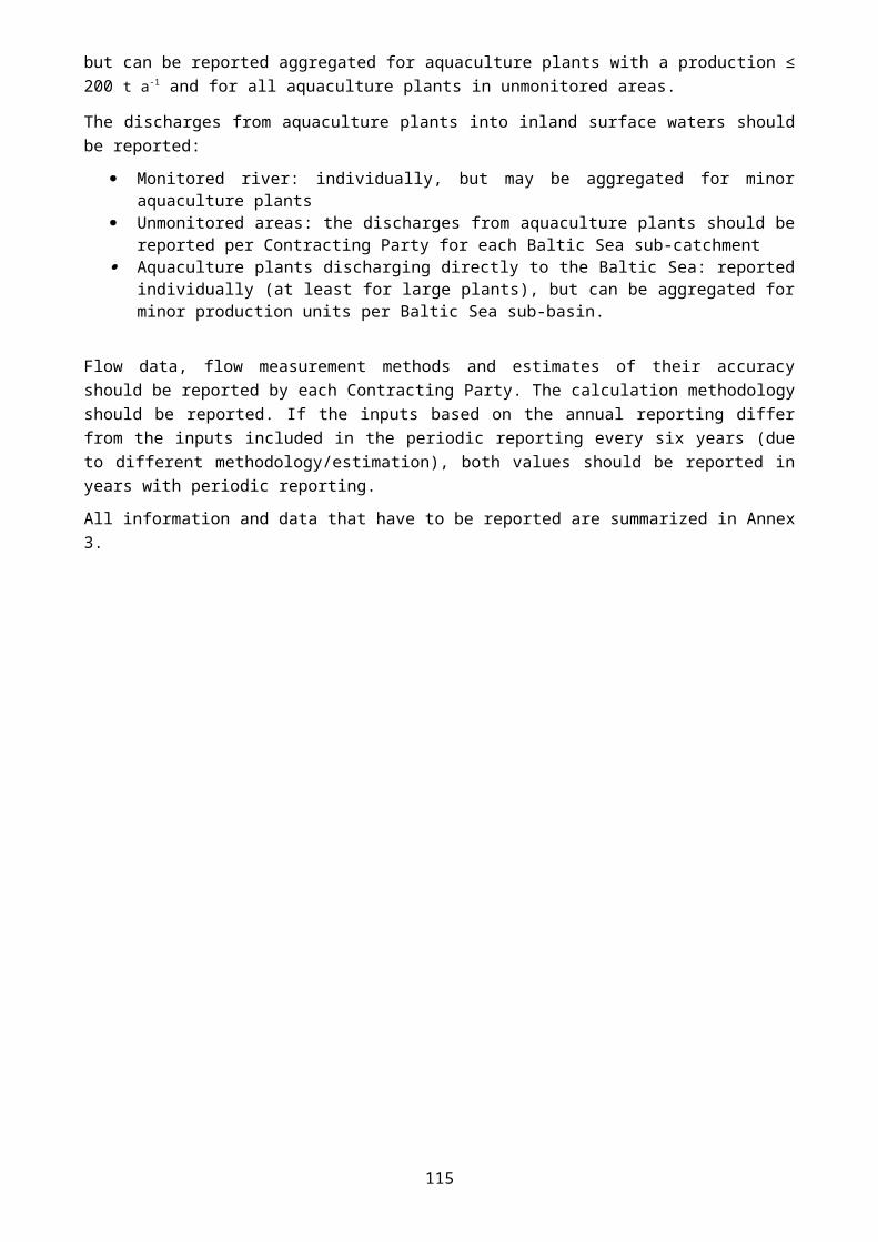
1) Minimum Reporting
a) Examples of discharges of industrial effluents to sub-catchments (direct or indirect)
Releases to water [kg/a] year 2012
Catchment national ID PRTR SECTOR CODE Release to water in kg ID year
SUN CHEMICAL A/S Zealand 5842 4 79 CuCHEMINOVA A/S Jutland and Funen 954 4 116 As, 22 NiPCK Raffinerie GmbH Schwedt River Oder 12-20730670000 1+4+5 66 Cr, 127 Cu, 106 Ni, 84.000 Ntot IDE0008 2006 and 2012VEO GmbH Eisenhüttenstadt River Oder 12-30670510000 1+5 61 Pb, 922 Zn, 132 Cyanides IDE0003 2012Eesti Energia Narva Elektrijaamad AS, Balti elektrijaam East Estonia EE051174 1+5 24 As, 13 Cd, 166 Cr, 167 Cu, 270 Pb
Kotkamills Oy Kymijoki-Gulf of Finland
1406 6 374 As, 25 Cd, 125 Cu, 5 Hg, 120 Ni,
Sachtleben Pigments OyKokemenjoki-Archipelago Sea-Bothnian Sea
2161 4 314 Cr, 1.210 Ni, 507 Zn
Akcinė bendrovė "LIFOSA" River Nemunas .000000005 4 447 Zn yesAkcinė bendrovė "Achema" River Nemunas .000000002 4 70 Cu, 190 Zn , 75.000 NtotGrupa LOTOS S.A. Vistula 11G000136 1 11 As, 86 Ni, 252 ZnZakłady Chemiczne "POLICE" S.A. - ODRA River Oder 16Z000445 1+4+5 53 As, 49 Hg, 2.320 Ni, 2.210 ZnSCA Östrands massafabrik - Bothnian sea Bothnian sea 2262-101 6 12 As, 39 Cd, 115 Cr, 547 Cu, 118 Ni, 37 Pb, 3540 ZnSt1 Refinery AB - Skagerrak and Kattegat Skagerrak and
Kattegat1480 - 1182 1 35 As, 29 Pb
EE
FI
LT
PL
SE
Country Point source / facility / plantPLC
DK
DE
PRTR
PLC details:
PLC examples from Germany
IDE0008 2 30,357076 tn/a IDE0003 2 20,25135008 tn/aIDE0008 4 Cd 0,001004 tn/a IDE0003 4 0,001058684 tn/aIDE0008 7 Cr 0,062267 tn/a IDE0003 7 0,004475348 tn/aIDE0008 8 Cu 0,094037 tn/a IDE0003 8 0,079509608 tn/aIDE0008 9 7.005.479 m3/a IDE0003 9 2406101 m3/aIDE0008 10 tn/a IDE0003 10 tn/a
IDE0008 11 Ni 0,086950 tn/a IDE0003 11 0,020223279 tn/a
IDE0008 12 68,455206 tn/a IDE0003 12 42,47971316 tn/a
IDE0008 13 0,420329 tn/a IDE0003 13 3,143971973 tn/aIDE0008 15 14,361232 tn/a IDE0003 15 2,634680595 tn/aIDE0008 16 97,726432 tn/a IDE0003 16 62,84735812 tn/aIDE0008 18 Pb 0,005709 tn/a IDE0003 18 0,089883913 tn/aIDE0008 20 0,443680 tn/a IDE0003 20 0,376955823 tn/aIDE0008 23 tn/a IDE0003 23 0,845664298 tn/a
PLC example from LithuaniaAchema Lifosa
3 17,520000 4,980000 tn/a
4 Cd tn/a
7 Cr 0,010000 tn/a8 Cu 0,070000 tn/a9 4.112.000 1.687.000 m3/a
10 tn/a11 Ni 0,010000 tn/a12 7,150000 0,780000 tn/a13 1,280000 0,220000 tn/a15 65,290000 10,280000 tn/a16 75,350000 14,080000 tn/a18 Pb 0,020000 tn/a20 2,570000 2,930000 tn/a23 0,190000 0,450000 tn/a
115

2) Enhanced Reporting
Permitting authorities regularly receive monitoring data from, or can request the operator of any plant or installation, to supply data. They are regularly asked to submit data (concentration values, load and flow data) to the national PLC data manager.
Enhanced Reporting = Minimum reporting + industrial point sources discharging to inland surface water or directly to the Baltic Sea but not registered in PRTRs. A possible criterion for identification of these sources could be based on the PRTR thresholds for releases to water (=100%) as follows: 100% > release ≥ 50% (Parameter and PRTR thresholds to water in Table xx).
Example of direct discharge: Sugar factory in Anklam/Germany, Plant code: IDE0015, subcatchment: BAPDESEA=SCDE00075
Example Indirect Discharges: VEO GmbH, Eisenhuettenstadt, Plant code: IDE0003, subcatchment: ODER=SCDE00035
116
PARAMETER ID
PARAMETER STATUS VALUE VALUE
UNIT
2 TOT 1,1994 tn/a
4 TOT 0,000008 tn/a
7 TOT 0,00268 tn/a
8 TOT 0,005689 tn/a
9 TOT 792881 m³/a
10 TOT 0,000004 tn/a
11 TOT 0,006738 tn/a
12 TOT 0,4549 tn/a
13 TOT 0,2004 tn/a
15 TOT 8,7979 tn/a
16 TOT 12,2101 tn/a
18 TOT 0,000102 tn/a
20 TOT 0,1799 tn/a
23 TOT 0,005797 tn/a
PARAMETER ID VALUE VALUE UNIT
2 20,251350 tn/a
4 0,001059 tn/a
7 0,004475 tn/a
8 0,079510 tn/a
9 2.406.101 m3/a
10 n.a. tn/a
11 0,020223 tn/a
12 42,479713 tn/a
13 3,143972 tn/a
15 2,634681 tn/a
16 62,847358 tn/a
18 0,089884 tn/a
20 0,376956 tn/a
23 0,845664 tn/a

The tables above contain data from the national permitting authority, which were included in the 2012 periodical report. The amount of releases indicates a rather small production volume/output of the plant where the PRTR threshold (see Table below) was not exceeded. Therefore, this plant was not registered in the national PRTR.
Table xx: Parameter and PRTR thresholds to water
PLC PRTRPRTR threshold for
releases to water [kg/a]Parameter ID Substance 100 % 50%
16 Total nitrogen 50.000 25.00020 Total phosphorus 5.000 2.500
Arsenic and compounds (as As) 5 2,54 Cadmium and compounds (as Cd) 5 2,57 Chromium and compounds (as Cr) 50 258 Copper and compounds (as Cu) 50 25
10 Mercury and compounds (as Hg) 1 0,511 Nickel and compounds (as Ni) 20 1018 Lead and compounds (as Pb) 20 1023 Zinc and compounds (as Zn) 100 50
3) Concluding remark
The focus on thresholds gives a hint to production capacity and size of the plant, which are not needed at all for PLC. While E-PRTR data for minimum reporting can be extracted from the register, data for enhanced reporting require very close cooperation with national authorities responsible for permitting and/or monitoring. Non-EU countries applying other rules are invited to strive for good correlation to these criteria and to measurements and analytical methods complying with international standards.
Checking the PRTR for industrial point sources is useful. Care must be taken as differences and potential inconsistencies exist between data reported under different reporting obligations. While only direct point sources are to be included in annual reporting, all industrial point sources (individually or aggregated) have to be included in periodical compilations.
End of Annex 6
117

Annex 7.EMEP assessment of atmospheric nitrogen and heavy metal deposition on the Baltic SeaEMEP has provided Annex 7.
EMEP prepares annual assessments for HELCOM of emissions and depositions of nitrogen, heavy metals and PCDD/Fs to the Baltic Sea. These are based on modelling and monitoring data which are annually presented to the Steering Body of EMEP in Geneva.
Assessing atmospheric nitrogen deposition on the Baltic Sea
The atmospheric depositions of oxidized and reduced nitrogen were calculated with the latest version of EMEP/MSC-W model in Oslo. The latest available official emission data for the HELCOM countries have been used in the model computations. Emissions of the two nitrogen species for each year of the period 1995-2010 were officially reported to the UN ECE Secretariat by several HELCOM Contracting Parties. Missing information was estimated by experts. Both official data and expert estimates were used for modelling atmospheric transport and deposition of nitrogen compounds to the Baltic Sea - http://www.ceip.at/.
Atmospheric depositions of oxidized and reduced nitrogen were computed for the entire EMEP domain, which includes Baltic Sea basin and catchment. Time series of annual atmospheric depositions are available for the period 1995 – 2010.
Atmospheric input and source allocation budgets of nitrogen (oxidized, reduced and total) to the Baltic Sea basins and catchments are computed using the latest version of EMEP/MSC-W model. EMEP/MSC-W model is a multipollutant, three-dimensional Eulerian model which takes into account processes of emission, advection, turbulent diffusion, chemical transformations, wet and dry depositions and inflow of pollutants into the model domain. Complete description of the model and its applications is available on the web http://www.emep.int. The results of the EMEP Unified model are routinely compared with available measurements at EMEP and HELCOM stations and the comparison of calculated versus measured data indicates that the model predicts the observed air concentrations of lead and cadmium within the accuracy of approximately 30%.
Calculations of atmospheric transport and depositions of nitrogen compounds are performed annually two years in arrears on the basis of emission data officially submitted by Parties to the Convention on Long-Range Transboundary Air Pollution Convention and expert estimates.
Assessing atmospheric heavy metal depositions to the Baltic Sea
Atmospheric deposition of lead, cadmium, and mercury were obtained for the European region and surrounding areas covered by the EMEP modelling domain and time-series of annual atmospheric deposition are available for the period 1990 – 2010.
Atmospheric input and source allocation budgets of heavy metals (cadmium, lead, and mercury) to the Baltic Sea and its catchment area have been computed using the latest version of MSCE-HM model, which is a regional-scale model operating within the EMEP region. This is a three-dimensional Eulerian model that includes processes of emission, advection, turbulent diffusion, chemical transformations of mercury, wet and dry deposition, and inflow of pollutant into the model domain. Horizontal grid of the model is defined using stereographic projection with spatial resolution 50 km at 60° latitude. The description of EMEP horizontal grid system can be found in the internet (http://www.emep.int/grid/index.html). The vertical structure of the model consists of 15 non-uniform layers defined in the terrain-following s-coordinates and
118

covers almost the whole troposphere. Detailed description of the model can be found in EMEP reports (Travnikov and Ilyin, 2005) and on the EMEP web page (http://www.emep.int). Meteorological data used in the calculations for 1990-2009 were obtained using MM5 meteorological data preprocessor on the basis of the Re-analysis project data prepared by National Centers for Environmental Predictions together with National Center of the Atmospheric Research (NCEP/NCAR) in the USA (http://wesley.ncep.noaa.gov/reanalysis.html)) and meteorological analysis of European Centre for Medium-Range Weather Forecasts (ECMWF).
The MSCE-HM model has been verified in a number of inter-comparison campaigns with other regional HM transport models (Sofiev et al., 1996; Gusev et al., 2000; Ryaboshapko et al., 2001, 2005) and has been qualified by means of sensitivity and uncertainty studies (Travnikov, 2000). It was concluded in these publications that the results of heavy metal airborne transport modelling were in satisfactory agreement with the available measurements and the discrepancies did not exceed on average a factor of two. The comparison of calculated versus measured data indicates that the model predicts the observed air concentrations of lead and cadmium within the accuracy of 30%. For concentrations in precipitation the difference between calculated and measured values may reach two times. Computed mercury concentrations deviate from measured values within a factor of two.
Calculations of atmospheric transport and deposition of lead, cadmium, and mercury are provided on the regular basis annually two years in arrears on the basis of emission data officially submitted by Parties to CLRTAP Convention.
Normalizing atmospheric deposition
In order to reduce the influence of meteorology on computed annual deposition an thus allow for better evaluation of the effectiveness of measures taken to reduce pollution loads, EMEP has developed a simple procedure for normalizing atmospheric deposition values. The following is a description of how EMEP have used the source-receptor matrices and depositions for calculating “normalized” depositions to the Baltic Sea for oxidized, reduced and total nitrogen and for each year of the period 1995-2010. The below equations were used for each of 16-year period 1995-2010 with available EMEP model runs.
The total nitrogen deposition to the Baltic Sea basin in the year iy can be calculated as:
Dtot ( iy )=Dox( iy )+Drd (iy )=∑i=1
ns1
A iox ( iy)×Ei
ox ( iy)+∑i=1
ns2
A ird( iy )×E i
rd (iy ) (A9.1)
where Dox ( iy ) and D
rd ( iy )is the annual total deposition of oxidized and reduced nitrogen, respectively, to the Baltic Sea in the year iy. The numbers of emission sources contributing to oxidized nitrogen deposition (ns1) and reduced nitrogen (ns2) are different in general, because some sources (e.g. ship traffic on the Baltic Sea) emit only oxidized nitrogen.
The annual depositions were calculated for each combination of meteorological and emission year:
Dox ( ie ,im )=∑i=1
ns1
Aox( im )×Eox( ie)+Rox( ie , im)
Drd ( ie , im )=∑i=1
ns 2
Ard ( im )×Erd ( ie)+Rrd ( ie ,im ) (A9.2)
Terms Rox ( ie ,im )and R
rd ( ie ,im )are introduce mainly because of the contribution of BIC (Initial and Boundary Conditions) in the model calculations, additional source for which emissions cannot be specified.
119
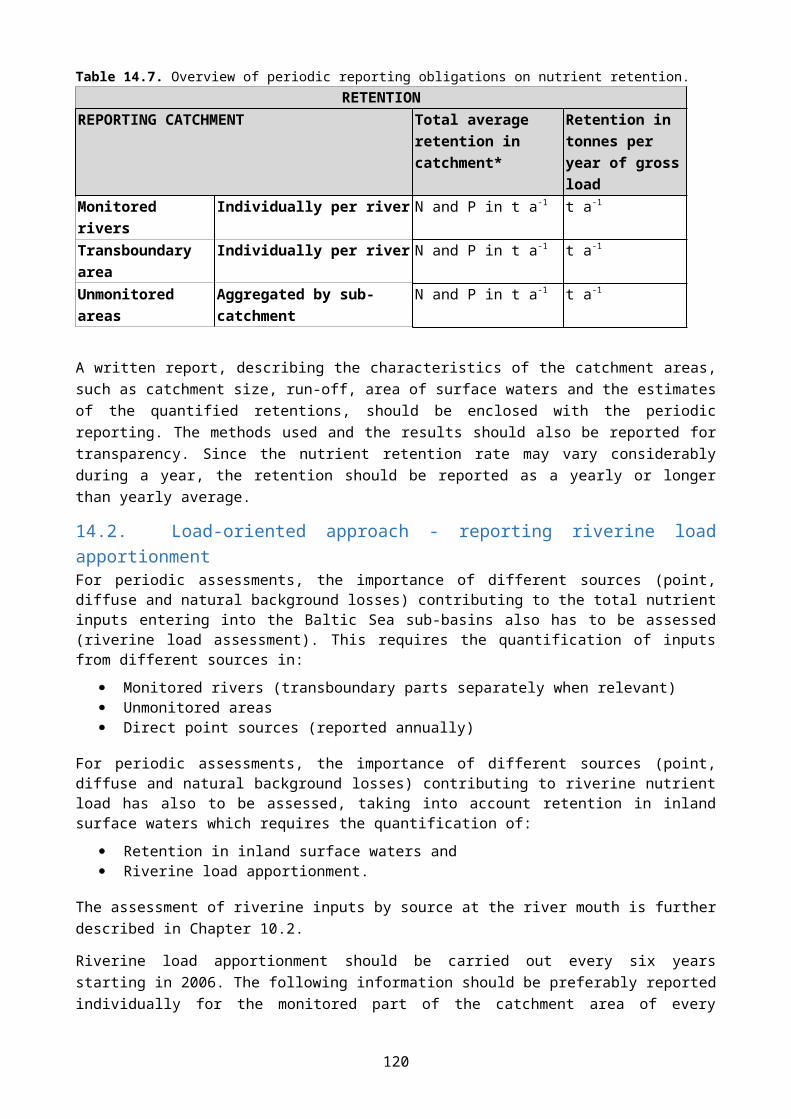
For the Baltic Sea basin this additional source is only contributing to oxidized nitrogen deposition, so.
Rrd ( ie ,im )=0 . The normalized deposition of total nitrogen for the emission year ie - DN(ie) is defined as:
DN ( ie)=MED {Dox ( ie ,1 )+Drd (ie ,1) ,. . ., Dox ( ie ,im )+Drd (ie , im) , .. . ,Dox( ie ,16)+Drd ( ie ,16 )} (A9.3)
Where MED is the median take over 16 values which correspond to 16 meteorological years. In addition, the maximum and minimum values are also calculated for each emission year. The results of these calculations for the years 1995-2010 are shown in the below Figure A1 for oxidized, reduced and total nitrogen deposition.
Normalized deposition of total nitrogen
Figure A1. Normalized depositions of total nitrogen for the period 1995-2010. Minimum, maximum and actual annual values of the deposition are also shown.
For more information, see the latest annual report prepared by EMEP (Atmospheric supply of nitrogen, lead, cadmium, mercury and dioxins/furans to the Baltic Sea in 2011) as well as the latest Baltic Sea Environment Fact Sheets on emissions and depositions of nitrogen, heavy metals and PCDDF/s, which can be accessed via the HELCOM website.
References
Gusev A., Ilyin I., Petersen G., van Pul A. & Syrakov D. 2000. Long-range transport model intercomparison studies. Model intercomparison study for cadmium. EMEP/ESC-E Report 2/2000, Meteorological Synthesizing Centre – East, Moscow, Russia. (http://www.msceast.org/reps/2_2000.zip)
Ryaboshapko A., Ilyin I., Bullock R., Ebinghaus R., Lohman K., Munthe J., Petersen G., Segneur C., & Wangberg I. 2001. Intercomparison study of numerical models for long-range atmospheric transport of mercury. Stage I: Comparison of chemical modules for mercury transformations in a cloud/fog environment. EMEP/MSC-E Technical report 2/2001, Meteorological Synthesizing Centre – East, Moscow, Russia. (http://www.msceast.org/abstract/201.html)
Ryaboshapko A., Artz R., Bullock R., Christensen J., Cohen M., Draxler R., Ilyin I., Munthe J., Pacyna J., Petersen G., Syrakov D., & Travnikov O. 2005. Intercomparison study of numerical models for long-range atmospheric transport of mercury. Stage III. Comparison of modelling results with long-term observations and comparison of calculated items of regional balances. EMEP/MSC-E Technical Report 1/2005, Meteorological Synthesizing Centre – East, Moscow, Russia. (http://www.msceast.org/reps/1_2005.zip)
120

Sofiev M., Maslyaev A. & Gusev A. 1996. Heavy metal model intercomparison. Methodology and results for Pb in 1990. EMEP/MSC-E Report 2/1996, Meteorological Synthesizing Centre - East, Moscow, Russia. (http://www.msceast.org/reps/2_1996.zip)
Travnikov O. 2000. Uncertainty analysis of heavy metals long-range transport modelling. EMEP/MSC-E Technical note 9/2000, Meteorological Synthesizing Centre - East, Moscow, Russia. (http://www.msceast.org/abstract/900.html)
Travnikov O. & Ilyin I. 2005. Regional Model MSCE-HM of Heavy Metal Transboundary Air Pollution in Europe. EMEP/MSC-E Technical Report 6/2005. (http://www.msceast.org/events/review/hm_description.html)
121

Annex 8.List of HELCOM PLC Contacts
Representing Name, Institute and e-mail addressDenmark Lars M. Svendsen, DCE - Danish Centre for Environment and Energy
[email protected] Boutrup (QA issues), DCE - Danish Centre for Environment and [email protected] Jytte Erfurt (reporting), DCE - Danish Centre for Environment and [email protected] E. Larsen (statistical methods), University of Aarhus,[email protected]
Estonia Peeter Ennet, Estonian Environment [email protected] Ulm, Ministry of [email protected]
Finland Seppo Knuuttila, Finnish Environment [email protected] Räike (reporting), Finnish Environment [email protected] Ruoho-Airola (atmospheric inputs), Finnish Meteorological [email protected]
Germany Dietmar Koch, Federal Environment [email protected]
Latvia Anete Šturma, Latvian Environment, Geology And Meteorology [email protected]
Lithuania Svajunas Plunge, Environmental Protection [email protected]
Poland Waldemar Jarosinski, Institute of Meteorology and Water Management, National Research [email protected] Robak-Bakierowska, Voivodship Inspectorate for Environmental [email protected]
Russia Natalia Oblomkova, Saint-Petersburg Public Organization "Ecology and Business"[email protected]
Sweden Lars Sonesten (QA issues), Swedish University of Agricultural Sciences, [email protected] Kaspersson (reporting), Swedish Agency for Marine and Water [email protected]
Data Manager Mr. Pekka Kotilainen, Finnish Environment [email protected]
122