NISTIR 7638

Guidelines for Accepting 2D Building Plans Geraldine S. Cheok James Filliben Alan M. Lytle

NISTIR 7638

Guidelines for Accepting 2D Building Plans Geraldine S. Cheok Building and Fire Research Laboratory James Filliben Information Technology Laboratory Alan M. Lytle Building and Fire Research Laboratory December 2008

U. S. Department of Commerce Carlos Gutierrez, Secretary

National Institute of Standards and Technology

Patrick D. Gallagher, Deputy Director

1

1. Introduction The General Services Administration’s (GSA) Public Buildings Services manages 1600 buildings totaling 180, 000, 000 square feet. GSA’s ability to capture, validate, and report the spatial information of its building assets (e.g., dimensions, areas, and locations of rooms; elevation details; HVAC and ductwork, etc) affects how GSA conducts its core business. To this end, GSA has been conducting pilot projects using 3D imaging systems to determine the efficacy of 3D imaging to capture and model existing conditions. The raw output of a 3D imaging system is in the form of point clouds (clouds of points numbering, typically, in the millions) which may be imported to CAD applications. The raw data are often post-processed to produce 2D documents (e.g., drawings, plans), 3D geometric models, and building information models (BIM). As 3D imaging is a relatively new technology, there are currently no standards for the evaluation of these instruments or the data (raw or derived). As a result, there are no standard methods to determine the accuracy of the deliverables other than physical inspection. This guideline is prepared to assist GSA project managers to objectively determine if a 2D building plan derived from 3D imaging data is within specification (in-spec) -- that is, this guideline provides a systematic answer to the question:

Are the dimensional deviations for the 2D plans within the specifications stated in the contract?

The methodology described in this guideline would also apply when evaluating 3D models. For the evaluation of point clouds (raw, not post-processed data), this methodology would also apply but the analysis potentially becomes much more complicated due to comparing the ensuing inspector data with raw service provider data (e.g., point cloud) versus summarized (e.g., 2D building plans or 3D models) service provider data.

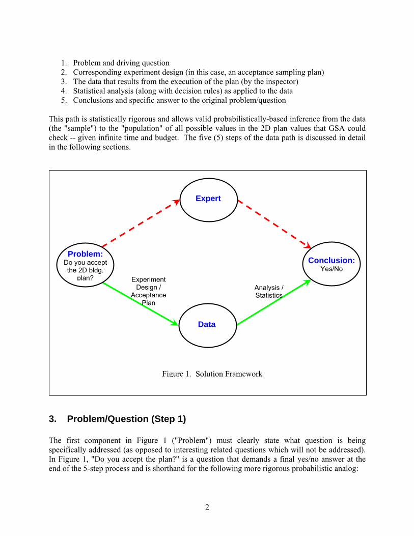
2. Solution Framework/Structure Although the GSA responsibility will involve the acceptance or rejection of a 2D plan with respect to a specific building, the general acceptance/rejection problem (and its solution) has a generic statistical structure. Figure 1 illustrates the framework in which we may move from the original question to a rigorously valid answer to that question. The top path (the "expert path") in Figure 1 indicates a course to a solution based solely on expert judgment as opposed one based on data. Although both paths will lead to a solution (not necessarily the same), the expert path is included only for completeness and is not recommended per se, since it does not lend itself to the calculation of rigorous and scientifically-defensible confidence levels. The bottom path (the "data path") in Figure 1 is the recommended path with five (5) components:

2

1. Problem and driving question 2. Corresponding experiment design (in this case, an acceptance sampling plan) 3. The data that results from the execution of the plan (by the inspector) 4. Statistical analysis (along with decision rules) as applied to the data 5. Conclusions and specific answer to the original problem/question

This path is statistically rigorous and allows valid probabilistically-based inference from the data (the "sample") to the "population" of all possible values in the 2D plan values that GSA could check -- given infinite time and budget. The five (5) steps of the data path is discussed in detail in the following sections.

3. Problem/Question (Step 1) The first component in Figure 1 ("Problem") must clearly state what question is being specifically addressed (as opposed to interesting related questions which will not be addressed). In Figure 1, "Do you accept the plan?" is a question that demands a final yes/no answer at the end of the 5-step process and is shorthand for the following more rigorous probabilistic analog:

Experiment Design /

Acceptance Plan

Analysis / Statistics

Figure 1. Solution Framework

Problem: Do you accept the 2D bldg.

plan?

Expert

Data

Conclusion: Yes/No

3

Is GSA 95 % (say) confident that 99 % (say) of the all of the dimensions of the entire building are "in-spec"?

The 95 % value given in the above statement is typical in scientific investigations. The 99 % value is given as an example -- GSA must specify the preferred values (see Section 4.2).

4. Experiment Design / Acceptance Sampling Plan (Step 2) Component 2 in Figure 1 is entitled Experiment Design1 / Acceptance Sampling. Experiment Design is the general statistical designation of all activities encompassing the problem classification, problem translation, design construction, and design execution that links the original specification of the problem to an actual dataset. There are many kinds of scientific problems which in turn lead to many types of experiment plans. For the case at hand, we wish to accept/reject a larger (typically unattainable) set of items of interest (the population -- the entire 2D plan) from a smaller (attainable) subset of items (the "sample"). This case is structurally characterized as statistical "hypothesis testing" (as opposed to "estimation") with the additional constraint that the data is binary, go/no-go, in-spec/out-of-spec. Such a subset of experiment design is generically referred to as "Acceptance Sampling" and has the benefit of a large and robust literature. At first blush, it is seen that there are at least five different strategies (experiment designs) that GSA could exercise in assessing the quality of 2D plans for a building:

1. No checking 2. "Random" spot checks 3. 100 % sampling 4. Randomized acceptance sampling 5. Stratified randomized acceptance sampling

Each of these five strategies has a cost (both money and time) and a risk associated with it - the risk of rejecting a deliverable that should be accepted and accepting a deliverable that should be rejected. These strategies are discussed in detail below.

4.1 Experiment Designs

4.1.1 No Checking Strategy 1 (no checking) has zero cost but has enormous risk. Since this strategy basically accepts the inspector's word and reputation at face value, there are no data and hence, no data-based probabilistic link is possible to allow a rigorous answer to the above 95 % / 99 % question. This strategy is thus not to be recommended.

1 Experiment design is used synonymously with experimental design.

4

4.1.2 "Random" Spot Checks Strategy 2 (spot checking) is a commonly-employed procedure (used by GSA in the past) whereby an inspector may perform "random" sampling for a limited (e.g., 1 day) length of time. This strategy incurs some limited cost, but still has considerable risk because it is not random "enough". The seemingly random/unpredictable nature of the sampling is in fact human-based, i.e., arbitrary, and hence is not sufficiently rigorous to the point of allowing the formation of valid confidence statements about the population (the entire 2-D plan) as a whole. Although commonly used, this strategy is not recommended since it provides no methodology to allow us to make the statement: "I (GSA) am 95 % (say) confident that 99 % (say) of the all of the dimensions of the entire building are "in-spec".

4.1.3 100 % Sampling This "brute force" strategy dictates that the inspector check every dimension in the 2-D plan. Properly done (e.g., calibrated measurement device, known environmental conditions), this strategy will yield a rigorous and unambiguous answer to the question as to what proportion of the population of building dimensions are "in-spec". The downside of this strategy is, of course, the cost -- both in time and money. This strategy also tends to give a false sense of security (as suggested by its name) as discussed in [1], especially pages 431-434.

4.1.4 Randomized Acceptance Sampling (RAS) This strategy entails assigning an index to each member of the population, and then randomly drawing a (small) subset of that population in such a fashion that each and every member of the population has an equal chance of being drawn. The virtue of this strategy is twofold: it is both cost-efficient (with relatively small expenditure of time and money), and statistically rigorous (which allows valid statistical inferences to be made about the population). A disadvantage of this strategy is that it may lead to an under representation of certain characteristics features of the population’s members.

In the absence, however, of any other information about the population [the building(s) in GSA’s case], this is a special case of Acceptance Sampling based solely on randomized data collection, and would be a recommended strategy of choice.

4.1.5 Stratified Randomized Acceptance Sampling (SRAS) This strategy is an extension and an improvement over the Randomized Acceptance Sampling. It is an extension in that it includes in the sampling process additional information which helps assure that the resulting sample serves as a more representative surrogate of the population. That is, information about building characteristics (number of floors, room type, etc. - see Section 4.3.2) will be incorporated in the acceptance sampling strategy to assure that the proportions in the resulting sample (number of measurements per floor, per room type, etc.) is equivalent to that of the target population. For simple Randomized Acceptance Sampling, such balanced proportionality will occur "on the average"; for Stratified Randomized Acceptance Sampling, such balance is "forced" and is not "left to chance". For example, for a building with three

5

levels, the SRAS method will ensure that measurements are taken from all three levels whereas the potential exists in the RAS method where measurements are only taken from only the second and third levels or where the majority of the measurements are on one level. The net result is that the SRAS strategy results are less prone to bias and variability, and more robust to known building characteristics than RAS, and hence SRAS is our recommended strategy of choice. Because of these advantages, the SRAS method is used by most professional polling/survey organizations.

Another distinction between SRAS and RAS is the issue of randomization. For RAS, the formal, statistical randomization is done at the global level -- giving all elements of the population an equal chance of being drawn. For SRAS, the randomization is done at the local level -- after stratification is carried out on as many factors as identified, the remaining elements of that stratified subset of the population are given an equal chance of being drawn.

4.2 Required GSA Inputs for the Experiment Design The SRAS method has an extensive literature that outlines not only the methodology but also the user inputs that are required to provide a valid answer to the question:

Is GSA 95 % (say) confident that 99 % (say) of the all of the dimensions of the entire building are "in spec"?

For a specific 2D-plan under evaluation, the development and construction of the corresponding Acceptance Sampling plan would necessitate GSA-provided information for the following items:

1. Tolerance, T 2. Maximum % of population out-of-spec, P 3. Sample size, n

In the above question, the value of 95 % is described in section 4.2.4 and the value of 99 % is described in Section 4.2.2

4.2.1 Tolerance, T The tolerance, T, is the maximum error that a measurement could have before GSA would declare the measurement to be "out-of-spec". It is noted that:

1. The value T may be different for different types of measurements and could be set equal to the different tolerances specified in the contract.

2. T can be specified absolutely or relatively, e.g., T: ± 6mm (1/4 in) or T: ± 5 %.

6

Why important? The Acceptance Plan that will be constructed will have a corresponding test statistic = the observed number of defectives out of the n measurements. The value T defined here will determine if a measurement is defective or not. The quantity to be checked (A) must lie within (M - T) and (M + T), i.e., (M - T) ≤ A ≤ (M + T) for it to be in-spec. For example, if the door width was one of the measurements to be checked in a 2D plan, then A = door width as obtained from the 2D plan and M = the measurement of the door width as reported by an inspector. The following would then be true: (M - T) ≤ A ≤ (M + T) in-spec (not defective)

Either A < (M - T) or A > (M + T) out-of-spec (defective)

4.2.2 Maximum % population out-of-spec, P P is the maximum percent of the population that is out-of-spec that is tolerable to GSA. This value answers the question:

For GSA to accept a 2D Plan, what is the largest percent defective (out-of-spec) of the whole population that would be tolerable to GSA?

Why important?

a. Whereas the tolerance value T in item 1 is a local specification which defines whether an individual measurement is "good enough" (in-spec or out-of-spec), the requested P value is a global specification which defines as to whether the totality of measurements from the 2D plan would be "good enough" (acceptable or unacceptable). If GSA does not define the maximum percent out-of-spec that it desires for the population, then it is impossible to arrive at a accept/reject decision rule for the analysis of the data resulting from the constructed acceptance plan.

b. The required statistical sample size n (see Section 4.2.3) critically depends on this value of P.

4.2.3 Sample size, n n is the number of measurements that will be made by the inspector; statistically, n is referred to as the "sample size". This number will depend largely on time and cost that GSA is willing to expend to perform the quality check. Acceptance plans may be constructed/developed for any sample size, n, and any population acceptance percentage P. However, the specification of maximum affordable sample size eliminates the consideration of theoretically optimal sample size values that are not practical

7

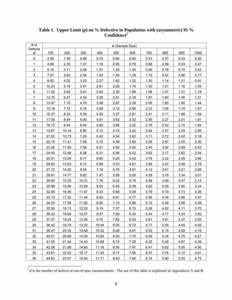
(i.e., beyond budget). Note that if P is severe enough (e.g., GSA will not accept the 2D plan unless GSA is 95 % confident that less than 0.0001 of the population is out-of-spec, then this would dictate a statistically large sample size to achieve such confidence. There is a trade off between P and n, and it may be possible that the (P, n) specification may yield no viable acceptance plan. Table 1 can be used to ascertain what is possible and is provided at the end of Section 4. This table is a critical component of the Acceptance Sampling plan. Note that Table 1 is based only on pass/fail binomial considerations. It makes no distribution, for example normality, assumptions about the underlying response and hence is “robust”. Table 1 is, thus, appropriate for a wide variety of applications. The use and interpretation of Table 1 is detailed in Appendices A and B.

4.2.4 Confidence Confidence = the degree of certainty that the final conclusion of accepting/rejecting the 2D plan is correct. All of our calculations will utilize a confidence value of 95 %, which is the most common value utilized in rigorous scientific studies. Note that Table 1 was generated based on a confidence level of 95 % (the values in Table 1 will change for a different confidence level).

4.2.5 Population, N The population size, N, is the maximum number of measurements to be made in the specific building under evaluation.

Population size is NOT a required input. However, since the ultimate inference is about the population as opposed to the sample (subset) that the inspector collects, the following discussion on “population” is presented for clarification.

In a typical GSA 2D-plan acceptance/rejection problem, the population is defined as the set of all building measurements that could be taken that will be compared to the corresponding dimensions in the 2D plan. In reality, this set could be infinitely large, but it is nevertheless important to conceptualize as to what this set is and is not. Inferences from the Acceptance Sampling strategy will yield conclusions about the population -- not just the collected sample from the population. The ultimate acceptance/rejection of the 2D plan will be contingent on the percent of the population -- not just the sample -- that are deemed to be "in spec". The point of this discussion is that the concept of "population" is critical to the appropriate interpretation and use of acceptance sample.

One useful metric of the population is its size. In the statistical literature, this is typically denoted by N. For small populations, the assignment of a value to N is very important; for large populations -- typical of building evaluations that GSA would see -- the assignment of a specific value is not as critical. In either case, it is of use to think of N as a fixed (even if unknown) value that designates the simplest characteristic of the population -- its size.

8

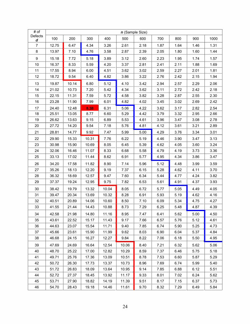
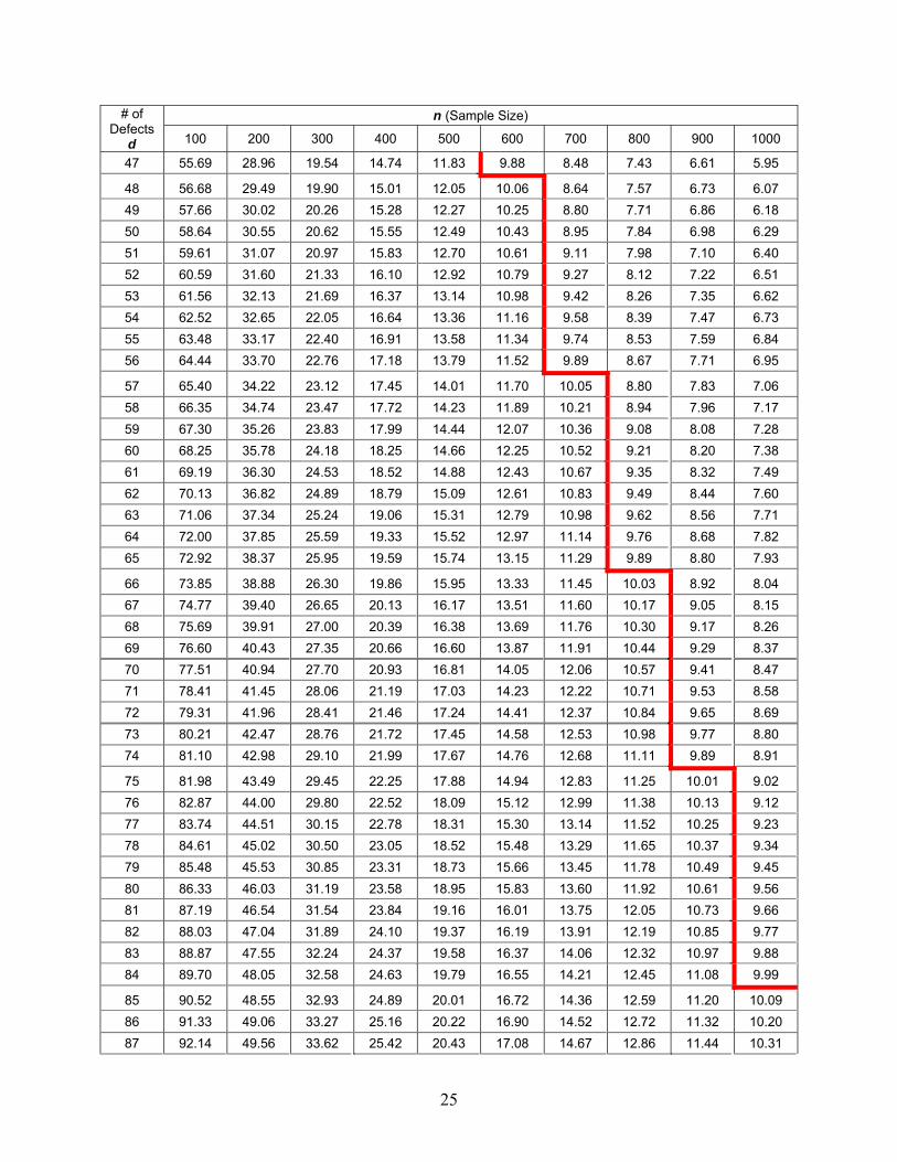
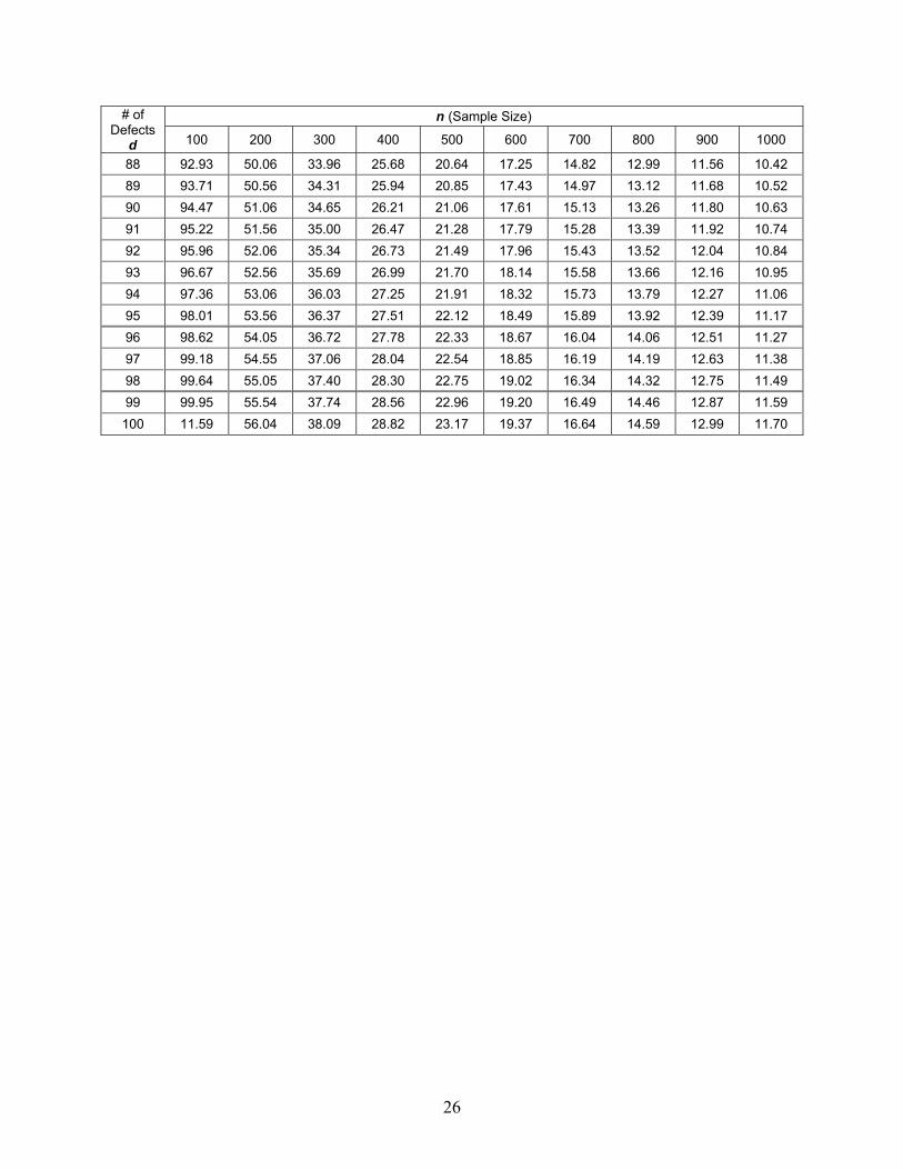
Table 1. Upper Limit (p) on % Defective in Population with (asymmetric) 95 % Confidence2

# of

Defects d

n (Sample Size)

100 200 300 400 500 600 700 800 900 1000 0 2.95 1.49 0.99 0.75 0.60 0.50 0.43 0.37 0.33 0.30 1 4.66 2.35 1.57 1.18 0.95 0.79 0.68 0.59 0.53 0.47 2 6.16 3.11 2.08 1.57 1.25 1.05 0.90 0.78 0.70 0.63 3 7.57 3.83 2.56 1.93 1.54 1.29 1.10 0.97 0.86 0.77 4 8.92 4.52 3.03 2.27 1.82 1.52 1.30 1.14 1.01 0.91 5 10.23 5.18 3.47 2.61 2.09 1.74 1.50 1.31 1.16 1.05 6 11.50 5.83 3.91 2.94 2.35 1.96 1.68 1.47 1.31 1.18 7 12.75 6.47 4.34 3.26 2.61 2.18 1.87 1.64 1.46 1.31 8 13.97 7.10 4.76 3.58 2.87 2.39 2.05 1.80 1.60 1.44 9 15.18 7.72 5.18 3.89 3.12 2.60 2.23 1.95 1.74 1.57

10 16.37 8.33 5.59 4.20 3.37 2.81 2.41 2.11 1.88 1.69 11 17.55 8.94 6.00 4.51 3.62 3.02 2.59 2.27 2.01 1.81 12 18.72 9.54 6.40 4.82 3.86 3.22 2.76 2.42 2.15 1.94 13 19.87 10.14 6.80 5.12 4.10 3.42 2.94 2.57 2.29 2.06 14 21.02 10.73 7.20 5.42 4.34 3.62 3.11 2.72 2.42 2.18 15 22.15 11.31 7.59 5.72 4.58 3.82 3.28 2.87 2.55 2.30 16 23.28 11.90 7.99 6.01 4.82 4.02 3.45 3.02 2.69 2.42 17 24.40 12.48 8.38 6.31 5.06 4.22 3.62 3.17 2.82 2.54 18 25.51 13.05 8.77 6.60 5.29 4.42 3.79 3.32 2.95 2.66 19 26.62 13.63 9.15 6.89 5.53 4.61 3.96 3.47 3.08 2.78 20 27.72 14.20 9.54 7.18 5.76 4.81 4.12 3.61 3.21 2.89 21 28.81 14.77 9.92 7.47 5.99 5.00 4.29 3.76 3.34 3.01 22 29.90 15.33 10.31 7.76 6.22 5.19 4.46 3.90 3.47 3.13 23 30.98 15.90 10.69 8.05 6.45 5.39 4.62 4.05 3.60 3.24 24 32.06 16.46 11.07 8.33 6.68 5.58 4.79 4.19 3.73 3.36 25 33.13 17.02 11.44 8.62 6.91 5.77 4.95 4.34 3.86 3.47 26 34.20 17.58 11.82 8.90 7.14 5.96 5.12 4.48 3.99 3.59 27 35.26 18.13 12.20 9.19 7.37 6.15 5.28 4.62 4.11 3.70 28 36.32 18.69 12.57 9.47 7.60 6.34 5.44 4.77 4.24 3.82 29 37.37 19.24 12.95 9.75 7.82 6.53 5.61 4.91 4.37 3.93 30 38.42 19.79 13.32 10.04 8.05 6.72 5.77 5.05 4.49 4.05 31 39.47 20.34 13.69 10.32 8.28 6.91 5.93 5.19 4.62 4.16 32 40.51 20.89 14.06 10.60 8.50 7.10 6.09 5.34 4.75 4.27 33 41.55 21.44 14.43 10.88 8.73 7.29 6.25 5.48 4.87 4.39 34 42.58 21.98 14.80 11.16 8.95 7.47 6.41 5.62 5.00 4.50 35 43.61 22.52 15.17 11.43 9.17 7.66 6.57 5.76 5.12 4.61 36 44.63 23.07 15.54 11.71 9.40 7.85 6.74 5.90 5.25 4.73

2 d is the number of defects or out-of-spec measurements. The use of this table is explained in Appendices A and B.

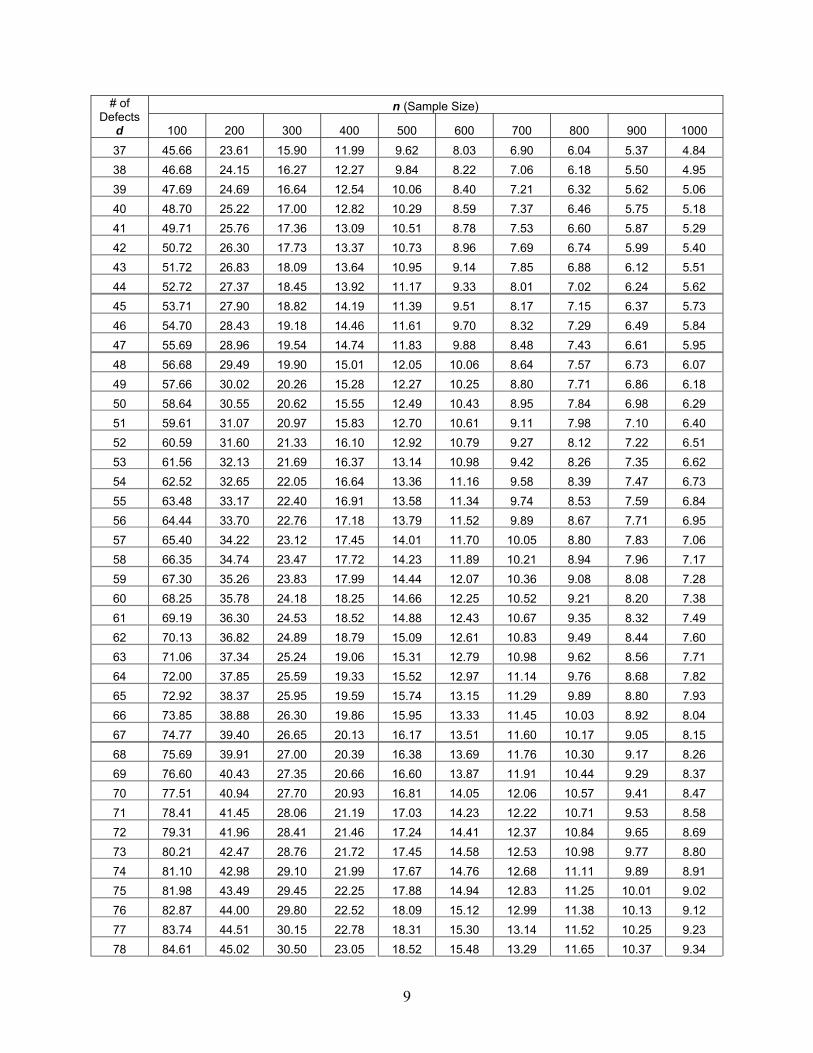
9

# of Defects

d

n (Sample Size)

100 200 300 400 500 600 700 800 900 1000 37 45.66 23.61 15.90 11.99 9.62 8.03 6.90 6.04 5.37 4.84 38 46.68 24.15 16.27 12.27 9.84 8.22 7.06 6.18 5.50 4.95 39 47.69 24.69 16.64 12.54 10.06 8.40 7.21 6.32 5.62 5.06 40 48.70 25.22 17.00 12.82 10.29 8.59 7.37 6.46 5.75 5.18 41 49.71 25.76 17.36 13.09 10.51 8.78 7.53 6.60 5.87 5.29 42 50.72 26.30 17.73 13.37 10.73 8.96 7.69 6.74 5.99 5.40 43 51.72 26.83 18.09 13.64 10.95 9.14 7.85 6.88 6.12 5.51 44 52.72 27.37 18.45 13.92 11.17 9.33 8.01 7.02 6.24 5.62 45 53.71 27.90 18.82 14.19 11.39 9.51 8.17 7.15 6.37 5.73 46 54.70 28.43 19.18 14.46 11.61 9.70 8.32 7.29 6.49 5.84 47 55.69 28.96 19.54 14.74 11.83 9.88 8.48 7.43 6.61 5.95 48 56.68 29.49 19.90 15.01 12.05 10.06 8.64 7.57 6.73 6.07 49 57.66 30.02 20.26 15.28 12.27 10.25 8.80 7.71 6.86 6.18 50 58.64 30.55 20.62 15.55 12.49 10.43 8.95 7.84 6.98 6.29 51 59.61 31.07 20.97 15.83 12.70 10.61 9.11 7.98 7.10 6.40 52 60.59 31.60 21.33 16.10 12.92 10.79 9.27 8.12 7.22 6.51 53 61.56 32.13 21.69 16.37 13.14 10.98 9.42 8.26 7.35 6.62 54 62.52 32.65 22.05 16.64 13.36 11.16 9.58 8.39 7.47 6.73 55 63.48 33.17 22.40 16.91 13.58 11.34 9.74 8.53 7.59 6.84 56 64.44 33.70 22.76 17.18 13.79 11.52 9.89 8.67 7.71 6.95 57 65.40 34.22 23.12 17.45 14.01 11.70 10.05 8.80 7.83 7.06 58 66.35 34.74 23.47 17.72 14.23 11.89 10.21 8.94 7.96 7.17 59 67.30 35.26 23.83 17.99 14.44 12.07 10.36 9.08 8.08 7.28 60 68.25 35.78 24.18 18.25 14.66 12.25 10.52 9.21 8.20 7.38 61 69.19 36.30 24.53 18.52 14.88 12.43 10.67 9.35 8.32 7.49 62 70.13 36.82 24.89 18.79 15.09 12.61 10.83 9.49 8.44 7.60 63 71.06 37.34 25.24 19.06 15.31 12.79 10.98 9.62 8.56 7.71 64 72.00 37.85 25.59 19.33 15.52 12.97 11.14 9.76 8.68 7.82 65 72.92 38.37 25.95 19.59 15.74 13.15 11.29 9.89 8.80 7.93 66 73.85 38.88 26.30 19.86 15.95 13.33 11.45 10.03 8.92 8.04 67 74.77 39.40 26.65 20.13 16.17 13.51 11.60 10.17 9.05 8.15 68 75.69 39.91 27.00 20.39 16.38 13.69 11.76 10.30 9.17 8.26 69 76.60 40.43 27.35 20.66 16.60 13.87 11.91 10.44 9.29 8.37 70 77.51 40.94 27.70 20.93 16.81 14.05 12.06 10.57 9.41 8.47 71 78.41 41.45 28.06 21.19 17.03 14.23 12.22 10.71 9.53 8.58 72 79.31 41.96 28.41 21.46 17.24 14.41 12.37 10.84 9.65 8.69 73 80.21 42.47 28.76 21.72 17.45 14.58 12.53 10.98 9.77 8.80 74 81.10 42.98 29.10 21.99 17.67 14.76 12.68 11.11 9.89 8.91 75 81.98 43.49 29.45 22.25 17.88 14.94 12.83 11.25 10.01 9.02 76 82.87 44.00 29.80 22.52 18.09 15.12 12.99 11.38 10.13 9.12 77 83.74 44.51 30.15 22.78 18.31 15.30 13.14 11.52 10.25 9.23 78 84.61 45.02 30.50 23.05 18.52 15.48 13.29 11.65 10.37 9.34

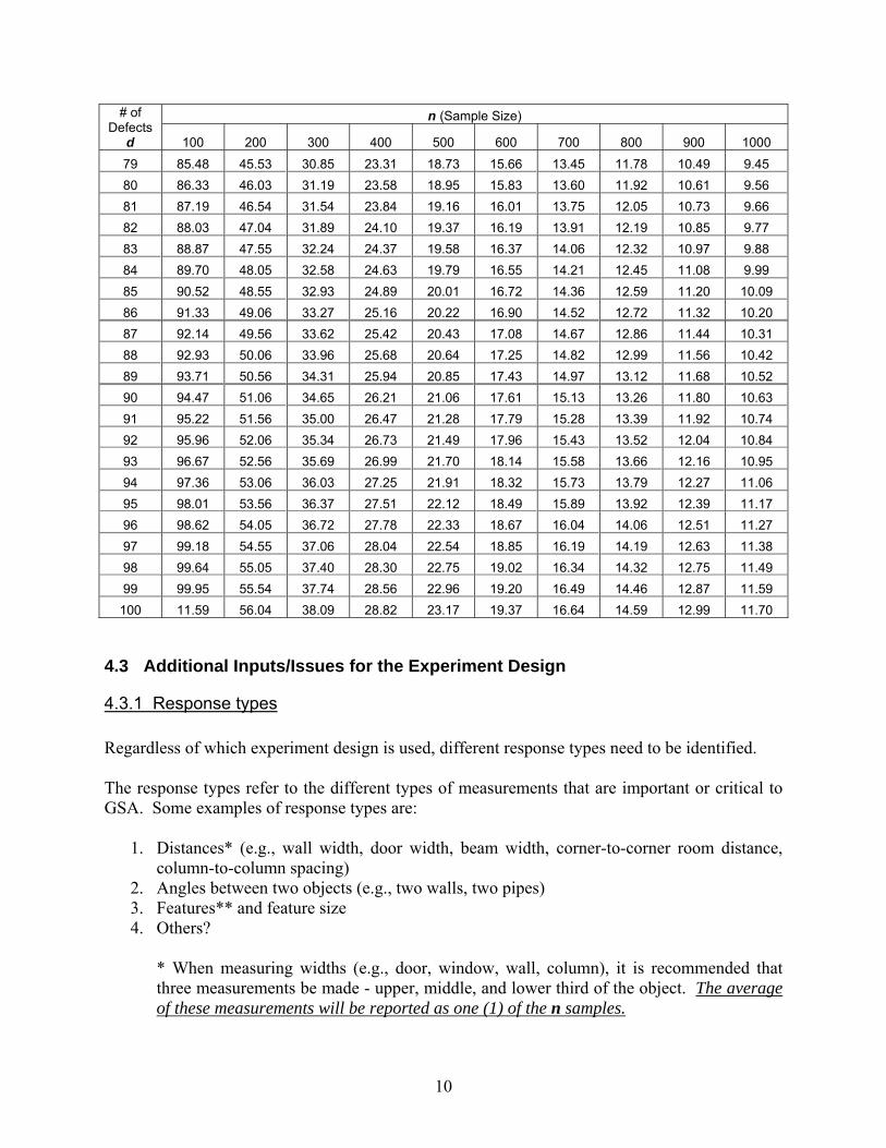
10

# of Defects

d

n (Sample Size)

100 200 300 400 500 600 700 800 900 1000 79 85.48 45.53 30.85 23.31 18.73 15.66 13.45 11.78 10.49 9.45 80 86.33 46.03 31.19 23.58 18.95 15.83 13.60 11.92 10.61 9.56 81 87.19 46.54 31.54 23.84 19.16 16.01 13.75 12.05 10.73 9.66 82 88.03 47.04 31.89 24.10 19.37 16.19 13.91 12.19 10.85 9.77 83 88.87 47.55 32.24 24.37 19.58 16.37 14.06 12.32 10.97 9.88 84 89.70 48.05 32.58 24.63 19.79 16.55 14.21 12.45 11.08 9.99 85 90.52 48.55 32.93 24.89 20.01 16.72 14.36 12.59 11.20 10.09 86 91.33 49.06 33.27 25.16 20.22 16.90 14.52 12.72 11.32 10.20 87 92.14 49.56 33.62 25.42 20.43 17.08 14.67 12.86 11.44 10.31 88 92.93 50.06 33.96 25.68 20.64 17.25 14.82 12.99 11.56 10.42 89 93.71 50.56 34.31 25.94 20.85 17.43 14.97 13.12 11.68 10.52 90 94.47 51.06 34.65 26.21 21.06 17.61 15.13 13.26 11.80 10.63 91 95.22 51.56 35.00 26.47 21.28 17.79 15.28 13.39 11.92 10.74 92 95.96 52.06 35.34 26.73 21.49 17.96 15.43 13.52 12.04 10.84 93 96.67 52.56 35.69 26.99 21.70 18.14 15.58 13.66 12.16 10.95 94 97.36 53.06 36.03 27.25 21.91 18.32 15.73 13.79 12.27 11.06 95 98.01 53.56 36.37 27.51 22.12 18.49 15.89 13.92 12.39 11.17 96 98.62 54.05 36.72 27.78 22.33 18.67 16.04 14.06 12.51 11.27 97 99.18 54.55 37.06 28.04 22.54 18.85 16.19 14.19 12.63 11.38 98 99.64 55.05 37.40 28.30 22.75 19.02 16.34 14.32 12.75 11.49 99 99.95 55.54 37.74 28.56 22.96 19.20 16.49 14.46 12.87 11.59 100 11.59 56.04 38.09 28.82 23.17 19.37 16.64 14.59 12.99 11.70

4.3 Additional Inputs/Issues for the Experiment Design

4.3.1 Response types Regardless of which experiment design is used, different response types need to be identified. The response types refer to the different types of measurements that are important or critical to GSA. Some examples of response types are:

1. Distances* (e.g., wall width, door width, beam width, corner-to-corner room distance, column-to-column spacing)

2. Angles between two objects (e.g., two walls, two pipes) 3. Features** and feature size 4. Others?

* When measuring widths (e.g., door, window, wall, column), it is recommended that three measurements be made - upper, middle, and lower third of the object. The average of these measurements will be reported as one (1) of the n samples.

11

** This would not be part of a 2D plan but there were previous GSA projects where features needed to be identified (e.g., cracks greater than 12 mm, spalling of roof tiles) - this would be a check of whether the feature was identified or not.

An indication (by GSA) should also be made as to the relative importance of the above items/responses. For this unequal weights case, an additional (analysis) complication arises in that a method would have to be developed to determine Pass/Fail. For example, if there are 5 failures/defects for responses with a high weight and 10 failures/defects for responses with a lower weight, how does one “combine” these values to “calculate” the final Pass/Fail of the deliverable?

4.3.2 Factors In addition, if the choice of an experiment design is our recommended SRAS (Stratified Randomized Acceptance Sampling), then GSA would need to provide additional information to assist in that stratification, namely, relevant building factors and characteristics:

1. Number of floors 2. Room type - this can be grouped based on:

a. Room function (e.g., office, restroom, conference room, closet, stairwell) b. Room size (e.g., square footage).

3. “Type” of distance - a. Examples include door width, wall width, length of hallway, width of hallway,

window width b. It is recommended that various distances be included - short distances (e.g., door

width), mid-range distances (e.g., wall width), and long distances (e.g., length of hallway).

4. Areas of interest as called out in the contract 5. Others?

GSA's provision of these factors is important because it will allow for the construction of an acceptance plan that is not just random, but also balanced, and hence more representative of the entire building (the "population"). If random but unbalanced, then it could be possible that some important measurements may be missing (e.g., conference room), or most of the measurements could (by chance) be made on only one floor level or one part of the building.

4.4 Other Questions/Issues for the Experiment Design The following items do not required immediate information from GSA. They do, however, encompass "ground truth" issues with the inspector measurements which generically affect -- to a degree beyond responses, factors, and experiment design -- the validity of GSA's final acceptance/rejection decision:

1. Measuring device (method & accuracy) 2. Operator

12

3. Replication

4.4.1 Device Two critical questions regarding device are:

a. How accurate is it? b. How accurate must it be to assess the quality (or lack of quality) of the 2-D drawing?

Our recommendation is to follow the common practice in the scientific arena, whereby ground truth (i.e., inspector) measurements should be an order of magnitude better than the 2-D drawings being evaluated. Some devices are:

a. Tape measure b. Total station or EDM (Electronic Distance Measuring) instrument c. 3D imaging system

Each of these devices has different intrinsic accuracy. Measurements obtained using a tape would probably be the quickest but they would probably have the most noise associated with them (see Section 4.4.2 for some reasons). There have not been any comprehensive studies to compare the accuracy of measurements from a total station with those from a 3D imaging system, and there are different opinions as to which is more accurate. To minimize the instrument uncertainties, calibrated instruments should be used and compensations/corrections for environmental factors should also be made.

4.4.2 Operator Operator error contributes to the uncertainties of the “truth” measurements. It is almost a given that two operators will obtain different measurements of a given object. The difference will likely be greater if a tape measure was used - different tape tension, different points measured, different tape reading (rounding). The training and skill level of the operator significantly affects the quality of inspector measurements.

4.4.3. Replication Replication is important in general because it allows an independent assessment of the total error of the measurement process, based on collected data -- as opposed to an assessment based on a priori engineering "best guesses" and manufacturer specifications. Further, when inspector devices are known to have intrinsic uncertainties which are not an order of magnitude better (as recommended in Section 4.4.1), then replication allows the use of averages which intrinsically have smaller uncertainties than any single value.

13

5. Data (Step 3) Step 3 in the solution process (see Figure 1) is the execution of the prescribed experiment design /acceptance sampling plan, with the ensuing collection of n inspector measurement values (the data). It is recommended that this resulting dataset be “vectorized” (column) in format--with one line per measurement. If it is determined that the maximum affordable number of observations is n = 200, then the resulting dataset should have n = 200 lines (rows) and (r + k) columns where r is the number of responses measured (see Section 4.3.1) and k is the number of factors (see Section 4.3.2) specified. Note that the quality of the dataset is bounded by the quality of the experiment design/ acceptance sample that was constructed and executed for the sampling. In particular, a poor experiment design or "sloppy" execution of the experiment design will result in a dataset that is deficient in content and will severely limit, if not exclude, inferences to the population. This information deficiency cannot be repaired -- no matter how sophisticated the statistical analysis--and so it is of paramount importance to construct and execute the best experiment design/ acceptance sampling plan possible.

6. Analysis (Step 4) Step 4 in the process (see Figure 1) is the statistical analysis of the data. If an appropriate experiment design/ acceptance sampling plan were executed, then the data analysis protocol is as follows:

1. For each line of the data file, a. Compare the tabulated inspector data with the data derived from the 2D plan.

Let M = inspector measurement, A = corresponding measurement derived from 2D plan, and T is the GSA-specified tolerance (see Section 4.2.1). Compare A to (M ± T).

b. Determine if the measurement is: i. 0 = "in spec", or

ii. 1 = "out of spec" = defect c. Record conclusion in a new column

2. Sum up the total number of defects d. This sum will be a value between a. 0 (= all measurements are "in spec"), and b. n (= all measurements are "out of spec")

3. Go to Table 1 and find the appropriate (row, column) entry p as dictated by (row = d =

number of defects , column = n = number of samples). For this (d, n) combination, the cell entry p is our data-based estimate of the maximum percent defective in the population. Based on the data on hand, we will be 95 %

14

confident that the true (unknown, and unknowable) number of measurements defective in the population will be p or less.

4. Compare p with P where P is the GSA-specified (in Section 4.2.2) maximum acceptable

value for the percent defective for the population -- above which would result in rejecting the 2D plan. By comparing p with P, we thus arrive at a rigorous decision rule by which GSA may rigorously accept or reject the 2D plan.

5. The global decision rule for the whole population is:

a. If p ≤ P, then accept the 2D plan. b. If p > P, then reject the 2D plan.

7. Conclusions (Step 5) By conducting the above 5-step analysis protocol, GSA may rigorously arrive at a decision (accept or reject) for the 2D building plan. If the decision is to reject, GSA will have to determine a course of action such as:

- Course 1: Reject 2D plan - Course 2:

1. Contractor corrects errors and re-submits plans 2. GSA re-conducts acceptance sampling 3. Accept/reject 2D plan

- Course 3: 1. Conduct additional sampling 2. If the decision is to again “reject”, then “reject” 2D plan 3. If the decision it to accept, then GSA will need to make an executive decision

whether to accept or reject the 2D plan. Regardless of the course of action selected, the method of accept/reject of the deliverable should be made clear to the service providers and should be a part of the statement-of-work. Although additional computational complications may exist, a similar 5-step protocol may be used to form acceptance/rejection conclusions for 3D plans and for point clouds.

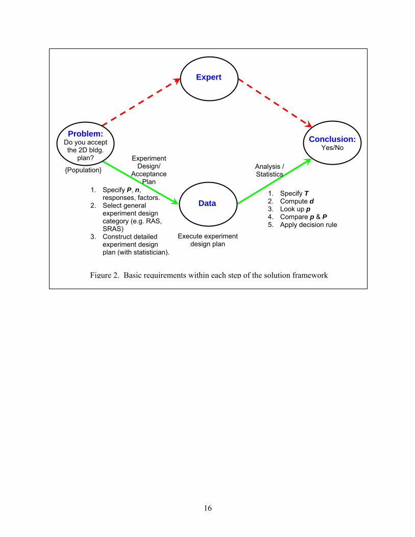
8. Procedures for Developing an Acceptance Sampling Plan Figure 2 shows the 5-step process for the framework to accept/ reject a deliverable and when inputs are required. A more detail description of the 5-step process follows:

1. Determine and list each measurement type (name and description) that is important. (Section 4.3.1).

2. Specify how the measurements are to be made. The step includes: a. Specifying the type of instrument used to obtain the measurements b. Proof of calibration of the instrument and any required in-field checks

15

c. Describing how the measurements are to be obtained. For example, i. Are measurements to be made multiple times and reporting the average?

ii. If a door width is to be measured, where should be the measurements be made?

3. Specify the criteria for conformity for each type of measurement. Clearly describe when the measurement is “in-spec” or “out-of-spec” (defective).

4. Develop the sampling plan a. Define tolerance, T (Section 4.2.1) b. Define P (Section 4.2.2) c. Define sample size, n (Section 4.2.3)

5. Select Experiment Design a. Randomized Acceptance Sampling (Section 4.1.4) b. Stratified Randomized Acceptance Sampling (Section 4.1.5)

6. Develop in conjunction with a statistician an Experiment Design based on the Response Types and Factors (Section. 4.3).

a. If there are no existing plans, then the determination of which measurements to make will have to be performed “manually”. For example, manually identify the doors, randomly select the required number of doors.

b. If there are existing plans, there is on-going research to automate this process, i.e., automatically extract the doors from the plans, generate the list, and randomly select the doors.

7. Execute Experiment Design (Section 5) 8. Analyze the data to obtain d (Section 6) 9. Use Table 1, accept or reject (Section 6). If reject,

a. Reject deliverable, OR b. Conduct additional sampling, OR c. Contractor corrects errors and re-submits plans and GSA conducts acceptance

sampling plan again

9. References 1. Stephens, Kenneth S., (2001), "The Handbook of Applied Acceptance Sampling", ASQ

Press, Milwaukee, WI.

16

Experiment Design/

Acceptance Plan

Analysis / Statistics {Population}

Figure 2. Basic requirements within each step of the solution framework

Problem: Do you accept the 2D bldg.

plan?

Data

Expert

Conclusion: Yes/No

1. Specify P, n, responses, factors.

2. Select general experiment design category (e.g. RAS, SRAS)

3. Construct detailed experiment design plan (with statistician).

1. Specify T 2. Compute d 3. Look up p 4. Compare p & P 5. Apply decision rule

Execute experiment design plan

17

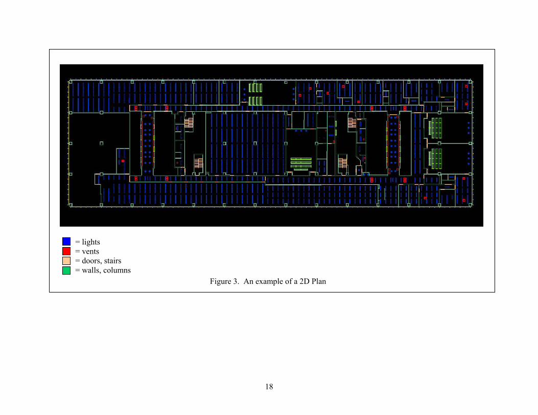
Appendix A - An Example Given a 2D Building Plan (see Figure 3), the Problem/Question is: Does GSA accept this 2D plan? For this example, the following are measurements of interest or considered critical:

1. Response Y1 = wall length 2. Response Y2 = door widths 3. Response Y3 = column widths

For simplicity, we will only examine a single response, Y = Y1 (wall length). Thus, the specifications given below will refer to wall length only. These input specifications (set by GSA) could differ for the other responses. The conclusions will be specific to a response, and hence a building plan may, for example, be acceptable with respect to Y1 (wall length) and Y2 (door width), but unacceptable with respect to Y3 (column width). As discussed in Section 4.3.1, if the responses have different weights, then a method will have to be developed to determine Accept/Reject of the 2D plan. On the other hand, all three responses could be combined into one response, Y = distances (e.g., wall length, door width, column width, hallway width). If the decision is to reject, then some of the options available are stated in Section 7.

18

Figure 3. An example of a 2D Plan

= lights = vents = doors, stairs = walls, columns

19

For Response Y = Y1 = wall length, the specifications are:

1. Tolerance, T = 13 mm (1/2 in) 2. Maximum Percent Defective P for the Population = 10 % 3. Maximum practical/affordable sample size, n = 200

where n is based on a. time (1 day) b. cost ($5000) - measuring device (e.g., tape, total station)

We thus have P = 10%, n = 200. The experiment design for such a problem is given in Section 4.1:

• Section 4.1.4 - RAS (Randomized Acceptance Sampling) or • Section 4.1.5 - SRAS (Stratified Randomized Acceptance Sampling) - Preferred

The construction and execution of either of the above experiment design can have subtleties and a statistician should be consulted in developing the experiment design (e.g., how many measurements per level, rooms in which the wall lengths are obtained, etc.). Let’s say a statistician was consulted, the experiment design plan has been executed, and 200 inspector measurements of wall length were collected. The following 2 cases are examined:

Case 1 If there were exactly d = 15 defects (out of 200), then this yields a percent defective in our sample P̂ = d/n =15/200 = 7.5 %. Given this 7.5 % defective for the sample and given that GSA's acceptance/rejection criterion is P = 10 % defective for the population, then

Can GSA rigorously state with 95 % confidence that the population defect is in fact 10 % or less (and hence accept the 2D plan for Y = Y1 = wall length)?

Solution: Referring to Table 1, for n = 200 (column 3) and d = 15, the corresponding cell entry, p, is 11.31 %. This means that GSA can with 95 % confidence state that the percent defective for the population is ≤ 11.31%, but cannot with 95 % confidence state that P is ≤ 10 %. Since 11.31 % exceeds the initially specified 10 % (p ≥ P, see Section 6, step 5b), then GSA must reject the 2D plan. Case 2 If the observed number of defects were d = 9 (out of the 200), then this yields a percent defective in our sample P̂ = d/n = 9/200 = 4.5 %. Given this 4.5 % defective for the sample and given that GSA's acceptance/rejection criterion is P = 10 % defective for the population, then

20

Can GSA rigorously state with 95 % confidence that the population defect is in fact 10 % or less (and hence accept the 2D plan for Y = Y1 = wall length)?

Solution: Referring to Table 1, for n = 200 (column 3) and d = 9, the corresponding cell entry, p, is 7.72 %. This means that GSA can with 95 % confidence state that the percent defective for the population is ≤ 7.72%. Since 7.72 % is less than the initially specified 10 % (p ≤ P, see Section 6, step 5a), then GSA can accept the 2D plan.

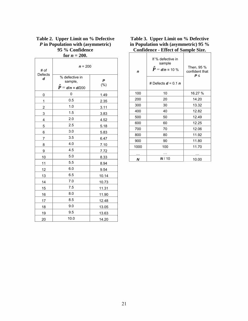
A.1 Discussion Exercises similar to Cases 1 and 2 may be repeated. A subset of Table 1 for n = 200 and d = 1 to 20 is presented in Table 2. In Table 2, the second column lists the percent defective in the sample while the third column lists the percent defective of the population. Interpreting Table 2:

For n = 200, if GSA observes d (column 1) defects in the sample, then GSA is 95 % confident that the percent defective P (column 3) in the population is less than p (value in cell entry).

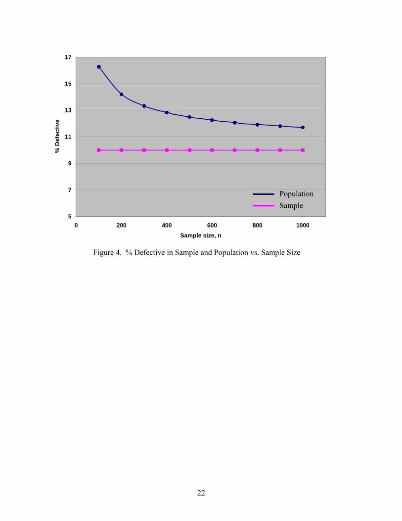
In Table 2, a comparison of the second and third columns ( P̂ vs. P ) shows that the percent defective, P̂ , in the sample is necessarily less than the estimate of the upper limit of the (true) percent defective, P, in the population. Note that the values in the 3rd column are upper limits for P; and note that the true (unknown) P for the population could be either less than OR greater than our observed P̂ . As the sample size gets larger (i.e., the sample approaches the population), the differences between P̂ and P will get smaller. This is shown in Table 3 where as n approaches N, the % defect in both the sample and the population are equal. It is also of note that there is a point at which increasing sample size does not yield a corresponding increase in benefit (Figure 4) - it this case, n is about 400 or 500.

21

Table 2. Upper Limit on % Defective P in Population with (asymmetric)

95 % Confidence for n = 200.

# of Defects

d

n = 200

% defective in sample,

P̂ = d/n = d/200

P (%)

0 0 1.49

1 0.5 2.35

2 1.0 3.11

3 1.5 3.83

4 2.0 4.52

5 2.5 5.18

6 3.0 5.83

7 3.5 6.47

8 4.0 7.10

9 4.5 7.72

10 5.0 8.33

11 5.5 8.94

12 6.0 9.54

13 6.5 10.14

14 7.0 10.73

15 7.5 11.31

16 8.0 11.90

17 8.5 12.48

18 9.0 13.05

19 9.5 13.63

20 10.0 14.20

Table 3. Upper Limit on % Defective in Population with (asymmetric) 95 %

Confidence - Effect of Sample Size.

n

If % defective in

sample

P̂ = d/n = 10 %

Then, 95 % confident that

P ≤

# Defects d = 0.1 n

100 10 16.27 % 200 20 14.20 300 30 13.32 400 40 12.82 500 50 12.49 600 60 12.25 700 70 12.06 800 80 11.92 900 90 11.80

1000 100 11.70

… … … N N / 10 10.00

22

Figure 4. % Defective in Sample and Population vs. Sample Size

5

7

9

11

13

15

17

0 200 400 600 800 1000Sample size, n

% D

efec

tive

Population Sample

23

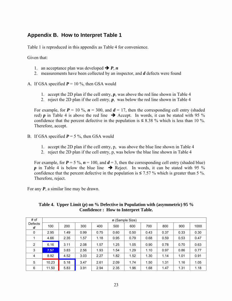
Appendix B. How to Interpret Table 1 Table 1 is reproduced in this appendix as Table 4 for convenience. Given that:

1. an acceptance plan was developed P, n 2. measurements have been collected by an inspector, and d defects were found

A. If GSA specified P = 10 %, then GSA would

1. accept the 2D plan if the cell entry, p, was above the red line shown in Table 4 2. reject the 2D plan if the cell entry, p, was below the red line shown in Table 4

For example, for P = 10 %, n = 300, and d = 17, then the corresponding cell entry (shaded red) p in Table 4 is above the red line Accept. In words, it can be stated with 95 % confidence that the percent defective in the population is ≤ 8.38 % which is less than 10 %. Therefore, accept.

B. If GSA specified P = 5 %, then GSA would

1. accept the 2D plan if the cell entry, p, was above the blue line shown in Table 4 2. reject the 2D plan if the cell entry, p, was below the blue line shown in Table 4

For example, for P = 5 %, n = 100, and d = 3, then the corresponding cell entry (shaded blue) p in Table 4 is below the blue line Reject. In words, it can be stated with 95 % confidence that the percent defective in the population is ≤ 7.57 % which is greater than 5 %. Therefore, reject.

For any P, a similar line may be drawn.

Table 4. Upper Limit (p) on % Defective in Population with (asymmetric) 95 % Confidence : How to Interpret Table.

# of

Defects d

n (Sample Size)

100 200 300 400 500 600 700 800 900 1000

0 2.95 1.49 0.99 0.75 0.60 0.50 0.43 0.37 0.33 0.30 1 4.66 2.35 1.57 1.18 0.95 0.79 0.68 0.59 0.53 0.47

2 6.16 3.11 2.08 1.57 1.25 1.05 0.90 0.78 0.70 0.63 3 7.57 3.83 2.56 1.93 1.54 1.29 1.10 0.97 0.86 0.77 4 8.92 4.52 3.03 2.27 1.82 1.52 1.30 1.14 1.01 0.91

5 10.23 5.18 3.47 2.61 2.09 1.74 1.50 1.31 1.16 1.05 6 11.50 5.83 3.91 2.94 2.35 1.96 1.68 1.47 1.31 1.18

24

# of Defects

d

n (Sample Size)

100 200 300 400 500 600 700 800 900 1000

7 12.75 6.47 4.34 3.26 2.61 2.18 1.87 1.64 1.46 1.31 8 13.97 7.10 4.76 3.58 2.87 2.39 2.05 1.80 1.60 1.44

9 15.18 7.72 5.18 3.89 3.12 2.60 2.23 1.95 1.74 1.57 10 16.37 8.33 5.59 4.20 3.37 2.81 2.41 2.11 1.88 1.69 11 17.55 8.94 6.00 4.51 3.62 3.02 2.59 2.27 2.01 1.81 12 18.72 9.54 6.40 4.82 3.86 3.22 2.76 2.42 2.15 1.94

13 19.87 10.14 6.80 5.12 4.10 3.42 2.94 2.57 2.29 2.06 14 21.02 10.73 7.20 5.42 4.34 3.62 3.11 2.72 2.42 2.18 15 22.15 11.31 7.59 5.72 4.58 3.82 3.28 2.87 2.55 2.30 16 23.28 11.90 7.99 6.01 4.82 4.02 3.45 3.02 2.69 2.42

17 24.40 12.48 8.38 6.31 5.06 4.22 3.62 3.17 2.82 2.54 18 25.51 13.05 8.77 6.60 5.29 4.42 3.79 3.32 2.95 2.66 19 26.62 13.63 9.15 6.89 5.53 4.61 3.96 3.47 3.08 2.78 20 27.72 14.20 9.54 7.18 5.76 4.81 4.12 3.61 3.21 2.89

21 28.81 14.77 9.92 7.47 5.99 5.00 4.29 3.76 3.34 3.01

22 29.90 15.33 10.31 7.76 6.22 5.19 4.46 3.90 3.47 3.13 23 30.98 15.90 10.69 8.05 6.45 5.39 4.62 4.05 3.60 3.24 24 32.06 16.46 11.07 8.33 6.68 5.58 4.79 4.19 3.73 3.36 25 33.13 17.02 11.44 8.62 6.91 5.77 4.95 4.34 3.86 3.47

26 34.20 17.58 11.82 8.90 7.14 5.96 5.12 4.48 3.99 3.59 27 35.26 18.13 12.20 9.19 7.37 6.15 5.28 4.62 4.11 3.70 28 36.32 18.69 12.57 9.47 7.60 6.34 5.44 4.77 4.24 3.82 29 37.37 19.24 12.95 9.75 7.82 6.53 5.61 4.91 4.37 3.93

30 38.42 19.79 13.32 10.04 8.05 6.72 5.77 5.05 4.49 4.05 31 39.47 20.34 13.69 10.32 8.28 6.91 5.93 5.19 4.62 4.16 32 40.51 20.89 14.06 10.60 8.50 7.10 6.09 5.34 4.75 4.27 33 41.55 21.44 14.43 10.88 8.73 7.29 6.25 5.48 4.87 4.39

34 42.58 21.98 14.80 11.16 8.95 7.47 6.41 5.62 5.00 4.50 35 43.61 22.52 15.17 11.43 9.17 7.66 6.57 5.76 5.12 4.61 36 44.63 23.07 15.54 11.71 9.40 7.85 6.74 5.90 5.25 4.73 37 45.66 23.61 15.90 11.99 9.62 8.03 6.90 6.04 5.37 4.84 38 46.68 24.15 16.27 12.27 9.84 8.22 7.06 6.18 5.50 4.95

39 47.69 24.69 16.64 12.54 10.06 8.40 7.21 6.32 5.62 5.06 40 48.70 25.22 17.00 12.82 10.29 8.59 7.37 6.46 5.75 5.18 41 49.71 25.76 17.36 13.09 10.51 8.78 7.53 6.60 5.87 5.29 42 50.72 26.30 17.73 13.37 10.73 8.96 7.69 6.74 5.99 5.40 43 51.72 26.83 18.09 13.64 10.95 9.14 7.85 6.88 6.12 5.51 44 52.72 27.37 18.45 13.92 11.17 9.33 8.01 7.02 6.24 5.62 45 53.71 27.90 18.82 14.19 11.39 9.51 8.17 7.15 6.37 5.73 46 54.70 28.43 19.18 14.46 11.61 9.70 8.32 7.29 6.49 5.84

25

# of Defects

d

n (Sample Size)

100 200 300 400 500 600 700 800 900 1000

47 55.69 28.96 19.54 14.74 11.83 9.88 8.48 7.43 6.61 5.95

48 56.68 29.49 19.90 15.01 12.05 10.06 8.64 7.57 6.73 6.07 49 57.66 30.02 20.26 15.28 12.27 10.25 8.80 7.71 6.86 6.18 50 58.64 30.55 20.62 15.55 12.49 10.43 8.95 7.84 6.98 6.29 51 59.61 31.07 20.97 15.83 12.70 10.61 9.11 7.98 7.10 6.40 52 60.59 31.60 21.33 16.10 12.92 10.79 9.27 8.12 7.22 6.51 53 61.56 32.13 21.69 16.37 13.14 10.98 9.42 8.26 7.35 6.62 54 62.52 32.65 22.05 16.64 13.36 11.16 9.58 8.39 7.47 6.73 55 63.48 33.17 22.40 16.91 13.58 11.34 9.74 8.53 7.59 6.84 56 64.44 33.70 22.76 17.18 13.79 11.52 9.89 8.67 7.71 6.95

57 65.40 34.22 23.12 17.45 14.01 11.70 10.05 8.80 7.83 7.06 58 66.35 34.74 23.47 17.72 14.23 11.89 10.21 8.94 7.96 7.17 59 67.30 35.26 23.83 17.99 14.44 12.07 10.36 9.08 8.08 7.28 60 68.25 35.78 24.18 18.25 14.66 12.25 10.52 9.21 8.20 7.38 61 69.19 36.30 24.53 18.52 14.88 12.43 10.67 9.35 8.32 7.49 62 70.13 36.82 24.89 18.79 15.09 12.61 10.83 9.49 8.44 7.60 63 71.06 37.34 25.24 19.06 15.31 12.79 10.98 9.62 8.56 7.71 64 72.00 37.85 25.59 19.33 15.52 12.97 11.14 9.76 8.68 7.82 65 72.92 38.37 25.95 19.59 15.74 13.15 11.29 9.89 8.80 7.93

66 73.85 38.88 26.30 19.86 15.95 13.33 11.45 10.03 8.92 8.04 67 74.77 39.40 26.65 20.13 16.17 13.51 11.60 10.17 9.05 8.15 68 75.69 39.91 27.00 20.39 16.38 13.69 11.76 10.30 9.17 8.26 69 76.60 40.43 27.35 20.66 16.60 13.87 11.91 10.44 9.29 8.37 70 77.51 40.94 27.70 20.93 16.81 14.05 12.06 10.57 9.41 8.47 71 78.41 41.45 28.06 21.19 17.03 14.23 12.22 10.71 9.53 8.58 72 79.31 41.96 28.41 21.46 17.24 14.41 12.37 10.84 9.65 8.69 73 80.21 42.47 28.76 21.72 17.45 14.58 12.53 10.98 9.77 8.80 74 81.10 42.98 29.10 21.99 17.67 14.76 12.68 11.11 9.89 8.91

75 81.98 43.49 29.45 22.25 17.88 14.94 12.83 11.25 10.01 9.02 76 82.87 44.00 29.80 22.52 18.09 15.12 12.99 11.38 10.13 9.12 77 83.74 44.51 30.15 22.78 18.31 15.30 13.14 11.52 10.25 9.23 78 84.61 45.02 30.50 23.05 18.52 15.48 13.29 11.65 10.37 9.34 79 85.48 45.53 30.85 23.31 18.73 15.66 13.45 11.78 10.49 9.45 80 86.33 46.03 31.19 23.58 18.95 15.83 13.60 11.92 10.61 9.56 81 87.19 46.54 31.54 23.84 19.16 16.01 13.75 12.05 10.73 9.66 82 88.03 47.04 31.89 24.10 19.37 16.19 13.91 12.19 10.85 9.77 83 88.87 47.55 32.24 24.37 19.58 16.37 14.06 12.32 10.97 9.88 84 89.70 48.05 32.58 24.63 19.79 16.55 14.21 12.45 11.08 9.99

85 90.52 48.55 32.93 24.89 20.01 16.72 14.36 12.59 11.20 10.09 86 91.33 49.06 33.27 25.16 20.22 16.90 14.52 12.72 11.32 10.20 87 92.14 49.56 33.62 25.42 20.43 17.08 14.67 12.86 11.44 10.31

26

# of Defects

d

n (Sample Size)

100 200 300 400 500 600 700 800 900 1000

88 92.93 50.06 33.96 25.68 20.64 17.25 14.82 12.99 11.56 10.42 89 93.71 50.56 34.31 25.94 20.85 17.43 14.97 13.12 11.68 10.52 90 94.47 51.06 34.65 26.21 21.06 17.61 15.13 13.26 11.80 10.63 91 95.22 51.56 35.00 26.47 21.28 17.79 15.28 13.39 11.92 10.74 92 95.96 52.06 35.34 26.73 21.49 17.96 15.43 13.52 12.04 10.84 93 96.67 52.56 35.69 26.99 21.70 18.14 15.58 13.66 12.16 10.95 94 97.36 53.06 36.03 27.25 21.91 18.32 15.73 13.79 12.27 11.06 95 98.01 53.56 36.37 27.51 22.12 18.49 15.89 13.92 12.39 11.17 96 98.62 54.05 36.72 27.78 22.33 18.67 16.04 14.06 12.51 11.27 97 99.18 54.55 37.06 28.04 22.54 18.85 16.19 14.19 12.63 11.38 98 99.64 55.05 37.40 28.30 22.75 19.02 16.34 14.32 12.75 11.49 99 99.95 55.54 37.74 28.56 22.96 19.20 16.49 14.46 12.87 11.59 100 11.59 56.04 38.09 28.82 23.17 19.37 16.64 14.59 12.99 11.70