High PerformanceSwitching and RoutingTelecom Center Workshop: Sept 4, 1997.

Guaranteed Smooth Scheduling in Packet Switches

Isaac Keslassy (Stanford University), Murali Kodialam, T.V. Lakshman, Dimitri Stiliadis (Bell-Labs)

Outline

1. Frame Scheduling

2. GLJD Algorithm

3. GLJD Guarantees

4. Simulations

5. Conclusion

Crossbar

Scheduler

inputs

outputs

1

N

1 N

.

.

.

.

. . . .

Packet Switch Scheduling

012

113

001

Frame-Based Scheduling

1 2

1

1

0 1 2

2 0 1 , 3

1 2 0

0 0 1 0 1 0

2 1 0 0 1 0 0 1

0 1 0 1 0 0

0 0 1 0 0 1 0 1 0 0 0 1

1 0 0 , 1 0 0 , 0 0 1 1 0

0 1 0 0 1 0 1 0 0

K

k kk

M M

cycle

R F

R M

Cycle

2

0 0 1 0 1 0

0 , 1 0 0 , 0 0 1

0 1 0 0 1 0 1 0 0

cycle

Example:

Frame-Based Scheduling• Traffic Demand Matrix:

– Given a frame size of F, and an NxN integer demand matrix R of row and column sum equal to F

– Can we send Rij amount of traffic from i to j during any frame?

• Birkhoff-von Neumann (BvN) Decomposition: We can decompose R as a sum of K < N2 weighted permutations, with

the weight sum equal to F.

• Frame-Scheduling: Apply BvN decomposition, then cycle through the permutations (C.S

Chang et al., 2000).FMR

K

kk

K

kkk

11

,

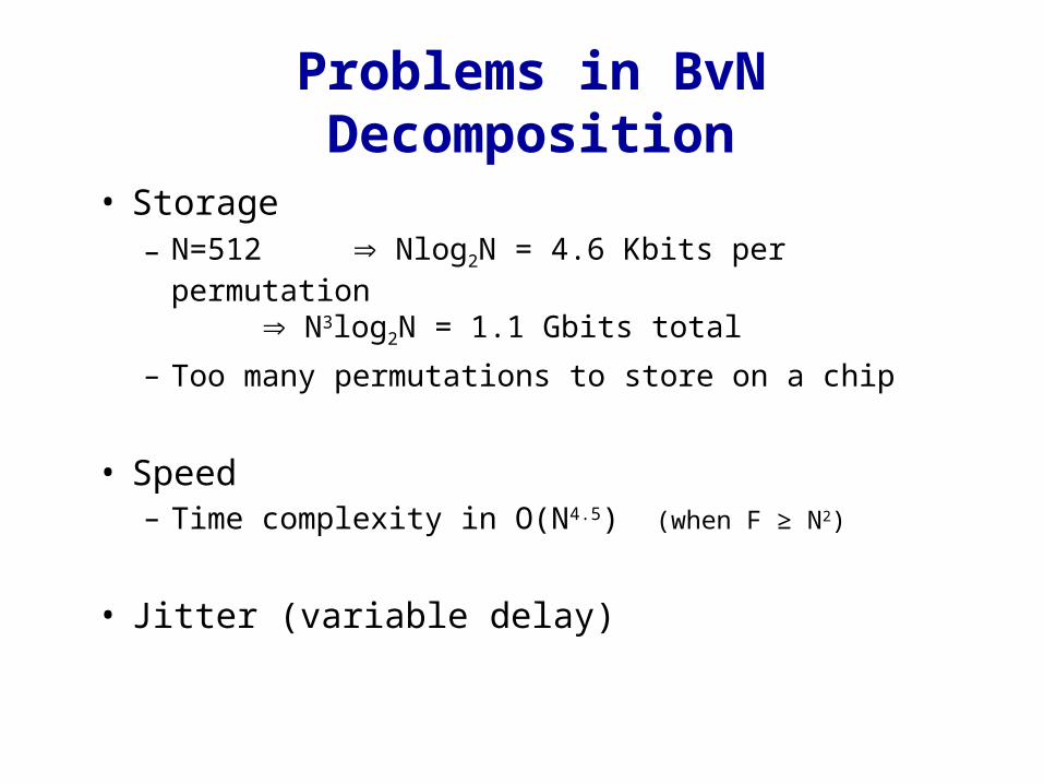
Problems in BvN Decomposition

• Storage– N=512 Nlog2N = 4.6 Kbits per permutation

N3log2N = 1.1 Gbits total

– Too many permutations to store on a chip

• Speed– Time complexity in O(N4.5) (when F ≥ N2)

• Jitter (variable delay)

What is jitter?

...,,...,, ,,...,, schedule 1

100

50

222

50

111 MMMMMMM

• BvN (naive implementation):

• Smooth scheduling (low-jitter):

21

100

1

2

1

1

1

2

1

1

1

2

1

1 ,,,,...,,,, schedule MMMMMMMM

1 2

50 5050 50

50 50R M M

01

10M ,

10

01M where 21

Why smooth scheduling?

• Low-jitter guaranteed-bandwidth traffic– For instance Expedited Forwarding in Diffserv– Typically, 10% of the traffic

• Less burstiness– Bursty TCP traffic results in multiple losses

• Increased short-term fairness

• Less buffering (or delay lines) for smoothly arriving flows

Outline

1. Frame Scheduling

2. GLJD Algorithm

3. GLJD Guarantees

4. Simulations

5. Conclusion

Smooth scheduling idea

1. Decomposition: find a decomposition of R into matches such that each entry of R appears in at most one match.

2. Scheduling: use a scheduling algorithm to smoothly schedule the matches (matches are independent).

1,1

,

1

K

k

jik

K

kkk MMR Our

algorithm

Known method

Smooth scheduling example

1. Decomposition:

2. Scheduling:

121

112

211

R

321

100

010

001

1

001

100

010

1

010

001

100

2

MMM

R

,...,,,,,,, 31213121 MMMMMMMM

100

001

010

010

100

001

001

010

100

010

001

100

R

Note: BvN could yield:

Optimal Smooth Decomposition

Theorem: Optimal decomposition is NP-hard Need to find a provably good approximation algorithm

1

1

, , ,

1 1

k

Find optimal D = min (cycle time) = min

s.t.: Decomposition: ,

is a match: 1, 1, {0,1}

Each element (i,j ) is in at most one match M :

K

kk

K

k kk

N Ni j i j i j

k k k ki j

R M

M M M M

,

1

1K

i jk

k

M

Formal Problem:

Smooth Decomposition Example

100) BvN100 (sum

2242351

3314530

5602411

4022038

R

1 0 0 0 0 0 0 1 0 0 1 0 0 1 0 0

0 1 0 0 1 0 0 0 0 0 0 1 0 0 1 0 38 53 23 60

0 0 1 0 0 1 0 0 1Diagonal

0 0 0 0 0 0 1

0 0 0 1 0 0 1 0 0 1 0 0 1 0 0 0

(Bandwidth: 38 53 23 60 174 1

s:

00 BvN)

R

0 0 0 1 1 0 0 0 0 0 1 0 0 0 0 0

0 0 1 0 0 1 0 0 1 0 0 0 0 0 0 1 60 38 33 5

0 1 0 0 0 0 1 0 0 0Optima

0 1 0 0 0 0

1 0 0 0 0 0 0 1 0 1 0 0 0 0 1 0

(Bandwidth: D = 60 38 33 5 136 100 BvN)

l D: R

Idea: group together close coefficients

GLJD (Greedy Low-Jitter Decomposition)

100) (sum

2242351

3314530

5602411

4022038

R

0 0 0 1 1 0 0 0 0 0 1 0 0 0 0 0 0 0 0 0

0 0 1 0 0 1 0 0 1 0 0 0 0 0 0 0 0 0 0 160 38 22 22 5

0 1 0 0 0 0 0 1 0 0 0 0 0 0 1 0 0 0 0 0

1 0 0 0 0 0 1 0 0 1 0 0 0 0 0 1 0 0 0 0

(Bandwidth: 60 38 22 22 5 147 : more tha

R

n D=136 optimal and 100 BvN, less than 174 diagonals)

Outline

1. Frame Scheduling

2. GLJD Algorithm

3. GLJD Guarantees

4. Simulations

5. Conclusion

Theorem 1 (matrices): GLJD needs at most K=2N-1 matrices

Proof outline: Consider the union of a row i and a column j. It has at most 2N-1 non-zero elements. At each iteration, at least one of these elements is scheduled and removed from further consideration.

GLJD guarantees

Theorem 2 (upper bound): Assume R of sum 1. Both D and GLJD need a bandwidth 2HN-1, i.e. O(ln N)

Proof outline: upper-bound each matrix weight and sum the bounds

Theorem 3 (lower bound): Both D and GLJD need a bandwidth of (ln N)

Proof outline: use a specific matrix as a counter-example

GLJD guarantees

Theorem 4 (approximation ratio): GLJD is a (2-1/N) bandwidth approximation algorithm to D

Proof outline: upper-bound bandwidth needed by GLJD and lower-bound D based on matrix structure

GLJD guarantees

Outline

1. Frame Scheduling

2. GLJD Algorithm

3. GLJD Guarantees

4. Simulations

5. Conclusion

GLJD Simulation Summary (N=64)

• Gain with respect to BvN:– Smoothness– Storage

• GLJD needs 10 times less matrices than BvN– Complexity:

• GLJD is 100 times faster than BvN

• Trade-off with:– Bandwidth Efficiency

• Bandwidth ratio guarantee = 2HN-1 = 8.5• Simulation ~ 1.55

Simulations: jitter

Conclusion

• BvN decomposition is an optimal but impractical algorithm

• Practical smooth decomposition with – Lower storage requirements– Lower complexity (ln N) bandwidth approximation ratio

guarantee