Growth and Pollution Convergence: Theory and

Evidence

C. Ordás Criado∗ † ‡ S. Valente§ T. Stengos¶

Final version: March 14, 2011

Running title: Growth and Pollution Convergence

∗Corresponding author. Email: cordas@ethz.ch; fax: +41 44 632 1622.†ETH Zurich, Center for Energy Policy and Economics (CEPE), 8032 Zurich, Switzerland.‡Université Laval, Département d’économique, G1V0A6, Québec, Canada.§ETH Zurich, Center of Economic Research (CER), 8032 Zurich, Switzerland.¶University of Guelph, Department of Economics, N1G2W1, Ontario, Canada.

1

Growth and Pollution Convergence:Theory and Evidence

Abstract

Stabilizing pollution levels in the long run is a pre-requisite for sustainable growth. We

develop a neoclassical growth model with endogenous emission reduction predicting

that, along optimal sustainable paths, pollution growth rates are (i) positively related

to output growth (scale effect) and (ii) negatively related to emission levels (defensive

effect). This dynamic law reduces to a convergence equation that is empirically tested

for two major and regulated air pollutants - sulfur oxides and nitrogen oxides - with a

panel of 25 European countries spanning the years 1980-2005. Traditional parametric

models are rejected by the data. More flexible regression techniques confirm the exis-

tence of both the scale and the defensive effect, supporting the model predictions.

JEL Classification numbers: C14, C23, O13, Q53

Key Words: Air pollution, convergence, economic growth, nonparametric regres-

sions.

2

1 Introduction

Making economic growth compatible with environmental preservation in the long run is

a major challenge facing modern societies. The economic literature tackles this issue by

analyzing the conditions under which an economy may achieve sustainable growth – that

is, balanced growth paths characterized by growing per capita incomes and non-declining

environmental quality (Brock and Taylor, 2005). In this framework, sustainability requires

satisfying a general condition of pollution convergence: pollution must be bounded in the

long run and approach a finite steady state level despite positive growth in GDP per capita.

A more specific question is: how do pollution dynamics interact with output dynamics along

sustainable growth paths? In this paper, we tackle this issue at both the theoretical and the

empirical level. First, considering a growth model with endogenous pollution abatement,

we show that the optimal path is characterized by a precise dynamic relationship between

pollution growth rates, emission levels, and output growth rates, which induces pollution

convergence in the long run. Second, we test this dynamic law empirically for two major air

pollutants, using panel data from European countries.

Our analysis is based on a neoclassical growth model where pollution generated by the

production process reduces private welfare. In this framework, sustainable growth requires

the use of more efficient technologies as well as defensive expenditures to curb emissions

(Van der Ploeg and Withagen, 1991; Bovenberg and Smulders, 1995; Brock and Taylor, 2010).

We analyze the optimal path of an economy in which purposeful investment in clean technolo-

gies generates positive feedback effects on environmental quality: output growth is driven by

capital accumulation and labor-augmenting technological progress whereas pollution growth

is contrasted by emission-reducing technical change. Differently from Brock and Taylor

(2010), we assume that both the propensities to consume and to invest in clean technologies

are endogenously determined by utility maximization. We show that pollution stabilization

in the long run is associated with a precise law: during the whole transition, the growth

3

rate of emissions per capita is (i) negatively related to the level of emissions per capita and

(ii) positively related to the growth rate of output per capita. Result (i) is called ‘defensive

effect’, and reflects the effectiveness of abatement expenditures in limiting pollution growth.

Result (ii) is a ‘scale effect’ implied by the positive relation between output and emission

levels. By virtue of the defensive effect, pollution growth rates regress to zero and emissions

per capita are bounded in the long run. The dynamic law derived in the theoretical model

may be interpreted as a β-convergence equation, i.e., an intertemporal relation predicting

an inverse relationship between the growth rate of the variable of interest (pollution, in our

case) and its past level.

The notion of β-convergence is widely used in the growth literature, where the variable

of interest is per capita income. Indeed, the neoclassical growth model predicts an inverse

relationship between output levels and growth rates during the transition to the long run

equilibrium. Accordingly, the empirical literature tests whether this prediction is observed

across countries. Early studies focused on absolute β-convergence, i.e., the hypothesis that

the negative growth-level relationship is characterized by the same parameters across the

different economies considered in the sample1. More recent studies allow for structural het-

erogeneities among countries and test for conditional β-convergence, i.e., check the existence

of a negative growth-level relationship in incomes after controlling for the effects of other

determinants of the growth dynamics (Barro and Sala-i-Martin, 2004). In the present paper,

we study pollution dynamics in a similar fashion but with an additional element: our model

predicts not only a negative growth-level relationship in the variable of interest "pollution",

but also a positive interaction between pollution growth and income growth. Our empirical

analysis can thus be considered a convergence test in which β-convergence in pollution is

conditional on country-specific output dynamics.1The hypothesis of absolute beta-convergence seems to hold within selected groups of industrialized

economies - namely, OECD countries in the post-war period - but it does not hold if the country sample isextended to include non-OECD economies: see, e.g., Acemoglu (2009).

4

We empirically test the existence of both the scale and the defensive effect for two major

air pollutants, sulfur oxides (SOX) and nitrogen oxides (NOX), using panel data for 25

Eastern and Western European countries over the period 1980-2005. We consider different

regression methods. The standard parametric approach confirms the existence of these effects

for both pollutants but the linear models are rejected by the data. We address this issue by

exploiting more flexible approaches - i.e., semi-parametric and nonparametric regressions -

that better capture nonlinearities and heterogeneities across Eastern and Western European

countries. Our results are consistent with the predictions of the theoretical model and confirm

the existence of scale effects and defensive effects for SOX and NOX.

Our analysis differs from the previous literature on pollution dynamics in several respects.

Most studies examine alternative notions of pollution convergence. A first body of contribu-

tions analyses stochastic convergence, that is, the time-series properties of pollution differ-

entials between countries or regions. List (1999) and Bulte et al. (2007) find stationary gaps

across the US states for NOX and SO2 emissions per capita especially since the start of the

federal regulation period in the 1970s; the results of Nguyen Van (2005) and Aldy (2006) show

worldwide divergence for CO2 emissions per capita since the 1960s, while Strazicich and List

(2003) and Romero-Ávila (2008) obtain convergence among OECD countries over the same

period. A second approach is followed by Aldy (2006), who analyses σ-convergence – i.e.,

the evolution of simple dispersion measures over time – and confirms the above results for

CO2. A third notion of convergence, proposed by Quah (1993a), focuses on distributional

dynamics2 and examines the evolution of the spatial distribution of pollution levels over

time. In this framework, Nguyen Van (2005), Aldy (2006) and Ordás Criado and Grether

(forthcoming) reject the existence of polarization phenomena across countries except within

the OECD and European areas.

Before our paper, the notion of pollution β-convergence has been analyzed in List (1999)2This method is also referred to as Markov transition matrices or ‘stochastic kernels’.

5

for NOX and SO2, and in Strazicich and List (2003), Nguyen Van (2005) and Brock and Taylor

(2010) for CO2 emissions per capita. These authors test the slope of a log-linear relation

between pollution growth and pollution levels and obtain a negative coefficient. Differently

from these contributions, (i) we estimate a reduced-form equation derived from the optimal-

ity conditions of a dynamic model, (ii) we explicitly test for misspecification and employ

nonparametric methods, and (iii) we consider NOX and SOX emissions at the European

level. In particular, the choice of analyzing SOX and NOX is linked to the assumptions of

the theoretical model, in which environmental quality is preserved through defensive expen-

ditures, and pollution is represented as a local welfare-reducing flow.

As noted by Friedman (1992), Quah (1993b) and Evans and Karras (1996), among oth-

ers, beta-convergence in income does not formally imply decreasing gaps in income across

countries over time, nor it does guarantee stationarity for the income levels of the countries

included in the sample. In line with these considerations, our results do not represent an

estimate of the speed of convergence in pollution across countries, but rather an empirical

test of the existence of the defensive effect – a necessary condition for sustainability in the

long run.

2 A model of growth and optimal emission reduction

The relationships between economic growth and pollution dynamics are investigated by a

growing body of theoretical literature. In the traditional approach – pioneered by Keeler et al.

(1971), and extended by Van der Ploeg and Withagen (1991) and Bovenberg and Smulders

(1995), amongst others - pollution is positively related to output levels according to an emis-

sion function representing the environmental damage caused by the production process. If

the emission intensity is fixed, pollution increases linearly with production. However, if the

economy invests resources in the development of cleaner technologies, the elasticity of emis-

sions to output is reduced over time and economic growth induces positive feedback effects

6

on environmental quality. This mechanism is emphasized by Brock and Taylor (2010) in a

‘Green Solow Model’ – i.e., a neoclassical growth model in which the economy spends fixed

fractions of income in capital investment and in pollution-abatement activities – in which

pollution converges to a finite steady state if the rate of emission-reducing technological

progress is sufficiently high3.

In this section, we build a model of optimal emission reduction that allows us to study

the interactions between pollution convergence and capital accumulation in a more specific

context. Differently from Brock and Taylor (2010), we assume that both the saving rate and

the propensity to spend in abatement are endogenously determined by utility maximization.

This allows us to derive the basic equation to be employed in the empirical analysis from the

optimality conditions of a centralized social problem: the saddle path followed by the econ-

omy determines a precise dynamic relationship between pollution growth, pollution levels,

and income growth rates, that can be tested using regression methods.

At the conceptual level, the difference with Brock and Taylor (2010) is twofold. First,

the equation describing pollution convergence over time is explicitly micro-founded. Second,

because we assume optimal control of the pollution flow at the economy level, our frame-

work is particularly suited for applications to local air pollutants – e.g., NOX and SOX –

but not to CO2, which is the pollutant examined in most related literature. At the for-

mal level, our model shares the general features of Ramsey-Cass-Koopmans models with

welfare-reducing emissions. Van der Ploeg and Withagen (1991) study several variants of

this framework in the absence of technological progress - they consider, in particular, a ‘flow-

pollution model’ where emission-reducing investment is excluded, and a ‘clean-technologies

model’ where abatement is optimized but there is no capital accumulation. Our model can be

interpreted either as an extension of the ‘flow-pollution model’ to include optimal investment3The aim of Brock and Taylor (2010) is primarily to rationalize the existence of an Environmental Kuznets

Curve (EKC) in a simple theoretical framework including capital accumulation and emission abatement.They exploit the work of Mankiw, Romer and Weil (1992) to derive a convergence equation for pollution.

7

in emission reduction, or equivalently, as an extension of the ‘clean-technologies model’ to

include capital accumulation. In both cases, the value added of our analysis is the derivation

of the joint dynamics of pollution, capital and output in an environment where the paths

of these variables are optimally chosen and there are positive rates of labor-augmenting and

emission-reducing technological progress.

2.1 The Ramsey setting

As our empirical analysis will focus on the dynamics of emissions per capita, we will treat

pollution as a flow-variable that affects private utility in per capita terms. The model

economy is characterized by the following assumptions:

Y (t) = F (K (t) , B (t)N (t)) , B (t) = B0eπt, N (t) = N0e

nt, (1)

K (t) = Y (t)− C (t)−X (t)− δK (t) , (2)

P (t) = τ (t)Y (t) , (3)

U (t) = U (c (t) , p (t)) , Uc > 0, Ucc ≤ 0, Up < 0, Upp < 0, (4)

where t ∈ [0,∞) is the time index.4 Technology (1) assumes that aggregate output, Y ,

is produced by means of capital, K, and efficient labor, BN , according to a linearly ho-

mogeneous production function F (., .) displaying positive and strictly decreasing marginal

productivities in both factors and satisfying the Inada conditions. Population N grows at the

exogenous rate n > 0, and labor efficiency B grows at the given rate of labor-augmenting

technical progress π > 0. Expression (2) is the accumulation constraint, where δ ≥ 0 is

the rate of physical depreciation of capital: net investment equals output minus the sum

of consumption, C, and defensive expenditures, X. By defensive expenditures we mean re-

sources devoted to activities that reduce the emission intensity of the production sector –4Using standard notation, we define Z ≡ dZ/dt as the time-derivative of the generic variable Z (t), and

GQ ≡ ∂G/∂Q and GQQ ≡ ∂2G/∂Q2 as the partial derivatives of the generic function G (Q).

8

henceforth called ICT (investment in cleaner technology). The pollution function (3) asserts

that aggregate emissions per unit of time, P , are proportional to aggregate output, and τ

is the global emission intensity. Expression (4) defines private utility, U , as a function of

consumption per capita, c ≡ C/N , and emissions per capita, p ≡ P/N , where Up < 0 and

Upp < 0 guarantee that the disutility from pollution is convex.

In order to obtain a full characterization of the optimal dynamics, we model (i) the

process of emission reduction and (ii) the trade-off between consumption and environmental

quality by means of two specifications often exploited in the literature. First, following

Brock and Taylor (2010), we assume that the aggregate emission intensity is given by

τ (t) ≡ Ω (t) ·[1− X (t)

Y (t)

]ε, ε > 1, (5)

where Ω (t) is the baseline emission intensity, and the second term is a function represent-

ing the effects of ICT. The share of output devoted to defensive expenditures, X/Y , will

be called ICT effort, and corresponds to the propensity to invest in cleaner technologies,

bounded between zero and unity. From (5), maximal ICT effort, X = Y , implies zero

emissions whereas zero defensive expenditures, X = 0, imply that the emission intensity

equals the baseline level. Also the baseline intensity varies over time as it is influenced by

technological progress. As shown by Brock and Taylor (2010), explosive dynamics in pol-

lution per capita can be avoided only if the rate of emission-reducing progress – i.e., the

effects of technical improvements that reduce Ω (t) over time – is at least equal to the rate

of output-augmenting technical progress. In the present model, this sustainability condition

corresponds to Ω (t) /Ω (t) ≤ −π. In order to ensure that stabilizing per capita emissions

in the long run is technically feasible, we assume symmetric rates of emission-reducing and

labor-augmenting progress by setting Ω (t) = Ω0e−πt. Alternative assumptions that sat-

isfy the sustainability condition – e.g., Ω (t) = Ω0e−ωt with ω > π – would complicate the

analysis of steady-state equilibria without affecting the main results concerning pollution

9

convergence.5

The second assumption is related to private preferences. In this respect, we specify a

utility function that allows us to characterize optimal dynamics analytically:

U (c (t) , p (t)) = σ ln c (t)− ςp (t)θ , θ > 1, (6)

where σ > 0 and ς > 0 are the weights on utility from consumption and disutility from

pollution, respectively. Function (6) satisfies all the properties listed in (4), consistently

with the conditions for a well-behaved problem – see Van der Ploeg and Withagen (1991).

In particular, θ > 1 ensures that the marginal damage from emissions is increasing.

As noted before, the distinguishing feature of our analysis is that we assume both the

consumption and the ICT time paths to be chosen optimally. Denoting by ρ > 0 the social

discount rate, the optimal path is defined as a sequence of consumption levels and defensive

expenditures maximizing present-value welfare

∫ ∞

0

U (c (t) , p (t)) e−ρtdt, (7)

subject to the accumulation constraint (2), the pollution function (3), and the non-negativity

constraint K (t) ≥ 0 in each t for a given initial stock K (0) = K0. This problem can be

solved more easily by denoting ICT effort as

χ (t) ≡ X (t) /Y (t) ,

and normalizing the relevant variables in terms of labor-efficiency units. Setting y ≡ Y/ (BN)

5Assuming more intense emission-reducing technical progress, Ω/Ω = −ω < −π, would not affect themain results: pollution per capita would tend to a particular steady-state level (i.e., zero) in the long run.We assume symmetric rates of emission-reducing and labor-augmenting progress because asymmetric rateswould imply additional technical difficulties without any gain for the present analysis. This point is clarifiedin an Appendix available at JEEM’s online archive of supplementary material, which can be accessed athttp://aere.org/journals/.

10

and k ≡ K/ (BN), the homogeneous production function in (1) yields the intensive form y =

f (k) = F (k, 1), where fk coincides with the marginal product of capital. As a consequence,

equations (2)-(3) can be written as

k (t) = f (k (t)) [1− χ (t)]− c (t)− (δ + n+ π) k (t) , (8)

p (t) = Ω (t) [1− χ (t)]ε f (k (t)) , (9)

where c ≡ C/ (BN) and p ≡ P/ (BN) are ‘normalized’ consumption and pollution, respec-

tively. The arguments in the utility function respectively equal c = cB and p = pB, and the

optimal path can be found by maximizing (7) subject to (8)-(9), using c (t), p (t) and χ (t) as

control variables. As shown in the Appendix, the necessary conditions for optimality yield

c (t) /c (t) =[fk (t) (1− χ (t))

(1− ε−1

)]− (ρ+ δ + n+ π) , (10)

1− χ (t) = Γf (k (t))−θ−1εθ−1 c (t)−

1εθ−1 , (11)

where Γ > 0 is an exogenous constant, and fk (t) ≡ fk (k (t)). Expression (10) is the growth

rate of normalized consumption along the optimal path, which is different from the usual

Keynes-Ramsey rule due to the presence of abatement effort, χ (t), and of the elasticity factor

1− ε−1 that quantifies the distortion in the marginal benefit from accumulation induced by

welfare-reducing emissions.6 Condition (11) determines the optimal propensity to spend in

abatement, which exhibits a precise link with the time-paths of k (t) and c (t): if consumption

and output increase (decrease) along the optimal path, the abatement effort χ (t) increases

(decreases) as well. The dynamic properties of the optimal path can be analyzed as follows.6In general, the Keynes-Ramsey rule asserts that the consumption growth rate is proportional to the

difference between the marginal benefit from capital accumulation and the utility discount rate. In theneoclassical model without pollution, the marginal benefit from accumulation equals the marginal productof capital net of depreciation; in the current model, instead, it equals the term in square brackets in (10),which is strictly lower than fk. The reason is that the optimal path takes into account the fact that highercapital implies ceteris paribus higher pollution, which induces a wedge between capital productivity andutility-benefits from accumulation.

11

Omitting time-arguments for simplicity, define the right hand side of (11) as a function

Φ (k, c) ≡ Γf (k)−θ−1εθ−1 c−

1εθ−1 , (12)

where Φk < 0 and Φc < 0. Substituting 1 − χ = Φ(k, c) in (8) and (10), the resulting

dynamic system is

k = f (k) Φ (k, c)− c− (ρ− ρ) k, (13)

c = fk (k) Φ (k, c)(1− ε−1

)c− ρc, (14)

where we have defined ρ ≡ ρ + δ + n + π. We denote by (css, kss) the couple of values

representing the simultaneous steady-state equilibrium of system (13)-(14). It can be shown

that the steady state exists and is unique for any well-behaved neoclassical production func-

tion7. Also the stability properties of the steady state are quite general and do not require

assuming specific technologies:

Lemma 1 The simultaneous steady-state equilibrium (css, kss) of system (13)-(14) is saddle-

point stable. Given the initial condition k (0) = k0, the optimal path is unique and implies

convergence towards (css, kss).

Lemma 1 has three main implications. First, convergence towards (css, kss) implies that

the propensity to spend in clean technologies and the marginal product of capital are constant

in the long run. The asymptotic value of ICT effort, χss, is determined by condition (11).

Imposing stationarity in (10), we obtain the long-run level of the marginal product of capital

f ssk =

ρ+ δ + n + π

(1− χss) (1− ε−1). (15)

Expression (15) implies that normalized capital kss will be lower than in the Ramsey model7A proof of the existence and uniqueness is available at the online archive.

12

- where the modified golden rule f ssk = ρ + δ + n + π holds.8 The second implication of

Lemma 1 is that the economy displays balanced growth in the long run. Both c = C/NB

and k = K/NB, as well as ICT effort χ = X/Y , achieve stationary values. Hence, aggregate

output, capital, and expenditures grow asymptotically at the same balanced rate

limt→∞

Y (t)

Y (t)= lim

t→∞K (t)

K (t)= lim

t→∞C (t)

C (t)= lim

t→∞X (t)

X (t)= n+ π. (16)

Result (16) implies that, in the long run, per capita variables grow at the rate of labor-

augmenting technical progress, π. The third implication of Lemma 1 is that pollution per

capita, p (t) = p (t)B (t), converges to a constant steady-state level. From (3) and (1), the

dynamics of p (t) are governed by

p (t) = Ω (t) Φ (k (t) , c (t))ε f (k (t))B (t) = Ω0B0Γεf (k (t))

ε−1εθ−1 c (t)−

εεθ−1 , (17)

which implies

limt→∞

p (t) = pss ≡ Ω0B0Γεf (kss)

ε−1εθ−1 (css)−

εεθ−1 . (18)

The transitional dynamics of pollution per capita can be studied by re-introducing p (t) in

the dynamic system (13)-(14). In fact, pollution per capita and consumption are two jump

variables linked by an optimality relation: using (17), we can transform system (13)-(14) into

an equivalent system describing the joint dynamics of k (t) and p (t). As the dynamics of

(k (t) , c (t)) are saddle-point stable, we expect the same behavior to arise in the (k (t) , p (t))

plane. This result is formally proved below. In order to obtain an explicit relation between

pollution per capita and other endogenous variables of empirical interest, we henceforth

assume that the aggregate technology is Cobb-Douglas.8As the planner takes into account the fact that higher capital implies ceteris paribus higher pollution, it

is optimal to accumulate less capital with respect to the modified golden rule in the long run (see Van derPloeg and Withagen, 1991).

13

2.2 Transitional dynamics of pollution per capita

Suppose that technology (1) takes the Cobb-Douglas form Y = Kα (BN)1−α, and write

normalized output f (k) = kα, where α ∈ (0, 1). In this case, the dynamics of pollution per

capita and normalized capital are governed by the non-linear system (see Appendix A)

g (p (t)) = ϕ0 − ϕ1k (t)α−1−α

ε p (t)−(θ−1ε) , (19)

g (k (t)) = ϕ2k (t)−(1−α+α

ε) p (t)

1ε

(1− ϕ3p (t)

−θ)− ϕ4, (20)

where g (p (t)) ≡ (dp (t) /dt) /p (t) and g (k (t)) ≡ k (t) /k (t) are instantaneous growth rates

and (ϕ0, ϕ1, ϕ2, ϕ3, ϕ4) are exogenous constants, all strictly positive. From (19)-(20), the

stationary loci read

g (p (t)) = 0 → k (t) =

[ϕ1

ϕ0p (t)−(θ−

1ε)] 1

1−α+αε

, (21)

g (k (t)) = 0 → k (t) =

[ϕ2

ϕ4p (t)

1ε

(1− ϕ3p (t)

−θ)] 1

1−α+αε

, (22)

where locus (21) is strictly decreasing and (22) is strictly increasing in the (k (t) , p (t)) plane.

Equations (19) and (20) respectively imply ∂g (p) /∂p > 0 and ∂g (k) /∂k < 0 and thereby the

phase diagram reported in Figure 1. The simultaneous steady-state (kss, pss) is saddle-point

stable. In particular, given an initial stock k (0) = k0, the associated initial level of pollution

per capita p (0) lies along a saddle path that is strictly decreasing in the (k (t) , p (t)) plane.

If we want to reproduce the dynamics of an economy exhibiting positive accumulation during

the transition, we must assume k0 < kss. In this case, the strictly-decreasing saddle path

implies that the initial level of pollution per capita is above the long-run value, p (0) > pss.

Hence, the transitional dynamics are characterized by a decreasing time path of pollution per

capita, as shown in Figure 1. These results can be formally proved by linearizing system

14

(19)-(20); see the Appendix for details. This gives

g (p (t)) ≈ m1 (p (t)− pss) +m2 (k (t)− kss) , (23)

g (k (t)) ≈ m3 (p (t)− pss) +m4 (k (t)− kss) , (24)

where the coefficients are m1, m2, m3 > 0 and m4 < 0. The Jacobian matrix associated with

(23)-(24) confirms saddle-point stability and, in particular, yields the equation of the stable

arm

(k (t)− kss) = φ (p (t)− pss) , φ < 0, (25)

where φ < 0 implies a negatively-sloped saddle path. The stable-arm equation allows us to

obtain an explicit relation between pollution per capita growth and the other endogenous

variables of empirical interest. In fact, substituting (25) in (23), and using (24) to eliminate

normalized capital k (t) from the resulting expression, we obtain

g (p (t)) ≈ m1

α (m3 +m4φ)(g (y (t))− π) + φm2 (p (t)− pss) , (26)

where g (y (t)) is the growth rate of output per capita y (t). Collecting the constant terms

and checking the signs of the exogenous parameters appearing in (26), we obtain

Proposition 2 Along the optimal path, the instantaneous growth rate of emissions per capita

is (i) positively related to the growth rate of output per capita and (ii) negatively related to

the level of emissions per capita:

g (p (t)) ≈ H0 +H1g (y (t))−H2p (t) , (27)

where H1 > 0 and H2 > 0.

15

Proposition 2 emphasizes the main prediction of our model: along the optimal path,

pollution levels obey a precise dynamic relationship. First, the growth rate of emissions per

capita is positively related to the growth rate of output per capita: this is a ‘scale effect’

implied by the positive relation between output and emission levels. Second, the growth rate

of emissions per capita is negatively related to the level of emissions per capita: we label

this a ‘defensive effect’ as it reflects the effectiveness of abatement expenditures in limiting

pollution growth9. The difference with the reduced forms of Solow-type models employed,

e.g., in Brock and Taylor (2010) and Bulte et al. (2007), is that (27) incorporates all the

optimality conditions governing consumption and investment decisions.

It is worth stressing that result (27) can be interpreted as an equation predicting β-

convergence in pollution: the defensive effect determines a negative relationship between

pollution growth and pollution levels. This notion of β-convergence is however conditional

on the existence of the scale effect, the positive relation between pollution growth and output

growth. In the remainder of this paper, our aim is to verify whether the existence of both

the defensive and the scale effects receives empirical support. In this respect, equation (27)

suggests considering a model equation like

GPt = γ0 − β logPt−T + γ1GYt, (28)

where (GPt, GYt, Pt−T ) represent (g (p (t)) , g (y (t)) , p (t)) in a discrete-time setting with T -

year periods growth rates, and testing empirically whether the coefficients β and γ1 are

strictly positive. An extended version of (28) is

GPt = γ0 − β logPt−T + γ1GYt + γ2 log Yt−T , (29)9Our definition of defensive effects may include – but is not limited to – the technique effect typically

mentioned in the literature, e.g. Brock and Taylor (2010, eq.6), because it captures, in addition to the rateof emission-reducing technical progress, all the endogenous effects that contrast pollution growth over time- e.g., variations in the propensity to invest in clean technologies - after controlling for the effect of outputgrowth.

16

which includes initial levels of output per capita, Yt−T , as an additional explanatory variable.

The reason for considering the extended version (29) is that (28) is directly obtained from a

first-order approximation of the saddle path. The deviations arising between the exact non-

linear saddle path in Figure 1 and the linearized saddle path (25) are essentially due to the

dynamics of capital per efficient labor: in order to capture these high order effects cleaned

out by the Taylor expansions (23)-(24), the natural hypothesis is to include the initial level

of output per capita as an additional regressor without postulating a priori a definite sign

for coefficient γ2.

3 Empirical methodology

This section proposes an empirical methodology which investigates the existence of scale

effects and defensive effects by testing equations (28) and (29). As is common in recent

economic growth papers, the predictions of the theoretical model are explored with panel

regressions. Our panel estimates are based on four 5-year periods starting in year t =

{1980, 1985, 1990, 1995, 2000}. As pointed out by Barro and Sala-i-Martin (2004), taking

shorter periods carries the risk of missing long run adjustments. More precisely, short run

growth rates tend to capture short term adjustments around the trend rather than long run

convergence. In the presence of business cycles, this leads to an upward bias of the estimates

of the convergence speed – see Shioji (1997).

We consider three regression approaches: parametric, semiparametric and fully non-

parametric. All these specifications allow for structural dissimilarities within groupings of

countries through a group-specific dichotomous variable. Time dummies are also included to

account for potential structural breaks and to capture time-specific effects in the relationship.

Parametric model. The panel regression is given by

GPi,t = α1 + α2Di + α3,tDt + β logPi,t−T + γ1GYi,t + γ2 log Yi,t−T + εi,t (30)

17

where GPi,t is the growth rate of emissions per capita in the i-th country, measured by the

average log changes (1/T )log(Pi,t/Pi,t−T ) over the time span t−T to t; Di is a dummy equal

to 1 if the i-th country is an EU15 member and equal to 0 if not; Dt are dummy variables

for each period t of the panel; Pi,t−T is the level of emissions per capita (tons/capita) in

the i-th country at time t − T ; Yi,t−T is the level of GDP per capita (in 1990 International

Geary-Khamis dollars) in the i-th country at time t−T ; GYi,t is the growth rate of GDP per

capita in the i-th country, measured by the average log changes (1/T )log(Yi,t/Yi,t−T ) over

the time span t − T to t; εi,t is an iid error term. Model (30) encompasses the two test-

equations proposed in the previous section: if we impose γ2 = 0 , the regression corresponds

to a stochastic version of equation (28), while estimating the full regression amounts to

testing equation (29). Model (30) can be naturally estimated either with cross-sectional or

panel regressions10. The latter framework has the advantage of better capturing unobserved

heterogeneity and nonlinearities in the relationship.

Given the potential feedback effect of pollution on GDP, the regression’s coefficients can

suffer from endogeneity bias. We address this issue by providing Instrumental Variables

(henceforth, IV) estimates. Following Barro and Sala-i-Martin (2004), we keep the first 5-

year period starting in 1980 out of the sample to build instruments. Therefore, IV versions

of the panel regressions are proposed with Yi,(t−1)−T as instrument for Yi,t−T and GYi,t−1 for

GYi,t.

Two fundamental hypotheses are tested regarding the OLS specifications. The null of

homoscedasticity is checked with a robust version of the Breusch-Pagan LM heteroscedas-

ticity test (Greene, 2008). We also apply the misspecification test of Hsiao et al. (2007) to

check if the parametric linear models provide consistent estimates. This test contrasts the

following two hypotheses: H0 : E(yi, xi) = E(yi, xi;ϕ) vs. H1 : E(yi, xi) = E(yi, xi;ϕ). If10When T is set to the entire length of the time dimension, we can drop the dummies and specification

(30) becomes a cross-sectional model where the dynamic component is captured by growth rates over thewhole period.

18

H0 is not accepted, more flexible specifications can be explored. This paper considers two

alternatives to the linear parametric model (30) that we present below.

Semiparametric model. Our second specification is a semiparametric additive model

which gives full flexibility to the continuous explanatory components. The dummy variables

enter the equation parametrically whereas the other regressors enter nonparametrically with

a separable structure. This is the partially linear (PLR) additively separable regression

model which can be written as

GPi,t = α1 + α2Di + α3,tDt +

3∑j=1

fj(xcj) + εi,t (31)

where fj(xcj) are three unknown nonlinear functions, one for each j-th continuous factor

in (30), that is, xc1 = logPi,t−T , xc

2 = GYi,t, xc3 = log Yi,t−T . The first three terms in

specification (31) constitute the linear part of the PLR model while the last term∑3

j=1 fj(xcj)

is the additive nonparametric component. Compared to the parametric model (30), the

PLR setting imposes no restriction on the flexibility of the additive nonparametric factors

and has a straightforward graphical representation. The additive block is a special case

of the general smooth function f(xc1, x

c2, x

c3), which can be estimated more efficiently than

a fully nonparametric setting when it represents the true relationship. Several approaches

provide consistent fits of PLR models. Here we employ the procedure of Wood (2006) which

decomposes the flexible additive components into a finite sum of spline terms and controls for

the smoothness of the functions with cross-validation. The results are reported graphically

for each estimated function fj(xcj), with j = 1, 2, 3.

Fully nonparametric model. We relax the functional restrictions in the parametric model

(30) and the nonparametric additive hypothesis of the PLR equation (31) by estimating

a nonparametric regression which allows all kind of interactions between the independent

variables (in particular between the continuous regressors and the dummy variables). This

19

fully flexible specification is given by

GPi,t = f(xd,xc) + εi,t (32)

where xd = [Di, Dt] are the usual discrete regressors (but with Dt defined as a single discrete

trend factor) and xc = [logPi,t−T , GYi,t, log Yi,t−T ] are the continuous explanatory factors.

We estimate (32) using the new kernel method proposed by Racine and Li (2004). This

estimator allows us to compute nonparametric regressions with mixed independent variables

(i.e., discrete and continuous regressors) and is consistent in panels with a small time di-

mension t relative to the individual dimension11 i. We use least squares cross-validation in

conjunction with a locally linear kernel estimator to determine the bandwidths: this allows

us to correct for potential bias near the support’s boundaries and to discriminate between

linear and nonlinear regressors12.

Graphical representations. The relationship between the continuous predictors and the

response in non or semiparametric regressions is usually reported graphically. We show the

results for specifications (31) and (32) with partial regression plots. In that respect, we follow

Maasoumi et al. (2007): we present the nonparametric regression of GPi,t on the continuous

regressors xc for EU15 countries (Di = 1) by plotting

- GPi,t versus E(GPi,t | Di = 1, Dt = t, Pi,t−T , Y�i,t−T , GY �

i,t),

- GPi,t versus E(GPi,t | Di = 1, Dt = t, P �i,t−T , Yi,t−T , GY �

i,t) and

- GPi,t versus E(GPi,t | Di = 1, Dt = t, P �i,t−T , Y

�i,t−T , GYi,t),

where the superscript ‘�’ indicates that the variable is kept at its median level and t is a11Given the use of 5-year data, the time dimension is of length four, which is small compared to the 25

countries observed each year.12As mentioned in Li and Racine (2007), ‘the traditional local constant kernel estimator may have large

bias when estimating a regression function near the boundary of support. The local linear estimator is oneof the best known approaches for bias correction’. The authors also emphasize that local linear least squarescross-validation has the ability to select large values for the bandwidth when g(x) is linear in the x regressor.

20

selected year. The same method is used for non-EU15 countries (Di = 0). Note that for

the PLR model (31), the shapes of the nonparametric additive terms are similar for the

pooled sample, for each country grouping, and year, up to an additive constant. For the

fully nonparametric setting, interactions may yield specific shapes depending on the levels

of the discrete factors.

4 Data and Results

4.1 Data

A consistent empirical testing of the optimal pollution-GDP relationships (28) or (29) im-

poses two basic requirements regarding the pollution data: (i) the negative impact of pollu-

tion on welfare needs to be linked to the flow of emissions (and not to the pollution stock),

and (ii) regulatory mechanisms must be at work to enforce (potentially optimal) defensive

measures. Since the 1980s, the European states have been particularly pro-active in fighting

atmospheric pollution, and more specifically two acidifying gases’ emissions: sulphur oxides

(SOX) and nitrogen oxides (NOX). The Helsinki 1985 and the later Oslo 1994 and Goteborg

1999 Protocols committed about twenty European countries to substantially reduce their

sulfur emissions through a variety of mechanisms. NOX emissions experienced similar early

control initiatives across Europe through the 1988 Sofia Protocol and the Large Combustion

Plant European Directive (2001/80/EC)13. Therefore, exploring the presence of the defensive

and scale effects for per capita SOX and NOX emissions with a European panel of countries

covering the post-1980 period appears as a natural step to test the pollution convergence

equation.

Our database is a balanced panel of 25 European (Eastern and Western) countries that

covers the 1980-2005 period. We use GDP and population series from Maddison (2008). Data13See Bratberg et al. (2005), Finus and Tjotta (2003) and Murdoch et al. (1997) for a discussion of the

effectiveness of these Protocols in mitigating pollution.

21

for SOX and NOX emissions come from the EMEP-CEIP database WebDab and correspond

to series used in the EMEP models14. These pollution data are based on officially reported

emissions, but inconsistent/missing observations are corrected or gap-filled15. Our analysis

focuses on SOX and NOX emissions derived from human activities and ignores those occur-

ring in natural environments without human influence. SOX emissions are mainly linked to

combustion processes at the industry and plant level. NOX particles are essentially emitted

by road transportation, other mobile sources, and electricity generation. Sulfur and nitrogen

oxides are well-known to have a large negative impact on human health and natural ecosys-

tems16. Through the reaction with other substances, SOX and NOX emissions cause lung

diseases; they modify land and water ecosystems and generate acid rains that affect nature

as well as buildings, cars and historical monuments.

Figure 2 displays the national series on per capita SOX and NOX emissions as well as

GDP per capita. Solid lines represent the historical EU members EU15, while dashed lines

indicate the non-EU15 group, i.e., the most recent Eastern EU members and the non-EU

members17. The left graph shows that all per capita GDP series are upward trended and14The European Monitoring and Evaluation Programme (EMEP) is a protocol signed in 1984 under the

Convention on Long-Range Transboundary Air Pollution (CLRTAP) which requires that parties report tothe treaty secretariat on several air pollutant emissions. Since January 2008, the EMEP Centre on EmissionInventories and Projections (CEIP) operates the EMEP emission database (WebDab), which records an-thropogenic and natural emissions for a large variety of air pollutants (acidifying/eutrophying compounds,ozone precursor, heavy metals and particulate matters).

15More details are provided in Mareckova et al. (2008). The reader interested in precise SOX and NOXdefinitions can refer to UN Economic Commission for Europe (2009, p.17). The definition of SOX comprisesall sulphur compounds, expressed as sulphur dioxide (SO2), the major part of which is SO2. Similarly,nitrogen oxides (NOX) include nitric oxide and nitrogen dioxide, expressed as nitrogen dioxide (NO2).

16See the US Environmental Protection Agency at http://www.epa.gov/air/urbanair/.17The EU15 and non-EU15 (*) countries are: Albania*, Austria, Belgium, Bulgaria*, Czechoslovia*, Den-

mark, Finland, France, Former Yugoslavia*, Former USSR*, Germany, Greece, Hungary*, Ireland, Italy,Netherlands, Norway, Poland*, Portugal, Romania*, Spain, Sweden, Switzerland*, Turkey*, United King-dom. Note that consistent GDP, population and emission series over the whole period 1980-2005 wereavailable for Germany and Czechoslovakia (Czech Republic + Slovakia) despite the changes in borders. Re-garding Former USSR and Former Yugoslavia, GDP per capita is computed for both blocks by includingthe GDP of all the new Republics, while emissions series exclude (over the whole 1980-2005 period) someRepublics for which emissions data were missing. More precisely, Bosnia & Herzogowina, Croatia, Macedoniaand Slovenia were included in Yugoslavia’s emissions but Montenegro & Serbia were excluded. Similarly,Armenia, Azerbaijan, Belarus, Estonia, Georgia, Kazakhstan, Latvia, Lithuania, Moldova, Russian Republicand Ukraine were included in the USSR emissions but Kyrgyzstan, Uzbekistan, Tajikistan and Turkmenistan

22

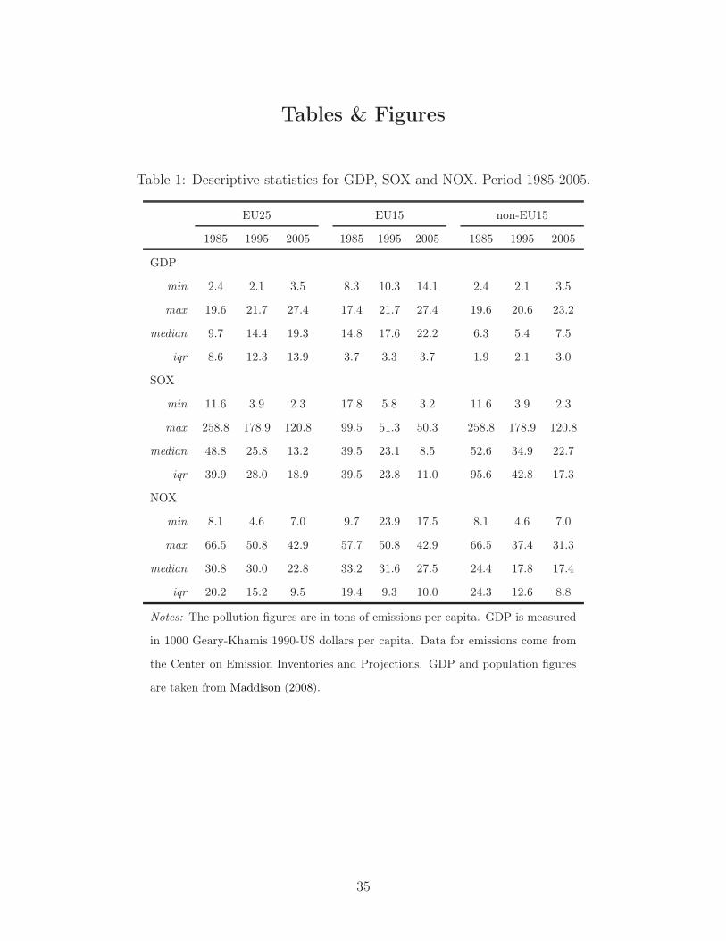
that all non-EU15 countries but Switzerland have substantially lower per capita GDP levels.

There is no clear evidence of a decreasing gap in per capita GDP either within or between

these two groups over the 1980-2005 period. This is confirmed by the descriptive statistics

reported in Table 1 where the difference in median income between the EU15 and the non-

EU15 countries strongly increases over time. By contrast, many of the downward sloping

NOX and SOX series in Figure 2 seem to stabilize at some point and converge in the sigma

sense across the whole sample. Both the global and the group-specific interquartile range

of emissions decrease over time in Table 1. Note however that the median level of NOX

emissions per capita remains typically higher in the EU15 while the reverse holds for SOX.

These patterns suggest the presence of two distinct groupings of countries that may display

different behaviors in the econometric analysis.

4.2 Regression results

Tables 2 and 3 contain the regression results for SOX and NOX respectively18. Columns (A)

to (D) test the presence of the scale and defensive effects in the parametric specifications with

a standard OLS fixed-effects estimator. These regressions also represent β-type convergence

equations for pollution, conditional upon the levels and growth rates of per capita GDP.

Columns (A) and (B) focus on specification (28) where column (B) is the IV counterpart of

(A), which controls for potential endogeneity bias. Columns (C) and (D) display the results

for the extended model (29) in the same manner. Column (E) shows the linear part of the

semiparametric regression with some diagnostic statistics. Column (F) displays the R2 of the

nonparametric estimates. Graphical devices (Figures 3 and 4 for SOX and NOX respectively)

complete the results by displaying linear, partially linear and fully nonparametric partial

relationships, for year t = 1985 and by EU15 status, keeping all other continuous factors at

were dropped.18All the econometric results and figures presented in this paper are obtained with the software R.2.12.1.

23

their respective medians.

Looking at the results for SOX emissions, Table 2 shows that none of the parametric

regressions display heteroscedasticity, as the null of homoscedasticity cannot be rejected with

the Breusch-Pagan test at conventional significance levels19. Therefore, the usual coefficients’

standard deviation can be safely used to assess significance. The SOX dynamics appear to

be globally unaffected by time-shocks over the period under scrutiny except for the year

1995. The defensive effect in the linear models (A) and (B) is not always significant, while

the expected scale effect exists and is highly significant in both the short and the extended

parametric specifications. Taking into account the GDP variable in models (C) and (D)

improves the explanatory power of the parsimonious specifications (A) and (B), i.e., the

adjusted R2 increases substantially. However, applying the specification test20 to the OLS

fits (last line in Table 2), all parametric models are rejected at the 5% level. Therefore a closer

look at the flexible estimates is necessary and we expect them to depict nonlinearities as well

as potentially different patterns, specific to the EU15 membership for the fully nonparametric

regressions21. The PLR estimates in column (E) confirm that a structural shock affected the

pollution dynamics in 1995, and that the greater flexibility introduced in the continuous

regressors clearly increases the explanatory power of model (D). We also observe that the

misspecification test does not reject the PLR regression (E), and that the fully nonparametric

model (F) captures 12% of additional total variance with respect to its semiparametric

counterpart. We now proceed to evaluate the fits obtained with the flexible models with

partial regression plots22. Note that the linear estimates are also shown for comparison19We used the routine bptest from package lmtest-0.9-27 to perform the Breusch-Pagan LM test and the

function hccm from package car-2.0-9 to compute White-corrected covariance matrices when heteroscedas-ticity was detected (see NOX regressions).

20We used the routine npcmstest from package n.p-0.40-4 to apply Hsiao et al. (2007)’s misspecificationtest.

21The PLR estimates have been computed with the gam function from package mgcv-1.7-2.22The bandwidths of the nonparametric regressions presented in this paper are available in the supplemen-

tary material at the online archive. They are all computed with function npregbw from package np-0.40-4.The partial regression plots have been partly generated with the help of package plotrix-3.0-9.

24

purposes.

The upper graphs in Figure 3 show that the defensive effect linked to initial pollution

levels is confirmed for the EU15 as well as for the non-EU15 countries with both the PLR and

the fully nonparametric models. The least-square cross-validation methodology employed to

determine the bandwidths does not detect departures from linearity for that partial relation-

ship. The scale effect linked to GDP growth is shown in the middle plots: it is positive as

expected, with larger partial elasticities for GDP growth in the EU15 countries. However, the

scale effect for the non-EU15 group is hump-shaped with the fully nonparametric fit23. The

initial GDP variable introduced to capture potential nonlinearities appear to have a negative

but linear impact on pollution growth. Overall, despite the rejection of the parametric spec-

ifications by the data, the flexible estimates indicate that SOX emissions in Europe display

a dynamic income-pollution relation that is consistent with our model’s prediction.

The results for NOX depart from the SOX ones in several important aspects. First, as

shown in Table 3, the explanatory power of the models is typically larger and all parametric

regressions display heteroscedastic errors. Therefore, the coefficients’ standard deviation for

the parametric fits are White-corrected while those of the linear part of the semiparametric

model rely on a Bayesian approach (Wood, 2006). We observe that the coefficients are

significant across all models. Taking into account the GDP variable in models (C) and (D)

does not significantly improve the explanatory power of the parsimonious specifications (A)

and (B) as the R2s remain very similar. Second, regressions (A) and (B) clearly establish the

existence of both the defensive and scale effects, as well as β-convergence for NOX emissions

across Europe, with significantly larger growth rates within the EU15 countries. Adding

the GDP levels in specifications (C) and (D) does not change these results. Third, the

misspecification tests conclude that most linear models are misspecified at the significance

level of 10%. The short linearized equation (28) seems to match the data better than23The partial relationships for SOX for alternative levels of the time factor t = {1990, 1995, 2000} remain

robust, see the supplementary material at the online archive.

25

the expanded linear models (C) and (D): both (A) and (B) regressions would pass the

specification test if we required stronger evidence of misspecification, say 5% or 1% cutoffs, to

reject the null of correct specification. In order to check whether the rejection of the extended

specification is due to a lack of flexibility in the parametric specification, we estimate the IV

model (D) within a PLR structure. Column (E) shows that the PLR model is not rejected

and confirms that significant time-shocks have affected the NOX dynamics over the observed

period.

Fourth, given the uncertainty regarding the most appropriate specification for NOX –

model (B) versus model (E) – we proceed in column (F) with a fully flexible approach,

i.e., the IV model (D) estimated with a fully nonparametric regression. Before moving to

the partial regression plots, note that the latter model explains 88% of the total variance

(see column (F) in Table 3). The upper plots in Figure 4 corroborate the existence of

a defensive effect for both country groupings with the PLR as well as the nonparametric

models. The middle plots confirm the positive effect of GDP growth on pollution growth

(again, with larger partial elasticities in the EU15 economies). The effect of the initial GDP

on the subsequent pollution growth rates is nonlinear but ambiguous, as the confidence

interval includes the zero over large portions of the support for both areas. Also, note that

the confidence interval surrounding the non-EU15 fits are globally larger. In sum, the path

followed since 1985 by the NOX emissions per capita is fully compatible with the convergence

equation predicted by the theoretical model, but with a stronger evidence holding within the

EU15 countries24.24The partial relationships for the fully nonparametric regressions are potentially different for alternative

levels of the time factor t = {1990, 1995, 2000}. The scale effect remains clearly positive over time for NOXwhile the defensive effect tends to become flatter. These results are available in the supplementary materialat the online archive.

26

5 Conclusion

Growth theories are particularly useful to unveil transitional or long-run relationships be-

tween pollution, capital accumulation and other central determinants of economic growth

(Xepapadeas, 2005). In this paper, we develop a growth model of a representative economy

where the interplay between purposeful abatement of pollution, technological progress and

diminishing return of capital generates an optimal growth path characterized by a precise

dynamic law: the growth rate of emissions per capita is (i) negatively related to the level

of emissions per capita and (ii) positively related to the growth rate of output per capita.

Result (i) is a ‘defensive effect’ reflecting the effectiveness of abatement expenditures in lim-

iting pollution growth. Result (ii) is a ‘scale effect’ implied by the positive relation between

output and emission levels. This dynamic law can be interpreted as a β-convergence equa-

tion: by virtue of the defensive effect, pollution growth rates regress to zero and emissions

per capita are bounded in the long run.

This theoretical prediction is tested for a panel of 25 European countries on per capita

SOX and NOX emissions spanning the years 1980 to 2005. Regression estimates based

on linear models as well as semi-parametric and fully nonparametric methods support the

model predictions, identifying a clear scale effect linked to GDP growth and a negative effect

captured through the impact of the past pollution level component.

Acknowledgments

Preliminary results for this paper were presented at the Fourth World Congress of Environ-

mental and Resource Economists 2010 in Montreal (Canada), at SURED 2010 in Ascona

(Switzerland) and at the 64th Econometric Society European meeting 2009 in Barcelona

(Spain). We are grateful to Arik Levinson, Charles F. Mason and two anonymous Referees

for insightful comments that significantly improved the paper. The usual disclaimer applies.

27

Appendix

Derivation of (10)-(11) Substituting c = cB and p = pB in the utility function (6), the

current-value Hamiltonian associated with the optimal control problem is

H (c, p, χ, k) = σ ln (cB)− ς (pB)θ + λk [f (k) (1− χ)− c− (δ + n + π) k] +

+ λp [Ω (1− χ)ε f (k)− p] ,

where λk is the dynamic multiplier for constraint (8) and λp is the Lagrange multiplier for

constraint (9). The necessary conditions for optimality are

Hc = 0 λk = σc−1, (A-1)

Hp = 0 λp = −ςθpθ−1Bθ, (A-2)

Hχ = 0 λk = −λpΩε (1− χ)ε−1 , (A-3)

together with the co-state equation

Hk = ρλk − λk → λk/λk = ρ+ δ + n + π − fk (1− χ)(1− ε−1

), (A-4)

where we have used λk/λp = −Ωε (1− χ)ε−1 from (A-3). Time-differentiation of (A-1) yields

c/c = −λk/λk, which can be plugged into (A-4) to obtain (10). Combining (A-1), (A-2) and

(A-3) to eliminate λk and λp, we obtain

Ωε (1− χ)ε−1 ςθpθ−1Bθ = σc−1,

where we can substitute p = Ω(1− χ)ε f (k) from (9) to obtain

(1− χ)εθ−1 =

[σ

εςθ (ΩB)θ

]f (k)1−θ

c. (A-5)

28

Because Ω (t)B (t) = Ω0B0 is constant, the term in square brackets in (A-5) is constant.

Solving (A-5) for (1− χ), and defining Γ ≡[εςθ (Ω0B0)

θ σ−1]−1/(εθ−1)

, we obtain (11).

Proof of Lemma 1 The existence, uniqueness and saddle-point stability of the steady

state (css, kss) are proved in detail in the Appendix available at the online archive. Note that

saddle-point stability of (css, kss) is directly connected to saddle-point stability of (pss, kss);

the latter result is proved below for the Cobb-Douglas case.

Derivation of system (19)-(20) From (17), we have

c = (Ω0B0Γε)

εθ−1ε p−

εθ−1ε f (k)1−

1ε . (A-6)

Plugging (A-6) in (13), the growth rate of k (t) equals

g (k) = (f (k) /k) Φ (k, c)− (Ω0B0Γε)

εθ−1ε p−

εθ−1ε (f (k) /k) f (k)−

1ε − (ρ− ρ) ,

where we can substitute Φ (k, c) = (Ω0B0)− 1

ε p1ε f (k)−

1ε from (17) to obtain

g (k) = (f (k) /k) f (k)−1ε (Ω0B0)

− 1ε p

1ε

[1− (

Ωθ0B

θ0Γ

εθ−1)p (t)−θ

]− (ρ− ρ) . (A-7)

When the technology is Cobb-Douglas, f (k) = kα, we have (f (k) /k) f (k)−1ε = kα−1−α/ε.

Plugging this result in (A-7), and defining the constants ϕ2 ≡ (Ω0B0)− 1

ε > 0, ϕ3 ≡Ωθ

0Bθ0Γ

εθ−1 = σ/ (ςεθ) > 0 and ϕ4 ≡ ρ− ρ = δ + n+ π > 0, we obtain (20). As regards (19),

re-write (14) as

g (c) = α (f (k) /k) Φ (k, c)

(ε− 1

ε

)− ρ, (A-8)

29

where we have used fk = α (f (k) /k) and g (c) ≡ c/c for the consumption growth rate. Next

time-differentiate (17) to get

g (p) =ε− 1

εθ − 1g (f (k))− ε

εθ − 1g (c) , (A-9)

where, given f (k) = kα, the growth rate of normalized output equals g (f (k)) = αg (k).

Plugging g (f (k)) = αg (k) and substituting g (k) with (A-7), and substituting g (c) by

means of (A-8), we obtain

g (p) =ερ− α (ρ− ρ) (ε− 1)

εθ − 1− ε− 1

εθ − 1α (f (k) /k) Φ (k, c)

(Ωθ

0Bθ0Γ

εθ−1)p−θ. (A-10)

Substituting Φ (k, c) = (Ω0B0)− 1

ε p1ε f (k)−

1ε from (17), and defining the constants ϕ0 ≡

ερ−α(ρ−ρ)(ε−1)εθ−1

= ερ(1−α)+αρ+αρ(ε−1)εθ−1

> 0 and ϕ1 ≡ α ε−1εθ−1

(Ω0B0)θ− 1

ε Γεθ−1 > 0, we obtain (19).

Derivation of (23), (24) and (25) From (19), we have ∂g (p) /∂p > 0 and ∂g (p) /∂k > 0.

From (20), we have , ∂g (k) /∂p > 0 and ∂g (k) /∂k < 0. Hence, the coefficient matrix

of the linearized system is given by m1 ≡ ∂g (p) /∂p|pss > 0, m2 ≡ ∂g (p) /∂k|pss > 0,

m3 ≡ ∂g (k) /∂p|kss > 0, m4 ≡ ∂g (k) /∂k|kss < 0. Given these signs, system (23)-(24)

displays two real roots of opposite signs, the stable root being

μ ≡ (1/2)

[(m1 +m4)−

√(m1 +m4)

2 − 4 (m1m4 −m2m3)

]< 0.

The stable arm equation is given by k(t)−kssp(t)−pss

= μ−m1

m2, where μ < 0, m1 > 0, and m2 > 0

imply that the right hand side is a strictly negative constant, φ ≡ μ−m1

m2< 0.

Derivation of (26) and proof of Proposition 2 Since output per capita equals y (t) =

B (t) k (t)α, its growth rate is given by g (y (t)) = π + αg (k (t)). Plugging (24) in this

expression, we have

30

g (y (t)) = π + α [m3 (p (t)− pss) +m4 (k (t)− kss)] .

Eliminating (k (t)− kss) by means of the stable-arm equation (25) and rearranging terms

yields

(p (t)− pss) =g (y (t))− π

α (m3 +m4φ).

Plugging this expression in (23), and using (25) to eliminate (k (t)− kss), we obtain (26).

Defining H1 ≡ m1

α(m3+m4φ), H2 ≡ −φm2 and H0 ≡ H2pss − πH1, we obtain equation (26) in

Proposition 2. Since α > 0, m1 > 0, m2 > 0, m3 > 0, m4 < 0 and φ < 0, coefficients H1 and

H2 are both strictly positive, which completes the proof. �

References

Acemoglu, D. (2009) Introduction to Modern Economic Growth (Princeton NJ: Princeton

University Press)

Aldy, J.E. (2006) ‘Per capita carbon dioxide emissions: Convergence or divergence.’ Envi-

ronmental and Resource Economics 33(4), 533–555

Barro, R.J., and X. Sala-i-Martin (2004) Economic Growth, second ed. (Massachusetts: The

MIT Press)

Bovenberg, A.L., and J. Smulders (1995) ‘Environmental quality and pollution-augmenting

technological change in a two-sector endogenous growth model.’ Journal of Public Eco-

nomics 57(3), 353–360

Bratberg, E., S. Tjotta, and T. Oines (2005) ‘Do voluntary environmental agreements work?’

Journal of Environmental Economics and Managment 50(3), 583–597

31

Breusch, T.S., and A.R. Pagan (1979) ‘A simple test for heteroscedasticity and random

coefficient variation.’ Econometrica 47(5), 1287–1294

Brock, W.A., and M.S. Taylor (2005) ‘Economic growth and the environment: a review of

theory and empirics.’ In Handbook of Economic Growth, ed. Philippe Aghion and Steven N.

Durlauf (Elsevier) pp. 1750–1821. Volume 1B

(2010) ‘The green solow model.’ Journal of Economic Growth 15(2), 127–153

Bulte, E., J. List, and M.C. Strazicich (2007) ‘Regulatory federalism and the distribution of

air pollutant emissions.’ Journal of Regional Science 47(1), 155–178

Evans, P., and G. Karras (1996) ‘Do economies converge? evidence from a panel of u.s.

states.’ The Review if Economics and Statistics 78(3), 384–388

Finus, M., and S. Tjotta (2003) ‘The oslo protocol on sulfur reduction: the great leap

forward?’ Journal of Public Economics 87(9-10), 2031–2048

Friedman, M. (1992) ‘Do old fallacies ever die.’ Journal of Economic Literature 30(4), 2129–

2132

Greene, W.H. (2008) Econometric Analysis, sixth ed. (Prentice Hall International)

Hsiao, C., Q. Li, and J.S. Racine (2007) ‘A consistent model specification test with mixed

categorical and continuous data.’ Journal of Econometrics 140(2), 802–826

Keeler, E., M. Spence, and R. Zeckhauser (1971) ‘The optimal control of pollution.’ Journal

of Economic Theory 4(1), 19–34

Koenker, R. (1981) ‘A note on studentizing a test for heteroscedasticity.’ Journal of Econo-

metrics 17(1), 107–112

Li, Q., and J.S. Racine (2007) Nonparametric Econometrics (New Jersey: Princeton Univer-

sity Press)

32

List, J.A. (1999) ‘Have air pollutant emissions converged among u.s. regions? evidence from

unit root tests.’ Southern Economic Journal 66(1), 144–155

Maasoumi, E., J. Racine, and T. Stengos (2007) ‘Growth and convergence: A profile of

distribution dynamics and mobility.’ Journal of Econometrics 136(2), 483–508

Maddison, A. (2008) ‘Historical statistics.’ Online data, Groningen Growth and Development

Center, University of Groningen„ October. http://www.ggdc.net/maddison

Mankiw, N Gregory, David Romer, and David N Weil (1992) ‘A contribution to the empirics

of economic growth.’ The Quarterly Journal of Economics 107(2), 407–37

Mareckova, K, R. Wankmueller, M. Anderl, B. Muik, S. Poupa, and M. Wieser (2008)

‘Inventory review 2008.’ Technical Report, European Environment Agency and Centre on

Emission Inventories and Projections

Murdoch, J.C., T. Sandler, and K. Sargent (1997) ‘A tale of two collectives: Sulphur versus

nitrogen oxides emission reduction in europe.’ Economica 64(254), 281–301

Nguyen Van, P. (2005) ‘Distribution dynamics of co2 emissions.’ Environmental and Resource

Economics

Ordás Criado, C., and J.-M. Grether (forthcoming) ‘Convergence in co2 per capita emissions:

a robust distributional approach.’ Resource and Energy Economics

Quah, D. (1993a) ‘Empirical cross-sectional dynamics in economic growth.’ European Eco-

nomic Review 37(2-3), 426–434

(1993b) ‘Galton’s fallacy and tests of the convergence hypothesis.’ Scandinavian Journal

of Economics 95(4), 427–443

Racine, J., and Q. Li (2004) ‘Nonparametric estimation of regression functions with both

categorical and continuous data.’ Journal of Econometrics 119(1), 99–130

33

Romero-Ávila, D. (2008) ‘Convergence in carbon dioxide emissions among industrialised

countries revisited.’ Energy Economics 30(5), 2265–2282

Shioji, E. (1997) ‘It’s still 2%: Evidence on convergence from 116 years of the us states panel

data.’ Working paper 236, Universitat Pompeu Fabra

Strazicich, M.C., and J.A. List (2003) ‘Are co2 emissions levels converging among industrial

countries?’ Environmental and Resource Economics 24(3), 263–271

UN Economic Commission for Europe (2009) ‘Guidelines for reporting emission data

under the convention on long-range transboundary air pollution.’ Technical Report:

ECE/EB.AIR/97, United Nations - Economic Commission for Europe

Van der Ploeg, F., and C. Withagen (1991) ‘Pollution control and the ramsey problem.’

Environmental and Resource Economics 1(2), 215–236

Wood, S. (2006) Generalized Additive Models: An Introduction with R (Chapman & Hall,

Texts in Statistical Sciences)

Xepapadeas, A. (2005) ‘Economic growth and the environment.’ In Handbook of Environmen-

tal Economics, ed. K.-G. Maler and J.R. Vincent (Elsevier B.V.) pp. 1219–1271. Volume

3

34

Tables & Figures

Table 1: Descriptive statistics for GDP, SOX and NOX. Period 1985-2005.

EU25 EU15 non-EU15

1985 1995 2005 1985 1995 2005 1985 1995 2005

GDP

min 2.4 2.1 3.5 8.3 10.3 14.1 2.4 2.1 3.5

max 19.6 21.7 27.4 17.4 21.7 27.4 19.6 20.6 23.2

median 9.7 14.4 19.3 14.8 17.6 22.2 6.3 5.4 7.5

iqr 8.6 12.3 13.9 3.7 3.3 3.7 1.9 2.1 3.0

SOX

min 11.6 3.9 2.3 17.8 5.8 3.2 11.6 3.9 2.3

max 258.8 178.9 120.8 99.5 51.3 50.3 258.8 178.9 120.8

median 48.8 25.8 13.2 39.5 23.1 8.5 52.6 34.9 22.7

iqr 39.9 28.0 18.9 39.5 23.8 11.0 95.6 42.8 17.3

NOX

min 8.1 4.6 7.0 9.7 23.9 17.5 8.1 4.6 7.0

max 66.5 50.8 42.9 57.7 50.8 42.9 66.5 37.4 31.3

median 30.8 30.0 22.8 33.2 31.6 27.5 24.4 17.8 17.4

iqr 20.2 15.2 9.5 19.4 9.3 10.0 24.3 12.6 8.8

Notes: The pollution figures are in tons of emissions per capita. GDP is measured

in 1000 Geary-Khamis 1990-US dollars per capita. Data for emissions come from

the Center on Emission Inventories and Projections. GDP and population figures

are taken from Maddison (2008).

35

Table 2: Regressions results. SOX pollution growth vs. initial pollution levels and GDP.

Parametric models Non/semipa. models

Ordinary LS PLR fit(a) NP fit(b)

Variables (A) (B) (C) (D) (E) (F)

constant 0.013 0.007 0.153*** 0.145*** -0.078*** -

d1990 -0.023 -0.020 -0.025 -0.022 -0.020 -

d1995 -0.041** -0.040** -0.041** -0.041** -0.042** -

d2000 -0.026 -0.024 -0.020 -0.020 -0.027 -

EU15 -0.032** -0.030** 0.029 0.029 0.066** -

Pi,t−T (β) -0.013* -0.011 -0.021*** -0.019** - -

GYi,t (γ1) 0.802*** - 0.653** - - -

GYi,t−1 (γ1,IV ) - 0.719*** - 0.563** - -

Yi,t−T (γ2) - - -0.063*** - - -

Yi,(t−1)−T (γ2,IV ) - - - -0.062*** - -

N 100 100 100 100 100 100

R2/R2 adj. 0.17/0.11 0.16/0.11 0.28/0.22 0.27/0.22 0.48/0.40 0.60/-

F-stat 3.12*** 3.06*** 5.02*** 4.94*** - -

Heterosced. LM-stat.(a) 5.08 4.40 8.71 8.12 - -

P(Correct. Specific.)(b) 0.020 0.010 0.002 0.005 0.193 -

Notes: ***, ** and * denote the 1%, 5% and 10% significance levels. (a) : ‘Heterosced. LM-stat.’

is the heteroscedasticity LM-statistic of Breusch and Pagan (1979), computed with the variance

estimator robust to departure from normality proposed by Koenker (1981). Under the null of ho-

moscedasticity, the statistic is χ2-distributed, with d.f. = nb. of regressors (constant excluded).

(b): ‘P(Correct. Specific.)’ stands for the probability associated to the nonparametric specifica-

tion test by Hsiao et al. (2007) for continuous and discrete data models under the null of correct

specification. The latter probability is based on 399 iid bootstrap’s replications.

36

Table 3: Regression results. NOX pollution growth vs. initial pollution levels and GDP.

Parametric models Non/semipa. models

Ordinary LS PLR fit NP fit

Variables (A) (B) (C) (D) (E) (F)

constant 0.125*** 0.120*** 0.130*** 0.126*** -0.028*** -

d1990 -0.026*** -0.025*** -0.026*** -0.024*** -0.021*** -

d1995 -0.039*** -0.039*** -0.037*** -0.038*** -0.034*** -

d2000 -0.039*** -0.039*** -0.035*** -0.035*** -0.035*** -

EU15 0.019** 0.018** 0.028* 0.029*** 0.062*** -

Pi,t−T (β) -0.041*** -0.039*** -0.036*** -0.033*** - -

GYi,t (γ1) 0.667*** - 0.642*** - - -

GYi,t−1 (γ1,IV ) - 0.613*** - 0.588*** - -

Yi,t−T (γ2) - - -0.010* - - -

Yi,(t−1)−T (γ2,IV ) - - - -0.015** - -

N 100 100 100 100 100 100

R2/R2 adj. 0.54/0.51 0.54/0.51 0.55/0.52 0.55/0.52 0.71/0.66 0.88/-

F-stat. 18.3*** 18.2*** 16.7*** 16.4*** - -

Heterosced. LM-stat.(a) 16.4** 17.1*** 17.6** 18.8*** - -

P(Correct. Specific.)(b) 0.073 0.155 0.000 0.003 0.882 -

Notes: ***, ** and * denote the 1%, 5% and 10% significance levels. (a) : ‘Heterosced. LM-stat.’

is the heteroscedasticity LM-statistic of Breusch and Pagan (1979), computed with the variance

estimator robust to departure from normality proposed by Koenker (1981). Under the null of ho-

moscedasticity, the statistic is χ2-distributed, with d.f. = nb. of regressors (constant excluded).

(b): ‘P(Correct. Specific.)’ stands for the probability associated to the nonparametric specifica-

tion test by Hsiao et al. (2007) for continuous and discrete data models under the null of correct

specification. The latter probability is based on 399 iid bootstrap’s replications.

37

Figure 1: Phase diagram of capital vs pollution.

Notes: Phase diagram of system (19)-(20): saddle-point

stability of the joint dynamics of capital per efficient la-

bor, k (t), and pollution per capita, p (t). The optimal

trajectory of capital per efficient labor and pollution per

capita with initial condition k (0) = k0 < kss is given by

the arrowed line.

38

Fig

ure

2:Per

capi

tale

vels

ofG

DP,

SOX

and

NO

X.E

urop

ean

coun

trie

s,na

tion

altr

ends

1980

-200

5.

1980

1985

1990

1995

2000

2005

0510152025

GD

P

Year

s

1000 Geary−Khamis 1990−USD per capita

AL

ATBE

BG

CZ

S

DK FI

FR

DE

GR

HUIE ITNL

NO

PL

PT

RO

ES

SE

CH

TR

GB

YU

US

SR

EU

15N

on−

EU

15

1980

1985

1990

1995

2000

2005

050100150200250

SO

X

Year

s

Tons per capita

AL

AT BE

BG

CZ

S

DKFI

FR

DE

GR

HU IE IT NL

NO

PL

PT

RO

ES

SE

CH

TR

GB

YU

US

SR

EU

15N

on−

EU

15

1980

1985

1990

1995

2000

2005

0204060

NO

X

Year

s

Tons per capita

AL

AT BE

BG

CZ

S

DKFI

FR

DE

GR

HU IEITNL

NO

PL

PT

RO

ES

SE

CH

TR

GB

YU

US

SR

EU

15N

on−

EU

15

Not

es:

Yea

rly

GD

Pan

dpo

pula

tion

figur

esco

me

from

Mad

diso

n(2

008)

.E

mis

sion

sda

taar

eta

ken

from

the

Cen

ter

onE

mis

sion

Inve

ntor

ies

and

Pro

ject

ions

and

are

avai

labl

efo

rth

esp

ecifi

cye

ars

1980

,198

5an

d19

90an

don

aye

arly

basi

sla

ter

on.

39

Figure 3: Nonparametric partial regressions by EU15 status : SOX pollution growth vs.initial pollution levels and GDP.

Pol

lutio

n gr

owth

EU15 − Pollution growth vs Initial Pollution

Initial Pollution

2.1 2.5 2.9 3.3 3.7 4.1 4.5 4.9

−0.20

−0.16

−0.12

−0.08

−0.04

0.00

0.04

0.08 nonparam. fit +/− 95% c.i.OLS fitPLR fit

Pol

lutio

n gr

owth

non−EU15 − Pollution growth vs Initial Pollution

Initial Pollution

2.1 2.5 2.9 3.3 3.7 4.1 4.5 4.9

−0.20

−0.16

−0.12

−0.08

−0.04

0.00

0.04

0.08 nonparam. fit +/− 95% c.i.OLS fitPLR fit

Pol

lutio

n gr

owth

EU15 − Pollution growth vs GDP growth

GDP growth

−0.20

−0.16

−0.12

−0.08

−0.04

0.00

0.04

0.08 nonparam. fit +/− 95% c.i.OLS fitPLR fit

Pol

lutio

n gr

owth

non−EU15 − Pollution growth vs GDP growth

GDP growth

−0.20

−0.16

−0.12

−0.08

−0.04

0.00

0.04

0.08 nonparam. fit +/− 95% c.i.OLS fitPLR fit

Pol

lutio

n gr

owth

EU15 − Pollution growth vs Initial GDP

Initial GDP

2.1 2.5 2.9

−0.20

−0.16

−0.12

−0.08

−0.04

0.00

0.04

0.08

Pol

lutio

n gr

owth

non−EU15 − Pollution growth vs Initial GDP

Initial GDP

2.1 2.5 2.9

−0.20

−0.16

−0.12

−0.08

−0.04

0.00

0.04

0.08 nonparam. fit +/− 95% c.i.OLS fitPLR fit

Notes: Nonparametric regressions based on Racine and Li (2004).

40

Figure 4: Nonparametric partial regressions by EU15 status : NOX pollution growth vs.initial pollution levels and GDP.

Pol

lutio

n gr

owth

EU15 − Pollution growth vs Initial Pollution

Initial Pollution

3.0 3.3 3.6 3.9 4.2

−0.20

−0.16

−0.12

−0.08

−0.04

0.00

0.04

0.08 nonparam. fit +/− 95% c.i.OLS fitPLR fit

Pol

lutio

n gr

owth

non−EU15 − Pollution growth vs Initial Pollution

Initial Pollution

2.0 2.4 2.8 3.2 3.6 4.0

−0.20

−0.16

−0.12

−0.08

−0.04

0.00

0.04

0.08 nonparam. fit +/− 95% c.i.OLS fitPLR fit

Pol

lutio

n gr

owth

EU15 − Pollution growth vs GDP growth

GDP growth

−0.20

−0.16

−0.12

−0.08

−0.04

0.00

0.04

0.08 nonparam. fit +/− 95% c.i.OLS fitPLR fit

Pol

lutio

n gr

owth

non−EU15 − Pollution growth vs GDP growth

GDP growth

−0.20

−0.16

−0.12

−0.08

−0.04

0.00

0.04

0.08 nonparam. fit +/− 95% c.i.OLS fitPLR fit

Pol

lutio

n gr

owth

EU15 − Pollution growth vs Initial GDP

Initial GDP

2.0 2.3 2.6 2.9

−0.20

−0.16

−0.12

−0.08

−0.04

0.00

0.04

0.08 nonparam. fit +/− 95% c.i.OLS fitPLR fit

Pol

lutio

n gr

owth

non−EU15 − Pollution growth vs Initial GDP

Initial GDP

1.2 1.6 2.0 2.4 2.8

−0.20

−0.16

−0.12

−0.08

−0.04

0.00

0.04

0.08 nonparam. fit +/− 95% c.i.OLS fitPLR fit

Notes: Nonparametric regressions based on Racine and Li (2004).

41