Group Theory

Robert Gilmore

Physics Department, Drexel University, Philadelphia, Pennsylvania 19104, USA

(Dated: October 3, 2012)

Printed from:Wiley-Mathematical/GroupChapter/group.tex on October 3, 2012

I. INTRODUCTION

Symmetry has sung its siren song to Physicists sincethe beginning of time, or at least since before there werePhysicists. Today the ideas of symmetry are incorpo-rated into a subject with the less imaginative and sug-gestive name of Group Theory. This Chapter introducesmany of the ideas of group theory that are important inthe natural sciences.

Natural philosophers in the past have come up withmany imaginative arguments for estimating physicalquantities. They have often used out-of-the-box methodsthat were proprietary to pull rabbits out of hats. Whenthese ideas were made available to a wider audience theywere often improved upon in unexpected and previouslyunimaginable ways. A number of these methods are pre-cursors of group theory. These are Dimensional Analysis,Scaling Theory, and Dynamical Similarity. We reviewthese three methods in Sec. II.

In Sec. III we get down to the business at hand, intro-ducing the definition of group and giving a small set ofimportant examples. These range from finite groups todiscrete groups to Lie groups. These also include trans-formation groups, which played an important if under-recognized roll in the development of classical physics, inparticular the theories of Special and General Relativity.The relation between these theories and group theory isindicated in Sec. IV.

Despite this important roll in the development ofPhysics, groups existed at the fringe of the Physics ofthe early 20th century. It was not until the theory ofthe linear matrix representations of groups was inventedthat the theory of groups migrated from the outer fringesto play a more central roll in Physics. Important pointsin the theory of representations are introduced in Sec.V. Representations were used in an increasingly imag-inative number of ways in Physics throughout the 20th

century. Early on they were used label states in Quantumsystems with a symmetry group: for example, the rota-tion group SO(3). Once states were named, degeneraciescould be predicted and computations simplified. Such ap-plications are indicated in Sec. VI. Later, they were usedwhen symmetry was not present, or just the remnant of abroken symmetry was present. When used in this sense,they are often called “dynamical groups.” This type ofuse grossly extended the importance of Group Theory

in Physics. As a latest tour de force in the develop-ment of Physics, they play a central roll in the creationof Gauge Theories, which describe the interactions be-tween Fermions and the Bosons that are responsible forthe interactions among the Fermions, and which lies atthe heart of the Standard Model. We provide the sim-plest example of a gauge theory, based on the simplestcompact one parameter Lie group U(1), in Sec. VIII.

For an encore, in Sec. IX we show how the theory ofthe special functions of mathematical physics (Legendreand associated Legendre functions, Laguerre and associ-ated Laguerre functions, Gegenbauer, Chebyshev, Her-mite, Bessel functions, and others) are subsumed underthe theory of representations of some low-dimensional Liegroups. The classical theory of special functions came tofruition in the mid 19th century, long before Lie groupsand their representations were even invented.

II. PRECURSORS TO GROUP THEORY

Barenblatt has given a beautiful derivation of Pythago-ras’ Theorem that is out-of-the-box and suggests some ofthe ideas behind Dimensional Analysis. The area of theright triangle ∆(a, b, c) is 1

2ab (Fig. 1). Dimensionally,the area is proportional to square of any of the sides, mul-tiplied by some factor. We make a unique choice of sideby choosing the hypotenuse, so that ∆(a, b, c) = c2×f(θ),θ is one of the two acute angles, and f(θ) 6= 0 unless θ = 0or π/2. Equating the two expressions

f(θ) =1

2

(ac

)(bc

)=

1

2

(b

c

)(ac

)symmetry

= f(π

2− θ)

(1)This shows (a) that the same function f(θ) applies forall similar triangles and (b) f(θ) = f(π2 − θ). The latterresult is due to reflection ‘symmetry’ of the triangle aboutthe bisector of the right angle: the triangle changes butits area does not. We need (a) alone to prove Pythagoras’Theorem. The proof is in the figure caption.

websearch: Pythagoras’ theorem Barenblatt

2

FIG. 1: The area of the large right triangle is the sumof the areas of the two similar smaller right triangles:∆(a, b, c) = ∆(d, f, a) + ∆(f, e, b), so that c2f(θ) =a2f(θ) + b2f(θ). Since f(θ) 6= 0 for a nondegenerateright triangle, a2 + b2 = c2.

A Dimensional Analysis

How big is a hydrogen atom?The size of the electron ‘orbit’ around the proton in

the hydrogen atom ought to depend on the electron massme, or more precisely the electron-proton reduced massµ = meMP /(me + MP ). It should also depend on thevalue of Planck’s constant h or reduced Planck’s constant~ = h/2π. Since the interaction between the proton andelectron is electromagnetic, of the form V (r) = −e2/r(Gaussian units), it should depend on e2.

Mass is measured in gm. The dimensions of the chargecoupling e2 are determined by recognizing that e2/r is a(potential) energy, with dimensions M1L2T−2. We willuse capital letters M , L, and T to characterize the threeindependent dimensional ‘directions’. As a result, thecharge coupling e2 has dimensions ML3T−2 and is mea-sured in gm(cm)3/sec2. The quantum of action ~ hasdimensions [~] = ML2T−1.

Constant Dimensions Value Units

µ M 9.10442× 10−28 gm~ ML2T−1 1.05443× 10−27 gm cm2 sec−1

e2 ML3T−2 2.30655× 10−19 gm cm3 sec−2

a0 L ? cmCan we construct something with the dimensions of

length from m, e2, and ~? To do this, we introduce threeunknown exponents a, b, and c and write

a0 ' ma (e2)b ~c = (M)a (ML3T−2)b (ML2T−1)c

= (M)a+b+c L0a+3b+2c T 0a−2b−c

(2)and set this result equal to the dimensions of whateverwe would like to compute, in this case the Bohr orbita0 (characteristic atomic length), with [a0] = L. Thisresults in a matrix equation 1 1 1

0 3 20 −2 −1

abc

=

010

(3)

We can invert this matrix to find 1 1 10 3 20 −2 −1

−1

=

1 −1 −10 −1 −20 2 3

(4)

This allows us to determine the values of the exponentswhich provide the appropriate combinations of impor-tant physical parameters to construct the characteristicatomic length: ab

c

=

1 −1 −10 −1 −20 2 3

010

=

−1−1

2

(5)

This result tells us that

a0 ∼ m−1(e2)−1(~)2 = ~2/me2 ∼ 10−8 cm (6)

To construct a characteristic atomic time, we can re-place the vector col[0, 1, 0] in Eq. (5) by the vectorcol[0, 0, 1], giving us the result τ0 ∼ ~3/m(e2)2. Fi-nally, to get a characteristic energy, we can form thecombination E ∼ML2T−2 = m(~2/me2)2(~3/me4)−2 =me4/~2. Another, and more systematic, way to get thisresult is to substitute the vector col[1, 2,−2] in Eq. (5).

Note that our estimate would be somewhat different ifwe had used h instead of ~ = h/2π in these arguments.We point out that this method is very useful for estimat-ing the order of magnitude of physical parameters andusually gets the prefactor within a factor of 10.

websearch: dimensional analysis

B Scaling

Positronium is a bound state of an electron e with apositron e, its antiparticle. How big is positronium?

To address this question we could work very hard andsolve the positronium Hamiltonian. Or we could be lazyand observe that the hydrogen atom radius is inverselyproportional to the reduced electron-proton mass, so thepositronium radius should be inversely proportional tothe reduced electron-positron mass: µpos. = meme/(me+me) = 1

2me since the electron and positron have equalmassesme = me. Since the reduced electron-proton massis effectively the electron mass, the positronium atom isapproximately twice as large as the hydrogen atom.

In a semiconductor it is possible to excite an electronfrom an almost filled (valence) band into an almost empty(conduction) band. This leaves a ‘hole’ behind in thevalence band. The positively charged hole in the valenceband interacts with the excited electron in the conductionband through a reduced Coulomb interaction: V (r) =−e2/εr. The strength of the interaction is reduced byscreening effects which are swept into a phenomenologicaldielectric constant ε. In addition, the effective massesm∗e of the excited electron and the left-behind hole m∗h

3

are modified from the free-space electron mass values bymany-particle effects.

How big is an exciton in Gallium Arsenide (GaAs)?For this semiconductor the phenomenological parametersare ε = 12.5, m∗e = 0.07me, m

∗h = 0.4me.

We extend the scaling argument above by comput-ing the reduced mass of the electron hole pair: µe−h =(0.07me)(0.4me)/(0.07 + 0.4)me = 0.06me and replacinge2 in the expression Eq. (4) for the Bohr radius a0 bye2/ε. The effect is to multiply a0 by 12.5/0.06 = 208.The ground state radius of the exciton formed in GaAsis about 10−6 cm. The ground state binding energy islower than the hydrogen atom binding energy of 13.6 eVby a factor of 0.06/12.52 = 3.8× 10−4 so it is 5.2 meV .

Scaling arguments such as these are closely related torenormalization group arguments as presented in Chap-ter XXX.

C Dynamical Similarity

Jupiter is about five times further (5.2AU) from ourSun than the Earth. How many earth years does it takefor Jupiter to orbit the Sun?

Landau and Lifshitz provide an elegant solution tothis simple question using similarity (scaling) arguments.The equation of motion for the Earth around the Sun is

mEd2xE

dt2E= −GmEMS

xE

|xE|2(7)

where xE is a vector from the sun to the earth and xE

the unit vector in this direction. If Jupiter is in a geo-metrically similar orbit, then xJ = αxE, with α = 5.2.Similarly, time will evolve along the Jupiter trajectoryin a scaled version of its evolution along the Earth’s tra-jectory: tJ = βtE . Substituting these scaled expressionsinto the equation of motion for Jupiter, and cancellingout mJ from both sides, we find

α

β2

d2xE

dt2E= − 1

α2GMS

xE

|xE|2(8)

This scaled equation for Jupiter’s orbit can only beequated to the equation for the Earth’s trajectory (the or-bits are similar) provided α3/β2 = 1. That is, β = α3/2,so that the time-scaling factor is 5.23/2 = 12.5.

We have derived Kepler’s Third Law without even solv-ing the equations of motion! Landau and Lifshitz pointout that you can do even better than that. You don’teven need to know the equations of motion to constructscaling relations when motion is described by a poten-tial V (x) which is homogeneous of degree k. This meansthat V (αx) = αkV (x). When the equations of motionare derivable from a Variational Principle δI = 0, where

TABLE I: Four important results in the historical devel-opment of science are consequences of scaling arguments.

k Scaling Law−1 T 2 ' D3 Kepler #3

0 D ' T Newton #1+1 ∆z ' ∆t2 Galileo : Rolling Stones+2 T ' D0 Hooke

I =

∫ (m

(dx

dt

)2

− V (x)

)dt (9)

then the scaling relations x→ x′ = αx, t→ t′ = βt leadto a modified action

I ′ =α2

β

∫ (m

(dx

dt

)2

− αk−2β2V (x)

)dt (10)

The Action I ′ is proportional to the original Action I,and therefore leads to the same equations of motion,only when αk−2β2 = 1. That is, the time elapsed, T ,is proportional to the distance traveled, D, according toT ' D(1−k/2). Four cases are of interest.

k=−1 (Coulomb/Gravitational Potential) The periodof a planetary orbit scales like the 3/2 power of the dis-tance from the Sun (Kepler’s Third Law).

k= 0 (No forces) The distance traveled is proportionalto the time elapsed (essentially Newton’s First Law). Torecover Newton’s first law completely it is only necessaryto carry out the variation in Eq. (10), which leads toddt

(dxdt

)= 0.

k=+1 (Free fall in a homogeneous gravitational field)The potential V (z) = mgz describes free fall in a ho-mogeneous graviational field. Galileo is reputed to havedropped rocks off the Leaning Tower of Pisa to determinethat the distance fallen was proportional to the square ofthe time elapsed. The story is apocryphal: in fact, herolled stones down an inclined plane to arrive at the re-sult ∆z ' ∆t2.

k=+2 (Harmonic oscillator potential) The period isindependent of displacement: β = 1 independent of α.Hooke’s law, F = −kx, V (x) = 1

2kx2 leads to oscillatory

motion whose frequency is independent of the amplitudeof motion. This was particularly useful for constructingrobust clocks.

These four historical results in the development of earlyscience are summarized in Table I and Fig. 2.

websearch: dynamical similarity

4

FIG. 2: Four substantial advances in the developmentof early Physics are summarized. Each is a consequenceof using a homogeneous potential with a different degreek in a variational description of the dynamics. Scalingrelates the size scale of the trajectory α to the time scaleβ = αp, p = 1− 1

2k of the motion.

III. GROUPS

In this Section we finally get to the point of definingwhat a group is by stating the group axioms. These areillustrated with a number of examples: the two-elementgroup, the group of the equilateral triangle, finite groups,the permutation group, discrete groups, point groups andspace groups. Then we introduce groups of transforma-tions in space as matrix groups. Lie groups are intro-duced and examples of matrix Lie groups are presented.Lie groups are linearized to form their Lie algebras, andgroups are recovered from their algebras by reversing thelinearization procedure using the exponential mapping.Many of the important properties of Lie algebras are in-troduced, including isomorphisms among different rep-resentations of a Lie algebra. A powerful disentanglingtheorem is presented and illustrated in a very simple casethat plays a prominent role in the field of Quantum Op-tics. We will use this result in the Section on SpecialFunctions.

A Group Axioms

A group G consists of — a set of group elementsg1, g2, g3, · · · ∈ G together with an operation , calledgroup multiplication — that satisfy the following fouraxions:

Closure: gi ∈ G, gj ∈ G⇒ gi gj ∈ G

Associativity: (gi gj) gk = gi (gj gk)

Identity: g1 gi = gi = gi g1

Unique Inverse: gk gl = g1 = gl gk

Group multiplication has two inputs and one output.The two inputs must be members of the set. The firstaxiom (Closure) requires that the output must also bea member of the set.

The composition rule does not allow us to multiplythree input arguments. Rather, two can be combined toone, and that output can be combined with the third.This can be done in two different ways that preservesthe order (i, j, k). The second axiom (Associativity)requires that these two different ways give the same finaloutput.

The third axiom (Identity) requires that a specialgroup operation exists. This, combined with any opera-tion, gives back exactly that operation.

The fourth axiom (Unique Inverse) guarantees thatfor each group element, there is another uniquely definedgroup element, with the property that the product of thetwo is the unique identity element.

Remark 1 — Indexes: The notation (subscriptsi, j, k, · · · ) may suggest that the indices are inte-gers. This is not generally true: for continuousgroups the indices are points in some subspace ofa Euclidean space or more complicated manifold.

Remark 2 — Commutativity: In general the outputof the group multiplication depends on the orderof the inputs: gi gj 6= gj gi. If the result isindependent of the order the group is said to becommutative.

websearch: group theory physicsThe group operations in some previous examples

(Pythagoras, Scaling, Dynamical Similarity) involve mul-tiplication by one or more real numbers (continuousgroups). For the dimensional analysis example it wasmultiplication by integer powers of fundamental physicalconstants (discrete group).

It is not entirely obvious that the Unique Inverse ax-iom is needed. It is included among the axioms becausemany of our uses involve relating measurements made bytwo observers. For example, if Allyson on the Earth canpredict something about the length of a year on Jupiter,then Bob on Jupiter should just as well be able to pre-dict the length of Allyson’s year on Earth. Basically,this axiom is an implementation of Galileo’s Principle ofRelativity.

B Finite Groups

1 The Two-Element Group Z2

The simplest nontrivial group has one additional oper-ation beyond the identity e: G = e, f with f f = e.This group can act in our three-dimensional space R3 inseveral different ways:

5

Reflection: (x, y, z)f=σZ→ (+x,+y,−z)

Rotation: (x, y, z)f=RZ(π)→ (−x,−y,+z)

Inversion: (x, y, z)f=P→ (−x,−y,−z)

These three different actions of the order-two group onR3 describe: reflections in the x-y plane, σZ ; rotationsaround the Z axis through π radians, RZ(π); and inver-sion in the origin, the parity operation, P. They can bedistinguished by their matrix representations, which are

σZ RZ(π) P +1 0 00 +1 00 0 −1

−1 0 00 −1 00 0 +1

−1 0 00 −1 00 0 −1

(11)

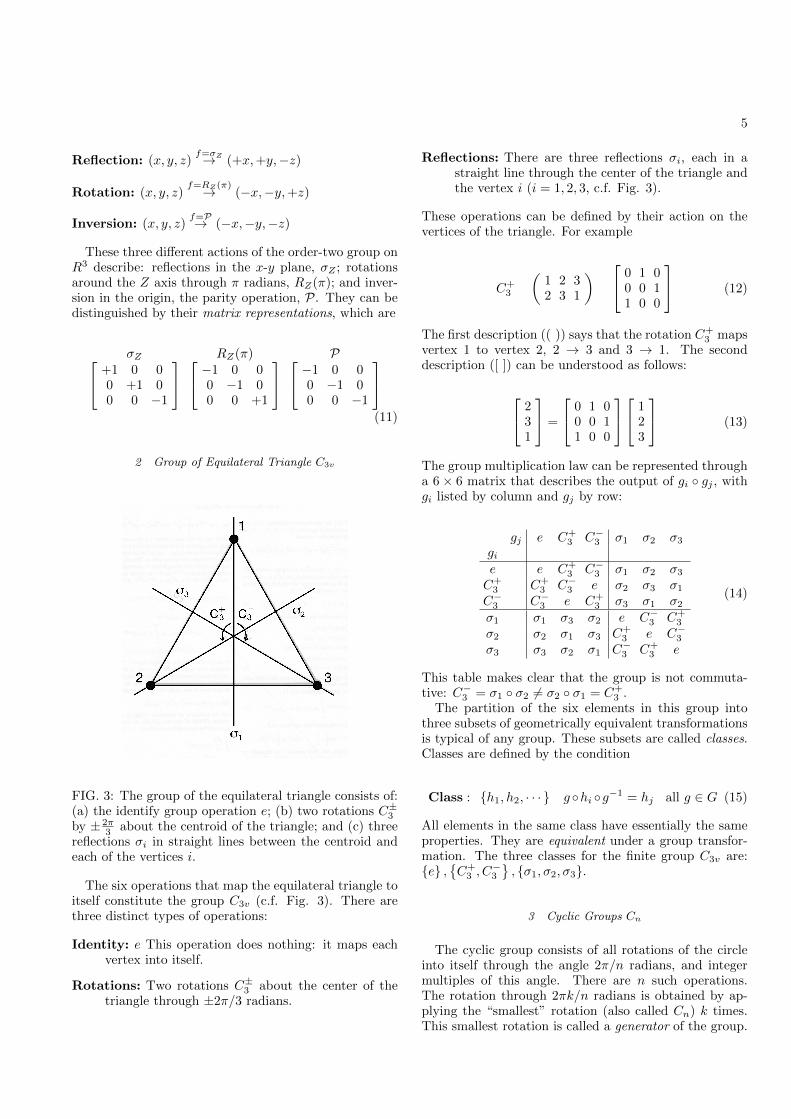
2 Group of Equilateral Triangle C3v

FIG. 3: The group of the equilateral triangle consists of:(a) the identify group operation e; (b) two rotations C±3by ± 2π

3 about the centroid of the triangle; and (c) threereflections σi in straight lines between the centroid andeach of the vertices i.

The six operations that map the equilateral triangle toitself constitute the group C3v (c.f. Fig. 3). There arethree distinct types of operations:

Identity: e This operation does nothing: it maps eachvertex into itself.

Rotations: Two rotations C±3 about the center of thetriangle through ±2π/3 radians.

Reflections: There are three reflections σi, each in astraight line through the center of the triangle andthe vertex i (i = 1, 2, 3, c.f. Fig. 3).

These operations can be defined by their action on thevertices of the triangle. For example

C+3

(1 2 32 3 1

) 0 1 00 0 11 0 0

(12)

The first description (( )) says that the rotation C+3 maps

vertex 1 to vertex 2, 2 → 3 and 3 → 1. The seconddescription ([ ]) can be understood as follows:

231

=

0 1 00 0 11 0 0

123

(13)

The group multiplication law can be represented througha 6× 6 matrix that describes the output of gi gj , withgi listed by column and gj by row:

gj e C+3 C−3 σ1 σ2 σ3

gie e C+

3 C−3 σ1 σ2 σ3

C+3 C+

3 C−3 e σ2 σ3 σ1

C−3 C−3 e C+3 σ3 σ1 σ2

σ1 σ1 σ3 σ2 e C−3 C+3

σ2 σ2 σ1 σ3 C+3 e C−3

σ3 σ3 σ2 σ1 C−3 C+3 e

(14)

This table makes clear that the group is not commuta-tive: C−3 = σ1 σ2 6= σ2 σ1 = C+

3 .The partition of the six elements in this group into

three subsets of geometrically equivalent transformationsis typical of any group. These subsets are called classes.Classes are defined by the condition

Class : h1, h2, · · · g hi g−1 = hj all g ∈ G (15)

All elements in the same class have essentially the sameproperties. They are equivalent under a group transfor-mation. The three classes for the finite group C3v are:e ,

C+

3 , C−3

, σ1, σ2, σ3.

3 Cyclic Groups Cn

The cyclic group consists of all rotations of the circleinto itself through the angle 2π/n radians, and integermultiples of this angle. There are n such operations.The rotation through 2πk/n radians is obtained by ap-plying the “smallest” rotation (also called Cn) k times.This smallest rotation is called a generator of the group.

6

The group is commutative. There are therefore as manyclasses as group elements. The group operations can beput in 1 : 1 correspondence with the complex numbersand also with real 2× 2 matrices:

[ei2πk/n

]1×1← Ckn

2×2→[

cos 2πkn sin 2πk

n

− sin 2πkn cos 2πk

n

](16)

with k = 0, 1, 2 · · · , n − 1 or k = 1, 2, · · ·n. The groupelement, 1 × 1 complex matrix, 2 × 2 real matrix withk = 1 is the generator for the group, the 1 × 1 matrixrepresentation, and the 2× 2 matrix representation.

4 Permutation Groups Sn

Permutation groups act to interchange things. For ex-ample, if we have n numbers 1, 2, 3, · · ·n, each permuta-tion group operation will act to scramble the order of theintegers differently. Two useful ways to describe elementsin the permutation group are shown in Eq. (12) for thepermutation group on three vertices of an equilateral tri-angle. In the first case, the extension of this notation forindividual group elements consists of a matrix with tworows, the top showing the ordering before the operation isapplied, the bottom showing the ordering after the groupoperation has been applied. In the second case shown inEq. (12) the extension consists of n × n matrices withexactly one +1 in each row and each column. The order(number of group operations) of Sn is n!. Permutationgroups are noncommutative for n > 2. S3 = C3v.

The permutation group plays a fundamental role inboth mathematics and physics. In mathematics it is usedto label the irreducible tensor representations of all Liegroups of interest. In physics it is required to distinguishamong different states that many identical particles (ei-ther bosons or fermions) can assume.

websearch: permutation group, Hamermesh

C Infinite Discrete Groups

1 Translation Groups: 1 Dimension

Imagine a series of points at locations na along thestraight line, where a is a physical parameter with di-mensions of length ([a] = L) and n is an integer. Thegroup that leaves this set invariant consists of rigid dis-placements through integer multiples of the fundamentallength. The operation Tka displaces the point at na toposition (n+ k)a. This group has a single generator Ta,and Tka = Ta Ta · · · Ta = T ka . It is convenient torepresent these group operations by 2× 2 matrices

Tka →[

1 ka0 1

](17)

In this representation group composition is equivalent tomatrix multiplication. The group is commutative. Thegenerator for the group and this matrix representation isobtained by setting k = 1. There is also an entire setof 1 × 1 complex matrix representations with generatorTa →

[eipa

]. The representations with p′ = p+ 2π/a are

equivalent, so all the inequivalent complex representa-tions can be parameterized by real values of p in the range0 ≤ p < 2π/a or, more symmetrically −π/a ≤ p ≤ π/a,with the endpoints identified. The real parameter p isin the dual space to the lattice, called the first Brillouinzone.

2 Translation Groups: 2 Dimensions

Now imagine a series of lattice points in a plane atpositions x = i1f1 + i2f2. Here i1, i2 are integers andthe vectors f1, f2 are not colinear but otherwise arbitrary.Then the set of rigid displacements (j1, j2) move latticepoints x to new locations as per

Tj1f1+j2f2 (i1f1 + i2f2) = (i1 + j1)f1 + (i2 + j2)f2 (18)

Generalizing Eq. (17), there is a simple 1 : 1 (or faithful)matrix representation for this group of rigid translations:

Tj1f1+j2f2 →

1 0 j1|f1|0 1 j2|f2|0 0 1

(19)

Extension to groups of rigid displacements of lattices inhigher dimensions is straightforward.

3 Spacegroups

When |f1| = |f2| and the two vectors are orthogonal,rotations through kπ/2 (k = 1, 2, 3) radians about anylattice point map the lattice into itself. So also do re-flections in lines perpendicular to |f1| and |f2| as well aslines perpendicular to ±|f1|±|f2|. This set of group oper-ations contains displacements, rotations, and reflections.It is an example of a two-dimensional space group. Thereare many other space groups in two dimensions and verymany more in three dimensions. These groups were firstused to enumerate the types of regular lattices that Na-ture allows in two and three dimensions. After the devel-opment of Quantum Mechanics they were used in anotherway (depending of the theory of representations): to givenames to wavefunctions that describe electrons (and alsophonons) in these crystal lattices.

7

D Matrix Groups

1 Translation Groups

The group of rigid translations of points in R3 throughdistances a1 in the x-direction, a2 in the y-direction, anda3 in the z-direction can be described by simple block4× 4 (4 = 3 + 1) matrices:

Ta1,a2,a3 →

1 0 0 a1

0 1 0 a2

0 0 1 a3

0 0 0 1

(20)

If the a belong to a lattice the group is discrete. If theyare continuous (a = (x, y, z)) the group is continuous andhas dimension three.

2 Heisenberg Group H3

The Heisenberg group H3 plays a fundamental rolein quantum mechanics. As it appears in the quantumtheory it is described by “infinite-dimensional” matrices.However, the group itself is three dimensional. In fact, ithas a simple faithful description in terms of 3×3 matricesdepending on three parameters:

h(a, b, c) =

1 a c0 1 b0 0 1

(21)

The group is not commutative. The group multiplicationlaw can be easily worked out via matrix multiplication:

h1h2 = h3 = h(a3, b3, c3) =

1 a1 + a2 c2 + a1b20 1 b1 + b20 0 1

(22)

The result c3 = a1b2 +c2 leads to remarkable noncommu-tativity properties among canonically conjugate variablesin the quantum theory: [p, x] = ~/i.

3 Rotation Group SO(3)

The set of rigid rotations of R3 into itself forms agroup. It is conveniently represented by a faithful 3 × 3matrix. The 3 × 3 matrix describing rotations about anaxis of unit length n through an angle θ, 0 ≤ θ ≤ π is

(n, θ)→ I3 cos θ+n · L sin θ+

n1

n2

n3

×[ n1 n2 n3

](1−cos θ)

(23)

Here L is a set of three 3×3 angular momentum matrices

Lx =

0 0 00 0 10 −1 0

Ly =

0 0 −10 0 01 0 0

Lz =

0 1 0−1 0 00 0 0

(24)

We will show later how this marvelous expression hasbeen derived.

There is a 1:1 correspondence between points in theinterior of a sphere of radius π and rotations throughan angle in the range 0 ≤ θ < π. Two points on thesphere surface (n, π) and (−n, π) describe the same rota-tion. The parameter space describing this group is not asimply connected submanifold of R3: it is a doubly con-nected manifold. The relation between continuous groupsand their underlying parameter space involves some fas-cinating topology.

4 Lorentz Group SO(3, 1)

The Lorentz group is the group of linear transforma-tions that leave invariant the square of the distance be-tween two nearby points in spacetime: (cdt, dx, dy, dz)and (cdt′, dx′, dy′, dz′). The distance can be written inmatrix form:

(cdτ)2 = (cdt)2 − (dx2 + dy2 + dz2) =

[cdt dx dy dz

] +1 0 0 00 −1 0 00 0 −1 00 0 0 −1

cdtdxdydz

(25)

If the infinitesimals in the primed coordinate system arerelated to those in the unprimed coordinate system bya linear transformation — dx

′µ = Mµν dx

ν — then thematrices M must satisfy the constraint (t means matrixtranspose)

M tI1,3M = I1,3 (26)

where I1,3 is the diagonal matrix diag(+1,−1,−1,−1).The matrices M belong to the orthogonal group O(1, 3).This is a six-parameter group. Clearly the rotations(three dimensions worth) form a subgroup, represented

by matrices of the form

[±1 00 ±R(n, θ)

], where R(n, θ)

is given in Eq.(23). This group has four disconnectedcomponents, each connected to a 4 × 4 matrix of the

form

[1 00 I3

],

[1 00 −I3

],

[−1 00 I3

],

[−1 00 −I3

]. We

choose the component connected to the identity I4. This

8

is the special Lorentz group SO(1, 3). A general matrixin this group can be written in the form

SO(1, 3) = B(β)R(θ) (27)

where the matrices B(β) describe boost transformations.A boost transformation maps a coordinate system at restto a coordinate moving with velocity v = cβ and withaxes parallel to the stationary coordinate system. Wewill describe these transformations in more detail below.

Since every group operation in SO(1, 3) can be ex-pressed as the product of a rotation operation with aboost, we can formally write B(β) = SO(1, 3)/SO(3).In fact, such an expression makes sense in this case. Asimilar result makes sense for any group G and subgroupH ⊂ G. Every element g ∈ G can be expressed asthe product of an h ∈ H and another group operationc ∈ G. In fact, it is a theorem that the set c belongs toa small subset C ⊂ G called a coset. For finite groups,|C| = |G|/|H|. That is, the order, or number of elementsin C, is equal to the number of elements in G divided bythe number of elements in the subgroup H. For infiniteand continuous groups something similar holds (in thesense of dimensions or measures). Such a decomposition,generally written

Coset Decomposition G = (G/H)·H = C ·H (28)

is called a coset decomposition. In general, the set ofgroup elements in C do not satisfy the axioms for agroup. Not all coset decompositions carry as much phys-ical sense as the boost - rotation decomposition of theLorentz group.

A general boost transformation can be written in theform

B(β) =

[γ γβ

γβ I3 + (γ − 1)βiβjβ·β

](29)

For example, a boost with v/c = (β, 0, 0) has the follow-ing effect on coordinates:

ctxyz

′

=

γ γβ 0 0γβ γ 0 00 0 1 00 0 0 1

ctxyz

=

γ(ct+ βx)γ(x+ βct)

yz

(30)

Here γ2 − (βγ)2 = 1 so γ = 1/√

1− β2. In the non-relativistic limit x′ = γ(x + βct) → x + vt, so β has aninterpretation of β = v/c.

The product of two boosts in the same direction isobtained by matrix multiplication. This can be carriedout on a 2× 2 submatrix of that given in Eq. (30):

B(β1)B(β2) =

[γ1 β1γ1

β1γ1 γ1

] [γ2 β2γ2

β2γ2 γ2

]=

[γtot βtotγtot

βtotγtot γtot

] (31)

Simple matrix multiplication shows βtot = β1+β2

1+β1β2, which

is the relativistic velocity addition formula for parallelvelocity transformations.

When the boosts are not parallel, their product is atransformation in SO(1, 3) that can be written as theproduct of a boost with a rotation:

B(β1)B(β2) = B(βtot)R(θ) (32)

Multiplying two boost matrices of the form given inEq. (29) leads to a simple expression for γtot and a morecomplicated expression for βtot

γtot = γ1γ2(1 + β1 · β2)

γtotβtot =[γ1γ2 + (γ1 − 1)γ2

β1·β2

β1·β1

]β1 + γ2β2

(33)

This shows what is intuitively obvious: the boost direc-tion is in the plane of the two boosts. Less obvious is therotation required by noncollinear boosts. It is around anaxis parallel to the crossproduct of the two boosts. Whenthe two boosts are perpendicular the result is

n sin(θ) = −β1 × β2 ·γ1γ2

1 + γ1γ2(34)

When one of the boosts is infinitesimal we find

B(β)B(δβ) = B(β + dβ)R(ndθ) (35)

Multiplying out these matrices and comparing the twosides gives:

dβ = γ−1δβ +

(γ−1 − 1

γβ2

)(β · δβ)β

ndθ =

(1− γ−1

β2

)δβ × β

(36)

In the nonrelativistic limit, when β is also small, 1 −γ−1/β2 → 1

2 . This (in)famous factor of 1/2 is known asthe “Thomas factor” in atomic physics.

websearch: Lorentz group, boost, rotationwebsearch: Thomas precession

9

E Lie Groups

The group operations g in a Lie group are parame-terized by points x in a manifold Mn of dimension n:g = g(x), x ∈ Mn. The product of two group opera-tions g(x) and g(y) is parameterized by a point z in themanifold: g(x) g(y) = g(z), where z = z(x,y). Thiscomposition law can be very complicated. It is necessar-ily nonlinear unless the group is commutative (c.f., Eq.(22) for H3).

Almost all of the Lie groups of use to physicists existas matrix groups. For this reason it is possible for us toskip over the fundamental details of whether the com-position law must be analytic and the elegant details oftheir definition and derivations. We list several types ofmatrix groups below.

GL(n;R), GL(n;C), GL(n;Q): These groups consistof n× n matrices, each of whose n2 matrix elements arereal numbers, complex numbers, or quaternions. In orderfor inverses to exist, noninvertible matrices do not occurin these matrix groups. The number of real parametersrequired to specify an element in these groups is: n2, 2×n2, 4× n2.

SL(n;R), SL(n;C): These groups are subgroups ofGL(n;R) and GL(n;C) containing the subset of matri-ces with determinant +1. The real dimensions of thesegroups are (n2 − 1)× dim(F ) where dim(F ) = (1, 2) forF = (R,C).

O(n), U(n), Sp(n): Three important classes ofgroups are defined by placing quadratic constraints onmatrices. The orthogonal group O(n) is the subgroupof GL(n;R) containing only matrices M that satisfyM tInM = In. Here In is the unit n×n matrix and t sig-nifies the transpose of the matrix. This constraint arisesin a natural way when requiring that linear transforma-tions in a real n-dimensional linear vector space preservea positive definite inner product. The unitary groupU(n) is the subgroup of GL(n;C) for which the matricesM satisfy M†InM = In, where † signifies the adjoint,or complex conjugate transpose matrix. The symplecticgroup Sp(n) is defined similarly for the quaternions. Inthis case † signifies quaternion conjugate transpose. Thereal dimensions of these groups are n(n − 1)/2, n2, andn(2n+ 1), respectively.

SO(n), SU(n): The “S” stands for special and specialmeans the determinant is +1. For the group O(n) the de-terminant of any group operation is a real number whosemodulus is +1: i.e., ±1. Placing the special constrainton the group of orthogonal transformations reduces the“number” of elements in the group by one half (in a mea-sure theoretic sense) but does not reduce the dimensionof the space required to parameterize the elements in thisgroup. For the group U(n) the determinant of any groupoperation is a complex number whose modulus is +1: i.e.,eiφ. Placing the special constraint on U(n) reduces thedimension by one: dim SU(n) = n2 − 1. The symplecticgroup Sp(n) has determinant +1.

O(p,q), U(p,q), Sp(p,q): These groups are definedby replacing In in the definitions for O(n), U(n), Sp(n) by

the matrix Ip,q =

[+Ip 0

0 −Iq

]. These groups preserve

an indefinite nonsingular metric in linear vector spacesof dimension (p + q). The groups O(n), U(n), Sp(n) arecompact (a useful topological concept) and so are rel-atively easy to deal with. This means effectively thatonly a finite volume of parameter space is required toparameterize every element in the group. The groupsO(p, q), U(p, q), Sp(p, q) are not compact if both p andq are nonzero. Further, O(p, q) ' O(q, p) by a simplesimilarity transformation, and similarly for the others.

websearch: Lie groups of matrices

F Lie Algebras

Lie algebras are constructed for a Lie group by lineariz-ing the Lie group in the neighborhood of the identity e.Matrix Lie algebras are obtained for n × n matrix Liegroups by linearizing the matrix group in the neighbor-hood of the unit matrix In. A Lie group and its Liealgebra have the same dimension.

In the neighborhood of the identity the groupsGL(n;R), GL(n;C), GL(n,Q) have the form

GL(n;F )→ In + δM (37)

where δM is an n×n matrix, all of whose matrix elementsare small. Over the real, complex, and quaternion fieldsthe matrix elements are small real or complex numbersor small quaternions. Quaternions q can be expressed as2× 2 complex matrices using the Pauli spin matrices σµ:

q → (c0, c1) = (r0, r1, r2, r3) =

3∑µ=0

rµσµ =

[r0 + ir3 r1 − ir2

r1 + ir2 r0 − ir3

](38)

The Lie algebras gl(n;F ) of GL(n;F ) have dimensionsf × n2, f = 1, 2, 4 for F = R,C,Q.

For the special linear groups, the determinant is

det(In + δM) = 1 + trδM + h.o.t. (39)

The Lie algebras are defined by the traceless condition.The Lie algebra sl(n;R) of SL(n;R) consists of real trace-less n × n matrices. It has dimension n2 − 1. The Liealgebra sl(n;C) of SL(n;C) consists of traceless complexn× n matrices. It has real dimension 2n2 − 2.

Many Lie groups are defined by a metric-preservingcondition: M†GM = G, where G = is some suitable

10

metric matrix (see Sec. III E). The linearization of thiscondition is

M†GM → (In+δM)†G(In+δM) = G+δM†G+GδM

+h.o.t = G⇒ δM†G + GδM = 0 (40)

When G is the identify matrix, the lie algebrasso(n;R), su(n;C), sp(n;Q) consists of real antisymmet-ric matrices M t = −M , complex traceless antihermitianmatrices M† = −M , and quaternion antihermitian ma-trices M† = −M , respectively.

The elements in a Lie group must obey one single groupmultiplication law. The elements in the group’s Lie al-gebra have simpler properties, as they are obtained bylinearization about the identity group operation. In or-der to reflect the nonlinear group multiplication proper-ties they must satisfy more conditions. Construction bylinearization means that the Lie algebra is a linear vec-tor space. If X and Y are elements in a Lie algebra,αX + βY is also in the Lie algebra. Here α and β arearbitrary real scalars. Closure under multiplication inthe group leads to the requirement that the commuta-tor [X,Y ] = XY − Y X = − [Y,X] is also an element inthe Lie algebra. There is only one other condition thatthe elements in a Lie algebra are required to satisfy: theJacobi identity:

[X, [Y, Z]] + [Y, [Z,X]] + [Z, [X,Y ]] = 0 (41)

For matrix Lie algebras this relation is indeed an identity,but for abstract Lie algebras where composition XY isnot naturally defined, the commutator [X,Y ] is alwaysdefined, and the identity is satisfied.

The Lie algebra so(3) of the rotation group SO(3) =SO(3;R) consists of real 3 × 3 antisymmetric matrices.This group and its algebra are three dimensional. The Liealgebra (it is a linear vector space) is spanned by three“basis vectors”. These are 3× 3 antisymmetric matrices.A standard choice for these basis vectors is given in Eq.(24). Their commutation relations are given by

[Li, Lj ] = −εijkLk (42)

More generally, for an arbitrary n-dimensional Lie alge-bra it is possible to choose a set of n basis vectors (ma-trices, operators) Xi. The commutation relations are en-capsulated by a set of structure constants Ckij that aredefined by

[Xi, Xj ] = CkijXk (43)

The structure constants for so(3) are Ckij = −εijk, 1 ≤i, j, k ≤ 3.

Two Lie algebras with the same set of structure con-stants are isomorphic. The Lie algebra of 2× 2 matricesobtained from su(2) is spanned by three operators thatcan be chosen as proportional ( i2 ) to the Pauli spin ma-trices (c.f., Eq. (38)):

S1 =i

2

[0 11 0

]S2 =

i

2

[0 −i

+i 0

]S3 =

i

2

[1 00 −1

](44)

These three operators satisfy the commutation relations

[Si, Sj ] = −εijkSk (45)

As a result, the Lie algebra for the group so(3) of ro-tations in R3 is isomorphic to the Lie algebra su(2) forthe group of unimodular metric-preserving rotations ina complex two dimnensional space, SU(2). Spin and or-bital rotations are intimately connected.

The notation for the structure constants Ckij for a Liealgebra gives the appearance of being components of atensor. In fact, they are: the tensor is first order con-travariant (in k) and second order covariant, and anti-symmetric, in i, j. It is possible to form a second ordercovariant tensor (Cartan-Killing metric) from the com-ponents of the structure constant by double contraction:

gij =∑rs

CsirCrjs = gji (46)

This real symmetric tensor “looks like” a metric tensor.In fact, it has very powerful properties. If g∗∗ is non-singular the Lie algebra, and its Lie group, is “simple”or “semisimple”. If g∗∗ is negative definite, the group iscompact. It is quite remarkable that an algebraic struc-ture gives such powerful topological information.

As an example, for SO(3) and SU(2) the Cartan-Killing metric Eq. (46) is

gij =∑r,s

(−εirs)(−εjsr) = −δij (47)

For the real forms SO(2, 1) of SO(3) and SU(1, 1) ofSU(2) the Cartan-Killing metric tensor is

g ((so(2, 1), su(1, 1)) =

+1 0 00 +1 00 0 −1

(48)

The structure of this metric tensor (two positive diagonalelements or eigenvalues, and one negative) tells us aboutthe topology of the groups: they have two noncompact di-rections and one compact direction. The compact direc-tion describes the compact subgroups SO(2) and U(1),respectively.

websearch: Lie groups Lie algebraswebsearch: EXPonential map Lie algebras

11

G Operator Realizations of Lie Algebras

Each Lie algebra has three useful operator realizations.They are given in terms of boson operators, fermion op-erators, and differential operators.

Boson annihilation operators bi and creation operators

b†j for independent modes i, j = 1, 2, · · · , their fermion

counterparts fi, f†j , and the operators ∂i, xj satisfy the

following commutation or anticommutation relations

[bi, b

†j

]= bib

†j − b

†jbi = δij

fi, f†j

= fif

†j + f†j fi = δij

[∂i, xj ] = ∂ixj − xj∂i = δij

(49)

In spite of the fact that bosons and differential opera-tors satisfy commutation relations and fermion operatorssatisfy anticommutation (see the + sign in Eq. (49)) re-

lations, bilinear combinations Zij = b†i bj , f†i fj , xi∂j of

these operators satisfy commutation relations:

[Zij , Zrs] = Zisδjr − Zrjδsi (50)

These commutation relations can be used to associateoperator algebras to matrix Lie algebras. The procedureis simple. We illustrate for boson operators. AssumeA,B,C = [A,B] are n×n matrices in a matrix Lie alge-bra. Associate operator A to matrix A by means of

A→ A = b†iAijbj (51)

and similarly for other matrices. Then

[A,B] =[b†iAijbj , b

†rBrsbs

]= b†i [A,B]is bs = b†iCisbs = C

(52)This result holds if the bilinear combinations of bosoncreation and annihilation operators are replaced by bi-linear combinations of fermion creation and annihilationoperators or products of multiplication (by xi) and dif-ferentiation (by ∂j) operators.

One consequence of this matrix Lie algebra to operatoralgebra isomorphism is that any Hamiltonian that can beexpressed in terms of bilinear products of creation andannihilation operators for either bosons or fermions canbe studied in a simpler matrix form.

The operator algebra constructed from the spin op-erators in Eq. (44) has been used by Schwinger for anelegant construction of all the irreducible representationsof the Lie group SU(2) (c.f., Sec. V E and Fig. 4).

We use the matrix-to-operator mapping now to con-struct a differential operator realization of the Heisenberggroup, given in Eq. (21). Linearizing about the identifygives a three-dimensional Lie algebra of the form

0 l d0 0 r0 0 0

= lL+ rR+ dD (53)

Here L,R,D are 3× 3 matrices. The only nonzero com-mutator is [L,R] = D. The corresponding differentialoperator algebra is

[x y z

] 0 l d0 0 r0 0 0

∂x∂y∂z

= lL+ rR+ dD (54)

The three differential operators are

L = x∂y R = y∂z D = x∂z (55)

Among these operators: none depends on z (so ∂z hasnothing to operate on) and none contains ∂x, so that inessence x is an irrelevant variable. A more economicalrepresentation of this algebra is obtained by zeroing outthe cyclic variables z, ∂x and replacing their conjugatevariables ∂z, x by +1.

[1 y 0

] 0 l d0 0 r0 0 0

0∂y1

= lL′ + rR′ + dD′ (56)

L′ = ∂y R′ = y D′ = 1 (57)

In essence, we have zeroed out the operators coupled tothe vanishing rows and columns of the matrix Lie alge-bra and replaced their conjugate variables by 1. Therepresentation given is essentially the Hiesenberg repre-sentation of the position (y) and conjugate momentum(py ' ∂y) operators in Quantum Mechanics.

websearch: Lie algebra operator algebra mapping

H Exponentiation

The mapping of a Lie group, with a complicated non-linear composition, down to a Lie algebra with a simplelinear combinatorial structure plus a commutator, wouldnot be so useful if it were not possible to undo this map-ping. In effect, the linearization is “undone” by the ex-ponential map. For an operator X the exponential isdefined in the usual way:

EXP (X) = eX = I+X+X2

2!+X3

3!+· · · =

∞∑k=0

Xk

k!(58)

The radius of convergence of the exponential function isinfinite. This means that we can map a Lie algebra backto its parent Lie group in an algorithmic way.

12

We illustrate with two important examples. For thefirst, we construct a simple parameterization of the groupSU(2) by exponentiating its Lie algebra. The Lie alge-bra is given in Eq. (44). Define M = i

2 n · σθ. Then

M2 = −(θ/2)2I2 is a diagonal matrix. The exponentialexpansion can be rearranged to contain even powers inone sum and odd powers in another:

eM = I2

(1− (θ/2)2

2!+

(θ/2)4

4!− · · ·

)+

M

(1− (θ/2)2

3!+

(θ/2)4

5!− · · ·

)(59)

The even terms sum to cos(θ/2) and the odd terms sumto sin(θ/2)/(θ/2). The result is

EXP

(i

2n · σθ

)= cos

θ

2I2 + in · σ sin

θ

2(60)

A similar power series expansion involving the angularmomentum matrices in Eq. (24) leads to the parameteri-zation of the rotation group operations given in Eq. (23).Specifically, EXP (n · Lθ) =

I3 cos θ + n · L sin θ +[n1 n2 n3

] n1

n2

n3

(1− cos θ)

(61)The Lie groups SO(3) and SU(2) possess isomorphic

Lie algebras. The Lie algebra is three-dimensional. Thebasis vectors in so(3) can be chosen as the angular mo-mentum matrices given in Eq. (24) and the basis vectorsfor su(2) as i/2 times the Pauli spin matrices, as in Eq.(44). A point in the Lie algebra (e.g., R3) can be iden-tified by a unit vector n and a radial distance from theorigin θ. Under exponentiation, the point (n, θ) maps tothe group operation given in Eq. (61) for SO(3) and inEq. (60) for SU(2).

The simplest way to explore how the Lie algebra pa-rameterizes the two groups is to look at how points alonga straight line through the origin of the Lie algebra mapto operations in the two groups. For simplicity we choosethe z-axis. Then (z, θ) maps to

[eiθ/2 0

0 e−iθ/2

]∈ SU(2),

cos θ sin θ 0− sin θ cos θ 0

0 0 1

∈ SO(3)

(62)As θ increases from 0 to 2π the SU(2) group operationvaries from +I2 to −I2 while the SO(3) group opera-tion starts at I3 and returns to +I3. The SU(2) groupoperation returns to the identity +I2 only after θ in-creases from 2π to 4π. The rotations by θ and θ + 2π

give the same group operation in SO(3) but they de-scribe group operations in SU(2) that differ by sign:(z, 2π+ θ) = −I2× (z, θ). In short, two group operationsM and −M in SU(2) map to the same group oprationin SO(3). In words, SU(2) is a double cover of SO(3).

For SU(2) all points inside a sphere of radius 2π in theLie albegra map to different group operations, and allpoints on the sphere surface map to one group operation−I2. The group SU(2) is simply connected. Any pathstarting and ending at the same point (for example, theidentity) can be continuously contracted to the identity.

By contrast, for SO(3) all points inside a sphere ofradius π in the Lie algebra map to different group opera-tions, and two points (n, π) and −(n, π) at opposite endsof a straight line through the origin map to the samegroup operation. The group SO(3) is not simply con-nected. Any closed path from the origin that cuts thesurface θ = π once (or an odd number of times) can-not be continuously deformed to the identity. The groupSO(3) is doubly connected.

This is the simplest example of a strong theorem byCartan. There is a 1 : 1 relation between Lie algebras andsimply connected Lie groups. Every Lie group with thesame (isomorphic) Lie algebra is either simply connectedor else the quotient (coset) of the simply connected Liegroup by a discrete invariant subgroup.

For matrix Lie groups, discrete invariant subgroupsconsist of scalar multiples of the unit matrix. Forthe the isomorphic Lie algebras su(2) = so(3) the Liegroup SU(2) is simply connected. Its discrete invari-ant subgroup consists of multiples of the identity ma-trix: I2,−I2. Cartan’s theorem states SO(3) =SU(2)/ I2,−I2. This makes explicit the 2 ↓ 1 natureof the relation between SU(2) and SO(3).

The group SU(3) is simply connected. It discrete in-variant subgroup consists of

I3, ωI3, ω

2I3

, with ω3 = 1.The only other Lie group with the Lie algebra su(3) isthe 3 ↓ 1 image SU(3)/

I3, ωI3, ω

2I3

. This group hasa description in terms of real eight dimensional matrices(“the eightfold way”).

websearch: EXP Lie algebra Lie group

I Riemannian Symmetric Spaces

The Lie algebra for the Lorentz group consists of 4× 4matrices:

so(1, 3) =

0 α1 α2 α3

α1 0 θ3 −θ2

α2 −θ3 0 θ1

α3 θ2 −θ1 0

(63)

The Cartan-Killing metric for SO(1, 3) is

g(so(1, 3), so(1, 3)) = α21 + α2

2 + α23 − θ2

1 − θ22 − θ2

3 (64)

13

The subalgebra of rotations so(3) describes the compactsubgroup SO(3). The remaining three infinitesimal gen-erators parameterized by αi span the noncompact part ofthis group, the coset SO(1, 3)/SO(3), and exponentiateto boost operations.

Cartan has pointed out that it is often possible to de-compose the Lie algebra g for Lie group G into two com-plementary subspaces: k, which exponentiates to a sub-group K ⊂ G; and a complementary subspace p, wherethe two subspaces satisfy these commutation relations:

[k, k] ⊆ k [k, p] ⊆ p [p, p] ⊆ k (65)

When this is possible, EXP (p) = P = G/K. Further, ifthe Cartan-Killing metric is negative definite on k, andpositive definite on p, then K is a maximal compact sub-group of G and the coset P = G/K is a Riemanniansymmetric space. For the Lorentz group SO(1, 3), byCartan’s criterion SO(3) is the maximal compact sub-group and the coset of boost transformations B(β) =SO(1, 3)/SO(3) is a three-dimensional Riemannian spacewith positive-definite metric. In this case the space is a3-hyperboloid (ct)2 − x2 − y2 − z2 = cst. embedded inR4. The metric on this space is obtained by moving themetric (1, 1, 1) at the origin (x, y, z) = (0, 0, 0) over theembedded space using the set of Lorenz group transfor-mations in the quotient space SO(1, 3)/SO(3). Cartanalso showed that all Riemannian symmetric spaces ariseas quotients of (simple) Lie groups by maximal compactsubgroups.

websearch: Riemannian symmetric spaces, Car-tan

J Disentangling Results

It happens surprisingly often in distantly related fieldsof physics that expressions of the form ex+∂x are encoun-tered. Needless to say, these are not necessarily endear-ing to work with. One approach to simplifying computa-tions involving such operators is to rewrite the operatorin such a way that all differential operators ∂x act first,and all multiplications by x act last. One way to effectthis decomposition is to cross one’s fingers and write thisoperator as eax+b∂x ' eaxeb∂x and hope for the best. Ofcourse this doesn’t work, since the operators x and ∂x donot commute.

Exponential operator rearrangements are called disen-tangling theorems. Since the exponential mapping is in-volved, powerful methods are available when the opera-tors in the exponential belong to a finite-dimensional Liealgebra. Here is the algorithm:

1. Determine the Lie algebra.2. Find a faithful finite-dimensional matrix represen-

tation of this Lie algebra.3. Identify how you want the operators ordered in the

final product of exponentials.

4. Compute this result in the faithful matrix represen-tation.

5. Lift this result back to the operator form.We now show how this algorithm works. The opera-

tors x and ∂x have one nonzero commutator [∂x, x] = 1.These three operators close under commutation. Theytherefore form a Lie algebra. This is the algebra h3 ofthe Heisenberg group, Eq. (57). We also have a faithfulmatrix representation of this Lie algebra, given in Eq.(56). We then make the identification

eax+b∂x → EXP

0 b 00 0 a0 0 0

=

1 b ab2

0 1 a0 0 1

(66)

Now we identify this matrix with

erxedIel∂x →

1 0 00 1 r0 0 1

1 0 d0 1 00 0 1

1 l 00 1 00 0 1

(67)

By multiplying out the three matrices in Eq. (67) andcomparing with the matrix elements of the 3× 3 matrixin Eq. (66) we learn that l = b, r = a, d = ab

2 . Portingthe results of this matrix calculation back to the land ofoperator algebras, we find

eax+b∂x = eaxeab2 eb∂x (68)

We will use this expression in Sec. IX G below to con-struct a generating function for the Hermite polynomials.

websearch: Lie group disentangling theorems

IV. APPLICATIONS IN CLASSICAL PHYSICS

Group Theory’s first important role in physics cameeven before Quantum Mechanics was discovered. Thetwo pillars of classical deterministic physics are Mechan-ics and Electrodynamics. Group Theory played a fun-damental role in rectifying the difficulties in describingthe interactions between these two fields. The principletool used, besides Group Theory, was Galileo’s Princi-ple of Relativity and an assumption about the undrlyingelegance of physical theories.

A Principle of Relativity

The Principle of Relativity posits: Two observers, Sand S′, observe the same physical system. Each knowshow his coordinate system is related to the other’s —that is, the transformation of coordinates that maps onecoordinate system into the other. Assume both observerscollect data on the same physical system. Given the datathat S takes, and the coordinate transformation from S

14

to S′, S can predict the data that S′ has recorded. Andhe will be correct.

Essentially, without this ability to communicate dataamong observers, there would be little point in pursuingthe scientific method.

A second assumption that is used is usually not statedexplicitly. This assumption is: The quantitative formu-lation of physical laws is simple and elegant (whateverthat means).

websearch: Galileo relativity

B Mechanics and Electrodynamics

The quantitative formulation of Mechanics for a singleparticle in an inertial frame is

dp

dt= F(x) (69)

where p is defined by p = mdxdt . The transformations

from one inertial coordinate system to another consist of:displacements in space d, displacements in time d, Rigidrotations R, and boosts with constant velocity v thatkeep the axis parallel. The space and time coordinatesin S′ are related to those in S by

x′ = Rx + vt+ dt′ = t+ d

(70)

In inertial coordinate system S′ Newton’s equations are

dp′

dt= F′(x′)

x′ = Rxp′ = RpF′ = RF

(71)

The equations of motion have the same vectorial form inboth inertial coordinate systems (the simple and elegantassumption).

Newton’s Laws were incredibly successful in describingplanetary motion in our solar system, so when Maxwelldeveloped his laws for electrodynamics, it was natural toassume that they also retained their form under the setof inertial coordinate transformations given in Eq. (70).Applying these transformations to Maxwell’s equationscreates a big mess. But if one looks only at signals prop-agating along or opposite the direction of the velocity v,these assumptions predict

(c dt)′ → c′ dt c′ = c± |v| (72)

The round trip time for a light signal in S is 2L/c while in

S′ the time lapse was predicted to be Lc+v + L

c−v = 2L/c1−β2 ,

with β = |v|/c.This predicted difference in elapsed round trip times

in ‘rest’ and ‘moving’ frames was thought to enable us to

determine how fast the earth was moving in the Universe.As ever more precise measurements in the late nineteenthand early twentieth century lead to greater disappoint-ment, more and more bizarre explanations were createdto ‘explain’ this null result. Finally Einstein and Poincarereturned to the culprit Eq.(72) and asserted what the ex-periments showed: c′ = c, so that

(c dt)′ → c dt′ dt′ = linear comb. dx, dy, dz, dt (73)

The condition that the distance function

(c dτ)2 = (c dt)2 − (dx2 + dy2 + dz2) =(c dt′)2 − (dx′2 + dy′2 + dz′2)

(74)

is invariant leads directly to the transformation law forinfinitesimals dx′µ = Λµνx

ν , where the 4× 4 matrices be-

long to the Lorentz group Λ ∈ SO(3, 1), Λµν = ∂x′µ/∂xν .

The transformation laws taking inertial frames S to iner-tial frames S′ involves inhomogeneous coordinate trans-formations

[x′

1

]=

[SO(3, 1) d

0 1

] [x1

](75)

While Maxwell’s equations remain unchanged in formunder this set of coordinate transformations (inhomoge-neous Lorentz group), Newton’s force law no longer pre-serves its form.

In order to find the proper form for the laws of classi-cal mechanics under this new set of transformations thefollowing two-step process was adopted:

1. Find an equation that has the proper transforma-tion properties under the inhomogeneous Lorentzgroup;

2. If the equation reduces to Newton’s equation of mo-tion in the nonrelativistic limit β → 0 it is theproper generalization of Newton’s equation of mo-tion.

Appliction of the procedure leads to the relativistic equa-tion for particle motion

dpµ

dτ= fµ (76)

where pµ is defined by pµ = mdxµ

dτ . The components ofthe relativistic four vector fµ are related to the three-vector force F by

f = F + (γ)β · Fβ · β

β

f0 = γβ · F(77)

(c.f., Eq. (29)).

15

C Gravitation

Einstein wondered how it could be possible to deter-mine if you were in an inertial frame. He decided that thealgorithm for responding to this question, Newton’s FirstLaw (In an inertial frame, an object at rest remains atrest and an object in motion remains in motion with thesame velocity unless acted upon by external forces.) wascircularly defined (How do you know there are no forces?When you are sufficiently far away from the fixed stars.How do you know you are sufficiently far away? Whenthere are no forces.)

He therefore set out to formulate the laws of mechanicsin such a way that they were invariant in form under anarbitrary coordinate transformation. While the Lorentzgroup is six dimensional, general coordinate transforma-tions form an “infinite dimensional” group. The transfor-mation properties at any point are defined by a Jacobian

matrix[∂x′µ

∂xν (x)]. Whereas for the Lorentz this matrix is

constant throughout space, for general coordinate trans-formations this 4× 4 matrix is position dependent.

Nevertheless, he was able to modify the algorithm de-scribed above to formulate laws that are invariant underall coordinate transformations. This two-step process isa powerful formulation of the Equivalence Principle. It iscalled the Principle of General Covariance. It states thata law of physics holds in the presence of a gravitationalfield provided:

1. The equation is invariant in form under an arbitrarycoordinate transformation x→ x′(x).

2. In a locally free-falling coordinate system, or theabsence of a gravitational field, the equation as-sumes the form of a law within the Special Theoryof Relativity.

Using these arguments, he was able to show that theequation describing the trajectory of a particle is

d2xµ

dτ2= −Γµν,κ

dxν

dτ

dxκ

dτ(78)

The Christoffel symbols are defined in terms of the metrictensor gµ,ν(x) by

Γµν,κ =1

2gµ,ρ

(∂gν,ρ∂xκ

+∂gρ,κ∂xν

− ∂gν,κ∂xρ

)(79)

They are not components of a tensor, as coordinatesystems can be found (freely falling, as in an elevator) inwhich they vanish and the metric tensor reduces to itsform in Special Relativity form g = diag(1,−1,−1,−1).

Neither the left hand side nor the right hand side ofEq. (78) is invariant under arbitrary coordinate changes(extra terms creep in), but the following transformationlaw is valid:

d2x′µ

dτ2+Γ

′µν,κ

dx′ν

dτ

dx′κ

dτ=

(∂x

′µ

∂xλ

)(d2xλ

dτ2+ Γλν,κ

dxν

dτ

dxκ

dτ

)(80)

This means that the set of terms on the left, or thosewithin the brackets on the right, have the simple transfor-mation properties of a four-vector. In a freely falling co-ordinate system the Christoffel symbols vanish and what

remains is d2xλ

dτ2 . This Special Relativity expression is zeroin the absence of forces, so the equation that describesthe trajectory of a particle in a gravitational field is

d2xλ

dτ2+ Γλν,κ

dxν

dτ

dxκ

dτ= 0 (81)

D Reflections

Two lines of reasoning have entered the reconciliationof the two pillars of classical deterministic physics andthe creation of a theory of gravitation. One is group the-ory and is motivated by Galileo’s Principle of Relativity.The other is more vague. It is a Principle of Elegance:there is the mysterious assumption that the structure ofthe “real” equations of physics are simple, elegant, andinvariant under a certain class of coordinate transforma-tions. The groups are the 10 parameter InhomogeneousLorentz Group in the case of the Special Theory of Rel-ativity and the much larger groups of general cordinatetransformations in the case of the General Theory of Rel-ativity. There is every liklihood that Martians from an-other galaxy will recognize the Principle of Relativity butno guarantee that their sense of simplicity and elegancewill be anything like our own.

V. LINEAR REPRESENTATIONS

The theory of representations of groups — more pre-cisely the linear representations of groups by matrices —was actively studied by mathematicians while physicistsactively ignored these results. This picture changed dra-matically with the development of the Quantum Theory,the understanding that the appropriate “phase space”was the Hilbert space describing a quantum system, andthat group operations acted in these spaces through theirlinear matrix representations.

A linear matrix representation is a mapping of groupelements g to matrices g → Γ(g) that preserves the groupoperation:

gi gj = gk ⇒ Γ(gi)× Γ(gj) = Γ(gk) (82)

Here is the composition in the group and × indicatesmatrix multiplication. Often the mapping is one-way:

16

many different group operations can map to the samematrix. If the mapping is 1 : 1 the representation iscalled faithful.

A Maps to Matrices

We have already seen many matrix representations.We have seen representations of the two-element groupZ2 as reflection, rotation, and inversion matrices actingin R3 (c.f. Eq. (11)).

So: how many representations does a group have? Itis clear from the example of Z2 that we can create aninfinite number of representations. However, if we squintcarefully at the three representations presented in Eq.(11) we see that all these representations are diagonal:direct sums of essentially two distinct representations:

Z2 e fΓ1 1 1Γ2 1 −1

(83)

Each of the three matrix representations of Z2 in Eq. (11)is a direct sum of these two irreducible representations:

σZ = Γ1 ⊕ Γ1 ⊕ Γ2

RZ(π) = Γ1 ⊕ Γ2 ⊕ Γ2

P = Γ2 ⊕ Γ2 ⊕ Γ2(84)

A basic result of representation theory is that for largeclasses of groups (finite, discrete, compact Lie groups)every representation can be written as a direct sum ofthe special class of representations called irreducible rep-resentations. The procedure for constructing this directsum proceeds by matrix diagonalization. Irreducible rep-resentations are those that cannot be further diagonal-ized. In particular, one dimensional representations can-not be further diagonalized. Rather than enumeratingall possible representations of a group, it is sufficient toenumerate only the much smaller set of irreducible rep-resentations.

websearch: group representations

B Group Element - Matrix Element Duality

The members of a group can be treated as a set ofpoints. It then becomes possible to define a set of func-tions on this set of points. How many independent func-tions are needed to span this function space? A not tooparticularly convenient choice of basis functions are thedelta functions fi(g) = δ(g, gi). For example, for C3v

there are six group operations and therefore six basisfunctions for the linear vector space of functions definedon this group.

Each matrix element in any representation is a func-tion defined on the members of a group. It would seem

reasonable that the number of matrix elements in all theirreducible representations of a group provide a set of ba-sis functions for the function space defined on the set ofgroup operations. This is true: it is a powerful theorem.There is a far-reaching duality between the elements ina group and the set of matrix elements in its set of irre-ducible representations. Therefore if Γα(g), α = 1, 2, · · ·are the irreducible representations of a group G and thedimension of Γα(g) is dα (i.e., Γα(g) consists of dα × dαmatrices), then the total number of matrix elements isthe order of the group G:

all irreps∑α

d2α = |G| (85)

Further, the set of functions√

dα|G|Γ

αrs(g) form a complete

orthonormal set of functions on the group space. Theorthogonality relation is

∑g∈G

√dα′

|G|Γα

′ ∗r′s′ (g)

√dα|G|

Γαrs(g) = δ(α′, α)δ(r′s′, rs)

(86)and the completeness relation is

∑α

∑rs

√dα|G|

Γα ∗rs (g′)

√dα|G|

Γαrs(g) = δ(g′, g) (87)

These complicated expressions can be considerablysimplified when written in the Dirac notation. Define

〈g| αrs〉 =

√dα|G|

Γαrs(g), 〈 αrs|g〉 =

√dα|G|

Γα ∗rs (g) (88)

For convenience, we have assumed that the irreduciblerepresentations are unitary: Γ†(g) = Γ(g−1) and † =t ∗.

In Dirac notation, the orthogonality and completenessrelations are

Orthogonality : 〈 α′

r′s′|g〉〈g| α

rs〉 = 〈 α

′

r′s′| αrs〉

Completeness : 〈g′| αrs〉〈 αrs|g〉 = 〈g′|g〉

(89)

As usual, doubled dummy indices are summed over.

C Classes and Characters

The group element - matrix element duality is elegantand powerful. It leads to yet another duality, somewhatless elegant but, in compensation, even more powerful.This is the character - class duality.

17

We have already encountered classes in Eq. (15). Twoelements c1, c2 are in the same class if there is a groupoperation, g, for which gc1g

−1 = c2. The character of amatrix is its trace. All elements in the same class havethe same character in any representation, for

Tr Γ(c2) = Tr Γ(gc1g−1) = Tr Γ(g)Γ(c1)Γ(g−1) = Tr Γ(c1)

(90)The last result comes from invariance of the trace undercyclic permutation of the argument matrices.

With relatively little work, the powerful orthogonal-ity and completeness relations for the group elements -matrix elements can be transformed to corresponding or-thogonality and completeness relations for classes andcharacters. If χα(i) is the character for elements in classi in irreducible representation α and ni is the number ofgroup operations in that class, the character-class dualityis described by the following relations:

Orthogonality :∑i

niχα′∗(i)χα(i) = |G|δ(α′, α) (91)

Completeness :∑α

niχα∗(i)χα(i′) = |G|δ(i′, i) (92)

websearch: group characters and classes

D Fourier Analysis on Groups

The group C3v has six elements. Its set of irreduciblerepresentations has a total of six matrix elements. There-fore d2

1 + d22 + · · · = 6. This group has three classes. By

the character-class duality, it has three irreducible repre-sentations. As a result, d1 = d2 = 1 and d3 = 2. Thematrices of the six group operations in the three irre-ducible representations are:

Γ1 Γ2 Γ3

e [1] [1]

[1 00 1

]C+

3 [1] [1]

[−a b−b −a

]C−3 [1] [1]

[−a −bb −a

]σ1 [1] [−1]

[−1 0

0 1

]σ2 [1] [−1]

[a bb −a

]σ3 [1] [−1]

[a −b−b −a

]a = 1

2 b =√

32

(93)

The character table for this group is

eC+

3 , C−3

σ1, σ2, σ3

1 2 3χ1 1 1 1χ2 1 1 −1χ3 2 −1 0

(94)

The first line shows how the group operations are appor-tioned to the three classes. The second shows the numberof group operations in each class. The remaining linesshow the trace of the matrix representatives of the ele-ments in each class in each representation. For example,the −1 in the middle of the last line is −1 = − 1

2 −12 .

The character of the identity group operation e is thedimension of the matrix representation, dα.

We use this character table to perform a Fourier anal-ysis on representations of this group. For example, therepresentation of C3v = S3 in terms of 3 × 3 permuta-tion matrices is not irreducible. For various reasons wemight like to know which irreducible representations ofC3v are contained in this reducible representation. Thecharacters of the matrices describing each class are (c.f.,Eq. (13)):

eC+

3 , C−3

σ1, σ2, σ3

χ3×3 3 0 1(95)

To determine the irreducible content of this representa-tion we take the inner product of Eq. (95) with the rowsof Eq. (94) using Eq. (91) with the results

〈χ3×3|χ1〉 = 1× 3× 1 + 2× 0× 1 + 3× 1× 1 = 6〈χ3×3|χ2〉 = 1× 3× 1 + 2× 0× 1 + 3× 1×−1 = 0〈χ3×3|χ3〉 = 1× 3× 2 + 2× 0×−1 + 3× 1× 0 = 6

(96)As a result, the permutation representation is reducibleand χ3×3 ' χ1 ⊕ χ3.

websearch: character tableswebsearch: character analysis

E Irreps of SU(2)

The unitary irreducible representations of Lie groupscan be constructed following two routes. One route be-gins with the group. The second begins with its Lie alge-bra. The second method is simpler to implement, so weuse it here to construct the hermitian irreps of su(2) andthen exponentiate them to the unitary irreps of SU(2).

The first step is to construct shift operators from thebasis vectors in su(2):

18

S+ = Sx + iSy =

[0 10 0

]S− = Sx − iSy =

[0 01 0

]Sz = 1

2

[1 00 −1

] [Sz, S±] = ±S±[S+, S−] = 2Sz

(97)Next, we use the matrix algebra to operator algebra map-ping (c.f., Sec. III G) to construct a useful boson operatorrealization of this Lie algebra:

S+ → S+ = b†1b2

S− → S− = b†2b1

Sz → Sz =1

2

(b†1b1 − b

†2b2

)(98)

The next step introduces representations. Introduce a

state space on which the boson operators b1, b†1 act, with

basis vectors |n1〉, n1 = 0, 1, 2, · · · with the action givenas usual by

b†1|n1〉 = |n1 + 1〉√n1 + 1 b1|n1〉 = |n1 − 1〉

√n1 (99)

Introduce a second state space for the operators b2, b†2 and

basis vectors |n2〉, n2 = 0, 1, 2, · · · . In order to constructthe irreducible representations of su(2) we introduce agrid, or lattice, of states |n1, n2〉 = |n1〉 ⊗ |n2〉. Theoperators S±,Sz are number-conserving and move alongthe diagonal n1 + n2 = cnst. (c.f., Fig. 4). It is veryuseful to relabel the basis vectors in this lattice by twointegers. One (j) identifies the diagonal, the other (m)specifies position along a diagonal:

2j = n1 + n2 n1 = j +m2m = n1 − n2 n2 = j −m |n1, n2〉 ↔ |

jm〉

(100)The spectrum is 2j = 0, 1, 2, · · · and m = −j,−j +1, · · · ,+j.

The matrix elements of the operators S with respect to

the basis | jm〉 are constructed from the matrix elements

of the operators b†i bj on the basis vectors |n1, n2〉. For Szwe find

Sz|jm〉 = 1

2 (b†1b1 − b†2b2)|n1, n2〉 =

|n1, n2〉 12 (n1 − n2) = | jm〉m

(101)

For the shift-up operator

S+|jm〉 = b†1b2|n1, n2〉 = |n1 + 1, n2 − 1〉

√n1 + 1

√n2 =

| jm+ 1

〉√

(j +m+ 1)(j −m)

(102)

FIG. 4: Angular momentum operators J have isomorphiccommutation relations with specific biliner combinations

b†i bj of boson creation and annihilation operators for twomodes. The occupation number for the first mode isplotted along the x axis and that for the second mode isplotted along the y axis. The number-conserving opera-tors act along diagonals like the operators J+, J−, Jz toeasily provide states and matrix elements for the su(2)operators.

and similarly for the shift-down operator

S−|jm〉 = | j

m− 1〉√

(j −m+ 1)(j +m) (103)

In this representation of the (spin) angular momentumalgebra su(2), Sz = Jz is diagonal and S± = J± haveone nonzero diagonal row just above (below) the maindiagonal. The hermitian irreducible representations ofsu(2) with j = 0, 1

2 , 1,32 , 2,

52 · · · form a complete set of

irreducible representations for this Lie algebra.The unitary irreducible representations of SU(2) are

obtained by exponentiating i times the hermitian repre-sentations of su(2):

DJ [SU(2)] = EXPin · Jθ (104)

with Jx = (J++J−)/2 and Jy = (J+−J−)/2i, and J∗ arethe (2j + 1) × (2j + 1) matrices whose matrix elementsare given in Eqs. (101-103). For many purposes onlythe character of an irreducible representation is needed.The character depends only on the class and the class isuniquely determined by the rotation angle θ (rotations byangle θ about any axis n are geometrically equivalent).It is sufficient to compute the trace of any rotation, forexample the rotation about the z axis. This matrix isdiagonal:

(eiJzθ

)m′,m

= eimθδm′,m and its trace is

19

TABLE II: (top) Character table for the cubic group Oh.The functions in the right-hand column are some of thebasis vectors that “carry” the corresponding representa-tion. (bottom) Characters for rotations about indicatedangle in the irreducible representations of the rotationgroup.

Oh E 8C3 3C24 6C2 6C4 Basis

A1 1 1 1 1 1 r2 = x2 + y2 + z2

A2 1 1 1 −1 −1E 2 −1 2 0 0 (x2 − y2, 3z2 − r2)T1 3 0 −1 −1 1 (x, y, z), (Lx, Ly, Lz)T2 3 0 −1 1 −1 (yz, zx, xy)

L : θ 0 2π3

2π2

2π2

2π4 Reduction

0 S 1 1 1 1 1 A1

1 P 3 0 −1 −1 1 T1

2 D 5 −1 1 1 −1 E ⊕ T2

3 F 7 1 −1 −1 −1 A2 ⊕ T1 ⊕ T2

4 G 9 0 1 1 1 A1 ⊕ E ⊕ T1 ⊕ T2

5 H 11 −1 −1 −1 1 E ⊕ 2T1 ⊕ T2

χj(θ) =

+j∑m=−j

eimθ =sin(j + 1

2 )θ

sin 12θ

(105)

These characters are orthonormal with respect to theweight w(θ) = 1

π sin2(θ2

).

websearch: Schwinger on angular momentum

F Crystal Field Theory

The type of Fourier analysis outlined above has founda useful role in Crystal (or Ligand) Field Theory. Weillustrate with a simple example.

A many-electron atom with total angular momentumL is placed in a crystal field with cubic symmetry. Howdo the 2L+ 1-fold degenerate levels split?

Before immersion in the crystal field, the atom hasspherical symmetry. Its symmetry group is the rotationgroup, the irreducible representations DL have dimension2L+1, the classes are rotations through angle θ, and thecharacter for the class θ in representation DL is givenin Eq. (105) with j → L (integer). When the atom isplaced in an electric field with cubic symmetry Oh, theirreducible representations of SO(3) become reducible.The irreducible content is obtained through a characteranalysis.

The group has 24 operations partitioned into fiveclasses. These include the identity E, eight rotations C3

by 2π/3 radians about the diagonals through the oppo-site vertices of the cube, six rotations C4 by 2π/4 radiansabout the midpoints of opposite faces, three rotations C2

4

by 2π/2 radians about the same midpoints of oppositefaces, and six rotations C2 about the midpoints of oppo-site edges. The characters for these five classes in the fiveirreducible representations are given at the top in TableII. At the bottom of the table are the characters of theirreducible representations of the rotation group SO(3)in the irreducible representations of dimension 2L + 1.These are obtained from Eq. (105). A character analysis(c.f., Eq. (96)) leads to the Oh irreducible content of eachof the lowest six irreducible representations of SO(3).

websearch: crystal field theorywebsearch: ligand field theorywebsearch: N.B.S. tables of crystal point groups

VI. SYMMETRY GROUPS

Groups first appeared in the Quantum Theory as atool for labelling eigenstates of a Hamiltonian with usefulquantum numbers. If a Hamiltonian H is invariant underthe action of a group G, then gHG−1 = H, g ∈ G.If |ψαµ 〉 satisfies Schrodinger’s time-independent equationH|ψαµ 〉 − E|ψαµ 〉 = 0, so that

g(H − E)|ψαµ 〉 =g(H − E)g−1

g|ψαµ 〉 =

(H − E)H|ψαν 〉〈ψαν |g|ψαµ 〉 = (H − E)H|ψαν 〉Dαν,µ(g)(106)

All states |ψαν 〉 related to each other by a group trans-formation g ∈ G have the same energy eigenvalue. Theexistence of a symmetry group G for a Hamiltonian Hprovides representation labels for the quantum states andalso describes the degeneracy patterns that can be ob-served. If the symmetry group G is a Lie group, so thatg = eX , then eXHe−X = H ⇒ [X,H] = 0. The ex-istence of operators X that commute with the Hamilto-nian H is a clear signal that the physics described by theHamiltonian is invariant under a Lie group.

For example, for a particle in a spherically symmetricpotential V (r) Schrodinger’s time-independent equationis

(p2

2m+ V (r)

)ψ = Eψ (107)

with p = (~/i)∇. The Hamiltonian operator is invari-ant under rotations. Equivalently, it commutes with theangular momentum operators L = r× p: [L, H] = 0.The wavefunctions can be partly labeled by rotationgroup quantum numbers, l and m: ψ → ψlm(r, θ, φ).In fact, by standard separation of variables argumentsthis description can be made more precise: ψ(r, θ, φ) =1rRnl(r)Y

lm(θ, φ). Here Rnl(r) are radial wavefunctions

that depend on the potential V (r) but the angular func-tion Y lm(θ, φ) is “a piece of geometry”: it depends onlyon the existence of rotation symmetry. It is the same no

20

matter what the potential is. In fact, these functions canbe constructed from the matrix representations of thegroup SO(3). The action of a rotation group operationg on the angular functions is

gY lm(θ, φ) = Y lm′(θ, φ)Dlm′m(g) (108)

where the construction of the Wigner D matrices hasbeen described in Sec. V E.

If the symmetry group is reduced, as in the case ofSO(3) ↓ Oh described in Sec. V F, the eigenstates areidentified by the labels of the irreducible representationsof Oh: A1, A2, E, T1, T2.

Once the states have been labeled, computations mustbe done. At this point the power of group theory becomesapparent. Matrices must be computed — for example,matrix elements of a Hamiltonian. Typically, most ma-trix elements vanish (by group-theoretic selection rules).Of the small number that do not vanish, many are sim-ply related to a small number of the others. In short,using group theory as a guide, only a small number ofcomputations must actually be done.

This feature of group theory is illustrated by comput-ing the eigenstates and their energy eigenvalues for anelectron in the N = 4 multiplet of the hydrogen atomunder the influence of a constant external field E. TheHamiltonian to be diagonalized is

〈N ′ L′

M ′| p

2

2m− e2

r+ eE · r|N L

M〉 (109)

The first two terms in the Hamiltonian describe the elec-tron in a Coulomb potential, the last is the Stark per-turbation, which describes the interaction of a dipoled = −er with a constant external electric field: HSt. =−d · E. In the N = 4 multiple we set N ′ = N = 4,so that L′, L = 0, 1, 2, 3 and M ranges from −L to+L and −L′ ≤ M ′ ≤ +L′. The matrix elements ofthe Coulomb Hamiltonian are ENδN ′NδL′LδM ′M , withE4 = −13.6/42eV .

There are∑3=4−1L=0 (2L + 1) = 16 states in the N = 4

multiplet, so 162 matrix elements of the 16 × 16 ma-trix must be computed. We simplify the computation bychoosing the z axis in the direction of the applied uni-form electric field, so that eE · r → eEz (E = |E|). In

addition we write z =√

4π3 rY

10 (θ, φ). The matrix ele-

ments factor (separation of variables) into a radial partand an angular part, as follows

〈4L′M ′|eEz|4LM〉 → eE × Radial×Angular

Radial =∫∞

0R4L′(r)r1R4L(r)dr

Angular =√

4π3

∫Y L

′∗M ′ (Ω)Y 1

0 (Ω)Y LM (Ω)dΩ

(110)

where Ω = (θ, φ) and dΩ = sin θdθdφ.

Selection rules derived from SO(3) simplify the angularintegral. First, the integral vanishes unless ∆M = M ′ −M = 0. It also vanishes unless ∆L = ±1, 0. By parity, itvanishes if ∆L = 0, and by time reversal its value for Mand −M are the same. The nonzero values are

A(L,M) =

√4π

3

∫Ω

Y L∗M ′ (Ω)Y 10 (Ω)Y L−1

M (Ω)dΩ =

δM ′M

√(L+M)(L−M)

(2L+ 1)(2L− 1)

(111)The radial integrals also satisfy selection rules: they

vanish unless ∆L = ±1. The nonzero integrals are allrelated:

R(N,L) =

∫ ∞0

RN,L(r)rRN,L−1dr =N√N2 − L2

2√

3×R(2, 1)

(112)with 1 ≤ L ≤ N − 1. All integrals are proportional tothe single integral R(2, 1). This comes from yet anothersymmetry that the Coulomb potential exhibits (c.f. Sec.VII below), not shared by other spherically symmetricpotentials. The single integral to be evaluated is

R(2, 1) = −3√

3a0 (113)

This integral is proportional to the Bohr radius a0 of thehydrogen atom, whose value was estimated in Eq. (6).

The auguments above show drastic simplifications inthe computational load for the Stark problem. Of the256 = 162 matrix elements to compute only 18 arenonzero. All are real. Since the Hamiltonian is hermitian(symmetric if real) there are in fact only 9 nonzero matrixelements to construct. Each is a product of two factors,so only 6 (angular) plus 1 (radial) quantities need becomputed. These numbers must be stuffed into a 16×16matrix to be diagonalized. But there are no nonzero ma-trix elements between states with M ′ 6= M . This meansthat by organizing the row and columns appropriatelythe matrix can be written in block diagonal form. Theblock diagonal form consists of a 1×1 matrix for M = 3,a 2 × 2 matrix for M = 2, a 3 × 3 matrix for M = 1,a 4 × 4 matrix for M = 0, a 3 × 3 matrix for M = −1,etc. The 1× 1 matrices are already diagonal. The 2× 2matrices are identical, so only one needs to be diagonal-ized. Similarly for the two 3× 3 matrices. There is onlyone 4 × 4 matrix. The computational load for diagonal-izaing this matrix has been reduced from T ' 162 log 16to T ' 22 log 2 + 32 log 3 + 42 log 4, a factor of 20 (assum-ing the effort required for diagonalizing an n× n matrixgoes like n2 log n)!

It gets even better. For the N = 5 multiplet the1 × 1, 2 × 2, 3 × 3, 4 × 4 matrices are all proportional tothe matrices of the corresponding size for N = 4. The

21

proportionality factor is 5/4. Only one new matrix needsto be constructed — the 5 × 5 matrix. This symmetryextends to all values of N .

This is a rather simple example that can be carried outby hand. This was done when Quantum Mechanics wasfirst developed, when the fastest computer was a greasedabacus. Today time savings of a factor of 20 on sucha simple problem would hardly be noticed. But calcu-lations have also inflated in size. Reducing a 106 × 106

matrix to about 1000 103×103 reduces the computationaleffort by a factor of 2000. For example, a computationthat would take 6 years without such methods could bedone in a day with these methods.

Symmetry groups play several roles in Quantum Me-chanics.

• They provide group representation labels to iden-tify the energy eigenstates of a Hamiltonian withsymmetry.

• They provide selection rules that save us the effortof computing matrix elements whose values are zero(by symmetry!).

• And they allow transformation of a Hamiltonianmatrix to block diagonal form, so that the compu-tational load can be drastically reduced.

websearch: symmetry groups in physicswebsearch: Stark effect N=4

VII. DYNAMICAL GROUPS

A widely accepted bit of wisdom among Physicists isthat symmetry implies degeneracy, and the larger thesymmetry, the larger the degeneracy. What works for-ward ought to work backward (“Newton’s Third Law”):if the degeneracy is greater than expected, the symmetryis greater than apparent.

A Conformal Symmetry

The hydrogen atom has rotational symmetry SO(3),and this requires 2L+ 1 fold degeneracy. But the stateswith the same principal quantum number N are all de-generate in the absence of spin and other relativistic ef-fects, and nearly degenerate in the presence of these ef-fects. It would make sense to look for a larger than ap-parent symmetry. It exists in the form of the Runge-Lenz vector M = 1

2m (p× L− L× p) − e2r/r, wherer,p,L = r× p are the position, momentum, and orbitalangular momentum operators for the electron. The threeorbital angular momentum operators Li and three com-ponents of the Runge-Lenz vector close under commu-tation to form a Lie algebra. The six operators com-mute with the Hamiltonian, so the “hidden” symmetry

group is larger than the obvious symmetry group SO(3).On the bound states this Lie algebra describes the Liegroup SO(4). The irreducible representation labels forthe quantum states are N , N = 1, 2, 3...,∞. The threenested groups SO(2) ⊂ SO(3) ⊂ SO(4) and their repre-sentation labels and branching rules are:

Group Rep.Label Degeneracy Branching RulesSO(4) N N2

SO(3) L 2L+ 1 0, 1, 2, · · ·N − 1SO(2) M 1 −L ≤M ≤ +L

(114)Branching rules identify the irreducible representationsof a subgroup that any representation of a larger groupbranches to under group - subgroup reduction. We haveseen branching rules in Table II.

One advantage of using the larger group is that thereare more shift operators in the Lie algebra. The shiftoperators, acting on one state, moves it to another (c.f.

|LM〉 L+−→ |L,M + 1〉). This means that there are well-defined algebraic relations among states that belong tothe same N multiplet. This means that more of anycomputation can be pushed from the physical domain tothe geometric domain, and simplifications accrete.

Why stop there? In the hydrogen atom the energy dif-ference between the most tightly bound state, the groundstate, and the most weekly bound state (N → ∞) is13.6 eV . When this difference is compared with the elec-tron rest energy of 511 KeV , the symemtry breaking isabout 13.6/511000 ' 0.000027 or 2.7×10−3%. This sug-gests that there is a yet larger group that accounts for thisnear degeneracy. Searches eventually lead to the non-compact conformal group SO(4, 2) ⊃ SO(4) · · · as theall-inclusive “symmetry group” of the hydrogen atom.The virtue of using this larger group is that states in dif-ferent multiplets N,N ± 1 can be connected by shift op-erators within the algebra so(4, 2), and ultimately thereis only one number to compute. Including this largergroup in Eq. (114) would include inserting it in the rowabove SO(4), showing there is only one representationlabel for bound states, indicating its degeneracy is “∞”,and adding branching rules N = 1, 2 · · · ,∞ to the SO(4)row.

websearch: conformal group, hydrogen atomwebsearch: A. O. Barut

B Atomic Shell Structure

Broken symmetry beautifully accounts for the system-atics of the chemical elements. It accounts for the fillingscheme as electrons enter a screened Coulomb potentialaround a nuclear charge +Ze as the nuclear charge in-creases from Z = 1 to Z > 92. The screening is causedby “inner electrons”. The filling scheme accounts for the“magic numbers” among the chemical elements: these

22

are the nuclear charges of exceptionally stable chemicalelements He, Ne, Ar, Kr, Xe, Rn with atomic numbers2, 10, 18, 36, 54, 86.

When more than one electron is present around anuclear charge +Ze then the outer electrons “see” ascreened central charge and the SO(4) symmetry aris-ing from the Coulomb nature of the potential is lost.There is a reduction in symmetry, a “broken symmetry”:SO(4) ↓ SO(3). The quantum numbers (N,L) can beused to label states and energies, EN,L and these energylevels are (2L + 1)-fold degenerate. The SO(4) multi-plet with quantum number N splits into orbital angularmomentum multiplets with L values ranging from 0 to amaximum of L = N − 1.

Each additional electron must enter an orbital that isnot already occupied by the Pauli Exclusion Principle.This Principle is enforced by the requirement that thetotal electron wavefunction transform under the uniqueantisymmetric representation Γanti.(Sk) on the permuta-tion group Sk for k electrons.

Generally, the larger the L value the further the outerelectron is from the central charge, on average. And thefurther it is, the larger is the negative charge density con-tributed by inner electrons that reduces the strength ofthe central nuclear attraction. As a result EN,0 < EN,1 <· · · < EN,L=N−1. There is mixing among levels with dif-ferent values of N and L. The following energy order-ing scheme, ultimately justified by detailed calculations,accounts for the systematics of the chemical elements,including the magic numbers:

1S|2S 2P |3S 3P |4S 3D 4P |5S 4D 5P |6S 4F 5D 6P |7S(115)

Each level can hold 2(2L+ 1) electrons. The first factorof 2 = (2s + 1) with s = 1

2 is due to electron spin. Thevertical bar | indicates a large energy gap. The cumu-lative occupancy reproduces the magic numbers of thechemical elements: 2, 10, 18, 36, 54, 86. The filling orderis shown in Fig. 5. Broken symmetry is consistent withMendeleev’s periodic table of the chemical elements.

websearch: Periodic Table

C Nuclear Shell Structure

Magic numbers among nuclei suggested that, here also,one could possibly describe many different nuclei with asingle simple organizational structure. The magic num-bers are: 2, 8, 20, 28, 40, 50, 82, 126, both for protons andfor neutrons. The following model was used to organizethis information.

Assume that the effective nuclear potential for protons(or neutrons) is that of a a three-dimensional isotropicharmonic oscillator. The basis states can be describedby |n1, n2, n3〉. One excitation would be three-fold de-generate: |1, 0, 0〉, |0, 1, 0〉, |0, 0, 1〉, two excitations wouldbe 6-fold degenerate, and states with N excitations would

FIG. 5: Broken SO(4) dynamical symmetry due toscreening of the central Coulomb potential by inner elec-trons successfully accounts for the known properties ofthe chemical elements, as reflected in Mendeleev’s Peri-odic Table of the Chemical Elements.

have a degeneracy (N+2)(N+1)/2. Under a sphericallysymmetric perturbation these highly degenerate multi-plets would split into mutliplets identified by an angularmomentum index. A character analysis gives this branch-ing result

N L Values Spectroscopic0 0 S1 1 P2 2, 0 D,S3 3, 1 F, P4 4, 2, 0 G,D, S

(116)

For example, the N = 4 harmonic oscillator multipletsplits into an L = 4 multiplet, an L = 2 multiplet, andan L = 0 multiplet. The larger the angular momentum,the lower the energy. After this splitting, the spin ofthe proton (or neutron) is coupled to the orbital angularmomentum to give values of the total angular momentumJ = L± 1

2 , except that for S states only the J = 12 state

23

occurs. Again, the larger angular momentum occurs at alower energy than the smaller angular momentum. Theresulting filling order, analogous to Eq. (115), is

0S1/2|1P3/2 1P1/2|2D5/2 2S1/2 2D3/2|3F7/2|3P3/2 3F5/2 P1/2 4G9/2|4D5/2 4G7/2 4S1/2 4D3/2 5H11/2|5H9/2 5F7/2 5F5/2 5P3/2 5P1/2 6I13/2|

(117)Each shell with angular momentum j can hold up to2j+1 nucleons. Broken symmetry is also consistent withthe “periodic table” associated with nuclear shell models.The filling order is shown in Fig. 6.

FIG. 6: The filling order describing very many proper-ties of nuclear ground states is described by the levels ofan isotropic harmonic oscillator potential with multipletshaving N excitations and degeneracy (N + 1)(N + 2)/2.The degeneracy is broken by a spherically symmetricperturbation and broken further by spin-orbit coupling.For both perturbations energy increases as angular mo-mentum decreases. The filling order shown successfullyaccounts for the known properties of the ground statesof most even-even nuclei, including the magic numbers.In the higher levels the largest spin angular momentumstate (e.g., 5H11/2) is pushed down into the next lowermultiplet, containing all the remaining N = 4 states,with the exception of the 4G9/2.

At a group theoretical level, our starting point has been

the Lie algebra u(3) with basis vectors b†i bj (1 ≤ i, j ≤ 3)whose representations are labeled by an integer index N ,the number of excitations present. This algebra can beembedded in a larger Lie algebra containing in addition

shift up operators b†i , their counterpart annihilation op-erators bj , and the identity operator I. The Lie algebra

is 9 + 2 · 3 + 1 = 16 = 42 dimensional, and is closelyrelated to the noncompact Lie algebra u(3, 1). This em-bedding in a larger group is analogous to the inclusionSO(4) ⊂ SO(4, 2) for the hydrogen atom.

websearch: nuclear shell model

D Dynamical Models

In this Section so far we have described the hydro-gen atom using a very large group SO(4, 2) and breakingdown the symmetry to SO(4) and further to SO(3) whenthere are Coulomb-breaking perturbations that maintaintheir spherical symmetry. We have also introduced a se-quence of groups and subgroups U(3, 1) ↓ U(3) ↓ SO(3)to provide a basis for the nuclear shell model.

Nuclear computations are very difficult because thereis “no nuclear force”. The force acting between nucleonsis a residual force from the quark-quark interaction. Thisis analogous to the absence of a “molecular force”. Thereis none - the force that binds together atoms in moleculesis the residual electromagnetic force after exchange andother interactions have been taken into account.

For this reason it would be very useful to develop a sys-tematic way for making nuclear models and carrying outcalculations within the context of these models. Grouptheory to the rescue!

The first step in creating a simple environment forquantitative nuclear models is to assume that pairs ofnucleons bind tightly into boson-like excitations. Theleading assumption is that of all the nuclear-pair de-grees of freedom, the most important were those withscalar (S,L = 0) and quadrupole (D,L = 2) trans-formation properties under the rotation group SO(3).States in a Hilbert space describing 2 protons (neu-trons, nucleons) can be produced by creation operatorss†, d†m acting on the vacuum |0; 0, 0, 0, 0, 0〉. For n pairsof nucleons, n creation operators act to produce states|ns;n−2, n−1, n0, n1, n2〉 with ns +

∑m nm = n. There

are (n + 6 − 1)!/n!(6 − 1)! states in this Hilbert space.For computational convenience they can be arranged bytheir transformation properties under rotations SO(3).For example, the two boson Hilbert space has 21 statesconsisting of an L = 0 state from s†s†, an L = 2 mul-tiplet from s†d†m, and multiplets with L = 0, 2, 4 from

d†m′d†m.The Hamiltonian acts within the space with a fixed

number of bosons. It must therefore be constructed fromnumber-conserving operators: b†i bj ,where the boson op-erators include the s and d excitations. These opera-tors must be rotationally invariant. At the linear levelonly two such operators exist: s†s and d†mdm. At thequadratic level there are a small number of additionalrotationally invariant operators. The n boson Hamilto-nian can therefore be systematically parameterized by arelatively small number of terms. The parameters can bevaried in attempts to fit models to nuclear spectra and

24

transition rates. In the two boson example with 21 states,it is sufficient to diagonalize this Hamiltonian in the two-dimensional subspace of L = 0 multiplets, in another twodimensional subspace with the two states with L = 2 andML = 2 (all other ML values will give the same result),and the one-dimensional suspace with L = 4,ML = 4.

The Interacting Boson Model outlined above hasdeeply extended our understanding of nuclear physics. Infact, some Hamiltonians can be solved “by hand”. Theseinvolve a group-subgroup chain. The chain of groups isshown in Fig. 7. This model incorporates in a magnifi-cent way the use of groups in their capacity as symmetrygroups, implying degeneracy, and dynamical groups, im-plying relations among multiplets of different energies.

FIG. 7: States with 2N nucleons outside a closed shellare described byN bosons in the Interating Boson Model.The basis states carry a symmetric representation of theLie group U(6). Various limiting Hamiltonians that ex-hibit a group-subgroup symmetry can be diagonalized byhand. The three group-subgroup chains for which this ispossible are shown here.

websearch: Interacting Boson Model

VIII. GAUGE THEORY

Gauge transformations were introduced by Weyl fol-lowing Einstein’s development (1916) of the Theory ofGeneral Relativity. In crude terms, Weyl’s original ideawas to introduce a ruler (the “gauge” of gauge theory)whose length was an arbitrary function of position. Hisoriginal objective was to unify the two then-known forcesof Nature: gravitation and electromagnetism. His theoryis quite beautiful but Einstein raised serious objections,and Weyl eventually relinquished it. Einstein’s objectionwas that if Weyl’s theory were correct then the results oflaboratory experiments would depend on the history ofthe material being investigated.

Weyl came back to this general idea followingSchrodinger’s development (1926) of Wave Mechanics. Inthis case a modified objective was achieved: he succeededin describing how light interacts with charged matter.

The original theory (GR) involved a real scaling trans-formation that was space-time dependent. As a result,it is in the same spirit as the discussion about scaling inSec. II B, but more general. His modified theory (QM)involved a complex phase transformation. In some sensethis would be an analytic continuation of the scaling ar-guments, but the spirit of the discussion given in Sec.II B does not in any sense suggest phase changes.

The starting point of this work is the observation thatif ψ(x, t) satisfies Schrodinger’s time-dependent equation,so also does eiφψ(x, t), for

(H − i~ ∂

∂t

)eiφψ(x, t) = eiφ

(H − i~ ∂

∂t

)ψ(x, t) = 0

(118)This fails to be true if the phase depends on space-timecoordinates, for then the derivative terms act on thisphase when we try to pull it through the Hamiltonianand time-derivative operators:

((p2

2m

)+ qΦ(x, t)− i~ ∂

∂t

)eiφ(x,t)ψ(x, t) =

eiφ(x,t)

((p+ ~∇φ)2

2m+ qΦ(x, t) + ~

∂φ

∂t− i~ ∂

∂t

)ψ(x, t)

(119)Symmetry is not preserved! What to do?It had long been known that the electric and magnetic

fields E,B could be represented by “fictitious” poten-tials that served to simplify Maxwell’s equations but wereotherwise “not real”. The vector potential A and scalarpotential Φ are related to the “real” fields by

B = ∇×A

E = −∇Φ− 1

c

∂A

∂t

(120)

This simplification is not unique. The vector potentialcan be changed by the addition of the gradient of ascalar field χ(x, t), and the scalar potential correspond-ingly changed:

A → A′ = A +∇χ ⇒ B′ = B

Φ → Φ′ = Φ− 1

c

∂χ

∂t⇒ E′ = E

(121)

The resolution of the difficulty is to assume that theelectrostatic part of the interaction is described by theterm qΦ(x, t) in the Hamiltonian and the magnetic partis represented by replacing p by p− q

cA(x, t) wherever itappears in the Hamiltonian. Under these conditions

25

(p− q

cA(x, t)

)eiφ(x,t) = eiφ(x,t)

(p− q

cA(x, t) + ~∇φ(x, t)

)(122)

and

(qΦ− i~ ∂

∂t

)eiφ(x,t) = eiφ(x,t)

(qΦ + ~

∂φ

∂t− i~ ∂

∂t

)(123)

If we choose φ(x, t) = − q~cχ(x, t), then the added terms

on the right in Eq. (122) are

p− q

cA(x, t)− q

c∇χ(x, t) = p− q

cA′(x, t) (124)

and those on the right in Eq. (123) are

qΦ(x, t)− q

c

∂χ(x, t)

∂t− i~ ∂

∂t= qΦ′(x, t)− i~ ∂

∂t(125)

The result is that the structure of the interaction be-tween the electromagnetic fields and charged particles isinvariant provided the interaction is given in terms of the“fictitious” fields A,Φ by

p→ p− q

cA(x, t) − i~ ∂

∂t→ −i~ ∂

∂t+ qΦ(x, t) (126)

There are several other ways to couple the electromag-netic field with charged particles that are allowed by sym-metry. But the structure of the interaction described byEq. (126) is sufficient to account for all known measure-ments. It turns out that Maxwell’s equations are also aconsequence of the structure of this interaction.

This principle is called the Principle of Minimal Elec-tromagnetic Coupling.

The phase transformation introduced in Eq. (118)belongs to the Lie group U(1). Its generalization toposition-dependent phase eiφ(x,t) does not belong to aLie group.

Questions soon surfaced if the same process could beused to describe the interaction between more compli-cated “charged” particles and the fields that cause inter-actions among them. It seemed that the proton-neutronpair was a good candidate for such a treatment. Thesetwo particles seemed to be essentially the same, exceptthat one was charged and the other not. Neglectingcharge, these two particles could be treated as an isospindoublet. The nucleon wavefunction φ could be treated

as a two-state system: |φ〉 = | ψpψn〉 and the Hamiltonian

describing nuclear interactions should be invariant un-der a global SU(2) transformation, analogous to a globalU(1) transformation eiφ in Eq. (118). If the SU(2)rotation were allowed to vary with position, perhaps itwould be possible to determine the nature of the inter-action between the nucleons (fermions) and the bosons

(π±, π0, analogous to photons that carry the electromag-netic interaction) responsible for the interaction amongthe fermions.

This program was carried out by Yang and Mills.They succeeded in determining the nature of the inter-action. But we now understand that nuclear interactionsare residual forces left over from the strong interactionsamong the quarks.

Nevertheless, the program persisted. The gauge pro-gram can be phrased as follows.

1. Suppose there is a set of n fermion fields that areinvariant under a g-parameter Lie group.

2. Assume that the Hamiltonian (Lagrangian, Ac-tion Integral) for these fields, without any interaction,is known.

3. Now assume that the Lie group parameters areallowed to be functions on spacetime. What additionalterms occur in the Hamiltonian (c.f., Eq. (119) above).

4. How many boson fields must be introduced in orderto leave the structure of the Hamiltonian invariant?

5. How must they be introduced into the Hamiltonian.That is: what is the structure of the “Minimal Coupling”in terms of the Lie algebra parameters (its structure con-stants)?

6. How do these new fields transform under the Liegroup and its spacetime extension?

7. What field equations do the new fields satisfy?These questions have all been answered. The number

of new fields required is exactly the number of generatorsof the Lie group (i.e., its dimension). Each field is afour component field. Their dynamical equations are aconsequence of this theory. All new fields are massless.

This theory has been applied to describe the elec-troweak interaction U(2) ' U(1) × SU(2) to predictthe massless electromagnetic field and three boson fieldscalled W±, Z0 that transmit the weak interaction. Thistheory was also applied to describe three quarks. TheLie group used was SU(3) and the theory predicted theexistence of eight (that’s the dimension of the Lie groupSU(3)) gluon fields, all massless. The gluon fields trans-mit the strong interaction. In the case of the gluons,the mass seems to be small enough to be consistent with“zero” but that is definitely not the case of the very mas-sive weak gauge bosons W±, Z0. A new mechanism wascalled for, and proposed, to describe how these “mass-less” particles acquire such a heavy mass. This mecha-nism was proposed by Higgs, among others, and is calledthe Higgs mechanism. The discovery of the Higgs bosonhas recently been announced.

websearch: gauge theory lie groups

26

IX. GROUP THEORY AND SPECIALFUNCTIONS

A Summary of Some Properties

The classical special functions of mathematical physicswere developed in the 19th century in response to a va-riety of specific physical problems. They include theLegendre and associated Legendre functions, the La-guerre and associated Laguerre functions, the Gegen-bauer, Chebyshev, Hermite, and Bessel functions. Theyare for the most part orthogonal polynomials. They areconstructed by choosing a basis set f0, f1, f2, · · · that aremonomials in the position representation (Dirac nota-tion): 〈x|f0〉 = x0, 〈x|f1〉 = x1, 〈x|f2〉 = x2, · · · andthen creating an orthogonal set by successive Gramm-Schmidt orthogonalization by means of an inner product

〈f |g〉 =∫ baf∗(x)g(x)w(x)dx with various weights w(x)

for the different functions:

|φ0〉 = |f0〉, |φ1〉 = |f1〉 −|φ0〉〈φ0|〈φ0|φ0〉

|f0〉

|φj〉 = |fj〉 −j−1∑k=0

|φk〉〈φk|〈φk|φk〉

|fj〉(127)

The Bessel functions are the exception to this rule, asthey are not polynomials.

These functions obey a common variety of properties

Differential Equation:

g2(x)y′′ + g1(x)y′ + g0(x)y = 0 (128a)

Recurrence Relations:

a1nfn+1(x) = (a2n + a3nx)fn(x)− a4nfn−1(x)(128b)

Differential Relations:

g2(x)dfn(x)

dx= g1(x)fn(x) + g0(x)fn−1(x) (128c)

Generating Functions:

g(x, z) =

∞∑n=0

anfn(x)zn (128d)

Rodrigues’ Formula:

fn(x) =1

anρ(x)

dn

dxnρ(x)(g(x))n (128e)

The coefficients and functions can be found in standardtabulations (e.g., Abramowicz and Stegun). The Besselfunctions have similar properties.

websearch: Abramowicz and Stegun

B Relation with Lie Groups

A Lie group lives on a manifold Mn of dimension n.Each group operation is a function of position in the man-ifold: g = g(x), x ∈ M. The product of two group oper-ations is defined by an analytic composition law on themanifold:

g(x) g(y) = g(z) z = z(x, y) (129)

It is not until we construct representations for thegroup, or on top of the manifold, that really interestingthings begin to happen. Representations

g(x)→ Γαij(g(x)) (130)

are functions defined on the manifold. Suitably normal-ized, the set of matrix elements for the complete set ofUIR (unitary irreducible representations) form a com-plete orthonormal set of functions on the manifold Mn.By duality (the miracles of Hilbert space theory), thetriplet of indices α, i, j is described by as many integers asthe dimension ofMn. For example, for three dimensionalLie groups, such as SO(3), SU(2), SO(2, 1), ISO(2), H3

the matrix elements are indexed by three integers and

can be represented in the form Γαij(g(x)) = 〈 αi|g(x)| α

j〉.

Including the appropriate normalization factor, they canbe expressed as

√dim(α)

V ol(G)Γαij(g(x)) = 〈g(x)| α

i, j〉 (131)

Representations are powerful because they lie in twoworlds: geometric and algebraic. They have one footin the manifold (〈g(x)| ' 〈x| above) and the other in

algebra ( | αij〉 ' |n〉 above).

All special functions are specific matrix elements, eval-uated on specific submanifolds, of specific irreducible rep-resentations of some Lie group.

We illustrate these ideas with a few examples withoutpretending we’ve even scratched the surface of this vastand fascinating field.

C Spherical Harmonics and SO(3)

For the group SU(2) the underlying manifold is a solidthree-dimensional sphere. There are many ways to pa-rameterize an operation in this group. We use an Euler-angle like parameterization introduced by Wigner:

Djmk(φ, θ, ψ) = 〈 jm|e−iφJze−iθJye−iψJz | j

k〉 =

e−imφdjmk(θ)e−ikψ

(132)

27

The orthogonality properties of the matrix elements are

∫ 2π

0

dφ

∫ π

0

sin θdθ

∫ 2π

0

dψ Dj′∗m′k′(φ, θ, ψ)Djmk(φ, θ, ψ)

=8π2

2j + 1δj

′jδm′mδk′k

(133)The volume of the group in this parameterization is 8π2.The normalization factor, converting the matrix elementsto a complete orthonormal set, is

√(2j + 1)/8π2.

In order to find a complete set of functions on thesphere (θ, φ) we search for those matrix elements abovethat are independent of the angle ψ. These only occur fork = 0, which occurs only among the subset of irreduciblerepresentations with j = l (integer). Integrating out thedψ dependence in Eq. (132) leads to a definition of thespherical harmonics in terms of some Wigner D matrixelements (c.f., Eq. (133):

Y lm(θ, φ) =

√2l + 1

4πDl∗m0(φ, θ,−) (134)

These functions on the two-dimensional unit sphere sur-face (θ, φ) inherit their orthogonality and compeltenessproperties from the corresponding properties of the UIRmatrix elements Djmk on the three-dimensional solidsphere of radius 2π.

Other special functions are similarly related to thesematrix elements. The associated Legendre polynomialsare

Pml (cos θ) =

√(l +m)!

(l −m)!dl0,0(θ) (135)

and the Legendre polynomials are

Pl(cos θ) = Dl0,0(−, θ,−) = dl0,0(θ) (136)

These functions inherit the their measure w(θ) from themeasure on SU(2) and their orthogonality and complete-ness properties from those of the Wigner rotation matrixelements Djmk [SU(2)].

We emphasize again that these functions are specificmatrix elements Djmk, evaluated on specific submanifolds(sphere, line), of specific irreducible representations (j =l) of SU(2).

D Differential and Recursion Relations

We can understand the wide variety of relations thatexist among the special functions (e.g., recursion rela-tions, etc.) in terms of group theory/representation the-ory as follows. It is possible to compute the matrix el-ements of an operator O in either the continuous basis

〈x′|O|x〉 or the discrete basis 〈n′|O|n〉. In the first basisthe coordinates x describe a submanifold in the groupmanifoldMn, and the operator is a differential operator.In the second basis the indices n are an appropriate sub-set of the group representation α and row/column (i, j)index set and operator is a matrix with entries in the realor complex field.

It is also possible to compute the matrix elements in amixed basis 〈x|O|n〉. It is in this basis that really excitingthings happen, for

〈x|O|n〉

〈x|O|x′〉〈x′|n〉 = 〈x|n′〉〈n′|O|n〉(137)

On the left hand side a differential operator 〈x|O|x′〉 actson the special function 〈x′|n〉, while on the right-handside a matrix 〈n′|O|n〉 multiplies the special functions〈x|n′〉.

For the rotation group acting on the sphere surface

(θ, φ) and the choice O = L± we find for 〈θφ|L±|lm〉

computed as on the left in Eq.(137)

e±iφ(± ∂

∂θ+ i

cos θ

sin θ

∂

∂φ

)δ(cos θ′ − cos θ)δ(φ′ − φ)Y lm(θ′, φ′)

= e±iφ(± ∂

∂θ+ i

cos θ

sin θ

∂

∂φ

)Y lm(θ, φ)

(138)and as computed on the right

〈θφ| l′

m′〉〈 l

′

m′|L±|

lm〉 = Y lm±1(θ, φ)

√(l ±m+ 1)(l ∓m)

(139)There are a number of Lie groups that can be de-

fined to act on a one dimensional space. In such casesthe infinitesimal generators take the form of functions ofthe coordinate x and the derivative d/dx. We illustratethe ideas behind differential and recursion relations inthe context of the Hiesenberg group H3. Its algebra h3

is spanned by three operators, universally identified asa, a†, I with commutation relations

[a, a†

]= I, [a, I] =[

a†, I]

= 0. These operators have matrix elements as fol-lows in the continuous basis (geometric) representation:

〈x′|a|x〉 = δ(x′ − x) 1√2(x+D)

〈x′|a†|x〉 = δ(x′ − x) 1√2(x−D)

〈x′|I|x〉 = δ(x′ − x)

(140)

and discrete basis (algebraic) representation:

〈n′|a|n〉 = δn′,n−1√n

〈n′|a†|n〉 = δn′,n+1

√n′

〈n′|I|n〉 = δn′,n

(141)

28

Here D = ddx .

The special functions are the mixed basis matrix el-ements 〈x|n〉. We can compute these starting with theground, or lowest, state |0〉.

〈x|a|0〉

〈x|a|0〉 = 〈x|n〉〈n|a|0〉1√2(x+D)〈x|0〉 = 0

(142)

This equation has a unique solution N〈x|0〉 = e−x2/2 up

to scale factor, N = 1/ 4√π.

The remaining normalized basis states are constructedby applying the raising operator:

〈x|n〉 = 〈x| (a†)n

n!|x′〉〈x′|0〉 =

(x−D)n√2nn!√πe−x

2/2

=Hn(x)e−x

2/2√2nn!√π

(143)The Hermite polynomials in Eq. (143) are defined by

Hn(x) = e+x2/2(x−D)ne−x2/2 (144)

The states 〈x|n〉 are normalized to +1.In order to construct the recursion relations for the

Hermite polynomials, choose O = x = (a + a†)/√

2 inEq. (137). Then

〈x|O|n〉 = xHn(x)e−x

2/2√2nn!√π

=1√2〈x|n′〉〈n′|(a+ a†)|n〉

(145)The two nonzero matrix elements on the right are given inEq. (141). They couple xHn(x) on the left with Hn±1(x)on the right. When the expression is cleaned up thestandard recursion relation is obtained:

2x Hn(x) = Hn+1(x) + 2n Hn−1(x) (146)

The differential relation is obtained in the same way,replacing x = (a + a†)/

√2 by D = (a − a†)/

√2 in Eq.

(145). On the left hand side we find the derivative of

Hn(x) as well as the derivative of e−x2/2, and on the

right hand side a linear combination of Hn±1(x). Whenthe expression is cleaned up there results the standarddifferential relation

H′

n(x) = 2n Hn−1(x) (147)

E Differential Equation

It happens often that an operator can be formed thatis quadratic in the basis vectors of the Lie algebra and

it also commutes with every element in the Lie algebra.Such operators can always be constructed for semisimpleLie algebras where the Cartan metric gij (c.f., Eq. (46))is nonsingular. The operator gijXiXj has this property.The construction of nontrivial quadratic operators withthis property is even possible for many Lie algebras thatare not semisimple. When it is possible, the left-handside of Eq. (137) is a second order differential operatorand the right hand side is a constant. This constant isthe eigenvalue in the differential equation (first propertylisted above).

For the three-dimensional nonsemisimple groupISO(2) of length-preserving translations and rotationsof the plane to itself, the three infinitesimal generatorsare L3 which generates rotations around the z axis andT1, T2 which generate displacements in the x and y direc-tions. The operators T1 and T2 commute. The operatorsL3, T± = T1 ± iT2 satisfy commutation relations

[L3, T±

]= ±T±

[T+, T−

]= 0 (148)

When acting on the plane, the three can be expressed interms of a radial (r) and angular (φ) variable.

L3 =1

i

∂

∂φT± = e±iφ

(± ∂

∂r+i

r

∂

∂φ

)(149)

Basis vectors |m〉 are introduced that satisfy the condi-tion

L3|m〉 = m|m〉 ⇒ 〈rφ|m〉 = gm(r)eimφ (150)

Single-valuedness requires m is an integer. Adjacent ba-sis vectors are defined by

T±|m〉 = −|m± 1〉 ⇒(± d

dr− m

r

)gm(r) = −gm±1(r)

(151)Finally, the identity T+T−|m〉 = |m〉 gives Bessel’s equa-tion

(1

r

d

drrd

dr+ 1− m2

r2

)gm(r) = 0 (152)

F Addition Theorems

Addition theorems reflect the group composition prop-erty through the matrix multiplication property of rep-resentations:

〈n|g(x)g(y)|n′〉 ∑

k〈n|g(x)|k〉〈k|g(y)|n′〉 = 〈n|g [z(x,y)] |n′〉(153)

29

The special function at argument z is expressed as a pair-wise product of special functions evaluated at the oper-ations x and y for which x y = z. The bestknown ofthese addition results is

Dl00(Θ) = Dl0m(g−11 )Dlm0(g2)

Dl00(Θ) = Dl∗m0(g1)Dlm0(g2)2l + 1

4πPl(cos Θ) =

∑m

Y lm(θ1, φ1)Y l∗m (θ2, φ2)(154)

Here we have taken g1 = (θ1, φ1,−) and g2 = (θ2, φ2,−),and Θ is the angle between these two points on the spheresurface, defined by

cos Θ = cos θ1 cos θ2 + sin θ1 sin θ2 cos(φ2 − φ1) (155)

G Generating Functions

Generating functions are constructed by computingthe exponential of an operator O in the Lie algebra intwo different ways and then equating the results. We il-

lustrate for H3 by computing 〈x|e√

2ta† |0〉. We first com-pute the brute strength Taylor series expansion of theexponential:

〈x|et(x−D)|x′〉〈x′|0〉 = e−x2/2 1

4√π

∞∑n=0

tn Hn(x)

n!(156)

Eq. (144) was used to obtain this result.Next, we observe that exponentials of differential op-

erators are closely related to Taylor series expansions, for

instance e−tddx f(x) = f(x−t). To exploit this we use the

result of the disentangling theorem Eq. (68) to write

et(x−D) = etxe−t2/2e−tD (157)

Then

〈x|et(x−D)|x′〉〈x′|0〉 = etxe−t2/2e−tD〈x|0〉 =

14√πetxe−t

2/2e−(x−t)2/2(158)

By comparing the two calculations, Eq. (156) with Eq.(158), we find the standard generating function for theHermite polynomials.

e2xt−t2 =

∞∑n=0

tnHn(x)

n!(159)

websearch: Lie groups and special functionswebsearch: wigner and talmanwebsearch: vilenkin and special functionswebsearch: w. miller and special functions

X. SUMMARY

The study of symmetry has had a profound influenceon the development of the natural sciences. Group The-ory has been used in constructive ways before groupseven existed. We have given a flavor of what can bedone with symmetry and related arguments in Sec. II,which describes three types of arguments that live inthe same ballpark as Group Theory. Groups were for-mally introduced in Sec. III and a number of examplesgiven, ranging from finite groups to Lie groups. Trans-formation groups played a big role in the developmentof classical physics: mechanics and electrodynamics. Infact, it was the need to formulate these two theories sothat their structure remained unchanged under transfor-mations from the same group that led to the Theory ofSpecial Relativity. The group at hand was the Inhomo-geneous Lorentz Group, the 10-parameter Lie group ofLorentz transformations and translations acting on fieldsdefined over space-time. Sec. IV describes how grouptheory played a role in the development of Special Rel-ativity. The next step beyond requiring invariance un-der the same Lorentz transformation at every space-timepoint involved allowing the Lorentz transformation tovary from point to point in a continuous way and stillrequiring some kind of invariance (c.f., Gauge Theoriesas discussed in Sec. VIII). This extended aesthetic ledto the Theory of General Relativity.

Up to this point Physicists could have done withoutall the particular intricacies of Group Theory. The nextstep in the growth of this subject was the intensive studyof the linear representations of groups. The growth wasindispensible when Quantum Theory was developed, be-cause groups acted in Hilbert spaces through their linearmatrix representations. We provided an overview of rep-resentation theory in Sec. V. At first, groups were ap-plied in the Quantum Theory as symmetry groups (c.f.,Sec. VI. In this capacity they were used to describethe degeneracies in energy levels that were required bysymmetry. Shortly afterward they were used in a moredaring way to describe nondegenerate levels related toeach other either by a broken symmetry or simply by op-erators that had little to do with symmetry but had thegood sense to close under commutation with each other.Some applications of Dynamical Groups are described inSec. VII.

Gauge theories were briefly treated in Sec. VIII. Insuch theories one begins with a symmetry group and re-quires that a Hamiltonina, Lagrangian, or Action remain“invariant” under the transformation when the parame-ters of the transformation group are allowed to be func-tions over space-time. It is remarkable that this require-ment leads to the prediction of new fields, the nature ofthe interaction of the new fields with the original fields,the structure of the equations of the new fields, and themass spectrum of these new fields: all new masses arezero. This problem was overcome by proposing that a

30

new particle, now called the Higgs Boson, exists. It’sdiscovery was announced in 2012.

As a closing tribute to the theory of groups and theirlinear matrix representations, we hint how the entire the-ory of the Special Functions of Mathematical Physics,which was created long before the Lie groups were in-vented, is a study of the properties of specific matrix ele-ments of specific matrix representations of particular Liegroups acting over special submanifolds of the differen-tiable manifold that parameterizes the Lie group. Theseideas are sketched by simple examples in Sec. IX.

Group theory has progressed from the outer fringesof theoretical physics in 1928, when it was referred toas the gruppenpest (1928 Weyl to Dirac at Princeton),through the mainstream of modern physics, to wind upplaying the central role in the development of physicaltheory. Theoretical Physicists now believe that if a the-ory of fundamental interactions is not a gauge theory itdoesn’t have the right to be considered a theory of inter-actions at all. Gauge theory is the new version of ‘simple’and ‘elegant’.

We learn that Nature was not tamed until Adam wasable to give names to all the animals. Just so, we can’teven give names to particles and their states without

knowing at least a little bit about group theory. Grouptheory has migrated from the outer fringes of physics(gruppenpest, 1928) to the central player, even the lin-gua franca, of modern physics.

FURTHER READING

Gilmore, R. (2008), Lie Groups, Physics, and Ge-ometry, An Introduction for Physicists, Engineers, andChemists, Cambridge: Cambridge University Press.

Griffiths, D. (2008), Introduction to Elementary Par-ticles, Weinheim, Germany: Wiley-VCH.

Hamermesh, M. (1962), Group Theory and its Ap-plication to Physical Problems, Reading, MA: Addison-Wesley; reprint (1989), New York: Dover.

Sternberg, S. (1994), Group Theory and Physics, Cam-bridge: University Press.

Talman, J. D. (1968), Special Functions: A GroupTheoretic Approach (Based on Lectures by Eugene P.Wigner), New York: Benjamin.

Tinkham, M. (1964), Group Theory and Quantum Me-chanics, New York: McGraw Hill.