Group ICA of EEG Toolbox (EEGIFT) Walk Through

Srinivas Rachakonda1, Tom Eichele2 and Vince Calhoun13 April 11, 2008

Introduction

This walk-through guides you step by step in analyzing EEG data based on the group

ICA framework initially suggested by Calhoun for spatial ICA of fMRI, which was

recently adapted for event related EEG time-domain data in the context of EEG-fMRI

integration (Calhoun, Adali, Pearlson, & Pekar, 2001; Eichele, et al., 2008).

Complementary to the toolbox we have provided a batch script (See Section VIII) for

analyzing large data sets. A HTML help manual is also provided to complement this

walk-through. For the walk-through we have provided 3 example subjects from an

auditory oddball task to illustrate the use of the software. The full oddball dataset with

EEG from 30 subjects is available upon request, hybrid data to test this software can also

be provided. More information on this task is given in Appendix A. Results from a test of

this software with hybrid data is in Appendix B. A formal description of the group model

is given in Appendix C. Information about output files generated by EEGIFT is given in

Appendix D. EEG defaults are explained in Appendix E. For any questions or

suggestions, please contact vcalhoun@unm.edu, tom.eichele@psybp.uib.no or

srachakonda@mrn.org.

Installing the Software

• Unzip ‘GroupICATv2.0a.zip’ file and add icatb folder and its sub folders on

MATLAB path. You can also add path when you run ‘groupica.m’ or ‘eegift.m’

file and this will automatically add folders and sub-folders at the bottom of the

MATLAB path to fix the menu problem for figures.

• Type eegift or groupica eeg at the MATLAB command prompt to open group

ICA of EEG toolbox (Figure 1).

1 The MIND Research Network, Albuquerque, NM 2 Department of Biological and Medical Psychology, University of Bergen, Bergen, Norway 3 Dept. of Electrical and Computer Engineering, University of New Mexico, Albuquerque, NM

Installing Example Subjects Unzip ‘eeg_example_subjects.zip’ file and this contains three subjects from oddball task

in .SET format. The dimensions of the data are 512 time points by 400 trials by 64

electrodes. Also contained in the zip file is the EEG channel locations file from EEGLAB

(‘oddball_locs.locs’) which will be used during display of group ICA components. More

information on the task is given in appendix A.

Data Format

• We use MAT file format for reading EEG data and writing component data (time

courses, topographies). Each subject must contain only one MAT file whose

dimensions are time points by trials by electrodes.

• Import Data pre-processing step uses single subject epoched data in SET or DAT

file format created by EEGLAB (http://sccn.ucsd.edu/eeglab/). Note: This

software is intended solely for post-processing and here in particular for

extraction of time-locked components that contribute to the event related

potential. We assume that users employ EEGLAB or other appropriate software

for individual pre-processing, e.g. filtering, epoching, threshold based artifact

rejection, single subject ICA for reduction of ocular and other artifacts, and other

necessary denoising (Delorme & Makeig, 2004; Jung, et al., 2000). This is to

reduce the variability contributed by some noise sources that are not time-locked

within, and across subjects. However, additional removal of sources representing

typical background rhythms, e.g. posterior alpha and central mu is not necessary

to improve extraction of event-related activity in the group model in our

experience. EEGIFT requires that the data dimensions are same across subjects

and sessions i.e., time points by trials by electrodes. Missing trials are padded

using the mean of the surrounding trials.

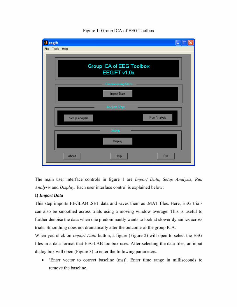
Figure 1: Group ICA of EEG Toolbox

The main user interface controls in figure 1 are Import Data, Setup Analysis, Run

Analysis and Display. Each user interface control is explained below:

I) Import Data

This step imports EEGLAB .SET data and saves them as .MAT files. Here, EEG trials

can also be smoothed across trials using a moving window average. This is useful to

further denoise the data when one predominantly wants to look at slower dynamics across

trials. Smoothing does not dramatically alter the outcome of the group ICA.

When you click on Import Data button, a figure (Figure 2) will open to select the EEG

files in a data format that EEGLAB toolbox uses. After selecting the data files, an input

dialog box will open (Figure 3) to enter the following parameters.

• ‘Enter vector to correct baseline (ms)’. Enter time range in milliseconds to

remove the baseline.

• ‘Do you want to smooth the EEG trials?’ Selecting ‘Yes’ means that the trials will

be smoothed using the selected moving window.

• ‘Enter a number for moving point average?’ Trials will be averaged using the

selected window length. For now leave it as 3.

• ‘How Do You Want To Sort Trials?’ You have the option to sort trials based on

condition and latency. For now leave it as ‘No’. Note that trial sorting makes

sense when (a) trial structure is different across subjects (b) sources are vastly

different between conditions and or behavioral outcomes. Sorting trials makes it

easier to identify components of interest in the display GUI, it does for the most

part not critically affect the accuracy of individual component reconstruction, for

illustration, in a typical oddball experiment, one can run the group ICA on

unsorted trials, and then sort the resulting components according to individual

RTs, which reconstructs the RT-dependency of later components that belong to

the P300 complex. EEGIFT can sort by RT and trial category, and employs the

EEG.event structure from EEGLAB for this.

• ‘Enter file name (not full path) for writing data.’ Data will be written in MAT file

format that EEGIFT uses for analyzing EEG data. The data will be saved in the

specified output directory (Figure 4) and the data set directory name will be the

same as the file name.

Figure 2: EEG File Selection

Figure 3: EEG Parameters

Figure 4: Output directory for saving the data

II) Setup ICA Setup ICA involves entering parameters for the group ICA analysis. The following are the

steps involved in this process:

a.) When you click on the Setup ICA button (Figure 1), a figure window (Figure 5) will

open to select the analysis output directory. All the output files will be stored in this

directory. After the directory is selected, a parameter select window will open. Figure 6

shows the initial parameter select window. Some of the user interface controls (Figure

10) are shielded from the user and plotted in "SetupICA-Defaults” menu. We explain the

main user interface controls followed by hidden user interface controls.

Figure 5: Analysis Output Directory

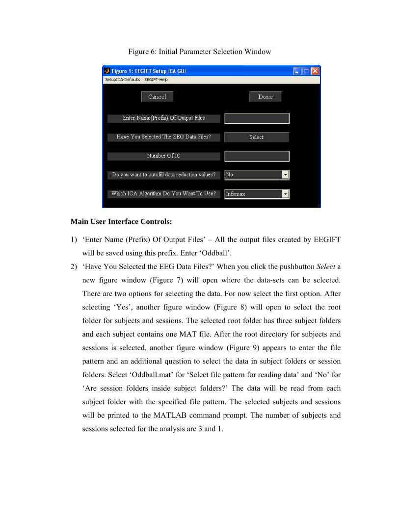
Figure 6: Initial Parameter Selection Window

Main User Interface Controls:

1) ‘Enter Name (Prefix) Of Output Files’ – All the output files created by EEGIFT

will be saved using this prefix. Enter ‘Oddball’.

2) ‘Have You Selected the EEG Data Files?’ When you click the pushbutton Select a

new figure window (Figure 7) will open where the data-sets can be selected.

There are two options for selecting the data. For now select the first option. After

selecting ‘Yes’, another figure window (Figure 8) will open to select the root

folder for subjects and sessions. The selected root folder has three subject folders

and each subject contains one MAT file. After the root directory for subjects and

sessions is selected, another figure window (Figure 9) appears to enter the file

pattern and an additional question to select the data in subject folders or session

folders. Select ‘Oddball.mat’ for ‘Select file pattern for reading data’ and ‘No’ for

‘Are session folders inside subject folders?’ The data will be read from each

subject folder with the specified file pattern. The selected subjects and sessions

will be printed to the MATLAB command prompt. The number of subjects and

sessions selected for the analysis are 3 and 1.

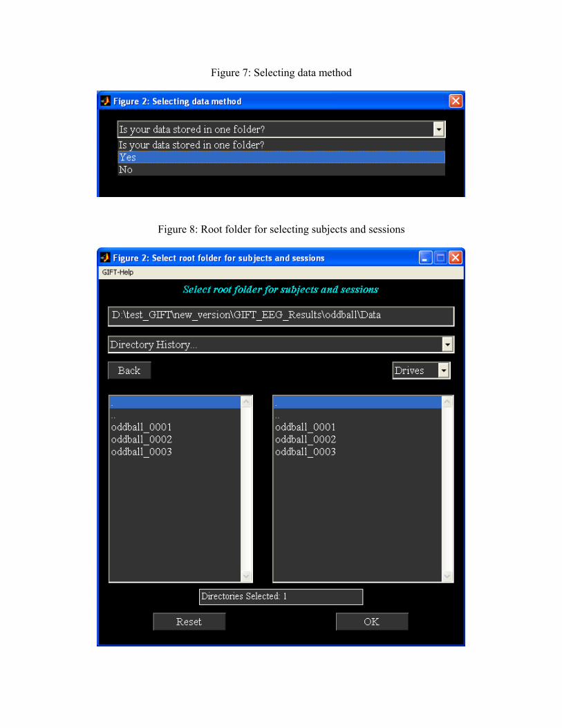
Figure 7: Selecting data method

Figure 8: Root folder for selecting subjects and sessions

Figure 9: File pattern and question for selecting data

Note: After the data is selected the pushbutton Select will be changed to popup

window with ‘Yes’ and ‘No’ as the options. ‘No’ option means the data files can

be selected again. ‘Yes’ option updates the data reduction parameters if the

parameter file is previously selected. The number of components will be auto

filled to 20 depending on the number of channels or electrodes.

3) ‘Number of IC’. Enter ‘20’. This refers to the number of independent

components extracted from the data.

4) ‘Do you want to auto fill data reduction values?’ By default this option is set

to ‘Yes’ when the data is selected and the ‘Number of IC’ is set to 20. For

now leave the options as ‘Yes’.

5) ‘Which ICA Algorithm Do You Want To Use?’ Select ‘Infomax’. Presently

there are 9 algorithms in the toolbox that can be used for EEG data like

Infomax, FastICA, Erica, Simbec, Evd, Jade Opac, Amuse, SDD ICA and

Radical ICA. A detailed explanation of algorithms like Infomax, FastICA,

Erica, Simbec, Evd and Jade Opac is given in the GIFT manual and in related

journal publications. By default, we employ Infomax since this algorithm has

been used most frequently in electrophysiology and neuroimaging to our

knowledge. The performance of the different algorithms is not remarkably

different when applied to aggregate EEG time domain data (See Appendix B).

Hidden User Interface Controls These user interface controls (Figure 10) will be shown after you click ‘Setup

ICA-Defaults’ menu (Figure 6). The parameters in Figure 10 are explained below:

1) ‘Do You Want To Scale The Results?’ The options available are ‘No’,

‘Calibrate’ and ‘Z-scores’.

a. 'Calibrate' – Components will be scaled to original data units by doing

a multiple regression using the time domain average of the component

as model and the average of the EEG signal from the original data as

observation. For each component, EEG signal from the original data is

computed by selecting the electrode that has the maximum absolute

value. For now select ‘Calibrate’.

b. 'Z-Scores' – Components will be converted to Z-scores.

2) 'How Many Reduction (PCA) Steps Do You Want To Run?' A maximum of

three reduction steps is provided. The number of reduction stages depends on

the number of data-sets (Table 1). For the example data-set two reduction

steps are automatically selected.

3) 'Number Of PC (Step 1)' - Number of principal components extracted from

each subject's session. For one subject one session this control will be disabled

as the number of principal components extracted from the data is the same as

the number of independent components.

4) 'Number Of PC (Step 2)' - Number of principal components extracted during

the second reduction step. This control will be disabled for two data reduction

steps as the number of principal components is the same as the number of

independent components.

5) 'Number Of PC (Step 3)' – This user interface control is disabled and set to 0

for the example data-set as there are only two data reduction steps. For data

sets with typical study sizes (e.g. 10-20 subjects), the number entered here

determines the number of independent components that are extracted. By

default, the number of principal components retained in the reduction steps

equals the number of independent components. This can be changed, e.g. from

a set of 20 principal components, one can extract e.g. 10 independent

components. While estimating lesser components can be reasonable in some

situations, extracting more independent components than principal

components is not recommend.

Figure 10: Hidden User Interface Controls

Table 1: Shows how groups are formed depending upon the number of data-sets

Number of Data-Sets (n)

Number of groups or reduction steps

n = 1 1 n < 4 2

4 <= n <= 10 User specified number (2 or 3) in “Setup ICA-Defaults” menu.

n > 10 3

b) Figure 11 shows the completed parameters window. Click Done button after selecting

all the answers for the parameters. This will open a figure window (Figure 12) to select

the ICA options. You can select the defaults, which are already selected in the dialog box

or you can change the parameters within the acceptable limits that are shown in the

prompt string. ICA options window can be turned off by changing defaults. Currently, the

dialog box is only available for the Infomax, FastICA, and SDD ICA. After selecting the

options, parameter file for the analysis is created in the working directory with the suffix

‘ica_parameter_info.mat’.

Figure 11: Completed Parameter Select Window

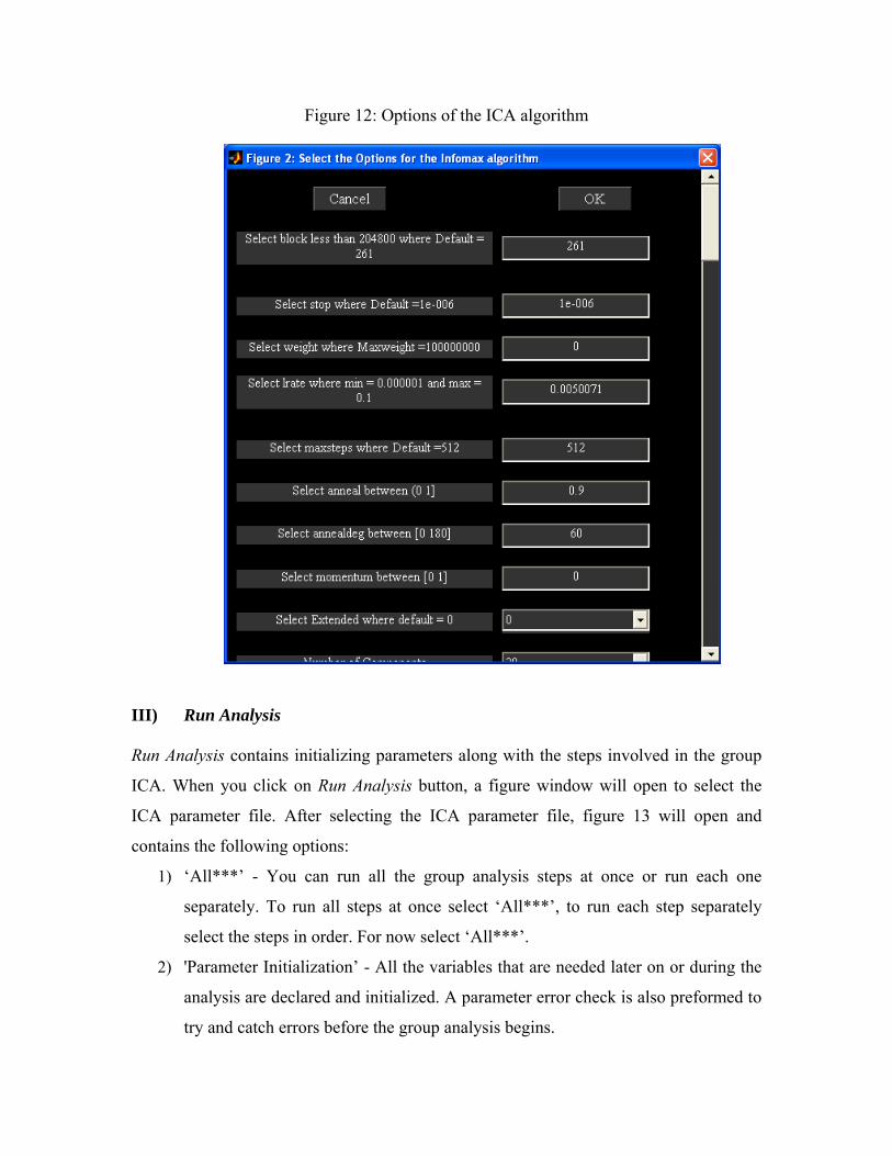
Figure 12: Options of the ICA algorithm

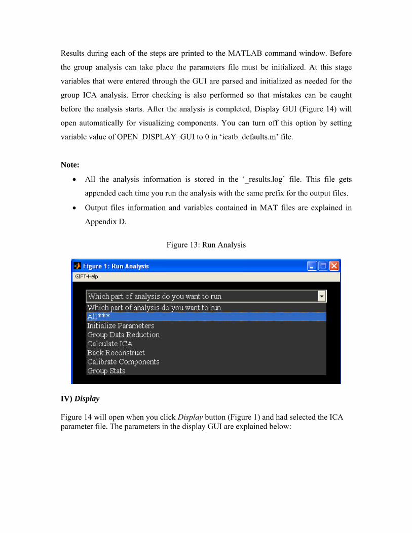
III) Run Analysis

Run Analysis contains initializing parameters along with the steps involved in the group

ICA. When you click on Run Analysis button, a figure window will open to select the

ICA parameter file. After selecting the ICA parameter file, figure 13 will open and

contains the following options:

1) ‘All***’ - You can run all the group analysis steps at once or run each one

separately. To run all steps at once select ‘All***’, to run each step separately

select the steps in order. For now select ‘All***’.

2) 'Parameter Initialization’ - All the variables that are needed later on or during the

analysis are declared and initialized. A parameter error check is also preformed to

try and catch errors before the group analysis begins.

3) 'Data Reduction' - Each data-set is reduced using Principal Components Analysis

(PCA). These reduced data-sets are then concatenated into a group or groups

depending on the number of data reductions steps selected, this process is

repeated. Each reduced data is saved in a MAT file and will be used in the back

reconstruction step. The second data reduction step demands most computing

resources (RAM) but works well for most current desktop/laptop PC

configurations and MATLAB versions. If an ‘out of memory error’ from

MATLAB occurs, try the usual steps to improve performance, e.g. clear the

workspace, terminate unused programs and background processes. If it still does

not work, reduce the number of principal components or change the input data

(e.g. lower sampling rate).

4) 'Calculate ICA' - The concatenated data from the data reduction step is used and

the aggregate ICA components are saved in MAT file format. Each component

consists of EEG time domain signal and weights.

5) 'Back Reconstruction' - The aggregate components and the results from data

reduction are used to compute the individual subject components. The individual

subject components are saved in MAT file format.

6) 'Calibrating Components' - The original EEG data is used to scale the

components from arbitrary units to data units or Z-scores.

7) 'Group Stats' - The individual back reconstructed components are used to compute

statistics on components like mean, standard deviation and t-test. Each component

consists of EEG time domain signal and topographic weights. For the t-test

weights of a session used is the same as the mean of weights of that session.

These group stats components are calculated for each session and are saved in

MAT file format.

Results during each of the steps are printed to the MATLAB command window. Before

the group analysis can take place the parameters file must be initialized. At this stage

variables that were entered through the GUI are parsed and initialized as needed for the

group ICA analysis. Error checking is also performed so that mistakes can be caught

before the analysis starts. After the analysis is completed, Display GUI (Figure 14) will

open automatically for visualizing components. You can turn off this option by setting

variable value of OPEN_DISPLAY_GUI to 0 in ‘icatb_defaults.m’ file.

Note:

• All the analysis information is stored in the ‘_results.log’ file. This file gets

appended each time you run the analysis with the same prefix for the output files.

• Output files information and variables contained in MAT files are explained in

Appendix D.

Figure 13: Run Analysis

IV) Display Figure 14 will open when you click Display button (Figure 1) and had selected the ICA parameter file. The parameters in the display GUI are explained below:

Figure 14: EEG Display GUI

1. ‘Select display method.’ There are two display methods like component and

subject. Each display method is explained below:

a. Component display method displays all components of a viewing set. You

can also select the components of interest in the component list box.

b. Subject display method displays a component of all viewing sets.

2. ‘Viewing Set’ – You can look at mean of all data sets, mean of one session,

individual data set components, etc.

3. ‘Component No:’ – Component numbers you want to look at. For subject display

method only one component can be selected whereas for component display

method more than one component can be selected.

4. “Display Defaults” menu - Display defaults are plotted in a figure which will

open when you click “Display Defaults” menu. The parameters in figure 15 are

explained below:

a. ‘Image Values’ – There are four options like ‘Positive and Negative’,

‘Positive’, ‘Absolute’ and ‘Negative’. For now select ‘Positive and

Negative’.

b. ‘Convert To Z-scores’ – You have the option to convert EEG signal of all

trials to Z-scores. For now select ‘Yes’. If you are looking at t-statistic

images, do not convert to Z-scores.

c. ‘Threshold Value’ – Z threshold applied on image. Select ‘1.0’.

d. ‘Components Per Figure’ – Options are ‘1’, ‘4’ and ‘9’. Select ‘4’.

Figure 15: Display Defaults

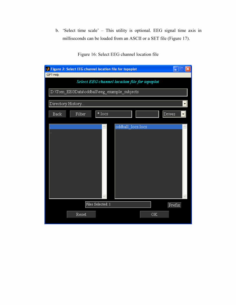
5. “Options” menu contains items like ‘Select EEG channel locs file’ and ‘Select

time scale’. Each item is explained below:

a. When you click ‘Select EEG channel locs file’, a figure (Figure 16) will

open to select the channel locations file for doing topography plots for

components. The default color map for topography plot is in

‘icatb_defaults.m’ file with the variable name

EEG_TOPOPLOT_COLORMAP.

b. ‘Select time scale’ – This utility is optional. EEG signal time axis in

milliseconds can be loaded from an ASCII or a SET file (Figure 17).

Figure 16: Select EEG channel location file

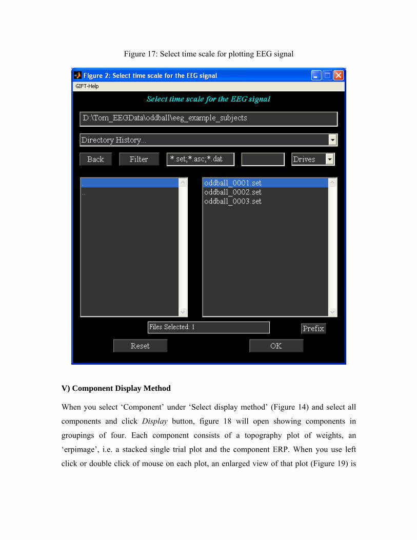
Figure 17: Select time scale for plotting EEG signal

V) Component Display Method When you select ‘Component’ under ‘Select display method’ (Figure 14) and select all

components and click Display button, figure 18 will open showing components in

groupings of four. Each component consists of a topography plot of weights, an

‘erpimage’, i.e. a stacked single trial plot and the component ERP. When you use left

click or double click of mouse on each plot, an enlarged view of that plot (Figure 19) is

shown in a new figure. You can browse around figures by using left arrow and right

arrow buttons at the end of the figure.

Figure 18: Components of mean of all data sets

Figure 19: Enlarged view of topography plot of component ‘001’

VI) Subject Display Method You have the option to view all data sets of a particular component when you select ‘Subject’ under ‘Select display method’ (Figure 14). Figure 20 shows individual subjects task related component results in groupings of four.

Figure 20: Task related component of 3 subjects

VII) Group ICA on 15 subjects We have done group ICA analysis on 15 subjects and extracted 20 components from the data. Figures 21 and 22 show task related component results using subject display method.

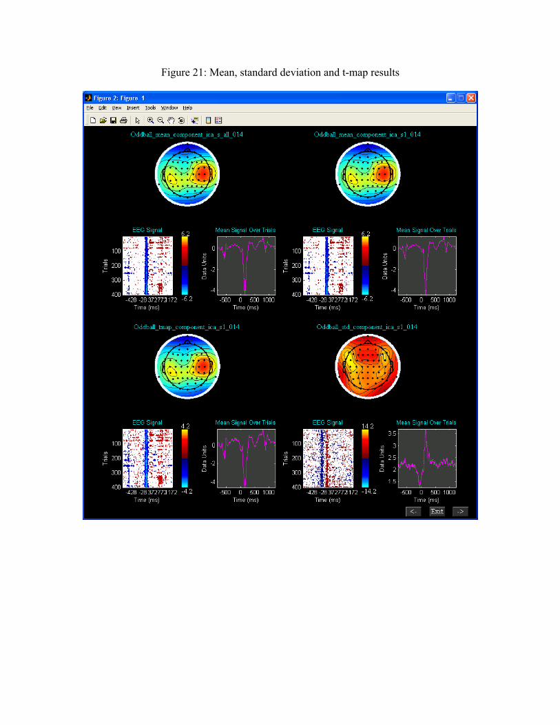
Figure 21: Mean, standard deviation and t-map results

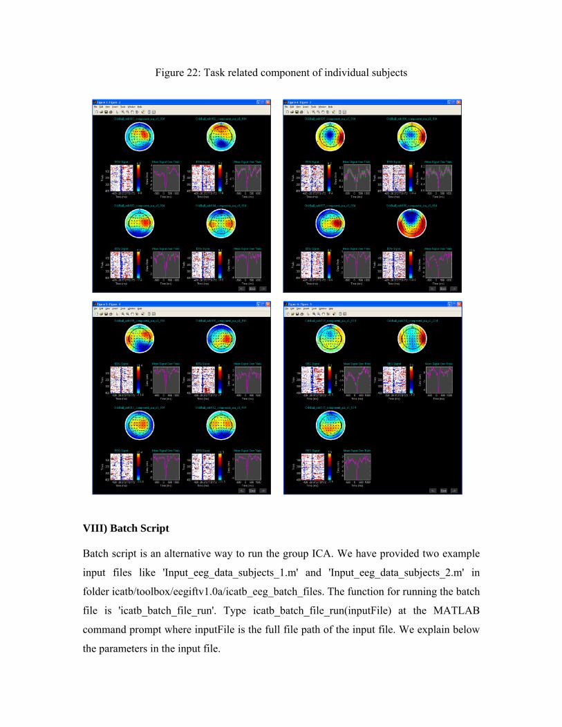
Figure 22: Task related component of individual subjects

VIII) Batch Script Batch script is an alternative way to run the group ICA. We have provided two example

input files like 'Input_eeg_data_subjects_1.m' and 'Input_eeg_data_subjects_2.m' in

folder icatb/toolbox/eegiftv1.0a/icatb_eeg_batch_files. The function for running the batch

file is 'icatb_batch_file_run'. Type icatb_batch_file_run(inputFile) at the MATLAB

command prompt where inputFile is the full file path of the input file. We explain below

the parameters in the input file.

• modalityType - Modality type. Enter 'EEG'.

• dataSelectionMethod - There are two ways to select the data. Options are 1 and 2.

Each option is explained below:

o 1 - Data will be selected automatically if you specify the root folder for

subjects and sessions, file pattern and a flag. Options for flag are

'data_in_subject_folder' and 'data_in_subject_subfolder'.

'data_in_subject_subfolder' - Data is selected from the subject sub-

folders. Number of sessions is equal to the number of sub-folders

containing the specified file pattern.

'data_in_subject_folder' - Data is selected from the subject folders.

The number of sessions is 1 and the number of subjects is equal to

the number of subject folders containing the specified file pattern.

o 2 - This option can be used when all the data is not in one directory. You

need to specify the data directory for each subject and session followed by

file pattern. The required variables are selectedSubjects and numOfSess.

selectedSubjects contains the arbitrary names of subjects (s1 refers to

subject1, s2 refers to subject 2, etc) and numOfSess contains the number

of sessions. Subject 1 session 1 data information must be entered in

variable s1_s1 and subject 2 session 2 information must be entered in

variable s1_s2.

• outputDir - Output directory of the analysis.

• prefix - All the output files will be pre-pended with this prefix.

• numReductionSteps - The number of reduction steps used and is dependent on the

number of data-sets used. A maximum of three reduction steps is used.

• numOfPC1 - Number of PC for reduction step 1.

• numOfPC2 - Number of PC for reduction step 2.

• numOfPC3 - Number of PC for reduction step 3.

• scaleType - Options are 0, 1 and 2. 0 means don't scale, 1 means scale

components to data units and 2 means scale components to Z-scores.

• algoType - Currently there are 9 ICA algorithms available in the EEGIFT

toolbox. The algorithms are as follows:

o 1 - Infomax

o 2 - FastICA

o 3 - ERICA

o 4 - SIMBEC

o 5 - EVD

o 6 - JADE OPAC

o 7 - AMUSE

o 8 - SDD ICA

o 9 - Radical ICA

Appendix A. Auditory Oddball Paradigm

The Auditory Oddball Paradigm (AOD) consisted of detecting an infrequent target sound within a

series of frequent regular sounds. The stimuli were presented via headphones, and participants

were asked to respond as quickly as possible by pushing a mouse button with their right index

finger. The standard stimulus was a center-panned 500 Hz tone, the target stimuli were left or

right-panned location deviants, respectively. Targets occurred with a probability of 0.20, 0.10 for

each location; the standard stimuli occurred with a probability of 0.80. Stimulus duration was 75

ms and the inter-stimulus interval was 700 ms, with no immediate repetitions of targets. In the

example data, the epochs contain a sequence of standard – target – standard sounds, to dissociate

between obligatory stimulus related and target related components, respectively. All stimuli were

presented at approximately 65 decibels above threshold. Response times ranged from 250-500

ms, the overall accuracy was larger than 98%.

Participants - 32 healthy right-handed undergraduates were recruited, and took part in the

experiment after providing a written statement of informed consent. Participants were sitting in a

comfortable recliner in an electro-magnetically shielded and sound-attenuated testing chamber

(Rainford EMC Systems, Wigan, UK). Participants were fitted with 63 Ag/AgCl scalp electrodes

mounted in an elastic cap (EasiCap, Falk Minow Services, Breitenbrunn, Germany) according to

the 10-20 System: FP1, FP2, F7, F3, Fz, F4, F8, T7, C3, Cz, C4, T8, P7, P3, Pz, P4, P8, O1, OZ,

O2, with additional intermediate sites at Fpz, AF7, AF3, AFz, AF4, AF8, FT7, FC5, FC3, FC1,

FCz, FC2, FC4, FC6, FT8, C5, C1, C2, C6, TP7, CP5, CP3, CP1, CPz, CP2, CP4, CP6, TP8, P5,

P1, P3, P6, PO7, PO3, POz, PO4, PO8, including mastoid sites TP9 and TP10. All channels were

referenced to the nose, with a ground electrode on the cheek, and impedances were kept below

10kΩ. Vertical eye movement (EOG) was acquired from a bipolar derivation between Fp1 and an

additional electrode placed below the left eye, horizontal EOG was acquired from a F7-F8 bipolar

montage. EEGs were recorded continuously at 500 Hz sampling frequency with a band-pass from

0.01-250 Hz with BrainAmp DC amplifiers (BrainProducts, Munich, Germany).

EEGs were down-sampled to 250 Hz, filtered with a zero-phase Butterworth filter from 1-45 Hz

(24 db per octave), and re-referenced to common average reference. The data were then

segmented from -800 to 1200 ms around target stimuli and baseline activity was defined from -

300 to 0 ms around stimulus onset, and trials with amplitudes exceeding ±150µV on any of the

channels were excluded from further analysis. Concatenated single sweeps around target onset,

including the previous and the following standards were subjected to single subject independent

component analysis (ICA, Infomax algorithm), implemented in EEGLAB (Delorme & Makeig,

2004) running in MATLAB. Components with topographies attributable to eye movement and

frontotemporal muscle activity were identified and removed from the data (Jung, et al., 2000). For

each dataset, we kept 20 components. Missing trials were padded with the mean from

surrounding trials. Hereafter, single-trials were additionally denoised with a wavelet filter (Quian

Quiroga & Garcia, 2003). Wavelet coefficients used for the reconstruction of the single trials

were selected on the basis of the grand-averaged response, and were the same for all electrode

sites and participants. Hereafter, group ICA was computed, estimating 20 PC/ICs.

B. Hybrid Results

Unlike the general linear model, ICA is not naturally suited to generalize results from a group of

subjects. The solution that we selected here is to create aggregate data containing observations

from all subjects, estimate a single set of components and then back-reconstruct these in the

individual data. For estimation of the group temporal ICA we employ the rationale proposed by

Calhoun (Calhoun, Adali, Pearlson, & Pekar, 2001), where the concatenation of multiple datasets

into one matrix is instantiated via two data reduction steps prior to estimation of independent

components. PCA is used for dimensionality reduction on the single trial data from all EEG

channels in each participant, and subsequently on aggregated data. Hereafter ICA is performed,

estimating a single set of components, thus identifying and ordering the same components in

different subjects in the same way. The component time courses for individual subjects are back-

reconstructed from the aggregate mixing matrix by multiplying the partition of W corresponding

to the respective subject with the corresponding partition of the data. The individual un-mixing

matrices are separable across subjects and the back-reconstructed data is a function of primarily

the data within subjects (See figure 24). When used for EEG time series analysis, the accuracy of

component detection and back-reconstruction with this group model is dependent on the degree

of intra and inter individual time and phase-locking of event related EEG processes. We illustrate

this dependency here by generating hybrid data for 20 datasets that consist of three simulated

event-related sources with varying degrees of latency jitter and variable topographies (S1-S3, see

figure 24, As top left and to right for examples of two individual datasets), mixed with real EEG

data (See figure 24, x middle), and compute the group ICA solution (See figure 24, Wy bottom).

Reconstruction accuracy, expressed as the variance of the source accounted for by the

reconstructed IC averaged across the 20 datasets (R2) was tested for latency jitter 1, 2 and 3 times

the FWHM of the source ERPs for a number of algorithms (Table 2). The results show that

group ICA is adequate for decomposition of single trial ERPs with physiological jitter, and will

reconstruct such sources with approx. 70-90% accuracy both temporally, and spatially.

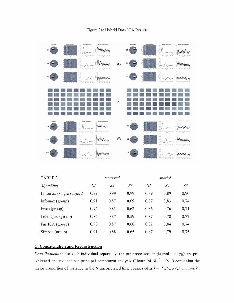
Figure 24: Hybrid Data ICA Results

TABLE 2 temporal spatial

Algorithm S1 S2 S3 S1 S2 S3

Iinfomax (single subject) 0,99 0,99 0,99 0,89 0,89 0,90

Infomax (group) 0,91 0,87 0,69 0,87 0,83 0,74

Erica (group) 0,92 0,85 0,62 0,86 0,76 0,71

Jade Opac (group) 0,85 0,87 0,59 0,87 0,78 0,77

FastICA (group) 0,90 0,87 0,68 0,87 0,84 0,74

Simbec (group) 0,91 0,88 0,65 0,87 0,79 0,75 C. Concatenation and Reconstruction

Data Reduction: For each individual separately, the pre-processed single trial data y(j) are pre-

whitened and reduced via principal component analysis (Figure 24, R1-1… RM

-1) containing the

major proportion of variance in the N uncorrelated time courses of x(j) = [x1(j), x2(j), …, xN(j)]T.

PCA whitening preconditions the data and simplifies ICA estimation due to the orthogonal

projection, reduction of complexity, and de-noising, as well as compressing the data and thus

reducing the computational load. Group data is generated by concatenating individual principal

components in the aggregate data set G. In detail, let Xi = Ri-1Yi be the L-by-V reduced data matrix

from subject i where Yi is the K-by-V data matrix containing preprocessed EEG epochs from all

channels, Ri-1 is the L-by-K reducing matrix from the principal component decomposition, V is the

number of time points (samples per epoch * trials), K is the number of scalp channels, and L is

the size of the channel dimension following reduction. The next step is to concatenate the reduced

data from all subjects into a matrix and reduce this matrix to N, the number of components to be

estimated. The N-by-V reduced, concatenated matrix for the M subjects is

(1)

Where G-1 is an N-by-LM reducing matrix from a second PCA decomposition and is multiplied on

the right by the LM-by-V concatenated data matrix for the M subjects.

ICA Estimation: After concatenation of individual principal components in the aggregate data set

G, this matrix is decomposed by ICA, estimating the optimal inverse of the mixing matrix Â, and

a single set of source time courses (ŝ). Following ICA estimation, we can write X = ÂŜ, where Â

is the N-by-N mixing matrix and Ŝ are the N-by-V component time courses. Substituting this

expression for X into equation (1) and multiplying both sides by G results in

(2)

Partitioning and single subject reconstruction: Partitioning the matrix G by subject provides the

following expression

(3)

We then write the equation for subject i by working only with the elements in partition i of the

above matrices such that

(4)

The matrix Ŝi in equation 4 contains the single subject component timecourses for subject i,

calculated from the following equation

(5)

We now multiply both sides of equation 4 by Ri and write

(6)

yielding the ICA decomposition of the data from subject i contained in the matrix Yi. The N-by-V

matrix Ŝi contains the N component time courses, and the K-by-N matrix is the single

subject mixing matrix, yielding the scalp maps for N components.

D. Output Files

1. Subject File – Subject file contains information about number of subjects, sessions and input

files. It is saved with suffix ‘Subject.mat’. The following are the variables in the MAT file:

• numOfSub – Number of subjects.

• numOfSess – Number of sessions.

• files – Input files stored in a data structure.

2. Parameter File – Parameter file contains user input and analysis output files information. It is

stored with suffix ‘_ica_parameter_info.mat’. The MAT file contains sesInfo data structure and

the user input information is stored in sesInfo.userInput.

3. Data reduction (PCA) - After PCA step, the data reduction information is stored in a MAT file

with suffix ‘_pca_ra-b.mat’ where a refers to reduction step number and b refers to data-set

number. The following are the variables in the PCA file:

• V – Eigen vectors whose dimensions are electrodes by components.

• Lambda – Eigen values diagonal matrix of dimensions components by components.

• pcasig – Reduced data of dimensions time*trials by components.

• whiteM – Whitening matrix of dimensions components by electrodes.

• dewhiteM – Pseudo inverse of whitening matrix of dimensions electrodes by

components. This will be used while reconstructing individual subject components during

the back reconstruction step.

4. ICA - After ICA step, the aggregate components information is stored in a MAT file with the

suffix ‘_ica.mat’. The following are the variables in the ICA file:

• W – Un-mixing matrix of dimensions components by components.

• A – Pseudo inverse of W and is of dimensions components by components.

• icasig – Independent source signals of dimensions components by time*trials.

5. Back reconstruction – Back reconstruction files are saved with suffix ‘_brn.mat where n refers

to the data-set number. The MAT file contains compSet data structure with the following fields:

• timecourse - EEG signal of dimensions components by time*trials.

• Topography - Weights matrix of dimensions electrodes by components.

6. Calibrate – Calibrate step files are saved with suffix ‘*ca-b.mat’ where a refers to subject

number and b refers to session number. The following variables are in the calibrate step file:

• timecourse - Scaled EEG signal of dimensions components by time*trials.

• topography - Scaled weights matrix of dimensions electrodes by components.

7. Group stats – Group stats files are saved with suffix ‘_component_ica_’ in MAT format. Each

MAT file contains time courses (EEG signal) and topography (weights matrix) of the same

dimensions as in the calibrate step file.

E. Defaults

EEG defaults are in ‘icatb_defaults.m’ file. In GIFT manual and walk-through we explained

necessary variables required for analysis and display. We explain below EEG specific variables

used in EEGIFT:

• EEG_RMBASE – Vector used for removing baseline from EEG signal during smoothing

trials. The default value is [-100 0].

• EEG_IMAGE_VALUES – Image values used for displaying stacked EEG signal. The

options available are ‘Positive and Negative’, ‘Positive’, ‘Absolute’ and ‘Negative’. The

default value is ‘Positive and Negative’.

• EEG_CONVERT_Z – Option is provided to convert stacked EEG image to Z-scores

during display. The default value is ‘Yes’.

• EEG_THRESHOLD_VALUE – Threshold used for displaying stacked EEG signal. The

default value is ‘1.0’.

• EEG_IMAGES_PER_FIGURE - The number of components per figure that can be

displayed. The options available are ‘1’, ‘4’ and ‘9’. The default value is ‘4’.

• EEG_TOPOPLOT_COLORMAP – Color map used for topography plot. The default

value is ‘jet(64)’.

References

Calhoun, V.D., Adali, T., Pearlson, G.D., & Pekar, J.J. (2001). A method for making group

inferences from functional MRI data using independent component analysis. Hum Brain

Mapp, 14(3), 140-51.

Delorme, A., & Makeig, S. (2004). EEGLAB: an open source toolbox for analysis of single-trial

EEG dynamics including independent component analysis. J Neurosci Methods, 134(1),

9-21.

Eichele, T., Calhoun, V.D., Moosmann, M., Specht, K., Jongsma, M.L., Quiroga, R.Q., Nordby,

H., & Hugdahl, K. (2008). Unmixing concurrent EEG-fMRI with parallel independent

component analysis. Int J Psychophysiol, 67(3), 222-34.

Jung, T.P., Makeig, S., Humphries, C., Lee, T.W., McKeown, M.J., Iragui, V., & Sejnowski, T.J.

(2000). Removing electroencephalographic artifacts by blind source separation.

Psychophysiology, 37(2), 163-78.

Quian Quiroga, R., & Garcia, H. (2003). Single-trial event-related potentials with wavelet

denoising. Clin Neurophysiol, 114(2), 376-90.