1

Group Factor AnalysisArto Klami, Seppo Virtanen, Eemeli Leppaaho, and Samuel Kaski

F

Abstract—Factor analysis provides linear factors that describe relation-ships between individual variables of a data set. We extend this clas-sical formulation into linear factors that describe relationships betweengroups of variables, where each group represents either a set of relatedvariables or a data set. The model also naturally extends canonical cor-relation analysis to more than two sets, in a way that is more flexible thanprevious extensions. Our solution is formulated as variational inferenceof a latent variable model with structural sparsity, and it consists of twohierarchical levels: The higher level models the relationships betweenthe groups, whereas the lower models the observed variables given thehigher level. We show that the resulting solution solves the group factoranalysis problem accurately, outperforming alternative factor analysisbased solutions as well as more straightforward implementations ofgroup factor analysis. The method is demonstrated on two life sciencedata sets, one on brain activation and the other on systems biology,illustrating its applicability to the analysis of different types of high-dimensional data sources.

Index Terms—factor analysis, multi-view learning, probabilistic algo-rithms, structured sparsity

1 INTRODUCTION

Factor analysis (FA) is one of the cornerstones of dataanalysis, the tool of choice for capturing and understand-ing linear relationships between variables [1]. It providesa set of K factors, each explaining dependencies betweensome of the features in a vectorial data sample yi ∈ RDbased on the model

yi =K∑k=1

zi,kwk + εi,

where zi,k is the value of the kth unobserved factor,wk ∈ RD contains its loadings, and εi is Gaussian noise.To correctly capture the relationships, we need to assumea diagonal noise covariance with free variance for eachof the variables. If the noise model was more flexible,having non-diagonal covariance, it would allow describ-ing some of the relationships as noise. On the otherhand, forcing the variances to be equal would implythat heteroscedastic noise would need to be explainedas factors, reducing the model to probabilistic PCA [2].

• A. Klami and S. Kaski are with Helsinki Institute for Information Tech-nology HIIT, Department of Computer Science, University of Helsinki.E-mail: arto.klami@hiit.fi, samuel.kaski@hiit.fi

• S. Virtanen, E. Leppaaho and S. Kaski are with Helsinki Institute forInformation Technology HIIT, Department of Information and ComputerScience, Aalto University.E-mail: seppo.j.virtanen@aalto.fi,eemeli.leppaaho@aalto.fi

Building on our preliminary conference paper [3], wegeneralize factor analysis to a novel problem formula-tion of group factor analysis (GFA), where the task is toexplain relationships between groups of variables. Weretain the linear-Gaussian family of FA, but modify themodel so that each factor now describes dependenciesbetween some of the feature groups instead of individualvariables. Again the choice of residual noise is crucial: itneeds to be flexible enough to model everything that isnot a true relationship between two variable groups, butrestricted enough so that all actual relationships will bemodeled as individual factors. For FA these requirementswere easily satisfied by assuming independent variancefor each dimension. For GFA more elaborate construc-tions are needed, but the same basic idea applies.

From another perspective, GFA extends multi-batteryfactor analysis (MBFA), introduced by McDonald [4]and Browne [5] as a generalization of inter-battery fac-tor analysis (IBFA) [6], [7] to more than two variablegroups. MBFA is a factor analysis model for multipleco-occurring data sets, or, equivalently, for a vectorialdata sample whose variables have been split into groups.It includes a set of factors that model the relationshipsbetween all variables, as well as separate sets of factorsexplaining away the noise in each of the variable groups.These group-specific factor sets are sufficiently flexiblefor modeling all variation within each group. However,each of the remaining factors is assumed to describerelationships between all of the groups, which is not suf-ficient for providing interpretable factors that reveal therelationships between the data sets as will be explainedbelow. Nevertheless, the MBFA models are useful toolsfor multi-source data analysis, illustrated by the fact thatthe problem has been re-discovered in machine learningliterature several times; see Section 4 for more details.

To solve the GFA problem, we need to have alsofactors that describe relationships between subsets ofthe groups. This makes the solutions to the problemboth more flexible and more interpretable than MBFA.For example, a strong factor tying two groups whilebeing independent of the other groups can then beexplicitly modeled as such. The MBFA-based modelswould, falsely, reveal such a factor as one that is sharedby all groups. Alternatively, they would need to, againincorrectly, split them into multiple group-specific ones.

In recent years, the need for the GFA solution hasbeen identified by several authors, under different ter-

arX

iv:1

411.

5799

v2 [

stat

.ML

] 2

Dec

201

4

2

minology. Jia et al. learned sparse matrix factorization byconvex optimization [8], and Van Deun et al. used group-lasso penalty to constrain the factors of a simultaneouscomponent analysis (SCA) model [9]. Various Bayesiantechniques have also been proposed for learning sharedand individual subspaces of multiple data sources [3],[10], [11], [12].

In this work we lay the foundation for future develop-ment of GFA solutions, by properly defining the prob-lem setup and terminology. We also present a generalsolution outline and show that the solutions mentionedabove are all instances of the same basic approach; theyall learn structured sparse FA models with varying tech-niques for obtaining group-wise sparsity for the factorloadings. We then propose a novel GFA solution thatdoes not make a strong simplifying assumption sharedby all the previous approaches. They all assume thatwe can independently infer, for each factor-group pair,whether that factor describes variation related to thatgroup, whereas our solution explicitly models also theseassociations with an additional linear model. In brief, ourmodel hence consists of two linear hierarchical levels.The first models the relationships between the groups,and the latter models the observed data given the outputof the higher level. Alternatively, it can be viewed asa direct generalization of [3] with a more advancedstructured sparsity prior making it possible to reducethe degrees of freedom in the model when needed.

Before delving into the details on how we solve theGFA problem, we introduce some general applicationscenarios. The model is useful for analyzing multi-view setups where we have several data sets with co-occurring samples. The variables can be grouped accord-ing to the data sets: all variables in one set belong to onegroup etc. Then GFA explains relationships between datasources, and for two data sets it equals the problem ofcanonical correlation analysis (CCA; see [13] for a recentoverview from a probabilistic perspective). Alternatively,each group could contain a collection of variables chosento represent a multi-dimensional concept, such as cogni-tive abilities of a subject, which cannot be summarizedwith a single feature. Then GFA could be used for asso-ciating cognitive abilities with other multi-dimensionalconcepts. The groups can also represent a meaningfulpartitioning of larger data sets; we present two practicalexamples of this kind of a setup. In one example wesplit a high-dimensional feature vector over the humangenome into subsets according to functional pathwaysto describe drug responses, and in the other examplewe split magnetic resonance images of the human braininto local regions to study relationships between brainareas.

2 GROUP FACTOR ANALYSIS

2.1 Problem formulationThe group factor analysis problem is as follows: Assumea collection of observations yi ∈ RD for i = 1, . . . , N

collected in a data matrix Y ∈ RN×D, and a disjointpartition of the D variables into M groups {Gm}. TheGFA task is to find a set of K factors that describe Y sothat relationships between the groups can be separatedfrom relationships within the groups. For notationalsimplicity, assume that the first D1 variables correspondto the first group G1, the following D2 variables to G2,and so on. Then we can write Y = [X(1), ...,X(M)], whereX(m) is a subset of the data corresponding to Gm. We usex(m)i to denote the ith sample (row) of X(m). Throughout

this paper we use the superscript (m) to denote variablesrelated to the mth group or data set.

2.2 General solution

A general solution to the GFA problem can be formu-lated as a joint factor model for the observed data sets.The model for the mth group of the ith sample is

x(m)i ∼ N (W(m)>zi, τ

−1m I), (1)

where W(m)> = [w(m)1 , . . . ,w

(m)K ], zi ∈ RK , and τm

is noise precision. Equivalently, we can directly writeyi = W>zi+εi, where εi is Gaussian noise with diagonalcovariance but separate variance for each group, bydenoting W = [W(1), ...,W(M)].

To make the factors interpretable in the GFA-sense,that is, to describe relationships between the groups, weneed to make W sparse so that it satisfies the followingproperties (for a visual illustration see Figure 1):

1) Some factors are private to each group, so thatw

(m)k 6= 0 only for one m. These factors explain

away the variation independent of all the othergroups, and play the role of residual noise inregular FA.

2) The rest of the factors describe relationships be-tween some arbitrary subset of the groups; they arenon-zero for those groups and zero for the others.

A trivial solution would explicitly split the factors intoseparate sets so that there would be one set of factorsfor each possible subset of the groups (including thesingletons and the set of all groups). This can be done forsmall M ; for example Klami and Kaski proposed sucha model for M = 2 [14] and Gupta et al. formulatedthe model for general M but ran experiments only withM = 3 [10]. Due to the exponential number of subsets,these approaches cannot generalize to large M .

A better approach is to associate the projection matrixW with a structural sparsity prior that encourages solu-tions that satisfy the necessary properties. This strategywas first presented for M = 2 by Virtanen et al. [15],and extended for general M independently by severalauthors [3], [11], [12]. Despite technical differences inhow the structural sparsity is obtained, all of theseapproaches can be seen as special instances of our GFAsolution principle. Also the non-Bayesian models thatcan be used to solve the GFA problem follow the sameprinciple [8], [9].

3

Sam

ples

Group 1 Group 2 Group 3

≈

LatentFactor loadings

Active in all groupsActive in a subset of groups“Noise” factors

X(1) X(2) X(3) Z

W

variables

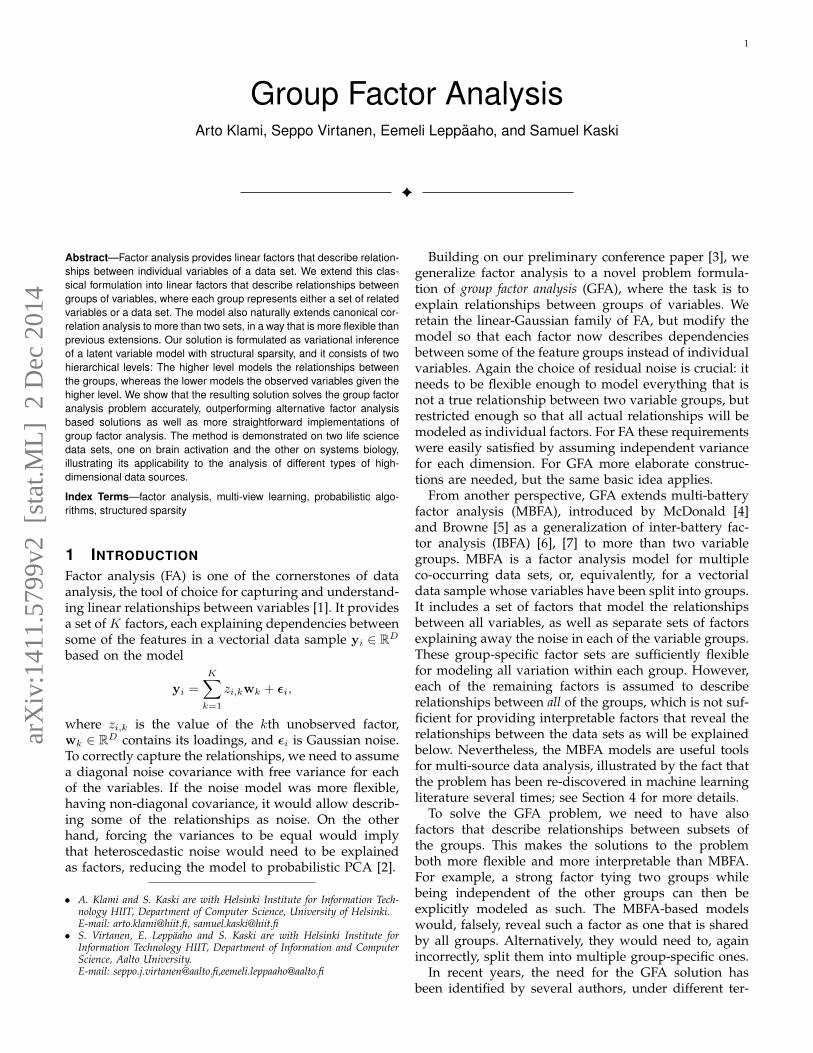
Fig. 1. Illustration of the group factor setup for three groups. The model learns a linear factorization of a data matrixY = [X(1),X(2),X(3)] whose features have been split into (here) three groups, so that the factor loadings W aregroup-wise sparse. The model then automatically learns which factors describe dependencies between either all ofthe groups or a subset of them, and which describe structured noise specific to each group. The sparsity structure ofW is here represented by coloring; the white areas correspond to zeros whereas the gray areas are non-zero.

3 MODEL

We propose a novel GFA solution that is another instanti-ation of the general approach described above. The tech-nical novelty is in a more advanced structural sparsityprior which takes into account possible dependenciesbetween the groups, instead of assuming the group-factor activations to be a priori independent as in theearlier solutions. The model can also be interpreted as atwo-level model that uses one level to model associationstrengths between individual groups and the other levelto model the observations given the association strength.This interpretation clarifies the conceptual novelty, ex-plicating how the new structural sparsity prior has anintuitive interpretation.

The generative model is the one given in (1) coupledwith suitable priors. For zi we use the unit Gaussianprior zi ∼ N (0, I), and for the noise precisions τm weemploy a gamma prior with both shape and rate param-eters set to 10−14; the model is fairly insensitive to thesehyperparameters. To find a GFA solution these standardchoices need to be complemented with structured sparsepriors for W, described next.

3.1 Sparsity prior

We denote by αm,k the inverse strength of associationbetween the mth group and the kth factor, and directlyinterpret it as the precision parameter of the prior distri-bution for w

(m)k , the projection mapping the kth factor

to the observed variables in the mth group. That is, weassume the prior

p(W|α) =

M∏m=1

K∏k=1

Dm∏d=1

N (w(m)k,d |0, α

−1m,k).

The same prior was used in our preliminary work [3],where we drew αm,k independently from a flat gammaprior to implement group-wise extension to automaticrelevance determination (ARD).

Here we replace the independent draws with a linearmodel for α to explicitly model the association strengthsbetween group-factor pairs. Since the entries correspond

U

V

τ x(m)i W(m)

zi

m = 1...Mi = 1...N

αm

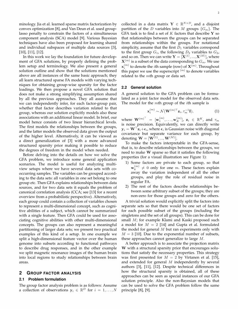
Fig. 2. Plate diagram of group factor analysis. The ob-servation model, used also by earlier GFA solutions, ishighlighted by the blue dotted region, whereas the novellow-rank model for the group-factor associations is indi-cated by the orange dashed region.

to precisions for the second level projections, we modelthem in the log-space as

logα = UV> + µu1> + 1µ>v , (2)

where U ∈ RM×R and V ∈ RK×R. The vectors µu ∈ RMand µv ∈ RK model the mean profiles. Here R is therank of the linear model, and typically R � min(M,K)so that we get a low-rank decomposition for the associa-tion strengths, obtained by element-wise exponentiationα = exp(UV> + µu1

> + 1µ>v ). Finally, we place anelement-wise normal prior for the matrices U and Vwith zero mean and precision set to a fixed constantλ = 0.1; extensions to further hierarchical priors wouldalso be tractable if needed. The resulting GFA model isvisualized as a plate diagram in Figure 2, highlightingthe two levels of the model.

The motivation for modeling the αm,k instead ofassuming them independent comes from the originalmodeling task of GFA. The goal is to understand therelationships between the groups, and hence we shouldexplicitly model them. The earlier models with inde-pendent priors assume that the groups are independent,which is unlikely to hold in practical applications. Ourmodel, in turn, directly represents correlations betweenthe group activation profiles.

An alternative formulation for correlated groupswould directly draw logαm from a multivariate distri-

4

bution, such as multivariate normal [16]. However, spec-ifying the correlations for such a model would requireM(M−1)/2 parameters, making the approach infeasiblefor large M . Since modeling the correlations is expectedto be the most useful for large number of groups, it isclearly beneficial to use the low-rank model that requiresonly (M +K)× (R+ 1) parameters.

3.2 InterpretationAs mentioned above, the model can be interpreted intwo alternative ways. The straightforward interpretationis that of a factor analysis model for the D observedvariables, with a structural sparsity prior for makingthe projections implement the GFA properties. Thisviewpoint illustrates the relationship between the earlierBayesian solutions for GFA [3], [11], [12]; they follow thesame general approach presented in Section 2.2, but oursparsity prior is more advanced.

Perhaps the more interesting interpretation is to con-sider (2) as the primary model. Then the entries of α areconsidered as unobserved data describing the groups;U are the factor loadings and V provide the latentfactors for the groups. The mapping from α to theobservations, parameterized by Z and W, is then merelya set of nuisance parameters. From this perspective,the earlier models presented for the GFA problem arevery simple. They do not assume any structure betweenthe groups, but instead draw the association strengthsindependently. Their results will naturally still revealsuch associations, but not as well as the proposed modelthat models them explicitly.

As we later empirically demonstrate, the rank R of thegroup association level can typically be very low evenfor very high-dimensional data collections with a largenumber of groups. This makes it possible to visuallystudy the associations between the groups, for examplevia a scatter plot of the columns of U for R = 2. Wediscuss approaches for determining the value of R forpractical applications in Section 5.4.

3.3 InferenceFor inference, we use mean-field variational approxi-mation. We approximate the posterior with a factorizeddistribution

q(Θ) = q(Z)q(W)q(τ )q(U)q(V),

where Θ = {Z,W, τ ,U,V}, and find the approximationthat minimizes the Kullback-Leibler divergence fromq(Θ) to p(Θ|Y). Equivalently, this corresponds to es-timating the marginal likelihood p(Y) with maximallower bound,

log p(Y) ≥ L(Θ) =

∫q(Θ) log

p(Θ,Y)

q(Θ).

The mean-field algorithm proceeds by updating each ofthe terms in turn, always finding the parameters thatmaximize the expected lower bound L(Θ), given all the

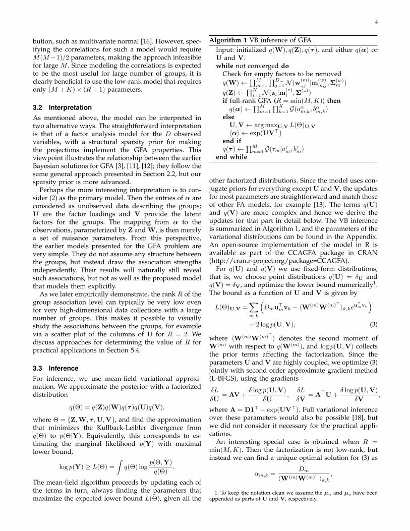
Algorithm 1 VB inference of GFAInput: initialized q(W), q(Z), q(τ ), and either q(α) orU and V.while not converged do

Check for empty factors to be removedq(W)←

∏Mm=1

∏Dm

j=1N (w(m):,j |m

(w)m,j ,Σ

(w)m )

q(Z)←∏Ni=1N (zi|m(z)

i ,Σ(z))if full-rank GFA (R = min(M,K)) thenq(α)←

∏Mm=1

∏Kk=1 G(aαm,k, b

αm,k)

elseU,V← arg maxU,V L(Θ)U,V〈α〉 ← exp(UV>)

end ifq(τ )←

∏Mm=1 G(τm|aτm, bτm)

end while

other factorized distributions. Since the model uses con-jugate priors for everything except U and V, the updatesfor most parameters are straightforward and match thoseof other FA models, for example [13]. The terms q(U)and q(V) are more complex and hence we derive theupdates for that part in detail below. The VB inferenceis summarized in Algorithm 1, and the parameters of thevariational distributions can be found in the Appendix.An open-source implementation of the model in R isavailable as part of the CCAGFA package in CRAN(http://cran.r-project.org/package=CCAGFA).

For q(U) and q(V) we use fixed-form distributions,that is, we choose point distributions q(U) = δU andq(V) = δV, and optimize the lower bound numerically1.The bound as a function of U and V is given by

L(Θ)U,V =∑m,k

(Dmu>mvk − 〈W(m)W(m)>〉k,keu

>mvk

)+ 2 log p(U,V), (3)

where 〈W(m)W(m)>〉 denotes the second moment ofW(m) with respect to q(W(m)), and log p(U,V) collectsthe prior terms affecting the factorization. Since theparameters U and V are highly coupled, we optimize (3)jointly with second order approximate gradient method(L-BFGS), using the gradients

δL

δU= AV +

δ log p(U,V)

δU,

δL

δV= A>U +

δ log p(U,V)

δV,

where A = D1> − exp(UV>). Full variational inferenceover these parameters would also be possible [18], butwe did not consider it necessary for the practical appli-cations.

An interesting special case is obtained when R =min(M,K). Then the factorization is not low-rank, butinstead we can find a unique optimal solution for (3) as

αm,k =Dm

〈W(m)W(m)>〉k,k,

1. To keep the notation clean we assume the µu and µv have beenappended as parts of U and V, respectively.

5

assuming λ is negligibly small. This is identical to thevariational update for a model that draws αm,k from agamma prior with the parameters approaching zero (theuniform distribution limit of gamma). This is the priorused by some of the earlier GFA solutions [3], [12], andhence we get the earlier models as special cases of ours.

The inference scales linearly in M , D and N , andhas cubic complexity with respect to K. In practice,it is easily applicable for large data sets as long asK is reasonable (at most hundreds). However, duringinference empty factors may occur and in this case theycan be removed from the model to speed up and stabilizecomputation2.

3.4 Predictive inferenceEven though the GFA model is in this work formulatedprimarily as a tool for exploring relationships betweenvariable groups, it can readily be used also as a predic-tive model. In this prediction setting new (test) samplesare observed for a subset of groups and the task is topredict unobserved groups based on observed data.

For simplicity of presentation, we assume that only themth group is unobserved. Then the missing data are rep-resented by the predictive distribution p(X(m)∗ |Y−(m)∗),where Y−(m)∗ denotes partially observed test data con-sisting of all the other groups. However, this distri-bution involves marginalization over both W and Zthat is analytically intractable and hence we need toapproximate it. In particular, given Y−(m)∗ , q(W) andq(τ ), we learn the approximate posterior distribution forthe latent variables q(Z∗) corresponding to Y−(m)∗ andapproximate the mean of the predictive distribution as

〈X(m)∗ |Y−(m)∗〉 = 〈Z∗W(m)〉q(W(m)),q(Z∗)

= Y−(m)∗T〈W−(m)>〉Σ−1〈W(m)〉, (4)

where T = diag({〈τj〉IDj}j 6=m) and Σ = IK +∑j 6=m〈τj〉〈W(j)W(j)>〉. In the experiments we use this

mean value for prediction.

4 RELATED WORK

The GFA problem and our solution for it are closelyrelated to several matrix factorization and factor anal-ysis techniques. In the following, the related work isdiscussed from two perspectives. First we cover othertechniques for solving the group factor analysis problemor its special cases. Then we proceed to relate the pro-posed solution to multiple regression, which is a specificuse-case for GFA.

4.1 Factor models for multiple groupsFor a single group, M = 1, the model is equivalentto Bayesian principal component analysis [2], [17]; allof the factors are active for the one group and they

2. We remove the kth factor from the model if ck =∑Ni=1〈zi,k〉2/N < 10−7.

describe the variation with linear components. We canalso implement sparse FA with the model, by settingM = D so that each group has only one variable.The residual noise has independent variance for eachvariable, and the projections become sparse because ofthe ARD prior.

For two groups, M = 2, the model is equivalentto Bayesian CCA and inter-battery factor analysis [13];some factors model the correlations whereas some de-scribe the residual noise within either group.

Most multi-set extensions of CCA, however, are notequivalent to our model. For example, Archambeau etal. [19] and Deleus et al. [20] extend CCA for M > 2,but instead of GFA they solve the more limited problemof multiple-battery factor analysis [4], [5]. The MBFAmodels provide one set of factors that describe the rela-tionships between all groups, and then model the varia-tion specific to each group either with a free covariancematrix or a separate set of factors for that group. Besidesthe multi-set extensions of CCA, also the probabilisticinterpretation of sparse matrix factorization [21], andthe JIVE model for integrated analysis of multiple datatypes [22], [23] belong to the family of MBFA models.These models differ in their priors, parameterization andinference, but are all conceptually equivalent.

In recent years, a number of authors have indepen-dently proposed solutions for the GFA problem. Theyall follow the general solution outline presented in Sec-tion 2.2 with varying techniques for obtaining the group-wise sparsity. Common to all of them is that they do notexplicitly model the relationships between the groups,but instead assume that the choice of whether a factordescribes variation in one particular group can be madeindependently for all factor-group pairs. This holds forthe non-Bayesian solutions of multi-view sparse matrixfactorizations [8] and the group lasso penalty variantof SCA [9], as well as for the earlier Bayesian GFAmodels [3], [11], [12]. Compared to these, our modelexplicitly describes the relationships between the groups,which helps especially for setups with a large numberof groups. Finally, we get the sparsity priors of [3] and[12] as special cases of our model.

4.2 Factor regression and group-sparse regression

The GFA problem can also be related to supervisedlearning, by considering one of the groups as dependentvariables and the others as explanatory variables. Forjust one group of dependent variables (that is, M = 2in total), GFA is most closely related to a setting calledfactor regression [24]. It shares the goal of learning a setof latent factors that are useful for predicting one groupfrom the other. For more recent advances of factor regres-sion models, see [25], [26]. By splitting the explanatoryvariables into multiple groups, GFA provides a group-wise sparse alternative for these models. Assuming thesplit corresponds to meaningful prior information on thestructure of the explanatory variables, this will usually

6

(as demonstrated in experiments) reduce overfitting byallowing the model to ignore group-specific variation inpredictions.

Other models using group-wise sparsity for regressionhave also been presented, most notably group lasso[27], [28] that uses a group norm for regularizing linearregression. Compared to GFA, lasso lacks the advantagesof factor regression; for multiple output cases it predictseach variable independently, instead of learning a latentrepresentation that captures the relationships betweenthe inputs and outputs. GFA has the further advantagethat it learns the predictive models for not only allvariables but in fact for all groups at the same time.Given a GFA solution one can make predictions forarbitrary subsets of the groups given another subset,instead of needing to specify in advance the split intoexplanatory and dependent variables.

5 TECHNICAL DEMONSTRATION

In this section we demonstrate the proposed GFA modelon artificial data. To illustrate the strengths of the pro-posed method we compare it with Bayesian implemen-tations of the most closely related factor models, alwaysusing a variational approximation for inference and ARDfor complexity control also for the competing methods.In particular, we compare against the regular factoranalysis (FA) and its sparse version (sFA) to show thatone should not completely ignore the group informa-tion. We also compare against MBFA, to demonstratethe importance of modeling also relationships betweensubsets of the groups, and against the GFA solution of[3], obtained as a special case of the proposed model bysetting R = min(M,K), as an example of a method thatmakes the group-factor activity decisions independentlyfor each pair. For MBFA we use two different imple-mentations depending on the setup; for low-dimensionaldata we model the group-specific variation with full-rank covariance, whereas for high-dimensional data weuse a separate set of factors for each group; see Klami etal. [13] for discussion on these two alternatives for thespecial case of M = 2.

We also compare against SCA [9], a non-Bayesiansolution for the GFA problem using group lasso penalty,using the same initial K as for the Bayesian models,with 5-fold cross-validation for the the group lassoregularization parameter. For predictive inference wecompute point estimates for the latent variables of thetest samples.

5.1 Evaluation

For evaluating the quality of the models we use an indi-rect measure of predictive accuracy for left-out groups,based on the intuition that if a factor analysis model isable to make accurate predictions it must have learnedthe correct structure. In particular, given M groups wewill always compute the test data predictive error for

each of the groups one at a time, using the rest of thegroups as explanatory variables.

Since we use a regression task for measuring thequality, we will also compare GFA against alternativestandard solutions for multiple output regression, in ad-dition to the alternative factor models mentioned in theprevious section. In particular, we will show comparisonresults with group lasso [28] and simple regularizedmultiple output linear regression (MLR) model that ig-nores the group structure. For MLR the prediction isobtained as X(m)∗ = Y−(m)∗B, where the weight matrixis given by B = (Y−(m)>Y−(m) + γI)−1Y−(m)>X(m),and γ is a regularization parameter. For this model welearn a separate model for each choice of the dependentvariable groups, which results in M -fold increase incomputational cost compared to GFA that learns alltasks simultaneously. Furthermore, we validate for theregularization parameters via 10-fold cross-validationwithin the training set, which further increases the com-putational load.

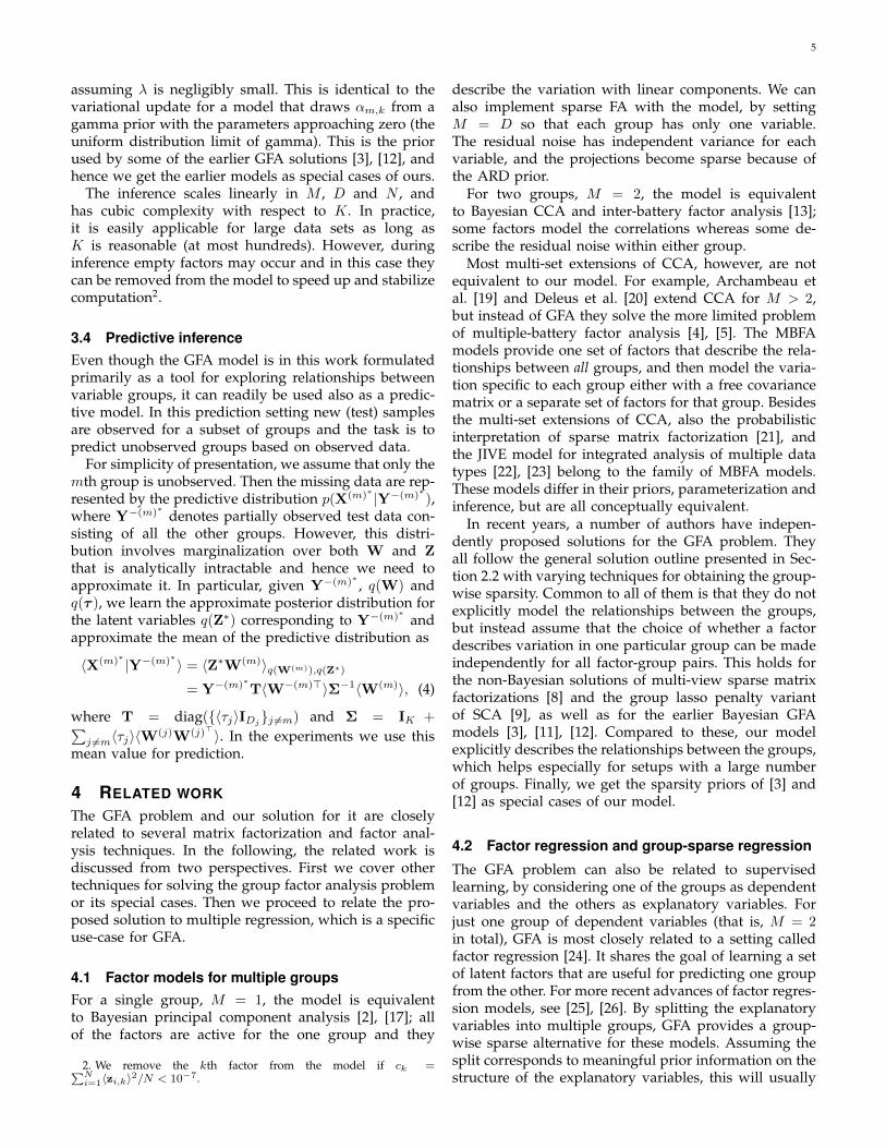
5.2 Beyond factor analysis and MBFAWe generated N = 100 samples from a GFA model withD = 30 split into M = 3 equally-sized groups. The truegenerative model had K = 7 factors, including one factorspecific for each group as well as for each possible subsetbetween the groups. Figure 3 shows the true model aswell as the solutions found by the proposed GFA model(using R = min(M,K) = 3), MBFA, and both regularand sparse FA. The proposed model finds the correctstructure, whereas MBFA suggests spurious correlations;each factor describing correlation between just two ofthe groups is falsely indicating activity also in the thirdone, according to the MBFA specification. The regularFA result is simply considerably noisier overall, whilesparse FA suffers from a few false factor loadings. Forthis simple demonstration SCA learns the same result asGFA, after manually optimizing the thresholding of com-ponent activity. For all methods we set K to a sufficientlylarge number, allowing ARD to prune out unnecessarycomponents, chose the best solution by comparing thelower bounds of 10 runs with random initializations, andfor illustrative purposes ordered the components basedon their similarity (cosine) with the true ones.

The conclusion of this experiment is that the proposedmethod indeed solves the GFA problem, whereas theMBFA and FA solutions do not provide as intuitive andinterpretable factors. For this data GFA with R < 3(not shown) fails to unveil the underlying (full-rank)structure. Instead, the loadings lie between those of GFAand FA of Figure 3, which is understandable since FA isclosely related to GFA with R = 0.

5.3 Performance for several groupsNext we studied how well the proposed solution scalesup for more groups. We generated N = 30 samples froma GFA model with K = 18 true factors. We used Dm = 7

7

Group 3

Group 2

Group 1

True

Fea

ture

s

GFA (R=3)

Fea

ture

s

MBFA

Fea

ture

s

sFA

Fea

ture

s

FA

Fea

ture

s

Fig. 3. The projections W for the true generating model, the proposed GFA solution (using full rank, R = 3), andcomparison methods multiple-battery factor analysis (MBFA), sparse factor analysis (sFA), and regular factor analysis(FA). GFA finds the true solution, whereas the other methods report spurious correlations (red boxes). The three sub-blocks in each matrix correspond to the three groups of variables, and the areas of the black patches indicate theabsolute values of the corresponding weights.

1.5

2.0

2.5

3.0

10 20 30 40 100Groups

Pre

dict

ion

RM

SE

●

●

●●

● ● ● ● ● ●●

●

GFA (R=4)GFA (R=M)MBFAFA

sFAMLRgrLassoSCA

●●●●●●●●●●●●●●●●

●

●●●●

●

●

●

●●●●●●●●●●●●●●●●

Component

Car

dina

lity

10 20 30 40

050 ● ● ● ● ● ● ● ● ● ● ● ● ● ● ● ●

●●

●

●● ● ● ● ● ● ● ● ● ● ● ● ● ● ● ● ● ● ● ●

●

●

GFA (R=4)GFA (R=M) ●

●

●●

●

●

●

●

●

●

●●

●●

●

●●●

●●

●●

●

●●

●●●

●

●

●

●

●

●

●

●

●

●

●

●

●●●

●

●

●

●●

●●

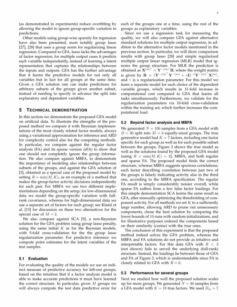
Fig. 4. Left: GFA is considerably better in modeling the relationships between the groups compared to MBFA, FA andSCA; the y-axis shows the average prediction error for a new group on the test data, providing an indirect qualitymeasure. For large M explicitly modeling the relationships between the groups (R=4) helps compared to earliersolutions that make the activity decisions independently (R = min(M,K), here R=M ). GFA also outperforms standardregression models in the prediction task, with the exception of MLR for very low dimensional data. Middle: ForM = 100the R = 4 solution correctly finds the K = 18 factors that are all active in 50 groups, whereas the earlier solutionsplits some of the factors into several ones. Right: Scatter-plot of matrix U for a R=2 solution, illustrating clearly theunderlying structure of the data. Here the symbols and colors indicate the ground truth types of the groups that werenot available for the algorithm during learning.

variables for each group and let the number of groupsgrow from M = 4 to M = 100. In other words, the totaldimensionality of the data grew from D = 28 to D =700. The variable groups were divided into four typesof equal size, so that the groups within one type had thesame association strengths for all factors. This implies alow-rank structure for the associations.

For validation we used average leave-one-group-outprediction error, further averaged over 50 independentdata sets. Figure 4 (left) shows that the proposed modeloutperforms the other FA methods by a wide margin.For small M the difference between the R = 4 and

R = min(M,K) solutions are negligible, since a smallnumber of factor-group association strengths can just aswell be selected independently. For large M , however,explicitly modeling the relationships pays off and resultsin better predictions. The prediction errors for GFA mod-els with rank R between 2 and 10 are very similar, andhence for clarity, only one (R=4) is shown in Figure 4.GFA also outperforms SCA, an alternative group-sparsefactor model, for all cases except M = 8, for which thetwo methods are equal. For cases with only 4 or 8 groupsmultiple linear regression is the most accurate method,but for all other cases, when the total dimensionality

8

Model rank

Pre

dict

ion

RM

SE

0 5 10 15 20

●

● ● ● ● ● ● ● ● ● ● ● ● ● ● ● ● ● ● ● ●●

●

●

●●

●● ● ● ● ● ● ● ● ● ●

● ● ● ● ● ●●

●

●

●

●

●

●

● ● ● ● ● ● ● ● ● ● ● ● ● ● ●●

Model rank

Low

er b

ound

0 5 10 15 20

●

●

● ● ● ● ● ● ● ● ● ● ● ● ● ● ● ● ● ● ●●

●

●

●

●

●● ● ● ● ● ● ● ● ● ● ● ● ● ● ● ●●

●

●

●

●

●●

●● ● ● ● ● ● ● ● ● ● ●

● ● ●●

●

●

●

●

Data rank 2Data rank 6Data rank 10Correct rank

Model rank

Com

p. ti

me

[s]

0 5 10 15 20

050

0

●

● ● ●●

● ● ● ● ● ● ●● ●

● ●● ● ●

● ●

●●

● ●●

●●

●●

● ●●

● ● ● ● ● ●

●●

●

●

●●

●

●

●●

●

●

●●

●● ●

●●

● ●● ● ●

● ●

●

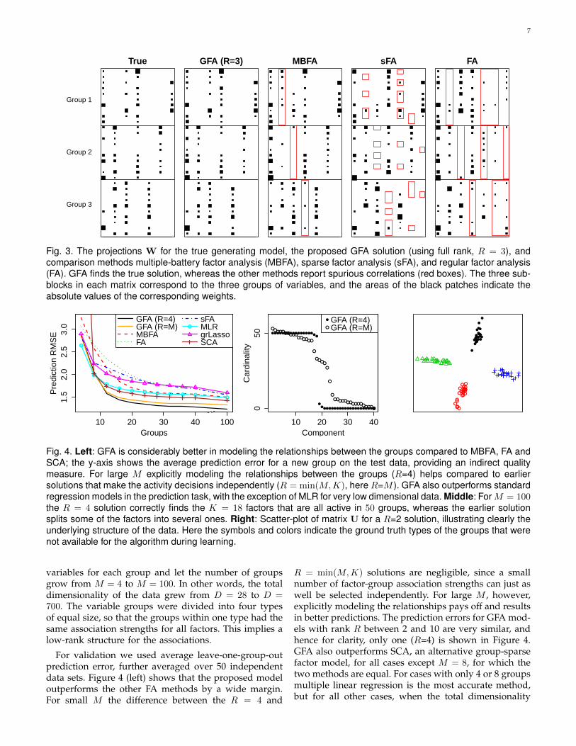
Fig. 5. The 5-fold cross-validation prediction performances (left), lower bounds (middle) and computation times(right) for three different artificial data sets as a function of the model rank R. Both approaches provide a reliableway for choosing the rank R. In the illustrated example the chosen model ranks using cross-validation are 2, 8, and10 (correct: 2, 6 and 10). By monitoring the lower bounds the true ranks, used to generate the data sets, can beapproximately detected from the figure. For clarity, the vertical positions of prediction and lower bound curves werehere altered, retaining the relative changes. The right subplot illustrates the computational cost as a function of therank R, compared against the full-rank solution shown as horizontal lines.

increases, GFA clearly outperforms also these supervisedmethods.

Besides showing better prediction accuracy, the low-rank solution (here R = 4) captures the underlyinggroup structure better than the naive model of R =min(M,K). Figure 4 (middle) compares the two byplotting the number of groups active in each factor forthe case with M = 100. There are K = 18 factors thatshould each be active in 50 groups. With R = 4 we findalmost exactly the correct solutions, whereas the naivemodel finds K = 40 factors, many of which it believesto be shared by only 5 − 40 groups. In other words, ithas split some real factors into multiple ones, finding alocal optimum, due to making all the activity decisionsindependently. For illustrative purposes, the componentswere considered active if the corresponding α-valueswere below 10. The cardinality plot is sensitive to thethreshold, but the key result stays the same regardlessof the threshold: inferring the component activities in-dependently results in a less accurate model.

Finally, Figure 4 (right) illustrates the relationshipsbetween the groups as a scatter plot of the latent factorsfor the R = 2 solution, revealing clearly the four typesof variable groups.

5.4 Choosing the model rank

GFA contains a free parameter R and this value needs tobe specified by the user. Acknowledging that choosingthe correct model order is in general a difficult problem,we resort to demonstrating two practical approaches thatseem to work well for the proposed model. The firstchoice is L-fold cross-validation within the training set,using the predictive performance for left-out groups asthe validation criterion.

A computationally more efficient alternative is to usethe ’elbow’-principle for the variational lower boundsL(Θ) computed for different choices of R. The bounds

improve monotonically3 as a function of R, but fortypical data sets the growth rate rapidly diminishes afterthe correct rank, producing an ’elbow’.

We tested both of these principles for 50 independentartificial data sets generated from the GFA model withparameters N = 50, K = 30, M = 50 and Dm = 10, forthree different data ranks: R = {2, 6, 10}, representingthe kinds of values one would typically expect for realapplications. The prediction and lower bound curves asa function of model rank are shown for a representativeexample in Figure 5. In the 5-fold cross-validation thecorrect rank was found correctly with over half of thedata sets, and the most common error was overestimat-ing the rank by one. The computationally lighter ’elbow’-principle allows the analyst to choose roughly the correctrank by simply comparing the lower bounds.

The rank R influences also the computation time, asillustrated in Figure 5. The computation time increasesroughly linearly as a function of R, but for ranks smallerthan the optimal the algorithm requires more iterationsfor convergence which slows it down. In this experiment,the low-rank model is slower than the special caseupdating α in closed form, but only by a small factor.In the real data experiments reported in Sections 6 and7 the low-rank variant was slightly faster to computefor all the tested values of R; the relative time spent onupdating α becomes small for larger data, and the low-rank models prune out excess factors faster.

In the remaining experiments we do not explicitlyselect a particular value for R, but instead present theresults for a range of different values. This is done toillustrate the relative insensitivity of the model for theprecise choice; for both real-world applications a widerange of values outperform the alternative models andalso the special case of R = min(M,K), implying thatpicking exactly the right rank is not crucial.

3. Given that the constant terms in the priors of U and V areignored.

9

N=30

Rank

Pre

dict

ion

RM

SE

0.66

0.70

0.74

0 3 6 9 M

● ● ● ● ● ● ● ● ● ● ● ●

N=120

RankP

redi

ctio

n R

MS

E0.

520.

540.

560.

58

0 3 6 9 M

● ● ● ● ● ● ● ● ● ● ● ●

●

GFAMBFAFAsFAMLRgrLassoSCA

Frontal and parietal lobes

Temporal and limbic lobes

Occipital lobe

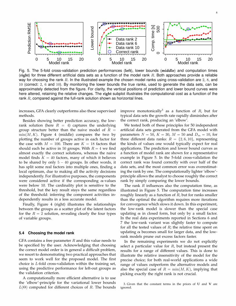
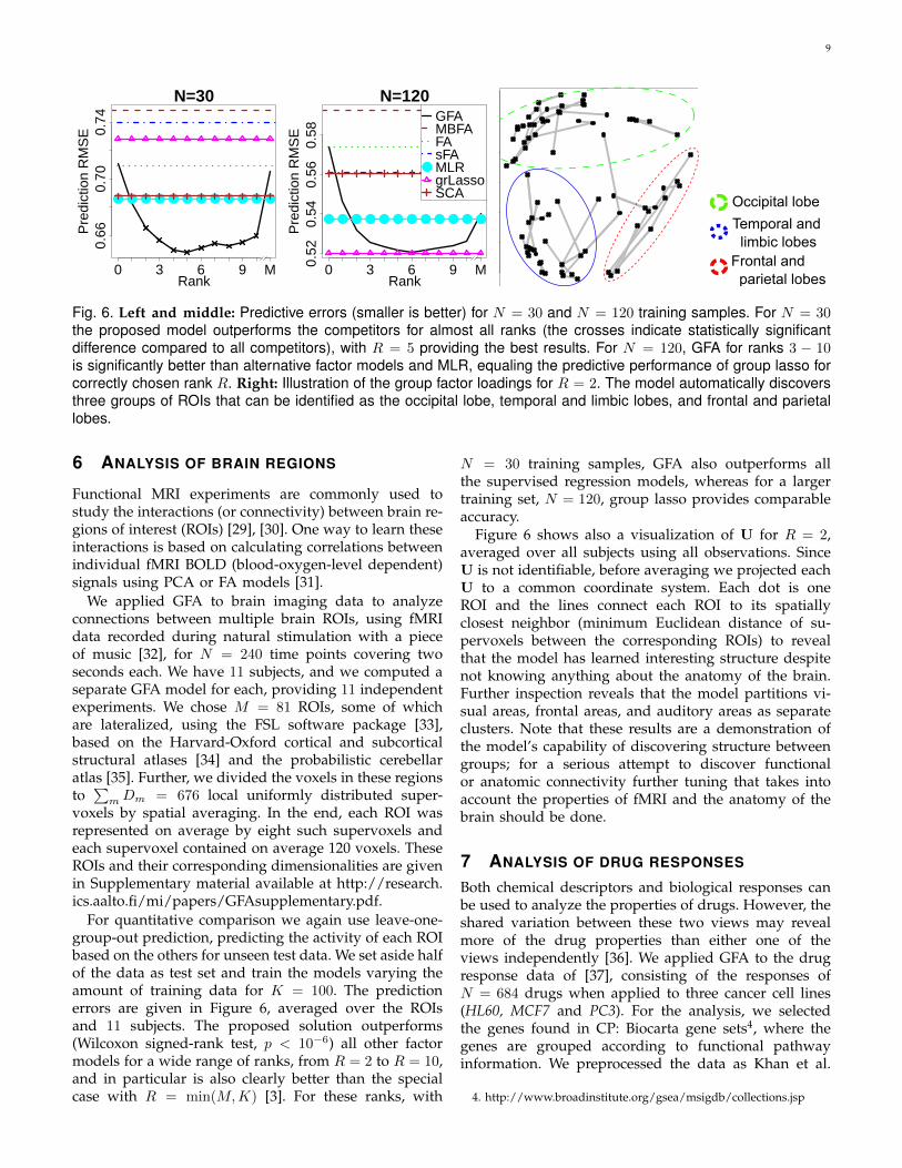
Fig. 6. Left and middle: Predictive errors (smaller is better) for N = 30 and N = 120 training samples. For N = 30the proposed model outperforms the competitors for almost all ranks (the crosses indicate statistically significantdifference compared to all competitors), with R = 5 providing the best results. For N = 120, GFA for ranks 3 − 10is significantly better than alternative factor models and MLR, equaling the predictive performance of group lasso forcorrectly chosen rank R. Right: Illustration of the group factor loadings for R = 2. The model automatically discoversthree groups of ROIs that can be identified as the occipital lobe, temporal and limbic lobes, and frontal and parietallobes.

6 ANALYSIS OF BRAIN REGIONS

Functional MRI experiments are commonly used tostudy the interactions (or connectivity) between brain re-gions of interest (ROIs) [29], [30]. One way to learn theseinteractions is based on calculating correlations betweenindividual fMRI BOLD (blood-oxygen-level dependent)signals using PCA or FA models [31].

We applied GFA to brain imaging data to analyzeconnections between multiple brain ROIs, using fMRIdata recorded during natural stimulation with a pieceof music [32], for N = 240 time points covering twoseconds each. We have 11 subjects, and we computed aseparate GFA model for each, providing 11 independentexperiments. We chose M = 81 ROIs, some of whichare lateralized, using the FSL software package [33],based on the Harvard-Oxford cortical and subcorticalstructural atlases [34] and the probabilistic cerebellaratlas [35]. Further, we divided the voxels in these regionsto∑mDm = 676 local uniformly distributed super-

voxels by spatial averaging. In the end, each ROI wasrepresented on average by eight such supervoxels andeach supervoxel contained on average 120 voxels. TheseROIs and their corresponding dimensionalities are givenin Supplementary material available at http://research.ics.aalto.fi/mi/papers/GFAsupplementary.pdf.

For quantitative comparison we again use leave-one-group-out prediction, predicting the activity of each ROIbased on the others for unseen test data. We set aside halfof the data as test set and train the models varying theamount of training data for K = 100. The predictionerrors are given in Figure 6, averaged over the ROIsand 11 subjects. The proposed solution outperforms(Wilcoxon signed-rank test, p < 10−6) all other factormodels for a wide range of ranks, from R = 2 to R = 10,and in particular is also clearly better than the specialcase with R = min(M,K) [3]. For these ranks, with

N = 30 training samples, GFA also outperforms allthe supervised regression models, whereas for a largertraining set, N = 120, group lasso provides comparableaccuracy.

Figure 6 shows also a visualization of U for R = 2,averaged over all subjects using all observations. SinceU is not identifiable, before averaging we projected eachU to a common coordinate system. Each dot is oneROI and the lines connect each ROI to its spatiallyclosest neighbor (minimum Euclidean distance of su-pervoxels between the corresponding ROIs) to revealthat the model has learned interesting structure despitenot knowing anything about the anatomy of the brain.Further inspection reveals that the model partitions vi-sual areas, frontal areas, and auditory areas as separateclusters. Note that these results are a demonstration ofthe model’s capability of discovering structure betweengroups; for a serious attempt to discover functionalor anatomic connectivity further tuning that takes intoaccount the properties of fMRI and the anatomy of thebrain should be done.

7 ANALYSIS OF DRUG RESPONSES

Both chemical descriptors and biological responses canbe used to analyze the properties of drugs. However, theshared variation between these two views may revealmore of the drug properties than either one of theviews independently [36]. We applied GFA to the drugresponse data of [37], consisting of the responses ofN = 684 drugs when applied to three cancer cell lines(HL60, MCF7 and PC3). For the analysis, we selectedthe genes found in CP: Biocarta gene sets4, where thegenes are grouped according to functional pathwayinformation. We preprocessed the data as Khan et al.

4. http://www.broadinstitute.org/gsea/msigdb/collections.jsp

10

R=2

Component

Gro

up

100200300400

100 200 300

R=K

Component100 200 300

activ

ein

activ

e

●

●

●

●

●

●

●

●

●

●

●●

●

●

●

VSHL60

MCF7PC3

Ave

rage

pre

cisi

on0.

100.

200.

30

● ● ● ● ● ● ● ● ● ● ●

●GFAMBFAFAsFA

VSGESCA

0.70

0.76

Pre

dict

ion

RM

SE

Rank0 3 6 9 M

● ● ● ● ● ● ● ● ● ● ● ●

●GFAMBFAFAsFA

MLRgrLassoSCA

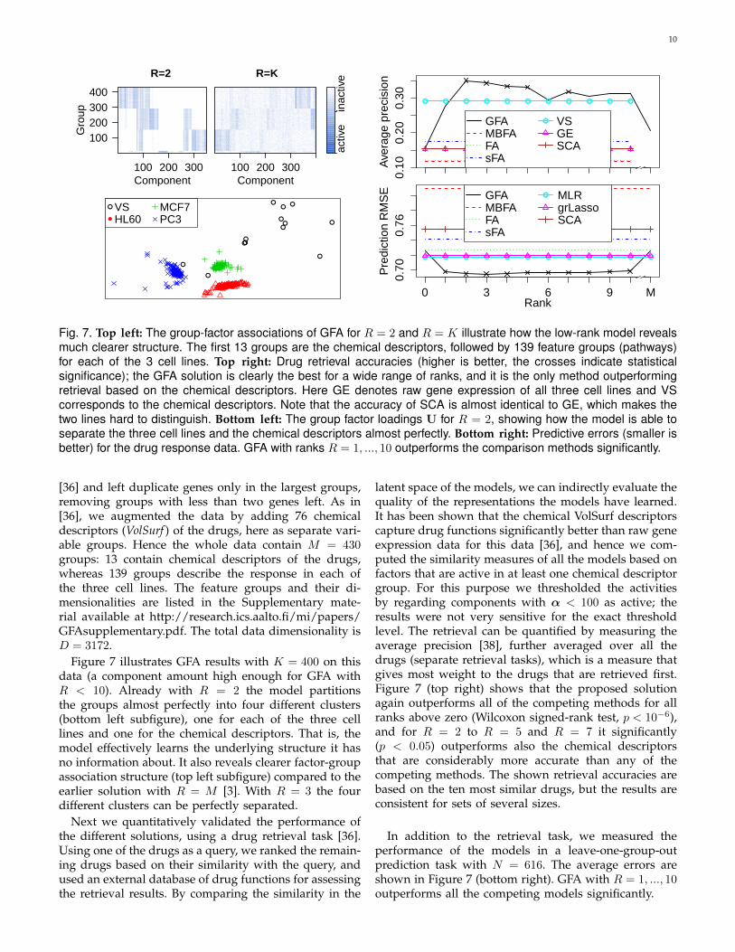
Fig. 7. Top left: The group-factor associations of GFA for R = 2 and R = K illustrate how the low-rank model revealsmuch clearer structure. The first 13 groups are the chemical descriptors, followed by 139 feature groups (pathways)for each of the 3 cell lines. Top right: Drug retrieval accuracies (higher is better, the crosses indicate statisticalsignificance); the GFA solution is clearly the best for a wide range of ranks, and it is the only method outperformingretrieval based on the chemical descriptors. Here GE denotes raw gene expression of all three cell lines and VScorresponds to the chemical descriptors. Note that the accuracy of SCA is almost identical to GE, which makes thetwo lines hard to distinguish. Bottom left: The group factor loadings U for R = 2, showing how the model is able toseparate the three cell lines and the chemical descriptors almost perfectly. Bottom right: Predictive errors (smaller isbetter) for the drug response data. GFA with ranks R = 1, ..., 10 outperforms the comparison methods significantly.

[36] and left duplicate genes only in the largest groups,removing groups with less than two genes left. As in[36], we augmented the data by adding 76 chemicaldescriptors (VolSurf ) of the drugs, here as separate vari-able groups. Hence the whole data contain M = 430groups: 13 contain chemical descriptors of the drugs,whereas 139 groups describe the response in each ofthe three cell lines. The feature groups and their di-mensionalities are listed in the Supplementary mate-rial available at http://research.ics.aalto.fi/mi/papers/GFAsupplementary.pdf. The total data dimensionality isD = 3172.

Figure 7 illustrates GFA results with K = 400 on thisdata (a component amount high enough for GFA withR < 10). Already with R = 2 the model partitionsthe groups almost perfectly into four different clusters(bottom left subfigure), one for each of the three celllines and one for the chemical descriptors. That is, themodel effectively learns the underlying structure it hasno information about. It also reveals clearer factor-groupassociation structure (top left subfigure) compared to theearlier solution with R = M [3]. With R = 3 the fourdifferent clusters can be perfectly separated.

Next we quantitatively validated the performance ofthe different solutions, using a drug retrieval task [36].Using one of the drugs as a query, we ranked the remain-ing drugs based on their similarity with the query, andused an external database of drug functions for assessingthe retrieval results. By comparing the similarity in the

latent space of the models, we can indirectly evaluate thequality of the representations the models have learned.It has been shown that the chemical VolSurf descriptorscapture drug functions significantly better than raw geneexpression data for this data [36], and hence we com-puted the similarity measures of all the models based onfactors that are active in at least one chemical descriptorgroup. For this purpose we thresholded the activitiesby regarding components with α < 100 as active; theresults were not very sensitive for the exact thresholdlevel. The retrieval can be quantified by measuring theaverage precision [38], further averaged over all thedrugs (separate retrieval tasks), which is a measure thatgives most weight to the drugs that are retrieved first.Figure 7 (top right) shows that the proposed solutionagain outperforms all of the competing methods for allranks above zero (Wilcoxon signed-rank test, p < 10−6),and for R = 2 to R = 5 and R = 7 it significantly(p < 0.05) outperforms also the chemical descriptorsthat are considerably more accurate than any of thecompeting methods. The shown retrieval accuracies arebased on the ten most similar drugs, but the results areconsistent for sets of several sizes.

In addition to the retrieval task, we measured theperformance of the models in a leave-one-group-outprediction task with N = 616. The average errors areshown in Figure 7 (bottom right). GFA with R = 1, ..., 10outperforms all the competing models significantly.

11

8 DISCUSSION

Joint analysis of multiple data sets is one of the trendsin machine learning, and integrated factor analysis ofmultiple real-valued matrices is one of the prototypicalscenarios for that task. In recent years multiple authorshave re-discovered the multiple-battery factor analysis(MBFA) task originating from the early works in statistics[4], [5], [6], [7], calling it either multi-set CCA [19],[20], or simply as a model for integrated analysis ofmultiple data sources [22], [23]. Despite varying technicaldetails, all of these models can be seen as FA modelswith two sets of factors: one set describes dependenciesbetween all of the variable groups, whereas the otherset describes, or explains away, variation specific to eachgroup.

The group factor analysis problem formulated in thisarticle, extending the preliminary treatment in [3], differsfrom the MBFA models in one crucial aspect. Instead ofonly modeling relationships between all of the groups,we also introduce factors that model relationships be-tween any subset of them. While some other recentworks [8], [9], [11], [12] have also addressed the sameproblem, in this paper the GFA setup is for the first timeintroduced explicitly, putting it into its statistical context.We described a general solution principle that covers theearlier solutions, identifying the structural sparsity prioras the key element. We then presented a more advancedsparsity prior that results in a novel GFA solution:Instead of choosing the activities of each group-factorpair independently, we explicitly model the relationshipsbetween the groups with another linear layer. Our modelhence directly provides factor loadings also betweenthe groups themselves, which was exactly the originalmotivation for the GFA problem. Our preliminary model[3] is a special case with a priori independent loadings.

We showed, using artificial data, how the GFA prob-lem and solution differ from the MBFA-problem andclassical FA. We also demonstrated that, especially for alarge number of groups or data sets, it pays off to explic-itly model the relationships between the groups. Finally,we applied the model on two real-world exploratoryanalysis scenarios in life sciences. We demonstratedthat the model is applicable to connectivity analysis offMRI data, as well as for revealing structure shared bystructural description of drugs and their response inmultiple cell lines. These demonstrations illustrated thekinds of setups the GFA is applicable for, but shouldnot be considered as detailed analyses of the specificapplication problems.

Besides showing that the proposed model solves theGFA problem considerably better than the alternativesMBFA, FA and SCA [9], the empirical experiments re-vealed that there is a qualitative difference betweenthe proposed model having the more advanced struc-tural sparsity prior and the earlier GFA solutions suchas [3]. Even though the earlier models also solve theGFA problem reasonably well, they are outperformed

by supervised regression models in predictive tasks.The proposed solution with a low-rank model for thegroup association strengths is clearly more accurate inprediction tasks and, at least for small training sets,outperforms also dedicated regression models trainedspecifically to predict the missing groups. This is a strongresult for a model that does not know in advance whichgroups correspond to explanatory variables and which tothe dependent variables, but that instead learns a singlemodel for all possible choices simultaneously.

The model presented here is limited to scenarios whereeach training sample is fully observed. Support formissing observations could be added using the fullyfactorized variational approximation used for PCA andcollective matrix factorization with missing data [17],[39]. A similar approach can also be used for semi-paired setups where some samples are available onlyfor some groups [40], by filling in the remaining groupsby missing observations. Empirical comparisons on theseare left for future work. Another possible direction forfuture work concerns more justified inference for therank parameter R; even though the experiments heresuggest that the method is robust to the choice, themethod would be more easily applicable if it was se-lected automatically.

ACKNOWLEDGMENT

We thank the Academy of Finland (grant numbers140057, 266969, and 251170; Finnish Centre of Excel-lence in Computational Inference Research COIN), theaivoAALTO project of Aalto University, and Digile ICTSHOK (D2I programme) for funding the research. Wewould also like to thank Suleiman A. Khan for his helpwith the biological application, and Enrico Glerean forhis help with the neuroscience application. We acknowl-edge the computational resources provided by AaltoScience-IT project.

REFERENCES[1] L. Thurstone, “Multiple factor analysis,” Psychological Review,

vol. 38, no. 5, pp. 406–427, 1931.[2] C. M. Bishop, “Bayesian PCA,” Advances in Neural Information

Processing Systems, vol. 11, pp. 382–388, 1999.[3] S. Virtanen, A. Klami, S. A. Khan, and S. Kaski, “Bayesian group

factor analysis,” Proc. 15th Int. Conf. Artificial Intelligence andStatistics, pp. 1269–1277, 2012.

[4] R. McDonald, “Three common factor models for groups of vari-ables,” Psychometrika, vol. 37, no. 1, pp. 173–178, 1970.

[5] M. Browne, “Factor analysis of multiple batteries by maxi-mum likelihood,” British J. Mathematical and Statistical Psychology,vol. 33, no. 2, pp. 184–199, 1980.

[6] L. R. Tucker, “An inter-battery method of factor analysis,” Psy-chometrika, vol. 23, no. 2, pp. 111–136, 1958.

[7] M. W. Browne, “The maximum-likelihood solution in inter-batteryfactor analysis,” British J. Mathematical and Statistical Psychology,vol. 32, no. 1, pp. 75–86, 1979.

[8] Y. Jia, M. Salzmann, and T. Darrell, “Factorized latent spaceswith structured sparsity,” Advances in Neural Information ProcessingSystems, vol. 23, pp. 982–990, 2010.

[9] K. V. Deun, T. F. Wilderjans, R. A. v. Berg, A. Antoniadis, andI. V. Mechelen, “A flexible framework for sparse simultaneouscomponent based data integration,” BMC Bioinformatics, vol. 12,no. 1, pp. 448, 2011.

12

[10] S. K. Gupta, D. Phung, B. Adams, and S. Venkatesh, “A Bayesianframework for learning shared and individual subspaces frommultiple data sources,” Proc. Advances in Knowledge Discovery andData Mining, 15th Pacific-Asia Conf., PAKDD, pp. 136–147, 2011.

[11] S. K. Gupta, D. Phung, and S. Venkatesh, “A Bayesian non-parametric joint factor model for learning shared and individualsubspaces from multiple data sources,” Proc. 12th SIAM Int. Conf.Data Mining, pp. 200–211, 2012.

[12] A. Damianou, C. Ek, M. Titsias, and N. Lawrence, “Manifoldrelevance determination,” Proc. 29th Int. Conf. Machine Learning,pp. 145–152, 2012.

[13] A. Klami, S. Virtanen, and S. Kaski, “Bayesian canonical correla-tion analysis,” J. Machine Learning Research, vol. 14, no. 1, pp. 899–937, 2013.

[14] A. Klami and S. Kaski, “Probabilistic approach to detecting de-pendencies between data sets,” Neurocomputing, vol. 72, no. 1,pp. 39–46, 2008.

[15] S. Virtanen, A. Klami, and S. Kaski, “Bayesian CCA via groupsparsity,” Proc. 28th Int. Conf. Machine Learning, pp. 457–464, 2011.

[16] J. Aitchison, “The statistical analysis of compositional data,” J.Royal Statistical Society. Series B (Methodological), vol. 44, no. 2,pp. 139-177, 1982.

[17] A. Ilin, and T. Raiko, “Practical approaches to principal compo-nent analysis in the presence of missing data,” J. Machine LearningResearch, vol. 11, pp. 1957-2000, 2010.

[18] O. Dikmen and C. Fevotte, “Nonnegative dictionary learning inthe exponential noise model for adaptive music signal represen-tation,” Advances in Neural Information Processing Systems, vol. 24,pp. 2267–2275, 2011.

[19] C. Archambeau and F. Bach, “Sparse probabilistic projections,”Advances in Neural Information Processing Systems, vol. 21, pp. 73–80, 2009.

[20] F. Deleus and M. V. Hulle, “Functional connectivity analysis offMRI data based on regularized multiset canonical correlationanalysis,” J. Neuroscience Methods, vol. 197, no. 1, pp. 143–157,2011.

[21] X. Qu and X. Chen, “Sparse structured probabilistic projectionsfor factorized latent spaces,” Proc. 20th ACM Int. Conf. Informationand Knowledge Management, pp. 1389–1394, 2011.

[22] E. Lock, K. Hoadley, J. Marron, and A. Nobel, “Joint and individ-ual variation explained (JIVE) for integrated analysis of multipledatatypes,” Annals of Applied Statistics, vol. 7, no. 1, pp. 523–542,2013.

[23] P. Ray, L. Zheng, Y. Wang, J. Lucas, D. Dunson, and L. Carin,“Bayesian joint analysis of heterogeneous data,” Duke Univ.,Dept. of Elec. and Comp. Eng., Tech. Rep., 2013.

[24] M. West, “Bayesian factor regression models in the large p, smalln paradigm,” Bayesian Statistics, vol. 7, pp. 733–742, 2003.

[25] N. Chen, J. Zun, and E. Xing, “Predictive subspace learning formulti-view data: a large margin approach,” Advances in NeuralInformation Processing Systems, pp.361–369, 2010.

[26] P. Rai, and H. Daume, “The Infinite Hierarchical Factor RegressionModel,” Advances in Neural Information Processing Systems, vol. 21,pp. 1321–1328, 2009.

[27] M. Yuan, and Y. Li, “Model selection and estimation in regres-sion with grouped variables,” J. Royal Statistical Society: Series B(Statistical Methodology), vol. 68, no. 1, pp. 49–67, 2006.

[28] P. Breheny, and J. Huang, “Group descent algorithms for noncon-vex penalized linear and logistic regression models with groupedpredictors,” Statistics and Computing, pp.1–15, 2013.

[29] K. J. Friston, “Functional and effective connectivity in neuroimag-ing: a synthesis,” Human Brain Mapping, vol. 2, no. (1-2), pp. 56–78,1994.

[30] S. Smith et al., “Correspondence of the brains functional architec-ture during activation and rest,” Proc. National Academy of Sciences(PNAS), vol. 106, no. 31, pp. 13040–13045, 2009.

[31] K. Friston, C. Frith, P. Liddle, and R. Frackowiak, “Functionalconnectivity: the principal-component analysis of large (PET) datasets,”J. Cerebral Blood Flow and Metabolism, vol. 13, no. 1, pp. 5–14,1993.

[32] V. Alluri, P. Toiviainen, I. P. Jaaskelainen, E. Glerean, M. Sams,and E. Brattico, “Large-scale brain networks emerge from dy-namic processing if musical timbre, key and rhythm,” NeuroImage,vol. 59, no. 4, pp. 3677–3689, 2012.

[33] M. Jenkinson, C. Beckmann, T. Behrens, M. Woolrich, andS. Smith, “FSL,” NeuroImage, vol. 62, no. 2, pp. 782–790, 2012.

[34] R. Desikan, F. Segonne, B. Fischl, B. Quinn, B. Dickerson,D. Blacker, R. Buckner, A. Dale, R. Maguire, B. Hyman, M. Albert,and R. Killiany, “An automated labeling system for subdividingthe human cerebral cortex on MRI scans into gyral based regionsof interest,” NeuroImage, vol. 31, no. 3, pp. 980–986, 2006.

[35] J. Diedrichsen, J. Balster, E. Cussans, and N. Ramnani, “A prob-abilistic MR atlas of the human cerebellum,” NeuroImage, vol. 46,no. 1, pp. 39–46, 2009.

[36] S. A. Khan, A. Faisal, J. P. Mpindi, J. A. Parkkinen, T. Kalliokoski,A. Poso, O. P. Kallioniemi, K. Wennerberg, and S. Kaski, “Com-prehensive data-driven analysis of the impact of chemoinformaticstructure on the genome-wide biological response profiles ofcancer cells to 1159 drugs,” BMC Bioinformatics, vol. 13, no. 112,pp. 1–15, 2012.

[37] J. Lamb, E. Crawford, D. Peck, J. Modell, I. Blat, M. Wro-bel, J. Lerner, J. Brunet, A. Subramanian, K. Ross et al., “Theconnectivity map: using gene-expression signatures to connectsmall molecules, genes, and disease,” Science, vol. 313, no. 5795,pp. 1929–1935, 2006.

[38] R. Baeza-Yates, B. Ribeiro-Neto, “Modern information retrieval,”ACM Press New York, 1999.

[39] A. Klami, G. Bouchard, and A. Tripathi, “Group-sparse embed-dings in collective matrix factorization,” Proc. Int. Conf. LearningRepresentations, 2014.

[40] X. Chen, S. Chen, H. Xue, and X. Zhou, “A unified dimensionalityreduction framework for semi-paired and semi-supervised multi-view data,” Pattern Recognition, vol. 45, no. 5, pp. 2005–2018, 2012.

APPENDIX

The latent variables are updated as q(Z) =∏Ni=1N (zi|m(z)

i ,Σ(z)), where

Σ(z) =

(Ik +

M∑m=1

〈τm〉〈W(m)W(m)>〉

)−1

m(z)i =

M∑m=1

Σ(z)〈W(m)〉〈τm〉x(m)i .

The projection matrices are updated as q(W) =∏Mm=1

∏Dm

j=1N (w(m):,j |m

(w)m,j ,Σ

(w)m ), where

Σ(w)m =

(〈τm〉

N∑i=1

〈ziz>i 〉+ 〈αm〉

)−1

m(w)m,j = Σ(w)

m 〈τm〉

(N∑i=1

x(m)ij 〈zi〉

),

and αm is the mth row of α transformed into a diagonalK ×K matrix.

Noise precision q(τ ) =∏Mm=1 G(τm|aτm, bτm) parame-

ters are updated as

aτm = aτ +DmN

2

bτm = bτ +1

2

N∑i=1

⟨(x

(m)i −W(m)>zi)

2⟩.

Finally, for the low-rank model, α = eUV>+µu1>+1µ>v

is updated by optimizing the lower bound numerically.The bound as a function of U and V is given by∑

m,k

Dm log(αm,k)− 〈W(m)W(m)>〉k,kαm,k

− λ(tr(U>U) + tr(V>V)).

13

The gradients w.r.t. the cost function are given as

δL

δU= AV + λU,

δL

δµv= A1,

δL

δV= A>U + λV,

δL

δµv= A>1,

where A = D1> − exp(UV> + µu1> + 1µ>v ).

With full rank [3] the ARD parameters are updated asq(α) = G(aαm, b

αmk), where

aαm = aα +Dm

2

bαmk = bα +w

(m)>k w

(m)k

2.