group behaviors for systems with signiﬁcant dynamicsdbrogan/publications/papers/jar_herd.pdf ·...

Autonomous Robots, 4, 137--153 (1997)c 1997 Kluwer Academic Publishers, Boston. Manufactured in The Netherlands.

Group Behaviors for Systems with Significant Dynamics

DAVID C. [email protected]

College of Computing, Georgia Institute of Technology, Atlanta, GA 30332-0280

JESSICA K. [email protected]

College of Computing, Georgia Institute of Technology, Atlanta, GA 30332-0280

Received September 29, 1995. Revised September 30, 1996.

Editor: George A. Bekey

Abstract. Birds, fish, and many other animals travel as a flock, school, or herd. Animals in these groupsmust remain in close proximity while avoiding collisions with neighbors and with obstacles. We would like toreproduce this behavior for groups of simulated creatures traveling fast enough that dynamics plays a significantrole in determining their movement. In this paper, we describe an algorithm for controlling the movements ofcreatures that travel as a group and evaluate the performance of the algorithm with three simulated systems: leggedrobots, humanlike bicycle riders, and point-mass systems. Both the legged robots and the bicyclists are dynamicsimulations that must control balance, facing direction, and forward speed as well as position within the group.The simpler point-mass systems are included because they help us to understand the effects of the dynamics on theperformance of the algorithm.

Keywords: multi-agent, herds, group navigation, dynamic simulation, legged locomotion

1. Introduction

To run as a group, animals must remain in close prox-imity while avoiding collisions with other members ofthe group and with obstacles in the environment. Wewould like to create multi-agent systems that repli-cate the complexity and variability of natural groupsby using simple communication, cooperation, and co-ordination strategies. In this paper, we explore theperformance of one such algorithm for group behav-iors. The groups are made up of dynamically simulatedlegged robots, bicycle riders, and point masses. Ex-amples of the systems we have simulated are shown infigure 1.

The algorithm for group behaviors computes a de-sired position for each individual based on the locationand velocity of its visible neighbors, the location ofvisible obstacles, and a global desired group veloc-ity. Each creature’s desired position and velocity areknown only to that creature although members of thegroup can estimate this information based on their

observations of the creature’s actions. We comparethe performance of this algorithm on the three dy-namic simulations for a test suite of three problems:steady-state motion, turning, and avoiding obstacles.

The point-mass system demonstrates the most ro-bust performance in all tests because the control ex-erted by the grouping behaviors causes rapid andpredictable changes in position and velocity. Thesepredictable changes allow the point masses to navi-gate without collisions even with little advance noticeof large obstacles. Predicting the movement of one-legged robots is more difficult because their velocityvaries over a running cycle. Furthermore, the controlof velocity is not as exact for the one-legged robots asit is for the point masses. For these reasons, groupingbehaviors for the robots must compute less aggressivechanges in desired position and velocity to avoid caus-ing crashes. When the delay inherent in the controlof velocity is taken into account, however, the one-legged robots are able to complete without collisions

138 Brogan and Hodgins

Fig. 1. Images of 105 simulated one-legged robots and 5 simulated bicycle riders.

the tests of obstacle avoidance and turning presentedin this paper.

The bicyclists are the least robust of the threesystems because the underlying control system forsteering and balance is unable to execute some of thechanges in velocity and direction requested by thehigher-level algorithm for group behaviors. When thehigher-level algorithm requires better control than isavailable, individual bicyclists crash to the ground orinto another member of the group. We reduced thedifficulty of the turning test to allow the bicyclists tocomplete the tests without collisions.

In contrast to most previous implementations ofalgorithms for group behaviors, we are exploring al-gorithms for groups in which the members have sig-nificant dynamics. By significant dynamics, we meanthat the motion of each individual is significantly af-fected by its dynamic properties and that a kinematicor point-mass simulation would not be an adequaterepresentation. The dynamic system for an individualcreates inherent limitations on acceleration, velocity,and turning radius. These limitations restrict what thelow-level control algorithms can do and result in tran-sient and steady-state errors. For example, changesin velocity of the one-legged robots may be delayedby almost a full running cycle because the low-levelcontrol system can influence velocity only during thestance phase of the cycle. The bicyclists also experi-ence a delay because in order to turn to the right theymust first steer to the left and lean right.

Algorithms for higher-level behaviors are neededfor the construction of cooperating robots with robustand agile movements. When a robot moves quickly

enough that the dynamics of the system plays a sig-nificant role in the resulting motion, the algorithmthat controls the higher-level behaviors must includeexplicit models of both the underlying dynamics andthe limitations of the low-level control. It is our hopethat by exploring the performance of this algorithmon dynamically simulated creatures, we can gain anunderstanding of principles that will carry over to thecontrol of groups of physical robots performing usefultasks.

Algorithms for higher-level behaviors are alsoneeded for the construction of virtual actors that canmove and interact with a dynamic environment ro-bustly and realistically. A dynamic simulation in con-cert with a control system will provide natural-lookingmotion for such low-level behaviors as walking, run-ning, bicycling, and climbing. Higher-level behaviorssuch as obstacle avoidance, grouping, and rough ter-rain locomotion would allow the actor to interact withthe user and with a complex and unpredictable envi-ronment.

2. Background

Herding, flocking, and schooling behaviors of animalshave been studied extensively over the past century,and this research has stimulated attempts to createrobots and simulated creatures with similar skills. Bi-ologists have found that groupings in animals arecreated through an attraction that modulates the desireof each member to join the group with the desire tomaintain a sufficient distance from nearby creatures(Shaw, 1970). As an example of this attraction, Cullen,

Group Behaviors for Systems with Significant Dynamics 139

Shaw, and Baldwin (1965) report that the density offish is approximately equal in all planes of a school,as if each fish had a sphere around its head with whichit wished to contact the spheres of other fish. Biolo-gists have found that herding benefits group membersby limiting the average number of encounters withpredators (data summarized in Veherencamp (1987)).Group behaviors also allow animals to hunt morepowerful animals than those they could overpower asindividuals. The success of behaviors such as these inbiological systems argues the merit of exploring theiruse in robotic systems. An understanding of thesebehaviors is essential for realistic creatures in virtualenvironments.

Early progress in the simulation of group behaviorswas made by Reynolds (1987). Actors in his systemare birdlike objects similar to the point masses usedin particle systems except that each bird also has anorientation. The birds maintain proper position andorientation within the flock by balancing their desireto avoid collisions with neighbors, to match the ve-locity of nearby neighbors, and to move towards thecenter of the flock. Each bird uses only informationabout nearby neighbors. This localization of informa-tion simulates one aspect of perception and reactionin biological systems and helps to balance the threeflocking tendencies. Reynolds’s work demonstratesthat realistic-looking animations of group formationscan be created by applying simple rules to determinethe behaviors of the individuals in the flock.

Yeung and Bekey (1987) proposed a decentralizedapproach to the navigation problem for multiple agents.Their simulation system first constructs a global planwithout taking into account moving obstacles. Whena collision is imminent, the system locally replans us-ing interrobot communication to resolve the conflict.Because of the two levels of planning, this solutionrequires the communication overhead associated withgroup behaviors only when a pair of robots perceivean impending collision.

Sugihara and Suzuki (1990) demonstrated that mul-tiple robots can form stable formations in simulationwhen each robot executes an identical algorithm forposition determination within the group. Each robotcan perceive the relative positions of all other robotsand has the ability to move one grid position duringeach unit of time. By adjusting the position of eachrobot relative to either the most distant or the closestneighbor, a regular geometric shape such as a circle can

be formed by the robots in the simulation. By carefullyconstructing the algorithm that each robot uses in de-termining intragroup position, formations will emergewithout a priori knowledge about the total number ofrobots. Designation of leaders allows the simple rulesof the group to create leader-follower algorithms andto demonstrate the division of a formation into smallergroups.

Wang (1991) investigated the asymptotic stabilityof multiple simulated robots in formation. Each robotin the model is simulated as a point mass and per-ceives other robots in the region contained in a coneextending from the center of the robot and heading inthe direction of travel. Formations are represented as aset of offsets from a predefined reference robot. In thisway, a formation can be directly defined as a set ofpositions for each robot relative to the leader, closestneighbor, or set of closest neighbors. Wang provedthat the error in desired position relative to actual po-sition diminishes to zero for each independent robotin the formation and therefore the desired formation isasymptotically stable.

Takeuchi, Unuma, and Amakawa (1992) imple-mented path planning in simulated multi-agent sys-tems where the attraction between agents is dependenton properties of the agents. The simulated agents areNewtonian particles where forces are applied to theagents based on the vector sum of attractions to otherobservable agents. This method was used to formulatea path for a butterfly among flowers, to describe thepaths of schooling fish when approached by a predator,and to generate the paths of humans avoiding a car.

Arkin explored the question of communication ina group of interacting mobile robots in the laboratoryusing schema-based reactive control ((Arkin, 1992),(Arkin and Hobbs, 1992)). Example schemas aremove-to-goal, move-ahead, and avoid-static-obstacle.Each behavior computes a velocity vector that is com-bined with the velocity vectors from the other behav-iors. The combined velocity vector is used to controlthe robot. Arkin demonstrated that multiple robots caneffectively complete group tasks such as foraging andcan retrieve large quantities of goal items with little orno explicit communication. The algorithm for groupbehaviors described in this paper is similar to Arkin’sapproach in that it is an example of an algorithm inwhich there is no explicit leader and all communicationis through observations of the environment.


A Black creatures canbe seen by A

Fig. 2. One creature is visible to another if it is one of the n closestcreatures (n is 6 for this example). The black circles represent theset of visible creatures, N , and the white those that cannot be seenby A.

Mataric explored emergent behavior and group dy-namics in a group of 20 wheeled vehicles in thelaboratory. These robots, like Arkin’s, do not explic-itly communicate state or goals and the system has noleaders. This work demonstrated that combinations ofsuch simple behaviors as aggregation and dispersioncan produce such complex relationships as flockingin physical robots in the laboratory ((Mataric, 1992a),(Mataric, 1992b)). The robots utilize the knowledgethat they are all identical when executing behaviors, butan extension to these results found that heterogeneousagents do not perform significantly better than homo-geneous ones (Mataric, 1993). In these experiments,a hierarchy is created in which an ordering betweenthe agents determines which agent will move first incompleting such tasks as grouping and dispersing.

Parker (1993) investigated the advantages and dis-advantages of using local and global knowledge whendesigning control laws for cooperative agent teams.Simulated wheeled robots were used to explore thetradeoffs in tasks where the robots are commandedto move in formation. She found that knowledge ofglobal goals and global state contributes to improvedperformance but at the cost of increased interagentcommunication. Behavioral analysis is an alternativeto communicating global knowledge when the actionsof the agents are recognizable. The experiments indi-cate that global knowledge should be used to controllonger-term actions whereas local knowledge is bestused to control short-term actions that fit within thecontext of global goals. In this way, local informationgrounds the global knowledge in the current robotstate.

3. Group Behaviors

The algorithm for group behaviors described in thispaper was evaluated on three simulated systems: a

D

d

1

2 3

1

global desired position(weighted average), x

desired position withrespect to this creature, x

d

d(3)

Fig. 3. The locations of the visible creatures are used to compute aglobal desired position for the individual under consideration. Thealgorithm computes a desired position with respect to each visiblerobot, xd(i), by finding the point on the line between the individualand the visible creature that is a constant distance D away fromthe visible creature. These desired positions are averaged with aweighting equal to 1=d2i where di is the distance between the twocreatures.

one-legged robot, a rigid-body model of a human rid-ing a bicycle, and a point-mass system. In most trialsthe groups of point-mass systems and of legged robotseach contained 105 individuals; the group of bicyclistscontained 18 individuals.

The algorithm for group behaviors has two parts: aperception model to determine the creatures and ob-stacles visible to each individual in the group and aplacement algorithm to determine the desired positionfor each individual given the locations and velocitiesof the visible creatures and obstacles. The low-levelcontrol algorithms for each creature use the desired po-sition to compute a desired velocity and then attemptto achieve that velocity.

Each individual in a group can perceive the relativelocations and velocities of the set of visible creatures,N (figure 2). This information is used to compute adesired position, (xd(i); yd(i)), relative to each of thesecreatures. This position is a distance D away from thevisible creature on the line between the two creatures(figure 3):

y =yi � yA

xi � xAx (1)

where (xi; yi) is the current position of creature i, and(xA; yA) is the current position of creature A. Whenxi = xA, the two creatures are on a line parallel tothe y axis and the slope of the line is assumed to be a


A

1

2

3

Obstacle

Desired position for creature A is3

Direction of Travel

Desired position relative tothe obstacle

meters from desiredDposition relative to the obstacle

off

Fig. 4. The desired position for creature A takes into account boththe obstacle and the neighbors that will move sideways as theyapproach the obstacle. First, the algorithm calculates a desiredposition that will prevent the creature from hitting the obstacle.Then the algorithm creates a rectangular region between creatureAand the obstacle, calculates the number of visible neighbors withinthat region, and multiplies the desired separation distance, Doff ,by the number of creatures. In the figure, creatures 1; 2; and 3

are members of n and are contained within the shaded rectangularregion, so Doff is multiplied by three and that amount is added tothe desired position with respect to the obstacle.

large, but not infinite, number. The desired separationdistance, D, specifies that (xd(i); yd(i)) is D metersaway from creature i:

D =

qxd(i)

2 + y2d(i): (2)

Using equations 1 and 2, we can solve for (xd(i); yd(i)):

xd(i) =Dr�

yi�yAxi�xA

�2+ 1

: (3)

yd(i) is computed in a similar fashion. After computingthe desired position relative to each creature in N , theset of desired positions is weighted by the actual dis-tance between each pair of creatures, di, and averagedto compute a global desired position:

xd = xA +

Xi2N

sgn(xA � xi)xd(i)

di2

Xi2N

1di

2

: (4)

sgn(p) returns -1 when p is negative and 1 otherwise.The desired y position, yd, is computed similarly.

In addition to avoidingcollisionswith other individ-uals in the group, the creatures must avoid obstacles.The effect of an obstacle on a creature’s behavior in-creases as it nears the obstacle, and an offset to the leftor right of the obstacle is added to the average of thedesired positions relative to neighbors:

ydobs = yobs �Dobs

d2obs� yA (5)

where yobs is the y position of the obstacle, Dobs isthe desired separation distance from the obstacle, anddobs is the actual distance between the creature andthe obstacle. In addition, the algorithm for groupingbehaviors allows space between the creature and theobstacle for the creature’s neighbors by calculatingthe number of visible neighbors between the creatureand the obstacle and multiplying this number by anadditional separation distance, Doff , to produce anadditional offset to the desired position for avoidingthe obstacle (figure 4).

After the individual passes the center of the ob-stacle, the average of the desired positions relative toneighbors includes a term for a position towards thecenter of the obstacle. This term serves to bring the twogroups on either side of the obstacle together. Withina short distance, the two groups perceive and react tocreatures from the other group, merge into one, andreturn to steady state.

Although the group behaviors are identical for thethree systems up to this point in the algorithm, thesystems use the information about desired position indifferent ways. The one-legged robots and the bicy-clists adjust speed and facing direction in an attemptto eliminate the error in position. In contrast, the errorin desired position for the point masses is reduced byapplying a force to the point mass. These differencesare described in detail in the following sections.

4. Simulating Groups

A simulation of a group of creatures consists of theequations of motion and a state vector for each crea-ture, control algorithms for running or bicycling, agraphical image for viewing the motion of the group,and an interface that allows the user to control theparameters of the simulation. For the group of robots,each simulation includes the equations of motion fora rigid-body model of a one-legged robot and controlalgorithms that allow the robot to run at a variety ofspeeds and flight durations. For the group of bicyclists,each simulation includes the equations of motion fora rigid-body model of the bicycle and humanlike riderand the control algorithms for steering and propellingthe bike forward.

The equations of motion for the robot and the bicy-clist were formulated using a commercially available


zy

x

hip (x, y, z rotation)

y rotationof hip

leg length

Fig. 5. The reference angles for the degrees of freedom of theone-legged robot. The controlled degrees of freedom are the threedegrees of freedom at the hip and the length of the leg.

package (Rosenthal and Sherman, 1986). The equa-tions of motion for the individuals in the group do nottake into account the physical effects of collisions be-tween two members of the group, although collisionsare detected and a count of collisions is recorded foruse in analyzing the data. There were no collisionsin the tests described in this paper. The details of therobot, the bicycle rider, and the point-mass models aredescribed below.

4.1. One-legged Robot

The locomotion algorithm for the one-legged robotcontrols flight duration, body attitude, and forwardand sideways velocity. Flight duration is controlled byextending the telescoping leg during stance to makeup for losses in the system:

ld = ltd + lth (6)

where ld is the desired length of the leg, ltd is the lengthof the leg at touchdown, and lth is the desired thrust.Body attitude (pitch, roll, and yaw) is controlled byexerting a torque between the body and the leg duringstance:

�� = k�(�d � �) � k _�_� (7)

where � is the pitch, roll, or yaw angle, �� is thehip torque for the corresponding axis, k� is the pro-portional gain, k _� is the derivative gain, �d is thedesired angle, and _� is the roll, pitch or yaw velocity.The forward and sideways velocities are controlled

Table 1. The distance from the center of mass of each link to thedistal and proximal joints in z for the canonical configuration of therobot (the distance in x and y is zero for this model).

COM to COM toLink Proximal (m) Distal (m)

Body 0.0Upper Leg 0.095 -0.095Lower Leg 0.221

Table 2. Parameters of the rigid-body model of a one-legged robot.The moment of inertia is computed about the center of mass of eachlink.

Mass Moment of InertiaLink (kg) (x; y; z kgm2)

Body 23.1 0.9 0.9 0.602Upper Leg 1.4 0.018463 0.017297 0.001441Lower Leg 0.64 0.0197 0.0197 0.000176

by the position of the foot with respect to the hip attouchdown:

xfh =1

2ts _x+ k _x( _x� _xd) (8)

where xfh is the position of the foot with respect tothe hip in the x direction, ts is the expected time ofstance, _x is the velocity, k _x is the gain for the controlof velocity and _xd is the desired velocity. The velocityin the y direction is controlled with a similar equation.Equation 8 implies that for a constant velocity, the footis positioned in the center of the distance that the bodyis expected to travel while the foot is on the ground.To increase the speed, the foot is positioned closer tothe hip. To decrease the speed, the foot is positionedfarther from the hip. The details of the locomotioncontrol algorithm is given in Raibert (1986). The ref-erence angles of the model are shown in figure 5. Theparameters of the robot are given in tables 1 and 2.

The algorithm for group behaviors results in a de-sired position for each individual in the group. Theindividual would be in the perfect position accordingto the goals of the algorithm if it could move to thatposition instantaneously. Because none of the threesystems can change velocity instantaneously, the de-sired position is used to calculate a desired velocity,thereby introducing a delay into the system. Runningcreatures have the additional constraint that they can-not change velocity during flight, and the control usesa model of this delay to improve the performance ofthe algorithm.


One-legged Robot

0

1

2

3

x ve

loci

ty (

m/s

)

0 1 2 3 4

time (s)

Bicyclist

-0.1

0.0

0.1

0.2

0.3

faci

ng d

irec

tion

(rad

)

5 10 15

time (s)

Fig. 6. The dynamics of the system can cause delays in responsetimes. The top graph shows the response of the simulated one-leggedrobot to a step change in desired velocity. The bottom graph showsthe response of the bicyclist to a linear ramp in desired facing direc-tion. Solid lines show the actual velocity/facing direction; dashedlines show the desired. When the desired velocity of the one-leggedrobot changes at the end of the flight phase, the actual velocitydoes not change until the next stance phase. Similarly, the bicyclistrequires approximately 0.5 s to respond significantly to the changein desired facing direction.

In the one-legged robots, a change in velocity iseffected by repositioning the leg during flight in prepa-ration for the next touchdown. During the subsequentstance phase, the velocity approaches the new desiredvelocity and then remains constant during the nextflight phase. The response to a step change in desiredvelocity is illustrated in figure 6. To compensate forthe delay in the control of the velocity, the predictederror at the end of the next locomotion step is used tocompute the desired velocity. The predicted positionat the end of the next step is

xp = x+ _x(ts + tf ) (9)

where x is the current position, _x is the velocity, ts isthe duration of the stance phase, and tf is the durationof the flight phase. The desired position at the end ofthe next step is predicted in a similar fashion:

xdp = xd + _xa(ts + tf ) (10)

where xd is the desired x position computed by thealgorithm for group behaviors and _xa is the averagevelocity of the members of the group that are visibleto this individual. The average velocity of the visible

creatures is used to approximate the desired positionof the individual on the next step because the futurepositions of the neighbors will influence the new de-sired position. The predicted error in position at theend of the next step is

e = xdp � xp: (11)

We model a change in velocity as a linear rampfrom the current velocity to the new velocity duringstance and a constant velocity during the subsequentflight phase. The control system uses the error indesired position to compute a velocity, _xd, that willmake the position of the robot at the end of the nextflight phase match the desired position:

_x(ts + tf ) + e =_x+ _xd

2ts + _xdtf : (12)

Solving for _xd:

_xd = _x+e

ts2 + tf

: (13)

Thus, the change in velocity required to match thedesired position is e

ts2 +tf

and the change in velocity

required to match the global desired velocity, _xg, is_xg � _x: We calculate the new desired velocity to bethe sum of the current velocity and the average of thetwo changes in velocity calculated above:

_xd = _x+1

2

�_xg � _x+

ets2 + tf

�: (14)

A similar model would be required for any creaturewith a ballistic flight phase during which speed andfacing direction cannot be altered.

4.2. Bicyclist Simulation

The human bicycle rider is modeled by a 15-segmentrigid-body model connected by rotary joints with 22controlled degrees of freedom. Some joints, like theknee, are modeled as a single-axis pin joint; others,like the wrist and shoulder, are modeled by two- andthree-axis gimbal joints. The volume, mass, center ofmass, moments of inertia, and distance between thejoints are calculated from a polygonal representationof the human body (figure 7 and table 4). The algo-rithm used to calculate the properties of the polygonalmodel integrates over the set of tetrahedra formed bythe triangular faces of the model and the origin (Lien


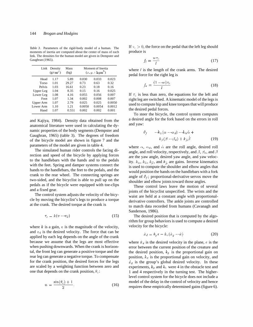
Table 3. Parameters of the rigid-body model of a human. Themoments of inertia are computed about the center of mass of eachlink. The densities for the human model are given in Dempster andGaughran (1965).

Link Density Mass Moment of Inertia(g/cm3) (kg) (x; y; z kgm2)

Head 1.17 5.89 0.030 0.033 0.023Torso 1.01 29.27 0.73 0.63 0.32Pelvis 1.03 16.61 0.23 0.18 0.16

Upper Leg 1.04 8.35 0.15 0.16 0.025Lower Leg 1.08 4.16 0.055 0.056 0.007

Foot 1.07 1.34 0.002 0.008 0.007Upper Arm 1.07 2.79 0.025 0.025 0.0050Lower Arm 1.10 1.21 0.0050 0.0054 0.0012

Hand 1.07 0.551 0.002 0.002 0.001

and Kajiya, 1984). Density data obtained from theanatomical literature were used in calculating the dy-namic properties of the body segments (Dempster andGaughran, 1965) (table 3). The degrees of freedomof the bicycle model are shown in figure 7 and theparameters of the model are given in table 4.

The simulated human rider controls the facing di-rection and speed of the bicycle by applying forcesto the handlebars with the hands and to the pedalswith the feet. Spring and damper systems connect thehands to the handlebars, the feet to the pedals, and thecrank to the rear wheel. The connecting springs aretwo-sided, and the bicyclist is able to pull up on thepedals as if the bicycle were equipped with toe-clipsand a fixed gear.

The control system adjusts the velocity of the bicy-cle by moving the bicyclist’s legs to produce a torqueat the crank. The desired torque at the crank is

�c = k(v � vd) (15)

where k is a gain, v is the magnitude of the velocity,and vd is the desired velocity. The force that can beapplied by each leg depends on the angle of the crankbecause we assume that the legs are most effectivewhen pushing downwards. When the crank is horizon-tal, the front leg can generate a positive torque and therear leg can generate a negative torque. To compensatefor the crank position, the desired forces for the legsare scaled by a weighting function between zero andone that depends on the crank position, �c:

w =sin(�c) + 1

2: (16)

If �c > 0, the force on the pedal that the left leg shouldproduce is

fl =w�c

l(17)

where l is the length of the crank arms. The desiredpedal force for the right leg is

fr =(1�w)�c

l(18)

If �c is less than zero, the equations for the left andright leg are switched. A kinematic model of the legs isused to compute hip and knee torques that will producethe desired pedal forces.

To steer the bicycle, the control system computesa desired angle for the fork based on the errors in rolland yaw:

�f = �k�(�� d) � k _� _�+

k�(� � �d) + k _�_� (19)

where �, �d, and _� are the roll angle, desired rollangle, and roll velocity, respectively, and �, �d, and _�

are the yaw angle, desired yaw angle, and yaw veloc-ity. k�, k _�, k�, and k _� are gains. Inverse kinematicsis used to compute the shoulder and elbow angles thatwould position the hands on the handlebars with a forkangle of �f ; proportional-derivative servos move theshoulder and elbow joints toward those angles.

These control laws leave the motion of severaljoints of the bicyclist unspecified. The wrists and thewaist are held at a constant angle with proportional-derivative controllers. The ankle joints are controlledto match data recorded from humans (Cavanagh andSanderson, 1986).

The desired position that is computed by the algo-rithm for group behaviors is used to compute a desiredvelocity for the bicycle:

_xd = kpe+ kv( _xg � _x) (20)

where _xd is the desired velocity in the plane, e is theerror between the current position of the creature andthe desired position, kp is the proportional gain onposition, kv is the proportional gain on velocity, and_xg is the group’s global desired velocity. In theseexperiments, kp and kv were 4 in the obstacle test and1 and 4 respectively in the turning test. The higher-level control system for the bicycle does not include amodel of the delay in the control of velocity and hencerequires these empirically determined gains (figure 6).


Table 4. The distance from the center of mass of each link to the distal and proximal joints in x, y, and z. A positive distance along the y axisrefers to a location on the left side of the body; a negative distance refers to the right side. The z axis is vertical and the x axis is positive in thedirection that the model is facing.

Link COM to Proximal COM to Distal(x; y; z m) (x; y; z m)

Torso to neck 0.012 0.0 0.32Torso to waist 0.012 0.0 -0.22

Torso to shoulder -0.048 �0.164 0.12Head -0.009 0.0 -0.064

Pelvis 0.023 0.0 0.103Pelvis to hips 0.005 �0.098 -0.11

Pelvis to bike seat 0.0 0.0 -0.15Upper Leg 0.024 �0.006 0.120 -0.05 �0.019 -0.21Lower Leg 0.005 �0.019 0.165 -0.002 �0.009 -0.25

Foot -0.046 �0.009 0.048Upper Arm -0.0002 �0.056 0.120 -0.005 �0.036 -0.17Lower Arm -0.025 �0.007 0.090 0.012 �0.014 -0.11

Hand -0.026 0.0 0.085Frame to bike seat -0.15 0.0 0.028

Frame to rear wheel -0.42 0.0 -0.36Frame to fork 0.46 0.0 0.09

Frame to crank 0.022 0.0 -0.36Fork to front wheel -0.026 0.0 0.085

Fork -0.05 0.0 0.108

Z

X

Y

Wrist−2DX

Shoulder−3D

X

Waist−3D

X Z

Z

Z

Waist−3D

Shoulder−3D

Elbow−1D

Y

Ankle−1DY

Hip−1D

Neck−1D

Y

Knee−1D

Y

Y

Y

YZ

Y

Crank−1D

Y

Wheel−1D

Fork−1D

Wheel−1DY

Z

X

Y

Fig. 7. The controlled degrees of freedom of the bicycle and human models. The human model has fourteen joints; the degrees of freedom ateach joint are shown in the diagram as are the four degrees of freedom of the bicycle model. The human rider is attached to the bicycle by apivot joint between the seat and the pelvis. The polygonal models were purchased from Viewpoint Datalabs.

4.3. Point-mass Simulation

The point masses have a mass equal to that of the

one-legged robots. The desired position computed by

the algorithm for group behaviors is used to compute

a force that is applied to the point mass:

f = kpe+ kv( _xg � _x) (21)

where kp and kv are gains, e is the error in position, _xis the velocity of the point mass and _xg is the globaldesired velocity. In these experiments kp was 6000and kv was 2000. There are no limits on the velocity.The point-mass system differs from the robots and


One-legged Robots

Point-mass Systems

Bicyclists

Fig. 8. The top two rows of graphs show the group of robots and the point-mass systems at a start state and every 7 s thereafter with a globaldesired velocity of 2.0 m/s. The bottom row of graphs shows the 18 bicyclists at a start state and every 20 s thereafter while they are riding at7.5 m/s. In each of these graphs the number of visible creatures, n, was set equal to the total number of creatures. Each point on the graphsrepresents the x and y position of an individual in the group. As a measure of the convergence to steady state, we computed the ratio of the xdimension to the y dimension of the bounding box around each group. A circular formation would have a ratio of 1. One-legged robots: 0.78,0.78, 0.93, 0.97 (for 0, 7, 14, 21 s). Point masses: 0.78, 0.98, 0.99, 0.99 (for 0, 7, 14, 21 s). Bicyclists: 1.33, 1.96, 1.56, 1.27 (for 0, 20, 40, 60 s).

bicyclists in that only the inertia of the mass preventsa given point mass from reaching its new desiredlocation within a single time-step.

5. Results

We tested the algorithm on three maneuvers: steady-state movement, turning, and avoiding obstacles. Forsteady-state movement, the initial configuration of theone-legged robots, the point masses, and the bicyclistswas a grid. The size of the groups of robots and pointmasses were the same (105) as were the initial veloc-ities of the individuals in the groups (2.0 m/s). Thegroup of bicyclists differed in that it had fewer mem-bers (18) and the initial velocity was higher (7.5 m/s).In our experiments, we considered systems to haveformed a circle when the ratio of the x dimension tothe y dimension of the bounding box surrounding thegroup was between 0.95 and 1.05. Once groups formed

a circle, there was very little change in the dimensionsof the bounding box and steady state was achieved.Due to the minimal dynamics present in the point-mass system, the group of point masses reached steadystate in under 7 s while the one-legged robots requiredslightly more than 14 s to reach steady state (figure 8).After 60 s, the group of bicyclists formed an ellipsoidalshape that was slowly becoming more circular. In thisexperiment, the number of visible creatures, n, wasset to equal the total number of creatures in the group.These circular shapes reflect the effects of the groupbehavior: each individual desires to be a specifieddistance from all visible neighbors. When this simplebehavior is aggregated over all members of a group,a regular group formation results that approximates acircle.

To navigate and accomplish tasks in a complexenvironment, creatures must not only be able to formgroups but they must also be able to turn and to avoidobstacles without collisions between the members of


One-legged Robots Point-mass Systems

0

10

20

30

40

50

y po

sitio

n (m

)

0 20 40 60 80 100

x position (m)

0

20

40

60

y po

sitio

n (m

)

0 20 40 60 80 100

x position (m)

Bicyclists

-20

0

20

40

60

y po

sitio

n (m

)

100 200 300 400

x position (m)

Fig. 9. The robots and point masses started in steady state at 2.0 m/s before the global velocity was changed to cause a 45 deg turn to the left.After 20 s the global desired velocity was turned 90 deg to the right. The bicyclists could not follow this path and required smaller turns. Thebicyclists started in steady state at 7.5 m/s before turning 22.5 deg to the left. After 20 s the global desired velocity was changed to turn 45 degto the right. Snapshots of the group formations were taken every 20 s and the path of one individual in the group is traced through the wholeturn.

the group. The second test of the algorithm involvedseveral turns. Beginning with a steady-state run, theglobal desired velocity was set first to cause a turn tothe left by 45 degrees and then after 20 s to cause aturn to the right by 90 degrees (figure 9).

The bicyclists could not turn as sharply as the robotsand point masses. As a result, the left turn for the bicy-clists involved a 10 s period where the global desiredvelocity changed gradually followed by a 10 s periodof constant desired velocity. The right turn was imple-mented in a similar fashion. The desired turning anglefor the bicyclists was half that of the points and robots.In these tests, all three systems completed the pathwithout collisions. The desired separation distance,D, was 5.0 m for the robots and point-mass systemsand 3.5 m for the bicyclists. When D was smaller, therobots had collisions near the point in time when theglobal desired velocity was changed. The number ofvisible neighbors, n, was set to 30 for the robots andpoint-mass systems and to 9 for the bicyclists.

To test whether the higher-level algorithm wouldallow the groups to navigate a course with obstacles,we positioned an obstacle in front of each type ofgroup when its members were moving in steady state.The values of n and D were the same as the turningtest. The robots and the point masses were allowed to

perceive the obstacle 5 m before they reached it; thebicyclists detected the obstacle when it was 13 m fromthe leading edge of the group. Because the bicyclistswere traveling at 7.5 m/s and the robots were runningat 2 m/s, both groups had approximately the samelength of time in which to react to the obstacle. Thegroup of point masses was able to avoid the obstacleand quickly rejoined to form a single group on the farside of the obstacle (figure 11). Both the robots andthe bicyclists were able to avoid the obstacle but wereslower to rejoin and form a single group (figure 10).

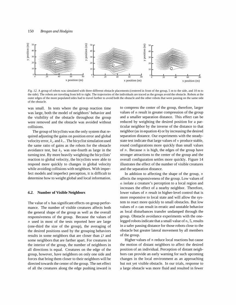
We used additional tests of obstacle avoidance toexplore further the performance of the algorithm forgrouping behaviors. The first set of tests containedthree trials which varied the position of the obstacleso that it was not centered in front of the group ofone-legged robots (figure 12). All three trials werecompleted without collisions. To permit the group toavoid the off-center obstacle without collisions, theamount of space allowed for each neighbor in the rect-angle between the individual and the obstacle (Doff )had to be doubled (figure 4).

A second set of trials tested the effect of varyingthe size of the group. An obstacle was centered infront of groups of 20, 40, 60, and 80 one-legged robots(figure 13). In these trials the leading edge of the


Fig. 10. Five pictures of the robots and the bicyclists as they avoid an obstacle.


One-legged Robots Point-mass Systems

0

10

20

30

40

y po

sitio

n (m

)

0 20 40 60 80

x position (m)

0

10

20

30

40

y po

sitio

n (m

)

0 20 40 60 80

x position (m)

Bicyclists

0

5

10

15

y po

sitio

n (m

)

0 20 40 60 80

x position (m)

Fig. 11. The trajectories of the individual robots, bicyclists, and point masses as the groups avoid an obstacle. The groups were moving left toright. In the case of the one-legged robots and the point-mass systems, the front edge of the group was positioned 5 m from the obstacle withan initial velocity of 2 m/s. The front edge of the bicyclists was positioned 13 m from the obstacle with an initial velocity of 7.5 m/s. In eachinstance, the radius of the obstacle was 2.0 m.

robot group was 10 m from the center of the obstacle.The number of visible neighbors, n, and the desiredseparation distance, D, were scaled proportionally forthe number of creatures in the group: n = 6, 13, 20,25 and D = 3, 4, 4.5, 5 m for groups of 20, 40, 60, and80, respectively. The four sizes of robot groups wereable to navigate past the obstacle without collisions.

6. Discussion

The algorithms for group behaviors used for these trialswere similar for the three systems and most differencesin performance can be attributed to differences in theunderlying dynamics and control. The group of pointmasses moved more tightly under changes in mag-nitude and direction of velocity because of the moreexact control of velocity. The robot group had morevariability and motion within the group, and the sep-aration distance was made larger to prevent collisionsbetween members. The control system for the bicy-clists was not as robust, and the bicyclists were notable to perform as well on the turning test. In moredifficult tests than those reported here, an individual in

the group of robots or bicyclists sometimes lost its bal-ance and fell. A maximum acceleration was enforcedfor the bicyclists and the robots to prevent limitationsin the low-level control from causing many of thesefailures. The point-mass systems had no notion ofbalance or maximum speed and could not fail in thisway.

6.1. Global and Local Communication

Communication as a means of coordination is implicitin the global desired velocity, _xg. In the turning test,forexample, a synchronous change in direction is causedby changing this global desired velocity. Reactionson a local scale, however, require local knowledge inaddition to global state information. This knowledgeis obtained by observing the positions and velocitiesof the n nearest neighbors. In the obstacle test, forexample, the position of the obstacle is known by allcreatures, but local information about the positionsof other creatures and a model of their behavior wasrequired to eliminate collisions when the reaction time


0

10

20

30

40

50

y po

sitio

n (m

)

0 20 40 60 80

x position (m)

0

10

20

30

40

50

y po

sitio

n (m

)

0 20 40 60 80

x position (m)

0

10

20

30

40

50

y po

sitio

n (m

)

0 20 40 60 80

x position (m)

Fig. 12. A group of robots was simulated with three different obstacle placements (centered in front of the group, 5 m to the side, and 10 m tothe side). The robots are traveling from left to right. The trajectories of the individuals are traced as the groups avoid the obstacle. Robots at theouter edges of the more populated sides had to travel farther to avoid both the obstacle and the other robots that were passing on the same sideof the obstacle.

was small. In tests where the group reaction timewas large, both the model of neighbors’ behavior andthe visibility of the obstacle throughout the groupwere removed and the obstacle was avoided withoutcollisions.

The group of bicyclists was the only system that re-quired adjusting the gains on position error and globalvelocity error, kp and kv. The bicyclist simulation usedthe same ratio of gains as the robots for the obstacleavoidance test, but kp was one-fourth as large in theturning test. By more heavily weighting the bicyclists’reaction to global velocity, the bicyclists were able torespond more quickly to changes in global velocitywhile avoiding collisions with neighbors. With imper-fect models and imperfect perception, it is difficult todetermine how to weight global and local information.

6.2. Number of Visible Neighbors

The value of n has significant effects on group perfor-mance. The number of visible creatures affects boththe general shape of the group as well as the overallresponsiveness of the group. Because the values ofn used in most of the tests reported here are large(one-third the size of the group), the averaging ofthe desired positions used by the grouping behaviorsresults in some neighbors that are closer than D andsome neighbors that are farther apart. For creatures inthe interior of the group, the number of neighbors inall directions is equal. Creatures on the edge of thegroup, however, have neighbors on only one side andforces that bring them closer to their neighbors will bedirected towards the center of the group. The net effectof all the creatures along the edge pushing inward is

to compress the center of the group, therefore, largervalues of n result in greater compression of the groupand a smaller separation distance. This effect can bereduced by weighting the desired position for a par-ticular neighbor by the inverse of the distance to thatneighbor (as in equation 4) or by increasing the desiredseparation distance. Our experiments with the steady-state test indicate that large values of n produce stable,round configurations more quickly than small valuesof n. Because n is high, the edges of the group havestronger attractions to the center of the group and theoverall configuration settles more quickly. Figure 14illustrates the effect of the number of visible creaturesand the separation distance.

In addition to affecting the shape of the group, naffects the responsiveness of the group. Low values ofn isolate a creature’s perception to a local region andincreases the effect of a nearby neighbor. Therefore,lower values of n result in higher-level control that ismore responsive to local state and will allow the sys-tem to react more quickly to small obstacles. But lowvalues of n can result in erratic and unstable behavioras local disturbances transfer undamped through thegroup. Obstacle avoidance experiments with the one-legged robots indicate that a small value ofn, 5, resultsin a safer passing distance for those robots close to theobstacle but greater lateral movement by all membersof the group.

Higher values of n reduce local reactions but causethe motion of distant neighbors to affect the desiredposition of an individual. Perception of distant neigh-bors can provide an early warning for such upcomingchanges in the local environment as an approachingbut not yet visible obstacle. In our trials, response toa large obstacle was more fluid and resulted in fewer


0

10

20

30

40

y po

sitio

n (m

)

0 20 40 60 80

x position (m)

0

10

20

30

40

y po

sitio

n (m

)

0 20 40 60 80

x position (m)

0

10

20

30

40

y po

sitio

n (m

)

0 20 40 60 80

x position (m)

0

10

20

30

40

y po

sitio

n (m

)

0 20 40 60 80

x position (m)

Fig. 13. Three groups of robots were simulated with a central obstacle location. The robots are traveling from left to right. The trajectoriesof the individuals are traced as the groups avoid the obstacle. The groups have 20, 40, 60, and 80 members, respectively. In each graph, theleading edge of the robots is placed 10 m from the center of the obstacle. The value of n has been scaled in proportion to the size of the group:n = 6, 13, 20, and 25 respectively. The desired separation distance has been scaled to maintain a consistent average separation distance betweenrobots: D = 3, 4, 4.5, 5 m.

n=6 D=2.5 n=30 D=2.5 n=105 D=3.5

Fig. 14. The first graph shows the initial configuration of robots for three experiments. The other three graphs show the configurations of thegroup after 80 s of simulation with each graph representing a different choice for the number of visible robots (n) and the desired separationdistance (D). When the robots were able to perceive a greater number of robots (n), the actual separation distance to the closest neighbors (d)was reduced even though the desired separation distance (D) to all visible robots increased. The actual average separation distance between anindividual and the set of neighbors in N was 2.36, 2.76, 4.78 m for the three trials. The average minimum separation distance between pairs ofcreatures was 1.98, 1.11, 0.95 m.

collisions when n was large. On the other hand, colli-sions may result if changes that occur only in the localenvironment are ignored because of the stability of themore distant environment.

Smaller values of nmay prevent a breakaway groupof sufficient size from joining another group becauseno individuals in the other group are visible to thosein the breakaway group. For the value of n used in

the obstacle test, the desired position relative to theobstacle had to be moved inward after the creaturewas safely past the obstacle to ensure that the twogroups always rejoined to form a single group. Inmore complex environments with many obstacles, thedecision to remain as separate groups or to join willbe more difficult. By increasing the complexity of theperception algorithm, creatures should have the ability


to distinguish nearby groups from more distant groupsthat can be ignored.

6.3. Limitations of the Grouping Behaviors

The algorithm for group behaviors that we imple-mented has several limitations. In some situations, theaveraging of desired positions moved two individualscloser to collision, and there is no reflexive reactionto an impending collision beyond the averaging ofdesired positions. We found that reflexive reactionscan create discontinuities in the calculation of the de-sired position that cause the dynamic simulations tobecome unstable. However, infrequent reflexive re-actions may avert some collisions and provide morerealistic-looking motion while maintaining the stabil-ity of the creature.

A second limitation is that our perceptual modelassumes more complete and accurate information thanthat produced by sensors on physical robots. We ex-perimented with other perceptual models by addingocclusion and reducing the visibility of creatures be-hind an individual as opposed to those in front. Whenthe set of visible creatures changes because of the ad-dition of a previously occluded individual, the desiredposition and velocity may change significantly, caus-ing a ripple effect throughout the group and increasingthe probability that an individual will lose its balance.

Although the robots and the bicyclists are dynamicsimulations, many factors are missing in the simula-tion that would be present in a physical system. Thesimulated motors do not have a maximum torque orlimited bandwidth, the joint and perceptual sensors donot have noise or delay, and the environment usedfor testing the algorithm for group behaviors does notcontain uneven or slippery terrain. The parameters forthe one-legged robot are similar to those of robots thathave been built (Raibert, 1986), but the parameters forthe bicyclist match those for a human and are superiorto the materials available for robot construction.

We have not explored the question of how the al-gorithm will perform on a heterogeneous population.Currently, each individual has the same dynamic prop-erties and control system. We plan, however, to varythe parameters for each individual to study the effectof a similar but nonhomogeneous population on theperformance of the algorithm.

Heterogeneous groups that mix types of simulatedcreatures could be studied by experimenting with low-speed, legged robots and higher-speed bicyclists inthe same environment. When tests such as obstacleavoidance and turning are performed on homogeneousgroups, the reaction of each individual is matchedby those of other members of the group becauseeach member has the same fundamental limitationsin low-level control. To work well, algorithms fornonhomogeneous groups must model these low-levellimitations in order to predict more accurately themotion of members of the group.

7. Acknowledgments

An earlier version of this paper appeared in the1995 IEEE/RSJ International Conference on Intelli-gent Robot and Systems. This project was sup-ported in part by NSF Grant Nos. IRI-9309189 andIRI-9457621, funding from the Advanced ResearchProjects Agency, and from Mitsubishi Electric Re-search Laboratory.

References

1. Arkin, R.C., 1992. Cooperation without Communication:Multi-agent Schema Based Robot Navigation. Journal ofRobotic Systems, Vol. 9(3), 351--364.

2. Arkin, R.C., and Hobbs, J.D., 1992. Dimensions of Com-munication and Social Organization in Multi-agent RoboticSystems. Proceedings of the Second International Conferenceon Simulation of Adaptive Behavior: From Animals to Animats2, 486--493.

3. Cavanagh, P., and Sanderson, D., 1986. The Biomechanics ofCycling: Studies of the Pedaling Mechanics of Elite PursuitRiders. Science of Cycling. E. Burke (ed), Chapter 5.

4. Cullen, J.M., Shaw, E., and Baldwin, H.A., 1965. Methods forMeasuring the Three-dimensional Structure of Fish Schools.Animal Behavior, 13:534--543.

5. Dempster, W.T., and Gaughran, G.R.L., 1965. Properties ofBody Segments Based on Size and Weight. American Journalof Anatomy, 120: 33--54.

6. Lien, S., and Kajiya, J. T. 1984. A Symbolic Method for Calcu-lating the Integral Properties of Arbitrary Nonconvex Polyhe-dra. IEEE Computer Graphics and Applications, 4(5):35--41.

7. Mataric, M., 1992a. Minimizing Complexity in Controllinga Mobile Robot Population. Proceedings of the 1992 IEEEInternational Conference on Robotics and Automation, 830--835.

8. Mataric, M., 1992b. Designing Emergent Behaviors: FromLocal Interactions to Collective Intelligence. Proceedings ofthe Second International Conference on Simulation of Adap-tive Behavior: From Animals to Animats 2, 432--441.

9. Mataric, M., 1993. Kin Recognition, Similarity, and GroupBehavior. Proceedings of the Fifteenth Annual Cognitive Sci-ence Society Conference, 705--710.


10. Parker, L.E., 1993. Designing Control Laws for CooperativeAgent Teams. Proceedings of the 1993 IEEE InternationalConference on Robotics and Automation, 582-587.

11. Raibert, M.H., 1986. Legged Robots That Balance. Cam-bridge: MIT Press.

12. Reynolds, C.W., 1987. Flocks, Herds, and Schools: A Dis-tributed Behavioral Model. Computer Graphics, 21(4): 25--34.

13. Rosenthal, D.E., and Sherman, M.A., 1986. High Perfor-mance Multibody Simulations via Symbolic Equation Manip-ulation and Kane’s Method.Journalof AstronauticalSciences,34(3):223--239.

14. Shaw, E., 1970. Schooling in Fishes: Critique and Review.Development and Evolution of Behavior. L. Aronson, E. To-bach, D. Leherman, and J. Rosenblatt (eds), W. H. Freeman:San Francisco, CA, 452--480.

15. Sugihara, K., and Suzuki, I., 1990. Distributed Motion Coor-dination of Multiple Mobile Robots. Proceedings of the 1990

IEEE International Conference on Robotics and Automation,138--143.

16. Takeuchi, R., Unuma, M., and Amakawa, K., 1992. PathPlanning and Its Application to Human Animation System.Computer Animation 1992, 163--175.

17. Wang, P.K.C., 1991. Navigation Strategies for Multiple Au-tonomous Robots Moving in Formation. Journal of RoboticSystems, 8(2):177--195.

18. Yeung, D.Y., and Bekey, G.A., 1987. A Decentralized Ap-proach to the Motion Planning Problem for Multiple MobileRobots. Proceedings of the 1987 IEEE International Confer-ence on Robotics and Automation, 1779--1784.

19. Veherencamp, S., 1987. Handbook of Behavioral Neurobi-ology, Volume 3: Social Behavior and Communication, P.Marler and J. G. Vandenbergh (eds.), Plenum Press: NewYork, NY, 354--382.

group behaviors for systems with signiﬁcant dynamicsdbrogan/publications/papers/jar_herd.pdf ·...

Documents