Svensk Kärnbränslehantering ABSwedish Nuclear Fueland Waste Management Co

Box 250, SE-101 24 Stockholm Phone +46 8 459 84 00

Ark

itekt

kopi

a A

B, B

rom

ma,

201

3

R-12-14

Groundwater flow modelling under ice sheet conditions in Greenland (phase II)

Olivier Jaquet, Rabah Namar, Pascal Siegel In2Earth Modelling Ltd

Peter Jansson Department of Physical Geography and Quaternary Geology, Stockholm University

November 2012

Tänd ett lager: P, R eller TR.

Groundwater flow modelling under ice sheet conditions in Greenland (phase II)

Olivier Jaquet, Rabah Namar, Pascal Siegel In2Earth Modelling Ltd

Peter Jansson Department of Physical Geography and Quaternary Geology, Stockholm University

November 2012

ISSN 1402-3091

SKB R-12-14

ID 1371241

Keywords: Geosphere model, Groundwater flow, Ice sheet, Permafrost, Taliks, Deformation zones, Glacial meltwater tracing.

This report concerns a study which was conducted for SKB. The conclusions and viewpoints presented in the report are those of the authors. SKB may draw modified conclusions, based on additional literature sources and/or expert opinions.

A pdf version of this document can be downloaded from www.skb.se.

SKB R-12-14 3

Contents

1 Introduction 5

2 Objectives 7

3 Conceptualisation 9

4 Phenomenology 114.1 Flow description 114.2 Permafrost description 114.3 Transport description 13

5 Geomodelling 155.1 Model domain 155.2 Topographic data and taliks 155.3 Deformation zones 175.4 The ice-bedrock boundary 18

5.4.1 Modelling subglacial thermal conditions 195.5 Hydraulic properties 225.6 Thermal and permafrost parameters 235.7 Transport parameters 235.8 Discretisation 245.9 Stochastic simulations 24

6 Modelling of groundwater flow and heat transfer 296.1 Reference case 30

6.1.1 Hydraulic boundary conditions 306.1.2 Simulation 32

6.2 Case 2 366.2.1 Boundary conditions 366.2.2 Simulation 36

6.3 Case 3 396.3.1 Boundary conditions 396.3.2 Simulation 40

6.4 Case 4 416.4.1 Boundary conditions 416.4.2 Simulation 41

6.5 Case 5 426.5.1 Boundary conditions 426.5.2 Simulation 43

7 Performance measures 457.1 Depth of permafrost 457.2 Tracing of glacial meltwater 46

7.2.1 Reference case 467.2.2 Case 2 487.2.3 Case 3 497.2.4 Case 4 507.2.5 Case 5 507.2.6 Concentration of glacial meltwater at 500 m depth 527.2.7 Concentration of glacial meltwater at taliks 54

8 Summary, conclusions, recommendations and perspectives 578.1 Depth of permafrost 578.2 Penetration depth and concentration of glacial meltwater 578.3 Concentration of glacial meltwater at taliks 588.4 Assumptions 58

4 SKB R-12-14

8.4.1 Conceptual assumptions 588.4.2 Data assumptions 598.4.3 Model assumptions 59

8.5 Sources of uncertainty 608.6 Future work 60

8.6.1 Integration of new GAP field data 608.6.2 Hydraulic properties 618.6.3 Permafrost characterisation 618.6.4 Transient boundary conditions 618.6.5 Phenomenology 61

References 63

SKB R-12-14 5

1 Introduction

To advance the understanding of the impact of glacial processes on the long-term performance of a deep geologic repository, the Greenland Analogue Project (GAP), a four-year field and modelling study of the Greenland ice sheet (2009–2012), was established collaboratively by the Swedish, Finnish and Canadian nuclear waste management organizations (SKB, POSIVA and NWMO, respectively). The Greenland ice sheet is considered to be an analogue of the conditions that could prevail in Canada and Fennoscandinavia during future glacial cycles. The funding organisations together with participation of researchers from universities and geological surveys in Canada, Denmark, Finland, Sweden, Switzerland, United Kingdom and the United States want to improve current understanding of continental ice sheet and permafrost effects on groundwater flow and water chemistry in crystalline rocks at depths resembling those of a potential deep geological repository for spent nuclear fuel.

SKB R-12-14 7

2 Objectives

The potential impact of long-term climate changes has to be evaluated with respect to repository performance and safety. In particular, glacial periods of advancing and retreating ice sheets and prolonged permafrost conditions are likely to occur over a repository site. The growth and decay of ice sheets and the associated distribution of permafrost will affect the chemical composition of the groundwater flow and its flow field. Since significant changes may take place, the understanding of groundwater flow patterns and composition during glaciations is an important safety issue for the geological disposal at long term. During a glacial period, the performance of the repository could be impacted by some of the following conditions and associated processes:

• Maximum pressure at repository depth (canister failure).• Maximum permafrost depth (canister failure, buffer function).• Darcy flux (buffer erosion).• Concentration of groundwater oxygen (canister corrosion).• Groundwater salinity and groundwater with low ionic concentrations (buffer stability).• Glacially induced earthquakes (canister failure).

Therefore, the GAP project aims at further understanding of key hydrogeological issues as well as answering specific questions:

• Regional groundwater flow system under ice sheet conditions.• Flow and infiltration conditions at the ice sheet bed.• Penetration depth of glacial meltwater into the bedrock.• Water chemical composition at repository depth in presence of glacial effects.• Role of the taliks, located in front of the ice sheet, likely to act as potential discharge zones

of deep groundwater flow.• Influence of permafrost distribution on the groundwater flow system in relation to build-up

and thawing periods.• Consequences of glacially induced earthquakes on the groundwater flow system.

Some answers are provided by the field data and investigations; the integration of the data, the dynamic characterisation and the understanding of the key processes is obtained through numerical modelling at regional scale. Preliminary scoping calculations were performed by developing a groundwater flow model under ice sheet conditions for the region of Kangerlussuaq (Jaquet et al. 2010). These calculations have highlighted the governing importance of specific factors, such as ice boundary conditions, permafrost and taliks on the groundwater flow system. Since new data and results become available, a second modelling phase is undertaken that aims at a more in depth understanding of groundwater flow conditions likely to occur underneath ice sheets. In particular, surface and basal glacial meltwater rates provided by a dynamic ice sheet model are assimilated into the groundwater flow model. In addition, the characterisation of the permafrost-depth distribution within the groundwater flow model is achieved using a coupled description of flow and heat transfer. Finally, the tracing of glacial meltwater produced by the ice sheet is modelled for the determination of depth and lateral extent likely reachable by glacial water.

This modelling approach which assimilates multiple data sources enables uncertainty reduction and consequently improves confidence when assessing selected measures for repository performance.

SKB R-12-14 9

3 Conceptualisation

The regional groundwater flow model under ice sheet conditions, the so-called geosphere model, is located in the SW part of Greenland near the town Kangerlussuaq (Figure 3-1). The geosphere model extends in an EW direction, roughly parallel to ice flow and hence, inferred general glacier hydrology flow direction.

In the region of Kangerlussuaq, between the coast and the ice sheet, the bedrock is dominated by banded gneisses which are frequently fractured and weathered. Amphibolites and pegmatitic dykes are associated with these extensively metamorphosed gneisses (Wallroth et al. 2010). Based on lineament interpretation and field observations, over a hundred major deformation zones and faults could be revealed for this region (Engström et al. 2012, Follin et al. 2011); these zones are likely more permeable than the surrounding metamorphic rocks. This geological medium with conductive deformation zones is considered as a 3D stochastic continuum; i.e. a continuum with stochastically described hydraulic properties.

The boundary conditions for the groundwater flow model are taken from an ice sheet model. These conditions are provided by the GAP ice sheet modelling group from the University of Montana. This group is developing and applying a 3D thermo-mechanically coupled ice sheet model (Rutt et al. 2009, CISM 2009) at the scale of the Greenland ice sheet. The thermomechanical ice model consti-tutes the core module where input for its boundary conditions are provided by: a) a climate driver for the upper surface temperature and mass balance fields, b) an isostasy model for the lower surface elevation and c) a geothermal model for the geothermal heat flux through the lower ice surface.

Figure 3-1. Geography of Greenland (left; after http://wwp.greenwichmeantime.com/time-zone/north-america/greenland/map/index.htm) and location of the geosphere model in relation to the Greenland digital bed elevation model (right; after Bamber 2001).

10 SKB R-12-14

In terms of physics, the core module of the ice sheet model integrates ice sheet mechanics, basal slid-ing, thermodynamics and basal hydrology. For the mechanical part, the shallow ice approximation is applied; i.e. bedrock and ice surfaces slopes are assumed sufficiently small that the normal stress components can be neglected.

The movement of the ice sheet – involving glacial build-up and retreat – is not taken into account for this modelling phase, the ice sheet conditions are considered in quasi-equilibrium at the investi-gated location. The state of the Greenland ice sheet is still not well understood. Krabill et al. (2000) showed that the interior of the ice sheet thickened while peripheral parts experienced thinning. That the Greenland ice sheet is experiencing losses have also been reported from GRACE data by Chen et al. (2006), Luthcke et al. (2006), Ramillien et al. (2006), and Velicogna and Wahr (2006). The results provide a strong independent indication that mass losses from the Southern part of Greenland ice sheet has increased substantially, thus verifying more local studies from Rignot et al. (1997), Howat et al. (2005), Rignot and Kanagaratnam (2006), and Luckman et al. (2006). Much of the mass losses observed are thus from dynamic response at outlet glaciers.

Since the geosphere model is more than 100 km away from the ocean, its influence is neglected; i.e. there are no fluctuations in ocean level as well as no supply of salt from the Davis Strait. Density-driven flow as induced by the variable salinity of the groundwater is not taken into account in the current modelling phase; it will be part of the third modelling phase. In addition, the impact of the ice sheet loading in terms of rock deformation leading to variations in porosity, hydraulic conductiv-ity and pore pressure is not included in the present modelling approach.

Therefore, the groundwater flow system is considered under steady state conditions and governed by infiltration of glacial meltwater in heterogeneous faulted crystalline rocks in the presence of permafrost (Figure 3-2). Two types of water are distinguished: glacial meltwater produced by the ice sheet and groundwater circulating at depth.

The permafrost is continuous in the periglacial environment, except at the location of taliks. Beneath the ice sheet, some permafrost regions of limited extent can still occur.

The depth variability of the permafrost depends on: 1) the surface and ground thermal steady state conditions, 2) the groundwater flow system, and 3) the geothermal flux from the Earth interior (Vidstrand 2003, Hartikainen et al. 2010). Permafrost is estimated to be approximately 335 m thick in this region, based on results from borehole DH-GAP03, drilled a few hundreds of meters away from the ice margin in summer 2009 (SKB 2010, Harper et al. 2011). In addition, first results from the deep research borehole DH-GAP04 that extends beneath the ice sheet, drilled during summer 2011, have shown values between 330–340 m for the permafrost thickness (Ruskeeniemi 2011, personal communication).

Figure 3-2. Simplified conceptual model for the groundwater flow system under ice sheet conditions, with talik (i.e. permafrost free area under the lake) and permafrost (in dark grey).

SKB R-12-14 11

4 Phenomenology

4.1 Flow descriptionFor the domain of the geosphere model, considered as a stochastic continuum, the calculation of groundwater flow under steady state conditions is obtained using the mass conservation equation (Svensson et al. 2010):

Q=zw+

yv+

xu

∂∂

∂∂

∂∂ρ (4-1)

where:

ρ fluid densityu, v, w Darcy velocitiesQ source/sink term.

The pressure equation is governed by Darcy’s law:

xP

gK=u x

∂∂−ρ

yP

gK

=v y

∂∂−ρ (4-2)

zP

gK=w z

∂∂−ρ

where:

Kx , Ky , Kz local hydraulic conductivities in x, y and z directionsg gravity accelerationP dynamic fluid pressure; P = p + ρ g z, with p the (total) pressure.

4.2 Permafrost descriptionThe modelling of permafrost-depth distribution requires the description of heat transfer coupled with groundwater flow. The formulation under steady state conditions of Ferry (Ferry M 2008. DarcyTools – Ice model, TR-08032, MFDRC. Unpublished report) is adopted which implies neglecting the temporal terms, among them the latent heat one. In addition, its contribution of water freezing to heath transfer is minor when porosity for water-saturated rocks is less than 1% (SKB 2006). The use of steady-state conditions for heat transfer is assumed a valid approximation considering the similar type of regime adopted for the flow boundary conditions underneath the ice sheet (cf. Section 6.1):

∂∂

∂∂

∂∂

∂∂−

∂∂

∂∂−

∂∂

∂∂−

∂∂ (4-3)

where:

T temperaturecp mass-specific heat capacity of fluidλx , λy , λz normal terms of equivalent thermal conductivity (i.e. rock + fluid) tensorQT source/sink term.

12 SKB R-12-14

According to the modelling approach applied at Laxemar (Vidstrand et al. 2010), no dependence is assumed between the dynamic viscosity of water and the temperature. The proportion of ice in the pore space is obtained using the following function (Figure 4-1):

−

−−

2LL

maxW

T)T(T,min

e1ic=ic (4-4)

where:

ic proportion of ice icmax maximum proportion of ice (set to 1)TL freezing temperatureW temperature interval for freezing.

The following reduction in hydraulic conductivity is applied for the permafrost (Figure 4-1):

:with

{ }15ref 10,Kmax=K −

( ){ }amin ic1,max −= αα

α (4-5)

where:

α reduction factorαmin lower bound for reduction factor (i.e. maximum reduction for permeability)a constant related to rock typeKref hydraulic conductivity of unfrozen rock.

And, the kinematic porosity of the frozen rock (permafrost) is obtained as follows:

ϕ = (1–ic) ϕref (4-6)

where:

ϕref kinematic porosity of unfrozen rock.

Figure 4-1. Ice content and log(hydraulic conductivity) curves as function of temperature.

SKB R-12-14 13

4.3 Transport descriptionThe tracing of glacial meltwater produced by the ice sheet is performed using the following transport equation (Svensson et al. 2010):

mwCmw

mwemw

mwemw

mwemw

mw

Q+CQ=zCDwC

z+

yCDvC

y+

xCDuC

x+

tC

∂∂−

∂∂

∂

∂−∂∂

∂∂−

∂∂

∂∂φρ (4-7)

where:

Cmv transported mass fraction of meltwaterDe effective diffusion coefficientQCmv source/sink term.

The application of eq. (4-7) assumes that the description of the medium heterogeneity in terms of a stochastic continuum enables the characterisation of the spatial variability for the fluid velocity and therefore captures the effects of kinematic dispersion. The effects of matrix diffusion were not considered in the present modelling phase.

Since our flow system is likely dominated by advective flow, the hybrid numerical scheme (Svensson et al. 2010) applied for solving the transport equation in DarcyTools should likely provided numerical dispersion effects with less than 2–3 grid cells of extension.

SKB R-12-14 15

5 Geomodelling

5.1 Model domainThe longest dimension of the 3D domain for the geosphere model extends about 150–200 km beneath the ice sheet and roughly 50 km in front of the ice sheet margin (Figure 5-1). The width of the model is approximately 60 km and its depth is set to about 5 km. The EW orientation of the domain, i.e. its long axis, coincides with the main ice flow direction. These dimensions are identical to those selected for the first modelling phase (Jaquet et al. 2010).

5.2 Topographic data and taliksThe applied topographic data are taken from the DEM data of Bamber (2001), Bamber et al. (2001) and Layberry and Bamber (2001). The data are available for bed elevation and ice thickness with a 5 km resolution for Greenland (Figure 5-2).

Figure 5-1. Location of the geosphere model with respect to the ice margin (red rectangle with an area of about 250 × 60 km2).

Figure 5-2. Greenland digital topographic data (Bamber 2001): bed elevation model (left) and ice thick-ness (right). The rectangle displays the location of the geosphere model.

16 SKB R-12-14

125 lakes were considered as potential taliks by SKB for the model domain located west of the ice margin. These potential taliks were selected on the basis of their size, i.e. a lake was considered as a potential talik if it had a size similar or larger than the Talik lake (i.e. the lake with approximate dimensions of 1,200 m × 400 m under which borehole DH-GAP01 is drilled).

The description of the perimeter of these taliks was obtained using LANDSAT satellite data (Figure 5-3). The surface elevation for the taliks was estimated by Aberystwyth University with the help of ASTER GDEM satellite data. The resulting elevation ranges from 52 to 710 m (Figure 5-4); the given vertical accuracy is 20 m at 95% confidence, at global scale (ASTER 2009).

Figure 5-3. Landsat image with talik location (light green), ice sheet and geosphere model boundary (red line).

Figure 5-4. Talik elevation: 52–200 m (black); 200–400 m (light blue); 400–600 m (green); 600–710 m (red), with ice margin in blue, and specific cross-cut location in red (X = 292, 310 and 345 km; Y = 931 km).

SKB R-12-14 17

5.3 Deformation zonesFor the description of the deformation zones, a geological model – called Geomodel version1 (Engström et al. 2012) – has been developed at regional scale and covers some area under the ice (Figure 5-5). This model integrates all topographical, geological and geophysical (aeromagnetic data from GEUS) information available, as well as the fracture data from the boreholes DH-GAP01 and DH-GAP03. Based on lineament interpretation supported by field observations, the Geomodel integrates a total of 158 potential deformation zones and faults (Figure 5-6) that were classified in four different sets. The Eastern area of the geosphere model is not covered by the Geomodel. Therefore, deformation zones and faults are duplicated towards the central part of the ice sheet, in order to introduce them in the geosphere model (Figure 5-7).

A talik is often a sign of a discharge area. These are generally found in topographic lows, which in turn often coincide where there is an outcropping deformation zone. Therefore, taliks are likely to be located on deformation zones. The obtained map shows that more than 75% of the taliks are associated to deformation zones (Figure 5-8).

Figure 5-5. Regional area of Geomodel version 1 (purple box) and GAP site scale area (red box), after Engström et al. (2012).

Figure 5-6. Geomodel version 1 map with four different types of deformation zones and faults: Type 1 = lilac (oldest), type 2 = green, type 3 = blue and type 4 = black (youngest). After Engström et al. (2012).

18 SKB R-12-14

5.4 The ice-bedrock boundaryThe ice bedrock interface conditions beneath the Greenland Ice Sheet are elusive, as they are under most glaciers and ice sheets. The interface condition has two major components, (1) whether or not the interface is at the melting point or sub-freezing and (2) whether the interface is a rock-ice contact or rock-sediment-ice contact. The first component determines whether liquid water can flow at the interface (melting conditions) or not whereas the other condition concerns whether or not water flow within a sediment aquifer can occur.

So far the basal temperature regime of the Greenland ice sheet has remained largely unknown. The geothermal heat flux exerts a strong control on basal temperatures (e.g. Waddington 1987). We know from Scandinavia that the geothermal heat fluxes vary substantially over shorter distances (Näslund et al. 2005). Hence the basal temperature is also likely to vary beneath the Greenland ice sheet. In addition to geothermal heat flux, internal and basal heat is generated from strain heating (e.g. Budd 1969, Table 4.2b, p. 69) and basal friction (e.g. Hooke 2005). These heat sources are coupled to ice dynamics which in turn can be coupled to melting conditions through feedback. Actual observations of basal temperature are lacking although indirect observations exist but are in some circumstances circumstantial.

Basal temperature has been calculated from measured temperature profiles in the deep boreholes through the Greenland ice sheet. Dahl-Jensen et al. (2003) used a combination of measurements

Figure 5-7. Geosphere model area (black box) with ice margin and duplicated deformation zones and faults taken from Geomodel version 1.

Figure 5-8. Location of deformation zones (red) and taliks (black), west of the ice margin (blue).

SKB R-12-14 19

and a flow line model to calculate heat flow variations along a flow line at NorthGRIP which yielded possibility to melt between 7.5–11 m a–1. Fahnestock et al. (2001) used an age-depth relationship from internal layering in the ice sheet to show that basal melting had occurred, exceeding 100 mm a–1 in one area. The basal conditions at the boreholes in these studies confirm the interpretations. In an air-borne campaign in Northern Greenland, Oswald and Gogineni (2008) used radio-echo intensity to map occurrence of subglacial water beneath the ice sheet. They could show that significant portions of the bed could be interpreted as melting. Their measurements do unfortunately not support an interpretation of what fraction of the bed is at melting conditions. The use of bed reflectivity as an indicator of melt-ing conditions has, however, been questioned by Matsuoka (2011). A further source for information is satellite magnetic measurements such as those interpreted by Fox Maule et al. (2005). Their data does not, however, provide good detail of the possible geothermal heat fluxes and hence does not allow us to interpret other than regional variability. Hence our understanding of basal thermal regime from measurements remains sketchy and in some instances uncertain and most often unknown.

Ice sheet modelling allows us to understand how the basal temperature can be affected by various effects such as geothermal heat fluxes (Näslund et al. 2005), ice dynamics and basal topography (van der Veen et al. 2007). Studies by Huybrechts (1995) and Marshall (2005) on the one hand, and Greve (2005) on the other, yield results that differ substantially. The former two studies yielded frozen condition beneath most of the ice sheet, thus contradicting observations, whereas the latter, while considering the measured temperatures as references in the model, yielded largely melting conditions. We are clearly far away from being able to provide a valid basal model of the ice sheet.

The occurrence of sediment beneath the ice sheet is also largely unknown. The spatial variability prob-ably occurs on all scales and may depend on topography. The central parts of the ice sheet are more likely to have continuous of semi-continuous sediment cover than the peripheral parts. In the periph-eral parts sediment cover will likely be distributed according to flow conditions. The proglacial area of the ice sheet does not exhibit thick covers over the bedrock highs and it is possible that this may also be true beneath the ice sheet. In the modern proglacial landscape the troughs are sediment filled but we must remember that this is largely due to proglacial postglacial deposition. Radar data (Harper J and Pettersson R 2011, personal communication) indicates that rapid flow features of the ice sheet in the Kangerlussuaq area is also associated with very deep troughs. It thus seems that sediment fills are not common to the troughs beneath the ice sheet. As a whole, the thickness and degree of patchiness of subglacial sediment covers remain largely unknown pending further analysis of geophysical data and further investigations.

5.4.1 Modelling subglacial thermal conditionsThe ice sheet covers a surface of about 200 × 60 km2, i.e. about 80% of the model domain. Beneath much of this area, regions of subglacial permafrost could likely occur. Due to this uncertainty, the impact of these regions on the flow system needs investigation. Therefore, a description of the subglacial thermal regime is needed for setting up a specific modelling case. A preliminary conceptual model was proposed by Pettersson (2011, personal communication) for the thermal regime underneath the ice sheet, based on the following dataset:

• LatestDEMresultsfromtheGAPprojectthatcharacterisesbedrocktopographyandicethicknesswith a 500 m resolution; these data covers a domain with an extension of about 100 km, east of the ice margin.

• IcevelocitythatwasmappedusingRADARSATsyntheticapertureradardata,availableatareso-lution of about 550 m. These data were processed by Aberystwyth University in order to overlay the entire domain of the geosphere model (Figure 5-9).

In the conceptual model of Pettersson (2011, personal communication), the location of subglacial melting (warm based) conditions is based on the following three criteria (Figure 5-10): ice velocity > 75 m/a, bed elevation < 300 m and ice thickness > 500 m. When these criteria are not met, sub glacial frozen (cold based) conditions are assumed to occur within the domain considered.

Since the entire geosphere model domain is not covered by the model of Pettersson (2011, personal communication), a stochastic model is required in order to characterise the Eastern and Northern parts of the domain. This model is founded on two datasets: the RADARSAT ice velocity (cf. Figure 5-9) and the Bamber DEM (Figure 5-11), both available at the scale of the geosphere model domain.

20 SKB R-12-14

The aim is to construct a model that captures the main characteristics of the model by Pettersson (2011, personal communication) (cf. Figure 5-10) and assimilate ice velocity and bed elevation datasets. Using this model, the distribution of subglacial thermal conditions is simulated for the entire domain of the geosphere model.

Figure 5-9. Ice velocity mapped on the geosphere model domain using RADARSAT data from winters 2000/01 and 2005/06 (Joughin et al. 2010). Acquisition is performed during winter periods for investigat-ing long-term change in ice velocity rather than summer variability affected by meltwater input.

Figure 5-10. Pettersson conceptual model for the subglacial thermal regime located solely in the Western part of the ice sheet. The red rectangle corresponds to the geosphere model domain.

Figure 5-11. Subglacial bed elevation after Bamber (2001) interpolated onto regular 500 m grid spacing.

SKB R-12-14 21

The spatial distribution of the subglacial thermal conditions is described using a random set model P obtained by thresholding a random function F at a given level (Figure 5-12). The idea is to first simulate a Gaussian random function correlated to the ice velocity and bed elevation datasets:

YYYF FZFVZ

FZV

FV221 ρρρρ −−+= (5-1)

where:

F Gaussian random function related to subglacial thermal conditionsρFV coefficient of correlation between subglacial thermal conditions and ice velocityYV Gaussian random function describing ice velocityρFZ coefficient of correlation between subglacial thermal conditions and bed elevationYZ Gaussian random function describing bed elevationY Gaussian random function.

Then, the spatial distribution of subglacial thermal conditions is obtained as follows:

Pλ = {F ≥ λ} (5-2)

where:

Pλ random set describing subglacial thermal conditionsλ threshold.

For example, if a threshold of zero is considered; since F is Gaussian, all positive values constitute zones of subglacial frozen conditions; and the zones with negative values are zones that present melting conditions. Using thresholds, categorical variables (value of 1 belongs to subglacial frozen conditions; zero is outside) are constructed for the spatial characterisation of subglacial thermal conditions in relation to the ice velocity and bed elevation. The threshold is deduced using the following inversion:

λ = F–1 [psmc] (5-3)

where:

psmc proportion of subglacial melting conditions.

The parameters used for the stochastic simulation of subglacial thermal conditions for the geosphere model domain are given in Table 5-1.

Figure 5-12. Stochastic simulation of subglacial thermal conditions where light grey is frozen and dark grey is melting conditions.

22 SKB R-12-14

Table 5-1. Parameters of subglacial thermal conditions for stochastic simulation.

Variogram model

Anisotropic correlation scales [km]

ρFV [–]

ρFZ [–]

psmc

Spherical 60.8 E–W 29.4 N–S

–0.8 0.2 0.6

The characterisation of the spatial variability of subglacial thermal conditions is performed using the ice velocity data due to their better resolution. By performing variogram analysis, an anisotropic spherical model is fitted to the ice velocity data: the correlation scales – i.e. the dominant spectral wave lengths – at which spatial variability occurs, are estimated at about 60.8 km and 29.4 km in the E–W and N–S directions respectively. The use of a spherical model delivers subglacial thermal patterns with smoother boundaries in comparison to the exponential model applied in Jaquet et al. (2010) for the description of these patterns.

The values for the coefficients of correlation and the proportion of subglacial melting conditions were chosen in order to match visually the main spatial patterns of the model by Pettersson (2011, personal communication). A stronger (absolute) value for the coefficient of correlation is given to the ice velocity data due to the reason mentioned above; its negative value indicates that the higher the ice velocity, the less likely subglacial frozen conditions are to occur. For the bed elevation, the value for the correlation coefficient is positive, and then frozen conditions are in correlation with bed elevation.

The obtained simulation (cf. Figure 5-12) provides a regional description of thermal subglacial conditions under the current uncertainties, as more data becomes available, improvements could be performed; in particular, the simulation could be conditioned to reproduce field observations of melting conditions in ice marginal areas.

For the geosphere modelling, subglacial frozen conditions are assumed to match the location of subglacial permafrost up to some depth.

5.5 Hydraulic propertiesSince the database of the GAP site is under development and for ease of model inter-comparison between the different modelling groups, the hydraulic properties for the geosphere model were provided by Follin et al. (2011). Due to the structural similarity between Geomodel version 1 (cf. Section 5.3) and the Laxemar deformation zone model, the hydraulic properties for the rock domain and the deformation zones are taken from this site in Sweden. The rock domain is divided into five hydrogeological units for which statistical parameters are available (Table 5-2). Permafrost is consid-ered present west of the ice margin up to a depth of 400 m. The hydraulic conductivity is assumed to follow a log-normal distribution with an isotropic exponential variogram. The correlation scale is assumed to remain constant for the five hydrogeological units considered.

Table 5-2. Geosphere hydraulic properties for rock domain and permafrost according to the Laxemar site (after Follin et al. 2011).

Lithology Depth[m]

Geometric mean of hydraulic conductivity [m/s][log value] (scale of hydraulic test in m)

Standard deviation[log 10]

Correlation scale[m]

Permafrost1) 0–400 10–15 – –Crystalline 0–200 1.1·10–7 [–6.96] (100) 1.04 2752)

Crystalline 200–450 1.5·10–8 [–7.81] (100) 1.63 275Crystalline 450–700 8.9·10–10 [–9.05] (100) 1.78 275Crystalline 700–1,000 2.2·10–10 [–9.66] (100) 1.70 275Crystalline3) 1,000–5,000 2.2·10––10 [–9.66] 1.70 275

1) Distribution of permafrost. (a) Absent or discontinuous under the ice sheet (subglacial permafrost). (b) Elsewhere continuous except in presence of taliks.2) Corresponds to the range of the spherical isotropic variogram used by Rhén et al. (1997).3) Depth range with assumed values.

SKB R-12-14 23

The hydraulic tests at Laxemar were performed at 100 m scale. A change of scale is required for the attribution of the hydraulic conductivity at the cells of the numerical model. A simple additive correction is applied to the correlation scale; i.e. its value is extended to 775 m in relation to the cell size (500 m) used for numerical modelling (cf. Section 5.8). This correction delivers an upper value for the correlation scale, allowing parameter homogenisation at a 500 m scale. The variance of the hydraulic conductivity is assumed to remain unaffected by this change of scale.

The hydraulic properties for the deformation zones are also taken from the Laxemar site. The depth dependency of the in-plane transmissity for the deformation zones is described using an exponential model (Follin et al. 2011) expressed as:

( )

( ) ( )m1,000zTm1,000zT

10,10)0(Tmax=m1,000zT 9kz

−==−<

−≥ −

(5-4)

where:

T(z) transmissivity of deformation zoneT(0) transmissivity at zero elevationk depth interval giving one order magnitude of decrease in transmissivity; the values applied for

k ranges from 365.0–534.8 m (Follin et al. 2011).

5.6 Thermal and permafrost parametersThe thermal and permeability reduction parameter for the modelling of permafrost modelling are given in Tables 5-3 and 5-4; these parameter values correspond to the values taken for the Laxemar site (Vidstrand et al. 2010), except for the geothermal heat flux field taken from (Shapiro and Ritzwoller 2004).

Table 5-3. Thermal parameters.

Mass-specific heat capacity of fluid[J kg–1 °C–1]

Equivalent thermal conductivity (rock+fluid)[W m–1 °C–1]

Geothermal heat flux[W m–2]

4,182 2.75 Spatially variable

Table 5-4. Permeability reduction parameters.

TL

[°C]W[°C]

αmin [–]

A[–]

0 0.5 10–10 5

5.7 Transport parametersThe transport parameters used for glacial meltwater tracing are given in Table 5-5. The value for the molecular diffusion coefficient is taken from de Marsily (1981). The effective diffusion coefficient is equal to the product of the molecular diffusion coefficient by the mean (arithmetic) value of the kinematic porosity.

Table 5-5. Transport parameters.

Molecular diffusion coefficient [m2 s–1]

Mean (kinematic) porosity[–]

De

[m2 s–1]

10–9 3.6·10–4 3.6·10–13

24 SKB R-12-14

The kinematic porosity is calculated from the hydraulic conductivity using the following equation (Rhén et al. 1997; Follin et al. 2011):

ϕ = 34.87 K 0.753 with ϕ ≤ 0.05 (5-5)

5.8 DiscretisationThe discretisation is performed using an unstructured Cartesian grid system. The grid resolution is 500 m in the horizontal directions. The discretisation in the vertical direction varies between 25, 50 or 100 m when approaching the topographic surface. The model contains about 3,600,000 cells.

The elevation of the top surface of the model domain is estimated from DEM data (Bamber 2001, Bamber et al. 2001, Layberry and Bamber 2001), available at 5 km resolution for Greenland (cf. Section 5.2). In addition, all the potential taliks located west of the ice margin within the studied domain were discretised, in terms of geometry and elevation, for geosphere modelling (cf. Figure 5-4). Some of the taliks are regrouped with other ones, due to their small size.

The Bamber (bed) elevation results from an interpolation at 5 km resolution. These DEM data together with the talik elevation values, determined using satellite data (cf. Section 5-2), are inter-polated onto a regular grid with a spacing of 500 m (Figure 5-13). The use of these two datasets of different quality leads to some inconsistencies in the neighbourhood of some taliks; i.e. in the form of local topographic irregularities.

5.9 Stochastic simulationsHydraulic propertiesThe description of the spatial variability of the hydraulic conductivity is obtained at the cell scale of the rock domain by a stochastic simulation using the turning bands method (Matheron 1973, Lantuéjoul 2002). The details of the applied stochastic methodology are given in Jaquet et al. (2010). A Gaussian standard normalised simulation of the hydraulic conductivity logarithm is carried out using an isotropic exponential variogram with a correlation length of 775 m (cf. Section 5.5). Then, this simulation is scaled according to the mean and standard deviation of the hydraulic conductivity (cf. Table 5-2) given for the five hydrogeological units (Figure 5-14).

Figure 5-13. Interpolated elevation using Bamber (2001) and talik elevation data onto regular 500 m grid spacing. Taliks are displayed in thin black line and ice margin in thick black line (coordinates in km). Taliks at high elevation are not located on the top of hills; this effect is related to the coarse resolution of the DEM data.

SKB R-12-14 25

The simulation of the lateral in-plane variability of the deformation zone transmissivity (Follin et al. 2011) is obtained by adding a stochastic residual – without spatial correlation – to the exponential model (cf. eq. 5-4):

( )

( ) ( )m1,000zTm1,000zT

10,10)0(Tmax=m1,000zT 9Ykz

R

−==−<

−≥ −+

(5-6)

where:

YR log-residual with Gaussian distribution (mean = 0 and standard deviation = 1.35).

Using the above model (eq. 5-6), the range for hydraulic conductivity and porosity values of the deformation zones is displayed in Figure 5-15.

Figure 5-14. Stochastic simulation of log-conductivity field (purple represents permafrost with K = 10–15 m/s; gaps are related to taliks), W-E vertical cut at Y = 931 km (x-coordinate in km; z-coordinate in m/50).

Figure 5-15. Deformation zones: variability of hydraulic conductivity (above) and porosity (below) in relation to elevation.

26 SKB R-12-14

The deformation zones are integrated into the cells discretising the rock domain using the GEHYCO method (Svensson et al. 2010); i.e. for each cell face, the hydraulic conductivity is calculated to take into account the contribution of the intercepting deformation zones. Then, the joint effect of deformation zones and rock domain is considered by calculating equivalent hydraulic conductivities for each cell face, as follows (Figure 5-16):

{ }RDi

DZii K,Kmean=K (5-7)

where:

KiDZ hydraulic conductivity related to deformation zone(s) at face i (i = x, y or z)

KiRD hydraulic conductivity related to rock domain at face i (i = x, y or z).

The resulting stochastic simulation of hydraulic properties with the deformation zones is displayed in Figure 5-17.

PorosityThe porosity is calculated from the stochastic hydraulic conductivity field using eq. (5-5) for each cell centre.

PermafrostIn the reference case, no frozen conditions are present underneath the ice sheet. Since frozen conditions could occur, an alternative description is considered using a stochastic distribution for subglacial permafrost zones where their locations are correlated with regions of lower ice velocity as well with those of higher elevation (cf. Section 5.4).

CoarseningFinally, due to the variable vertical discretisation scheme (cf. Section 5.8) near the surface of the geosphere model, a coarsening is performed to the hydraulic properties (Figure 5-18); i.e. their variability is rendered independent of the cell size along the vertical direction, so that this variability always occurs at 100 m scale in order to respect the input statistical parameters (cf. Table 5-2).

Figure 5-16. Example of equivalent hydraulic conductivity for face x using KxDZ and Kx

RD, for the left cell intersected by a deformation zone.

SKB R-12-14 27

Figure 5-17. Stochastic simulation of log-conductivity field with deformation zones and ice margin (red), horizontal cut at z = –2,500 m (coordinates in km).

Figure 5-18. Coarsening principle: i.e. starting from the top, four 25 m size consecutive cells along the vertical direction present identical values (same colour) for their hydraulic properties. W-E vertical cut at Y = 931 km (x-coordinate in km; z-coordinate in m/100).

SKB R-12-14 29

6 Modelling of groundwater flow and heat transfer

Groundwater flow under ice sheet conditions is modelled for five different cases whereby the subglacial boundary conditions are provided by an ice sheet model (Figure 6-1). The first one is the reference case; case 2 is specifically dedicated to the assessment of the permafrost depth variability while accounting for heat transfer. The remaining cases consider boundary conditions and parameter sensitivity. The foreseen cases with their differences in terms of processes, permafrost and boundary conditions are given in Table 6-1. The applied parameters are defined in the preceding sections. Calculations were performed using the DarcyTools simulator, version 3.3.2 (Svensson et al. 2010). The steady-state system was solved with an order of time discretisation of 0 and using 300 sweeps, in order to reach convergence with a residual mean square error value equal to 10–9, for all of the cases.

Figure 6-1. Cartoons for case visualisation: case 1 (reference); case 2 with simulated permafrost; case 3 with LGM scenario; case 4 with prescribed pressure; case 5 with discontinuous permafrost under the ice.

30 SKB R-12-14

Table 6-1. Characteristics of the five modelling cases.

Case Processes Permafrost Boundary conditions west of ice margin

Boundary conditions under the ice sheet

Objectives

1 Flow Fixed depth: continuous west of ice margin except at taliks and absence under ice

Prescribed pressure in taliks and no-flow conditions elsewhere

Prescribed mean meltrate from ice sheet model (Scenario I)

Reference

2 Flow, heat Variable depth (calcu-lated): continuous west of ice margin except at taliks and discontinuous under ice

Prescribed pressure in taliks and no-flow conditions elsewhere

Prescribed mean meltrate from ice sheet modelPrescribed temperature from ice sheet model(Scenario I)

Sensitivity to permafrost depth

3 Flow Fixed depth: continuous west of ice margin except at taliks and absence under ice

Prescribed pressure in taliks and no-flow conditions elsewhere

Prescribed meltrate from ice sheet model(Scenario II)

Sensitivity to meltrate

4 Flow Fixed depth: continuous west of ice margin except at taliks and absence under ice

Prescribed pressure in taliks and elsewhere

Prescribed mean meltrate from ice sheet model(Scenario I)

Sensitivity to prescribed pres-sure west of ice margin

5 Flow Fixed depth: continuous west of ice margin except at taliks and discontinuous under ice

Prescribed pressure in taliks and no-flow conditions elsewhere

Prescribed mean meltrate from ice sheet model(Scenario I)

Sensitivity to permafrost under the ice

6.1 Reference caseFor the reference case, the permafrost is only located in front of the ice margin with the exception of the taliks (cf. Figure 5-14); its thickness is set to a constant value of 400 m, on the basis of the avail-able data (cf. Chapter 3). The boundary conditions applied for the reference case are defined below.

6.1.1 Hydraulic boundary conditionsIn relation to the ice margin and model geometry, the flow boundary conditions are as follows:

• Surface of the model (underneath the ice sheet): a spatially variable meltwater rate is applied, where the values are provided by an ice sheet simulation (Rutt et al. 2009, CISM 2009) repre-sentative of the present day conditions. The set up and runs for the ice sheet model were much the same as those applied by Greve et al. (2011). The total meltwater rate is estimated as follows:

TMR = 0.3 SMR + BMR (6-1)

where

TMR total meltwater rateSMR surface meltwater rate from the ice sheet simulation with a 5 km resolutionBMR basal meltwater rate from the ice sheet simulation with a 5 km resolution.

Since steady state conditions are considered, a weighting coefficient is applied to the surface melt-water rate, because it occurs only during the summer period. The total meltwater rate (Figure 6-2) is used as input to a mixed boundary condition; i.e. the prescribed flux equals the total meltwater rate expressed in terms of dynamic fluid pressure (cf. eq. 4-2) constrained by the ice thickness, as follows:

SKB R-12-14 31

qBC if PBC0 < PBC

ice else PBC = PBCice (6-2)

where:

qBC prescribed flux; i.e. total meltwater rate from the ice sheet modelPBC

0 computed dynamic fluid pressure at boundaryPBC

ice dynamic fluid pressure corresponding to the ice thickness contributionPBC prescribed dynamic fluid pressure.

With the dynamic fluid pressure, corresponding to the ice thickness contribution, written as:

zg+hcg=P watericeiceiceiceBC ρρ (6-3)

where:

ρice ice density (= 917 kg/m3)cice ice contribution coefficient (= 0.9)hice ice thickness (Figure 6-3)ñwater water densityz elevation.

The approach used for mixed boundary conditions (eq. 6-2) is similar to the one applied by Lemieux et al. (2008).

The formulation of eq. (6-3) means that the pressure contribution due to ice is equivalent to an ice column corresponding to the ice sheet thickness multiplied by an ice contribution coefficient. The ice thickness data from Bamber (2001) are the results from an interpolation at 5 km; it was then fol-lowed by a second interpolation of the ice thickness down to 500 m resolution to meet the modelling needs (cf. Figure 6-3). The consequence is that the ice thickness data used for modelling are associ-ated with large interpolation uncertainties. Therefore, in order to avoid potential overestimation of ice thickness leading to a (unrealistic) floating of the ice and consequently too strong gradients, it was decided, based on expert judgement, to choose a value equal to 0.9 for the ice contribution coefficient.

Figure 6-2. Total meltwater rate log[m/a] from ice sheet simulation for present day conditions interpolated onto regular 500 m grid spacing of the subglacial model domain.

32 SKB R-12-14

• Surface of the model (west of the ice margin): at talik location, a dynamic fluid pressure Ptalik = ρ g z is prescribed, where z will correspond to talik surface elevation. Outside of taliks, conditions of no-flow are prescribed for the topographic surface.

• Lateral west boundary of the model: a hydrostatic condition is prescribed with a dynamic fluid pressure equal to ρ g z, where the surface elevation z is set to 87.5 m. This value corresponds to the minimum elevation of the topography along the Western boundary; it was selected as to diminish the gradients likely to occur from the Western boundary towards a small number of the taliks with low elevation. Attempts with the average elevation value of the Western boundary lead to an unrealistic flow field and were therefore abandoned. Some uncertainty remains with this value selected for the Western boundary, as it is derived from a DEM with a 5 km resolution.

• Lateral north+south+east and bottom boundaries: no-flow conditions are currently pre-scribed. In presence of new information, such as the bed topography that will be provided by the analysis and interpretation of the GAP radar data, the type of these boundaries shall be modified accordingly.

6.1.2 SimulationFor the reference case, groundwater flow simulation is performed under steady state conditions (cf. Chapter 4). Regarding the mixed hydraulic boundary conditions beneath the ice sheet, an iterative procedure is needed; using the specified flux values (i.e. the total meltwater rate), the head solution is calculated at each iteration. After each iteration, the solution is analysed: if boundary value(s) with hydraulic head higher than the ice thickness occur, the iteration is restarted with prescribed hydraulic head – equal to the ice contribution, cf. eq. (6-2) – for these boundary values. After the convergence of the mixed boundary conditions, a final run with fixed boundary conditions is performed in order to improve convergence, in terms of lowering the value of the residual mean square error.

On the topographic surface, west of the ice margin, only taliks are open to flow, due to their prescribed pressure (cf. Section 6.1.1). The obtained results expressed in terms of hydraulic head (in meters) are shown along selected horizontal and vertical cuts orientated N-S and E-W (Figure 6-4).

The regional hydraulic gradient is controlled by the infiltration of meltwater provided by the ice sheet as displayed on Figure 6-5 and 6-6. Groundwater flow occurs regionally from east to west under the ice as well as west the ice margin. The Eastern part is dominated by a boundary condition of the pre-scribed flux type (Figure 6-7). Towards the ice margin, with the increase in glacial meltwater rates, prescribed pressure conditions related to the ice thickness govern groundwater flow (Figure 6-8). Locally, discharge conditions can occur underneath the ice sheet where pressure conditions are pre-scribed in relation to the variability of topography and ice thickness (Figures 6-7 and 6-8). When com-pared to previous modelling results (Jaquet et al. 2010), the meltwater rates provided by the ice sheet model produce a more realistic flow field in the Eastern part of the domain.

Figure 6-3. Ice thickness [m] (Bamber 2001) interpolated onto regular 500 m grid spacing of the subglacial model domain.

SKB R-12-14 33

Figure 6-4. Cross-cut location in green (X = 292, 310 and 345 km; Y = 931 km) with deformation zones (red), taliks (black) and ice margin (blue).

Figure 6-5. Reference case: hydraulic head [m], W–E vertical cut at Y = 931 km (x-coordinate in km; z-coordinate in m/50).

Figure 6-6. Reference case: hydraulic head [m], horizontal cut at Z = –62 m (coordinates in km).

34 SKB R-12-14

Figure 6-7. Reference case: boundary conditions (above); no-flow (grey), prescribed hydraulic head (colours) and prescribed flux (black) and corresponding hydraulic head on the subglacial model surface (below), (all coordinates in km).

Figure 6-8. Reference case: hydraulic head [m], S–N vertical cut at X = 345 km (y-coordinate in km; z-coordinate in m/100). The thickness of the ice sheet increases towards the south (cf. Figure 6-3).

SKB R-12-14 35

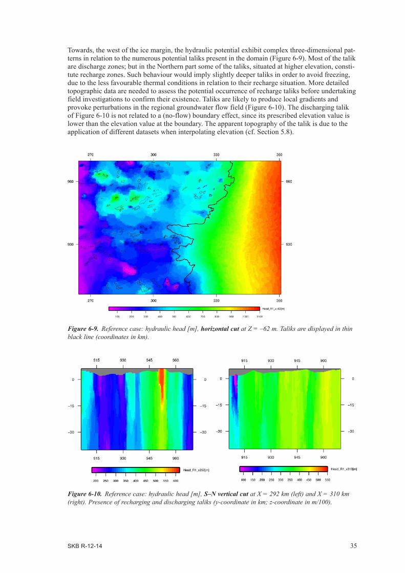
Towards, the west of the ice margin, the hydraulic potential exhibit complex three-dimensional pat-terns in relation to the numerous potential taliks present in the domain (Figure 6-9). Most of the talik are discharge zones; but in the Northern part some of the taliks, situated at higher elevation, consti-tute recharge zones. Such behaviour would imply slightly deeper taliks in order to avoid freezing, due to the less favourable thermal conditions in relation to their recharge situation. More detailed topographic data are needed to assess the potential occurrence of recharge taliks before undertaking field investigations to confirm their existence. Taliks are likely to produce local gradients and provoke perturbations in the regional groundwater flow field (Figure 6-10). The discharging talik of Figure 6-10 is not related to a (no-flow) boundary effect, since its prescribed elevation value is lower than the elevation value at the boundary. The apparent topography of the talik is due to the application of different datasets when interpolating elevation (cf. Section 5.8).

Figure 6-9. Reference case: hydraulic head [m], horizontal cut at Z = –62 m. Taliks are displayed in thin black line (coordinates in km).

Figure 6-10. Reference case: hydraulic head [m], S–N vertical cut at X = 292 km (left) and X = 310 km (right). Presence of recharging and discharging taliks (y-coordinate in km; z-coordinate in m/100).

36 SKB R-12-14

6.2 Case 2Case 2 is characterised by the modelling of the permafrost-depth distribution using groundwater flow and heat transfer calculations under steady state conditions (cf. Chapter 4). The presence of permafrost leads to a modification of the hydraulic conductivity and the porosity in relation to the ice content (cf. Chapter 4). The flow boundary conditions remain identical to the reference case.

6.2.1 Boundary conditionsIn addition to the flow boundary conditions (cf. Section 6.1.1), the following thermal boundary conditions are applied:

• Surface of the model (west of the ice margin): the mean annual air temperature for present day, given by the GAP ice sheet modelling group and derived from Fausto et al. (2009), is prescribed west of the ice margin (Figure 6-11). At talik locations, the prescribed temperature is set to 4°C (Claesson Liljedahl L 2010, personal communication, Vidstrand et al. 2010).

• Surface of the model (underneath the ice sheet): the prescribed temperature is set to 0.01°C for the subglacial domain, as melting conditions are indicated by the ice sheet simulation representa-tive of the present day conditions (Figure 6-12). The exception being the far NE corner of the domain where frozen conditions occur; the prescribed negative temperature values are taken from the ice sheet simulation. This small zone is of little relevance for the modelling; however, this frozen location is probably linked to the ice thickening occurring in the NE (cf. Figure 6-3).

• Bottom boundary: the distribution of geothermal heat flux (Figure 6-13) was inferred by Shapiro and Ritzwoller (2004). The developed method uses a global seismic model to guide the extrapolation of heat flow measurements to regions where direct measurements are rare. This method is stochastic and currently produces only average values that were applied as prescribed geothermal heat flux. At the bottom boundary, using a relationship given in Hartikainen et al. (2010), the decrease of surface heat flux is estimated to about 20%. Since the uncertainty associ-ated to the surface heat flux is much larger than the heat flux variability with depth; the latter is neglected and the surface heat flux is taken as bottom boundary condition.

6.2.2 SimulationFor case 2, a groundwater flow simulation coupled with heat transfer is performed under steady state conditions (cf. Chapter 4). In order to avoid convergence problems, the fixed distribution of mixed boundary conditions for the subglacial domain is taken from the reference case. Due to the size of the model, the numerical resolution of the flow and heat transfer equations is weakly coupled by linearising the equations. At each iteration, the simulation is carried out in two stages: (a) resolution of groundwater flow (b) resolution of heat transfer and modification of hydraulic properties accord-ing to the temperature field. This iterative procedure is stopped when the value for the criteria of convergence is reached during the simulation.

Figure 6-11. Case 2: mean annual air temperature [°C] for present day conditions interpolated onto regular 500 m grid spacing of the model domain (coordinates in km).

SKB R-12-14 37

The taliks remain open to flow, due to their positive prescribed temperature. But, in comparison to the reference case, the depth of the permafrost becomes variable; influenced by the tempera-ture field and the groundwater circulations (Figure 6-14). This result justifies the application of groundwater flow coupled with heat transfer. For case 2, the absence of coupling would have not lead to the depth variation observed for the permafrost.

Since mean annual air temperature is taken as input for permafrost simulation, surface cover effects (Hartikainen et al. 2010), such as vegetation and snow cover, likely to increase the ground temperature were neglected for this study. Due to the colder temperature applied as surface boundary condition west of the ice margin, the simulated depth distribution for the permafrost of case 2 can be considered as a conservative estimate.

At the base of the permafrost, a transition zone is present with a gradual reduction in hydraulic conductivity as function of the ice content (Figure 6-15). Such effects in addition to the depth vari-ability of permafrost lead to modifications of the hydraulic conductivity field near the surface, west of the ice margin. In consequence, local modifications of the flow system compared to the reference case (cf. Figure 6-10) are likely to occur; e.g. in the vicinity of taliks (Figure 6-16). The number and location of recharge taliks remains the same as the ones of the reference case; the same results were obtained for the other cases.

Figure 6-12. Case 2: subglacial thermal regime for present day conditions given by the ice sheet model interpolated onto regular 500 m grid spacing of the subglacial model domain, where dark grey is melting conditions and light grey is frozen conditions (coordinates in km).

Figure 6-13. Case 2: geothermal heat flux [W/m2] interpolated onto regular 500 m grid spacing of the model domain (coordinates in km).

38 SKB R-12-14

Figure 6-14. Case 2: simulation of permafrost depth-distribution (left: in purple) in comparison to the reference case (right) with fixed permafrost depth, W–E vertical cut at Y = 931 km (x-coordinate in km; z-coordinate in m/50).

Figure 6-15. Case 2: ice content [–], S–N vertical cut at X = 310 km (y-coordinate in km; z-coordinate in m/100).

SKB R-12-14 39

6.3 Case 3For case 3, an alternative glaciation scenario is considered as input to the geosphere model. It means that a different distribution for the meltwater rate is applied as subglacial boundary conditions.

6.3.1 Boundary conditionsIn comparison to the reference case, only the following flow boundary conditions differ:

• Surface of the model (underneath the ice sheet): as before, a spatially variable meltwater rate is applied provided by an ice sheet simulation (Rutt et al. 2009, CISM 2009), but representing conditions of the Last Glacial Maximum (LGM). This ice sheet simulation describes glaciation conditions that have occurred about 17’000 years ago in Greenland (Figure 6-17). Therefore, only basal meltwater rate are available and they are used as input to the mixed boundary conditions (cf. Section 6.1.1). The meltwater rate for the LGM scenario present lower values compared to the present day scenario (cf. Figure 6-2).

For the geosphere model domain, the ice thickness values obtained from the ice sheet simulation are problematic due to data assimilation issues; i.e. they are about one order of magnitude lower than the values from the Bamber (2001) dataset. Therefore, for case 3, it was decided to apply the LGM scenario with ice sheet thickness related to present day conditions (cf. Figure 6-3); i.e. to apply consistent estimates of ice thickness for the calculations of the subglacial boundary conditions.

Figure 6-16. Case 2: hydraulic head [m], S–N vertical cut at X = 292 km (left) and X = 310 km (right). Presence of discharging and recharging taliks (y-coordinate in km; z-coordinate in m/100).

Figure 6-17. Case 3: basal meltwater rate log[m/a] from ice sheet simulation for LGM conditions interpolated onto regular 500 m grid spacing of the subglacial model domain.

40 SKB R-12-14

6.3.2 SimulationAs for the preceding cases, a groundwater flow simulation is performed for case 3 under steady state conditions. Since alternative subglacial boundary conditions (LGM scenario) are applied, the iterative procedure for the mixed boundary conditions needs to be carried out again for case 3 (cf. Section 6.1.2). Most of the subglacial domain becomes dominated by boundary conditions of the flux type (Figure 6-18) due to the use of lower meltwater rate values in comparison to the reference case (cf. Figure 6-7). The rather geometric shape of the limit between prescribe head and infiltration boundary conditions is related to the patterns of the basal meltwater that increases toward the SW of the ice margin (cf. Figure 6-17).

The LGM scenario leads to a diminution of the EW regional gradient (Figure 6-19) compared to the reference case (cf. Figure 6-5). This decrease is caused by the lower basal meltwater rate likely to occur during a period of glaciation.

In the S–N direction, a stronger local hydraulic gradient is observed in the vicinity of the central part of the ice sheet (Figure 6-20: left) in comparison to the reference case (cf. Figure 6-8). However, at regional scale the hydraulic gradient is orientated towards the west (Figure 6-20: right). These local patterns are linked to the basal meltwater patterns of the LGM scenario where the flux is governed by the ice thickness in the Southern part of the subglacial domain (cf. Figure 6-18).

Figure 6-18. Case 3: boundary conditions (above); no-flow (grey), prescribed hydraulic head (colours) and prescribed flux (black), (coordinates in km) and corresponding hydraulic head on the subglacial model surface (below), (all coordinates in km).

SKB R-12-14 41

6.4 Case 4For case 4, west of the ice margin, a different type of boundary condition is applied in order to enhance the effects of the topography on the groundwater flow system.

6.4.1 Boundary conditionsThe following flow boundary conditions differ from the reference case:

• Surface of the model (west of the ice margin): a dynamic fluid pressure Ptopo = ρ g z is pre-scribed, where z correspond to the surface elevation. The prescribed pressure values for the taliks remain identical to the reference case.

6.4.2 SimulationThe groundwater flow simulation is performed under steady state conditions using the distribution of mixed boundary conditions for the reference case, since the subglacial boundary conditions remain the same for case 4.

Figure 6-19. Case 3: hydraulic head [m], E–W vertical cut at Y = 931 km (x-coordinate in km; z-coordinate in m/50).

Figure 6-20. Case 3: hydraulic head [m], S–N vertical cut (left) at X = 345 km (y-coordinate in km; z-coordinate in m/100) and horizontal cut (right) at Z = –62 m (coordinates in km).

42 SKB R-12-14

The use of a prescribed pressure for the topography in front of the ice sheet allows for more water to infiltrate into the groundwater system, in particular at higher elevation (Figure 6-21). And locally, the flow field is likely to display differences in hydraulic gradient, in particular at a greater depth (Figure 6-21).

6.5 Case 5Case 5 is distinguished by the presence of discontinuous permafrost under the ice sheet. The spatial distribution of the subglacial permafrost is simulated stochastically in correlation with ice velocity and bed elevation (cf. Section 5.4). The thickness of the subglacial permafrost is set to 25 m; west of the ice margin, it remains to a thickness of 400 m like in the reference case.

6.5.1 Boundary conditionsThe following flow boundary conditions differ from the reference case:

• Surface of the model (underneath the ice sheet): the distribution of mixed boundary conditions of the reference case is applied; but, with the difference that no-flow boundary conditions are imposed in the presence of subglacial permafrost (Figure 6-22). Such boundary conditions are needed to avoid the convergence issues related to the application of prescribed fluxes for the subglacial permafrost.

Figure 6-21. Case 4: hydraulic head [m], S–N vertical cut at X = 310 km (left) and X = 292 km (right). Presence of infiltrating zones at higher elevation (y-coordinate in km; z-coordinate in m/100).

Figure 6-22. Case 5: boundary conditions; no-flow (grey), prescribed hydraulic head (colours) and prescribed flux (black), (coordinates in km).

SKB R-12-14 43

6.5.2 SimulationThe groundwater flow simulation is performed under steady state conditions using the distribution of subglacial permafrost. Towards the Eastern part of the domain, flow patterns are observed which are related to the presence of subglacial permafrost, likely to act as a barrier to the infiltrating meltwater (Figure 6-23). This barrier effect is also observed in the north part, close to the ice margin where subglacial permafrost occurs (Figure 6-24); the values for the hydraulic head are reduced compared to the reference case (cf. Figure 6-8).

Figure 6-23. Case 5: hydraulic head [m], horizontal cut at Z = –62 m (coordinates in km).

Figure 6-24. Case 5: hydraulic head [m], S–N vertical cut at X = 345 km (y-coordinate in km; z-coordinate in m/100).

SKB R-12-14 45

7 Performance measures

Several performance measures in relation to repository depth are investigated using specific simulation results and transport calculation. West of the ice margin, the depth of the permafrost is characterised using the simulation performed for the case 2. For the entire model domain, the penetration depth and concentration of glacial meltwater is studied using transport simulations for all of the five cases. Finally, the concentration of meltwater at taliks is also analysed for the different cases at selected time steps.

7.1 Depth of permafrost The depth of permafrost is computed west of the ice margin using the results of case 2 (cf. Section 6.2). In some location of small extent in the North-Western part, the value of permafrost depth can exceed 900 m (Figure 7-1). Such large depth values are associated to taliks located at high elevation and characterised by infiltration conditions (cf. Figure 6-9); these depth values are likely related to the less favourable thermal conditions in relation to the recharge situation of these taliks. For discharging conditions, the opposite effect is observed; i.e. the permafrost reaches shallower depth values in the talik vicinity (cf. Figure 6-15).

The mean value for the depth of permafrost is estimated at about 342 m (Table 7-1) for the domain west of the ice margin, including the talik zones where no permafrost is present (Figure 7-2). This mean value is in accordance with the borehole observations for the permafrost thickness (cf. Chapter 3). 95% of the values calculated for the depth of permafrost are below 500 m.

Table 7-1. Statistics for permafrost depth, west of ice margin.

PerformanceMeasure

Case Mean Standarddeviation

P5 P25 P501) P75 P95 n2)

Permafrost depth 2 341.83) 140.7 5.0 312.5 387.5 412.5 487.5 14,959

1) Percentile at 50%: e.g. for case 1, 50% of the depth values are below 387.5 m.2) Number of cells for estimation.3) Mean value for permafrost depth; when neglecting zero values (talik locations), this mean value equals 383.9 m.

Figure 7-1. Case 2: depth of permafrost [m], horizontal cut (coordinates in km).

46 SKB R-12-14

7.2 Tracing of glacial meltwaterThe modelling of glacial meltwater as a tracer is performed by transport modelling using the flow fields simulated for the five different cases (cf. Chapter 6). In addition to the flow boundary condi-tions, the following transport boundary conditions are applied:

• Surface of the model (west of the ice margin): 0=zCmw∂

∂ is prescribed for the mass fraction of

the meltwater. The application of no dispersive flux boundary conditions implies that there is no variation in the mass fraction of meltwater exiting by (solely) advection from the model surface. This boundary remains physically acceptable as advective transport is dominant within the model domain.

• Surface of the model (underneath the ice sheet): the influx of meltwater is prescribed with a mass fraction equal to 1. No dispersive flux boundary conditions are applied for discharge condi-tions as well for permafrost zones.

Transport simulations are performed up to duration of 1,000 years. Beyond this time scale, the ice sheet is unlikely to remain at the same location, as a consequence, modifications in the flow field occur, and the simulated concentration values are no longer relevant at the depth of interest. Selected results for meltwater concentration are displayed along cuts for two time steps: at 100 years and at 1,000 years.

The tracing simulation results are not sensitive to various values tested for the effective diffusion. For the range of Darcy velocity in relation to the effective diffusion value, it is estimated that the transport is advective dominant and then the importance of the diffusive effects becomes negligible at the time and spatial scales of interest.

7.2.1 Reference caseFor the reference case, the obtained results shows that glacial meltwater is likely to reach depths that exceed 500 m close to the ice margin after a period of 100 years. Towards the east, meltwater is first present only at shallower depths, since meltwater is only of basal origin; but, this effect vanishes with increasing simulation time. Indeed, for the entire domain located underneath the ice sheet, such penetration depths extend beyond 500 m after 1,000 years duration (Figures 7-3 and 7-4).

Due to regional hydraulic gradient in the E-W direction, glacial meltwater appears beyond the ice margin and gradually progresses, as time increases, towards the west (Figure 7-5). Some of the taliks, with discharging conditions, are likely accessible by meltwater providing that their location is in the neighbourhood of the ice margin (Figure 7-6; cf. Figure 6-9). After ca. 100 years, meltwater is likely to appear in the permafrost (cf. Figure 7-6). This is a consequence of the low (kinematic) porosity value set for the permafrost; i.e., using eq. 5-5, the value of porosity for the permafrost equals 1.8·10–10. Such a low value increases the advective velocity and enables melt-water to penetrate the permafrost, but the meltwater concentration must be relativised, as it affects only a very small volume of voids for the rock.

RUN 2, West of ice margin

Permafrost depth [m]

5000

4000

3000

2000

1000

0

Freq

uenc

y

nb = 14959min = 0.0max = 950.0mean = 341.8mean(D>0) = 383.9std = 140.7var = 19797.5

0 100 200 300 400 500 600 700 800 900 1000

Figure 7-2. Case 2: histogram of permafrost depth [m].

SKB R-12-14 47

Figure 7-3. Reference case: glacial meltwater concentration, 100 years (left) and 1,000 years (right), expressed in mass fraction [–].

Figure 7-4. Reference case: glacial meltwater concentration, expressed in mass fraction [–], E–W vertical cuts at Y = 931 km, 100 years (above) and 1,000 years (below), (x-coordinate in km; z-coordinate in m/50).

48 SKB R-12-14

7.2.2 Case 2For case 2, the distribution of permafrost is simulated (cf. Section 6.2); i.e. the ice content is calculated, when its value reaches one – corresponding to a proportion of 100% of ice within the permafrost – the (kinematic) porosity of permafrost becomes zero (cf. eq. 4-6) which corresponds to the physical value of the ice (kinematic) porosity. As a consequence, the simulated results for the tracing of glacial meltwater show that the permafrost becomes a barrier; i.e. glacial meltwater is no longer able to penetrate the permafrost and remains underneath, glacial meltwater can only reach the topographic surface through the taliks (Figure 7-7). In addition for case 2, differences in the distribution of meltwater concentration compared to the reference case (cf. Figure 7-6) are linked to local modifications of the flow field induced by changes of the hydraulic conductivity due to the depth variability of the simulated permafrost.

Figure 7-5. Reference case: glacial meltwater concentration, expressed in mass fraction, horizontal cuts at Z = –62 m, 100 years (above) and 1,000 years (below), (coordinates in km).

Figure 7-6. Reference case: glacial meltwater concentration, expressed in mass fraction, S–N vertical cuts at X = 310 km, 100 years (left) and 1,000 years (right), (y-coordinate in km; z-coordinate in m/100).

SKB R-12-14 49

7.2.3 Case 3Case 3 is characterised by lower glacial meltrate values (LGM glaciation scenario; cf. Section 6.3). When compared to the reference case, the simulated results display lower values of meltwater concentration for the same time steps, especially in the Eastern part of the domain (Figure 7-8), due to the LGM conditions. For the same reason, glacial meltwater reaches lower depths, especially towards the Eastern part of the domain (Figure 7-9).

Figure 7-7. Case 2: glacial meltwater concentration, expressed in mass fraction, S–N vertical cuts at X = 310 km, 100 years (left) and 1,000 years (right), (y-coordinate in km; z-coordinate in m/100).

Figure 7-8. Case 3: glacial meltwater concentration, expressed in mass fraction, horizontal cuts at Z = –62 m, 100 years (above) and 1,000 years (below), (coordinates in km).

50 SKB R-12-14

7.2.4 Case 4For case 4, due to the presence of infiltration zones in relation to higher elevation locations (cf. Figure 6-21), the simulated results show infiltration of meteoric water in the permafrost capable of diluting glacial meltwater, until its disappearance, especially for the larger time step (e.g. towards the north at 1,000 years : Figure 7-10). These effects in the permafrost were not present for the reference case (cf. Figure 7-6).

Figure 7-9. Case 3: glacial meltwater concentration, expressed in mass fraction [–], E–W vertical cuts at Y = 931 km, 100 years (above) and 1,000 years (below), (x-coordinate in km; z-coordinate in m/50).

SKB R-12-14 51

Figure 7-10. Case 4: glacial meltwater concentration, expressed in mass fraction, S–N vertical cuts at X = 310 km, 100 years (left) and 1,000 years (right), (y-coordinate in km; z-coordinate in m/100).

Figure 7-11. Case 5: glacial meltwater concentration, 100 years (left) and 1,000 years (right), expressed in mass fraction [–].

7.2.5 Case 5For case 5, at the location of subglacial permafrost (cf. Section 6.5), no glacial meltwater can infiltrate into the rock domain; i.e. the presence of permafrost acts as a barrier to the infiltration of glacial meltwater as displayed by the obtained simulation results (Figures 7-11 and Figure 7-12). As time goes on, the concentration of glacial meltwater gradually increases towards the west due to the regional hydraulic gradient. This effect leads to the gradual disappearance of the original footprint of the subglacial permafrost zones.

52 SKB R-12-14

7.2.6 Concentration of glacial meltwater at 500 m depthThe statistics for the glacial meltwater concentration occurring at a depth of 500 m and after 100 years are estimated for all the five cases. Two domains are considered in relation to the ice margin; they are located west and east of the ice margin (Figure 7-13). The resulting statistics of meltwater concentration are given in Tables 7-2 and 7-3.

For the mean concentration estimated west of the ice margin, only cases 2 and 5 differ remarkably (about a factor 2) to the reference case. The lower mean values encountered are both due to perma-frost effects; i.e. for the former (case 2) to the low value of the permafrost porosity acting as a barrier and for the latter (case 5) to the presence of subglacial permafrost that slows down the transfer of glacial meltwater in front of the ice margin.

Regarding the domain situated east of the ice margin, the mean concentration values of cases 3 and 5 deviate significantly to the reference case. The observed lower mean values are the consequence of lower glacial meltwater rate (case 3 with LGM scenario) and the presence of subglacial permafrost (case 5) limiting the infiltration of meltwater. The distribution of meltwater concentration for case 3, east of the ice margin, exhibits differences to the one of the reference case, as shown by the com-parison of their histogram (Figures 7-14 and 7-15). On the contrary, the distributions of meltwater concentration for cases 2 and 4, west of the ice margin, are rather similar to the reference case.

Figure 7-12. Case 5: glacial meltwater concentration, expressed in mass fraction, horizontal cuts at Z = –62 m, 100 years (above) and 1,000 years (below), (coordinates in km).

SKB R-12-14 53

Table 7-2. Statistics for glacial meltwater concentration: depth of 500 m, 100 years, west of the ice margin.

Performance Measure

Case Mean Standard Deviation

P75 P80 P852) P90 P95 n3)

Concentration 11) 0.051 0.175 0.000 0.000 0.004 0.099 0.450 14,959Concentration 2 0.026 0.107 0.000 0.000 0.002 0.035 0.168 14,959Concentration 3 0.057 0.186 0.000 0.000 0.006 0.135 0.538 14,959Concentration 4 0.059 0.186 0.000 0.000 0.010 0.160 0.533 14,959Concentration 5 0.028 0.116 0.000 0.000 0.000 0.005 0.209 14,959

1) Reference case.2) Percentile at 85%: i.e. 85% of the concentration values are below 0.004.3) Number of cells for estimation.

Table 7-3. Statistics for meltwater concentration: depth of 500 m, 100 years, east of the ice margin.

Performance Measure

Case Mean Standard Deviation

P5 P25 P502) P75 P95 n3)

Concentration 11) 0.540 0.337 0.026 0.215 0.563 0.875 0.993 50,577Concentration 2 0.522 0.344 0.018 0.183 0.534 0.866 0.992 50,577Concentration 3 0.263 0.315 0.001 0.024 0.110 0.419 0.952 50,577Concentration 4 0.523 0.346 0.017 0.181 0.540 0.870 0.993 50,577Concentration 5 0.389 0.364 0.000 0.029 0.281 0.750 0.982 50,577

1) Reference case.2) Percentile at 50%: e.g. for case 1, 50% of the concentration values are below 0.563.3) Number of cells for estimation.

Figure 7-13. Reference case: glacial meltwater concentration, expressed in mass fraction, horizontal cuts at depth = 500 m, 100 years, west of the ice margin (above) and east of the ice margin (below), (coordinates in km).

54 SKB R-12-14

7.2.7 Concentration of glacial meltwater at taliksThe mean value of concentration of glacial meltwater is estimated for each talik after a period of 1,000 years. The results of the reference simulation show that glacial meltwater can reach taliks up to several tenths of kilometres away from the ice margin (Figure 7-16). All the taliks located closest to the ice margin present significant concentration of glacial meltwater, independently of the case considered among the transport simulations.

Figure 7-14. Reference case: histograms of glacial meltwater concentration at 500 m depth, 100 years, west of the ice margin (above); east of the ice margin (below).

Figure 7-15. Case 3: histograms of glacial meltwater concentration at 500 m depth, 100 years, west of the ice margin (above); east of the ice margin (below).

SKB R-12-14 55

Only case 2 exhibits remarkable differences in term of statistics when compared to the reference case (Table 7-4). The mean value of concentration of glacial meltwater at taliks is the lowest for case 2, as well as the percentage of taliks with glacial meltwater. Lower glacial meltwater concentration values occur in the taliks of case 2, in comparison to the concentration values of the reference case (Figures 7-17 and 7-18). This effect is related to the barrier role played by the permafrost in a more efficient manner due to parametrisation (cf. Section 7.2.2) and possibly variable thickness existing in case 2.

The percentage of taliks observed with concentration values of glacial meltwater – greater or equal to 10–6 – lies between 16 and 21% for the domain situated west of the ice margin (cf. Table 7-4).

Table 7-4. Statistics for meltwater concentration at taliks, 1,000 years, west of the ice margin.

Performance Measure

Case Mean Mean_t 2)

(Cmw > 10–6)

Standard Deviation

P80 P853) P90 P95 n_t4)

Concentration 11) 0.066 0.321 0.202 0.000 0.029 0.201 0.777 21Concentration 2 0.024 0.150 0.082 0.000 0.008 0.112 0.156 16Concentration 3 0.066 0.351 0.195 0.000 0.048 0.224 0.628 19Concentration 4 0.073 0.388 0.211 0.000 0.077 0.276 0.804 19Concentration 5 0.054 0.252 0.163 0.000 0.043 0.188 0.468 21

1) Reference case.2) Mean_t: mean value (with threshold) of taliks with concentration greater or equal to 10–6. Below this threshold, numeri-cal errors for concentration values are no longer considered as acceptable.3) Percentile at 85%: e.g. for case 1, 85% of the concentration values are below 0.029.4) Percentage of taliks with concentration greater or equal to 10–6.

Figure 7-16. Reference case: glacial meltwater concentration at taliks, expressed in log[mass fraction], 1,000 years, west of the ice margin, (coordinates in km).

56 SKB R-12-14

Figure 7-17. Case 2: meltwater concentration at taliks, expressed in log[mass fraction], 1,000 years, west of the ice margin, (coordinates in km).

Figure 7-18. Histograms of glacial meltwater concentration at taliks, 1,000 years: Reference case (above) and case 2 (below).

SKB R-12-14 57

8 Summary, conclusions, recommendations and perspectives

Within the framework of the GAP project, this second phase of geosphere modelling has enabled the development of an improved regional model that has led to a better representation of groundwater flow conditions likely to occur under ice sheet conditions. New data in relation to talik geometry and elevation, as well as to deformation zones were integrated in the geosphere model. In addition, more realistic hydraulic properties were considered for geosphere modelling; they were taken from the Laxemar site in Sweden. The geological medium with conductive deformation zones was modelled as a 3D continuum with stochastically hydraulic properties. Surface and basal glacial meltwater rates provided by a dynamic ice sheet model were assimilated into the groundwater flow model using mixed boundary conditions. The groundwater flow system is considered to be governed by infiltra-tion of glacial meltwater in heterogeneous faulted crystalline rocks in the presence of permafrost and taliks. The characterisation of the permafrost-depth distribution was achieved using a coupled description of flow and heat transfer under steady state conditions. Using glaciological concepts and satellite data, an improved stochastic model was developed for the description at regional scale for the subglacial permafrost distribution in correlation with ice velocity and bed elevation data. Finally, the production of glacial meltwater by the ice sheet was traced for the determination of its depth and lateral extent.

The major improvements are related to the type and handling of the subglacial boundary conditions. The use of meltwater rates provided by an ice sheet model – applied as input to a mixed boundary condition – enables to produce a more plausible flow field in the Eastern part of the domain, in com-parison to previous modelling results (Jaquet et al. 2010). In addition, the integration of all potential taliks within the modelled domain provides a better characterisation of the likely groundwater flow field under ice sheet conditions.

Numerical modelling of groundwater flow, heat transfer and tracing of glacial meltwater was performed at regional scale for various sensitivity cases that included variations in boundary condi-tions and permafrost distribution. The key findings of this modelling phase, in relation to selected performance measures, are given below.

8.1 Depth of permafrostThe mean value for the depth of permafrost, located west of the ice margin, was estimated at about 342 m; however, strong spatial depth variability is likely to occur in relation to infiltrating taliks. This mean value is in accordance with the borehole observations carried out for permafrost thick-ness. Since mean annual surface temperature was taken for the calculations meaning that surface cover effects likely to increase ground temperature were neglected; the simulated permafrost can be considered as conservative in terms of the maximum depth likely reachable.

8.2 Penetration depth and concentration of glacial meltwaterAfter a period of 100 years, underneath the ice sheet, glacial meltwater exceeds the penetration depth of 500 m; the mean value for the concentration of glacial meltwater ranges from 0.26 to 0.54 at 500 m depth and after 100 years. For the domain situated west of the ice margin, the mean value of the concentration of glacial meltwater, at 500 m depth, drops by one order of magnitude when compared to the glacial domain value. Within this modelling framework, the penetration depth of glacial meltwater is mainly controlled by the ice sheet meltwater rate, the ice thickness, the hydraulic properties of the rock domain and the deformation zones as well as the distribution of subglacial permafrost.

58 SKB R-12-14

8.3 Concentration of glacial meltwater at taliksAfter a period of 1,000 years, all the taliks located closest to the ice margin present significant concentration values of glacial meltwater. Taliks up to several tens of kilometres away from the ice margin can be reached by glacial meltwater after 1,000 years. West of the ice margin, the percentage of taliks with concentration values of glacial meltwater – greater or equal to 10–6 – lies between 16 and 21%. The mean value of concentration for glacial meltwater estimated using all taliks with concentration values greater or equal to 10–6 ranges from 0.15 to 0.39.

8.4 Assumptions The present study is founded on several assumptions related to the conceptual model, the data and the geosphere modelling. A list of the key assumptions made is given below.

8.4.1 Conceptual assumptionsThe conceptual assumptions undertaken for the geosphere modelling are the following:

• Thegeological medium is considered as a 3D stochastic continuum with conductive deformation zones.

• Thesurface boundary conditions for the groundwater flow model are taken from an ice sheet model. The ice sheet conditions are considered in quasi-equilibrium at the investigated location; the movement of the ice sheet – involving glacial build-up and retreat – is not taken into account.

• Thegroundwaterflowsystemisconsideredundersteady state conditions and governed by infiltration of glacial meltwater in heterogeneous faulted crystalline rocks in the presence of permafrost.

• Thepermafrost is continuous in the periglacial environment, except at the location of taliks. Beneath the ice sheet, some permafrost regions could likely occur. The depth variability of the permafrost is described using surface and ground thermal steady state conditions, the groundwater flow system and the geothermal flux from the Earth interior. Surface cover effects, such as vegetation and snow cover, likely to increase the ground temperature were neglected. Hydraulic conductivity and porosity are related to the proportion of ice in the pore space. No dependence is assumed between the dynamic viscosity of water and the temperature. Subglacial frozen conditions are assumed to match the location of subglacial permafrost up to some depth. The location of subglacial conditions is based on criteria related to ice velocity, bed elevation and ice thickness. The modelling of the spatial distribution of these conditions is performed using a stochastic approach.

• Twotypesofwateraredistinguished:glacial meltwater produced by the ice sheet and ground-water circulating at depth. The description of the medium heterogeneity in terms of a stochastic continuum enables the characterisation of the spatial variability for the fluid velocity and therefore captures the effects of kinematic dispersion. The effects of matrix diffusion were not considered.

• Density-drivenflowasinducedbythevariablesalinityofthegroundwaterisnottakenintoaccount in the current modelling phase. The impact of the ice sheet loading in terms of rock deformation leading to variations in porosity, hydraulic conductivity and pore pressure is not included in the present modelling approach.

SKB R-12-14 59

8.4.2 Data assumptions

The assumptions related to the data are as follows:

• Bedelevationandicethicknessaredescribedusinga5 km resolution DEM. All lakes with a size similar or greater than the Talik lake are considered as a potential talik in the geosphere model.

• Theobservedpotentialdeformationzoneswereextrapolatedunderthesubglacialdomainofthegeosphere model.

• Thehydraulicpropertiesfortherockdomainandthedeformationzonesaretakenfromananalogue site in Sweden (Laxemar). The hydraulic conductivity of the rock domain is assumed to follow a log-normal distribution with an isotropic exponential variogram. The correlation scale is assumed to remain constant for the five hydrogeological units considered. The variance of the hydraulic conductivity is assumed to remain unaffected by the change of scale related to the upscaling of the hydraulic test data at the cells of the geosphere model.

• Thevaluesforthecoefficientsofcorrelationandtheproportionofsubglacialmeltingconditionswere chosen in order to match visually the main spatial patterns of the conceptual model by Pettersson (2011, personal communication).

8.4.3 Model assumptionsThe assumptions related to the model are given below:

• Theestimationofthetotal meltwater is obtained as weighted sum of surface and basal meltwater rates taken from the ice sheet model.

• Theuseofmixed boundary conditions to describe the flow effects of the ice sheet on the geo-sphere model. Hydrostatic boundary conditions are set to a given surface elevation for the lateral west boundary of the model. No-flow conditions are applied for the other lateral boundaries of the model.

• Thenumericalresolutionoftheflowandheattransferequationsisweaklycoupledbylinearisingthe equations.

• Forcase2,thesurfaceheatfluxistakenasbottomboundarycondition.Forcase3,theLGMscenario is applied with the ice sheet thickness related to present day conditions. For cases 2 and 5, the spatial distribution of mixed boundary conditions for the subglacial domain is taken from the reference case.

Among the various assumptions cited above, the ones that were analysed and tested using the differ-ent model cases are the following:

• Theuseofsteadystateboundaryconditions,takenfromanicesheetmodel,forthegeospheremodel.

• Theapplicationofmixedboundaryconditionsforthehydrogeologicaldescriptionoftheice-bedrock boundary.

• Theapplicationofpermafrostwithfixeddepthversusthesimulationofpermafrostwithsimpli-fied physics and their consequences on the modelling results.

• Theabsenceversusthepresenceofsubglacialpermafrost.

• Theeffectofprescribingno-flowboundaryconditionsassurfaceboundaryconditionswestoftheice margin.

• Theimpactofprescribingtheelevationassurfaceboundaryconditionswestoftheicemargin.

• Theapplicationoftwodifferentglacialscenariosusedassurfaceboundaryconditionsforthegeosphere modelling.

• Thetracingofglacialmeltwaterbydistinguishingtwotypesofwaterfortheevaluationofthepenetration depth and the concentration of glacial meltwater.

60 SKB R-12-14

8.5 Sources of uncertaintyConfidence improvement in relation to the assessment of performance measures requires reduction of uncertainty. Therefore, the following sources of uncertainty need to be improved in terms of their characterisation:

1. The percentage of the glacial meltwater rate that infiltrates (effective glacial infiltration) at the ice-bedrock boundary remains unknown; currently, a conservative effective glacial infiltration of 100% is applied for the modelling when imposing glacial meltwater. When the hydraulic potential is imposed, it corresponds to a glacial meltwater value that is lower than the value provided by the ice sheet model since this meltwater value exceeded the ice sheet thickness in term of hydraulic potential. According to the latest findings of the GAP project, the presence of a permeable subglacial layer is likely to provide some answers to this issue of effective glacial infiltration.

2. The hydraulic properties for the rock domain and the deformation zones are taken from an analogue site in Sweden (Laxemar). Additional sensitivity analyses are needed using alternative datasets for their impact evaluation on performance measures.

3. The lack of analogue data from Laxemar at depths below 1,000 m (Follin et al. 2011) implies that the hydraulic properties for the rock domain and deformation zones present additional uncertainty at these depths. Conceptual modelling that integrates anisotropy in terms of correlation scale is likely to provide a more plausible description of the stochastic continuum; i.e. a shorter correla-tion scale along the vertical direction will lead to a stochastic simulation of hydraulic conductiv-ity with less spatial correlation along that direction which is likely to reduce the penetration depth of meltwater.

4. The elevation for the subglacial bed and the related ice thickness are currently defined at a 5 km resolution; the availability of new topographic data from the GAP project will improve surface description, leading to a better characterisation of groundwater flow patterns. At talik location, the interpolation uncertainty will become lower and in particular, the potential occurrence of recharge taliks could be better evaluated prior to the field investigations needed to confirm their existence.

5. The geometry of the subglacial permafrost in terms of location and depth needs to be better characterised; ongoing GAP related studies will provide some new evidence on this issue.

6. Transient effects related to the movement of the ice sheet, involving glacial build-up and retreat, during a glacial cycle are expected to influence the performance measures, in particular, the penetration depth of glacial meltwater; in addition, the related transient distribution of permafrost is also likely to play a major role with respect to performance measure evaluation.

7. In terms of phenomenology, the role of density-driven flow (under transient conditions) induced by variable salinity as well as matrix diffusion need to be described, especially in relation to the penetration depth of glacial meltwater.

8.6 Future work Therefore future modelling, driven by the aim of reducing uncertainty, will address the following topics:

8.6.1 Integration of new GAP field dataThe following datasets, currently under preparation, are relevant for geosphere modelling: (a) DEM and geophysical data for bed elevation and ice thickness at about 500 m resolution, (b) data from the deep research borehole DH-GAP04: e.g. hydraulic parameters and water pressure data measured at depth, (c) ice drilling data: subglacial water pressure beneath the ice sheet and hydrogeological information to set up a model for the subglacial layer.

SKB R-12-14 61

8.6.2 Hydraulic propertiesThe use of additional analogue datasets for the hydraulic properties for the rock domain and the deformation zone is needed to address their sensitivity in relation to the performance measures.

8.6.3 Permafrost characterisationA description of the transient spatial variability of the permafrost is needed in order to simulate its impact on the groundwater flow patterns and the resulting performance measures. Such permafrost effects will be linked to the movement of the ice sheet.

8.6.4 Transient boundary conditionsThe description of the glacial build-up and retreat of the ice sheet during a glacial cycle will be provided by a dynamic ice sheet model. These transient data, consisting of glacial meltwater rates and ice thickness, will be assimilated, as boundary conditions, for the geosphere modelling.

8.6.5 PhenomenologyTwo types of water need to be distinguished: glacial meltwater produced by the ice sheet and saline groundwater circulating at depth. Therefore, coupled groundwater flow and transport will be consid-ered for describing variations in salinity and therefore fluid density. In addition, matrix diffusion will also be included as a retardation process likely to influence the penetration depth of meltwater, in particular when transient flow conditions will be addressed by the geosphere modelling.

The presented geosphere calculations constitute the second modelling phase with progresses towards data integration and groundwater flow system understanding under realistic ice sheet conditions in Greenland. This geosphere modelling phase constitutes a well founded base for future modelling issues aiming at the reduction of the uncertainty associated with performance measures.

SKB R-12-14 63

References

SKB’s (Svensk Kärnbränslehantering AB) publications can be found at www.skb.se/publications.

ASTER, 2009. ASTER GDEM Readme file – ASTER GDEM Version 1. Available at: http://www.jspacesystems.or.jp/ersdac/GDEM/E/image/ASTER%20GDEM%20Readme_Ev1.0.pdf

Bamber J L, 2001. Greenland 5 km DEM, ice thickness, and bedrock elevation grids. Boulder, CO, National Snow and Ice Data Centre. Available at: http://nsidc.org/data/nsidc-0092.html

Bamber J L, Layberry R L, Gogineni S P, 2001. A new ice thickness and bed data set for the Greenland ice sheet 1: Measurement, data reduction, and errors. Journal of Geophysical Research 106, 33773–33780.

Budd W F, 1969. The dynamics of ice masses. ANARE Scientific Reports. Series A (IV) Glaciology. Melbourne : Australian national Antarctic research expedition. (Publication 108)

Chen J L, Wilson C R , Tapley B D, 2006. Satellite gravity measurements confirm accelerated melting of Greenland ice sheet. Science 313, 1958–1960.

CISM, 2009. Development of a Community Ice Sheet Model. Available at: http://websrv.cs.umt.edu/isis/index.php/Main_Page.

Dahl-Jensen D, Gundestrup N, Gogineni S P, Miller H, 2003. Basal melt at NorthGRIP modelled from borehole, ice-core and radio-echo sounder observations. Annals of Glaciology 37, 207–212.

de Marsily G, 1981. Hydrogéologie quantitative. Paris: Masson.

Engström J, Paananen M, Klint K E, 2012. The Greenland Analogue Project. Geomodel version 1 of the Kangerlussuaq area on Western Greenland. SKB P-11-38, Svensk Kärnbränslehantering AB.

Fahnestock M, Abdalati W, Joughin I, Brozena J, Gogineni P, 2001. High geothermal heat flow, basal melt and the origin of rapid ice flow in central Greenland. Science 294, 2338–2342.

Fausto R S, Ahlstrøm A P, van As D, Bøggild C E, Johnsen S J, 2009. A new present-day temperature parametrization for Greenland. Journal of Glaciology 55, 95–105.

Follin S, Stigson M, Rhén I, Engström J, Klint K E 2011. Greenland Analogue Project – Hydraulic properties of deformation zones and fracture domains at Forsmark, Laxemar and Olkiluoto for usage together with Geomodel version 1. SKB P-11-26, Svensk Kärnbränslehantering AB.

Fox Maule C, Purucker M E, Olsen N, Mosegaard K, 2005. Heat flux anomalies in Antarctica revealed by satellite magnetic data. Science 309, 464–467.

Greve R, 2005. Relation of measured basal temperature and the spatial distribution of the geothermal heat flux for the Greenland ice sheet. Annals of Glaciology 42, 424–432.

Greve R, Saito F, Abe-Ouchi A, 2011. Initial results of the SeaRISE numerical experiments with the models SICOPOLIS and IcIES for the Greenland ice sheet. Annals of Glaciology 52, 23–30.

Harper J, Hubbard A, Ruskeeniemi T, Claesson Liljedahl L, Lehtinen A, Booth A, Brinkerhoff D, Drake H, Dow C, Doyle S, Engström J, Fitzpatrick A, Frape S, Henkemans E, Humphrey N, Johnson J, Jones G, Joughin I, Klint K E, Kukkonen I, Kulessa B, Landowski C9, Lindbäck K, Makahnouk M, Meierbachtol T, Pere T, Pedersen K, Pettersson R, Pimentel S, Quincey D, Tullborg E-L, van As D, 2011. The Greenland Analogue Project. Yearly report 2010. SKB R-11-23, Svensk Kärnbränslehantering AB.

Hartikainen J, Kouhia R, Wallroth T, 2010. Permafrost simulations at Forsmark using a numerical 2D thermo-hydro-chemical model. SKB TR-09-17, Svensk Kärnbränslehantering AB.

Hooke R LeB, 2005. Principles of glacier mechanics. 2nd ed. New York: Cambridge University Press.

Howat I M, Joughin I, Tulaczyk S, Gogineni S, 2005. Rapid retreat and acceleration of Helheim Glacier, east Greenland. Geophysical Research Letters 32, L22502. doi:10.1029/2005GL024737

64 SKB R-12-14

Huybrechts P, 1995. Basal temperature conditions of the Greenland ice sheet during the glacial cycles. Annals of Glaciology 23, 226–236.

Jaquet O, Namar R, Jansson P, 2010. Groundwater flow modelling under ice sheet conditions. Scoping calculations. SKB R-10-46, Svensk Kärnbränslehantering AB.

Joughin I, Smith B E, Howat I M, Scambos T, Moon T 2010. Greenland flow variability from ice-sheet-wide velocity mapping. Journal of Glaciology 56, 415–430.

Krabill W, Abdalati W, Frederick E, Manizade S, Martin C, Sonntag J, Swift R, Thomas R, Wright W, Yungel J, 2000. Greenland Ice Sheet: High elevation balance and peripheral thinning. Science 289, 428–430.

Lantuéjoul C, 2002. Geostatistical simulation: models and algorithms. Berlin: Springer.

Layberry R L, Bamber J L, 2001. A new ice thickness and bed data set for the Greenland ice sheet: 2. Relationship between dynamics and basal topography. Journal of Geophysical Research 106, 33781–33788.

Lemieux J M, Sudicky E A, Peltier W R, Tarasov L, 2008. Dynamics of groundwater recharge and seepage over the Canadian landscape during the Wisconsinian glaciation. Journal of Geophysical Research 113, F01011. doi:10.1029/2007JF000838

Luckman A, Murray T, de Lange R, Hanna E, 2006. Rapid and synchronous ice-dynamic changes in East Greenland. Geophysical Reseearch Letters 33, L03503. doi:10.1029/2005GL025428

Luthcke S B, Zwally H J, Abdalati W, Rowlands D D, Ray R D, Nerem R S, Lemoine F G, McCarthy J J, Chinn D S, 2006. Recent Greenland ice mass loss by drainage system from satellite gravity observations. Science 314, 1286–1289.

Marshall S J, 2005. Recent advances in understanding ice sheet dynamics. Earth and Planetary Science Letters 240, 191–204.

Matheron G, 1973. The intrinsic random functions and their applications. Journal of Advances in Applied Probability 5, 439–468.

Ramillien G, Lombard A, Cazenave A, Ivins E R, Llubes M, Remy F, Biancale R, 2006. Interannual variations of the mass balance of the Antarctica and Greenland ice shets from GRACE. Global and Planetary Change 53, 198–208.

Matsuoka K, 2011. Pitfalls in radar diagnosis of ice-sheet bed conditions: lessons from englacial attenuation models. Geophysical Research Letters 38, L05505. doi:10.1029/2010GL046205

Näslund J-O, Jansson P, Fastook J L, Johnson J, Andersson L, 2005. Detailed spatially distributed geothermal heat-flow data for modelling of basal temperatures and meltwater production beneath the Fennoscandian ice sheet. Annals of Glaciology 40, 95–101.

Oswald G K A, Gogineni S P, 2008. Recovery of subglacial water extent from Greenland radar survey data. Journal of Glaciology 54, 94–106.

Rhén I, Gustafson G, Stanfors R, Wikberg P, 1997. Äspö HRL – Geoscientific evaluation 1997/5. Models based on site characterisation 1986–1995 SKB TR 97-06, Svensk Kärnbränslehantering AB.

Rignot E J, Gogineni S P, Krabill W B, Ekholm S, 1997. North and Northeast Greenland ice discharge from satellite radar interferometry. Science 276, 934–937.

Rignot E J, Kanagaratnam P, 2006. Changes in the velocity structure of the Greenland ice sheet. Science 311, 986–990.

Rutt I C, Hagdorn M, Hulton N R J, Payne A J, 2009. The Glimmer community ice sheet model. Journal of Geophysical Research 114, F02004. doi:10.1029/2008JF001015

Shapiro N M, Ritzwoller M H, 2004. Inferring surface heat flux distributions guided by global seis-mic model: particular application to Antarctica. Earth and Planetary Sciences Letters 223, 213–224.

SKB, 2006. Climate and climate-related issues for the safety assessment SR-Can. SKB TR-06-23, Svensk Kärnbränslehantering AB.

SKB R-12-14 65

SKB, 2010. The Greenland Analogue Project. Yearly report 2009. SKB R-10-59, Svensk Kärn-bränsle hantering AB.

Svensson U, Kuylenstierna H O, Ferry M, 2010. DarcyTools version 3.4 – Concepts, methods and equations. SKB R-07-38, Svensk Kärnbränslehantering AB.

van der Veen C J, Leftwich T, von Frese R, Csatho B M, Li J, 2007. Subglacial topography and geothermal heat flux: potential interactions with drainage of the Greenland ice sheet. Geophysical Research Letters 34, L12501. doi:10.1029/2007GL030046

Velicogna I, Wahr J, 2006. Acceleration of Greenland ice mass loss in spring 2004. Nature 443, 329–331.

Vidstrand P, 2003. Surface and subsurface conditions in permafrost areas – a literature review. SKB TR-03-06, Svensk Kärnbränslehantering AB.

Vidstrand P, Rhén I, Zugec N, 2010. Groundwater flow modelling of periods with periglacial and glacial climate conditions – Laxemar. SKB R-09-25, Svensk Kärnbränslehantering AB.

Waddington E D, 1987. Geothermal heat flux beneath ice sheets. In Waddington E D, Walder J S (eds). The physical basis of ice sheet modelling: proceedings of an international symposium held during the XIXth general assembly of the International Union of Geodesy and Geophysics at Vancouver, British Columbia, Canada, 9–22 August 1987. Wallingford. (IAHS-AISH Publication 170), 217–226.

Wallroth T, Lokrantz H, Rimsa A, 2010. The Greenland Analogue Project (GAP). Literature review of hydrogeology/ hydrogeochemistry. SKB R-10-34, Svensk Kärnbränslehantering AB.