ground motion prediction equations: past, present, and...
TRANSCRIPT

Ground‐Motion Prediction Equations: Past, Present, and Future
The 2014 William B. Joyner Lecture
David M. Boore
As presented at the SMIP15 meeting, Davis, California, 22 October 2015

The William B. Joyner Memorial Lectures were established by the Seismological Society of America (SSA) in cooperation with the Earthquake Engineering Research Institute (EERI) to honor Bill Joyner's distinguished career at the U.S. Geological Survey and his abiding commitment to the exchange of information at the interface of earthquake science and earthquake engineering, so as to keep society safer from earthquakes.

Road Map
• Giving proper credit• Ground‐Motion Prediction Equations (GMPEs)
– Basics– Past– Present (illustrated by PEER NGA‐West 2 project)– Future
• Use of GMPEs in building codes

Giving proper credit
Boore, Joyner, and Fumal (1993, 1994, 1997)

Giving proper credit
Boore, Joyner, and Fumal (1993, 1994, 1997)should have beenJoyner, Boore, and Fumal (1993, 1994, 1997)

Giving proper credit
Boore, Joyner, and Fumal (1993, 1994, 1997)should have beenJoyner, Boore, and Fumal (1993, 1994, 1997)because Bill:• invented the distance measure (known as RJB, thank goodness)

Giving proper credit
Boore, Joyner, and Fumal (1993, 1994, 1997)should have beenJoyner, Boore, and Fumal (1993, 1994, 1997)because Bill:• invented the distance measure (known as RJB, thank goodness)• thought of using VS30 as a continuous site response variable (more
on this later)

Giving proper credit
Boore, Joyner, and Fumal (1993, 1994, 1997)should have beenJoyner, Boore, and Fumal (1993, 1994, 1997)because Bill:• invented the distance measure (known as RJB, thank goodness)• thought of using VS30 as a continuous site response variable (more
on this later)• recognized that data censoring due to non triggers of operational
instruments could bias the distance attenuation

Giving proper credit
Boore, Joyner, and Fumal (1993, 1994, 1997)should have beenJoyner, Boore, and Fumal (1993, 1994, 1997)because Bill:• invented the distance measure (known as RJB, thank goodness)• thought of using VS30 as a continuous site response variable (more
on this later)• recognized that data censoring due to non triggers of operational
instruments could bias the distance attenuation• devised the two‐stage regression procedure that we used (in
essence doing what mixed effects models do in modern regression)
• wrote and ran the programs for the regression

Giving proper credit
Boore, Joyner, and Fumal (1993, 1994, 1997)should have beenJoyner, Boore, and Fumal (1993, 1994, 1997)because Bill:• invented the distance measure (known as RJB, thank goodness)• thought of using VS30 as a continuous site response variable (more
on this later)• recognized that data censoring due to non triggers of operational
instruments could bias the distance attenuation• devised the two‐stage regression procedure that we used (in
essence doing what mixed effects models do in modern regression)
• wrote and ran the programs for the regression• wrote the reports and paper

Giving proper credit
Boore, Joyner, and Fumal (1993, 1994, 1997)should have beenJoyner, Boore, and Fumal (1993, 1994, 1997)because Bill:• invented the distance measure (known as RJB, thank goodness)• thought of using VS30 as a continuous site response variable (more
on this later)• recognized that data censoring due to non triggers of operational
instruments could bias the distance attenuation• devised the two‐stage regression procedure that we used (in
essence doing what mixed effects models do in modern regression)
• wrote and ran the programs for the regression• wrote the reports and paperWhy Bill wanted me as the first author is a mystery, but at least the work is known as BJF rather than Boore et al.

Ground‐Motion Prediction Equations (GMPEs): What are they?

Ground‐Motion Prediction Equations (GMPEs): How are they used?
• Engineering: Specify motions for seismic design (critical individual structures as well as building codes)
• Seismology: Convenient summary of average M and R variation of motion from many recordings
• Source scaling• Path effects• Site effects

Developing GMPEs requires knowledge of:
• Data acquisition and processing• Source physics• Velocity determination• Linear and nonlinear wave propagation• Simulations of ground motion• Model building and regression analysis

How are GMPEs derived?• Collect data
• Choose functions (keeping in mind the application of predicting motions in future earthquakes).
• Do regression fit
• Study residuals
• Revise functions if necessary
• Model building, not just curve fitting
P. Stafford 16

Considerations for the functions
• “…as simple as possible, but not simpler..” (A. Einstein)
• Give reasonable predictions in data‐poor but engineering‐important situations
• Use simulations to guide some functions and set some coefficients (an example of model building, not just curve fitting)
17
Predicted and Predictor Variables• Ground‐motion intensity measures
– Peak acceleration– Peak velocity– Response spectra
• Basic predictor variables– Magnitude– Distance– Site characterization
• Additional predictor variables– Basin depth– Hanging wall/foot wall– Depth to top of rupture– etc.

Wave Type and Frequencies of Most Interest

• Seismic shaking in range of resonant frequencies of structures
• Shaking often strongest on horizontal component:– Earthquakes radiate larger S waves than P waves– Refraction of incoming waves toward the vertical S waves primarily horizontal motion
• Buildings generally are weakest for horizontal shaking• GMPEs for horizontal components have received the most attention
Horizontal S waves are most important for engineering seismology:

Frequencies of ground‐motion for engineering purposes
• 20 Hz ‐‐‐ 10 sec (usually less than about 3 sec)
• Resonant period of typical N story structure ≈ N/10 sec– What is the resonant period of the building in which we are located?

What are response spectra?
• The maximum response of a suite of single degree of freedom (SDOF) damped oscillators with a range of resonant periods for a given input motion
• Why useful? Buildings can often be represented as SDOF oscillators, so a response spectrum provides the motion of an arbitrary structure to a given input motion

Period = 0.2 s
0.5 s 1.0 s
Courtesy of J. Bommer

Response Spectrum
Courtesy of J. Bommer

PGA generally a poor measure of ground‐motion intensity. All of these time series have the same PGA:
25

But the response spectra (and consequences for structures) are quite different:
26

What to use for the basic predictor variables?
• Moment magnitude– Best single measure of overall size of an earthquake (it does not saturate)
– It can be estimated from geological observations– Can be estimated from paleoseismological studies– Can be related to slip rates on faults
27

What to use for the basic predictor variables?
• Distance – many measures can be defined
28

What to use for the basic predictor variables?
• Distance– The distance measure should help account for the extended fault rupture surface
– The distance measure must be something that can be estimated for a future earthquake
29

What to use for the basic predictor variables?
• Distance – not all measures useful for future events
30
Most Commonly Used:RRUP
RJB (0.0 for station over the fault)

What to use for the basic predictor variables?
• A measure of local site geology
31

Uncertainty after Mag & Dist Correction
0.1
1
10
1-s
ec S
A Re
sidu
als
4503001500
Observation Number (no particular order)
95-percent within factor of 3.5 of average
(sigma = 0.63 (natural log))
(E. Field)

Simplest: Rock vs Soil
0.1
1
10
1-sec SA Residuals
4503001500
Sorted: Soil to left - Rock to right
motion is ~1.5 times greater than Soil Rock
(E. Field)

Site Classifications for Use WithGround‐Motion Prediction Equations
• Rock/soil• NEHRP site classes (based on VS30, the time‐weighted average shear‐wave velocity from the surface to 30 m)
• Continuous variable (VS30)• Some measure of resonant period (e.g., H/V)

200 1000 20000.40.5
1
2
345
V30, m/sec
Am
plifi
catio
n
T=0.10 s
slope = bv, where Y (V30)bV
200 1000 20000.40.5
1
2
345
V30, m/sec
T=2.00 s
VS30 as continuous variable
Note period dependence of site response35USGS - DAVID BOORE

Why VS30?
• Most data from 30 m holes, the average depth that could be drilled in one day
• Better: VSz, where z is determined by the wavelength for the period of interest
• Few observations of VS are available for greater depths
• But Vsz correlates quite well with VS30 for a wide range of z greater than 30 m
36USGS - DAVID BOORE

37USGS - DAVID BOORE
VSz correlates quite well with VS30 for a wide range of z greater than 30 m

2002 M 7.9 Denali Fault
38anchorage_site_response_Slides from 2013 ROSE school.pptx

K2-16
1741
K2-03
K2-06K2-09
K2-11K2-12
K2-14
K2-22
1744
1751
K2-02
K2-13
1734
1737
K2-01
K2-04
K2-05
K2-07
K2-19
1397
1731
1736
K2-08
K2-20K2-21
-150 -149.8
61.1
61.2
Longitude (oE)
Latit
ude
(o N)
D
C/D C
Chu
gach
Mts
.
Site Classes are based on the average shear-wave velocity in the upper 30 m
39

Remove high frequencies by filtering to emphasize similarity of longer‐period waveforms
40

0.1 1 100.001
0.01
0.1
1
10
100
Frequency (Hz)
Four
ier
Acc
eler
atio
n(c
m/s
ec)
Denali: EWclass Dclass C/Dclass Cclass B (one site)
range of previous site response studies
0.1 1 100.1
0.2
1
2
Frequency (Hz)R
atio
(rel
ativ
eto
avg
C)
Denali: EWclass Dclass C/Dclass Cclass B (one site)
range of previous site response studies
File
:C:\a
ncho
rage
_gm
\fas_
and_
ratio
_EW
_avg
_ref
_cc_
4ppt
.dra
w;
Dat
e:20
05-0
4-19
;Ti
me:
17:1
9:5
41

42

Stewart et al., PEER 2013/22; Courtesy of Y. Bozorgnia
GMPEs: The Past

The large epistemic variations in predicted motions are not decreasing with time
From Douglas (2010)
Mw6 strike-slip earthquake at rjb = 20 km on a NEHRP C site
44
(M=6, R=20 km)

GMPEs: The Present
• Illustrate Empirical GMPEs with PEER NGA‐West 2
• (NGA = Next Generation Attenuation relations, although the older term “attenuation relations” has been replaced by “ground‐motion prediction equations”)

PEER NGA‐West 2 Project Overview• Developer Teams (each developed their own GMPEs)
• Supporting Working Groups– Directivity– Site Response– Database– Directionality– Uncertainty– Vertical Component– Adjustment for Damping

NGA-West2 Developer Teams:
• Abrahamson, Silva, & Kamai (ASK14)• Boore, Stewart, Seyhan, & Atkinson (BSSA14)• Campbell & Bozorgnia (CB14)• Chiou & Youngs (CY14)• Idriss (I14)
47USGS - DAVID BOORE

PEER NGA‐West 2 Project Overview
• All developers used subsets of data chosen from a common database – Metadata– Uniformly processed strong‐motion recordings– U.S. and foreign earthquakes– Active tectonic regions (subduction, stable continental regions are separate projects)
• The database development was a major time‐consuming effort

Observed data generally adequate for regression, but note relative lack of data for distances less than 10 km. Data are available for few large magnitude events.
NGA-West2 database includes over 21,000 three-component recordings
from more than 600 earthquakes

Observed data not adequate for regression, use simulated data (the subject of a different lecture)
Observed data adequate for regression exceptclose to large ‘quakes

NGA‐West2 PSAs for SS events (adjusted to VS30=760 m/s) vs. RRUP
51
nrecs = 11,318 for TOSC=0.2 s; nrecs = 3,359 for TOSC=6.0 s

NGA‐West2 PSAs for SS events (adjusted to VS30=760 m/s) vs. RRUP
52
There is significant scatter in the data, with scatter being larger for small earthquakes.
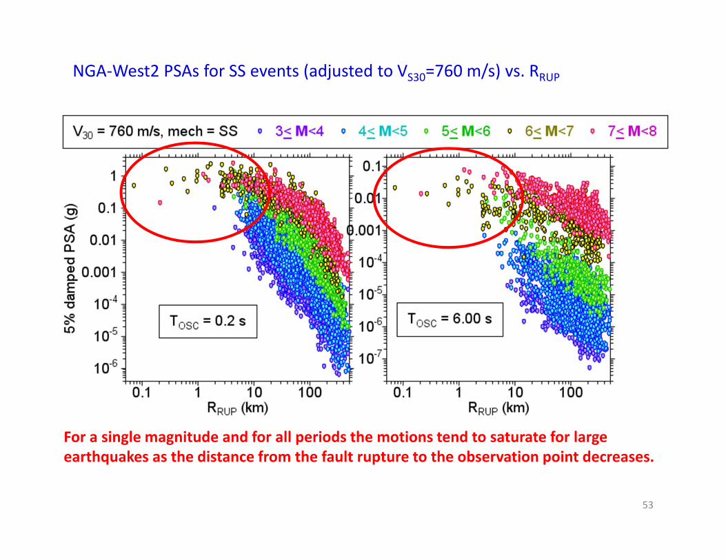
NGA‐West2 PSAs for SS events (adjusted to VS30=760 m/s) vs. RRUP
53
For a single magnitude and for all periods the motions tend to saturate for large earthquakes as the distance from the fault rupture to the observation point decreases.

NGA‐West2 PSAs for SS events (adjusted to VS30=760 m/s) vs. RRUP
54
At any fixed distance the ground motion increases with magnitude in a nonlinear fashion, with a tendency to saturate for large magnitudes, particularly for shorter period motions. To show this, the next slide is a plot of PSA within the RRUP bands vs. M.

NGA‐West2 PSAs for SS events (adjusted to VS30=760 m/s) vs. RRUP
55
At any fixed distance (centered on 50 km here, including PSA in the 40 km to 62.5 km range) the ground motion increases with magnitude in a nonlinear fashion, with a tendency to saturate for large magnitudes, particularly for shorter period motions. PSA for larger magnitudes is more sensitive to M for long‐period motions than for short‐period motions

NGA‐West2 PSAs for SS events (adjusted to VS30=760 m/s) vs. RRUP
56
For a given period and magnitude the median ground motions decay with distance; this decay shows curvature at greater distances, more pronounced for short than long periods.
(lines are drawn by eye and are intended to give a qualitative indication of the trends)

Characteristics of Data that GMPEs need to capture
• Change of amplitude with distance for fixed magnitude• Possible regional variations in the distance dependence• Change of amplitude with magnitude after removing distance dependence
• Site dependence (including basin depth dependence and nonlinear response)
• Earthquake type, hanging wall, depth to top of rupture, etc.
• Scatter
57

In 1994• Typical functional form of GMPEs
(Courtesy of Yousef Bozorgnia)
(Boore, Joyner, and Fumal, 1994)

Twenty years later…
(Courtesy of Yousef Bozorgnia)

• Need complicated equations to capture effects of:– M: 3 to 8.5 (strike‐slip)– Distance: 0 to 300km– Hanging wall and footwall sites– Soil VS30: 150‐1500 m/sec– Soil nonlinearity– Deep basins– Strike‐slip, Reverse, Normal faulting mechanisms– Period: 0‐10 seconds
• The BSSA14 GMPEs are probably the simplest, but there may be situations where they should be used with caution (e.g., over a dipping fault).
Courtesy of Yousef Bozorgnia)

Adding BSSA14 curves to data plots shown before

Example of comparison of horizontal GMPEs
Courtesy of Y. Bozorgnia

Example of comparison of horizontal GMPEs
3 3.5 4 4.5 5 5.5 6 6.5 7 7.5 8 8.5
M
0.0001
0.001
0.01
0.1
1
ASKBSSACBCYI
RJB=30, Strike-Slip, VS30=760
Courtesy of Y. Bozorgnia

Comparison of BSSA14 and BA08 AleatoryUncertainties
• ϕ= within‐earthquake • τ= earthquake‐to‐earthquake• σ= total ( )2 2

Vertical Component Results (Stewart et al., 2015) (SBSA15):
Compared to our horizontal‐component GMPEs• attenuation rates are broadly comparable (somewhat
slower geometric spreading, faster apparent• anelastic attenuation)• VS30‐scaling is reduced• nonlinear site response is much weaker• within‐earthquake variability is comparable• earthquake‐to‐earthquake variability is greater

V/H (SBSA15/BSSA14)
• V>H for short periods, close distances
• V/H generally less than 2/3 (“rule‐of‐thumb” value)
• V/H strongly dependent on Vs30 for longer periods (because of greater Vs30 scaling of H component)
• V/H not strongly dependent on M, in general

GMPEs: The Future
• Future PEER NGA Work • Using simulations to fill in gaps in existing recorded motions

NGA-West
Vertical-component GMPEs
Add directivity
NGA-East
GMMs for stable continental regions
2015
NGA-Sub
GMMs for subduction regions
2016
NGA: 2014 and beyond
Adapted from a slide from Y. Bozorgnia

New recordings may not fill data‐gaps in the near term, particularly close to large earthquakes and for important fault‐site geometries, such as over the hanging wall of a reverse‐slip fault.

New recordings may not fill data‐gaps in the near term, particularly close to large earthquakes and for important fault‐site geometries, such as over the hanging wall of a reverse‐slip fault.

New recordings may not fill data‐gaps in the near term, particularly close to large earthquakes and for important fault‐site geometries, such as over the hanging wall of a reverse‐slip fault.

Use of Simulated Motions
• Supplement observed data and derive GMPEs from the combined observed and simulated motions
• Constrain/adjust GMPEs for things such as:– Hanging wall– Saturation– Directivity– Splay faults and complex fault geometry– Nonlinear soil response

Using GMPEs in Building Codes
• For any site, find PSA at 0.2 s and 1 s that have a 2% in 50 year frequency of exceedance (this uses GMPEs)
• Map the resulting values (hazard maps)• Transform the hazard maps to design maps included in building codes

Design maps in building codes are for T=0.2 and T=1.0 s
• Design values at other periods are obtained by anchoring curves to the T=0.2 and T=1.0 s values, as shown in the next slide

0.0 0.5 1.0 1.5 2.0Period
0.0
0.5
1.0
1.5
2.0
2.5
Spec
tralR
espo
nse
Acce
lera
tion 0.0 0.5 1.0 1.5 2.0
0.0
0.5
1.0
1.5
2.0
2.5
Construct response spectrum at all periods using T = 0.2 and 1.0 sec values

Hazard Methodology Procedure Cartoon
a bEarthquake SourcesGround motion
d1
d2
d3
d4
r1
r2
r3
high seismicityzone
peak ground acceleration (pga)
Hazard curve
0.25g
a
M 7.6
distancepeak groun
d acceleratio
nM7.6
0.5g
The first step in making hazard maps: construct a hazard curve at each site

Source B
Source A Site
Annual probability that earthquake occurs:
Source A: 1/10 = 0.10Source B: 1/200 = 0.005
Constructing a hazard curve: a real example

Consider the uncertainty in motions from GMPEs

Consider the uncertainty in motions from GMPEs

Combine the source and ground‐motion uncertainties

Plot the resulting FOE for the PSA value

Do this for all possible ground motions from Source A to make a hazard curve for Source A

Combine hazard curves for all sources to make the final hazard curve

Pick off value for hazard map
2% probability of exceedance in 50 years

Make a map of the ground‐motion values for a given FOE; this is the hazard map that is the basis for the design maps included in building codes

Davis

FOE=0.0004 (~2500 year return period); T=0.2 s

FOE=0.0004 (~2500 year return period); T=0.2 s

FOE=0.0004 (~2500 year return period); T=1.0 s
Note: different M and R limits than on slide for T=0.2s

FOE=0.0004 (~2500 year return period); T=0.2 s

Note: different M and R limits than on slide for Davis at T=0.2s
FOE=0.0004 (~2500 year return period); T=0.2 s

FOE=0.0004 (~2500 year return period); T=1.0 s Note: different M and R limits than on slide for Davis at T=1.0 s

FOE=0.0004 (~2500 year return period); T=1.0 s

Some final remarks…

Thank You