Gross Worker Flows over the Business Cycle∗

Per Krusell† Toshihiko Mukoyama‡ Richard Rogerson§ Aysegul Sahin¶

June 2015

Abstract

We build a hybrid model of the aggregate labor market that features both stan-

dard labor supply forces and frictions in order to study the cyclical properties of gross

worker flows across the three labor market states: employment, unemployment, and non-

participation. Our goal is to assess the relative importance of frictions and labor supply

in accounting for fluctuations in labor market outcomes. Our parsimonious model is able

to capture the key features of the cyclical movements in gross worker flows and indicates

an important role for both frictions and labor supply.

∗This paper was previously entitled “Is labor supply important for business cycles?”. We thank Gadi Bar-

levy, Michael Elsby, and Marcelo Veracierto, in addition to seminar and conference participants at the Asian

Meeting of the Econometric Society (2011), Atlanta Fed, Chicago Fed, Minneapolis Fed, HEC Montreal, Hi-

totsubashi Macro Econometrics Conference, Federal Reserve Board, National University of Singapore, Search

and Matching Network Conference (2011), NBER Summer Institute (2011), NBER Conference on Macroe-

conomics Across Time and Space (2011), SED (2011), Oslo University, Norges Bank, European University

Institute, Bank of Korea, St. Louis Fed, San Francisco Fed, NBER Economic Fluctuations and Growth

Meeting (2011), University of Pennsylvania, University of Tokyo, and University of Washington for useful

comments. We thank Joe Song for excellent research assistance. Krusell thanks the NSF and the ERC

for financial support, Mukoyama thanks the Bankard Fund for Political Economy for financial support, and

Rogerson thanks the NSF and the Korean Science Foundation (WCU-R33-10005) for financial support. The

views expressed in this paper are solely the responsibility of the author’s and should not be interpreted as

reflecting views of the Board of Governors of the Federal Reserve System, Federal Reserve Bank of New York,

or of any other person associated with the Federal Reserve System. Corresponding author: Richard Rogerson,

Woodrow Wilson School, Princeton University, Princeton, NJ 08544; 609-258-4839, rdr@princeton.edu.†IIES, University of Goteborg, CEPR, and NBER‡University of Virginia§Princeton University and NBER¶Federal Reserve Bank of New York

1

1 Introduction

Modern research on aggregate labor market dynamics stresses the importance of micro-

founded models of labor market flows as a way to connect micro and macro data. In this

paper we build a parsimonious model of individual labor supply in the presence of labor

market frictions and assess its ability to account for gross worker flows between employment,

unemployment and non-participation over the business cycle.

Our model represents a hybrid of the two classes of benchmark models that dominate the

literature: heterogeneous agent models following in the spirit of Lucas and Rapping (1969),

and reflected in Chang and Kim (2006), and search models in the spirit of Mortensen and

Pissarides (1994). In the former, workers flow between employment and non-employment

and these flows represent optimal labor supply responses to changes in prices. In the latter,

workers are passive, always wanting to work but subject to frictions that sometimes prevent

them from working, thus generating flows between unemployment and employment. Reality

seems to reflect elements of both benchmarks, and to the extent that participation reflects

the desire to work, and unemployment reflects frictions that create a wedge between desired

and actual labor supply, we think the natural starting point for assessing a hybrid model of

labor supply is to confront it with data on the gross worker flows.

Our model features households subject to idiosyncratic shocks in the presence of incom-

plete credit and insurance markets and labor market frictions. Our specification of frictions

allows for endogenous search effort while non-employed, on the job search and heterogeneity

in match quality. We also include an unemployment insurance (UI) system that reflects key

features of the US system. Aggregating across heterogeneous households yields a model of

aggregate labor supply in the presence of frictions. We calibrate it so as to match steady

state levels of gross worker flows and assess the ability of specific aggregate shocks to generate

the cyclical patterns for gross worker flows that are found in the data.

We consider two types of exogenous aggregate shocks to labor market conditions: shocks

2

to labor market frictions, and shocks to wages, and calibrate them to have empirically rea-

sonable magnitudes. In the context of this model we ask three main questions. First, do the

outcomes—flows and stocks—move like they move the data? Second, how important are the

shocks to the different components of market conditions? And third, what role does labor

supply play?

We find that our benchmark model with shocks to frictions alone does a good job of

accounting for the key features of fluctuations in gross worker flows between the three labor

market states. We argue that the simulation results reflect some basic and intuitive economic

forces present in a model of labor supply in the presence of frictions. These mechanisms

actively involve the labor supply channel; even though the labor market participation rate

displays limited and only weakly procyclical movements, the gross flows in and out of not in

the labor force (N) into both employment (E) and unemployment (U) are large, volatile, and

show clear cyclical patterns. Although our benchmark model only has aggregate shocks to

frictions, the presence of on-the-job search implicitly incorporates an endogenous, procyclical

wage movement, as workers move up the job ladder more rapidly in good times. These

endogenous procyclical movements in wages give rise to important labor supply effects, so

the labor supply channel is important in allowing the model to match the behavior of gross

worker flows.

Heterogeneity is crucial to the model’s ability to account for the cyclical patterns in the

gross flow data. At any point in time, most workers are quite far from the boundary of

indifference between working and not working. However, a non-negligible group of workers

is close enough to indifferent that idiosyncratic or aggregate shocks can make them switch

participation status over the near term. This group turns out to be key for understanding

both gross flows and the movement of stocks over the cycle. It is thus important how our

model places restrictions on the size and composition of this group. Our calibration—the

selection of key parameters for utility, work payoff, and job availability—is designed to match

3

the average gross flows. The model’s implications for how these flows move in response to

aggregate shocks then rely to an important extent on its implications for how the sizes of

different groups move over the cycle.

Our paper is related to several strands in the literature. One of these is the literature

on gross flows.1 Another is the literature on individual labor supply in the presence of

frictions. Ham (1982) was an early effort to rigorously study unemployment in a labor

supply setting, showing that unemployment spells could not be interpreted as optimal labor

supply responses. Consistent with his findings, our model features both an operative labor

supply margin and unemployment, and unemployment is a departure from desired labor

supply. More recently, Low, Meghir, and Pistaferri (2010) study life cycle labor supply in

the presence of frictions. Our study is very much in the spirit of theirs, though because

our focus is on aggregate effects over the business cycle, our individuals are described in a

more stylized manner (without regard to age, etc.). Our own earlier work, e.g., Krusell et

al. (2010), is even more stylized and only looks at mechanisms in steady states, whereas the

present paper is focused entirely on aggregate fluctuations.2

A third strand is a recent literature that extends general equilibrium business cycle models

of employment and unemployment to allow for a participation decision.3 The key feature

that distinguishes our paper from these is our focus on gross worker flows—these papers only

consider labor market stocks. Alternatively, our model can be viewed as adding frictions

to the labor supply model of Chang and Kim (2006), which features idiosyncratic shocks,

indivisible labor, and incomplete markets.

1This includes, for example, Abowd and Zellner (1985), Poterba and Summers (1986), Blanchard and

Diamond (1990), Davis and Haltiwanger (1992), Fujita and Ramey (2009), Shimer (2012), and Elsby, Hobijn,

and Sahin (2015).2Our earlier work is significantly less detailed: it does not have UI, costly search, nor on the job search. Our

modeling of search costs here, moreover, actually allows us to fit the steady state flows significantly better.

Finally, note that due to the nonlinearity of our model, with wealth effects, cutoff decision rules, etc., it is not

sufficient to make steady state comparisons as a way of understanding how cyclical movements are generated.3These include Tripier (2004), Veracierto (2008), Christiano, Trabandt, and Walentin (2010), Galı, Smets,

and Wouters (2011), Ebell (2011), Haefke and Reiter (2011), and Shimer (2011).

4

An outline of the paper follows. In the next section we document the key business cycle

facts for gross worker flows among the three labor market states for the US over the period

1978–2009. Section 3 describes our theoretical framework and describes how we calibrate it.

Section 4 examines the cyclical performance of the model. Section 5 adds wage shocks to our

benchmark model and Section 6 concludes.

2 Worker Flows Over the Business Cycle

In this section we document the business cycle facts for gross worker flows. A model that

successfully accounts for the behavior of gross worker flows will necessarily account for be-

havior of the net flows and hence the three labor market stocks—E, U , and N , though not

vice versa. It follows that matching the behavior of the three labor market stocks is a less

stringent test of a model. Because it is much simpler to describe the behavior of the stocks

and they are subject to less measurement error, we think it is useful to examine the properties

of both the stocks and the flows in the models that we consider.

To begin our analysis, Table 1 presents summary statistics from the data for the business

cycle properties for the stocks.4 We use u to denote the unemployment rate, U/(E + U),

lfpr to denote the labor force participation rate, (E + U)/(E + U +N), and Y for GDP.

Table 1

Cyclical Properties of Stocks 1978-2009

u lfpr E

std(x) .1125 .0026 .0098

corrcoef(x, Y ) −.83 .36 .82

corrcoef(x, x−1) .93 .62 .91

The resulting patterns are relatively well known: employment is strongly procyclical, and

the unemployment rate is strongly countercyclical. Although the labor force participation

rate is procyclical, it is not as strongly cyclical as the other two series. The unemployment

4We restrict attention to the period 1978-2009 since that is the period for which we have consistent data

on gross flows. The cyclical components in Table 1 are isolated using an HP filter.

5

rate is the most volatile of the three series, and the labor force participation rate is the least

volatile. All three series are highly autocorrelated.

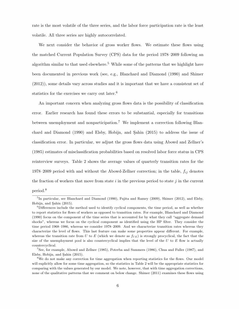
We next consider the behavior of gross worker flows. We estimate these flows using

the matched Current Population Survey (CPS) data for the period 1978–2009 following an

algorithm similar to that used elsewhere.5 While some of the patterns that we highlight have

been documented in previous work (see, e.g., Blanchard and Diamond (1990) and Shimer

(2012)), some details vary across studies and it is important that we have a consistent set of

statistics for the exercises we carry out later.6

An important concern when analyzing gross flows data is the possibility of classification

error. Earlier research has found these errors to be substantial, especially for transitions

between unemployment and nonparticipation.7 We implement a correction following Blan-

chard and Diamond (1990) and Elsby, Hobijn, and Sahin (2015) to address the issue of

classification error. In particular, we adjust the gross flows data using Abowd and Zellner’s

(1985) estimates of misclassification probabilities based on resolved labor force status in CPS

reinterview surveys. Table 2 shows the average values of quarterly transition rates for the

1978–2009 period with and without the Abowd-Zellner correction; in the table, fij denotes

the fraction of workers that move from state i in the previous period to state j in the current

period.8

5In particular, see Blanchard and Diamond (1990), Fujita and Ramey (2009), Shimer (2012), and Elsby,

Hobijn, and Sahin (2015).6Differences include the method used to identify cyclical components, the time period, as well as whether

to report statistics for flows of workers as opposed to transition rates. For example, Blanchard and Diamond

(1990) focus on the component of the time series that is accounted for by what they call “aggregate demand

shocks”, whereas we focus on the cyclical component as identified using the HP filter. They consider the

time period 1968–1986, whereas we consider 1978–2009. And we characterize transition rates whereas they

characterize the level of flows. This last feature can make some properties appear different. For example,

whereas the transition rate from U to E (which we denote as fUE) is strongly procyclical, the fact that the

size of the unemployment pool is also countercyclical implies that the level of the U to E flow is actually

countercyclical.7See, for example, Abowd and Zellner (1985), Poterba and Summers (1986), Chua and Fuller (1987), and

Elsby, Hobijn, and Sahin (2015).8We do not make any correction for time aggregation when reporting statistics for the flows. Our model

will explicitly allow for some time aggregation, so the statistics in Table 2 will be the appropriate statistics for

comparing with the values generated by our model. We note, however, that with time aggregation corrections,

none of the qualitative patterns that we comment on below change. Shimer (2011) examines these flows using

6

Table 2 reveals that the adjusted flows using Abowd and Zellner’s estimates of misclassi-

fication probabilities are systematically below their unadjusted counterparts. Put differently,

all three labor market states are more persistent than predicted by unadjusted flow rates.

As noted in the prior literature, flows that involve nonparticipation are affected much more

than other flows. Transition rates between employment and nonparticipation are approxi-

mately halved, while those between unemployment and nonparticipation are adjusted down

by around one third.

An alternative adjustment, suggested by Elsby, Hobijn, and Sahin (2015), involves re-

coding sequences of recorded labor market states to eliminate high-frequency reversals of

transitions between unemployment and nonparticipation. This procedure identifies individ-

uals whose measured labor market state cycles back and forth between unemployment and

nonparticipation from month to month and omits such transitions (“deNUN ification”). For

example, a respondent who reported a sequence of labor market states of NUN is recoded

as being a nonparticipant NNN . Elsby, Hobijn, and Sahin (2015) show that this correction

results in very similar transition rates between unemployment and nonparticipation to the

adjusted rates based on the Abowd and Zellner (1985) estimates. The average values of the

fUN and fNU transition rates with the adjusted data using deNUN ification were .146 and

.019, respectively. These values are very similar to the corresponding values in Table 2 (.137

and .021). In the remainder of our paper, we will use the average transition flow rates, as well

as labor market stocks, adjusted using the Abowd-Zellner estimates of misclassification as our

benchmark to assess the performance of our model while we will refer to both adjustments

when we evaluate cyclical performance of our model as we discuss below.

data that are corrected for time aggregation but finds the same cyclical properties as we do.

7

Table 2

Gross Worker Flows 1978–2009

Unadjusted Data Abowd-Zellner Correction DeNUN ified Data

FROM TO FROM TO FROM TO

E U N E U N E U N

E .957 .015 .028 E .972 .014 .014 E .957 .015 .028

U .261 .528 .211 U .235 .628 .137 U .263 .591 .146

N .048 .027 .925 N .023 .021 .956 N .048 .019 .933

Next we turn to the cyclical behavior of the gross flows. Table 3 presents summary statis-

tics from the data for the business cycle properties for gross flows data using the unadjusted

data as well as the Abowd-Zellner adjusted and deNUN ified flows data. The series are

quarterly, produced by taking the quarterly average of monthly series, and all series are then

logged and HP filtered.

Table 3

Cyclical Properties of Gross Worker Flows

Unadjusted Data

fEU fEN fUE fUN fNE fNU

std(x) .072 .034 .074 .051 .041 .061

corrcoef(x, Y ) −.68 .32 .78 .63 .60 −.68

corrcoef(x, x−1) .66 .23 .82 .69 .51 .76

Abowd-Zellner Correction

fEU fEN fUE fUN fNE fNU

std(x) .085 .083 .085 .104 .102 .071

corrcoef(x, Y ) −.62 .40 .74 .59 .52 −.20

corrcoef(x, x−1) .55 .29 .74 .60 .38 .29

DeNUN ified Data

fEU fEN fUE fUN fNE fNU

std(x) .069 .036 .076 .066 .042 .063

corrcoef(x, Y ) −.66 .29 .81 .55 .57 −.56

corrcoef(x, x−1) .70 .22 .85 .58 .48 .57

While there is a lot of information in this table, we focus our discussion around four basic

observations. First, although the stock of non-participants does not vary that much over

the business cycle relative to the other two stocks, Table 3 shows that the flows between

8

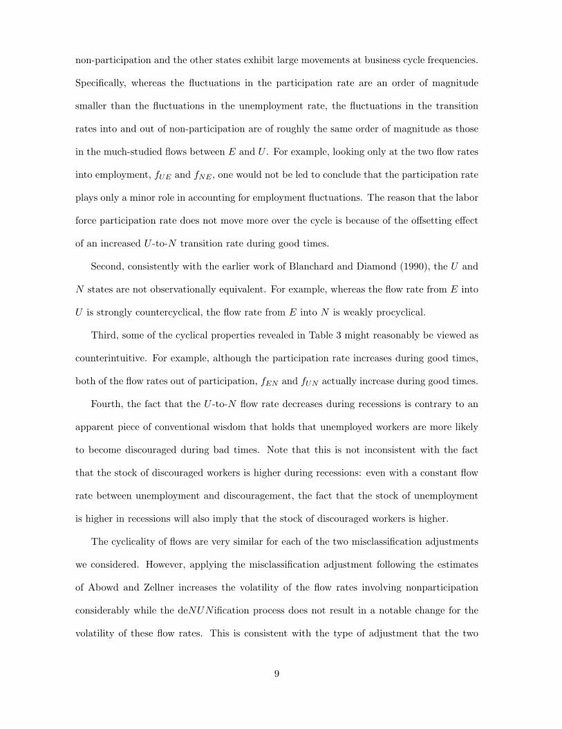
non-participation and the other states exhibit large movements at business cycle frequencies.

Specifically, whereas the fluctuations in the participation rate are an order of magnitude

smaller than the fluctuations in the unemployment rate, the fluctuations in the transition

rates into and out of non-participation are of roughly the same order of magnitude as those

in the much-studied flows between E and U . For example, looking only at the two flow rates

into employment, fUE and fNE , one would not be led to conclude that the participation rate

plays only a minor role in accounting for employment fluctuations. The reason that the labor

force participation rate does not move more over the cycle is because of the offsetting effect

of an increased U -to-N transition rate during good times.

Second, consistently with the earlier work of Blanchard and Diamond (1990), the U and

N states are not observationally equivalent. For example, whereas the flow rate from E into

U is strongly countercyclical, the flow rate from E into N is weakly procyclical.

Third, some of the cyclical properties revealed in Table 3 might reasonably be viewed as

counterintuitive. For example, although the participation rate increases during good times,

both of the flow rates out of participation, fEN and fUN actually increase during good times.

Fourth, the fact that the U -to-N flow rate decreases during recessions is contrary to an

apparent piece of conventional wisdom that holds that unemployed workers are more likely

to become discouraged during bad times. Note that this is not inconsistent with the fact

that the stock of discouraged workers is higher during recessions: even with a constant flow

rate between unemployment and discouragement, the fact that the stock of unemployment

is higher in recessions will also imply that the stock of discouraged workers is higher.

The cyclicality of flows are very similar for each of the two misclassification adjustments

we considered. However, applying the misclassification adjustment following the estimates

of Abowd and Zellner increases the volatility of the flow rates involving nonparticipation

considerably while the deNUN ification process does not result in a notable change for the

volatility of these flow rates. This is consistent with the type of adjustment that the two

9

correction procedures involve. The Abowd-Zellner correction is a time-invariant correction

method that applies the correction probabilities to any occurrence of the state N indepen-

dently while deNUN ification applies the correction to the high frequency reversals between

N and U . When we compare models to the data, we will report comparisons with the data

adjusted using both methods to provide a better assessment of the performance of our models.

For future reference we note a related finding in the recent work by Elsby, Hobijn, and

Sahin (2015). They go one step further than we do here by looking at, among other things,

the role of “worker attachment”. In particular, they find that the composition of the unem-

ployment pool shifts towards more attached workers during recessions; this factor accounts

for around 75 percent of the decline in the U -to-N transition rate during recessions. The most

important dimension of attachment turns out to be prior employment status. This feature

will be present in the quantitative model that we study. In fact, our relatively parsimonious

model will deliver natural explanations for all of the patterns just documented.

3 Labor Supply and Gross Worker Flows

The starting point for our analysis is a model of individual labor supply in the presence of

frictions that in steady state can match the key properties of the average gross worker flows.

Once we develop this model and calibrate it so as to match the average behavior of the gross

worker flows we will subject it to shocks to study its implications for fluctuations in the gross

worker flows.

Consider an individual with preferences given by:

Et

∞∑t=0

βt[log(ct)− αet − γst]

where ct ≥ 0 is consumption in period t, et ∈ {0, 1} is employment status in period t, and

st ∈ {0, 1} is a discrete variable that reflects whether the individual engages in active job

search in period t. The parameters α > 0, γ > 0 are the disutilities of work and active search

respectively and 0 < β < 1 is the discount factor. A key element of our model is that an

10

individual’s (net) return from work in the market is stochastic. In reality the relevant shocks

could influence both the reward to market work and the opportunity cost of market work,

but since it is ultimately the relative value of market work that matters, we capture this

with a single shock, which we model as an idiosyncratic shock to market productivity, zt.

We assume it follows an AR(1) process in logs:

log zt+1 = ρz log zt + εt+1

where the innovation εt is a mean zero, normally distributed random variable with standard

deviation σε.9

A salient feature of the data on gross worker flows that we presented in the previous

section is that even after cleaning the data to remove spurious flows, there remain large

movements of non-employed individuals between active and passive search. To capture this

in our model we assume that the disutility of active search, γ, is random. In our calibrated

model we assume that draws iid over time and distributed according to a uniform distribution

with mean γ and support {γ − εγ , γ, γ + εγ}.

The traditional literature on individual labor supply assumes that the relevant market

conditions faced by an individual are prices, most notably the wage rate (w) and the interest

rate (r). A key innovation of our labor supply model is to expand the set of market conditions

to also include four parameters—λu, λn, λe, and σ—that describe labor market frictions. We

will refer to λu, λn and λe as employment opportunity arrival rates: λu is the probability that

a non-employed individual who engages in active search receives an employment opportunity;

λn is the probability that a non-employed individual who does not engage in active search

receives an employment opportunity, and λe is the probability that an employed individual

receives an additional employment opportunity with another employer. The subscripts u

9Because z is mean-reverting, some movements in the return to market work will be predictable whereas

some will not. A richer model would include more detail, perhaps with part of the predictable component

reflecting age effects, and with multiple random components that differ in persistence. We view our approach

as a parsimonious first step.

11

and n reflect the fact that active search will determine whether an individual is counted as

unemployed or not in the labor force. The parameter σ is the employment separation rate

and is the probability that an individual employed in period t− 1 loses his or her job at the

beginning of period t. For now we assume that market conditions are constant over time;

when we consider business cycle fluctuations in a later section we will allow market conditions

to fluctuate.

An employed worker’s labor earnings is the product of three components: the market

wage per efficiency unit of labor services (w), the idiosyncratic worker component z described

above, and a match quality component (q). Whenever an individual receives an employment

opportunity, it is accompanied by a realization of the match quality q, which is an iid draw

from a log normal distribution with mean 0 and standard deviation σq. This value is fixed

for the duration of the match and is observed at the time the employment opportunity is

received.

There is a UI program, specified so as to capture key features of the UI system in the US

while also maintaining tractability. To be eligible for UI, a worker must have previously been

employed, and experienced an employment separation shock. That is, individuals who leave

employment by choice are not eligible. In order to receive benefits, we require that an eligible

individual engage in active search. Although we implicitly assume that the UI authority can

monitor search activity, we do not assume that the UI authority observes whether employment

opportunities are received or the associated match quality, so the receipt of benefits imposes

no restrictions on an individual’s decision to accept an employment opportunity. To capture

the fact that UI benefits have finite duration while minimizing the state space, we assume

that an eligible individual loses eligibility each period with probability µ. We will represent a

non-employed individual’s eligibility status by the indicator variable IB, with the convention

that a value of one indicates eligibility. Another feature of the UI system in the US is that

benefits are related to past earnings, subject to a cap. To capture this we assume that

12

an individual’s UI benefit is a linear function of his or her idiosyncratic shock z, up to a

maximum of b.10 Formally,

b(z) =

{b0z if b0z ≤ b

b otherwise.

We assume a market structure that is standard in the incomplete markets literature. The

individual cannot borrow and there are no markets for insuring idiosyncratic risk, but can

accumulate an asset, whose level we denote by a, and offers a rate of return given by r. To

capture the presence of various transfer programs that implicitly provide some insurance,

we assume that there is a proportional tax τ on labor earnings and a lump sum transfer T .

Combining these features, the individual’s period budget equation is given by:

ct + at+1 = (1 + r)at + (1− τ)wztqtet + (1− et)IBt st(1− τ)b(zt) + T

where, as above, et ∈ {0, 1} is the employment indicator.

Next we describe how events unfold within a period. At the beginning of period t an

individual will observe new realizations for z, γ, and IB. To detail the subsequent events

we need to distinguish individuals according to three scenarios. In the first scenario, the

individual was not employed in the previous period and did not receive an employment

opportunity while searching. In the second scenario, the individual was not employed in the

previous period but did receive an employment opportunity and associated match quality

while searching. In the third scenario, the individual was employed in the previous period.

We begin with the individual in the first scenario. Having received new realizations for z,

γ, and IB, this individual chooses whether to engage in active or passive search and makes

a consumption saving decision. Following these decisions, the outcome of search will be

realized. If the individual receives an employment opportunity (and an associated draw of

match quality) he or she will enter period t+ 1 as an individual in scenario two.

10We index benefits to z rather than past earnings in order to economize on the state space while still

allowing for feedback from market opportunities to UI benefits.

13

Next consider an individual who enters the current period in scenario two. This indi-

vidual begins the period with an employment opportunity in hand. If the individual ac-

cepts the employment opportunity they will work this period, receive labor earnings, make

a consumption-savings decision and enter the subsequent period as an individual in scenario

3. If the individual chooses to reject the employment opportunity, they are now identical to

an individual who entered the period under scenario one, and once again makes choice about

search effort, consumption and saving.

Finally, we consider an individual who enters the period in scenario three. In the process

of transiting from the previous period to the beginning of this period we allow for two types

of developments. First, we implicitly assume that employed workers engage in passive search

and hence may receive additional employment opportunities. Second, as noted earlier, we

allow for the possibility that past employment positions are destroyed, causing the worker

to be separated. While there are various ways that one could formulate the joint outcomes,

we assume that this individual experiences one of four mutually exclusive events as follows.

With probability 1−σ−λe the individual retains their previous employment opportunity and

does not receive an additional opportunity. With probability λe the individual retains their

previous opportunity but also receives an additional employment opportunity with an iid

draw from the match quality distribution. With probability σλu the individual is separated

from their previous employment opportunity but receives a new employment opportunity

with a new draw from the match quality distribution.11 Lastly, with probability σ(1−λu) the

individual is separated from their previous employment position and does not simultaneously

receive a new employment opportunity.

11We interpret these individuals as the very short-term unemployed, who find a job within the month of

separation, which is the main reason we use λu for the probability of new offer. Alternatively, we could have

set this probability equal to σλe, on the grounds that a separating worker has the same chance of getting

an outside offer within the period as does a non-separating worker. As a practical matter this makes little

difference, but our choice captures the possibility that a separating worker may be able to generate additional

offers through contacts. More generally we could have introduced another independent parameter to capture

this probability.

14

In the event that the individual has only one employment opportunity, the situation is

identical to scenario two. In the event that the individual has two employment opportunities,

it is optimal to take the one with the higher match quality and discard the other, at which

point they are again like an individual in scenario two. Note that the combination of on-

the-job search and heterogeneous match quality implies that our model features a job ladder

in which employed individuals tend to transition to higher paying jobs over time. Finally, if

the individual is separated and has no employment opportunity, they are then identical to

an individual in scenario one.

We formulate the individual’s decision problem recursively. We formulate the problem at

the point where all new shocks have been realized, so that the individual knows their current

value of z, their current value of γ, whether they have an employment opportunity and if so

the value of the match quality, their current UI eligibility status, and the assets brought into

the period.

An individual without an employment opportunity (i.e., what we called scenario one

above) decides both whether to engage in active or passive search and on consumption versus

saving. Let U(a, z, γ, IB) and N(a, z, γ, IB) denote the Bellman values for such an individual

conditional upon active search (i.e., unemployed) and passive search (i.e., out of the labor

force), respectively. An individual in this “jobless” situation will have a value denoted by

J(a, z, γ, IB) that is simply the maximum of these two options:

J(a, z, γ, IB) = max{U(a, z, γ, IB), N(a, z, γ, IB)}

An individual with an employment opportunity (i.e., what we called scenario two above)

has an additional decision: whether to accept or reject the employment opportunity. An

individual who rejects the employment opportunity will become identical to an individual

who did not have an employment opportunity, and hence receive the value J(a, z, γ, IB).

Let W (a, z, q, IB) denote the Bellman value for an individual who accepts an employment

15

opportunity. An individual with an employment opportunity will choose the maximum of

these two values, which we will denote by V (a, z, q, γ, IB):

V (a, z, q, γ, IB) = max{W (a, z, q, IB), J(a, z, γ, IB)}.

Having developed the notation for all of these Bellman values we can now write out the

individual Bellman equations that define these values. Working backwards from the end of

the period decisions, the Bellman equation for W is given by:

W (a, z, q, IB)

= maxc≥0,a′≥0

{ln c− α+ βEz′,q′,γ′ [(1− σ − λe)V (a′, z′, q, γ′, 0) + λe{V (a′, z′,max{q, q′}, γ′, 0)

+σ{(1− λu)J(a′, z′, γ′, 1) + λuV (a′, z′, q′, γ′, 1)}]}

subject to

c+ a′ = (1 + r)a+ (1− τ)wzq + T.

The future terms on the right-hand side reflect the four mutually exclusive events discussed

previously that can transpire between the end of this period and the beginning of the following

period for an individual who works today.

Next consider the Bellman equations for active and passive search. For active search we

have:

U(a, z, γ, IB) = maxc≥0,a′≥0

{ln c−γ+βEz′,q′,γ′,IB′ [λuV (a′, z′, x′, γ′, IB′)+(1−λu)J(a′, z′, γ′, IB′)]}

subject to

c+ a′ = (1 + r)a+ (1− τ)IBb(z) + T,

and for passive search:

N(a, z, γ, IB) = maxc≥0,a′≥0

{ln c+ βEz′,q′,IB′ [λnV (a′, z′, q′, γ′, IB′) + (1− λn)J(a′, z′, γ′, IB

′)]}

16

subject to

c+ a′ = (1 + r)a+ T.

Our model provides a clear mapping to the data with regard to classifying a worker as

either employed, unemployed, or out of the labor force. Specifically, an individual who works

in period t is labeled as employed. An individual who is not employed in period t, but

engages in active search during period t is labeled as unemployed. The residual category, an

individual who is not employed in period t and does not engage in active search, is labeled

as out of the labor force.

To generate implications for aggregate gross worker flows we assume that there are a

large number of workers, each of whom is just like the individual described above, with all

of the shock realizations being iid across individuals. Given a set of market conditions (i.e.,

prices and frictions), we can then look for a stationary distribution of individuals. In this

stationary distribution there is an invariant distribution of individuals over the individual

statevariables, an invariant distribution of individuals over the three labor market states

o(employment, unemployment and out of the labor force), and an invariant distribution over

gross flows.

3.1 Calibrating the Stationary Distribution

This section describes our procedure for calibrating the parameters of our model so that the

stationary distribution with constant market conditions matches the gross worker flows in

the data. The numerical solution methods are explained in Appendix A.2.

The model has a large number of parameters that need to be assigned: preference pa-

rameters β, α, γ and εγ , idiosyncratic productivity shock parameters ρz and σε, the variance

of the match quality shock σq, frictional parameters (σ, λu, λe, and λn), the tax rate τ , the

transfer T , the parameters of the UI system (b, b, and µ), and prices (r and w). Because

data on labor market transitions are available monthly, we set the length of a period to be

17

one month.

Several parameters are set without solving the model. As is standard in the literature,

we set β to be consistent with a discount factor of .96 at an annual level, implying β =

.9947. We calibrate the shock process z to estimates of idiosyncratic wage shocks, and so

assume an AR(1) process, with ρ = .997 and σ = .098. Aggregated to an annual level

this would correspond to persistence of .96 and a standard deviation of .206, which we take

as representative values from this literature.12 Note that the tax rate on labor income is

inconsequential, since it effectively amounts to a renormalization of the wage. We introduce

it as a way to generate the revenue for the lump-sum transfer and UI system in an internally

consistent manner. In line with various studies, we set τ = .30.13 The lump sum transfer T

will be set so that the government budget balances in steady state equilibrium.

The parameters of the UI benefit system are chosen as follows. First, the parameter µ

is set to 1/6 so that the average duration of benefits is equal to six months. We set the

cap on benefits to be 46.5 percent of the average wage in our steady state equilibrium. In

our model, all exogenously separated individuals are eligible for UI, and will collect if they

are unemployed and search actively. In reality, many exogenously separated individuals may

either not be eligible or choose not to apply. To incorporate this we set our replacement rate

b so that total UI payments in steady state is in line with the data. Over the 1978–2009

period, total UI payments are .69 percent of total compensation and .85 percent of total

wages and salaries. We use a replacement rate of .23, which results in the total UI payments

of .74 percent of total earnings.

The remaining parameters are chosen so that the steady state equilibrium matches specific

12See for example, estimates in Card (1994), Floden and Linde (2001), and French (2005). Given that the

wage process consists of z and q in the model (and there is also an endogenous selection of employed workers),

the wage process does not exactly correspond to the z process. However, it turns out that the discrepancy

is small (the estimated value of the persistence parameter from the model-generated data is .984 and the

standard deviation is .109).13Following the work of Mendoza, Razin, and Tesar (1994) there are several papers which produce estimates

of the average effective tax rate on labor income across countries. Minor variations in methods across these

studies produce small differences in the estimates, but .30 is representative of these estimates.

18

targets. Although this amounts to a large set of nonlinear equations which is solved jointly,

we think it is informative to describe the calibration as a few distinct steps.

We begin with the five parameters α, γ, σ, λu, and λn. We discipline the value of γ

relative to the value of α based on measures of search time relative to working time. In

particular, since average time devoted to search for unemployed workers is approximately

3.5 hours per week, and average hours of work for employed individuals are approximately

40, we set γ = 3.540 α. Intuitively, holding all else constant, the disutility from working α will

directly affect the desire of individuals to work and hence exerts a direct influence on the

employment rate. The gap between λe and λn will influence how the non-employed are split

between active and passive search. For a given gap, the level of λn will directly impact on

the flow from N to E. And the value of σ will intuitively have a direct impact on the flow

from E into U . Accordingly, we set the values of α, σ, λu, and λn so as to match the labor

force participation rate (.67), the unemployment rate (.065), the EU flow rate (.014) and the

NE flow rate (.023). All these values are averages from 1978 to 2009.

The two parameters λe and σq will directly impact the nature of job-to-job transitions in

the model. Accordingly, we set these two values so as to match a job-to-job transition rate

of 1.4% per month and an average wage gain upon experiencing a job-to-job transition of

3.3%. These targets are drawn from Tjaden and Wellschmied (2014).

The final preference parameter to be determined is εγ , which governs the variation in the

disutility associated with active search. This parameter plays a very specific role in terms of

allowing our model to match the patterns in gross worker flows. As noted previously, a key

feature of the gross flow data is that even after correcting for potential spurious flows due

to misclassification, there are still large flows between U and N . Taking these flows at face

value, they suggest important temporary shocks that influence the decisions of non-employed

individuals. We generate these flows by assuming a shock to the disutility of active search.

While this could reflect real demands on an individual’s time that make search more costly,

19

it could also reflect psychological effects associated with the job search process. We set εγ so

as to match this aspect of the gross flow data.

The above steps are carried out for given values of r and w. As is well known in this type

of model, the gap between r and β is an important determinant of capital accumulation.

And given a value for r the value of w will influence the relative payments to labor and

capital. While our subsequent analysis is partial equilibrium, we impose that our steady

state values for r and w are consistent with factor prices generated from a Cobb-Douglas

aggregate production function with capital share parameter equal to .30 assuming factor

inputs are those implied by our steady state model. This procedure implies r = .0033 and

w = 2.74. The government budget balance condition then implies that T = 1.53.

Table 4 summarizes values for the other calibrated parameter values and Table 5 displays

the implications for steady state gross flows in our calibrated model, as well as the corre-

sponding average values for these flows for the US over the period 1979–2009. We report the

95% confidence intervals for the flow rates in the data that were calculated using bootstrap-

ping on the microdata. Further details regarding data sources and the construction of labor

market flows are provided in Appendix A.1.

Table 4

Calibration

Parameter Values

β ρz σε µ α γ λu λn σ λe σq εγ.9947 .997 .098 1/6 .425 .037 .275 .204 .0178 .054 .036 .026

20

Table 5

Gross Worker Flows in the Data and the Model

Abowd-Zellner Adjusted Data Model

FROM TO FROM TO

E U N E U N

E .972 .014 .014 E .973 .014 .013

95% CI (.970, .973) (.013, .015) (.013, .016)

U .235 .628 .137 U .215 .663 .122

95% CI (.218, .254) (.607, .649) (.120, .154)

N .023 .021 .956 N .023 .017 .959

95% CI (.020, .025) (.018, .023) (.954, .960)

While the nonlinear nature of the model prevents a perfect match to the gross flow data

given the number of free parameters and the additional moments being matched, Table 5

indicates that the model does a very good job of matching the gross flows found in the

data. Almost all flow rates lie within the 95% confidence interval for the flow rates. To the

best of our knowledge, ours is the first structural model to present such a close fit to these

data. Previous work has not been able to provide such a close match to the flows between

unemployment and nonparticipation, and since flows must sum to one, these earlier studies

have necessarily missed on the other flows as well.

4 Fluctuations in Gross Worker Flows

Our main goal is to examine the extent to which our labor supply model of gross worker flows

can match the properties of fluctuations in Tables 1 and 2 when subjected to empirically

reasonable shocks to market conditions. Our initial exercise will assume that the only source

of shocks is to frictions, i.e., we will assume that the two prices—w and r—remain constant.

This exercise is of particular interest, since many researchers, e.g., Hall (2005), have argued

that a model in which wages are perfectly rigid offers a good account of labor demand

movements in the sense that it accounts for cyclical movements in the job finding rate in

a model with a fixed labor force. In this section we will take as given the fluctuations in

frictions found in the data and ask whether such a model also provides a good account of

21

labor market flows in a model that explicitly allows for an endogenous participation margin.

4.1 Modeling Shocks to Market Conditions

There are a few different ways that we could proceed. One strategy would be to estimate

the model using some type of simulated moments estimator on time series data. We instead

adopt a much simpler and, we think, more transparent approach that offers some important

insights into the role that different driving forces play in shaping the cyclical properties of

gross worker flows. Specifically, given that our focus is on business cycle fluctuations and

that a key feature of business cycles is comovement among series, we effectively focus on

perfectly correlated movements in market conditions that reflect business cycle movements.

We then ask whether such movements can account for business cycle fluctuations in gross

worker flows if the relative variances of the movements in each variable are set to empirically

reasonable values. Intuitively, we want to consider shocks to labor demand that manifest

themselves in fluctuations in prices and frictions.

The simplest implementation of this method would posit a latent aggregate state s that

follows a Markov process, with prices and frictions all being functions of this latent aggregate

state s.14 As is common in the business cycle literature with heterogeneous agents, we assume

that the shocks to market conditions follow a two state Markov process. We will refer to one

state as the “good” state (denoted by a superscript G) and the other state as the “bad” state

(denoted with a superscript B). The good state will have a high value for the employment

arrival rates λu, λe and λn, and a low value for the employment separation rate σ. We

denote the two possible realizations for the market conditions shock as (λGu , λ

Gn , λ

Ge , σ

G) and

(λBu , λ

Bn , λ

Be , σ

B). We parameterize these shocks as λGu = λ∗

u+ελ, λBu = λ∗

u−ελ, σG = σ∗−εσ,

and σB = σ∗ + εσ, where λ∗u and σ∗ are the values for the model calibrated to match

average transition rates. We assume that movements in λe and λn are such as to maintain

14More generally, one might consider a specification in which the innovations are perfectly correlated but

in which the individual components display different degrees of persistence.

22

constant ratios relative to λu. We assume that the transition matrix for the Markov process

is symmetric, with diagonal element denoted by ρ.

In our model, both the level and fluctuations in fUE closely mimic the level and fluctu-

ations in λu. For this reason we choose the value of ελ so that the fluctuations in fUE in

the simulated model match the standard deviation of the fluctuations in fUE found in US

data. This leads to ελ = .0632. Given values for the λi’s, which influences the impact of

time aggregation on measured fEU , the level and fluctuations in fEU closely follow the level

and fluctuations in σ, so we choose εσ = .0025 so as to match the fluctuations in fEU . We

match the volatility values based on the Abowd-Zellner correction procedure. The value of

ρ is set to .983.

4.2 Cyclical Properties of Stocks

We begin with the less stringent test in which we assess the ability of the model to match the

cyclical movements in the three labor market stock variables—employment, the unemploy-

ment rate, and the participation rate. Table 6 shows the results for the benchmark model and

the data. To compute correlations with output in our partial equilibrium model we generate

a series for output by taking our model generated series for capital and efficiency units of

labor and using them as inputs into a Cobb-Douglas production function with capital share

parameter of .30.

Table 6

Behavior of Stocks in the Data and the Model

Data Model

u lfpr E u lfpr E

std(x) .1125 .0026 .0098 .118 .0020 .0089

corrcoef(x, Y ) −.83 .36 .82 −.99 .15 .99

corrcoef(x, x−1) .93 .62 .91 .88 .66 .89

Table 6 reveals that our model of labor supply with shocks to frictions as the sole driving

force does a very good job of accounting for the behavior of the three labor market stocks,

23

not only qualitatively but also quantitatively. The key result here is that the behavior of

the participation rate in the model closely matches its behavior in the data. In a two-

state model with an exogenously fixed participation rate, shocks to job-finding and job-

loss rates that match the movements in the data will necessarily provide a close match to

observed movements in E and U precisely because movements in participation are modest in

comparison to movements in employment. The key issue then is whether our model featuring

an endogenous participation margin will generate empirically reasonable movements in the

participation rate. Table 6 shows that our model is able to account for roughly 80 percent

of movements in the participation rate, as well as the modest procyclical nature of these

fluctuations.

It is important to emphasize that it is not clear a priori that this model would match

even the qualitative features of participation rate fluctuations. The reason for this is that

there are several competing forces. In a much simpler model, Krusell et al. (2010) show that

holding all else constant, decreases in job-finding rates and increases in job-separation rates

lead to less time spent in employment, thereby lowering income. This decrease in income

leads to a negative wealth effect on labor supply, as individuals seek to increase time spent

working in order to compensate for the loss in income. Individuals who desire to work more

will be more likely to engage in active search when not employed, and will be less likely to

leave a job when employed. These responses tend to generate a countercyclical participation

rate.

But another force works in the opposing direction. In this model, participation for a

non-employed worker represents an investment decision, in that a worker needs to pay the

up-front cost associated with active search in order to generate a potential flow of income

associated with successful job search. In good times there are three factors tending to increase

the return on this investment. First, the probability of a successful search is greater. Second,

the fact that separation rates are lower implies that a job match will last longer. Third,

24

because arrival rates of outside opportunities for employed workers are higher, the prospects

for wage increases via job-to-job transitions are greater. These three factors make it more

likely that the individual will engage in active search in good times, leading one to expect

procyclical participation.

There are also effects that interact with the presence of UI benefits. In bad times there

is an increase in separations, and these workers are all assumed to be eligible for UI. But

collecting UI requires active search. Benefits may induce some individuals to search actively

who otherwise would not. On the other hand, lower arrival rates of jobs in bad times can

increase the probability that benefits expire for an individual, which may lead to fewer

individuals receiving benefits.

Despite the opposing forces at play, Table 6 shows that our model not only matches the

key qualitative properties found in the data, but also does a good job quantitatively. While

the model does somewhat underpredict the size of fluctuations in the participation rate, a

point we shall return to later, we view the results in Table 6 as a significant success for the

model.

4.3 Cyclical Properties of Gross Flows

We next consider the more stringent test of whether the model is able to account for the key

patterns in the gross flows that underlie these patterns for the stocks. Table 7 displays the

key business cycle facts about the gross flows in the data and in the model. While we targeted

the volatility of fEU and fUE using the Abowd-Zellner adjusted data, we also include the

data based on the alternative adjustment.

25

Table 7

Gross Worker Flows in the Data and the Model

A. Abowd-Zellner Adjusted Data

fEU fEN fUE fUN fNE fNU

std(x) .085 .083 .085 .104 .102 .071

corrcoef(x, Y ) −.62 .40 .74 .59 .52 −.20

corrcoef(x, x−1) .55 .29 .74 .60 .38 .29

B. DeNUN ified Data

fEU fEN fUE fUN fNE fNU

std(x) .069 .036 .076 .066 .042 .063

corrcoef(x, Y ) −.66 .29 .81 .55 .57 −.56

corrcoef(x, x−1) .70 .22 .85 .58 .48 .57

C. Model

fEU fEN fUE fUN fNE fNU

std(x) .085 .069 .085 .036 .047 .060

corr(x, Y ) −.79 .08 .69 .91 .52 −.97

corr(x, x−1) .77 .13 .71 .67 .67 .90

The model is able to account for the key cyclical patterns: it captures the counter-

cyclicality of unemployment inflows (E-to-U and N -to-U flow rates), the procyclicality of

unemployment outflows (UE and UN flow rates) and the procyclicality of flows between

E and N . Although the model is very successful in replicating the cyclicality of the flows,

there are some discrepancies between the data and the model in terms of the magnitudes

of fluctuations for some of the flows. However, it is important to note that the alternative

method for correcting for classification error (what we refer to as “deNUN ification”) implied

levels of volatility that are much more in line with those predicted by our model. In view

of this we feel that the discrepancies in volatility levels in Table 7 should not be viewed as

particularly problematic. In what follows we focus on the describing the economics behind

the cyclicality patterns.

Some of these cyclical patterns in the gross flows are quite intuitive and so do not merit

much discussion. For example, the procyclical flow rate from U to E is mechanically driven

by the procyclical shocks to λu, and the countercyclical flow from E to U is mechanically

driven by the countercyclical pattern in the shocks to σ. However, as noted earlier, we

believe that two of the patterns that the model is able to replicate are at least somewhat

26

counterintuitive. Specifically, during good times the flows from E to N and U to N are both

higher, despite the fact that the stock of workers in N is countercyclical. In what follows we

describe the economics behind these patterns.

In thinking about the response of flows to a change in market conditions it is useful to

distinguish two broad types of effects. At any point in time, individuals are distributed across

the space of individual state variables. For a given set of market conditions, decision rules

partition this space into the three labor market states E, U , and N and gross flows result

from individuals crossing the boundaries between these regions. Hence a key determinant

of these flows will be the mass of individuals who are near the boundary. When market

conditions change, the boundaries of these regions change, and some individuals will change

states even conditional on not experiencing any change in their individual state variables.

Note, however, that these are essentially one time changes in flows, in the sense that once

the boundaries have adjusted and individuals are reclassified, going forward in time the flows

will again be dictated by the mass of individuals crossing fixed boundaries. While both one-

time and persistent effects will shape the resulting correlation patterns, in the presence of

persistent shocks to market conditions the correlations will intuitively be dominated by the

persistent responses, which reflect movements of individuals across boundaries, rather than

the movements in the boundaries themselves.

We start with the flow from U to N . To understand this change it is essential to consider

the changing composition of the unemployed. In particular, the key dynamic is that the

composition of this group shifts toward individuals who are less attached to work (i.e., close

to the boundary of indifference between U and N), thereby increasing the the fraction of

unemployed individuals who cross the boundary into nonparticipation.15 To see why, note

that in good times unemployed workers exit to employment more quickly, so the pool of

15In fact, for a given distribution of workers in the unemployment pool the immediate impact of a decrease

in frictions is to expand the participation region (i.e., shrink the region of state space that maps into N)

and decrease the fraction who cross from U into N . But the resulting dynamic effects associated with lower

frictions changes the composition of the unemployment pool and increases the U to N flow.

27

unemployed individuals is relatively more composed of individuals who have just entered

unemployment. Since employed workers are less likely to enter unemployment in good times

(recall that the job separation probability decreases in good times), new entrants to unem-

ployment are dominated by individuals that transition from N to U . But these individuals

are more likely to be close to the boundary, making them more susceptible to a transition

that puts them back in the N state. This model feature is consistent with Elsby, Hobijn, and

Sahin (2015), who show that the composition of the unemployed pool shifts towards more

“attached” workers during recessions, where the most important dimension of attachment is

prior employment status. They show that this mechanism accounts for around 75 percent of

the decline in the UN flow rate during recessions.

Next we consider the flow from E to N . In the model this flow is very weakly procyclical.

Note also that similar to the data, this flow exhibits very little serial correlation. These two

properties stem from the fact that the persistent response in the EN flow turns out to be very

close to zero, so that the statistics for this flow are dominated by the immediate one-time

changes in flows that are associated with the change in boundaries defined by the decision

rules.16 To understand these effects it is important to note that there is an option value

associated with staying employed. In particular, an employed individual understands that

after a quit and hence a transition to N , it will be costly to return to E in the future (due to

search costs and/or the time it takes to receive an employment opportunity). It follows that

an employed individual needs to consider this option value when deciding whether to remain

employed. As is standard in such a setting, an individual will remain employed even when

it is “statically” suboptimal, on account of the option value of staying employed. When an

aggregate shock decreases the level of frictions, the implicit costs of finding employment go

down, and the option value diminishes. This results in a one time flow from E into N .

16The small persistent effect in turn reflects the combined effect of several small effects, including compo-

sitional effects and changes in wealth.

28

Lastly we consider the NU and NE flows. In the model the former flow is countercyclical

and the latter is procyclical, as in the data. To see why the model delivers this pattern, note

that the primary source of flows from N into U or E is those individuals who are close to the

boundary but on the N side. A small shock to individual state variables could push such an

individual across the boundary and into the U or E regions. For an individual to flow into

U , the individual must not receive an acceptable employment opportunity in the meantime,

since this will take them from N into E instead. But during good times the increase in job

opportunity arrival rates implies that marginal N workers are more likely to receive offers

that take them into E, thus decreasing the flow of these workers into U .

The above analysis assumed that there were aggregate shocks to both the job finding

rates and to the job loss rates. It is also of some interest to assess the relative importance

of these two types of shocks. To evaluate this we use the identical parameterization of the

model but then simulate the model with the business cycle shock to the job-loss rate shut

down. In the interest of space we do not present the detailed results, but instead offer a

brief summary. For the behavior of the three labor market stocks the main finding is that

this specification reduces the volatility of both the unemployment and employment rates by

about one third relative to the benchmark, with a much smaller decrease (roughly 10%) in

the volatility of the participation rate.

The behavior of the gross flows are relatively unaffected with two exceptions. The first

is the volatility of fEU . Not surprisingly, with shocks to σ shut down the volatility of fEU

is reduced dramatically. However, the time aggregation implicit in our model specification

does lead to countercyclical movements in fEU even in the absence of shocks to σ, though

this effect accounts for only about 20 percent of the movement in fEU . The other notable

difference is that the volatility of fUN is reduced in half relative to the benchmark model.

This is consistent with the explanations that we have articulated above. Specifically, we

argued that the procyclical movement in fUN resulted from a composition bias, due to the

29

fact that in good times the unemployment pool was increasingly composed of individuals

who entered U from N . But the decrease in the job-separation rate during good times was

one of the factors that influenced the size of this composition effect, since in good times it

served to reduce the number of individuals in U who entered from E. It follows that shocks

to the job loss rate are important in shaping the observed behavior of flows between U and

N .

4.4 Summary

The above discussion has focused on describing the intuition for the qualitative patterns

found in Table 7. We conclude that the economics implicit in the model that is responsible

for these patterns is quite straightforward, and for this reason we think the results are a

robust feature of our relatively parsimonious labor supply model of worker flows. Of course,

the extent to which the model can reproduce the quantitative features of fluctuations in gross

flows depends not only on the qualitative patterns but also the quantitative magnitudes of

the various effects. It is reasonable to think that a key factor for the quantitative results is the

mass of individuals that are near the participation boundary. In this regard, the discipline

in our quantitative work derives from the fact that our steady state model is consistent with

the average level of gross flows.

5 Wage Shocks

The preceding analysis indicates that shocks to labor market frictions alone in our model of

labor supply give rise to economic mechanisms that qualitatively and quantitatively capture

many of the salient patterns in the movements of gross worker flows over the business cycle.

Nonetheless, since the model was only able to generate about 80 percent of the fluctuations in

the participation rate, in this section we examine the effects of adding an additional shock to

market conditions, namely a shock to the wage rate per efficiency unit of labor. Intuitively,

standard intertemporal labor supply responses suggest that procyclical wages will lead to a

30

procyclical response in the desire to work, suggesting a procyclical response in participation

in our model, a response that will primarily occur through the impact on the indifference

boundaries of workers. In this section we examine these responses quantitatively.

As a first step it is relevant to consider movements in real wages in the data and in our

benchmark model. As is well known, many measurement issues come into play when measur-

ing the cyclicality of average real wages in the data. There are two commonly used measures

of wages in macro studies. The first measure is the average hourly earnings of production

and nonsupervisory employees in the private sector and is based on the establishment survey.

The second measure is real compensation per hour in the nonfarm business sector, based on

the productivity and costs releases.17 We calculate the volatility of wages for the 1978–2009

period using each of these two measures. When we use the first measure we deflate the

average hourly earnings using both the consumer price index (CPI) and the GDP deflator,

which also matters. We find that the standard deviation of average hourly wages is .0083

when deflated with the CPI and .0049 when deflated with the GDP deflator. When we use

the real compensation measure, the two analogous figures are .0111 and .0102. However, a

key issue for our purposes is the extent to which these movements in real wages are correlated

with the cycle. In fact, these wage movements display very little correlation with GDP when

one compares the cyclical components from an HP filter: for the four different real wage

series noted above, the correlations with GDP range from −.089 to −.005. If we regress the

cyclical component of real wages on GDP and several lags, the standard deviation of the

predicted part of the real wage series is .003. We will use this as our benchmark target in

the experiment that follows.

We previously noted that the presence of a job ladder in our model combined with pro-

cyclical job-finding rates implicitly leads to procyclical average wages even if the wage per

efficiency unit is constant over time. In our benchmark specification in the previous section

17For example, Gertler and Trigari (2009) use the first measure while Galı (2011) use the second one. Galı

(2011) shows that these two measures have different implications for wage inflation.

31

the standard deviation of the of the average wage is roughly .002, and has a correlation of

.52 with output. Roughly half of this procyclicality of the wage is due to the procyclicality

of average match quality, with the other half due to the fact that fewer high productivity

workers lose their jobs during good times. Even with a very conservative interpretation of

the data on average wage movements over the business cycle, this suggests that there is scope

for additional movements in wages. In what follows we will consider wage shocks that are

0.5% higher in the good state and 0.5% lower in the bad state. In the results reported below,

the standard deviation of the average wage increases by roughly 50 percent, to .0029, with

a correlation of .75 with GDP. Interestingly, because the procyclical movement in the wage

per efficiency unit will induce additional individuals to participate, we find that the average

value of z turns from mildly procyclical to mildly countercyclical.18

The model remains exactly as before and the calibration of the steady state is identical.

The only change is that when we consider business cycles we assume that the wage per

efficiency unit of labor moves together with the labor market frictions, and so takes on two

values: wG and wB. Given a level of fluctuations in wages, we calibrate the shocks to market

frictions exactly as before.

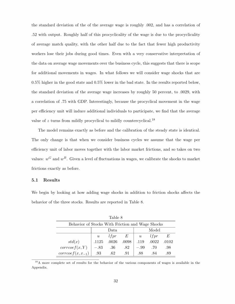
5.1 Results

We begin by looking at how adding wage shocks in addition to friction shocks affects the

behavior of the three stocks. Results are reported in Table 8.

Table 8

Behavior of Stocks With Friction and Wage Shocks

Data Model

u lfpr E u lfpr E

std(x) .1125 .0026 .0098 .119 .0022 .0102

corrcoef(x, Y ) −.83 .36 .82 −.99 .70 .98

corrcoef(x, x−1) .93 .62 .91 .88 .84 .89

18A more complete set of results for the behavior of the various components of wages is available in the

Appendix.

32

As expected, adding wage shocks increases the fluctuations in participation and also serves

to make them more procyclical. This table shows that with modest wage shocks added the

model now accounts for roughly 90 percent of the movements in the participation rate, and

provides almost a perfect match to the volatility of employment. Whereas the model without

wage shocks generated a correlation between participation and output that was marginally

too low, this specification errs on the other side. These results suggest a modest role for wage

movements. Table 9 shows how these wage shocks affect the properties of the gross flows.

The basic patterns are essentially unaffected by the addition of wage shocks, so we do not

spend any additional time on them.

Table 9

Gross Worker Flows in the Data and the Model

A. Abowd-Zellner Adjusted Data

fEU fEN fUE fUN fNE fNU

std(x) .085 .083 .085 .104 .102 .071

corrcoef(x, Y ) −.62 .40 .74 .59 .52 −.20

corrcoef(x, x−1) .55 .29 .74 .60 .38 .29

B. DeNUN ified Data

fEU fEN fUE fUN fNE fNU

std(x) .069 .036 .076 .066 .042 .063

corrcoef(x, Y ) −.66 .29 .81 .55 .57 −.56

corrcoef(x, x−1) .70 .22 .85 .58 .48 .57

C. Model

fEU fEN fUE fUN fNE fNU

std(x) .085 .050 .085 .034 .049 .063

corr(x, Y ) −.85 .16 .75 .89 .55 −.98

corr(x, x−1) .77 .12 .71 .62 .64 .91

While the above results might suggest that cyclical wage movements and their associated

labor supply responses play a modest role, this conclusion is somewhat premature. The

reason for this is that as noted above, our model with on-the-job search and shocks to

frictions implicitly contains an element of procyclical wage movements. Moreover, this effect

is quantitatively important. Although we do not report the details here, when we considered

a similar model that did not allow for on the job search, calibrated in the same fashion, we

33

found that friction shocks alone generated less than half of the fluctuations in the participation

rate. In this sense we think that our model suggests an important role for wage effects on

participation. We conclude that labor supply responses associated with procyclical wage

movements are an important element in accounting for cyclical movements in participation.

6 Conclusion

We have developed a model of individual labor supply in the presence of frictions and used

it to simulate the effects of aggregate shocks to prices and frictions on the labor market

outcomes for of a large set of households. Our key findings are (i) that a model calibrated

to match steady state flows does well in accounting for the cyclical movements of the flows;

(ii) fluctuations in job finding and job loss rates alone do a good job of matching the data,

though this performance involves induced procyclical wage movements through the effects of

frictions wage ladder climbing; and (iii) the labor supply channel is important, despite the

relatively modest, though procyclical, fluctuations in the labor force participation rate. It

is interesting to note, in particular, that as a corollary our model with worker heterogeneity

can match the fluctuations in the participation rate with a rather standard formulation of

household preferences, something which has proved challenging with other setups.

Our model offers a rich yet parsimonious description of individual labor supply in a setting

with heterogeneity, search frictions and an empirically reasonable market structure. It is the

first paper to consider the effects of aggregate shocks on individual labor market transitions in

this setting. However, it is also simplistic in some dimensions relevant for the microeconomic

data. One of these dimensions regards our model of the household as an infinitely-lived

unit. Clearly, an extension that distinguishes different members of the households would be

relevant, as would an age dimension, along the lines of Low, Meghir, and Pistaferri (2010).

We do believe that our framework is a very useful starting point for extensions in various

directions. It can also be used to understand how policy influences labor supply responses,

34

For example, we could use our model to understand how changes in features of the UI system

would influence the labor supply side of the labor market. As one exercise, we have abolished

the UI system in our benchmark model and asked how this affects labor supply responses.

Interestingly, it leads to greater volatility in both the unemployment and employment rates,

as well as in the labor force participation rate.

Related, we also believe that it is useful for assessing a variety of further issues, such as

the heterogeneous effects of business cycles on various subgroups of the population. While

we have focused on aggregate shocks to frictions and the return to market activity, we can

also study other aggregate shocks, including various candidates for demand shocks.

35

References

[1] Abowd, J., and A. Zellner, “Estimating Gross Labor-Force Flows,” Journal of Business

and Economic Statistics 3 (1985), 254-283.

[2] Blanchard, O., and P. Diamond, “The Cyclical Behavior of the Gross Flows of U.S.

Workers,” Brookings Papers on Economic Activity 1990, 85–155.

[3] Card, D., “Intertemporal Labor Supply: An Assessment,” in Advances in Econometrics,

edited by Chris Sims, Cambridge University Press, 1994, 49-81.

[4] Chang, Y., and S. Kim., “From Individual to Aggregate Labor Supply: A Quantita-

tive Analysis Based on a Heterogeneous Agent Macroeconomy,” International Economic

Review 47 (2006), 1–27.

[5] Christiano, L., M. Trabandt, and K. Walentin, “Involuntary Unemployment and the

Business Cycle,” (2010), mimeo.

[6] Chua, T. C. and W. A. Fuller, “A Model for Multinomial Response Error Applier to

Labor Flows,” Journal of the American Statistical Association, (1987) 82, 46–51.

[7] Davis, S.J. and J. Haltiwanger, “Gross Job Creation, Gross Job Destruction, and Em-

ployment Reallocation,” Quarterly Journal of Economics, 107 (1992), 819-863.

[8] Ebell, M., “On the Cyclicality of Unemployment: Resurrecting the Participation Mar-

gin,” Labour Economics 18 (2011), 822–836.

[9] Elsby, M., Hobijn B. and A. Sahin, “On the Importance of the Participation Margin for

Labor Market Fluctuations,” Journal of Monetary Economics, forthcoming, 2015.

[10] Floden, M., and J. Linde, “Idiosyncratic Risk in the United States and Sweden: Is There

a Role for Government Insurance?, Review of Economic Dynamics 4 (2001), 406-437.

36

[11] French, E., “The Effect of Health, Wealth and Wages on Labour Supply and Retirement

Behavior,”Review of Economic Studies 72 (2005), 395-427.

[12] Fujita, S., and G. Ramey, “The Cyclicality of Separation and Job Finding Rates,”

International Economic Review 2 (2009), 415-430.

[13] Galı, J.,“The Return of the Wage Phillips Curve,” Journal of the European Economic

Association, 9 (2011), 436-461.

[14] Galı, J., F. Smets, and R. Wouters, “Unemployment in an Estimated New Keynesian

Model,” mimeo, 2011.

[15] Gertler M., and A. Trigari, “Unemployment Fluctuations with Staggered Nash Wage

Bargaining,” Journal of Political Economy 117 (2009), 38-86.

[16] Haefke, C., and M. Reiter, “What Do Participation Fluctuations Tell Us About Labor

Supply Elasticities?,” Mimeo, IZA, 2011.

[17] Hall, R., “Employment Fluctuations with Equilibrium Wage Stickiness,” American Eco-

nomic Review 95 (2005), 50–65.

[18] Ham, J., “Estimation of a Labour Supply Model with Censoring due to Unemployment

and Underemployment,” Review of Economic Studies XLIX, (1982), 335–354.

[19] Krusell, P., T. Mukoyama, R. Rogerson, and A. Sahin, “Aggregate Labor Market Out-

comes: The Role of Choice and Chance,” Quantitative Economics 1 (2010), 97–128.

[20] Low, A., C. Meghir, and L. Pistaferri, “Wage Risk and Employment Risk over the Life

Cycle,” American Economic Review 100(4) (2010), 1432—1467.

[21] Lucas, R. E., Jr. and Rapping, L. A. “Real Wages, Employment, and Inflation,” Journal

of Political Economy 77(5) (1969), 721-54

37

[22] Mendoza, E., A. Razin, and L. Tesar, “Effective Tax Rates in Macroeconomics: Cross-

Country Estimates of Tax Rates on Factor Incomes and Consumption,” Journal of Mon-

etary Economics 34 (1994), 297-323.

[23] Mortensen, D. T. and C. A. Pissarides, “Job Creation and Job Destruction in the Theory

of Unemployment,” Review of Economic Studies 61 (1994), 397-415.

[24] Poterba, J., and L. Summers, “Reporting Errors and Labor Market Dynamics,” Econo-

metrica 54 (1986), 1319-1338.

[25] Shimer, R., “The Cyclical Behavior of Equilibrium Unemployment and Vacancies,”

American Economic Review, 95:1 (2005), pp. 25–49.

[26] Shimer, R., “Job Search, Labor Force Participation, and Wage Rigidities,” (2011),

mimeo, University of Chicago.

[27] Shimer, R., “Reassessing the Ins and Outs of Unemployment,” Review of Economic

Dynamics, 15:1 (2012), pp. 127–148.

[28] Tjaden, V. and F. Wellschmied, “Quantifying the Contribution of Search to Wage In-

equality,” American Economic Journal: Macroeconomics 6 (2014), 134-161.

[29] Tripier, F., “Can the Labor Market Search Model Explain the Fluctuations of Allocations

of Time?,” Economic Modelling 21 (2004), 131–146.

[30] Veracierto, M., “On the Cyclical Behavior of Employment, Unemployment and Labor

Force Participation,” Journal of Monetary Economics, 55 (2008), 1143–1157.

38

Appendix

A.1 Data

The Current Population Survey (CPS) reports the labor market status of the respondents

each month that allows the BLS to compute important labor market statistics like the unem-

ployment rate. In particular, in any given month a civilian can be in one of three labor force

states: employed (E), unemployed (U), and not in the labor force (N). The BLS definitions

for the three labor market states are as follows:

• An individual is counted as employed if he or she did any work at all for pay or profit

during the survey month. This includes part-time or temporary work as well as full-time

year-round employment.

• An individual is considered unemployed if he or she does not have a job, has actively

looked for employment in the past 4 weeks and is currently available to work.

• An individual is classified as not in the labor force if he or she is included in the labor

force population universe (older than 16 years old, non-military, noninstitutionalized)

but are neither employed nor unemployed.

Households are interviewed for four consecutive months, rotate out for eight months and

then rotate in for another four months. The panel feature of the CPS makes it possible to

calculate transitions by individual workers between these three labor market states. However,

not all the respondents stay in the sample for consecutive months; the rotating feature of the

panel implies that only 75 percent are reinterviewed according to the CPS sampling design.

Moreover, many other respondents cannot be found in the consecutive month due to various

reasons and are reported as missing. The failure to match individuals in consecutive months

is known as margin error and it causes biased estimates of the flow rates as discussed by

Abowd and Zellner (1985), Fujita and Ramey (2009), and Poterba and Summers (1986). The

simplest correction for margin error is to simply drop the missing observations and reweight

39

the transitions that are measured, a procedure that is known as the missing-at-random

(MAR) method. However, this procedure could lead to biases if missing observations are not

missing at random. To deal with this problem, Abowd and Zellner (1985) and Poterba and

Summers (1986) proposed alternative corrections for margin error which use information on

labor market stocks. Their correction reweights the unadjusted flows in order to minimizes

the distance between the reported labor market stocks and the stocks that are imputed

from the labor market transitions. We follow the algorithm proposed by Elsby, Hobijn, and

Sahin (2015), which is similar in spirit to Poterba and Summers’ method, but differs in

implementation. We use the basic monthly CPS files from January 1976 to December 2009.

All transition probabilities are calculated for the population older than 16 years old and are

seasonally adjusted. In addition, we correct for classification error using the estimates of

Abowd and Zellner (1985)which use the reinterview surveys to purge the gross flows data

from classification error. For a detailed discussion of this procedure see Elsby, Hobijn, and

Sahin (2015).

We also compute 95% confidence intervals for various statistics we report related to gross

flows data using bootstrapping. We begin by sampling with replacement 5000 times from

each month of the longitudinally-linked Current Population Survey (CPS) data (each drawn

sample has the same number of observations as the original data), from January 1978 to

December 2009. For each of the 5000 sample data series, we calculate raw flow rates using the

labor status variable and CPS final weights. We then apply the Abowd and Zellner (1985) and

margin adjustment corrections to each sample data series. Finally, we seasonally adjust the

time series of flow rates for each of the 5000 sample series (any month for which a longitudinal

link cannot be made for any observations are linearly interpolated). By computing the

statistics using each of the 5000 series, we are able to construct a distribution of values for

standard deviations, correlations, and autocorrelations. We then report bootstrapped means

and confidence intervals.

40

A.2 Computation

As is described in Section 3.1, the calibration of some parameters of the steady-state

model involves building a simple general equilibrium model in the background. In particular,

we calculate the steady-state values of w, r, and T as the outcome of the general equilibrium

described below. In addition, b is a function of the average wage of the economy, and thus it

is also a fixed-point object.

The general equilibrium structure is very simple. The economy is populated by continuum

of (population one) workers whose decision problem is described in the main text. On the firm

side, there is a representative firm who operates competitively19 with production function

Yt = Kθt L

1−θt ,

where θ is set at .3. Kt =∫aitdi is aggregate input of capital services (which is the sum

of the workers’ assets) and Lt =∫eitzitqitdi is aggregate input of labor services (which is

the sum of the employed workers’ efficiency unit of labor). Output Yt can be used either

for consumption and investment, and capital depreciates at the rate δ = .0067. From the

assumption of the competitive factor market, wt and rt+δ are set at the level of the marginal

products of efficiency unit of labor and capital stock.

The government balances budget every period, that is, it sets the lump-sum transfer Tt

by

Tt =

∫τwteitzitqitdi,

where τ = .30 as we specified in the main text.

One can define a Recursive Competitive Equilibrium of this economy in a standard man-

ner, that is, (i) workers optimize given the prices, (ii) the representative firm optimizes, (iii)

the markets clear, and (iv) the government budget clears.

The computation steps of the Recursive Competitive Equilibrium is as follows.

19One can think of a “island” structure as in Krusell et al. (2011) in order to maintain consistency between

the labor market frictions and the competitive behavior by firms and workers.

41

1. Guess the steady-state level of K/L (which determines w and r), T , and the average

wage.

2. Perform the optimization of the workers.

3. Compute the invariant distribution of the workers over the individual state variables.

4. Compute K/L, T , and the average wage that are implied by the invariant distribution,

and compare with the earlier guess. If they do not coincide, revise the guess and repeat

from Step 2 until convergence.

For the worker optimization (Step 2), we set 48 uneven grids (more grids closer to zero)

over individual capital stock (from a = 0 to a = 1440), 20 grids on z, and 7 grids on q. Both

stochastic processes of z and q are discretized using Tauchen’s (1986) method (the ranges of

the grids are set at two unconditional standard deviations). We have converted the annual

AR(1) process into monthly AR(1) process using the formula analogous to the ones in Chang

and Kim’s (2006) Appendix A.2. In optimization, we have allowed for choosing off-grid values

of at+1 by linearly interpolating the value functions across the grids.

For the computation of the invariant distribution, we represent the distribution of workers

in terms of the “density” (i.e. how many people are at each state) over the state variables

(a, z) in addition to the employment status and UI eligibility. For employed workers, q is an

additional state variable. We iterate the density using the decision rules that were derived in

Step 2 and the Markov transition matrices for stochastic processes until it converges to an

invariant density. In the a direction, we have used a finer set of grids (1000 grids) instead of

the original 48 grids in calculating the density. (The decision rules are linearly interpolated.)

In the economy with shocks, we take the values of r, T , and b as constant. Given the

shocks on λ′s, σ, and w, we can calculate the outcomes in the main texts in the following

two steps.

1. Perform the optimization of the workers.

42

2. Simulate the aggregate behavior using the decision rules from the optimization and the

stochastic processes.

The optimization procedure is similar to the steady-state case. Simulation starts from

the invariant distribution derived in the steady-state model. We simulate the economy for

5000 periods and discard the initial 1000 periods in calculating the statistics.

A.3 Some properties of the model steady state

In this Section, we examine the microeconomic properties of the benchmark model (with-

out aggregate shocks) and compare them to the stylized facts found in microeconomic studies.

First, studies such as Rendon (2006) show that in general employed workers accumulate

asset and nonemployed workers deaccumulate asset. We can see that this is consistent with

the saving behavior of the model agent.

Figure 1: Decision rules for next period asset (net increase), for a given asset level

0 50 100 150 200 250−5

−4

−3

−2

−1

0

1

2

a

a′−a

employed

nonparticipation, eligible

unemployed, ineligible

unemployed, eligible

nonparticipation, ineligible

Figure 1 draws the decision rules (in terms of net increase in asset) for each employment

43

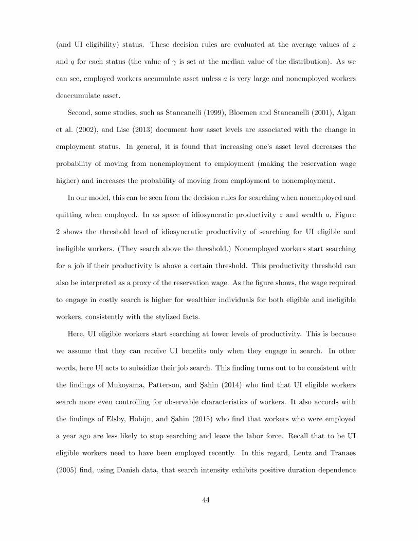
(and UI eligibility) status. These decision rules are evaluated at the average values of z

and q for each status (the value of γ is set at the median value of the distribution). As we

can see, employed workers accumulate asset unless a is very large and nonemployed workers

deaccumulate asset.

Second, some studies, such as Stancanelli (1999), Bloemen and Stancanelli (2001), Algan

et al. (2002), and Lise (2013) document how asset levels are associated with the change in

employment status. In general, it is found that increasing one’s asset level decreases the

probability of moving from nonemployment to employment (making the reservation wage

higher) and increases the probability of moving from employment to nonemployment.

In our model, this can be seen from the decision rules for searching when nonemployed and

quitting when employed. In as space of idiosyncratic productivity z and wealth a, Figure

2 shows the threshold level of idiosyncratic productivity of searching for UI eligible and

ineligible workers. (They search above the threshold.) Nonemployed workers start searching

for a job if their productivity is above a certain threshold. This productivity threshold can

also be interpreted as a proxy of the reservation wage. As the figure shows, the wage required

to engage in costly search is higher for wealthier individuals for both eligible and ineligible

workers, consistently with the stylized facts.

Here, UI eligible workers start searching at lower levels of productivity. This is because

we assume that they can receive UI benefits only when they engage in search. In other

words, here UI acts to subsidize their job search. This finding turns out to be consistent with

the findings of Mukoyama, Patterson, and Sahin (2014) who find that UI eligible workers

search more even controlling for observable characteristics of workers. It also accords with

the findings of Elsby, Hobijn, and Sahin (2015) who find that workers who were employed

a year ago are less likely to stop searching and leave the labor force. Recall that to be UI

eligible workers need to have been employed recently. In this regard, Lentz and Tranaes

(2005) find, using Danish data, that search intensity exhibits positive duration dependence

44

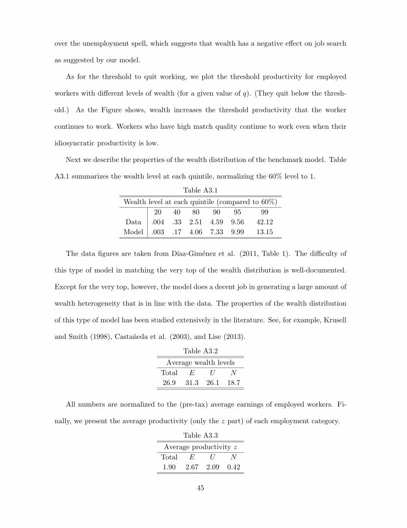
over the unemployment spell, which suggests that wealth has a negative effect on job search

as suggested by our model.

As for the threshold to quit working, we plot the threshold productivity for employed

workers with different levels of wealth (for a given value of q). (They quit below the thresh-

old.) As the Figure shows, wealth increases the threshold productivity that the worker

continues to work. Workers who have high match quality continue to work even when their

idiosyncratic productivity is low.

Next we describe the properties of the wealth distribution of the benchmark model. Table

A3.1 summarizes the wealth level at each quintile, normalizing the 60% level to 1.

Table A3.1

Wealth level at each quintile (compared to 60%)

20 40 80 90 95 99

Data .004 .33 2.51 4.59 9.56 42.12

Model .003 .17 4.06 7.33 9.99 13.15

The data figures are taken from Dıaz-Gimenez et al. (2011, Table 1). The difficulty of

this type of model in matching the very top of the wealth distribution is well-documented.

Except for the very top, however, the model does a decent job in generating a large amount of

wealth heterogeneity that is in line with the data. The properties of the wealth distribution

of this type of model has been studied extensively in the literature. See, for example, Krusell

and Smith (1998), Castaneda et al. (2003), and Lise (2013).

Table A3.2

Average wealth levels

Total E U N

26.9 31.3 26.1 18.7

All numbers are normalized to the (pre-tax) average earnings of employed workers. Fi-

nally, we present the average productivity (only the z part) of each employment category.

Table A3.3

Average productivity z

Total E U N

1.90 2.67 2.09 0.42

45

Figure 2: Upper panel: the threshold level of idiosyncratic productivity of searching for UI

eligible and noneligible workers; lower panel: the threshold level of idiosyncratic productivity

of quitting into nonemployment for UI eligible and noneligible workers—benchmark model.

200 400 600 800 1000 1200 14000

0.5

1

1.5

2

2.5

3

3.5

4

wealth

prod

uctiv

ity

UI eligibleUI noneligible

200 400 600 800 1000 1200 14000

0.5

1

1.5

2

2.5

3

3.5

4

wealth

prod

uctiv

ity

low match qualityhigh math quality

A.4 Additional model properties: wages

There are three components of individual wages: aggregate component wt, individual

productivity zt, and match quality qt. As the composition of employed workers change over

the business cycle, the average values of zt and qt move cyclically.

46

Table A4.1

Behavior of average wages: benchmark model

avg(wzq) w avg(z) avg(q)

std(x) .0018 .0000 .0020 .0008

corrcoef(x, Y ) .52 NA .25 .67

Table A4.1 summarizes the behavior of average wages. (As in the main text, all variables

are aggregated to quarterly, logged, and HP-filtered with the parameter value of 1600.) The

wage per efficiency unit of labor, w, is acyclical by assumption. However, the average wage

per employed worker, avg(wzq), is procyclical. Both average values of z and q are procyclical

and thus contribute to the procyclicality of average wages.

Table A4.2

Behavior of average wages: Section 5

avg(wzq) w avg(z) avg(q)

std(x) .0029 .0025 .0016 .0008

corrcoef(x, Y ) .75 .92 −.28 .60

Table A4.2 summarizes the behavior of the model with wage shocks. With this specifica-

tion, avg(z) is now countercyclical. Both w and avg(q) contributes to the procyclicality of

the average wage per employed worker.

A.5 Model comparison with Great Recession data

In this Section, we look at a specific episode of the Great Recession in light of our model.

Labor force participation rate declined significantly during the Great Recession. A substantial

part of this phenomenon is related to demographic trends, in particular the aging of the U.S.

labor force. The Figure below shows the labor force participation rate starting from 1996,

the year that the share of prime-age workers peaked in the labor force. After 1996, the U.S.

population gradually started to age. A simple way to isolate the effect of aging is to compute

age-adjusted labor force participation rate. First let us define the labor force participation

rate as the weighed average of labor force participation rates of different age groups i where

47

sit is the population share of age group i at time t:

lfprt =∑i

sit × lfprit.

Then let us set the population shares to their values in 1996 and define the age-adjusted

labor force participation rate as

lfprct =∑i

si,1996 × lfprit.

We choose 1996 as our base year since 1996 was the year that the share of prime-age popu-

lation peaked and the share of individuals older than 55 started to increase. Figure 3 shows

that as the baby boom generation moved from their prime ages (the age category with the

highest participation rates) into the older ages, the labor force participation rate has declined;

fixing the population shares at their 1996 levels explains more than 60 percent of the decline

in the labor force participation rate which took place starting in 2008.

Figure 3: Actual and age-adjusted labor force participation rates.

Month

1996 1998 2000 2002 2004 2006 2008 2010 2012 20140.62

0.63

0.64

0.65

0.66

0.67

0.68

1996 1998 2000 2002 2004 2006 2008 2010 2012 20140.62

0.63

0.64

0.65

0.66

0.67

0.68

Labor force participation rate (Left)Age−adjusted labor force participation rate−01/1996 (Left)

Since demographic change is beyond the scope of our paper, we now provide a comparison

of the model’s prediction for a sample recession with the demographically adjusted labor

48

force participation rate in the Great Recession period. In the upper panel of Figure 4, we

normalize the actual and age-adjusted labor force participation rates to their 2007 levels

and plot the change in the 12-month centered average of these rates, along with the change

in the unemployment rate for the 2007–2011 period. We also plot a sample recession from

the simulations of our model in the lower panel of Figure 4. As the model shows, there

is an initial pick-up in participation which reverses rapidly. This is similar to the Great

recession where the participation rate did not start to decline until after the second half of

the recession. In the rest of the sample, the unemployment rate increase is accompanied by

declining participation, quite in line with how it behaved during the Great Recession. Thus,

we think that our model is a promising starting point for thinking about this particular

episode and we plan to pursue this issue more in future work.

49

Figure 4: Upper panel: change in actual and age-adjusted labor force participation rates

and the unemployment rates relative to 2007. Lower panel: labor force participation and

unemployment rates in the model simulation—benchmark model.

Month

2007 2008 2009 2010 2011−0.02

−0.01

0

0.01

2007 2008 2009 2010 2011−0.03

−0.01

0.01

0.03

0.05

0.07

Labor force participation rate (Left)Age−adjusted labor force participation rate−01/1996 (Left)Unemployment Rate (Right)

0 5 10 15 200.67

0.671

0.672

0.673

0.674

0.675

0 5 10 15 200.04

0.05

0.06

0.07

0.08

0.09

Labor force participation rateUnemployment rate

50

Additional References for Appendix

[1] Algan, Y., A. Cheron, J.-O. Hairault, and F. Langot, “Wealth Effect on Labor Market

Transitions,” Review of Economic Dynamics 6 (2002), 156–178.

[2] Bloemen, H., and E. Stancanelli, “Individual Wealth, Reservation Wages, and Transitions

into Employment,” Journal of Labor Economics 19 (2001), 400–439.

[3] Castaneda, A., J. Dıaz-Gimenez, and J.-V. Rıos-Rull, “Accounting for the US Earnings

and Wealth Inequality,” Jouranl of Political Economy 111 (2003), 293–346.

[4] Dıaz-Gimenez, J., A. Glover, and J.-V. Rıos-Rull, “Facts on the Distributions of Earn-

ings, Income, and Wealth in the United States: 2007 Update,” Federal Reserve Bank of

Minneapolis Quarterly Review 34 (2011), 2–31.

[5] Krusell, P., T. Mukoyama, R. Rogerson, and A. Sahin, “A Three State Model of Worker

Flows in General Equilibrium,” Journal of Economic Theory 146 (2011), 1107-1133.

[6] Krusell, P., and A. A. Smith Jr., “Income and Wealth Heterogeneity in the Macroecon-

omy,” Journal of Political Economy 106 (1998), 867–896.

[7] Lentz, R. and T. Tranaes, “Job Search and Savings: Wealth Effects and Duration De-

pendence,” Journal of Labor Economics 23 (2005), 467–489.

[8] Lise, J. “On-the-Job Search and Precautionary Savings,” Review of Economic Studies 80

(2013), 1086–1113.

[9] Mukoyama, T., C. Patterson, and A. Sahin “Job Search Behavior over the Business

Cycle,” (2014). mimeo.

[10] Rendon, S. “Job Search and Asset Accumulation under Borrowing Constraints,” Inter-

national Economic Review 47 (2006), 233–263.

51

[11] Stancanelli, E. “Do the Wealthier Stay Unemployed Longer? An Empirical Study for

the UK,” Oxford Bulletin of Economics and Statistics 61 (1999), 295–314.

[12] Tauchen, G. “Finite State Markov-Chain Approximations to Univariate and Vector Au-

toregressions,” Economics Letters 20 (1986), 177-181.

52