GRNmap Testing

Grace Johnson and Natalie WilliamsJune 3, 2015

GRNmap Testing

• The comparison of estimated weights, production rates, and b values from different runs of the same network will give us insight to further test GRNmap

GRNmap Testing

• Strain Run Comparisons– Each strain alone, two strains, three strains, four strains, all

strains• Non-1 Initial Weights Comparisons

– Initial weights = 0– Initial weights = 1– Initial weights = -1– Initial weights = 3– Initial weights = -3– Initial weights = 10– Three runs with weights randomly distributed between -1 and 1– One run with weights randomly distributed between -3 and 3

To compare estimated parameters we ran GRNmap using data from:

• Wt alone• Each deletion strain alone• Wt vs each deletion strain• Wt + dCIN5 + dZAP1• Wt + dCIN5 + dZAP1 + dGLN3

Estimated production rates and b values varied widely between strain runs

Figure 1: Estimated b values

Figure 2: Estimated production rates

Estimated weights also varied widely between strain runs

Figure 3: regulator PHD1 Figure 4: regulator SKN7

Figure 6: regulator CIN5Figure 5: regulator FHL1

Figure 7: Unweighted network

Figure 9: All strains, initial weights 1

Figure 8: wt only, initial weights 1

Visualized networks also display variations between runs

All-strain, varied weight comparisons

• The purpose of this test is to see how model outputs for the same network are affected by different initial weight guesses (other than 1). We evaluate by looking at LSE values and estimated parameters.– We did not further analyze one-strain runs

because they exhibited no difference when initial weights were varied

Figure 10: Estimated b values

Figure 11: Estimated production rates

Estimated production rates and b values remained relatively consistent with different weights

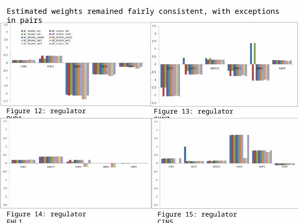
Figure 12: regulator PHD1 Figure 13: regulator SKN7

Figure 15: regulator CIN5Figure 14: regulator FHL1

Estimated weights remained fairly consistent, with exceptions in pairs

Figure 16: All strains, initial weights 1

Figure 17: All strains, initial weights 0

Visualized networks showed slight differences

LSE’s of outputs with different weights show the same three groupings

Run All Strains Wt Only

w = -1 45.2566 N/A

w = -3 45.2565 N/A

w =1 45.7010 6.8824

w = 3 45.6978 6.8824

w = 0 45.3083 6.8824

w = 10 45.3083 N/A

w = rand (-1,1) 45.3083 6.8824

w = rand (-1,1) 45.3083 N/A

w = rand (-1,1) 45.3083 N/A

w = rand (-3,3) 45.3083 N/A

Ideal LSE (sum of squares) 0.5520 0.4875

Figure 18 : Output LSE values

As the number of strains analyzed increases, the code output LSE displays a linear trend