grid-free compressive beamforming...grid-free compressive beamforming angeliki xenakia) department...

General rights Copyright and moral rights for the publications made accessible in the public portal are retained by the authors and/or other copyright owners and it is a condition of accessing publications that users recognise and abide by the legal requirements associated with these rights.

Users may download and print one copy of any publication from the public portal for the purpose of private study or research.

You may not further distribute the material or use it for any profit-making activity or commercial gain

You may freely distribute the URL identifying the publication in the public portal If you believe that this document breaches copyright please contact us providing details, and we will remove access to the work immediately and investigate your claim.

Downloaded from orbit.dtu.dk on: Mar 09, 2020

Grid-free compressive beamforming

Xenaki, Angeliki; Gerstoft, Peter

Published in:Acoustical Society of America. Journal

Link to article, DOI:10.1121/1.4916269

Publication date:2015

Document VersionPublisher's PDF, also known as Version of record

Link back to DTU Orbit

Citation (APA):Xenaki, A., & Gerstoft, P. (2015). Grid-free compressive beamforming. Acoustical Society of America. Journal,137(4), 1923-1935. https://doi.org/10.1121/1.4916269

https://doi.org/10.1121/1.4916269

https://orbit.dtu.dk/en/publications/8445c3d3-8962-44ee-9058-45a18ceda279

https://doi.org/10.1121/1.4916269

Grid-free compressive beamforming

Angeliki Xenakia)

Department of Applied Mathematics and Computer Science, Technical University of Denmark, Kgs. Lyngby2800, Denmark

Peter GerstoftScripps Institution of Oceanography, University of California San Diego, La Jolla, California 92093-0238

(Received 5 November 2014; revised 3 February 2015; accepted 2 March 2015)

The direction-of-arrival (DOA) estimation problem involves the localization of a few sources from

a limited number of observations on an array of sensors, thus it can be formulated as a sparse signal

reconstruction problem and solved efficiently with compressive sensing (CS) to achieve high-

resolution imaging. On a discrete angular grid, the CS reconstruction degrades due to basis mis-

match when the DOAs do not coincide with the angular directions on the grid. To overcome this

limitation, a continuous formulation of the DOA problem is employed and an optimization proce-

dure is introduced, which promotes sparsity on a continuous optimization variable. The DOA esti-

mation problem with infinitely many unknowns, i.e., source locations and amplitudes, is solved

over a few optimization variables with semidefinite programming. The grid-free CS reconstruction

provides high-resolution imaging even with non-uniform arrays, single-snapshot data and under

noisy conditions as demonstrated on experimental towed array data.VC 2015 Acoustical Society of America. [http://dx.doi.org/10.1121/1.4916269]

[ZHM] Pages: 1923–1935

I. INTRODUCTION

Sound source localization with sensor arrays involves

the estimation of the direction-of-arrival (DOA) of (usually a

few) sources from a limited number of observations.

Compressive sensing1,2 (CS) is a method for solving such

underdetermined problems with a convex optimization pro-

cedure which promotes sparse solutions.

Solving the DOA estimation as a sparse signal recon-

struction problem with CS, results in robust, high-resolution

acoustic imaging,3–6 outperforming traditional methods7 for

DOA estimation. Furthermore, in ocean acoustics, CS is

shown to improve the performance of matched field process-

ing,8,9 which is a generalized beamforming method for local-

izing sources in complex environments (e.g., shallow water),

and of coherent passive fathometry in inferring the number

and depth of sediment layer interfaces.10

One of the limitations of CS in DOA estimation is basis

mismatch11 which occurs when the sources do not coincide

with the look directions due to inadequate discretization of

the angular spectrum. Under basis mismatch, spectral leak-

age leads to inaccurate reconstruction, i.e., estimated DOAs

deviating from the actual ones. Employing finer grids3,12

alleviates basis mismatch at the expense of increased compu-

tational complexity, especially in large two-dimensional or

three-dimensional problems as encountered in seismic imag-

ing, for example.13–15

To overcome basis mismatch, we formulate the DOA

estimation problem in a continuous angular spectrum and

introduce a sparsity promoting measure for general signals,

the atomic norm.16 The atomic norm minimization problem,

which has infinitely many unknowns, is solved efficiently

over few optimization variables in the dual domain with

semidefinite programming.17 Utilizing the dual optimal vari-

ables, we show that the DOAs are accurately reconstructed

through polynomial rooting. It is demonstrated that grid-free

CS gives robust, high-resolution reconstruction also with

non-uniform arrays and noisy measurements, exhibiting

great flexibility in practical applications.

Polynomial rooting is employed in several DOA estima-

tion methods to improve the resolution. However, these

methods involve the estimation of the cross-spectral matrix

hence they require many snapshots and stationary incoherent

sources and are suitable only for uniform linear arrays

(ULA).18 Grid-free CS is demonstrated not to have these

limitations.

Finally, we process acoustic data19 from measurements

in the North-East (NE) Pacific with grid-free CS and demon-

strate that the method provides high-resolution acoustic

imaging even with single-snapshot data.

In this paper, vectors are represented by bold lowercase

letters and matrices by bold uppercase letters. The symbolsT , H denote the transpose and the Hermitian (i.e., conjugate

transpose) operator, respectively, on vectors and matrices.

The symbol � denotes simple conjugation. The generalized

inequality X � 0 denotes that the matrix X is positive semi-

definite. The ‘p-norm of a vector x 2 Cn

is defined as

kxkp ¼ ðPn

i¼1 jxijpÞ1=p. By extension, the ‘0-norm is defined

as kxk0 ¼Pn

i¼1 1xi 6¼0. The paper makes heavy use of convex

optimization theory; for a summary see Appendix A.

II. DISCRETE DOA ESTIMATION

The DOA estimation problem involves the localization

of usually a few sources from measurements on an array of

a)Author to whom correspondence should be addressed. Electronic mail:

[email protected]

J. Acoust. Soc. Am. 137 (4), April 2015 VC 2015 Acoustical Society of America 19230001-4966/2015/137(4)/1923/13/$30.00

http://dx.doi.org/10.1121/1.4916269

mailto:[email protected]

http://crossmark.crossref.org/dialog/?doi=10.1121/1.4916269&domain=pdf&date_stamp=2015-04-01

sensors. For simplicity, we assume that the sources are in the

far-field of the array, such that the wavefield impinging on

the array consists of a superposition of plane waves, that the

processing is narrowband and the sound speed is known.

Moreover, we consider the one-dimensional problem with a

uniform linear array of sensors and the sources residing in

the plane of the array.

The location of a source is characterized by the direction

of arrival of the associated plane wave, h 2 ½�908; 908�,with respect to the array axis. The propagation delay from

the ith potential source to each of the M array sensors is

described by the steering (or replica) vector

aðhiÞ ¼ ej2pðd=kÞ½0;…;M�1�T sin hi ; (1)

where k is the wavelength and d is the intersensor spacing.

Discretizing the half-space of interest, h 2 ½�908; 908�,into N angular directions the DOA estimation problem is

expressed in a matrix-vector formulation

y ¼ Ax; (2)

where y 2 CM is the vector of the wavefield measurements

at the M sensors, x 2 CN

is the unknown vector of the com-

plex source amplitudes at all N directions on the angular grid

of interest, and A is the sensing matrix which maps the sig-

nal to the observations

AM�N ¼ ½aðh1Þ;…; aðhNÞ�: (3)

In the presence of additive noise n 2 CM

, the measurement

vector is described by

y ¼ Axþ n: (4)

The noise is generated as independent and identically distrib-

uted complex Gaussian. The array signal-to-noise ratio

(SNR) for a single-snapshot is used in the simulations,

defined as SNR¼ 20 log10ðkAxk2=knk2Þ, which determines

the noise ‘2-norm, knk2 ¼ kAxk210�SNR=20.

A. Sparse signal reconstruction

Practically, we are interested in a fine resolution on the

angular grid such that M < N and problem (2) is underdeter-

mined. A way to solve this ill-posed problem is to constrain

the possible solutions with prior information.

Traditional methods solve the underdetermined problem

(2) by seeking the solution with the minimum ‘2-norm which

fits the data as described by the minimization problem

minx2C

Nkxk2 subject to y ¼ Ax: (5)

The minimization problem (5) is convex with analytic solu-

tion, x ¼ AHðAAHÞ�1y. However, it aims to minimize the

energy of the signal rather than its sparsity, hence the result-

ing solution is non-sparse.

Conventional beamforming20 (CBF) is the simplest

source localization method and it is based on the ‘2-norm

method with the simplifying condition AAH ¼ IM. CBF

combines the sensor outputs coherently to enhance the signal

at a specific look direction from the ubiquitous noise yield-

ing the solution

xCBF ¼ AHy: (6)

CBF is robust to noise but suffers from low resolution and

the presence of sidelobes.

A sparse solution x is preferred by minimizing the ‘0-

norm leading to the minimization problem

minx2C

Nkxk0 subject to y ¼ Ax: (7)

However, the minimization problem (7) is a non-convex

combinatorial problem which becomes computationally in-

tractable even for moderate dimensions. The breakthrough

of compressive sensing1,2 (CS) came with the proof that for

sufficiently sparse signals, K � N, K < M, and sensing mat-

rices with sufficiently incoherent columns the minimization

problem (7) is equivalent to the minimization problem

minx2C

Nkxk1 subject to y ¼ Ax; (8)

where the ‘0-norm is replaced with the ‘1-norm. The prob-

lem (8) is the closest convex optimization problem to prob-

lem (7) and can be solved efficiently by convex optimization

even for large dimensions.21

For noisy measurements Eq. (4), the constraint in Eq.

(8) becomes ky� Axk2 � �, where � is the noise floor, i.e.,

knk2 � �. Then, the solution is22

xCS ¼ argminx2C

N

kxk1 subject to ky� Axk2 � �; (9)

which has the minimum ‘1-norm while it fits the data up to

the noise level.

Herein, we use the cvx toolbox for disciplined convex

optimization which is available in the Matlab environment.

It uses interior point solvers to obtain the global solution of a

well-defined optimization problem.23 Interior point methods

solve an optimization problem with linear equality and in-

equality constraints by transforming it to a sequence of sim-

pler linear equality constrained problems which are solved

iteratively with the Newton’s method (iterative gradient

descent method) increasing the accuracy of approximation at

each step.24

B. Basis mismatch

CS offers improved resolution due to the sparsity con-

straint and it can be solved efficiently with convex optimiza-

tion. However, CS performance in DOA estimation is limited

by the coherence of the sensing matrix A (see Ref. 5),

described by the restricted isometry property,25 and by basis

mismatch11,12 due to inadequate discretization of the angular

grid. Herein, we demonstrate a way to overcome the limita-

tion of basis mismatch by solving the ‘1-minimization prob-

lem on a grid-free, continuous spatial domain.

1924 J. Acoust. Soc. Am., Vol. 137, No. 4, April 2015 A. Xenaki and P. Gerstoft: Grid-free compressive beamforming

The fundamental assumption in CS is the sparsity of the

underlying signal in the basis of representation, i.e., the sens-

ing matrix A. However, when the sources do not match with

the selected angular grid, the signal might not appear sparse

in the selected discrete Fourier transform basis.11 Figure 1

shows the degradation of CS performance under basis mis-

match due to inadequate discretization of the DOA domain

in fast Fourier transform beamforming.

To increase the precision of the CS reconstruction,

Malioutov et al.3 and Duarte and Baraniuk12 propose an

adaptive grid refinement. The adaptive grid refinement aims

at improving the resolution of CS reconstruction without sig-

nificant increase in the computational complexity by first

detecting the regions where sources are present on a coarse

grid and then refining the grid locally only at these regions.

Grid refinement is an intuitive way of circumventing basis

mismatch. However, the problem of basis mismatch is

avoided only if the problem is solved in a continuous setting,

particularly for moving sources.

III. CONTINUOUS DOA ESTIMATION

In the continuous approach, the K-sparse signal, x, is

expressed as

xðtÞ ¼XK

i¼1

xidðt� tiÞ; (10)

where xi 2 C is the complex amplitude of the ith source,

ti ¼ sin hi is its support, i.e, the corresponding DOA, on the

continuous sine spectrum T ¼ ½�1; 1� (with T T the set

of the DOAs of all K sources) and dðtÞ is the Dirac delta

function.

The sound pressure received at the mth sensor is

expressed as a superposition of plane waves from all possi-

ble directions on the continuous sine spectrum T,

ym¼ð1

�1

xðtÞej2pðd=kÞðm�1Þtdt¼XK

i¼1

xiej2pðd=kÞðm�1Þti ; (11)

and the measurement vector of the sensor array is

yM�1 ¼ FMx; (12)

where FM is a linear operator (inverse Fourier transform)

which maps the continuous signal x to the observations

y 2 CM

.

In the presence of additive noise, n 2 CM, the measure-

ment vector is described by

y ¼ FMxþ n; (13)

similarly to Eq. (4).

IV. GRID-FREE SPARSE RECONSTRUCTION

To solve the underdetermined problem (12) [or equiva-

lently problem (13)] in favor of sparse solutions, we describe

an optimization procedure which promotes sparsity on a con-

tinuous optimization variable.

A. Atomic norm

In the discrete formulation (4) of the DOA estimation

problem, the prior information about the sparse distribution

of sources is imposed through the ‘1-norm of the vector x to

obtain sparse estimates (9). By extension, in the continuous

formulation (13), we introduce the atomic norm,16 k kA, as

a sparsity promoting measure for the continuous signal xðtÞin Eq. (10) defined as

kxkA ¼XK

i¼1

jxij: (14)

In other words, the atomic norm is a measure for continuous

signals equivalent to the ‘1-norm (which is defined only on

vector spaces). Hence, the atomic norm is a convex function

which promotes sparsity in a general framework. For a dis-

crete grid the atomic norm corresponds to the ‘1-norm.

To clarify the analogy between the ‘1-norm and the

atomic norm and justify the term atomic, consider that the

vector x 2 CN

can be interpreted as a linear combination of

N unit vectors. The unit vectors, in this case, are the smallest

units, or atoms, in which the vector x can be decomposed

into. The ‘1-norm is the sum of the absolute values of the

weights of this linear combination of atoms.24

Analogously, the continuous signal (10) can be interpreted

as a linear combination of K delta functions dðt� tiÞ, serving

as atoms for the continuous signal xðtÞ and the atomic norm is

the sum of the absolute values of the weights of the linear

combination of these atoms.16 Even though there are infinitely

many atoms in the continuous case, only few of those, K < M,

constitute the signal and the sum in Eq. (14) is finite.

B. Primal problem

Utilizing the convex measure of the atomic norm, the

DOA estimation in the continuous angular space is solved

with the sparsity promoting minimization problem,

minxkxkA subject to y ¼ FMx: (15)

Since the optimization variable x is a continuous parame-

ter, the primal problem (15) is infinite dimensional and cannot

be solved as such. It is possible to approximate the continuous

variable x on a discrete grid and solve the ‘1-norm optimiza-

tion problem (8). This would increase the computational

FIG. 1. (Color online) CS performance in DOA estimation in terms of the

discretization of the angular space. A standard ULA is used with M¼ 8 sen-

sors, d=k ¼ 1=2 and SNR¼ 20 dB. CBF and CS (*) reconstruction of two

sources (o) (a) at 08 and 158 on a grid ½�908 : 58 : 908�, (b) at 08 and 178 on

a grid ½�908 : 58 : 908�, and (c) at 08 and 178 on a grid ½�908 : 18 : 908�.

J. Acoust. Soc. Am., Vol. 137, No. 4, April 2015 A. Xenaki and P. Gerstoft: Grid-free compressive beamforming 1925

complexity significantly when the discretization step is

reduced to improve precision. An alternative to this, is to grad-

ually refine the discretization step.3 However, we show that by

solving the dual problem instead, there is no need to employ a

discrete approximation of the continuous variable, x.

C. Dual problem

To formulate the dual problem to problem (15) (see

Appendix A for details), we construct the Lagrangian by

making the explicit equality constraints, y ¼ FMx, implicit

in the objective function,

Lðx; cÞ ¼ kxkA þ Re½cHðy� FMxÞ�; (16)

where c 2 CM is the vector of dual variables.

The dual function gðcÞ is the infimum, i.e., the greatest

lower bound, of the Lagrangian, Lðx; cÞ, over the primal

optimization variable x,

gðcÞ ¼ infx

Lðx; cÞ

¼ Re½cHy� þ infxðkxkA � Re½cHFM x�Þ: (17)

To evaluate the second term in Eq. (17) we note that for ev-

ery xi, Re½ðcHFMÞixi� ¼ Re½ðFHMcÞHi xi� ¼ jðFH

McÞijjxij cos /i,

where /i is the angle between xi and ðFHMcÞi. Then,

jxij � Re½ðFHMcÞHi xi� ¼ jxij½1� jðFH

McÞij cos /i�� jxij½1� jðFH

McÞij�: (18)

The lower bound in Eq. (18) is non-negative if jFHMcj is less

than one, maxijðFHMcÞij � 1, and the infimum is zero.

Otherwise, jxij½1� jðFHMcÞij� < 0 and the infimum is

attained at �1. Hence, the dual function is

gðcÞ ¼ Re½cHy�; kFHMck1 � 1

�1; otherwise:

((19)

From Eq. (18), jxij½1� jðFHMcÞij cos /i� ¼ 0 at the infi-

mum, which for every xi 6¼ 0 yields jðFHMcÞij cos /i ¼ 1, i.e.,

jðcHFMÞij ¼ 1 and /i ¼ 0, as both jðcHFMÞij � 1 and

cos /i � 1. Thus, for xi 6¼ 0, ðFHMcÞi is a unit vector in the

direction of xi,

ðFHMcÞi ¼ xi=jxij; xi 6¼ 0;

jFHMcij < 1; xi ¼ 0: (20)

Maximizing the dual function (19) constitutes the dual

problem

maxc2C

MRe½cHy� subject to kFH

Mck1 � 1: (21)

Since the primal problem (15) is convex with linear equality

constraints (A11), strong duality holds assuring that the max-

imum of the dual problem (21) is equal to the minimum of

the primal problem.

The dual problem (21) selects a vector c 2 CM

which is

maximally aligned with the measurement vector y 2 CM

while

its beamformed amplitude jFHMcj is bounded by unity across

the whole angular spectrum. At the angular direction corre-

sponding to the DOA of an existing source, the beamformed

dual vector (20) is equal to the normalized source amplitude.

D. Dual problem using semidefinite programming

The dual problem (21) is a semi-infinite programming

problem with a finite number of optimization variables,

c 2 CM

, and infinitely many inequality constraints, which is

still intractable.

Define the dual polynomial

HðzÞ ¼ FHMc ¼

XM�1

m¼0

cmzm ¼XM�1

m¼0

cme�j½2pðd=kÞt�m: (22)

Note that FHMc is a trigonometric polynomial (B1), of the

variable zðtÞ ¼ e�j2pðd=kÞt, t 2 T, with the dual variables c

¼ ½c0;…; cM�1�T as coefficients and degree M � 1.

The inequality constraint in Eq. (21) implies that the

dual polynomial has amplitude uniformly bounded for all

t 2 T; see Eq. (B7). Making use of the approximation in Eq.

(B6) for bounded trigonometric polynomials, the constraint

in Eq. (21) can be replaced with finite dimensional linear

matrix inequalities. Thus, the dual problem is solved with

semidefinite programming,23,24 i.e., a convex optimization

problem where the inequality constraints are linear matrix

inequalities with semidefinite matrices

maxc;Q

ReðcHyÞ subject to

�QM�M cM�1

cH1�M 1

�� 0;

XM�j

i¼1

Qi;iþj ¼(

1; j ¼ 0

0; j ¼ 1; :::;M � 1:(23)

The number of optimization variables of the dual prob-

lem (23) is ðM þ 1Þ2=2 equal to half the number of elements

of the Hermitian matrix in the inequality constraint. Thus, a

problem with infinitely many unknown parameters, Eq. (15),

is solved over a few optimization variables.

E. Support detection through the dual polynomial

Strong duality assures that by solving the dual problem

(21), or equivalently Eq. (23), we obtain the minimum of the

primal problem (15). However, the dual problem provides an

optimal dual vector, c, but not the primal solution, x. Since

the corresponding dual polynomial, HðzÞ ¼ FHMc; has the

properties in Eq. (20), the support T of the primal solution xcan be estimated by locating the angular directions ti where

the amplitude of the dual polynomial is one (i.e., the angular

directions at the maxima of the beamformed dual vector),

jHðzÞj � 1; 8t 2 T! jH½zðtiÞ�j ¼ 1; ti 2 T

jH½zðtÞ�j < 1; t 2 TnT :

(

(24)

Following Appendix B 4, this is done by locating the

roots of the non-negative polynomial which lie on the unit

circle jzj ¼ 1 (see also Sec. VIII B),


PðzÞ ¼ 1� RðzÞ ¼ 1�XM�1

m¼�ðM�1Þrmzm; (25)

where RðzÞ ¼ HðzÞHðzÞH ¼ jHðzÞj2 with coefficients rm

¼PM�1�m

l¼0 clc�lþm, m � 0 and r�m ¼ r�m, i.e., the autocorre-

lation of c.

Note that the polynomial of degree 2ðM � 1Þ,

PþðzÞ ¼ zM�1PðzÞ ¼ ð1� r0ÞzM�1

�XM�1

m¼�ðM�1Þ;m 6¼0

rmzðmþM�1Þ; (26)

which has only positive powers of the variable z, has the

same roots as PðzÞ, besides the trivial root z ¼ 0. Thus, the

support T of x, i.e., the DOAs of the sources, is recovered by

locating the roots of PþðzÞ on the unit circle (see Fig. 2),

T ¼ ti ¼k

2pdarg zi jPþ zið Þ ¼ 0; jzij ¼ 1

� �: (27)

F. Reconstruction of the primal solution x

Once the support is recovered by locating the roots of

the polynomial in Eq. (26) that lie on the unit circle (27), the

source amplitudes [the complex weights in Eq. (10)] are

recovered from

xCSdual¼ AþT y; (28)

where þ denotes the pseudoinverse of AT with columns

aðtiÞ ¼ ej2pðd=kÞ½0;…;M�1�T ti for ti 2 T .

Figure 3 shows the DOA estimation with grid-free CS

following the procedure described in this section (see

Appendix C for a MATLAB implementation). The dual polyno-

mial attains unit amplitude, jHðzÞj ¼ 1, at the support of the

solution, i.e., the DOAs of the existing sources; see Fig. 3(a).

Figure 3(b) compares the grid-free CS (28) and the CBF

reconstruction in DOA estimation. The grid-free CS offers

very accurate localization, while CBF is characterized by

low resolution. Moreover, CBF fails to detect the weak

source at 15:9628 since it is totally masked by the sidelobes.

V. MAXIMUM RESOLVABLE DOAS

The maximum number of resolvable DOAs with grid-

free CS is determined by the maximum number of roots of

PþðzÞ in Eq. (26) which can be on the unit circle, jzj ¼ 1.

Since the coefficients of the polynomial PþðzÞ are conjugate

symmetric around the term zM�1, the roots appear in pairs at

the same angular direction tl, one inside the unit circle, zin

¼ rle�j2pðd=kÞ tl at radius rl < 1, and the other outside of the

unit circle zout ¼ ð1=rlÞe�j2pðd=kÞ tl ¼ 1=ðzinÞH . This implies

that the roots on the unit circle have double multiplicity. The

polynomial PþðzÞ has in total 2ðM � 1Þ roots, as determined

by its degree. Hence, there are at most M � 1 (double) roots

on the unit circle.

The necessary condition for the dual polynomial (24) to

satisfy the condition jHðzÞj < 1 for some t 2 T, thus avoid

the non-informative case of a constant dual polynomial, is

that the number of sources should not exceed17,26

Kmax ¼M � 1

2

� �; (29)

where bc is the largest integer not greater than the argument.

In other words, at least half of the (paired) M � 1 roots

should lie off the unit circle alternating with the roots on the

unit circle leading to the bound (29).

For positive source amplitudes, xi 2 Rþ, the condition

(29) is sufficient and no separation condition is required for

the resolvable sources.26 However, for complex amplitudes,

xi 2 C, the sources are resolved uniquely only if the corre-

sponding DOAs are separated by at least,17,27

minti; tj2T

jti � tjj ¼k

Md; (30)

where jti � tjj is a wrap-around distance meaning that we

identify the points �1, 1, in T ¼ ½�1; 1�.

FIG. 2. (Color online) Support detection through the dual polynomial. A ULA

is used with M ¼ 21 sensors and d=k ¼ 1=2 to localize three sources with sup-

port set T ¼ ½�0:126; 0:275; 0:67�. (a) The dual polynomial jHðzÞj. (b) The

non-negative polynomial PðzÞ. (c) The support T is estimated by the angle of

the roots, zi, of PðzÞ for which jzij ¼ 1.

FIG. 3. (Color online) Grid-free sparse reconstruction. A standard ULA is

used with M ¼ 21 sensors and d=k ¼ 1=2 to localize three sources (�) at h¼ ½�7:23858; 15:9628; 42:06718� with amplitudes jxj ¼ ½1; 0:01; 0:6�. (a)

The dual polynomial. (b) Reconstruction with grid-free CS (*) and CBF.


The minimum separation condition (30) is a consequence

of the coherence of the sensing process which is related to the

beampattern; see Sec. IV D in Ref. 5. To guarantee a well-

posed sparse signal reconstruction, it is required that the col-

umns of the inverse Fourier operator FM, the steering vectors

(1), are sufficiently uncorrelated. The continuous formulation

(12) implies that adjacent steering vectors are in arbitrarily

close directions, hence fully coherent. However, the require-

ment (30) inhibits closely spaced (i.e., highly correlated)

steering vectors, hence prevents the sparse reconstruction

problem from being too ill-posed due to coherence.

Figure 4 shows the reconstruction for the maximum

number of sources possible. For positive source amplitudes,

xi 2 Rþ, the bound (29) suffices to ensure a unique solution.

Grid-free CS achieves super-resolution even for DOAs in

general position; see Figs. 4(a)–4(b). Inserting an additional

source at 71:818, thus exceeding the maximum number of

resolvable sources (29), results in a non-informative dual

polynomial, jHðzÞj � 1, for all t 2 T, Fig. 4(c), and inaccu-

rate reconstruction where only seven out of the 11 sources

are resolved, Fig. 4(d). For complex source amplitudes,

xi 2 C, an additional constraint (30) on the minimum

separation of DOAs is required along with the bound on the

number of sources (29) to ensure a unique solution, Figs.

4(e)–4(f). Violating the minimum separation condition, the

CS DOA estimation becomes extremely ill-posed due to the

coherence of the underlying steering vectors resulting in

inaccurate reconstruction characterized by the presence of

spurious sources, Figs. 4(g)–4(h).

VI. NON-UNIFORM ARRAYS

The method is also applicable to non-uniform arrays,

constructed by randomly choosing sensors from a standard

ULA configuration, by adding an additional constraint in the

optimization problem (23).27 The additional constraint

ensures that coefficients of the dual polynomial correspond-

ing to inactive sensors on the ULA, cmnull, are annihilated.

The dual problem in a semidefinite programming formu-

lation (23) is augmented with an additional constraint and

takes the form

maxc;Q

ReðcHyÞ subject toQM�M cM�1

cH1�M 1

" #� 0;

XM�j

i¼1

Qi;iþj ¼1; j ¼ 0

0; j ¼ 1; :::;M� 1; cmnull

¼ 0:

((31)

Figure 5 shows the DOA estimation with grid-free CS

and compares it with the CBF reconstruction in the case of a

random array. Even though CBF performance degrades sig-

nificantly due to the increased sidelobe levels introduced by

the random array and the strong source towards endfire, CS

still offers exact reconstruction.

VII. GRID-FREE RECONSTRUCTION WITH NOISE

The problem of grid-free DOA estimation with CS

extends to noisy measurements making the framework useful

for practical applications. Assuming that the measurements

[Eq. (13)] are contaminated with additive noise n 2 CM,

such that knk2 � �, the atomic norm minimization problem

(15) is reformulated as28

FIG. 4. (Color online) Grid-free sparse reconstruction. A ULA is used with

M ¼ 21 sensors and d=k ¼ 1=2 to localize the possible maximum number of

sources (�), bðM � 1Þ=2c ¼ 10. (a) The dual polynomial and (b) reconstruc-

tion with grid-free CS (*) and CBF for sources with positive amplitudes,

x10;R ¼ ½0:8; 0:6; 0:9; 0:5; 1; 0:9; 0:1; 1; 0:4; 0:7�. (c) The dual polynomial

and (d) reconstruction for 11 sources with positive amplitudes, x11;R

¼ ½x10;R; 0:1�. (e) The dual polynomial and (f) reconstruction for sources

with complex amplitudes, x10; C ¼ x10; R þi½�1:6; 0:5; �1:3; �2:6; 0:4;�1:2; �1:2; �0:6; �0:5; 0:6�, separated by the condition (30). (g) The dual

polynomial and (h) reconstruction for sources with complex amplitudes,

x10; C, but locations violating the condition (30).

FIG. 5. (Color online) Grid-free sparse reconstruction. (a) A random array

constructed by randomly selecting M ¼ 13 sensors out of a standard ULA

with 21 sensors and d=k ¼ 1=2. The sources (�) are at h ¼ ½�32:88818;25:27738; 69:39038� with amplitudes jxj ¼ ½0:67; 0:33; 1�. (b) The dual

polynomial. (c) Reconstruction with grid-free CS (*) and CBF.


minxkxkA subject to ky� FMxk2 � �: (32)

To solve the infinite dimensional primal problem (32) we

formulate the equivalent dual problem (see Appendix D)

maxc

ReðcHyÞ � �kck2 subject to kFHMck1 � 1; (33)

and we replace the infinite-dimensional constraints with fi-

nite matrix inequalities,

maxc;Q

ReðcHyÞ � �kck2 subject toQM�M cM�1

cH1�M 1

" #� 0;

XM�j

i¼1

Qi;iþj ¼1; j ¼ 0

0; j ¼ 1; :::;M� 1:

((34)

Problem (34) is a convex optimization problem which

can be solved efficiently with semidefinite programming23 to

obtain an estimate for the coefficients, c 2 CM

, of the dual

polynomial. The support of the solution, i.e., the DOAs of

the existing sources is found by locating the points where the

dual polynomial has unit amplitude following the methodol-

ogy in Sec. IV E. Once the support is recovered the source

amplitudes are estimated by solving a discrete overdeter-

mined problem, Eq. (28).

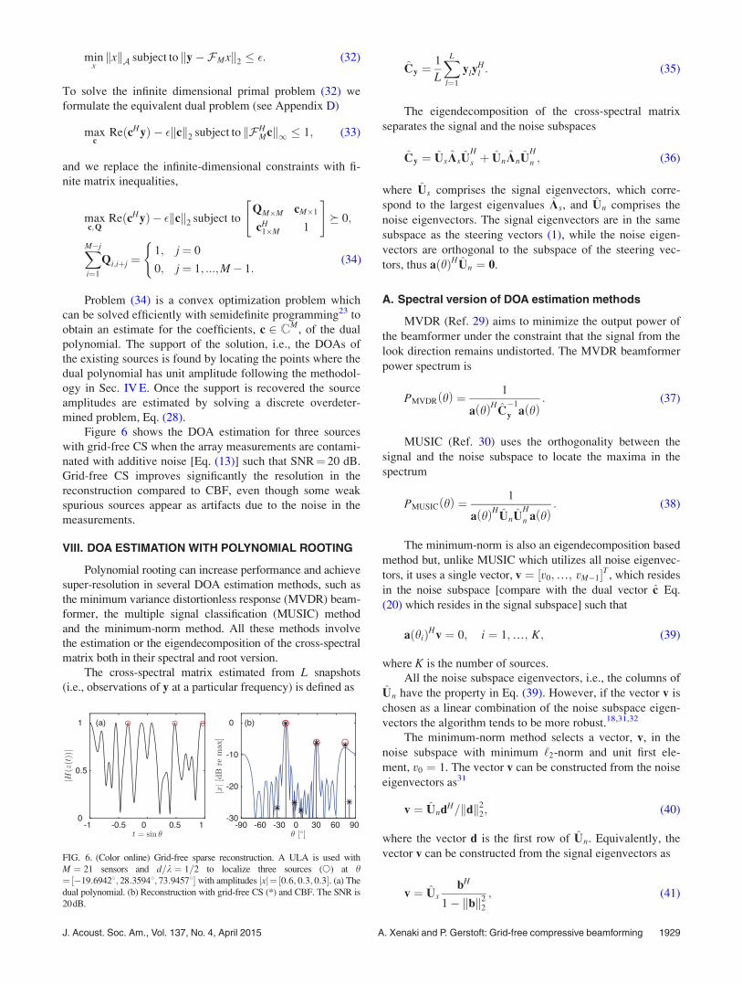
Figure 6 shows the DOA estimation for three sources

with grid-free CS when the array measurements are contami-

nated with additive noise [Eq. (13)] such that SNR¼ 20 dB.

Grid-free CS improves significantly the resolution in the

reconstruction compared to CBF, even though some weak

spurious sources appear as artifacts due to the noise in the

measurements.

VIII. DOA ESTIMATION WITH POLYNOMIAL ROOTING

Polynomial rooting can increase performance and achieve

super-resolution in several DOA estimation methods, such as

the minimum variance distortionless response (MVDR) beam-

former, the multiple signal classification (MUSIC) method

and the minimum-norm method. All these methods involve

the estimation or the eigendecomposition of the cross-spectral

matrix both in their spectral and root version.

The cross-spectral matrix estimated from L snapshots

(i.e., observations of y at a particular frequency) is defined as

Cy ¼1

L

XL

l¼1

ylyHl : (35)

The eigendecomposition of the cross-spectral matrix

separates the signal and the noise subspaces

Cy ¼ UsKsUH

s þ UnKnUH

n ; (36)

where Us comprises the signal eigenvectors, which corre-

spond to the largest eigenvalues Ks, and Un comprises the

noise eigenvectors. The signal eigenvectors are in the same

subspace as the steering vectors (1), while the noise eigen-

vectors are orthogonal to the subspace of the steering vec-

tors, thus aðhÞHUn ¼ 0.

A. Spectral version of DOA estimation methods

MVDR (Ref. 29) aims to minimize the output power of

the beamformer under the constraint that the signal from the

look direction remains undistorted. The MVDR beamformer

power spectrum is

PMVDR hð Þ ¼ 1

a hð ÞHC�1

y a hð Þ: (37)

MUSIC (Ref. 30) uses the orthogonality between the

signal and the noise subspace to locate the maxima in the

spectrum

PMUSIC hð Þ ¼ 1

a hð ÞHUnUH

n a hð Þ: (38)

The minimum-norm is also an eigendecomposition based

method but, unlike MUSIC which utilizes all noise eigenvec-

tors, it uses a single vector, v ¼ ½v0;…; vM�1�T , which resides

in the noise subspace [compare with the dual vector c Eq.

(20) which resides in the signal subspace] such that

aðhiÞHv ¼ 0; i ¼ 1;…; K; (39)

where K is the number of sources.

All the noise subspace eigenvectors, i.e., the columns of

Un have the property in Eq. (39). However, if the vector v is

chosen as a linear combination of the noise subspace eigen-

vectors the algorithm tends to be more robust.18,31,32

The minimum-norm method selects a vector, v, in the

noise subspace with minimum ‘2-norm and unit first ele-

ment, v0 ¼ 1. The vector v can be constructed from the noise

eigenvectors as31

v ¼ UndH=kdk22; (40)

where the vector d is the first row of Un. Equivalently, the

vector v can be constructed from the signal eigenvectors as

v ¼ UsbH

1� kbk22

; (41)

FIG. 6. (Color online) Grid-free sparse reconstruction. A ULA is used with

M ¼ 21 sensors and d=k ¼ 1=2 to localize three sources (�) at h¼½�19:69428; 28:35948; 73:94578� with amplitudes jxj¼ ½0:6; 0:3; 0:3�. (a) The

dual polynomial. (b) Reconstruction with grid-free CS (*) and CBF. The SNR is

20dB.


where the vector b is the first row of Us.

The minimum-norm spectrum is

Pmin-norm hð Þ ¼ 1

a hð ÞHvvHa hð Þ: (42)

B. Root version of DOA estimation methods

The root version of the DOA estimation methods is based

on the fact that for ULAs the null spectrum has the form of the

trigonometric polynomial in Eq. (B2) with x ¼ 2pðd=kÞ sin h(since sin h 2 ½�1; 1�, then for a standard ULA x 2 ½�p; p�).Thus, evaluating the spectrum is equivalent to evaluating the

roots of the polynomial on the unit circle.33

More analytically, let NðhÞ ¼ aðhÞHWaðhÞ be the null

spectrum, such that the spectrum is SðhÞ ¼ NðhÞ�1. For

MVDR, W ¼ C�1

y (Ref. 18, p. 1147), for MUSIC, W¼ UnU

H

n (Ref. 18, p. 1159) and for the minimum-norm

method, W ¼ vvH (Ref. 18, p. 1163). Then

NðhÞ ¼XM�1

m¼0

XM�1

n¼0

e�j2pmðd=kÞ sin hWmne�j2pnðd=kÞ sin h

¼XM�1

l¼�ðM�1Þwle�j2plðd=kÞ sin h;

NðzÞ ¼XM�1

l¼�ðM�1Þwlz�l; (43)

where wl ¼P

m�n¼lWmn is the sum of the elements of the

Hermitian matrix W along the lth diagonal and

z ¼ ej2pðd=kÞ sin h.

The set of DOAs, T , is estimated from the roots of the

polynomial NðzÞ, or equivalently the polynomial

NþðzÞ ¼ zM�1NðzÞ, which lie on the unit circle, zi ¼ ej argðziÞ as

T ¼ sin hi ¼k

2pdarg zi jNþ zið Þ ¼ 0; jzij ¼ 1

� �: (44)

After the support is recovered, the amplitudes can be esti-

mated through an overdetermined problem as in Eq. (28).

Even though the root forms of DOA estimation methods

have, often, more robust performance than the corresponding

spectral forms,34 they require a regular array geometry to

form a trigonometric polynomial and detect its roots behav-

ior. To achieve a robust estimate of the cross-spectral matrix

many snapshots are required, L > M, i.e., stationary sources.

Furthermore, eigendecomposition based methods fail to dis-

cern coherent arrivals. Forward/backward smoothing techni-

ques35,36 can be employed to mitigate this problem and

make eigendecomposition based methods suitable for identi-

fication of coherent sources as well, but they still require a

regular array geometry and an increased number of sensors.

IX. EXPERIMENTAL RESULTS

The high-resolution capabilities of sparse signal recon-

struction methods, i.e., CS for DOA estimation, and the

robustness of grid-free sparse reconstruction even under

noisy conditions and with random array configurations are

demonstrated on ocean acoustic measurements. The interest

is on single-snapshot reconstruction for source tracking and

the results are compared with CBF.

The data set is from the long range acoustic communica-

tions (LRAC) experiment19 recorded from 10:00–10:30

UTC on 16 September 2010 in the NE Pacific and is the

same as in Ref. 5 to allow comparison of the results. The

data are from a horizontal uniform linear array towed at 3:5knots at 200 m depth. The array has M ¼ 64 sensors, with

intersensor spacing d ¼ 3 m. The data were acquired with a

sampling frequency of 2000 Hz and the record is divided in

4 s non-overlapping snapshots. Each snapshot is Fourier

transformed with 213 samples.

The data are post-processed with CBF and CS on a dis-

crete DOA grid ½�908 : 18 : 908� as well as grid-free CS at

frequency f ¼ 125 Hz (d=k ¼ 1=4). To facilitate the compari-

son of the results, the grid-free CS reconstruction is also pre-

sented on the grid ½�908 : 18 : 908� by rounding the estimated

DOAs to the closest integer angle and using the maximum

power within each bin. The results are depicted in Fig. 7 both

with all M ¼ 64 sensors active, Figs. 7(a)–7(d) and by retain-

ing only M ¼ 16 sensors active in a non-uniform

FIG. 7. (Color online) Data from LRAC. (a) Uniform array with M ¼ 64

sensors and the corresponding (b) CBF, (c) CS on a discrete grid, ½�908 :18 : 908�, and (d) grid-free CS reconstruction. (e) Non-uniform array with

M ¼ 16 sensors and the corresponding (f) CBF, (g) CS on a discrete grid

and (h) grid-free CS reconstruction.


configuration, Figs. 7(e)–7(h). Both array configurations, Figs.

7(a) and 7(e), have the same aperture thus the same

resolution.

The CBF map (6) in Fig. 7(b) indicates the presence of

three stationary sources at around 458, 308, and �658. The

two arrivals at 458 and 308 are attributed to distant transiting

ships, even though a record of ships in the area was not kept.

The broad arrival at �658 is from the tow ship R/V Melville.

The CBF map suffers from low resolution and artifacts due

to sidelobes and noise. The CS reconstruction (9) [�¼ 3.5,

Fig. 7(c)] results in improved resolution in the localization

of the three sources by promoting sparsity and significant

reduction of artifacts in the map. The grid-free CS solution

(28), Fig. 7(d), provides high resolution and further artifact

reduction due to polynomial rooting.

Retaining only 1=4 of the sensors on the array in a non-

uniform configuration degrades the resolution of CBF due to

increased sidelobe levels, Fig. 7(f). However, both CS on a

discrete DOA grid, Fig. 7(g), and grid-free CS, Fig. 7(h),

provide high-resolution DOA estimation without a signifi-

cant reconstruction degradation.

The single-snapshot processing, Fig. 7, indicates that the

sources are adequately stationary. Therefore, the 200 snap-

shots can be combined to estimate the cross-spectral matrix

(35) and employ cross-spectral methods for DOA estimation.

Figure 8(a) compares the power spectra of MVDR (37),

MUSIC (38), and the minimum-norm method (42) and Fig.

8(b) the corresponding root versions.

The root versions of cross-spectral methods, especially

the root MUSIC and the root minimum-norm method, pro-

vide improved resolution compared to the corresponding

spectral forms. However, the root cross-spectral methods

require both many snapshots (i.e., stationary sources) for a

robust estimate of the cross-spectral matrix and uniform

arrays. Grid-free CS does not have these limitations.

X. CONCLUSION

DOA estimation with sensor arrays is a sparse signal

reconstruction problem which can be solved with CS.

Discretization of the problem involves a compromise

between the quality of reconstruction and the computational

complexity, especially for high-dimensional problems. Grid-

free CS assures that the sparsity promoting optimization

problem in CS can be solved in the dual domain with semi-

definite programming even when the unknowns are infinitely

many. Grid-free CS achieves high-resolution DOA estima-

tion through the polynomial rooting method.

In contrast to established DOA estimation methods,

CS provides high-resolution acoustic imaging even with

non-uniform array configurations and robust performance

under noisy measurements and single-snapshot data.

Finally, the grid-free CS has the same performance both

with coherent and incoherent, stationary or moving sources

while other DOA estimation methods based on polynomial

rooting fail to discern coherent arrivals and have degraded

resolution for moving sources as they require many

snapshots.

ACKNOWLEDGMENTS

This work was supported by the Office of Naval

Research, under Grant No. N00014-11-1-0320.

APPENDIX A: CONVEX OPTIMIZATION PROBLEMS

This section summarizes the basic notions and formula-

tions encountered in convex optimization problems, as pre-

sented analytically in Ref. 24.

1. Primal problem

A generic optimization problem has the form

minx

f0ðxÞ

subject to fiðxÞ � 0; i ¼ 1; :::;m

hjðxÞ ¼ 0; j ¼ 1; :::; q; (A1)

where x 2 CN

is the optimization variable, the function f0 :C

N ! R is the objective (or cost) function, the functions

fi : CN ! R are the inequality constraint functions and the

functions hj : CN ! C are the equality constraint func-

tions. The optimization problem (A1) is convex when

f0;…; fm are convex functions and h1;…; hq are affine (lin-

ear) functions.

The set of points for which the objective and all con-

straint functions in Eq. (A1) are defined is called the domain

of the optimization problem

D ¼\i¼0

m

dom fi \\j¼1

q

dom hj: (A2)

A point ~x 2 D is called feasible if it satisfies the constraints

in Eq. (A1).

The optimal value p� of the optimization problem (A1),

achieved at the optimal variable x�, is

p� ¼ infff0ðxÞ j fiðxÞ � 0; hjðxÞ ¼ 0g¼ ff0ðx�Þjfiðx�Þ � 0; hjðx�Þ ¼ 0g; (A3)

for all i ¼ 1;…; m and j ¼ 1;…; q.

FIG. 8. (Color online) Data from LRAC, combining the 200 snapshots to

estimate the cross-spectral matrix and processing with MVDR, MUSIC, and

the minimum-norm method. (a) Spectral version and (b) root version. The

ULA with M ¼ 64 sensors and d=k ¼ 1=4 is used.


2. The Lagrangian

The Lagrangian, L, of an optimization problem is

obtained by augmenting the objective function with a

weighted sum of the constraint functions. The Lagrangian of

the generic optimization problem (A1) is

Lðx; k; mÞ ¼ f0ðxÞ þXm

i¼1

kifiðxÞ þ ReXq

j¼1

�ihiðxÞ" #

;

(A4)

where ki is the Lagrange multiplier associated with the ithinequality constraint, fiðxÞ � 0, and �j is the Lagrange multi-

plier associated with the jth equality constraint, hjðxÞ ¼ 0.

The vectors k 2 Rm and m 2 Cq

are the dual variables of the

problem (A1).

3. The dual function

The dual function of the problem (A1) is the minimum

value of the Lagrangian (A5) over x 2 D for k 2 Rm and

m 2 Cq,

gðk; mÞ ¼ infx2D

Lðx; k; mÞ: (A5)

Since the dual function is the pointwise infinum of a family

of affine functions of ðk; mÞ, it is concave, even when prob-

lem (A1) is not convex.

The dual function (A5) yields lower bounds on the opti-

mal value p� Eq. (A3) for any k � 0 (where � represents

componentwise inequality) and any m,

gðk; mÞ � p�; (A6)

since gðk; mÞ ¼ infx2D Lðx; k; mÞ � Lð~x; k; mÞ � f0ð~xÞ for

every feasible point ~x.

4. Dual problem

The dual function (A5) gives a lower bound on the opti-

mal value p� of the optimization problem (A1), which

depends on the dual variables ðk; mÞ with k � 0; see Eq.

(A6). The best lower bound, i.e., the lower bound with the

greatest value, is obtained through the optimization problem

maxk; m

gðk; mÞ subject to k � 0; (A7)

which is the dual problem to the optimization problem (A1).

The dual problem (A7) is a convex optimization prob-

lem, since the objective function to be maximized is concave

and the constraints are convex, irrespectively whether the

primal problem (A1) is convex or not.

5. Weak duality

The optimal value d� of the dual problem (A7),

achieved at the dual optimal variables ðk�; m�Þ is

d� ¼ supfgðk; mÞ j k � 0g ¼ fgðk�; m�Þ j k� � 0g:(A8)

The dual maximum d� is the best lower bound on the mini-

mum of the primal problem (A3), which can be obtained

from the Lagrange dual function. The inequality

d� � p�; (A9)

holds even if the primal problem (A1) is non-convex and is

called weak duality.

The non-negative difference p� � d� is called the duality

gap for the optimization problem (A1), since it gives the gap

between the minimum of the primal problem and the maxi-

mum of the dual problem.

6. Slater’s condition and strong duality

When the duality gap, p� � d�, is zero, strong duality

holds characterized by the equality

d� ¼ p�: (A10)

Strong duality holds when the optimization problem

(A1) is convex and there exists a strictly feasible point, i.e.,

the inequality constraints hold with strict inequalities. The

constraint qualification which implies strong duality for con-

vex problems is called Slater’s condition,

fiðxÞ < 0; i ¼ 1;…; m;

Aq�Nx ¼ y: (A11)

When the primal problem is convex and Slater’s condition

holds there exist a dual feasible ðk�; m�Þ such that

gðk�; m�Þ ¼ d� ¼ p�, i.e., the optimal value of the primal

problem can be obtained by solving the dual problem.

The Slater’s condition holds also with a weaker con-

straint qualification, when some of the inequality constraint

functions, f1;…; fk, are affine (instead of convex)

fiðxÞ � 0; i ¼ 1;…; k;

fiðxÞ < 0; i ¼ k þ 1;…; m;

Aq�Nx¼y: (A12)

The weaker constraint qualifications (A12) imply that strong

duality reduces to feasibility when both the inequality and

the equality constraints are linear.

7. Schur complement

Let X be a square Hermitian matrix partitioned as

X ¼ A B

BH C

� �; (A13)

where A is also square Hermitian. If det A 6¼ 0 then the

matrix

S ¼ C� BHA�1B (A14)

is called the Schur complement of A in X.

A useful property related to the Schur complement is

that if A 0 then X � 0 if and only if S 0.


APPENDIX B: BOUNDED TRIGONOMETRICPOLYNOMIALS

This section presents useful results for bounded trigono-

metric polynomials and their roots as presented in Ref. 37.

1. Trigonometric polynomials

Let aðxÞ ¼ ½1; ejx;…; ejxðL�1Þ�T be a L� 1 basis vector

for trigonometric polynomials of degree L� 1 with

x 2 ½�p; p�. A (causal) trigonometric polynomial can be

written in terms of the basis vector as

HðxÞ ¼XL�1

l¼0

hle�jxl ¼ aðxÞHh; (B1)

where h ¼ ½h0;…; hL�1�T 2 CL is the vector of the polyno-

mial coefficients.

2. Non-negative trigonometric polynomials

Let RðxÞ ¼ jHðxÞj2 ¼ HðxÞHðxÞH . From Eq. (B1), the

non-negative trigonometric polynomial RðxÞ has the form

RðxÞ ¼XL�1

k¼�ðL�1Þrke�jxk; (B2)

where rk ¼PL�1�k

l¼0 hlh�lþk for k � 0 and r�k ¼ r�k , i.e., the

coefficients are conjugate symmetric thus RðxÞ is Hermitian.

Equivalently, the coefficients rk can be calculated as the sum

of the kth diagonal elements of the autocorrelation matrix

QL�L ¼ hhH as

rk ¼XL�k

i¼1

Qi; iþk: (B3)

3. Bounded trigonometric polynomials

Let two polynomials HðxÞ and BðxÞ fulfill the

inequality

jHðxÞj � jBðxÞj; 8x 2 ½�p; p�; (B4)

which implies jHðxÞj2 � jBðxÞj2; 8x 2 ½�p; p�. Defining

RHðxÞ ¼ jHðxÞj2 and RBðxÞ ¼ jBðxÞj2 as in Eq. (B2),

yields RHðxÞ � RBðxÞ. From Lemma 4.23 in Ref. 37,

RHðxÞ � RBðxÞ implies QH � QB, where QH ¼ hhH and

QB ¼ bbH are the autocorrelation matrices of the coefficient

vectors h ¼ ½h0;…; hL�1�T and b ¼ ½b0;…; bL�1�T of the

polynomials HðxÞ and BðxÞ, respectively. Through a Schur

complement (see Appendix A 7), QB � h1�1hH � 0 is

equivalent to semidefinite matrix

QB hL�1

hH1�L 1

� �� 0: (B5)

Let the polynomial HðxÞ have amplitude uniformly

bounded for all x 2 ½�p; p� such that, jHðxÞj � c, where

c 2 Rþ is a given positive real number. As a special case of

the results for bounded trigonometric polynomials in Eqs.

(B4), (B5), with jBðxÞj ¼ c, Theorem 4.24 and corollary

4.25 in Ref. 37 states that the inequality jHðxÞj � c can be

approximated by two linear matrix inequalities�QL�L hL�1

hH1�L 1

�� 0;

XL�j

i¼1

Qi;iþj ¼c2; j ¼ 0

0; j ¼ 1; :::; L� 1:

�(B6)

The latter constraint follows from the autocorrelation matrix

of the constant polynomial RBðxÞ ¼ c2.

The results for bounded trigonometric polynomials can

be used in relation to the ‘1-norm, since setting an upper

bound for the maximum amplitude of a polynomial implies

that the polynomial has amplitude uniformly bounded for all

x 2 ½�p; p�,

kHk1 ¼ maxx2½�p; p�

jHðxÞj � c;

jHðxÞj � c; 8x 2 ½�p; p�: (B7)

4. Roots of real non-negative trigonometricpolynomials

For a bounded trigonometric polynomial jHðxÞj � 1,

we can construct a polynomial

TABLE I. MATLAB code for Sec. IV.

Given y 2 CM, d, k

Solve dual problem with CVX (Ref. 23), Eq. (23)

1: cvx_solver sdpt3

2: cvx_begin sdp

3: variable SðM þ 1; M þ 1Þ hermitian

4: S >¼ 0;

5: SðM þ 1; M þ 1Þ ¼¼ 1;

6: trace(S) ¼¼ 2;

7: for j ¼ 1 : M � 1

8: sum(diag(S; j)) ¼¼ SðM þ 1� j; M þ 1Þ;9: end

10: maximize(real(Sð1 : M; M þ 1Þ0 � y))

11: cvx_end

12: c ¼ Sð1 : M; M þ 1Þ;

Find the roots of Pþ, Eq. (26)

13: r¼ conv(c,flipud(conj(c)));

14: rðMÞ ¼ 1� rðMÞ;15: roots_ P¼ roots(r);

Isolate roots on the unit circle, Eq. (27)

16: roots_uc¼ roots_ P (abs(1-abs(roots_ P)) <1e� 2);

17: [aux,ind]¼ sort(real(roots_uc));

18: roots_uc¼ roots_uc(ind);

19: t¼ angle(roots_uc(1: 2:end))/(2 � pi � d=k);

Amplitude estimation, Eq. (28)

20: A_T¼ exp(1i � 2 � pi � d=k�½0:ðM � 1Þ�0 � t0);

21: x_CS_dual¼A_T \ y;


PðxÞ ¼ 1� jHðxÞj2 ¼ 1� RðxÞ; (B8)

which is by definition real-valued and non-negative, thus it

cannot have single roots on the unit circle. The degree of

the polynomial PðxÞ is 2ðL� 1Þ. Therefore, the polyno-

mial PðxÞ has at most L� 1 distinct roots on the unit

circle. At a root, x0, we have Pðx0Þ ¼ 0 and subsequently

jHðx0Þj ¼ 1.

APPENDIX C: IMPLEMENTATION IN MATLAB

The algorithm in Table I for the implementation of the

method described in Sec. IV is an adaptation of the code by

Fernandez-Granda in Ref. 17.

APPENDIX D: DUAL PROBLEM WITH NOISE

In the case that the measurements Eq. (13) are contami-

nated with additive noise n 2 CM

such that knk2 � �, the

primal problem of atomic norm minimization (15) is refor-

mulated to problem (32) or equivalently

minxkxkA subject to

y ¼ FMxþ n;knk2 � �:

�(D1)

The Lagrangian for Eq. (D1) is formulated by augmenting

the objective function with a weighted sum of the constraints

Lðx; c; nÞ ¼ kxkA þRe½cHðy�FMx�nÞ�þnðnHn� �2Þ;(D2)

where c 2 CM

are the dual variables related to the equality

constraints, y� FMx� n ¼ 0, and n 2 Rþ is a Lagrange

multiplier related to the inequality constraint, knk2 � � � 0.

The dual function gðc; nÞ is the infimum of the

Lagrangian, Lðx; c; nÞ, over the optimization variable x,

gðc; nÞ ¼ infx

Lðx; c; nÞ

¼ Re½cHy� cHn� þ nðnHn� �2Þþ inf

xðkxkA � Re½cHFMx�Þ: (D3)

Minimizing over the unknown noise n 2 CM

@g c; nð Þ@n

¼ �cþ 2nn ¼ 0; (D4)

yields the optimal noise vector, no ¼ c=ð2nÞ. The dual func-

tion evaluated at no is

g c; nð Þjno¼ Re cHy

� � cHc

2nþ n

cHc

4n2� �2

!

þ infxkxkA � Re cHFMx

� �: (D5)

Further, maximizing over the dual variable n,

@g c; nð Þjno

@n¼ cHc

4n2� �2 ¼ 0; (D6)

we obtain the optimal value for the dual variable no

¼ kck2=ð2�Þ.Finally, the dual function evaluated at the optimal val-

ues no and no becomes

gðcÞjno;no¼Re½cHy�� kck2þ inf

xðkxkA �Re½cHFMx�Þ;

(D7)

and the dual problem is formulated by maximizing the dual

function, gðcÞjno; no, over the dual variables c 2 C

Msimilarly

to the process detailed in Sec. IV C,

maxc

gðcÞjno; no� max

cRe½cHy� � �kck2

subject to kFHMck1 � 1: (D8)

1M. Elad, Sparse and Redundant Representations: From Theory toApplications in Signal and Image Processing Pages (Springer, New York,

2010), pp. 1–359.2S. Foucart and H. Rauhut, A Mathematical Introduction to CompressiveSensing (Springer, New York, 2013), pp. 1–589.

3D. Malioutov, M. Cetin, and A. S. Willsky, “A sparse signal reconstruc-

tion perspective for source localization with sensor arrays,” IEEE Trans.

Signal Process. 53(8), 3010–3022 (2005).4G. F. Edelmann and C. F. Gaumond, “Beamforming using compressive

sensing,” J. Acoust. Soc. Am. 130(4), 232–237 (2011).5A. Xenaki, P. Gerstoft, and K. Mosegaard, “Compressive beamforming,”

J. Acoust. Soc. Am. 136(1), 260–271 (2014).6C. F. Mecklenbr€auker, P. Gerstoft, A. Panahi, and M. Viberg, “Sequential

Bayesian sparse signal reconstruction using array data,” IEEE Trans.

Signal Process. 61(24), 6344–6354 (2013).7H. Krim and M. Viberg, “Two decades of array signal processing research:

The parametric approach,” IEEE Signal Proc. Mag. 13(4), 67–94 (1996).8W. Mantzel, J. Romberg, and K. Sabra, “Compressive matched-field proc-

essing,” J. Acoust. Soc. Am. 132(1), 90–102 (2012).9P. A. Forero and P. A. Baxley, “Shallow-water sparsity-cognizant source-

location mapping,” J. Acoust. Soc. Am. 135(6), 3483–3501 (2014).10C. Yardim, P. Gerstoft, W. S. Hodgkiss, and J. Traer, “Compressive geoa-

coustic inversion using ambient noise,” J. Acoust. Soc. Am. 135(3),

1245–1255 (2014).11Y. Chi, L. L. Scharf, A. Pezeshki, and A. R. Calderbank, “Sensitivity to

basis mismatch in compressed sensing,” IEEE Trans. Signal Process.

59(5), 2182–2195 (2011).12M. F. Duarte and R. G. Baraniuk, “Spectral compressive sensing,” Appl.

Comput. Harmon. Anal. 35(1), 111–129 (2013).13H. Yao, P. Gerstoft, P. M. Shearer, and C. Mecklenbr€auker, “Compressive

sensing of the Tohoku-Oki Mw 9.0 earthquake: Frequency-dependent

rupture modes,” Geophys. Res. Lett. 38(20), 1–5, doi:10.1029/

2011GL049223 (2011).14H. Yao, P. M. Shearer, and P. Gerstoft, “Compressive sensing of

frequency-dependent seismic radiation from subduction zone megathrust

ruptures,” Proc. Natl. Acad. Sci. U.S.A. 110(12), 4512–4517 (2013).15W. Fan, P. M. Shearer, and P. Gerstoft, “Kinematic earthquake rupture

inversion in the frequency domain,” Geophys. J. Int. 199(2), 1138–1160

(2014).16V. Chandrasekaran, B. Recht, P. A. Parrilo, and A. S. Willsky, “The con-

vex geometry of linear inverse problems,” Found. Comput. Math. 12(6),

805–849 (2012).17E. J. Candes and C. Fernandez-Granda, “Towards a mathematical theory

of super-resolution,” Comm. Pure Appl. Math. 67(6), 906–956 (2014).18H. L. Van Trees, Optimum Array Processing (Detection, Estimation, and

Modulation Theory, Part IV) (Wiley-Interscience, New York, 2002),

Chap. 1–10.19H. C. Song, S. Cho, T. Kang, W. S. Hodgkiss, and J. R. Preston, “Long-

range acoustic communication in deep water using a towed array,”

J. Acoust. Soc. Am. 129(3), 71–75 (2011).20D. H. Johnson and D. E. Dudgeon, Array Signal Processing: Concepts

and Techniques (Prentice Hall, Englewood Cliffs, NJ, 1993), pp. 1–512.


21R. G. Baraniuk, “Compressive sensing,” IEEE Signal Proc. Mag. 24(4),

118–121 (2007).22J. A. Tropp, “Just relax: Convex programming methods for identifying

sparse signals in noise,” IEEE Trans. Inf. Theory 52(3), 1030–1051 (2006).23M. Grant and S. Boyd, CVX: Matlab software for disciplined convex pro-

gramming, version 2.0 beta. http://cvxr.com/cvx, September 2013.24S. Boyd and L. Vandenberghe, Convex Optimization (Cambridge

University Press, New York, 2004), pp. 1–684.25E. J. Candes, “The restricted isometry property and its implications for

compressed sensing,” C. R. Math. Acad. Sci. 346(9), 589–592 (2008).26J. J. Fuchs, “Sparsity and uniqueness for some specific under-determined lin-

ear systems,” in IEEE International Conference on Acoustics, Speech, andSignal Processing, ICASSP’05 (IEEE, New York, 2005), Vol. 5, pp. 729–732.

27G. Tang, B. N. Bhaskar, P. Shah, and B. Recht, “Compressed sensing off

the grid,” IEEE Trans. Inf. Theory 59(11), 7465–7490 (2013).28E. J. Candes and C. Fernandez-Granda, “Super-resolution from noisy

data,” J. Fourier Anal. Appl. 19(6), 1229–1254 (2013).29J. Capon, “High-resolution frequency-wavenumber spectrum analysis,”

Proc. IEEE 57(8), 1408–1418 (1969).30R. Schmidt, “Multiple emitter location and signal parameter estimation,”

IEEE Trans. Antennas Propag. 34(3), 276–280 (1986).

31R. Kumaresan and D. W. Tufts, “Estimating the angles of arrival of multi-

ple plane waves,” IEEE Trans. Aerosp. Electron. Syst. 19(1), 134–139

(1983).32R. Kumaresan, “On the zeros of the linear prediction-error filter for deter-

ministic signals,” IEEE Trans. Acoust., Speech, Signal Process. 31(1),

217–220 (1983).33A. Barabell, “Improving the resolution performance of eigenstructure-

based direction-finding algorithms,” in IEEE International Conference onAcoustics, Speech, and Signal Processing, ICASSP’83 (IEEE, New York,

1983), Vol. 8, pp. 336–339.34B. D. Rao and K. V. S. Hari, “Performance analysis of root-MUSIC,”

IEEE Trans. Acoust., Speech, Signal Process. 37(12), 1939–1949

(1989).35S. U. Pillai and B. H. Kwon, “Forward/backward spatial smoothing techni-

ques for coherent signal identification,” IEEE Trans. Acoust., Speech,

Signal Process. 37(1), 8–15 (1989).36B. D. Rao and K. V. S. Hari, “Effect of spatial smoothing on the perform-

ance of MUSIC and the minimum-norm method,” IEE Proc. Radar and

Signal Process. 137(6), 449–458 (1990).37B. Dumitrescu, Positive Trigonometric Polynomials and Signal Processing

Applications (Springer, Dordrecht, Netherlands, 2007), Chap. 4.3.


http://cvxr.com/cvx

grid-free compressive beamforming...grid-free compressive beamforming angeliki xenakia) department...

Documents