1

Grid-connect Electricity Supply in India

Documentation of Data and Methodology India – Strategies for Low Carbon Growth

DRAFT

October 2008 World Bank

2

Table of Contents

Grid-connect Electricity Supply in India - Documentation of Data and Methodology ............ 7 Introduction ............................................................................................................................... 7 General description of the Model ............................................................................................. 7 Modeling Objectives ................................................................................................................. 7 Model Structure ........................................................................................................................ 8 Model Outline ........................................................................................................................... 9 Installation and use of the model .............................................................................................. 9 Requirements ............................................................................................................................ 9 Installation............................................................................................................................... 10 Configuration .......................................................................................................................... 10 Running the model .................................................................................................................. 10 Model design conventions ...................................................................................................... 11 For all sector worksheets ........................................................................................................ 11 Current Status.......................................................................................................................... 12 Power Sector Module .............................................................................................................. 12 Power Sector module operation .............................................................................................. 13 General Key Assumptions ...................................................................................................... 14 Inflation ................................................................................................................................... 14 GDP Annual Growth Rate ...................................................................................................... 14 Population Annual Growth Rate and Urban Migration .......................................................... 15 Discount Rate .......................................................................................................................... 15 Marginal Abatement Cost ....................................................................................................... 16 Breakeven Price of Carbon ..................................................................................................... 16 Power Sector Key Assumptions.............................................................................................. 16 Long Run Demand Income Elasticity for Electricity ............................................................. 17 Captive Generation ................................................................................................................. 17 Transmission and Distribution losses (technical) ................................................................... 17 Scenario 1................................................................................................................................ 17 Scenario 2................................................................................................................................ 17 Load Duration Curve .............................................................................................................. 17 Scenario 1................................................................................................................................ 17 Scenario 2................................................................................................................................ 18 Transmission and Distribution loss reduction investment ...................................................... 20 Supply Shortage / Spinning Reserves ..................................................................................... 20 Additional reserve capacity ..................................................................................................... 20 Plants built by the model ........................................................................................................ 20 Scenario 1................................................................................................................................ 20 Scenario 2................................................................................................................................ 21 Plant renovation and end of life .............................................................................................. 22 Plant and unit level data .......................................................................................................... 22 Plant Efficiency ....................................................................................................................... 23 Planned Outages ...................................................................................................................... 25

3

Probabilistic Forced Outages .................................................................................................. 25 Plant Operations and Maintenance costs (O&M) ................................................................... 26 Auxiliary Load ........................................................................................................................ 26 Investment in New Plant Equipment ...................................................................................... 26 Phasing of expenditure of generation projects ........................................................................ 27 Hydro Utilization .................................................................................................................... 28 Coal Transport Distances ........................................................................................................ 28 Coal Transport Costs............................................................................................................... 28 Beneficiated coal ..................................................................................................................... 29 LCA Lifecycle Emissions (new and retrofit) .......................................................................... 29 Fuel costs ................................................................................................................................ 29 Fuel calorific values ................................................................................................................ 30 Results ..................................................................................................................................... 30 Scenario 1................................................................................................................................ 30 Scenario 2................................................................................................................................ 32 Total generation ...................................................................................................................... 33 New Plant Investment ............................................................................................................. 34 Plant Renovation and Retrofit ................................................................................................. 34 Plant Operations and Maintenance ......................................................................................... 34 Cost of Fuel ............................................................................................................................. 34 Total Expenditure .................................................................................................................... 34 CO2 Emissions ........................................................................................................................ 34 Comparison of Scenario 2 vs Scenario 1 ................................................................................ 35 Pair-wise comparison of Technologies ................................................................................... 35 Appendix 1 .............................................................................................................................. 39

Tables

Table 1 - Power Sector Module .............................................................................................. 12 Table 2 - GDP Annual Growth Rate ....................................................................................... 14 Table 3 - Population Growth and Urban split ......................................................................... 15 Table 4 - GDP, MPCE and Discount rate ............................................................................... 16 Table 5 - Long Run Demand Elasticity .................................................................................. 17 Table 6 - Power duration curve ............................................................................................... 18 Table 7 - Load Duration Curve areas ...................................................................................... 19 Table 8 - LDC Areas used in Scenario 2 ................................................................................ 19 Table 9 - Installed capacity at the end of each plan ................................................................ 20 Table 10 – Coal Plant Build mix assumed in Scenario 1 ........................................................ 21 Table 11 - Installed capacity at the end of each plan .............................................................. 21 Table 12 – Coal Plant Build mix assumed in Scenario 1 ........................................................ 22 Table 13 - Plant renovation and end of life ............................................................................. 22 Table 14 - Energy consumption .............................................................................................. 24 Table 15 - Heat Rate Degradation .......................................................................................... 24

4

Table 16 - Energy consumption for coal fired plants ............................................................. 25 Table 17 - Forced Outages existing and 11th plan plants ........................................................ 26 Table 18 - New Plant Equipment ............................................................................................ 27 Table 19 - Coal-fired plant equipment .................................................................................... 27 Table 20 - Phasing of expenditure .......................................................................................... 28 Table 21 - Coal Transport costs .............................................................................................. 29 Table 22 - Beneficiated coal ................................................................................................... 29 Table 23 - Scenario 2 percent change against Scenario 1 ....................................................... 33 Table 24 - Comparison of Technologies ................................................................................. 36 Table 25 - Comparison of Scenarios 1 & 2 ............................................................................. 39 Table 26 - Scenario 1 Results ................................................................................................. 40 Table 27 - Scenario 1 Results ................................................................................................ 41 Table 28 - Scenario 1 Results ................................................................................................ 42 Table 29 - Scenario 2 Results ................................................................................................ 43 Table 30 - Scenario 2 Results ................................................................................................ 44 Table 31 - Scenario 2 Results ................................................................................................ 45

Figures

Figure 1 – Model Structure ....................................................................................................... 8 Figure 2 – Model Outline .......................................................................................................... 9 Figure 3 Load Duration Curves of other middle income countries ........................................ 19 Figure 4 - Power Generation and CO2 Intensity .................................................................... 31 Figure 5 - Installed Plated Capacity ........................................................................................ 31 Figure 6 - Investment required (Year of Operation) ............................................................... 32 Figure 7 - Investment required (Expenditure Flow Basis) ...................................................... 32 Figure 8 - Carbon Intensity of Scenarios 1 & 2 ...................................................................... 35 Figure 9 - IRR sensitivity with coal price ............................................................................... 37 Figure 10 - Breakeven price of carbon sensitivity with coal price ......................................... 38 Figure 11- Marginal abatement cost sensitivity with coal price ............................................. 38

5

Acknowledgements This report was produced by John Rogers as a background paper for the study, India: Strategies for Low Carbon Growth. The team that has worked on this paper comprises the following World Bank staff and consultants: R. K. Jain, Masami Kojima, Kseniya Lvovsky, Amelia J. Moy, Mudit Narain, Suphachol Suphachasalai, and E. Stratos Tavoulareas. Valuable comments were received from John Besant-Jones, Rohit Khanna and Gary Stuggins. The team would like to thank the Central Electricity Authority for their assistance with data collection and continuing support. Charles Cormier and Kwawu Mensan Gaba are the Co-Team Leaders for the study, Karin Kemper and Salman Zaheer are responsible Sector Managers, and Isabel Guerrero is the Country Director.

6

Acronyms and Abbreviations CEA Central Electricity Authority CO2 Carbon dioxide GDP Gross domestic product GHG Greenhouse gases GoI Government of India Gt Gigatons or billion metric tons GWh Gigawatt-hour HVAC Heating Ventilation and Air Conditioning IEA International Energy Agency IEP Integrated Energy Policy IRR Internal Rate of Return kWh Kilowatt-hour LCG Low Carbon Growth LDC Load Duration Curve MAC Marginal Abatement Cost MIT Massachusetts Institute of Technology MNRE Ministry of New and Renewable Energy Sources MPa Megapascal MoP Ministry of Power MW Megawatt NEP National Electricity Policy NPV Net Present Value O&M Operation and maintenance PPP Purchasing Power Parity R&M Renovation and maintenance Rs Indian rupees UMPP Ultra Mega Power Plants

7

Grid-connect Electricity Supply in India - Documentation of Data and Methodology

Introduction The World Bank was requested by the Government of India (GoI) to undertake a study, Strategies for Low Carbon Growth. The main objectives of this study are to help the GoI to: Articulate a cost-effective strategy for further lowering the carbon intensity of the

economy at the macro and sectoral levels in ways to enhance national growth objectives by identifying synergies, barriers and potential trade-offs, and the financial needs to address the barriers and trade-offs

Identify opportunities for and facilitate leveraging of financial resources, including external finance (such as carbon finance) to support of a low-carbon growth strategy, as well as explore the possible need for new financing instruments; and

Raise national awareness and facilitate informed consensus on India’s efforts to address global climate change.

As part of this study, the World Bank is developing a model to analyze the main components of India’s future GHG emission projections and assess the costs and benefits of alternative growth strategies with different GHG emissions outcomes. The purpose of this bottom-up model is to examine alternative scenarios and produce a refined and expanded set of assumptions, scenarios and outputs that contribute to the assessment of available GHG projections, mitigation potential and associated costs. This paper describes the methodology, data and key assumptions used for the power sector supply-side module of the India Low Carbon Growth study and presents preliminary results. The module is used to project the required growth in grid-connected electricity supply in India to fiscal 2031–32 under different scenarios and using diverse technology. Other scenarios and sensitivity analysis will be described in a future version of this paper. Unless indicated otherwise, all sources for tables and figures in this paper are World Bank staff calculations.

General description of the Model

Modeling Objectives The model is being initially developed by the World Bank for this project, with the clear intention of transferring ownership and use to institutions selected by GOI for its future maintenance and upkeep. The model is multi-sector – of which electricity supply is one – and contemplates GHG emissions from combustion and other processes. It has been agreed that the model shall: Include households, non-residential (commercial and public buildings), industrial,

power, transport, and agriculture sectors

8

Be developed using Visual Basic in Microsoft Excel to ensure that it is user-friendly and can be run, and modified, without complex equipment or training by institutions and researchers in India.

Have all assumptions and input data clearly visible (with no “black-box” calculations) Be capable of testing a number of divergent scenarios in all sectors Allow the user to select how to apportion demand to distinct supply options.

Specific objectives for the modeling work include: The calculation of future demand based on exogenous variables within the model The calculation of GHG emissions throughout the supply chain, and from consumption The optional inclusion of upstream and downstream full life cycle GHG emissions

released during manufacturing of equipment and construction of plants, and during the disposal of equipment and dismantling of plants

The calculation of the change in investments and operating costs needed to reduce GHG emissions

The calculation of the net present value of future expenditures on reducing GHG emissions, with NPV minimization as one objective function

The evaluation of the emissions of local pollutants in specific, critical, sectors

Model Structure The model is being developed using a series of linked workbooks as illustrated in Figure 1 that allow an unlimited number of paired-analyses between two distinct scenarios (usually a LCG scenario compared to a reference case).

Figure 1 – Model Structure

The timeframe of the model covers the period to 2031/2 on a year-by-year analytical basis but can be easily extended, as required, to longer periods. It is being developed in Microsoft Excel version 2003 to facilitate its use by a wide audience. It is structured to allow an unlimited number of variables where the yearly data points can be entered as separate

9

exogenous data, calculations or complete linked additional spreadsheets. A custom menu interface facilitates navigation and calculation within the model.

Model Outline The general outline of the model is shown in Figure 2.

Sectors Themes Households

Appliance ownership, demand and energy efficiency Electricity demand Other fuels / fuel substitution

Non-residential (Commercial / Institutional)

Lighting, HVAC, appliances and energy efficiency Electricity demand Other fuels / fuel substitution

Transport On-road passenger and freight transport National navigation Passenger and freight rail Domestic aviation

Agriculture Irrigation – diesel and electricity Other energy use Methane emissions from rice and other crops

Industry

Energy (electric and other fuels) o Grid demand / captive generation o Process heat o Fuel substitution

Process-related GHG emissions Power

Electricity Demand Captive power and grid demand Transmission and distribution Grid supply Required installed capacity (hydro, thermal,

renewable, nuclear) General Contains all data and assumptions that are used in

more than one sector Summary Combines output from all sectors

Figure 2 – Model Outline

Installation and use of the model The model is provided in a compressed (zip) file.

Requirements

The model is designed to operate in a Microsoft Windows operating system using XP SP2 or later or any version of Vista. It requires Microsoft Excel version 2003 or later. The performance of the model will depend on the processor and memory installed in the computer and on the additional applications and processes that are simultaneously run.

10

As a guide, acceptable performance should be achievable when using a 1.6 GHz or faster Pentium 4 processor and at least 2 GB of RAM for XP or 4GB of RAM for Vista. The use of a separate graphics processor is highly recommended. If at any time the model appears to stall, or the hard drive access light turns-on during calculations, either (i) shutdown unneeded applications and/or (ii) install additional random access memory. It is expected that only one sector module (apart from Summary and General) will be open when calculations are performed. If it is desired to keep all open simultaneously, more RAM will be required.

Installation

1) Give a double click on the "India_LCG.zip" file (as attached to this email) 2) Select Open (as required) to access the contents of the zip file. 3) Copy the enclosed "India LCG" folder to anywhere on your hard drive 4) This folder should contain an Excel file "START_LCG_Model.xls" and a folder

"Templates". It is important to maintain the integrity of this file structure and to not mix-and-match individual files with previous versions since the different workbooks are linked and will not successfully run if these links are damaged.

5) The "Templates" folder will contain each of the modules (currently 4: General, Households, Power and Summary)

Configuration

This model uses Visual Basic extensively and Excel must be setup to allow the macros to run. To do this:

1) Start Excel 2) Select from the menu Tools -> Options -> Security tab -> Macro Security button ->

Security Level tab -> Select low 3) Close all dialogs by selecting "OK" twice 4) Close Excel

This only has to be done once.

Running the model

1) To start the model open the "START_LCG_Model.xls" file. 2) The model asks you to select a scenario that already exists or create a new one. Either

type a name for the new scenario in the box (for example "Run1") or select an existing scenario from the drop-down list.

3) If you typed a new name in (2) above, the model will then ask if you want to create this new scenario. Select "Yes". The model will ask which existing scenario you want to use as a template for the new scenario. You can either select any existing scenario as a basis for this new scenario or leave "blank sheets" in the box to generate a new one from scratch. Select "OK". This will copy the files in the template into your new scenario.

4) If, in (2) above you selected an existing scenario, the model will open this scenario. 5) The model will ask if you want to use short menus. This option is included only

whilst the model is in development. The final user-version will use short menus but

11

long menus are required during development to make changes to the model. You can use either.

6) Note that each module has its own custom Excel menu. Sectors: Allows you to navigate between modules in this program Summary: Allows you to navigate within the sheets of this module. This heading

and contents change for each different module Analysis: Runs any analytical scripts for the module that has been activated.

Model design conventions The principal design conventions for the user interface in the workbooks are as follows:

For all sector worksheets

All rows with blue titles (in columns "B" to "E") contain data and calculations specific to the workbook.

Rows with green titles (in columns "B" to "E") copy data from other workbooks. The main year-by-year calculation area in the worksheets is from column “K” to column

“AK”. Within this area, all cells where data may be manually entered should be colored light blue. This color convention is not respected in those sheets that contain tables with other than year-by-year data to allow flexibility in identifying different data types.

Input data and assumptions that are used in more than one sector should be managed in the “General.xls” workbook.

Output or calculated data from one workbook (blue titles) can be linked as input data to another workbook (green titles) provided this only happens in the direction of the arrows shown in Figure 1. Data links that does not meet this rule should only occur via the “General.xls” workbook. Two examples illustrate this point:

i) The results of calculations in the “Households” workbook (blue titles) can be linked to the “Power.xls” workbook where they will appear with green titles

ii) The results of calculations in the “Households” workbook (blue titles) cannot be linked to the “Nonresidential.xls” workbook. This should be avoided wherever possible by placing the source data or calculation in the “General.xls” workbook and linking to both “Households.xls” and “Nonresidential.xls”. However, a macro can be set up to copy data from “Households” to the “Nonresidential.xls” workbook

No data should be linked between workbooks other than via the above process. Many sheets contain two sets of input data or calculations in scenarios controlled by a

drop-down combo box in cell B9. These are easily identified with turquoise and yellow title boxes in the “A4 to G9” cell area

Rows with a Yellow box in column "H" have their data in one of the two scenarios. Scenario 1 currently starts in column "BF" and Scenario 2 in column "CZ". Which of these two is currently in use is chosen by the combo box in cell B9 on the same page.

Many sections of data are compacted. Each section can be opened/closed by clicking in the "+" box on the left hand edge of the spreadsheet. All such sections on that page can

12

be compacted by clicking in the “1” box and expanded by clicking in the “2” box at the top of the left-hand edge.

Those sections that contain rows that collect data from one of the two scenarios are indicated by a bottle-green box in column "H".

Data in rows marked with a "@" in column "A" are collected into a Run Report on the "PrintSummaryByYear" sheet after the data. This is an important record of the scenarios and options selected for that run. A "@" can be inserted in column "A" in any row of any sheet in the workbook.

All rows and columns marked with a variable name that starts with "#" are used by Visual Basic to locate the data it needs. Do not delete.

All text in Red is used by Visual Basic. Do not use red text for other purposes. All calculations currently extend to 2031/2 but can easily be extended to 2051/2 as

required. The baseline year and currency are controlled by a control panel in the “General.xls”

workbook.

Current Status Data collection has been initiated in all sectors and modules will be released as the required data is made available. All sectors should be available during calendar 2008. The power sector – supply side is the most advanced. Its key assumptions are presented in the following section.

Power Sector Module The power sector module consists of the sheets shown in Table 1:

Table 1 - Power Sector Module Index Demand TransDist Supply LDC NewPlants UnitEfficiency Units LoadDisp Output Scenario_Analysis MAC_Analysis Tables Tables2 Results PrintSummarybyYear PrintSummary_5Year (2005-30) PrintSummary_5Year (2006-32) Message

13

Power Sector module operation

The sequence of operation is as follows: The “Demand” sheet defines the demand for grid-supplied electricity. This is based on

GDP growth adjusted by the change in demand due to Energy Efficiency and other measures in each sector module. This sheet also allows the impact of modifying the amount of captive supply to be evaluated.

The “TransDist” sheet takes the total energy supplied by the grid from the previous sheet and analyzes transmission and distribution losses to determine the amount of energy that needs to be generated to supply the grid.

The “Supply” sheet takes this figure and adds shortages and spinning reserves. It receives the year-by-year available capacity included in the model considering already installed plants plus those yet to be built (slippage from the 10th plan and programmed units in the 11th plan) from the “Units” and “LoadDisp” sheets. It calculates how much additional capacity in new plants needs to be built by the model over the modeling period and assigns this on a scenario-basis to Hydro, Wind, Biomass, Solar and Nuclear. The remaining new plants are built as coal and gas according to a plant type mix defined on this sheet.

The “LDC” sheet contains the Load Duration curve and allows the shape of the curve to be changed between Scenarios.

The "NewPlants" sheet defines the specifications of the new plant types to be built by the model. It currently contains 22 plant specifications and can be easily expanded to add more.

The "UnitEfficiency" sheet contains two lookup tables that define heat rate data for existing plants and those in the 11th plan. For the 12th plan onwards this data is found in the "NewPlants" sheet.

The "Units" sheet gives the expected characteristics of each existing and new plant in the (modifiable) target year shown in cell C8. This sheet is run individually for every year of the model’s timeframe. The units are in five color coded groups:

o Those plants in operation at the end of the 10th plan (green) o New plants that were originally programmed in the 10th plan but because of

slippage are now programmed to be completed in the 11th plan (purple) o New plants that are now programmed to be built in the 11th plan (blue) o Renewables and adjustments taken from the 11th plan working group report that

are expected to be built during the 12th and 13th plans (up to 2021) (yellow) o New units built by the model to meet the required demand in the modeling

timeframe (brown). On a year by year basis, data from the “Units” sheet is copied into the “LoadDisp” sheet

and dispatched on a merit-order variable cost basis. First, Wind, Biomass, Solar, and Nuclear are run. Then the position of Hydro in the load demand curve is located to give a weighted average load factor for Hydro of 50%. The remaining units are then dispatched on a merit-order variable cost basis between the “always-run” and the start of hydro, all Hydro is then dispatched and then remaining thermal is finally dispatched above hydro to complete the load demand supply. Note that if cell “C1” on the “LoadDisp” sheet

14

contains 0, all formulae are turned off for speed; you can put 1 in this cell to see the calculations.

This dispatch is performed on a year-by-year basis and the output data from these calculations is copied to the “Output” sheet. Here additional calculations are performed in all those data-blocks that are not identified by a "#" variable name in column “A”.

The “Scenario_Analysis” sheet contains a Scenario Calculator that enables comparison of any two scenarios and determines the breakeven price of carbon between the two.

The “MAC_Analysis” sheet contains a Marginal Abatement Cost, Carbon Price and IRR Calculator that enables comparison of any two plant technologies and determines the breakeven price of carbon and the marginal abatement cost between the two.

The “Results” sheet contains a summarized copy of “Output” with further processing. The “PrintSummarybyYear”, “PrintSummary_5Year (2005-30)”, and

“PrintSummary_5Year (2006-32)” are outputs for reporting purposes. It is important to mention that the “PrintSummarybyYear” sheet contains the record of data and assumptions used in the most recent run (as marked by “@” in all sheets).

The “Tables” sheet contains a series of look-up tables including plant life and payment schedules.

The “Tables2” sheet contains a series of lookup tables with year-by-year data together with linked data from the General.xls workbook.

The “Message” sheet contains an indicator that is used by Visual Basic to show the progress made in scripted calculations.

After each run, the model generates a results file (identified by date and time of run) to allow a comparison to be made between different runs.

General Key Assumptions

Inflation

The model is developed in constant Rupees. Currently the base year is 2005.

GDP Annual Growth Rate

Table 2 - GDP Annual Growth Rate Year %

2006/7 9.6% 2007/8 9.0% 2008/9 7.6% 2009/0 7.1% 2010/1 - 2021/2 8.0% 2022/3 - 2026/7 7.5% 2028/9- 2031/2 7.0%

2006/7 as shown in Press Information Bureau, Government of India, Advance estimates of national income, 2007-08 Dated 7 February, 2008. Economist Intelligence Unit projection June 19th 2007/8 to 2009/0, GoI target to 2021/2 and assumption of 7.5% 2022/3 - 2026/7 and 7.0% 2028/9- 2031/2

15

Population Annual Growth Rate and Urban Migration

Table 3 - Population Growth and Urban split

Fiscal Year

Population Growth

Rate

Percent Urban

2006/7 1.50% 27.5% 2007/8 1.47% 27.7% 2008/9 1.44% 27.9% 2009/0 1.40% 28.1% 2010/1 1.37% 28.4% 2011/2 1.34% 28.6% 2012/3 1.31% 28.8% 2013/4 1.28% 29.0% 2014/5 1.25% 29.2% 2015/6 1.22% 29.5% 2016/7 1.19% 29.7% 2017/8 1.15% 29.9% 2018/9 1.12% 30.1% 2019/0 1.09% 30.4% 2020/1 1.06% 30.6% 2021/2 1.02% 30.8% 2022/3 0.98% 31.0% 2023/4 0.93% 31.2% 2024/5 0.89% 31.5% 2025/6 0.84% 31.7% 2026/7 0.79% 31.9% 2027/8 0.73% 32.1% 2028/9 0.68% 32.4% 2029/0 0.63% 32.6% 2030/1 0.58% 32.8% 2031/2 0.53% 33.0%

Source: Census of India, Population Projection for India and States 2001-2026, Dec 2006 (projection as on 1st March 2006) extended to 2031 and corrected to 1st October

Discount Rate

The model allows different discount rates to be use for financial analysis and for accruing carbon reduction and both may vary on a year-to-year basis. This study can optionally use a fixed rate such as 10% or use the Ramsey equation,

r = + g (Equation 1) where r is the interest rate (used to discount consumption), is the rate of pure time preference (set to 0.1 percent), is the elasticity of marginal utility (set to 2), and g is the per capita growth rate of consumption. The results of using the Ramsey formula are shown in Table 4. These were used to generate the results in this report.

16

Table 4 - GDP, MPCE and Discount rate

Fiscal Year

Mean per Capita

Expenditure Growth

Discount Rate

2006/7 7.8% 15.7% 2007/8 7.3% 14.6% 2008/9 5.9% 11.9% 2009/0 5.5% 11.0% 2010/1 6.4% 12.8% 2011/2 6.4% 12.9% 2012/3 6.4% 13.0% 2013/4 6.5% 13.0% 2014/5 6.5% 13.1% 2015/6 6.5% 13.2% 2016/7 6.6% 13.2% 2017/8 6.6% 13.3% 2018/9 6.6% 13.4% 2019/0 6.7% 13.4% 2020/1 6.7% 13.5% 2021/2 6.7% 13.6% 2022/3 6.3% 12.7% 2023/4 6.3% 12.8% 2024/5 6.4% 12.9% 2025/6 6.4% 13.0% 2026/7 6.5% 13.1% 2027/8 6.1% 12.2% 2028/9 6.1% 12.3% 2029/0 6.2% 12.4% 2030/1 6.2% 12.5% 2031/2 6.3% 12.6%

Marginal Abatement Cost

Marginal abatement costs are calculated in this study as the present values of costs for avoiding a one-tonne increase in the stock of carbon dioxide equivalent (CO2e) in the atmosphere as of the end of fiscal 2031/2.

Breakeven Price of Carbon

The breakeven price of carbon is calculated in this study as the price of carbon that makes the choice between the two alternatives financially neutral, that is to say that the present value of for each pair of alternatives is the same.

Power Sector Key Assumptions The assumptions contained in this section are used in two scenarios (Scenario 1 and Scenario 2) whose results are shown. Those assumptions that do not differentiate between Scenario 1 and Scenario 2 are used for both. The model structure allows multiple other scenarios to be run and compared and it is expected that may other options will be looked at after consultation.

17

Long Run Demand Income Elasticity for Electricity

Table 5 - Long Run Demand Elasticity

Year %2006/7 – 2011/2 1.00 2012/3 – 2016/7 0.90 2017/8 – 2021/2 0.85 2022/3 – 2026/7 0.80 2027/8 – 2031/2 0.75

Report on Seventeenth Electric Power Survey of India for 11th plan, Report of the Working Group on Power for the Eleventh Plan (2007–12) deviation for the 12th plan and continuing improvement thereafter

Captive Generation

73,639.7 GWh in 2005/6 growing 131,000 GWh in 2011/2 and constant thereafter

In line with the Report of the Working Group on Power for the Eleventh Plan (2007–12). No future increase in captive signifies that all growth in electricity generation is captured within the model

Transmission and Distribution losses (technical)

Scenario 1

29.03% in 2005/6 linearly reducing to 15.05% in 2025/6 and constant thereafter

In line with the Report of the Working Group on Power for the Eleventh Plan (2007–12).

Scenario 2

Evaluates the impact of a slower improvement in Transmission and Distribution loss reduction, taking an additional 5 years to reach 15.05%.

Load Duration Curve

Scenario 1

A national system-wide Load Duration Curve (LDC) that maintains the 2005 values constant at 79.2% with a curve shape as shown in Table 6.

18

Table 6 - Power duration curve Time (%) Power (%) Area

0 100.00 5 92.95 4.8%

10 89.51 4.6% 15 87.66 4.4% 20 86.23 4.3% 25 85.28 4.3% 30 83.90 4.2% 35 82.99 4.2% 40 81.56 4.1% 45 80.71 4.1% 50 79.62 4.0% 55 78.97 4.0% 60 77.59 3.9% 65 76.67 3.9% 70 75.55 3.8% 75 74.05 3.7% 80 72.15 3.7% 85 70.30 3.6% 90 67.92 3.5% 95 62.02 3.2% 100 55.99 3.0%

79.2%

All India 2005 average calculated from 2005 monthly data from all the Regional Load Dispatch Centers. The All India 2005 load-demand curve shape was computed from a weighted average of the load-demand curves from each of the five Regional Load Dispatch Centers.

Scenario 2

Other middle income economies have peakier LDC curves than India currently has, possibly due to having higher disposable income among other factors. Error! Reference source not found. shows in comparison with India (Scenario 1) the curves for Thailand (2002) and three regions of Malaysia (2005). The areas under these curves and the GDP per capita, PPP (constant 2005 international $) for each are shown in Table 7.

19

Figure 3 Load Duration Curves of other middle income countries

0%

20%

40%

60%

80%

100%

0% 10% 20% 30% 40% 50% 60% 70% 80% 90% 100%

Thailand 2002 Peninsular Malaysia 2005 Sabah Malaysia 2005Sarawak Malaysia 2005 India 2005

Load Duration CurvesLoad (%)

Time

Table 7 - Load Duration Curve areas

Country Year

GDP per capita, PPP (constant

2005 international

$)

LDC area (%)

India 2005 $2,222 79.2%

Thailand 2002 $6,063 73.2%

Malaysia 2005 $11,678

Peninsular 75.5%

Sabah 68.8%

Sarawak 72.8% Scenario 2 evaluates the impact of the Indian LDC changing from its historic (2005) shape to that of Thailand (2002) by 2021/2 when GDP per capita PPP will be approximately comparable. The Load Duration Curves used in scenario 2 change gradually from the India Historic 2005 LDC to that of Thailand 2002 as shown in Table 8.

Table 8 - LDC Areas used in Scenario 2

Year LDC area

(%)

2005/6 – 2006/7 79.2%

2007/8 – 2011/2 77.7%

2012/3 – 2016/7 76.2%

2017/8 – 2021/2 74.7%

2022/3 – 2031/2 73.2%

20

Transmission and Distribution loss reduction investment

Investment required 24.0 Rs million/MW

As shown in the Annual Report 2004-05 of SRPC (http://www.srpc.kar.nic.in). In line with the Report of the Working Group on Power for the Eleventh Plan (2007–12).

Supply Shortage / Spinning Reserves

Total energy shortage of 9.8% of supplied demand in 2005/6 is eliminated by 2009/0 and a 5% spinning reserve is achieved in 2011/2 and maintained thereafter.

In line with the Report of the Working Group on Power for the Eleventh Plan (2007–12).

Additional reserve capacity

No additional reserve capacity is currently considered.

In line with the Report of the Working Group on Power for the Eleventh Plan (2007–12).

Plants built by the model

Scenario 1

The model builds plants to meet the growing demand for electricity starting in 2013. In this scenario, the model builds the following capacity on a scenario basis between 2013 and 2031/2:

Hydro: 76,000 MW Wind: 41,600 MW Biomass: 10,410 MW Nuclear: 7,600 MW

The remaining additional plants are Thermal (365,240 MW) of which 95% are coal and the rest gas. This gives an installed capacity at the end of each plan as shown in Table 9

Table 9 - Installed capacity at the end of each plan End of Plan 11th Plan 12th Plan 13th Plan 14th Plan 15th Plan

Year 2011/2 2016/7 2021/2 2026/7 2031/2Hydro 57,238 77,164 98,734 118,734 138,734 Thermal 141,877 171,041 247,511 344,471 478,512 Nuclear 6,420 7,920 9,720 11,280 13,060 Renewable 25,070 45,501 70,843 85,893 100,243 Total 230,605 301,627 426,808 560,378 730,549

21

In line with the Report of the Working Group on Power for the Eleventh Plan (2007–12).

Seventy percent of new Hydro built by the model is considered to be Run of River. For Coal-fired plants, 10 percent are assumed to use imported coal. The rate of adoption of higher temperatures and pressures that is considered in this scenario is shown in Table 10.

Table 10 – Coal Plant Build mix assumed in Scenario 1 12th Plan 13th Plan 14th Plan 15th Plan

Year To 2016/7 To 2021/2 To 2026/7 To 2031/2 National Coal (90% of total) Subcritical 50% 30% 10% 10% Low Supercritical 50% 50% to 20% 20% High Supercritical 20% to 50% 70% 70% Ultracritical 20%

Imported Coal (10% of total) Subcritical Low Supercritical 100% 50% High Supercritical 50% 100% 50% Ultracritical 50%

Scenario 2

This scenario evaluates the impact of building less Hydro and Renewables. In this scenario, the model builds the following capacity on a scenario basis between 2013 and 2031/2:

Hydro: 38,000 MW Wind: 20,800 MW Biomass: 5,205 MW Nuclear: 7,600 MW

The remaining additional plants are Thermal (445,240 MW) of which 95% are coal and the rest gas. This gives an installed capacity at the end of each plan as shown in Table 11.

Table 11 - Installed capacity at the end of each plan End of Plan 11th Plan 12th Plan 13th Plan 14th Plan 15th Plan

Year 2011/2 2016/7 2021/2 2026/7 2031/2Hydro 57,238 69,164 80,734 90,734 100,734 Thermal 143,127 200,011 297,021 418,061 558,512 Nuclear 6,420 7,920 9,720 11,280 13,060 Renewable 25,070 42,001 61,388 68,913 76,088 Total 231,855 319,097 448,863 588,988 748,394

As in Scenario 1, seventy percent of new Hydro built by the model is considered to be Run of River.

22

For Coal-fired plants, 10 percent are assumed to use imported coal. A slower rate of adoption of higher temperatures and pressures that is considered in this scenario is shown in Table 12.

Table 12 – Coal Plant Build mix assumed in Scenario 1 12th Plan 13th Plan 14th Plan 15th Plan

Year To 2016/7 To 2021/2 To 2026/7 To 2031/2 National Coal (90% of total) Subcritical 60% 50% 30% 10% Low Supercritical 40% 30% to 20% 30% 20% High Supercritical 20% to 30% 40% 70% Ultracritical

Imported Coal (10% of total) Subcritical Low Supercritical 100% 80% 40% 20% High Supercritical 20% 60% 50% Ultracritical 30%

Plant renovation and end of life

Calculated from date of commission of individual units based on the following table:

Table 13 - Plant renovation and end of life Years Planned Life Extension End of Life

Hydro 50 35 85 Nuclear 40 - 40 Thermal 25 15 40

Plant renovation cost considered at 30% of initial investment.

Assumptions discussed in meeting on Aug 1, 2007.

Plant and unit level data

A. For existing grid-supply Plants (commissioned prior to the 11th Plan) Baseline data on existing plants is taken from the CEA CO2 Baseline Database for the Indian Power Sector version 3 for 2006/7. This includes:

Plant name Unit no Date of commission Capacity in MW Region State Sector System Type Fuel 1

23

Fuel 2 Net Generation GWh Absolute Emissions t CO2

Where specific plant and unit level data is not available, the station-level and unit-level assumptions in Appendix 2 of this document were used.

B. For units to be built during the 11th Plan

Specific plant identification data was obtained from the 11th plan wherever available. !0th plan plants that were not commissioned during the 10th plan and slipped into the 11th plan were identified from the CEAs All India Electricity Statistics General Review 2007 together with the CEAs National Electricity Plan Volume 1 – Generation (April 2007).

C. Renewables

No specific plant identification was found for the grid interactive renewables to be built during the 11th, 12th and 13th plans as programmed by the Ministry of New & Renewable Energy (MNRE).

D. For units to be built by the model

No specific plant identification or localization was assigned to these units.

Plant Efficiency

A. For existing grid-supply Plants (commissioned prior to the 11th Plan) For existing plants, energy consumption is calculated for each unit from CO2 emissions as per CEA CO2 Baseline Database for the Indian Power Sector version 3 for 2006/7. After 10 years of use, post 2005, energy consumption per MW is increased at a rate of 0.2%/yr and for a standard life extension renovation (R&M) 90% of this change in energy consumption is recouped.

Based on 1% change in heat rate in 5 years from the MIT “Future of Coal” paper and calculations based on the CEA CO2 Baseline Database for the Indian Power Sector version 2 for 2005/6

B. For units to be built during the 11th Plan

Energy consumption is calculated from Appendix B of the CEA CO2 Baseline Database for the Indian Power Sector version 3 for 2006/7.

24

Table 14 - Energy consumption

Capacity

Gross Heat Rate

Auxiliary Power

Consumption Net Heat Rate

From to kcal /kWh %

kcal /kWh

MJ/KWh

Coal - SubCrit Up to 99.9 2,753 12.0% 3,128 13.1 100 199.9 2,317 9.0% 2,546 10.7 200 299.9 2,317 9.0% 2,546 10.7 300 599.9 2,255 7.5% 2,438 10.2 600 on 2,255 5.0% 2,374 9.9 Coal - SuperCrit Up to 299.9 2,135 9.0% 2,346 9.8 300 599.9 2,078 7.5% 2,246 9.4 600 on 2,078 5.0% 2,187 9.2 Lignite Up to 99.9 2,750 12.0% 3,125 13.1 100 199.9 2,560 12.0% 2,909 12.2 200 on 2,713 10.0% 3,014 12.6 Gas Up to 49.9 1,950 3.0% 2,010 8.4 50 99.9 1,910 3.0% 1,969 8.2 100 199.9 1,970 3.0% 2,031 8.5 200 299.9 1,970 3.0% 2,031 8.5 300 on 1,970 3.0% 2,031 8.5 Diesel Up to 0.99 2,350 3.5% 2,435 10.2 1 2.99 2,250 3.5% 2,332 9.8 3 9.99 2,100 3.5% 2,176 9.1 10 on 1,975 3.5% 2,047 8.6 Naphtha All 2,117 3.5% 2,193 9.2 Hydro All 0 1.0% 77 0.3 RunofRiver All 1.0% 77 0.3 Storage All 1.0% 77 0.3 Pumped All 1.0% 28.0

Energy consumption is projected to deteriorate at the following rate where year 0 refers to the year of commissioning and to the year of major R&M

Table 15 - Heat Rate Degradation

Year Heat Rate

Degradation %

0 0.00%

1 1.56%

2 2.40%

3 2.79%

4 to 8 2.94%

9 0.90%

10 1.80%

11 2.40%

12 2.70%

13 to 17 3.00%

18 1.20%

19 1.80%

20 2.40%

21 2.70%

22 on 3.00%

25

Based on data from the UMPP risk analysis report by Mott MacDonald (April 2007) but using three times the degradation rate according to local experience.

C. For units to be built by the model

Energy consumption for coal fired plants is based on data from the UMPP risk analysis report by Mott MacDonald (April 2007). Carbon Capture and Storage is shown with an energy consumption 28% higher than the equivalent Ultra-critical plant in line with the MIT “Future of Coal” paper. An option for Carbon Capture and Storage consumes 28% more energy than the Ultra-Critical plants shown as per the MIT “Future of Coal” paper.

Table 16 - Energy consumption for coal fired plants

Type Capacity

(MW) MJ/kWh

Indian coal Subcritical 500 9.95 Subcritical 250 9.95 Low Supercritical 660 9.64 High Supercritical 800 9.38 UltraCritical 1000 8.97 Imported Coal Subcritical 500 9.36 Subcritical 250 9.36 Low Supercritical 660 9.07 High Supercritical 800 8.83 UltraCritical 1000 8.44

Energy consumption is projected to deteriorate at the rates shown in Table 15 in (B) above.

Planned Outages

For existing plants and for those built during the 11th plan, 3% is considered for all plants except where the generation of individual plants in the CEA CO2 Baseline Database is substantially lower than that given by calculation. For these, a unit by unit review was conducted and percent planned outage individually assigned in each case. For plants built by the model, 3% is considered for hydro and nuclear, 4.1% for thermal in line with the UMPP risk analysis report by Mott MacDonald (April 2007) and 10% for biomass.

Based on personal communication with Mr R.K. Jain

Probabilistic Forced Outages

For existing plants and for those built during the 11th plan, the figures in Table 17 are assumed:

26

Table 17 - Forced Outages existing and 11th plan plants Plant type % Outages

Existing plants % Outages 11th

plan plants Thermal up to 220 MW 13.5% 6.8% Thermal over 220 MW Within 10 years of commissioning or R&M 8.0% 4.0% After more than 10 years from commissioning or R&M

10.0% 5.0%

Others 6.0% 3.0%

Based on personal communication with Mr R.K. Jain For plants built by the model, 3.8% is considered for all plants in line with the UMPP risk analysis report by Mott MacDonald (April 2007).

Plant Operations and Maintenance costs (O&M)

For existing plants and for those built during the 11th plan fixed and variable O&M costs were calculated from the Planning Commission Annual Report (2001-02) on The Working of State Electricity Boards & Electricity Departments and indexed to the 2005 baseline. For thermal plants built by the model, fixed and variable O&M costs were calculated in line with the UMPP risk analysis report by Mott MacDonald (April 2007). For others, fixed and variable O&M costs were used as for 11th plan plants.

Auxiliary Load

For existing plants this is already included in the energy consumption per MW as calculated from the CO2 emissions reported in the CEA CO2 Baseline Database. For plants built in the 11th plan, the auxiliary load data was obtained from Appendix B of the CEA CO2 Baseline Database for the Indian Power Sector version 2 for 2005/6. For thermal plants built by the model, auxiliary load data was obtained from the UMPP risk analysis report by Mott MacDonald (April 2007). For others, fixed and variable O&M costs were used as for 11th plan plants.

Investment in New Plant Equipment

For plants built in the 11th plan and by the model, plant equipment costs are taken from the Report of the Working Group on Power for the Eleventh Plan (2007–12), appendix 10.3.

27

Table 18 - New Plant Equipment Plant type On-going

projects (crore per MW)

New projects (crore per MW)

Thermal generation Coal based 4.0 Gas based 3.0

Hydro generation Run of the river 4.5 5.0

Storage 5.5 6.0 Pump Storage 5.0

Nuclear Generation 6.5 The figure of 4 crore per MW cited for coal-based is taken for Subcritical 500 MW units. The relative plant equipment investment costs for other types of coal-fired plant are taken from the UMPP risk analysis report by Mott MacDonald (April 2007) as shown in Table 19

Table 19 - Coal-fired plant equipment

Type Capacity

(MW) Crore per

MW

Indian coal Subcritical 500 4.00 Subcritical 250 4.21 Low Supercritical 660 4.28 High Supercritical 800 4.39 UltraCritical 1000 4.72 Imported Coal Subcritical 500 3.82 Subcritical 250 4.03 Low Supercritical 660 4.12 High Supercritical 800 4.27 UltraCritical 1000 4.46

Phasing of expenditure of generation projects

For plants built in the 11th plan and by the model, the phasing of expenditure of generation projects is taken from the Report of the Working Group on Power for the Eleventh Plan (2007–12), appendix 10.3 for Thermal and for Hydro. It is assumed that Nuclear would have a similar expenditure cycle to Hydro and that Renewables would have a similar expenditure cycle to Thermal. For R&M it is assumed that the expenditure flow occurs over a 2 year period with 60% in the first year. The investment in Transmission and Distribution loss reduction is assumed to occur over a 3 year period as shown in Table 20.

28

Table 20 - Phasing of expenditure

Years before Commission date

0 1 2 3 4 5

Payment Schedule for new plants (% of total cost) Hydro 10% 25% 20% 20% 15% 10%Thermal 30% 30% 25% 15% Nuclear 10% 25% 20% 20% 15% 10%Renew 30% 30% 25% 15% Payment Schedule for Rehabilitation (% of total cost) Hydro 40% 60% Thermal 40% 60% Nuclear 40% 60% Renew 40% 60% T&D loss reduction 30% 30% 40%

Hydro Utilization

The length of the dry season is considered to be 273 days per year in all regions except for the Northern and North-Eastern Regions where it is considered as 182. Average wet season effective utilization % of max generation capacity is set to 100%. Average dry season effective daily utilization % of max generation capacity is set to 32% to give average all-year utilization over the 11th plan period of 50%.

Assumptions discussed in meeting on Aug 1, 2007.

Coal Transport Distances

For existing plants and for those built during the 11th plan, coal transport distances were determined using Google Earth between each plant and the nearest identifiable coal field. The model does not select sites for the plants it builds. For thermal plants built by the model an average rail transport distance of 500 km was assumed based on:

a) Almost two-thirds of the coal mined in India is transported across distances beyond 500 km according to the International Energy Agency (IEA), 2000, Coal in the Energy Supply of India, Paris, France.

b) However, it is expected that several new plants will be located at the pit-head, but it is understood that land availability issues would not allow this to be the case for the majority of plants.

c) Some plants, using principally imported coal will be located at ports. d) For the imported coal, it is assumed that the transport cost is included in the fuel

price.

Coal Transport Costs

For all plants the cost of rail transport of coal is assumed to be as in Table 21 that is based on Indian Railways Freight Rate Adjustments effective from April 1, 2005.

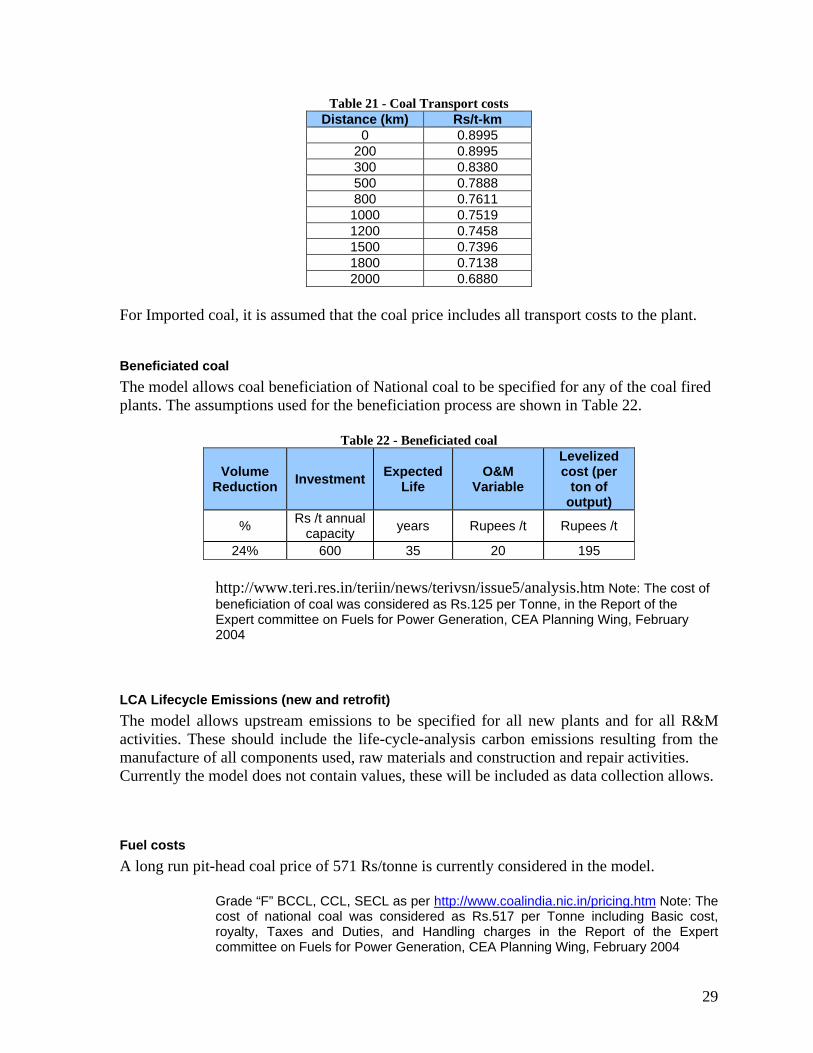
29

Table 21 - Coal Transport costs Distance (km) Rs/t-km

0 0.8995 200 0.8995 300 0.8380 500 0.7888 800 0.7611

1000 0.7519 1200 0.7458 1500 0.7396 1800 0.7138 2000 0.6880

For Imported coal, it is assumed that the coal price includes all transport costs to the plant.

Beneficiated coal

The model allows coal beneficiation of National coal to be specified for any of the coal fired plants. The assumptions used for the beneficiation process are shown in Table 22.

Table 22 - Beneficiated coal

Volume Reduction

Investment Expected

Life O&M

Variable

Levelized cost (per

ton of output)

% Rs /t annual

capacity years Rupees /t Rupees /t

24% 600 35 20 195

http://www.teri.res.in/teriin/news/terivsn/issue5/analysis.htm Note: The cost of beneficiation of coal was considered as Rs.125 per Tonne, in the Report of the Expert committee on Fuels for Power Generation, CEA Planning Wing, February 2004

LCA Lifecycle Emissions (new and retrofit)

The model allows upstream emissions to be specified for all new plants and for all R&M activities. These should include the life-cycle-analysis carbon emissions resulting from the manufacture of all components used, raw materials and construction and repair activities. Currently the model does not contain values, these will be included as data collection allows.

Fuel costs

A long run pit-head coal price of 571 Rs/tonne is currently considered in the model.

Grade “F” BCCL, CCL, SECL as per http://www.coalindia.nic.in/pricing.htm Note: The cost of national coal was considered as Rs.517 per Tonne including Basic cost, royalty, Taxes and Duties, and Handling charges in the Report of the Expert committee on Fuels for Power Generation, CEA Planning Wing, February 2004

30

A pit-head estimated price for Lignite Rajasthan deposits of 800 Rs/ton is considered. Imported coal is currently priced in the model at US$60/tonne.

Based on data from the UMPP risk analysis report by Mott MacDonald (April 2007)

Nuclear is currently priced in the model at Rs 50988 / TJ. Using the calculator at http://www.wise-uranium.org/nfcc.html with an Apr 28, 2008 price of Natural Uranium of US$65/ lb.

The prevailing cost of Naphtha has been taken as Rs. 17,400/tonne (including handling charges of Rs 100 per Tonne at port).

The Report of the Expert committee on Fuels for Power Generation, CEA Planning Wing, February 2004

Fuel calorific values

Indian values taken from CEA documents. Imported coal taken from the UMPP risk analysis report by Mott MacDonald (April 2007)

“All India Electricity Statistics, General Review 2007.” Ministry of Power Government of India, New Delhi CO2 emissions

Results The power sector module is a tool kit that allows an infinite number of scenarios to be investigated and run. To demonstrate its operation, two scenarios have been selected. One (Scenario 1) is based on the goals and commitments laid out in the 11th Plan and associated working group reports. The other (Scenario 2) evaluates slight changes to this plan and how these might affect CO2 emissions, plant investment and operation.

Scenario 1 The initial grid supply condition in the model shows a shortfall at the end of the 10th Plan (2006–07) of 10.9 percent. The forecast assumes that all the system expansion and generation, transmission and distribution improvements contemplated in the 11th plan occur on time and that, as stated by the Working Group Report captive power generation increases from 78,000 GWh in 2006/7 to 131,000 GWh in 2011/2. Since one important goal of the 11th plan is to achieve a spinning reserve of 5 percent on an average annual energy basis by 2011/2, captive power generation is held constant in the model after this date with the rest of electricity being supplied by the grid.

31

Under this scenario, and based on all the Scenario 1 assumptions shown above, the expected combined sum of power supplied to the grid and captive power generated by users increases at an average annual rate of 6.7 percent from 732,000 GWh in 2006/7 to 3,670,000 GWh in 2031/2 as shown in Figure 4.

Figure 4 - Power Generation and CO2 Intensity

0

500,000

1,000,000

1,500,000

2,000,000

2,500,000

3,000,000

3,500,000

4,000,000

2005/6

2007/8

2009/0

2011/2

2013/4

2015/6

2017/8

2019/0

2021/2

2023/4

2025/6

2027/8

2029/0

2031/2

700

750

800

850

900

950

Generation

CO2 Intensity

Generation (GWh) CO2 Intensity (g/kWh)

Installed plated capacity grows from 133,600 MW in 2006/7 to 720,000 MW in 2031/2 at an average annual rate of 7 percent as shown in Figure 5. Over this period, Thermal grows at an annual average rate of 7.0%, Hydro at 5.7% whilst Nuclear maintains an average of 5.0% per year and Renewables 10.8% per year.

Figure 5 - Installed Plated Capacity

0

100,000

200,000

300,000

400,000

500,000

600,000

700,000

800,000

2005

/6

2007

/8

2009

/0

2011

/2

2013

/4

2015

/6

2017

/8

2019

/0

2021

/2

2023

/4

2025

/6

2027

/8

2029

/0

2031

/2

RenewNuclearThermalHydro

Plated Capacity (MW)

To achieve this rate of growth, considerable investment is required. The model builds plants from 2013/4 on, after the completion of those in the 11th Plan. Covering this period, the investment requirement (based on year of start of operation of each plant) increases from Rs 444 [E+09] in 2013/4 to Rs 1900 [E+09] in 2031/2 of which a cumulative 64% is for

32

Thermal followed by 17% for Hydro and 14.3% for Renewables. R&M accounts for less than 3% of the accumulative total. Figure 6 illustrates this requirement whilst Figure 7 shows the required investment on an expenditure flow basis.

Figure 6 - Investment required (Year of Operation)

0

200

400

600

800

1,000

1,200

1,400

1,600

1,800

2,000

2012

/3

2013

/4

2014

/5

2015

/6

2016

/7

2017

/8

2018

/9

2019

/0

2020

/1

2021

/2

2022

/3

2023

/4

2024

/5

2025

/6

2026

/7

2027

/8

2028

/9

2029

/0

2030

/1

2031

/2

R&M (inc T&D)RenewNuclearThermalHydro

Investment Rs [E+09] Year of First Operation

Figure 7 - Investment required (Expenditure Flow Basis) 1. A slower improvement in Transmission and Distribution loss reduction, taking an

additional 5 years to reach 15.05%. 2. LDC: A slow change in the shape of the Load Duration curve, changing from its

historic (2005) shape to that of Thailand (2002) by 2021/2 when GDP per capita PPP will be roughly comparable.

Supply: A slower build-rate for new Hydro and Renewable plants. In scenario 2, the model builds half the new capacity included in scenario 1 of Hydro, Wind and Biomass. New plant

construction between 2013/4 and 2031/2 is limited

to

0

200

400

600

800

1000

1200

1400

1600

1800

2000

2012

/3

2014

/5

2016

/7

2018

/9

2020

/1

2022

/3

2024

/5

2026

/7

2028

/9

2030

/1

R&M (inc T&D)RenewNuclearThermalHydro

Investment Rs [E+09] Expenditure basis

Scenario 2 Scenario 2 contains 3 measures that are compared to Scenario 1, namely:

3. T&D:

33

Hydro: 38,000 MW Wind: 20,800 MW Biomass: 5,205 MW

The impact of these measures is discussed below. Table 25 in appendix A shows the values that important variables assume under scenario 1, scenario 2 and each of the three components of scenario 2 ( T&D, Supply and LDC). Table 23 shows the percentage change of each of these options against scenario 1.

Total generation

In scenario 2, the total generation required into the grid to deliver the same energy supply to end users increases by 3.4% from 48.6 to 50.3 million GWh (48.6 to 50.3 PWh ) over the 26 year period. This is principally because of the slower reduction of Transmission and Distribution (T&D) losses although the change in the shape of the load duration curve and its impact on dispatch also had a minor implication.

Table 23 - Scenario 2 percent change against Scenario 1     Percent change vs Scenario 1 

    +T&D  + Supply  + LDC  Scenario 2 

           

 Total Generation (undiscounted)  GWh  3.1%  0.0%  0.3%  3.4%  Total Generation (Discounted at Financial Analysis rate)  GWh  3.7%  0.0%  0.2%  3.9% 

            

Direct Expenditure           

New Plant Investment  Rs (E+09)  0.0%  ‐7.3%  7.4%  ‐0.3% 

Cost of Renovation or Retrofit  Rs (E+09)  24.2%  ‐2.5%  2.3%  26.4% 

Residual Value of new plant  Rs (E+09)  ‐2.0%  ‐8.7%  7.6%  ‐3.9% 

Residual Value of renovated plant  Rs (E+09)  0.0%  0.0%  0.0%  0.0% 

O&M (Fixed + Variable)  Rs (E+09)  1.9%  0.3%  2.6%  5.0% 

Total fuel cost at Plant  Rs (E+09)  4.4%  3.9%  ‐3.6%  4.6% 

Total Expenditure  Rs (E+09)  3.8%  0.9%  0.5%  5.5% 

            

NPV in year 2005 (Discounted expenditure flow)           

New Plant Investment  Rs (E+09)  2.5%  ‐5.4%  4.9%  2.4% 

Cost of Renovation or Retrofit  Rs (E+09)  ‐16.0%  ‐0.5%  2.4%  ‐13.8% 

Residual Value of new plant  Rs (E+09)  ‐2.0%  ‐8.7%  7.6%  ‐3.9% 

Residual Value of renovated plant  Rs (E+09)  0.0%  0.0%  0.0%  0.0% 

O&M (Fixed + Variable)  Rs (E+09)  1.6%  0.1%  1.2%  3.0% 

Total fuel cost at Plant  Rs (E+09)  6.2%  1.6%  ‐2.3%  5.0% 

Total Expenditure  Rs (E+09)  3.3%  ‐1.3%  1.3%  3.3% 

            

CO2e Emissions (undiscounted)               

Total CO2e emissions from both fuels  Gg  4.1%  4.8%  ‐0.3%  8.7% 

Total CO2e Emissions  Gg  4.1%  4.8%  ‐0.3%  8.7% 

            

CO2e Emissions (Discounted at Financial Analysis rate)  Gg  4.9%  2.3%  ‐0.2%  6.9% 

34

New Plant Investment

In scenario 2, the total investment required for new plants over the complete period remained effectively unchanged (-0.3%) because the reduction of 7.3% in investment due to Supply was offset by an increase of 7.4% due to LDC. It can be seen, though, in the discounted expenditure flow (to 2005) that the timing of the investments differed between the two scenarios with T&D requiring more investment early on (whilst the losses were higher) resulting in a discounted investment 2.3% higher than scenario 1.

Plant Renovation and Retrofit

The total investment in plant renovation and retrofit (R&M) including that required for T&D losses in scenario 2 is higher than the Rs 1.5 [E+12] in scenario 1 by 26.4 % principally because the lag in reducing T&D losses allows the problem is grow and then requires a larger investment at a later date. This time phasing is clearly seen by reviewing the discounted expenditure cash flow where it can be seen that the discounted (to 2005) cost of this line item is lower for scenario 2 than for scenario 1 by 13.3%.

Plant Operations and Maintenance

The total cost of plant operations and maintenance in scenario 2 is 5% higher than the Rs 4.2 [E+12] in scenario 1. This is caused by an increase of 1.9% and 2.6% due to T&D and LDC respectively plus an additional slight increase (0.3%) due to Supply.

Cost of Fuel

The cost of fuel also increases by 4.6% overall from Rs 6 [E+12] in scenario 1. This increase is due to 4.4% caused by T&D, 3.9% caused by Supply offset by an improved utilization of Hydro with the peakier LDC of 3.6%.

Total Expenditure

In direct expenditure over the 26 years in the model, scenario 2 shows an increase of 5.5% when compared to scenario 1. The greatest contributing factor to this difference is T&D. On a discounted expenditure flow basis, scenario 2 requires an increase of 3.4% when compared to scenario 1.

CO2 Emissions

The total CO2 emissions over the 26 year period increased in scenario 2 by 8.8% from the 36.7 thousand million metric tons (36.7 [E+06] Gg) in scenario 1. This increase of 3.2 thousand million metric tons (3.2 [E+06] Gg ) derives in similar proportions from T&D and Supply. Figure 8 shows the difference in carbon intensity of the two scenarios.

35

Figure 8 - Carbon Intensity of Scenarios 1 & 2

700

750

800

850

900

950

2005/6

2007/8

2009/0

2011/2

2013/4

2015/6

2017/8

2019/0

2021/2

2023/4

2025/6

2027/8

2029/0

2031/2

Scenario 2

Scenario 1

CO2 Intensity (g/kWh)

Comparison of Scenario 2 vs Scenario 1

Scenario 2 has a higher total discounted expenditure than scenario 1 by Rs 301 [E+09] or 3.4%. Scenario 2 also has higher CO2 emissions than scenario 1 by 8.8% or 3.2 thousand million metric tons (3.2 [E+06] Gg). Thus the breakeven price of carbon is negative (US$-30.4/t). The impact of each of the components of scenario 2 is as follows:

1. T&D: The 5-year slippage in meeting the Transmission and Distribution loss reduction targets increases the emission of CO2 into the atmosphere by 1,500 million tonnes and increases the overall discounted expenditure flow by Rs 560 [E+09].

2. LDC: The slow change in the shape of the Load Duration curve increases the emission of CO2 into the atmosphere by 92 million tonnes and increases the overall discounted expenditure flow by Rs 213 [E+09].

3. Supply:

The slower build-rate for new Hydro and Renewable plants increases the emission of CO2 into the atmosphere by 1,760 million tonnes but reduces the overall discounted expenditure flow by Rs 213 [E+09]. The breakeven price of carbon of going from this to scenario 1 which is a more costly but cleaner option is US$33.4 /t.

Pair-wise comparison of Technologies Table 24 presents a comparison of distinct technology options against a baseline. In this case the chosen baseline consists of a 500 MW Subcritical coal fired plant using national coal however the model allows any paired comparison to be made.

36

Table 24 - Comparison of Technologies

Plant Type Coal Source 

Capacity MW 

CO2 Emissions  IRR @ US 10c  /kWh 

Breakeven Price of Carbon vs Baseline 

Marginal Abatement Cost vs Baseline Total 

Variable 

Difference vs 

Baseline 

         MW  kg/kWh  kg/kWh  % Rs 

(E+06)/Gg USD /tCO2 

Rs (E+06)/Gg 

USD /tCO2 

Coal  SubCritical  National  500  0.925  Baseline 31.5% 

Baseline 

  SubCritical  National  250  0.933  ‐0.009 29.7% 

‐13.6  ‐340.7  ‐2.5  ‐63.3 

 Low 

Supercritical National  660  0.896  0.029 

30.2% 

1.4  34.5  0.3  6.4 

 High 

Supercritical National  800  0.872  0.053 

29.8% 

1.0  26.2  0.2  4.9 

  Ultracritical  National  1000  0.834  0.091 28.6% 

1.0  26.1  0.2  4.9 

 Ultracritical with CCS 

National  1000  0.160  0.765 19.3% 

1.3  31.6  0.2  5.9 

  SubCritical  Imported  500  0.908  0.016 29.9% 

18.8  469.2  3.5  87.2 

  SubCritical  Imported  250  0.917  0.008 28.8% 

42.4  1060.2  7.9  196.9 

 Low 

Supercritical Imported  660  0.880  0.045 

28.9% 

6.7  167.7  1.2  31.2 

 High 

Supercritical Imported  800  0.857  0.068 

28.4% 

4.6  116.2  0.9  21.6 

  Ultracritical  Imported  1000  0.819  0.106 28.0% 

2.9  72.8  0.5  13.5 

 Ultracritical with CCS 

Imported  1000  0.157  0.768 18.2% 

1.6  40.2  0.3  7.5 

Gas      500  0.489  0.436  2.9%  5.9  148.4  1.1  27.6 

      250  0.489  0.436  2.9%  5.9  148.4  1.1  27.6 

Wind        0.000  0.925 15.1% 

1.5  36.5  0.3  6.8 

Solar        0.000  0.925  2.7%  14.9  372.9  2.8  69.3 

Hydro  Storage      0.000  0.925 18.5% 

0.6  15.9  0.1  1.4 

  RunofRiver      0.000  0.925 21.1% 

0.2  5.8  0.0  0.5 

Nuclear 

      0.000  0.925 22.0% 

0.3  8.2  0.1  1.5 

The calculations in this table consider a coal cost at the plant of Rs 911.4 (US$22.8) per tonne for indigenous coal and Rs 2400 (US$60) per tonne for imported coal including transport. Internal Rates of return (IRR) are calculated based on income from the sale of electricity at an average price of US$0.10/kWh.

37

The breakeven price of carbon shown (in millions of Rupees per gigagram and in Dollars per tonne of carbon dioxide) is the price that should be achieved from the sale of CO2 over the lifetime of the plant to give same net discounted cash flow to that technology when compared with the chosen baseline. In this calculation both income from the sale of carbon and expenditures are discounted using mid-year values of the annual discount rates shown in Table 4. Since the cash flow is discounted to the start of plant operation – which increases the impact of all payments made prior to and during plant construction – and high discount rates minimize the cash-flow impact of long-term emissions savings, the resultant numbers often seem higher than expected. The marginal abatement cost (MAC) shown in the table (in millions of Rupees per gigagram and in Dollars per tonne of carbon dioxide) is the discounted expenditure difference between the selected technology and the baseline divided by the undiscounted CO2 emissions difference between the two. It is apparent that the MAC evaluates the marginal cost of not adding additional tonnes of CO2 to the atmospheric emissions stock where this marginal cost is implicit in having selected a cleaner but more expensive technology than the chosen baseline. In this calculation expenditures are discounted using mid-year values of the annual discount rates shown in Table 4. Here a high discount rate has the tendency to reduce the resultant numbers and pairs with small emissions differences (such as subcritical 500MW and 250 MW plants) can generate large numbers. All of the results shown in Table 24 are sensitive to fuel prices, discount rates, and other factors. Figure 9 shows how the Internal Rate of Return varies with coal prices. The horizontal axis shows the price of coal and the vertical axis the IRR of the plant.

Figure 9 - IRR sensitivity with coal price

15%

17%

19%

21%

23%

25%

27%

29%

31%

33%

35%

20 40 60 80 100

SubCritical 500 MWLow Supercritical 660 MWHigh Supercritical 800 MWUltracritical 1000 MWImported: Low SC 660 MWImported: High SC 800 MWImported: UC 1000 MW

Coal Price at plant (US$/t)

Internal Rate of Return (%)

Figure 10 shows how the Breakeven price of carbon varies with coal prices. The horizontal axis shows the price of indigenous coal and for those plants that use imported coal (lines with

38

markers) a price of US$40 above indigenous coal is used. Thus a breakeven price of zero is found for a low supercritical 660 MW plant using imported coal at US$92/t when compared to a subcritical 500 MW plant using national coal at US$52/t.

Figure 10 - Breakeven price of carbon sensitivity with coal price

‐100

‐50

0

50

100

150

200

250

20 40 60 80 100

Low Supercritical 660 MW

High Supercritical 800 MW

Ultracritical 1000 MW

Imported: Low SC 660 MW

Imported: High SC 800 MW

Imported: UC 1000 MW

Indigenous Coal Price at plant (US$/t)

Breakeven Price of Carbon (US$/t)

[compared with Subcritical 500 MW plant using national coal]

Figure 11 shows the same effect for the Marginal Abatement cost. The horizontal axis shows the price of indigenous coal and for those plants that use imported coal (lines with markers) a price of US$40 above indigenous coal is used. It can be seen that as coal prices rise, it becomes increasingly attractive to use a more efficient plant that consumes less coal and emits less CO2 even though its up-front investment is greater.

Figure 11- Marginal abatement cost sensitivity with coal price

‐20

‐10

0

10

20

30

40

50

20 40 60 80 100

Low Supercritical 660 MWHigh Supercritical 800 MWUltracritical 1000 MWImported: Low SC 660 MWImported: High SC 800 MWImported: UC 1000 MW

Coal Price at plant (US$/t)

Marginal Abatement Cost (US$/t)

[compared with Subcritical 500 MW plant plant using national coal]

39

Appendix 1 Table 25 - Comparison of Scenarios 1 & 2

    Scenario 1  Scenario 1  Scenario 1  Scenario 1  Scenario 2 

       +T&D  + Supply  + LDC    

             

 Total Generation (undiscounted)  GWh  48,630,567  50,145,870  48,630,086  48,788,333  50,307,706 

 Total Generation (Discounted at Financial Analysis rate)  GWh  8,658,545  8,975,522  8,658,485  8,676,767  8,994,390 

              

Direct Sumation             

New Plant Investment  Rs (E+09)  29,009  28,998  26,898  31,161  28,936 

Cost of Renovation or Retrofit  Rs (E+09)  1,490  1,850  1,453  1,525  1,884 

Residual Value of new plant  Rs (E+09)  (17,754)  (17,397)  (16,206)  (19,103)  (17,059) 

Residual Value of renovated plant  Rs (E+09)  (446)  (446)  (446)  (446)  (446) 

O&M (Fixed + Variable)  Rs (E+09)  19,962  20,344  20,017  20,482  20,958 

Total fuel cost at Plant  Rs (E+09)  28,673  29,923  29,793  27,650  30,005 

Total Expenditure  Rs (E+09)  60,934  63,271  61,509  61,268  64,277 

              

NPV in year 2005 (Discounted expenditure flow)             

New Plant Investment  Rs (E+09)  7,099  7,269  6,718  7,449  7,263 

Cost of Renovation or Retrofit  Rs (E+09)  383  324  381  392  332 

Residual Value of new plant  Rs (E+09)  (765)  (750)  (698)  (823)  (735) 

Residual Value of renovated plant  Rs (E+09)  (19)  (19)  (19)  (19)  (19) 

O&M (Fixed + Variable)  Rs (E+09)  4,232  4,299  4,237  4,283  4,361 

Total fuel cost at Plant  Rs (E+09)  6,006  6,374  6,105  5,868  6,307 

Total Expenditure  Rs (E+09)  16,937  17,497  16,724  17,149  17,510 

              

CO2e Emissions (undiscounted)                  

Total CO2e emissions from both fuels  Gg  36,749,719  38,277,816  38,506,800  36,658,037  39,971,119 

Total CO2e Emissions  Gg  36,749,719  38,277,816  38,506,800  36,658,037  39,971,119 

              

CO2e Emissions (Discounted at Financial Analysis rate)  Gg  6,793,603  7,124,038  6,952,935  6,778,736  7,265,591 

Table 26 - Scenario 1 Results India: Low Carbon Growth Study Scenario 1 - Data is for last yearof each PlanPower sector results Data show n for one year (ie: 2005 = fiscal 2005-06)

Units 2005/6 2006/7 2011/2 2016/7 2021/2 2026/7 2031/2

M aximum Plated Capacity

Total Hydro MW 31,970 34,684 57,238 77,164 98,734 118,734 138,734Total Thermal MW 81,828 87,255 141,877 169,541 245,181 343,571 468,312Total Nuclear MW 3,360 3,900 6,420 7,920 9,720 11,280 13,060Total Renew MW 0 7,760 25,070 45,501 70,843 85,893 100,243

Total Maximum Plated Capacity MW 117,158 133,598 230,605 300,127 424,478 559,478 720,349

Generation

Total Hydro GWh 83,579 90,681 150,312 201,859 259,841 310,831 360,227Total Thermal GWh 490,807 511,755 736,498 1,057,383 1,488,404 2,062,877 2,789,405Total Nuclear GWh 26,743 30,976 51,748 62,306 74,931 85,750 98,327Total Renew GWh 0 20,790 66,308 124,520 197,494 242,680 288,595

Total Generation GWh 601,129 654,202 1,004,866 1,446,068 2,020,670 2,702,138 3,536,553

Unit Energy Consumption

Total Hydro MJ/kWh 2.01 2.23 2.63 2.35 1.98 1.71 1.49Total Thermal MJ/kWh 12.62 12.63 11.32 11.53 11.08 10.71 10.59Total Nuclear MJ/kWh 10.70 10.70 10.70 10.99 11.26 11.43 11.57Total Renew MJ/kWh 0.00 0.00 0.00 0.00 0.00 0.00 0.00

Total Unit Energy Consumption MJ/kWh 11.06 10.69 9.24 9.23 8.84 8.73 8.83

Total Energy Consumption

Total Hydro PJ 168 203 396 475 515 530 536Total Thermal PJ 6,192 6,463 8,340 12,186 16,495 22,090 29,538Total Nuclear PJ 286 331 554 684 844 980 1,138Total Renew PJ 0 0 0 0 0 0 0

Total Total Energy Consumption PJ 6,647 6,996 9,289 13,346 17,854 23,600 31,212

Unit Variable CO2e Emissions per GWh

Total Hydro g/kWh 0.00 0.00 0.00 0.00 0.00 0.00 0.00Total Thermal g/kWh 1,115.14 1,120.92 1,021.00 1,037.21 1,001.54 970.64 959.19Total Nuclear g/kWh 0.00 0.00 0.00 0.00 0.00 0.00 0.00Total Renew g/kWh 0.00 0.00 0.00 0.00 0.00 0.00 0.00

Total Unit Variable CO2e Emissions per GWh g/kWh 910.49 876.85 748.33 758.42 737.72 741.01 756.54

Total Variable CO2e Emissions

Total Hydro Gg 0 0 0 0 0 0 0Total Thermal Gg 547,321 573,635 751,967 1,096,726 1,490,693 2,002,314 2,675,559Total Nuclear Gg 0 0 0 0 0 0 0Total Renew Gg 0 0 0 0 0 0 0

Total Total Variable CO2e Emissions Gg 547,321 573,635 751,967 1,096,726 1,490,693 2,002,314 2,675,559

Investment Cash Flow in New

Total Hydro Rupees (E+09) 363.69 228.78 247.64 227.70 213.57 212.00 21.20Total Thermal Rupees (E+09) 148.55 222.32 294.36 561.99 822.31 1,120.63 399.51Total Nuclear Rupees (E+09) 99.78 45.57 18.33 26.00 26.00 26.00 2.60Total Renew Rupees (E+09) 305.03 181.93 207.55 222.06 165.83 150.85 53.74

Total Investment Cash Flow in New Rupees (E+09) 917.04 678.60 767.88 1,037.74 1,227.71 1,509.48 477.04

Investment Cash Flow in Renovation

Total Hydro Rupees (E+09) 0.00 2.34 9.59 15.64 3.22 13.95 2.55Total Thermal Rupees (E+09) 0.00 2.46 4.01 4.32 2.36 3.28 9.04Total Nuclear Rupees (E+09) 0.00 0.00 0.00 0.00 0.00 0.00 0.00Total Renew Rupees (E+09) 0.00 0.00 0.00 0.00 0.00 62.91 49.70

36.24 46.83 33.51 30.60 37.78 0.00 0.00Total Investment Cash Flow in Renovation Rupees (E+09) 36.24 51.62 47.11 50.56 43.37 80.15 61.28

41

Table 27 - Scenario 1 Results

India: Low Carbon Growth Study Scenario 1 - Data is for last yearof each PlanPower sector results Data shown for one year (ie: 2005 = fiscal 2005-06)

Units 2005/6 2006/7 2011/2 2016/7 2021/2 2026/7 2031/2Total Capital Cost (New) Amounts in Year of Operation

Total Hydro Rupees (E+09) 0.00 128.39 558.12 227.70 227.70 212.00 212.00Total Thermal Rupees (E+09) 0.00 35.29 881.54 530.39 783.91 1,107.67 1,331.69Total Nuclear Rupees (E+09) 0.00 0.00 14.30 26.00 26.00 26.00 26.00Total Renew Rupees (E+09) 0.00 344.64 328.65 226.68 243.46 147.44 179.12

Total Investment in New Rupees (E+09) 0.00 508.31 1,782.60 1,010.77 1,281.06 1,493.11 1,748.81

Plant & Equipment (New) Amounts in Year of Operation

Total Hydro Rupees (E+09) 0.00 128.39 558.12 227.70 227.70 212.00 212.00Total Thermal Rupees (E+09) 0.00 35.29 881.54 530.39 783.91 1,107.67 1,331.69Total Nuclear Rupees (E+09) 0.00 0.00 14.30 26.00 26.00 26.00 26.00Total Renew Rupees (E+09) 0.00 344.64 328.65 226.68 243.46 147.44 179.12

Total Plant & Equipment (New) Rupees (E+09) 0.00 508.31 1,782.60 1,010.77 1,281.06 1,493.11 1,748.81

Investment in Renovation Amounts in Year of Operation

Total Hydro Rupees (E+09) 2.10 2.49 10.23 17.76 5.50 19.04 6.36Total Thermal Rupees (E+09) 1.86 1.77 4.33 3.44 2.11 2.86 22.60Total Nuclear Rupees (E+09) 0.00 0.00 0.00 0.00 0.00 0.00 0.00Total Renew Rupees (E+09) 0.00 0.00 0.00 0.00 0.00 103.54 124.25

0.00 0.00 44.11 36.02 35.05 0.00 0.00Total Investment in Renovation Rupees (E+09) 3.97 4.26 58.67 57.22 42.67 125.44 153.20

O&M (Fixed + Variable)

Total Hydro Rupees (E+09) 23.29 24.87 40.48 60.10 81.60 99.60 117.60Total Thermal Rupees (E+09) 347.22 365.72 510.05 574.72 698.97 837.49 1,007.16Total Nuclear Rupees (E+09) 2.45 2.85 4.69 4.61 4.47 4.15 3.99Total Renew Rupees (E+09) 0.00 2.10 9.80 18.83 29.29 33.66 37.80

Total O&M (Fixed + Variable) Rupees (E+09) 372.96 395.54 565.01 658.26 814.33 974.89 1,166.55

Fuel Cost

Total Hydro Rupees (E+09) 0.00 0.00 0.00 0.00 0.00 0.00 0.00Total Thermal Rupees (E+09) 636.25 632.09 550.82 905.13 1,095.11 1,385.54 1,788.34Total Nuclear Rupees (E+09) 14.59 16.90 28.24 34.90 43.04 49.97 58.02Total Renew Rupees (E+09) 0.00 0.00 0.00 0.00 0.00 0.00 0.00

Total Fuel Cost Rupees (E+09) 650.85 648.98 579.06 940.03 1,138.15 1,435.51 1,846.37

42

Table 28 - Scenario 1 Results

India: Low Carbon Growth Study Scenario 1 - Data is for each complete PlanPower sector results Data shown for each five-year plan

Rupees (E+09) 0 Units 2005 - 2032 2007 - 2012 2012 - 2017 2017 - 2022 2022 - 2027 2027 - 2032

Generation

Total Hydro GWh 5,999,018 590,550 897,223 1,184,382 1,452,219 1,700,385

Total Thermal GWh 36,763,821 3,170,542 4,608,625 6,511,030 9,065,389 12,405,672

Total Nuclear GWh 1,822,903 249,901 283,948 352,549 410,579 468,206Total Renew GWh 4,044,825 220,220 490,927 837,642 1,120,884 1,354,363

Total Generation GWh 48,630,567 4,231,213 6,280,724 8,885,603 12,049,071 15,928,625

Total Energy Consumption

Total Hydro PJ 11,904 1,504 2,226 2,509 2,626 2,668Total Thermal PJ 406,986 37,991 53,281 73,088 98,198 131,774Total Nuclear PJ 20,370 2,670 3,085 3,935 4,667 5,395Total Renew PJ 0 0 0 0 0 0

Total Total Energy Consumption PJ 439,260 42,166 58,592 79,532 105,491 139,837

Total Variable CO2e Emissions

Total Hydro Gg 5 0 1 1 1 2Total Thermal Gg 36,749,715 3,410,158 4,788,594 6,596,965 8,893,139 11,939,902Total Nuclear Gg 0 0 0 0 0 0Total Renew Gg 0 0 0 0 0 0

Total Total Variable CO2e Emissions Gg 36,749,719 3,410,159 4,788,594 6,596,966 8,893,140 11,939,904

Investment Cash Flow in New

Total Hydro Rupees (E+09) 5,869 1,420 1,133 1,102 1,060 562Total Thermal Rupees (E+09) 17,766 2,342 1,781 3,540 5,021 4,711Total Nuclear Rupees (E+09) 714 112 127 130 130 69Total Renew Rupees (E+09) 4,660 810 1,001 1,025 706 630

Total Investment Cash Flow in New Rupees (E+09) 29,009 4,684 4,042 5,797 6,918 5,972

Investment Cash Flow in Renovation

Total Hydro Rupees (E+09) 196 27 45 30 44 48Total Thermal Rupees (E+09) 114 19 23 19 19 33Total Nuclear Rupees (E+09) 0 0 0 0 0 0Total Renew Rupees (E+09) 410 0 0 0 125 285

Total Investment Cash Flow in Renovation Rupees (E+09) 1,484 278 226 218 309 366

O&M (Fixed + Variable)

Total Hydro Rupees (E+09) 1,850 165 257 365 462 552Total Thermal Rupees (E+09) 17,422 2,202 2,708 3,233 3,891 4,676Total Nuclear Rupees (E+09) 116 23 23 23 22 20Total Renew Rupees (E+09) 575 32 75 125 159 181

Total O&M (Fixed + Variable) Rupees (E+09) 19,962 2,422 3,063 3,746 4,534 5,430

Fuel Cost

Total Hydro Rupees (E+09) 0 0 0 0 0 0Total Thermal Rupees (E+09) 27,634 2,994 3,990 5,035 6,268 8,078Total Nuclear Rupees (E+09) 1,039 136 157 201 238 275Total Renew Rupees (E+09) 0 0 0 0 0 0

Total Fuel Cost Rupees (E+09) 28,673 3,130 4,148 5,236 6,506 8,353

43

Table 29 - Scenario 2 Results India: Low Carbon Growth Study Scenario 2 - Data is for last yearof each PlanPower sector results Data shown for one year (ie: 2005 = fiscal 2005-06)

Units 2005/6 2006/7 2011/2 2016/7 2021/2 2026/7 2031/2

Maximum Plated Capacity

Total Hydro MW 31,970 34,684 57,238 69,164 80,734 90,734 100,734Total Thermal MW 81,828 87,255 142,377 198,351 294,701 416,951 547,572Total Nuclear MW 3,360 3,900 6,420 7,920 9,720 11,280 13,060Total Renew MW 0 7,760 25,070 42,001 61,388 68,913 76,088

Total Maximum Plated Capacity MW 117,158 133,598 231,105 317,437 446,543 587,878 737,454

Generation

Total Hydro GWh 83,579 90,681 149,483 182,320 211,070 238,476 255,293Total Thermal GWh 490,807 511,755 794,792 1,170,073 1,659,993 2,273,526 2,982,404Total Nuclear GWh 26,743 30,976 51,761 62,345 74,999 85,839 98,430Total Renew GWh 0 20,790 66,314 114,097 169,270 191,907 214,898

Total Generation GWh 601,129 654,202 1,062,350 1,528,835 2,115,331 2,789,748 3,551,026

Unit Energy Consumption

Total Hydro MJ/kWh 2.01 2.23 2.51 2.20 1.95 1.75 1.62Total Thermal MJ/kWh 12.62 12.63 11.46 11.25 10.91 10.78 10.66Total Nuclear MJ/kWh 10.70 10.70 10.70 10.99 11.26 11.43 11.57Total Renew MJ/kWh 0.00 0.00 0.00 0.00 0.00 0.00 0.00

Total Unit Energy Consumption MJ/kWh 11.06 10.69 9.45 9.32 9.15 9.28 9.39

Total Energy Consumption

Total Hydro PJ 168 203 375 401 411 418 412Total Thermal PJ 6,192 6,463 9,112 13,163 18,106 24,498 31,796Total Nuclear PJ 286 331 554 685 845 981 1,139Total Renew PJ 0 0 0 0 0 0 0

Total Total Energy Consumption PJ 6,647 6,996 10,040 14,250 19,362 25,897 33,348

Unit Variable CO2e Emissions per GWh

Total Hydro g/kWh 0.00 0.00 0.00 0.00 0.00 0.00 0.00Total Thermal g/kWh 1,115.14 1,120.92 1,032.59 1,015.14 987.10 975.80 965.78Total Nuclear g/kWh 0.00 0.00 0.00 0.00 0.00 0.00 0.00Total Renew g/kWh 0.00 0.00 0.00 0.00 0.00 0.00 0.00

Total Unit Variable CO2e Emissions per GWh g/kWh 910.49 876.85 772.53 776.92 774.62 795.24 811.13

Total Variable CO2e Emissions

Total Hydro Gg 0 0 0 0 0 1 1Total Thermal Gg 547,321 573,635 820,694 1,187,784 1,638,579 2,218,507 2,880,350Total Nuclear Gg 0 0 0 0 0 0 0Total Renew Gg 0 0 0 0 0 0 0

Total Total Variable CO2e Emissions Gg 547,321 573,635 820,694 1,187,784 1,638,579 2,218,507 2,880,350

Investment Cash Flow in New

Total Hydro Rupees (E+09) 363.69 228.78 178.74 121.70 107.57 106.00 10.60Total Thermal Rupees (E+09) 151.55 227.32 469.93 742.78 1,056.06 1,162.07 441.82Total Nuclear Rupees (E+09) 99.78 45.57 18.33 26.00 26.00 26.00 2.60Total Renew Rupees (E+09) 305.03 181.93 194.62 170.38 100.72 75.42 26.87

Total Investment Cash Flow in New Rupees (E+09) 920.04 683.60 861.62 1,060.86 1,290.35 1,369.50 481.88

Investment Cash Flow in Renovation

Total Hydro Rupees (E+09) 0.00 2.34 9.59 15.64 3.22 13.95 2.55Total Thermal Rupees (E+09) 0.00 2.46 4.01 4.32 2.36 3.28 9.04Total Nuclear Rupees (E+09) 0.00 0.00 0.00 0.00 0.00 0.00 0.00Total Renew Rupees (E+09) 0.00 0.00 0.00 0.00 0.00 62.91 44.57

9.33 16.83 31.46 43.80 58.83 74.48 0.00Total Investment Cash Flow in Renovation Rupees (E+09) 9.33 21.63 45.07 63.76 64.41 154.63 56.15

44

Table 30 - Scenario 2 Results

India: Low Carbon Growth Study Scenario 2 - Data is for last yearof each PlanPower sector results Data shown for one year (ie: 2005 = fiscal 2005-06)

Units 2005/6 2006/7 2011/2 2016/7 2021/2 2026/7 2031/2Total Capital Cost (New) Amounts in Year of Operation

Total Hydro Rupees (E+09) 0.00 128.39 558.12 121.70 121.70 106.00 106.00Total Thermal Rupees (E+09) 0.00 35.29 881.54 657.89 926.82 1,172.50 1,472.72Total Nuclear Rupees (E+09) 0.00 0.00 14.30 26.00 26.00 26.00 26.00Total Renew Rupees (E+09) 0.00 344.64 328.65 172.69 181.08 73.72 89.56

Total Investment in New Rupees (E+09) 0.00 508.31 1,782.60 978.28 1,255.59 1,378.22 1,694.28

Plant & Equipment (New) Amounts in Year of Operation

Total Hydro Rupees (E+09) 0.00 128.39 558.12 121.70 121.70 106.00 106.00Total Thermal Rupees (E+09) 0.00 35.29 881.54 657.89 926.82 1,172.50 1,472.72Total Nuclear Rupees (E+09) 0.00 0.00 14.30 26.00 26.00 26.00 26.00Total Renew Rupees (E+09) 0.00 344.64 328.65 172.69 181.08 73.72 89.56

Total Plant & Equipment (New) Rupees (E+09) 0.00 508.31 1,782.60 978.28 1,255.59 1,378.22 1,694.28

Site Accomodation and Lan Amounts in Year of Operation

Total Hydro Rupees (E+09) 0.00 0.00 0.00 0.00 0.00 0.00 0.00Total Thermal Rupees (E+09) 0.00 0.00 0.00 0.00 0.00 0.00 0.00Total Nuclear Rupees (E+09) 0.00 0.00 0.00 0.00 0.00 0.00 0.00Total Renew Rupees (E+09) 0.00 0.00 0.00 0.00 0.00 0.00 0.00

Total Site Accomodation and Land Rupees (E+09) 0.00 0.00 0.00 0.00 0.00 0.00 0.00

Mgment, Insurance, Spares Amounts in Year of Operation

Total Hydro Rupees (E+09) 0.00 0.00 0.00 0.00 0.00 0.00 0.00Total Thermal Rupees (E+09) 0.00 0.00 0.00 0.00 0.00 0.00 0.00Total Nuclear Rupees (E+09) 0.00 0.00 0.00 0.00 0.00 0.00 0.00Total Renew Rupees (E+09) 0.00 0.00 0.00 0.00 0.00 0.00 0.00

Total Mgment, Insurance, Spares Rupees (E+09) 0.00 0.00 0.00 0.00 0.00 0.00 0.00

Investment in Renovation Amounts in Year of Operation

Total Hydro Rupees (E+09) 2.10 2.49 10.23 17.76 5.50 19.04 6.36Total Thermal Rupees (E+09) 1.86 1.77 4.33 3.44 2.11 2.86 22.60Total Nuclear Rupees (E+09) 0.00 0.00 0.00 0.00 0.00 0.00 0.00Total Renew Rupees (E+09) 0.00 0.00 0.00 0.00 0.00 103.54 111.42

0.00 0.00 28.84 40.47 54.95 71.24 0.00Total Investment in Renovation Rupees (E+09) 3.97 4.26 43.41 61.68 62.56 196.68 140.38

O&M (Fixed + Variable)

Total Hydro Rupees (E+09) 23.29 24.87 40.48 52.90 65.40 74.40 83.40Total Thermal Rupees (E+09) 347.22 365.72 516.84 617.49 768.32 933.08 1,109.05Total Nuclear Rupees (E+09) 2.45 2.85 4.69 4.61 4.47 4.15 3.99Total Renew Rupees (E+09) 0.00 2.10 9.80 17.82 26.54 28.73 30.80

Total O&M (Fixed + Variable) Rupees (E+09) 372.96 395.54 571.80 692.82 864.73 1,040.35 1,227.24

Fuel Cost

Total Hydro Rupees (E+09) 0.00 0.00 0.00 0.00 0.00 0.00 0.00Total Thermal Rupees (E+09) 636.25 632.09 628.92 894.59 1,138.41 1,471.90 1,888.92Total Nuclear Rupees (E+09) 14.59 16.90 28.25 34.92 43.08 50.02 58.08Total Renew Rupees (E+09) 0.00 0.00 0.00 0.00 0.00 0.00 0.00

Total Fuel Cost Rupees (E+09) 650.85 648.98 657.17 929.52 1,181.49 1,521.92 1,947.00

45

Table 31 - Scenario 2 Results

India: Low Carbon Growth Study Scenario 2 - Data is for each complete PlanPower sector results Data shown for each five-year plan

Units 2005 - 2032 2007 - 2012 2012 - 2017 2017 - 2022 2022 - 2027 2027 - 2032

Generation

Total Hydro GWh 4,992,223 590,753 846,438 997,228 1,136,445 1,247,099

Total Thermal GWh 40,105,615 3,356,875 5,044,730 7,254,480 10,074,697 13,372,272

Total Nuclear GWh 1,824,223 249,941 284,065 352,825 410,979 468,694Total Renew GWh 3,385,645 220,231 467,280 734,047 913,180 1,030,116

Total Generation GWh 50,307,706 4,417,800 6,642,513 9,338,580 12,535,301 16,118,182

Total Energy Consumption

Total Hydro PJ 9,967 1,499 1,937 2,019 2,057 2,083Total Thermal PJ 442,519 40,493 57,500 79,810 108,968 143,094Total Nuclear PJ 20,385 2,671 3,086 3,938 4,672 5,401Total Renew PJ 0 0 0 0 0 0

Total Total Energy Consumption PJ 472,871 44,663 62,524 85,767 115,697 150,578

Total Variable CO2e Emissions

Total Hydro Gg 9 1 1 2 3 3Total Thermal Gg 39,971,110 3,625,797 5,180,700 7,217,906 9,863,925 12,961,825Total Nuclear Gg 0 0 0 0 0 0Total Renew Gg 0 0 0 0 0 0

Total Total Variable CO2e Emissions Gg 39,971,119 3,625,798 5,180,701 7,217,908 9,863,928 12,961,828

Investment Cash Flow in New

Total Hydro Rupees (E+09) 3,855 1,266 614 572 530 281Total Thermal Rupees (E+09) 20,887 2,599 2,967 4,460 5,617 4,865Total Nuclear Rupees (E+09) 714 112 127 130 130 69Total Renew Rupees (E+09) 3,480 792 797 735 353 315

Total Investment Cash Flow in New Rupees (E+09) 28,936 4,770 4,505 5,897 6,631 5,530

Investment Cash Flow in Renovation

Total Hydro Rupees (E+09) 196 27 45 30 44 48Total Thermal Rupees (E+09) 114 19 23 19 19 33Total Nuclear Rupees (E+09) 0 0 0 0 0 0Total Renew Rupees (E+09) 372 0 0 0 125 247

Total Investment Cash Flow in Renovation Rupees (E+09) 1,877 184 261 312 529 560

O&M (Fixed + Variable)

Total Hydro Rupees (E+09) 1,508 165 239 302 354 399Total Thermal Rupees (E+09) 18,823 2,224 2,848 3,535 4,337 5,165Total Nuclear Rupees (E+09) 116 23 23 23 22 20Total Renew Rupees (E+09) 511 32 72 115 139 150

Total O&M (Fixed + Variable) Rupees (E+09) 20,958 2,444 3,183 3,975 4,852 5,735

Fuel Cost

Total Hydro Rupees (E+09) 0 0 0 0 0 0Total Thermal Rupees (E+09) 28,966 3,352 4,075 5,127 6,614 8,529Total Nuclear Rupees (E+09) 1,039 136 157 201 238 275Total Renew Rupees (E+09) 0 0 0 0 0 0

Total Fuel Cost Rupees (E+09) 30,005 3,489 4,233 5,327 6,852 8,805