Grey-Level Co-occurrence features for salt texture

classificationIgor Orlov

Master’s thesis presentation

University of Oslo, Department of Informatics

Supervisor: Anne H Schistad Solberg

Content

• Introduction• Problem statement and motivation

• Background• Theoretical review of methods used in thesis

• Implementation• Input data set, finding optimal GLCM parameters

• Evaluation• Finding the best classifier, testing on training and test images

• Summary

Motivation

• Salt structures are closely related to carbohydrates discovery

• Segmentation of salt textures on seismic images is needed to build a correct velocity model

• Time-consuming process, needs automation

Problem statement

Need to segment salt textures on seismic images using grey-level co-occurrence matrices (GLCMs)

Two main goals:

• Provide an algorithm and visualization tool for finding the optimal GLCM parameters, such as offset, direction, window size

• Check whether distance matrix between centers of two classes can be used as a GLCM feature, if yes – estimate performance

Seismic data acquisition

• Initial velocity model is based on mapping of textures to known classes

• Then updated iteratively

• In areas of salt it is hard to build a velocity model, mapping is done manually or semi-aided on each step

Cuts of marine seismic images

Inline slice (vertical cut) Timeslice (horizontal cut)

Data is stored in a 3D cube, can be cut in 2 directions:

Salt texture mapping done manually

Textures in seismic images - inline

• Sub-horizontal reflectors (yellow)

• Up-dipping and down-dipping reflectors (orange)

• Salt structures (blue)

Textures in seismic images - timeslice

• Sub-horizontal reflectors (yellow)

• Steep-dipping reflectors (orange)

• Salt structures (blue)

Not considered in this thesis

Background for research methods

• Grey-level co-occurrence matrices – GLCM

• GLCM features

• Distance metrics

• Gaussian classifier

Grey-level co-occurrence matrix

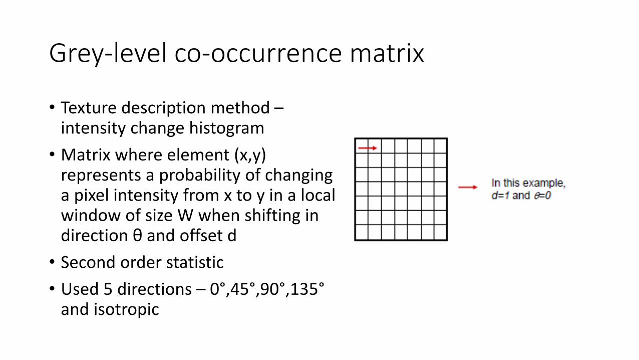
• Texture description method –intensity change histogram

• Matrix where element (x,y) represents a probability of changing a pixel intensity from x to y in a local window of size W when shifting in direction θ and offset d

• Second order statistic

• Used 5 directions – 0°,45°,90°,135°and isotropic

GLCM features

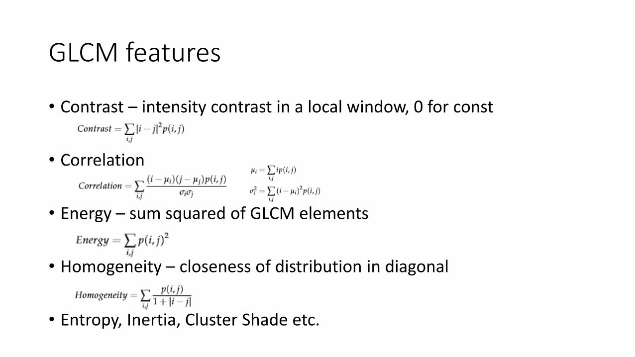
• Contrast – intensity contrast in a local window, 0 for const

• Correlation

• Energy – sum squared of GLCM elements

• Homogeneity – closeness of distribution in diagonal

• Entropy, Inertia, Cluster Shade etc.

Distance metrics

• Used to find a distance between class centers

• Euclidean distance

• Mahalanobis – takes into account in-class distribution (Σ – average covariance matrix), scale invariant

Multivariate Gaussian classifier

• Based on Bayes’ rule

• Assumes Gaussian distribution

• Very simple, trains fast, good enough

• The likelihood that vector xbelongs to class wj

Part 2. Implementation and evaluation

• Input dataset from North Sea

• Finding optimal GLCM parameters, algorithm and visualization

• Mahalanobis distance matrix

• Training Gaussian classifier

• Estimating classification results on training and test images

Input image and mask

Original imageMask. Class 1 – sedimentary rocks (sub-

horizontal), class 2 – salt

Masked and normalized

Image pre-processing

• Input image 1401x1501, [-346;399]

• Cut histogram tails, normalize and shift to [0;255]

• No histogram equalization

Finding the optimal parameters - algorithm

• Choose direction, offset, window size

• For each pixel of class 1, class 2 calculate the GLCM matrix

• Matrix 16x16 can be presented as a feature vector 1x256

• Calculate the average GLCMs for two classes – class centers

• Build a distance matrix where each element is a pixel-wise Mahalanobisdistance between corresponding elements of class center matrices

• Do the same for other direction, offset and window size, compare norm

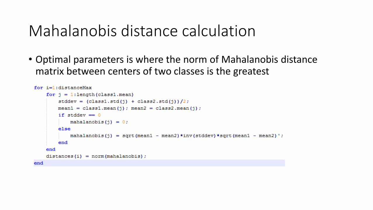
Mahalanobis distance calculation

• Optimal parameters is where the norm of Mahalanobis distance matrix between centers of two classes is the greatest

GLCM parameters

• 16 grey levels, fixed. Thus, all GLCMs had size 16x16

• Window size 31x31, 51x51

• 5 directions

• Which direction is expected to be best?

• Offset 1..15 for 31x31, 1..20 for 51x51

Visualization of distance matrices for 51x51

Horizontal Vertical• Displaying

Mahalanobis distance between average GLCMs for two classes – salt and sedimentary rocks

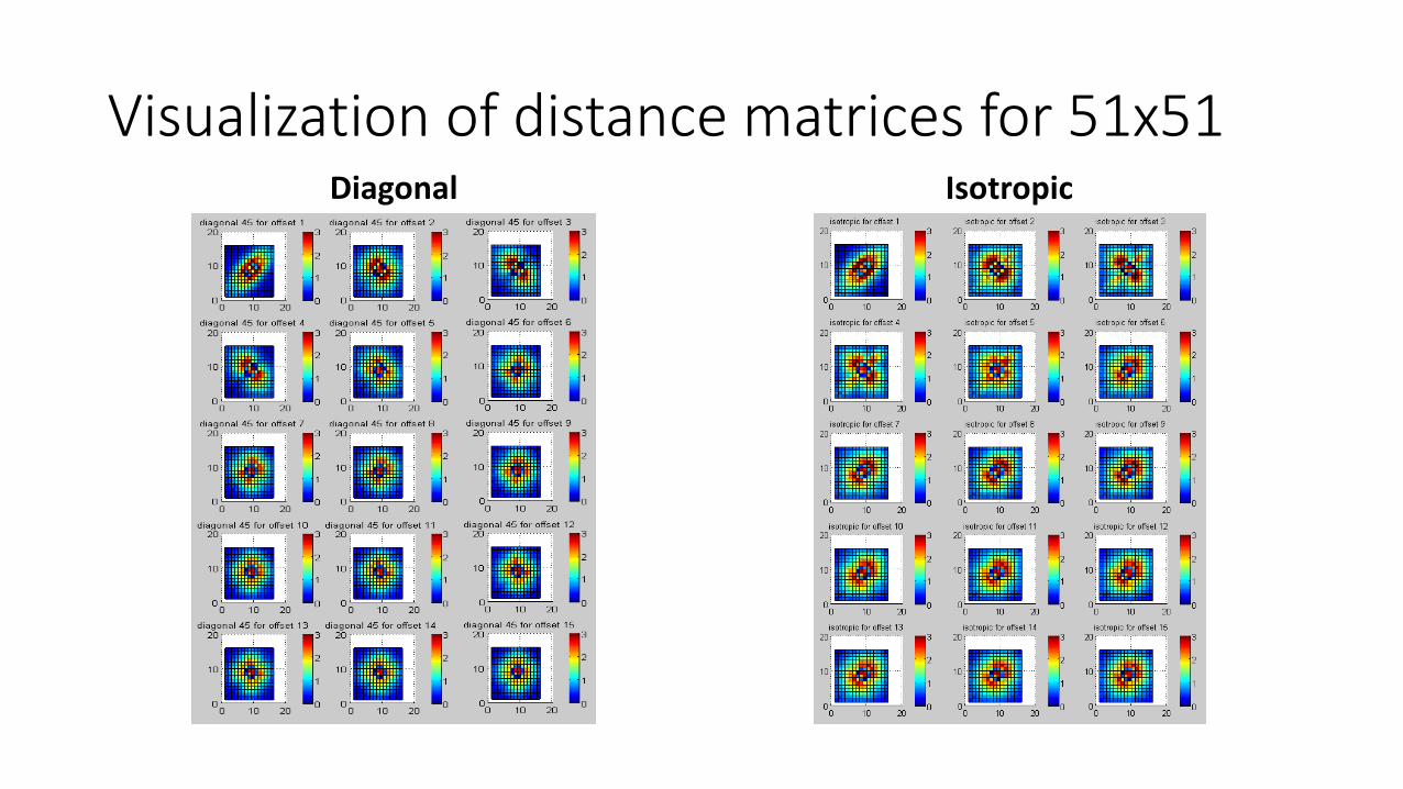
Visualization of distance matrices for 51x51Diagonal Isotropic

Norm of distance matrix, 31x31

Norm of distance matrix, 51x51

Distance matrix for optimal parameters• Suppress values around the center, enhance values in the middle

and on 3-pixel distance around the center

Own GLCM feature

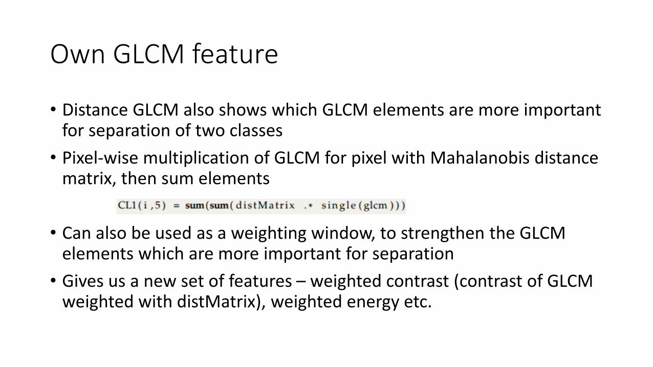
• Distance GLCM also shows which GLCM elements are more important for separation of two classes

• Pixel-wise multiplication of GLCM for pixel with Mahalanobis distance matrix, then sum elements

• Can also be used as a weighting window, to strengthen the GLCM elements which are more important for separation

• Gives us a new set of features – weighted contrast (contrast of GLCM weighted with distMatrix), weighted energy etc.

Feature list

• For each pixel of class 1 and class 2 we have calculated the following ten features:• Variance

• GLCM contrast + weighted

• GLCM energy + weighted

• GLCM correlation + weighted

• GLCM homogeneity + weighted

• Own GLCM feature – sum of weighted GLCM elements

Gaussian classification

• Trained classifier on one-, two-, three-feature subsets – taken manually in a random way

• Some where correlated, overtraining

• One feature is not enough

• Tested on original image (can estimate absolute performance) and 2 test images – only visual estimation

Single feature - Contrast

Single feature – distance GLCM (own)

Single feature – Energy (Weighted)

Classification results for single feature

• For training image, class mapping was provided

• TN – true negative (correctly classified rocks), FP – false positive (rocks classified as salt), TP – true positive (correctly classified salt).

Contrast and Correlation

• Good TN and TP rate is not a guarantee of good results

• TN – 94,17%, TP – 91,8%

Energy and Variance

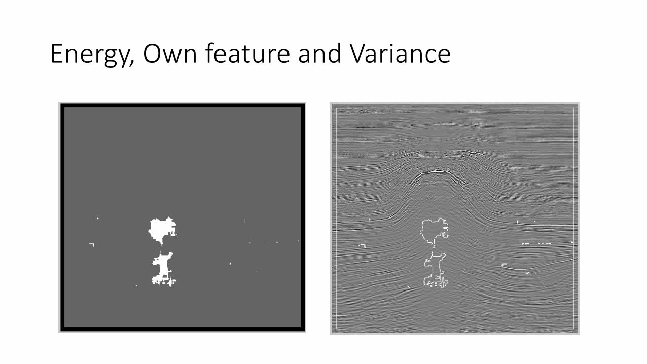
Energy, Own feature and Variance

Contrast, Energy and Own

Contrast, Own and Weighted Energy

Classification results for multiple features

Test images from same dataset

inlinekorr700 inlinekorr780

Classification on test image inlinekorr700

Classification on test image inlinekorr780

Summary - Achieved results

• Found the optimal GLCM parameters for separation of 2 classes:

• Isotropic, offset 2, window 51x51

• Invented and tested own GLCM feature:

• Mahalanobis distance between average GLCMs for two classes

• Trained and tested a set of Gaussian classifiers to find the best feature combination for salt texture extraction

• Visually best is Contrast, Own GLCM and Weighted Energy

Summary – Disadvantages and drawbacks

• Only dataset from North Sea was investigated

• Maximum dimension of Gaussian classifiers was 3

• Only variance, standard Matlab GLCM features (4) and own GLCM feature were tested

• Feature selection done manually

• Only visual testing for test images

Summary - Possible improvements

• 3D GLCM – spatial relationship

• Combination with other texture analysis methods – Fourier transform, greater order statistics etc.

• Own feature – Mahalanobis distance - is based on pixel class mapping. Needs generalization (formula)

The end

Thanks for attention, questions…