gretl command reference - cerge-eihome.cerge-ei.cz/hanousek/mth222/gretl-command-reference.pdf ·...
TRANSCRIPT
Gretl Command Reference
Gnu Regression, Econometrics and Time-series Library
Allin CottrellDepartment of Economics
Wake Forest university
Riccardo “Jack” LucchettiDipartimento di Economia
Università Politecnica delle Marche
March, 2010

Permission is granted to copy, distribute and/or modify this document under the terms ofthe GNU Free Documentation License, Version 1.1 or any later version published by the FreeSoftware Foundation (see http://www.gnu.org/licenses/fdl.html).

Contents
1 Gretl commands 1
1.1 Introduction . . . . . . . . . . . . . . . . . . . . . . . . . . . . . . . . . . . . . . . . . . . . 1
1.2 Commands . . . . . . . . . . . . . . . . . . . . . . . . . . . . . . . . . . . . . . . . . . . . . 1
add . . . . . . . . . . . . . . . . . . . . . . . . . . . . . . . . . . . . . . . . . . . . . . . . . 1
adf . . . . . . . . . . . . . . . . . . . . . . . . . . . . . . . . . . . . . . . . . . . . . . . . . . 2
anova . . . . . . . . . . . . . . . . . . . . . . . . . . . . . . . . . . . . . . . . . . . . . . . . 3
append . . . . . . . . . . . . . . . . . . . . . . . . . . . . . . . . . . . . . . . . . . . . . . . 3
ar . . . . . . . . . . . . . . . . . . . . . . . . . . . . . . . . . . . . . . . . . . . . . . . . . . . 4
ar1 . . . . . . . . . . . . . . . . . . . . . . . . . . . . . . . . . . . . . . . . . . . . . . . . . . 4
arbond . . . . . . . . . . . . . . . . . . . . . . . . . . . . . . . . . . . . . . . . . . . . . . . 5
arch . . . . . . . . . . . . . . . . . . . . . . . . . . . . . . . . . . . . . . . . . . . . . . . . . 5
arima . . . . . . . . . . . . . . . . . . . . . . . . . . . . . . . . . . . . . . . . . . . . . . . . 6
boxplot . . . . . . . . . . . . . . . . . . . . . . . . . . . . . . . . . . . . . . . . . . . . . . . 7
break . . . . . . . . . . . . . . . . . . . . . . . . . . . . . . . . . . . . . . . . . . . . . . . . 8
catch . . . . . . . . . . . . . . . . . . . . . . . . . . . . . . . . . . . . . . . . . . . . . . . . 8
chow . . . . . . . . . . . . . . . . . . . . . . . . . . . . . . . . . . . . . . . . . . . . . . . . . 8
coeffsum . . . . . . . . . . . . . . . . . . . . . . . . . . . . . . . . . . . . . . . . . . . . . . 8
coint . . . . . . . . . . . . . . . . . . . . . . . . . . . . . . . . . . . . . . . . . . . . . . . . . 9
coint2 . . . . . . . . . . . . . . . . . . . . . . . . . . . . . . . . . . . . . . . . . . . . . . . . 9
corr . . . . . . . . . . . . . . . . . . . . . . . . . . . . . . . . . . . . . . . . . . . . . . . . . 10
corrgm . . . . . . . . . . . . . . . . . . . . . . . . . . . . . . . . . . . . . . . . . . . . . . . 10
criteria . . . . . . . . . . . . . . . . . . . . . . . . . . . . . . . . . . . . . . . . . . . . . . . 11
cusum . . . . . . . . . . . . . . . . . . . . . . . . . . . . . . . . . . . . . . . . . . . . . . . . 11
data . . . . . . . . . . . . . . . . . . . . . . . . . . . . . . . . . . . . . . . . . . . . . . . . . 11
dataset . . . . . . . . . . . . . . . . . . . . . . . . . . . . . . . . . . . . . . . . . . . . . . . 12
debug . . . . . . . . . . . . . . . . . . . . . . . . . . . . . . . . . . . . . . . . . . . . . . . . 13
delete . . . . . . . . . . . . . . . . . . . . . . . . . . . . . . . . . . . . . . . . . . . . . . . . 13
diff . . . . . . . . . . . . . . . . . . . . . . . . . . . . . . . . . . . . . . . . . . . . . . . . . . 13
difftest . . . . . . . . . . . . . . . . . . . . . . . . . . . . . . . . . . . . . . . . . . . . . . . 14
discrete . . . . . . . . . . . . . . . . . . . . . . . . . . . . . . . . . . . . . . . . . . . . . . . 14
dummify . . . . . . . . . . . . . . . . . . . . . . . . . . . . . . . . . . . . . . . . . . . . . . 14
duration . . . . . . . . . . . . . . . . . . . . . . . . . . . . . . . . . . . . . . . . . . . . . . 15
elif . . . . . . . . . . . . . . . . . . . . . . . . . . . . . . . . . . . . . . . . . . . . . . . . . . 15
else . . . . . . . . . . . . . . . . . . . . . . . . . . . . . . . . . . . . . . . . . . . . . . . . . 15
end . . . . . . . . . . . . . . . . . . . . . . . . . . . . . . . . . . . . . . . . . . . . . . . . . . 15
endif . . . . . . . . . . . . . . . . . . . . . . . . . . . . . . . . . . . . . . . . . . . . . . . . . 15
i
Contents ii
endloop . . . . . . . . . . . . . . . . . . . . . . . . . . . . . . . . . . . . . . . . . . . . . . . 15
eqnprint . . . . . . . . . . . . . . . . . . . . . . . . . . . . . . . . . . . . . . . . . . . . . . 16
equation . . . . . . . . . . . . . . . . . . . . . . . . . . . . . . . . . . . . . . . . . . . . . . 16
estimate . . . . . . . . . . . . . . . . . . . . . . . . . . . . . . . . . . . . . . . . . . . . . . 16
fcast . . . . . . . . . . . . . . . . . . . . . . . . . . . . . . . . . . . . . . . . . . . . . . . . . 17
foreign . . . . . . . . . . . . . . . . . . . . . . . . . . . . . . . . . . . . . . . . . . . . . . . 18
freq . . . . . . . . . . . . . . . . . . . . . . . . . . . . . . . . . . . . . . . . . . . . . . . . . 18
function . . . . . . . . . . . . . . . . . . . . . . . . . . . . . . . . . . . . . . . . . . . . . . . 19
garch . . . . . . . . . . . . . . . . . . . . . . . . . . . . . . . . . . . . . . . . . . . . . . . . 19
genr . . . . . . . . . . . . . . . . . . . . . . . . . . . . . . . . . . . . . . . . . . . . . . . . . 20
gmm . . . . . . . . . . . . . . . . . . . . . . . . . . . . . . . . . . . . . . . . . . . . . . . . . 22
gnuplot . . . . . . . . . . . . . . . . . . . . . . . . . . . . . . . . . . . . . . . . . . . . . . . 22
graphpg . . . . . . . . . . . . . . . . . . . . . . . . . . . . . . . . . . . . . . . . . . . . . . . 23
hausman . . . . . . . . . . . . . . . . . . . . . . . . . . . . . . . . . . . . . . . . . . . . . . 24
heckit . . . . . . . . . . . . . . . . . . . . . . . . . . . . . . . . . . . . . . . . . . . . . . . . 24
help . . . . . . . . . . . . . . . . . . . . . . . . . . . . . . . . . . . . . . . . . . . . . . . . . 24
hsk . . . . . . . . . . . . . . . . . . . . . . . . . . . . . . . . . . . . . . . . . . . . . . . . . . 25
hurst . . . . . . . . . . . . . . . . . . . . . . . . . . . . . . . . . . . . . . . . . . . . . . . . 25
if . . . . . . . . . . . . . . . . . . . . . . . . . . . . . . . . . . . . . . . . . . . . . . . . . . . 25
include . . . . . . . . . . . . . . . . . . . . . . . . . . . . . . . . . . . . . . . . . . . . . . . 26
info . . . . . . . . . . . . . . . . . . . . . . . . . . . . . . . . . . . . . . . . . . . . . . . . . 26
intreg . . . . . . . . . . . . . . . . . . . . . . . . . . . . . . . . . . . . . . . . . . . . . . . . 26
kalman . . . . . . . . . . . . . . . . . . . . . . . . . . . . . . . . . . . . . . . . . . . . . . . 27
kpss . . . . . . . . . . . . . . . . . . . . . . . . . . . . . . . . . . . . . . . . . . . . . . . . . 27
labels . . . . . . . . . . . . . . . . . . . . . . . . . . . . . . . . . . . . . . . . . . . . . . . . 27
lad . . . . . . . . . . . . . . . . . . . . . . . . . . . . . . . . . . . . . . . . . . . . . . . . . . 27
lags . . . . . . . . . . . . . . . . . . . . . . . . . . . . . . . . . . . . . . . . . . . . . . . . . 28
ldiff . . . . . . . . . . . . . . . . . . . . . . . . . . . . . . . . . . . . . . . . . . . . . . . . . 28
leverage . . . . . . . . . . . . . . . . . . . . . . . . . . . . . . . . . . . . . . . . . . . . . . . 28
logistic . . . . . . . . . . . . . . . . . . . . . . . . . . . . . . . . . . . . . . . . . . . . . . . 29
logit . . . . . . . . . . . . . . . . . . . . . . . . . . . . . . . . . . . . . . . . . . . . . . . . . 29
logs . . . . . . . . . . . . . . . . . . . . . . . . . . . . . . . . . . . . . . . . . . . . . . . . . 30
loop . . . . . . . . . . . . . . . . . . . . . . . . . . . . . . . . . . . . . . . . . . . . . . . . . 30
mahal . . . . . . . . . . . . . . . . . . . . . . . . . . . . . . . . . . . . . . . . . . . . . . . . 31
meantest . . . . . . . . . . . . . . . . . . . . . . . . . . . . . . . . . . . . . . . . . . . . . . 31
mle . . . . . . . . . . . . . . . . . . . . . . . . . . . . . . . . . . . . . . . . . . . . . . . . . . 31
modeltab . . . . . . . . . . . . . . . . . . . . . . . . . . . . . . . . . . . . . . . . . . . . . . 32
modprint . . . . . . . . . . . . . . . . . . . . . . . . . . . . . . . . . . . . . . . . . . . . . . 32
modtest . . . . . . . . . . . . . . . . . . . . . . . . . . . . . . . . . . . . . . . . . . . . . . . 33
mpols . . . . . . . . . . . . . . . . . . . . . . . . . . . . . . . . . . . . . . . . . . . . . . . . 34
negbin . . . . . . . . . . . . . . . . . . . . . . . . . . . . . . . . . . . . . . . . . . . . . . . . 34

Contents iii
nls . . . . . . . . . . . . . . . . . . . . . . . . . . . . . . . . . . . . . . . . . . . . . . . . . . 34
normtest . . . . . . . . . . . . . . . . . . . . . . . . . . . . . . . . . . . . . . . . . . . . . . 35
nulldata . . . . . . . . . . . . . . . . . . . . . . . . . . . . . . . . . . . . . . . . . . . . . . . 36
ols . . . . . . . . . . . . . . . . . . . . . . . . . . . . . . . . . . . . . . . . . . . . . . . . . . 36
omit . . . . . . . . . . . . . . . . . . . . . . . . . . . . . . . . . . . . . . . . . . . . . . . . . 37
open . . . . . . . . . . . . . . . . . . . . . . . . . . . . . . . . . . . . . . . . . . . . . . . . . 38
orthdev . . . . . . . . . . . . . . . . . . . . . . . . . . . . . . . . . . . . . . . . . . . . . . . 39
outfile . . . . . . . . . . . . . . . . . . . . . . . . . . . . . . . . . . . . . . . . . . . . . . . . 39
panel . . . . . . . . . . . . . . . . . . . . . . . . . . . . . . . . . . . . . . . . . . . . . . . . 39
pca . . . . . . . . . . . . . . . . . . . . . . . . . . . . . . . . . . . . . . . . . . . . . . . . . . 40
pergm . . . . . . . . . . . . . . . . . . . . . . . . . . . . . . . . . . . . . . . . . . . . . . . . 40
poisson . . . . . . . . . . . . . . . . . . . . . . . . . . . . . . . . . . . . . . . . . . . . . . . 41
print . . . . . . . . . . . . . . . . . . . . . . . . . . . . . . . . . . . . . . . . . . . . . . . . . 41
printf . . . . . . . . . . . . . . . . . . . . . . . . . . . . . . . . . . . . . . . . . . . . . . . . 42
probit . . . . . . . . . . . . . . . . . . . . . . . . . . . . . . . . . . . . . . . . . . . . . . . . 42
pvalue . . . . . . . . . . . . . . . . . . . . . . . . . . . . . . . . . . . . . . . . . . . . . . . . 43
qlrtest . . . . . . . . . . . . . . . . . . . . . . . . . . . . . . . . . . . . . . . . . . . . . . . . 43
qqplot . . . . . . . . . . . . . . . . . . . . . . . . . . . . . . . . . . . . . . . . . . . . . . . . 44
quantreg . . . . . . . . . . . . . . . . . . . . . . . . . . . . . . . . . . . . . . . . . . . . . . 44
quit . . . . . . . . . . . . . . . . . . . . . . . . . . . . . . . . . . . . . . . . . . . . . . . . . 45
rename . . . . . . . . . . . . . . . . . . . . . . . . . . . . . . . . . . . . . . . . . . . . . . . 45
reset . . . . . . . . . . . . . . . . . . . . . . . . . . . . . . . . . . . . . . . . . . . . . . . . . 45
restrict . . . . . . . . . . . . . . . . . . . . . . . . . . . . . . . . . . . . . . . . . . . . . . . 45
rmplot . . . . . . . . . . . . . . . . . . . . . . . . . . . . . . . . . . . . . . . . . . . . . . . . 47
run . . . . . . . . . . . . . . . . . . . . . . . . . . . . . . . . . . . . . . . . . . . . . . . . . . 47
runs . . . . . . . . . . . . . . . . . . . . . . . . . . . . . . . . . . . . . . . . . . . . . . . . . 47
scatters . . . . . . . . . . . . . . . . . . . . . . . . . . . . . . . . . . . . . . . . . . . . . . . 48
sdiff . . . . . . . . . . . . . . . . . . . . . . . . . . . . . . . . . . . . . . . . . . . . . . . . . 48
set . . . . . . . . . . . . . . . . . . . . . . . . . . . . . . . . . . . . . . . . . . . . . . . . . . 48
setinfo . . . . . . . . . . . . . . . . . . . . . . . . . . . . . . . . . . . . . . . . . . . . . . . 52
setobs . . . . . . . . . . . . . . . . . . . . . . . . . . . . . . . . . . . . . . . . . . . . . . . . 53
setmiss . . . . . . . . . . . . . . . . . . . . . . . . . . . . . . . . . . . . . . . . . . . . . . . 53
shell . . . . . . . . . . . . . . . . . . . . . . . . . . . . . . . . . . . . . . . . . . . . . . . . . 54
smpl . . . . . . . . . . . . . . . . . . . . . . . . . . . . . . . . . . . . . . . . . . . . . . . . . 54
spearman . . . . . . . . . . . . . . . . . . . . . . . . . . . . . . . . . . . . . . . . . . . . . . 55
sprintf . . . . . . . . . . . . . . . . . . . . . . . . . . . . . . . . . . . . . . . . . . . . . . . . 55
square . . . . . . . . . . . . . . . . . . . . . . . . . . . . . . . . . . . . . . . . . . . . . . . . 56
sscanf . . . . . . . . . . . . . . . . . . . . . . . . . . . . . . . . . . . . . . . . . . . . . . . . 56
store . . . . . . . . . . . . . . . . . . . . . . . . . . . . . . . . . . . . . . . . . . . . . . . . . 57
summary . . . . . . . . . . . . . . . . . . . . . . . . . . . . . . . . . . . . . . . . . . . . . . 57
system . . . . . . . . . . . . . . . . . . . . . . . . . . . . . . . . . . . . . . . . . . . . . . . 58

Contents iv
tabprint . . . . . . . . . . . . . . . . . . . . . . . . . . . . . . . . . . . . . . . . . . . . . . . 59
textplot . . . . . . . . . . . . . . . . . . . . . . . . . . . . . . . . . . . . . . . . . . . . . . . 59
tobit . . . . . . . . . . . . . . . . . . . . . . . . . . . . . . . . . . . . . . . . . . . . . . . . . 60
tsls . . . . . . . . . . . . . . . . . . . . . . . . . . . . . . . . . . . . . . . . . . . . . . . . . . 60
var . . . . . . . . . . . . . . . . . . . . . . . . . . . . . . . . . . . . . . . . . . . . . . . . . . 61
varlist . . . . . . . . . . . . . . . . . . . . . . . . . . . . . . . . . . . . . . . . . . . . . . . . 62
vartest . . . . . . . . . . . . . . . . . . . . . . . . . . . . . . . . . . . . . . . . . . . . . . . . 62
vecm . . . . . . . . . . . . . . . . . . . . . . . . . . . . . . . . . . . . . . . . . . . . . . . . . 62
vif . . . . . . . . . . . . . . . . . . . . . . . . . . . . . . . . . . . . . . . . . . . . . . . . . . 63
wls . . . . . . . . . . . . . . . . . . . . . . . . . . . . . . . . . . . . . . . . . . . . . . . . . . 63
xcorrgm . . . . . . . . . . . . . . . . . . . . . . . . . . . . . . . . . . . . . . . . . . . . . . . 63
xtab . . . . . . . . . . . . . . . . . . . . . . . . . . . . . . . . . . . . . . . . . . . . . . . . . 64
1.3 Commands by topic . . . . . . . . . . . . . . . . . . . . . . . . . . . . . . . . . . . . . . . 64
Estimation . . . . . . . . . . . . . . . . . . . . . . . . . . . . . . . . . . . . . . . . . . . . . 64
Tests . . . . . . . . . . . . . . . . . . . . . . . . . . . . . . . . . . . . . . . . . . . . . . . . 65
Transformations . . . . . . . . . . . . . . . . . . . . . . . . . . . . . . . . . . . . . . . . . 65
Statistics . . . . . . . . . . . . . . . . . . . . . . . . . . . . . . . . . . . . . . . . . . . . . . 65
Dataset . . . . . . . . . . . . . . . . . . . . . . . . . . . . . . . . . . . . . . . . . . . . . . . 65
Graphs . . . . . . . . . . . . . . . . . . . . . . . . . . . . . . . . . . . . . . . . . . . . . . . 65
Printing . . . . . . . . . . . . . . . . . . . . . . . . . . . . . . . . . . . . . . . . . . . . . . . 65
Prediction . . . . . . . . . . . . . . . . . . . . . . . . . . . . . . . . . . . . . . . . . . . . . 66
Programming . . . . . . . . . . . . . . . . . . . . . . . . . . . . . . . . . . . . . . . . . . . 66
Utilities . . . . . . . . . . . . . . . . . . . . . . . . . . . . . . . . . . . . . . . . . . . . . . . 66
2 Gretl functions 67
2.1 Introduction . . . . . . . . . . . . . . . . . . . . . . . . . . . . . . . . . . . . . . . . . . . . 67
2.2 Accessors . . . . . . . . . . . . . . . . . . . . . . . . . . . . . . . . . . . . . . . . . . . . . . 67
$ahat . . . . . . . . . . . . . . . . . . . . . . . . . . . . . . . . . . . . . . . . . . . . . . . . 67
$aic . . . . . . . . . . . . . . . . . . . . . . . . . . . . . . . . . . . . . . . . . . . . . . . . . 67
$bic . . . . . . . . . . . . . . . . . . . . . . . . . . . . . . . . . . . . . . . . . . . . . . . . . 67
$chisq . . . . . . . . . . . . . . . . . . . . . . . . . . . . . . . . . . . . . . . . . . . . . . . . 67
$coeff . . . . . . . . . . . . . . . . . . . . . . . . . . . . . . . . . . . . . . . . . . . . . . . . 67
$compan . . . . . . . . . . . . . . . . . . . . . . . . . . . . . . . . . . . . . . . . . . . . . . 68
$datatype . . . . . . . . . . . . . . . . . . . . . . . . . . . . . . . . . . . . . . . . . . . . . . 68
$df . . . . . . . . . . . . . . . . . . . . . . . . . . . . . . . . . . . . . . . . . . . . . . . . . . 68
$dwpval . . . . . . . . . . . . . . . . . . . . . . . . . . . . . . . . . . . . . . . . . . . . . . . 68
$ec . . . . . . . . . . . . . . . . . . . . . . . . . . . . . . . . . . . . . . . . . . . . . . . . . . 68
$error . . . . . . . . . . . . . . . . . . . . . . . . . . . . . . . . . . . . . . . . . . . . . . . . 68
$ess . . . . . . . . . . . . . . . . . . . . . . . . . . . . . . . . . . . . . . . . . . . . . . . . . 68
$Fstat . . . . . . . . . . . . . . . . . . . . . . . . . . . . . . . . . . . . . . . . . . . . . . . . 68
$gmmcrit . . . . . . . . . . . . . . . . . . . . . . . . . . . . . . . . . . . . . . . . . . . . . . 68
$h . . . . . . . . . . . . . . . . . . . . . . . . . . . . . . . . . . . . . . . . . . . . . . . . . . 69

Contents v
$hausman . . . . . . . . . . . . . . . . . . . . . . . . . . . . . . . . . . . . . . . . . . . . . 69
$hqc . . . . . . . . . . . . . . . . . . . . . . . . . . . . . . . . . . . . . . . . . . . . . . . . . 69
$jalpha . . . . . . . . . . . . . . . . . . . . . . . . . . . . . . . . . . . . . . . . . . . . . . . 69
$jbeta . . . . . . . . . . . . . . . . . . . . . . . . . . . . . . . . . . . . . . . . . . . . . . . . 69
$jvbeta . . . . . . . . . . . . . . . . . . . . . . . . . . . . . . . . . . . . . . . . . . . . . . . 69
$lnl . . . . . . . . . . . . . . . . . . . . . . . . . . . . . . . . . . . . . . . . . . . . . . . . . 70
$ncoeff . . . . . . . . . . . . . . . . . . . . . . . . . . . . . . . . . . . . . . . . . . . . . . . 70
$nobs . . . . . . . . . . . . . . . . . . . . . . . . . . . . . . . . . . . . . . . . . . . . . . . . 70
$nvars . . . . . . . . . . . . . . . . . . . . . . . . . . . . . . . . . . . . . . . . . . . . . . . . 70
$pd . . . . . . . . . . . . . . . . . . . . . . . . . . . . . . . . . . . . . . . . . . . . . . . . . 70
$pvalue . . . . . . . . . . . . . . . . . . . . . . . . . . . . . . . . . . . . . . . . . . . . . . . 70
$rho . . . . . . . . . . . . . . . . . . . . . . . . . . . . . . . . . . . . . . . . . . . . . . . . . 70
$rsq . . . . . . . . . . . . . . . . . . . . . . . . . . . . . . . . . . . . . . . . . . . . . . . . . 71
$sample . . . . . . . . . . . . . . . . . . . . . . . . . . . . . . . . . . . . . . . . . . . . . . . 71
$sargan . . . . . . . . . . . . . . . . . . . . . . . . . . . . . . . . . . . . . . . . . . . . . . . 71
$sigma . . . . . . . . . . . . . . . . . . . . . . . . . . . . . . . . . . . . . . . . . . . . . . . 71
$stderr . . . . . . . . . . . . . . . . . . . . . . . . . . . . . . . . . . . . . . . . . . . . . . . 71
$stopwatch . . . . . . . . . . . . . . . . . . . . . . . . . . . . . . . . . . . . . . . . . . . . . 71
$sysA . . . . . . . . . . . . . . . . . . . . . . . . . . . . . . . . . . . . . . . . . . . . . . . . 72
$sysB . . . . . . . . . . . . . . . . . . . . . . . . . . . . . . . . . . . . . . . . . . . . . . . . 72
$sysGamma . . . . . . . . . . . . . . . . . . . . . . . . . . . . . . . . . . . . . . . . . . . . 72
$T . . . . . . . . . . . . . . . . . . . . . . . . . . . . . . . . . . . . . . . . . . . . . . . . . . 72
$t1 . . . . . . . . . . . . . . . . . . . . . . . . . . . . . . . . . . . . . . . . . . . . . . . . . . 72
$t2 . . . . . . . . . . . . . . . . . . . . . . . . . . . . . . . . . . . . . . . . . . . . . . . . . . 72
$test . . . . . . . . . . . . . . . . . . . . . . . . . . . . . . . . . . . . . . . . . . . . . . . . . 72
$trsq . . . . . . . . . . . . . . . . . . . . . . . . . . . . . . . . . . . . . . . . . . . . . . . . . 72
$uhat . . . . . . . . . . . . . . . . . . . . . . . . . . . . . . . . . . . . . . . . . . . . . . . . 72
$unit . . . . . . . . . . . . . . . . . . . . . . . . . . . . . . . . . . . . . . . . . . . . . . . . . 73
$vcv . . . . . . . . . . . . . . . . . . . . . . . . . . . . . . . . . . . . . . . . . . . . . . . . . 73
$version . . . . . . . . . . . . . . . . . . . . . . . . . . . . . . . . . . . . . . . . . . . . . . 73
$windows . . . . . . . . . . . . . . . . . . . . . . . . . . . . . . . . . . . . . . . . . . . . . 73
$xlist . . . . . . . . . . . . . . . . . . . . . . . . . . . . . . . . . . . . . . . . . . . . . . . . 73
$xtxinv . . . . . . . . . . . . . . . . . . . . . . . . . . . . . . . . . . . . . . . . . . . . . . . 73
$yhat . . . . . . . . . . . . . . . . . . . . . . . . . . . . . . . . . . . . . . . . . . . . . . . . 73
2.3 Functions proper . . . . . . . . . . . . . . . . . . . . . . . . . . . . . . . . . . . . . . . . . 73
abs . . . . . . . . . . . . . . . . . . . . . . . . . . . . . . . . . . . . . . . . . . . . . . . . . . 73
acos . . . . . . . . . . . . . . . . . . . . . . . . . . . . . . . . . . . . . . . . . . . . . . . . . 74
acosh . . . . . . . . . . . . . . . . . . . . . . . . . . . . . . . . . . . . . . . . . . . . . . . . 74
asin . . . . . . . . . . . . . . . . . . . . . . . . . . . . . . . . . . . . . . . . . . . . . . . . . 74
asinh . . . . . . . . . . . . . . . . . . . . . . . . . . . . . . . . . . . . . . . . . . . . . . . . 74
atan . . . . . . . . . . . . . . . . . . . . . . . . . . . . . . . . . . . . . . . . . . . . . . . . . 74

Contents vi
atanh . . . . . . . . . . . . . . . . . . . . . . . . . . . . . . . . . . . . . . . . . . . . . . . . 74
bessel . . . . . . . . . . . . . . . . . . . . . . . . . . . . . . . . . . . . . . . . . . . . . . . . 74
BFGSmax . . . . . . . . . . . . . . . . . . . . . . . . . . . . . . . . . . . . . . . . . . . . . . 75
bkfilt . . . . . . . . . . . . . . . . . . . . . . . . . . . . . . . . . . . . . . . . . . . . . . . . . 75
boxcox . . . . . . . . . . . . . . . . . . . . . . . . . . . . . . . . . . . . . . . . . . . . . . . 75
cdemean . . . . . . . . . . . . . . . . . . . . . . . . . . . . . . . . . . . . . . . . . . . . . . 75
cdf . . . . . . . . . . . . . . . . . . . . . . . . . . . . . . . . . . . . . . . . . . . . . . . . . . 76
cdiv . . . . . . . . . . . . . . . . . . . . . . . . . . . . . . . . . . . . . . . . . . . . . . . . . 76
ceil . . . . . . . . . . . . . . . . . . . . . . . . . . . . . . . . . . . . . . . . . . . . . . . . . . 76
cholesky . . . . . . . . . . . . . . . . . . . . . . . . . . . . . . . . . . . . . . . . . . . . . . 77
cmult . . . . . . . . . . . . . . . . . . . . . . . . . . . . . . . . . . . . . . . . . . . . . . . . 77
cnorm . . . . . . . . . . . . . . . . . . . . . . . . . . . . . . . . . . . . . . . . . . . . . . . . 77
colnames . . . . . . . . . . . . . . . . . . . . . . . . . . . . . . . . . . . . . . . . . . . . . . 77
cols . . . . . . . . . . . . . . . . . . . . . . . . . . . . . . . . . . . . . . . . . . . . . . . . . 77
corr . . . . . . . . . . . . . . . . . . . . . . . . . . . . . . . . . . . . . . . . . . . . . . . . . 77
corrgm . . . . . . . . . . . . . . . . . . . . . . . . . . . . . . . . . . . . . . . . . . . . . . . 77
cos . . . . . . . . . . . . . . . . . . . . . . . . . . . . . . . . . . . . . . . . . . . . . . . . . . 78
cosh . . . . . . . . . . . . . . . . . . . . . . . . . . . . . . . . . . . . . . . . . . . . . . . . . 78
cov . . . . . . . . . . . . . . . . . . . . . . . . . . . . . . . . . . . . . . . . . . . . . . . . . . 78
critical . . . . . . . . . . . . . . . . . . . . . . . . . . . . . . . . . . . . . . . . . . . . . . . . 78
cum . . . . . . . . . . . . . . . . . . . . . . . . . . . . . . . . . . . . . . . . . . . . . . . . . 79
deseas . . . . . . . . . . . . . . . . . . . . . . . . . . . . . . . . . . . . . . . . . . . . . . . . 79
det . . . . . . . . . . . . . . . . . . . . . . . . . . . . . . . . . . . . . . . . . . . . . . . . . . 79
diag . . . . . . . . . . . . . . . . . . . . . . . . . . . . . . . . . . . . . . . . . . . . . . . . . 79
diff . . . . . . . . . . . . . . . . . . . . . . . . . . . . . . . . . . . . . . . . . . . . . . . . . . 79
digamma . . . . . . . . . . . . . . . . . . . . . . . . . . . . . . . . . . . . . . . . . . . . . . 79
dnorm . . . . . . . . . . . . . . . . . . . . . . . . . . . . . . . . . . . . . . . . . . . . . . . . 80
dsort . . . . . . . . . . . . . . . . . . . . . . . . . . . . . . . . . . . . . . . . . . . . . . . . . 80
dummify . . . . . . . . . . . . . . . . . . . . . . . . . . . . . . . . . . . . . . . . . . . . . . 80
eigengen . . . . . . . . . . . . . . . . . . . . . . . . . . . . . . . . . . . . . . . . . . . . . . 80
eigensym . . . . . . . . . . . . . . . . . . . . . . . . . . . . . . . . . . . . . . . . . . . . . . 81
exp . . . . . . . . . . . . . . . . . . . . . . . . . . . . . . . . . . . . . . . . . . . . . . . . . . 81
fcstats . . . . . . . . . . . . . . . . . . . . . . . . . . . . . . . . . . . . . . . . . . . . . . . . 81
fdjac . . . . . . . . . . . . . . . . . . . . . . . . . . . . . . . . . . . . . . . . . . . . . . . . . 82
fft . . . . . . . . . . . . . . . . . . . . . . . . . . . . . . . . . . . . . . . . . . . . . . . . . . 82
ffti . . . . . . . . . . . . . . . . . . . . . . . . . . . . . . . . . . . . . . . . . . . . . . . . . . 82
filter . . . . . . . . . . . . . . . . . . . . . . . . . . . . . . . . . . . . . . . . . . . . . . . . . 82
firstobs . . . . . . . . . . . . . . . . . . . . . . . . . . . . . . . . . . . . . . . . . . . . . . . 83
floor . . . . . . . . . . . . . . . . . . . . . . . . . . . . . . . . . . . . . . . . . . . . . . . . . 83
fracdiff . . . . . . . . . . . . . . . . . . . . . . . . . . . . . . . . . . . . . . . . . . . . . . . 83
gammafun . . . . . . . . . . . . . . . . . . . . . . . . . . . . . . . . . . . . . . . . . . . . . 83

Contents vii
getenv . . . . . . . . . . . . . . . . . . . . . . . . . . . . . . . . . . . . . . . . . . . . . . . . 84
gini . . . . . . . . . . . . . . . . . . . . . . . . . . . . . . . . . . . . . . . . . . . . . . . . . . 84
ginv . . . . . . . . . . . . . . . . . . . . . . . . . . . . . . . . . . . . . . . . . . . . . . . . . 84
hpfilt . . . . . . . . . . . . . . . . . . . . . . . . . . . . . . . . . . . . . . . . . . . . . . . . 84
I . . . . . . . . . . . . . . . . . . . . . . . . . . . . . . . . . . . . . . . . . . . . . . . . . . . 84
imaxc . . . . . . . . . . . . . . . . . . . . . . . . . . . . . . . . . . . . . . . . . . . . . . . . 84
imaxr . . . . . . . . . . . . . . . . . . . . . . . . . . . . . . . . . . . . . . . . . . . . . . . . 85
imhof . . . . . . . . . . . . . . . . . . . . . . . . . . . . . . . . . . . . . . . . . . . . . . . . 85
iminc . . . . . . . . . . . . . . . . . . . . . . . . . . . . . . . . . . . . . . . . . . . . . . . . 85
iminr . . . . . . . . . . . . . . . . . . . . . . . . . . . . . . . . . . . . . . . . . . . . . . . . 85
infnorm . . . . . . . . . . . . . . . . . . . . . . . . . . . . . . . . . . . . . . . . . . . . . . . 85
int . . . . . . . . . . . . . . . . . . . . . . . . . . . . . . . . . . . . . . . . . . . . . . . . . . 85
inv . . . . . . . . . . . . . . . . . . . . . . . . . . . . . . . . . . . . . . . . . . . . . . . . . . 86
invcdf . . . . . . . . . . . . . . . . . . . . . . . . . . . . . . . . . . . . . . . . . . . . . . . . 86
invpd . . . . . . . . . . . . . . . . . . . . . . . . . . . . . . . . . . . . . . . . . . . . . . . . 86
irr . . . . . . . . . . . . . . . . . . . . . . . . . . . . . . . . . . . . . . . . . . . . . . . . . . 86
islist . . . . . . . . . . . . . . . . . . . . . . . . . . . . . . . . . . . . . . . . . . . . . . . . . 86
isnull . . . . . . . . . . . . . . . . . . . . . . . . . . . . . . . . . . . . . . . . . . . . . . . . 87
kdensity . . . . . . . . . . . . . . . . . . . . . . . . . . . . . . . . . . . . . . . . . . . . . . 87
kfilter . . . . . . . . . . . . . . . . . . . . . . . . . . . . . . . . . . . . . . . . . . . . . . . . 87
ksimul . . . . . . . . . . . . . . . . . . . . . . . . . . . . . . . . . . . . . . . . . . . . . . . . 87
ksmooth . . . . . . . . . . . . . . . . . . . . . . . . . . . . . . . . . . . . . . . . . . . . . . 88
isseries . . . . . . . . . . . . . . . . . . . . . . . . . . . . . . . . . . . . . . . . . . . . . . . 88
isstring . . . . . . . . . . . . . . . . . . . . . . . . . . . . . . . . . . . . . . . . . . . . . . . 88
lags . . . . . . . . . . . . . . . . . . . . . . . . . . . . . . . . . . . . . . . . . . . . . . . . . 88
lastobs . . . . . . . . . . . . . . . . . . . . . . . . . . . . . . . . . . . . . . . . . . . . . . . 88
ldet . . . . . . . . . . . . . . . . . . . . . . . . . . . . . . . . . . . . . . . . . . . . . . . . . 88
ldiff . . . . . . . . . . . . . . . . . . . . . . . . . . . . . . . . . . . . . . . . . . . . . . . . . 89
lincomb . . . . . . . . . . . . . . . . . . . . . . . . . . . . . . . . . . . . . . . . . . . . . . . 89
ljungbox . . . . . . . . . . . . . . . . . . . . . . . . . . . . . . . . . . . . . . . . . . . . . . 89
lngamma . . . . . . . . . . . . . . . . . . . . . . . . . . . . . . . . . . . . . . . . . . . . . . 89
log . . . . . . . . . . . . . . . . . . . . . . . . . . . . . . . . . . . . . . . . . . . . . . . . . . 89
log10 . . . . . . . . . . . . . . . . . . . . . . . . . . . . . . . . . . . . . . . . . . . . . . . . 89
log2 . . . . . . . . . . . . . . . . . . . . . . . . . . . . . . . . . . . . . . . . . . . . . . . . . 90
logistic . . . . . . . . . . . . . . . . . . . . . . . . . . . . . . . . . . . . . . . . . . . . . . . 90
lower . . . . . . . . . . . . . . . . . . . . . . . . . . . . . . . . . . . . . . . . . . . . . . . . 90
lrvar . . . . . . . . . . . . . . . . . . . . . . . . . . . . . . . . . . . . . . . . . . . . . . . . . 90
makemask . . . . . . . . . . . . . . . . . . . . . . . . . . . . . . . . . . . . . . . . . . . . . 90
max . . . . . . . . . . . . . . . . . . . . . . . . . . . . . . . . . . . . . . . . . . . . . . . . . 90
maxc . . . . . . . . . . . . . . . . . . . . . . . . . . . . . . . . . . . . . . . . . . . . . . . . . 91
maxr . . . . . . . . . . . . . . . . . . . . . . . . . . . . . . . . . . . . . . . . . . . . . . . . . 91

Contents viii
mcorr . . . . . . . . . . . . . . . . . . . . . . . . . . . . . . . . . . . . . . . . . . . . . . . . 91
mcov . . . . . . . . . . . . . . . . . . . . . . . . . . . . . . . . . . . . . . . . . . . . . . . . 91
mcovg . . . . . . . . . . . . . . . . . . . . . . . . . . . . . . . . . . . . . . . . . . . . . . . . 91
mean . . . . . . . . . . . . . . . . . . . . . . . . . . . . . . . . . . . . . . . . . . . . . . . . 91
meanc . . . . . . . . . . . . . . . . . . . . . . . . . . . . . . . . . . . . . . . . . . . . . . . . 92
meanr . . . . . . . . . . . . . . . . . . . . . . . . . . . . . . . . . . . . . . . . . . . . . . . . 92
median . . . . . . . . . . . . . . . . . . . . . . . . . . . . . . . . . . . . . . . . . . . . . . . 92
mexp . . . . . . . . . . . . . . . . . . . . . . . . . . . . . . . . . . . . . . . . . . . . . . . . 92
min . . . . . . . . . . . . . . . . . . . . . . . . . . . . . . . . . . . . . . . . . . . . . . . . . 92
minc . . . . . . . . . . . . . . . . . . . . . . . . . . . . . . . . . . . . . . . . . . . . . . . . . 92
minr . . . . . . . . . . . . . . . . . . . . . . . . . . . . . . . . . . . . . . . . . . . . . . . . . 92
missing . . . . . . . . . . . . . . . . . . . . . . . . . . . . . . . . . . . . . . . . . . . . . . . 93
misszero . . . . . . . . . . . . . . . . . . . . . . . . . . . . . . . . . . . . . . . . . . . . . . 93
mlag . . . . . . . . . . . . . . . . . . . . . . . . . . . . . . . . . . . . . . . . . . . . . . . . . 93
mnormal . . . . . . . . . . . . . . . . . . . . . . . . . . . . . . . . . . . . . . . . . . . . . . 93
mols . . . . . . . . . . . . . . . . . . . . . . . . . . . . . . . . . . . . . . . . . . . . . . . . . 93
movavg . . . . . . . . . . . . . . . . . . . . . . . . . . . . . . . . . . . . . . . . . . . . . . . 94
mpols . . . . . . . . . . . . . . . . . . . . . . . . . . . . . . . . . . . . . . . . . . . . . . . . 94
mread . . . . . . . . . . . . . . . . . . . . . . . . . . . . . . . . . . . . . . . . . . . . . . . . 94
mreverse . . . . . . . . . . . . . . . . . . . . . . . . . . . . . . . . . . . . . . . . . . . . . . 94
mshape . . . . . . . . . . . . . . . . . . . . . . . . . . . . . . . . . . . . . . . . . . . . . . . 95
msortby . . . . . . . . . . . . . . . . . . . . . . . . . . . . . . . . . . . . . . . . . . . . . . . 95
muniform . . . . . . . . . . . . . . . . . . . . . . . . . . . . . . . . . . . . . . . . . . . . . 95
mwrite . . . . . . . . . . . . . . . . . . . . . . . . . . . . . . . . . . . . . . . . . . . . . . . 95
mxtab . . . . . . . . . . . . . . . . . . . . . . . . . . . . . . . . . . . . . . . . . . . . . . . . 95
nelem . . . . . . . . . . . . . . . . . . . . . . . . . . . . . . . . . . . . . . . . . . . . . . . . 96
nobs . . . . . . . . . . . . . . . . . . . . . . . . . . . . . . . . . . . . . . . . . . . . . . . . . 96
normal . . . . . . . . . . . . . . . . . . . . . . . . . . . . . . . . . . . . . . . . . . . . . . . 96
npv . . . . . . . . . . . . . . . . . . . . . . . . . . . . . . . . . . . . . . . . . . . . . . . . . 96
nullspace . . . . . . . . . . . . . . . . . . . . . . . . . . . . . . . . . . . . . . . . . . . . . . 96
obs . . . . . . . . . . . . . . . . . . . . . . . . . . . . . . . . . . . . . . . . . . . . . . . . . . 97
obslabel . . . . . . . . . . . . . . . . . . . . . . . . . . . . . . . . . . . . . . . . . . . . . . . 97
obsnum . . . . . . . . . . . . . . . . . . . . . . . . . . . . . . . . . . . . . . . . . . . . . . . 97
ok . . . . . . . . . . . . . . . . . . . . . . . . . . . . . . . . . . . . . . . . . . . . . . . . . . 97
onenorm . . . . . . . . . . . . . . . . . . . . . . . . . . . . . . . . . . . . . . . . . . . . . . 97
ones . . . . . . . . . . . . . . . . . . . . . . . . . . . . . . . . . . . . . . . . . . . . . . . . . 98
orthdev . . . . . . . . . . . . . . . . . . . . . . . . . . . . . . . . . . . . . . . . . . . . . . . 98
pdf . . . . . . . . . . . . . . . . . . . . . . . . . . . . . . . . . . . . . . . . . . . . . . . . . . 98
pergm . . . . . . . . . . . . . . . . . . . . . . . . . . . . . . . . . . . . . . . . . . . . . . . . 98
pmax . . . . . . . . . . . . . . . . . . . . . . . . . . . . . . . . . . . . . . . . . . . . . . . . 98
pmean . . . . . . . . . . . . . . . . . . . . . . . . . . . . . . . . . . . . . . . . . . . . . . . . 99

Contents ix
pmin . . . . . . . . . . . . . . . . . . . . . . . . . . . . . . . . . . . . . . . . . . . . . . . . . 99
pnobs . . . . . . . . . . . . . . . . . . . . . . . . . . . . . . . . . . . . . . . . . . . . . . . . 99
polroots . . . . . . . . . . . . . . . . . . . . . . . . . . . . . . . . . . . . . . . . . . . . . . . 99
princomp . . . . . . . . . . . . . . . . . . . . . . . . . . . . . . . . . . . . . . . . . . . . . . 99
psd . . . . . . . . . . . . . . . . . . . . . . . . . . . . . . . . . . . . . . . . . . . . . . . . . . 100
psdroot . . . . . . . . . . . . . . . . . . . . . . . . . . . . . . . . . . . . . . . . . . . . . . . 100
pvalue . . . . . . . . . . . . . . . . . . . . . . . . . . . . . . . . . . . . . . . . . . . . . . . . 100
qform . . . . . . . . . . . . . . . . . . . . . . . . . . . . . . . . . . . . . . . . . . . . . . . . 101
qnorm . . . . . . . . . . . . . . . . . . . . . . . . . . . . . . . . . . . . . . . . . . . . . . . . 101
qrdecomp . . . . . . . . . . . . . . . . . . . . . . . . . . . . . . . . . . . . . . . . . . . . . 101
quantile . . . . . . . . . . . . . . . . . . . . . . . . . . . . . . . . . . . . . . . . . . . . . . . 101
rank . . . . . . . . . . . . . . . . . . . . . . . . . . . . . . . . . . . . . . . . . . . . . . . . . 101
ranking . . . . . . . . . . . . . . . . . . . . . . . . . . . . . . . . . . . . . . . . . . . . . . . 101
randgen . . . . . . . . . . . . . . . . . . . . . . . . . . . . . . . . . . . . . . . . . . . . . . . 102
rcond . . . . . . . . . . . . . . . . . . . . . . . . . . . . . . . . . . . . . . . . . . . . . . . . 102
readfile . . . . . . . . . . . . . . . . . . . . . . . . . . . . . . . . . . . . . . . . . . . . . . . 103
replace . . . . . . . . . . . . . . . . . . . . . . . . . . . . . . . . . . . . . . . . . . . . . . . 103
resample . . . . . . . . . . . . . . . . . . . . . . . . . . . . . . . . . . . . . . . . . . . . . . 103
round . . . . . . . . . . . . . . . . . . . . . . . . . . . . . . . . . . . . . . . . . . . . . . . . 104
rows . . . . . . . . . . . . . . . . . . . . . . . . . . . . . . . . . . . . . . . . . . . . . . . . . 104
sd . . . . . . . . . . . . . . . . . . . . . . . . . . . . . . . . . . . . . . . . . . . . . . . . . . 104
sdc . . . . . . . . . . . . . . . . . . . . . . . . . . . . . . . . . . . . . . . . . . . . . . . . . . 104
sdiff . . . . . . . . . . . . . . . . . . . . . . . . . . . . . . . . . . . . . . . . . . . . . . . . . 104
selifc . . . . . . . . . . . . . . . . . . . . . . . . . . . . . . . . . . . . . . . . . . . . . . . . . 104
selifr . . . . . . . . . . . . . . . . . . . . . . . . . . . . . . . . . . . . . . . . . . . . . . . . . 105
seq . . . . . . . . . . . . . . . . . . . . . . . . . . . . . . . . . . . . . . . . . . . . . . . . . . 105
sin . . . . . . . . . . . . . . . . . . . . . . . . . . . . . . . . . . . . . . . . . . . . . . . . . . 105
sinh . . . . . . . . . . . . . . . . . . . . . . . . . . . . . . . . . . . . . . . . . . . . . . . . . 105
sort . . . . . . . . . . . . . . . . . . . . . . . . . . . . . . . . . . . . . . . . . . . . . . . . . 105
sortby . . . . . . . . . . . . . . . . . . . . . . . . . . . . . . . . . . . . . . . . . . . . . . . . 105
sqrt . . . . . . . . . . . . . . . . . . . . . . . . . . . . . . . . . . . . . . . . . . . . . . . . . 106
sscanf . . . . . . . . . . . . . . . . . . . . . . . . . . . . . . . . . . . . . . . . . . . . . . . . 106
sst . . . . . . . . . . . . . . . . . . . . . . . . . . . . . . . . . . . . . . . . . . . . . . . . . . 106
strlen . . . . . . . . . . . . . . . . . . . . . . . . . . . . . . . . . . . . . . . . . . . . . . . . 106
strncmp . . . . . . . . . . . . . . . . . . . . . . . . . . . . . . . . . . . . . . . . . . . . . . . 106
strstr . . . . . . . . . . . . . . . . . . . . . . . . . . . . . . . . . . . . . . . . . . . . . . . . 106
sum . . . . . . . . . . . . . . . . . . . . . . . . . . . . . . . . . . . . . . . . . . . . . . . . . 107
sumc . . . . . . . . . . . . . . . . . . . . . . . . . . . . . . . . . . . . . . . . . . . . . . . . 107
sumr . . . . . . . . . . . . . . . . . . . . . . . . . . . . . . . . . . . . . . . . . . . . . . . . . 107
svd . . . . . . . . . . . . . . . . . . . . . . . . . . . . . . . . . . . . . . . . . . . . . . . . . . 107
tan . . . . . . . . . . . . . . . . . . . . . . . . . . . . . . . . . . . . . . . . . . . . . . . . . . 107

Contents x
tanh . . . . . . . . . . . . . . . . . . . . . . . . . . . . . . . . . . . . . . . . . . . . . . . . . 108
toepsolv . . . . . . . . . . . . . . . . . . . . . . . . . . . . . . . . . . . . . . . . . . . . . . 108
tolower . . . . . . . . . . . . . . . . . . . . . . . . . . . . . . . . . . . . . . . . . . . . . . . 108
tr . . . . . . . . . . . . . . . . . . . . . . . . . . . . . . . . . . . . . . . . . . . . . . . . . . . 108
transp . . . . . . . . . . . . . . . . . . . . . . . . . . . . . . . . . . . . . . . . . . . . . . . . 108
trimr . . . . . . . . . . . . . . . . . . . . . . . . . . . . . . . . . . . . . . . . . . . . . . . . . 108
uniform . . . . . . . . . . . . . . . . . . . . . . . . . . . . . . . . . . . . . . . . . . . . . . . 109
unvech . . . . . . . . . . . . . . . . . . . . . . . . . . . . . . . . . . . . . . . . . . . . . . . 109
upper . . . . . . . . . . . . . . . . . . . . . . . . . . . . . . . . . . . . . . . . . . . . . . . . 109
urcpval . . . . . . . . . . . . . . . . . . . . . . . . . . . . . . . . . . . . . . . . . . . . . . . 109
values . . . . . . . . . . . . . . . . . . . . . . . . . . . . . . . . . . . . . . . . . . . . . . . . 110
var . . . . . . . . . . . . . . . . . . . . . . . . . . . . . . . . . . . . . . . . . . . . . . . . . . 110
varname . . . . . . . . . . . . . . . . . . . . . . . . . . . . . . . . . . . . . . . . . . . . . . 110
varnum . . . . . . . . . . . . . . . . . . . . . . . . . . . . . . . . . . . . . . . . . . . . . . . 110
vec . . . . . . . . . . . . . . . . . . . . . . . . . . . . . . . . . . . . . . . . . . . . . . . . . . 110
vech . . . . . . . . . . . . . . . . . . . . . . . . . . . . . . . . . . . . . . . . . . . . . . . . . 110
weekday . . . . . . . . . . . . . . . . . . . . . . . . . . . . . . . . . . . . . . . . . . . . . . 111
wmean . . . . . . . . . . . . . . . . . . . . . . . . . . . . . . . . . . . . . . . . . . . . . . . 111
wsd . . . . . . . . . . . . . . . . . . . . . . . . . . . . . . . . . . . . . . . . . . . . . . . . . 111
wvar . . . . . . . . . . . . . . . . . . . . . . . . . . . . . . . . . . . . . . . . . . . . . . . . . 111
xmax . . . . . . . . . . . . . . . . . . . . . . . . . . . . . . . . . . . . . . . . . . . . . . . . 111
xmin . . . . . . . . . . . . . . . . . . . . . . . . . . . . . . . . . . . . . . . . . . . . . . . . . 112
xpx . . . . . . . . . . . . . . . . . . . . . . . . . . . . . . . . . . . . . . . . . . . . . . . . . . 112
zeromiss . . . . . . . . . . . . . . . . . . . . . . . . . . . . . . . . . . . . . . . . . . . . . . 112
zeros . . . . . . . . . . . . . . . . . . . . . . . . . . . . . . . . . . . . . . . . . . . . . . . . 112
3 Comments in scripts 113
4 Options, arguments and path-searching 115
4.1 Invoking gretl . . . . . . . . . . . . . . . . . . . . . . . . . . . . . . . . . . . . . . . . . . . 115
4.2 Preferences dialog . . . . . . . . . . . . . . . . . . . . . . . . . . . . . . . . . . . . . . . . 115
4.3 Invoking gretlcli . . . . . . . . . . . . . . . . . . . . . . . . . . . . . . . . . . . . . . . . . . 116
4.4 Path searching . . . . . . . . . . . . . . . . . . . . . . . . . . . . . . . . . . . . . . . . . . . 116
MS Windows . . . . . . . . . . . . . . . . . . . . . . . . . . . . . . . . . . . . . . . . . . . . 117
5 Reserved Words 118

Chapter 1
Gretl commands
1.1 Introduction
The commands defined below may be executed interactively in the command-line client pro-gram or in the console window of the GUI program. They may also be placed in a “script” orbatch file for non-interactive execution.
The following notational conventions are used below:
• A typewriter font is used for material that you would type directly, and also for internalnames of variables.
• Terms in a slanted font are place-holders: you should substitute some specific replace-ment. For example, you might type income in place of the generic xvar.
• The construction [ arg ] means that the argument arg is optional: you may supply it ornot (but in any case don’t type the brackets).
• The phrase “estimation command” means a command that generates estimates for a givenmodel, for example ols, ar or wls.
In general, each line of a command script should contain one and only one complete gretlcommand. There are, however, two means of continuing a long command from one line ofinput to another. First, if the last non-space character on a line is a backslash, this is taken asan indication that the command is continued on the following line. In addition, if the comma isa valid character in a given command (for instance, as a separator between function arguments,or as punctuation in the commands printf and sscanf) then a trailing comma also indicatescontinuation. To emphasize the point: a backslash may be inserted “arbitrarily” to indicatecontinuation, but a comma works in this capacity only if it is syntactically valid as part of thecommand.
1.2 Commands
add
Argument: varlist
Options: --vcv (print covariance matrix)
--quiet (don’t print estimates for augmented model)
--silent (don’t print anything)
--inst (add as instrument, TSLS only)
--both (add as both regressor and instrument, TSLS only)
Examples: add 5 7 9
add xx yy zz --quiet
Must be invoked after an estimation command. The variables in varlist are added to the pre-vious model and the new model is estimated. A test statistic for the joint significance of theadded variables is printed, along with its p-value. The test statistic is F in the case of OLS es-timation, an asymptotic Wald chi-square value otherwise. A p-value below 0.05 means that thecoefficients are jointly significant at the 5 percent level.
If the --quiet option is given the printed results are confined to the test for the joint signifi-cance of the added variables, otherwise the estimates for the augmented model are also printed.
1

Chapter 1. Gretl commands 2
In the latter case, the --vcv flag causes the covariance matrix for the coefficients to be printedalso. If the --silent option is given, nothing is printed; nonetheless, the results of the test canbe retrieved using the special variables $test and $pvalue.
If the original model was estimated using two-stage least squares, an ambiguity arises: shouldthe new variables be added as regressors, as instruments, or as both? This is resolved asfollows: by default the new variables are added as endogenous regressors, but if the --instflag is given they are added as instruments, or if the --both flag is given they are added asexogenous regressors.
Menu path: Model window, /Tests/Add variables
adf
Arguments: order varlist
Options: --nc (test without a constant)
--c (with constant only)
--ct (with constant and trend)
--ctt (with constant, trend and trend squared)
--seasonals (include seasonal dummy variables)
--gls (de-mean or de-trend using GLS)
--verbose (print regression results)
--quiet (suppress printing of results)
--difference (use first difference of variable)
--test-down (automatic lag order)
Examples: adf 0 y
adf 2 y --nc --c --ct
adf 12 y --c --test-down
See also jgm-1996.inp
Computes a set of Dickey–Fuller tests on each of the the listed variables, the null hypothesisbeing that the variable in question has a unit root. (But if the --difference flag is given, thefirst difference of the variable is taken prior to testing, and the discussion below must be takenas referring to the transformed variable.)
By default, two variants of the test are shown: one based on a regression containing a constantand one using a constant and linear trend. You can control the variants that are presented byspecifying one or more of the option flags.
In all cases the dependent variable is the first difference of the specified variable, y , and thekey independent variable is the first lag of y . The model is constructed so that the coefficienton lagged y equals the root in question minus 1. For example, the model with a constant maybe written as
(1− L)yt = β0 + (α− 1)yt−1 + εtUnder the null hypothesis of a unit root the coefficient on lagged y equals zero; under thealternative that y is stationary this coefficient is negative.
If the lag order, k, is greater than 0, then k lags of the dependent variable are included on theright-hand side of the test regressions, subject to the following qualification. If the --test-downoption is given, k is taken as the maximum lag and the actual lag order used is obtained by test-ing down, using this algorithm:
1. Estimate the Dickey–Fuller regression with k lags of the dependent variable.
2. Is the last lag significant? If so, execute the test with lag order k. Otherwise, let k = k − 1;if k equals 0, execute the test with lag order 0, else go to step 1.
In the context of step 2 above, “significant” means that the t-statistic for the last lag has anasymptotic two-sided p-value, against the normal distribution, of 0.10 or less.

Chapter 1. Gretl commands 3
The --gls option can be used in conjunction with one or other of the flags --c and --ct (themodel with constant, or model with constant and trend). The effect of this option is that the de-meaning or de-trending of the variable to be tested is done using the GLS procedure suggestedby Elliott, Rothenberg and Stock (1996), which gives a test of greater power than the standardDickey–Fuller approach. This option is not compatible with --nc, --ctt or --seasonals.
P-values for the Dickey–Fuller tests are based on MacKinnon (1996). The relevant code is in-cluded by kind permission of the author. In the case of the test with linear trend using GLSthese P-values are not applicable; critical values from Table 1 in Elliott, Rothenberg and Stock(1996) are shown instead.
Menu path: /Variable/Augmented Dickey-Fuller test
anova
Arguments: response treatment [ block ]
Option: --quiet (don’t print results)
Analysis of Variance: response is a series measuring some effect of interest and treatmentmust be a discrete variable that codes for two or more types of treatment (or non-treatment).For two-way ANOVA, the block variable (which should also be discrete) codes for the values ofsome control variable.
Unless the --quiet option is given, this command prints a table showing the sums of squaresand mean squares along with an F -test. The F -test and its P-value can be retrieved using theaccessors $test and $pvalue respectively.
The null hypothesis for the F -test is that the mean response is invariant with respect to thetreatment type, or in words that the treatment has no effect. Strictly speaking, the test is validonly if the variance of the response is the same for all treatment types.
Note that the results shown by this command are in fact a subset of the information given bythe following procedure, which is easily implemented in gretl. Create a set of dummy variablescoding for all but one of the treatment types. For two-way ANOVA, in addition create a set ofdummies coding for all but one of the “blocks”. Then regress response on a constant and thedummies using ols. For a one-way design the ANOVA table is printed via the --anova option tools. In the two-way case the relevant F -test is found by using the omit command. For example(assuming y is the response, xt codes for the treatment, and xb codes for blocks):
# one-waylist dxt = dummify(xt)ols y 0 dxt --anova# two-waylist dxb = dummify(xb)ols y 0 dxt dxb# test joint significance of dxtomit dxt --quiet
Menu path: /Model/Other linear models/ANOVA
append
Argument: datafile
Option: --time-series (see below)
Opens a data file and appends the content to the current dataset, if the new data are compatible.The program will try to detect the format of the data file (native, plain text, CSV, Gnumeric,Excel, etc.).
The appended data may take the form of either additional observations on variables alreadypresent in the dataset, or new variables. in the case of adding variables, compatibility requireseither (a) that the number of observations for the new data equals that for the current data, or

Chapter 1. Gretl commands 4
(b) that the new data carries clear observation information so that gretl can work out how toplace the values.
A special feature is supported for appending to a panel dataset. Let n denote the number ofcross-sectional units in the panel, T denote the number of time periods, and m denote thenumber of observations for the new data. Ifm = n the new data are taken to be time-invariant,and are copied into place for each time period. On the other hand, ifm = T the data are treatedas non-varying across the panel units, and are copied into place for each unit. If the panel is“square”, and m equals both n and T , an ambiguity arises. The default in this case is to treatthe new data as time-invariant, but you can force gretl to treat the new data as time series viathe --time-series option. (This option is ignored in all other cases.)
Menu path: /File/Append data
ar
Arguments: lags ; depvar indepvars
Option: --vcv (print covariance matrix)
Example: ar 1 3 4 ; y 0 x1 x2 x3
Computes parameter estimates using the generalized Cochrane–Orcutt iterative procedure (seeSection 9.5 of Ramanathan, 2002). Iteration is terminated when successive error sums ofsquares do not differ by more than 0.005 percent or after 20 iterations.
lags is a list of lags in the residuals, terminated by a semicolon. In the above example, the errorterm is specified as
ut = ρ1ut−1 + ρ3ut−3 + ρ4ut−4 + et
Menu path: /Model/Time series/Autoregressive estimation
ar1
Arguments: depvar indepvars
Options: --hilu (use Hildreth–Lu procedure)
--pwe (use Prais–Winsten estimator)
--vcv (print covariance matrix)
--no-corc (do not fine-tune results with Cochrane-Orcutt)
Examples: ar1 1 0 2 4 6 7
ar1 y 0 xlist --hilu --no-corc
ar1 y 0 xlist --pwe
Computes feasible GLS estimates for a model in which the error term is assumed to follow afirst-order autoregressive process.
The default method is the Cochrane–Orcutt iterative procedure (see, for example, Section 9.4 ofRamanathan, 2002). Iteration is terminated when successive estimates of the autocorrelationcoefficient do not differ by more than 0.001 or after 20 iterations.
If the --hilu option is given, the Hildreth–Lu search procedure is used. The results are thenfine-tuned using the Cochrane–Orcutt method, unless the --no-corc flag is specified. (Thelatter option is ignored if --hilu is not specified.)
If the --pwe option is given, the Prais–Winsten estimator is used. This involves an an iterationsimilar to Cochrane–Orcutt; the difference is that while Cochrane–Orcutt discards the first ob-servation, Prais–Winsten makes use of it. See, for example, Chapter 13 of Greene’s EconometricAnalysis (2000) for details.
Menu path: /Model/Time series/Cochrane-Orcutt
Menu path: /Model/Time series/Hildreth-Lu
Menu path: /Model/Time series/Prais-Winsten
Chapter 1. Gretl commands 5
arbond
Argument: p [ q ] ; depvar indepvars [ ; instruments ]
Options: --quiet (don’t show estimated model)
--vcv (print covariance matrix)
--two-step (perform 2-step GMM estimation)
--time-dummies (add time dummy variables)
--asymptotic (uncorrected asymptotic standard errors)
Examples: arbond 2 ; y Dx1 Dx2
arbond 2 5 ; y Dx1 Dx2 ; Dx1
arbond 1 ; y Dx1 Dx2 ; Dx1 GMM(x2,2,3)
See also arbond91.inp
Carries out estimation of dynamic panel data models (that is, panel models including one ormore lags of the dependent variable) using the GMM method set out by Arellano and Bond(1991).
The parameter p represents the order of the autoregression for the dependent variable. Theoptional parameter q indicates the maximum lag of the level of the dependent variable to beused as an instrument. If this argument is omitted, or given as 0, all available lags are used.
The dependent variable should be given in levels form; it will be automatically differenced (sincethis estimator uses differencing to cancel out the individual effects). The independent variablesare not automatically differenced; if you want to use differences (which will generally be thecase for ordinary quantitative variables, though perhaps not for, say, time dummy variables)you should create the differences first then specify these as the regressors.
The last (optional) field in the command is for specifying instruments. If no instruments aregiven, it is assumed that all the independent variables are strictly exogenous. If you specify anyinstruments, you should include in the list any strictly exogenous independent variables. Forpredetermined regressors, you can use the GMM function to include a specified range of lags inblock-diagonal fashion. This is illustrated in the third example above. The first argument toGMM is the name of the variable in question, the second is the minimum lag to be used as aninstrument, and the third is the maximum lag. If the third argument is given as 0, all availablelags are used.
By default the results of 1-step estimation are reported (with robust standard errors). You mayselect 2-step estimation as an option. In both cases tests for autocorrelation of orders 1 and 2are provided, as well as the Sargan overidentification test and a Wald test for the joint signif-icance of the regressors. Note that in this differenced model first-order autocorrelation is nota threat to the validity of the model, but second-order autocorrelation violates the maintainedstatistical assumptions.
In the case of 2-step estimation, standard errors are by default computed using the finite-samplecorrection suggested by Windmeijer (2005). The standard asymptotic standard errors associ-ated with the 2-step estimator are generally reckoned to be an unreliable guide to inference, butif for some reason you want to see them you can use the --asymptotic option to turn off theWindmeijer correction.
If the --time-dummies option is given, a set of time dummy variables is added to the specifiedregressors. The number of dummies is one less than the maximum number of periods used inestimation, to avoid perfect collinearity with the constant. The dummies are entered in levels;if you wish to use time dummies in first-differenced form, you will have to define and add thesevariables manually.
Menu path: /Model/Panel
arch
Arguments: order depvar indepvars
Example: arch 4 y 0 x1 x2 x3

Chapter 1. Gretl commands 6
Estimates the given model specification allowing for ARCH (Autoregressive Conditional Hetero-skedasticity). The model is first estimated via OLS, then an auxiliary regression is run, in whichthe squared residual from the first stage is regressed on its own lagged values. The final step isweighted least squares estimation, using as weights the reciprocals of the fitted error variancesfrom the auxiliary regression. (If the predicted variance of any observation in the auxiliaryregression is not positive, then the corresponding squared residual is used instead).
The alpha values displayed below the coefficients are the estimated parameters of the ARCHprocess from the auxiliary regression.
See also garch and modtest (the --arch option).
Menu path: /Model/Time series/ARCH
arima
Arguments: p d q [ ; P D Q ] ; depvar [ indepvars ]
Options: --verbose (print details of iterations)
--vcv (print covariance matrix)
--opg (see below)
--nc (do not include a constant)
--conditional (use conditional maximum likelihood)
--x-12-arima (use X-12-ARIMA for estimation)
--lbfgs (use L-BFGS-B maximizer)
--y-diff-only (ARIMAX special, see below)
--continue (continue on numerical errors)
Examples: arima 1 0 2 ; y
arima 2 0 2 ; y 0 x1 x2 --verbose
arima 0 1 1 ; 0 1 1 ; y --nc
If no indepvars list is given, estimates a univariate ARIMA (Autoregressive, Integrated, MovingAverage) model. The values p, d and q represent the autoregressive (AR) order, the differencingorder, and the moving average (MA) order respectively. These values may be given in numericalform, or as the names of pre-existing scalar variables. A d value of 1, for instance, meansthat the first difference of the dependent variable should be taken before estimating the ARMAparameters.
If you wish to include only specific AR or MA lags in the model (as opposed to all lags up toa given order) you can substitute for p and/or q either (a) the name of a pre-defined matrixcontaining a set of integer values or (b) an expression such as {1 4}; that is, a set of lagsseparated by spaces and enclosed in braces.
The optional integer values P, D and Q represent the seasonal AR, order for seasonal differenc-ing and seasonal MA order respectively. These are applicable only if the data have a frequencygreater than 1 (for example, quarterly or monthly data). These orders must be given in numeri-cal form or as scalar variables.
In the univariate case the default is to include an intercept in the model but this can be sup-pressed with the --nc flag. If indepvars are added, the model becomes ARMAX; in this casethe constant should be included explicitly if you want an intercept (as in the second exampleabove).
An alternative form of syntax is available for this command: if you do not want to apply dif-ferencing (either seasonal or non-seasonal), you may omit the d and D fields altogether, ratherthan explicitly entering 0. In addition, arma is a synonym or alias for arima. Thus for examplethe following command is a valid way to specify an ARMA(2, 1) model:
arma 2 1 ; y
The default is to use the “native” gretl ARMA functionality, with estimation by exact ML usingthe Kalman filter; estimation via conditional ML is available as an option. (If X-12-ARIMA is

Chapter 1. Gretl commands 7
installed you have the option of using it instead of native code.) For details regarding theseoptions, please see the Gretl User’s Guide.
When the native ARMA code is used, estimated standard errors are by default based on a nu-merical approximation to the (negative inverse of) the Hessian. But if the --opg option is giventhey are instead based on the Outer Product of the Gradient. This option is ignored if estimationvia X-12-ARIMA is selected.
The option --lbfgs is specific to estimation using native ARMA code and exact ML: it calls foruse of the “limited memory” L-BFGS-B algorithm in place of the regular BFGS maximizer. Thismay help in some instances where convergence is difficult to achieve.
The option --y-diff-only is specific to estimation of ARIMAX models (models with a non-zeroorder of integration and including exogenous regressors), and applies only when gretl’s nativeexact ML is used. For such models the default behavior is to difference both the dependentvariable and the regressors, but when this option is specified only the dependent variable isdifferenced, the regressors remaining in level form.
In general if a gretl command fails to complete successfully, execution of a script is halted.However, if the --continue option is given for this command, execution continues providedthat that error is “numerical” (e.g. failure to converge, to the specified tolerance). In this casethe internal variable $error is set to a non-zero value; accessing this variable causes it to becleared to zero. See the set command for related ways of controlling gretl’s behavior.
The AIC value given in connection with ARIMA models is calculated according to the definitionused in X-12-ARIMA, namely
AIC = −2` + 2kwhere ` is the log-likelihood and k is the total number of parameters estimated. Note that X-12-ARIMA does not produce information criteria such as AIC when estimation is by conditionalML.
The “frequency” figure printed in connection with AR and MA roots is the λ value that solves
z = rei2πλ
where z is the root in question and r is its modulus.
Menu path: /Model/Time series/ARIMA
Other access: Main window pop-up menu (single selection)
boxplot
Argument: varlist
Options: --notches (show 90 percent interval for median)
--output=filename (send output to specified file)
These plots (after Tukey and Chambers) display the distribution of a variable. The central boxencloses the middle 50 percent of the data, i.e. it is bounded by the first and third quartiles.The “whiskers” extend to the minimum and maximum values. A line is drawn across the box atthe median. A “+” sign indicates the mean.
In the case of notched boxes, the notch shows the limits of an approximate 90 percent confi-dence interval for the median. This is obtained by the bootstrap method.
After each variable specified in the boxplot command, a parenthesized Boolean expression maybe added, to limit the sample for the variable in question. A space must be inserted betweenthe variable name or number and the expression. Suppose you have salary figures for men andwomen, and you have a dummy variable GENDER with value 1 for men and 0 for women. In thatcase you could draw comparative boxplots with the following varlist:
salary (GENDER=1) salary (GENDER=0)
In interactive mode the result is displayed immediately. In batch mode the default behavior isthat a gnuplot command file is written in the user’s working directory, with a name on the pat-tern gpttmpN.plt, starting with N = 01. The actual plots may be generated later using gnuplot

Chapter 1. Gretl commands 8
(under MS Windows, wgnuplot). This behavior can be modified by use of the --output=filenameoption. For details, please see the gnuplot command.
Menu path: /View/Graph specified vars/Boxplots
break
Break out of a loop. This command can be used only within a loop; it causes command executionto break out of the current (innermost) loop. See also loop.
catch
Syntax: catch command
This is not a command in its own right but can be used as a prefix to most regular commands:the effect is to prevent termination of a script if an error occurs in executing the command. Ifan error does occur, this is registered in an internal error code which can be accessed as $error(a zero value indicates success). The value of $error should always be checked immediatelyafter using catch, and appropriate action taken if the command failed.
chow
Variants: chow obs
chow dummyvar --dummy
Options: --dummy (use a pre-existing dummy variable)
--quiet (don’t print estimates for augmented model)
Examples: chow 25
chow 1988:1
chow female --dummy
Must follow an OLS regression. If an observation number or date is given, provides a test forthe null hypothesis of no structural break at the given split point. The procedure is to create adummy variable which equals 1 from the split point specified by obs to the end of the sample,0 otherwise, and also interaction terms between this dummy and the original regressors. If adummy variable is given, tests the null hypothesis of structural homogeneity with respect tothat dummy. Again, interaction terms are added. In either case an augmented regression is runincluding the additional terms.
By default an F statistic is calculated, taking the augmented regression as the unrestrictedmodel and the original as the restricted. But if the original model used a robust estimator forthe covariance matrix, the test statistic is a Wald chi-square value based on a robust estimatorof the covariance matrix for the augmented regression.
Menu path: Model window, /Tests/Chow test
coeffsum
Argument: varlist
Example: coeffsum xt xt_1 xr_2
restrict.inp
Must follow a regression. Calculates the sum of the coefficients on the variables in varlist. Printsthis sum along with its standard error and the p-value for the null hypothesis that the sum iszero.
Note the difference between this and omit, which tests the null hypothesis that the coefficientson a specified subset of independent variables are all equal to zero.
Menu path: Model window, /Tests/Sum of coefficients

Chapter 1. Gretl commands 9
coint
Arguments: order depvar indepvars
Options: --nc (do not include a constant)
--ct (include constant and trend)
--ctt (include constant and quadratic trend)
--skip-df (no DF tests on individual variables)
--test-down (automatic lag order)
Examples: coint 4 y x1 x2
coint 0 y x1 x2 --ct --skip-df
The Engle–Granger cointegration test. The default procedure is: (1) carry out Dickey–Fuller testson the null hypothesis that each of the variables listed has a unit root; (2) estimate the cointe-grating regression; and (3) run a DF test on the residuals from the cointegrating regression. Ifthe --skip-df flag is given, step (1) is omitted.
If the specified lag order is positive all the Dickey–Fuller tests use that order, with this qualifi-cation: if the --test-down option is given, the given value is taken as the maximum and theactual lag order used in each case is obtained by testing down. See the adf command for detailsof this procedure.
By default, the cointegrating regression contains a constant. If you wish to suppress the con-stant, add the --nc flag. If you wish to augment the list of deterministic terms in the cointe-grating regression with a linear or quadratic trend, add the --ct or --ctt flag. These optionflags are mutually exclusive.
P-values for this test are based on MacKinnon (1996). The relevant code is included by kindpermission of the author.
Menu path: /Model/Time series/Cointegration test/Engle-Granger
coint2
Arguments: order ylist [ ; xlist ] [ ; rxlist ]
Options: --nc (no constant)
--rc (restricted constant)
--crt (constant and restricted trend)
--ct (constant and unrestricted trend)
--seasonals (include centered seasonal dummies)
--quiet (print just the tests)
--verbose (print details of auxiliary regressions)
Examples: coint2 2 y x
coint2 4 y x1 x2 --verbose
coint2 3 y x1 x2 --rc
Carries out the Johansen test for cointegration among the variables in ylist for the given lagorder. Critical values are computed via J. Doornik’s gamma approximation (Doornik, 1998). Fordetails of this test see Hamilton, Time Series Analysis (1994), Chapter 20.
The inclusion of deterministic terms in the model is controlled by the option flags. The defaultif no option is specified is to include an “unrestricted constant”, which allows for the presenceof a non-zero intercept in the cointegrating relations as well as a trend in the levels of theendogenous variables. In the literature stemming from the work of Johansen (see for examplehis 1995 book) this is often referred to as “case 3”. The first four options given above, whichare mutually exclusive, produce cases 1, 2, 4 and 5 respectively. The meaning of these casesand the criteria for selecting a case are explained in the Gretl User’s Guide.
The optional lists xlist and rxlist allow you to control for specified exogenous variables: theseenter the system either unrestrictedly (xlist) or restricted to the cointegration space (rxlist).These lists are separated from ylist and from each other by semicolons.

Chapter 1. Gretl commands 10
The --seasonals option, which may be combined with any of the other options, specifiesthe inclusion of a set of centered seasonal dummy variables. This option is available only forquarterly or monthly data.
The following table is offered as a guide to the interpretation of the results shown for the test,for the 3-variable case. H0 denotes the null hypothesis, H1 the alternative hypothesis, and c thenumber of cointegrating relations.
Trace test λ-max test
Rank H0 H1 H0 H1
0 c = 0 c = 3 c = 0 c = 1
1 c = 1 c = 3 c = 1 c = 2
2 c = 2 c = 3 c = 2 c = 3
See also the vecm command.
Menu path: /Model/Time series/Cointegration test/Johansen
corr
Argument: [ varlist ]
Options: --uniform (ensure uniform sample)
--spearman (Spearman’s rho)
--kendall (Kendall’s tau)
--verbose (print rankings)
Examples: corr y x1 x2 x3
corr ylist --uniform
corr x y --spearman
By default, prints the pairwise correlation coefficients (Pearson’s product-moment correlation)for the variables in varlist, or for all variables in the data set if varlist is not given. The standardbehavior is to use all available observations for computing each pairwise coefficient, but ifthe --uniform option is given the sample is limited (if necessary) so that the same set ofobservations is used for all the coefficients. This option has an effect only if there are differingnumbers of missing values for the variables used.
The (mutually exclusive) options --spearman and --kendall produce, respectively, Spear-man’s rank correlation rho and Kendall’s rank correlation tau in place of the default Pearsoncoefficient. When either of these options is given, varlist should contain just two variables.
When a rank correlation is computed, the verbose option can be used to print the original andranked data (otherwise this option is ignored).
Menu path: /View/Correlation matrix
Other access: Main window pop-up menu (multiple selection)
corrgm
Arguments: variable [ maxlag ]
Option: --quiet (don’t draw ACF graph)
Example: corrgm x 12
Prints the values of the autocorrelation function for variable, which may be specified by nameor number. The values are defined as ρ(ut , ut−s) where ut is the tth observation of the variableu and s is the number of lags.
The partial autocorrelations (calculated using the Durbin–Levinson algorithm) are also shown:these are net of the effects of intervening lags. In addition the Box–Pierce Q statistic is printed.This may be used to test the null hypothesis that the series is “white noise”; it is asymptotically

Chapter 1. Gretl commands 11
distributed as chi-square with degrees of freedom equal to the number of lags used. Unless the--quiet option is given, a plot of the correlogram is printed.
If a maxlag value is specified the length of the correlogram is limited to at most that numberof lags, otherwise the length is determined automatically, as a function of the frequency of thedata and the number of observations.
Menu path: /Variable/Correlogram
Other access: Main window pop-up menu (single selection)
criteria
Arguments: ess T k
Example: criteria 23.45 45 8
Computes the Akaike Information Criterion (AIC), Schwarz’s Bayesian Information Criterion(BIC) and the Hannan–Quinn criterion (HQC), given ess (error sum of squares), the number ofobservations (T ), and the number of coefficients (k). T , k, and ess may be numerical values ornames of previously defined variables.
The AIC is computed as in Akaike’s original (1974) formulation, namely
AIC = −2` + 2k
where ` denotes the maximized log-likelihood. The BIC is computed as
BIC = −2` + k logT
And the HQC is computed asHQC = −2` + 2k log logT
Please see the Gretl User’s Guide for further details.
cusum
Options: --squares (perform the CUSUMSQ test)
--quiet (just print the Harvey–Collier test)
Must follow the estimation of a model via OLS. Performs the CUSUM test—or if the --squaresoption is given, the CUSUMSQ test—for parameter stability. A series of one-step ahead forecasterrors is obtained by running a series of regressions: the first regression uses the first k obser-vations and is used to generate a prediction of the dependent variable at observation k + 1; thesecond uses the first k + 1 observations and generates a prediction for observation k + 2, andso on (where k is the number of parameters in the original model).
The cumulated sum of the scaled forecast errors, or the squares of these errors, is printed andgraphed. The null hypothesis of parameter stability is rejected at the 5 percent significancelevel if the cumulated sum strays outside of the 95 percent confidence band.
In the case of the CUSUM test, the Harvey–Collier t-statistic for testing the null hypothesisof parameter stability is also printed. See Greene’s Econometric Analysis for details. For theCUSUMSQ test, the 95 percent confidence band is calculated using the algorithm given in Edger-ton and Wells (1994).
Menu path: Model window, /Tests/CUSUM(SQ)
data
Argument: varlist
Option: --quiet (don’t report results except on error)
Reads the variables in varlist from a database (gretl, RATS 4.0 or PcGive), which must havebeen opened previously using the open command. The data frequency and sample range maybe established via the setobs and smpl commands prior to using this command. Here is a fullexample:

Chapter 1. Gretl commands 12
open macrodat.ratsetobs 4 1959:1smpl ; 1999:4data GDP_JP GDP_UK
The commands above open a database named macrodat.rat, establish a quarterly data setstarting in the first quarter of 1959 and ending in the fourth quarter of 1999, and then importthe series named GDP_JP and GDP_UK.
If setobs and smpl are not specified in this way, the data frequency and sample range are setusing the first variable read from the database.
If the series to be read are of higher frequency than the working data set, you may specify acompaction method as below:
data (compact=average) LHUR PUNEW
The four available compaction methods are “average” (takes the mean of the high frequencyobservations), “last” (uses the last observation), “first” and “sum”. If no method is specified, thedefault is to use the average.
Menu path: /File/Databases
dataset
Arguments: keyword parameters
Examples: dataset addobs 24
dataset compact 1
dataset compact 4 last
dataset expand 12
dataset transpose
dataset sortby x1
dataset resample 500
dataset clear
Performs various operations on the data set as a whole, depending on the given keyword, whichmust be addobs, clear, compact, expand, transpose, sortby, dsortby or resample. Note:with the exception of clear, these actions are not available when the dataset is currently sub-sampled by selection of cases on some Boolean criterion.
addobs: Must be followed by a positive integer. Adds the specified number of extra observa-tions to the end of the working dataset. This is primarily intended for forecasting purposes.The values of most variables over the additional range will be set to missing, but certain de-terministic variables are recognized and extended, namely, a simple linear trend and periodicdummy variables.
clear: No parameter required. Clears out the current data, returning gretl to its intial “empty”state.
compact: Must be followed by a positive integer representing a new data frequency, whichshould be lower than the current frequency (for example, a value of 4 when the current fre-quency is 12 indicates compaction from monthly to quarterly). This command is available fortime series data only; it compacts all the series in the data set to the new frequency. A secondparameter may be given, namely one of sum, first or last, to specify, respectively, com-paction using the sum of the higher-frequency values, start-of-period values or end-of-periodvalues. The default is to compact by averaging.
expand: Must be followed by a positive integer representing a new data frequency, which shouldbe higher than the current frequency. This command is only available for annual or quarterlytime series data. Annual data can be expanded to quarterly or monthly; quarterly data can beexpanded to monthly. All the series in the data set are padded out to the new frequency byrepeating the existing values.

Chapter 1. Gretl commands 13
transpose: No additional parameter required. Transposes the current data set. That is, eachobservation (row) in the current data set will be treated as a variable (column), and each variableas an observation. This command may be useful if data have been read from some externalsource in which the rows of the data table represent variables.
sortby: One variable name is required; this variable is used as a sort key. The observations onall variables in the dataset are re-ordered by increasing value of the key variable. This commandis available only for undated data.
dsortby: Works as sortby except that the re-ordering is by decreasing value of the key variable.
resample: Constructs a new dataset by random sampling, with replacement, of the rows of thecurrent dataset. One argument is required, namely the number of rows to include. This may beless than, equal to, or greater than the number of observations in the original data. The originaldataset can be retrieved via the command smpl full.
Menu path: /Data
debug
Argument: function
Experimental debugger for user-defined functions, available in the command-line program,gretlcli, and in the GUI console. The debug command should be invoked after the functionin question is defined but before it is called. The effect is that execution pauses when thefunction is called and a special prompt is shown.
At the debugging prompt you can type next to execute the next command in the function, orcontinue to allow execution of the function to continue unimpeded. These commands can beabbreviated as n and c respectively. You can also interpolate an instruction at this prompt, forexample a print command to reveal the current value of some variable of interest.
delete
Argument: [ varlist ]
Option: --db (delete from opened database)
By default, removes the listed variables (given by name or number) from the current dataset.Use with caution: no confirmation is asked, and any variables with higher ID numbers will bere-numbered.
If no varlist is given with this command, it deletes the last (highest numbered) variable fromthe dataset.
If the --db option is given, this command deletes the listed variables not from the currentdataset but from a gretl database, assuming that a database has been opened, and the user haswrite permission for file in question. See also the open command.
Menu path: Main window pop-up (single selection)
diff
Argument: varlist
The first difference of each variable in varlist is obtained and the result stored in a new variablewith the prefix d_. Thus diff x y creates the new variables
d_x = x(t) - x(t-1)d_y = y(t) - y(t-1)
Menu path: /Add/First differences of selected variables

Chapter 1. Gretl commands 14
difftest
Arguments: var1 var2
Options: --sign (Sign test, the default)
--rank-sum (Wilcoxon rank-sum test)
--signed-rank (Wilcoxon signed-rank test)
--verbose (print extra output)
Carries out a nonparametric test for a difference between two populations or groups, the spe-cific test depending on the option selected.
With the --sign option, the Sign test is performed. This test is based on the fact that if twosamples, x and y , are drawn randomly from the same distribution, the probability that xi > yi,for each observation i, should equal 0.5. The test statistic is w, the number of observations forwhich xi > yi. Under the null hypothesis this follows the Binomial distribution with parameters(n, 0.5), where n is the number of observations.
With the --rank-sum option, the Wilcoxon rank-sum test is performed. This test proceeds byranking the observations from both samples jointly, from smallest to largest, then finding thesum of the ranks of the observations from one of the samples. The two samples do not have tobe of the same size, and if they differ the smaller sample is used in calculating the rank-sum.Under the null hypothesis that the samples are drawn from populations with the same median,the probability distribution of the rank-sum can be computed for any given sample sizes; andfor reasonably large samples a close Normal approximation exists.
With the --signed-rank option, the Wilcoxon signed-rank test is performed. This is designedfor matched data pairs such as, for example, the values of a variable for a sample of individualsbefore and after some treatment. The test proceeds by finding the differences between thepaired observations, xi − yi, ranking these differences by absolute value, then assigning toeach pair a signed rank, the sign agreeing with the sign of the difference. One then calculatesW+, the sum of the positive signed ranks. As with the rank-sum test, this statistic has a well-defined distribution under the null that the median difference is zero, which converges to theNormal for samples of reasonable size.
For the Wilcoxon tests, if the --verbose option is given then the ranking is printed. (Thisoption has no effect if the Sign test is selected.)
discrete
Argument: varlist
Option: --reverse (mark variables as continuous)
Marks each variable in varlist as being discrete. By default all variables are treated as continu-ous; marking a variable as discrete affects the way the variable is handled in frequency plots,and also allows you to select the variable for the command dummify.
If the --reverse flag is given, the operation is reversed; that is, the variables in varlist aremarked as being continuous.
Menu path: /Variable/Edit attributes
dummify
Argument: varlist
Options: --drop-first (omit lowest value from encoding)
--drop-last (omit highest value from encoding)
For any suitable variables in varlist, creates a set of dummy variables coding for the distinctvalues of that variable. Suitable variables are those that have been explicitly marked as discrete,or those that take on a fairly small number of values all of which are “fairly round” (multiplesof 0.25).
By default a dummy variable is added for each distinct value of the variable in question. For

Chapter 1. Gretl commands 15
example if a discrete variable x has 5 distinct values, 5 dummy variables will be added to thedata set, with names Dx_1, Dx_2 and so on. The first dummy variable will have value 1 forobservations where x takes on its smallest value, 0 otherwise; the next dummy will have value 1when x takes on its second-smallest value, and so on. If one of the option flags --drop-firstor --drop-last is added, then either the lowest or the highest value of each variable is omittedfrom the encoding (which may be useful for avoiding the “dummy variable trap”).
This command can also be embedded in the context of a regression specification. For example,the following line specifies a model where y is regressed on the set of dummy variables codingfor x. (Option flags cannot be passed to dummify in this context.)
ols y dummify(x)
duration
Arguments: depvar indepvars [ ; censvar ]
Options: --exponential (use exponential distribution)
--loglogistic (use log-logistic distribution)
--lognormal (use log-normal distribution)
--robust (robust (QML) standard errors)
--vcv (print covariance matrix)
--verbose (print details of iterations)
Examples: duration y 0 x1 x2
duration y 0 x1 x2 ; cens
Estimates a duration model: the dependent variable (which must be positive) represents theduration of some state of affairs, for example the length of spells of unemployment for a cross-section of respondents. By default the Weibull distribution is used but the exponential, log-logistic and log-normal distributions are also available.
If some of the duration measurements are right-censored (e.g. an individual’s spell of unem-ployment has not come to an end within the period of observation) then you should supply thetrailing argument censvar, a series in which non-zero values indicate right-censored cases.
Menu path: /Model/Nonlinear models/Duration data...
elif
See if.
else
See if.
end
Ends a block of commands of some sort. For example, end system terminates an equationsystem.
endif
See if.
endloop
Marks the end of a command loop. See loop.

Chapter 1. Gretl commands 16
eqnprint
Argument: [ -f filename ]
Option: --complete (Create a complete document)
Must follow the estimation of a model. Prints the estimated model in the form of a LATEX equa-tion. If a filename is specified using the -f flag output goes to that file, otherwise it goes to afile with a name of the form equation_N.tex, where N is the number of models estimated todate in the current session. See also tabprint.
If the --complete flag is given, the LATEX file is a complete document, ready for processing;otherwise it must be included in a document.
Menu path: Model window, /LaTeX
equation
Arguments: depvar indepvars
Example: equation y x1 x2 x3 const
Specifies an equation within a system of equations (see system). The syntax for specifyingan equation within an SUR system is the same as that for, e.g., ols. For an equation within aThree-Stage Least Squares system you may either (a) give an OLS-type equation specificationand provide a common list of instruments using the instr keyword (again, see system), or (b)use the same equation syntax as for tsls.
estimate
Arguments: systemname estimator
Options: --iterate (iterate to convergence)
--no-df-corr (no degrees of freedom correction)
--geomean (see below)
--verbose (print details of iterations)
Examples: estimate "Klein Model 1" method=fiml
estimate Sys1 method=sur
estimate Sys1 method=sur --iterate
Calls for estimation of a system of equations, which must have been previously defined usingthe system command. The name of the system should be given first, surrounded by doublequotes if the name contains spaces. The estimator, which must be one of ols, tsls, sur, 3sls, fimlor liml, is preceded by the string method=.
If the system in question has had a set of restrictions applied (see the restrict command),estimation will be subject to the specified restrictions.
If the estimation method is sur or 3sls and the --iterate flag is given, the estimator will beiterated. In the case of SUR, if the procedure converges the results are maximum likelihoodestimates. Iteration of three-stage least squares, however, does not in general converge on thefull-information maximum likelihood results. The --iterate flag is ignored for other methodsof estimation.
If the equation-by-equation estimators ols or tsls are chosen, the default is to apply a degreesof freedom correction when calculating standard errors. This can be suppressed using the--no-df-corr flag. This flag has no effect with the other estimators; no degrees of freedomcorrection is applied in any case.
By default, the formula used in calculating the elements of the cross-equation covariance matrixis
σi,j =u′iujT

Chapter 1. Gretl commands 17
If the --geomean flag is given, a degrees of freedom correction is applied: the formula is
σi,j =u′iuj√
(T − ki)(T − kj)
where the ks denote the number of independent parameters in each equation.
If the verbose option is given and an iterative method is specified, details of the iterations areprinted.
fcast
Arguments: [ startobs endobs ] [ steps-ahead ] [ varname ]
Options: --dynamic (create dynamic forecast)
--static (create static forecast)
--out-of-sample (generate post-sample forecast)
--no-stats (don’t print forecast statistics)
--quiet (don’t print anything)
--rolling (see below)
--plot[=filename] (see below)
Examples: fcast 1997:1 2001:4 f1
fcast fit2
fcast 2004:1 2008:3 4 rfcast --rolling
Must follow an estimation command. Forecasts are generated for a certain range of observa-tions: if startobs and endobs are given, for that range (if possible); otherwise if the --out-of-sampleoption is given, for observations following the range over which the model was estimated; oth-erwise over the currently defined sample range. If an out-of-sample forecast is requested but norelevant observations are available, an error is flagged. Depending on the nature of the model,standard errors may also be generated; see below. Also see below for the special effect of the--rolling option.
If the last model estimated is a single equation, then the optional varname argument has thefollowing effect: the forecast values are not printed, but are saved to the dataset under the givenname. If the last model is a system of equations, varname has a different effect, namely selectinga particular endogenous variable for forecasting (the default being to produce forecasts for allthe endogenous variables). In the system case, or if varname is not given, the forecast valuescan be retrieved using the accessor $fcast, and the standard errors, if available, via $fcerr.
The choice between a static and a dynamic forecast applies only in the case of dynamic models,with an autoregressive error process or including one or more lagged values of the dependentvariable as regressors. Static forecasts are one step ahead, based on realized values from theprevious period, while dynamic forecasts employ the chain rule of forecasting. For example, ifa forecast for y in 2008 requires as input a value of y for 2007, a static forecast is impossiblewithout actual data for 2007. A dynamic forecast for 2008 is possible if a prior forecast can besubstituted for y in 2007.
The default is to give a static forecast for any portion of the forecast range that lies within thesample range over which the model was estimated, and a dynamic forecast (if relevant) out ofsample. The dynamic option requests a dynamic forecast from the earliest possible date, andthe static option requests a static forecast even out of sample.
The rolling option is presently available only for single-equation models estimated via OLS.When this option is given the forecasts are recursive. That is, each forecast is generated froman estimate of the given model using data from a fixed starting point (namely, the start of thesample range for the original estimation) up to the forecast date minus k, where k is the numberof steps ahead, which must be given in the steps-ahead argument. The forecasts are alwaysdynamic if this is applicable. Note that the steps-ahead argument should be given only inconjunction with the rolling option.
The --plot option calls for a plot file to be produced, containing a graphical representation of

Chapter 1. Gretl commands 18
the forecast. When no filename parameter is given, gretl writes a gnuplot command file witha name on the pattern gpttmp01.plt to the user’s gretl working directory (with the numberincremented for successive plots). If a filename is appended, its extension is used to determinethe type of file to be written (.eps for EPS, .pdf for PDF, or .png for PNG; any other extensiongives a gnuplot command file). For example,
fcast --plot=fc.pdf
will generate a graphic in PDF format. Absolute pathnames are respected, otherwise files arewritten to the gretl working directory.
The nature of the forecast standard errors (if available) depends on the nature of the model andthe forecast. For static linear models standard errors are computed using the method outlinedby Davidson and MacKinnon (2004); they incorporate both uncertainty due to the error processand parameter uncertainty (summarized in the covariance matrix of the parameter estimates).For dynamic models, forecast standard errors are computed only in the case of a dynamicforecast, and they do not incorporate parameter uncertainty. For nonlinear models, forecaststandard errors are not presently available.
Menu path: Model window, /Analysis/Forecasts
foreign
Syntax: foreign language=lang
Options: --send-data (pre-load the current dataset)
--quiet (suppress output from foreign program)
This command opens a special mode in which commands to be executed by another programare accepted. You exit this mode with end foreign; at this point the stacked commands areexecuted.
At present two “foreign” programs supported in this way, GNU R (foreign language=R) andJurgen Doornik’s Ox (foreign language=Ox). Note that the --send-data is not available inconnection with Ox.
See the Gretl User’s Guide for details and examples.
freq
Argument: var
Options: --quiet (suppress printing of graph)
--normal (test for the normal distribution)
--gamma (test for gamma distribution)
--silent (don’t print anything)
With no options given, displays the frequency distribution for var (given by name or number).
If the --normal option is given, the Doornik–Hansen chi-square test for normality is computed.If the --gamma option is given, the test for normality is replaced by Locke’s nonparametrictest for the null hypothesis that the variable follows the gamma distribution; see Locke (1976),Shapiro and Chen (2001). Note that the parameterization of the gamma distribution used ingretl is (shape, scale).
In interactive mode a graph of the distribution is displayed by default. The --quiet flag can beused to suppress this.
The --silent flag suppresses the usual output entirely. This makes sense only in conjunctionwith one or other of the distribution test options: the test statistic and its p-value are recorded,and can be retrieved using the accessors $test and $pvalue.
Menu path: /Variable/Frequency distribution

Chapter 1. Gretl commands 19
function
Argument: fnname
Opens a block of statements in which a function is defined. This block must be closed with endfunction. Please see the Gretl User’s Guide for details.
garch
Arguments: p q ; depvar [ indepvars ]
Options: --robust (robust standard errors)
--verbose (print details of iterations)
--vcv (print covariance matrix)
--nc (do not include a constant)
--stdresid (standardize the residuals)
--fcp (use Fiorentini, Calzolari, Panattoni algorithm)
--arma-init (initial variance parameters from ARMA)
Examples: garch 1 1 ; y
garch 1 1 ; y 0 x1 x2 --robust
Estimates a GARCH model (GARCH = Generalized Autoregressive Conditional Heteroskedast-icity), either a univariate model or, if indepvars are specified, including the given exogenousvariables. The integer values p and q (which may be given in numerical form or as the names ofpre-existing scalar variables) represent the lag orders in the conditional variance equation:
ht = α0 +q∑i=1
αiε2t−i +
p∑j=1
βjht−j
The parameter p therefore represents the Generalized (or “AR”) order, while q represents theregular ARCH (or “MA”) order. If p is non-zero, q must also be non-zero otherwise the modelis unidentified. However, you can estimate a regular ARCH model by setting q to a positivevalue and p to zero. The sum of p and q must be no greater than 5. Note that a constant isautomatically included in the mean equation unless the --nc option is given.
By default native gretl code is used in estimation of GARCH models, but you also have theoption of using the algorithm of Fiorentini, Calzolari and Panattoni (1996). The former uses theBFGS maximizer while the latter uses the information matrix to maximize the likelihood, withfine-tuning via the Hessian.
Several variant estimators of the covariance matrix are available with this command. By de-fault, the Hessian is used unless the --robust option is given, in which case the QML (White)covariance matrix is used. Other possibilities (e.g. the information matrix, or the Bollerslev–Wooldridge estimator) can be specified using the set command.
By default, the estimates of the variance parameters are initialized using the unconditional errorvariance from initial OLS estimation for the constant, and small positive values for the coeffi-cients on the past values of the squared error and the error variance. The flag --arma-initcalls for the starting values of these parameters to be set using an initial ARMA model, exploit-ing the relationship between GARCH and ARMA set out in Chapter 21 of Hamilton’s Time SeriesAnalysis. In some cases this may improve the chances of convergence.
The GARCH residuals and estimated conditional variance can be retrieved as $uhat and $hrespectively. For example, to get the conditional variance:
genr ht = $h
If the --stdresid option is given, the $uhat values are divided by the square root of ht .
Menu path: /Model/Time series/GARCH

Chapter 1. Gretl commands 20
genr
Arguments: newvar = formula
In the appropriate context, series, scalar and matrix are synonyms for this command.
Creates new variables, often via transformations of existing variables. See also diff, logs, lags,ldiff, sdiff and square for shortcuts. In the context of a genr formula, existing variables mustbe referenced by name, not ID number. The formula should be a well-formed combination ofvariable names, constants, operators and functions (described below). Note that further detailson some aspects of this command can be found in the Gretl User’s Guide.
series c = 10
A genr command may yield either a series or a scalar result. For example, the formula x2 = x* 2 naturally yields a series if the variable x is a series and a scalar if x is a scalar. The formulaex = 0 and mx = mean(x) naturally return scalars. Under some circumstances you may wantto have a scalar result expanded into a series or vector. You can do this by using series asan “alias” for the genr command. For example, series x = 0 produces a series all of whosevalues are set to 0. You can also use scalar as an alias for genr. It is not possible to coerce avector result into a scalar, but use of this keyword indicates that the result should be a scalar:if it is not, an error occurs.
When a formula yields a series result, the range over which the result is written to the targetvariable depends on the current sample setting. It is possible, therefore, to define a seriespiecewise using the smpl command in conjunction with genr.
Supported arithmetical operators are, in order of precedence: ^ (exponentiation); *, / and %(modulus or remainder); + and -.
The available Boolean operators are (again, in order of precedence): ! (negation), && (logicalAND), || (logical OR), >, <, =, >= (greater than or equal), <= (less than or equal) and != (notequal). The Boolean operators can be used in constructing dummy variables: for instance (x >10) returns 1 if x > 10, 0 otherwise.
Built-in constants are pi and NA. The latter is the missing value code: you can initialize a variableto the missing value with scalar x = NA.
The genr command supports a wide range of mathematical and statistical functions, includingall the common ones plus several that are special to econometrics. In addition it offers accessto numerous internal variables that are defined in the course of running regressions, doinghypothesis tests, and so on.
For a listing of functions and accessors, see Chapter 2.
Besides the operators and functions noted above there are some special uses of genr:
• genr time creates a time trend variable (1,2,3,. . . ) called time. genr index does the samething except that the variable is called index.
• genr dummy creates dummy variables up to the periodicity of the data. In the case ofquarterly data (periodicity 4), the program creates dq1 = 1 for first quarter and 0 in otherquarters, dq2 = 1 for the second quarter and 0 in other quarters, and so on. With monthlydata the dummies are named dm1, dm2, and so on. With other frequencies the names aredummy_1, dummy_2, etc.
• genr unitdum and genr timedum create sets of special dummy variables for use with paneldata. The first codes for the cross-sectional units and the second for the time period ofthe observations.
Note: In the command-line program, genr commands that retrieve model-related data alwaysreference the model that was estimated most recently. This is also true in the GUI program, ifone uses genr in the “gretl console” or enters a formula using the “Define new variable” optionunder the Variable menu in the main window. With the GUI, however, you have the option of

Chapter 1. Gretl commands 21
retrieving data from any model currently displayed in a window (whether or not it’s the mostrecent model). You do this under the “Model data” menu in the model’s window.
The special variable obs serves as an index of the observations. For instance genr dum =(obs=15) will generate a dummy variable that has value 1 for observation 15, 0 otherwise.You can also use this variable to pick out particular observations by date or name. For exam-ple, genr d = (obs>1986:4), genr d = (obs>"2008/04/01"), or genr d = (obs="CA"). Ifdaily dates or observation labels are used in this context, they should be enclosed in doublequotes. Quarterly and monthly dates (with a colon) may be used unquoted. Note that in thecase of annual time series data, the year is not distinguishable syntactically from a plain integer;therefore if you wish to compare observations against obs by year you must use the functionobsnum to convert the year to a 1-based index value, as in genr d = (obs>obsnum(1986)).
Scalar values can be pulled from a series in the context of a genr formula, using the syntaxvarname[obs]. The obs value can be given by number or date. Examples: x[5], CPI[1996:01].For daily data, the form YYYY/MM/DD should be used, e.g. ibm[1970/01/23].
An individual observation in a series can be modified via genr. To do this, a valid observationnumber or date, in square brackets, must be appended to the name of the variable on theleft-hand side of the formula. For example, genr x[3] = 30 or genr x[1950:04] = 303.7.
A tip regarding dummy variables: Suppose x is coded with values 1, 2, or 3 and you want threedummy variables, d1 = 1 if x = 1, 0 otherwise, d2 = 1 if x = 2, and so on. To create these youcan use the commands:
genr d1 = (x=1)genr d2 = (x=2)genr d3 = (x=3)
Table 1.1: Examples of use of genr commandFormula Comment
y = x1^3 x1 cubed
y = ln((x1+x2)/x3)
z = x>y z(t) = 1 if x(t) > y(t), otherwise 0
y = x(-2) x lagged 2 periods
y = x(+2) x led 2 periods
y = diff(x) y(t) = x(t) - x(t-1)
y = ldiff(x) y(t) = log x(t) - log x(t-1), the instantaneous rate of growth ofx
y = sort(x) sorts x in increasing order and stores in y
y = dsort(x) sort x in decreasing order
y = int(x) truncate x and store its integer value as y
y = abs(x) store the absolute values of x
y = sum(x) sum x values excluding missing NA entries
y = cum(x) cumulation: yt =∑tτ=1 xτ
aa = $ess set aa equal to the Error Sum of Squares from last regression
x = $coeff(sqft) grab the estimated coefficient on the variable sqft from the last regres-sion
rho4 = $rho(4) grab the 4th-order autoregressive coefficient from the last model (pre-sumes an ar model)
cvx1x2 = $vcv(x1, x2) grab the estimated coefficient covariance of vars x1 and x2 from the lastmodel
foo = uniform() uniform pseudo-random variable in range 0–1
bar = 3 * normal() normal pseudo-random variable, µ = 0, σ = 3
samp = ok(x) = 1 for observations where x is not missing.
Menu path: /Add/Define new variable
Other access: Main window pop-up menu

Chapter 1. Gretl commands 22
gmm
Options: --two-step (two step estimation)
--iterate (iterated GMM)
--vcv (print covariance matrix)
--verbose (print details of iterations)
--lbfgs (use L-BFGS-B instead of regular BFGS)
Performs Generalized Method of Moments (GMM) estimation using the BFGS (Broyden, Fletcher,Goldfarb, Shanno) algorithm. You must specify one or more commands for updating the rele-vant quantities (tyically, GMM residuals), one or more sets of orthogonality conditions, an initialmatrix of weights, and a listing of the parameters to be estimated, all enclosed between the tagsgmm and end gmm.
Please see the Gretl User’s Guide for details on this command. Here we just illustrate with asimple example.
gmm e = y - X*borthog e ; Wweights Vparams b
end gmm
In the example above we assume that y and X are data matrices, b is an appropriately sizedvector of parameter values, W is a matrix of instruments, and V is a suitable matrix of weights.The statement
orthog e ; W
indicates that the residual vector e is in principle orthogonal to each of the instruments com-posing the columns of W.
Menu path: /Model/GMM
gnuplot
Arguments: yvars xvar [ dumvar ]
Options: --with-lines (use lines, not points)
--with-impulses (use vertical lines)
--time-series (plot against time)
--suppress-fitted (don’t show fitted line)
--single-yaxis (force use of just one y-axis)
--linear-fit (show least squares fit)
--inverse-fit (show inverse fit)
--quadratic-fit (show quadratic fit)
--loess-fit (show loess fit)
--dummy (see below)
--matrix=name (plot columns of named matrix)
--output=filename (send output to specified file)
--input=filename (take input from specified file)
Examples: gnuplot y1 y2 x
gnuplot x --time-series --with-lines
gnuplot wages educ gender --dummy
The variables in the list yvars are graphed against xvar. For a time series plot you may eithergive time as xvar or use the option flag --time-series.

Chapter 1. Gretl commands 23
If the --dummy option is selected, exactly three variables should be given: a single y variable,an x variable, and dumvar, a dummy variable. The effect is to plot yvar against xvar with thepoints shown in different colors depending on whether the value of dumvar is 1 or 0 at thegiven observation.
Generally, yvars and xvar refer to series in the current dataset (given either by name or IDnumber). But if a named matrix is supplied via the --matrix option these arguments (whichmust be given as numerical values) denote (1-based) column indices for the given matrix. So forexample if you want a scatterplot of column 2 of matrix M against column 1, you should do:
gnuplot 2 1 --matrix=M
In interactive mode the plot is displayed immediately. In batch mode the default behavior is thata gnuplot command file is written in the user’s working directory, with a name on the patterngpttmpN.plt, starting with N = 01. The actual plots may be generated later using gnuplot(under MS Windows, wgnuplot). This behavior can be modified by use of the --output=filenameoption. This option controls the filename used, and at the same time allows you to specify aparticular output format via the three-letter extension of the file name, as follows: .eps resultsin the production of an Encapulated PostScript (EPS) file; .pdf produces PDF; .png producesPNG format, .emf calls for EMF (Enhanced MetaFile), .fig calls for an Xfig file, and .svg for SVG(Scalable Vector Graphics). If the dummy filename “display” is given then the plot is shown onscreen as in interactive mode. If a filename with any extension other than those just mentionedis given, a gnuplot command file is written.
The various “fit” options are applicable only in the case of a bivariate scatterplot. The defaultbehavior is to show the OLS fitted line if and only if the slope coefficient is significant at the 10percent level. If the suppress option is given, no fitted line is shown. If the linear option isgiven, the OLS line is shown regardless of whether or not it is significant. The other options—inverse, quadratic and loess—produce respectively an inverse fit (regression of y on 1/x),a quadratic fit, or a loess fit. Loess (also sometimes called “lowess”) is a robust locally weightedregression.
A further option to this command is available: following the specification of the variables tobe plotted and the option flag (if any), you may add literal gnuplot commands to control theappearance of the plot (for example, setting the plot title and/or the axis ranges). These com-mands should be enclosed in braces, and each gnuplot command must be terminated with asemi-colon. A backslash may be used to continue a set of gnuplot commands over more thanone line. Here is an example of the syntax:
{ set title ’My Title’; set yrange [0:1000]; }
Menu path: /View/Graph specified vars
Other access: Main window pop-up menu, graph button on toolbar
graphpg
The session “graph page” will work only if you have the LATEX typesetting system installed, andare able to generate and view PDF or PostScript output.
In the session icon window, you can drag up to eight graphs onto the graph page icon. Whenyou double-click on the graph page (or right-click and select “Display”), a page containing theselected graphs will be composed and opened in a suitable viewer. From there you should beable to print the page.
To clear the graph page, right-click on its icon and select “Clear”.
In script (or console) mode, you can add a graph to the graph page by issuing the commandgraphpg add after saving a named graph, as in
grf1 <- gnuplot Y Xgraphpg add
Also in script mode you can call for display of the graph page using the command graphpgshow, and can clear the page via graphpg free.

Chapter 1. Gretl commands 24
Note that on systems other than MS Windows, you may have to adjust the setting for the pro-gram used to view PDF or PostScript files. Find that under the “Programs” tab in the gretlPreferences dialog box (under the Tools menu in the main window).
hausman
This test is available only after estimating an OLS model using panel data (see also setobs). Ittests the simple pooled model against the principal alternatives, the fixed effects and randomeffects models.
The fixed effects model allows the intercept of the regression to vary across the cross-sectionalunits. An F -test is reported for the null hypotheses that the intercepts do not differ. Therandom effects model decomposes the residual variance into two parts, one part specific to thecross-sectional unit and the other specific to the particular observation. (This estimator can becomputed only if the number of cross-sectional units in the data set exceeds the number ofparameters to be estimated.) The Breusch–Pagan LM statistic tests the null hypothesis that thepooled OLS estimator is adequate against the random effects alternative.
The pooled OLS model may be rejected against both of the alternatives, fixed effects and ran-dom effects. Provided the unit- or group-specific error is uncorrelated with the independentvariables, the random effects estimator is more efficient than the fixed effects estimator; oth-erwise the random effects estimator is inconsistent and the fixed effects estimator is to bepreferred. The null hypothesis for the Hausman test is that the group-specific error is not socorrelated (and therefore the random effects model is preferable). A low p-value for this testcounts against the random effects model and in favor of fixed effects.
Menu path: Model window, /Tests/Panel diagnostics
heckit
Arguments: depvar indepvars ; selection equation
Options: --two-step (perform two-step estimation)
--vcv (print covariance matrix)
--verbose (print extra output)
Example: heckit y 0 x1 x2 ; ys 0 x3 x4
heckit.inp
Heckman-type selection model. In the specification, the list before the semicolon representsthe outcome equation, and the second list represents the selection equation. The dependentvariable in the selection equation (ys in the example above) must be a binary variable.
By default, the parameters are estimated by maximum likelihood. The covariance matrix of theparameters is computed using the negative inverse of the Hessian. If two-step estimation isdesired, use the --two-step option. In this case, the covariance matrix of the parameters ofthe outcome equation is appropriately adjusted as per Heckman (1979).
Please note that in ML estimation a numerical approximation of the Hessian is used; this maylead to inaccuracies in the estimated covariance matrix if the scale of the explanatory variablesis such that some of the estimated coefficients are very small in absolute value. This prob-lem will be addressed in future versions; in the meantime, rescaling the offending explanatoryvariable(s) can be used as a workaround.
Menu path: /Model/Nonlinear models/Heckit
help
Variants: help
help functions
help command
help function
Option: --func (select functions help)

Chapter 1. Gretl commands 25
If no arguments are given, prints a list of available commands. If the single argument functionsis given, prints a list of available functions (see genr).
help command describes command (e.g. help smpl). help function describes function (e.g.help ldet). Some functions have the same names as related commands (e.g. diff): in thatcase the default is to print help for the command, but you can get help on the function by usingthe --func option.
Menu path: /Help
hsk
Arguments: depvar indepvars
Option: --vcv (print covariance matrix)
This command is applicable where heteroskedasticity is present in the form of an unknownfunction of the regressors which can be approximated by a quadratic relationship. In thatcontext it offers the possibility of consistent standard errors and more efficient parameter esti-mates as compared with OLS.
The procedure involves (a) OLS estimation of the model of interest, followed by (b) an auxiliaryregression to generate an estimate of the error variance, then finally (c) weighted least squares,using as weight the reciprocal of the estimated variance.
In the auxiliary regression (b) we regress the log of the squared residuals from the first OLS onthe original regressors and their squares. The log transformation is performed to ensure thatthe estimated variances are non-negative. Call the fitted values from this regression u∗. Theweight series for the final WLS is then formed as 1/exp(u∗).
Menu path: /Model/Other linear models/Heteroskedasticity corrected
hurst
Argument: varname
Calculates the Hurst exponent (a measure of persistence or long memory) for a time-seriesvariable having at least 128 observations.
The Hurst exponent is discussed by Mandelbrot. In theoretical terms it is the exponent, H, inthe relationship
RS(x) = anH
where RS is the “rescaled range” of the variable x in samples of size n and a is a constant.The rescaled range is the range (maximum minus minimum) of the cumulated value or partialsum of x over the sample period (after subtraction of the sample mean), divided by the samplestandard deviation.
As a reference point, if x is white noise (zero mean, zero persistence) then the range of itscumulated “wandering” (which forms a random walk), scaled by the standard deviation, growsas the square root of the sample size, giving an expected Hurst exponent of 0.5. Values of theexponent significantly in excess of 0.5 indicate persistence, and values less than 0.5 indicateanti-persistence (negative autocorrelation). In principle the exponent is bounded by 0 and 1,although in finite samples it is possible to get an estimated exponent greater than 1.
In gretl, the exponent is estimated using binary sub-sampling: we start with the entire datarange, then the two halves of the range, then the four quarters, and so on. For sample sizessmaller than the data range, the RS value is the mean across the available samples. The exponentis then estimated as the slope coefficient in a regression of the log of RS on the log of samplesize.
Menu path: /Variable/Hurst exponent
if
Flow control for command execution. Three sorts of construction are supported, as follows.
Chapter 1. Gretl commands 26
# simple formif condition
commandsendif
# two branchesif condition
commands1else
commands2endif
# three or more branchesif condition1
commands1elif condition2
commands2else
commands3endif
condition must be a Boolean expression, for the syntax of which see genr. More than one elifblock may be included. In addition, if . . . endif blocks may be nested.
include
Argument: inputfile
Examples: include myfile.inp
include sols.gfn
Intended for use in a command script, primarily for including definitions of functions. Executesthe commands in inputfile then returns control to the main script. To include a packagedfunction, be sure to include the filename extension.
See also run.
info
Prints out any supplementary information stored with the current datafile.
Menu path: /Data/Dataset info
Other access: Data browser windows
intreg
Arguments: minvar maxvar indepvars
Options: --quiet (suppress printing of results)
--verbose (print details of iterations)
--robust (robust standard errors)
Example: intreg lo hi const x1 x2
wtp.inp
Estimates an interval regression model. This model arises when the dependent variable is im-perfectly observed for some (possibly all) observations. In other words, the data generatingprocess is assumed to be
y∗t = xtβ+ εtbut we only observe
mt ≤ yt ≤ Mt

Chapter 1. Gretl commands 27
(the interval may be left- or right-unbounded). Note that for some observationsmmay equalM .The variables minvar and maxvar must contain NAs for left- and right-unbounded observations,respectively.
The model is estimated by maximum likelihood, assuming normality of the disturbance term.
By default, standard errors are computed using the negative inverse of the Hessian. If the--robust flag is given, then QML or Huber–White standard errors are calculated instead. In thiscase the estimated covariance matrix is a “sandwich” of the inverse of the estimated Hessianand the outer product of the gradient.
Menu path: /Model/Nonlinear models/Interval regression
kalman
Options: --cross (allow for cross-correlated disturbances)
--diffuse (use diffuse initialization)
Opens a block of statements to set up a Kalman filter. This block should end with the line endkalman, to which the options shown above may be appended. The intervening lines specify thematrices that compose the filter. For example,
kalmanobsy yobsymat Hstatemat Fstatevar Q
end kalman
Please see the Gretl User’s Guide for details.
See also kfilter, ksimul, ksmooth.
kpss
Arguments: order varlist
Options: --trend (include a trend)
--verbose (print regression results)
--quiet (suppress printing of results)
--difference (use first difference of variable)
Examples: kpss 8 y
kpss 4 x1 --trend
Computes the KPSS test (Kwiatkowski, Phillips, Schmidt and Shin, 1992) for stationarity, foreach of the specified variables (or their first difference, if the --difference option is selected).The null hypothesis is that the variable in question is stationary, either around a level or, if the--trend option is given, around a deterministic linear trend.
The order argument determines the size of the window used for Bartlett smoothing. If the--verbose option is chosen the results of the auxiliary regression are printed, along with theestimated variance of the random walk component of the variable.
Menu path: /Variable/KPSS test
labels
Prints out the informative labels for any variables that have been generated using genr, and anylabels added to the data set via the GUI.
lad
Arguments: depvar indepvars
Option: --vcv (print covariance matrix)

Chapter 1. Gretl commands 28
Calculates a regression that minimizes the sum of the absolute deviations of the observedfrom the fitted values of the dependent variable. Coefficient estimates are derived using theBarrodale–Roberts simplex algorithm; a warning is printed if the solution is not unique.
Standard errors are derived using the bootstrap procedure with 500 drawings. The covariancematrix for the parameter estimates, printed when the --vcv flag is given, is based on the samebootstrap.
Menu path: /Model/Robust estimation/Least Absolute Deviation
lags
Variants: lags varlist
lags order ; varlist
Examples: lags x y
lags 12 ; x y
Creates new variables which are lagged values of each of the variables in varlist. By default thenumber of lagged variables equals the periodicity of the data. For example, if the periodicity is4 (quarterly), the command lags x creates
x_1 = x(t-1)x_2 = x(t-2)x_3 = x(t-3)x_4 = x(t-4)
The number of lags created can be controlled by the optional first parameter.
Menu path: /Add/Lags of selected variables
ldiff
Argument: varlist
The first difference of the natural log of each variable in varlist is obtained and the result storedin a new variable with the prefix ld_. Thus ldiff x y creates the new variables
ld_x = log(x) - log(x(-1))ld_y = log(y) - log(y(-1))
Menu path: /Add/Log differences of selected variables
leverage
Option: --save (save variables)
Must immediately follow an ols command. Calculates the leverage (h, which must lie in therange 0 to 1) for each data point in the sample on which the previous model was estimated.Displays the residual (u) for each observation along with its leverage and a measure of itsinfluence on the estimates, uh/(1 − h). “Leverage points” for which the value of h exceeds2k/n (where k is the number of parameters being estimated and n is the sample size) areflagged with an asterisk. For details on the concepts of leverage and influence see Davidson andMacKinnon (1993, Chapter 2).
DFFITS values are also shown: these are “studentized residuals” (predicted residuals dividedby their standard errors) multiplied by
√h/(1− h). For a discussion of studentized residuals
and DFFITS see G. S. Maddala, Introduction to Econometrics, chapter 12; also Belsley, Kuh andWelsch (1980).
Briefly, a “predicted residual” is the difference between the observed value of the dependentvariable at observation t, and the fitted value for observation t obtained from a regression inwhich that observation is omitted (or a dummy variable with value 1 for observation t alone

Chapter 1. Gretl commands 29
has been added); the studentized residual is obtained by dividing the predicted residual by itsstandard error.
If the --save flag is given with this command, then the leverage, influence and DFFITS valuesare added to the current data set.
Menu path: Model window, /Tests/Influential observations
logistic
Arguments: depvar indepvars [ ymax=value ]
Option: --vcv (print covariance matrix)
Examples: logistic y const x
logistic y const x ymax=50
Logistic regression: carries out an OLS regression using the logistic transformation of the de-pendent variable,
log
(y
y∗ −y
)
The dependent variable must be strictly positive. If it is a decimal fraction, between 0 and 1,the default is to use a y∗ value (the asymptotic maximum of the dependent variable) of 1. Ifthe dependent variable is a percentage, between 0 and 100, the default y∗ is 100.
If you wish to set a different maximum, use the optional ymax=value syntax following the list ofregressors. The supplied value must be greater than all of the observed values of the dependentvariable.
The fitted values and residuals from the regression are automatically transformed using
y = y∗
1+ e−x
where x represents either a fitted value or a residual from the OLS regression using the trans-formed dependent variable. The reported values are therefore comparable with the originaldependent variable.
Note that if the dependent variable is binary, you should use the logit command instead.
Menu path: /Model/Nonlinear models/Logistic
logit
Arguments: depvar indepvars
Options: --robust (robust standard errors)
--multinomial (estimate multinomial logit)
--vcv (print covariance matrix)
--verbose (print details of iterations)
--p-values (show p-values instead of slopes)
If the dependent variable is a binary variable (all values are 0 or 1) maximum likelihood esti-mates of the coefficients on indepvars are obtained via the “binary response model regression”(BRMR) method outlined by Davidson and MacKinnon (2004). As the model is nonlinear theslopes depend on the values of the independent variables. By default the slopes with respectto each of the independent variables are calculated (at the means of those variables) and theseslopes replace the usual p-values in the regression output. This behavior can be suppressedmy giving the --p-values option. The chi-square statistic tests the null hypothesis that allcoefficients are zero apart from the constant.
By default, standard errors are computed using the negative inverse of the Hessian. If the--robust flag is given, then QML or Huber–White standard errors are calculated instead. In thiscase the estimated covariance matrix is a “sandwich” of the inverse of the estimated Hessian

Chapter 1. Gretl commands 30
and the outer product of the gradient. See Davidson and MacKinnon (2004, Chapter 10) fordetails.
If the dependent variable is not binary but is discrete, then by default it is interpreted as anordinal response, and Ordered Logit estimates are obtained. However, if the --multinomialoption is given, the dependent variable is interpreted as an unordered response, and Multino-mial Logit estimates are produced. (In either case, if the variable selected as dependent is notdiscrete an error is flagged.)
If you want to use logit for analysis of proportions (where the dependent variable is the propor-tion of cases having a certain characteristic, at each observation, rather than a 1 or 0 variableindicating whether the characteristic is present or not) you should not use the logit command,but rather construct the logit variable, as in
genr lgt_p = log(p/(1 - p))
and use this as the dependent variable in an OLS regression. See Ramanathan (2002, Chapter12).
Menu path: /Model/Nonlinear models/Logit
logs
Argument: varlist
The natural log of each of the variables in varlist is obtained and the result stored in a newvariable with the prefix l_ (“el” underscore). For example, logs x y creates the new variablesl_x = ln(x) and l_y = ln(y).
Menu path: /Add/Logs of selected variables
loop
Argument: control
Options: --progressive (enable special forms of certain commands)
--verbose (report details of genr commands)
--quiet (do not report number of iterations performed)
Examples: loop 1000
loop 1000 --progressive
loop while essdiff > .00001
loop i=1991..2000
loop for (r=-.99; r<=.99; r+=.01)
loop foreach i xlist
This command opens a special mode in which the program accepts commands to be executedrepeatedly. You exit the mode of entering loop commands with endloop: at this point thestacked commands are executed.
The parameter control may take any of five forms, as shown in the examples: an integer numberof times to repeat the commands within the loop; “while” plus a boolean condition; a rangeof integer values for index variable; “for” plus three expressions in parentheses, separated bysemicolons (which emulates the for statement in the C programming language); or “foreach”plus an index variable and a list.
See the Gretl User’s Guide for further details and examples. The effect of the --progressiveoption (which is designed for use in Monte Carlo simulations) is explained there. Not all gretlcommands may be used within a loop; the commands available in this context are also set outthere.

Chapter 1. Gretl commands 31
mahal
Argument: varlist
Options: --save (add distances to the dataset)
--vcv (print covariance matrix)
The Mahalanobis distance is the distance between two points in a k-dimensional space, scaledby the statistical variation in each dimension of the space. For example, if p and q are twoobservations on a set of k variables with covariance matrix C , then the Mahalanobis distancebetween the observations is given by√
(p − q)′C−1(p − q)
where (p − q) is a k-vector. This reduces to Euclidean distance if the covariance matrix is theidentity matrix.
The space for which distances are computed is defined by the selected variables. For eachobservation in the current sample range, the distance is computed between the observation andthe centroid of the selected variables. This distance is the multidimensional counterpart of astandard z-score, and can be used to judge whether a given observation “belongs” with a groupof other observations.
If the --vcv option is given, the covariance matrix and its inverse are printed. If the --saveoption is given, the distances are saved to the dataset under the name mdist (or mdist1, mdist2and so on if there is already a variable of that name).
Menu path: /View/Mahalanobis distances
meantest
Arguments: var1 var2
Option: --unequal-vars (assume variances are unequal)
Calculates the t statistic for the null hypothesis that the population means are equal for thevariables var1 and var2, and shows its p-value.
By default the test statistic is calculated on the assumption that the variances are equal for thetwo variables; with the --unequal-vars option the variances are assumed to be different. Thiswill make a difference to the test statistic only if there are different numbers of non-missingobservations for the two variables.
Menu path: /Model/Bivariate tests/Difference of means
mle
Arguments: log-likelihood function derivatives
Options: --quiet (don’t show estimated model)
--vcv (print covariance matrix)
--hessian (base covariance matrix on the Hessian)
--robust (QML covariance matrix)
--verbose (print details of iterations)
--no-gradient-check (see below)
--lbfgs (use L-BFGS-B instead of regular BFGS)
Example: weibull.inp
Performs Maximum Likelihood (ML) estimation using the BFGS (Broyden, Fletcher, Goldfarb,Shanno) algorithm. The user must specify the log-likelihood function. The parameters of thisfunction must be declared and given starting values (using the genr command) prior to estima-tion. Optionally, the user may specify the derivatives of the log-likelihood function with respectto each of the parameters; if analytical derivatives are not supplied, a numerical approximationis computed.

Chapter 1. Gretl commands 32
Simple example: Suppose we have a series X with values 0 or 1 and we wish to obtain themaximum likelihood estimate of the probability, p, that X = 1. (In this simple case we can guessin advance that the ML estimate of p will simply equal the proportion of Xs equal to 1 in thesample.)
The parameter p must first be added to the dataset and given an initial value. This can be doneusing the genr command. For example, genr p = 0.5.
We then construct the MLE command block:
mle loglik = X*log(p) + (1-X)*log(1-p)deriv p = X/p - (1-X)/(1-p)
end mle
The first line above specifies the log-likelihood function. It starts with the keyword mle, thena dependent variable is specified and an expression for the log-likelihood is given (using thesame syntax as in the genr command). The next line (which is optional) starts with the keywordderiv and supplies the derivative of the log-likelihood function with respect to the parameterp. If no derivatives are given, you should include a statement using the keyword params whichidentifies the free parameters: these are listed on one line, separated by spaces. For example,the above could be changed to:
mle loglik = X*log(p) + (1-X)*log(1-p)params p
end mle
in which case numerical derivatives would be used.
Note that any option flags should be appended to the ending line of the MLE block.
By default, estimated standard errors are based on the Outer Product of the Gradient. If the--hessian option is given, they are instead based on the negative inverse of the Hessian (whichis approximated numerically). If the --robust option is given, a QML estimator is used (namely,a sandwich of the negative inverse of the Hessian and the covariance matrix of the gradient).
If you supply analytical derivatives, by default gretl runs a numerical check on their plausibility.Occasionally this may produce false positives, instances where correct derivatives appear to bewrong and estimation is refused. To counter this, or to achieve a little extra speed, you cangive the option --no-gradient-check. Obviously, you should do this only if you are quiteconfident that the gradient you have specified is right.
Menu path: /Model/Maximum likelihood
modeltab
Arguments: add or show or free
Manipulates the gretl “model table”. See the Gretl User’s Guide for details. The sub-commandshave the following effects: add adds the last model estimated to the model table, if possible;show displays the model table in a window; and free clears the table.
Menu path: Session window, Model table icon
modprint
Arguments: coeffmat names [ addstats ]
Prints the coefficient table and optional additional statistics for a model estimated “by hand”.Mainly useful for user-written functions.
The argument coeffmat should be a k by 2 matrix containing k coefficients and k associatedstandard errors, and names should be a string containing at least k comma-separated namesfor the coefficients.

Chapter 1. Gretl commands 33
The optional argument addstats is a vector containing p additional statistics to be printedunder the coefficient table. If this argument is given, then names should contain k+ p comma-separated strings, the additional p strings to be associated with the additional statistics.
modtest
Argument: [ order ]
Options: --normality (normality of residual)
--logs (non-linearity, logs)
--autocorr (serial correlation)
--arch (ARCH)
--squares (non-linearity, squares)
--white (heteroskedasticity, White’s test)
--white-nocross (White’s test, squares only)
--breusch-pagan (heteroskedasticity, Breusch–Pagan)
--robust (robust variance estimate for Breusch–Pagan)
--panel (heteroskedasticity, groupwise)
--comfac (common factor restriction, AR1 models only)
--quiet (don’t print details)
Must immediately follow an estimation command. Depending on the option given, this com-mand carries out one of the following: the Doornik–Hansen test for the normality of the errorterm; a Lagrange Multiplier test for nonlinearity (logs or squares); White’s test (with or withoutcross-products) or the Breusch–Pagan test for heteroskedasticity; the LMF test for serial correla-tion (Kiviet, 1986); a test for ARCH (Autoregressive Conditional Heteroskedasticity; see also thearch command); or a test of the common factor restriction implied by AR(1) estimation. Withthe exception of the normality and common factor test most of the options are only availablefor models estimated via OLS, but see below for details regarding two-stage least squares.
The optional order argument is relevant only in case the --autocorr or --arch options areselected. The default is to run these tests using a lag order equal to the periodicity of the data,but this can be adjusted by supplying a specific lag order.
The --robust option applies only when the Breusch–Pagan test is selected; its effect is to usethe robust variance estimator proposed by Koenker (1981), making the test less sensitive to theassumption of normality.
The --panel option is available only when the model is estimated on panel data: in this case atest for groupwise heteroskedasticity is performed (that is, for a differing error variance acrossthe cross-sectional units).
The --comfac option is available only when the model is estimated via an AR(1) method suchas Hildreth–Lu. The auxiliary regression takes the form of a relatively unrestricted dynamicmodel, which is used to test the common factor restriction implicit in the AR(1) specification.
By default, the program prints the auxiliary regression on which the test statistic is based, whereapplicable. This may be suppressed by using the --quiet flag. The test statistic and its p-valuemay be retrieved using the accessors $test and $pvalue respectively.
When a model has been estimated by two-stage least squares (see tsls), the LM principle breaksdown and gretl offers some equivalents: the --autocorr option computes Godfrey’s test forautocorrelation (Godfrey, 1994) while the --white option yields the HET1 heteroskedasticitytest (Pesaran and Taylor, 1999).
Menu path: Model window, /Tests
Chapter 1. Gretl commands 34
mpols
Arguments: depvar indepvars
Options: --vcv (print covariance matrix)
--simple-print (do not print auxiliary statistics)
--quiet (suppress printing of results)
Computes OLS estimates for the specified model using multiple precision floating-point arith-metic. This command is available only if gretl is compiled with support for the Gnu MultiplePrecision (GMP) library. By default 256 bits of precision are used for the calculations, but thiscan be increased via the environment variable GRETL_MP_BITS. For example, when using thebash shell one could issue the following command, before starting gretl, to set a precision of1024 bits.
export GRETL_MP_BITS=1024
A rather arcane option is available for this command (primarily for testing purposes): if theindepvars list is followed by a semicolon and a further list of numbers, those numbers aretaken as powers of x to be added to the regression, where x is the last variable in indepvars.These additional terms are computed and stored in multiple precision. In the following exampley is regressed on x and the second, third and fourth powers of x:
mpols y 0 x ; 2 3 4
Menu path: /Model/Other linear models/High precision OLS
negbin
Arguments: depvar indepvars [ ; offset ]
Options: --model1 (use NegBin 1 model)
--opg (see below)
--robust (QML covariance matrix)
--vcv (print covariance matrix)
--verbose (print details of iterations)
Estimates a Negative Binomial model. The dependent variable is taken to represent a countof the occurrence of events of some sort, and must have only non-negative integer values. Bydefault the model NegBin 2 is used, in which the conditional variance of the count is givenby µ(1 + αµ), where µ denotes the conditional mean. But if the --model1 option is given theconditional variance is µ(1 + α).
The optional offset series works in the same way as for the poisson command. The Poissonmodel is a restricted form of the Negative Binomial in which α = 0 by construction.
By default, standard errors are computed using a numerical approximation to the Hessian atconvergence. But if the --opg option is given the covariance matrix is based on the OuterProduct of the Gradient (OPG), or if the --robust option is given QML standard errors arecalculated, using a “sandwich” of the inverse of the Hessian and the OPG.
Menu path: /Model/Nonlinear models/Count data...
nls
Arguments: function [ derivatives ]
Options: --quiet (don’t show estimated model)
--robust (robust standard errors)
--vcv (print covariance matrix)
--verbose (print details of iterations)
Example: wg_nls.inp

Chapter 1. Gretl commands 35
Performs Nonlinear Least Squares (NLS) estimation using a modified version of the Levenberg–Marquardt algorithm. You must supply a function specification. The parameters of this func-tion must be declared and given starting values (using the genr command) prior to estimation.Optionally, you may specify the derivatives of the regression function with respect to each ofthe parameters. If you do not supply derivatives you should instead give a list of the parame-ters to be estimated (separated by spaces or commas), preceded by the keyword params. In thelatter case a numerical approximation to the Jacobian is computed.
It is easiest to show what is required by example. The following is a complete script to estimatethe nonlinear consumption function set out in William Greene’s Econometric Analysis (Chapter11 of the 4th edition, or Chapter 9 of the 5th). The numbers to the left of the lines are forreference and are not part of the commands. Note that any option flags, such as --vcv forprinting the covariance matrix of the parameter estimates, should be appended to the finalcommand, end nls.
1 open greene11_3.gdt2 ols C 0 Y3 genr a = $coeff(0)4 genr b = $coeff(Y)5 genr g = 1.06 nls C = a + b * Y^g7 deriv a = 18 deriv b = Y^g9 deriv g = b * Y^g * log(Y)10 end nls --vcv
It is often convenient to initialize the parameters by reference to a related linear model; that isaccomplished here on lines 2 to 5. The parameters alpha, beta and gamma could be set to anyinitial values (not necessarily based on a model estimated with OLS), although convergence ofthe NLS procedure is not guaranteed for an arbitrary starting point.
The actual NLS commands occupy lines 6 to 10. On line 6 the nls command is given: a dependentvariable is specified, followed by an equals sign, followed by a function specification. The syntaxfor the expression on the right is the same as that for the genr command. The next three linesspecify the derivatives of the regression function with respect to each of the parameters in turn.Each line begins with the keyword deriv, gives the name of a parameter, an equals sign, and anexpression whereby the derivative can be calculated (again, the syntax here is the same as forgenr). As an alternative to supplying numerical derivatives, you could substitute the followingfor lines 7 to 9:
params a b g
Line 10, end nls, completes the command and calls for estimation.
For further details on NLS estimation please see the Gretl User’s Guide.
Menu path: /Model/Nonlinear models/Nonlinear Least Squares
normtest
Argument: series
Options: --dhansen (Doornik–Hansen test, the default)
--swilk (Shapiro–Wilk test)
--lillie (Lilliefors test)
--jbera (Jarque–Bera test)
--all (do all tests)
--quiet (suppress printed output)
Carries out a test for normality for the given series. The specific test is controlled by the optionflags (but if no flag is given, the Doornik–Hansen test is performed). Note: the Doornik–Hansen

Chapter 1. Gretl commands 36
and Shapiro–Wilk tests are recommended over the others, on account of their superior small-sample properties.
The test statistic and its p-value may be retrieved using the accessors $test and $pvalue.Please note that if the --all option is given, the result recorded is that from the Doornik–Hansen test.
Menu path: /Variable/Normality test
nulldata
Argument: series-length
Option: --preserve (preserve matrices)
Example: nulldata 500
Establishes a “blank” data set, containing only a constant and an index variable, with periodicity1 and the specified number of observations. This may be used for simulation purposes: some ofthe genr commands (e.g. genr uniform(), genr normal()) will generate dummy data from scratchto fill out the data set. This command may be useful in conjunction with loop. See also the“seed” option to the set command.
By default, this command cleans out all data in gretl’s current workspace. If you give the--preserve option, however, any currently defined matrices are retained.
Menu path: /File/New data set
ols
Arguments: depvar indepvars
Options: --vcv (print covariance matrix)
--robust (robust standard errors)
--jackknife (see below)
--simple-print (do not print auxiliary statistics)
--quiet (suppress printing of results)
--anova (print an ANOVA table)
--no-df-corr (suppress degrees of freedom correction)
--print-final (see below)
Examples: ols 1 0 2 4 6 7
ols y 0 x1 x2 x3 --vcv
ols y 0 x1 x2 x3 --quiet
Computes ordinary least squares (OLS) estimates with depvar as the dependent variable andindepvars as the list of independent variables. Variables may be specified by name or number;use the number zero for a constant term.
Besides coefficient estimates and standard errors, the program also prints p-values for t (two-tailed) and F -statistics. A p-value below 0.01 indicates statistical significance at the 1 percentlevel and is marked with ***. ** indicates significance between 1 and 5 percent and * indicatessignificance between the 5 and 10 percent levels. Model selection statistics (the Akaike In-formation Criterion or AIC and Schwarz’s Bayesian Information Criterion) are also printed. Theformula used for the AIC is that given by Akaike (1974), namely minus two times the maximizedlog-likelihood plus two times the number of parameters estimated.
If the option --no-df-corr is given, the usual degrees of freedom correction is not appliedwhen calculating the estimated error variance (and hence also the standard errors of the para-meter estimates).
The option --print-final is applicable only in the context of a loop. It arranges for theregression to be run silently on all but the final iteration of the loop. See the Gretl User’s Guidefor details.

Chapter 1. Gretl commands 37
Various internal variables may be retrieved using the genr command, provided genr is invokeddirectly after estimation. For example
genr uh = $uhat
saves the residuals under the name uh. See the “accessors” section of the gretl function refer-ence for details.
The specific formula used for generating robust standard errors (when the --robust option isgiven) can be adjusted via the set command. The --jackknife option has the effect of selectingan hc_version of 3a; it is provided to emulate the old hccm command.
Menu path: /Model/Ordinary Least Squares
Other access: Beta-hat button on toolbar
omit
Argument: varlist
Options: --wald (do a Wald test rather than an F-test)
--vcv (print covariance matrix)
--quiet (don’t print estimates for reduced model)
--silent (don’t print anything)
--auto[=alpha] (sequential elimination, see below)
--inst (omit as instrument, TSLS only)
--both (omit as both regressor and instrument, TSLS only)
Examples: omit 5 7 9
omit seasonals --quiet
omit --auto
omit --auto=0.05
This command must follow an estimation command. It calculates a test for the joint significanceof the variables in varlist, which should be a subset of the independent variables in the modellast estimated.
Alternatively, if the --auto flag is given, sequential elimination is performed: at each step thevariable with the highest p-value is omitted, until all remaining variables have a p-value nogreater than some cutoff. The default cutoff is 10 percent (two-sided); this can be adjusted byappending “=” and a value between 0 and 1 (with no spaces), as in the fourth example above. Ifvarlist is given this process is confined to the listed variables, otherwise all variables are treatedas candidates for omission.
If the original model was estimated by OLS, the test statistic is by default an F -value. This isbased on the sums of squared residuals for the restricted and unrestricted models, unless theoriginal model was estimated with robust standard errors. In the latter case F is computedfrom the robust estimate of the covariance matrix for the original model. (It is the F -form of aWald test).
For estimators other than OLS, or if the --wald option is given, the statistic is an asymptoticWald chi-square value based on the covariance matrix of the original model.
By default, the restricted model is estimated, the estimates are printed, and the restricted modelreplaces the original as the “current model” for the purposes of, for example, retrieving theresiduals as $uhat (or doing further tests such as add or omit).
If the Wald option is selected, the restricted model is not estimated (and so the current modelis not replaced). The --quiet option suppresses the printout of the restricted model (if ap-plicable): only the result of the test is printed. If the restricted model is both estimated andprinted, the --vcv option has the effect of printing the covariance matrix for the coefficients inthe restricted model, otherwise this option is ignored.
If the --silent option is given, nothing is printed; nonetheless, the results of the test can beretrieved using the special variables $test and $pvalue.

Chapter 1. Gretl commands 38
If the original model was estimated using two-stage least squares, an ambiguity arises: shouldthe selected variables be omitted as regressors, as instruments, or as both? This is resolved asfollows: by default the variables are dropped from the list of regressors, but if the --inst flagis given they are dropped as instruments, or if the --both flag is given they are dropped fromthe model altogether. These two options are incompatible with the --wald option; if one ormore instruments are omitted the model must be re-estimated.
Menu path: Model window, /Tests/Omit variables
open
Argument: datafile
Options: --www (use a database on the gretl server)
See below for additional specialized options
Examples: open data4-1
open voter.dta
open fedbog --www
Opens a data file. If a data file is already open, it is replaced by the newly opened one. If afull path is not given, the program will search some relevant paths to try to find the file. If nofilename suffix is given (as in the first example above), gretl assumes a native datafile with suffix.gdt. Based on the name of the file and various heuristics, gretl will try to detect the format ofthe data file (native, plain text, CSV, MS Excel, Stata, SPSS, etc.).
The open command can also be used to open a database (gretl, RATS 4.0 or PcGive) for reading.In that case it should be followed by the data command to extract particular series from thedatabase. If the www option is given, the program will try to access a database of the givenname on the gretl server — for instance the Federal Reserve interest rates database in the thirdexample above.
When opening a spreadsheet file (Gnumeric, Open Document or XLS), you may give up tothree additional parameters following the filename. First, you can select a particular work-sheet within the file. This is done either by giving its (1-based) number, using the syntax, e.g.,--sheet=2, or, if you know the name of the sheet, by giving the name in double quotes, asin --sheet="MacroData". The default is to read the first worksheet. You can also specify acolumn and/or row offset into the worksheet via, e.g.,
--coloffset=3 --rowoffset=2
which would cause gretl to ignore the first 3 columns and the first 2 rows. The default is anoffset of 0 in both dimensions, that is, to start reading at the top-left cell.
With plain text files, gretl generally expects to find the data columns delimited in some standardmanner. But there is also a special facility for reading “fixed format” files, in which there are nodelimiters but there is a known specification of the form, e.g., “variable k occupies 8 columnsstarting at column 24”. To read such files, you should append a string --cols=colspec, wherecolspec is composed of comma-separated integers. These integers are interpreted as a set ofpairs. The first element of each pair denotes a starting column, measured in bytes from thebeginning of the line with 1 indicating the first byte; and the second element indicates howmany bytes should be read for the given field. So, for example, if you say
open fixed.txt --cols=1,6,20,3
then for variable 1 gretl will read 6 bytes starting at column 1; and for variable 2, 3 bytesstarting at column 20. Lines that are blank, or that begin with #, are ignored, but otherwise thecolumn-reading template is applied, and if anything other than a valid numerical value is foundan error is flagged. If the data are read successfully, the variables will be named v1, v2, etc. It’sup to the user to provide meaningful names and/or descriptions using the commands renameand/or setinfo.
Menu path: /File/Open data

Chapter 1. Gretl commands 39
Other access: Drag a data file into gretl (MS Windows or Gnome)
orthdev
Argument: varlist
Applicable with panel data only. A series of forward orthogonal deviations is obtained for eachvariable in varlist and stored in a new variable with the prefix o_. Thus orthdev x y creates thenew variables o_x and o_y.
The values are stored one step ahead of their true temporal location (that is, o_x at observationt holds the deviation that, strictly speaking, belongs at t − 1). This is for compatibility withfirst differences: one loses the first observation in each time series, not the last.
outfile
Arguments: filename option
Options: --append (append to file)
--close (close file)
--write (overwrite file)
Examples: outfile --write regress.txt
outfile --close
Diverts output to filename, until further notice. Use the flag --append to append output to anexisting file or --write to start a new file (or overwrite an existing one). Only one file can beopened in this way at any given time.
The --close flag is used to close an output file that was previously opened as above. Outputwill then revert to the default stream.
In the first example command above, the file regress.txt is opened for writing, and in thesecond it is closed. This would make sense as a sequence only if some commands were is-sued before the --close. For example if an ols command intervened, its output would go toregress.txt rather than the screen.
In a variant on the above, if you give the keyword null in place of a real filename along with the--write option, the effect is to suppress all printed output until the next outfile --close.
panel
Options: --vcv (print covariance matrix)
--fixed-effects (estimate with group fixed effects)
--random-effects (random effects or GLS model)
--between (estimate the between-groups model)
--time-dummies (include time dummy variables)
--unit-weights (weighted least squares)
--iterate (iterative estimation)
--matrix-diff (use matrix-difference method for Hausman test)
--quiet (less verbose output)
--verbose (more verbose output)
Estimates a panel model. By default the fixed effects estimator is used; this is implemented bysubtracting the group or unit means from the original data.
If the --random-effects flag is given, random effects estimates are computed, using themethod of Swamy and Arora. In this case (only) the option --matrix-diff forces use of thematrix-difference method (as opposed to the regression method) for carrying out the Hausmantest for the consistency of the random effects estimator.
Alternatively, if the --unit-weights flag is given, the model is estimated via weighted leastsquares, with the weights based on the residual variance for the respective cross-sectional units

Chapter 1. Gretl commands 40
in the sample. In this case (only) the --iterate flag may be added to produce iterative esti-mates: if the iteration converges, the resulting estimates are Maximum Likelihood.
As a further alternative, if the --between flag is given, the between-groups model is estimated(that is, an OLS regression using the group means).
For more details on panel estimation, please see the Gretl User’s Guide.
Menu path: /Model/Panel
pca
Argument: varlist
Options: --covariance (use the covariance matrix)
--save (save major components)
--save-all (save all components)
Principal Components Analysis. Prints the eigenvalues of the correlation matrix (or the covari-ance matrix if the --covariance option is given) for the variables in varlist, along with theproportion of the joint variance accounted for by each component. Also prints the correspond-ing eigenvectors (or “component loadings”).
If the --save flag is given, components with eigenvalues greater than the mean (which meansgreater than 1.0 if the analysis is based on the correlation matrix) are saved to the dataset asseries, with names PC1, PC2 and so on. These artificial variables are formed as the sum of(component loading) times (standardized Xi), where Xi denotes the ith variable in varlist.
If the --save-all flag is given, all of the components are saved as described above.
Menu path: /View/Principal components
Other access: Main window pop-up (multiple selection)
pergm
Arguments: varname [ bandwidth ]
Options: --bartlett (use Bartlett lag window)
--log (use log scale)
Computes and displays (and if not in batch mode, graphs) the spectrum of the specified variable.By default the sample periodogram is given; with the --bartlett flag a Bartlett lag window isused in estimating the spectrum (see, for example, Greene’s Econometric Analysis for a discus-sion of this). The default width of the Bartlett window is twice the square root of the samplesize but this can be set manually using the bandwidth parameter, up to a maximum of half thesample size. If the --log option is given the spectrum is represented on a logarithmic scale.
When the sample periodogram is printed, two tests for fractional integration of the series (“longmemory”) are given, namely the Geweke and Porter-Hudak (GPH) test and the Local WhittleEstimator. The null hypothesis in both cases is that the integration order is zero. By default theorder for these tests is the lesser of T/2 and T 0.6. Again, this value can be adjusted using thebandwidth parameter.
Menu path: /Variable/Spectrum
Other access: Main window pop-up menu (single selection)

Chapter 1. Gretl commands 41
poisson
Arguments: depvar indepvars [ ; offset ]
Options: --robust (robust standard errors)
--vcv (print covariance matrix)
--verbose (print details of iterations)
Examples: poisson y 0 x1 x2
poisson y 0 x1 x2 ; S
Estimates a poisson regression. The dependent variable is taken to represent the occurrence ofevents of some sort, and must take on only non-negative integer values.
If a discrete random variable Y follows the Poisson distribution, then
Pr(Y = y) = e−vvy
y !
for y = 0, 1, 2,. . . . The mean and variance of the distribution are both equal to v . In the Poissonregression model, the parameter v is represented as a function of one or more independentvariables. The most common version (and the only one supported by gretl) has
v = exp(β0 + β1x1 + β2x2 + · · ·)
or in other words the log of v is a linear function of the independent variables.
Optionally, you may add an “offset” variable to the specification. This is a scale variable, the logof which is added to the linear regression function (implicitly, with a coefficient of 1.0). Thismakes sense if you expect the number of occurrences of the event in question to be propor-tional, other things equal, to some known factor. For example, the number of traffic accidentsmight be supposed to be proportional to traffic volume, other things equal, and in that casetraffic volume could be specified as an “offset” in a Poisson model of the accident rate. Theoffset variable must be strictly positive.
By default, standard errors are computed using the negative inverse of the Hessian. If the--robust flag is given, then QML or Huber–White standard errors are calculated instead. In thiscase the estimated covariance matrix is a “sandwich” of the inverse of the estimated Hessianand the outer product of the gradient.
See also negbin.
Menu path: /Model/Nonlinear models/Count data...
Arguments: varlist or string-literal
Options: --byobs (by observations)
--no-dates (use simple observation numbers)
Examples: print x1 x2 --byobs
print "This is a string"
If varlist is given, prints the values of the specified variables; if no list is given, prints the valuesof all variables in the current data file. If the --byobs flag is given the data are printed byobservation, otherwise they are printed by variable. Please note, for greater control over theprinting format and/or to expose a greater number of digits than are shown by print, seeprintf.
If the --byobs flag is given and the data are printed by observation, the default is to showthe date (with time-series data) or the observation marker string (if any) at the start of eachline. The --no-dates option suppresses the printing of dates or markers; a simple observationnumber is shown instead.
If the argument to print is a literal string (which must start with a double-quote, "), the stringis printed as is. See also printf.

Chapter 1. Gretl commands 42
Note: a special “hack” is available with this command, in conjunction with the --byobs flag,which can be useful when working with missing values in a data set. If you give a list ofvariables followed by a semi-colon, followed by one final variable, then the final variable isnot printed but is used to screen the observations to print. Any observations for which thescreening variable has value 0 are not printed. As an example of use, suppose you have a dailytime series x, and you want a list of the dates for which x is missing. You can do
genr filt = missing(x)print x ; filt --byobs
Menu path: /Data/Display values
printf
Arguments: format , args
Prints scalar values, series, matrices, or strings under the control of a format string (providinga subset of the printf() statement in the C programming language). Recognized numericformats are %e, %E, %f, %g, %G and %d, in each case with the various modifiers available in C.Examples: the format %.10g prints a value to 10 significant figures; %12.6f prints a value to 6decimal places, with a width of 12 characters. The format %s should be used for strings.
The format string itself must be enclosed in double quotes. The values to be printed mustfollow the format string, separated by commas. These values should take the form of either (a)the names of variables, (b) expressions that are valid for the genr command, or (c) the specialfunctions varname() or date(). The following example prints the values of two variables plusthat of a calculated expression:
ols 1 0 2 3genr b = $coeff(2)genr se_b = $stderr(2)printf "b = %.8g, standard error %.8g, t = %.4f\n", b, se_b, b/se_b
The next lines illustrate the use of the varname and date functions, which respectively print thename of a variable, given its ID number, and a date string, given a 1-based observation number.
printf "The name of variable %d is %s\n", i, varname(i)printf "The date of observation %d is %s\n", j, date(j)
If a matrix argument is given in association with a numeric format, the entire matrix is printedusing the specified format for each element. The same applies to series, except that the rangeof values printed is governed by the current sample setting.
The maximum length of a format string is 127 characters. The escape sequences \n (newline),\t (tab), \v (vertical tab) and \\ (literal backslash) are recognized. To print a literal percentsign, use %%.
As in C, numerical values that form part of the format (width and or precision) may be givendirectly as numbers, as in %10.4f, or they may be given as variables. In the latter case, one putsasterisks into the format string and supplies corresponding arguments in order. For example,
scalar width = 12scalar precision = 6printf "x = %*.*f\n", width, precision, x
probit
Arguments: depvar indepvars
Options: --robust (robust standard errors)
--vcv (print covariance matrix)
--verbose (print details of iterations)
--p-values (show p-values instead of slopes)

Chapter 1. Gretl commands 43
If the dependent variable is a binary variable (all values are 0 or 1) maximum likelihood esti-mates of the coefficients on indepvars are obtained via the “binary response model regression”(BRMR) method outlined by Davidson and MacKinnon (2004). As the model is nonlinear theslopes depend on the values of the independent variables. By default the slopes with respectto each of the independent variables are calculated (at the means of those variables) and theseslopes replace the usual p-values in the regression output. This behavior can be suppressedmy giving the --p-values option. The chi-square statistic tests the null hypothesis that allcoefficients are zero apart from the constant.
By default, standard errors are computed using the negative inverse of the Hessian. If the--robust flag is given, then QML or Huber–White standard errors are calculated instead. In thiscase the estimated covariance matrix is a “sandwich” of the inverse of the estimated Hessianand the outer product of the gradient. See Davidson and MacKinnon (2004, Chapter 10) fordetails.
If the dependent variable is not binary but is discrete, then Ordered Probit estimates are ob-tained. (If the variable selected as dependent is not discrete, an error is flagged.)
Probit for analysis of proportions is not implemented in gretl at this point.
Menu path: /Model/Nonlinear models/Probit
pvalue
Arguments: dist [ params ] xval
Examples: pvalue z zscore
pvalue t 25 3.0
pvalue X 3 5.6
pvalue F 4 58 fval
pvalue G shape scale x
pvalue B bprob 10 6
pvalue P lambda x
pvalue W shape scale x
Computes the area to the right of xval in the specified distribution (z for Gaussian, t for Stu-dent’s t, X for chi-square, F for F , G for gamma, B for binomial, P for Poisson, or W for Weibull).
Depending on the distribution, the following information must be given, before the xval: for thet and chi-square distributions, the degrees of freedom; for F , the numerator and denominatordegrees of freedom; for gamma, the shape and scale parameters; for the binomial distribution,the “success” probability and the number of trials; for the Poisson distribution, the parameter λ(which is both the mean and the variance); and for the Weibull distribution, shape and scale pa-rameters. As shown in the examples above, the numerical parameters may be given in numericform or as the names of variables.
The parameters for the gamma distribution are sometimes given as mean and variance ratherthan shape and scale. The mean is the product of the shape and the scale; the variance is theproduct of the shape and the square of the scale. So the scale may be found as the variancedivided by the mean, and the shape as the mean divided by the scale.
Menu path: /Tools/P-value finder
qlrtest
For a model estimated on time-series data via OLS, performs the Quandt likelihood ratio (QLR)test for a structural break at an unknown point in time, with 15 percent trimming at the begin-ning and end of the sample period.
For each potential break point within the central 70 percent of the observations, a Chow test isperformed (see chow). The QLR test statistic is the maximum of the F values from these tests.It follows a non-standard distribution, the critical values of which are taken from Stock andWatson’s Introduction to Econometrics (2003). If the QLR statistic exceeds the critical value at

Chapter 1. Gretl commands 44
the chosen level of significance, one can infer that the parameters of the model are not constant.This statistic can be used to detect forms of instability other than a single discrete break (suchas multiple breaks or a slow drifting of the parameters).
Menu path: Model window, /Tests/QLR test
qqplot
Variants: qqplot y
qqplot y x
Options: --z-scores (see below)
--raw (see below)
Given just one series argument, displays a plot of the empirical quantiles of the selected series(given by name or ID number) against the quantiles of the normal distribution. The series mustinclude at least 20 valid observations in the current sample range. By default the empiricalquantiles are plotted against quantiles of the normal distribution having the same mean andvariance as the sample data, but two alternatives are available: if the --z-scores option is giventhe data are standardized, while if the --raw option is given the “raw” empirical quantiles areplotted against the quantiles of the standard normal distribution.
Given two series arguments, y and x, displays a plot of the empirical quantiles of y againstthose of x. The data values are not standardized.
Menu path: /Variable/Normal Q-Q plot
quantreg
Arguments: tau depvar indepvars
Options: --robust (robust standard errors)
--intervals[=level] (compute confidence intervals)
--vcv (print covariance matrix)
--quiet (suppress printing of results)
Examples: quantreg 0.25 y 0 xlist
quantreg 0.5 y 0 xlist --intervals
quantreg 0.5 y 0 xlist --intervals=.95
quantreg tauvec y 0 xlist --robust
See also mrw_qr.inp
Quantile regression. The first argument, tau, is the conditional quantile for which estimatesare wanted. It may be given either as a numerical value or as the name of a pre-defined scalarvariable; the value must be in the range 0.01 to 0.99. (Alternatively, a vector of values maybe given for tau; see below for details.) The second and subsequent arguments compose aregression list on the same pattern as ols.
Without the --intervals option, standard errors are printed for the quantile estimates. Bydefault, these are computed according to the asymptotic formula given by Koenker and Bassett(1978), but if the --robust option is given, standard errors that are robust with respect toheteroskedasticity are calculated using the method of Koenker and Zhao (1994).
When the --intervals option is chosen, confidence intervals are given for the parameter es-timates instead of standard errors. These intervals are computed using the rank inversionmethod, and in general they are asymmetrical about the point estimates. The specifics of thecalculation are inflected by the --robust option: without this, the intervals are computed onthe assumption of IID errors (Koenker, 1994); with it, they use the robust estimator developedby Koenker and Machado (1999).
By default, 90 percent confidence intervals are produced. You can change this by appending aconfidence level (expressed as a decimal fraction) to the intervals option, as in --intervals=0.95.
Vector-valued tau: instead of supplying a scalar, you may give the name of a pre-defined matrix.

Chapter 1. Gretl commands 45
In this case estimates are computed for all the given tau values and the results are printed in aspecial format, showing the sequence of quantile estimates for each regressor in turn.
Menu path: /Model/Robust estimation/Quantile regression
quit
Exits from the program, giving you the option of saving the output from the session on the wayout.
Menu path: /File/Exit
rename
Variants: rename varnumber newname
rename varname newname
Changes the name of the variable with identification number varnumber or current name var-name to newname. The new name must be of 15 characters maximum, must start with a letter,and must be composed of only letters, digits, and the underscore character.
Menu path: /Variable/Edit attributes
Other access: Main window pop-up menu (single selection)
reset
Options: --quiet (don’t print the auxiliary regression)
--squares-only (compute the test using only the squares)
--cubes-only (compute the test using only the cubes)
Must follow the estimation of a model via OLS. Carries out Ramsey’s RESET test for modelspecification (non-linearity) by adding the square and/or the cube of the fitted values to theregression and calculating the F statistic for the null hypothesis that the parameters on theadded terms are zero.
Both the square and the cube are added, unless one of the options --squares-only or --cubes-onlyis given.
Menu path: Model window, /Tests/Ramsey’s RESET
restrict
Options: --quiet (don’t print restricted estimates)
--silent (don’t print anything)
--bootstrap (bootstrap the test if possible)
Imposes a set of (usually linear) restrictions on either (a) the model last estimated or (b) asystem of equations previously defined and named. In all cases the set of restrictions shouldbe started with the keyword “restrict” and terminated with “end restrict”.
In the single equation case the restrictions are implicitly to be applied to the last model, andthey are evaluated as soon as the restrict block is closed. In the case of a system of equationsthe initial “restrict” must be followed by the name of a previously defined system of equations(see system). The restrictions are evaluated when the system is next estimated, using the esti-mate command.
Depending on the context, the restrictions to be tested may be expressed in various ways. Thesimplest form is as follows: each restriction is given as an equation, with a linear combinationof parameters on the left and a scalar value to the right of the equals sign (either a numericalconstant or the name of a scalar variable).
In the single-equation case, parameters may be referenced in the form b[i], where i representsthe position in the list of regressors (starting at 1), or b[varname], where varname is the nameof the regressor in question. In the system case, parameters are referenced using b plus two

Chapter 1. Gretl commands 46
numbers in square brackets. The leading number represents the position of the equation withinthe system and the second number indicates position in the list of regressors. For exampleb[2,1] denotes the first parameter in the second equation, and b[3,2] the second parameterin the third equation. The b terms in the equation representing a restriction may be prefixedwith a numeric multiplier, for example 3.5*b[4].
Here is an example of a set of restrictions for a previously estimated model:
restrictb[1] = 0b[2] - b[3] = 0b[4] + 2*b[5] = 1
end restrict
And here is an example of a set of restrictions to be applied to a named system. (If the name ofthe system does not contain spaces, the surrounding quotes are not required.)
restrict "System 1"b[1,1] = 0b[1,2] - b[2,2] = 0b[3,4] + 2*b[3,5] = 1
end restrict
In the single-equation case the restrictions are by default evaluated via a Wald test, using thecovariance matrix of the model in question. If the original model was estimated via OLS thenthe restricted coefficient estimates are printed; to suppress this, append the --quiet optionflag to the initial restrict command. As an alternative to the Wald test, for models estimatedvia OLS or WLS only, you can give the --bootstrap option to perform a bootstrapped test ofthe restriction.
In the system case, the test statistic depends on the estimator chosen: a Likelihood Ratio test ifthe system is estimated using a Maximum Likelihood method, or an asymptotic F -test otherwise.
There are two alternatives to the method of expressing restrictions discussed above. First, a setof g linear restrictions on a k-vector of parameters, β, may be written compactly as Rβ − q =0, where R is an g × k matrix and q is a g-vector. You can specify a restriction by giving thenames of pre-defined, conformable matrices to be used as R and q, as in
restrictR = Rmatq = qvec
end restrict
Secondly, if you wish to test a nonlinear restriction (this is currently available for single-equation models only) you should give the restriction as the name of a function, precededby “rfunc = ”, as in
restrictrfunc = myfunction
end restrict
The constraint function should take a single const matrix argument; this will be automaticallyfilled out with the parameter vector. And it should return a vector which is zero under the nullhypothesis, non-zero otherwise. The length of the vector is the number of restrictions. Thisfunction is used as a “callback” by gretl’s numerical Jacobian routine, which calculates a Waldtest statistic via the delta method.
Here is a simple example of a function suitable for testing one nonlinear restriction, namelythat two pairs of parameter values have a common ratio.

Chapter 1. Gretl commands 47
function matrix restr (const matrix b)matrix v = b[1]/b[2] - b[4]/b[5]return v
end function
Note that some special considerations apply in the case of testing restrictions on Vector ErrorCorrection Models. Please see the Gretl User’s Guide for details.
Menu path: Model window, /Tests/Linear restrictions
rmplot
Argument: varname
Option: --quiet (suppress printed output)
Range–mean plot: this command creates a simple graph to help in deciding whether a timeseries, y(t), has constant variance or not. We take the full sample t=1,...,T and divide it intosmall subsamples of arbitrary size k. The first subsample is formed by y(1),...,y(k), the secondis y(k+1), ..., y(2k), and so on. For each subsample we calculate the sample mean and range (=maximum minus minimum), and we construct a graph with the means on the horizontal axisand the ranges on the vertical. So each subsample is represented by a point in this plane. Ifthe variance of the series is constant we would expect the subsample range to be independentof the subsample mean; if we see the points approximate an upward-sloping line this suggeststhe variance of the series is increasing in its mean; and if the points approximate a downwardsloping line this suggests the variance is decreasing in the mean.
Besides the graph, gretl displays the means and ranges for each subsample, along with the slopecoefficient for an OLS regression of the range on the mean and the p-value for the null hypoth-esis that this slope is zero. If the slope coefficient is significant at the 10 percent significancelevel then the fitted line from the regression of range on mean is shown on the graph. Thet-statistic for the null, and the corresponding p-value, are recorded and may be retrieved usingthe accessors $test and $pvalue respectively.
If the --quiet option is given, no graph is shown and no output is printed; only the t-statisticand p-value are recorded.
Menu path: /Variable/Range-mean graph
run
Argument: inputfile
Execute the commands in inputfile then return control to the interactive prompt. This commandis intended for use with the command-line program gretlcli, or at the “gretl console” in the GUIprogram.
See also include.
Menu path: Run icon in script window
runs
Argument: varname
Options: --difference (use first difference of variable)
--equal (positive and negative values are equiprobable)
Carries out the nonparametric “runs” test for randomness of the specified variable, where runsare defined as sequences of consecutive positive or negative values. If you want to test forrandomness of deviations from the median, for a variable named x1 with a non-zero median,you can do the following:
genr signx1 = x1 - median(x1)runs signx1

Chapter 1. Gretl commands 48
If the --difference option is given, the variable is differenced prior to the analysis, hencethe runs are interpreted as sequences of consecutive increases or decreases in the value of thevariable.
If the --equal option is given, the null hypothesis incorporates the assumption that positiveand negative values are equiprobable, otherwise the test statistic is invariant with respect to the“fairness” of the process generating the sequence, and the test focuses on independence alone.
Menu path: /Tools/Nonparametric tests
scatters
Arguments: yvar ; xvarlist or yvarlist ; xvar
Options: --with-lines (create line graphs)
--output=filename (send output to specified file)
Examples: scatters 1 ; 2 3 4 5
scatters 1 2 3 4 5 6 ; 7
scatters y1 y2 y3 ; x --with-lines
Generates pairwise graphs of yvar against all the variables in xvarlist, or of all the variablesin yvarlist against xvar. The first example above puts variable 1 on the y-axis and draws fourgraphs, the first having variable 2 on the x-axis, the second variable 3 on the x-axis, and soon. The second example plots each of variables 1 through 6 against variable 7 on the x-axis.Scanning a set of such plots can be a useful step in exploratory data analysis. The maximumnumber of plots is six; any extra variable in the list will be ignored.
By default the graphs are scatterplots, but if you give the --with-lines flag they will be linegraphs.
For details on usage of the --output option, please see the gnuplot command.
Menu path: /View/Multiple graphs
sdiff
Argument: varlist
The seasonal difference of each variable in varlist is obtained and the result stored in a newvariable with the prefix sd_. This command is available only for seasonal time series.
Menu path: /Add/Seasonal differences of selected variables
set
Variants: set variable value
set --to-file=filename
set --from-file=filename
set stopwatch
set
Examples: set svd on
set csv_delim tab
set horizon 10
set --to-file=mysettings.inp
The most common use of this command is the first variant shown above, where it is used to setthe value of a selected program parameter. This is discussed in detail below. The other usesare: with --to-file, to write a script file containing all the current parameter settings; with--from-file to read a script file containing parameter settings and apply them to the currentsession; with stopwatch to zero the gretl “stopwatch” which can be used to measure CPU time(see the entry for the $stopwatch accessor in the gretl function reference); or, if the word setis given alone, to print the current settings.

Chapter 1. Gretl commands 49
Values set via this comand remain in force for the duration of the gretl session unless they arechanged by a further call to set. The parameters that can be set in this way are enumeratedbelow. Note that the settings of hc_version, hac_lag and hac_kernel are used when the--robust option is given to an estimation command.
The available settings are grouped under the following categories: program interaction andbehavior, numerical methods, random number generation, robust estimation, filtering, timeseries estimation, and interaction with GNU R.
Program interaction and behavior
These settings are used for controlling various aspects of the way gretl interacts with the user.
• csv_delim: either comma (the default), space, tab or semicolon. Sets the column delim-iter used when saving data to file in CSV format.
• csv_na: string to represent missing values when writing data to file in CSV format. Maxi-mum 7 characters; the default is NA.
• echo: off or on (the default). Suppress or resume the echoing of commands in gretl’soutput.
• force_decpoint: on or off (the default). Force gretl to use the decimal point charac-ter, in a locale where another character (most likely the comma) is the standard decimalseparator.
• halt_on_error: off or on (the default). By default, when an error is encountered inthe course of executing a script, execution is halted (and if the command-line programis operating in batch mode, it exits with a non-zero return status). You can force gretlto continue on error by setting halt_on_error to off (or by setting the environmentvariable GRETL_KEEP_GOING to 1). If an error occurs while “compiling” a loop or user-defined function, however, execution is halted regardless.
• loop_maxiter: one positive integer value. Sets the maximum number of iterations thata while loop is allowed before halting (see loop). Note that this setting only affects thewhile variant, as its purpose is to forcibly break potentially infinite loops.
• max_verbose: on or off (the default). Toggles verbose output for the BFGSmax function(see the User’s Guide for details).
• messages: off or on (the default). Suppress or resume the printing of non-error messagesassociated with various commands, for example when a new variable is generated or whenthe sample range is changed.
• warnings: off or on (the default). Suppress or resume the printing of warning messagesissued when arithmetical operations produce non-finite values.
• debug: 1, 2 or 0 (the default). This is for use with user-defined functions. Setting debug to1 is equivalent to turning messages on within all such functions; setting this variable to 2has the additional effect of turning on max_verbose within all functions.
• shell_ok: on or off (the default). Enable launching external programs from gretl via thesystem shell. This is disabled by default for security reasons, and can only be enabledvia the graphical user interface (Tools/Preferences/General). However, once set to on, thissetting will remain active for future sessions until explicitly disabled.
• shelldir: path. Sets the current working directory for shell commands.
• use_cwd: on or off (the default). This setting affects the behavior of the outfile andstore commands, which write external files. Normally, the file will be written in the user’sdefault data directory; if use_cwd is on, on the contrary, the file will be created in theworking directory when gretl was started.

Chapter 1. Gretl commands 50
• bfgs_verbskip: one integer. This setting affects the behavior of the --verbose optionto those commands that use BFGS as an optimization algorithm and is used to compactoutput. if bfgs_verbskip is set to, say, 3, then the --verbose switch will only printiterations 3, 6, 9 and so on.
Numerical methods
These settings are used for controlling the numerical algorithms that gretl uses for estimation.
• bhhh_maxiter: one integer, the maximum number of iterations for gretl’s internal BHHHroutine, which is used in the arma command for conditional ML estimation. If convergenceis not achieved after bhhh_maxiter, the program returns an error. The default is set at500.
• bhhh_toler: one floating point value, or the string default. This is used in gretl’s inter-nal BHHH routine to check if convergence has occurred. The algorithm stops iterating assoon as the increment in the log-likelihood between iterations is smaller than bhhh_toler.The default value is 1.0E−06; this value may be re-established by typing default in placeof a numeric value.
• bfgs_maxiter: one integer, the maximum number of iterations for gretl’s BFGS routine,which is used for mle, gmm and several specific estimators. If convergence is not achievedin the specified number of iterations, the program returns an error. The default valuedepends on the context, but is typically of the order of 500.
• bfgs_toler: one floating point value, or the string default. This is used in gretl’sBFGS routine to check if convergence has occurred. The algorithm stops as soon asthe relative improvement in the objective function between iterations is smaller thanbfgs_toler. The default value is the machine precision to the power 3/4; this valuemay be re-established by typing default in place of a numeric value.
• bfgs_maxgrad: one floating point value. This is used in gretl’s BFGS routine to check ifthe norm of the gradient is reasonably close to zero when the bfgs_toler criterion ismet. A warning is printed if the norm of the gradient exceeds 1; an error is flagged if thenorm exceeds bfgs_maxgrad. At present the default is the permissive value of 5.0.
• initvals: a pre-specified matrix. Allows manual setting of the initial parameter estimatesfor numerical optimization problems (such as ARMA estimation). For details see the GretlUser’s Guide.
• lbfgs: on or off (the default). Use the limited-memory version of BFGS (L-BFGS-B) insteadof the ordinary algorithm. This may be advantageous when the function to be maximizedis not globally concave.
• lbfgs_mem: an integer value in the range 3 to 20 (with a default value of 8). This de-termines the number of corrections used in the limited memory matrix when L-BFGS-B isemployed.
• nls_toler: a floating-point value (the default is the machine precision to the power 3/4).Sets the tolerance used in judging whether or not convergence has occurred in nonlinearleast squares estimation using the nls command.
• svd: on or off (the default). Use SVD rather than Cholesky or QR decomposition in leastsquares calculations. This option applies to the mols function as well as various internalcalculations, but not to the regular ols command.
• fcp: on or off (the default). Use the algorithm of Fiorentini, Calzolari and Panattoni ratherthan native gretl code when computing GARCH estimates.
Random number generation
Chapter 1. Gretl commands 51
• seed: an unsigned integer. Sets the seed for the pseudo-random number generator. Bydefault this is set from the system time; if you want to generate repeatable sequences ofrandom numbers you must set the seed manually.
• normal_rand: ziggurat (the default) or box-muller. Sets the method for generatingrandom normal samples based on uniform input.
Robust estimation
• bootrep: an integer. Sets the number of replications for the restrict command with the--bootstrap option.
• garch_vcv: unset, hessian, im (information matrix) , op (outer product matrix), qml(QML estimator), bw (Bollerslev–Wooldridge). Specifies the variant that will be used forestimating the coefficient covariance matrix, for GARCH models. If unset is given (the de-fault) then the Hessian is used unless the “robust” option is given for the garch command,in which case QML is used.
• arma_vcv: hessian (the default) or op (outer product matrix). Specifies the variant to beused when computing the covariance matrix for ARIMA models.
• force_hc: off (the default) or on. By default, with time-series data and when the --robustoption is given with ols, the HAC estimator is used. If you set force_hc to “on”, thisforces calculation of the regular Heteroskedasticity Consistent Covariance Matrix (whichdoes not take autocorrelation into account).
• hac_lag: nw1 (the default), nw2, nw3 or an integer. Sets the maximum lag value orbandwidth, p, used when calculating HAC (Heteroskedasticity and Autocorrelation Con-sistent) standard errors using the Newey-West approach, for time series data. nw1 andnw2 represent two variant automatic calculations based on the sample size, T : for nw1,p = 0.75 × T 1/3, and for nw2, p = 4 × (T/100)2/9. nw3 calls for data-based bandwidthselection. See also qs_bandwidth and hac_prewhiten below.
• hac_kernel: bartlett (the default), parzen, or qs (Quadratic Spectral). Sets the kernel,or pattern of weights, used when calculating HAC standard errors.
• hac_prewhiten: on or off (the default). Use Andrews-Monahan prewhitening and re-coloring when computing HAC standard errors. This also implies use of data-based band-width selection.
• hc_version: 0 (the default), 1, 2, 3 or 3a. Sets the variant used when calculating Het-eroskedasticity Consistent standard errors with cross-sectional data. The first four op-tions correspond to the HC0, HC1, HC2 and HC3 discussed by Davidson and MacKinnonin Econometric Theory and Methods, chapter 5. HC0 produces what are usually called“White’s standard errors”. Variant 3a is the MacKinnon–White “jackknife” procedure.
• pcse: off (the default) or on. By default, when estimating a model using pooled OLS onpanel data with the --robust option, the Arellano estimator is used for the covariancematrix. If you set pcse to “on”, this forces use of the Beck and Katz Panel CorrectedStandard Errors (which do not take autocorrelation into account).
• qs_bandwidth: Bandwidth for HAC estimation in the case where the Quadratic Spectralkernel is selected. (Unlike the Bartlett and Parzen kernels, the QS bandwidth need not bean integer.)
Filtering
• hp_lambda: auto (the default), or a numerical value. Sets the smoothing parameter for theHodrick–Prescott filter (see the hpfilt function under the genr command). The default isto use 100 times the square of the periodicity, which gives 100 for annual data, 1600 forquarterly data, and so on.

Chapter 1. Gretl commands 52
• bkbp_limits: two integers, the second greater than the first (the defaults are 8 and 32).Sets the frequency bounds for the Baxter–King bandpass filter (see the bkfilt functionunder the genr command).
• bkbp_k: one integer (the default is 8). Sets the approximation order for the Baxter–Kingbandpass filter.
Time series
• horizon: one integer (the default is based on the frequency of the data). Sets the hori-zon for impulse responses and forecast variance decompositions in the context of vectorautoregressions.
• vecm_norm: phillips (the default), diag, first or none. Used in the context of VECMestimation via the vecm command for identifying the cointegration vectors. See the theGretl User’s Guide for details.
Interaction with R
• R_lib: on (the default) or off. When sending instructions to be executed by R, use the Rshared library by preference to the R executable, if the library is available.
• R_functions: off (the default) or on. Recognize functions defined in R as if they werenative functions (the namespace prefix “R.” is required). See the Gretl User’s Guide fordetails on this and the previous item.
setinfo
Arguments: varname -d description -n displayname
Options: --discrete (mark variable as discrete)
--continuous (mark variable as continuous)
Examples: setinfo x1 -d "Description of x1" -n "Graph name"
setinfo z --discrete
Sets up to three attributes of the named variable, as follows.
If the -d flag is given followed by a string in double quotes, that string is used to set thevariable’s descriptive label. This label is shown in response to the labels command, and is alsoshown in the main window of the GUI program.
If the -n flag is given followed by a quoted string, that string is used to set the variable’s “displayname”, which is then used in place of the variable’s name in graphs.
If one or other of the --discrete or --continuous option flags is given, the variable’s numer-ical character is set accordingly. The default is to treat all variables as continuous; setting avariable as discrete affects the way the variable is handled in frequency plots.
Menu path: /Variable/Edit attributes
Other access: Main window pop-up menu

Chapter 1. Gretl commands 53
setobs
Variants: setobs periodicity startobs
setobs unitvar timevar
Options: --cross-section (interpret as cross section)
--time-series (interpret as time series)
--stacked-cross-section (interpret as panel data)
--stacked-time-series (interpret as panel data)
--panel-vars (use index variables (see below))
Examples: setobs 4 1990:1 --time-series
setobs 12 1978:03
setobs 1 1 --cross-section
setobs 20 1:1 --stacked-time-series
setobs unit year --panel-vars
Force the program to interpret the current data set as having a specified structure.
In the first form of the command the periodicity, which must be an integer, represents fre-quency in the case of time-series data (1 = annual; 4 = quarterly; 12 = monthly; 52 = weekly; 5,6, or 7 = daily; 24 = hourly). In the case of panel data the periodicity means the number of linesper data block: this corresponds to the number of cross-sectional units in the case of stackedcross-sections, or the number of time periods in the case of stacked time series. In the case ofsimple cross-sectional data the periodicity should be set to 1.
The starting observation represents the starting date in the case of time series data. Yearsmay be given with two or four digits; subperiods (for example, quarters or months) should beseparated from the year with a colon. In the case of panel data the starting observation shouldbe given as 1:1; and in the case of cross-sectional data, as 1. Starting observations for dailyor weekly data should be given in the form YY/MM/DD or YYYY/MM/DD (or simply as 1 forundated data).
The second form of the command (which requires the --panel-vars flag) may be used toimpose a panel interpretation when the data set contains variables that uniquely identify thecross-sectional units and the time periods. The data set will be sorted as stacked time series,by ascending values of the units variable, unitvar.
If no explicit option flag is given to indicate the structure of the data the program will attemptto guess the structure from the information given.
Menu path: /Data/Dataset structure
setmiss
Arguments: value [ varlist ]
Examples: setmiss -1
setmiss 100 x2
Get the program to interpret some specific numerical data value (the first parameter to the com-mand) as a code for “missing”, in the case of imported data. If this value is the only parameter,as in the first example above, the interpretation will be applied to all series in the data set. Ifvalue is followed by a list of variables, by name or number, the interpretation is confined to thespecified variable(s). Thus in the second example the data value 100 is interpreted as a code for“missing”, but only for the variable x2.
Menu path: /Data/Set missing value code

Chapter 1. Gretl commands 54
shell
Argument: shellcommand
Examples: ! ls -al
! notepad
launch notepad
A !, or the keyword launch, at the beginning of a command line is interpreted as an escape tothe user’s shell. Thus arbitrary shell commands can be executed from within gretl. When ! isused, the external command is executed synchronously. That is, gretl waits for it to completebefore proceeding. If you want to start another program from within gretl and not wait for itscompletion (asynchronous operation), use launch instead.
For reasons of security this facility is not enabled by default. To activate it, check the box titled“Allow shell commands” under the File, Preferences menu in the GUI program. This also makesshell commands available in the command-line program (and is the only way to do so).
smpl
Variants: smpl startobs endobs
smpl +i -j
smpl dumvar --dummy
smpl condition --restrict
smpl --no-missing [ varlist ]
smpl --contiguous [ varlist ]
smpl n --random
smpl full
Options: --dummy (argument is a dummy variable)
--restrict (apply boolean restriction)
--replace (replace any existing boolean restriction)
--no-missing (restrict to valid observations)
--random (form random sub-sample)
--balanced (panel data: try to retain balanced panel)
Examples: smpl 3 10
smpl 1960:2 1982:4
smpl +1 -1
smpl x > 3000 --restrict
smpl y > 3000 --restrict --replace
smpl 100 --random
Resets the sample range. The new range can be defined in several ways. In the first alternateform (and the first two examples) above, startobs and endobs must be consistent with theperiodicity of the data. Either one may be replaced by a semicolon to leave the value unchanged.In the second form, the integers i and j (which may be positive or negative, and should besigned) are taken as offsets relative to the existing sample range. In the third form dummyvarmust be an indicator variable with values 0 or 1 at each observation; the sample will be restrictedto observations where the value is 1. The fourth form, using --restrict, restricts the sampleto observations that satisfy the given Boolean condition (which is specified according to thesyntax of the genr command).
With the --no-missing form, if varlist is specified observations are selected on condition thatall variables in varlist have valid values at that observation; otherwise, if no varlist is given,observations are selected on condition that all variables have valid (non-missing) values.
The --contiguous form of smpl is intended for use with time series data. The effect is to trimany observations at the start and end of the current sample range that contain missing values(either for the variables in varlist, or for all data series if no varlist is given). Then a check

Chapter 1. Gretl commands 55
is performed to see if there are any missing values in the remaining range; if so, an error isflagged.
With the --random flag, the specified number of cases are selected from the full dataset atrandom. If you wish to be able to replicate this selection you should set the seed for therandom number generator first (see the set command).
The final form, smpl full, restores the full data range.
Note that sample restrictions are, by default, cumulative: the baseline for any smpl commandis the current sample. If you wish the command to act so as to replace any existing restrictionyou can add the option flag --replace to the end of the command. (But this option is notcompatible with the --contiguous option.)
The internal variable obs may be used with the --restrict form of smpl to exclude particularobservations from the sample. For example
smpl obs!=4 --restrict
will drop just the fourth observation. If the data points are identified by labels,
smpl obs!="USA" --restrict
will drop the observation with label “USA”.
One point should be noted about the --dummy, --restrict and --no-missing forms of smpl:“structural” information in the data file (regarding the time series or panel nature of the data)is likely to be lost when this command is issued. You may reimpose structure with the setobscommand. A related option, for use with panel data, is the --balanced flag: this requests thata balanced panel is reconstituted after sub-sampling, via the insertion of “missing rows” if needbe. But note that it is not always possible to comply with this request.
Please see the Gretl User’s Guide for further details.
Menu path: /Sample
spearman
Arguments: x y
Option: --verbose (print ranked data)
Prints Spearman’s rank correlation coefficient for the two variables x and y . The variables donot have to be ranked manually in advance; the function takes care of this.
The automatic ranking is from largest to smallest (i.e. the largest data value gets rank 1). If youneed to invert this ranking, create a new variable which is the negative of the original first. Forexample:
genr altx = -xspearman altx y
Menu path: /Model/Robust estimation/Rank correlation
sprintf
Arguments: stringvar format , args
This command works exactly like the printf command, printing the given arguments under thecontrol of the format string, except that the result is written into the named string, stringvar.
To print the string variable, give its name preceded by @, as in
sprintf myvar "%g", xprint "myvar has value @myvar"

Chapter 1. Gretl commands 56
square
Argument: varlist
Option: --cross (generate cross-products as well as squares)
Generates new variables which are squares of the variables in varlist (plus cross-products if the--cross option is given). For example, square x y will generate sq_x = x squared, sq_y = ysquared and (optionally) x_y = x times y. If a particular variable is a dummy variable it is notsquared because we will get the same variable.
Menu path: /Add/Squares of selected variables
sscanf
Arguments: source , format , args
Scans the string source under the control of format, assigning zero or more values to the givenargs. This is a simplifed version of the sscanf function in the C programming language.
source may be either a literal string, enclosed in double quotes, or the name of a predefinedstring variable. format is defined similarly to the format string in printf (more on this below).args should be a comma-separated list containing the names of pre-defined variables: theseare the targets of conversion from source. (For those used to C: one can prefix the names ofnumerical variables with & but this is not required.)
Literal text in format is matched against source. Conversion specifiers start with %, and recog-nized conversions include %f, %g or %lf for floating-point numbers; %d for integers; %s forstrings; and %m for matrices. You may insert a positive integer after the percent sign: this setsthe maximum number of characters to read for the given conversion (or the maximum num-ber of rows in the case of matrix conversion). Alternatively, you can insert a literal * after thepercent to suppress the conversion (thereby skipping any characters that would otherwise havebeen converted for the given type). For example, %3d converts the next 3 characters in sourceto an integer, if possible; %*g skips as many characters in source as could be converted to asingle floating-point number.
Matrix conversion works thus: the scanner reads a line of input and counts the (space- or tab-separated) number of numeric fields. This defines the number of columns in the matrix. Bydefault, reading then proceeds for as many lines (rows) as contain the same number of numericcolumns, but the maximum number of rows to read can be limited as described above.
In addition to %s conversion for strings, a simplified version of the C format %N[chars] isavailable. In this format N is the maximum number of characters to read and chars is a set ofacceptable characters, enclosed in square brackets: reading stops if N is reached or if a charac-ter not in chars is encountered. The function of chars can be reversed by giving a circumflex, ^,as the first character; in that case reading stops if a character in the given set is found. (UnlikeC, the hyphen does not play a special role in the chars set.)
If the source string does not (fully) match the format, the number of conversions may fall shortof the number of arguments given. This is not in itself an error so far as gretl is concerned. How-ever, you may wish to check the number of conversions performed; this is given by the built-inscalar variable $nscan, whose value is refreshed every time sscanf is called. The number ofconversions is also printed, in interactive use.
Some examples follow:
scalar xscalar ysscanf "123456", "%3d%3d", x, y
sprintf S "1 2 3 4\n5 6 7 8"Smatrix msscanf S, "%m", mprint m
Chapter 1. Gretl commands 57
store
Arguments: datafile [ varlist ]
Options: --csv (use CSV format)
--omit-obs (see below, on CSV format)
--no-header (see below, on CSV format)
--gnu-octave (use GNU Octave format)
--gnu-R (use GNU R format)
--traditional (use traditional ESL format)
--gzipped (apply gzip compression)
--jmulti (use JMulti ASCII format)
--dat (use PcGive ASCII format)
--database (use gretl database format)
--overwrite (see below, on database format)
Saves either the entire dataset or, if a varlist is supplied, a specified subset of the series in thecurrent dataset, to the file given by datafile.
By default the data are saved in “native” gretl format, but the option flags permit saving inseveral alternative formats. CSV (Comma-Separated Values) data may be read into spreadsheetprograms, and can also be manipulated using a text editor. The formats of Octave, R and PcGiveare designed for use with the respective programs. Gzip compression may be useful for largedatasets. See the Gretl User’s Guide for details on the various formats.
The option flags --omit-obs and --no-header are applicable only when saving data in CSVformat. By default, if the data are time series or panel, or if the dataset includes specificobservation markers, the CSV file includes a first column identifying the observations (e.g. bydate). If the --omit-obs flag is given this column is omitted. The --no-header flag suppressesthe usual printing of the names of the variables at the top of the columns.
The option of saving in gretl database format is intended to help with the construction of largesets of series, possibly having mixed frequencies and ranges of observations. At present thisoption is available only for annual, quarterly or monthly time-series data. If you save to a filethat already exists, the default action is to append the newly saved series to the existing contentof the database. In this context it is an error if one or more of the variables to be saved hasthe same name as a variable that is already present in the database. The --overwrite flag hasthe effect that, if there are variable names in common, the newly saved variable replaces thevariable of the same name in the original dataset.
Menu path: /File/Save data; /File/Export data
summary
Argument: [ varlist ]
Options: --simple (basic statistics only)
--by=byvar (see below)
Prints summary statistics for the variables in varlist, or for all the variables in the data set ifvarlist is omitted. By default, output consists of the mean, standard deviation (sd), coefficient ofvariation (= sd/mean), median, minimum, maximum, skewness coefficient, and excess kurtosis.If the --simple option is given, output is restricted to the mean, minimum, maximum andstandard deviation.
If the --by option is given (in which case the parameter byvar should be the name of a discretevariable), then statistics are printed for sub-samples corresponding to the distinct values takenon by byvar. For example, if byvar is a (binary) dummy variable, statistics are given for thecases byvar = 0 and byvar = 1.
Menu path: /View/Summary statistics
Other access: Main window pop-up menu

Chapter 1. Gretl commands 58
system
Variants: system method=estimator
sysname <- system
Examples: "Klein Model 1" <- system
system method=sur
system method=3sls
See also klein.inp, kmenta.inp, greene14_2.inp
Starts a system of equations. Either of two forms of the command may be given, depending onwhether you wish to save the system for estimation in more than one way or just estimate thesystem once.
To save the system you should assign it a name, as in the first example (if the name containsspaces it must be surrounded by double quotes). In this case you estimate the system usingthe estimate command. With a saved system of equations, you are able to impose restrictions(including cross-equation restrictions) using the restrict command.
Alternatively you can specify an estimator for the system using method= followed by a stringidentifying one of the supported estimators: ols (Ordinary Least Squares), tsls (Two-Stage LeastSquares) sur (Seemingly Unrelated Regressions), 3sls (Three-Stage Least Squares), fiml (Full In-formation Maximum Likelihood) or liml (Limited Information Maximum Likelihood). In this casethe system is estimated once its definition is complete.
An equation system is terminated by the line end system. Within the system four sorts ofstatement may be given, as follows.
• equation: specify an equation within the system. At least two such statements must beprovided.
• instr: for a system to be estimated via Three-Stage Least Squares, a list of instruments (byvariable name or number). Alternatively, you can put this information into the equationline using the same syntax as in the tsls command.
• endog: for a system of simultaneous equations, a list of endogenous variables. This isprimarily intended for use with FIML estimation, but with Three-Stage Least Squares thisapproach may be used instead of giving an instr list; then all the variables not identifiedas endogenous will be used as instruments.
• identity: for use with FIML, an identity linking two or more of the variables in the system.This sort of statement is ignored when an estimator other than FIML is used.
After estimation using the system or estimate commands the following accessors can be usedto retrieve additional information:
• $uhat: the matrix of residuals, one column per equation.
• $yhat: matrix of fitted values, one column per equation.
• $coeff: column vector of coefficients (all the coefficients from the first equation, followedby those from the second equation, and so on).
• $vcv: covariance matrix of the coefficients. If there are k elements in the $coeff vector,this matrix is k by k.
• $sigma: cross-equation residual covariance matrix.
• $sysGamma, $sysA and $sysB: structural-form coefficient matrices (see below).
If you want to retrieve the residuals or fitted values for a specific equation as a data series,select a column from the $uhat or $yhat matrix and assign it to a series, as in
series uh1 = $uhat[,1]

Chapter 1. Gretl commands 59
The structural-form matrices correspond to the following representation of a simultaneousequations model: Γyt = Ayt−1 + Bxt + εtIf there are n endogenous variables and k exogenous variables, Γ is an n × n matrix and B isn × k. If the system contains no lags of the endogenous variables then the A matrix is notpresent. If the maximum lag of an endogenous regressor is p, the A matrix is n×np.
Menu path: /Model/Simultaneous equations
tabprint
Argument: [ -f filename ]
Options: --rtf (Produce RTF instead of LATEX)
--complete (Create a complete document)
--format="f1|f2|f3|f4" (Specify a custom format)
Must follow the estimation of a model. Prints the estimated model in tabular form — by defaultas LATEX, but as RTF if the --rtf flag is given. If a filename is specified using the -f flagoutput goes to that file, otherwise it goes to a file with a name of the form model_N.tex (ormodel_N.rtf), where N is the number of models estimated to date in the current session.
The further options discussed below are available only when printing the model as LATEX.
If the --complete flag is given the LATEX file is a complete document, ready for processing;otherwise it must be included in a document.
If you wish alter the appearance of the tabular output, you can specify a custom row formatusing the --format flag. The format string must be enclosed in double quotes and must betied to the flag with an equals sign. The pattern for the format string is as follows. There arefour fields, representing the coefficient, standard error, t-ratio and p-value respectively. Thesefields should be separated by vertical bars; they may contain a printf-type specification forthe formatting of the numeric value in question, or may be left blank to suppress the printingof that column (subject to the constraint that you can’t leave all the columns blank). Here are afew examples:
--format="%.4f|%.4f|%.4f|%.4f"--format="%.4f|%.4f|%.3f|"--format="%.5f|%.4f||%.4f"--format="%.8g|%.8g||%.4f"
The first of these specifications prints the values in all columns using 4 decimal places. Thesecond suppresses the p-value and prints the t-ratio to 3 places. The third omits the t-ratio.The last one again omits the t, and prints both coefficient and standard error to 8 significantfigures.
Once you set a custom format in this way, it is remembered and used for the duration of thegretl session. To revert to the default format you can use the special variant --format=default.
Menu path: Model window, /LaTeX
textplot
Argument: varlist
Options: --time-series (plot by observation)
--one-scale (force a single scale)
--tall (use 40 rows)
Quick and simple ASCII graphics. Without the --time-series flag, varlist must contain atleast two series, the last of which is taken as the variable for the x axis, and a scatter plot isproduced. In this case the --tall option may be used to produce a graph in which the y axisis represented by 40 rows of characters (the default is 20 rows).
Chapter 1. Gretl commands 60
With the --time-series, a plot by observation is produced. In this case the option --one-scalemay be used to force the use of a single scale; otherwise if varlist contains more than one se-ries the data may be scaled. Each line represents an observation, with the data values plottedhorizontally.
See also gnuplot.
tobit
Arguments: depvar indepvars
Options: --vcv (print covariance matrix)
--verbose (print details of iterations)
Estimates a Tobit model. This model may be appropriate when the dependent variable is “cen-sored”. For example, positive and zero values of purchases of durable goods on the part ofindividual households are observed, and no negative values, yet decisions on such purchasesmay be thought of as outcomes of an underlying, unobserved disposition to purchase that maybe negative in some cases. For details see Greene’s Econometric Analysis, Chapter 20.
Menu path: /Model/Nonlinear models/Tobit
tsls
Arguments: depvar indepvars ; instruments
Options: --vcv (print covariance matrix)
--robust (robust standard errors)
--liml (use Limited Information Maximum Likelihood)
--gmm (use the Generalized Method of Moments)
Example: tsls y1 0 y2 y3 x1 x2 ; 0 x1 x2 x3 x4 x5 x6
Computes Instrumental Variables (IV) estimates, by default using two-stage least squares (TSLS)but see below for further options. The dependent variable is depvar, indepvars is the list ofregressors (which is presumed to include at least one endogenous variable); and instruments isthe list of instruments (exogenous and/or predetermined variables). If the instruments list isnot at least as long as indepvars, the model is not identified.
In the above example, the ys are endogenous and the xs are the exogenous variables. Note thatexogenous regressors should appear in both lists.
Output for two-stage least squares estimates includes the Hausman test and, if the model isover-identified, the Sargan over-identification test. In the Hausman test, the null hypothesis isthat OLS estimates are consistent, or in other words estimation by means of instrumental vari-ables is not really required. A model of this sort is over-identified if there are more instrumentsthan are strictly required. The Sargan test is based on an auxiliary regression of the residualsfrom the two-stage least squares model on the full list of instruments. The null hypothesisis that all the instruments are valid, and suspicion is thrown on this hypothesis if the auxil-iary regression has a significant degree of explanatory power. Davidson and MacKinnon (2004,chapter 8) give a good explanation of both tests.
For both TSLS and LIML estimation, an additional test result is shown provided that the modelis estimated under the assumption of i.i.d. errors (that is, the --robust option is not selected).This is a test for weakness of the instruments. Weak instruments can lead to serious problemsin IV regression: biased estimates and/or incorrect size of hypothesis tests based on the co-variance matrix, with rejection rates well in excess of the nominal significance level (see Stock,Wright and Yogo, 2002). The test statistic is the first-stage F -test if the model contains just oneendogenous regressor, otherwise it is the smallest eigenvalue of the matrix counterpart of thefirst stage F . Critical values based on the Monte Carlo analysis of Stock and Yogo (2003) areshown when available.
The R-squared value printed for models estimated via two-stage least squares is the square ofthe correlation between the dependent variable and the fitted values.

Chapter 1. Gretl commands 61
As alternatives to TSLS, the model may be estimated via Limited Information Maximum Likeli-hood (the --liml option) or via the Generalized Method of Moments (--gmm option). Note thatif the model is just identified these methods should produce the same results as TSLS, but if itis over-identified the results will differ in general.
If GMM estimation is selected, the following additional options become available:
• --two-step: perform two-step GMM rather than the default of one-step.
• --iterate: Iterate GMM to convergence.
• --weights=Wmat: specify a square matrix of weights to be used when computing theGMM criterion function. The dimension of this matrix must equal the number of instru-ments. The default is an appropriately sized identity matrix.
Menu path: /Model/Other linear models/Two-Stage Least Squares
var
Arguments: order varlist [ ; exolist ]
Options: --nc (do not include a constant)
--trend (include a linear trend)
--seasonals (include seasonal dummy variables)
--robust (robust standard errors)
--impulse-responses (print impulse responses)
--variance-decomp (print forecast variance decompositions)
--lagselect (show information criteria for lag selection)
Examples: var 4 x1 x2 x3 ; time mydum
var 4 x1 x2 x3 --seasonals
var 12 x1 x2 x3 --lagselect
Sets up and estimates (using OLS) a vector autoregression (VAR). The first argument specifiesthe lag order — or the maximum lag order in case the --lagselect option is given (see below).The order may be given numerically, or as the name of a pre-existing scalar variable. Thenfollows the setup for the first equation. Don’t include lags among the elements of varlist —they will be added automatically. The semi-colon separates the stochastic variables, for whichorder lags will be included, from any exogenous variables in exolist. Note that a constant isincluded automatically unless you give the --nc flag, a trend can be added with the --trendflag, and seasonal dummy variables may be added using the --seasonals flag.
A separate regression is run for each variable in varlist. Output for each equation includes F -tests for zero restrictions on all lags of each of the variables, an F -test for the significance of themaximum lag, and, if the --impulse-responses flag is given, forecast variance decompositionsand impulse responses.
Forecast variance decompositions and impulse responses are based on the Cholesky decompo-sition of the contemporaneous covariance matrix, and in this context the order in which the(stochastic) variables are given matters. The first variable in the list is assumed to be “most ex-ogenous” within-period. The horizon for variance decompositions and impulse responses canbe set using the set command.
If the --lagselect option is given, the first parameter to the var command is taken as themaximum lag order. Output consists of a table showing the values of the Akaike (AIC), Schwartz(BIC) and Hannan–Quinn (HQC) information criteria computed from VARs of order 1 to the givenmaximum. This is intended to help with the selection of the optimal lag order. The usual VARoutput is not presented.
Menu path: /Model/Time series/Vector autoregression
Chapter 1. Gretl commands 62
varlist
Option: --scalars (list scalars)
By default, prints a listing of the (series) variables currently available. list and ls are synonyms.
If the --scalars opton is given, prints a listing of any currently defined scalar variables andtheir values.
vartest
Arguments: var1 var2
Calculates the F statistic for the null hypothesis that the population variances for the variablesvar1 and var2 are equal, and shows its p-value.
Menu path: /Model/Bivariate tests/Difference of variances
vecm
Arguments: order rank ylist [ ; xlist ] [ ; rxlist ]
Options: --nc (no constant)
--rc (restricted constant)
--crt (constant and restricted trend)
--ct (constant and unrestricted trend)
--seasonals (include centered seasonal dummies)
--impulse-responses (print impulse responses)
--variance-decomp (print forecast variance decompositions)
Examples: vecm 4 1 Y1 Y2 Y3
vecm 3 2 Y1 Y2 Y3 --rc
vecm 3 2 Y1 Y2 Y3 ; X1 --rc
See also denmark.inp, hamilton.inp
A VECM is a form of vector autoregression or VAR (see var), applicable where the variables in themodel are individually integrated of order 1 (that is, are random walks, with or without drift),but exhibit cointegration. This command is closely related to the Johansen test for cointegration(see coint2).
The order parameter to this command represents the lag order of the VAR system. The numberof lags in the VECM itself (where the dependent variable is given as a first difference) is one lessthan order.
The rank parameter represents the cointegration rank, or in other words the number of cointe-grating vectors. This must be greater than zero and less than or equal to (generally, less than)the number of endogenous variables given in ylist.
ylist supplies the list of endogenous variables, in levels. The inclusion of deterministic termsin the model is controlled by the option flags. The default if no option is specified is to includean “unrestricted constant”, which allows for the presence of a non-zero intercept in the cointe-grating relations as well as a trend in the levels of the endogenous variables. In the literaturestemming from the work of Johensen (see for example his 1995 book) this is often referred toas “case 3”. The first four options given above, which are mutually exclusive, produce cases1, 2, 4 and 5 respectively. The meaning of these cases and the criteria for selecting a case areexplained in the Gretl User’s Guide.
The optional lists xlist and rxlist allow you to specify sets of exogenous variables which enterthe model either unrestrictedly (xlist) or restricted to the cointegration space (rxlist). Theselists are separated from ylist and from each other by semicolons.
The --seasonals option, which may be combined with any of the other options, specifiesthe inclusion of a set of centered seasonal dummy variables. This option is available only forquarterly or monthly data.

Chapter 1. Gretl commands 63
The first example above specifies a VECM with lag order 4 and a single cointegrating vector.The endogenous variables are Y1, Y2 and Y3. The second example uses the same variablesbut specifies a lag order of 3 and two cointegrating vectors; it also specifies a “restricted con-stant”, which is appropriate if the cointegrating vectors may have a non-zero intercept but theY variables have no trend.
Menu path: /Model/Time series/VECM
vif
Must follow the estimation of a model which includes at least two independent variables. Calcu-lates and displays the Variance Inflation Factors (VIFs) for the regressors. The VIF for regressorj is defined as
1
1− R2j
where Rj is the coefficient of multiple correlation between regressor j and the other regressors.The factor has a minimum value of 1.0 when the variable in question is orthogonal to the otherindependent variables. Neter, Wasserman, and Kutner (1990) suggest inspecting the largestVIF as a diagnostic for collinearity; a value greater than 10 is sometimes taken as indicating aproblematic degree of collinearity.
Menu path: Model window, /Tests/Collinearity
wls
Arguments: wtvar depvar indepvars
Options: --vcv (print covariance matrix)
--robust (robust standard errors)
--quiet (suppress printing of results)
Computes weighted least squares (WLS) estimates using wtvar as the weight, depvar as the de-pendent variable, and indepvars as the list of independent variables. Let w denote the positivesquare root of wtvar; then WLS is basically equivalent to an OLS regression of w * depvar on w* indepvars. The R-squared, however, is calculated in a special manner, namely as
R2 = 1− ESSWTSS
where ESS is the error sum of squares (sum of squared residuals) from the weighted regres-sion and WTSS denotes the “weighted total sum of squares”, which equals the sum of squaredresiduals from a regression of the weighted dependent variable on the weighted constant alone.
If wtvar is a dummy variable, WLS estimation is equivalent to eliminating all observations withvalue zero for wtvar.
Menu path: /Model/Other linear models/Weighted Least Squares
xcorrgm
Arguments: var1 var2 [ maxlag ]
Example: xcorrgm x y 12
Prints and graphs the cross-correlogram for variables var1 and var2, which may be specified byname or number. The values are the sample correlation coefficients between the current valueof var1 and successive leads and lags of var2.
If a maxlag value is specified the length of the cross-correlogram is limited to at most thatnumber of leads and lags, otherwise the length is determined automatically, as a function ofthe frequency of the data and the number of observations.
Menu path: /View/Cross-correlogram
Other access: Main window pop-up menu (multiple selection)

Chapter 1. Gretl commands 64
xtab
Arguments: ylist [ ; xlist ]
Options: --row (display row percentages)
--column (display column percentages)
--zeros (display zero entries)
--matrix=matname (use frequencies from named matrix)
Displays a contingency table or cross-tabulation for each combination of the variables includedin ylist; if a second list xlist is given, each variable in ylist is cross-tabulated by row against eachvariable in xlist (by column). Variables in these lists can be referenced by name or by number.Note that all the variables must have been marked as discrete. Alternatively, if the --matrixoption is given, treat the named matrix as a precomputed set of frequencies and display this asa cross-tabulation.
By default the cell entries are given as frequency counts. The --row and --column options(which are mutually exclusive), replace the counts with the percentages for each row or column,respectively. By default, cells with a zero count are left blank; the --zeros option, which hasthe effect of showing zero counts explicitly, may be useful for importing the table into anotherprogram, such as a spreadsheet.
Pearson’s chi-square test for independence is displayed if the expected frequency under inde-pendence is at least 1.0e-7 for all cells. A common rule of thumb for the validity of this statisticis that at least 80 percent of cells should have expected frequencies of 5 or greater; if thiscriterion is not met a warning is printed.
If the contingency table is 2 by 2, Fisher’s Exact Test for independence is computed. Note thatthis test is based on the assumption that the row and column totals are fixed, which may ormay not be appropriate depending on how the data were generated. The left p-value should beused when the alternative to independence is negative association (values tend to cluster in thelower left and upper right cells); the right p-value should be used if the alternative is positiveassociation. The two-tailed p-value for this test is calculated by method (b) in Agresti (1992,section 2.1): it is the sum of the probabilities of all possible tables having the given row andcolumn totals and having a probability less than or equal to that of the observed table.
1.3 Commands by topic
The following sections show the available commands grouped by topic.
Estimation
ar Autoregressive estimation ar1 AR(1) estimation
arbond Dynamic panel models arch ARCH model
arima ARMA model duration Duration models
equation Define equation within a system estimate Estimate system of equations
garch GARCH model gmm GMM estimation
heckit Heckman selection model hsk Heteroskedasticity-corrected esti-mates
intreg Interval regression model kalman Kalman filter
lad Least Absolute Deviation estima-tion
logistic Logistic regression
logit Logit regression mle Maximum likelihood estimation
mpols Multiple-precision OLS negbin Negative Binomial regression
nls Nonlinear Least Squares ols Ordinary Least Squares
panel Panel models poisson Poisson estimation
probit Probit model quantreg Quantile regression
system Systems of equations tobit Tobit model
tsls Instrumental variables regression var Vector Autoregression
vecm Vector Error Correction Model wls Weighted Least Squares

Chapter 1. Gretl commands 65
Tests
add Add variables to model adf Augmented Dickey-Fuller test
chow Chow test coeffsum Sum of coefficients
coint Engle-Granger cointegration test coint2 Johansen cointegration test
cusum CUSUM test difftest Nonparametric tests for differ-ences
hausman Panel diagnostics kpss KPSS stationarity test
leverage Influential observations meantest Difference of means
modtest Model tests normtest Normality test
omit Omit variables qlrtest Quandt likelihood ratio test
reset Ramsey’s RESET restrict Testing restrictions
runs Runs test vartest Difference of variances
vif Variance Inflation Factors
Transformations
diff First differences discrete Mark variables as discrete
dummify Create sets of dummies lags Create lags
ldiff Log-differences logs Create logs
orthdev Orthogonal deviations sdiff Seasonal differencing
square Create squares of variables
Statistics
anova ANOVA corr Correlation coefficients
corrgm Correlogram freq Frequency distribution
hurst Hurst exponent mahal Mahalanobis distances
pca Principal Components Analysis pergm Periodogram
spearman Spearmans’s rank correlation summary Descriptive statistics
xcorrgm Cross-correlogram xtab Cross-tabulate variables
Dataset
append Append data data Import from database
dataset Manipulate the dataset delete Delete variables
genr Generate a new variable info Information on data set
labels Print labels for variables nulldata Creating a blank dataset
open Open a data file rename Rename variables
setinfo Edit attributes of variable setobs Set frequency and starting obser-vation
setmiss Missing value code smpl Set the sample range
store Save data varlist Listing of variables
Graphs
boxplot Boxplots gnuplot Create a gnuplot graph
graphpg Gretl graph page qqplot Q-Q plot
rmplot Range-mean plot scatters Multiple pairwise graphs
textplot ASCII plot
Printing

Chapter 1. Gretl commands 66
eqnprint Print model as equation modprint Print a user-defined model
outfile Direct printing to file print Print data or strings
printf Formatted printing sprintf Printing to a string
tabprint Print model in tabular form
Prediction
fcast Generate forecasts
Programming
break Break from loop elif Flow control
else end End block of commands
endif Flow control endloop End a command loop
foreign Non-native script function Define a function
if Flow control include Include function definitions
loop Start a command loop run Execute a script
set Set program parameters sscanf Scanning a string
Utilities
help Help on commands modeltab The model table
pvalue Compute p-values quit Exit the program
shell Execute shell commands

Chapter 2
Gretl functions
2.1 Introduction
This chapter presents two alphabetical listings: first, the “accessors” which enable the user toretrieve the values of internal variables; and second, the functions proper that are available inthe context of the genr command.
2.2 Accessors
$ahat
Output: series
Must follow the estimation of a fixed-effect panel data model. Returns a series containing theestimates of the individual fixed effects (per-unit intercepts).
$aic
Output: scalar
Returns the Akaike Information Criterion for the last estimated model, if available.
$bic
Output: scalar
Returns Schwarz’s Bayesian Information Criterion for the last estimated model, if available.
$chisq
Output: scalar
Returns the overall chi-square statistic from the last estimated model, if available.
$coeff
Output: matrix or scalar
Argument: s (name of coefficient, optional)
With no arguments, $coeff returns a column vector containing the estimated coefficients forthe last model. With the optional string argument it returns a scalar, namely the estimatedparameter named s. See also $stderr, $vcv.
Example:
open bjgarima 0 1 1 ; 0 1 1 ; lgb = $coeff # gets a vectormacoef = $coeff(theta_1) # gets a scalar
If the “model” in question is actually a system, the result depends on the characteristics of thesystem: for VARs and VECMs the value returned is a matrix with one column per equation,otherwise it is a column vector containing the coefficients from the first equation followed bythose from the second equation, and so on.
67

Chapter 2. Gretl functions 68
$compan
Output: matrix
Must follow the estimation of a VAR or a VECM; returns the companion matrix.
$datatype
Output: scalar
Returns an integer value representing the sort of dataset that is currently loaded: 0 = no data;1 = cross-sectional (undated) data; 2 = time-series data; 3 = panel data.
$df
Output: scalar
Returns the degrees of freedom of the last estimated model. If the last model was in fact asystem of equations, the value returned is the degrees of freedom per equation; if this dif-fers across the equations then the value given is the number of observations minus the meannumber of coefficients per equation (rounded up to the nearest integer).
$dwpval
Output: scalar
Returns the p-value for the Durbin–Watson statistic for the model last estimated, if available.This is computed using the Imhof procedure.
$ec
Output: matrix
Must follow the estimation of a VECM; returns a matrix containing the error correction terms.The number of rows equals the number of observations used and the number of columns equalsthe cointegration rank of the system.
$error
Output: scalar
Returns the program’s internal error code, which will be non-zero in case an error has occurredbut has been trapped using catch. Note that using this accessor causes the internal error codeto be reset to zero.
$ess
Output: scalar
Returns the error sum of squares of the last estimated model, if available.
$Fstat
Output: scalar
Returns the overall F-statistic from the last estimated model, if available.
$gmmcrit
Output: scalar
Must follow a gmm block. Returns the value of the objective function at its minimum.

Chapter 2. Gretl functions 69
$h
Output: series
Must follow a garch command. Returns the estimated conditional variance series.
$hausman
Output: row vector
Must follow estimation of a model via either tsls or panel with the random effects option.Returns a 1 × 3 vector containing the value of the Hausman test statistic, the correspondingdegrees of freedom and the p-value for the test, in that order.
$hqc
Output: scalar
Returns the Hannan-Quinn Information Criterion for the last estimated model, if available.
$jalpha
Output: matrix
Must follow the estimation of a VECM, and returns the loadings matrix. It has as many rows asvariables in the VECM and as many columns as the cointegration rank.
$jbeta
Output: matrix
Must follow the estimation of a VECM, and returns the cointegration matrix. It has as manyrows as variables in the VECM (plus the number of exogenous variables that are restricted tothe cointegration space, if any), and as many columns as the cointegration rank.
$jvbeta
Output: square matrix
Must follow the estimation of a VECM, and returns the estimated covariance matrix for theelements of the cointegration vectors.
In the case of unrestricted estimation, this matrix has a number of rows equal to the unre-stricted elements of the cointegration space after the Phillips normalization. If, however, arestricted system is estimated via the restrict command with the --full option, a singularmatrix with (n +m)r rows will be returned (n being the number of endogenous variables, mthe number of exogenous variables that are restricted to the cointegration space, and r thecointegration rank).
Example: the code
open denmark.gdtvecm 2 1 LRM LRY IBO IDE --rc --seasonals -qs0 = $jvbeta
restrict --fullb[1,1] = 1b[1,2] = -1b[1,3] + b[1,4] = 0end restricts1 = $jvbeta
print s0print s1

Chapter 2. Gretl functions 70
produces the following output.
s0 (4 x 4)
0.019751 0.029816 -0.00044837 -0.122270.029816 0.31005 -0.45823 -0.18526
-0.00044837 -0.45823 1.2169 -0.035437-0.12227 -0.18526 -0.035437 0.76062
s1 (5 x 5)
0.0000 0.0000 0.0000 0.0000 0.00000.0000 0.0000 0.0000 0.0000 0.00000.0000 0.0000 0.27398 -0.27398 -0.0190590.0000 0.0000 -0.27398 0.27398 0.0190590.0000 0.0000 -0.019059 0.019059 0.0014180
$lnl
Output: scalar
Returns the log-likelihood for the last estimated model (where applicable).
$ncoeff
Output: scalar
Returns the total number of coefficients estimated in the last model.
$nobs
Output: scalar
Returns the number of observations in the currently selected sample.
$nvars
Output: scalar
Returns the number of variables in the dataset (including the constant).
$pd
Output: scalar
Returns the frequency or periodicity of the data (e.g. 4 for quarterly data). In the case of paneldata the value returned is the time-series length.
$pvalue
Output: scalar
Returns the p-value of the test statistic that was generated by the last explicit hypothesis-testingcommand, if any (e.g. chow). See the Gretl User’s Guide for details. See also $test.
$rho
Output: scalar
Argument: n (scalar, optional)
Without arguments, returns the first-order autoregressive coefficient for the residuals of thelast model. After estimating a model via the ar command, the syntax $rho(n) returns thecorresponding estimate of ρ(n).
Chapter 2. Gretl functions 71
$rsq
Output: scalar
Returns the unadjusted R2 from the last estimated model, if available.
$sample
Output: series
Must follow estimation of a single-equation model. Returns a dummy series with value 1 forobservations used in estimation, 0 for observations within the currently defined sample rangebut not used (presumably because of missing values), and NA for observations outside of thecurrent range.
If you wish to compute statistics based on the sample that was used for a given model, you cando, for example:
ols y 0 xlistgenr sdum = $samplesmpl sdum --dummy
$sargan
Output: row vector
Must follow a tsls command. Returns a 1× 3 vector, containing the value of the Sargan over-identification test statistic, the corresponding degrees of freedom and p-value, in that order.
$sigma
Output: scalar or matrix
Requires that a model has been estimated. If the last model was a single equation, returnsthe (scalar) Standard Error of the Regression (or in other words, the standard deviation of theresiduals, with an appropriate degrees of freedom correction). If the last model was a systemof equations, returns the cross-equation covariance matrix of the residuals.
$stderr
Output: matrix or scalar
Argument: s (name of coefficient, optional)
With no arguments, $stderr returns a column vector containing the standard error of thecoefficients for the last model. With the optional string argument it returns a scalar, namely thestandard error of the parameter named s.
If the “model” in question is actually a system, the result depends on the characteristics of thesystem: for VARs and VECMs the value returned is a matrix with one column per equation,otherwise it is a column vector containing the coefficients from the first equation followed bythose from the second equation, and so on.
See also $coeff, $vcv.
$stopwatch
Output: scalar
Must be preceded by set stopwatch, which activates the measurement of CPU time. The firstuse of this accessor yields the seconds of CPU time that have elapsed since the set stopwatchcommand. At each access the clock is reset, so subsequent uses of $stopwatch yield theseconds of CPU time since the previous access.

Chapter 2. Gretl functions 72
$sysA
Output: matrix
Must follow estimation of a simultaneous equations system. Returns the matrix of coefficientson the lagged endogenous variables, if any, in the structural form of the system. See the systemcommand.
$sysB
Output: matrix
Must follow estimation of a simultaneous equations system. Returns the matrix of coefficientson the exogenous variables in the structural form of the system. See the system command.
$sysGamma
Output: matrix
Must follow estimation of a simultaneous equations system. Returns the matrix of coefficientson the contemporaneous endogenous variables in the structural form of the system. See thesystem command.
$T
Output: scalar
Returns the number of observations used in estimating the last model.
$t1
Output: scalar
Returns the 1-based index of the first observation in the currently selected sample.
$t2
Output: scalar
Returns the 1-based index of the last observation in the currently selected sample.
$test
Output: scalar
Returns the value of the test statistic that was generated by the last explicit hypothesis-testingcommand, if any (e.g. chow). See the Gretl User’s Guide for details. See also $pvalue.
$trsq
Output: scalar
Returns TR2 (sample size times R-squared) from the last model, if available.
$uhat
Output: series
Returns the residuals from the last model. This may have different meanings for different esti-mators. For example, after an ARMA estimation $uhat will contain the one-step-ahead forecasterror; after a probit model, it will contain the generalized residuals.
If the “model” in question is actually a system (a VAR or VECM, or system of simultaneous equa-tions), $uhat with no parameters retrieves the matrix of residuals, one column per equation.
Chapter 2. Gretl functions 73
$unit
Output: series
Valid for panel datasets only. Returns a series with value 1 for all observations on the first unitor group, 2 for observations on the second unit, and so on.
$vcv
Output: matrix or scalar
Arguments: s1 (name of coefficient, optional)
s2 (name of coefficient, optional)
With no arguments, $vcv returns a square matrix containing the estimated covariance matrixfor the coefficients of the last model. If the last model was a single equation, then you may sup-ply the names of two parameters in parentheses to retrieve the estimated covariance betweenthe parameters named s1 and s2. See also $coeff, $stderr.
This accessor is not available for VARs or VECMs; for models of that sort see $sigma and$xtxinv.
$version
Output: scalar
Returns an integer value that codes for the program version. The gretl version string takes theform x.y.z (for example, 1.7.6). The return value from this accessor is formed as 10000*x +100*y + z, so that 1.7.6 translates as 10706.
$windows
Output: scalar
Returns 1 if gretl is running on MS Windows, otherwise 0. By conditioning on the value of thisvariable you can write shell calls that are portable across different operating systems.
Also see the shell command.
$xlist
Output: list
Returns the list of regressors from the last model (for single-equation models only).
$xtxinv
Output: matrix
Following estimation of a VAR or VECM (only), returns X′X−1, where X is the common matrixof regressors used in each of the equations. This accessor is not available for a VECM estimatedwith a restriction imposed on α, the “loadings” matrix.
$yhat
Output: series
Returns the fitted values from the last regression.
2.3 Functions proper
abs
Output: same type as input
Argument: x (scalar, series or matrix)
Chapter 2. Gretl functions 74
Returns the absolute value of x.
acos
Output: same type as input
Argument: x (scalar, series or matrix)
Returns the arc cosine of x, that is, the value whose cosine is x. The result is in radians; theinput should be in the range −1 to 1.
acosh
Output: same type as input
Argument: x (scalar, series or matrix)
Returns the inverse hyperbolic cosine of x (positive solution). x should be greater than 1;otherwise, NA is returned. See also cosh.
asin
Output: same type as input
Argument: x (scalar, series or matrix)
Returns the arc sine of x, that is, the value whose sine is x. The result is in radians; the inputshould be in the range −1 to 1.
asinh
Output: same type as input
Argument: x (scalar, series or matrix)
Returns the inverse hyperbolic sine of x. See also sinh.
atan
Output: same type as input
Argument: x (scalar, series or matrix)
Returns the arc tangent of x, that is, the value whose tangent is x. The result is in radians.
atanh
Output: same type as input
Argument: x (scalar, series or matrix)
Returns the inverse hyperbolic tangent of x. See also tanh.
bessel
Output: same type as input
Arguments: type (character)
v (scalar)
x (scalar, series or matrix)
Computes one of the Bessel function variants for order v and argument x. The return value isof the same type as x. The specific function is selected by the first argument, which must be J,Y, I, or K. A good discussion of the Bessel functions can be found on Wikipedia; here we give abrief account.
case J: Bessel function of the first kind. Resembles a damped sine wave. Defined for real v andx, but if x is negative then v must be an integer.

Chapter 2. Gretl functions 75
case Y: Bessel function of the second kind. Defined for real v and x but has a singularity at x =0.
case I: Modified Bessel function of the first kind. An exponentially growing function. Acceptablearguments are as for case J.
case K: Modified Bessel function of the second kind. An exponentially decaying function. Di-verges at x = 0 and is not defined for negative x. Symmetric around v = 0.
BFGSmax
Output: scalar
Arguments: b (vector)
f (function call)
g (function call, optional)
Numerical maximization via the method of Broyden, Fletcher, Goldfarb and Shanno. The vectorb should hold the initial values of a set of parameters, and the argument f should specify a callto a function that calculates the (scalar) criterion to be maximized, given the current parametervalues and any other relevant data. If the object is in fact minimization, this function shouldreturn the negative of the criterion. On successful completion, BFGSmax returns the maximizedvalue of the criterion, and b holds the parameter values which produce the maximum.
The optional third argument provides a means of supplying analytical derivatives (otherwise thegradient is computed numerically). The gradient function call g must have as its first argumenta pre-defined matrix that is of the correct size to contain the gradient, given in pointer form.It also must take the parameter vector as an argument (in pointer form or otherwise). Otherarguments are optional.
For more details and examples see the chapter on special functions in genr in the Gretl User’sGuide. See also fdjac.
bkfilt
Output: series
Arguments: y (series)
f1 (scalar, optional)
f2 (scalar, optional)
k (scalar, optional)
Returns the result from application of the Baxter–King bandpass filter to the series y. Theoptional parameters f1 and f2 represent, respectively, the lower and upper bounds of the rangeof frequencies to extract, while k is the approximation order to be used. If these argumentsare not supplied then default values are used, and the defaults can be adjusted using the setcommand. See the Gretl User’s Guide for details. See also hpfilt.
boxcox
Output: series
Arguments: y (series)
d (scalar)
Returns the Box–Cox transformation with parameter d for the positive series y.
y(d)t =
ydt −1d if d ≠ 0
log(yt) if d = 0
cdemean
Output: matrix
Argument: X (matrix)

Chapter 2. Gretl functions 76
Centers the columns of matrix X around their means.
cdf
Output: same type as input
Arguments: c (character)
. . . (see below)
x (scalar, series or matrix)
Examples: p1 = cdf(N, -2.5)
p2 = cdf(X, 3, 5.67)
p3 = cdf(D, 0.25, -1, 1)
Cumulative distribution function calculator. Returns P(X ≤ x), where the distribution X isdetermined by the character c. Between the arguments c and x, zero or more additional scalararguments are required to specify the parameters of the distribution, as follows.
Distribution c Arg 2 Arg 3
Standard normal z, n or N – –
Bivariate normal D ρ –
Student’s t (central) t degrees of freedom –
Chi square c, x or X degrees of freedom –
Snedecor’s F f or F df (num.) df (den.)
Gamma g or G shape scale
Binomial b or B probability trials
Poisson p or P mean –
Weibull w or W shape scale
Note that most cases have aliases to help memorizing the codes. The bivariate normal caseis special: the syntax is x = cdf(D, rho, z1, z2) where rho is the correlation between thevariables z1 and z2.
The parametrization gretl uses for the Gamma random variate implies that its density functioncan be written as
f(x;k, θ) = xk−1
θke−x/θΓ(k)
where k > 0 is the shape parameter and θ > 0 is the scale parameter.
See also pdf, critical, invcdf, pvalue.
cdiv
Output: matrix
Arguments: X (matrix)
Y (matrix)
Complex division. The two arguments must have the same number of rows, n, and either one ortwo columns. The first column contains the real part and the second (if present) the imaginarypart. The return value is an n×2 matrix or, if the result has no imaginary part, an n-vector. Seealso cmult.
ceil
Output: same type as input
Argument: x (scalar, series or matrix)
Ceiling function: returns the smallest integer greater than or equal to x. See also floor, int.

Chapter 2. Gretl functions 77
cholesky
Output: square matrix
Argument: A (symmetric matrix)
Peforms a Cholesky decomposition of the matrix A, which is assumed to be symmetric andpositive definite. The result is a lower-triangular matrix L which satisfies A = LL′. The functionwill fail if A is not symmetric or not positive definite. See also psdroot.
cmult
Output: matrix
Arguments: X (matrix)
Y (matrix)
Complex multiplication. The two arguments must have the same number of rows, n, and eitherone or two columns. The first column contains the real part and the second (if present) theimaginary part. The return value is an n × 2 matrix, or, if the result has no imaginary part, ann-vector. See also cdiv.
cnorm
Output: same type as input
Argument: x (scalar, series or matrix)
Returns the cumulative distribution function for a standard normal. See also dnorm, qnorm.
colnames
Output: scalar
Arguments: M (matrix)
s (named list or string)
Attaches names to the columns of the T × k matrix M. If s is a named list, the column namesare copied from the names of the variables; the list must have k members. If s is a string, itshould contain k space-separated sub-strings. The return value is 0 on successful completion,non-zero on error.
cols
Output: scalar
Argument: X (matrix)
The number of columns of X. See also mshape, rows, unvech, vec, vech.
corr
Output: scalar
Arguments: y1 (series)
y2 (series)
Computes the correlation coefficient between y1 and y2. See also cov, mcov, mcorr.
corrgm
Output: matrix
Arguments: x (series, matrix or list)
p (scalar)
y (series or vector, optional)

Chapter 2. Gretl functions 78
If only the first two arguments are given, computes the correlogram for x for lags 1 to p. Letk represent the number of elements in x (1 if x is a series, the number of columns if x is amatrix, or the number of list-members is x is a list). The return value is a matrix with p rowsand 2k columns, the first k columns holding the respective autocorrelations and the remainderthe respective partial autocorrelations.
If a third argument is given, this function computes the cross-correlogram for each of the kelements in x and y, from lead p to lag p. The returned matrix has 2p + 1 rows and k columns.If x is series or list and y is a vector, the vector must have just as many rows as there areobservations in the current sample range.
cos
Output: same type as input
Argument: x (scalar, series or matrix)
Returns the cosine of x.
cosh
Output: same type as input
Argument: x (scalar, series or matrix)
Returns the hyperbolic cosine of x.
coshx = ex + e−x
2
See also acosh, sinh, tanh.
cov
Output: scalar
Arguments: y1 (series)
y2 (series)
Returns the covariance between y1 and y2. See also corr, mcov, mcorr.
critical
Output: same type as input
Arguments: c (character)
. . . (see below)
p (scalar, series or matrix)
Examples: c1 = critical(t, 20, 0.025)
c2 = critical(F, 4, 48, 0.05)
Critical value calculator. Returns x such that P(X > x) = p, where the distribution X isdetermined by the character c. Between the arguments c and p, zero or more additional scalararguments are required to specify the parameters of the distribution, as follows.
Distribution c Arg 2 Arg 3
Standard normal z, n or N – –
Student’s t (central) t degrees of freedom –
Chi square c, x or X degrees of freedom –
Snedecor’s F f or F df (num.) df (den.)
Binomial b or B p n
See also cdf, invcdf, pvalue.

Chapter 2. Gretl functions 79
cum
Output: same type as input
Argument: x (series or matrix)
Cumulates x. When x is a series, produces a series yt =∑ts=m xs ; the starting point of the
summation, m, is the first non-missing observation of the currently selected sample. If anymissing values are encountered in x, subsequent values of y will be set to missing. When x isa matrix, its elements are cumulated by columns.
See also diff.
deseas
Output: series
Arguments: x (series)
c (character, optional)
Depends on having TRAMO/SEATS or X-12-ARIMA installed. Returns a deseasonalized (season-ally adjusted) version of the input series x, which must be a quarterly or monthly time series. Touse X-12-ARIMA give X as the second argument; to use TRAMO give T. If the second argumentis omitted then X-12-ARIMA is used.
Note that if the input series has no detectable seasonal component this function will fail. Alsonote that both TRAMO/SEATS and X-12-ARIMA offer numerous options; deseas calls them withall options at their default settings. For both programs, the seasonal factors are calculated onthe basis of an automatically selected ARIMA model. One difference between the programswhich can sometimes make a substantial difference to the results is that by default TRAMOperforms a prior adjustment for outliers while X-12-ARIMA does not.
det
Output: scalar
Argument: A (square matrix)
Returns the determinant of A, computed via the LU factorization. See also ldet, rcond.
diag
Output: matrix
Argument: X (matrix)
Returns the principal diagonal of X in a column vector. Note: if X is anm×nmarix, the numberof elements of the output vector is min(m, n). See also tr.
diff
Output: same type as input
Argument: y (series, matrix or list)
Computes first differences. If y is a series, or a list of series, starting values are set to NA. If y isa matrix, differencing is done by columns and starting values are set to 0.
When a list is returned, the individual variables are automatically named according to the tem-plate d_varname where varname is the name of the original series. The name is truncated ifnecessary, and may be adjusted in case of non-uniqueness in the set of names thus constructed.
See also cum, ldiff, sdiff.
digamma
Output: same type as input
Argument: x (scalar, series or matrix)

Chapter 2. Gretl functions 80
Returns the digamma (or Psi) function of x.
dnorm
Output: same type as input
Argument: x (scalar, series or matrix)
Returns the density of the standard normal distribution at x. To get the density for a non-standard normal distribution at x, pass the z-score of x to the dnorm function and multiply theresult by the Jacobian of the z transformation, namely 1 over σ , as illustrated below:
mu = 100sigma = 5x = 109fx = (1/sigma) * dnorm((x-mu)/sigma)
See also cnorm, qnorm.
dsort
Output: same type as input
Argument: x (series or vector)
Sorts x in descending order, skipping observations with missing values when x is a series. Seealso sort, values.
dummify
Output: list
Arguments: x (series)
omitval (scalar, optional)
The argument x should be a discrete series. This function creates a set of dummy variablescoding for the distinct values in the series. By default the smallest value is taken as the omittedcategory and is not explicitly represented.
The optional second argument represents the value of x which should be treated as the omittedcategory. The effect when a single argument is given is equivalent to dummify(x, min(x)). Toproduce a full set of dummies, with no omitted category, use dummify(x, NA).
The generated variables are automatically named according to the template Dvarname_i wherevarname is the name of the original series and i is a 1-based index. The original portion of thename is truncated if necessary, and may be adjusted in case of non-uniqueness in the set ofnames thus constructed.
eigengen
Output: matrix
Arguments: A (square matrix)
&U (reference to matrix, or null)
Computes the eigenvalues, and optionally the right eigenvectors, of the n × n matrix A. If allthe eigenvalues are real, an n×1 matrix is returned; otherwise, the result is an n×2 matrix, thefirst column holding the real components and the second column the imaginary components.
The second argument must be either the name of an existing matrix preceded by & (to indicatethe “address” of the matrix in question), in which case an auxiliary result is written to thatmatrix, or the keyword null, in which case the auxiliary result is not produced.
If a non-null second argument is given, the specified matrix will be over-written with the auxil-iary result. (It is not required that the existing matrix be of the right dimensions to receive theresult.) It will be organized as follows:

Chapter 2. Gretl functions 81
• If the i-th eigenvalue is real, the i-th column of U will contain the corresponding eigenvec-tor;
• If the i-th eigenvalue is complex, the i-th column of U will contain the real part of thecorresponding eigenvector and the next column the imaginary part. The eigenvector forthe conjugate eigenvalue is the conjugate of the eigenvector.
In other words, the eigenvectors are stored in the same order as the eigenvalues, but the realeigenvectors occupy one column, whereas complex eigenvectors take two (the real part comesfirst); the total number of columns is still n, because the conjugate eigenvector is skipped.
See also eigensym, qrdecomp, svd.
eigensym
Output: column vector
Arguments: A (square matrix)
&U (reference to matrix, or null)
Computes the eigenvalues, and optionally the right eigenvectors, of the n×n symmetric matrixA.
If you want the eigenvectors, give as the second argument the name of an existing matrixpreceded by & (to indicate the “address” of the matrix in question). In that case the specifiedmatrix will be over-written with the auxiliary result. (It is not required that the existing matrixbe of the right dimensions to receive the result.)
If you don’t want the eigenvectors, give the keyword null in place of the second argument.
See also eigengen, qrdecomp, svd.
exp
Output: same type as input
Argument: x (scalar, series or matrix)
Returns ex . Note that in case of matrices the function acts element by element. For the matrixexponential function, see mexp.
fcstats
Output: matrix
Arguments: y (series)
f (series)
Produces a column vector holding several statistics which may be used for evaluating the seriesf as a forecast of the series y over the current sample range. The layout of the returned vectoris as follows:
1 Mean Error (ME)2 Mean Squared Error (MSE)3 Mean Absolute Error (MAE)4 Mean Percentage Error (MPE)5 Mean Absolute Percentage Error (MAPE)6 Theil’s U7 Bias proportion, UM8 Regression proportion, UR9 Disturbance proportion, UD
For details on the calculation of these statistics, and the interpretation of the U values, pleasesee the Gretl User’s Guide.
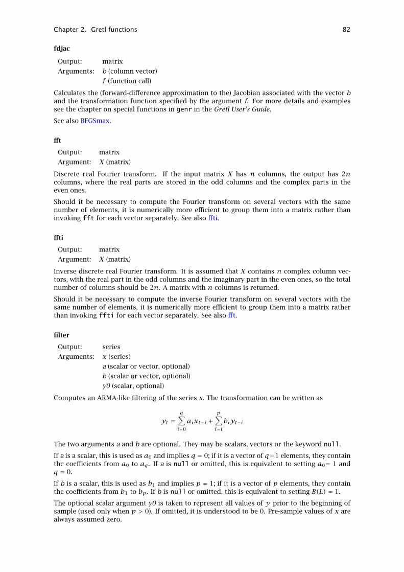
Chapter 2. Gretl functions 82
fdjac
Output: matrix
Arguments: b (column vector)
f (function call)
Calculates the (forward-difference approximation to the) Jacobian associated with the vector band the transformation function specified by the argument f. For more details and examplessee the chapter on special functions in genr in the Gretl User’s Guide.
See also BFGSmax.
fft
Output: matrix
Argument: X (matrix)
Discrete real Fourier transform. If the input matrix X has n columns, the output has 2ncolumns, where the real parts are stored in the odd columns and the complex parts in theeven ones.
Should it be necessary to compute the Fourier transform on several vectors with the samenumber of elements, it is numerically more efficient to group them into a matrix rather thaninvoking fft for each vector separately. See also ffti.
ffti
Output: matrix
Argument: X (matrix)
Inverse discrete real Fourier transform. It is assumed that X contains n complex column vec-tors, with the real part in the odd columns and the imaginary part in the even ones, so the totalnumber of columns should be 2n. A matrix with n columns is returned.
Should it be necessary to compute the inverse Fourier transform on several vectors with thesame number of elements, it is numerically more efficient to group them into a matrix ratherthan invoking ffti for each vector separately. See also fft.
filter
Output: series
Arguments: x (series)
a (scalar or vector, optional)
b (scalar or vector, optional)
y0 (scalar, optional)
Computes an ARMA-like filtering of the series x. The transformation can be written as
yt =q∑i=0
aixt−i +p∑i=ibiyt−i
The two arguments a and b are optional. They may be scalars, vectors or the keyword null.
If a is a scalar, this is used as a0 and implies q = 0; if it is a vector of q+1 elements, they containthe coefficients from a0 to aq. If a is null or omitted, this is equivalent to setting a0= 1 andq = 0.
If b is a scalar, this is used as b1 and implies p = 1; if it is a vector of p elements, they containthe coefficients from b1 to bp. If b is null or omitted, this is equivalent to setting B(L) = 1.
The optional scalar argument y0 is taken to represent all values of y prior to the beginning ofsample (used only when p > 0). If omitted, it is understood to be 0. Pre-sample values of x arealways assumed zero.
Chapter 2. Gretl functions 83
See also bkfilt, fracdiff, hpfilt, movavg.
Example:
nulldata 5y = filter(index, 0.5, -0.9, 1)print index y --byobs
produces
index y
1 1 -0.400002 2 1.360003 3 0.276004 4 1.751605 5 0.92356
firstobs
Output: scalar
Argument: y (series)
First non-missing observation for the variable y. Note that if some form of subsampling is ineffect, the value returned may be smaller than the dollar variable $t1. See also lastobs.
floor
Output: same type as input
Argument: y (scalar, series or matrix)
Floor function: returns the greatest integer less than or equal to x. Note: int and floor differin their effect for negative arguments: int(-3.5) gives −3, while floor(-3.5) gives −4.
fracdiff
Output: series
Arguments: y (series)
d (scalar)
∆dyt = yt − ∞∑i=1
ψiyt−i
where
ψi =Γ(i− d)Γ(−d)Γ(i+ 1)
Note that in theory fractional differentiation is an infinitely long filter. In practice, presamplevalues of yt are assumed to be zero.
gammafun
Output: same type as input
Argument: x (scalar, series or matrix)
Returns the gamma function of x.

Chapter 2. Gretl functions 84
getenv
Output: string
Argument: s (string)
If an environment variable by the name of s is defined, returns the value of that variable, other-wise returns an empty string.
gini
Output: scalar
Argument: y (series)
Returns Gini’s inequality index for the series y.
ginv
Output: matrix
Argument: A (matrix)
Returns A+, the Moore–Penrose or generalized inverse of A, computed via the singular valuedecomposition.
This matrix has the properties
AA+A = AA+AA+ = A+
Moreover, the products A+A and AA+ are symmetric by construction.
See also inv, svd.
hpfilt
Output: series
Arguments: y (series)
lambda (scalar, optional)
Returns the cycle component from application of the Hodrick–Prescott filter to series y. If thesmoothing parameter, lambda, is not supplied then a data-based default is used; the defaultcan also be adjusted using the set command. See the Gretl User’s Guide for details. See alsobkfilt.
I
Output: square matrix
Argument: n (scalar)
Returns an identity matrix with n rows and columns.
imaxc
Output: row vector
Argument: X (matrix)
Returns the row indices of the maxima of the columns of X.
See also imaxr, iminc, maxc.

Chapter 2. Gretl functions 85
imaxr
Output: column vector
Argument: X (matrix)
Returns the column indices of the maxima of the rows of X.
See also imaxc, iminr, maxr.
imhof
Output: scalar
Arguments: M (matrix)
x (scalar)
Computes Prob(u′Au < x) for a quadratic form in standard normal variates, u, using theprocedure developed by Imhof (1961).
If the first argument, M, is a square matrix it is taken to specify A, otherwise if it’s a columnvector it is taken to be the precomputed eigenvalues of A, otherwise an error is flagged.
See also pvalue.
iminc
Output: row vector
Argument: X (matrix)
Returns the row indices of the minima of the columns of X.
See also iminr, imaxc, minc.
iminr
Output: column vector
Argument: X (matrix)
Returns the column indices of the mimima of the rows of X.
See also iminc, imaxr, minr.
infnorm
Output: scalar
Argument: X (matrix)
Returns the ∞-norm of the r × c matrix X, namely,
‖X‖∞ =maxi
c∑j=1
|Xij|
See also onenorm.
int
Output: same type as input
Argument: x (scalar, series or matrix)
Returns the integer part of x, truncating the fractional part. Note: int and floor differ in theireffect for negative arguments: int(-3.5) gives −3, while floor(-3.5) gives −4. See also ceil.

Chapter 2. Gretl functions 86
inv
Output: matrix
Argument: A (square matrix)
Returns the inverse of A. If A is singular or not square, an error message is produced andnothing is returned. Note that gretl checks automatically the structure of A and uses the mostefficient numerical procedure to perform the inversion.
The matrix types gretl checks for are: identity; diagonal; symmetric and positive definite; sym-metric but not positive definite; and triangular.
See also ginv, invpd.
invcdf
Output: same type as input
Arguments: c (character)
. . . (see below)
p (scalar, series or matrix)
Inverse cumulative distribution function calculator. Returns x such that P(X ≤ x) = p, wherethe distribution X is determined by the character c; Between the arguments c and p, zero ormore additional scalar arguments are required to specify the parameters of the distribution, asfollows.
Distribution code, c Arg 2 Arg 3
Standard normal z, n or N – –
Student’s t (central) t degrees of freedom –
Chi square c, x or X degrees of freedom –
Snedecor’s F f or F df (num.) df (den.)
Binomial b or B p n
See also cdf, critical, pvalue.
invpd
Output: square matrix
Argument: A (symmetric matrix)
Returns the inverse of the symmetric, positive definite matrix A. This function is slightly fasterthan inv for large matrices, since no check for symmetry is performed; for that reason it shouldbe used with care.
irr
Output: scalar
Argument: x (series or vector)
Returns the Internal Rate of Return for x, considered as a sequence of payments (negative) andreceipts (positive). See also npv.
islist
Output: scalar
Argument: s (string)
Returns 1 if s is the identifier for a currently defined list, otherwise 0. See also isnull, isseries,isstring.

Chapter 2. Gretl functions 87
isnull
Output: scalar
Argument: s (string)
Returns 0 if s is the identifier for a currently defined object, be it a scalar, a series, a matrix, listor string; otherwise returns 1. See also islist, isseries, isstring.
kdensity
Output: matrix
Arguments: x (series)
scale (scalar, optional)
control (scalar, optional)
Computes a kernel density estimate for the series x. The returned matrix has two columns, thefirst holding a set of evenly spaced abscissae and the second the estimated density at each ofthese points.
The optional scale parameter can be used to adjust the degree of smoothing relative to thedefault of 1.0 (higher values produce a smoother result). The control parameter acts as aboolean: 0 (the default) means that the Gaussian kernel is used; a non-zero value switches tothe Epanechnikov kernel.
A plot of the results may be obtained using the gnuplot command, as in
matrix d = kdensity(x)gnuplot 2 1 --matrix=d --with-lines
kfilter
Output: scalar
Arguments: &E (reference to matrix, or null)
&V (reference to matrix, or null)
&S (reference to matrix, or null)
&P (reference to matrix, or null)
&G (reference to matrix, or null)
Requires that a Kalman filter be set up. Performs a forward, filtering pass and returns 0 onsuccessful completion or 1 if numerical problems are encountered.
The optional matrix arguments can be used to retrieve the following information: E gets thematrix of one-step ahead prediction errors and V gets the variance matrix for these errors;S gets the matrix of estimated values of the state vector and P the variance matrix of theseestimates; G gets the Kalman gain. All of these matrices have T rows, corresponding to Tobservations. For the column dimensions and further details see the Gretl User’s Guide.
See also kalman, ksmooth, ksimul.
ksimul
Output: matrix
Arguments: v (matrix)
w (matrix)
&S (reference to matrix, or null)
Requires that a Kalman filter be set up. Performs a simulation and returns a matrix holdingsimulated values of the observable variables.

Chapter 2. Gretl functions 88
The argument v supplies artificial disturbances for the state transition equation and w suppliesdisturbances for the observation equation, if applicable. The optional argument S may be usedto retrieve the simulated state vector. For details see the Gretl User’s Guide.
See also kalman, kfilter, ksimul.
ksmooth
Output: matrix
Argument: &P (reference to matrix, or null)
Requires that a Kalman filter be set up. Performs a backward, smoothing pass and returns amatrix holding smoothed estimates of the state vector. The optional argument P may be usedto retrieve the MSE of the smoothed state. For details see the Gretl User’s Guide.
See also kalman, kfilter, ksimul.
isseries
Output: scalar
Argument: s (string)
Returns 1 if s is the identifier for a currently defined series, otherwise 0. See also islist, isnull,isstring.
isstring
Output: scalar
Argument: s (string)
Returns 1 if s is the identifier for a currently defined string, otherwise 0. See also islist, isnull,isseries.
lags
Output: list
Arguments: p (scalar)
y (series or list)
Generates lags 1 to p of the series y, or if y is a list, of all variables in the list. If p = 0, themaximum lag defaults to the periodicity of the data; otherwise p must be positive.
The generated variables are automatically named according to the template varname_i wherevarname is the name of the original series and i is the specific lag. The original portion of thename is truncated if necessary, and may be adjusted in case of non-uniqueness in the set ofnames thus constructed.
lastobs
Output: scalar
Argument: y (series)
Last non-missing observation for the variable y. Note that if some form of subsampling is ineffect, the value returned may be larger than the dollar variable $t2. See also firstobs.
ldet
Output: scalar
Argument: A (square matrix)
Returns the natural log of the determinant of A, computed via the LU factorization. See alsodet, rcond.

Chapter 2. Gretl functions 89
ldiff
Output: same type as input
Argument: y (series or list)
Computes log differences; starting values are set to NA.
When a list is returned, the individual variables are automatically named according to the tem-plate ld_varname where varname is the name of the original series. The name is truncated ifnecessary, and may be adjusted in case of non-uniqueness in the set of names thus constructed.
See also diff, sdiff.
lincomb
Output: series
Arguments: L (list)
b (vector)
Computes a new series as a linear combination of the series in the list L. The coefficients aregiven by the vector b, which must have length equal to the number of series in L.
See also wmean.
ljungbox
Output: scalar
Arguments: y (series)
p (scalar)
Computes the Ljung–Box Q’ statistic for the series y using lag order p. The currently definedsample range is used. The lag order must be greater than or equal to 1 and less than the numberof available observations.
This statistic may be referred to the chi-square distribution with p degrees of freedom as a testof the null hypothesis that the series y is serially independent. See also pvalue.
lngamma
Output: same type as input
Argument: x (scalar, series or matrix)
Returns the log of the gamma function of x.
log
Output: same type as input
Argument: x (scalar, series, matrix or list)
Returns the natural logarithm of x ; produces NA for non-positive values. Note: ln is an accept-able alias for log.
When a list is returned, the individual variables are automatically named according to the tem-plate l_varname where varname is the name of the original series. The name is truncated ifnecessary, and may be adjusted in case of non-uniqueness in the set of names thus constructed.
log10
Output: same type as input
Argument: x (scalar, series or matrix)
Returns the base-10 logarithm of x ; produces NA for non-positive values.

Chapter 2. Gretl functions 90
log2
Output: same type as input
Argument: x (scalar, series or matrix)
Returns the base-2 logarithm of x ; produces NA for non-positive values.
logistic
Output: same type as input
Argument: x (scalar, series or matrix)
Returns the logistic function of the argument x, that is, Λ(x) = ex/(1+ ex). If x is a matrix, thefunction is applied element by element.
lower
Output: square matrix
Argument: A (matrix)
Returns an n×n lower triangular matrix B for which Bij = Aij if i ≥ j, and 0 otherwise.
See also upper.
lrvar
Output: scalar
Arguments: y (series)
k (scalar)
Returns the long-run variance of y, calculated using a Bartlett kernel with window size k. If k isnegative, int(T^(1/3)) is used.
In formulae:
ω2(k) = 1T
T−k∑t=k
k∑i=−k
wi(yt − X)(yt−i − Y )
with
wi = 1− |i|k+ 1
makemask
Output: column vector
Argument: y (series)
Produces a column vector containing the observation numbers corresponding to the non-zeroentries in the series y. This function is typically useful for filtering out rows of a matrix builtfrom data series.
max
Output: scalar or series
Argument: y (series or list)
If the argument y is a series, returns the (scalar) maximum of the non-missing observations inthe series. If the argument is a list, returns a series each of whose elements is the maximum ofthe values of the listed variables at the given observation.
See also min, xmax, xmin.

Chapter 2. Gretl functions 91
maxc
Output: row vector
Argument: X (matrix)
Returns a row vector containing the maxima of the columns of X.
See also imaxc, maxr, minc.
maxr
Output: column vector
Argument: X (matrix)
Returns a column vector containing the maxima of the rows of X.
See also imaxc, maxc, minr.
mcorr
Output: matrix
Argument: X (matrix)
Computes a correlation matrix treating each column of X as a variable. See also corr, cov, mcov.
mcov
Output: matrix
Argument: X (matrix)
Computes a covariance matrix treating each column of X as a variable. See also corr, cov, mcorr.
mcovg
Output: matrix
Arguments: X (matrix)
u (vector, optional)
w (vector, optional)
p (scalar)
Returns the matrix covariogram for a T × k matrix X (typically containing regressors), an (op-tional) T -vector u (typically containing residuals), an (optional) (p+1)-vector of weights w, and ascalar lag order p, which must be greater than or equal to 0.
The returned matrix is given by
p∑j=−p
∑jw|j|(X′tutut−jXt−j)
If u is given as null the u terms are omitted, and if w is given as null all the weights are takento be 1.0.
mean
Output: scalar or series
Argument: x (series or list)
If x is a series, returns the (scalar) sample mean, skipping any missing observations.
If x is a list, returns a series y such that yt is the mean of the values of the variables in the listat observation t, or NA if there are any missing values at t.

Chapter 2. Gretl functions 92
meanc
Output: row vector
Argument: X (matrix)
Returns the means of the columns of X. See also meanr, sumc, sdc.
meanr
Output: column vector
Argument: X (matrix)
Returns the means of the rows of X. See also meanc, sumr.
median
Output: scalar
Argument: y (series)
The median of the non-missing observations in series y. See also quantile.
mexp
Output: square matrix
Argument: A (square matrix)
Matrix exponential,
eA =∞∑k=0
Ak
k!= I
0!+ A
1!+ A
2
2!+ A
3
3!+ · · ·
(This series is sure to converge.) The algorithm used is 11.3.1 from Golub and Van Loan (1996).
min
Output: scalar or series
Argument: y (series or list)
If the argument y is a series, returns the (scalar) minimum of the non-missing observations inthe series. If the argument is a list, returns a series each of whose elements is the minimum ofthe values of the listed variables at the given observation.
See also max, xmax, xmin.
minc
Output: row vector
Argument: X (matrix)
Returns the minima of the columns of X.
See also iminc, maxc, minr.
minr
Output: column vector
Argument: X (matrix)
Returns the minima of the rows of X.
See also iminr, maxr, minc.

Chapter 2. Gretl functions 93
missing
Output: same type as input
Argument: x (scalar, series or list)
Returns a binary variable holding 1 if x is NA. If x is a series, the comparison is done elementby element; if x is a list of series, the output is a series with 1 at observations for which at leastone series in the list has a missing value, and 0 otherwise.
See also misszero, ok, zeromiss.
misszero
Output: same type as input
Argument: x (scalar or series)
Converts NAs to zeros. If x is a series, the conversion is done element by element. See alsomissing, ok, zeromiss.
mlag
Output: matrix
Arguments: X (matrix)
p (scalar or vector)
Shifts up or down the rows of X. If p is a positive scalar, the returned matrix Y has typicalelement Yi,j = Xi−p,j for i ≥ p and zero otherwise. In other words, the columns of X are shifteddown by p rows and the first p rows are filled with zeros. If p is a negative number, X is shiftedup and the last rows are filled with zeros.
If p is a vector, the above operation is carried out for each element in p, joining the resultingmatrices horizontally.
mnormal
Output: matrix
Arguments: r (scalar)
c (scalar)
Returns a matrix with r rows and c columns, filled with standard normal pseudo-random vari-ates. See also normal, muniform.
mols
Output: matrix
Arguments: Y (matrix)
X (matrix)
&U (reference to matrix, or null)
&V (reference to matrix, or null)
Returns a k×n matrix of parameter estimates obtained by OLS regression of the T ×n matrixY on the T × k matrix X.
If the third argument is not null, the T × n matrix U will contain the residuals. If the finalargument is given and is not null then the k×k matrix V will contain (a) the covariance matrixof the parameter estimates, if Y has just one column, or (b) X′X−1 if Y has multiple columns.
By default, estimates are obtained via Cholesky decomposition, with a fallback to QR decompo-sition if the columns of X are highly collinear. The use of SVD can be forced via the commandset svd on.

Chapter 2. Gretl functions 94
movavg
Output: series
Arguments: x (series)
p (scalar)
control (scalar, optional)
Depending on the value of the parameter p, returns either a simple or an exponentially weightedmoving average of the input series x.
If p > 1, a simple p-term moving average is computed, that is, 1p∑p−1i=0 xt−i. If a non-zero value
is supplied for the optional control parameter the MA is centered, otherwise it is “trailing”.
If 0 < p < 1, an exponential moving average is computed: yt = pxt + (1 − p)yt−1. By defaultthe output series y is initialized using the first valid value of x, but the control parameter maybe used to specify the number of initial observations that should be averaged to produce y0. Azero value for control indicates that all the observations should be used.
mpols
Output: matrix
Arguments: Y (matrix)
X (matrix)
&U (reference to matrix, or null)
Works exactly as mols, except that the calculations are done in multiple precision using theGMP library (assuming this is available).
By default GMP uses 256 bits for each floating point number, but you can adjust this using theenvironment variable GRETL_MP_BITS, e.g. GRETL_MP_BITS=1024.
mread
Output: matrix
Argument: s (string)
Reads a matrix from a text file. The string s must contain the name of the (plain text) file fromwhich the matrix is to be read. The file in question must conform to the following rules:
• The columns must be separated by spaces or tab characters.
• The decimal separator must be the dot character, “.”.
• The first line in the file must contain two integers, separated by a space or a tab, indicatingthe number of rows and columns, respectively.
Should an error occur (such as the file being badly formatted or inaccessible), an empty matrixis returned.
See also mwrite.
mreverse
Output: matrix
Argument: X (matrix)
Returns a matrix containing the rows of X in reverse order. If you wish to obtain a matrix inwhich the columns of X appear in reverse order you can do:
matrix Y = mreverse(X’)’
Chapter 2. Gretl functions 95
mshape
Output: matrix
Arguments: X (matrix)
r (scalar)
c (scalar)
Rearranges the elements of X into a matrix with r rows and c columns. Elements are read fromX and written to the target in column-major order. If X contains fewer than k = rc elements, theelements are repeated cyclically; otherwise, if X has more elements, only the first k are used.
See also cols, rows, unvech, vec, vech.
msortby
Output: matrix
Arguments: X (matrix)
j (scalar)
Returns a matrix in which the rows of X are reordered by increasing value of the elements incolumn j.
muniform
Output: matrix
Arguments: r (scalar)
c (scalar)
Returns a matrix with r rows and c columns, filled with uniform (0,1) pseudo-random variates.Note: the preferred method for generating a scalar uniform r.v. is recasting the output ofmuniform to a scalar, as in
scalar x = muniform(1,1)
See also mnormal, uniform.
mwrite
Output: scalar
Arguments: X (matrix)
s (string)
Writes the matrix X to a plain text file named s. The file will contain on the first line twointegers, separated by a tab character, with the number of rows and columns; on the next lines,the matrix elements in scientific notation, separated by tabs (one line per row).
If file s already exists, it will be overwritten. The return value is 0 on successful completion; ifan error occurs, such as the file being unwritable, the return value will be non-zero.
Matrices stored via the mwrite command can be easily read by other programs; see the GretlUser’s Guide for details.
See also mread.
mxtab
Output: matrix
Arguments: x (series or vector)
y (series or vector)

Chapter 2. Gretl functions 96
Returns a matrix holding the cross tabulation of the values contained in x (by row) and y (bycolumn). The two arguments should be of the same type (both series or both column vectors),and because of the typical usage of this function, are assumed to contain integer values only.
See also values.
nelem
Output: scalar
Argument: L (list)
Returns the number of items in list L.
nobs
Output: scalar
Argument: y (series)
Returns the number of non-missing observations for the variable y in the currently selectedsample.
normal
Output: series
Arguments: µ (scalar)
σ (scalar)
Generates a series of Gaussian pseudo-random variates with mean µ and standard deviation σ .If no arguments are supplied, standard normal variates N(0,1) are produced. The values areproduced using the Ziggurat method (Marsaglia and Tsang, 2000).
See also randgen, mnormal, muniform.
npv
Output: scalar
Arguments: x (series or vector)
r (scalar)
Returns the Net Present Value of x, considered as a sequence of payments (negative) and re-ceipts (positive), evaluated at annual discount rate r. The first value is taken as dated “now”and is not discounted. To emulate an NPV function in which the first value is discounted,prepend zero to the input sequence.
Supported data frequencies are annual, quarterly, monthly, and undated (undated data aretreated as if annual).
See also irr.
nullspace
Output: matrix
Argument: A (matrix)
Computes the right nullspace of A, via the singular value decomposition: the result is a matrixB such that AB = [0], except when A has full column rank, in which case an empty matrix isreturned. Otherwise, if A is m×n, B will be an n× (n− r) matrix, where r is the rank of A.
See also rank, svd.

Chapter 2. Gretl functions 97
obs
Output: series
Returns a series of consecutive integers, setting 1 at the start of the dataset. Note that the resultis invariant to subsampling. This function is especially useful with time-series datasets. Note:you can write t instead of obs with the same effect.
See also obsnum.
obslabel
Output: string
Argument: t (scalar)
Returns the observation label for observation t, where t is a 1-based index. The inverse functionis provided by obsnum.
obsnum
Output: scalar
Argument: s (string)
Returns an integer corresponding to the observation specified by the string s. Note that theresult is invariant to subsampling. This function is especially useful with time-series datasets.For example, the following code
open denmarkk = obsnum(1980:1)
yields k = 25, indicating that the first quarter of 1980 is the 25th observation in the denmarkdataset.
See also obs, obslabel.
ok
Output: same type as input
Argument: x (scalar, series or list)
Returns a binary variable holding 1 if x is not NA. If x is a series, the comparison is done elementby element. If x is a list of series, the output is a series with 0 at observations for which at leastone series in the list has a missing value, and 1 otherwise.
See also missing, misszero, zeromiss.
onenorm
Output: scalar
Argument: X (matrix)
Returns the 1-norm of the r × c matrix X :
‖X‖1 =maxj
r∑i=1
|Xij|
See also infnorm, rcond.

Chapter 2. Gretl functions 98
ones
Output: matrix
Arguments: r (scalar)
c (scalar)
Outputs a matrix with r rows and c columns, filled with ones.
See also seq, zeros.
orthdev
Output: series
Argument: y (series)
Only applicable if the currently open dataset has a panel structure. Computes the forwardorthogonal deviations for variable y, that is
yi,t =√
Ti − tTi − t + 1
yi,t − 1Ti − t
Ti∑s=t+1
yi,s
This transformation is sometimes used instead of differencing to remove individual effects frompanel data. For compatibility with first differences, the deviations are stored one step ahead oftheir true temporal location (that is, the value at observation t is the deviation that, strictlyspeaking, belongs at t − 1). That way one loses the first observation in each time series, not thelast.
See also diff.
Output: same type as input
Arguments: c (character)
. . . (see below)
x (scalar, series or matrix)
Examples: f1 = pdf(N, -2.5)
f2 = pdf(X, 3, y)
f3 = pdf(W, shape, scale, y)
Probability density function calculator. Returns the density at x of the distribution identified bythe code c. See cdf for details of the required (scalar) arguments. The distributions supportedby the pdf function are the normal, Student’s t, chi-square, F , Gamma and Weibull.
For the normal distribution, see also dnorm.
pergm
Output: matrix
Arguments: x (series or vector)
bandwidth (scalar, optional)
If only the first argument is given, computes the sample periodogram for the given series or vec-tor. If the second argument is given, computes an estimate of the spectrum of x using a Bartlettlag window of the given bandwidth, up to a maximum of half the number of observations (T/2).
Returns a matrix with two columns and T/2 rows: the first column holds the frequency, ω,from 2π/T to π , and the second the corresponding spectral density.
pmax
Output: series
Argument: y (series)

Chapter 2. Gretl functions 99
Only applicable if the currently open dataset has a panel structure. Returns the per-unit maxi-mum for variable y.
Missing values are skipped. See also pmin, pmean, pnobs, psd.
pmean
Output: series
Argument: y (series)
Only applicable if the currently open dataset has a panel structure. Computes the per-unit meanfor variable y ; that is,
yi =1Ti
Ti∑t=1
yi,t
where Ti is the number of valid observations for unit i.
Missing values are skipped. See also pmax, pmin, pnobs, psd.
pmin
Output: series
Argument: y (series)
Only applicable if the currently open dataset has a panel structure. Returns the per-unit mini-mum for variable y.
Missing values are skipped. See also pmax, pmean, pnobs, psd.
pnobs
Output: series
Argument: y (series)
Only applicable if the currently open dataset has a panel structure. Returns for each unit thenumber of non-missing cases for the variable y.
Missing values are skipped. See also pmax, pmin, pmean, psd.
polroots
Output: matrix
Argument: a (vector)
Finds the roots of a polynomial. If the polynomial is of degree p, the vector a should contain p +1 coefficients in ascending order, i.e. starting with the constant and ending with the coefficienton xp.
If all the roots are real they are returned in a column vector of length p, otherwise a p×2 matrixis returned, the real parts in the first column and the imaginary parts in the second.
princomp
Output: matrix
Arguments: X (matrix)
p (scalar)
Let the matrix X be T × k, containing T observations on k variables. The argument p must bea positive integer less than or equal to k. This function returns a T × p matrix, P , holding thefirst p principal components of X.

Chapter 2. Gretl functions 100
The elements of P are computed as
Ptj =k∑i=1
Zti v(j)i
where Zti is the standardized value of variable i at observation t, Zti = (Xti − Xi)/σi, and v(j)is the jth eigenvector of the correlation matrix of the Xis, with the eigenvectors ordered bydecreasing value of the corresponding eigenvalues.
See also eigensym.
psd
Output: series
Argument: y (series)
Only applicable if the currently open dataset has a panel structure. Computes the per-unitsample standard deviation for variable y , that is
σi =
√√√√√ 1Ti − 1
Ti∑t=1
(yi,t − yi)2
The above formula holds for Ti ≥ 2, where Ti is the number of valid observations for unit i; ifTi = 0, NA is returned; if Ti = 1, 0 is returned.
Note: this function makes it possible to check whether a given variable (say, X) is time-invariantvia the condition max(psd(X)) = 0.
See also pmax, pmin, pmean, pnobs.
psdroot
Output: square matrix
Argument: A (symmetric matrix)
Performs a generalized variant of the Cholesky decomposition of the matrix A, which must bepositive semidefinite (but which may be singular). If the input matrix is not square an erroris flagged, but symmetry is assumed and not tested; only the lower triangle of A is read. Theresult is a lower-triangular matrix L which satisfies A = LL′. Indeterminate elements in thesolution are set to zero.
For the case where A is positive definite, see cholesky.
pvalue
Output: same type as input
Arguments: c (character)
. . . (see below)
x (scalar, series or matrix)
Examples: p1 = pvalue(z, 2.2)
p2 = pvalue(X, 3, 5.67)
p2 = pvalue(F, 3, 30, 5.67)
P -value calculator. Returns P(X > x), where the distribution X is determined by the characterc. Between the arguments c and x, zero or more additional arguments are required to specifythe parameters of the distribution; see cdf for details. The distributions supported by the pvalfunction are the standard normal, t, Chi square, F , gamma, binomial, Poisson and Weibull.
See also critical, invcdf, urcpval, imhof.

Chapter 2. Gretl functions 101
qform
Output: matrix
Arguments: x (matrix)
A (symmetric matrix)
Computes the quadratic form Y = xAx′. Using this function instead of ordinary matrix multi-plication guarantees more speed and better accuracy. If x and A are not conformable, or A isnot symmetric, an error is returned.
qnorm
Output: same type as input
Argument: x (scalar, series or matrix)
Returns quantiles for the standard normal distribution. If x is not between 0 and 1, NA isreturned. See also cnorm, dnorm.
qrdecomp
Output: matrix
Arguments: X (matrix)
&R (reference to matrix, or null)
Computes the QR decomposition of an m × n matrix X, that is X = QR where Q is an m × northogonal matrix and R is an n×n upper triangular matrix. The matrix Q is returned directly,while R can be retrieved via the optional second argument.
See also eigengen, eigensym, svd.
quantile
Output: scalar or row vector
Arguments: y (series or matrix)
p (scalar between 0 and 1)
Given a series argument, returns the p-quantile for the series. For example, when p = 0.5, themedian is returned. Given a matrix argument, returns a row vector containing the p-quantilesfor the columns of y ; that is, each column is treated as a series.
For a series of length n, the p-quantile, q, is defined as:
q = y[k] + (n · p − k)(y[k+1] −y[k])
where k is the integer part of n · p and y[i] is the i-th element of the series when sorted fromsmallest to largest.
rank
Output: scalar
Argument: X (matrix)
Returns the rank of X, numerically computed via the singular value decomposition. See alsosvd.
ranking
Output: series
Argument: y (series)
Returns a series with the ranks of y . The rank for observation i is the number of elements inthe series that are less than yi plus one half the number of elements in the series that are equal

Chapter 2. Gretl functions 102
to yi. (Intuitively, you may think of chess points, where victory gives you one point and a drawgives you half a point.) One is added so the lowest rank is 1 instead of 0.
Formally,rank(yi) = 1+
∑j 6=i
[I(yj < yi)+ 0.5 · I(yj = yi)
]where I denotes the indicator function.
See also sort, sortby.
randgen
Output: series
Arguments: c (character)
a (scalar or series)
b (scalar or series)
Examples: series x = randgen(u, 0, 100)
series t14 = randgen(t, 14)
series y = randgen(B, 0.6, 30)
series g = randgen(G, 1, 1)
series P = randgen(P, mu)
All-purpose random number generator. The parameter c is a character, which specifies fromwhich distribution the pseudo-random numbers should be drawn. The arguments a and (insome cases) b provide the parameters of the selected distribution. If these are given as scalarsthe output series is identically distributed; if a series is given for a or b the distribution isconditional on the parameter value at each observation.
Specifics are given below: the character codes for each distribution are shown in parentheses,followed by the interpretation of the argument a and, where applicable, b.
Distribution c a b
Uniform (continuous) u or U minimum maximum
Normal z, n or N mean standard deviation
Student’s t t degrees of freedom –
Chi square c, x or X degrees of freedom –
Snedecor’s F f or F df (num.) df (den.)
Gamma g or G shape scale
Binomial b or B p nPoisson p or P mean –
Weibull w or W shape scale
See also normal, uniform.
rcond
Output: scalar
Argument: A (square matrix)
Returns the reciprocal condition number for A with respect to the 1-norm. In many circum-stances, this is a better measure of the sensitivity of A to numerical operations such as inversionthan the determinant.
Given that A is non-singular, we may define
κ(A) = ||A||1 · ||A−1||1This function returns κ(A)−1.
See also det, ldet, onenorm.

Chapter 2. Gretl functions 103
readfile
Output: string
Argument: fname (string)
If a file by the name of fname exists and is readable, returns a string containing the content ofthis file, otherwise flags an error.
Also see the sscanf command.
replace
Output: same type as input
Arguments: x (series or matrix)
find (scalar or vector)
subst (scalar or vector)
Replaces each element of x equal to the i-th element of find with the corresponding element ofsubst.
If find is a scalar, subst must also be a scalar. If find and subst are both vectors, they musthave the same number of elements. But if find is a vector and subst a scalar, then all matcheswill be replaced by subst.
Example:
a = {1,2,3;3,4,5}find = {1,3,4}subst = {-1,-8, 0}b = replace(a, find, subst)print a b
produces
a (2 x 3)
1 2 33 4 5
b (2 x 3)
-1 2 -8-8 0 5
resample
Output: same type as input
Arguments: x (series or matrix)
b (scalar, optional)
Resamples from x with replacement. In the case of a series argument, each value of the returnedseries, yt , is drawn from among all the values of xt with equal probability. When a matrixargument is given, each row of the returned matrix is drawn from the rows of x with equalprobability.
The optional argument b represents the block length for resampling by moving blocks. If thisargument is given it should be a positive integer greater than or equal to 2. The effect is thatthe output is composed by random selection with replacement from among all the possible con-tiguous sequences of length b in the input. (In the case of matrix input, this means contiguousrows.) If the length of the data is not an integer multiple of the block length, the last selectedblock is truncated to fit.

Chapter 2. Gretl functions 104
round
Output: same type as input
Argument: x (scalar, series or matrix)
Rounds to the nearest integer. Note that when x lies halfway between two integers, roundingis done "away from zero", so for example 2.5 rounds to 3, but round(-3.5) gives −4. This isa common convention in spreadsheet programs, but other software may yield different results.See also ceil, floor, int.
rows
Output: scalar
Argument: X (matrix)
Number of rows of the matrix X. See also cols, mshape, unvech, vec, vech.
sd
Output: scalar or series
Argument: x (series or list)
If x is a series, returns the (scalar) sample standard deviation, skipping any missing observa-tions.
If x is a list, returns a series y such that yt is the sample standard deviation of the values ofthe variables in the list at observation t, or NA if there are any missing values at t.
See also var.
sdc
Output: row vector
Argument: X (matrix)
Returns the standard deviations of the columns of X (with no degrees of freedom correction).See also meanc, sumc.
sdiff
Output: same type as input
Argument: y (series or list)
Computes seasonal differences: yt −yt−k, where k is the periodicity of the current dataset (see$pd). Starting values are set to NA.
When a list is returned, the individual variables are automatically named according to the tem-plate sd_varname where varname is the name of the original series. The name is truncated ifnecessary, and may be adjusted in case of non-uniqueness in the set of names thus constructed.
See also diff, ldiff.
selifc
Output: matrix
Arguments: A (matrix)
b (row vector)
Selects from A only the columns for which the corresponding element of b is non-zero. b mustbe a row vector with the same number of columns as A.
See also selifr.

Chapter 2. Gretl functions 105
selifr
Output: matrix
Arguments: A (matrix)
b (column vector)
Selects from A only the rows for which the corresponding element of b is non-zero. b must bea column vector with the same number of rows as A.
See also selifc, trimr.
seq
Output: row vector
Arguments: a (scalar)
b (scalar)
k (scalar, optional)
Given only two arguments, returns a row vector filled with consecutive integers, with a as firstelement and b last. If a is greater than b the sequence will be decreasing. If either argument isnot integral its fractional part is discarded.
If the third argument is given, returns a row vector containing a sequence of integers startingwith a and incremented (or decremented, if a is greater than b) by k at each step. The finalvalue is the largest member of the sequence that is less than or equal to b (or mutatis mutandisfor a greater than b). The argument k must be positive; if it is not integral its fractional part isdiscarded.
See also ones, zeros.
sin
Output: same type as input
Argument: x (scalar, series or matrix)
Returns the sine of x. See also cos, tan, atan.
sinh
Output: same type as input
Argument: x (scalar, series or matrix)
Returns the hyperbolic sine of x.
sinhx = ex − e−x
2
See also asinh, cosh, tanh.
sort
Output: same type as input
Argument: x (series or vector)
Sorts x in ascending order, skipping observations with missing values when x is a series. Seealso dsort, values. For matrices specifically, see msortby.
sortby
Output: series
Arguments: y1 (series)
y2 (series)

Chapter 2. Gretl functions 106
Returns a series containing the elements of y2 sorted by increasing value of the first argument,y1. See also sort, ranking.
sqrt
Output: same type as input
Argument: x (scalar, series or matrix)
Returns the positive square root of x ; produces NA for negative values.
Note that if the argument is a matrix the operation is performed element by element and, sincematrices cannot contain NA, negative values generate an error. For the “matrix square root” seecholesky.
sscanf
Output: scalar
Arguments: src (string)
format (string)
. . . (see below)
Reads values from src under the control of format and assigns these values to one or moretrailing arguments, indicated by the dots above. Returns the number of values assigned. Formore details see the sscanf command.
sst
Output: scalar
Argument: y (series)
Returns the sum of squared deviations from the mean for the non-missing observations inseries y. See also var.
strlen
Output: scalar
Argument: s (string)
Returns the number of characters in s.
strncmp
Output: scalar
Arguments: s1 (string)
s2 (string)
n (scalar, optional)
Compares the two string arguments and returns an integer less than, equal to, or greater thanzero if s1 is found, respectively, to be less than, to match, or be greater than s2, up to the firstn characters. If n is omitted the comparison proceeds as far as possible.
Note that if you just want to compare two strings for equality, that can be done without usinga function, as in if (s1 == s2) ...
strstr
Output: string
Arguments: s1 (string)
s2 (string)

Chapter 2. Gretl functions 107
Searches s1 for an occurrence of the string s2. If a match is found, returns a copy of the portionof s1 that starts with s2, otherwise returns an empty string.
sum
Output: scalar
Argument: y (series)
Returns the sum of the non-missing observations in series y.
sumc
Output: row vector
Argument: X (matrix)
Returns the sums of the columns of X. See also meanc, sumr.
sumr
Output: column vector
Argument: X (matrix)
Returns the sums of the rows of X. See also meanr, sumc.
svd
Output: row vector
Arguments: X (matrix)
&U (reference to matrix, or null)
&V (reference to matrix, or null)
Performs the singular values decomposition of the r × c matrix X:
X = U
σ1
σ2
. . .
σn,
V
where n =min(r , c). U is r ×n and V is n× c, with U ′U = I and VV ′ = I.The singular values are returned in a row vector. The left and/or right singular vectors U andV may be obtained by supplying non-null values for arguments 2 and 3, respectively. For anymatrix A, the code
s = svd(A, &U, &V)B = (U .* s) * V
should yield B identical to A (apart from machine precision).
See also eigengen, eigensym, qrdecomp.
tan
Output: same type as input
Argument: x (scalar, series or matrix)
Returns the tangent of x.

Chapter 2. Gretl functions 108
tanh
Output: same type as input
Argument: x (scalar, series or matrix)
Returns the hyperbolic tangent of x.
tanhx = e2x − 1e2x + 1
See also atanh, cosh, sinh.
toepsolv
Output: column vector
Arguments: c (vector)
r (vector)
b (vector)
Solves a Toeplitz system of linear equations, that is Tx = b where T is a square matrix whoseelement T i,j equals ci−j for i ≥ j and r j−i for i ≤ j. Note that the first elements of c and r mustbe equal, otherwise an error is returned. Upon successful completion, the function returns thevector x.
The algorithm used here takes advantage of the special structure of the matrix T , which makes itmuch more efficient than other unspecialized algorithms, especially for large problems. Warn-ing: in certain cases, the function may spuriously issue a singularity error when in fact thematrix T is nonsingular; this problem, however, cannot arise when T is positive definite.
tolower
Output: string
Argument: s (string)
Returns a copy of s in which any upper-case characters are converted to lower case.
tr
Output: scalar
Argument: A (square matrix)
Returns the trace of the square matrix A, that is, the sum of its diagonal elements. See alsodiag.
transp
Output: matrix
Argument: X (matrix)
Returns the transpose of X. Note: this is rarely used; in order to get the transpose of a matrix,in most cases you can just use the prime operator: X’.
trimr
Output: matrix
Arguments: X (matrix)
ttop (scalar)
tbot (scalar)

Chapter 2. Gretl functions 109
Returns a matrix that is a copy of X with ttop rows trimmed at the top and tbot rows trimmedat the bottom. The latter two arguments must be non-negative, and must sum to less than thetotal rows of X.
See also selifr.
uniform
Output: series
Arguments: a (scalar)
b (scalar)
Generates a series of uniform pseudo-random variates in the interval (a, b), or, if no argumentsare supplied, in the interval (0,1). The algorithm used is the Mersenne Twister by Matsumotoand Nishimura (1998).
See also randgen, normal, mnormal, muniform.
unvech
Output: square matrix
Arguments: v (vector)
b (scalar)
Returns an n×n symmetric matrix obtained by rearranging the elements of v . The number ofelements in v must be a triangular integer — i.e., a number k such that an integer n exists withthe property k = n(n+ 1)/2. This is the inverse of the function vech.
See also mshape.
upper
Output: square matrix
Argument: A (square matrix)
Returns an n×n upper triangular matrix B for which Bij = Aij if i ≤ j and 0 otherwise.
See also lower.
urcpval
Output: scalar
Arguments: tau (scalar)
n (scalar)
niv (scalar)
itv (scalar)
P -values for the test statistic from the Dickey–Fuller unit-root test and the Engle–Granger coin-tegration test, as per James MacKinnon (1996).
The arguments are as follows: tau denotes the test statistic; n is the number of observations(or 0 for an asymptotic result); niv is the number of potentially cointegrated variables whentesting for cointegration (or 1 for a univariate unit-root test); and itv is a code for the modelspecification: 1 for no constant, 2 for constant included, 3 for constant and linear trend, 4 forconstant and quadratic trend.
Note that if the test regression is “augmented” with lags of the dependent variable, then youshould give an n value of 0 to get an asymptotic result.
See also pvalue.

Chapter 2. Gretl functions 110
values
Output: column vector
Argument: x (series or vector)
Returns a vector containing the distinct elements of x sorted in ascending order. If you wish totruncate the values to integers before applying this function, use the expression values(int(x)).
See also dsort, sort.
var
Output: scalar or series
Argument: x (series or list)
If x is a series, returns the (scalar) sample variance, skipping any missing observations.
If x is a list, returns a series y such that yt is the sample variance of the values of the variablesin the list at observation t, or NA if there are any missing values at t.
In each case the sum of squared deviations from the mean is divided by (n − 1) for n > 1.Otherwise the variance is given as zero if n = 1, or as NA if n = 0.
See also sd.
varname
Output: string
Argument: v (scalar or list)
If given a scalar argument, returns the name of the variable with ID number v, or generates anerror if there is no such variable.
If given a list argument, returns a string containing the names of the variables in the list, sepa-rated by commas. If the supplied list is empty, so is the returned string.
varnum
Output: scalar
Argument: varname (string)
Returns the ID number of the variable called varname, or NA is there is no such variable.
vec
Output: column vector
Argument: X (matrix)
Stacks the columns of X as a column vector. See also mshape, unvech, vech.
vech
Output: column vector
Argument: A (square matrix)
Returns in a column vector the elements of A on and above the diagonal. Typically, this functionis used on symmetric matrices; in this case, it can be undone by the function unvech. See alsovec.
Chapter 2. Gretl functions 111
weekday
Output: scalar
Arguments: year (scalar)
month (scalar)
day (scalar)
Returns the day of the week (Sunday = 0, Monday = 1, etc.) for the date specified by the threearguments, or NA if the date is invalid.
wmean
Output: series
Arguments: Y (list)
W (list)
Returns a series y such that yt is the weighted mean of the values of the variables in list Yat observation t, the respective weights given by the values of the variables in list W at t. Theweights can therefore be time-varying. The lists Y and W must be of the same length and theweights must be non-negative.
See also wsd, wvar.
wsd
Output: series
Arguments: Y (list)
W (list)
Returns a series y such that yt is the weighted sample standard deviation of the values of thevariables in list Y at observation t, the respective weights given by the values of the variables inlist W at t. The weights can therefore be time-varying. The lists Y and W must be of the samelength and the weights must be non-negative.
See also wmean, wvar.
wvar
Output: series
Arguments: X (list)
W (list)
Returns a series y such that yt is the weighted sample variance of the values of the variablesin list X at observation t, the respective weights given by the values of the variables in list Wat t. The weights can therefore be time-varying. The lists Y and W must be of the same lengthand the weights must be non-negative.
The weighted sample variance is computed as
s2w =
n′
n′ − 1
∑ni=1wi(xi − xw)2∑n
i=1wi
where n′ is the number of non-zero weights and xw is the weighted mean.
See also wmean, wsd.
xmax
Output: scalar
Arguments: x (scalar)
y (scalar)
Returns the greater of x and y, or NA if either value is missing.
Chapter 2. Gretl functions 112
See also xmin, max, min.
xmin
Output: scalar
Arguments: x (scalar)
y (scalar)
Returns the lesser of x and y, or NA if either value is missing.
See also xmax, max, min.
xpx
Output: list
Argument: L (list)
Returns a list that references the squares and cross-products of the variables in list L. Squaresare named on the pattern sq_varname and cross-products on the pattern var1_var2. The inputvariable names are truncated if need be, and the output names may be adjusted in case ofduplication of names in the returned list.
zeromiss
Output: same type as input
Argument: x (scalar or series)
Converts zeros to NAs. If x is a series, the conversion is done element by element. See alsomissing, misszero, ok.
zeros
Output: matrix
Arguments: r (scalar)
c (scalar)
Outputs a zero matrix with r rows and c columns. See also ones, seq.

Chapter 3
Comments in scripts
When a script does anything non-obvious, it’s a good idea to add comments explaining what’sgoing on. This is particularly useful if you plan to share the script with others, but it’s alsouseful as a reminder to yourself — when you revisit a script some months later and wonderwhat it was supposed to be doing.
The comment mechanism can also be helpful when you’re developing a script. There maycome a point where you want to execute a script, but bypass execution of some portion of it.Obviously you could delete the portion you wish to bypass, but rather than lose that sectionyou can “comment it out” so that it is ignored by gretl.
Two sorts of comments are supported by gretl. The simpler one is this:
• If a hash mark, #, is encountered in a gretl script, everything from that point to the end ofthe current line is treated as a comment, and ignored.
If you wish to “comment out” several lines using this mode, you’ll have to place a hash mark atthe start of each line.
The second sort of comment is patterned after the C programming language:
• If the sequence /* is encountered in a script, all the following input is treated as a com-ment until the sequence */ is found.
Comments of this sort can extend over several lines. Using this mode it is easy to add lengthyexplanatory text, or to get gretl to ignore substantial blocks of commands. As in C, commentsof this type cannot be nested.
How do these two comment modes interact? You can think of gretl as starting at the top of ascript and trying to decide at each point whether it should or should not be in “ignore mode”.In doing so it follows these rules:
• If we’re not in ignore mode, then # puts us into ignore mode till the end of the currentline.
• If we’re not in ignore mode, then /* puts us into ignore mode until */ is found.
This means that each sort of comment can be masked by the other.
• If /* follows # on a given line which does not already start in ignore mode, then there’snothing special about /*, it’s just part of a #-style comment.
• If # occurs when we’re already in ignore mode, it is just part of a comment.
A few examples follow.
/* multi-line comment# hello# hello */
In the above example the hash marks are not special; in particular the hash mark on the thirdline does not prevent the multi-line comment from terminating at */.
113

Chapter 3. Comments in scripts 114
# single-line comment /* hello
Assuming we were not in ignore mode before the line shown above, it is just a single-linecomment: the /* is masked, and does not open a multi-line comment.
You can append a comment to a command:
ols 1 0 2 3 # estimate the baseline model
Example of “commenting out”:
/*# let’s skip this for nowols 1 0 2 3 4omit 3 4*/

Chapter 4
Options, arguments and path-searching
4.1 Invoking gretl
gretl (under MS Windows, gretlw32.exe)1.
— Opens the program and waits for user input.
gretl datafile
— Starts the program with the specified datafile in its workspace. The data file may be in anyof several formats (see the Gretl User’s Guide); the program will try to detect the format of thefile and treat it appropriately. See also Section 4.4 below for path-searching behavior.
gretl --help (or gretl -h)
— Print a brief summary of usage and exit.
gretl --version (or gretl -v)
— Print version identification for the program and exit.
gretl --english (or gretl -e)
— Force use of English instead of translation.
gretl --run scriptfile (or gretl -r scriptfile)
— Start the program and open a window displaying the specified script file, ready to run. SeeSection 4.4 below for path-searching behavior.
gretl --db database (or gretl -d database)
— Start the program and open a window displaying the specified database. If the database files(the .bin file and its accompanying .idx file) are not in the default system database directory,you must specify the full path. See also the Gretl User’s Guide for details on databases.
gretl --dump (or gretl -c)
— Dump the program’s configuration information to a plain text file (the name of the file isprinted on standard output). May be useful for trouble-shooting.
gretlw32 --debug (or gretlw32 -g)
— (MS Windows only) Open a console window to display any messages sent to the “standardoutput” or “standard error” streams. Such messages are not usually visible on Windows; thismay be useful for trouble-shooting.
4.2 Preferences dialog
Various things in gretl are configurable under the “Tools, Preferences” menu. Separate menuitems are devoted to the choice of the monospaced font to be used in gretl screen output,and, on some platforms, the font used for menus and other messages. The other options areorganized under five tabs, as follows.
General: Here you can configure the base directory for gretl’s shared files. In addition there areseveral check boxes. Checking “Tell me about gretl updates” makes gretl attempt to query theupdate server at start-up. If your native language setting is not English and the local decimal
1On Linux, a “wrapper” script named gretl is installed. This script checks whether the DISPLAY environmentvariable is set; if so, it launches the GUI program, gretl_x11, and if not it launches the command-line program,gretlcli
115
Chapter 4. Options, arguments and path-searching 116
point character is not the period (“.”), unchecking “Use locale setting for decimal point” willmake gretl use the period regardless. Checking “Allow shell commands” makes it possible toinvoke shell commands in scripts and in the gretl console (this facility is disabled by default forsecurity reasons).
Databases tab: You can select the directory in which to start looking for native gretl databases;the directory in which to start looking for RATS 4 databases; the host name of the gretl databaseserver to access; and the IP number and port number of the HTTP proxy server to use whencontacting the database server (if you’re behind a firewall).
Programs tab: You can specify the names or paths to various third-party programs that maycalled by gretl under certain conditions. Note that the item “Command to compile TEX files” canbe set to either latex or pdflatex; if latex is selected, TEX output will be previewed in DVI format;if pdflatex is selected, the preview will be in PDF format.
HCCME tab: Set preferences regarding robust covariance matrix estimation. See the Gretl User’sGuide for details.
Manuals tab: Select your preferred language for the full gretl documentation in PDF format(currently only English and Italian are supported). When using the English documentation youcan also choose between US letter paper and A4 paper.
Settings chosen via the Preferences dialog are stored from one gretl session to the next. UnderMS Windows they are stored in the Windows registry; on other platforms they are stored in aplain text file named .gretl2rc in the user’s home directory.
4.3 Invoking gretlcli
gretlcli
— Opens the program and waits for user input.
gretlcli datafile
— Starts the program with the specified datafile in its workspace. The data file may be in anyformat supported by gretl (see the Gretl User’s Guide for details). The program will try to detectthe format of the file and treat it appropriately. See also Section 4.4 for path-searching behavior.
gretlcli --help (or gretlcli -h)
— Prints a brief summary of usage.
gretlcli --version (or gretlcli -v)
— Prints version identification for the program.
gretlcli --english (or gretlcli -e)
— Force use of English instead of translation.
gretlcli --run scriptfile (or gretlcli -r scriptfile)
— Execute the commands in scriptfile then hand over input to the command line. See Section4.4 for path-searching behavior.
gretlcli --batch scriptfile (or gretlcli -b scriptfile)
— Execute the commands in scriptfile then exit. When using this option you will probably wantto redirect output to a file. See Section 4.4 for path-searching behavior.
When using the --run and --batch options, the script file in question must call for a data fileto be opened. This can be done using the open command within the script.
4.4 Path searching
When the name of a data file or script file is supplied to gretl or gretlcli on the command line,the file is looked for as follows:
1. “As is”. That is, in the current working directory or, if a full path is specified, at the

Chapter 4. Options, arguments and path-searching 117
specified location.
2. In the user’s gretl directory (see Table 4.1 for the default values; note that PERSONAL is aplaceholder that is expanded by Windows in a user- and language-specific way, typicallyinvolving “My Documents” on English-language systems).
3. In any immediate sub-directory of the user’s gretl directory.
4. In the case of a data file, search continues with the main gretl data directory. In the caseof a script file, the search proceeds to the system script directory. See Table 4.1 for thedefault settings. (PREFIX denotes the base directory chosen at the time gretl is installed.)
5. In the case of data files the search then proceeds to all immediate sub-directories of themain data directory.
Table 4.1: Default path settings
Linux MS Windows
User directory $HOME/gretl PERSONAL\gretl
System data directory PREFIX/share/gretl/data PREFIX\gretl\data
System script directory PREFIX/share/gretl/scripts PREFIX\gretl\scripts
Thus it is not necessary to specify the full path for a data or script file unless you wish tooverride the automatic searching mechanism. (This also applies within gretlcli, when you supplya filename as an argument to the open or run commands.)
When a command script contains an instruction to open a data file, the search order for thedata file is as stated above, except that the directory containing the script is also searched,immediately after trying to find the data file “as is”.
MS Windows
Under MS Windows configuration information for gretl and gretlcli is stored in the Windowsregistry. A suitable set of registry entries is created when gretl is first installed, and the settingscan be changed under gretl’s “Tools, Preferences” menu. In case anyone needs to make manualadjustments to this information, the entries can be found (using the standard Windows programregedit.exe) under Software\gretl in HKEY_LOCAL_MACHINE (the main gretl directory and thepaths to various auxiliary programs) and HKEY_CURRENT_USER (all other configurable variables).

Chapter 5
Reserved Words
Reserved words, which cannot be used as the names of variables, fall into the following cate-gories:
• Names of constants and data types, plus a few specials: const, CONST, pi, NA, null, obs,scalar, series, matrix, string, list, kalman, void, continue, next, to.
• Names of gretl commands (see section 1.2).
User-defined functions cannot have names which collide with built-in functions, the names ofwhich are shown in Table 5.1.
Table 5.1: Function names
BFGSmax I abs acos acosh argname asin asinh
atan atanh bessel bkfilt boxcox cdemean cdf cdiv
ceil cholesky cmult cnorm colnames cols corr corrgm
cos cosh cov critical cum deseas det diag
diff digamma dnorm dsort dummify eigengen eigensym exp
fcstats fdjac fft ffti filter firstobs floor fracdiff
fraclag gammafun genpois getenv gini ginv grab hpfilt
imaxc imaxr imhof iminc iminr infnorm int inv
invcdf invpd irr islist isnull isscalar isseries isstring
kdensity kfilter ksimul ksmooth lags lastobs ldet ldiff
lincomb ljungbox ln lngamma log log10 log2 logistic
lower lrvar makemask max maxc maxr mcorr mcov
mcovg mean meanc meanr median mexp min minc
minr missing misszero mlag mnormal mols movavg mpols
mread mreverse mshape msortby muniform mwrite mxtab nelem
nobs normal npv nullspace obslabel obsnum ok onenorm
ones orthdev pdf pergm pmax pmean pmin pnobs
polroots princomp psd psdroot pvalue qform qnorm qrdecomp
quantile randgen rank ranking rcond readfile replace resample
round rows sd sdc sdiff selifc selifr seq
sin sinh sort sortby sqrt sscanf sst strlen
strncmp strstr sum sumc sumr svd tan tanh
toepsolv tolower tr transp trimr uniform unvech upper
urcpval values var varname varnum vec vech weekday
wmean wsd wvar xmax xmin xpx zeromiss zeros
118