greenland glacial history, borehole constraints, and

Greenland glacial history, borehole

constraints, and Eemian extent

L. Tarasov and W. Richard PeltierDepartment of Physics, University of Toronto, Toronto, Ontario, Canada

Received 20 December 2001; revised 12 September 2002; accepted 4 October 2002; published 12 March 2003.

[1] We examine the extent to which observations from the Greenland ice sheet combinedwith three-dimensional dynamical ice sheet models and semi-Lagrangian tracer methodscan be used to constrain inferences of the Eemian evolution of the ice sheet, of the extentand frequency of summit migration during the 100 kyr ice age cycle, and of the deepgeothermal flux of heat from the Earth into the base of the ice sheet. Relative sea level,present-day surface geometry, basal temperature, and age and temperature profiles from theGreenland Ice Project (GRIP) are imposed as constraints to tune ice sheet model andclimate forcing parameters. Despite the paucity of observations, model-based inferencessuggest a significant northeast gradient in geothermal heat flux. Our analyses also suggestthat during the glacial cycle, the contemporaneous summit only occupied the present-daylocation during interglacial periods. On the basis of the development and use of a high-resolution semi-Lagrangian tracer analysis methodology for d18O, we rule out isotropicflow disturbances due to summit migration as a possible source of the high Eemianvariability of the GRIP d18O record. Finally, in contrast with results obtained in some recentattempts to infer the extent to which Greenland may have contributed to the anomaloushighstand of Eemian sea level, we find that conservative bounds for this contribution are2–5.2 m, with a more likely range of 2.7–4.5 m. INDEX TERMS: 1827 Hydrology: Glaciology

(1863); 1863 Hydrology: Snow and ice (1827); 3344 Meteorology and Atmospheric Dynamics:

Paleoclimatology; 9315 Information Related to Geographic Region: Arctic region; KEYWORDS: Greenland ice

sheet, Eemian, semi-Lagrangian tracer, geothermal heat flux, GRIP ice core, relative sea level

Citation: Tarasov, L., and W. R. Peltier, Greenland glacial history, borehole constraints, and Eemian extent, J. Geophys. Res.,

108(B3), 2143, doi:10.1029/2001JB001731, 2003.

1. Introduction

[2] An important rational for the study of past climates isto help characterize the range of conditions that may resultas a consequence of variations in the nature and strength ofclimate forcing. It has often been suggested that a possibleanalogue for the warmer climate that will characterize ourfuture is that of the last interglacial or Eemian epoch thatwas centered on approximately 125 ka. The d18O recordsfrom Greenland ice cores [Johnsen et al., 1997] andevidence from coral reefs [Vezina et al., 1999] raise anumber of important issues concerning the stability of thepolar cryosphere during the Eemian period.[3] One current issue concerns the stability of the West

Antarctic Ice Sheet (WAIS). During the previous intergla-cial, proxy records indicate that global sea level wasapproximately 5 to 6 m above present level [Vezina et al.,1999; Rostami et al., 2000]. Therefore one or both of theexisting large-scale ice sheets must have experienced sig-nificant diminution. Modeling studies have made it clearthat the East Antarctic ice sheet is an unlikely source for theexcess sea level contribution [Huybrechts, 1994], asincreased snow accumulation tends to offset the impact of

increased ablation for warming of order 5�C or less relativeto present climate. The status of the WAIS is less clear.Modeling studies suggest that the WAIS is in an unstableequilibrium, and surging ice streams could possibly desta-bilize a large portion of this ice sheet [Huybrechts, 1990].[4] One possible way to constrain the stability of the

WAIS is to bound the contribution from the remaininglarge-scale ice sheet, i.e., that situated on Greenland. Arecent model-based analysis of the Greenland ice sheet[Cuffey and Marshall, 2000] based upon revised d18Opaleothermometric calibrations has argued for a muchstronger Eemian deglaciation of Greenland than previouslyassumed, with a greater than 4 m contribution to excessEemian sea level rise deemed the most likely scenario.Given the relatively weak observational constraints oncurrent three-dimensional (3-D) models of the Greenlandice sheet along with significant uncertainties associated withthe paleothermometric calibration, assumed atmosphericlapse rate (upon which the d18O to climate forcing inversiondepends), and the assumed Greenland Ice Project (GRIP)(i.e., summit) site ice source elevation used in the aboveanalyses, an independent reexamination of the EemianGreenland sea level contribution using a more completeapproach to constraining the model is warranted. One goalof the present paper is to present such a reexamination.

JOURNAL OF GEOPHYSICAL RESEARCH, VOL. 108, NO. B3, 2143, doi:10.1029/2001JB001731, 2003

Copyright 2003 by the American Geophysical Union.0148-0227/03/2001JB001731$09.00

ETG 4 - 1

[5] A further important question that we will investigateconcerns the variability of interglacial climates. The GRIPd18O record offers a high-resolution proxy for past climate.Significant high-frequency oscillations appear in the Eemiansegment of the ice core. It remains unclear as to the extent towhich these oscillations represent actual climate variability orare the result of disturbances to the ice core stratigraphy[Johnsen et al., 1997; Steffensen et al., 1997]. High-fre-quency climate variability and the associated changes inclimatic extremes potentially constitute the most significantimpacts of global warming and yet are the most seriouschallenge to climate change prediction. As such, observa-tions of past climate variability during warmer climateregimes could provide an important complement to modelpredictions of enhanced variability.[6] However, the reconstruction of past climates based

upon ice core derived profiles of isotopic and chemicaltracers requires deconvolution of the stratigraphy of the icecore. If the regional summit of an ice sheet were nothorizontally displaced during a glacial cycle and no signifi-cant anisotropic effects (folds) were active in the local iceflow, then extraction of an appropriate chronology of climatechange from a summit ice core would be much morestraightforward. However, it is unlikely that summit locationremains stationary and thus the stratigraphic record from anice core is inevitably disturbed by the flow of upstream icefrom adjacent locations and also by the development of foldsdue to the complexity of ice flow near the bed. The strongcorrelation between GRIP and GISP II d18O profiles for thepost-Eemian segment of these ice cores indicates that thestratigraphy of these segments is basically undisturbed.However, the discrepancy between the proximal GRIP andGISP II d18O profiles corresponding to the Eemian periodmakes it clear that one or both of the ice cores haveexperienced significant stratigraphic deformation from somecombination of ice flow and folding effects.[7] In terms of their present-day geometries, internal

temperature fields, internal distributions of isotopes andother tracers, and in the relative sea level histories that areobserved in the proximate coastal regions, ice sheets containa large though convoluted record of their own evolution andthe past surface climate and basal thermal inputs that havegoverned it. Ice sheet models combined with climate modelsor proxy record-based climate forcings are a powerful toolfor deconvolving the climate record that has been subtlyrecorded in existing ice sheets. One-dimensional (verticalonly) thermal models, for example, have been successfullyemployed in the context of Monte Carlo inversions to extractthe Holocene temperature history from the borehole temper-ature profile at GRIP [Dahl-Jensen et al., 1998]. Three-dimensional thermomechanically coupled ice sheet modelsoffer the potential of a much more complete and self-consistent deconvolution of ice sheet observations to infervariable climate forcing. However, computational costs limitthe range of parameter space that they may be employed toprobe. Imposition of observational constraints must gener-ally rely on hand tuning, and therefore 3-D model inferencesof past climate variability are subject to the uncertainty thatexists concerning the uniqueness of the tuning procedure onthe basis of which model parameters are fixed.[8] Here, through the computation of a very large number

of solutions of the forward problem, we attempt to signifi-

cantly raise the bar on the range of constraints that may beimposed on the evolution of a 3-D model of the Greenlandice sheet in order to better constrain its Eemian evolution.These constraints include the following: (1) the observedborehole temperature and age profile at GRIP, (2) basaltemperatures at Camp Century and Dye 3, (3) radiocarbondated relative sea level (RSL) histories from 16 sitesdistributed quasi-uniformly around the entire coastline ofthe Greenland subcontinent, and (4) the present-day surfacetopography (our best models to be discussed in the text thatfollows deliver an RMS difference of 70 m with respect tothe observationally based digital input topography) [Tara-sov and Peltier, 2002]. The relative sea level, surfacetopography and age and temperature profile observationsimpose strong spatial and temporal constraints on ice sheetevolution, as we will demonstrate in the analyses to bereported herein. This is in contrast to previous 3-D model-ing analyses that have been limited to area, volume, and ahandful of single point constraints (e.g., observed basaltemperatures from boreholes), the most extensive studybeing that of Greve et al. [1998]. We will furthermoredevelop and apply a very high resolution semi-Lagrangian(SL) tracer technique to track ice source elevation and iceage. SL tracer techniques have become preeminent in thenumerical weather prediction field but to this point have notbeen employed for the purpose of glaciological analyses. Asa possible further constraint on Eemian ice sheet evolution,we will also use the SL technique to investigate thesensitivity of a model d18O tracer field to summit migrationand to the isotopic sensitivity to temperature assumed in themodel.[9] Following a brief description of the ice sheet, bed-

rock, and mass balance models that comprise the threedimensional thermomechanically coupled model of icesheet evolution that is employed for this study, and of theapplied climate forcing, we will present in what follows adetailed description and intercomparison of a suite of semi-Lagrangian (SL) tracer modules, that may be employed totrack ice age, d18O, and ice source elevation. We will theninvestigate the extent to which observed basal temperaturesfrom boreholes in the ice sheet can be used to invert thepoorly constrained deep geothermal heat flux. An exami-nation of the sensitivity of the predicted borehole temper-ature profile to the assumed paleothermometric calibrationbrings clearly to the fore the complexity involved in tuninga model of this kind to infer the ‘‘correct’’ paleothermo-metric calibration. Model predicted borehole temperaturesand age profiles for the GISP II and NGRIP sites will alsobe discussed. Using a d18O model tracer field that clearlyresolves major Eemian fluctuations, we examine the role offlow disturbances arising from movement of the contempo-raneous summit on the apparent d18O chronology inferredfrom GRIP. Finally, taking into account ice source elevationin the climate inversion from the d18O record, we obtainnew bounds on the possible Greenland contribution toexcess Eemian sea level. Modeled ice source elevationand age profiles for NGRIP are also discussed.

2. Discussion of Model Components

[10] The 3-D ice sheet model (ISM) that we have devel-oped and employ herein has full thermomechanical cou-

ETG 4 - 2 TARASOVAND PELTIER: GREENLAND GLACIAL HISTORY

pling (including bed thermodynamics). It is coupled asyn-chronously to a physically based viscoelastic model of theglacial isostatic adjustment process to describe the time-dependent displacement of the surface of the solid earth dueto surface loading and to a positive degree-day surface massbalance model with temperature-dependent degree-daycoefficients and physically based refreezing model. Modelparameters that appear in the discussion to follow aresummarized in Table 1.

2.1. Thermomechanical Ice Sheet and BedrockResponse Models

[11] The base thermomechanically coupled model is thatoriginally described by Tarasov and Peltier [1999] withmore recent improvements and Greenland specific detailsprovided by Tarasov and Peltier [2002]. Only a brief reviewof these primary components will be provided here. The icedynamics component of the model is based upon thevertically integrated form of the equation for the conserva-tion of mass, as

@H

@t¼ �rh �

Z h

zb

V zð Þdzþ G r; Tð Þ; ð1Þ

in which H is local ice thickness and G is the net surface andbasal mass balance. The standard Glen flow law for icerheology is employed to compute the horizontal ice velocityV(z) with a factor 5.1 flow enhancement (unless otherwisestated). The temperature dependence of the ice rheology isas per the European Ice Sheet Modeling Initiative(EISMINT) II intercomparison project specifications (avail-able at http://gopher.ulb.ac.be/phuybrec/eismint.html; alsosee C. Ritz et al., manuscript in preparation, 2002). A factor

2.5 reduction of the flow parameter is applied to interglacialice (i.e., ice that formed during either the Holocene orEemian periods) in accord with observations [Dahl-Jensenand Gundestrup, 1987].[12] The computation of the ice temperature field (T ) is

based on the conservation of internal energy and takes intoaccount advection, vertical diffusion, and heat generated bydeformation heating (Qd) as represented by the followingpartial differential equation:

rici Tð Þ @T@t

¼ @

@zki Tð Þ dT

dz

� �� rici Tð ÞV � rT þ Qd : ð2Þ

Heating due to sliding is accounted for in the basal thermalboundary conditions as discussed by Tarasov and Peltier[1999]. The thermodynamic solver is fully coupled to theice dynamics module, and in the base configuration includes65 levels in the vertical scaled to the local ice thickness. Themodel for the internal temperature field is also implicitlycoupled to a 5 level thermodynamic (vertical diffusion ofheat only) bedrock model that spans a depth of 2 km. Thedeep geothermal heat flux employed herein as the lowerboundary condition for the thermodynamic bedrock modelis described in a subsequent section.[13] Bedrock response is computed on the basis of a

complete linear viscoelastic field theory for a sphericallysymmetric Maxwell model of the Earth [Peltier, 1974,1976]. For an arbitrary surface load per unit area L(q, C, t),the bedrock displacement R(q, y, t) is governed by thefollowing space-time convolution:

R q;y; tð Þ ¼Z t

�1

Z Z�

L q0;y0; t0ð Þ� g; t � t0ð Þd�0dt0; ð3Þ

Table 1. Model Parameters

Definition Parameter Value

Earth radius RE 6370 kmEarth mass me 5.976 1024 kgLithospheric thickness Le 100 kmLatent heat of fusion L 3.35 105 J kg�1

Ice density ri 910 kg m�3

Ice specific heat capacity ci(T ) (152.5 + 7.122T) J kg�1 K�1

Ice thermal conductivity ki(T ) 9.828 exp(�0.0057T) W m�1 K�1

Bedrock density rb 3300 kg m�3

Bedrock specific heat capacity cb 1000 J kg�1 �C�1

Bedrock thermal conductivity kb 3 W m�1 �C�1

Standard deviation, PDD model s 5.2 �CStandard deviation, accumulation model sp s � 1 �CExponential factor, precipitation rate h 0.062 �C�1

Number of ice thermodynamic levels nzi 65Number of bed thermodynamic levels nzb 5Longitudinal ISM grid resolution �f 0.5�Latitudinal ISM grid resolution �q 0.25�Weertman sliding law rate factor ks 1.8 10�10 Pa�3 m2 yr�1

Glen flow law constant, T < �10�C Bgc 1.14 10�5 Pa3 yr�1

Glen flow law constant, T > �10�C Bgw 5.47 1010 Pa3 yr�1

Flow law enhancement factor for glacial ice E 5.1Flow law enhancement factor for Holocene ice Eh E/2.5Creep activation energy of ice, T < �10�C Qc 6 104 J mol�1

Creep activation energy of ice,T > �10�C Qc 1.39 105 J mol�1

Glen flow law exponent n 3Glacial d18O sensitivity to temperature acG 0.312 (GrB), 0.33(GrC)Holocene d18O sensitivity to temperature ac(Holocene) 0.364 (GrB), 0.25 (GrC)Late Holocene d18O sensitivity acLH 0.6 (GrB),0.47 (GrC)

TARASOVAND PELTIER: GREENLAND GLACIAL HISTORY ETG 4 - 3

in which �(g, t � t0) is the radial displacement Greenfunction [Peltier, 1974]. The radial response is evaluatedusing a spectral representation [Peltier, 1976] of theconvolution integral (3) truncated at degree and order256.The radial viscosity profile is represented by that ofthe VM2 model [Peltier, 1996; Peltier and Jiang, 1996]with a 90 km thick lithosphere and the PREM model[Dziewonski and Anderson, 1981] is assumed to describethe elastic structure. Bedrock response is computed every100 years and is asynchronously coupled to the ice sheetmodel. The model is initialized with the present-dayobserved surface and bedrock topography. It is firstbrought to thermomechanical equilibrium (under theassumption of isostatic equilibrium) using the climateforcing inferred for 250 ka. The model is then run withfull dynamical coupling from 250 ka to present using aclimate forcing based primarily upon the summit d18Orecord as discussed below. A more complete description ofthe isostatic adjustment model is provided by Tarasov andPeltier [2002] while the relative sea level solver has beenreviewed by Peltier [1998].

2.2. Mass Balance Model

[14] The surface mass balance model is based upon apositive degree-day representation of the ablation processwith temperature-dependent positive degree-day coeffi-cients derived from the analyses of Braithwaite [1995].The influence of surface refreezing is included, takinginto account both capillary retention and latent heatingfollowing the methodology of Janssens and Huybrechts[2000].[15] As has become standard for ice sheet models that

are not explicitly coupled to General Circulation Modelsof climate evolution, precipitation is computed by assum-ing a surface temperature-dependent perturbation to thepresent-day observed precipitation climatology P(0, x, y),as follows:

P t; x; yð Þ ¼ P 0; x; yð Þg exp h hxy x; yð Þ�T t; x; yð Þh i

; ð4Þ

with a base value of 0.062 for the parameter h, chosen toprovide a good fit to both the inferred age profile of theGRIP ice core (see Figure 1) and to the observed boreholetemperature profile.[16] We have also found it necessary to explicitly allow

for some regional sensitivity of the local precipitation rateupon temperature (represented by the parameter hxy(x, y) inequation (4)) in order to better fit relative sea level obser-vations from the coast of Greenland as well as additionaltopographic constraints. Briefly, hxy(x, y) is linearly reducedto 0.5 from 68�N to 60�N (then held at 2.0 south of 60�N),is increased to 2.0 in the northeastern sector of the ice sheetand is elsewhere equal to 1.0. The southern zone reductionin hxy(x, y) offsets the decrease in glacial precipitation due tothe stronger climate forcing imposed in that region asdescribed in section 2.3.[17] A slope-dependent factor g is also included to

capture orographic impacts on precipitation and followsthe form employed by Ritz et al. [1997] though with anadded weakening of the slope-dependence with elevation soas to better match observed borehole temperature and age

profiles and inferred accumulation rate history at GRIP.Specifically, g is defined as

g ¼ 1� h

4 km

� �min 1:5;

jjrh x; y; tð Þjj þ 0:001

jjrh observedð Þjj þ 0:001

� þ h

4 km;

ð5Þ

where h is the surface elevation. The resulting accumula-tion rate history that is predicted by the model for the GRIPsite, shown in Figure 2, is at almost all ages less than thatinferred for GRIP by Johnsen et al. [1995] but generallylies above that inferred for the nearby GISP II site byCuffey and Clow [1997]. The age profile for our basemodel (denoted GrB) at both the GRIP and GISP II sites,as shown in Figure 1, matches the corresponding inferredage profiles to within the well-constrained GISP II ageprofile uncertainties discussed by Meese et al. [1997], atleast for the top 2860 m (corresponding to approximatelythe last 150 kyr). At the GRIP site, a 60 m model misfit inice thickness results in discrepancies for the bottom of thecore.[18] The present-day precipitation climatology utilized in

the model was presented by Tarasov and Peltier [2002] andis a combination of results obtained from the inversion of anew digital accumulation map for higher elevations[Ohmura et al., 1991] and an older precipitation map forlower elevations[Ohmura and Reeh, 1991] with present-dayseasonal variability taken from Legates and Willmott[1990]. Snow fraction is computed assuming a normaldistribution for temperatures around monthly means withsolid fraction assumed for temperatures below 2�C.[19] Calving of ice is a key component of Greenland mass

balance. The representation of calving processes is problem-atic in light of the subgrid-scale processes involved. Giventhe lack of a consensus alternative, we simply calve ice inproportion to the excess buoyancy of the marginal ice withthe time-independent proportionality factor hand-tuned toprovide a match between model and observed relative sea

Figure 1. Age profiles at GRIP, GISP II, and NGRIPcomputed with tricubic spline tracer. Also shown forcomparison is the age profile for GRIP computed with afinite difference tracer module.


level chronologies as detailed by Tarasov and Peltier[2002].

2.3. Temperature Forcing: Determination of the Proxyfor Climate Variability

[20] We use the d18O GRIP record as a proxy for regionalclimate variations and constrain the climatic isotopic sensi-tivity ac = dd18O/dT to be less than the present-day spatialsensitivity of approximately 0.67% �C�1. Holocene andglacial values for ac are obtained so as to provide a closematch between the model and observed borehole temper-ature profile at GRIP. Following Cuffey [2000], we will takeinto account the effect of the observed isotopic lapse rate incentral Greenland on the temporal transfer function fromd18O to temperature forcing. Specifically, using theobserved value for the d18O lapse rate in central Greenlandof ld = �6.2% km�1 [Johnsen et al., 1989], the regionalclimate forcing �Tc will be assumed to be given by

�Tc tð Þ ¼ �d18O tð Þ � ld�ZG tð Þ�½ Þac tð Þ ; ð6Þ

in which �ZG(t) is the change in surface elevation relativeto present-day at the GRIP site. Surface temperature changeis then computed from �Tc using a constant environmentallapse rate of 7.5�C km�1. Present and past surfacetemperature gradients are computed with the widely usedparameterization of Huybrechts et al. [1991] based on thesurface temperature maps of Ohmura [1987].[21] The largest single uncertainty in glacial cycle mod-

eling of large-scale ice sheets is that of the accuracy of theclimate forcing. Given the variability of midlatitude stormtracks and their impact on regional Greenland climate,especially during glacial periods, the use of a single proxyto drive climate changes over all of Greenland is clearlysuspect. Using constraints from RSL observations [Tarasovand Peltier, 2002] and observed borehole temperature

profiles, we have found it necessary to include three furthermodifications to the regional temperature forcing. First, wehave imposed at 5% per degree latitude increase in theamplitude of the d18O derived temperature forcing (relativeto present-day) for all areas south of summit. This is inapproximate accord with the results of paleothermometryfor the Dye 3 borehole which indicates a 50% largeramplitude in the temperature signal there [Dahl-Jensen etal., 1998], which is most probably due to the closerproximity to the North Atlantic storm track which is thoughtto have migrated northward during glacial periods [e.g.,Fawcett et al., 1997]. Second, we have imposed a set of adhoc regional modifications to the Holocene temperatureforcing in order to obtain a close match with observedrelative sea level (RSL) histories and present-day net massbalance estimates for the whole ice sheet [Tarasov andPeltier, 2002]. These further modifications are applied onlyto the near marginal regions(ablation zone) and thereforehave no direct thermal impact on the borehole temperatureprofile for the summit region ice cores. Third, we have alsoadded a slight 0.3�C warming and cooling during the last1.2 kyr in order to obtain a better match to the observedborehole temperature profile. In detail, the temperatureforcing is lowered by �0.3�C linearly from 1.2 ka to 900years before present and then elevated linearly to theunmodified level by the present time.

2.4. Semi-Lagrangian Tracer Module

[22] Passive tracer fields (F ) such as ice formation dateand d18O ratios for ice parcels are conservatively advectedthrough the ice. Their transport is therefore described by

@F

@t¼ �V � rF ð7Þ

with appropriate boundary conditions at the externalsurfaces of the ice sheet.[23] Tarasov and Peltier [2002] described the implemen-

tation of a finite difference tracer module for transportingthe ice parcel formation date through the ice. Application ofthis module to track d18O ratios was found to be problematicdue to the action of excessive dissipation. Dissipation canbe reduced through the use of higher-order finite differencemethods and increased resolution, but only at great compu-tational cost. Numerical representations of advective trans-port using finite difference methods are subject to the CFLcriterion that constrains advective transport to advance nomore than a single grid cell per computational time step.The semi-Lagrangian methodology avoids this limit andeasily extends to higher-order form. Semi-Lagrangian meth-ods assign transported field values based on the value of thefield at the precursor point from the previous time step [e.g.,Staniforth and Cote, 1991]. This is the point (x � U*dt)from which the contemporaneous velocity field U* wouldhave transported the tracer field F(t, x) to the current gridpoint over one tracer time step, i.e.,

F t; xð Þ ¼ F t � dt; x� U*dtð Þ: ð8Þ

[24] Application of this methodology requires two com-putations every tracer time step. First, an appropriate meanvelocity field U* must be computed so that a precursor point

Figure 2. Accumulation chronology at GRIP and GISP II.Inferred GRIP chronology is from Johnsen et al. [1995].Inferred GISPII chronology is from Cuffey and Clow [1997].


can be determined. Second, the value of the field at theprecursor point (which is generally not a grid point) must becomputed using some form of interpolation. Previous theo-retical and analytical studies have generally found that whileat least a third-order interpolation scheme is required for theinterpolation of the field value to the precursor point, linearinterpolation is adequate for determining the midpointvelocity value that is used to represent an effective meantime step velocity [Staniforth and Cote, 1991].[25] The midpoint mean velocity U* is obtained from the

condition

0:5 U t; x� U* � dt=2ð Þ½ þU t � dt; x� U* � dt=2ð Þ� ¼ U* ð9Þ

and could be interpreted as implementation of the midpointform of numerical integration. As a test of the stability ofthe method, we have also implemented an alternativeexpression for the midpoint field that corresponds to thetrapezoidal form of numerical integration, namely:

U* ¼ 0:5 U t � dt; x� U* � dtð Þ þ U t; xð Þ½ �: ð10Þ

Use of this form for U* resulted in no discernible differencefor a sine wave test field as compared to the prior U* form.The above recursive equation for U* is iterated up to amaximum of 5 times or until the weighted point-wisedifference in computed midpoint position between iterationsis <3 m. The explicit mathematical form of this condition isthen

jxn � xn�1j þ jyn � yn�1j þ 103jzn � zn�1j < 3 m: ð11Þ

For each tracer time step, the previous U* field is used toinitiate the iterations.[26] Field values for precursor points situated above the

ice sheet surface are set to the contemporaneous surfacevalue of d18O(Tsurface, h), as inverted on the basis of thetemperature forcing (determined by equation (6)), and zeroage (or, numerically, the ice formation date is set to thecontemporaneous time). To allow finer resolution, the tracermodule is implemented on a subgrid that does not cover thewhole ice sheet. The resolution of the subgrid is given inTable 2. Aside from investigations incorporating the NGRIPsite, the subgrid was bounded by 40.25� and 34.25� westlongitude and by 71.1� and 74.1� north latitude so as toincorporate all contemporaneous summit positions thatobtain during the transient run. Experiments with anexpanded horizontal subgrid boundary found no discernibleimpact on near-GRIP site tracer field results.[27] It should be noted that since an age field is only

computed for the subgrid region, the interglacial flowparameter reduction described above is only applied in theregion of the subgrid for model runs using the SL tracermodule. Model runs without the SL tracer module use acoarse resolution finite difference tracer calculation to com-pute age fields for the whole ice sheet. Sensitivity analyses(not shown) indicate that this geographic restriction of theflow enhancement has a relatively minor impact on themodeled ice sheet, at least for the analyses presented herein.[28] We have found tricubic spline interpolation [e.g.,

Cheney and Kincaid, 1985] to be the most accurate given

available computational resources. It also has the usefulfeature of conserving mass for divergence-free flows [Ber-mejo, 1990]. In the tricubic spline case, the interpolation iscentered around the point in question. For precursor pointsnear the horizontal boundary of the subgrid, the tracermodel reverts to lowest-order bilinear interpolation horizon-tally but still remains cubic spline for the vertical interpo-lation. In order to ensure stability, points with ice thicknessless than 100 m are assigned surface boundary valuesthroughout the depth.[29] Three-dimensional interpolation is very intensive

numerically and generally involves a Cartesian product of1-D interpolations that in this case first involves interpola-tion onto the z plane of the point in question, followed byinterpolation within this horizontal plane. For this reason, afourth-order 3-D interpolation will require a minimum of 64linear interpolations for each point. In order to preserve thephase and low- to midfrequency amplitude components ofthe Eemian segment of the tracer d18O chronology in themodel and remain within available computational resources,we have found the best trade-off between accuracy andresources to be obtained with a 1/32� by 1/64� horizontal(longitude, latitude) resolution and 1025 equidistant layersin the vertical for the tracer subgrid. This vertical resolutioncorresponds to a temporal resolution at the GRIP site ofabout 1200 years at 2750 m which corresponds to a timeapproximately 100 kyr ago. Theoretical analyses indicatethat amplitude and phase errors of SL tracer results areaffected by both the relative wavelength (wavelength/gridsize) and by the Courant number (u�t/�x) [McDonald,1984]. Phase error decreases with the Courant number whileamplitude errors are minimized for near integer values ofthe Courant number. For deep ice (corresponding to Eemianor pre-Eemian periods) in the summit region, the Courantnumber for the coarse resolution ISM grid is less than 0.03for the horizontal projection. The presence of significantdissipation with tracer models using this coarse horizontalresolution makes it clear that the Courant number is not thecritical factor here. Increased relative wavelength willdecrease both phase and amplitude errors. Analyses suggestthat a relative wavelength of order 10 or greater is generallyrequired to avoid significant dispersion and dissipation overlong-term integrations [McCalpin, 1988]. This obviouslyjustifies the need for high vertical resolution. Given thesignificant improvement of the tracer signal with higherhorizontal resolution that is clearly evident in Figure 3, it isevident that even the horizontal projection of the d18O signalhas significant high-frequency variability. This is especiallytrue near the summit, where the very low horizontal icevelocities and diverging flow results in short relative wave-lengths.[30] It is generally observed that dissipation decreases

with increasing time step [McCalpin, 1988] due to thedecrease in the total number of interpolations involved. In

Table 2. SL Tracer Model Parameters

Definition Parameter Value

Time step �tSL 500 ! 20000 yearsNumber of subgrid tracer levels nzSL 1023Longitudinal SL subgrid resolution �fSL 0.05� ! 0.03125�Latitudinal SL subgrid resolution �qSL 0.025� ! 0.015625�


fact, if the precursor point could be determined exactly, thendissipation and dispersion error would be minimized byusing a single time step [McDonald, 1984]. There is a trade-off with shorter time steps needed to reduce uncertainty inthe precursor point and to maintain temporal resolution ofthe tracer field near the boundaries. As such, we vary thetracer time step from 500 to 20000 years, with shorter timesteps reserved for periods of interest (e.g., the Eemian).Tests with different tracer time steps had no impact on tracersignal phases. Tracer amplitudes for, say, the Eemian seg-ments of model cores were generally improved using largepost-Eemian time steps for the tracer module.

2.5. Intercomparison of Different Semi-LagrangianTracer Methodologies

[31] An extensive comparison of different semi-Lagran-gian (SL) models was undertaken using the ISM horizontalresolution of 0.5 by 0.25 degrees longitude/latitude. Bothlinear and quadratic interpolations for the midpoint velocitydetermination were compared, as were linear, cubic spline,and order 3 to 7 Newton-Lagrange interpolation methods (acomparison of a number of these methodologies for a 10 kyrsine wave test forcing is shown in Figure 4). This has led usto the following conclusions that may be valuable to othersinvolved in similar work.[32] First, even finite difference methods work reasonably

well for smooth monotonic fields such as ice age, thoughdiscernible improvements are obtained with higher-order SLtracers.[33] Second, for fields with strong high-frequency var-

iance, such as d18O, tricubic spline interpolation combinedwith high horizontal and vertical resolution are required topreserve signal phase and amplitude into the Eemian periodas demonstrated in Figure 3. For more recent periods,horizontal resolution can be degraded without significantimpact. Trilinear interpolation is not appropriate for signalswith high-frequency variance.

[34] Third, in accord with experience in the numericalweather prediction field, higher-order interpolation for themidpoint evaluation did not produce any significantimprovements in the quality of the tracer signal recovered.[35] Fourth, tricubic spline interpolation for the determi-

nation of the tracer field value at the precursor pointpreserves tracer signal quality better than even eighth-orderNewton-Lagrange interpolation with quasi-monotonic con-straints. Other studies [Reames and Zapotocny, 1999] findno significant improvement in tracer field conservation withNewton-Lagrange interpolation using orders higher than 8.[36] We have also explored the impact of employing

quasi-monotonic constraints on the precursor field valueinterpolation. This constraint enforces the bounding ofinterpolation results by the extremal values at the grid boxvertices enclosing the point in question [Bermejo andStanforth, 1992; Williamson and Rasch, 1989]. Newton-Lagrange interpolation requires such a constraint to avoidsignificant spurious overshoots of the signal. Spline inter-polations can also overshoot, but for the d18O signal theovershoots were relatively insignificant. Furthermore, forthe sine wave test field, the imposition of quasi-monotonicconstraints does slightly increase signal dispersion in accordwith previous studies [Bermejo and Stanforth, 1992].[37] In summary, the high-resolution tricubic spline

method appears to be the most computationally efficientSL tracer methodology to employ with ice sheet models forsignals with high-frequency variance. We are able to pre-serve phase and a significant fraction of amplitude at theGRIP site reaching back to the Eemian interglacial. For thetop section of the model core corresponding to the last 60kyr, we have near complete capture of the d18O signal at thecomputational temporal tracer resolution.

2.6. A Summary of the Characteristics of the BaselineModel of the History of the Greenland Ice Sheet: GrB

[38] As detailed by Tarasov and Peltier [2002], ourmodel version GrB is tuned to five primary constraints:

Figure 3. Tracer model comparison for d18O chronologyat GRIP using a 500 year box smoothed GRIP record for thetracer input with no d18O lapse rate effect. Models with4096 levels use the coarse ISM horizontal resolution.

Figure 4. Tracer model comparison for 16 kyr sine wavetest field at GRIP site. The different tracer models arediscussed in the text.


surface elevation at summit (GRIP), borehole age, andtemperature profiles at GRIP, a set of 14C dated RSL re-cords, and approximate basal temperatures at Camp Cen-tury, Dye 3, and GRIP. Secondary constraints that were notnecessarily fully compatible with the primary constraintsinclude GRIP accumulation chronology between thatinferred for GRIP and GISPII, minimized RMS differencewith the observed surface topography, minimized discrep-ancy with the observed ice volume, and closeness of fit toobserved ice thickness at GRIP, Camp Century, and Dye 3.Tuning parameters for these constraints are summarized inTable 3.[39] With respect to observations, discrepancies in ice

thickness (secondary constraint) range from about 65m atGRIP to about 250 m at Dye 3. It is clear from Table 4 thatmany of these differences are attributable to errors andresolution limitations associated with the input topography,though other factors such as the simplicity of the climateforcing used to drive the model, the assumption of con-temporaneous isostatic equilibrium for model initializationat 250 ka, and the lack of explicit ice stream dynamics mustalso play a role. The overall RMS topographic difference ofthe ice sheet with respect to the digitized observationaltopography that was used to initialize the model is arespectable 70 m. Model GrB also has the advantage of aperfect (to grid resolution) match to present-day summitlocation which provides some minimum confidence in oursubsequent analyses of summit migration. Figure 5 shows asequence of snapshots of the predicted evolutionary historyof Greenland, in terms of topography, from the baseline GrBreconstruction developed by Tarasov and Peltier [2002]. Itis notable that for this model the Eemian configuration ofthe ice sheet at 121 ka is not significantly different from thepresent configuration of the ice sheet.

3. Results

3.1. Borehole Temperature Profiles and GeothermalHeat Flux

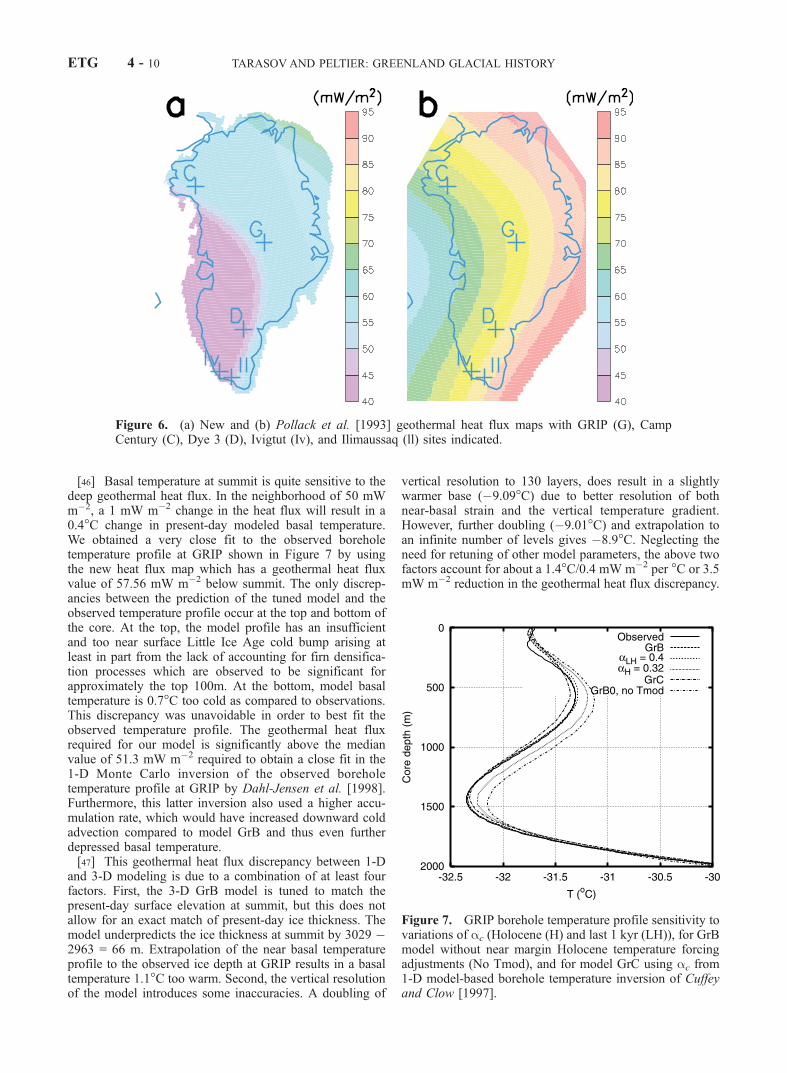
[40] The deep geothermal heat flux from the Earth intothe base of the Greenland ice sheet is largely unknown. Themost recent and thorough attempt to develop a global heatflux map is based on a mixture of direct observations andbedrock geology [Pollack et al., 1993]. According to thismodel, which is illustrated in Figure 6 for the region ofGreenland, a strong horizontal gradient should exist acrossthis region. However, the lack of local heat flow measure-ments in this region leaves the model poorly constrained.[41] Determination of background geothermal heat flux

through the inversion of observed borehole basal temper-

atures using thermomechanically coupled ice sheet (andbedrock) models offers the possibility of further constrain-ing the geothermal heat flux for ice-covered regions. Directinput of the heat flux map of Pollack et al. [1993] into ourcoupled ice sheet model was found to produce excessivelywarm basal temperatures. Given the few available con-straints, we chose to apply a series of bounded lineartransformations to this heat flux map in order that thecoupled model could be forced to approximately matchthe present-day observed basal temperatures at the threeboreholes through the ice sheet from which such data isavailable. For the sake of simplicity and also to improve thematch of the predictions of the model to RSL observations,we chose to impose much weaker gradients where therewere no borehole constraints. The resultant modified heatflux map, show in Figure 6, is of course only reasonablyconstrained in the vicinity of the three data sites, denoted D,G, and C in Figure 6 (Dye 3, GRIP, and Camp Century,respectively).[42] It is clear that borehole temperature data from Ren-

land to the east, and from sites to the north and northeastand one from near the central west margin would allow usto obtain a much more highly constrained heat flux map forGreenland. It should also be mentioned that data sites nearto, or in regions of, fast flow (e.g., Camp Century and Dye3) would have more uncertainty associated with them, bothdue to the lack of explicit ice stream mechanics in the modeland to the more poorly constrained climate forcing used todrive the model than is available from more inland sitessuch as GRIP.[43] As an independent means of assessing the quality of

the new heat flux map, it is worthwhile comparing com-puted and observed present-day surface heat fluxes. Theonly useful surface measurements available are from a

Table 3. Tuning Parameters

Parameter Main Effect

Flow enhancement parameter summit elevation and topographic fitSliding parameter summit elevation and topographic fitRegional Holocene climate forcing RSL matchRegional calving sensitivity RSL matchPrecipitation sensitivity GRIP/GISP inferred accumulation chronology bounds, Age and temperature profile at GRIPRegional precipitation sensitivity RSL match and Dye 3 ice thicknessac (glacial, Holocene, late Holocene) GRIP borehole temperature profileDeep geothermal flux GRIP borehole temperature profile and Camp Century and Dye 3 basal temperatureSouthern climate forcing gradient Dye 3 ice thickness and basal temperature

Table 4. Comparison of Model GrB and Observationsa

Obs Grid Obs GrB

Volume, 1015 m3 2.828 2.848 3.276h(summit), m 3232 3244 3245H(GRIP), m 3029 2881 2963Tb(GRIP) �C �8.50 �9.24H(Dye 3), m 2037 1859 1788Tb(Dye 3), �C �13.2 �13.3H(C. Cent.), m 1387 1291 1352Tb(C. Cent.), �C �13.0 �14.7H(NGRIP), m �3100 3019 2930Tb(NGRIP), �C ��2.5 �7.47h(NGRIP), m �3000 2974 2900

aIncluded are both direct observations (Obs) and values fromobservational data sets gridded to the model grid (Grid Obs).


series of boreholes in the Precambrian shield near thesouthern coastline of Greenland at Ivigtut and Ilimaussaq[Sass et al., 1972] denoted Iv and Il, respectively, in Figure6. The respective measured values of 43 and 36 mW m�2

are uncorrected for thermal perturbations from past icecover. For model GrB, the present-day surface heat flowsat these respective sites are 13 and 40 mW m�2, areasonably close match for Ilimaussaq but definitely notfor Ivigtut. Understanding the source of such a largedifference in modeled present-day surface heat fluxbetween two proximal sites can help elucidate the sourceof the model-observation misfit at Ivigtut. The input deepgeothermal heat flux for the two sites, 41 and 44 mW m�2,respectively, are clearly not the source of the 27 mW m�2

difference between the modeled present-day surface fluxes.As demonstrated by Tarasov and Peltier [2002], who showice thickness fields for 10 and 9 ka, both sites become ice-free at about the same time in the model (between 10 and9.5 ka). Furthermore, both sites maintain surface elevationswithin approximately 200 m of each other, at least post-LGM. Climate forcing is therefore apparently not the

source of the difference. Rather, the difference betweenthe predicted heat flows is most probably due to the factorof 2 to 6 contrast in ice velocities between the two sites andthe associated >12�C difference in basal temperature thatexisted prior to onset of the ice-free state (not shown). Thehigher ice velocity at Ilimaussaq resulted in increased heatadvection from upstream basal ice and increased deforma-tion heating. Throughout most of the glacial cycle, basal iceat Ilimaussaq was at the pressure-melting point, therebyallowing basal sliding with resultant surface velocities of up310 m yr�1 at 10 ka. Ivigtut, on the other hand, neverexperiences basal sliding in the model, and basal temper-atures were approximately �20�C at LGM and �11�C justbefore deglaciation. Near or above 0�C surface temper-atures throughout the Holocene thereby resulted in a sig-nificant negative (i.e., downward) surface heat flux duringthe mid-Holocene.[44] These differences between the model and observa-

tionally determined present-day heat flux values for the twosites suggest that there is insufficient model ice velocityaround the Ivigtut site. This is corroborated by the enhancedHolocene forcing in the whole southwest region of Green-land required to obtain a reasonable match between modeland observed RSL histories as discussed by Tarasov andPeltier [2002]. Though the forcing employed in this casehas enhanced regional Holocene warming, it is clear thatpart or all of this forcing could be making up for the lack ofexplicit ice stream mechanics in the model. Increased icevelocities could result from an increased geothermal heatflux, however model tuning favors relatively low geother-mal heat flux in the south. Though other factors likely play arole, ice thickness in the southern dome region is generallyless than observed and an increase in deep geothermal heatflux would only further exacerbate this discrepancy.[45] Partial corroboration of the northeast gradient in the

deep geothermal heat flux follows from comparison ofthe observed and model predicted surface velocity field ofthe ice sheet. In a comparison with both direct and indirectmeasurements of surface velocity, Bamber et al. [2000] findthat a 3-D thermomechanical ice sheet model, using aspatially constant geothermal heat flux, underestimatesvelocities near the northern margin and overestimatesvelocities in the southern margin. Increased geothermalfluxes would tend to increase local velocities and thereforethe spatial gradients in the geothermal heat flux mappresented herein should allow a better model match toobserved velocity fields. In fact, model GrB matches towithin one grid point, eight of the 10 direct (i.e., GPS based)surface velocity measurements listed by Bamber et al.[2000]. This has been fully discussed by Tarasov andPeltier [2002]. The two discrepant sites were situatedaround Jakobshavns Isfjord, where the very high observedvelocity gradients would be difficult to capture in a modelof only moderate spatial resolution. Given that model GrBoverestimates near margin ice thickness in the north-north-west and east-northeast [Tarasov and Peltier, 2002], it isquite possible that a much stronger northeast gradient isrequired for the areas covered by our geothermal heat fluxmap that lacked borehole constraints. However, the modelwill require better representation of fast flow processes inorder to disentangle impacts of geothermal heat flux varia-tions and ice streams.

Figure 5. Snapshots from the baseline GrB modelevolution of the Greenland surface topography with thecontemporaneous modeled ice margin shown in violet.


[46] Basal temperature at summit is quite sensitive to thedeep geothermal heat flux. In the neighborhood of 50 mWm�2, a 1 mW m�2 change in the heat flux will result in a0.4�C change in present-day modeled basal temperature.We obtained a very close fit to the observed boreholetemperature profile at GRIP shown in Figure 7 by usingthe new heat flux map which has a geothermal heat fluxvalue of 57.56 mW m�2 below summit. The only discrep-ancies between the prediction of the tuned model and theobserved temperature profile occur at the top and bottom ofthe core. At the top, the model profile has an insufficientand too near surface Little Ice Age cold bump arising atleast in part from the lack of accounting for firn densifica-tion processes which are observed to be significant forapproximately the top 100m. At the bottom, model basaltemperature is 0.7�C too cold as compared to observations.This discrepancy was unavoidable in order to best fit theobserved temperature profile. The geothermal heat fluxrequired for our model is significantly above the medianvalue of 51.3 mW m�2 required to obtain a close fit in the1-D Monte Carlo inversion of the observed boreholetemperature profile at GRIP by Dahl-Jensen et al. [1998].Furthermore, this latter inversion also used a higher accu-mulation rate, which would have increased downward coldadvection compared to model GrB and thus even furtherdepressed basal temperature.[47] This geothermal heat flux discrepancy between 1-D

and 3-D modeling is due to a combination of at least fourfactors. First, the 3-D GrB model is tuned to match thepresent-day surface elevation at summit, but this does notallow for an exact match of present-day ice thickness. Themodel underpredicts the ice thickness at summit by 3029 �2963 = 66 m. Extrapolation of the near basal temperatureprofile to the observed ice depth at GRIP results in a basaltemperature 1.1�C too warm. Second, the vertical resolutionof the model introduces some inaccuracies. A doubling of

vertical resolution to 130 layers, does result in a slightlywarmer base (�9.09�C) due to better resolution of bothnear-basal strain and the vertical temperature gradient.However, further doubling (�9.01�C) and extrapolation toan infinite number of levels gives �8.9�C. Neglecting theneed for retuning of other model parameters, the above twofactors account for about a 1.4�C/0.4 mW m�2 per �C or 3.5mW m�2 reduction in the geothermal heat flux discrepancy.

Figure 6. (a) New and (b) Pollack et al. [1993] geothermal heat flux maps with GRIP (G), CampCentury (C), Dye 3 (D), Ivigtut (Iv), and Ilimaussaq (ll) sites indicated.

Figure 7. GRIP borehole temperature profile sensitivity tovariations of ac (Holocene (H) and last 1 kyr (LH)), for GrBmodel without near margin Holocene temperature forcingadjustments (No Tmod), and for model GrC using ac from1-D model-based borehole temperature inversion of Cuffeyand Clow [1997].


[48] The remaining approximately 3 mW m�2 discrep-ancy between 1-D and 3-D models is likely due to somecombination of the lack of accounting for the impact oflongitudinal stress deviations and the limitations of 1-Dmodels. The latter must ignore horizontal heat advection,assume a poorly constrained surface elevation chronology,and also must assume negligible impact from the displace-ment of summit over the glacial cycle. As will bediscussed below, the model summit is located within thegrid cell corresponding to the present-day summit onlyduring parts of interglacials and never during glacialperiods.[49] By adjusting glacial, Holocene, and late Holocene

values of ac (see Table 1), we have obtained a closematch to the observed borehole temperature profile atGRIP, with the only discernible discrepancy near thesurface, possibly due to the lack of accounting of low-density firn layers. Also shown in Figure 7 is the resultantpresent-day borehole temperature profile for the untunedmodel GrB0 (only tuned to maximum surface elevation)and for models with modified acLH (late Holocene) andac(Holocene). It should be clear that the close fit inborehole temperature profile achieved is a nontrivial con-straint on the model.[50] We have also retuned the model to use the best fit

climatic isotopic parameters of Cuffey and Clow [1997]derived by 1-D model-based inversion of the GISPIIborehole temperature profile. Following their model tun-ing, we also added a dynamic precipitation-scale correction(applied everywhere) to ensure agreement between modeland inferred accumulation history at the GISPII site. Witha 1.5 mW m�2 reduction in the model geothermal heatflux (which gives a value of 56 mW m�2 at GRIP) and anincrease in the flow enhancement parameter from 5.1 to6.0, this new model (‘‘GrC’’) also delivers a reasonablyclose fit to the observed borehole temperature profile atGRIP as shown in Figure 7. Given the significant differ-ence in Holocene climatic isotopic parameters betweenmodel GrB and that of Cuffey and Clow [1997] (0.364 and0.25, respectively), it is therefore clear that the GRIPborehole temperature profile alone provides only a limitedconstraint on inferred climate.[51] As an independent test, it is worth examining other

borehole temperature profiles (which were not employedto tune the model). Model GrB somewhat misfits theborehole temperature profile at the GISP II site as shownin Figure 8. Whether this is a consequence of limitedmodel resolution, lack of accounting for the impact oflongitudinal stresses on ice flow, inappropriate ice rheol-ogy, insufficient surface gradient in climate, or significantdiscrepancies in the transient evolution of the ice sheetgeometry is unclear. This result clearly requires that weacknowledge the limitations of current state-of-the-art 3-Dice sheet models that rely on simplified climate forcing.The predicted borehole temperature profile for the newNGRIP site is also shown in Figure 8. In comparison tothe GRIP borehole profile, GrB NGRIP is distinguished bya 63% stronger glacial cold peak and a 30% weakerHolocene warm peak along with a 1.74�C warmer basaltemperature (�7.5�). Observationally based inferencesindicate that the base of NGRIP is near the pressuremelting point, at about �2.5�C (D. Dahl-Jensen, personal

communication, 2002) which is thus much warmer thanthe model prediction. Extrapolation of model temperatureto the NGRIP site depth of 3100 m gives a temperature of�2.5 �C for the NGRIP grid cell. Thus the discrepancy inbasal temperature is largely if not entirely due to theapproximately 170 m thinner ice in the model NGRIPgrid cell. The weaker Holocene warm peak is due to thecontinuous Holocene high surface elevation of the modelNGRIP site in contradistinction to the model GRIP sitewhich experiences a mid-Holocene elevation depression ofabout 140m. During the glacial period, model NGRIP andGRIP site elevation changes were generally quite similarand therefore the colder glacial peak in the NGRIPtemperature profile is largely if not solely due to theincreasing impact with depth of advected cold ice fromhigher elevations.

3.2. Constraints on the Eemian Evolution of theGreenland Ice Sheet

[52] Having described the model and the quality of the fitto the imposed constraints, we will next proceed to use themodel to investigate Summit migration, d18O tracer predic-tions, and the constraint on Eemian Greenland ice sheetevolution.3.2.1. Summit Migration and Ice Source Elevation[53] As 1-D inversions of both the borehole temperature

and age profiles at GRIP rely on the assumption of astationary summit, it is an important check to consider thesummit location chronology of tuned 3-D models. Asshown in Figure 9, model GrB summit position matchesthe current location only during the latter parts of intergla-cials. During glacial periods, the model summit is located aquarter to half a degree to the south and oscillates a halfdegree (single grid point distance) to the west. This singlegrid point oscillation may arise solely from the limitednumerical resolution. Marshall and Cuffey [2000] find asomewhat similar pattern of summit migration, althoughwith approximately twice the migration distance. As notedby Marshall and Cuffey [2000], such summit displacementcan explain the absence of an observed bump in isochronal

Figure 8. Borehole temperature profile comparisons forGRIP, GISP II, and NGRIP. GISP II model value has beeninterpolated to a location matching the relational positioningof the GRIP and GISP II sites.


layers (‘‘Raymond bump’’ [Raymond, 1983]) under summitwhich is expected for the case of a stationary summit [e.g.,Schott-Hvidberg et al., 1997].[54] The cyclical displacement of summit also implies

that much of the ice in the GRIP ice core did not originatefrom that location. Given the d18O to temperature depend-ence on elevation, ice source elevation needs to beexplicitly taken into account in deriving a climate forcingfrom the GRIP d18O record. We have traced ice sourceelevation back to the Eemian optimal. Furthermore, toeliminate the influence of the assumption that the ice wassourced from the time-dependent elevation of the GRIPsite, we have twice iterated model runs with ice sourceelevation chronologies from previous runs (we employedthe ratio of the source elevation minus GRIP elevation to

the difference between the contemporaneous summit ele-vation and the GRIP elevation to fix the source elevationhistory for the next iteration). From approximately 70 kauntil present, ice originated from very close to the GRIPsite as shown in Figure 10. Further back in time, sourceelevation varies away from that of the contemporaneousGRIP site, bounded of course by the elevation of summitand of the GRIP site (though numerical dissipation in thetracer model occasionally oversteps these bounds). Thedifference in elevation between summit and the GRIP siteremains small until the Eemian. Most important for con-straining the Eemian minimum of the Greenland ice mass,source elevation during the Eemian minimum is effectivelythat of GRIP which is significantly below the contempo-raneous modeled summit. This will have a significantimpact on the magnitude of the contribution inferred forthe Greenland ice sheet to the Eemian sea level highstand(see below).3.2.2. D

18O Tracer Analyses[55] It has remained somewhat contentious concerning

the extent to which the Eemian section of the GRIP icecore has suffered flow/fabric disturbances and thereforedisturbances to the inferred d18O chronologies [Johnsen etal., 1997]. The profiles of certain chemical tracers acrossthe sudden apparent cooling events of the Eemian aredifficult to explain if these events were the result ofstratigraphic disturbances [Steffensen et al., 1997]. Recordsfrom the subpolar North Atlantic suggest that coupledsurface-deepwater oscillations occurred just prior to theEemian interglacial [Oppo et al., 2001]. There is also somefar-field evidence from Lake Baikal biogenic silica andmicrofossil abundance records for a mid-Eemian coolingevent [Karabanov et al., 2000]. On the other hand, themethane variations across the Eemian segment of theGRIP and GISPII cores has no counterpart in the Vostokrecord, suggesting that there is stratigraphic disturbance[Chappellaz et al., 1997]. On the basis of the apparentlymuch more stable Eemian Antarctic climate, Cuffey and

Figure 9. Greenland summit location chronology fordifferent values of the Eemian isotopic sensitivity (ac) andfor the model without regional Holocene temperatureforcing modifications (no Tmod).

Figure 10. Surface elevation chronology of contempora-neous regional summit, GRIP, and GRIP site ice source.


Marshall [2000] argue that the Vostok Deuterium recordprovides a more realistic chronology for the period prior to100 ka. We have followed their suggestion in splicing theVostok chronology onto the Greenland record with extremalamplitude adjusted to that of the GRIP record. However,this is problematic in that matching of the extremalamplitude from the last 250 kyr (see the reconstructionlabeled DVw in Figure 11) results in a significantly differentreconstruction as opposed to matching for the period priorto 105 ka (reconstruction DV). Unless otherwise specified,we will therefore use the DV chronology for subsequentanalyses.[56] The synthetic GRIP d18O profiles obtained in this

way have an excellent match with observations for theglacial period back to just prior to the Eemian as isevident in Figure 12, further validating the quality of thetuned model. However, during the Eemian and also forthe period after last glacial maximum, phase differencesindicate limitations in the model ice sheet chronology. Forthis latter period, downward displacement of the phaseprofile indicates excessive ice accumulation at the start ofthe Holocene period. This is likely a result of thecomputationally convenient assumption of thermodynamiccontrol on temporal precipitation change which holdsreasonably well for glacial periods. This assumption hasbeen shown not to hold for the early Holocene for whichchanges in atmospheric circulation appear to dominatetemporal changes in precipitation [Cuffey and Clow,1997]. For the mid-Eemian period, the phase error ofthe model d18O profile is opposite to that of the earlyHolocene (Figure 12). This is again likely due to theimpact of atmospheric circulation changes on the regionalaccumulation rate. However, at this depth, we cannot rule

out that some phase error may also be arising fromlimitations of the ice flow chronology, possibly due tothe lack of accounting for longitudinal stresses or differ-ences in the evolved geometry of the ice sheet.[57] The impact of the assumed d18O lapse rate on the

inferred time series of surface d18O variations that isrequired to drive the tracer model is small relative to othersources of uncertainty and tends to consist of a slight shift tohigher values of the downcore d18O values relative to thosepredicted without adjustment of the lapse rate effect. It mustbe remembered that the source elevations employed for thed18O inversion are obtained by iterated tracing of ice sourcelocation for the model GRIP core. The impact of theassumed d18O lapse rate on sites further from summit willlikely be larger.

Figure 11. Modified d18O input chronologies. ChronologyDV uses the Vostok deuterium chronology for the periodprior to 105 ka with amplitude and mean adjusted so thatextremal d18O values for that period match those of the rawGRIP record. DVw is similar, except that the extremalmatch is over the whole length of the GRIP recorded. Thed18O(GRIP) is from World Data Center A for Paleoclima-tology [1997].

Figure 12. Observed and model d18O profiles at GRIPsite. Model profiles based on d18O forcings using both theraw d18O GRIP chronology and the DV (refer to text) d18Ochronology based on the Vostok Deuterium excesschronology for pre-105 ka. Also shown are results ford18O forcing without the d18O lapse rate.


[58] Validation of the tuned coupled model and of thetracer module allows a clear test of a possible source of thehigh Eemian variability of the GRIP d18O record. Compar-ison of the Eemian profiles for models driven with the rawGRIP d18O chronology and the DV d18O chronology withmuch lower Eemian variability in Figure 12 shows that withan isotropic flow law model that ignores longitudinalstresses, there is no discernible contribution to d18O Eemianvariability arising from model summit migration. Therefore,it is likely that the main source of flow disturbance to theEemian segment of the GRIP d18O record is due to dynam-ically induced folding of the stratigraphy arising fromanisotropic components of the ice rheology [Dahl-Jensenet al., 1997].[59] We have also examined whether the d18O record

could be used to constrain the Eemian d18O sensitivity totemperature and thereby indirectly Eemian extent. However,we find no significant difference in the GRIP site d18Otracer record for models using 0.312 and 0.5 values of ac forthe Eemian period.[60] While the tracer d18O profile for the GRIP site has

significant phase errors only during the interglacial andterminal glacial periods, the tracer profile for the GISP IIsite (Figure 13) displays excessive downward phase dis-placement throughout the core. The GISPII record is indeeddisplaced downward during the glacial period relative to theGRIP core, but not as much as the tracer model predicts.The tracer d18O chronologies for the GRIP and GISPII sitesare very similar and the GISPII site tracer is closer to theinferred GRIP record than to the inferred GISPII record (notshown), indicating the spatial persistence of the forcingchronology when using such a simple d18O forcing for theice sheet.[61] The d18O tracer chronology for the NGRIP site is

displaced upward by about 2.1 per mil relative to that forthe GRIP site (Figure 14). This is a direct result of the344 m difference in present-day surface elevation betweenthe two model sites and the d18O lapse rate used tocompute the upper boundary condition for the tracer.Aside from this bias, the d18O tracer for NGRIP closelyfollows the GRIP record with a cold (increasing isotopicdepletion) drift toward the Eemian arising from the nearerto summit sourcing of the older (i.e., deeper) ice. It isalso worth noting the significantly reduced signal dissi-pation at the NGRIP site that most likely arises from alonger projected horizontal relative wavelength due to astronger and more horizontal flow. Further improvementsin signal quality will likely arise further downstream untilthe vertical component of the ice flow starts to increasenear the margins. This would benefit possible futurestudies combining advanced d18O deposition models withcoupled ice sheet tracer models. Comparison of modeland far from summit ice core d18O profiles could offerpowerful constraints on the transient history of existingice sheets.3.2.3. Eemian Sea Level Contribution[62] Crucial to constraining the minimum volume of the

Greenland ice sheet during the Eemian interglacial is therepresentation of climate forcing assumed in the analysis, orin this case the d18O paleothermometric calibration. If wewere to assume that ac(Holocene) is close to ac(Eemian), thedifference in ac(Holocene) between models GrB and GrC

(both of which fit the GRIP borehole temperature andinferred age profiles) already implies significant uncer-tainty in the inferred Eemian climate. Furthermore, a morecomplete probe of parameter space would likely offer aneven larger range in possible values of ac(Holocene).Other independent constraints on ac would therefore beuseful.[63] A number of processes are likely involved in

determining the value of ac [Cuffey, 2000]. One-dimen-sional model-based analyses, for instance, suggest thatchanges in source temperature and regional evaporativerecharge rates can alone explain the difference betweenobserved spatial gradients of d18O (with respect to tem-perature) and inferred temporal gradients for the Antarctic[Hendricks et al., 2000]. A different physical basis for thesmall value of acG (during the glacial period) in compar-ison to the present-day value inferred on the basis of

Figure 13. Observed and model d18O profiles at the GISPII and GRIP site using the raw GRIP d18O forcing with d18Olapse rate.


observed spatial and temporal isotopic gradients has beensuggested by AGCM-based analyses [Fawcett et al., 1997;Krinner et al., 1997; Werner et al., 2000]. A reduction in ac

from the warm Holocene to the cold glacial is attributed tothe increased seasonality of precipitation during glacialperiods with little accompanying change in the temporalform of the seasonal cycle of either the surface temper-ature or d18O. The d18O record thus becomes a morewarm-biased temperature proxy during glacial times. Otherpossible contributing factors, such as changes in the originof precipitation and changes in tropical sea surface temper-atures, have been found to be much less important inAGCM studies [Werner et al., 2000]. While an increase inpresent-day mean temperature could further reduce theseasonality of precipitation, the rate at which this takesplace as a function of temperature change is likely to bemuch less than for colder climates. For glacial climate,GCM simulations indicate a much more zonal wintercirculation which drastically reduces the transport ofmoisture to the ice sheet [Werner et al., 2000]. There isno direct evidence nor any apparent physical basis forsuggesting a similar change in atmospheric circulationwith warmer climates typical of the mid-Holocene orEemian. The impact of changes to ocean water d18O willalso be much smaller for warmer than present as comparedto colder than present climates. In contradiction therefore

to recent 1-D model-based borehole temperature inversionsfor the Holocene period, one would expect ac for periodswarmer than present to be no smaller than that for present-day and to also be larger than acG. Therefore, we base ourupper bound for ac(Eemian) on the present-day bound forac. Shuman et al. [1998] have measured the present-day(seasonally based) value of ac to be most likely between0.4 and 0.5, with 95% confidence intervals of 0.34 to 0.68[Shuman et al., 1995]. The 1-D model-based boreholetemperature inversion of Cuffey et al. [1995] also requireda value of ac of 0.47 for the last 500 years. The older andmore poorly fitting paleothermometric calibration of John-sen et al. [1989] has an ac value of 0.6 for high d18Ovalues that characterize the Holocene. Given the ranges ofthese previous analyses, we choose a value of 0.6 as adefensible upper bound for ac(Eemian).[64] As a lower bound for plausible values of ac(Eemian),

we initially choose the value of ac(Holocene) = 0.25 fromthe analyses of Cuffey and Clow [1997]. Rerunning theconstrained model using this range of Eemian ac, we obtaina range of minimum ice volumes from 2.23 to 1.12 1015

m3 for model GrB when the Vostok DV d18O chronology isassumed. Extracting sea level contributions is further com-plicated by the 7% excess present-day ice volume in themodel. Figure 15 presents estimated eustatic sea levelcontributions reduced by the ratio of the present-day excessmodel volume (i.e., by 1/1.07).[65] On the basis of the total gas content record of the

GRIP core [Raynaud et al., 1997], Cuffey and Marshall[2000] argue that the minimum Eemian elevation of theGRIP core ice was no lower than about 2900 m. Asindicated by the boxes in Figure 15, this provides anupper bound to maximum Eemian sea level contributionsof about 4.4 m and 3.9 m, respectively, for model GrBwith accounting for GRIP ice source elevation and modelGrC (without such accounting). Lower bounds for themodels are near 2 m. Different model precipitationsensitivities to temperature change likely accounts forthe model tuned with the low value of ac(Holocene)(=0.25, GrC) also having the lowest sea level contributionfor the lower boundary value of ac(Eemian). The signifi-cantly different slope of the GrC sea level sensitivitycurve suggests even further caution in interpreting model-based constraints upon the volume of the Greenland icesheet during the Eemian interglacial.[66] One way in which we might better quantify the

impact of the entire set of constraints employed to con-struct model GrB is to compare the sea level sensitivitycurve for the untuned version of GrB (Figure 15, ‘‘untunedmodel’’, with DV d18O chronology) to that for the fullytuned model. This ‘‘untuned’’ model was only tuned toapproximate present-day ice volume and elevation atsummit (using only flow enhancement and sliding param-eters). RSL dates, present-day topography, and boreholetemperature and age profile constraints were therebyignored. This relatively unconstrained model predictsapproximately an extra 0.5 m of excess Eemian sea levelcontribution arising from the prolonged period of highclimate variability.[67] While the predicted Eemian sea level excess for

Greenland is most sensitive to the assumed value forEemian isotopic sensitivity other factors are not insignif-

Figure 14. d18O chronology for GRIP and NGRIP usingthe raw GRIP d18O forcing with d18O lapse rate.


icant. Use of the d18O chronology with high Eemianvariability (i.e., the unmodified GRIP record) for theclimate forcing results in an extra 0.6 to 0.7 m sea levelcontribution. Given its dependence upon the vagaries ofmidlatitude storm track migration, it is likely that the trueEemian Greenland climate resides somewhere betweenthe extremes represented by the GRIP and Vostok DVchronologies. The assumed source elevation of the GRIPsite ice is also important. The assumption of GRIP icesourced to the contemporaneous summit can result inmore than a meter of extra sea level contribution ascompared to the assumption of locally sourced ice andmore than 0.7 m excess relative to models that take intoaccount the actual (model) source elevation of the GRIPsite ice.[68] One additional uncertainty requires consideration. As

detailed by Tarasov and Peltier [2002], our model ofGreenland ice sheet evolution required significant modifi-cations to the near coastal Holocene temperature forcing inorder to match computed and observed relative sea levelobservations. We suspect that a significant fraction of thisextra forcing is accounting for the lack of explicit fast flowmechanics in the ice sheet model. Whatever this extraforcing represents, the apparent need for this enhancedforcing during the Holocene would suggest that the degla-ciation event predicted under the assumption of a simpleclimate forcing based upon a single proxy may well under-represent the diminution of ice volume that actuallyoccurred during the Eemian. During the Holocene minimumat 8.5 ka, differences in ice volume between the fully tunedmodel and the model lacking the modified Holoceneregional temperature forcing were 3.205 1015 � 2.925 1015 = 0.28 1015 m3. Subsequent to this, differencesdiminished. If we simply take this as an additional uncer-

tainty in our estimation of the maximal excess Eemian sealevel contribution, this adds 0.7 m of possible additional sealevel contribution.[69] Most problematic is the reliance on a single climate

proxy from the summit of Greenland to derive a climatechronology for the whole of Greenland. Recent observa-tions find anticorrelations between local climatic responsesfor the east and west coastal regions [White et al., 1997].Yet it is precisely the near-margin climate that will largelydetermine the extent of Greenland ice. The apparentabsence of deep water formation in the Labrador Seaduring the Eemian interglacial [Hillaire-Marcel et al.,2001] would have limited oceanic heat transfer to theregion, suggesting limited regional warming. On the otherhand, this situation might have been caused by a largefreshwater flux from Greenland, suggesting fast and sig-nificant deglaciation. It is therefore important to investi-gate other possible constraints on the extent of EemianGreenland deglaciation.[70] Inferences on the marginal extent of the Eemian

Greenland ice sheet might be obtained from ice coreslocated in regions that were potentially deglaciated duringthe Eemian. Considering Camp Century and Dye 3, forinstance, Camp Century retains ice even for ac(Eemian) =0.312 (Figure 16), while Dye 3 is barely covered by themargin of a residual dome for ac(Eemian) = 0.6 and isfully deglaciated with ac(Eemian) = 0.5. For all cases, thesouthern dome is cutoff from the rest of the ice sheet at thetime of minimal Eemian extent, in contrast to the Hol-ocene minimal extent at �8 kyr. In the model, the icedivide upon which Camp Century resides is much morerobust against Eemian warming than the southern domeupon which Dye 3 resides. Koerner [1989] presents someevidence for Eemian ice-free conditions at both Dye 3 andCamp Century but no definitive conclusion. If observa-tions could provide strong independent evidence for bed-rock exposure at Camp Century during the Eemian, thiswould tend to imply a very strong Eemian deglaciationand a much warmer climate. On the other hand, ouranalyses do suggest that Dye 3 was ice-free during theEemian.[71] Independent observational constraints on Eemian

climate are generally lacking. However, macrofossil analy-ses of a till-covered sequence in Washington Land, north-western Greenland [Bennike and Jepsen, 2000], suggeststhat the Eemian interglacial climate was not too differentfrom modern. Given that the regional sea level adjustedwarming during the peak of the Eemian is a significant6.8�C relative to present-day for ac(Eemian) = 0.4, this datafavors a larger value of ac(Eemian) (and therefore limitedwarming).[72] The above model results and observations suggest

that a reasonable upper bound for Eemian Greenlandeustatic sea level contribution is about 5.2 m (2900 m GRIPEemian elevation limit for model GrB, with contempora-neous ice source inversion plus 0.7 m uncertainty arisingfrom Holocene model tuning as discussed above), while alower bound is no more than 2 m. However, given thenumerous sources of uncertainty, even wider bounds arepossible. More likely values are arguably bounded byac(Eemian) = ac(Holocene) (or ac(Eemian) correspondingto 2900 m minimum GRIP site elevation, whichever con-

Figure 15. Eemian excess sea level contribution fromGreenland as a function of ac, d18O chronology, andassumed ice source location for the GRIP record. ‘‘Con-temporaneous ice source inversion’’ uses iterated runs toobtain a self-consistent source elevation for the GRIP iceused in the d18O to temperature transfer function/forcing.‘‘Contemporaneous summit’’ assumes that GRIP ice issourced from the contemporaneous summit. d18O chron-ologies are as indicated (refer to text and Figure 11 fordetails).


Figure 16. Eemian minimal extent for different contemporaneous climate forcings as well as minimalHolocene extent. Present-day observed ice margin (red) and contemporaneous modeled ice margin(violet) and Camp Century (C), Dye 3 (D) and GRIP (G) sites are also shown.


straint is stronger) and by the present-day observed value ofac of approximately 0.5. This corresponds to a range ofabout 2.7 m to 4.5 m for the set of models GrB and GrC(with 0.6 extra meters added to GrC to allow for sourceelevation discrepancies and regional variations in climate).This contrasts with the 4 to 5.5 m likely range estimate ofCuffey and Marshall [2000], who use a stricter upper boundfor ac(Eemian) of 0.43 based on central Greenland boreholetemperature analyses from the last 5 kyr and who set theirlower bound to the 2900 m elevation constraint. Some ofthe range difference is also due to different model sensitiv-ities and assumed contemporaneous summit sourcing ofGRIP ice (though Cuffey has indicated that their model haslow sensitivity to assumed ice source location (K. M.Cuffey, personal communication, 2001)). For instance, atac(Eemian) = 0.36, model GrB (DV d18O chronology) hasEemian sea level contributions of 3.8 m and 4.5 m forrespectively source-traced and summit-traced ice, whileCuffey and Marshall [2000] have almost a 5 m contributionusing summit-traced ice. This increased Eemian deglacia-tion is likely due to the stronger slope-dependent feedbackin the precipitation factor that Cuffey and Marshall [2000]employed which tends to reduce summit elevation changesand thereby allow stronger inferred climate changes for agiven ac(Eemian) (refer to equation (6)). In order to matchborehole temperature and age profiles for the GRIP site, wefound it necessary to weaken the slope-dependent factor forhigher elevations (equation (5)). Given the more completeset of constraints imposed upon the model, our resultssuggest that the 5–6 m excess eustatic rise generallyassumed to characterize the penultimate interglacial [e.g.,see Rostami et al., 2000] likely also involved mass lossfrom the south polar cryosphere.

4. Conclusions

[73] In comparison to previous modeling studies of theGreenland ice sheet, we have imposed a number of newconstraints on its evolution as described herein. Precipita-tion sensitivity to climate forcing and geothermal heat fluxwere adjusted in order to obtain a close fit with the observedborehole temperature and age profile at GRIP, to provideapproximate matches to recorded basal temperature obser-vations at Dye 3 and Camp Century and to produce anaccumulation history that is bounded by inferences from theGRIP and GISP II ice cores. In so doing, we thereby alsoprovide 3-D modeling corroboration of the significantlyreduced temporal isotopic gradient (ac) relative to theobserved spatial gradient, especially for glacial climates.Obtaining model correspondence to RSL observationsrequired further regional modifications to calving andprecipitation sensitivity parameters. Further ad hoc regionalHolocene temperature forcings were also required to fit theobservations, attesting to the nontrivial nature of the com-plete set of constraints.[74] Comparisons against other ice core data allowed

independent tests of the constrained model. Limitations ofthe model were apparent in the weaker model correspond-ence to the temperature profile at the GISP II site. Thisdiscrepancy may arise from inaccuracies in the input basaland surface topographies that have been employed, fromlimitations of the shallow ice approximation in the near

summit region, from the assumption of an isotropic flowlaw [Mangeney et al., 1997], or from the simplicity of theclimate forcing. On the other hand, a close match wasachieved to the inferred GISPII borehole age profile. Futureimprovements should arise with attention to the representa-tion of firn densification and inclusion of longitudinalstresses in the flow dynamics and with the use of higher-quality data sets for present-day Greenland surface andbasal topography.[75] Our analyses have also demonstrated the utility of

semi-Lagrangian tracer methods for tracking ice age, d18O,and ice source elevation. GRIP ice has been shown to notnecessarily originate from the contemporaneous summit,even far down the core. Especially during periods ofstrong deglaciation such as near the time of minimalEemian extent, ice is sourced much more locally thanfrom the contemporaneous summit. This has a significantimpact on Eemian climate inferences from the GRIP d18Orecord.[76] Tracing d18O for different d18O forcing chronologies

has made it clear that for isotropic flow laws, summitmigration does not contribute to the strong variability ofthe Eemian segment of the GRIP d18O record. This fitslogically with the afore mentioned local sourcing of GRIPice during the Eemian. The sensitivity of downstream d18Overtical profiles to the ice flow history combined with thequality of signal preservation with high-resolution SL trac-ing offers the possibility of strong constraints on modeledice sheet evolution from far from summit ice cores.[77] Our analyses suggest that conservative bounds on

the maximum Greenland Eemian sea level contribution arein the range of 2 m to 5.2 m. Given the complexities ofnear coastal and near ice margin climate and the fact thatice sheet extent is largely governed by the climate of theseregions, we wish to emphasize that the use of a singleclimate proxy from the summit region for driving inter-glacial cycles of Greenland ice sheet models is likely themost significant uncertainty in the model-based constraintupon the volume of the Greenland ice sheet during theEemian period. Attempts to constrain the Eemian excesssea level contribution from Greenland employing model-based analyses such as our own must therefore beindulged in with caution, accepting the reality of thesignificant sources of error that we have described herein.Significant improvements to bounds on the Greenland sealevel contribution during the Eemian interglacial might beachievable with high-resolution tracer analyses for Dye 3and Camp Century ice cores in combination with a morecomplete ice sheet model (i.e., that includes firn densifi-cation, longitudinal stresses, and more accurate basal andsurface elevation data sets). Independent Eemian climateconstraints for near margin regions would also be valuablein this context.[78] A primary reason for attempting to bound the Green-

land contribution to the Eemian highstand of sea level is toconstrain the residual contribution that must be requiredfrom the potentially unstable West Antarctic ice sheet.However, asynchronicity adds another complication to thisinference of Antarctic Eemian instability [Cuffey and Mar-shall, 2000]. Given the approximately 3 kyr phase lagbetween initial Antarctic and Greenland warming afterLGM [Sowers and Bender, 1995] and the 1.5 to 3 kyr


phase lag for a number of millennial-scale warming events[Blunier and Brook, 2001], it is unlikely that both icesheets would have simultaneously reached their minimumEemian extent. As such, estimates for Antarctic minimabased on residual sea level contributions (i.e., afteraccounting for Greenland) must be interpreted as lowerlimits. Greenland extent is, furthermore, largely undermore direct climate controls impacting on margin ablation.Grounded West Antarctic ice volume is largely governedby sea level, though subject to thermomechanicallyinduced lags [Ritz et al., 2001]. This, together with thecomplicated response of northern and southern hemi-spheric climates to orbital forcing, strongly suggests atleast some lack of synchronicity. Even a 2 kyr separationin Eemian minima would translate into an extra 0.6 m ofpossible sea level contribution for the ac(Eemian) = 0.364model. A 3 kyr separation would allow more than doublethat excess. Given the uncertainties in modeling, it is clearthat definitive partitioning of the Eemian excess sea levelcontribution between the plausible northern and southernhemispheric sources will require additional observationalconstraints. It nevertheless remains conceivable that muchif not the majority of the excessive Eemian highstand ofsea level was accounted for by Greenland. This conclusionof our analyses is potentially of great importance inrelation to the issue of the possibility that Greenland isthe most likely source of the approximately 0.6 mm yr�1

contribution to the present-day rate of global sea level risethat may be required to fully explain the otherwise missingcontribution for the present-day (but century average) rateof global sea level rise [Peltier, 2001; Douglas and Peltier,2002].

[79] Acknowledgments. This paper is a contribution to the ClimateSystem History and Dynamics Collaborative Research Network that isfunded by the Natural Sciences and Engineering Research Council ofCanada and the Atmospheric Environment Service of Canada. Additionalsupport for the work has been provided by NSERC grant A9627. GRIP andGISP II Data were provided by the National Snow and Ice Data Center,University of Colorado at Boulder, and the WDC-A for Paleoclimatology,National Geophysical Data Center, Boulder, Colorado. We would also liketo thank Kurt Cuffey for his challenging expresso-fuelled review.

ReferencesBamber, J. L., R. J. Hardy, P. Huybrechts, and I. Joughin, A comparison ofbalance velocities, measured velocities and thermomechanically mod-elled velocities for the Greenland Ice Sheet, Ann. Glaciol., 30, 211–216, 2000.

Bennike, O., and H. F. Jepsen, A new interglacial sequence from Washing-ton Land, northern Greenland, Polar Res., 9, 267–270, 2000.

Bermejo, R., On the equivalence of semi-Lagrangian and particle-in-celfinite-element methods, Mon. Weather Rev., 118, 979–987, 1990.

Bermejo, R., and A. Stanforth, The conversion of semi-Lagrangian advec-tion schemes to quasi-monotone schemes, Mon. Weather Rev., 120,2622–2632, 1992.

Blunier, T., and E. J. Brook, Timing of millennial-scale climate change inAntarctica and Greenland during the last glacial period, Science, 291,109–112, 2001.

Braithwaite, R. J., Positive degree-day factors for ablation on the Greenlandice sheet studied by energy-balance modeling, J. Glaciol., 41, 153–160,1995.

Chappellaz, J., T. Blunier, and B. Malize, CH4 and18O of O2 records from

Antarctic and Greenland ice: A clue for stratigraphic disturbance in thebottom part of the Greenland Ice Core Project and Greenland Ice SheetProject 2 ice cores, J. Geophys. Res., 102, 26,547–26,557, 1997.

Cheney, W., and D. Kincaid, Numerical Mathematics and Computing, 2nded., Brooks/Cole, Pacific Grove, Calif., 1985.

Cuffey, K. M., Methodology for use of isotopic climate forcings in ice sheetmodels, Geophys. Res. Lett., 27, 3065–3068, 2000.

Cuffey, K. M., and G. D. Clow, Temperature, accumulation and ice sheetelevation in central Greenland through the last deglacial transition,J. Geophys. Res., 102, 26,383–26,396, 1997.

Cuffey, K. M., and S. J. Marshall, Substantial contribution to sea-level riseduring the last interglacial from the Greenland ice sheet, Nature, 404,591–594, 2000.

Cuffey, K. M., G. D. Clow, R. B. Alley, M. Stuiver, E. D. Waddington, andR. W. Saltus, Large Arctic temperature change at the Wisconsin-Holo-cene glacial transition, Science, 270, 455–458, 1995.

Dahl-Jensen, D., and N. S. Gundestrup, Constitutive properties of ice atDye 3, Greenland, the physical basis of ice sheet modeling, IAHS Publ.,170, 31–43, 1987.

Dahl-Jensen, D., T. Thorsteinsson, R. Alley, and H. Shoji, Flow propertiesof the ice from the Greenland Ice Core Project ice core: The reason forfolds?, J. Geophys. Res., 102, 26,831–26,840, 1997.

Dahl-Jensen, D., N. G. K. Mosegaard, G. D. C. S. J. Johnsen, A. W.Hansen, and N. Balling, Past temperatures directly from the Greenlandice sheet, Science, 282, 268–271, 1998.

Douglas, B. C., and W. R. Peltier, The puzzle of global sea-level rise, Phys.Today, 55, 35–40, 2002.

Fawcett, P. J., A. M. Agustsdottir, R. B. Alley, C. A. S. S. Funder, andL. Hansen, The Younger Dryas termination and North Atlantic DeepWater formation: Insights from climate model simulations and Greenlandice cores, Paleoceanology, 12, 23–38, 1997.

Greve, R., M. Weis, and K. Hutter, Palaeoclimatic evolution and presentconditions of the Greenland ice sheet in the vicinity of Summit: Anapproach by large-scale modelling, Palaeoclim. Data Model., 2, 133–162, 1998.

Hendricks, M. B., D. J. Depaolo, and R. C. Cohen, Space and time variationof d18O and dD in precipitation: Can paleotemperature be estimated fromice cores, Global Biogeochem. Cycle, 14, 851–861, 2000.

Hillaire-Marcel, C., A. de Vernal, G. Bilodeau, and A. J. Weaver, Absenceof deep-water formation in the Labrador Sea during the last interglacialperiod, Nature, 410, 1073–1077, 2001.

Huybrechts, P., The Antarctic ice sheet during the last glacial-interglaicalcycle: A three-dimensional experiment, Ann. Glaciol., 14, 115–119,1990.

Huybrechts, P., Formation and disintegration of the Antarctic ice sheet,Ann. Glaciol., 20, 336–340, 1994.

Huybrechts, P., A. Letreguilly, and N. Reeh, The Greenland ice sheet andgreenhouse warming, Palaeogeogr. Palaeoclimato. Palaeoecol., 89,399–412, 1991.

Janssens, I., and P. Huybrechts, The treatment of meltwater retention inmass-balance parameterizations of the Greenland ice sheet, Ann. Glaciol.,31, 2000.

Johnsen, S. J., W. Dansgaard, and J. W. C. White, The origin of Arcticprecipitation under present and glacial conditions, Tellus, 41, 452–469,1989.

Johnsen, S. J., D. Dahl-Jensen, W. Dansgaard, and N. S. Gundestrup,Greenland palaeotemperatures derived from GRIP bore hole temperatureand ice core isotope profiles, Tellus, 47B, 624–629, 1995.

Johnsen, S. J., et al., The d18O record along the Greenland Ice Core Projectdeep ice core and the problem of possible Eemian climatic instability,J. Geophys. Res., 102, 26,397–26,410, 1997.

Karabanov, E. B., A. A. Propenko, D. F. Williams, and G. K. Khursevich,Evidence for mid-Eemian cooling in continental climatic record fromLake Baikal, J. Paleolimnol., 23, 365–371, 2000.

Koerner, R. M., Ice core evidence for extensive melting of the Greenlandice sheet in the last interglacial, Science, 244, 964–967, 1989.

Krinner, G., C. Genthon, and J. Jouzel, GCM analysis of local influences onice core delta signals, Geophys. Res. Lett., 24, 2825–2828, 1997.

Legates, D. R., and C. J. Willmott, Mean seasonal and spatial variability ingauge-corrected global precipitation, Int. J. Climatol., 10, 111–127,1990.

Mangeney, A., F. Califano, and K. Hutter, A numerical study of anisotropic,low Reynolds number, free surface flow for ice sheet modeling, J. Geo-phys. Res., 102, 22,749–22,764, 1997.

Marshall, S. J., and K. M. Cuffey, Peregrinations of the Greenland ice sheetdivide in the last glacial cycle: Implications for central Greenland icecores, Earth Planet. Sci. Lett., 179, 73–90, 2000.

McCalpin, J. D., A quantitative analysis of the dissipation inherent in semi-Lagrangian advection, Mon. Weather Rev., 116, 2330–2336, 1988.

McDonald, A., Accuracy of mulitply-upstream, semi-Lagrangian advectiveschemes, Mon. Weather Rev., 112, 1267–1275, 1984.

Meese, D. A., A. J. Gow, R. B. Alley, G. A. Zielinski, P. M. Grootes,M. Ram, K. C. Taylor, P. A. Mayewski, and J. F. Bolzan, The GreenlandIce Sheet Project 2 depth-age scale: Methods and results, J. Geophys.Res., 102, 26,411–26,423, 1997.

Ohmura, A., New temperature distribution maps for Greenland,Z Gletscherkd. Glazialgeol., 23, 1–45, 1987.


Ohmura, A., and N. Reeh, New precipitation and accumulation maps forGreenland, J. Glaciol., 37, 140–148, 1991.

Ohmura, A., P. Calanca, M. Wild, and M. Anklin, Precipitation, accumula-tion and mass balance of the Greenland ice sheet, Z. Gletscherkd. Gla-zialgeol., 35, 1–20, 1991.

Oppo, D. W., L. D. Keigwin, J. F. McManus, and J. L. Cullen, Persistentsuborbital climate variability in marine isotope stage 5 and termination II,Paleoceanography, 16, 280–292, 2001.

Peltier, W. R., The impulse response of a Maxwell Earth, Rev. Geophys., 12,649–669, 1974.

Peltier, W. R., Glacial isostatic adjustment ii: The inverse problem, Geo-phys. J. R. Astron. Soc., 46, 669–706, 1976.

Peltier, W. R., Mantle viscosity and ice age ice sheet topography, Science,273, 1359–1364, 1996.

Peltier, W. R., Postglacial variations in the level of the sea: Implications forclimate dynamics and solid-earth geophysics, Rev. Geophys., 36, 603–689, 1998.

Peltier, W. R., Global glacial isostatic adjustment and modern instrumentalrecords of relative sea level history, in Sea Level Rise: History and Con-sequences, edited by B. C. Douglas, M. S. Kearney, and S. P. Leather-man, pp. 65–95, Academic, San Diego, Calif., 2001.

Peltier, W. R., and X. Jiang, Mantle viscosity from the simultaneous inver-sion of multiple data sets pertaining to postglacial rebound, Geophys.Res. Lett., 23, 503–506, 1996.

Pollack, H. N., S. J. Hurter, and J. R. Johnson, Heat flow from the Earth’sinterior: Analysis of the global data set, Rev. Geophys., 31, 267–280,1993.

Raymond, C. F., Deformation in the vicinity of ice divides, J. Glaciol., 29,357–373, 1983.

Raynaud, D., J. Chappellaz, C. Ritz, and P. Martinerie, Air content alongthe Greenland Ice Core Project core: A record of surface climatic para-meters and elevation in central Greenland, J. Geophys. Res., 102,26,607–26,613, 1997.

Reames, F. M., and T. H. Zapotocny, Inert trace constituent transport insigma and hybrid isentropic-sigma models, part ii, Twelve semi-Lagran-gian algorithms,, Mon. Weather Rev., 127, 188–200, 1999.

Ritz, C., A. Fabre, and A. Letreguilly, Sensitivity of a Greenland ice sheetmodel to ice flow and ablation parameters: Consequences for evolutionthrough the last climatic cycle, Clim. Dyn., 13, 11–24, 1997.

Ritz, C., V. Rommelaere, and C. Dumas, Modeling the evolution of Ant-arctic ice sheet over the last 420,000 years: Implications for altitudechanges in the Vostok region, J. Geophys. Res., 106, 31,943–31,964,2001.

Rostami, A., W. R. Peltier, and A. Mangini, Quaternary marine terraces, sealevel changes and uplift histoyr of Patagonia, Argentian: Comparisonswith predictions of the ICE-4G (VM2) model of the global process ofglacial isostatic adjustment, Quat. Sci. Rev., 19, 1495–1525, 2000.

Sass, J. H., B. L. Nielsen, H. A. Wollenberg, and R. J. Munroe, Heat flowand surface radioactivity at two sites in South Greenland, J. Geophys.Res., 77, 6435–6444, 1972.

Schott-Hvidberg, C., D. Dahl-Jensen, E. D. Waddington, and J. F. Bolzan,Ice flow between the Greenland Ice Core Project and Greenland Ice SheetProject 2 boreholes in central Greenland, J. Geophys. Res., 102, 26,851–26,859, 1997.

Shuman, C. A., R. B. Alley, S. Anandakrishnan, J. W. C. White, P. M.Grootes, and C. R. Stearns, Temperature and accumulation at the Green-land Summit: Comparison of high-resolution isotope profiles and satellitepassive microwave brightness temperature trends, J. Geophys. Res., 100,9165–9177, 1995.

Shuman, C. A., R. B. Alley, M. A. Fahnestock, R. A. Bindschadler, J. W. C.White, J. Winterle, and L. R. McConnell, Temperature history and accu-mulation timing for the snowpack at GISP2, central Greenland, J. Gla-ciol., 146, 21–30, 1998.

Sowers, T., and M. Bender, Climate records covering the last deglaciation,Science, 269, 210–214, 1995.

Staniforth, A., and J. Cote, Semi-Lagrangian integration schemes for atmo-spheric models—A review, Mon. Weather Rev., 119, 2206–2223, 1991.

Steffensen, J. P., H. Clausen, C. U. Hammer, M. Legrand, and M. DeAn-gelis, The chemical composition of cold events within the Eemian sectionof the Greenland Ice Core Project ice core from Summit Greenland,J. Geophys. Res., 102, 26,747–26,754, 1997.

Tarasov, L., and W. R. Peltier, Impact of thermomechanical ice sheet cou-pling on a model of the 100 kyr ice age cycle, J. Geophys. Res., 104,9517–9545, 1999.

Tarasov, L., and W. R. Peltier, Greenland glacial history and local geody-namic consequences, Geophys. J. Int., 150, 198–229, 2002.

Vezina, J., B. Jones, and D. Ford, Sea-level highstands over the last 500,000years: Evidence from the Ironshore formation on Grand Cayman BritishWest Indies, J. Sediment. Res., 69, 317–327, 1999.

Werner, M., U. Mikolajewicz, M. Himann, and G. Hoffmann, Boreholeversus iostope temperatures on Greenland: Seasonality does matter, Geo-phys. Res. Lett., 27, 723–726, 2000.

White, J. W. C., L. K. Barlow, D. Fisher, P. Grootes, J. Jouzel, S. J. Johnsen,M. Stuiver, and H. Clausen, The climate signal in the stable isotopes ofSummit, Greenland: Results of comparisons with modern climate obser-vations, J. Geophys. Res., 102, 26,425–26,439, 1997.

Williamson, D. L., and P. Rasch, Two-dimensional semi-Lagrangian trans-port with shape-preserving interpolation, Mon. Weather Rev., 117, 102–129, 1989.

World Data Center-A for Paleoclimatology, National Geophysical DataCenter, The Greenland Summit Ice Cores [CD-ROM], Boulder, Colo.,1997. (Available at http://www.ngdc.noaa.gov/paleo/icecore/greenland/summit/).

��W. R. Peltier and L. Tarasov, Department of Physics, University of

Toronto, Toronto, Ontario, Canada M5S 1A7. ( [email protected]; [email protected])


greenland glacial history, borehole constraints, and

Documents