Greedy Routing with Guaranteed Delivery

Using Ricci Flow

Jie GaoStony Brook University

Rik Sarkar, Xiaotian Yin, Feng Luo, Xianfeng David Gu

2

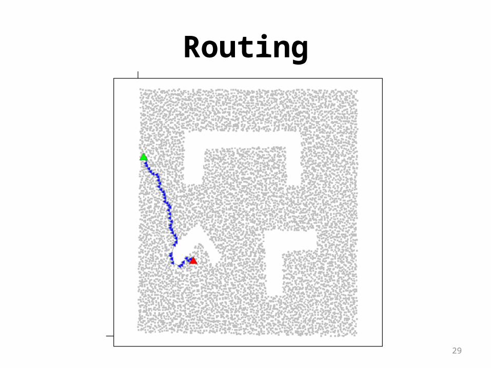
Greedy Routing• Assign coordinates to nodes • Message moves to neighbor closest to

destination• Simple, easy, compact

3

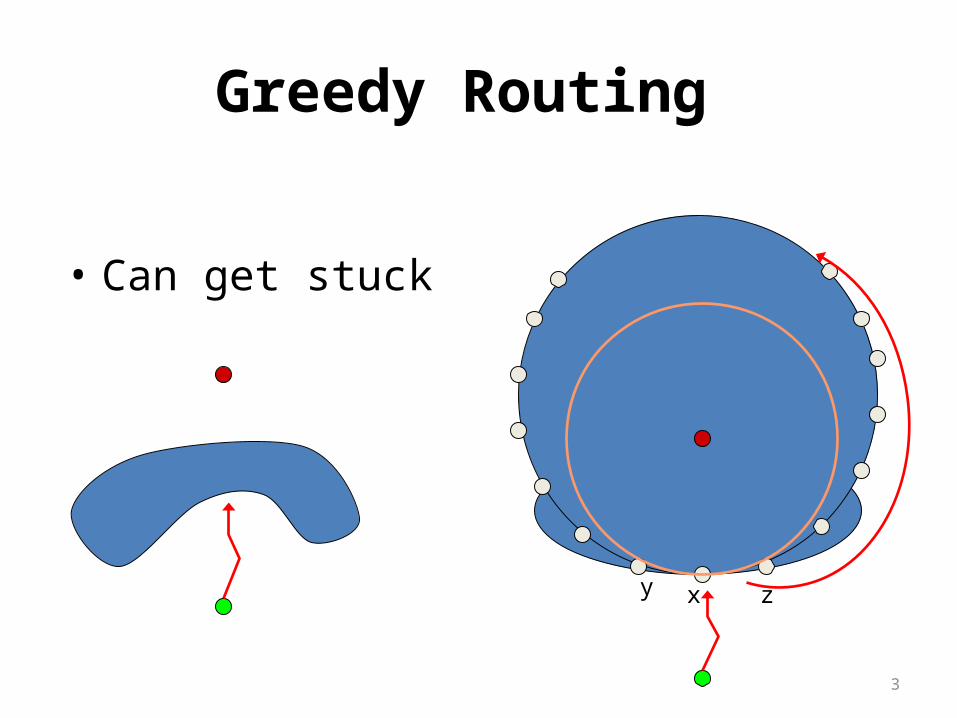
Greedy Routing

• Can get stuck

xy z

4

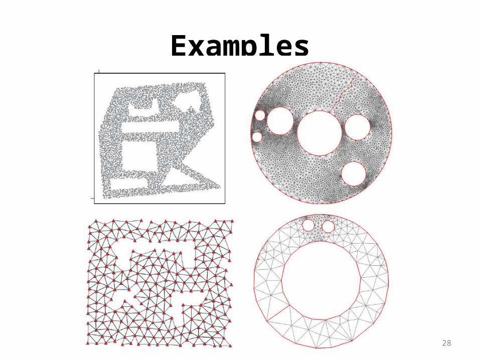
Use Ricci flow to make all holes circular

• Greedy routing does not get stuck at holes.

5

Talk Overview

• Theory on Ricci flow --smoothing out surface curvature

• Distributed algorithm on sensor network– Extract a triangulation from unit disk / quasi unit

disk graphs – Ricci flow: distributed iterative algorithm

6

Part I : Curvature and Ricci Flow

Curvature: κ = 1/RFlatter curves have smaller curvature.

R

7

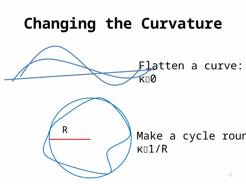
Changing the Curvature

Flatten a curve: κ0

Make a cycle roundκ1/R

R

Discrete Curvature

8

Turning angle

Sum of curvature = 2π

9

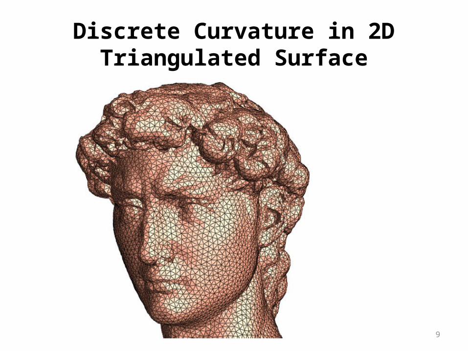
Discrete Curvature in 2D Triangulated Surface

10

Discrete Curvature in 2D Triangulated Surface

Deviation from straight line

For an interior vertex

For a vertex on the boundary

Deviation from the plane

corner angle

11

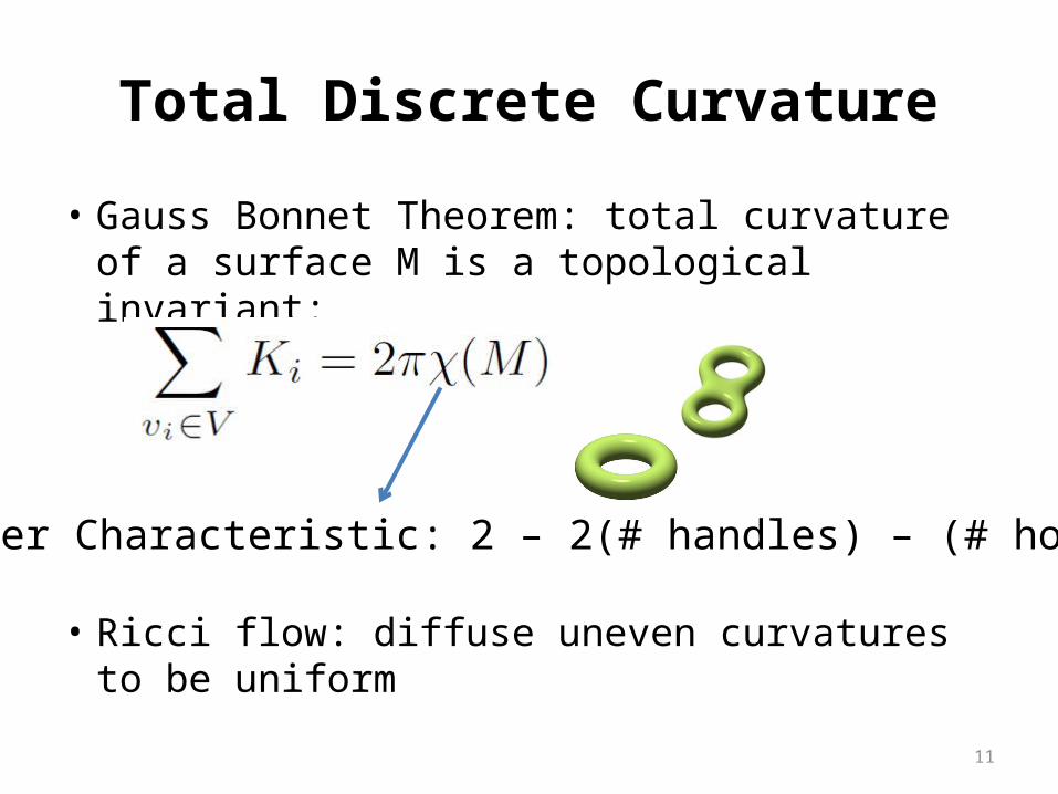
Total Discrete Curvature

• Gauss Bonnet Theorem: total curvature of a surface M is a topological invariant:

• Ricci flow: diffuse uneven curvatures to be uniform

Euler Characteristic: 2 – 2(# handles) – (# holes)

12

Sanity check: total curvature

• h holes, Euler characteristics = 2-(h+1)• Outer boundary: curvature 2π• Each inner hole: -2π• Interior vertex: 0• Total curvature: (1-h)2π

13

What they look likeNegative Curvature Positive Curvature

Ricci Flow: diffuse curvature

• Riemannian metric g on M: curve length• We modify g by curvature • Curvature evolves:

• Same equation as heat diffusion14

Δ: Laplace operator

15

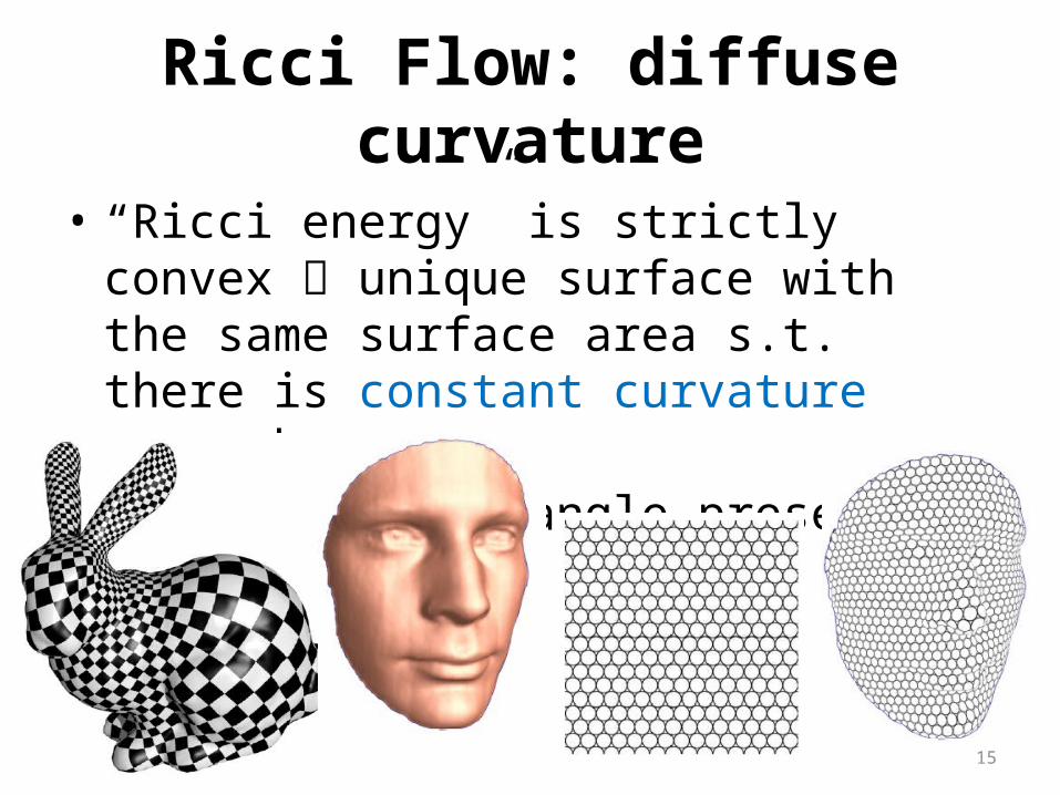
Ricci Flow: diffuse curvature

• “Ricci energy” is strictly convex unique surface with the same surface area s.t. there is constant curvature everywhere.

• Conformal map: angle preserving

16

Ricci Flow in our case

• Target: a metric with pre-specified curvature

Boundary cycle

17

Discrete Ricci Flow

• Metric: edge length of the triangulation– Satisfies triangle inequality

• Metric determines the curvature

• Discrete Ricci flow: conformal map that modifies edge length to smooth out curvature.

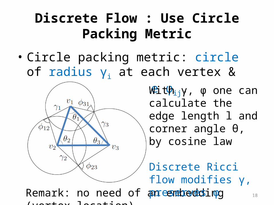
Discrete Flow : Use Circle Packing Metric

• Circle packing metric: circle of radius γi at each vertex & intersection angle φij.

Remark: no need of an embedding (vertex location) 18

With γ, φ one can calculate the edge length l and corner angle θ, by cosine law

Discrete Ricci flow modifies γ, preserves φ

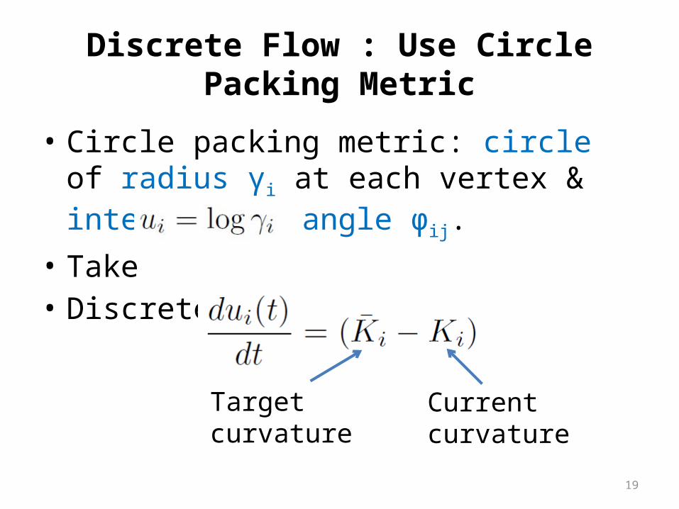
Discrete Flow : Use Circle Packing Metric

• Circle packing metric: circle of radius γi at each vertex & intersection angle φij.

• Take • Discrete Ricci flow:

19

Target curvature Current curvature

20

Background

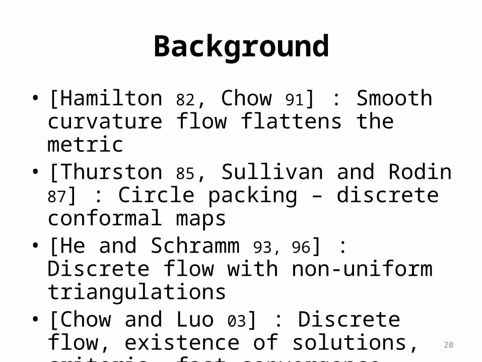
• [Hamilton 82, Chow 91] : Smooth curvature flow flattens the metric

• [Thurston 85, Sullivan and Rodin 87] : Circle packing – discrete conformal maps

• [He and Schramm 93, 96] : Discrete flow with non-uniform triangulations

• [Chow and Luo 03] : Discrete flow, existence of solutions, criteria, fast convergence

21

Part II : Ricci Flow in Sensor Networks

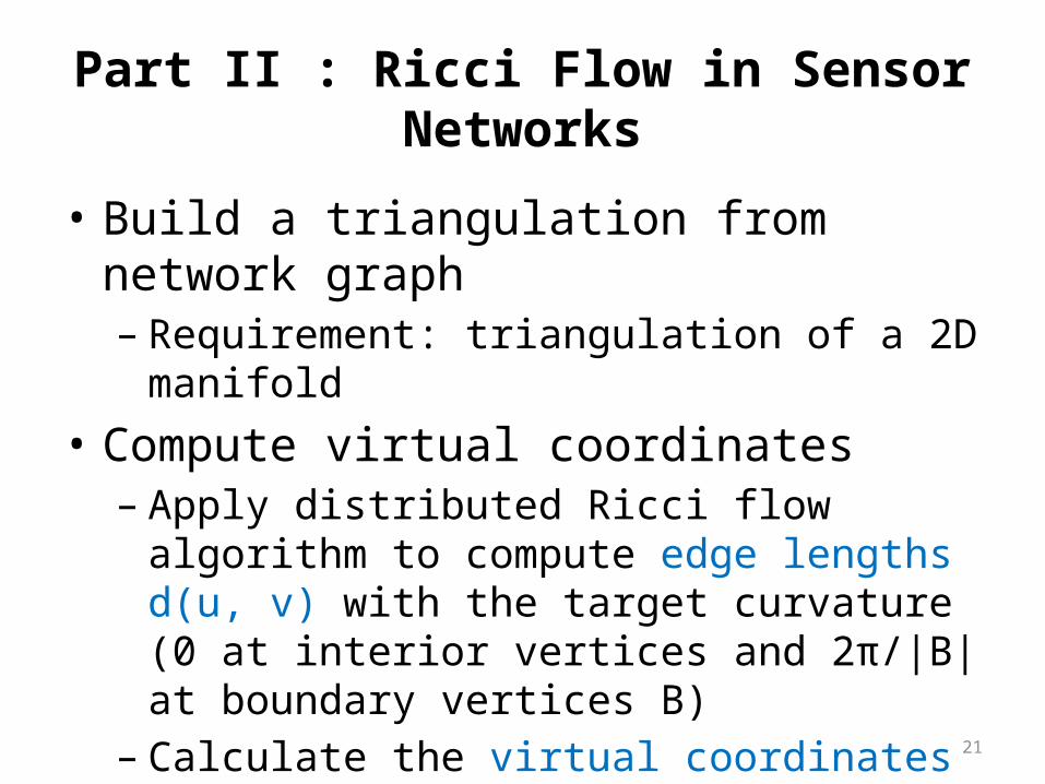
• Build a triangulation from network graph– Requirement: triangulation of a 2D manifold

• Compute virtual coordinates– Apply distributed Ricci flow algorithm to compute

edge lengths d(u, v) with the target curvature (0 at interior vertices and 2π/|B| at boundary vertices B)

– Calculate the virtual coordinates with the edge lengths d(u, v)

22

Issues with Network Graph

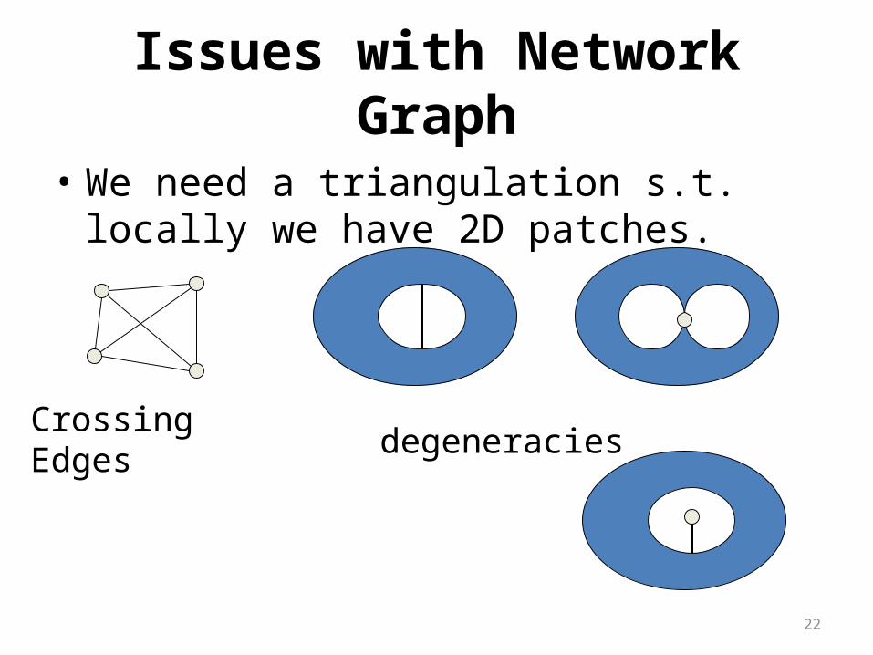
• We need a triangulation s.t. locally we have 2D patches.

Crossing Edgesdegeneracies

23

Location-based Triangulation

Local delaunay triangulations with locations[Gao, Guibas, Hershberger, Zhang, Zhu - Mobihoc 01]

• Compute Delaunay triangulations in each node’s neighborhood

• Glue neighboring local triangulations • Remove crossing edges• We now extend it to quasi-UDG

24

Location-based triangulation

• Handling Degeneracies : Insert virtual nodes

• Locations not required for Ricci flow algorithm• Set all initial edge lengths = 1

25

Location Free Triangulation• Landmark-based scheme : planar triangulation. [Funke,

Milosavljevic SODA ’07]

• Set all edge lengths = 1

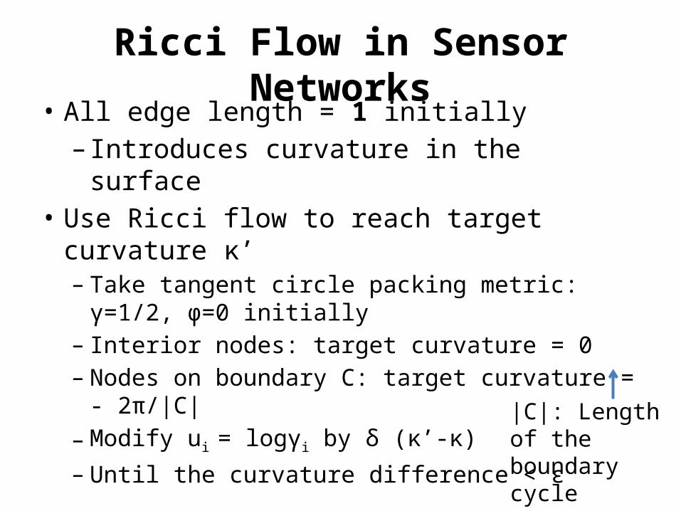
Ricci Flow in Sensor Networks• All edge length = 1 initially – Introduces curvature in the surface

• Use Ricci flow to reach target curvature κ’– Take tangent circle packing metric: γ=1/2, φ=0

initially– Interior nodes: target curvature = 0– Nodes on boundary C: target curvature = - 2π/|C|– Modify ui = logγi by δ (κ’-κ)– Until the curvature difference < ε |C|: Length of the

boundary cycle

27

Ricci Flow in Sensor Networks

• Ricci flow is a distributed algorithm– Each node modifies its own circle radius.

• Compute virtual coordinates– Start from an arbitrary triangle– Iteratively flatten the graph by triangulation.

28

Examples

29

Routing

30

Experiments and Comparison

• NoGeo : Fix locations of boundary, replace edges by tight rubber bands : Produces convex holes

[Rao, Papadimitriou, Shenker, Stoica – Mobicom 03]

• Does not guarantee delivery: cannot handle concave holes well

Method Delivery Avg Stretch

Max Stretch

Ricci Flow 100% 1.59 3.21

NoGeo 83.66% 1.17 1.54

31

Convergence rate

• Curvature error bound ε

• Step size δ• # steps =

O(log(1/ε)/δ)

Iterations Vs error

32

Theoretical guarantee of delivery

Theoretically,• Ricci flow is a numerical algorithm.• Triangles can be skinny.

• In our simulations, we have not encountered any delivery problems

• In theory, one can refine the triangulation to deal with skinny triangles

33

Summary

• Deformation of network metric by smoothing out curvatures.

• All holes are made circular.• Greedy routing always works.

• Future work: – Guarantee of stretch?– Load balancing?

35

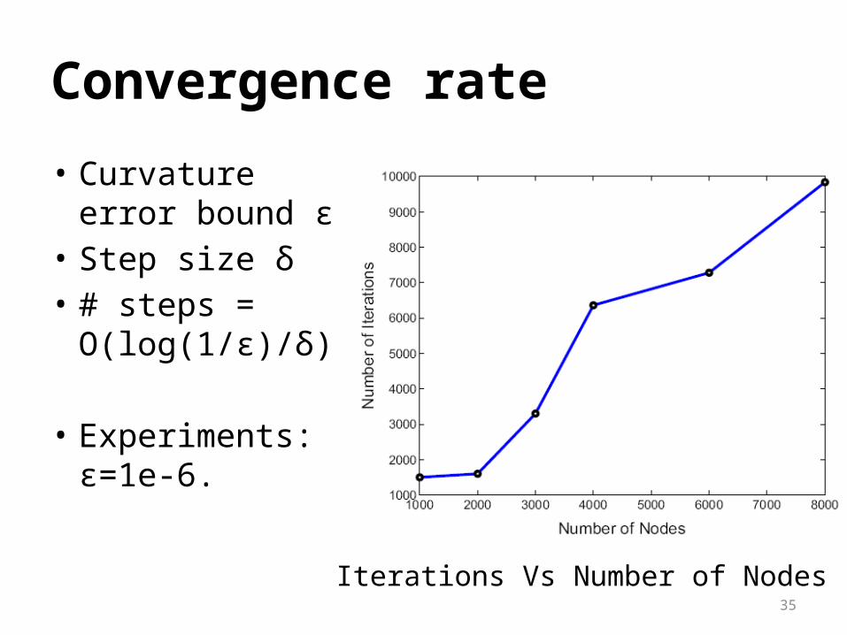
Convergence rate

• Curvature error bound ε

• Step size δ• # steps =

O(log(1/ε)/δ)

• Experiments: ε=1e-6. Iterations Vs Number of Nodes