greater sage-grouse population dynamics and probability of ...chapter fifteen greater sage-grouse...
TRANSCRIPT

CHAPTER FIFTEEN
Greater Sage-Grouse Population Dynamics and Probability of Persistence
Edward O. Garton, John W. Connelly, Jon S. Horne, Christian A. Hagen, Ann Moser, and Michael A. Schroeder
Abstract. We conducted a comprehensive analysis of Greater Sage-Grouse (Centrocercus uropha-sianus) populations throughout the species’ range by accumulating and analyzing counts of males at 9,870 leks identified since 1965. A substantial number of leks are censused each year through-out North America providing a combined total of 75,598 counts through 2007, with many leks hav-ing �30 years of information. These data sets rep-resent the only long-term database available for Greater Sage-Grouse. We conducted our analyses for 30 Greater Sage-Grouse populations and for all leks surveyed in seven Sage-Grouse Manage-ment Zones (SMZs) identified in the Greater Sage-Grouse Comprehensive Conservation Strat-egy. This approach allowed grouping of leks into biologically meaningful populations, of which 23 offered sufficient data to model annual rates of population change. The best models for describ-ing changes in growth rates of populations and SMZs, using information-theoretic criteria, were dominated by Gompertz-type models assuming density dependence on log abundance. Thirty-eight percent of the total were best described by a Gompertz model with no time lag, 32% with a one-year time lag, and 12% with a two-year time lag. These three types of Gompertz models best
portrayed a total of 82% of the populations and SMZs. A Ricker-type model assuming linear den-sity dependence on abundance in the current year was selected for 9% of the cases (SMZs or popula-tions), while an exponential growth model with no density dependence was the best model for the remaining 9% of the cases. The best model in 44% of the cases included declining carrying capacity through time of �1.8% to �11.6% per year and in 18% incorporated lower carrying capacity in the last 20 years (1987–2007) than in the first 20 years (1967–1987). We forecast future population viabil-ity across 24 populations, seven SMZs, and the range-wide metapopulation using a hierarchy of best models applied to a starting range-wide mini-mum of 88,816 male sage-grouse counted on 5,042 leks in 2007 throughout western North America. Model forecasts suggest that at least 13% of the populations but none of the SMZs may decline below effective population sizes of 50 within the next 30 years, while at least 75% of the populations and 29% of the SMZs are likely to decline below effective population sizes of 500 within 100 years if current conditions and trends persist. Preventing high probabilities of extinction in many populations and in some SMZs in the long term will require concerted efforts to decrease continuing loss and
Garton, E. O., J. W. Connelly, J. S. Horne, C. A. Hagen, A. Moser, and M. A. Schroeder. 2011. Greater Sage-Grouse population dynamics and probability of persistence. Pp. 293–381 in S. T. Knick and J. W. Connelly (editors). Greater Sage-Grouse: ecology and conservation of a landscape species and its habitats. Studies in Avian Biology (vol. 38), University of California Press, Berkeley, CA.
293
Knick_ch15.indd 293Knick_ch15.indd 293 3/1/11 11:22:10 AM3/1/11 11:22:10 AM

STUDIES IN AVIAN BIOLOGY NO. 38 Knick and Connelly294
degradation of habitat as well as addressing other factors (including West Nile virus) that may nega-tively affect Greater Sage-Grouse at local scales. Key Words: carrying capacity, Centrocercus uropha-sianus, density dependence, effective population size, Greater Sage-Grouse, lek counts, manage-ment zones, models, Ne, probability of extinction, quasi-equilibrium, time lags.
Dinámicas De Población Y Probabilidad De Persistencia Del Greater Sage-Grouse
Resumen. Condujimos un análisis comprensivo de las poblaciones del Greater Sage-Grouse (Centro-cercus urophasianus) en el rango de distribución de esta especie por medio de la acumulación y análi-sis de conteos de machos en 9,870 leks (asambleas de cortejo) identificados desde 1965. Un número considerable de leks es censado cada año en Norteamérica, lo que provee un total combinado de 75,598 conteos hasta el 2007, con muchos leks que poseen �30 años de información. Estos con-juntos de datos representan la única base de datos de largo plazo disponible para el Greater Sage-Grouse. Condujimos nuestros análisis sobre 30 poblaciones del Greater Sage-Grouse y para todos los leks examinados en siete zonas de manejo del sage-grouse (SMZs o Sage-Grouse Management Zones) que fueron identificadas en la Estrategiade Conservación Comprensiva del Greater Sage-Grouse (Greater Sage-Grouse Comprehensive Conservation Strategy). Este enfoque permitió agrupar a los leks en poblaciones biológicamente significativas de las cuales 24 ofrecieron sufi-cientes datos para modelar tasas anuales de cam-bio de la población. Los mejores modelos para describir cambios en las tasas de crecimiento de poblaciones y SMZs, usando criterios informático-teóricos, fueron dominados por modelos del tipo Gompertz asumiendo dependencia de la densidad en la abundancia del registro. El 38% del total fue mejor descrito por un modelo de Gompertz sin acción diferida del tiempo, el 32% con una acción diferida del tiempo de 1 año, y el 12% con una
acción diferida del tiempo de 2 años. Estos tres tipos de modelos Gompertz representaron mejor un total del 82% de las poblaciones y de SMZs. Un modelo de tipo Ricker asumiendo dependencia linear de densidad sobre la abundancia en el cor-riente año fue seleccionado para el 9% de los casos (SMZs o poblaciones), mientras que un modelo de crecimiento exponencial sin dependencia de den-sidad fue el mejor modelo para el restante 9% de los casos. El mejor modelo en el 44% de los casos incluyó capacidad de carga decreciente a través del tiempo de �1.8% a �11.6% por año y en el 18% incorporó capacidad de carga menor en los últi-mos 20 años (1987–2007) que en los primeros 20 años (1967–1987). Pronosticamos la viabilidad futura de la población en 24 poblaciones, siete SMZs, y la metapoblación del rango de dis-tribución utilizando una jerarquía de los mejores modelos aplicados, comenzando con un mínimo a nivel de rango de distribución de 88,816 machos de sage-grouse contados en 5,042 leks en el 2007 en Norteamérica occidental. Los pronósticos del modelo sugieren que al menos 13% de las pobla-ciones pero ninguna de las SMZs podrán dis-minuir por debajo del tamaño efectivo de la pob-lación de 50 individuos en el plazo de los próximos 30 años, mientras que es probable que el 75% de las poblaciones y 29% de las SMZs disminuyan por debajo del tamaño efectivo de la población de 500 en el plazo de 100 años si las actuales condi-ciones y tendencias persisten. Prevenir las altas probabilidades de extinción a largo plazo en muchas poblaciones y en algunas SMZs requerirá rigurosos esfuerzos para disminuir la continua pérdida y degradación del hábitat así como tam-bién atender a otros factores (incluyendo el virus del Nilo occidental) que puedan afectar negativa-mente al Greater Sage-Grouse en escalas locales. Palabras Clave: capacidad de carga, Centrocercus urophasianus, conteos de leks, cuasi-equilibrio, dependencia de la densidad, Greater Sage-Grouse, modelos, Ne, probabilidad de extinción,lapsos de tiempo, tamaño efectivo de la población, zonas de manejo.
Knick_ch15.indd 294Knick_ch15.indd 294 3/1/11 11:22:10 AM3/1/11 11:22:10 AM
GREATER SAGE-GROUSE POPULATIONS 295
Concerns about Greater Sage-Grouse (Centro-cercus urophasianus; hereafter, sage-grouse) populations have been expressed for �90
years (Hornaday 1916, Patterson 1952, Crawford and Lutz 1985, Connelly and Braun 1997). Numer-ous investigators have assessed sage-grouse popu-lation trends since the mid-1990s in various states and Canadian provinces (Braun 1995, Schroeder et al. 2000, Aldridge and Brigham 2003, Beck et al. 2003, McAdam 2003, Smith 2003). In addition, Connelly and Braun (1997) synthesized available data for nine western states and one province and concluded that sage-grouse breeding populations have declined by 17–47%. They also examined sage-grouse production data for six states (Colorado, Idaho, Montana, Oregon, Utah, and Wyoming) and reported that production declined by an over-all rate of 25%, comparing long-term averages to 1985–1994 data. Sage-grouse populations in five states were classified as secure and populations in six states and two provinces were considered at risk (Connelly and Braun 1997). More recently, changes in the range-wide distri-bution of sage-grouse were analyzed by Schroeder et al. (2004), and they concluded this species now occupies about 56% of its likely pre-European set-tlement distribution. Connelly et al. (2004) ana-lyzed lek data collected by states and provinces and concluded that sage-grouse populations declined at an overall rate of 2.0% per year from 1965 to 2003. Sage-grouse declined at an average annual rate of 3.5% from 1965 to 1985, and from 1986 to 2003 the population declined at a lower rate of 0.4% per year (Connelly et al. 2004). Recent trend analyses by the Sage- and Columbian Sharp-tailed Grouse Techni-cal Committee (Anonymous 2008) suggest a long-term decline in Greater Sage-Grouse maximum male counts, with the greatest declines from the mid-1960s to the mid-1980s. The range-wide analy-sis showed quadratic, declining trends for the 1965–2007 and 1965–1985 time frames. Connelly et al. (2004) also provided information on changes in sage-grouse populations by floristic province (Miller and Eddleman 2001). Stiver et al. (2006) suggested that sage-grouse populations should be assessed over broad scales without regard to political boundaries and indicated that floristic provinces could be slightly modified to provide Sage-Grouse Management Zones (SMZs) that would reflect ecological and biological issues and similarities. Our objectives were three-fold: (1) assess long-term changes (1965–2007) in
sage-grouse populations by SMZ (Stiver et al. 2006) and population (Connelly et al. 2004) using infor-mation obtained from lek counts, (2) use informa-tion from these lek counts to reconstruct population abundance with an index to the minimum number of males observed, and (3) evaluate the likelihood of a variety of biologically significant models and their predictions concerning long-term probability of persistence of sage-grouse populations.
METHODS
Study Area
We analyzed lek data from within the Sage-Grouse Conservation Area first delineated in Connelly et al. (2004). This area included the pre-settlement distribution of sage-grouse (Schroeder et al. 2004) buffered by 50 km. The total assessment area com-prised all or parts of 14 states and three provinces and encompassed approximately 2,063,000 km2 (Connelly et al. 2004). This area has been divided into seven SMZs that are similar to floristic regions and reflect ecological and biological similarities (Miller and Eddleman 2001). All areas occupied by sage-grouse within these floristic provinces are dominated by sage-brush (Artemisia spp.). These zones were developed by grouping sage-grouse populations within floris-tic regions (Stiver et al. 2006). Great Plains, Wyo-ming Basin, Snake River Plain, and Northern Great Basin SMZs encompassed core populations of sage-grouse (Connelly et al. 2004), while the Southern Great Basin SMZ included scattered populations in the southern part of the Great Basin. The Columbia Basin SMZ included sage-grouse in the state of Washington. The Colorado Plateau SMZ encom-passed relatively small and isolated populations in Utah and Colorado.
Population Data
Lek counts are widely used to monitor sage-grouse populations, but a report for the Western Associa-tion of Fish and Wildlife Agencies questioned their usefulness (Beck and Braun 1980). Ideally popula-tions threatened by extinction should be monitored by censusing breeding males and females and their progeny annually, yet the extensive spatial distribution of sage-grouse in regions with poor access, and the cryptic coloration and behavior of hens and their offspring preclude such an ideal
Knick_ch15.indd 295Knick_ch15.indd 295 3/1/11 11:22:10 AM3/1/11 11:22:10 AM

STUDIES IN AVIAN BIOLOGY NO. 38 Knick and Connelly296
approach. Counting breeding male sage-grouse provides a useful alternative index to the minimum number of breeding males within a local area because of their breeding behavior of concentrat-ing and displaying at open or sparsely vegetated lek sites. Further complicating the use of this index, counts over the course of a single breeding season vary from a low at the beginning of the season, to peak in the middle, followed by a decline to the end, which necessitates using the maximum count from multiple counts across the entire season as the index. Nevertheless, techniques for correctly conducting lek counts have been described (Jenni and Hartzler 1978, Emmons and Braun 1984) and problems generally seem to be related to disregard-ing accepted techniques. All lek-monitoring proce-dures are supposed to be conducted during early morning (1/2 hour before to 1 hour after sunrise) with reasonably clear and calm weather (light or no wind, partly cloudy to clear) from early March to early May (Connelly et al. 2003b). Recent and ongo-ing investigations in southern Idaho revealed that lek counts (N � 12) collected using established guidelines (Connelly et al. 2003b) based on the maximum count from �4 surveys produced a highly repeatable index with maximum and sec-ond-highest counts in a season rarely differing by �4% over multiple years (J. A. Baumgardt, unpubl. data). Timing of lek monitoring is dependent on elevation of breeding habitat and persistence of winter conditions. We examined all lek data prior to analysis to ensure they were obtained following these procedures, and in some cases we had to assume that they were collected properly. The same leks, or leks within the same area, have been counted by agency biologists for many years (Connelly et al. 2004). These leks were likely selected because they held many males, because of their accessibility, or for both reasons. Although some states and provinces attempt to monitor all known leks, leks surveyed in most states and prov-inces are not a random sample of those available, yet may provide unbiased and precise measures of the rate of change of populations when analyzed in a repeated measures framework. Connelly et al. (2004:Appendix 3) tested the lek count procedure because of potential biases in size of leks sampled and random changes in detection rates using sim-ulated populations, and reported that average annual rate of population change estimated from 20 years of data collection at 20 leks sampledper population for 10,000 simulated populations
provided unbiased estimates of the rate of change. The estimated rates of change deviated from the true simulated rate (using simulated surveys of each population) by an average of 0.04 (SD � 0.03). Precision of the estimates, measured by coefficient of determination of estimates with true simulated rates of change, increased with the simulated rate of population change from �80% for populations with an observed annual rate of change of at least 0.03 and �95% with rates of a least 0.07. Thus, while use of lek counts to assess change over a rela-tively large scale appears sound, we make no attempt to assess population dynamics at relatively small scales (e.g., harvest units, allotments) or esti-mate true population abundance using lek counts. We used three time periods for analyses. The assessment period refers to the length of time that population dynamics for a given population or SMZ is assessed; in most cases, this ranges from 1965 through 2007. An analysis period is a five-year block of time over which data are averaged and corresponds with typical planning and assess-ment periods for management agencies. The final analysis period (2000–2007) contains eight years. The previous assessment of a portion of these data indicated that populations declined more steeply during the first 20 years evaluated (1965–1985) than during the last two decades (Connelly et al. 2004). Thus, we also evaluated models incorporat-ing an early (1967–1987) and late (1987–2007) time period. We did not use the first two years of data (1965 and 1966 for most populations) to cal-culate rates of change so that models built with one- and two-year delays could be assessed in an information-theoretic framework on the basis of the same set of growth rate responses (e.g., rates calculated from 1967–2007). We define a lek, for the purposes of this chapter, as a traditional display site with two or more males that has been recorded during the assessment period or within five years of that period. Substan-tial variation may exist among agencies with regard to the definition of a lek, because little pub-lished research documents the fluidity of lek estab-lishment, formation, and extinction (Connelly et al. 2004). Although we assumed all lek data used in this analysis were obtained following established procedures (Connelly et al. 2003b), our review of state and provincial databases indicated there were some exceptions and that, in a few cases, the same lek had two or more somewhat different locations. Additionally, some agencies surveyed leks from the
Knick_ch15.indd 296Knick_ch15.indd 296 3/1/11 11:22:10 AM3/1/11 11:22:10 AM

GREATER SAGE-GROUSE POPULATIONS 297
air in addition to using ground counts. Therefore, we carefully examined each state’s and province’s database and removed questionable data, e.g., leks for which no count data could be provided, and replicate locations (�2 separate but nearby loca-tions that represented the same lek). Many states had spatial data for leks but were lacking count data associated with them and thus no way of con-firming that they actually were leks. We eliminated these data as well as leks when there was only a single count in a season for that lek and we elimi-nated data collected from the air regardless of the number of replicate counts in a year. All information relating to population dynam-ics refers to changes in breeding populations. Delineating boundaries between local concentra-tions of breeding individuals (demes), popula-tions, and metapopulations requires information on genetics, movements, habitat boundaries, and correlations in demographic rates (Garton 2002) that is sparsely available for sage-grouse across their extensive distribution (Fig. 15.1). Connelly et al. (1988) suggested that sage-grouse popula-tions be defined on a temporal and spatial basis. A breeding population can be defined as a group of sage-grouse associated with one or more
occupied leks in the same geographic area sepa-rated from other leks by �20 km (Connelly et al. 2003b). We followed these definitions for this analysis, and further defined sage-grouse popula-tions throughout their North American distri-bution based on the known locations of leks. Concentrated areas of leks were considered breed-ing populations if they were separated from the nearest adjacent concentration of leks by at least 30 km and/or separated by unsuitable habitat such as mountain ranges, desert, or large areas of cropland (Connelly et al. 2004). These were grouped into SMZs including the Great Plains, Wyoming Basin, Snake River Plain, Columbia Basin, Northern Great Basin, Southern Great Basin, and Colorado Plateau (Fig. 15.1) (Miller and Eddleman 2001, Connelly et al. 2004, Stiver et al. 2006). Although individual SMZs consisting of multiple populations could be treated as meta-populations, three factors led us to combine data for all leks within SMZs into large single popula-tions and only treat combinations of SMZs as a metapopulation: (1) our preliminary analysis indi-cated high correlations in growth rates among adjacent populations; (2) genetic studies suggest little genetic differentiation among populations
Figure 15.1. Greater Sage-Grouse populations and Sage-Grouse Management Zones in western North America.
Knick_ch15.indd 297Knick_ch15.indd 297 3/1/11 11:22:10 AM3/1/11 11:22:10 AM

STUDIES IN AVIAN BIOLOGY NO. 38 Knick and Connelly298
(Oyler-McCance and Quinn, this volume, chap-ter 5); and (3) the large sample sizes of leks in crease precision of estimates of abundance. Forty-one distinct populations have been identi-fied throughout the range of sage-grouse (Fig. 15.1) (Connelly et al. 2004). We were able to use 30 of the populations with sufficient data to allow some level of analysis (Table 15.1) and tended to include populations even if the data only included a hand-ful of leks and �10 years of successive counts. Two large populations (Great Basin core and Wyo-ming Basin) were split by SMZ boundaries, and we split each into three and two smaller popula-tions, respectively, to allow more meaningful analysis. We present findings from analyses of30 populations, seven SMZs and range-wide. We organized our findings by presenting analyses for populations within SMZs, and then the results for the SMZ. We combined all lek counts within each SMZ even if some of them came from leks within populations for which the data were too sparse to perform an individual population analy-sis. This allowed us to use all lek counts meeting our standards for quality within each SMZ. Thus, sample sizes for SMZs in a particular year are often larger than the sum of the sample sizes for populations reported within that SMZ. We con-clude with findings from a range-wide (metapop-ulation) analysis.
Monitoring Effort
We assessed monitoring effort within individual SMZs and populations by examining the average number of leks and number of active leks cen-sused over five-year periods. This allowed evalua-tion of overall monitoring effort—the number of leks counted. We calculated the change in number of leks censused to describe the manner in which monitoring effort grew exponentially over time. Methods were developed to estimate trend and annual rates of change (see below) that would not be biased by this increasing monitoring effort.
Population Trends
Lek attendance data were obtained by counting the number of males attending leks during late March and April. In some cases, counts were made over a relatively short time frame or not made in consecutive years (Aldridge and Brigham 2003). For instance, Alberta conducted lek counts
every other year for many years, while North Dakota conducted lek counts only during the third week of April, but has used this approach for �30 years. Changes in sage-grouse breeding populations can be related to changes in number of leks, changes in lek size, or both. Ability to detect changes depends on monitoring effort. Different numbers of leks were often sampled annually in all states and provinces, so total counts of males (simple sums) provide almost meaningless infor-mation (Connelly et al. 2004). We used 1965 as a baseline for descriptive statistics in most cases because monitoring efforts by agencies were most consistent thereafter, and assumed that detection rates varied stochastically among years in assess-ing population dynamics. We calculated mean lek size for all leks counted in a year based on the maximum count out of four or more counts in the year and averaged yearly means within periods to assess population change in each SMZ and population. We calculated � (annual finite rate of change) from population reconstruction and summarized it by presenting its mean and standard error for each five-year period typical of agency planning periods. We also calculated mean lek size for active leks, defined as leks counted in a year with one or more males present on any count, because if a lek moved and was not detected, or if habitat changes from fires or development ended activity at a lek, counts would continue for a limited, but variable, number of years until the lek was deleted from annual surveys (Connelly et al. 2004). We averaged these values over five-year intervals (analysis periods) to provide a broader perspective of change in sage-grouse abundance and monitoring effort.
Population Reconstruction
Sage-grouse lek counts reported by individual states and provinces were summarized within SMZs and populations, and used to reconstruct an index to the historical abundance of the popu-lation within each SMZ and population. We treated the number of males counted at leks in the final year (2007) as an index to the minimum number of males attending leks because monitor-ing effort has grown exponentially in the last 10 years. In a few regions (e.g., Washington), counting every lek was attempted in 2007, making this index equal to the minimum known number
Knick_ch15.indd 298Knick_ch15.indd 298 3/1/11 11:22:13 AM3/1/11 11:22:13 AM

TABLE 15.1Greater Sage-Grouse breeding populations in North America.
Population by management zonea Brief description of population and justification for its delineation
Great Plains SMZ I
Dakotas Small population centered in southwest North Dakota and northwest South Dakota separated from adjacent populations by �30–40 km and habitat features.
Northern Montana Large population north of Missouri River in north central Montana, southeast Alberta, and southwest Saskatchewan separated from adjacent populations by �20 km and Missouri River.
Powder River Basin, Montana Large population in southeast Montana and northeast Wyoming separated from adjacent populations by �20 km and habitat features.
Yellowstone watershed Large population in central and southeast Montana separated from adjacent populations by 20–30 km and topography.
Wyoming Basin SMZ II
Eagle–south Routt Counties, Colorado
Small population north of the Colorado River separated from adjacent populations by 20–30 km and topography.
Jackson Hole, Wyoming Small population near Jackson Hole, Wyoming, separated from adjacent populations by �50 km and topography.
Middle Park, Colorado Small population in Middle Park, Colorado, separated from adja-cent populations by 20–30 km and terrain.
Wyoming basin Large population centered in Wyoming separated from adjacent populations by 20–40 km and topography.
Southern Great Basin SMZ III
Mono Lake, California–Nevada Small population on north side of Mono Lake area in California and Nevada isolated from adjacent populations by 20–40 km and topography.
South Mono Lake, California Small population on south side of Mono Lake area in California separated from adjacent populations by 20–50 km and topography.
Northeast interior Utah Small population in northeast interior Utah separated from adjacent populations by 30–50 km and topography.
Sanpete–Emery Counties, Utah Small population in central Utah separated from adjacent populations by 50–60 km and topography.
South central Utah Small population in south central Utah separated from adjacent populations by 50–70 km and topography.
Summit–Morgan Counties, Utah Small population in northeast Utah separated from adjacent populations by 20–40 km and topography.
Tooele–Juab Counties, Utah Small population in central Utah separated from adjacent populations by 20–40 km.
Southern Great Basin A large population occupying much of central and eastern Nevada and a small portion of western Utah separated from adjacent populations by habitat and topographic features.
TABLE 15.1 (continued)
Knick_ch15.indd 299Knick_ch15.indd 299 3/1/11 11:22:14 AM3/1/11 11:22:14 AM
Population by management zonea Brief description of population and justification for its delineation
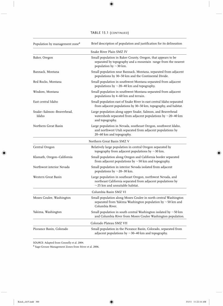
Snake River Plain SMZ IV
Baker, Oregon Small population in Baker County, Oregon, that appears to be separated by topography and a mountain range from the nearest population by �30 km.
Bannack, Montana Small population near Bannack, Montana, separated from adjacent populations by 30–50 km and the Continental Divide.
Red Rocks, Montana Small population in southwest Montana separated from adjacent populations by �20–40 km and topography.
Wisdom, Montana Small population in southwest Montana separated from adjacent populations by 4–60 km and terrain.
East central Idaho Small population east of Snake River in east central Idaho separated from adjacent populations by 30–50 km, topography, and habitat.
Snake–Salmon–Beaverhead, Idaho
Large population along upper Snake, Salmon, and Beaverhead watersheds separated from adjacent populations by �20–40 km and topography.
Northern Great Basin Large population in Nevada, southeast Oregon, southwest Idaho, and northwest Utah separated from adjacent populations by 20–60 km and topography.
Northern Great Basin SMZ V
Central Oregon Relatively large population in central Oregon separated by topography from adjacent populations by �30 km.
Klamath, Oregon–California Small population along Oregon and California border separated from adjacent populations by �50 km and topography.
Northwest interior Nevada Small population in interior Nevada isolated from adjacent populations by �20–30 km.
Western Great Basin Large population in southeast Oregon, northwest Nevada, and northeast California separated from adjacent populations by �25 km and unsuitable habitat.
Columbia Basin SMZ VI
Moses Coulee, Washington Small population along Moses Coulee in north central Washington separated from Yakima Washington population by �50 km and Columbia River.
Yakima, Washington Small population in south central Washington isolated by �50 km and Columbia River from Moses Coulee Washington population.
Colorado Plateau SMZ VII
Piceance Basin, Colorado Small population in the Piceance Basin, Colorado, separated from adjacent populations by �30–40 km and topography.
SOURCE: Adapted from Connelly et al. 2004.a Sage-Grouse Management Zones from Stiver et al. 2006.
TABLE 15.1 (CONTINUED)
Knick_ch15.indd 300Knick_ch15.indd 300 3/1/11 11:22:14 AM3/1/11 11:22:14 AM

GREATER SAGE-GROUSE POPULATIONS 301
of males attending leks. In a few populations, the largest number of leks was counted in 2005 or 2006, and that year was taken as the basis for the index to the minimum males. Lek counts in each year were considered a cluster sample of male grouse and treated by standard finite popula-tion sampling procedures for cluster samples (Scheaffer et al. 1996:297). We estimated total number of males (�) observed at all leks within a SMZ at time t as:
�(t) � n __
M (t) (Eqn. 15.1)
where an average of __
M (t) males are counted at n leks in year t. If counts were conducted at every lek within the region (e.g., Alberta and Washington), � would represent a census of all males attending leks rather than an index to the minimum number of males attending leks in year t. We estimated the precision of �(t) as:
SE � ���� n(fpc) S2M (Eqn. 15.2)
where fpc is a finite population correction which we assumed to equal 1.0 and S
M 2 is the sample
variance of males counted per lek. We assumed the finite population correction (fpc � 1.0 � pro-portion of population sampled) is equal to 1.0 because only regions where agencies attempt a complete count of leks are sampled under an approximation to true probability sampling, but even in those regions detecting new or moving leks is problematic. Thus, the true fpc is unknown, and assuming it is equal to 1.0 prevents the estimated precision of the estimators in population recon-struction from overstating their true precision. Sampling effort devoted to counting leks has varied from year to year and has grown apprecia-bly in the last 10 years. We standardized estimates and removed bias due to variable sample sizes of leks by applying a ratio estimator (Scheaffer et al. 1996) to estimate the finite rate of change (�t) for the population between successive years at leks counted in both years. Beginning with the penul-timate year (2006), males counted at each lek cen-sused in both 2006 and 2007 were treated as clus-ter samples of individual males in successive years. The ratio of males counted in a pair of suc-cessive years estimates the finite rate of change (�t) at each lek site in that one-year interval. These ratios were combined across leks within a popula-tion for each year to estimate �t for the entire population or combined across all leks within a
zone to estimate �t for that SMZ between succes-sive years as:
�(t) �
� i�1
n
Mi (t � 1)
___________
� i�1
n
Mi (t)
(Eqn. 15.3)
where Mi(t) � number of males counted at lek i in year t, across n leks counted in both years t and t � 1. Ratio estimation under classic probability sampling designs—simple random, stratified, cluster, and probability proportional to size (PPS)—assumes the sample units (leks counted in two successive years in this case) are drawn according to some random process, but the strict requirement to obtain unbiased estimates is that the ratios measured represent an unbiased sam-ple of the ratios (i.e., finite rates of change) from the population or SMZ sampled. This assump-tion seems appropriate for leks, and the possible tendency to detect larger leks than smaller leks does not bias the estimate of finite rate of change across a population or region, but makes it ana-logous to a PPS sample showing dramatically increased precision over simple random samples (Scheaffer et al. 1996). Precision (variance and standard error) of finite rates of change were esti-mated by treating �(t) as a standard ratio estima-tor (Scheaffer et al. 1996):
Var(�t) � fpc ______
n __
M (t)2
� i�1
n
[Mi(t � 1) � �(t)M(t)]2
_______________________ n � 1
(Eqn. 15.4)
where fpc is again assumed to be 1.0 to avoid over-estimating precision. An index to the relative size of the previous year population ((t)) was calculated in an analogous man-ner from the paired samples as the reciprocal of �(t):
(t) �
� i�1
n
Mi(t)
___________
� i�1
n
Mi(t � 1)
(Eqn. 15.5)
with analogous variance:
Var(t) � fpc __________
n __
M (t � 1)2
� i�1
n
[Mi(t) � tMi(t � 1)]2
______________________ n � 1
(Eqn. 15.6)
Knick_ch15.indd 301Knick_ch15.indd 301 3/1/11 11:22:14 AM3/1/11 11:22:14 AM

STUDIES IN AVIAN BIOLOGY NO. 38 Knick and Connelly302
We used these ratios to calculate an index to popula-tion size by taking the number of males counted in the final year (2007, or another base year if 2007 sample sizes of leks were inadequate) as a minimum estimate of breeding male population size within that SMZ or population. We reconstructed the previ-ous year’s minimum male abundance index by mul-tiplying the 2007 abundance by the ratio estimator of (2006), the relative number of males attending the same leks in 2006 compared to 2007. For example,�t � 0.81 between 2006 and 2007 corresponded to a (2006) of 1.23, suggesting the 15,761 males counted at 1,393 leks in 2007 were preceded by 19,461 males attending leks in 2006. This process was repeated for the change from 2005 to 2006 (�t � 1.015 indicating a (2005) of 0.985), yielding a minimum breeding male population index of 19,180 in 2005 and so on back to 1965. Repeating this process for each popula-tion and each SMZ yielded a population index for each population and zone stretching from 1965 to 2007 for populations in all SMZs except Columbia Basin and Colorado Plateau, for which valid indices were only estimable to 1967 and 1984, respectively. Application of this approach to individual popula-tions yielded reconstructed population indices for variable but generally shorter periods of time. Sam-ple sizes of leks for SMZs were much larger than the sum of leks analyzed for individual populations within each SMZ because some populations had too few leks counted over too few years to make mode-ling at the population level feasible. These small counts were feasible to include in SMZ analysesand made SMZ indices most representative of population changes within the entire zone. These population indices provided the basis for all further analyses and modeling. The variance of previous years’ population indi-ces clearly involve the variance of a product of s, with the product and therefore the variance growing progressively larger as the population reconstruc-tion is extended back further and further. We esti-mated the variance by following Goodman (1962), who proved the validity of a straightforward approach to estimating the variance of these products as:
Vâr( � i�1
k
^� i ) � �
i�1
k
(Vâr ( ^� i ) �
^� i
2 ) � � i�1
k
^� i
2 (Eqn. 15.7)
Fitting Population Growth Models
We fit a suite of stochastic population growth mod-els, including two density-independent models, to
time series of reconstructed population indices for each SMZ and population: (1) exponential growth with process error (EGPE; Dennis et al. 1991) and (2) exponential growth with differing mean ratesof change between the two time periods (period1 � 1967–1987, period 0 � 1987–2007). We also fit 24 density-dependent models consisting of all com-binations of four factors: (1) Ricker-type density dependence in population growth (Dennis and Taper 1994) or Gompertz-type density dependence in population growth (Dennis et al. 2006), (2) pres-ence or absence of a time delay in the effect density has on population growth rate (no delay, one-year delay, or two-year delay), (3) a period effect (period, as described above), and (4) time trend in popula-tion carrying capacity (year, see below). In an earlier analysis of lek data through 2003 (Connelly et al. 2004), we tested an additional model (the Gompertz state space model [GSS] Dennis et al. 2006) incor-porating observation error into the Gompertz-type density-dependent model, which consistently indi-cated that observation error in our estimates of rate of change, r(t), of populations and SMZs across large numbers of leks was close to 0. Thus, we did not include state-space models in our 26-model set. Specifically, let N(t) be the observed population index at time t, Y(t) � log[N(t)], and the annual growth rate be r(t) � Y(t � 1) � Y(t). Note that r(t) is estimated as log (�t) as described above. The global stochastic model incorporating Ricker-type density dependence was:
r(t) � a � b N(t � �) � c Year � d Period � E(t) (Eqn. 15.8)
where � � 0 for no time-delay, � � 1 for a one-year delay, or � � 2 for a two-year delay; Year is the calendar year at time t; and Period � 1 if Year � 1967–1986 and Period � 0 if Year � 1987–2007. E(t) represents environmental (i.e., process) varia-tion in realized growth rates and is a normally distributed random deviate with mean � 0 and variance � �2. The analogous model for Gompertz-type density dependence was:
r(t) � a � b ln(N(t � �)) � c Year � d Period � E(t) (Eqn. 15.9)
These models have five parameters (a, b, c, d, and �2) that can be estimated via maximum likelihood using the indices to past abundance data estimated from population reconstruction.
Knick_ch15.indd 302Knick_ch15.indd 302 3/1/11 11:22:14 AM3/1/11 11:22:14 AM

GREATER SAGE-GROUSE POPULATIONS 303
The only difference between the Ricker and Gompertz models is that Ricker assumes growth rates are a linear function of population size and Gompertz assumes growth rates are a linear function of the log of population size. Density-dependent models such as Gompertz and Ricker provide an objective approach to estimating a carrying capacity or quasi-equilibrium, which is defined as the population size at which the growth rate is 0. This quasi-equilibrium (hereafter, carry-ing capacity) represents a threshold in abundance below which population size tends to increase and above which population size tends to decrease. Several plausible scenarios for population growth can be realized from these base models. Models involving time trends (� Year) or period differences can be interpreted as inferring that carrying capacity is changing through time (e.g., negative slopes imply declines through time) or differs between time periods. For example, the parameter estimates from the Ricker model with a time trend (Year) and period effect (Period) can be used to estimate a carrying capacity as:
K � �b�1
(a � cYear � dPeriod) (Eqn. 15.10)
The hat notation over a parameter (e.g., a) indi-cates this value was the maximum likelihood esti-mate for that parameter when fit to past abun-dance data. When parameters b and c are set to 0, these models reduce to the exponential growth with process error (EGPE) model (Dennis et al. 1991). Including Period simply allows for differ-ing trends between the two time periods. We fit 26 models to each set of estimated rates of change and observed abundance index data, using the statistical computing program R Ver-sion 2.6.1 (R Development Core Team 2008) and PROC MIXED and PROC REG in SAS (SAS Institute 2006). These stochastic growth models treat annual rates of change (rt) as mixed effects of fixed effects (year and period) and random effects (reconstructed population index with or without log transformation and time lag). Annual rates of change (rt) were consistently described well by a normal distribution. We used Akaike’s information criterion corrected for small sample size (AICc) to compare the relative performance (i.e., predictive ability) of each model (Burnham and Anderson 2002). Likewise, we followed Akaike (1978, 1979, 1981, and 1983), Buckland et al. (1997) and Burnham and Anderson (2002)
in calculating Akaike weights (wi), which we treat as relative likelihoods for a model given the data:
wi � exp(�0.5 �i) ________________
� j�1
R
exp(�0.5 �j )
(Eqn. 15.11)
where �i is the difference between the AICc for model i and the lowest AICc of all R models. We report a 95% confidence set of models based on the best model using the sum of model weights �0.95 for a given analysis unit (Burnham and Anderson 2002). This approach reduces the number of mod-els reported for all analysis units to those with some potential of explaining the data but does not neces-sarily drop all models with �AICc less than 2 or 3.
Stochastic Population Projections
We performed parametric bootstraps (Efron and Tibshirani 1998) on minimum population size by projecting 100,000 replicate abundance trajecto-ries for 30 and 100 years into the future (post-2007) for each population and SMZ using:
N(t � 1) � N(t) er(t) (Eqn. 15.12)
where r(t) was the stochastic growth rate calcu-lated using maximum likelihood parameter esti-mates for the given model. For example, to project based on the Gompertz model with no time lag, a time trend in carrying capacity and a difference between periods, we used:
N(t � 1) � N(t) ea�b ln N(t) � cYear � dPeriod � E(t),
(Eqn. 15.13)
where N(0), the initial abundance for the projec-tions, was the final observed population size index (e.g., population size in 2007); Period � 0, indicat-ing that future growth would be analogous to what occurred from 1987 to 2007; and E(t) was a random deviate drawn from a normal distribution with mean 0 and standard deviation equal to � (square root of maximum likelihood estimate of mean squared error remaining from mixed model). These replicate time series were used to calculate the prob-ability that the population or SMZ would decline below a quasi-extinction threshold corresponding to minimum counts of 20 and 200 males at leks. Probability of quasi- extinction was the proportion of replications in which population abundance declined below the quasi-extinction threshold at
Knick_ch15.indd 303Knick_ch15.indd 303 3/1/11 11:22:14 AM3/1/11 11:22:14 AM

STUDIES IN AVIAN BIOLOGY NO. 38 Knick and Connelly304
some point during the time horizon (30 or 100 years). Thresholds of 20 and 200 were chosen to correspond approximately to the standard 50/500 rule for effective population sizes (Ne; Franklin 1980, Soulé 1980) expressed in terms of breeding males counted at leks and mean adult sex ratio at leks (2.5 adult females per adult male, Patterson 1952, Schroeder et al. 1999). Ne was formally defined by Sewall Wright (1938) as:
Ne � 1 ________ 1 ___ Nm
� 1 ___ Nf
(Eqn. 15.14)
where Nm � number of males successfully breed-ing and Nf � female breeders. Aldridge (2001) estimated Ne for the population of sage-grouse in Alberta (part of the northern Montana population) by applying previous esti-mates of male and female breeding success to his counts of 140 males and 280 females attending eight leks to estimate an Ne of 88. However, Bush (2009) recently used genetic tools to estimate that 46% of the males at the same leks surveyed by Aldridge successfully breed yielding Ne � 228 from Wright’s formula. This implies that Ne � 50 requires 30 males present at the lek. When Bush (2009) identified males present at the leks from individual genotypes extracted from feathers left at the lek sites during the lekking period, she found that 50% more males actually attended the site than were counted in surveys. Thus a maxi-mum count of 20 males during the lekking period is required to have 30 males present at the lek, resulting in an Ne of 50. Likewise, a minimum count of 200 males at leks in a region is required to ensure Ne � 500. In other words, forecasting future probability of a local population or SMZ declining below effective population size of 50 breeding adults (Ne � 50, corresponding to an index based on minimum males counted at leks of 20 or less) identifies populations or SMZs at short-term risk for extinction (Franklin 1980, Soulé 1980), while a local population or SMZ declining below effective population size of 500 breeding adults (Ne � 500, corresponding to an index based on minimum males counted at leks of 200 or less) identifies populations or SMZs at long-term risk for extinc-tion (Franklin 1980, Soulé 1980). Most populations and SMZs, based on our comparison of AICc values, had �1 model that could be considered a competing best model by
scoring within the 95% set. This generally meant �AICc 3. We projected future population abun-dances using each of the 26 models and used model averaging to incorporate model selection uncertainty into forecasts of population viability (Burnham and Anderson 2002) to generate an overall estimate of the probability of quasi- extinction, based on all fitted models. Generally, a model-averaged prediction can be obtained by cal-culating the predicted value of a parameter of interest (e.g., probability of quasi-extinction) for each model and taking a weighted average of the predictions where the weights are the relative likelihoods of each model:
Pr(Extinction) � � i�1
R
�Pr(Extinction�Modeliwi)
(Eqn. 15.15)
Probability of extinction under a particular model is conditional on that model and its maximum likelihood parameter estimates. We calculated a weighted variance for these probabilities of extinc-tion to assess the precision of these model- averaged probabilities of quasi-extinction (Krebs 1998) similar to the variance of a mean for grouped data (Remington and Schork 1970:46):
Var[Pr(Extinction)]
� � i�1
R
w i 2 Pr(Extinction) � Pr(Extinction�Modeli)�
2 (Eqn. 15.16)
Metapopulation Analyses
We analyzed viability of the metapopulation of sage-grouse SMZs similarly to the analysis for individual SMZs with three exceptions. First, instead of basing population projections on all 26 models, we used only the information-theoretic best models for Ricker- and Gompertz-type den-sity dependence. Second, the metapopulation model required estimated dispersal rates among SMZs. Last, correlated dynamics among SMZs were modeled by including a covariance in the random deviates used to portray environmental stochasticity. Specifically, the metapopulation was projected through time using:
NMeta(t � 1) � � j�1
7
Nj(t � 1) (Eqn. 15.17)
Knick_ch15.indd 304Knick_ch15.indd 304 3/1/11 11:22:14 AM3/1/11 11:22:14 AM

GREATER SAGE-GROUSE POPULATIONS 305
where Nj is the abundance of SMZ j. Abundance of each SMZ was projected using
Nj(t � 1) � Nj(t) e rj(t)
� � i�1�j
7
Ni(t) Dij � � i�1�j
7
Nj(t) Dji
(Eqn. 15.18)
where Dij is the dispersal rate between SMZ i and j. We followed the approach developed by Knick and Hanser (this volume, chapter 16) to estimate dispersal rates between populations within SMZs. The probability of connectivity between every pair of leks was estimated using graph theory, based on distance between known leks, the difference in size between adjacent leks, and the product of all probable steps (dispersal limited to 27 km) between the pair of leks (Knick and Hanser, this volume, chapter 16). We expressed the estimated number of probable connective links between leks in adjacent SMZs, based on graph theory, as a proportion of all the links shown between any pair of SMZs (N � 112). These proportions were standardized to an estimated maximum dispersal rate at a distance of 27 km of 0.05 (Knick and Hanser, this volume, chapter 16). The random deviate, Ej(t), for the growth rate of the jth SMZ, rj(t), was drawn from a multivariate normal distribution with mean � 0 and the sevenby seven variance/covariance matrix estimated from past abundance trajectories. We obtained estimates of covariance by correlating the residuals of the information-theoretic best models for each
SMZ pair. We used a program written in Visual Basic (MetaPVA; J. S. Horne and E. O. Garton, unpubl.) for metapopulation projections.
RESULTS
Great Plains Management Zone
This SMZ represents sage-grouse populations in parts of Alberta, Saskatchewan, Montana, North Dakota, South Dakota, and Wyoming. Most of the sage-grouse in Montana and all sage-grouse in Alberta, Saskatchewan, and the Dakotas occur in this SMZ (Fig. 15.1).
Dakotas Population
This population occupies the western portions of North and South Dakota and small parts of south-eastern Montana and northeastern Wyoming (Table 15.1). It occurs on the far eastern edge of the range of sage-grouse and is separated from other populations by distance and habitat features. The average number of leks counted per five-year period increased substantially from 1965–1969 to 2000–2007 (Table 15.2). The proportion of active leks decreased 17% over the assessment period (Table 15.2). Population trends indicated by average number of males per lek declined 46% from 1965–1969 to 1995–1999 but then recovered during 2000–2007. Average number of males per active lek demonstrated the same pattern as males/lek (Table 15.2). Average rates of change were 1.0 for three of the eight
TABLE 15.2Sage-grouse lek monitoring effort, lek size, and trends averaged over 5-yr periods for the Dakotas population, 1965–2007.
Parameter2000–2007
a1995–1999
1990–1994
1985–1989
1980–1984
1975–1979
1970–1974
1965–1969
Leks counted 56 34 37 26 27 18 19 20
Males/lek 11 7 12 11 14 10 15 13
Active leks 39 24 31 22 24 16 16 17
% active leks 69 72 84 85 92 87 89 86
Males/active lek 16 10 14 13 16 11 17 15
λ 1.004 1.148 0.913 1.013 0.965 1.116 0.883 1.128
SE (λ)b 0.091 0.108 0.060 0.077 0.099 0.155 0.078 0.114
a Eight yr of data in this period.b Standard error for annual rate of change.
Knick_ch15.indd 305Knick_ch15.indd 305 3/1/11 11:22:14 AM3/1/11 11:22:14 AM

c. Powder River Basin
b. Northern Montana
a. Dakotas
Figure 15.2. Population reconstructions for Great Plains populations and Great Plains Management Zone: (a) Dakotas; (b) northern Montana; (c) Powder River Basin; (d) Yellowstone watershed; (e) Great Plains Management Zone.
Knick_ch15.indd 306Knick_ch15.indd 306 3/1/11 11:22:15 AM3/1/11 11:22:15 AM

GREATER SAGE-GROUSE POPULATIONS 307
analysis periods. Contrary to lek size information, rate of change decreased 12.5% from the 1995–1999 analysis period to the 2000–2007 period, although both values remained at or above 1.0 for both of those periods (Table 15.2). We used our 2007 minimum population esti-mate of 939 males (SE � 120) from 120 leks to reconstruct minimum population estimates for males back to 1965 (Fig. 15.2a). The population increased from about 2,000 males in 1965 to peak above 4,000 males in 1969, followed by a continuous decline through 2007. The best stochastic model for the annual rates of change of the Dakotas population of sage-grouse was a Gompertz model with no time lags and a declining time trend of –3.2% per year (rt � 28.601 – 0.400 lnNt – 0.013 year, � � 0.2503, r2 � 0.190; Table 15.3).
The Gompertz model with declining time trend implies the Dakotas population of sage-grouse will fluctuate around carrying capacities, which will decline from 587 males attending leks in 2007 to 222 attending leks in 2037 and only 23 males in 2107 if this trend continues at the same rate in the future. The 2007 count of 939 males was 50% higher than this estimated carrying capacity. A parametric bootstrap based on the Gompertz model with declining time trend (29% relative likelihood) infers there is virtually no chance of the population declining below Ne � 50, but declining below Ne � 500 is likely (72% relative probability) within 30 years. If this trend continues for 100 years there is a 67% chance of the population declining below Ne � 50 and a 100% probability of declining below Ne � 500.
Figure 15.2. (Continued)
e. Great Plains Management Zone
d. Yellowstone watershed
Knick_ch15.indd 307Knick_ch15.indd 307 3/1/11 11:22:15 AM3/1/11 11:22:15 AM

STUDIES IN AVIAN BIOLOGY NO. 38 Knick and Connelly308
TABLE 15.3Candidate model set (contains 95% of model weight) and model statistics for
estimating population trends and persistence probabilities for Greater Sage-Grouse in the Dakotas population, 1965–2007.
Model statisticsa
Model r2 K Δ AICc wi
Gompertz � year 0.190 4 0.0b 0.288
Gompertz 0.094 3 2.0 0.106
Gompertz � year, period 0.196 5 2.3 0.092
Ricker 0.070 3 3.0 0.063
Gompertz � period 0.121 4 3.3 0.056
Ricker � year 0.119 4 3.3 0.054
EGPE 0.000 3 3.6 0.048
Gompertz t � 1 0.047 4 4.0 0.039
Gompertz t � 2 0.038 4 4.4 0.032
Gompertz t � 1 � year 0.087 5 4.8 0.026
Ricker t � 1 0.026 4 4.9 0.025
Ricker t � 2 0.022 4 5.0 0.023
Ricker � period 0.079 4 5.1 0.022
Ricker � year, period 0.132 5 5.4 0.019
Gompertz t � 2 � year 0.069 5 5.5 0.018
Period 0.009 3 5.6 0.018
Gompertz t � 1 � period 0.058 5 6.0 0.014
Gompertz t � 2 � period 0.044 5 6.6 0.011
a Model fi t described by coeffi cient of determination (r2), the number of parameters (K), the difference in Akaike’s information criterion corrected for small sample size (ΔAICc), and the AICc weights (wi).b AICc � 11.9 for best selected model.
Northern Montana Population
This population occupies parts of north-central Montana, southeast Alberta, and southwest Sas-katchewan and is separated from adjacent popula-tions by about 20 km and the Missouri River (Table 15.1). The average number of leks counted per five-year period increased substantially from 1965–1969 to 2000–2007 (Table 15.4). The proportion of active leks declined somewhat over the assessment period, but in part this may be due to the relatively few leks counted until the mid-1990s (Table 15.4). Population trends indicated by average number of males per lek declined by 61% from 1965–1969 to 1995–1999 but increased by 91% from 1995–1999 to 2000–2007. Average number
of males per active lek fluctuated but remained relatively constant over the assessment period (Table 15.4). Average rates of change were 1.0 for two of the eight analysis periods, and generally sug-gested a stable to increasing population during the 1995–1999 and 2000–2007 periods (Table 15.4). From a minimum population estimate of 3,435 males (SE � 274) in 2007 based on counts at 156 leks, we reconstructed a minimum population estimate for males from 2007 back to 1965 (Fig. 15.2b) using 1,437 lek counts reported for this period. The first population estimate of �4,700 males in 1965 was the largest for the entire time period, but it and other estimates in the late 1960s were based on only two leks counted per year, yielding standard errors as large as 15,000 males.
Knick_ch15.indd 308Knick_ch15.indd 308 3/1/11 11:22:15 AM3/1/11 11:22:15 AM

GREATER SAGE-GROUSE POPULATIONS 309
Counts of �12 leks in the mid-1970s produced more precise estimates, with standard errors declining to be no larger than the estimates by the mid-1980s. Counts of 24 to 36 leks beginning in the mid-1990s provided more precise estimates, fluctuating in the range of 3,000–3,500 males attending leks from 1995–2007 (Fig. 15.2b). The best stochastic model for the annual rates of change of the northern Montana population of sage-grouse was a Ricker model with no time lags and a period effect, suggesting that the carrying capacity in 2007 of 2,744 was 1,519 breeding males lower than in 1965–1987 (rt � 1.067 – 0.000367 Nt – 0.556 Period, � � 0. 2745, r2 � 0.357; Table 15.5). The analogous Gompertz
model had a �AICc of 1.6, an r2 of 0.331 and a relative likelihood of 22% (wi � 0.22). The Ricker model with a period effect implies the northern Montana population of sage-grouse will fluctuate around a carrying capacity of 2,908 males attending leks if the pattern of change observed in the past 20 years remains for 30 or 100 years in the future. The Gompertz model with period effect gives virtually identical predictions. A parametric bootstrap based on the Ricker model with period effect, which has a 47% relative likeli-hood, infers there is virtually no chance of the pop-ulation declining below Ne � 50 or Ne � 500 within 30 years. It is unlikely the population will decline below Ne � 50 or Ne � 500 if conditions remain
TABLE 15.4Sage-grouse lek monitoring effort, lek size, and trends averaged over 5-yr periods
for the Northern Montana population, 1965–2007.
Parameter2000–2007
a1995–1999
1990–1994
1985–1989
1980–1984
1975–1979
1970–1974
1965–1969
Leks counted 162 56 19 18 17 19 2 10
Males/lek 21 11 18 22 27 17 29 28
Active leks 123 31 15 17 16 19 2 10
% active leks 76 61 88 98 93 99 100 98
Males/active lek 28 18 20 22 28 18 29 28
λ 1.031 1.002 1.079 1.319 1.241 1.118 0.823 0.890
SE (λ)b 0.042 0.083 0.118 0.266 0.486 0.147 0.168 0.104
a Eight yr of data in this period.b Standard error for annual rate of change.
TABLE 15.5Candidate model set (contains 95% of model weight) and model statistics for
estimating population trends and persistence probabilities for greater sage-grouse in the Northern Montana population, 1965–2007.
Model statistica
Model r2 k ΔAICc wi
Ricker � period 0.357 4 0.0b 0.470
Gompertz � period 0.331 4 1.6 0.216
Ricker � year, period 0.366 5 2.0 0.171
Gompertz � year, period 0.332 5 4.1 0.060
a Model fi t described by coeffi cient of determination (r2), the number of parameters (k), the difference in Akaike’s information criterion corrected for small sample size (ΔAICc), and the AICc wt (wi).b AICc � 19.2 for best selected model.
Knick_ch15.indd 309Knick_ch15.indd 309 3/1/11 11:22:16 AM3/1/11 11:22:16 AM

TABLE 15.6Multimodel forecasts of probability (weighted mean percentage and standard error) of Greater Sage-Grouse populations
(Fig. 15.1) and Sage-Grouse Management Zones declining below Ne � 50 and Ne � 500 in 30 and in 100 yr.
Pr ( Ne) in 30 yr Pr ( Ne) in 100 yr
Populations by management zone Ne � 50 Ne � 500 Ne � 50 Ne � 500
Great Plains SMZ I�
Dakotas 4.6 39.5 44.6 66.3
Northern Montana 0.0 0.0 0.2 2.0
Powder River Basin, Montana 2.9 16.5 85.7 86.2
Yellowstone watershed 0.0 8.1 55.6 59.8
Overalla 9.5 (5.9) 11.1 (5.8) 22.8 (8.4) 24.0 (8.3)
Wyoming Basin SMZ II
Jackson Hole, Wyoming 11.2 100 27.3 100
Middle Park, Colorado 2.5 100 7.1 100
Wyoming Basin 0.0 0.0 9.9 10.7
Overalla 0.1 (0.3) 0.3 (1.1) 16.1 (7.4) 16.2 (7.4)
Southern Great Basin SMZ III
Mono Lake, California–Nevada 15.4 100.0 37.9 100.0
South Mono Lake, California 0.1 81.5 0.6 99.9
Northeast interior, Utah 0.8 51.8 8.8 78.6
Sanpete–Emery Counties, Utah 77.7 100.0 99.2 100.0
South central Utah 0.0 3.2 1.1 21.0
Summit–Morgan Counties, Utah 20.6 100.0 41.8 100.0
Tooele–Juab Counties, Utah 56.5 100.0 100.0 100.0
Southern Great Basin 0.0 2.0 4.2 78.0
Overalla 0.0 (0.0) 0.0 (0.1) 6.5 (4.9) 7.8 (5.3)
Snake River Plain SMZ IV
Baker, Oregon 61.9 100.0 66.8 100.0
Bannack, Montana 6.4 70.2 32.7 97.7
Northern Great Basin 2.1 2.5 2.5 99.7
Red Rocks, Montana 0.1 55.3 2.5 91.9
Snake–Salmon–Beaverhead, Idaho 4.2 10.2 19.3 26.8
Overalla 2.3 (1.4) 10.5 (6.1) 19.4 (7.9) 39.7 (9.6)
Northern Great Basin SMZ V
Central Oregon 4.2 15.2 74.9 91.3
Western Great Basin 5.5 6.4 6.4 99.1
Overalla 1.0 (2.0) 2.1 (2.3) 7.2 (5.0) 29.0 (8.1)
TABLE 15.6 (continued)
Knick_ch15.indd 310Knick_ch15.indd 310 3/1/11 11:22:16 AM3/1/11 11:22:16 AM

GREATER SAGE-GROUSE POPULATIONS 311
Pr ( Ne) in 30 yr Pr ( Ne) in 100 yr
Populations by management zone Ne � 50 Ne � 500 Ne � 50 Ne � 500
Columbia Basin SMZ VI
Moses Coulee, Washington 9.8 87.6 62.4 99.8
Yakima, Washington 26.1 100 50.4 100.0
Overalla 12.4 (6.0) 76.2 (6.5) 62.1 (9.1) 86.3 (5.8)
Colorado Plateau SMZ VII 0.0 (0.0) 95.6 (3.7) 5.1 (2.3) 98.4 (3.7)
Summaryb
Popns Ne � 50,500% 3 13 8 18
13% 54% 33% 75%
SMZs Ne � 50,500% 0 2 1 2
0% 29% 14% 29%
a Overall estimates (SE) are based on all leks surveyed within an SMZ including small populations not listed in table because of small sample size of leks and/or years of data collection.b Summary values are the number and percentage of populations and management zones with �50% likelihood of declining below Ne � 50 and Ne � 500.
the same for 100 years. Across all 26 models of population growth, there is only a 2% relative prob-ability of the population declining below Ne � 500 within 100 years if population changes observed in the last 43 years continue unchanged (Table 15.6).
Powder River Basin, Montana, Population
This population occupies parts of southeastern Montana and northeastern Wyoming (Table 15.1). The average number of leks counted per five-year period increased substantially from 1965–1969 to 2000–2007 (Table 15.7). The proportion of active leks declined over the assessment period (Table 15.7). Population trends, indicated by aver-age number of males per lek, declined by 45% from 1970–1974 to 2000–2007. The average number of males per active lek declined by 24% over the assessment period (Table 15.7). Average rates of change were 1.0 for three of the seven analysis periods, and decreased by 15.7% from the 1995–1999 to the 2000–2007 period, but both values remained at or above 1.0 for both periods (Table 15.7). We reconstructed a minimum population esti-mate for males from 2007 back to 1967 (Fig. 15.2c) using 2,358 lek counts reported for this period from a minimum population estimate of 5,397
males (SE � 401) in 2007, based on counts at 344 leks. The estimated population peaked at more than 76,000 males (SE � 66,799) in 1969, with irregular short-duration fluctuations or cycles (four to five years between peaks) overlaid on a strongly declining trend through 1996. Counts at leks (range � 70–350) beginning in the mid-1990s provided relatively precise estimates fluctu-ating in the range of 3,000–6,000 males attending leks from 1996 to 2007 (Fig. 15.2c). The best stochastic model for annual rates of change of the Powder River Basin population of sage-grouse was a Gompertz model with a one-year time lag and a rapidly declining time trend of �7.3% per year (rt � 60.417 – 0.377 ln(Nt�1) – 0.0286 year, � � 0.2618, r2 � 0.315), this model was supported by the data with a relative likeli-hood of 55% (Table 15.8). The Gompertz model with declining time trend implies the Powder River Basin population of sage-grouse will fluctuate around a carrying capacity that will decline from 3,042 males attending leks in 2007 to only 312 males attend-ing leks in 2037, to going extinct with only two males attending leks in 2107 if this trend contin-ues at the same rate in the future. The 2007 count of 5,397 males is estimated to be about 2,000 males higher than the carrying capacity of
TABLE 15.6 (CONTINUED)
Knick_ch15.indd 311Knick_ch15.indd 311 3/1/11 11:22:16 AM3/1/11 11:22:16 AM

STUDIES IN AVIAN BIOLOGY NO. 38 Knick and Connelly312
the region. A parametric bootstrap based on the Gompertz model with declining time trend, which has a 29% relative likelihood, infers that there is little chance (3%) of the population declining below Ne � 50 but that declining below Ne � 500 is more likely (17% relative probabil-ity) within 30 years. Multimodel projections across all 26 models forecast that if this trend
continues for 100 years there is an 86% probabil-ity of the population declining below Ne � 50 and Ne � 500 (Table 15.6).
Yellowstone Watershed Population
This population occupies much of southeastern Montana and northeastern Wyoming. It is separated
TABLE 15.7Sage-grouse lek monitoring effort, lek size, and trends averaged over 5-yr periods for the
Powder River Basin population, 1970–2007.
Parameter2000–2007
a1995–1999
1990–1994
1985–1989
1980–1984
1975–1979
1970–1974
Leks counted 239 84 66 63 62 20 14
Males/lek 12 7 12 15 22 25 22
Active leks 158 46 48 49 56 17 13
% active leks 66 54 72 78 90 81 90
Males/active lek 19 13 16 19 24 30 25
λ 1.027 1.218 0.662 1.140 0.874 1.006 0.971
SE (λ)b 0.067 0.134 0.078 0.148 0.087 0.147 0.135
a Eight yr of data in this period.b Standard error for annual rate of change.
TABLE 15.8Candidate model set (contains 95% of model weight) and model statistics for
estimating population trends and persistence probabilities for Greater Sage-Grouse in the Powder River Basin population, 1970–2007.
Model statistica
Model r2 k ΔAICc wi
Gompertz t � 1 � year 0.315 5 0.0b 0.553
Gompertz t � 1 � year, period 0.318 6 2.5 0.159
Gompertz t � 2 � year 0.242 5 3.9 0.081
Gompertz t � 1 � period 0.228 5 4.5 0.057
Gompertz t � 2 � year, period 0.249 6 6.1 0.026
Gompertz t � 2 � period 0.197 5 6.1 0.027
Ricker t � 1 � year 0.181 5 6.8 0.019
Gompertz t � 1 0.112 4 7.3 0.014
Gompertz t � 2 0.097 4 8.0 0.010
Ricker t � 1 � period 0.142 5 8.5 0.008
a Model fi t described by coeffi cient of determination (r2), the number of parameters (k), the difference in Akaike’s information criterion corrected for small sample size (ΔAICc), and the AICc wt (wi).b AICc � 15.2 for best selected model.
Knick_ch15.indd 312Knick_ch15.indd 312 3/1/11 11:22:16 AM3/1/11 11:22:16 AM

GREATER SAGE-GROUSE POPULATIONS 313
TABLE 15.9Sage-grouse lek monitoring effort, lek size, and trends averaged over 5-yr periods
for the Yellowstone watershed population, 1965–2007.
Parameter2000–2007
a1995–1999
1990–1994
1985–1989
1980–1984
1975–1979
1970–1974
1965–1969
Leks counted 346 132 133 141 130 86 53 8
Males/lek 15 12 14 15 24 22 21 17
Active leks 231 89 96 111 118 79 48 8
% active leks 68 67 74 79 91 92 89 96
Males/active lek 21 18 19 19 26 23 24 18
λ 1.009 1.170 0.911 1.092 0.914 1.053 0.974 1.247
SE (λ)b 0.052 0.084 0.061 0.068 0.050 0.071 0.104 0.191
a Eight yr of data in this period.b Standard error for annual rate of change.
from other populations by distance and topographic features (Table 15.1). The average number of leks counted per five-year period increased substantially from 1965–1969 to 2000–2007 (Table 15.9). The proportion of active leks declined over the assessment period (Table 15.9). Population trends, as indicated by average number of males per lek, declined slightly from 1965–1969 to 2000–2007. Lek size increased by �41% from 1965–1969 to 1980–1984 and then decreased by 37% from 1980–1984 to 2000–2007. Average number of males per active lek also had the same pattern over the assessment period (Table 15.9). Average rates of change were 1.0 for three of the eight analysis periods and declined by 14% between the last two analysis periods (Table 15.9). Neverthe-less, both values remained at or above 1.0 for both of the periods. From a minimum population estimate of 6,385 males (SE � 327) in 2007 based on counts at 286 leks, we reconstructed a minimum population estimate for males from 2007 back to 1966 (Fig. 15.2d) using counts at 1,169 leks reported for this period. The estimated population peaked at just below 13,000 males (SE � 940) in 1972 during a period of relative high numbers (8,000–13,000) from 1969–1984, followed by fluctuations of 3,000–9,000 until present. Counts at �100 leks beginning in 1985 provided precise minimum estimates of number of males attending leks. The best stochastic model for the annual rates of change of the Yellowstone watershed popula-tion of sage-grouse was a Ricker model with no
time lags and a declining time trend of –4.5% per year (rt � 27.938 – 0.00010421 ln(Nt) – 0.0138 year, � � 0.2204, r2 � 0.338). The analogous Gompertz model was not competitive, with only a 4% relative likelihood, while other Ricker models with Period or time � Period had high relative likelihoods (Table 15.10). The Ricker model with declining time trend implies the Yellowstone watershed population of sage-grouse will fluctuate around a carrying capacity that will decline from 2,948 males in 2007 to extinction in 2037 if this trend continues at the same rate in the future. The 2007 count was more than twice as large as the estimated carry-ing capacity. The carrying capacity in 2037 was below 0. A parametric bootstrap based on the Ricker model with declining time trend infers there is virtually no chance of the population declining below a Ne � 50, but declining below Ne � 500 is more likely (21% relative probability) within 30 years. If this trend continues for 100 years, there is a 100% probability of the popula-tion declining below Ne � 50 and Ne � 500, though multimodel forecasts across all models predict lower (56% and 60%, respectively) proba-bilities.
Comprehensive Analysis of All Leks in the Management Zone
In 1965–1969, an average of 45 leks per year was censused. By 2005–2007, an average of 830 leks per year was counted, an increase of 1,744%
Knick_ch15.indd 313Knick_ch15.indd 313 3/1/11 11:22:16 AM3/1/11 11:22:16 AM

STUDIES IN AVIAN BIOLOGY NO. 38 Knick and Connelly314
(Table 15.11). The proportion of active leks decreased over the assessment period, averaging between 90% and 92% from 1965–1984, but declining to 68% by 2005–2007 (Table 15.11). Population trends, as indicated by average number of males per lek, decreased over the assessment period by 17% while average number of males per active lek increased by 10% (Table 15.11). Average
annual rates of change were 1.0 for three of the eight analysis periods. Average annual rates of change declined by 10% from 1995–1999 to 2000–2007, but values remained at or above 1.0 for both of these periods. From a minimum population estimate of 14,814 males (SE � 609) in 2007 based on counts at 905 leks, we reconstructed a minimum
TABLE 15.10Candidate model set (contains 95% of model weight) and model statistics for
estimating population trends and persistence probabilities for Greater Sage-Grouse in theYellowstone watershed population, 1965–2007.
Model statistica
Model r2 k ΔAICc wi
Ricker � year 0.338 4 0.0b 0.385
Ricker � period 0.317 4 1.2 0.211
Ricker � year, period 0.353 5 1.8 0.160
Gompertz � year 0.279 4 3.3 0.074
Gompertz � period 0.261 4 4.3 0.045
Gompertz � year, period 0.289 5 5.4 0.026
Gompertz t � 1 � period 0.225 5 6.1 0.018
Ricker t � 1 � period 0.225 5 6.1 0.018
Gompertz t � 1 � year 0.205 5 7.1 0.011
Ricker 0.153 3 7.1 0.011
a Model fi t described by coeffi cient of determination (r2), the number of parameters (k), the difference in Akaike’s information criterion corrected for small sample size (ΔAICc), and the AICc wt (wi).b AICc � 1.9 for best selected model.
TABLE 15.11Sage-grouse lek monitoring effort, lek size, and trends averaged over 5-yr periods
for the Great Plains Management Zone, 1965–2007.
Parameter2000–2007
a1995–1999
1990–1994
1985–1989
1980–1984
1975–1979
1970–1974
1965–1969
Leks counted 830 307 261 255 243 145 87 45
Males/lek 15 10 13 15 22 20 21 18
Active leks 564 191 194 206 221 133 79 41
% active leks 68 62 75 81 91 92 90 91
Males/active lek 22 16 18 19 24 22 23 20
λ 1.016 1.130 0.884 1.105 0.915 1.036 0.918 1.026
SE (λ)b 0.030 0.056 0.043 0.055 0.040 0.057 0.062 0.092
a Eight yr of data in this period.b Standard error for annual rate of change.
Knick_ch15.indd 314Knick_ch15.indd 314 3/1/11 11:22:17 AM3/1/11 11:22:17 AM
GREATER SAGE-GROUSE POPULATIONS 315
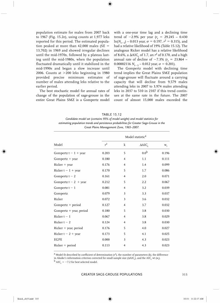
population estimate for males from 2007 back to 1967 (Fig. 15.2e), using counts at 1,977 leks reported for this period. The estimated popula-tion peaked at more than 42,000 males (SE � 13,702) in 1969 and showed irregular declines until the mid-1970s, followed by a plateau last-ing until the mid-1980s, when the population fluctuated dramatically until it stabilized in the mid-1990s and began a slow increase until 2006. Counts at �200 leks beginning in 1980 provided precise minimum estimates of number of males attending leks relative to the earlier period. The best stochastic model for annual rates of change of the population of sage-grouse in the entire Great Plains SMZ is a Gompertz model
with a one-year time lag and a declining time trend of �2.9% per year (rt � 29.245 – 0.430 ln(Nt�1) – 0.013 year, � � 0.197, r2 � 0.315), and had a relative likelihood of 19% (Table 15.12). The analogous Ricker model has a relative likelihood of 8.6%, a �AICc of 1.7, an r2 of 0.170, and a high annual rate of decline of �7.3% (rt � 23.864 – 0.00002116 Nt�1 – 0.012 year, � � 0.201). The Gompertz model with declining time trend implies the Great Plains SMZ population of sage-grouse will fluctuate around a carrying capacity that will decline from 9,579 males attending leks in 2007 to 3,974 males attending leks in 2037 to 510 in 2107 if this trend contin-ues at the same rate in the future. The 2007 count of almost 15,000 males exceeded the
TABLE 15.12Candidate model set (contains 95% of model weight) and model statistics for
estimating population trends and persistence probabilities for Greater Sage-Grouse in theGreat Plains Management Zone, 1965–2007.
Model statistica
Model r2 k ΔAICc wi
Gompertz t � 1 � year 0.203 5 0.0b 0.196
Gompertz � year 0.180 4 1.1 0.111
Ricker � year 0.176 4 1.4 0.099
Ricker t � 1 � year 0.170 5 1.7 0.086
Gompertz t � 2 0.161 4 2.0 0.071
Gompertz t � 2 � year 0.212 5 2.2 0.067
Gompertz t � 1 0.081 4 3.2 0.039
Gompertz 0.079 3 3.3 0.037
Ricker 0.072 3 3.6 0.032
Gompertz � period 0.127 4 3.7 0.032
Gompertz � year, period 0.180 5 3.8 0.030
Ricker t � 1 0.067 4 3.8 0.029
Ricker t � 2 0.124 4 3.8 0.030
Ricker � year, period 0.176 5 4.0 0.027
Ricker t � 2 � year 0.173 5 4.1 0.025
EGPE 0.000 3 4.3 0.023
Ricker � period 0.113 4 4.3 0.023
a Model fi t described by coeffi cient of determination (r2), the number of parameters (k), the difference in Akaike’s information criterion corrected for small sample size (ΔAICc), and the AICc wt (wi).b AICc � �7.2 for best selected model.
Knick_ch15.indd 315Knick_ch15.indd 315 3/1/11 11:22:17 AM3/1/11 11:22:17 AM
STUDIES IN AVIAN BIOLOGY NO. 38 Knick and Connelly316
estimated carrying capacity by 50%. Parametric bootstraps under this model also imply virtually no probability of the population declining below Ne � 50 or Ne � 500 if these rates are main-tained indefinitely. The Ricker model analogous to the best Gompertz model predicts a carrying capacity of 7,647 males in 2007 that rapidly declines to extinction by 2037, with parametric bootstraps predicting 20% likelihood of the pop-ulation declining below Ne � 500 in 30 years and 100% likelihood of numbers below Ne � 50 in 100 years. Multimodel forecasts across all 26 models predict 10% and 11% probabilities of declining below Ne � 50 and Ne � 500 in 30 years (Table 15.6), with standard errors of 5.9% and 5.8%, respectively, and higher (23% and 24%, respectively) probabilities in 100 years (SE � 8.4% and 8.3%, respectively).
Wyoming Basin Management Zone
This SMZ represents sage-grouse populations in parts of Montana, Colorado, Utah, and Wyoming (Fig. 15.1). Most of the sage-grouse in Wyoming and Colorado occur in this SMZ. Four of the five populations delineated within this management zone had data sufficient for analysis.
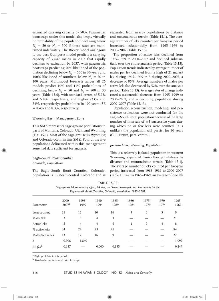
Eagle–South Routt Counties, Colorado, Population
The Eagle–South Routt Counties, Colorado, population is in north-central Colorado and is
separated from nearby populations by distance and mountainous terrain (Table 15.1). The aver-age number of leks counted per five-year period increased substantially from 1965–1969 to 2000–2007 (Table 15.13). The proportion of active leks declined from 1985–1989 to 2000–2007 and declined substan-tially over the entire analysis period (Table 15.13). Population trends indicated by average number of males per lek declined from a high of 21 males/lek during 1965–1969 to 3 during 2000–2007, a decrease of 86%. Average numbers of males per active lek also decreased by 52% over the analysis period (Table 15.13). Average rates of change indi-cated a substantial decrease from 1995–1999 to 2000–2007, and a declining population during 2000–2007 (Table 15.13). Population reconstruction, modeling, and per-sistence estimation were not conducted for the Eagle–South Routt population because of the large number of intervals of �3 successive years dur-ing which no or few leks were counted. It is unlikely the population will persist for 20 years (C. E. Braun, pers. comm.).
Jackson Hole, Wyoming, Population
This is a relatively isolated population in western Wyoming, separated from other populations by distance and mountainous terrain (Table 15.1). The average number of leks counted per five-year period increased from 1965–1969 to 2000–2007 (Table 15.14). In 1965–1969, an average of one lek
TABLE 15.13Sage-grouse lek monitoring effort, lek size, and trends averaged over 5-yr periods for the
Eagle–south Routt Counties, Colorado, population, 1965–2007.
Parameter2000–2007
a1995–1999
1990–1994
1985–1989
1980–1984
1975–1979
1970–1974
1965–1969
Leks counted 21 15 20 16 3 0 5 9
Males/lek 3 3 4 3 — — — 21
Active leks 5 4 4 6 1 0 4 8
% active leks 34 24 23 41 — — — 84
Males/active lek 13 12 16 9 — — — 27
λ 0.906 1.840 — — — — — 1.092
SE (λ)b 0.137 — 0.000 0.155 — — — 0.247
a Eight yr of data in this period.b Standard error for annual rate of change.
Knick_ch15.indd 316Knick_ch15.indd 316 3/1/11 11:22:17 AM3/1/11 11:22:17 AM

GREATER SAGE-GROUSE POPULATIONS 317
TABLE 15.14Sage-grouse lek monitoring effort, lek size, and trends averaged over 5-yr periods
for the Jackson Hole, Wyoming, population, 1965–2007.
Parameter2000–2007
a1995–1999
1990–1994
1985–1989
1980–1984
1975–1979
1970–1974
1965–1969
Leks counted 6 8 7 5 1 — — 1
Males/lek 16 10 28 19 — — — —
Active leks 6 6 7 4 0 — — 0
% active leks 92 73 100 77 — — — —
Males/active lek 18 14 28 25 — — — —
λ 1.075 0.851 1.029 1.217 — — — —
SE (λ)b 0.158 0.346 0.223 0.371 — — — —
a Eight yr of data in this period.b Standard error for annual rate of change.
per five-year period was censused, but by 2005–2007, an average of six leks were counted. The proportion of active leks fluctuated over the assessment period (Table 15.14). Population trends, as indicated by average number of males per lek, declined from 28 in 1990–1994 to 16 in 2000–2007. Average number of males per active lek also declined over the assessment period (Table 15.14). Average rates of change were 1.0 for one of the four periods for which data could be analyzed. However, the rate of change was 1.0 in the 1995–1999 analysis period and �1.0 in the 2000–2007 period, sug-gesting an increasing population over this period (Table 15.14). Population reconstruction was only feasible for 1986–2007 for this population, but the estimated annual rates of change implied that the 2007 count of �129 males (SE � 44) attending nine leks was typical of counts during this time, with the maximum count of 200 occurring around 1990. Standard errors prior to 1998 were quite large (Fig. 15.3a), but the population had a pattern of declining counts with a count of 200 breeding males from 1988–1995 followed by a substantial decline to half that number in the late 1990s and early 2000s. None of the 26 models garnered �10% relative likelihood, with the simplest models (exponential growth with process error, Gompertz, and Ricker) all showing similar relative likelihoods of 6–8% (Table 15.15).
The simple exponential growth with process error model estimated the annual rate of change for this population averaged �2.2%, which leads to relatively high likelihoods of popula-tions declining below Ne � 50. Estimated male counts were already below 200, and probability of long-term persistence for Ne � 500 was 0%. Multimodel forecasts across all 26 models esti-mated 11% and 27% probabilities of declining below Ne � 50 in 30 and 100 years, respectively (Table 15.6).
Middle Park, Colorado, Population
This population occurs in north-central Colorado and is separated from adjacent populations by distance and mountainous terrain (Table 15.1). The average number of leks counted per five-year period increased from 7 to 35 from 1965–1969 to 1990–1994, and then decreased to 17 by 2000–2007 (Table 15.16). The proportion of active leks declined from 1965–1969 to 1995–1999, and then increased in 2000–2007 (Table 15.16). Population trends indicated by average number of males per lek declined by 40% from 1965–1969 to 1995–1999, and then increased by 78% from 1995–1999 to 2000–2007. Average number of males per active lek remained relatively constant over the assess-ment period (Table 15.16). In contrast to males/lek data, average rates of change were 1.0 for five of the eight analysis periods and
Knick_ch15.indd 317Knick_ch15.indd 317 3/1/11 11:22:17 AM3/1/11 11:22:17 AM

b. Middle Park, Colorado
a. Jackson Hole, Wyoming
c. Wyoming Basin
Figure 15.3. Population reconstructions for Wyoming Basin populations and Wyoming Basin Management Zone: (a) Jackson Hole, Wyoming; (b) Middle Park, Colorado; (c) Wyoming basin; (d) Wyoming Basin Management Zone.
Knick_ch15.indd 318Knick_ch15.indd 318 3/1/11 11:22:17 AM3/1/11 11:22:17 AM

GREATER SAGE-GROUSE POPULATIONS 319
indicated a generally decreasing population in 2000–2007 (Table 15.16). Moreover, rate of change declined by 21% between the 1995–1999 and 2000–2007 analysis periods and was 1.0 for 2000–2007. Population reconstruction was only feasible for 1987–2007 for this population, but esti-mated annual rates of change implied the 2007
count of a minimum of 190 males (SE � 52) attending nine leks was typical of counts dur-ing this time, with maximum counts of 300 occurring around 1990 and 2001 separated by a decline to 100 in mid-1990s. Standard errors grew from 27% of the estimate in 2007 to approximately equal to it in 1987 (Fig. 15.3b), but the population showed only a simple pattern
d. Wyoming Basin Management Zone
Figure 15.3. (Continued)
TABLE 15.15Candidate model set (contains 95% of model weight) and model statistics for
estimating population trends and persistence probabilities for Greater Sage-Grouse in the Jackson Hole, Wyoming, population, 1965–2007.
Model statistica
Model r2 k ΔAIC wi
EGPE 0.000 3 0.0b 0.170
Gompertz t � 2 0.126 4 0.3 0.148
Ricker 0.125 4 0.3 0.145
Ricker t � 2 0.112 4 0.6 0.126
Gompertz 0.111 4 0.6 0.125
Gompertz t � 1 0.049 4 1.9 0.066
Ricker t � 1 0.034 4 2.2 0.057
Ricker � year 0.162 5 2.7 0.043
Gompertz t � 2 � year 0.148 5 3.1 0.037
Gompertz � year 0.136 5 3.3 0.032
Ricker t � 2 � year 0.123 5 3.6 0.028
a Model fi t described by coeffi cient of determination (r2), the number of parameters (k), the difference in Akaike’s information criterion corrected for small sample size (�AICc), and the AICc wt (wi).b AICc � 5.4 for best selected model.
Knick_ch15.indd 319Knick_ch15.indd 319 3/1/11 11:22:18 AM3/1/11 11:22:18 AM

STUDIES IN AVIAN BIOLOGY NO. 38 Knick and Connelly320
of increasing counts from around 200 breeding males to 300, followed by a substantial decline to half that number in the mid-1990s and a gen-eral increase through the 2000s. The Middle Park sage-grouse population was one of three in which six models had about 10% relative likelihoods (exponential growth with process error, Gompertz, and Ricker;
Table 15.17). The simple exponential growth with process error model estimated the annual rate of change for this population is close to 0, which leads to moderate likelihoods (9–30%) of declining below Ne � 50 in 30 or 100 years. Estimated male counts were already below 200, and probability of long-term persistence unlikely given the best fit model. Multimodel
TABLE 15.16Sage-grouse lek monitoring effort, lek size, and trends averaged over 5-yr periods
for the Middle Park, Colorado, population, 1965–2007.
Parameter2000–2007
a1995–1999
1990–1994
1985–1989
1980–1984
1975–1979
1970–1974
1965–1969
Leks counted 17 21 35 26 9 8 5 7
Males/lek 16 9 5 7 14 23 18 15
Active leks 15 13 17 15 6 8 4 6
% active leks 90 66 49 58 71 96 96 84
Males/active lek 17 14 11 12 20 24 19 17
λ 0.978 1.241 0.916 0.729 1.412 0.834 0.714 1.095
SE (λ)b 0.080 0.197 0.149 0.122 1.217 0.271 0.182 0.259
a Eight yr of data in this period.b Standard error for annual rate of change.
TABLE 15.17Candidate model set (contains 95% of model weight) and model statistics for
estimating population trends and persistence probabilities for Greater Sage-Grouse in the Middle Park, Colorado, population, 1986–2007.
Model statistica
Model r2 k ΔAIC wi
Gompertz 0.156 4 0.0b 0.228
EGPE 0.000 3 0.4 0.190
Ricker 0.134 4 0.5 0.179
Gompertz � year 0.195 5 2.3 0.070
Gompertz t � 2 0.041 4 2.4 0.068
Ricker � year 0.183 5 2.6 0.061
Ricker t � 1 0.018 4 2.9 0.054
Gompertz t � 1 0.017 4 2.9 0.054
Ricker t � 2 0.009 4 3.0 0.050
a Model fi t described by coeffi cient of determination (r2), the number of parameters (k), the difference in Akaike’s information criterion corrected for small sample size (�AICc), and the AICc wt (wi).b AICc � 9.1 for best selected model.
Knick_ch15.indd 320Knick_ch15.indd 320 3/1/11 11:22:18 AM3/1/11 11:22:18 AM

GREATER SAGE-GROUSE POPULATIONS 321
forecast across all 26 models projected 3% and 7% probabilities, respectively, of the population declining below Ne � 50 in 30 and 100 years (Table 15.6).
Wyoming Basin Population
This population occupies much of Wyoming as well as part of southern Montana, northeastern Utah, and northern Colorado. It is separated from other populations by distance and topo-graphic features (Table 15.1). The average number of leks counted per five-year period increased substantially from 1965–1969 to 2000–2007 (Table 15.18). The proportion of active leks fluctuated slightly, but remained stable over the assessment period (Table 15.18). Population trends, as indicated by average number of males per lek, declined by 17% from 1965–1969 to 2000–2007. However, lek size decreased by 48% from 1965–1969 to 1995–1999 and then increased by 60% from 1995–1999 to 2000–2007. Average number of males per active lek also had the same pattern and an overall decline of 21% over the assessment period (Table 15.18). Average rates of change were 1.0 for four of the eight analysis periods. Average rates of change were 1.0 during the 1980s and early 1990s, and then increased substantially during 1995–1999. However,
average rates of change declined by 6% between the last two analysis periods, although both values remained at or above 1.0 for these periods (Table 15.18). From a minimum population estimate of 40,166 males (SE � 1,401) in 2007 based on counts at 1,298 leks, we reconstructed a minimum popula-tion estimate for males from 2007 back to 1965 (Fig. 15.3c), using counts at 1,670 leks reported for this 43-year period. The estimated minimum population grew from 1965 to peak at more than 130,000 males in 1969, and showed regular declines and peaks at 9- to 10-year intervals until the present, with an overall declining trend and the relative magnitude of the difference between peaks and troughs decreasing. Counts at more than 300 leks beginning in 1980 provided more precise minimum estimates of number of males attending leks than the earlier periods. The best stochastic model for the annual rates of change of the Wyoming Basin population is a Gompertz model with a one-year time lag and a declining time trend of �3.4% per year (rt � 23.017 – 0.294 ln(Nt�1) – 0.010 year, � � 0.152, r2 � 0.188); this model has a relative likelihood of 16% (Table 15.19). The analogous Ricker model has a relative likelihood of 6.4%, a �AICc of 1.8, an r2 of 0.150, and a high annual rate of declineof �10.5% (rt � 14.255 – 0.0000445 Nt�1 – 0.00707 year, � � 0.1554).
TABLE 15.18Sage-grouse lek monitoring effort, lek size, and trends averaged over 5-yr periods for the
Wyoming basin population, 1965–2007.
Parameter2000–2007
a1995–1999
1990–1994
1985–1989
1980–1984
1975–1979
1970–1974
1965–1969
Leks counted 1149 752 610 515 330 184 137 130
Males/lek 24 15 16 19 23 25 24 29
Active leks 807 501 431 377 248 137 97 91
% active leks 70 67 71 74 75 74 72 69
Males/active lek 33 22 23 25 30 33 34 42
λ 1.061 1.118 0.856 0.986 0.915 1.046 0.928 1.039
SE (λ)b 0.025 0.082 0.038 0.049 0.055 0.072 0.076 0.098
a Eight yr of data in this period.b Standard error for annual rate of change.
Knick_ch15.indd 321Knick_ch15.indd 321 3/1/11 11:22:18 AM3/1/11 11:22:18 AM

STUDIES IN AVIAN BIOLOGY NO. 38 Knick and Connelly322
The Gompertz model with declining time trend implies the Wyoming Basin population of sage-grouse will fluctuate around an estimated carrying capacity that will decline from 20,980 males attending leks in 2007 to 7,545 males attending leks in 2037 to 2 in 2107 if this trend continues at the same rate in the future. The Ricker model analogous to the best Gompertz model predicts a carrying capacity of 15,079 males in 2007 that declines to extinction by 2037. Multimodel forecasts across all 26 models predict 10% and 11% probabilities of the Wyoming Basin minimum population index declining below Ne � 50 and Ne � 500, respectively, in 100 years (Table 15.6).
Comprehensive Analysis of All Leks in the Management Zone
The average number of leks counted per five-year period increased substantially over the assess-ment period (Table 15.20). In 1965–1969, an aver-age of 138 leks per year was censused, but by 2005–2007, an average of 1,321 leks per year was counted, an increase of 857%. The proportion of active leks decreased slightly over the assessment period, averaging between 70% and 72% from 1965–1989 but declining to 65% by 2005–2007 (Table 15.20). Population trends, as indicated by average number of males per lek, decreased over the assessment period by
TABLE 15.19Candidate model set (contains 95% of model weight) and model statistics for
estimating population trends and persistence probabilities for Greater Sage-Grouse in the Wyoming basin population, 1965–2007.
Model statistica
Model r2 k ΔAICc wi
Gompertz t � 1 � year 0.188 5 0.0b 0.162
Gompertz t � 1 � period 0.171 4 0.8 0.108
Gompertz t � 1 0.102 4 1.5 0.075
Gompertz t � 1 � year, period 0.211 5 1.5 0.078
Gompertz t � 2 � year 0.153 6 1.7 0.070
Ricker t � 1 0.097 4 1.8 0.066
Ricker t � 1 � year 0.150 5 1.8 0.064
Gompertz t � 2 0.083 5 2.4 0.049
Gompertz t � 2 � period 0.135 5 2.5 0.046
Ricker t � 1 � period 0.134 5 2.6 0.045
Gompertz t � 2 � year, period 0.174 6 3.3 0.031
EGPE 0.000 3 3.5 0.028
Gompertz 0.055 3 3.6 0.027
Ricker 0.054 3 3.6 0.027
Ricker t � 2 0.055 4 3.6 0.027
Ricker t � 1 � year, period 0.156 6 4.2 0.020
Period 0.018 3 5.1 0.013
Gompertz � period 0.065 4 5.6 0.010
a Model fi t described by coeffi cient of determination (r2), the number of parameters (k), the difference in Akaike’s information criterion corrected for small sample size (ΔAICc), and the AICc wt (wi).b AICc � �28.1 for best selected model.
Knick_ch15.indd 322Knick_ch15.indd 322 3/1/11 11:22:18 AM3/1/11 11:22:18 AM
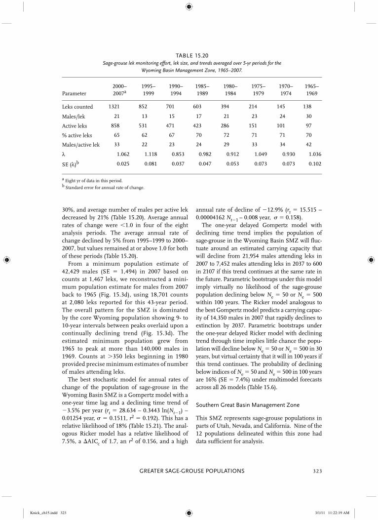
GREATER SAGE-GROUSE POPULATIONS 323
30%, and average number of males per active lek decreased by 21% (Table 15.20). Average annual rates of change were 1.0 in four of the eight analysis periods. The average annual rate of change declined by 5% from 1995–1999 to 2000–2007, but values remained at or above 1.0 for both of these periods (Table 15.20). From a minimum population estimate of 42,429 males (SE � 1,494) in 2007 based on counts at 1,467 leks, we reconstructed a mini-mum population estimate for males from 2007 back to 1965 (Fig. 15.3d), using 18,701 counts at 2,080 leks reported for this 43-year period. The overall pattern for the SMZ is dominated by the core Wyoming population showing 9- to 10-year intervals between peaks overlaid upon a continually declining trend (Fig. 15.3d). The estimated minimum population grew from 1965 to peak at more than 140,000 males in 1969. Counts at �350 leks beginning in 1980 provided precise minimum estimates of number of males attending leks. The best stochastic model for annual rates of change of the population of sage-grouse in the Wyoming Basin SMZ is a Gompertz model with a one-year time lag and a declining time trend of �3.5% per year (rt � 28.634 – 0.3443 ln(Nt�1) – 0.01254 year, � � 0.1511, r2 � 0.192). This has a relative likelihood of 18% (Table 15.21). The anal-ogous Ricker model has a relative likelihood of 7.5%, a �AICc of 1.7, an r2 of 0.156, and a high
annual rate of decline of �12.9% (rt � 15.515 – 0.00004162 Nt�1 – 0.008 year, � � 0.158). The one-year delayed Gompertz model with declining time trend implies the population of sage-grouse in the Wyoming Basin SMZ will fluc-tuate around an estimated carrying capacity that will decline from 21,954 males attending leks in 2007 to 7,452 males attending leks in 2037 to 600 in 2107 if this trend continues at the same rate in the future. Parametric bootstraps under this model imply virtually no likelihood of the sage-grouse population declining below Ne � 50 or Ne � 500 within 100 years. The Ricker model analogous to the best Gompertz model predicts a carrying capac-ity of 14,350 males in 2007 that rapidly declines to extinction by 2037. Parametric bootstraps under the one-year delayed Ricker model with declining trend through time implies little chance the popu-lation will decline below Ne � 50 or Ne � 500 in 30 years, but virtual certainty that it will in 100 years if this trend continues. The probability of declining below indices of Ne � 50 and Ne � 500 in 100 years are 16% (SE � 7.4%) under multimodel forecasts across all 26 models (Table 15.6).
Southern Great Basin Management Zone
This SMZ represents sage-grouse populations in parts of Utah, Nevada, and California. Nine of the 12 populations delineated within this zone had data sufficient for analysis.
TABLE 15.20Sage-grouse lek monitoring effort, lek size, and trends averaged over 5-yr periods for the
Wyoming Basin Management Zone, 1965–2007.
Parameter2000–2007
a1995–1999
1990–1994
1985–1989
1980–1984
1975–1979
1970–1974
1965–1969
Leks counted 1321 852 701 603 394 214 145 138
Males/lek 21 13 15 17 21 23 24 30
Active leks 858 531 471 423 286 151 101 97
% active leks 65 62 67 70 72 71 71 70
Males/active lek 33 22 23 24 29 33 34 42
λ 1.062 1.118 0.853 0.982 0.912 1.049 0.930 1.036
SE (λ)b 0.025 0.081 0.037 0.047 0.053 0.073 0.073 0.102
a Eight yr of data in this period.b Standard error for annual rate of change.
Knick_ch15.indd 323Knick_ch15.indd 323 3/1/11 11:22:19 AM3/1/11 11:22:19 AM

STUDIES IN AVIAN BIOLOGY NO. 38 Knick and Connelly324
Mono Lake, California–Nevada, Population
This population straddles the California and Nevada border and is separated from other popu-lations by distance and topography (Table 15.1). The average number of leks counted per five-year period increased substantially from 1965–1969 to 2000–2007 (Table 15.22). The proportion of active leks fluctuated but remained relatively stable over the assessment period (Table 15.22). Population trends, as indicated by average number of males per lek, declined 35% from 1965–1969 to 2000–2007. The average number of males per active lek also declined by 41% over the assessment period (Table 15.22). Average rates of change were 1.0 for three of the eight analysis periods (Table 15.22).
Average rate of change declined by 45% between the last two analysis periods, but values re mained at or above 1.0 for both of these periods(Table 15.22). From a minimum population estimate of 274 males (SE � 101) in 2007 based on counts at 11 of 19 leks, we reconstructed a minimum pop-ulation estimate for males from 2007 back to 1965 (Fig. 15.4a), using 361 counts at leks reported for this 43-year period. The overall pat-tern for the population shows irregular fluctua-tions between peaks in 1970 and 1987 of 520–670 males with lows above 100 (Fig. 15.4a) and no consistent long-term trend over the 40-year period. Since 1991, minimum counts have been trending upward. Counts at almost all the leks in
TABLE 15.21Candidate model set (contains 95% of model weight) and model statistics for
estimating population trends and persistence probabilities for Greater Sage-Grouse in theWyoming Basin Management Zone, 1965–2007.
Model statistica
Model r2 k ΔAICc wi
Gompertz t � 1 � year 0.192 5 0.0b 0.177
Gompertz t � 2 0.168 4 1.2 0.099
Gompertz t � 2 � year 0.215 5 1.5 0.085
Gompertz t � 1 � year, period 0.156 6 1.7 0.075
Ricker t � 1 � year 0.156 5 1.7 0.075
Gompertz t � 1 0.097 4 1.9 0.068
Ricker t � 1 0.095 4 2.1 0.063
Ricker t � 2 0.134 4 2.7 0.045
Gompertz t � 1 � period 0.078 5 2.8 0.044
Gompertz t � 2 � period 0.129 5 3.0 0.040
Gompertz t � 2 � year, period 0.175 6 3.4 0.032
EGPE 0.000 3 3.7 0.028
Ricker t � 1 � period 0.052 5 3.9 0.025
Gompertz 0.050 3 4.0 0.024
Ricker 0.050 3 4.0 0.024
Ricker t � 2 � year 0.161 5 4.1 0.023
Period 0.017 3 5.3 0.012
Ricker t � 1 � year, period 0.065 6 5.8 0.010
a Model fi t described by coeffi cient of determination (r2), the number of parameters (k), the difference in Akaike’s information criterion corrected for small sample size (�AICc), and the AICc wt (wi).b AICc � �26.5 for best selected model.
Knick_ch15.indd 324Knick_ch15.indd 324 3/1/11 11:22:19 AM3/1/11 11:22:19 AM

GREATER SAGE-GROUSE POPULATIONS 325
recent years have provided more precise mini-mum estimates of number of males attending leks than earlier counts. The best population growth models for the Mono Lake population were a simple Gompertz (rt � 3.545 – 0.677 ln(Nt), � � 0.447, r2 � 0.332, 29% relative likelihood) or a simple Ricker (15% relative likelihood) or simple Gompertz with time, period, or time � period (14% to 6% relative like-lihoods, Table 15.23). The Gompertz model explained 33% of the variation in growth rates, as did the Gompertz model with declining time trend (rt � 4.935 – 0.68 ln(Nt�1) – 0.00069 year, � � 0.4646, r2 � 0.332; Table 15.23), and both forecast carrying capacities under 200 males (187 for Gompertz and declining K in 2007, 2037, and 2107 and 183, 178, and 165, respectively, under Gompertz with time trend). Long-term persist-ence above Ne � 500 is clearly unlikely, but short-term probability of declining below Ne � 50 is 15% in 30 years and 38% in 100 years across mul-tiple models (Table 15.6).
South Mono Lake, California, Population
This population occurs in eastern California and is separated from other populations by distance and topography (Table 15.1). The average number of leks counted per five-year period increased some-what from 1965–1969 to 2000–2007 (Table 15.24). The proportion of active leks increased from 1965–1969 to 1985–1989 and declined slightly
thereafter (Table 15.24). Population trends, as indicated by average number of males per lek, increased by 218% from 1965–1969 to 1985–1989 but declined by 49% from 1985–1989 to 2000–2007. Average number of males per active lek followed the same pattern over the assessment period (Table 15.24). Average rates of change were 1.0 for three of the eight analysis periods and indicated a decreasing population during the mid- to late 1980s and early 1990s (Table 15.24). Average rate of change was relatively stable over the last two analysis periods, and values re -mained at or above 1.0 for both of these periods (Table 15.24). We used 2005 as the base year to reconstruct this population because the most leks (N � 32) were counted in that year of any available (1965–2007). The estimated minimum number of males attending leks in the population was 459 (SE � 61), and the estimated rates of increase were used to reconstruct the population back to 1965 and for-ward to 2007 based on the estimated annual rates of change. Standard errors were large prior to 1985 (Fig. 15.4b), and the population showed no obvious pattern through time except a ten-dency to remain between 200 and 600 males attending leks. South Mono Lake grouse population was modeled best by a Gompertz model with no time lags (50% relative likelihood), with two other related Gompertz models strongly sup-ported by the data (Table 15.25). Male counts at
TABLE 15.22Sage-grouse lek monitoring effort, lek size, and trends averaged over 5-yr periods for the
Mono Lake, California–Nevada, population, 1965–2007.
Parameter2000–2007
a1995–1999
1990–1994
1985–1989
1980–1984
1975–1979
1970–1974
1965–1969
Leks counted 24 13 17 18 14 13 12 5
Males/lek 15 9 17 16 17 20 24 23
Active leks 19 7 12 12 8 10 10 4
% active leks 81 56 70 69 58 75 87 75
Males/active lek 19 17 24 23 29 27 27 32
λ 1.050 1.912 0.923 1.058 0.964 1.134 0.968 1.486
SE (λ)b 0.143 0.677 0.169 0.160 0.256 0.390 0.263 0.838
a Eight yr of data in this period.b Standard error for annual rate of change.
Knick_ch15.indd 325Knick_ch15.indd 325 3/1/11 11:22:19 AM3/1/11 11:22:19 AM

c. Northeast interior Utah
b. South Mono Lake, California
a. Mono Lake, California–Nevada
Figure 15.4. Population reconstructions for Southern Great Basin popu-lations and Southern Great Basin Management Zone: (a) Mono Lake, California-Nevada; (b) south Mono Lake, California; (c) northeast interior Utah; (d) Sanpete–Emery Counties, Utah; (e) south-central Utah; (f) Summit–Morgan Counties, Utah; (g) Toole-Juab Counties, Utah; (h) Southern Great Basin; (i) Southern Great Basin Management Zone.
Knick_ch15.indd 326Knick_ch15.indd 326 3/1/11 11:22:19 AM3/1/11 11:22:19 AM

f. Summit–Morgan Counties, Utah
e. South central Utah
d. Sanpete–Emery Counties Utah
Figure 15.4. (Continued)
Knick_ch15.indd 327Knick_ch15.indd 327 3/1/11 11:22:20 AM3/1/11 11:22:20 AM

i. Southern Great Basin Management Zone
h. Southern Great Basin
g. Tooele–Juab Counties, Utah
Figure 15.4. (Continued)
Knick_ch15.indd 328Knick_ch15.indd 328 3/1/11 11:22:20 AM3/1/11 11:22:20 AM

TABLE 15.23Candidate model set (contains 95% of model weight) and model statistics for
estimating population trends and persistence probabilities for Greater Sage-Grouse in the Mono Lake, California–Nevada, population, 1965–2007.
Model statistica
Model r2 k ΔAICc wi
Gompertz 0.332 3 0.0b 0.292
Ricker 0.229 3 1.3 0.153
Gompertz � year 0.332 4 1.4 0.143
Gompertz � period 0.342 4 2.3 0.092
Gompertz � year, period 0.364 5 3.1 0.062
Ricker � year 0.229 4 3.2 0.058
Ricker � period 0.233 4 3.8 0.044
Ricker � year, period 0.254 5 4.3 0.035
Gompertz t � 1 0.069 4 5.7 0.017
Ricker t � 1 0.062 4 6.0 0.015
Gompertz t � 2 0.059 4 6.1 0.014
EGPE 0.000 3 6.2 0.013
Ricker t � 2 0.057 4 6.2 0.013
a Model fi t described by coeffi cient of determination (r2), the number of parameters (k), the difference in Akaike’s information criterion corrected for small sample size (ΔAICc), and the AICc wt (wi).b AICc � 38.0 for best selected model.
TABLE 15.24Sage-grouse lek monitoring effort, lek size, and trends averaged over 5-yr periods for the
South Mono Lake, California, population, 1965–2007.
Parameter2000–2007
a1995–1999
1990–1994
1985–1989
1980–1984
1975–1979
1970–1974
1965–1969
Leks counted 10 11 11 10 9 9 8 6
Males/lek 18 19 19 35 14 12 16 11
Active leks 8 9 10 9 6 7 6 4
% active leks 83 83 84 90 74 78 72 74
Males/active lek 22 22 22 39 19 16 21 16
λ 1.080 1.063 0.971 0.995 1.267 1.048 0.846 1.683
SE (λ)b 0.191 0.170 0.219 0.097 0.367 0.321 0.155 0.831
a Eight yr of data in this period.b Standard error for annual rate of change.
Knick_ch15.indd 329Knick_ch15.indd 329 3/1/11 11:22:21 AM3/1/11 11:22:21 AM

STUDIES IN AVIAN BIOLOGY NO. 38 Knick and Connelly330
south Mono Lake have already been below 200, and probability of long-term persistence is low, but the multimodel inference for short-term (Ne � 50) persistence is more likely (i.e., 1% probability of declining below Ne � 50; Table 15.6).
Northeast Interior Utah Population
This population is in northeast Utah and is sepa-rated from adjacent populations by distance and topography (Table 15.1). The average number of leks counted per five-year period increased substantially
from 1965–1969 to 2000–2007 (Table 15.26). The proportion of active leks declined by 21% over the assessment period (Table 15.26). Population trends, as indicated by average number of males per lek, declined by 47% from 1970–1974 to 2000–2007. The average number of males per active lek also declined by 26% over the same period (Table 15.26). Average rates of change were 1.0 for three of eight analysis periods and indicated a decreasing population during the mid- to late 1980s and early 1990s (Table 15.26). Average rate of change increased during the 1990s but declined 8% between the last two analysis
TABLE 15.25Candidate model set (contains 95% of model weight) and model statistics for
estimating population trends and persistence probabilities for Greater Sage-Grouse in the South Mono Lake, California, population, 1965–2007.
Model statistica
Model r2 k ΔAICc wi
Gompertz 0.331 3 0.0b 0.499
Gompertz � period 0.342 4 1.8 0.198
Gompertz � year 0.332 4 2.5 0.146
Gompertz � year, period 0.364 5 3.1 0.106
a Model fi t described by coeffi cient of determination (r2), the number of parameters (k), the difference in Akaike’s information criterion corrected for small sample size (ΔAICc), and the AICc wt (wi).b AICc � 55.7 for best selected model.
TABLE 15.26Sage-grouse lek monitoring effort, lek size, and trends averaged over 5-yr periods for the
northeast interior Utah population, 1965–2007.
Parameter2000–2007
a1995–1999
1990–1994
1985–1989
1980–1984
1975–1979
1970–1974
1965–1969
Leks counted 25 16 18 14 15 20 13 2
Males/lek 10 8 9 15 11 22 19 —
Active leks 15 9 13 11 10 19 9 1
% active leks 60 65 75 79 62 93 76 —
Males/active lek 17 12 13 19 18 23 23 —
λ 1.116 1.211 0.885 0.892 1.120 0.924 1.144 —
SE (λ)b 0.195 0.213 0.190 0.170 0.320 0.169 0.240 —
a Eight yr of data in this period.b Standard error for annual rate of change.
Knick_ch15.indd 330Knick_ch15.indd 330 3/1/11 11:22:21 AM3/1/11 11:22:21 AM
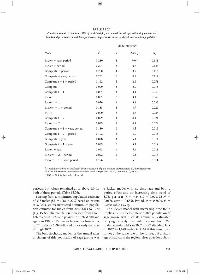
GREATER SAGE-GROUSE POPULATIONS 331
periods, but values remained at or above 1.0 for both of these periods (Table 15.26). Starting from a minimum population estimate of 338 males (SE � 108) in 2007 based on counts at 32 leks, we reconstructed a minimum popula-tion estimate for males from 2007 back to 1970 (Fig. 15.4c). The population increased from about 476 males in 1970 and peaked in 1976 at 600 and again in 1986 at 750 males before reaching a low of 77 males in 1994 followed by a steady increase through 2007. The best stochastic model for the annual rates of change of this population of sage-grouse was
a Ricker model with no time lags and both a period effect and an increasing time trend of 3.7% per year (rt � �34.817 � 0.001322 Nt � 0.0176 year � 0.6558 Period, � � 0.2809, r2 � 0.280; Table 15.27). The Ricker model with increasing time trend implies the northeast interior Utah population of sage-grouse will fluctuate around an estimated carrying capacity that will increase from 358 males attending leks in 2007 to 757 attending leks in 2037 to 1,688 males in 2107 if this trend con-tinues at the same rate in the future, but a short-age of habitat in the region raises questions about
TABLE 15.27Candidate model set (contains 95% of model weight) and model statistics for estimating population
trends and persistence probabilities for Greater Sage-Grouse in the northeast interior Utah population.
Model statistica
Model r2 k ΔAICc wi
Ricker � year, period 0.280 5 0.0b 0.185
Ricker � period 0.204 4 0.8 0.126
Gompertz � period 0.200 4 0.9 0.116
Gompertz � year, period 0.261 5 0.9 0.117
Gompertz t � 1 � period 0.162 5 2.6 0.051
Gompertz 0.090 3 2.9 0.043
Gompertz t � 1 0.085 4 3.1 0.040
Ricker 0.085 3 3.1 0.040
Ricker t � 1 0.076 4 3.4 0.033
Ricker t � 1 � period 0.135 5 3.7 0.029
EGPE 0.000 3 3.8 0.028
Gompertz t � 2 0.059 4 4.1 0.024
Ricker t � 2 0.059 4 4.1 0.024
Gompertz t � 1 � year, period 0.180 6 4.5 0.019
Gompertz t � 2 � period 0.102 5 5.0 0.015
Gompertz � year 0.098 4 5.1 0.014
Gompertz t � 1 � year 0.099 5 5.1 0.014
Ricker � year 0.093 4 5.4 0.013
Ricker t � 2 � period 0.092 5 5.4 0.013
Ricker t � 1 � year, period 0.156 6 5.6 0.011
a Model fi t described by coeffi cient of determination (r2), the number of parameters (k), the difference in Akaike’s information criterion corrected for small sample size (ΔAICc), and the AICc wt (wi).b AICc � 22.5 for best selected model.
Knick_ch15.indd 331Knick_ch15.indd 331 3/1/11 11:22:21 AM3/1/11 11:22:21 AM

STUDIES IN AVIAN BIOLOGY NO. 38 Knick and Connelly332
the potential for this forecast to be realized. A parametric bootstrap based on the Ricker model with increasing time trend, which has a 19% rela-tive likelihood, infers that there is virtually no chance of the population declining below Ne � 50 but declining below Ne � 500 is possible within 100 years (37% relative probability). Multimodel forecasts across all 26 models predict low proba-bilities of declining below population indices of Ne � 50 in 30 and 100 years (1% and 9%, respec-tively; Table 15.6) but higher probabilities of declining below Ne � 500 (52% and 79% in 30 and 100 years, respectively; Table 15.6).
Sanpete–Emery Counties, Utah, Population
This is an isolated population in central Utah and is separated from other populations by distance and topography (Table 15.1). The average number of leks counted per five-year period was relatively stable from 1965–1969 to 2000–2007 (Table 15.28). In 1965–1969 an average of one lek per five-year period was censused, and by 2000–2007 an aver-age of three leks were counted. The average number of active leks counted per five-year period was also relatively stable. The proportion of active leks declined over the assessment period but total leks counted was quite low (Table 15.28). Population trends, as indicated by average number of males per lek, declined by 30% from 1985–1989 to 2000–2007. Average number of males per active lek
fluctuated considerably over the assessment period (Table 15.28). Average rates of change were �1.0 for all four analysis periods and gen-erally suggested a stable to increasing popula-tion (Table 15.28). The average rate of change increased by 33% between the last two analysis periods. A simple Gompertz model without time lags and a Gompertz with period effect were the most descriptive models for this population (Table 15.29, Fig. 15.4d). These two models together represented half of the likelihood based on model weights, but comparable Ricker models were second most likely. Multimodel forecasts predict high probabil-ities of this population declining below Ne � 50 in 30 and 100 years (78% and 99%, respectively; Table 15.6).
South Central Utah Population
This is an isolated population in south central Utah and is separated from other populations by distance and mountainous terrain (Table 15.1). The average number of leks counted per five-year period increased from 1965–1969 to 2000–2007 (Table 15.30). The proportion of active leks remained relatively stable over the assessment period (Table 15.30). Population trends, as indicated by average number of males per lek, fluctuated but remained relatively stable from 1965–1969 to 2000–2007. Average number of males per active lek followed the same
TABLE 15.28Sage-grouse lek monitoring effort, lek size, and trends averaged over 5-yr periods for the
Sanpete–Emery Counties, Utah, population, 1965–2007.
Parameter2000–2007
a1995–1999
1990–1994
1985–1989
1980–1984
1975–1979
1970–1974
1965–1969
Leks counted 3 3 3 2 0 1 3 1
Males/lek 7 5 5 10 — — — —
Active leks 2 1 3 2 — — — —
% active leks 60 33 85 100 — — — —
Males/active lek 11 16 6 10 — — — —
λ 1.430 1.072 1.732 1.089 — — — —
SE (λ)b 0.609 0.000 1.438 0.580 — — — —
a Eight yr of data in this period.b Standard error for annual rate of change.
Knick_ch15.indd 332Knick_ch15.indd 332 3/1/11 11:22:22 AM3/1/11 11:22:22 AM

GREATER SAGE-GROUSE POPULATIONS 333
pattern over the assessment period (Table 15.30). Average rates of change were 1.0 for three of the eight analysis periods but generally suggested a stable to increasing population (Table 15.30). Aver-age rate of change declined 9% between the last two analysis periods, but values remained at or above 1.0 for both of these periods (Table 15.30). We reconstructed a minimum population esti-mate for males from a minimum 2007 population estimate of 1,219 males (SE � 220) based on counts at 42 leks to 1967 (Fig. 15.4e), using 57 lek
counts reported for this period. Counts were high-est in 1969 and 1970 at just over 2,000 males, but the population has generally fluctuated around 1,000 over the period from 1971 to 2007. The best stochastic model for the annual rates of change of the south central Utah population of sage-grouse was a Gompertz model with no time lags, period effects, or time trend (rt � 2.4099 – 0.3542ln(Nt), � � 0.2776, r2 � 0.209; Table 15.31). Based on this model, the estimated carrying capacity for this population was 901 males.
TABLE 15.29Candidate model set (contains 95% of model weight) and model statistics for
estimating population trends and persistence probabilities for Greater Sage-Grouse in the Sanpete–Emery Counties, Utah, population, 1965–2007.
Model statistica
Model r2 k ΔAICc wi
Gompertz 0.311 4 0.0 0.499
Ricker 0.247 4 1.8 0.204
Gompertz � year 0.329 5 2.6 0.133
Ricker � year 0.258 5 4.6 0.049
EGPE 0.000 3 4.7 0.049
Gompertz t � 1 0.022 4 7.0 0.015
a Model fi t described by coeffi cient of determination (r2), the number of parameters (k), the difference in Akaike’s information criterion corrected for small sample size (ΔAICc), and the AICc wt (wi).b AICc � 52.9 for best selected model.
TABLE 15.30Sage-grouse lek monitoring effort, lek size, and trends averaged over 5-yr periods for the
south central Utah population, 1965–2007.
Parameter2000– 2007a
1995– 1999
1990– 1994
1985– 1989
1980– 1984
1975– 1979
1970– 1974
1965– 1969
Leks counted 38 29 18 22 23 27 25 16
Males/lek 25 18 24 20 19 18 24 27
Active leks 29 22 13 16 18 20 20 14
% active leks 76 75 75 72 79 75 80 85
Males/active lek 33 24 32 28 23 24 29 32
λ 1.045 1.154 0.928 1.147 1.135 0.918 0.902 1.254
SE (λ)b 0.090 0.154 0.172 0.238 0.267 0.144 0.104 0.214
a Eight yr of data in this period.b Standard error for annual rate of change.
Knick_ch15.indd 333Knick_ch15.indd 333 3/1/11 11:22:22 AM3/1/11 11:22:22 AM

STUDIES IN AVIAN BIOLOGY NO. 38 Knick and Connelly334
TABLE 15.31Candidate model set (contains 95% of model weight) and model statistics for estimating
population trends and persistence probabilities for Greater Sage-Grouse in the south central Utah population, 1965–2007.
Model statistica
Model r2 k ΔAICc wi
Gompertz 0.209 3 0.0b 0.240
Ricker 0.205 3 0.2 0.222
Gompertz � period 0.213 4 2.3 0.077
Gompertz � year 0.213 4 2.3 0.075
Ricker � year 0.213 4 2.3 0.077
Ricker � period 0.211 4 2.4 0.072
Gompertz t � 1 0.143 4 3.0 0.053
Ricker t � 1 0.122 4 4.0 0.033
Gompertz � year, period 0.213 5 4.9 0.020
Ricker � year, period 0.213 5 4.9 0.020
Gompertz t � 1 � period 0.148 5 5.3 0.017
Gompertz t � 1 � year 0.146 5 5.4 0.016
Gompertz t � 2 0.077 4 5.8 0.013
Ricker t � 1 � period 0.125 5 6.3 0.010
Ricker t � 2 0.065 4 6.3 0.010
a Model fi t described by coeffi cient of determination (r2), the number of parameters (k), the difference in Akaike’s information criterion corrected for small sample size (ΔAICc), and the AICc wt (wi).b AICc � 17.1 for best selected model.
The Gompertz model implies that in the future, the south-central Utah population will fluctuate around a carrying capacity of 901 males. A para-metric bootstrap based on this model infers there is little chance ( 1%) of this population declining below an effective population size of 50 or 500 within 30 or 100 years. There is a 0% chance, across all 26 models of population growth, of this population declining below Ne � 50 within 30 years, a 3% chance of declining below Ne � 500 within 30 years, a 1% chance of declining below Ne � 50 within 100 years, and a 21% chance of declining below Ne � 500 within 100 years (Table 15.6).
Summit–Morgan Counties, Utah, Population
This small population occurs in northeastern Utah and is separated from other populations by distance and mountainous terrain (Table 15.1). The average
number of leks counted per five-year period increased from 1965–1969 to 2000–2007 (Table 15.32). The proportion of active leks fluctuated over the assessment period but generally decreased (Table 15.32). Population trends, as indicated by average number of males per lek, declined by 35% from 1965–1969 to 2000–2007. Average number of males per active lek fluctuated over the assessment period (Table 15.32). Average rates of change were 1.0 for four of the eight analysis periods, and generally indicated a fluctuating population from 1965–1969 to 2000–2007 (Table 15.32). Average rate of change declined by 23% between the last two analysis periods and was 1.0 for the 2000–2007 period. The minimum population estimate was 81 males (SE � 40) in 2007 based on counts at seven leks. We reconstructed a minimum popu-lation estimate for males from the 2007 estimate back to 1965 (Fig. 15.4f ), using 22 lek counts
Knick_ch15.indd 334Knick_ch15.indd 334 3/1/11 11:22:22 AM3/1/11 11:22:22 AM

GREATER SAGE-GROUSE POPULATIONS 335
reported for this period. The population has generally fluctuated around 100 males during this period. The best stochastic model for annual rates of change of this population was a Gompertz model with no time lag in density dependence, no time trend, and no period effect (rt � 2.1646 � 0.5092 ln(Nt), � � 0.4455, r2 � 0.256; Table 15.33).
The Gompertz model implies that sage-grouse in the Summit–Morgan Counties population will fluc-tuate around an estimated carrying capacity of 70 males. A parametric bootstrap based on this model infers this population has a 19% chance of declining below Ne � 50 within the next 30 years and a 51% chance of declining below Ne � 50 within 100 years, though it is already below Ne � 500. Multimodel
TABLE 15.32Sage-grouse lek monitoring effort, lek size, and trends averaged over 5-yr periods for the
Summit–Morgan Counties, Utah, population, 1965–2007.
Parameter2000– 2007a
1995– 1999
1990– 1994
1985– 1989
1980– 1984
1975– 1979
1970– 1974
1965– 1969
Leks counted 9 3 4 7 7 9 10 5
Males/lek 11 16 14 6 14 19 24 17
Active leks 5 1 3 3 5 7 8 4
% active leks 50 43 86 49 76 84 87 77
Males/active lek 23 36 15 13 19 22 28 21
λ 0.987 1.283 0.913 0.938 2.700 1.264 0.857 1.196
SE (λ)b 0.217 0.037 0.157 0.455 0.216 0.357 0.167 0.407
a Eight yr of data in this period.b Standard error for annual rate of change.
TABLE 15.33Candidate model set (contains 95% of model weight) and model statistics for estimating
population trends and persistence probabilities for Greater Sage-Grouse in the Summit–Morgan Counties, Utah, population, 1965–2007.
Model statistica
Model r2 k ΔAICc wi
Gompertz 0.256 3 0.0b 0.437
Gompertz � period 0.267 4 1.9 0.172
Gompertz � year 0.266 4 1.9 0.166
Gompertz � year, period 0.268 5 4.5 0.047
Ricker 0.166 3 4.6 0.044
Gompertz t � 1 0.139 4 5.8 0.024
Ricker t � 1 0.139 4 5.8 0.024
Ricker � year 0.176 4 6.5 0.017
Ricker � period 0.171 4 6.8 0.015
Ricker t � 1 � year 0.151 5 7.8 0.009
a Model fi t described by coeffi cient of determination (r2), the number of parameters (k), the difference in Akaike’s information criterion corrected for small sample size (ΔAICc), and the AICc wt (wi).b AICc � 55.5 for best selected model.
Knick_ch15.indd 335Knick_ch15.indd 335 3/1/11 11:22:23 AM3/1/11 11:22:23 AM

STUDIES IN AVIAN BIOLOGY NO. 38 Knick and Connelly336
forecasts across all 26 models predict 21% and 42% probabilities of declining below Ne � 50 in 30 and 100 years, respectively (Table 15.6).
Toole–Juab Counties, Utah, Population
This isolated population occurs in central Utah and is separated from other populations by distance and topography (Table 15.1). The average number of leks counted per five-year period increased from 1965–1969 to 2000–2007 (Table 15.34). The proportion of active leks declined somewhat over the assessment period (Table 15.34). Population trends, as indicated by average number of males per lek, declined by 53% from 1965–1969 to 1995–1999 but increased by 122% in 2000–2007. Average number of males per active lek followed the same pattern as males per lek over the assessment period (Table 15.34). Average rates of change were 1.0 for two of the eight analysis periods (Table 15.34). However, aver-age rate of change declined by 41% between the last two analysis periods, but values remained at or above 1.0 for both of these periods (Table 15.34). A minimum population estimate of 148 males (SE � 51) in 2007 was based on counts at seven leks. We reconstructed a minimum population estimate for males from the 2007 value back to 1996 (Fig. 15.4g), using 13 lek counts reported for this period. The population generally increased during this period. The best stochastic model for annual rates of change of this population was a Gompertz model with no time lag in density dependence, no time
trend, and no period effect (rt � 4.2663 – 0.9109 ln(Nt), � � 0.2727, r2 � 0.682; Table 15.35). The Gompertz model implies sage-grouse inthe Toole–Juab Counties population will fluctuate around an estimated carrying capacity of 108 males. A parametric bootstrap based on this model infers that this population has a 0% chance of declining below an effective population size of 50 within the next 100 years, though it is already below Ne � 500. Across all 26 models of population growth there is a 7% chance of this population declining below Ne � 50 within 30 years and a 13% chance of declin-ing below Ne � 50 within 100 years (Table 15.6).
Southern Great Basin Population
This population occupies much of central and eastern Nevada and a small portion of western Utah (Table 15.1). The average number of leks counted per five-year period increased considera-bly from 1965–1969 to 2000–2007 (Table 15.36). The proportion of active leks increased from 1965–1969 to 1985–1989 and declined thereafter (Table 15.36). Population trends, as indicated by average number of males per lek, declined by 19% from 1965–1969 to 2000–2007. Average number of males per active lek followed the same pattern over the assessment period (Table 15.36). Average rates of change were 1.0 for three of the eight analysis periods (Table 15.36). Average rate of change declined by 8% between the last two analy-sis periods, but values remained at or above 1.0 for both of these periods (Table 15.36).
TABLE 15.34Sage-grouse lek monitoring effort, lek size, and trends averaged over 5-yr periods for the
Tooele–Juab Counties, Utah, population, 1965–2007.
Parameter2000– 2007a
1995– 1999
1990– 1994
1985– 1989
1980– 1984
1975– 1979
1970– 1974
1965– 1969
Leks counted 6 3 4 5 4 5 5 1
Males/lek 20 9 10 13 6 15 19 —
Active leks 4 2 3 4 2 4 4 —
% active leks 76 67 88 86 62 74 88 —
Males/active lek 28 13 12 16 11 19 22 —
λ 1.057 1.783 0.935 1.067 1.033 1.269 0.913 —
SE (λ)b 0.296 0.425 0.287 0.224 0.326 0.390 0.190 —
a Eight yr of data in this period.b Standard error for annual rate of change.
Knick_ch15.indd 336Knick_ch15.indd 336 3/1/11 11:22:23 AM3/1/11 11:22:23 AM
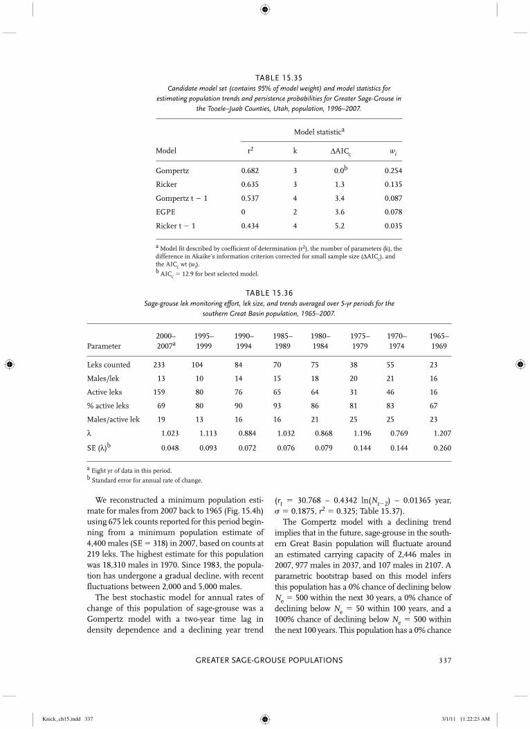
GREATER SAGE-GROUSE POPULATIONS 337
We reconstructed a minimum population esti-mate for males from 2007 back to 1965 (Fig. 15.4h) using 675 lek counts reported for this period begin-ning from a minimum population estimate of 4,400 males (SE � 318) in 2007, based on counts at 219 leks. The highest estimate for this population was 18,310 males in 1970. Since 1983, the popula-tion has undergone a gradual decline, with recent fluctuations between 2,000 and 5,000 males. The best stochastic model for annual rates of change of this population of sage-grouse was a Gompertz model with a two-year time lag indensity dependence and a declining year trend
(rt � 30.768 – 0.4342 ln(Nt�2) – 0.01365 year,� � 0.1875, r2 � 0.325; Table 15.37). The Gompertz model with a declining trend implies that in the future, sage-grouse in the south-ern Great Basin population will fluctuate around an estimated carrying capacity of 2,446 males in 2007, 977 males in 2037, and 107 males in 2107. A parametric bootstrap based on this model infers this population has a 0% chance of declining below Ne � 500 within the next 30 years, a 0% chance of declining below Ne � 50 within 100 years, and a 100% chance of declining below Ne � 500 within the next 100 years. This population has a 0% chance
TABLE 15.35Candidate model set (contains 95% of model weight) and model statistics for
estimating population trends and persistence probabilities for Greater Sage-Grouse in the Tooele–Juab Counties, Utah, population, 1996–2007.
Model statistica
Model r2 k ΔAICc wi
Gompertz 0.682 3 0.0b 0.254
Ricker 0.635 3 1.3 0.135
Gompertz t � 1 0.537 4 3.4 0.087
EGPE 0 2 3.6 0.078
Ricker t � 1 0.434 4 5.2 0.035
a Model fi t described by coeffi cient of determination (r2), the number of parameters (k), the difference in Akaike’s information criterion corrected for small sample size (ΔAICc), and the AICc wt (wi).b AICc � 12.9 for best selected model.
TABLE 15.36Sage-grouse lek monitoring effort, lek size, and trends averaged over 5-yr periods for the
southern Great Basin population, 1965–2007.
Parameter2000– 2007a
1995– 1999
1990– 1994
1985– 1989
1980– 1984
1975– 1979
1970– 1974
1965– 1969
Leks counted 233 104 84 70 75 38 55 23
Males/lek 13 10 14 15 18 20 21 16
Active leks 159 80 76 65 64 31 46 16
% active leks 69 80 90 93 86 81 83 67
Males/active lek 19 13 16 16 21 25 25 23
λ 1.023 1.113 0.884 1.032 0.868 1.196 0.769 1.207
SE (λ)b 0.048 0.093 0.072 0.076 0.079 0.144 0.144 0.260
a Eight yr of data in this period.b Standard error for annual rate of change.
Knick_ch15.indd 337Knick_ch15.indd 337 3/1/11 11:22:23 AM3/1/11 11:22:23 AM

STUDIES IN AVIAN BIOLOGY NO. 38 Knick and Connelly338
of declining below an effective population size of 50 within 30 years across all 26 models of population growth, a 2% chance of declining below Ne � 500 within 30 years, a 4% chance of declining below Ne � 50 within 100 years, and a 78% chance of declin-ing below Ne � 500 within 100 years (Table 15.6).
Comprehensive Analysis of All Leks in the Management Zone
The average number of leks counted per five-year period increased substantially over the assess-ment period (Table 15.38). In 1965–1969, an aver-age of 51 leks per year was censused, but by 2005–2007, an average of 387 leks per year was counted, an increase of 659%. The proportion of active leks decreased over the assessment period, declining from a high of 83% in 1985–1994 to a low of 67% by 2005–2007 (Table 15.38). Popula-tion trends, as indicated by average number of males per lek, decreased over the assessment period by 24%, and average number of males per active lek decreased by 9% (Table 15.38). Average
annual rates of change were 1.0 in three of the eight analysis periods. The average annual rate of change from 1995–1999 to 2000–2007 declined by 10%, but values remained at or above 1.0 for both of these periods (Table 15.38). Starting from a minimum population estimate of 6,851 males (SE � 435) in 2007 based on counts at 471 leks, we reconstructed a minimum popula-tion estimate for males from 2007 back to 1965 (Fig. 15.4i). The population increased from about 6,500 males in 1965 to peak at 14,000 males in 1970, followed by cycles of declines and peaks at 9- to 12-year intervals overlaid on a continuous long-term decline through 2007. The best stochastic model for annual rates of change of the Southern Great Basin SMZ popula-tion of sage-grouse detected a cyclic nature and identified one- or two-year time-delayed Gompertz-type models with declining time trends of �2.6% per year as most representative (e.g., best model with relative likelihood of 28% was rt � 24.334 – 0.391 ln(Nt�1) – 0.010 year � 0.156 period, � � 0.133, r2 � 0.333; Table 15.39).
TABLE 15.37Candidate model set (contains 95% of model weight) and model statistics for
estimating population trends and persistence probabilities for Greater Sage-Grouse in the southern Great Basin population, 1965–2007.
Model statistica
Model r2 k ΔAICc wi
Gompertz t � 2 � year 0.325 5 0.0b 0.462
Gompertz t � 2 � year, period 0.329 6 2.4 0.142
Gompertz t � 1 � year 0.272 5 3.0 0.103
Gompertz t � 2 � period 0.270 5 3.1 0.096
Gompertz t � 1 � period 0.229 5 5.3 0.032
Gompertz t � 1 � year, period 0.275 6 5.5 0.029
Gompertz t � 2 0.164 4 6.1 0.022
Ricker t � 1 � year 0.204 5 6.6 0.017
Gompertz t � 1 0.149 4 6.8 0.015
Ricker t � 2 � year 0.197 5 7.0 0.014
Ricker t � 1 0.140 4 7.2 0.013
Ricker t � 2 0.135 4 7.5 0.011
a Model fi t described by coeffi cient of determination (r2), the number of parameters (k), the difference in Akaike’s information criterion corrected for small sample size (ΔAICc), and the AICc wt (wi).b AICc � –11.3 for best selected model.
Knick_ch15.indd 338Knick_ch15.indd 338 3/1/11 11:22:24 AM3/1/11 11:22:24 AM

TABLE 15.38Sage-grouse lek monitoring effort, lek size, and trends averaged over 5-yr periods for the
Southern Great Basin Management Zone, 1965–2007.
Parameter2000– 2007a
1995– 1999
1990– 1994
1985– 1989
1980– 1984
1975– 1979
1970– 1974
1965– 1969
Leks counted 387 190 170 148 146 121 131 51
Males/lek 13 11 14 16 17 19 20 17
Active leks 257 136 142 123 114 98 103 39
% active leks 67 73 83 83 78 81 80 74
Males/active lek 20 15 17 20 21 24 25 22
λ 1.029 1.141 0.894 1.031 0.937 1.046 0.851 1.169
SE (λ)b 0.040 0.076 0.064 0.069 0.085 0.084 0.083 0.149
a Eight yr of data in this period.b Standard error for annual rate of change.
TABLE 15.39Candidate model set (contains 95% of model weight) and model statistics for
estimating population trends and persistence probabilities for Greater Sage-Grouse in the Southern Great Basin Management Zone, 1965–2007.
Model statistica
Model r2 k ΔAICc wi
Gompertz t � 1 � year, period 0.333 6 0.0b 0.283
Gompertz t � 2� period 0.326 5 0.4 0.230
Gompertz t � 2 � year, period 0.347 6 1.7 0.119
Gompertz t � 1 � year 0.285 5 2.7 0.072
Gompertz t � 2 0.276 4 3.3 0.056
Ricker t � 2 � period 0.262 5 4.0 0.038
Ricker t � 1 � year, period 0.260 6 4.1 0.036
Gompertz t � 1 � period 0.204 5 4.5 0.029
Gompertz t � 2 � year 0.294 5 4.9 0.025
Ricker t � 1 � year 0.244 5 5.0 0.023
Ricker t � 2 0.236 4 5.4 0.019
Gompertz t � 1 0.185 4 5.5 0.018
Ricker t � 1 � period 0.177 5 5.9 0.015
a Model fi t described by coeffi cient of determination (r2), the number of parameters (k), the difference in Akaike’s information criterion corrected for small sample size (ΔAICc), and the AICc wt (wi).b AICc � �43.5 for best selected model.
Knick_ch15.indd 339Knick_ch15.indd 339 3/1/11 11:22:24 AM3/1/11 11:22:24 AM

STUDIES IN AVIAN BIOLOGY NO. 38 Knick and Connelly340
The one-year delayed Gompertz model with declining time trend and period implies the Southern Great Basin SMZ population of sage-grouse will fluctuate around carrying capac-ities that will decline from 12,165 males attend-ing leks in 2007 to 5,517 attending leks in 2037 and 872 males in 2107 if this trend continues at the same rate in the future. A parametric boot-strap based on the one-year time-delayed Gompertz model with declining time trend and period effect, which has a 28% relative likelihood, infers virtually no chance of the population declining below an effective population size of 50 or 500 within 100 years. Multimodel inference indicated that the probability of extinction is 0% in 30 years and only 6% to 8% (SE � 4.9–5.3%) in 100 years (Table 15.6).
Snake River Plain Management Zone
This SMZ represents sage-grouse populations in parts of Montana, Idaho, Utah, Nevada, and Oregon. Almost all sage-grouse in Idaho occur in this SMZ (Fig. 15.1). Seven of the 11 populations delineated within this management zone had data sufficient for analysis.
Baker, Oregon, Population
This population is in eastern Oregon and is sepa-rated by topography from the northern Great Basin population (Table 15.1). Routine monitoring did not
start until the mid- to late 1980s (Table 15.40). The average number of leks counted per five-year period increased substantially from 1985–1989 to 2000–2007 (Table 15.40). An average of 1 lek per year was counted in 1985–1989, but by 2005–2007, an aver-age of 15 leks per year was counted. The proportion of active leks increased over the assessment period, although this could be related to the relatively few leks counted when monitoring began (Table 15.40). Popu-lation trends indicated by average number of males per lek increased over the assessment period by 27%, and average number of males per active lek decreased by 14% (Table 15.40). Con-trary to lek size data, rate of change declined by 11.9% from 1995–1999 to 2000–2007, with an average rate of change 1.0 for 2000–2007 (Table 15.40). The minimum population estimate of 137 males in 2007 was based on counts at 13 leks. We reconstructed a minimum population estimate for males from 2007 back to 1993 (Fig. 15.5a) using 40 lek counts reported for this period. The population has generally fluctuated below 200 males during this period. The best stochastic model for the annual rates of change of Baker, Oregon, population of sage-grouse was an Exponential Growth with Process Error (EGPE, rt � �0.00218, � � 0.1838, SE � 0.0510; Table 15.41). The EPGE model implies this population will decline at an annual rate of �0.22% per year. A parametric bootstrap based on this model infers
TABLE 15.40Sage-grouse lek monitoring effort, lek size, and trends averaged over 5-yr periods for the
Baker, Oregon, population, 1965–2007.
Parameter2000– 2007a
1995– 1999
1990– 1994
1985– 1989
1980– 1984
1975– 1979
1970– 1974
1965– 1969
Leks counted 15 10 4 1 0 0 0 0
Males/lek 14 13 11 — — — — —
Active leks 13 8 3 1 0 0 0 0
% active leks 89 75 78 — — — — —
Males/active lek 16 18 14 — — — — —
λ 0.951 1.079 — — — — —
SE (λ)b 0.126 0.214 — — — — —
a Eight yr of data in this period.b Standard error for annual rate of change.
Knick_ch15.indd 340Knick_ch15.indd 340 3/1/11 11:22:24 AM3/1/11 11:22:24 AM
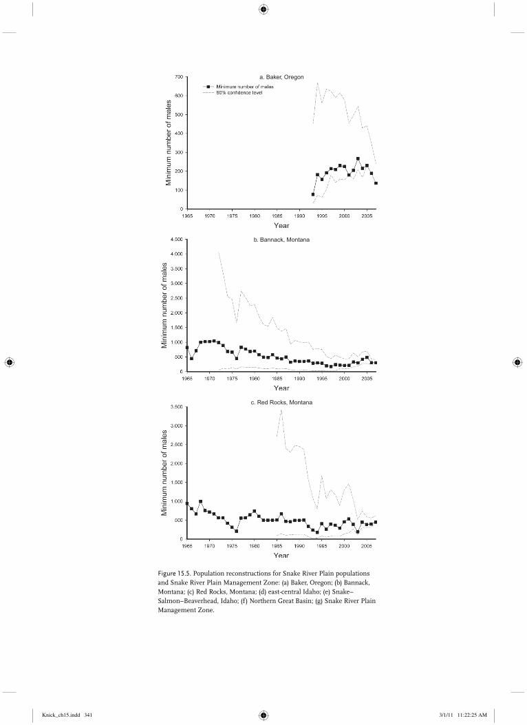
b. Bannack, Montana
c. Red Rocks, Montana
a. Baker, Oregon
Figure 15.5. Population reconstructions for Snake River Plain populations and Snake River Plain Management Zone: (a) Baker, Oregon; (b) Bannack, Montana; (c) Red Rocks, Montana; (d) east-central Idaho; (e) Snake–Salmon–Beaverhead, Idaho; (f) Northern Great Basin; (g) Snake River Plain Management Zone.
Knick_ch15.indd 341Knick_ch15.indd 341 3/1/11 11:22:25 AM3/1/11 11:22:25 AM
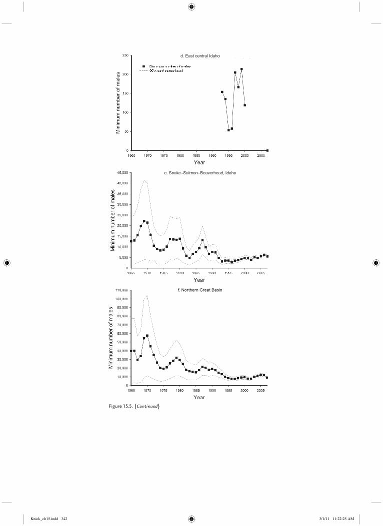
e. Snake–Salmon–Beaverhead, Idaho
f. Northern Great Basin
d. East central Idaho
Figure 15.5. (Continued)
Knick_ch15.indd 342Knick_ch15.indd 342 3/1/11 11:22:25 AM3/1/11 11:22:25 AM

GREATER SAGE-GROUSE POPULATIONS 343
this population has an 8% chance of declining below Ne � 50 and a 100% chance of declining below 500 within the next 30 years. There is a 62% chance, across all 9 models of population growth, of this population declining below an Ne � 50 within 30 yr; a 100% chance of declining below 500 within 30 yr; and a 67% chance of declining below 50 within 100 yr (Table 15.41).
Bannack, Montana, Population
The Bannack, Montana, population is a small population in southwestern Montana separated from nearby populations by distance and moun-tainous terrain (Table 15.1). The average number of leks counted per five-year period was relatively stable through most of the analysis period but
TABLE 15.41Candidate model set (contains 95% of model weight) and model statistics for
estimating population trends and persistence probabilities for Greater Sage-Grouse in the Baker, Oregon, population, 1985–2007.
Model statistica
Model r2 k ΔAICc wi
EGPE 0.000 3 0.0b 0.361
Ricker 0.278 4 1.9 0.138
Gompertz 0.271 3 2.0 0.131
Gompertz t � 1 0.183 4 3.4 0.066
Ricker t � 1 0.160 4 3.7 0.056
Ricker � year 0.418 5 4.0 0.050
Gompertz � year 0.410 5 4.2 0.045
Gompertz t � 2 0.123 4 4.2 0.040
Ricker t � 2 0.112 4 4.4 0.018
a Model fi t described by coeffi cient of determination (r2), the number of parameters (k), the difference in Akaike’s information criterion corrected for small sample size (ΔAICc), and the AICc wt (wi).b AICc � �2.0 for best selected model.
g. Snake River Plain Management Zone
Figure 15.5. (Continued)
Knick_ch15.indd 343Knick_ch15.indd 343 3/1/11 11:22:27 AM3/1/11 11:22:27 AM

STUDIES IN AVIAN BIOLOGY NO. 38 Knick and Connelly344
increased substantially from 1995–1999 to 2000–2007 (Table 15.42). The proportion of active leks declined somewhat over the assessment period, although this could be because only two leks were counted when monitoring began (Table 15.42). Population trends, as indicated by average number of males per lek, declined from a high of 40 males/lek during 1975–1979 to 14 during 2000–2007, a decrease of 65%. Similarly, average number of males per active lek decreased by 58% (Table 15.42). Average rates of change were 1.0 for five of the eight analysis periods but, contrary to lek size data, rates of change increased by 13.6% from the 1995–1999 analysis period to the 2000–2007 period, and rate of change remained at or above 1.0 for the last period (Table 15.42). From a minimum population estimate of 304 males (SE � 65) in 2007 based on counts at 24 leks, we reconstructed a minimum popula-tion estimate for males from 2007 back to 1965 (Fig. 15.5b), using 34 lek counts reported for this period. Less than two leks were counted prior to 1972, which was too few to construct valid confidence intervals. The best stochastic model for the annual rates of change of this population was a Gompertz model with no time lag in density dependence and a period effect (rt � 1.8192 � 0.3233 ln(Nt) � 0.2788 period, � � 0.2015, r2 � 0.175; Table 15.43). The Gompertz model implies that in the future, sage-grouse in the Bannack, Montana,
population will fluctuate around an estimated carrying capacity of 278 males. A parametric bootstrap based on this model infers that this population has a 0% chance of declining below Ne � 50 within the next 30 years, an 86% chance of declining below Ne � 50 within 100 years, and a 99.9% chance of declining below Ne � 500 within the next 100 years. This population has a 6% chance of declining below an effective popu-lation size of 50 within 30 years based on multimodel projections across all 26 models of population growth, a 70% chance of declining below Ne � 500 within 30 years, a 33% chance of declining below Ne � 50 within 100 years, and a 98% chance of declining below Ne � 500 within 100 years (Table 15.6).
Red Rocks, Montana, Population
This population occurs in southwestern Montana just north of the Idaho border and is separated from adjacent populations by distance and moun-tainous terrain (Table 15.1). Few data were availa-ble for analysis until the mid-1980s. The average number of leks counted per five-year period from 1980–1984 to 2000–2007 increased by 1,900% (Table 15.44). The proportion of active leks declined slightly from 1985–1989 to 2000–2007 (Table 15.44). Population trends, as indicated by average number of males per lek, declined sub-stantially from 1980–1984 to 2000–2007, but in part this is likely due to the low number of leks
TABLE 15.42Sage-grouse lek monitoring effort, lek size, and trends averaged over 5-yr periods for the
Bannack, Montana, population, 1965–2007.
Parameter2000– 2007a
1995– 1999
1990– 1994
1985– 1989
1980– 1984
1975– 1979
1970– 1974
1965– 1969
Leks counted 15 3 2 4 4 4 2 2
Males/lek 14 13 19 23 30 40 29 18
Active leks 13 3 2 4 4 4 2 2
% active leks 81 98 100 100 100 100 100 100
Males/active lek 17 14 19 23 30 40 29 18
λ 1.093 0.962 0.969 0.963 0.932 1.072 0.921 1.114
SE (λ)b 0.201 0.229 0.172 0.142 0.078 0.176 0.220 0.084
a Eight yr of data in this period.b Standard error for annual rate of change.
Knick_ch15.indd 344Knick_ch15.indd 344 3/1/11 11:22:28 AM3/1/11 11:22:28 AM

GREATER SAGE-GROUSE POPULATIONS 345
surveyed from 1965–1969 through 1980–1984. Average number of males per active lek followed a similar pattern over the same period (Table 15.44). Average rates of change were 1.0 for three of the eight analysis periods, and generally indicated a sta-ble to increasing population during 1995–1999 and 2000–2007 (Table 15.44). From a minimum population estimate of 448 males (SE � 103) in 2007 based on counts at 30 leks, we reconstructed a minimum popula-tion estimate for males from 2007 back to 1965 (Fig. 15.5c), using 39 lek counts reported for this period. However, too few leks were counted prior
to 1985 to calculate valid confidence intervals. The population has generally fluctuated around 500 males. The best stochastic model for annual rates of change of Red Rocks, Montana, population of sage-grouse was a Gompertz model with a period effect (rt � 3.596 – 0.6089 ln(Nt) � 0.2348 period, � � 0.2925, r2 � 0.307; Table 15.45). The Gompertz model implies this population will fluctuate around an estimated carrying capac-ity of 367 males. A parametric bootstrap based on this model infers that this population has a 0% chance of declining below Ne � 50 within the next
TABLE 15.43Candidate model set (contains 95% of model weight) and model statistics for
estimating population trends and persistence probabilities for Greater Sage-Grouse in the Bannack, Montana, population, 1965–2007.
Model statistica
Model r2 k ΔAICc wi
Gompertz � period 0.175 4 0.0b 0.209
Gompertz � year 0.172 4 0.2 0.192
Gompertz � year, period 0.210 5 0.9 0.133
Ricker � year 0.118 4 2.7 0.054
EGPE 0.000 3 2.9 0.049
Gompertz 0.050 3 3.2 0.043
Ricker � period 0.104 4 3.3 0.040
Ricker 0.034 3 3.8 0.031
Gompertz t � 1 � period 0.090 5 3.9 0.029
Gompertz t � 1 0.026 4 4.2 0.026
Ricker t � 1 0.020 4 4.4 0.023
Gompertz t � 1 � year 0.072 5 4.7 0.020
Ricker � year, period 0.131 5 4.7 0.020
Gompertz t � 2 0.008 4 4.9 0.018
Ricker t � 2 0.008 4 4.9 0.018
Ricker t � 1 � period 0.063 5 5.1 0.016
Period 0.000 3 5.2 0.015
Ricker t � 1 � year 0.054 5 5.5 0.014
Gompertz t � 1 � year, period 0.097 6 6.3 0.009
a Model fi t described by coeffi cient of determination (r2), the number of parameters (k), the difference in Akaike’s information criterion corrected for small sample size (ΔAICc), and the AICc wt (wi).b AICc � �5.5 for best selected model.
Knick_ch15.indd 345Knick_ch15.indd 345 3/1/11 11:22:29 AM3/1/11 11:22:29 AM

STUDIES IN AVIAN BIOLOGY NO. 38 Knick and Connelly346
100 years, a 56.8% chance of declining below Ne � 500 within the next 30 years, and a 94.2% chance of declining below Ne � 500 within 100 years. There is a 0.1% chance, across all 26 models of population growth, of this population declining below Ne � 50 within 30 years, a 55% chance of declining below Ne � 500 within 30 years, a 2.5% chance of declining below Ne � 50 within 100 years, and a 92% chance of declining below Ne � 500 within 100 years (Table 15.6).
Wisdom, Montana, Population
This small, isolated population occurs in south-western Montana and is separated from other pop-ulations by distance and mountainous terrain (Table 15.1). Data are only available for the 2000–2007 analysis period (Table 15.46). Estimates of rates of change were based on an average of six leks counted during this period, and the average rate of change was 1.0 for the 2000–2007 period.
TABLE 15.44Sage-grouse lek monitoring effort, lek size, and trends averaged over 5-yr periods for the
Red Rocks, Montana, population, 1965–2007.
Parameter2000– 2007a
1995– 1999
1990– 1994
1985– 1989
1980– 1984
1975– 1979
1970– 1974
1965– 1969
Leks counted 20 5 4 4 1 1 1 1
Males/lek 13 15 18 31 71 57 73 104
Active leks 15 4 3 4 1 1 1 1
% active leks 75 76 79 100 100 100 100 100
Males/active lek 18 20 21 31 71 57 73 104
λ 1.105 1.088 1.088 1.016 0.932 1.326 0.854 0.977
SE (λ)b 0.282 0.360 0.224 0.169 — — — —
a Eight yr of data in this period.b Standard error for annual rate of change.
TABLE 15.45Candidate model set (contains 95% of model weight) and model statistics for
estimating population trends and persistence probabilities for Greater Sage-Grouse in the Red Rocks, Montana, population, 1965–2007.
Model statistica
Model r2 k ΔAICc wi
Gompertz � period 0.307 4 0.0b 0.382
Gompertz � year 0.295 4 0.7 0.273
Gompertz 0.228 3 1.8 0.152
Gompertz � year, period 0.310 5 2.5 0.112
Ricker � period 0.201 4 5.7 0.022
Ricker � year 0.197 4 5.9 0.020
a Model fi t described by coeffi cient of determination (r2), the number of parameters (k), the difference in Akaike’s information criterion corrected for small sample size (ΔAICc), and the AICc wt (wi).b AICc � 24.3 for best selected model.
Knick_ch15.indd 346Knick_ch15.indd 346 3/1/11 11:22:29 AM3/1/11 11:22:29 AM
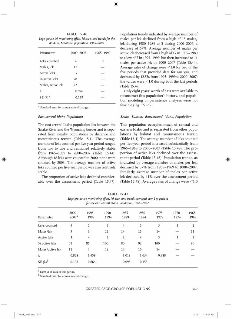
GREATER SAGE-GROUSE POPULATIONS 347
East central Idaho Population
The east central Idaho population lies between the Snake River and the Wyoming border and is sepa-rated from nearby populations by distance and mountainous terrain (Table 15.1). The average number of leks counted per five-year period ranged from two to five and remained relatively stable from 1965–1969 to 2000–2007 (Table 15.44). Although 18 leks were counted in 2000, none were counted by 2003. The average number of active leks counted per five-year period was also relatively stable. The proportion of active leks declined consider-ably over the assessment period (Table 15.47).
Population trends indicated by average number of males per lek declined from a high of 15 males/lek during 1980–1984 to 5 during 2000–2007, a decrease of 67%. Average number of males per active lek decreased from a high of 17 in 1985–1989 to a low of 7 in 1995–1999, but then increased to 11 males per active lek by 2000–2007 (Table 15.44). Average rates of change were 1.0 for two of the five periods that provided data for analysis, and decreased by 42.5% from 1995–1999 to 2000–2007; the values were 1.0 during both the last periods (Table 15.47). Only eight years’ worth of data were available to reconstruct this population’s history, and popula-tion modeling or persistence analyses were not feasible (Fig. 15.5d).
Snake–Salmon–Beaverhead, Idaho, Population
This population occupies much of central and eastern Idaho and is separated from other popu-lations by habitat and mountainous terrain (Table 15.1). The average number of leks counted per five-year period increased substantially from 1965–1969 to 2000–2007 (Table 15.48). The pro-portion of active leks declined over the assess-ment period (Table 15.48). Population trends, as indicated by average number of males per lek, declined by 57% from 1965–1969 to 2000–2007. Similarly, average number of males per active lek declined by 41% over the assessment period (Table 15.48). Average rates of change were 1.0
TABLE 15.46Sage-grouse lek monitoring effort, lek size, and trends for the
Wisdom, Montana, population, 1965–2007.
Parameter 2000–2007 1965–1999
Leks counted 6 0
Males/lek 17 —
Active leks 5 —
% active leks 78 —
Males/active lek 22 —
λ 0.926 —
SE (λ)a 0.169 —
a Standard error for annual rate of change.
TABLE 15.47Sage-grouse lek monitoring effort, lek size, and trends averaged over 5-yr periods
for the east central Idaho population, 1965–2007.
Parameter2000– 2007a
1995– 1999
1990– 1994
1985– 1989
1980– 1984
1975– 1979
1970– 1974
1965– 1969
Leks counted 4 5 3 4 5 3 3 2
Males/lek 5 6 12 14 15 14 — 11
Active leks 3 4 3 3 4 3 3 2
% active leks 51 86 100 80 92 100 — 80
Males/active lek 11 7 12 17 16 14 — —
λ 0.838 1.458 1.018 1.034 0.988 — —
SE (λ)b 0.198 0.864 0.093 0.153 — — —
a Eight yr of data in this period.b Standard error for annual rate of change.
Knick_ch15.indd 347Knick_ch15.indd 347 3/1/11 11:22:29 AM3/1/11 11:22:29 AM

STUDIES IN AVIAN BIOLOGY NO. 38 Knick and Connelly348
for three of the eight analysis periods and declined by 55% between the last two analysis periods, but values remained at or above 1.0 for both of these periods (Table 15.48). The minimum population estimate of 5,457 males (SE � 397) in 2007 was based on counts at 340 leks. We reconstructed a minimum popula-tion estimate for males from 2007 back to 1965 (Fig. 15.5e), using 964 lek counts reported for this period. There was a general decrease in males attending leks in this population through 1992 following a high estimated population count of just over 22,000 in 1969. The population appears to be fluctuating at around 5,000 males since 1992, with an approximate eight-year cycle in population abundance from 1965–1990. The best stochastic model for the annual rates of change of this population was a Gompertz model with a one-year time lag in density depend-ence and a period effect (rt � 2.757 – 0.3281 ln(Nt�1) � 0.2616 × period, � � 0.1856, r2 � 0.351; Table 15.49). The Gompertz model implies sage-grouse in the Snake–Salmon–Beaverhead, Idaho, population will fluctuate around an esti-mated carrying capacity of 4,468 males. A para-metric bootstrap based on this model infers that this population has a 0% chance of declining below Ne � 500 within the next 100 years. Across all 26 models of population growth, there is a 4% chance of this population declining below Ne � 50 within 30 years, a 10% chance of declining below Ne � 500 within 30 years, a 19% chance of
declining below Ne � 50 within 100 years, and a 27% chance of declining below Ne � 500 within 100 years (Table 15.6).
Northern Great Basin Population
This population occupies portions of Nevada, southeastern Oregon, southwestern Idaho, and northwestern Utah (Table 15.1). The average number of leks counted per five-year period increased from 1965–1969 to 2000–2007 (Table 15.50). The proportion of active leks decreased during the assessment period (Table 15.50). Population trends, as indicated by average number of males per lek, declined by 37% from 1965–1969 to 2000–2007. Average number of males per active lek followed the same pattern over the assessment period and declined by 17% (Table 15.50). Average rates of change were 1.0 for three of the eight analysis periods (Table 15.50). Average rate of change declined by 2% between the last two analysis periods, but values remained at or above 1.0 for both of these periods. We reconstructed a minimum population esti-mate for males back to 1965 starting from a mini-mum population estimate of 9,114 males (SE � 520) in 2007 based on counts at 952 leks (Fig. 15.5f), using 4,919 counts at 2,037 leks. The pop-ulation increased from about 40,000 males in 1965 to peak at 57,655 males (SE � 28,345) in 1969, followed by a series of declines and peaks at
TABLE 15.48Sage-grouse lek monitoring effort, lek size, and trends averaged over 5-yr periods
for the Snake–Salmon–Beaverhead, Idaho, population, 1965–2007.
Parameter2000– 2007a
1995– 1999
1990– 1994
1985– 1989
1980– 1984
1975– 1979
1970– 1974
1965– 1969
Leks counted 323 234 165 131 187 138 112 76
Males/lek 15 10 13 20 12 25 30 35
Active leks 207 131 103 108 126 123 94 67
% active leks 65 56 63 81 69 87 85 89
Males/active lek 23 17 20 24 17 28 34 39
λ 1.028 1.082 0.883 1.036 0.932 1.107 0.845 1.117
SE (λ)b 0.050 0.071 0.087 0.089 0.088 0.090 0.070 0.089
a Eight yr of data in this period.b Standard error for annual rate of change.
Knick_ch15.indd 348Knick_ch15.indd 348 3/1/11 11:22:29 AM3/1/11 11:22:29 AM

GREATER SAGE-GROUSE POPULATIONS 349
irregular intervals of 8 to 13 years overlaid on a continuous decline through 2007. The best stochastic model for the annual rates of change of the northern Great Basin population of sage-grouse was a Gompertz model with a one-year time lag and a declining time trend of �4.3% per year (rt � 49.971 � 0.4694 ln(Nt�1) � 0.0208 year, � � 0.1245, r2 � 0.466; Table 15.51).
The one-year delayed Gompertz model with declining time trend implies the northern Great Basin population of sage-grouse will fluctuate around an estimated carrying capacity that will decline from 6,770 males attending leks in 2007 to 1,787 attending leks in 2037 and only 80 males in 2107 if this trend continues at the same rate in the future. This model implies the population
TABLE 15.49Candidate model set (contains 95% of model weight) and model statistics for
estimating population trends and persistence probabilities for Greater Sage-Grouse in the Snake–Salmon–Beaverhead, Idaho, population, 1965–2007.
Model statistica
Model r 2 k ΔAICc wi
Gompertz t � 1 � period 0.351 5 0.0b 0.270
Ricker t � 1 � period 0.349 5 0.1 0.252
Gompertz t � 1 � year, period 0.359 6 2.1 0.095
Ricker t � 1 � year 0.314 5 2.2 0.089
Ricker t � 1 � year, period 0.357 6 2.2 0.088
Gompertz t � 1 � year 0.298 5 3.1 0.057
Ricker t � 2 � period 0.299 5 3.1 0.058
Gompertz t � 2 � period 0.273 5 4.5 0.028
Ricker t � 2 � year, period 0.301 6 5.6 0.017
a Model fi t described by coeffi cient of determination (r2), the number of parameters (k), the difference in Akaike’s information criterion corrected for small sample size (ΔAICc), and the AICc wt (wi).b AICc � �12.1 for best selected model.
TABLE 15.50Sage-grouse lek monitoring effort, lek size, and trends averaged over 5-yr periods
for the northern Great Basin population, 1965–2007.
Parameter2000– 2007a
1995– 1999
1990– 1994
1985– 1989
1980– 1984
1975– 1979
1970– 1974
1965– 1969
Leks counted 595 283 150 126 158 91 96 64
Males/lek 12 9 15 16 16 21 18 19
Active leks 366 196 128 94 127 80 72 52
% active leks 63 71 86 75 78 88 78 81
Males/active lek 19 13 18 22 20 24 23 23
λ 1.007 1.029 0.850 1.054 0.881 1.093 0.806 1.111
SE (λ)b 0.040 0.045 0.050 0.084 0.061 0.078 0.064 0.096
a Eight yr of data in this period.b Standard error for annual rate of change.
Knick_ch15.indd 349Knick_ch15.indd 349 3/1/11 11:22:29 AM3/1/11 11:22:29 AM

STUDIES IN AVIAN BIOLOGY NO. 38 Knick and Connelly350
estimate of 9,114 males attending leks in 2007 was 50% higher than the estimated current carry-ing capacity under this model. A parametric boot-strap based on the time-delayed Gompertz model with declining time trend, which has a 68% rela-tive likelihood, infers that there is virtually no chance of the population declining below Ne � 50 in 30 or 100 years but declining below Ne � 500 is likely (100% relative probability) within 100 years. Multimodel forecasts imply this population has less than a 3% chance of declining below Ne � 50 or Ne � 500 in the short term (30 years) but declining below Ne � 500 in 100 years is certain if the carrying capacity continues to decline (Table 15.6).
Comprehensive Analysis of All Leks in the Management Zone
An average of 146 leks per year was censused in 1965–1969, but by 2005–2007, an average of 1,012 leks per year was counted, an increase of 593%. The proportion of active leks decreased over the assessment period, declining from 88% in 1975–1979 to 64% by 2005–2007 (Table 15.52). Popula-tion trends, as indicated by average number of males per lek, decreased over the assessment period by 54%, and average number of males per active lek decreased by 39% (Table 15.52). Average annual rates of change were 1.0 in three of the eight analysis periods. The average annual rate of
TABLE 15.51Candidate model set (contains 95% of model weight) and model statistics for
estimating population trends and persistence probabilities for Greater Sage-Grouse in the northern Great Basin population, 1965–2007.
Model statistica
Model r2 k ΔAICc wi
Gompertz t � 1 � year 0.466 4 0.0b 0.680
Gomperz t � 1 � year, period 0.467 5 2.6 0.189
Gompertz t � 2 � year 0.406 4 4.3 0.079
a Model fi t described by coeffi cient of determination (r2), the number of parameters (k), the difference in Akaike’s information criterion corrected for small sample size (ΔAICc), and the AICc wt (wi).b AICc � 44.0 for best selected model.
TABLE 15.52Sage-grouse lek monitoring effort, lek size, and trends averaged over 5-yr periods
for the Snake River Plain Management Zone, 1965–2007.
Parameter2000– 2007a
1995– 1999
1990– 1994
1985– 1989
1980– 1984
1975– 1979
1970– 1974
1965– 1969
Leks counted 1,012 556 335 278 364 245 222 146
Males/lek 13 10 14 18 14 23 24 28
Active leks 643 356 249 220 271 219 180 125
% active leks 64 64 75 79 73 88 81 86
Males/active lek 20 15 19 23 19 26 29 33
λ 1.007 1.052 0.867 1.023 0.906 1.089 0.831 1.102
SE (λ)b 0.019 0.022 0.022 0.030 0.031 0.028 0.021 0.029
a Eight yr of data in this period.b Standard error for annual rate of change.
Knick_ch15.indd 350Knick_ch15.indd 350 3/1/11 11:22:29 AM3/1/11 11:22:29 AM
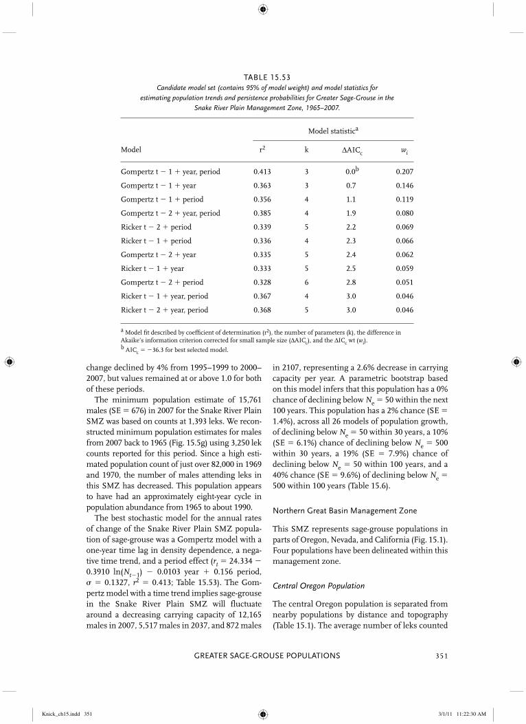
GREATER SAGE-GROUSE POPULATIONS 351
change declined by 4% from 1995–1999 to 2000–2007, but values remained at or above 1.0 for both of these periods. The minimum population estimate of 15,761 males (SE � 676) in 2007 for the Snake River Plain SMZ was based on counts at 1,393 leks. We recon-structed minimum population estimates for males from 2007 back to 1965 (Fig. 15.5g) using 3,250 lek counts reported for this period. Since a high esti-mated population count of just over 82,000 in 1969 and 1970, the number of males attending leks in this SMZ has decreased. This population appears to have had an approximately eight-year cycle in population abundance from 1965 to about 1990. The best stochastic model for the annual rates of change of the Snake River Plain SMZ popula-tion of sage-grouse was a Gompertz model with a one-year time lag in density dependence, a nega-tive time trend, and a period effect (rt � 24.334 � 0.3910 ln(Nt�1) � 0.0103 year � 0.156 period,� � 0.1327, r2 � 0.413; Table 15.53). The Gom-pertz model with a time trend implies sage-grouse in the Snake River Plain SMZ will fluctuate around a decreasing carrying capacity of 12,165 males in 2007, 5,517 males in 2037, and 872 males
in 2107, representing a 2.6% decrease in carrying capacity per year. A parametric bootstrap based on this model infers that this population has a 0% chance of declining below Ne � 50 within the next 100 years. This population has a 2% chance (SE � 1.4%), across all 26 models of population growth, of declining below Ne � 50 within 30 years, a 10% (SE � 6.1%) chance of declining below Ne � 500 within 30 years, a 19% (SE � 7.9%) chance of declining below Ne � 50 within 100 years, and a 40% chance (SE � 9.6%) of declining below Ne � 500 within 100 years (Table 15.6).
Northern Great Basin Management Zone
This SMZ represents sage-grouse populations in parts of Oregon, Nevada, and California (Fig. 15.1). Four populations have been delineated within this management zone.
Central Oregon Population
The central Oregon population is separated from nearby populations by distance and topography (Table 15.1). The average number of leks counted
TABLE 15.53Candidate model set (contains 95% of model weight) and model statistics for
estimating population trends and persistence probabilities for Greater Sage-Grouse in theSnake River Plain Management Zone, 1965–2007.
Model statistica
Model r2 k ΔAICc wi
Gompertz t � 1 � year, period 0.413 3 0.0b 0.207
Gompertz t � 1 � year 0.363 3 0.7 0.146
Gompertz t � 1 � period 0.356 4 1.1 0.119
Gompertz t � 2 � year, period 0.385 4 1.9 0.080
Ricker t � 2 � period 0.339 5 2.2 0.069
Ricker t � 1 � period 0.336 4 2.3 0.066
Gompertz t � 2 � year 0.335 5 2.4 0.062
Ricker t � 1 � year 0.333 5 2.5 0.059
Gompertz t � 2 � period 0.328 6 2.8 0.051
Ricker t � 1 � year, period 0.367 4 3.0 0.046
Ricker t � 2 � year, period 0.368 5 3.0 0.046
a Model fi t described by coeffi cient of determination (r2), the number of parameters (k), the difference in Akaike’s information criterion corrected for small sample size (ΔAICc), and the ΔICc wt (wi).b AICc � �36.3 for best selected model.
Knick_ch15.indd 351Knick_ch15.indd 351 3/1/11 11:22:30 AM3/1/11 11:22:30 AM
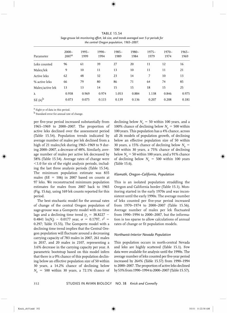
STUDIES IN AVIAN BIOLOGY NO. 38 Knick and Connelly352
per five-year period increased substantially from 1965–1969 to 2000–2007. The proportion of active leks declined over the assessment period (Table 15.54). Population trends indicated by average number of males per lek declined from a high of 21 males/lek during 1965–1969 to 9 dur-ing 2000–2007, a decrease of 48%. Similarly, aver-age number of males per active lek decreased by 58% (Table 15.54). Average rates of change were 1.0 for six of the eight analysis periods, includ-ing the last three analysis periods (Table 15.54). The minimum population estimate was 835 males (SE � 106) in 2007 based on counts at 97 leks. We reconstructed minimum population estimates for males from 2007 back to 1965 (Fig. 15.6a), using 169 lek counts reported for this period. The best stochastic model for the annual rates of change of the central Oregon population of sage-grouse was a Gompertz model with no time lags and a declining time trend (rt � 38.8227 � 0.4841 ln(Nt) � 0.0177 year, � � 0.1797, r2 � 0.297; Table 15.55). The Gompertz model with a declining time trend implies that the Central Ore-gon population will fluctuate around a decreasing carrying capacity of 783 males in 2007, 261 males in 2037, and 20 males in 2107, representing a 3.6% decrease in the carrying capacity per year. A parametric bootstrap based on this model infers that there is a 0% chance of this population declin-ing below an effective population size of 50 within 30 years, a 14.2% chance of declining below Ne � 500 within 30 years, a 72.1% chance of
declining below Ne � 50 within 100 years, and a 100% chance of declining below Ne � 500 within 100 years. This population has a 4% chance, across all 26 models of population growth, of declining below an effective population size of 50 within 30 years, a 15% chance of declining below Ne � 500 within 30 years, a 75% chance of declining below Ne � 50 within 100 years, and a 91% chance of declining below Ne � 500 within 100 years
(Table 15.6).
Klamath, Oregon–California, Population
This is an isolated population straddling the Oregon and California border (Table 15.1). Mon-itoring started in the early 1970s and was incon-sistent until the early 1990s. The average number of leks counted per five-year period increased from 1970–1974 to 2000–2007 (Table 15.56). Average number of males per lek fluctuated from 1990–1994 to 2000–2007, but the informa-tion is too sparse to allow calculations of annual rates of change or fit population models.
Northwest-Interior Nevada Population
This population occurs in north-central Nevada and leks are highly scattered (Table 15.1). Few data were available for analysis until the 1990s. The average number of leks counted per five-year period increased by 264% (Table 15.57) from 1990–1994 to 2000–2007. The proportion of active leks declined by 53% from 1990–1994 to 2000–2007 (Table 15.57).
TABLE 15.54Sage-grouse lek monitoring effort, lek size, and trends averaged over 5-yr periods for
the central Oregon population, 1965–2007.
Parameter2000– 2007a
1995– 1999
1990– 1994
1985– 1989
1980– 1984
1975– 1979
1970– 1974
1965– 1969
Leks counted 96 61 39 27 20 11 12 16
Males/lek 9 10 11 13 10 11 11 21
Active leks 62 48 32 23 14 7 10 13
% active leks 66 79 80 86 71 64 74 85
Males/active lek 13 13 14 15 15 18 15 25
� 0.958 0.969 0.974 1.053 0.884 1.138 0.846 0.975
SE (�)b 0.073 0.075 0.115 0.139 0.136 0.207 0.208 0.181
a Eight yr of data in this period.b Standard error for annual rate of change.
Knick_ch15.indd 352Knick_ch15.indd 352 3/1/11 11:22:30 AM3/1/11 11:22:30 AM

a. Central Oregon
b. Western Great Basin
c. Northern Great Basin Management Zone
Figure 15.6. Population reconstructions for Northern Great Basin popula-tions and Northern Great Basin Management Zone: (a) central Oregon; (b) western Great Basin; (c) Northern Great Basin Management Zone.
Knick_ch15.indd 353Knick_ch15.indd 353 3/1/11 11:22:30 AM3/1/11 11:22:30 AM

STUDIES IN AVIAN BIOLOGY NO. 38 Knick and Connelly354
Population trends, as indicated by average number of males per lek, remained largely unchanged from 1990–1994 to 2000–2007. Average number of males per active lek also remained largely unchanged over the same period (Table 15.57). Average rate of change could only be calculated for the 2000–2007 period and was 1.0 for this period (Table 15.57).
Western Great Basin Population
This population occupies portions of southeast-ern Oregon, northwestern Nevada, and north-eastern California (Table 15.1). The average number of leks counted per five-year period increased considerably from 1965–1969 to 2000–2007 (Table 15.58). The proportion of active leks
TABLE 15.55Candidate model set (contains 95% of model weight) and model statistics for
estimating population trends and persistence probabilities for Greater Sage-Grouse in the central Oregon population, 1965–2007.
Model statistica
Model r2 k �AICc wi
Gompertz � year 0.297 4 0.0b 0.523
Gompertz � year, period 0.323 5 1.2 0.293
Ricker � year 0.199 4 5.3 0.038
Ricker 0.128 3 6.2 0.024
Gompertz 0.119 3 6.6 0.020
Gompertz � period 0.158 4 7.2 0.014
Ricker � year, period 0.211 5 7.3 0.014
Gompertz t � 2 � year 0.148 5 7.7 0.011
Ricker � period 0.148 4 7.7 0.011
Gompertz t � 2 0.071 4 8.7 0.007
a Model fi t described by coeffi cient of determination (r2), the number of parameters (k), the difference in Akaike’s information criterion corrected for small sample size (�AICc), and the AICc wt (wi).b AICc � �14.7 for best selected model.
TABLE 15.56Sage-grouse lek monitoring effort, lek size, and trends averaged over 5-yr periods for
the Klamath, Oregon, population, 1965–2007.
Parameter2000– 2007a
1995– 1999
1990– 1994
1985– 1989
1980– 1984
1975– 1979
1970– 1974
1965– 1969
Leks counted 6 6 5 0 4 2 1 6
Males/lek 4 3 0 — — — — 4
Active leks 1 1 0 — — — — 1
% active leks 58 31 6 — — — — 58
Males/active lek 7 11 3 — — — — 7
� — — — — — — — —
SE (�)b — — — — — — — —
a Eight yr of data in this period.b Standard error for annual rate of change.
Knick_ch15.indd 354Knick_ch15.indd 354 3/1/11 11:22:31 AM3/1/11 11:22:31 AM
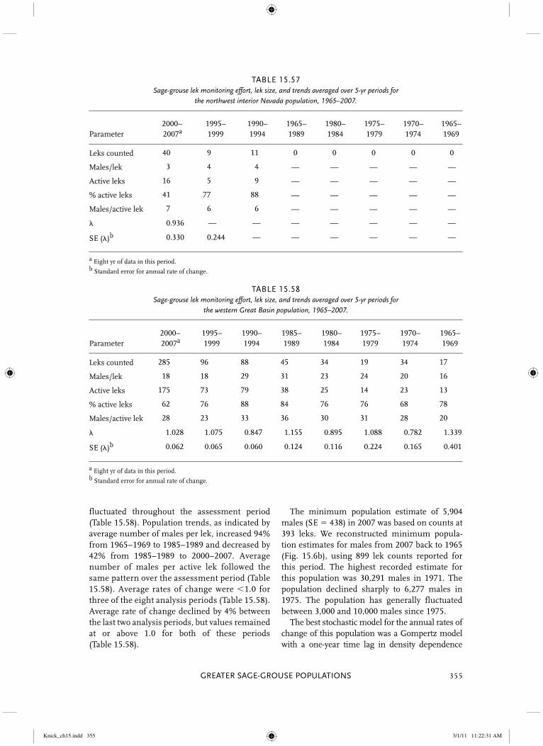
GREATER SAGE-GROUSE POPULATIONS 355
fluctuated throughout the assessment period (Table 15.58). Population trends, as indicated by average number of males per lek, increased 94% from 1965–1969 to 1985–1989 and decreased by 42% from 1985–1989 to 2000–2007. Average number of males per active lek followed the same pattern over the assessment period (Table 15.58). Average rates of change were 1.0 for three of the eight analysis periods (Table 15.58). Average rate of change declined by 4% between the last two analysis periods, but values remained at or above 1.0 for both of these periods (Table 15.58).
The minimum population estimate of 5,904 males (SE � 438) in 2007 was based on counts at 393 leks. We reconstructed minimum popula-tion estimates for males from 2007 back to 1965 (Fig. 15.6b), using 899 lek counts reported for this period. The highest recorded estimate for this population was 30,291 males in 1971. The population declined sharply to 6,277 males in 1975. The population has generally fluctuated between 3,000 and 10,000 males since 1975. The best stochastic model for the annual rates of change of this population was a Gompertz model with a one-year time lag in density dependence
TABLE 15.57Sage-grouse lek monitoring effort, lek size, and trends averaged over 5-yr periods for
the northwest interior Nevada population, 1965–2007.
Parameter2000– 2007a
1995– 1999
1990– 1994
1965– 1989
1980– 1984
1975– 1979
1970– 1974
1965– 1969
Leks counted 40 9 11 0 0 0 0 0
Males/lek 3 4 4 — — — — —
Active leks 16 5 9 — — — — —
% active leks 41 77 88 — — — — —
Males/active lek 7 6 6 — — — — —
� 0.936 — — — — — — —
SE (�)b 0.330 0.244 — — — — — —
a Eight yr of data in this period.b Standard error for annual rate of change.
TABLE 15.58Sage-grouse lek monitoring effort, lek size, and trends averaged over 5-yr periods for
the western Great Basin population, 1965–2007.
Parameter2000– 2007a
1995– 1999
1990– 1994
1985– 1989
1980– 1984
1975– 1979
1970– 1974
1965– 1969
Leks counted 285 96 88 45 34 19 34 17
Males/lek 18 18 29 31 23 24 20 16
Active leks 175 73 79 38 25 14 23 13
% active leks 62 76 88 84 76 76 68 78
Males/active lek 28 23 33 36 30 31 28 20
� 1.028 1.075 0.847 1.155 0.895 1.088 0.782 1.339
SE (�)b 0.062 0.065 0.060 0.124 0.116 0.224 0.165 0.401
a Eight yr of data in this period.b Standard error for annual rate of change.
Knick_ch15.indd 355Knick_ch15.indd 355 3/1/11 11:22:31 AM3/1/11 11:22:31 AM

STUDIES IN AVIAN BIOLOGY NO. 38 Knick and Connelly356
and a declining year trend (rt � 32.6172 � 0.4682 ln(Nt�1) � 0.0143 year, � � 0.1943, r2 � 0.498; Table 15.59). The Gompertz model with a declining trend implies the sage-grouse in the Western Great Basin population will fluctuate around an estimated carrying capacity of 4,111 males in 2007, 1,695 males in 2037, and 200 males in 2107. A parametric bootstrap based on this model infers this popula-tion has a 0% chance of declining below Ne � 500 within the next 30 years, a 0% chance of declining below Ne � 50 within 100 years, and a 100% chance of declining below Ne � 500 within the next 100 years. A multimodel parametric bootstrap predicts that this population has a 5.5% chance of declining below Ne � 50 within 30 years, a 6% chance of
declining below Ne � 500 within 30 years, a 6% chance of declining below Ne � 50 within 100 years, and a 99% chance of declining below Ne � 500 within 100 years (Table 15.6) across all 26 models of population growth.
Comprehensive Analysis of All Leks in the Management Zone
The average number of leks counted per five-year period increased over the assessment period (Table 15.60). An average of 33 leks per year was censused in 1965–1969, but by 2000–2007, an average of 390 leks per year was counted, an increase of 1,082%. The proportion of active leks
TABLE 15.59Candidate model set (contains 95% of model weight) and model statistics for
estimating population trends and persistence probabilities for Greater Sage-Grouse in the western Great Basin population, 1965–2007.
Model statistica
Model r2 k �AICc wi
Gompertz t � 1 � year 0.498 5 0.0b 0.620
Gompertz t � 1 � year, period 0.512 6 1.5 0.293
Ricker t � 1 � year 0.422 5 5.6 0.037
a Model fi t described by coeffi cient of determination (r2), the number of parameters (k), the difference in Akaike’s information criterion corrected for small sample size (�AICc), and the AICc wt (wi).b AICc � �8.4 for best selected model.
TABLE 15.60Sage-grouse lek monitoring effort, lek size, and trends averaged over 5-yr periods for the
Northern Great Basin Management Zone, 1965–2007.
Parameter2000– 2007a
1995– 1999
1990– 1994
1985– 1989
1980– 1984
1975– 1979
1970– 1974
1965– 1969
Leks counted 390 164 134 73 60 33 47 33
Males/lek 15 14 23 24 16 18 17 18
Active leks 240 123 112 63 41 23 33 26
% active leks 63 75 83 85 70 71 70 80
Males/active lek 24 19 27 28 24 25 24 23
� 1.011 1.036 0.874 1.134 0.886 1.092 0.800 0.972
SE (�)b 0.052 0.051 0.054 0.102 0.095 0.156 0.134 0.162
a Eight yr of data in this period.b Standard error for annual rate of change.
Knick_ch15.indd 356Knick_ch15.indd 356 3/1/11 11:22:31 AM3/1/11 11:22:31 AM

GREATER SAGE-GROUSE POPULATIONS 357
decreased over the assessment period, declining from 85% in 1985–1989 to 63% in 2000–2007 (Table 15.60). Population trends, as indicated by average number of males per lek, decreased over the assessment period by 17%, but average number of males per active lek increased by 4% (Table 15.60). Average annual rates of change were 1.0 in four of the eight analysis periods. From 1995–1999 to 2000–2007, average annual rate of change declined by 2%, but values remained at or above 1.0 for both of these periods (Table 15.60). A minimum population estimate of 6,925 males (SE � 464) in 2007 was estimated from counts at 495 leks. We reconstructed minimum population estimates for males from 2007 back to
1965 (Fig. 15.6c) using 1,122 lek counts reported for this period. Since a high estimated population count of 37,915 in 1965, males attending leks have decreased in this SMZ. The best stochastic model for the annual rates of change of the Northern Great Basin SMZ pop-ulation was a Gompertz model with a one-year time lag in density dependence and a negative time trend (rt � 19.157 � 0.2990 ln(Nt�1) � 0.0083 year, � � 0.1683, r2 � 0.240; Table 15.61). The Gompertz model with a time trend implies that sage-grouse in the Northern Great Basin SMZ will fluctuate around a decreasing carrying capacity of 5,529 males in 2007, 2,413 males in 2037, and 349 males in 2107, representing a 2.7%
TABLE 15.61Candidate model set (contains 95% of model weight) and model statistics for
estimating population trends and persistence probabilities for Greater Sage-Grouse in theNorthern Great Basin Management Zone, 1965–2007.
Model statistica
Model r2 k �AICc wi
Gompertz t � 1 � year 0.240 3 0.0b 0.218
Gompertz t � 2 � year 0.221 3 1.0 0.133
Gompertz t � 1 0.157 4 1.7 0.094
Gompertz t � 1 � year, period 0.248 4 2.2 0.072
Gompertz t � 1 � period 0.188 5 2.6 0.058
Gompertz t � 2 0.135 4 2.7 0.056
Ricker t � 1 0.122 5 3.3 0.042
Gompertz t � 2 � year, period 0.223 5 3.5 0.038
Gompertz t � 2 � period 0.171 6 3.5 0.038
Gompertz 0.116 4 3.6 0.036
Ricker t � 2 0.104 5 4.1 0.028
Ricker t � 1 � year 0.157 6 4.2 0.027
Ricker 0.101 5 4.3 0.026
Gompertz � year 0.148 3 4.6 0.022
Ricker t � 1 � period 0.135 3 5.2 0.016
Ricker t � 2 � year 0.135 4 5.2 0.016
Gompertz � period 0.128 4 5.5 0.014
Ricker � year 0.117 5 6.0 0.011
Ricker t � 2 � period 0.117 4 6.0 0.011
a Model fi t described by coeffi cient of determination (r2), the number of parameters (k), the difference in Akaike’s information criterion corrected for small sample size (�AICc), and the AICc wt (wi).b AICc � �19.9 for best selected model.
Knick_ch15.indd 357Knick_ch15.indd 357 3/1/11 11:22:31 AM3/1/11 11:22:31 AM

STUDIES IN AVIAN BIOLOGY NO. 38 Knick and Connelly358
decrease in carrying capacity per year. A paramet-ric bootstrap based on this model infers this pop-ulation has a 0% chance of declining below Ne � 500 within the next 30 years, a 0% chance of declining below Ne � 50 within 100 years, and a 4.7% chance of declining below Ne � 500 within 100 years. There is a 1% chance (SE � 2.0%), across all 26 models of population growth, of this population declining below Ne � 50 within 30 years, a 2% (SE � 2.3%) chance of declining below Ne � 500 within 30 years, a 7% (SE � 5.0%) chance of declining below Ne � 50 within 100 years, and a 29% chance (SE � 8.1%) of declining below Ne � 500 within 100 years (Table 15.6).
Columbia Basin Management Zone
This SMZ represents sage-grouse populations in Washington. Two populations, Moses Cou-lee and Yakima, are delineated within this zone (Fig. 15.1). Genetic diversity in these populations has been lost due to population declines and isolation from core regions of the sage-grouse range (Oyler-McCance and Quinn, this volume, chapter 5).
Moses Coulee, Washington, Population
This population occurs in north-central Washington and is separated from the other Washington population (Yakima) by distance and topography (Table 15.1). The average number of leks counted per five-year period increased from
1965–1969 to 2000–2007 (Table 15.62). The proportion of active leks declined 60% over the assessment period (Table 15.62). Population trends, as indicated by average number of males per lek, declined by 79% from 1965–1969 to 2000–2007. Similarly, average number of males per active lek declined by 50% over the assessment period (Table 15.62). Average rates of change were 1.0 for four of the eight analysis periods. From 1995–1999 to 2000–2007, average rate of change decreased by 4.7%, but values remained at or above 1.0 for both of these periods (Table 15.62). We estimated a minimum population of 230 males (SE � 54) in 2007 based on counts at 32 leks.We reconstructed minimum population estimates for males from 2007 back to 1965 (Fig. 15.7a), using 42 lek counts reported for this period. The highest estimated count was in 1965 with 2,433 males. Since then, the population dramatically declined until about 1993, with population counts fluctuat-ing around 220 males between 1994 and 2007. The best stochastic model for the annual rates of change of this population was a Gompertz model with a one-year time lag and a declining time trend of �4.3% per year (rt � 34.7636 � 0.3689 ln(Nt�1) � 0.01637 year, � � 0.2789, r2 � 0.194; Table 15.63). The Gompertz model with a declining time trend implies that in the future, the Moses Coulee, Washington, population will fluctuate around an estimated carrying capacity that will decline from 168 males attending leks in 2007 to 44 in 2037 and only 2 in 2107. A parametric bootstrap based
TABLE 15.62Sage-grouse lek monitoring effort, lek size, and trends averaged over 5-yr periods for
the Moses Coulee, Washington, population, 1965–2007.
Parameter2000– 2007a
1995– 1999
1990– 1994
1985– 1989
1980– 1984
1975– 1979
1970– 1974
1965– 1969
Leks counted 33 24 19 16 15 14 13 3
Males/lek 7 10 12 13 21 13 27 34
Active leks 12 12 11 10 13 11 12 3
% active leks 38 48 60 66 89 88 95 95
Males/active lek 18 20 19 21 24 14 28 36
� 1.002 1.051 0.902 1.327 0.766 1.122 0.811 0.929
SE (�)b 0.124 0.108 0.151 0.241 0.073 0.210 0.124 0.343
a Eight yr of data in this period.b Standard error for annual rate of change.
Knick_ch15.indd 358Knick_ch15.indd 358 3/1/11 11:22:32 AM3/1/11 11:22:32 AM

a. Moses Coules, Washington
b. Yakima, Washington
c. Columbia Basin Management Zone
Figure 15.7. Population reconstructions for Columbia Basin populations and Columbia Basin Management Zone: (a) Moses-Coulee, Washington; (b) Yakima, Washington; (c) Columbia Basin Management Zone.
Knick_ch15.indd 359Knick_ch15.indd 359 3/1/11 11:22:32 AM3/1/11 11:22:32 AM

STUDIES IN AVIAN BIOLOGY NO. 38 Knick and Connelly360
TABLE 15.63Candidate model set (contains 95% of model weight) and model statistics for
estimating population trends and persistence probabilities for Greater Sage-Grouse in the Moses Coulee, Washington, population, 1965–2007.
Model statistica
Model r2 k �AICc wi
Gompertz t � 1 � year 0.194 5 0.0b 0.207
Gompertz � year 0.192 4 0.1 0.197
Gompertz � year, period 0.213 5 1.7 0.090
Gompertz t � 1 � year, period 0.201 6 2.2 0.067
Gompertz 0.087 3 2.5 0.059
Gompertz t � 1 0.085 4 2.6 0.056
Gompertz t � 2 � year 0.132 5 3.0 0.047
Gompertz t � 1 � period 0.118 5 3.6 0.034
Gompertz t � 2 0.059 4 3.7 0.032
EGPE 0.000 3 3.8 0.031
Gompertz � period 0.112 4 3.9 0.030
Ricker 0.041 3 4.5 0.022
Gompertz t � 2 � period 0.092 5 4.8 0.019
Ricker t � 1 0.033 4 4.8 0.019
Ricker t � 2 0.024 4 5.2 0.016
Gompertz t � 2 � year, period 0.132 6 5.6 0.013
Ricker � year 0.072 4 5.7 0.012
a Model fi t described by coeffi cient of determination (r2), the number of parameters (k), the difference in Akaike’s information criterion corrected for small sample size (�AICc), and the AICc wt (wi).b AICc � 20.5 for best selected model.
on this model infers a 9% chance of this popula-tion declining below Ne � 50 within 30 years, a 100% chance of this population declining below Ne � 50 within 100 years, and a 100% chance of declining below Ne � 500 within 30 years. Across all 26 models of population growth, this popula-tion has a 10% chance of declining below Ne � 50 within 30 years, an 88% chance of declining below Ne � 500 within 30 years, a 62% chance of declin-ing below Ne � 50 within 100 years, and a 99.8% chance of declining below Ne � 500 within 100 years (Table 15.6).
Yakima, Washington, Population
This population occurs in south-central Washington and is separated from other populations by dis-
tance and the Columbia River (Table 15.1). The average number of leks counted per five-year period increased from 1970–1974 to 2000–2007 (Table 15.64). An average of 1 lek per five-year period was censused in 1970–1974, but by 2005–2007, an average of 10 leks was counted. The pro-portion of active leks declined over the assessment period (Table 15.64). Population trends, as indi-cated by average number of males per lek, increased 300% from 1975–1979 to 1980–1984 but declined by 73% from 1980–1984 to 2000–2007. However, relatively few leks existed to count throughout the assessment period. Average number of males per active lek also showed the same pattern over the assessment period (Table 15.64). Average rates of change were 1.0 for four of the eight analysis periods. Average rate of change declined by 12%
Knick_ch15.indd 360Knick_ch15.indd 360 3/1/11 11:22:33 AM3/1/11 11:22:33 AM

GREATER SAGE-GROUSE POPULATIONS 361
TABLE 15.64Sage-grouse lek monitoring effort, lek size, and trends averaged over 5-yr periods for
the Yakima, Washington, population, 1965–2007.
Parameter2000– 2007a
1995– 1999
1990– 1994
1985– 1989
1980– 1984
1975– 1979
1970– 1974
1965– 1969
Leks counted 10 7 5 4 3 2 1 0
Males/lek 13 16 23 29 48 19 12 —
Active leks 8 6 5 4 3 2 1 —
% active leks 81 89 93 87 97 100 100 —
Males/active lek 16 18 26 34 49 19 12 —
� 0.939 1.065 0.939 0.905 1.071 1.408 0.752 —
SE (�)b 0.110 0.158 0.107 0.238 0.080 0.151 — —
a Eight yr of data in this period.b Standard error for annual rate of change.
between the last two analysis periods and was 1.0 during 2000–2007 (Table 15.64). The minimum population estimate was 85 males (SE � 24) in 2007 based on counts at seven leks. We reconstructed minimum population estimates for males from 2007 back to 1970 (Fig. 15.7b), using 24 lek counts reported for this period. Because only one lek was surveyed from 1970–1974, confidence intervals on the population estimate could only be calculated to 1975. The population increased from 396 in 1970 to peak at 779 in 1983, followed by a decline through 2007. The best stochastic model for the annual rates of change of this population was a Gompertz model with a two-year time lag and no period effects or time trend (rt � 0.8762 – 0.1667 ln(Nt�2),� � 0.2934, r2 � 0.085; Table 15.65). Based on this model, the estimated carrying capacity for this pop-ulation was 192 males. A parametric bootstrap based on this model infers this population has a 0.4% and 1.6% chance of declining below Ne � 50 within 30 and 100 years, respectively. The population is now below Ne � 500 and has a 26% chance, across all 26 models of population growth, of declining below Ne � 50 within 30 years and a 50% chance of declin-ing below Ne � 50 within 100 years (Table 15.6).
Comprehensive Analysis of All Leks in the Management Zone
The average number of leks counted per five-year period increased over the assessment
period (Table 15.65). An average of 3 leks per year was censused in 1965–1969, but by 2005–2007, an average of 42 leks per year was counted, an increase of 1,300%. The proportion of active leks decreased over the assessment period, averaging between 92% and 100% from 1965 to 1984 but decreased to 47% by 2000–2007 (Table 15.66). Population trends, as indicated by aver-age number of males per lek and average number of males per active lek, also decreased over the assessment period by 76 and 53%, respectively (Table 15.66). Average annual rates of change were 1.0 in five of the eight analysis periods. The average annual rate of change from the 1995–1999 to 2000–2007 declined by 6.5% and the value was 1.0 for the last period (Table 15.66). A minimum population estimate of 315 males (SE � 59) in 2007 was estimated from counts at 39 leks. We reconstructed minimum population estimates for males from 2007 back to 1965 (Fig. 15.7c) using 64 lek counts reported for this period. Because only one lek was surveyed in 1965 and 1966, confidence intervals on the pop-ulation estimate could only be calculated to 1975. The number of males attending leks in this SMZ has decreased since an estimated high of 2,665 in 1965. The best stochastic model for the annual rates of change in the Columbia Basin SMZ sage-grouse population was a Gompertz model with no time lag and a negative time trend (rt � 28.817 � 0.3842
Knick_ch15.indd 361Knick_ch15.indd 361 3/1/11 11:22:33 AM3/1/11 11:22:33 AM

STUDIES IN AVIAN BIOLOGY NO. 38 Knick and Connelly362
ln(Nt) � 0.0133 × year, � � 0.211, r2 � 0.193; Table 15.67). The Gompertz model with a time trend implies sage-grouse in the Columbia Basin SMZ will fluctuate around a decreasing carrying capacity of 192 males in 2007, 103 males in 2037, and nine males in 2107. A parametric bootstrap based on this model infers that this population has a 0% chance of declining below Ne � 50 within the next 30 years, a 100% chance of declining below Ne � 50 within 100 years. This population has a 12% (SE � 6.0%) chance across all 26 models
of population growth of declining below Ne � 50 within 30 years, a 62% (SE � 9.1%) chance of declining below 50 within 100 years, a 76% (SE � 6.5%) chance of declining below Ne � 500 within 30 years, and an 86% (SE � 5.8%) of declining below Ne � 500 in 100 years (Table 15.6).
Colorado Plateau Management Zone
This SMZ represents sage-grouse populations in parts of Utah and Colorado. Of the five populations
TABLE 15.65Candidate model set (contains 95% of model weight) and model statistics for
estimating population trends and persistence probabilities for Greater Sage-Grouse in the Yakima, Washington, population, 1965–2007.
Model statistica
Model r2 k �AICc wi
Gompertz t � 2 0.085 4 0.0b 0.106
Ricker t � 2 0.072 4 0.5 0.082
EGPE 0.000 3 0.7 0.074
Gompertz t � 2 � year 0.132 5 0.7 0.073
Gompertz t � 2 � period 0.121 5 1.2 0.059
Gompertz t � 1 0.049 4 1.4 0.053
Ricker t � 2 � year 0.114 5 1.4 0.052
Ricker t � 2 � period 0.114 5 1.4 0.052
Gompertz 0.044 3 1.5 0.049
Ricker 0.040 3 1.7 0.046
Ricker t � 1 0.033 4 1.9 0.040
Ricker � period 0.092 4 2.3 0.034
Gompertz � period 0.089 4 2.4 0.032
Gompertz t � 1 � period 0.086 5 2.5 0.030
Gompertz t � 1 � year 0.086 5 2.5 0.030
Gompertz � year 0.083 4 2.6 0.028
Period 0.015 3 2.6 0.029
Ricker � year 0.076 4 2.9 0.025
Ricker t � 1 � period 0.073 5 3.0 0.023
Ricker t � 1 � year 0.065 5 3.3 0.020
Gompertz t � 2 � year, period 0.132 6 3.5 0.019
a Model fi t described by coeffi cient of determination (r2), the number of parameters (k), the difference in Akaike’s information criterion corrected for small sample size (�AICc), and the AICc wt (wi).b AICc � 20.3 for best selected model.
Knick_ch15.indd 362Knick_ch15.indd 362 3/1/11 11:22:33 AM3/1/11 11:22:33 AM

GREATER SAGE-GROUSE POPULATIONS 363
delineated within this zone, only the Piceance Basin had sufficient data for analysis.
Piceance Basin, Colorado, Population
This population occurs in the Piceance Basin, Colorado and is separated from adjacent popula-tions by distance and topography (Table 15.1). Few data were available for analysis until the 2000–2007 analysis period (Fig. 15.8a). The pro-portion of active leks and lek size was low in 2000–2007 (Table 15.68). Average rate of change could only be calculated for the 2000–2007 period and was �1.0 for this period.
Comprehensive Analysis of All Leks in the Management Zone
The average number of leks counted per five-year period increased over the assessment period (Table 15.69). An average of 2 leks per year was censused in 1965–1969 but by 2005–2007, an average of 37 leks per year was counted, an increase of 1,750%. The proportion of active leks decreased over the assessment period, declining from 84% from 1980–1984 to 45% by 2000–2007 (Table 15.69). Population trends, as indicated by average number of males per lek, decreased from 1980–1984 to 2000–2007, but average number of males per active lek increased by 44% (Table 15.69). Average annual rates of change were 1.0 in three of the four analysis periods. The average
annual rate of change increased by 34% from 1995–1999 to 2000–2007 (Table 15.69). The minimum population estimate of 241 males (SE � 52) in 2007 was based on counts at 73 leks. We reconstructed minimum population estimates for males from 2007 back to 1984 (Fig. 15.8b) using 100 lek counts reported for this period. The best stochastic model for the annual rates of change of the Colorado Plateau SMZ was a Gompertz model with no time lag (rt � 2.788 – 0.5071 Nt, � � 0.1454, r2 � 0.298; Table 15.70) which was matched by a Ricker model with simi-lar performance. The Gompertz model implies that sage-grouse populations in the Colorado Pla-teau SMZ will fluctuate around a carrying capac-ity of 244 males with no change through time. A parametric bootstrap based on this model infers that this SMZ has virtually no chance of declining below Ne � 50 within 30 or 100 years. This popula-tion of grouse in this SMZ has no chance, across all 26 models of population growth, of declining below Ne � 50 within 30 years, a 96% (SE � 3.7%) of declin-ing below Ne � 500 in 30 years, a 5% (SE � 2.3%) chance of declining below Ne � 50 within 100 years, and a 98% (SE � 3.7%) chance of declining below Ne � 500 within 100 years (Table 15.6).
Metapopulation Analysis
Estimated dispersal rates among SMZs were gen-erally low, never exceeding 5% of the SMZ’s abun-dance dispersing to any other SMZ (Table 15.71).
TABLE 15.66Sage-grouse lek monitoring effort, lek size, and trends averaged over 5-yr periods for the
Columbia Basin Management Zone, 1965–2007.
Parameter2000– 2007a
1995– 1999
1990– 1994
1985– 1989
1980– 1984
1975– 1979
1970– 1974
1965– 1969
Leks counted 42 31 24 20 18 16 16 3
Males/lek 8 11 14 16 25 13 24 34
Active leks 20 18 16 14 16 14 13 3
% active leks 47 57 67 70 89 90 90 95
Males/active lek 17 20 20 23 28 15 26 36
� 0.977 1.045 0.891 1.123 0.858 1.185 0.809 0.929
SE (�)b 0.088 0.102 0.110 0.163 0.091 0.170 0.117 —
a Eight yr of data in this period.b Standard error for annual rate of change.
Knick_ch15.indd 363Knick_ch15.indd 363 3/1/11 11:22:33 AM3/1/11 11:22:33 AM

STUDIES IN AVIAN BIOLOGY NO. 38 Knick and Connelly364
Highest estimated dispersal occurred between the Great Plains and Wyoming Basin SMZs, between Snake River Plain and Northern Great Basin SMZs, and between Southern Great Basin and Snake River Plain SMZs with rates of 5%, 3.5%, and 2.4%, respectively. Correlated population dynamics were prevalent among many of the SMZs (Table 15.72). Highest correlations were between Southern Great Basin and Snake River Plain SMZs, between Southern Great Basin and Northern Great Basin SMZs, and between Snake River Plain and Northern Great Basin SMZs, with
correlation coefficients of 0.58, 0.50, and 0.52, respectively. A slight negative correlation (�0.04) was found between Great Plains and Northern Great Basin SMZs. Metapopulation projections were basedon dispersal and correlations among SMZ populations and individual SMZ growth models based on Gompertz and Ricker types of density dependence (Table 15.73). Projections based on the information- theoretic (IT) best Gompertz models, which were also the best models overall, suggested a low probability
TABLE 15.67Candidate model set (contains 95% of model weight) and model statistics for
estimating population trends and persistence probabilities for Greater Sage-Grouse in the Columbia Basin Management Zone, 1965–2007.
Model statistica
Model r2 k �AICc wi
Gompertz � year 0.193 3 0.0b 0.257
Gompertz t � 1 � year 0.160 3 1.6 0.113
Gompertz � year, period 0.201 4 2.2 0.084
Ricker � year 0.137 4 2.7 0.066
Gompertz 0.066 5 3.4 0.047
EGPE 0.000 4 3.8 0.039
Ricker 0.054 5 3.9 0.037
Gompertz t � 1 0.055 5 3.9 0.037
Gompertz t � 1 � year, Period 0.164 6 4.0 0.034
Gompertz � period 0.107 4 4.1 0.034
Gompertz t � 2 � year 0.103 5 4.3 0.031
Ricker t � 1 0.037 6 4.6 0.026
Gompertz t � 2 0.035 5 4.7 0.025
Gompertz t � 1 � period 0.090 3 4.8 0.023
Ricker � year, period 0.143 3 5.0 0.021
Ricker � period 0.081 4 5.2 0.019
Ricker t � 1 � year 0.082 4 5.2 0.020
Ricker t � 2 0.023 5 5.2 0.019
Period 0.001 4 6.1 0.012
Gompertz t � 2 � period 0.061 5 6.1 0.012
a Model fi t described by coeffi cient of determination (r2), the number of parameters (k), the difference in Akaike’s information criterion corrected for small sample size (�AICc), and the AICc wt (wi).b AICc � �1.9 for best selected model.
Knick_ch15.indd 364Knick_ch15.indd 364 3/1/11 11:22:33 AM3/1/11 11:22:33 AM
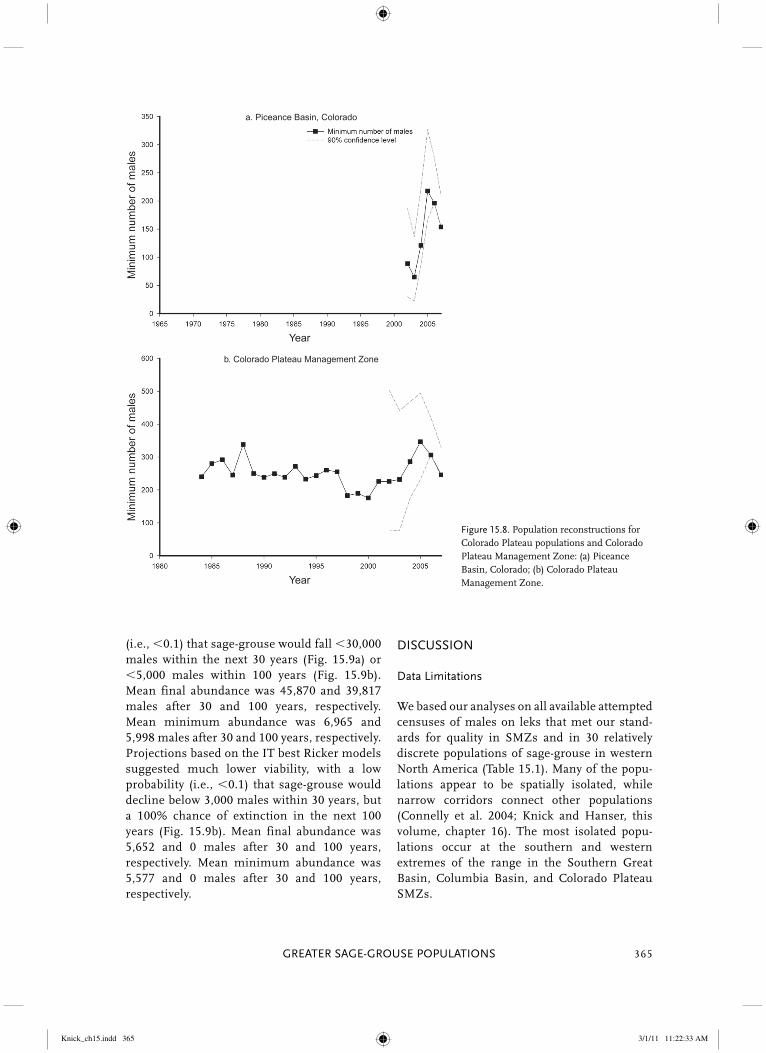
GREATER SAGE-GROUSE POPULATIONS 365
(i.e., 0.1) that sage-grouse would fall 30,000 males within the next 30 years (Fig. 15.9a) or 5,000 males within 100 years (Fig. 15.9b). Mean final abundance was 45,870 and 39,817 males after 30 and 100 years, respectively. Mean minimum abundance was 6,965 and 5,998 males after 30 and 100 years, respectively. Projections based on the IT best Ricker models suggested much lower viability, with a low probability (i.e., 0.1) that sage-grouse would decline below 3,000 males within 30 years, but a 100% chance of extinction in the next 100 years (Fig. 15.9b). Mean final abundance was 5,652 and 0 males after 30 and 100 years, respectively. Mean minimum abundance was 5,577 and 0 males after 30 and 100 years, respectively.
DISCUSSION
Data Limitations
We based our analyses on all available attempted censuses of males on leks that met our stand-ards for quality in SMZs and in 30 relatively discrete populations of sage-grouse in western North America (Table 15.1). Many of the popu-lations appear to be spatially isolated, while narrow corridors connect other populations (Connelly et al. 2004; Knick and Hanser, this volume, chapter 16). The most isolated popu-lations occur at the southern and western extremes of the range in the Southern Great Basin, Columbia Basin, and Colorado Plateau SMZs.
a. Piceance Basin, Colorado
b. Colorado Plateau Management Zone
Year
Year
Figure 15.8. Population reconstructions for Colorado Plateau populations and Colorado Plateau Management Zone: (a) Piceance Basin, Colorado; (b) Colorado Plateau Management Zone.
Knick_ch15.indd 365Knick_ch15.indd 365 3/1/11 11:22:33 AM3/1/11 11:22:33 AM

STUDIES IN AVIAN BIOLOGY NO. 38 Knick and Connelly366
Not all leks are currently active, and many have been inactive for several years. The total number of leks that has been extirpated is unknown and hinders our attempts to fully understand the magnitude of change in sage-grouse populations. Although leks have become inactive throughout the species’ range, the dis-tribution of inactive leks appears to be clustered rather than widespread (Connelly et al. 2004). Proportionally, the largest number of inactive leks appears to occur in the Southern Great Basin, Columbia Basin, and Colorado Plateau
SMZs. Applying a three-stage probability sam-pling approach, described below, in the future would provide unbiased estimates of the pro-portion of leks disappearing and new leks established, as well as facilitate modeling impacts of habitat changes and threat factors on sage-grouse abundance and population dynamics. An examination of all trend data from the mid-1940s to 2003 suggests a substantial decline in the overall sage-grouse population in North America (Connelly et al. 2004). However, because
TABLE 15.68Sage-grouse lek monitoring effort, lek size, and trends averaged over 5-yr periods for the
the Piceance Basin, Colorado, population, 1965–2007.
Parameter2000– 2007a
1995– 1999
1990– 1994
1985– 1989
1980– 1984
1975– 1979
1970– 1974
1965– 1969
Leks counted 28 1 7 13 6 0 0 0
Males/lek 4 — — — — — — —
Active leks 13 — — — — — — —
% active leks 51 — — — — — — —
Males/active lek 8 — — — — — — —
� 1.216 — — — — — — —
SE (�)b 0.229 — — — — — — —
a Eight yr of data in this period.b Standard error for annual rate of change.
TABLE 15.69Sage-grouse lek monitoring effort, lek size, and trends averaged over 5-yr periods for the
Colorado Plateau Management Zone, 1965–2007.
Parameter2000– 2007a
1995– 1999
1990– 1994
1985– 1989
1980– 1984
1975– 1979
1970– 1974
1965– 1969
Leks counted 37 4 12 19 10 2 2 2
Males/lek 6 9 6 9 8 — — 3
Active leks 16 3 4 8 8 1 1 1
% active leks 45 64 54 68 84 — — 63
Males/active lek 13 17 10 12 9 — — —
� 1.063 0.793 0.938 0.991 — — — —
SE (�)b 0.396 — — — — — — —
a Eight yr of data in this period.b Standard error for annual rate of change.
Knick_ch15.indd 366Knick_ch15.indd 366 3/1/11 11:22:34 AM3/1/11 11:22:34 AM

GREATER SAGE-GROUSE POPULATIONS 367
data collected in the 1940s and 1950s are highly variable and may have been collected in a some-what haphazard fashion, they permit no means of assessing the true magnitude of the popula-tion change. Confidence intervals for population reconstructions for all populations and SMZs clearly show that precisions of recent population indices are dramatically smaller than the earlier ones based on smaller samples of leks in the dec-ades from 1960 to 1980.
All states and provinces monitor sage-grouse breeding populations by counting males attend-ing leks during the spring breeding season. Standard techniques for censusing leks have been available for a number of years (Patterson 1952, Eng 1963, Jenni and Hartzler 1978, Emmons and Braun 1984) and were recently summarized (Con-nelly et al. 2003b). Despite available information, methods differ among agencies and even among years within agencies (Connelly et al. 2004). These
TABLE 15.70Candidate model set (contains 95% of model weight) and model statistics in the
estimating population trends and persistence probabilities for Greater Sage-Grouse in the Colorado Plateau Management Zone, 1965–2007.
Model statistica
Model r2 k �AICc wi
Ricker 0.264 4 0.0b 0.313
Gompertz 0.246 4 0.5 0.244
EGPE 0.000 3 1.5 0.148
Ricker � year 0.264 5 3.2 0.063
Gompertz � year 0.000 5 3.7 0.049
Ricker t � 1 0.247 4 4 0.042
Gompertz t � 1 0.108 4 4.1 0.040
Gompertz t � 2 0.103 4 4.3 0.037
Ricker t � 2 0.098 4 4.6 0.031
a Model fi t described by coeffi cient of determination (r2), the number of parameters (k), the difference in Akaike’s information criterion corrected for small sample size (�AICc), and the AICc wt (wi).b AICc � 15.0 for best selected model.
TABLE 15.71Dispersal rates among sage-grouse management zones representing the proportion of the population
dispersing to another management zone each year.
Wyoming
BasinSouthern
Great BasinSnake River
PlainNorthern
Great BasinColorado Plateau
Great Plains 0.050
Wyoming Basin 0.020 0.011 0.009
Southern Great Basin 0.024 0.004 0.005
Snake River Plain 0.035
Connections between management zones not presented are assumed to be zero.
Knick_ch15.indd 367Knick_ch15.indd 367 3/1/11 11:22:34 AM3/1/11 11:22:34 AM

Pro
babi
lity
Pro
babi
lity
a.
b.
Figure 15.9. Greater Sage-Grouse metapopulation probability of persistence at: (a) 30 years and (b) 100 years. N(ext) is population abundance at which species is declared extinct.
inconsistencies confound attempts to make com-parisons of population trends across states and provinces. Nevertheless, long-term lek counts make up the largest range-wide database available for sage-grouse populations and provide the basis for reconstructing a remarkably precise index to minimum male abundance at a relatively broad spatial scale (Connelly et al. 2004). Without efforts to take a probability sample of leks in each spatial region and apply intense methods in local areas to convert this index into a valid estimator of both male and female breeding sage-grouse, data on populations of sage-grouse will face challenges to their validity. Lek counts focus on attendance of males. Some male sage-grouse may not attend a lek or may attend two or more leks (Jenni and Hartzler 1978,
Emmons and Braun 1984, Walsh et al. 2004). Lek data used to track populations have an implied assumption that probability of detection of birds does not change among years (i.e., the proportion missed because of nonattendance or attendance at a lek that is not counted remains about the same) or that it varies randomly. Even if the detec-tion probability is unknown, which is usually the case, the problem can be minimized to more pre-cise counts if leks counted on a single morning are relatively close and represent all or a signifi-cant part of a given local breeding population, a deme. Repeating these counts along a lek route at weekly intervals centered around the peak in male attendance will ensure their reliability and com-parability across regions. Combining these extensive counts with intensive mark-resight or
Knick_ch15.indd 368Knick_ch15.indd 368 3/1/11 11:22:34 AM3/1/11 11:22:34 AM

GREATER SAGE-GROUSE POPULATIONS 369
TABLE 15.72Correlation in model residuals among sage-grouse management zones for the AICc
best Gompertz and Ricker (in parentheses) models.
Great Plains
Wyoming Basin
Southern Great Basin
Snake River Plain
Northern Great Basin
Columbia Basin
Colorado Plateau
Great Plains 1 0.46 (0.46) 0.05 (0.08) 0.41 (0.41) �0.04 (�0.02) 0.31 (0.31) 0.13 (0.09)
Wyoming Basin 1 0.32 (0.35) 0.34 (0.38) 0.09 (0.19) 0.10 (0.17) 0.27 (0.18)
Southern Great Basin 1 0.58 (0.58) 0.50 (0.50) 0.12 (0.14) 0.19 (0.10)
Snake River Plain 1 0.52 (0.57) 0.31 (0.32) 0.22 (0.07)
Northern Great Basin 1 0.36 (0.38) 0.53 (0.42)
Columbia Basin 1 0.03 (0.02)
Colorado Plateau 1
telemetry studies in a few areas would provide better data to verify their reliability as an unbiased index to grouse population abundance. Unfortunately, counting males attending some leks in a region provides little more than an index to the minimum number of males present in a region. We developed an approach to analyzing this index that treats lek counts as a cluster sam-ple of males within leks and applies ratio estimators to paired counts of males at leks in succeeding years to obtain unbiased estimators of �(t), the finite rate of change from the previous year to the present year, and (t), its reciprocal. Population reconstruction using these unbiased estimators provides remarkably precise estimates of the rates of change for reconstructing the index in previous years and is not biased by changes in the number of leks counted in different years. These rates of change are the basis for our mode-ling efforts. Unfortunately, the final year count of males attending leks is not based on a probability sample and cannot be used to infer the true number of males attending leks within the spatial region sampled, the true number of males present within the region, or the breeding population of both males and females present within the spatial region sampled. Methods to replace this weak foundation of lek counts representing an unknown proportion of leks in a spatial region by a true probability sample of leks and breeding males and females in defined spatial areas have been proposed but not widely adopted at this time (Garton et al. 2007).
Analytical Approach and Inference
We had sufficient data on 24 populations and six SMZs to reconstruct populations back to at least 1967. Forty-six percent of these populations peaked in 1969, and 77% peaked from 1969–1972. Fifty percent of these SMZs peaked in 1969. Clearly, our population reconstruction approach demonstrated a pattern of relatively high num-bers of sage-grouse during the late 1960s and early 1970s. Independent data—population data not based on lek counts—could help validate or refute our approach to population reconstruction. Unfortunately, little published information is available on sage-grouse population change that is not based on lek counts, but some information on production and harvest is available. Sage-grouse production in six states, measured by age ratios in the harvest, was considerably higher from the late 1960s to the early 1980s compared to 1986–1996 (Connelly and Braun 1997). Between 1965 and 1979 in Idaho, the average number of chicks per hen peaked in 1969 (Autenrieth 1981). Between 1965 and 1992, sage-grouse production in Oregon peaked in 1969, while total birds counted during summer surveys peaked in 1971 (Willis et al. 1993). Similarly, from 1965 to 1990, chicks per adult, percent adults with broods, and mean brood size in Oregon were greatest in the late 1960s and early 1970s (Drut 1994). Addition-ally, estimated peak harvest occurred in Idaho in 1969 (Autenrieth 1981) and in Oregon and Washington in 1970 (Drut 1994). During the late
Knick_ch15.indd 369Knick_ch15.indd 369 3/1/11 11:22:35 AM3/1/11 11:22:35 AM

STUDIES IN AVIAN BIOLOGY NO. 38 Knick and Connelly370
1960s, Montana substantially increased their season length for sage-grouse (Wallestad 1975a), which presumably was at least in part related to grouse abundance. Thus, several independent sources of data also strongly suggest relatively high populations of sage-grouse in the late 1960s and early 1970s and lend further support to our approach to population reconstruction. Previous suggestions of the possibility of cyclic patterns in abundance of sage-grouse (Rich 1985, Connelly et al. 2004) led us to apply information-theoretic methods to assessment of first-order, second-order, and third-order models of density dependence. Zeng et al. (1998) earlier demon-strated their success in detecting complex pat-terns of density dependence using Schwartz’s information criterion. Our use of AICc led to selection of one-year or two-year time delayed density-dependent models for 33% of the popula-tions and SMZs, but in most cases no single model was selected as the single best model. Therefore, we chose to take a multimodel inferen-tial approach to ensure adequate incorporation of model uncertainty and its implications for forecasting future viability and persistence of the populations. Our findings generally agree with conclusions of other recent analyses (Connelly et al. 2004, Anonymous 2008) that also documented declin-ing sage-grouse populations. However, our multimodel predictions of the likelihood of indi-vidual populations of sage-grouse declining below Ne � 50 (13%, Table 15.6) and Ne � 500 (54%) within 30 years are clearly underestimates of the true percentages because they are based solely on the 24 populations for which we had sufficient data to build stochastic growth models. Many smaller populations could not be analyzed and modeled because of lack of sufficient data. Our analyses suggest that smaller populations have suffered greater declines and tend to be at greater risk than larger populations. Another recent approach to analyzing lek counts (Anonymous 2008) ignored serial corre-lation in successive lek counts by estimating the trend in male counts at individual leks with a log-linear regression of log(male count � 1) on year using mixed models cast in a hierarchical framework with year and year2 as fixed effects and individual leks as random effects. Treating leks as random effects requires assuming that
leks surveyed are a random sample from all leks rather than assuming rates of change in succes-sive counts are a random sample of rates of change at leks throughout the population or SMZ, as our approach assumed. Recent work indicates that trend estimation based on regressions of log-linear abundance on time provides unbiased esti-mates of rates of change (Humbert et al. 2009), but inferential statistics such as confidence inter-vals are only correct when there is no process error in annual counts and all error is associated with sampling error, an unlikely assumption for sage-grouse. Our approach treating observation error as minimal also gave unbiased estimates of trend and was most efficient at detecting declin-ing trends when sampling error was small. We evaluated the model incorporating both observa-tion and process error (Exponential Growth State Space model; Staples et al. 2004, Humbert et al. 2009) early in our analysis and consistently found that this model’s estimated sampling error was 0 or close to 0. Thus, we used the approach referred to as Exponential Growth with Process Error (Humbert et al. 2009) and applied inferential sta-tistics using bootstraps under this model only. The approach taken by Anonymous (2008), referred to as Exponential Growth with Observa-tion Error, provided unbiased estimates of trend, but inferential statistics yielded excessive levels of type 1 error. Moreover, this approach (Anonymous 2008:11) did not yield any estimates or indices of population size and ignored relative size of indi-vidual leks treating trend in large leks with more than 50 or 100 males present as equal in impor-tance to leks with less than one dozen males attending. The modeling approach of Anonymous (2008) makes it impossible to forecast future pop-ulation size or probability of a population or SMZ declining below a quasi-extinction threshold, as we did. Even the best stochastic growth models in our analyses did not explain 50% of the variation in annual rates of change. Consequently, standard errors of the best estimates of model parameters were large (Appendix 15.1). Reducing this unex-plained variation in growth rates will require efforts to decrease error in lek counts using prob-ability sampling approaches and to incorporate key predictive factors into growth models describ-ing environmental characteristics of lek sites (Johnson et al., this volume, chapter 17). If the
Knick_ch15.indd 370Knick_ch15.indd 370 3/1/11 11:22:35 AM3/1/11 11:22:35 AM

GREATER SAGE-GROUSE POPULATIONS 371
recent expansion of monitoring efforts to include more leks within each geographic region is main-tained or expanded, models of annual growth rates should improve as the temporal scale of the more precise estimates increases, making it feasi-ble to increase the length of time lags testable. Nevertheless, the inherently stochastic nature of population changes of sage-grouse will require use of stochastic growth models to forecast future potential for persistence of the species. Population indices for many of the distinct populations and SMZs of sage-grouse were 20–80% larger than estimated carrying capaci-ties for those populations. How can those popu-lations exceed their estimated carrying capacity? There are three potential explanations for these observations. The first is that a carrying capacity or quasi-equilibrium estimated from a stochastic growth model is not an upper boundary to popu-lation size but rather a diffuse area or cloud of points above which annual rates of change tend to switch from positive to negative, indicating a tendency to decline (Dennis and Taper 1994). Thus, populations will be above this carrying capacity as often as they are below it. Second, distributions of rates of change are typically log normal because they are skewed to large values. Carrying capacity value, as calculated, character-izes the median abundance (Dennis et al. 1991) rather than the mean. The third reason that many observed population indices in 2007 were higher than the carrying capacity may be due to the cyclic nature of many populations as indi-cated by one-year and two-year delayed density-dependent models being identified as the infor-mation-theoretic best models. For example, 2007 indices of abundance for the Southern Great Basin and Snake River Plain SMZs populations exceeded their estimated carrying capacities by 67% and 30%, respectively. The information-the-oretic best models for both of these populations were Gompertz models with two-year and one-year time-delays in each case. The pattern of population change through time for each of these populations (Figs. 15.4i and 15.5g) sug-gests both populations are declining from cyclic highs that may lead to declines below their respective carrying capacities in the near future, if past patterns repeat. Both basic density-dependent models based on a Ricker-type model in which annual log growth
rates decline linearly with density and a Gompertz-type model in which log growth rates decline linearly with log abundance describe the data on growth rates comparably well, making it difficult to identify the best model. Overall, across 24 populations and seven SMZs, Gompertz-type models were selected in most cases (82%; Table 15.73), but Ricker-type models were often strongly competitive and vice versa when Ricker was chosen as best. Both models had similar r2 values, indicating comparable abilities to describe the observed rates of change. The two basic types of models gave different projections of long-term viability and carrying capacities whether for popu-lations, SMZs, or the metapopulation in spite of these strong similarities. Gompertz-type models usually estimated higher carrying capacities or quasi-equilibria and lower probabilities of extinc-tion when the same populations were projected 30 or 100 years into the future. Plots of residuals ver-sus abundance (Nt for Ricker or ln(Nt) for Gom-pertz) and plots of residuals versus predicted rates of change all appeared reasonable and provided no basis for rejecting either of the models for density dependence. We could find no reason for rejecting either model on a conceptual or statistical basis, but caution should be exercised in accepting the projections of the best model alone. Multimodel inference for assessing future forecasts of proba-bility of extinction produce overall probabilities intermediate between either Gompertz-type or Ricker-type models alone (Table 15.6). Population viability analysis is inherently prob-lematic from the classic statistical perspective, as a model cannot be proven to provide reliable predic-tions for conditions outside of the range of the vari-ables used to develop the model. For example, pre-dicting the probability of declining below a quasi-extinction of Ne � 50 individuals necessi-tates modeling growth rates for population sizes well below the observed levels for many popula-tions and SMZs. Forecasting future viability requires the assumption that future conditions will continue the same trajectory or trend observed in the past. We reiterated this assumption repeatedly in our presentation of results. Many of the domi-nant influences on sage-grouse populations, such as habitat changes associated with development, are under resource management agency control, and it is possible that future trajectories could be altered to benefit sage-grouse populations.
Knick_ch15.indd 371Knick_ch15.indd 371 3/1/11 11:22:35 AM3/1/11 11:22:35 AM

STUDIES IN AVIAN BIOLOGY NO. 38 Knick and Connelly372
CONSERVATION IMPLICATIONS
Future Monitoring
Counts of males attending leks are not based on a probability sample of leks or spatial units, and they cannot be used to infer the true number of males attending leks within the spatial region sampled, the true number of males present within the region, or the breeding population of both males and females present within the spatial region sampled. Methods to replace this weak foundation of lek counts representing an un known proportion of leks in a spatial region by a true probability sample of leks and breeding males and females in defined spatial areas have been proposed but not widely adopted at this time(Garton et al. 2007). Obtaining unbiased estimates of breeding males and females could employ a three-stage samp-ling approach to counting males attending leks throughout the spatial region of interest combined with intensive methods applied at a small sample
of sentinel leks within the region (Garton et al. 2007). The first stage sample requires drawing a stratified random sample of spatial units based on habitat (abundance and quality of sagebrush com-munities, seral stages, and disturbance threats such as human-footprint indices) as well as known or suspected lek sites (Garton et al. 2007). The sec-ond stage draws a stratified random sample of leks within these spatial units configured in the form of lek routes such that a complete count of core (large) leks is augmented by a random sample of new/satellite (small) leks in a way that allows infer-ence to all the leks within the entire spatial unit sampled. The third stage sample consists of counts of males attending each lek sampled along thelek route according to established lek-counting protocols (Connelly et al. 2003b, 2004). The final component requires establishing a limited number of sentinel lek routes throughout the species’ range for intensive studies of the proportion of breeding males counted on leks and ratio of breed-ing females to counted males using a combination
TABLE 15.73Strongest models identifi ed for populations and management zones of Greater Sage-Grouse on basis of type of
density dependence (Gompertz versus Ricker), presence of a time trend, and presence of a period difference between 1967–1987 and 1987–2007.
Populations Management zonesCombined populations
and zones
Model N % N % N %
Exponential growth (EGPE) 3 11 0 0 3 9
Gompertz 12 44 1 14 13 38
Gompertz t � 1 3 11 4 57 7 21
Gompertz t � 2 2 7 2 29 4 12
All Gompertz 21 78 7 100 28 82
Ricker 3 11 — 0 3 9
Ricker t � 1 — — — — — —
Ricker t � 2 — — — — — —
All Ricker 3 11 0 3 9
Total 27 — 7 — 34 —
Temporal factors
Year 10 37 6 86 16 47
Period 5 19 1 14 19 56
Knick_ch15.indd 372Knick_ch15.indd 372 3/1/11 11:22:35 AM3/1/11 11:22:35 AM
GREATER SAGE-GROUSE POPULATIONS 373
of time-series, mark-resight, and/or sightability methods (Garton et al. 2007). These sentinel-lek routes and radio-marked grouse also provide ideal situations for ancillary work such as estimating survival rates, reproductive rates, harvest rates, and seasonal habitat use and requirements, as well as detailed demographic estimates by age and gender. Intensive research on these sentinel-lek routes need not occur every year but should sam-ple the range of ecological and environmental con-ditions occurring within the area of interest over a period of time and also incorporate changes occur-ring there. A related method involves a dual-frame sam-pling approach (Haines and Pollock 1998) that can be applied to long-term data sets collected at spe-cific locations that lack a probability-based sample design. The dual-frame sampling consists of a list frame comprised of known lek sites and an area frame consisting of all other potential sage-grouse habitat where leks are not currently known to occur; the list and area frames should not overlap (Anonymous 2008). The list frame helps maintain continuity with historic data but is placed in a probability-based design, while data from the area frame allow inference to be made to the entire sage-grouse population. This dual-frame sampling approach could also be termed a stratified random sample of spatial units with only two strata, one defining spatial units containing known leks and a second containing all the remaining potential hab-itat. Both strata are sampled under a probability sampling design with appropriate allocating of sample units to minimize variances. Redesigning lek surveys using one of these probability sam-pling strategies would allow estimation of the true number of males and possibly females for a final year and thereby place population reconstruction on a firm foundation, rather than necessitating treating reconstruction simply as an index to min-imum breeding male numbers.
Potential Trajectories
Cheatgrass (Bromus tectorum) has invaded many of the lower-elevation, more xeric sagebrush land-scapes across the western portion of the range of Greater Sage-Grouse. Additionally, conifer wood-lands have expanded into sagebrush habitats at higher elevations, creating stress on the sage-brush ecosystem from both extremes (Miller et al., this volume, chapter 10). Fire has also
increased since 1980 throughout many portions of the species’ range (Miller et al., this volume, chapter 10; Baker, this volume, chapter 11). Other areas have been impacted by energy development (Naugle et al., this volume, chapter 20) and West Nile virus (Walker and Naugle, this volume, chap-ter 9). The rapidity with which an entire sage-brush landscape can now be transformed through land use and changing environments (e.g., energy development and fire) is much greater than the natural disturbances that previously influenced sagebrush ecosystems (Knick et al., this volume, chapter 12). The ultimate influence of these unprecedented landscape changes is not well understood for sage-grouse populations. Our results (Appendices 15.1 and 15.2) indicate that in 44% of the cases the best model included a declin-ing carrying capacity for sage-grouse through time and 18% incorporated a lower carrying capacity in the interval 1987–2007 than from 1967–1987. These lower carrying capacities pro-vide supporting evidence for recent findings indicating a continuing decline in quality and quantity of habitat for sage-grouse (Miller et al., this volume, chapter 10; Baker, this volume, chap-ter 11; Knick et al., this volume, chapter 12; Leu and Hanser, this volume, chapter 13). Theoretical work has questioned the precision of projections into the future beyond 20% of the length of the time series of counts unless popula-tions are rapidly growing or declining or have low variances in population growth rate (Ludwig 1999, Fieberg and Ellner 2000). In contrast, Holmes et al. (2007) suggested that quasi-extinction thresh-olds can be estimated relatively precisely because variances in growth rate were not as large as had been previously supposed. Ellner and Holmes (2008) resolved this debate by deriving from gen-eral theory the combinations of projection interval into the future and quasi-extinction thresholds where estimates of quasi-extinction are certain and uncertain. They concluded that long-range (25 to 100 years) projections based solely on environ-mental stochasticity are sometimes possible, but usually problematic. Forecasting the future is always problematic, especially for population via-bility analysis (PVA), because it rests upon our analysis of past, incomplete information. We have attempted to improve upon the classic approaches by including models that are based upon estimates of both long-term changes (time or year effects) in carrying capacity (our terminology for the
Knick_ch15.indd 373Knick_ch15.indd 373 3/1/11 11:22:35 AM3/1/11 11:22:35 AM

STUDIES IN AVIAN BIOLOGY NO. 38 Knick and Connelly374
quasi-equilibrium), recent changes in rates of change in the last 20 years (period effects) and a variety of forms of density dependence (linear vs. log-linear and zero- to two-year time lags) that have increased the coefficients of determination of the models dramatically, thereby improving our confidence that these forecasts will be useful in guiding decisions concerning the future of sage-grouse and the sagebrush communities upon which they depend. Our multimodel predictions of the likelihood of individual populations of sage-grouse declining below Ne � 50 (13%, Table 15.6) and Ne � 500 (54%) within 30 years are clearly underestimates of the true percentages because they are based solely on the 24 populations for which we had suf-ficient data to build stochastic growth models. Many smaller populations could not be analyzed and modeled because of lack of sufficient data. Our analyses suggest that smaller populations have suffered greater declines and tend to be at greater risk than larger populations. The percent-age of individual populations forecast using multi-model inference to decline below Ne � 50 (33%; Table 15.6) and Ne � 500 (75%) within 100 years raise more concern for the long-term persistence of this species in local areas given continuing declines and degradation of habitat (Knick et al., this volume, chapter 12). By contrast, multimodel inferences for SMZs suggest that only two of seven are likely to decline below Ne � 500 in the next30 years. Continuing loss and degradation of habi-
tat will likely result in declines in carrying capacity for sage-grouse at the SMZ scale and will place higher percentages at risk of declining below Ne � 50 (14%) and Ne � 500 (29%) if declines continue for 100 years. Concerted effort will be necessary to maintain smaller populations of sage-grouse with continued declines in their habitats as well as increases in obvious threat factors such as West Nile virus. Populations distributed across broader scales such as SMZs and the continent-wide meta-population seem to be following trajectories simi-lar to many populations, but their larger size will extend the time before effective population sizes shrink to levels that are unlikely to persist.
ACKNOWLEDGMENTS
We thank the many state and federal biologists and volunteers that spent countless hours collecting and compiling lek attendance data. We thank mem-bers of the Western Sage and Columbian Sharp-tailed Grouse Technical Committee for insights and advice they provided on lek counts. We espe-cially appreciate T. J. Christiansen’s help with the Wyoming database. Drafts of this manuscript were greatly improved by reviews from K. M. Dugger, S. R. Beissinger, S. T. Knick, and D. K. Dahlgren. Four anonymous reviewers critical of our approach and analysis methods improved the manuscript by encouraging us to explain the approach and details of the analysis in greater detail. C. E. Braun pro-vided helpful editorial suggestions.
Knick_ch15.indd 374Knick_ch15.indd 374 3/1/11 11:22:35 AM3/1/11 11:22:35 AM

GREATER SAGE-GROUSE POPULATIONS 375
Appendix 15.1
Maximum Likelihood Estimates of Parameters for AICc Best Models for Sage-Grouse Populations with Standard Errors, Coefficients of
Determination (r2), and Estimated Carrying Capacity (Quasi-Equilibrium) in Year � (K�)
Knick_ch15.indd 375Knick_ch15.indd 375 3/1/11 11:22:35 AM3/1/11 11:22:35 AM

APPENDIX 15.1AMaximum likelihood estimates of parameters for AICc best models for Sage-Grouse Populations.
Population Model a b1Nt b
2lnNt c
2lnNt�1
Baker, Oregon Ricker 0.721 �0.003493
Bannack, Montana Gompertz � Period 1.819 �0.323
Wisdom, Montana Gompertz 0.839 �0.195
Central Oregon Gompertz � Year 38.823 �0.484
Eagle–South Routt Counties, Colorado EGPE �0.094
Northern Great Basin Gompertz t�1 � Year 45.970 �0.469
Western Great Basin Gompertz t�1 � Year 32.617 �0.468
Southern Great Basin Gompertz t�2 � Year 30.768
Jackson Hole, Wyoming EGPE �0.023
Dakotas Gompertz � Year 28.601 �0.400
Middle Park, Colorado Gompertz 1.609 �0.303
Moses Coulee, Washington Gompertz t�1 � Year 34.764 �0.369
South Mono Lake, California Gompertz 3.545 �0.678
Northeast Interior Utah Ricker � Year, Period �34.817 �0.001322
Northern Montana Ricker � Period 1.067 �0.000367
Red Rocks, Montana Gompertz � Period 3.596 �0.609
North Mono Lake Gompertz 1.628 �0.396
South-central Utah Gompertz 2.410 �0.354
Sanpete–Emery Counties, Utah Gompertz 1.680 �0.601
Snake–Salmon–Beaverhead, Idaho
Gompertz t�1 � Period 2.757 �0.328
Summit–Morgan Counties, Utah Gompertz 2.165 �0.509
Toole–Juab Counties, Utah Gompertz 4.266 �0.911
East-central Idaho EGPE �0.067
Powder River, Wyoming Gompertz t�1 � Year 60.417 �0.377
Wyoming Basin Gompertz t�1 � Year 23.017 �0.294
Yakima, Washington Gompertz t�2 0.876
Yellowstone Watershed Ricker � Year 27.938 �0.000104
Knick_ch15.indd 376Knick_ch15.indd 376 3/1/11 11:22:35 AM3/1/11 11:22:35 AM

d2lnNt�2 e(year) f(period) s r2 K
2007K2037
K2107
0.153 0.277 206 206 206
0.279 0.202 0.175 278 278 278
0.260 0.166 75 75 75
�0.0177 0.180 0.297 783 261 20
0.142 0.000
�0.0208 0.125 0.466 6770 1787 80
�0.0143 0.194 0.498 4239 1695 200
�0.431 �0.0136 0.187 0.325 2524 977 107
0.246 0.000
�0.0130 0.250 0.190 587 222 23
0.252 0.156 201 201 201
�0.0164 0.279 0.194 168 44 2
0.447 0.331 187 187 187
0.0176 0.656 0.281 0.280 358 757 1688
�0.556 0.275 0.357 2908 2908 2908
0.235 0.292 0.307 367 367 367
0.358 0.192 61 61 61
0.278 0.209 901 901 901
0.753 0.311 16 16 16
0.292 0.186 0.351 4468 4468 4468
0.446 0.256 70 70 70
0.273 0.682 108 108 108
0.294 0.000
�0.0286 0.262 0.315 3042 312 2
�0.0100 0.152 0.188 20980 7545 694
�0.167 0.293 0.085 192 192 192
�0.0138 0.220 0.338 2948 �1015 �10263
Knick_ch15.indd 377Knick_ch15.indd 377 3/1/11 11:22:36 AM3/1/11 11:22:36 AM

APPENDIX 15.1BStandard errors of model parameters for Sage-Grouse Populations.
Population Model a b1Nt b
2lnNt c
2lnNt�1 d
2lnNt�2 e(year) f(period)
Baker, Oregon Ricker 0.377 0.002
Bannack, Montana Gompertz � Period 0.660 0.115 0.118
Wisdom, Montana Gompertz 0.366 0.080
Central Oregon Gompertz � Year 12.360 0.126 0.006
Eagle–South Routt Counties, Colorado EGPE 0.050
Northern Great Basin Gompertz t�1 � Year 8.728 0.083 0.004
Western Great Basin Gompertz t�1 � Year 6.994 0.079 0.003
Southern Great Basin Gompertz t�2 � Year 9.868 0.104 0.005
Jackson Hole, Wyoming EGPE 0.058
Dakotas Gompertz � Year 13.121 0.138 0.006
Middle Park, Colorado Gompertz 0.907 0.171
Moses Coulee, Washington Gompertz t�1 � Year 15.197 0.125 0.007
South Mono Lake, California Gompertz 0.818 0.156
Northeast Interior Utah Ricker � Year, Period 0.194 0.000 0.010 0.231
Northern Montana Ricker � Period 0.237 0.000 0.146
Red Rocks, Montana Gompertz � Period 0.893 0.151 0.114
Mono Lake, California–Nevada Gompertz 0.543 0.132
South-central Utah Gompertz 0.789 0.115
Sanpete–Emery Counties, Utah Gompertz 0.624 0.211
Snake–Salmon–Beaverhead, Idaho
Gompertz t�1 � Period 0.633 0.074 0.084
Summit–Morgan Counties, Utah Gompertz 0.600 0.141
Toole–Juab Counties, Utah Gompertz 1.061 0.235
East-central Idaho EGPE 0.098
Powder River, Wyoming Gompertz t�1 � Year 18.482 0.095 0.009
Wyoming Basin Gompertz t�1 � Year 11.129 0.108 0.005
Yakima, Washington Gompertz t�2 0.520 0.095
Yellowstone Watershed Ricker � Year 8.734 0.000 0.004
Knick_ch15.indd 378Knick_ch15.indd 378 3/1/11 11:22:36 AM3/1/11 11:22:36 AM

GREATER SAGE-GROUSE POPULATIONS 379
Appendix 15.2
Maximum Likelihood Estimates of Parameters for AICC Best Gompertz and Ricker Models for Sage-Grouse Management Zones with
Standard Errors, Coefficients of Determination (r2), and Estimated Carrying Capacity (Quasi-Equilibrium) in Year � (K�)
Knick_ch15.indd 379Knick_ch15.indd 379 3/1/11 11:22:36 AM3/1/11 11:22:36 AM

APPENDIX 15.2AMaximum likelihood estimates of parameters for AICc best Gompertz and Ricker models for Sage-Grouse Management Zones.
Sage-Grouse Management Zone Model a b1Nt b
2lnNt
Great Plains Gompertz t�1 � Year 29.245
Ricker t�1 � Year 23.864
Wyoming Basin Gompertz t�1 � Year 24.388
Ricker t�1 � Year 15.515
Southern Great Basin Gompertz t�2 � Year 17.913
Ricker t�2 � Year 11.429
Snake River Plain Gompertz t�1 � Year, Period 24.334
Ricker t�1 � Year, Period 14.540
Northern Great Basin Gompertz t�1 � Year 19.157
Ricker t�1 � Year 9.810
Columbia Basin Gompertz � Year 28.817 �0.3842
Ricker � Year 19.957 �0.000389
Colorado Ricker 0.516 �0.002083
Plateau Gompertz 2.788 �0.5071
Sage-Grouse Management Zone Model a b
1Nt b
2lnNt
Great Plains Gompertz t�1 � Year 11.700
Ricker t�1 � Year 11.106
Wyoming Basin Gompertz t�1 � Year 11.272
Ricker t�1 � Year 9.405
Southern Great Gompertz t�2 � Year 6.069
Basin Ricker t�2 � Year 5.510
Northern Gompertz t�1 � Year, Period 12.264
Great Basin Ricker t�1 � Year, Period 10.694
Northern Great Gompertz t�1 � Year 8.866
Basin Ricker t�1 � Year 7.965
Columbia Basin Gompertz � Year 11.605
Ricker � Year 10.572
Colorado Plateau Ricker 0.194 0.000761
Gompertz 1.068 0.1936303
APPENDIX 15.2BStandard errors of model parameters for Sage-Grouse Management Zones.
Knick_ch15.indd 380Knick_ch15.indd 380 3/1/11 3:22:55 PM3/1/11 3:22:55 PM

c1Nt�1 c
2lnNt�1 d
1Nt�2 d
2lnNt�2 e(year) f(period) s K
2007K2037
K2107
�0.430 �0.01261 0.19727 9579 3974 510
�0.0000212 �0.01181 0.20139 7647 �9096 �48164
�0.296 �0.01067 0.15502 21954 7452 599
�0.0000042 �0.00770 0.15839 14350 �41159 �170680
�0.3976 �0.00728 0.12523 4094 2364 657
�0.0000498 �0.00560 0.13184 3990 617 �7251
�0.391 �0.01029 0.156 0.13274 12165 5517 872
�0.0000094 �0.00721 0.130 0.13781 6542 �16479 �70194
�0.299 �0.00826 0.16831 5529 2413 349
�0.0000141 �0.00487 0.17733 3031 �7355 �31589
�0.01327 0.21069 291 103 9
�0.00992 0.21795 117 �648 �2434
0.14367 248 248 248
0.14541 244 244 244
c1Nt�1 c
2lnNt�1 d
1Nt�2 d
2lnNt�2 e(year) f(period) r2
0.141 0.00529 0.203
0.0000078 0.00552 0.176
0.107 0.00515 0.192
0.0000017 0.00469 0.156
0.0943 0.00273 0.333
0.0000141 0.00274 0.262
0.0908 0.00581 0.091 0.413
0.0000023 0.00534 0.092 0.339
0.092 0.00411 0.240
0.0000058 0.00398 0.221
0.129 0.00548 0.193
0.0001609 0.00527 0.137
0.265
0.283
Knick_ch15.indd 381Knick_ch15.indd 381 3/1/11 11:22:36 AM3/1/11 11:22:36 AM