GRB 130427A: a Nearby Ordinary Monster

A. Maselli1∗, A. Melandri2, L. Nava2,3, C.G. Mundell4, N. Kawai5,6,S. Campana2, S. Covino2, J.R. Cummings7, G. Cusumano1, P.A. Evans8,

G. Ghirlanda2, G. Ghisellini2, C. Guidorzi9, S. Kobayashi4, P. Kuin10,V. La Parola1, V. Mangano1,11, S. Oates10, T. Sakamoto12, M. Serino6,

F. Virgili4, B.-B. Zhang11, S. Barthelmy13, A. Beardmore8, M.G. Bernardini2,D. Bersier4, D. Burrows11, G. Calderone2,14, M. Capalbi1, J.Chiang15,

P. D’Avanzo2, V. D’Elia16,17, M. De Pasquale10, D. Fugazza2, N. Gehrels13,A. Gomboc18,19, R. Harrison4, H. Hanayama20, J. Japelj18, J. Kennea11,D. Kopac18, C. Kouveliotou21, D. Kuroda22, A. Levan23, D. Malesani24,

F. Marshall13, J. Nousek11, P. O’Brien8, J.P. Osborne8, C. Pagani8,K.L. Page8, M. Page10, M. Perri16,17, T. Pritchard11, P. Romano1, Y. Saito5,

B. Sbarufatti2,11, R. Salvaterra25, I. Steele4, N. Tanvir8, G. Vianello15,B. Wiegand13, K. Wiersema8, Y. Yatsu5, T. Yoshii5, & G. Tagliaferri2

∗To whom correspondence should be addressed; E-mail: maselli@ifc.inaf.it

1INAF-IASF Palermo, Via Ugo La Malfa 153 I-90146 Palermo, Italy; 2INAF-Osservatorio Astronomico di Brera,

via E. Bianchi 46, I-23807 Merate, Italy; 3APC, Universite Paris Diderot, CNRS/IN2P3, CEA/Irfu, Observatoire

de Paris, Sorbonne Paris Cite, France; 4Astrophysics Research Institute, Liverpool John Moores University, Liv-

erpool Science Park, 146 Brownlow Hill, Liverpool L3 5RF, UK; 5Department of Physics, Tokyo Institute of

Technology, 2-12-1 Ookayama, Meguro-ku, Tokyo 152-8551, Japan; 6Coordinated Space Observation and Ex-

periment Research Group, RIKEN, 2-1 Hirosawa, Wako, Saitama 351-0198, Japan; 7UMBC/CRESST/NASA

Goddard Space Flight Center, Code 661, Greenbelt, MD 20771, USA; 8Department of Physics and Astronomy,

University of Leicester, Leicester, LE1 7RH, UK; 9Department of Physics, University of Ferrara, via Saragat 1,

I-44122, Ferrara, Italy; 10Mullard Space Science Laboratory, University College London, Holmbury St. Mary,

1

arX

iv:1

311.

5254

v3 [

astr

o-ph

.HE

] 4

Feb

201

4

Dorking, Surrey RH5 6NT, UK; 11Department of Astronomy & Astrophysics, The Pennsylvania State University,

525 Davey Lab, University Park, PA 16802, USA; 12Department of Physics and Mathematics, Aoyama Gakuin

University, 5-10-1 Fuchinobe, Chuo-ku, Sagamihara, Kanagawa 252-5258, Japan; 13NASA Goddard Space Flight

Center, Greenbelt, MD 20771, USA; 14Dipartimento di Fisica “G. Occhialini”, Universita di Milano-Bicocca, Pi-

azza della Scienza 3, I-20126 Milano, Italy; 15W. W. Hansen Experimental Physics Laboratory, Kavli Institute

for Particle Astrophysics and Cosmology, Department of Physics, and SLAC National Accelerator Laboratory,

Stanford University, Stanford, CA 94305, USA; 16INAF/Rome Astronomical Observatory, via Frascati 33, 00040

Monteporzio Catone (Roma), Italy; 17ASI Science Data Centre, Via Galileo Galilei, 00044 Frascati (Roma), Italy;

18Faculty of Mathematics and Physics, University of Ljubljana, Jadranska 19 1000, Ljubljana, Slovenia; 19Centre

of Excellence Space-si, Askerceva cesta 12, 1000 Ljubljana, Slovenia; 20Ishigakijima Astronomical Observatory,

National Astronomical Observatory of Japan, 1024-1 Arakawa, Ishigaki, Okinawa 907-0024, Japan; 21Space Sci-

ence Office, VP62, NASA/Marshall Space Flight Center, Huntsville, AL 35812, USA; 22Okayama Astrophysical

Observatory, National Astronomical Observatory of Japan, 3037-5 Honjo, Kamogata, Asaguchi, Okayama 719-

0232; 23Department of Physics, University of Warwick, Coventry CV4 7AL, UK; 24Dark Cosmology Centre,

Niels Bohr Institute, University of Copenhagen, Juliane Maries Vej 30, 2100 Copenhagen, Denmark; 25INAF-

IASF Milano, via E. Bassini 15, I-20133 Milano, Italy

2

Long-duration Gamma-Ray Bursts (GRBs) are an extremely rare outcome of

the collapse of massive stars, and are typically found in the distant Universe.

Because of its intrinsic luminosity (L ∼ 3× 1053 erg s−1) and its relative prox-

imity (z = 0.34), GRB 130427A was a unique event that reached the highest

fluence observed in the γ-ray band. Here we present a comprehensive multi-

wavelength view of GRB 130427A with Swift, the 2-m Liverpool and Faulkes

telescopes and by other ground-based facilities, highlighting the evolution of

the burst emission from the prompt to the afterglow phase. The properties of

GRB 130427A are similar to those of the most luminous, high-redshift GRBs,

suggesting that a common central engine is responsible for producing GRBs in

both the contemporary and the early Universe and over the full range of GRB

isotropic energies.

GRB 130427A was the brightest burst detected by Swift (1) as well as by several γ–ray detec-

tors onboard other space missions. It was also the brightest and longest burst detected above

100 MeV, with the most energetic photon detected at 95 GeV (2). It was detected by Fermi-

GBM (3) at T0,GBM = 07:47:06.42 UT on April 27 2013. Hereafter this time will be our refer-

ence time T0. The Burst Alert Telescope (BAT, (4)) onboard Swift triggered on GRB 130427A

at t = 51.1 s, when Swift completed a pre-planned slew. The Swift slew to the source started at

t = 148 s and ended at t = 192 s. The Swift UltraViolet Optical Telescope (UVOT, (5)) began

observations at t = 181 s while observations by the Swift X–ray Telescope (XRT, (6)) started

at t = 195 s (see (7) for more details). The structure of the γ-ray light curve revealed by the

Swift-BAT in the 15–350 keV band (Fig. 1) can be divided in three main episodes: an initial

peak, beginning at t = 0.1 s and peaking at t = 0.5 s; a second large peak showing a complex

3

structure with a duration of∼ 20 s and a third, much weaker episode, starting at t∼120 s show-

ing a fast rise/exponential decay behavior. The overall duration of the prompt emission was T90

(15−150 keV) = 276 ± 5 s (i.e. the time containing 90% of the fluence) calculated over the

first 1830 s of BAT observation from T0,GBM. During the early phases of the γ-ray emission

strong spectral variability is observed (Fig. 1). A marked spectral hardening is observed during

the prompt main event. With a total fluence F = (4.985 ± 0.002) × 10−4 erg cm−2 in the 15–

150 keV band, GRB 130427A reached the highest fluence observed for a GRB by Swift. The

0.02–10 MeV fluence measured by Konus-Wind (8) for the main emission episode (0 – 18.7 s)

is (2.68 ± 0.01)× 10−3 erg cm−2, with a spectrum peaking at Epeak = 1028 ± 8 keV, while

the fluence of the emission episode at (120 – 250 s) is ∼ 9 × 10−5 erg cm−2, with a spectrum

peaking at ∼240 keV (9).

This event was extremely bright also in the optical and it was immediately detected by

various robotic telescopes: in particular, the Raptor robotic telescope detected a bright optical

counterpart already at t = 0.5 s (10). Optical spectroscopy of the afterglow determined the

redshift to be z = 0.34 (11); an UVOT UV grism spectrum (7) was also acquired. At this

distance the rest frame 1 keV–10 MeV isotropic energy is Eiso = 8.1 × 1053 erg and the peak

luminosity is Liso = 2.7 × 1053 erg s−1. According to the luminosity function of Salvaterra et

al. (12) we expect one event like GRB 130427A every > 60 years. In the nearby Universe (i.e.

z ∼< 0.4, corresponding to an age of∼ 10 Gyr) only a handful of long GRBs have been detected.

These GRBs are usually characterized by a low overall isotropic energy (Eiso ≤ 1052 erg) and

are associated with supernovae (SNe) Ib/c, characterized by broad spectral lines indicating high

expansion velocities, called hypernovae (13). GRB 130427A is instead a powerful GRB such as

the ones typically detected at much higher redshifts (z > 1, with a mean z ∼ 2 corresponding

to an age of ∼ 3 Gyr). The detection of a nearby and extremely powerful GRB gives us the

opportunity to test, on the one hand, if this GRB has the same properties of the cosmological

4

GRBs and, on the other hand, if also such bright GRBs are associated with SNe. Up to now,

SNe have been associated only to under (or mildly) energetic GRBs in the local Universe. Since

a supernova associated with this burst, SN 2013cq, has been detected (14), we are now sure that

SNe are also associated with very powerful GRBs, not only to low power bursts (see Fig. S6;

see also Fig. 1 of (14)). Naive energetic arguments might suggest that in powerful GRBs there

is not enough power left for a strong SN: GRB 130427A definitively proves that this is not the

case.

The overall behavior of the X–ray afterglow light curve has been characterized with the

main contribution of the XRT onboard Swift and two additional relevant detections from the

MAXI experiment (15) in the gap between the first and the second Swift-XRT observations

(Fig. 2). The early light curve, starting from t = 260 s, is characterized by an initially steep de-

cay with a slope α0,x = 3.32 ± 0.17 consistent with high-latitude emission (16, 17), a break

at t1,x = 424 ± 8 s followed by a flatter decay with index α1,x = 1.28 ± 0.01. A further

break at t2,x = 48 ± 22 ks is statistically needed (3.8σ) to account for a further steepening

to α2,x = 1.35 ± 0.02 (all errors are derived for ∆χ2 = 2.7).

Figure 2 also shows the light curves in the optical and UV derived from the UVOT as well as

from ground-based telescopes (Liverpool telescope, Faulkes Telescope North, and MITSuME

Telescopes). All optical light curves are well fitted by a broken power law with α1 = 0.96± 0.01,

tbreak = 37.4 +4.7−4.0 ks and α2 = 1.36 +0.01

−0.02. Fitting the X–ray light curve together with the optical

ones, we find the same parameters from 26.6 ks onward, but to fit the early part of the X–

ray light curve we need another power–law segment with a slope of 1.29 +0.02−0.01 and a break at

26.6+4.5−6.6 ks (Fig. 2). Therefore, from 26.6 ks onward a common description of all the optical,

UV and X–ray behavior is possible, while at earlier times an extra X–ray component is required.

We interpret the early X–ray light curve (up to 26.6 ks) as the superposition of a standard

afterglow (i.e. forward shock emission) and either the prolonged activity of the central engine

5

or/and the contribution from the reverse shock emission (e.g. (18–20)). After 26.6 ks the optical

and X–ray light curves share the same behavior and decay slopes (Fig. 2), including a break

at tbreak ∼ 37 ks. This achromatic break is suggestive of a jet break, although the post-break

decay (α2 = 1.36) is shallower than predicted in the simplest theory (an increase in decay slope

> 1 would be expected; see (21)). This could be due to additional components contributing to

the flux, to a time dependence of the microphysical parameters governing the fraction of shock

energy going to electrons (εe) and magnetic field (εB), or to the fact that we observe a canonical

jet not exactly on axis, but still within the jet opening angle (22, 23).

Because the optical and the X–ray emission belong to the same spectral power–law seg-

ment it is possible to constrain the characteristic frequencies of the afterglow spectra, in turn

constraining the microphysical parameters of the relativistic shock. Additional information

comes from the high-energy γ-ray emission (2). The γ–ray flux above 100 MeV peaks at

∼ 20 s. If this emission is due to afterglow radiation, the peak time implies a bulk Lorentz

factor Γ0 ∼ 500 (2, 7). Furthermore, the presence of the GeV peak suggests a homogeneous

circumburst density profile (24). Guided by these constraints in our choice of parameters, we

used the BOXFIT code developed by van Eerten et al. (25) to model the afterglow. Rather than

trying to perform a formal fit to the data we check if this burst, with an unprecedented data cov-

erage and richness, can be interpreted in the framework of the standard model for the afterglow

emission, or else if it forces us to abandon the standard framework. We give more weight to the

optical and higher energy fluxes, since they carry most of the afterglow luminosity, orders of

magnitude greater than the radio flux.

Neither reverse shock nor inverse Compton (IC) emission are included in the model, but this

does not affect our conclusions which primarily concern the late time synchrotron afterglow

(see (7) for further details). The synchrotron flux predicted by the model reproduces the optical

emission and the X–ray light curve after ∼ 10 ks reasonably well, while the early X–ray flux is

6

likely due to an additional component (Fig. 3). Our model underestimates the GeV emission but

this, given the large εe/εB ratio, can be due to synchrotron Self–Compton emission, as envisaged

by (2, 26, 27). The model can also roughly reproduce the radio emission (further details in (7)).

Consistent with the light curve analysis, the synchrotron flux predicted by the model repro-

duces reasonably well the optical and X–ray parts of the spectral energy distribution (SED) of

the afterglow (Fig. 4), but it underestimates the GeV emission. Although the model does not

entirely reproduce the complexity shown by the data, it does capture the main features of the

emission properties in the pure afterglow phase.

Overall, the properties of GRB 130427A are similar to those of the powerful GRBs typically

seen at z ∼ 1−2 (see (7) for a comparison). This is the most powerful GRB at z < 0.9. It obeys

the spectral energy correlations such as the Epeak − Eiso (28) correlation and the Epeak − Lpeak

(29) correlation. Interpreting the break observed at∼ 37 ks as a jet break makes GRB 130427A

consistent with the collimation corrected energy–peak energy correlation (7,30). GRB 130427A

is also associated with a supernova, extending the GRB-SN connection also to such powerful

and high–z bursts. GRB 130427A stands as a unique example indicating that a common engine

is powering these huge explosions at all powers, and from the nearby to the very far, early

Universe.

7

References and Notes

1. A. Maselli, et al., GRB Coordinates Network 14448, 1 (2013).

2. Fermi-LAT Team, Science (2013).

3. C. Meegan, et al., ApJ 702, 791 (2009).

4. S. D. Barthelmy, et al., Space Sci. Rev. 120, 143 (2005).

5. P. W. A. Roming, et al., Space Sci. Rev. 120, 95 (2005).

6. D. N. Burrows, et al., Space Sci. Rev. 120, 165 (2005).

7. Materials and methods are available as supplementary material on Science Online.

8. R. L. Aptekar, et al., Space Sci. Rev. 71, 265 (1995).

9. S. Golenetskii, et al., GRB Coordinates Network 14487, 1 (2013).

10. T. Vestrand, et al., Science (2013).

11. A. J. Levan, S. B. Cenko, D. A. Perley, N. R. Tanvir, GRB Coordinates Network 14455, 1

(2013).

12. R. Salvaterra, et al., ApJ 749, 68 (2012).

13. S. E. Woosley, J. S. Bloom, ARA&A 44, 507 (2006).

14. D. Xu, et al., ApJ 776, 98 (2013).

15. M. Matsuoka, et al., PASJ 61, 999 (2009).

16. G. Tagliaferri, et al., Nature 436, 985 (2005).

8

17. J. A. Nousek, et al., ApJ 642, 389 (2006).

18. P. Meszaros, Reports on Progress in Physics 69, 2259 (2006).

19. G. Ghisellini, M. Nardini, G. Ghirlanda, A. Celotti, MNRAS 393, 253 (2009).

20. A. Panaitescu, W. T. Vestrand, MNRAS 414, 3537 (2011).

21. R. Sari, T. Piran, J. P. Halpern, ApJL 519, L17 (1999).

22. H. van Eerten, W. Zhang, A. MacFadyen, ApJ 722, 235 (2010).

23. H. J. van Eerten, A. I. MacFadyen, ApJ 751, 155 (2012).

24. L. Nava, L. Sironi, G. Ghisellini, A. Celotti, G. Ghirlanda, MNRAS 433, 2107 (2013).

25. H. van Eerten, A. van der Horst, A. MacFadyen, ApJ 749, 44 (2012).

26. R.-Y. Liu, X.-Y. Wang, X.-F. Wu, ApJL 773, L20 (2013).

27. P.-H. T. Tam, Q.-W. Tang, S.-J. Hou, R.-Y. Liu, X.-Y. Wang, ApJL 771, L13 (2013).

28. L. Amati, et al., A&A 390, 81 (2002).

29. D. Yonetoku, et al., ApJ 609, 935 (2004).

30. G. Ghirlanda, G. Ghisellini, D. Lazzati, ApJ 616, 331 (2004).

31. T. Laskar, et al., ApJ 776, 119 (2013).

32. A. von Kienlin, GRB Coordinates Network 14473, 1 (2013).

33. D. A. Perley, GRB Coordinates Network 14494, 1 (2013).

34. P. Romano, et al., A&A 456, 917 (2006).

9

35. P. W. Roming, et al., Society of Photo-Optical Instrumentation Engineers (SPIE) Confer-

ence Series, K. A. Flanagan, O. H. Siegmund, eds. (2000), vol. 4140 of Society of Photo-

Optical Instrumentation Engineers (SPIE) Conference Series, pp. 76–86.

36. P. W. A. Roming, et al., Society of Photo-Optical Instrumentation Engineers (SPIE) Con-

ference Series, K. A. Flanagan, O. H. W. Siegmund, eds. (2004), vol. 5165 of Society of

Photo-Optical Instrumentation Engineers (SPIE) Conference Series, pp. 262–276.

37. S. R. Oates, et al., MNRAS 395, 490 (2009).

38. M. J. Page, et al., MNRAS 436, 1684 (2013).

39. A. A. Breeveld, et al., MNRAS 406, 1687 (2010).

40. A. A. Breeveld, et al., American Institute of Physics Conference Series, J. E. McEnery, J. L.

Racusin, N. Gehrels, eds. (2011), vol. 1358 of American Institute of Physics Conference

Series, pp. 373–376.

41. T. S. Poole, et al., MNRAS 383, 627 (2008).

42. T. Mihara, et al., PASJ 63, 623 (2011).

43. M. Sugizaki, et al., PASJ 63, 635 (2011).

44. N. R. Butler, D. Kocevski, ApJ 663, 407 (2007).

45. P. A. Evans, et al., MNRAS 397, 1177 (2009).

46. R. Margutti, et al., MNRAS 428, 729 (2013).

47. C. Guidorzi, et al., PASP 118, 288 (2006).

10

48. Y. Saito, et al., Death of Massive Stars: Supernovae and Gamma-Ray Bursts (2012), vol.

279 of IAU Symposium, pp. 387–388.

49. R. Sari, ApJL 489, L37 (1997).

50. G. Ghirlanda, et al., MNRAS 420, 483 (2012).

51. S. Kobayashi, B. Zhang, ApJ 597, 455 (2003).

52. D. A. Perley, et al., ApJ 781, 37 (2014).

53. A. Panaitescu, P. Kumar, ApJL 560, L49 (2001).

54. P. Kumar, R. Barniol Duran, MNRAS 409, 226 (2010).

55. G. Ghisellini, G. Ghirlanda, L. Nava, A. Celotti, MNRAS 403, 926 (2010).

56. E. M. Rossi, D. Lazzati, J. D. Salmonson, G. Ghisellini, MNRAS 354, 86 (2004).

57. T. Piran, E. Nakar, ApJL 718, L63 (2010).

58. H. J. van Eerten, Z. Meliani, R. A. M. J. Wijers, R. Keppens, MNRAS 410, 2016 (2011).

59. A. Panaitescu, Nuovo Cimento B Serie 121, 1099 (2006).

60. L. Nava, et al., MNRAS 421, 1256 (2012).

61. D. J. Schlegel, D. P. Finkbeiner, M. Davis, ApJ 500, 525 (1998).

62. M. Fukugita, et al., AJ 111, 1748 (1996).

Acknowledgements: This work has been supported by ASI grant I/004/11/0 and by PRIN-

MIUR grant 2009ERC3HT. Development of the Boxfit code (25) was supported in part by

NASA through grant NNX10AF62G issued through the Astrophysics Theory Program and

11

by the NSF through grant AST-1009863. This research was partially supported by the Min-

istry of Education, Culture, Sports, Science and Technology of Japan (MEXT), Grant-in-Aid

No. 14GS0211, 19047001, 19047003, and 24740186. The Liverpool Telescope is operated

by Liverpool John Moores University at the Observatorio del Roque de los Muchachos of

the Instituto de Astrofısica de Canarias. The Faulkes Telescopes, now owned by Las Cum-

bres Observatory, are operated with support from the Dill Faulkes Educational Trust. Swift

support at the University of Leicester and the Mullard Space Science Laboratory is funded

by the UK Space Agency. C.G. Mundell acknowledges financial support from the Royal So-

ciety, the Wolfson Foundation and the Science and Technology Facilities Council. Andreja

Gomboc acknowledges funding from the Slovenian Research Agency and from the Centre

of Excellence for Space Sciences and Technologies SPACE-SI, an operation partly financed

by the European Union, European Regional Development Fund and Republic of Slovenia.

DARK is funded by the DNRF.

12

1×105

2×105

3×105

4×105

5×105

Cou

nt r

ate

(ct

s s-1

)

0 5 10 15 20 25Time (s)

0

1

2

Phot

on in

dex

0 100 200 300

104

105

Figure 1. Details of the Swift BAT light curve in the 15–350 keV band. Top panel: the BAT light curve with a

binning time of 64 ms. Inset: the BAT light curve up to 300 s, plotted on a log intensity scale, showing a fast

rise/exponential decay feature starting at t ∼ 120 s. Bottom panel: the photon index values of a power-law model

fit to the BAT spectrum in the 15–150 keV energy range.

13

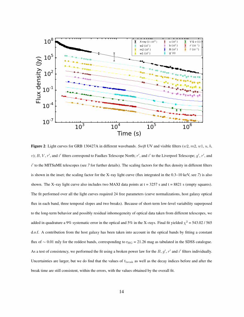
Figure 2: Light curves for GRB 130427A in different wavebands. Swift UV and visible filters (w2, m2, w1, u, b,

v); B, V , r′, and i′ filters correspond to Faulkes Telescope North; r′, and i′ to the Liverpool Telescope; g′, r′, and

i′ to the MITSuME telescopes (see 7 for further details). The scaling factors for the flux density in different filters

is shown in the inset; the scaling factor for the X–ray light curve (flux integrated in the 0.3–10 keV, see 7) is also

shown. The X–ray light curve also includes two MAXI data points at t = 3257 s and t = 8821 s (empty squares).

The fit performed over all the light curves required 24 free parameters (curve normalizations, host galaxy optical

flux in each band, three temporal slopes and two breaks). Because of short-term low-level variability superposed

to the long-term behavior and possibly residual inhomogeneity of optical data taken from different telescopes, we

added in quadrature a 9% systematic error in the optical and 5% in the X–rays. Final fit yielded χ2 = 543.02 / 565

d.o.f. A contribution from the host galaxy has been taken into account in the optical bands by fitting a constant

flux of ∼ 0.01 mJy for the reddest bands, corresponding to rHG = 21.26 mag as tabulated in the SDSS catalogue.

As a test of consistency, we performed the fit using a broken power law for the B, g′, r′ and i′ filters individually.

Uncertainties are larger, but we do find that the values of tbreak as well as the decay indices before and after the

break time are still consistent, within the errors, with the values obtained by the overall fit.

14

Figure 3. Radio (from 31: all measurements are taken at 6.8 GHz but the later one, at 7.3 GHz), optical, X–ray

(Figure 2) and LAT γ-ray (from 2) light curves of GRB 130427A and corresponding model predictions adopting

a description in terms of the van Eerten et al. model (25). To properly fit the radio data, only a fraction of the

electrons must be accelerated after ∼ 70 ks (see Table S10 and discussion in 7).

15

Figure 4. Spectral Energy Distributions (SEDs) of GRB 130427A taken at different times, from the optical to the

GeV bands (LAT data from 2). For SED 1 and SED 2 the model is a Band function, for SED 3 the model is a

Band+power law. Short dashed lines: phenomenological fit to the BAT+LAT data. Long dashed lines: results of

the van Eerten et al. model (25), with parameters discussed in (7). The different SEDs refer to the following time

intervals: 1: [0–6.5 s]; 2: [7.5–8.5 s]; 3: [8.5–196 s]; 4: [352–403 s]; 5: [406–722 s]; 6: [722–1830 s]; 7: around

3 ks; 8: around 23 ks; 9: around 59 ks; 10: around 220 ks (host galaxy contribution has been subtracted in this

case). Note that from the optical SED analysis the intrinsic extinction is negligible.

16

Supplementary Materials

www.sciencemag.org

Materials and Methods

Figures S1, S2, S3, S4, S5, S6, S7

Tables S1, S2, S3, S4, S5, S6, S7, S8, S9

References (32–62) [Note: The numbers refer to any additional references cited only within the

Supplementary Materials].

17

1 Observations and Data Analysis

1.1 Swift Discovery and Observations1.1.1 BAT Observations

BAT triggered on GRB 130427A (1) at 2013-04-27 07:47:57.5 UTC (trigger # 554620) 51.1

seconds later than the Fermi-GBM trigger (32), after Swift completed a pre-planned slew. Here-

after, all times are referred to T0,GBM so that t = T−T0,GBM. The BAT trigger was on the tail of

the main peak, in a 64-second image trigger (see (4) for details on the BAT triggering system).

The Swift slew to the source started at t = 148 s and ended at t = 192 s. The BAT position

of the burst, initially calculated onboard and then refined in ground analysis, is RAJ2000 = 11h

32m 36s.1, DecJ2000 = +27◦ 42′ 20′′.3 with an uncertainty of 1′.0 (radius, sys+stat, 90% con-

tainment); this is 49′′.9 from the radio afterglow position RAJ2000 = 11h 32m 32s.82, DecJ2000

= +27◦ 41′ 56′′.06 determined with a precision of 0′′.4 (33).

The BAT mask–weighted light curve in the 15–350 keV band is shown in Figure S1. A first

pulse beginning at t = 0.13 s and peaking at t = 0.5 s is followed by another, smaller pulse at

t = 1.1 s. Then the main episode of emission begins gradually at t = 2.2 s, with a sharp pulse

at t = 5.4 s. A multi-peaked intense emission follows, lasting a total of about 5 seconds with a

peak at t ∼ 8 s. A few, less intense pulses follow on top of a decay from the main episode, with

rise and decay on a time scale of a few seconds, the last peaking at about t = 26 s. There was

some significant deadtime over the main peak of the event, that was corrected with a maximum

correction factor of 1.72. At t = 120 s we have a fast rise with two overlapping pulses peaking

at t = 131 s and t = 141 s, respectively, followed by an exponential decay. After t = 270 s there

are no further prominent features. The decaying emission in the BAT energy range, well fit by

a power-law model, was detectable until the end of the observation at t = 2021 s. BAT data

corresponding to the last 1031 s were collected in survey mode.

18

1.1.2 XRT Observations

XRT data were accumulated in Windowed Timing (WT) and Photon Counting (PC) mode (6)

depending on the brightness of the source. The pointed Swift-XRT observations of GRB 130427A

started at t = 195 s in WT mode. Due to the loss of star tracker lock that occurred soon after

the beginning of the observation, the attitude file needed for data reduction has been manu-

ally reconstructed using the UVOT data (see section 1.1.3) to provide time-dependent pointing

corrections for the XRT data. For the subsequent observations the loss of star tracker lock oc-

curred again for several further short time intervals: data affected by bad attitude reconstruction

were adequately screened during the data reduction process. Swift-XRT observations that were

used for this work include a total net exposure time of ∼1826 s in WT mode and ∼ 203 ks in

PC mode up to the sequence 090, spread over a∼ 4 Ms baseline. The XRT data set was first pro-

cessed with the XRTDAS software package (v.2.8.0) developed at the ASI Science Data Center

(ASDC) and distributed by HEASARC within the HEASoft package (v. 6.13). Event files were

calibrated and cleaned with standard filtering criteria with the XRTPIPELINE task using the lat-

est calibration files available in the Swift CALDB. Standard grade filtering was applied: 0–12

for PC data and 0–2 for WT data. The list of all XRT observations of GRB 130427A used for

the present analysis is shown in Table S1.

The first XRT observation in WT mode partially overlaps the time interval during which

BAT data are available, from its start until t = 990 s; the remaining part is given by 1031 s of

data. The count rate of the first XRT observation was high enough to cause severe pile-up in the

WT mode data. To account for this effect, the WT data were extracted in annular regions with

a 60-pixel (1 pixel = 2.36′′) external radius and a variable radius of the inner excluded region

depending on the pile-up degree. The size of the exclusion region was determined following the

procedure illustrated in (34). The values adopted for the inner radius are reported in Table S2.

Data from light curves and spectra relevant to observations in PC mode were extracted

19

using the task XRTGRBLC, that performs the appropriate corrections for vignetting and PSF

losses. The task optimizes the extraction regions according to the count rate of the source in

each orbit, excluding a central circular region in case of pile-up (sequences 001 to 013) whose

radius is reported in Table S2. The background was extracted from an annular region with inner

and outer radii 47 and 90 pixels, respectively. Ancillary response files were generated with the

XRTMKARF task allowing us to correct for CCD defects. We used the latest CALDB response

matrices (rmf): v013 (PC mode) and v014 (WT mode).

1.1.3 UVOT Observations

Swift Ultraviolet Optical Telescope (UVOT; (5,35,36)) began observing the burst at t = 181 s.

During the automatic sequence, Swift was unable to obtain a positional lock using the onboard

catalogue as there were too few guide stars in the field of view. The loss of star tracker lock

caused the optical afterglow to wander across the image plane, so that with each consecutive

exposure the afterglow position shifted increasingly in RA and Dec away from the reported

position. For longer exposures this movement caused the point sources in the image to be

trailed. Since these observations were taken in event mode (where the position and timing of

each event are recorded down to a time resolution of 11 ms), we were able to aspect correct the

observations to a finer time resolution than the duration of each exposure and recover the trailed

sources as point sources. Because the observed and actual positions of the stars in the image

were different by up to ∼ 300′′, the aspect correction was performed in a two-step process.

First, a coarse aspect correction was determined manually for each exposure; then, a fine aspect

correction was determined by extracting an image from the event list every 10 s and cross-

correlating the stars in the image with those in the USNO-B1 catalogue. The differences in RA

and Dec were then applied to each event falling within the particular 10 s interval (37).

During the first 2 ks of observations, the optical afterglow of GRB 130427A was so bright

20

that UVOT suffered from heavy coincidence losses and scattered light. The v-band 10 s settling

point observed from t = 181 s, the majority of white data before T+2000 s, and the b and u band

data observed before 650 s could not be recovered. However, using the read-out streaks (38) we

were able to obtain photometry for the white band data between 506 and 1023 s and for the first

b and u band exposures. Earlier and later saturated white data are beyond the recommended

range for the read-out streak method. We were also able to obtain photometry from UVOT UV

grism spectrum, which provides the earliest UVOT photometry for this GRB, by folding the

spectrum through the filter response curves.

For the later follow-up observations, the star tracker obtained a positional lock on most

images, but for the observations where it failed to lock the images are trailed or the point sources

are blurred. Therefore, we manually inspected all exposures and excluded those that would

produce unreliable photometry. For the aspect corrected event mode data, the photometry was

obtained using the uvot tool UVOTEVTLC, while the image mode data were processed using the

uvot tool UVOTMAGHIST. The photometry for the image and event mode observations were

extracted using a circular aperture with a radius of 5′′ when the count rate was above 0.5 cts s−1,

and 3′′ aperture when the count rate had dropped below 0.5 cts s−1; an appropriate background

region was used. We applied coincidence loss corrections and standard photometric calibrations

(39-41). The analysis pipeline used software HEASOFT 6.13 and UVOT calibration 20130118.

The list of UVOT observations which were included in the analysis of GRB 130427A are shown

in Table S3.

Since November 2008 the automated sequence that is triggered by a strong burst includes

a 50-second UV grism exposure after the first white finder chart. A magnitude brighter than

v = 12 mag is needed to get a GRB detection. GRB 130427A provided the second good early

UV spectrum from the instrument.

The data reduction required special adaptations due to the loss of star tracker lock which

21

affected the normal processing. Using the data of detected photon positions in the white filter

prior to the grism exposure in image mode, and assuming a steady motion, the spacecraft moved

during the grism exposure by about 9.5′′(18 pixels) under an angle of 64◦ to the dispersion in

the direction of longer wavelengths. Assuming a smooth motion, this translates into a shift of

≈ 54 A in the dispersion direction.

The blurring effect of the motion on the grism image was determined by deconvolving a

zeroth order of a fainter object in the grism image by a zeroth order from an image obtained

during normal Swift operations, i.e., with attitude lock. The resulting kernel shows the exposure

locations on the detector for that zeroth order and thus suggests that the exposure was mainly

taken whilst the pointing rested in two locations about 7 pixels apart under an angle consistent

with the analysis from the white filter event data. Using that kernel to deconvolve the grism

image, a cleaner grism image was obtained where the effects of blurring are to a large extent

removed. For the deconvolution the STARLINK LUCY program was used.

To determine the position of the spectrum on the detector, the last 5 seconds of the event

data from the white filter finder were separately processed and aspect-corrected using the HEA-

SOFT 6.13 tools. This image ended 5.5 s before the start of the grism exposure, so the position

of the source on the detector in the white filter was known. Using the new grism calibration

and related software (http://www.mssl.ucl.ac.uk/www astro/uvot/) this was used to determine

the location of the spectrum on the grism image and extract the spectrum with good knowledge

of the wavelength scale.

The flux calibration used includes a correction for coincidence loss which is estimated to

be in the range of 10-20% for this spectrum. There is partial overlap of second order emission,

estimated to start affecting the flux above the observed wavelength of 3000 A by 15%, slowly

varying thereafter. The spectrum observed above 3000 A can be used to some extent for the

spectral lines present, for example, redshifted Mg II 2800 A resonance line is present as one of

22

the strongest absorptions.

The Swift UVOT spectrum with wavelengths converted to the rest frame of the GRB host is

shown in Figure S2. The wavelength scale in the UVOT grisms is not calibrated on board and its

accuracy relies on the knowledge of the position of the source. A Mg II 2800 A resonance line

seems present with a significance larger than 4 σ, although not exactly at the right frequency

location. The width of this line is larger (by a factor of two) than expected from the estimated

satellite motion from the deconvolution kernel, which would be of order of 15 A only if not

already removed by the image deconvolution.

1.2 MAXI Observations

The Gas Slit Camera (GSC; (42)) of Monitor of All-sky X–ray Image (MAXI; (15)) detected

GRB 130427A with one of its cameras (camera #4) at the two consecutive scan transits centered

at t = 3257 s and t = 8821 s. The effective area of the GSC camera during the transit had a

triangular shape with the FWZM duration of 52 seconds and the peak effective area of 3.9 cm2

at these observations. In the present analysis, we assumed the flux within a transit to be constant.

This assumption is justified considering that the time interval since the trigger (∼ thousands of

seconds) is much longer than the transit time (∼ 50 s), and therefore the variation within the

transit is negligible. MAXI usually scans a specific position in the sky once every International

Space Station orbit (≈ 92 min period). No significant flux was detected in the GSC Cameras

from the source at the last scan transit of the GRB location before the trigger (t = −2308 s) and

at the third scan after the trigger (t = +14385 s). The calibration of the energy response and

details of its flight performance is described in (43).

23

1.3 BAT and XRT Spectral Analysis

We extracted several 15–150 keV BAT spectra at different time intervals starting from t =−0.1 s

up to the end of the BAT observation. We fitted all these spectra with a simple power-law model

and the best-fit parameters are reported in Table S4. A significant spectral evolution is apparent

in the spectral results: the variation of the power-law photon index is shown in the bottom panel

of Figure S3.

In the time interval between t = 195 s and t = 990 s, corresponding to the overlap between

the BAT data and the XRT-WT data, we carried out a simultaneous broad band (0.3–150 keV)

spectral analysis, building the BAT and XRT spectra in nine common time intervals (see Ta-

ble S4). After the end of the BAT observation, the spectral analysis is based only on the 0.3–10

keV XRT data. Both the WT spectra collected between t = 990 s and t = 2021 s and the PC

spectra collected after t = 2.2 × 104 s can be well described by an absorbed power law with a

column density fixed to the line-of-sight value of 1.8× 1020cm−2 plus an intrinsic (redshifted)

and time varying (in the first 1 ks) absorption (see Table S4).

We are aware that fitting a slightly curved spectra with a power law introduces small biases

in the column density estimate (e.g. (44)). Therefore, we do not consider the column density

increase derived from power-law fitting of the afterglow data to be physically significant.

We have verified that no significant spectral variations occur during the XRT-PC monitoring,

with the power-law index consistent with a constant value. Thus we have obtained an average

PC spectrum from observation sequences 001 to 039: the results of the averaged spectral anal-

ysis are reported in Table S4.

1.4 Flux-calibrated X–ray Light Curve

We used the data from Swift-BAT, Swift-XRT and MAXI/GSC to build a flux-calibrated X–ray

light curve in the 0.3–10 keV band. We used the results of the BAT spectral analysis in the

24

15–150 keV band to compute the conversion factor needed to obtain the 0.3−10 keV flux from

the count rate of the 64 ms BAT mask-weighted light curve up to t = 202 s. This conversion

factor was computed with higher precision in the time interval in which the BAT and XRT data

overlap using the results of the simultaneous BAT and XRT spectral analysis. The 0.3–10 keV

flux for the MAXI/GSC data was obtained assuming the power-law model with a photon index

ΓM = 1.8 ± 0.1 derived from the spectral analysis carried out on XRT data at close epochs.

The 0.3−10 keV flux-calibrated light curve that we obtained is shown in Figure S3. The

good agreement between the BAT and the XRT light curves when they overlap can be inter-

preted as the sign that the early X–ray light curve (t < 103 s) is probably still related to the

prompt emission. For t > 260 s the X–ray light curve can be fitted with a double-broken

power law. The first decay is steep with α0,x = 3.32± 0.17 and a break at t1,x = 424 ± 8 s.

The decay then flattens to α1,x = 1.28 ± 0.01. A further break is needed, even if not

well constrained. The second break occurs at t2,x = 48 ± 22 ks and the slope steepens to

α2,x = 1.35 ± 0.02. We remark that it is only thanks to the very good quality of our data

that we were able to reveal this further break, whose significance is 3.8 σ, estimated through

an F-test. The reported errors are derived computing the interval for a ∆χ2 = 2.71 and are

therefore the errors at 90% confidence level for one parameter of interest. A 5% error has been

summed in quadrature to all the points to obtain a good fit with a reduced χ2red = 0.9 with 243

degrees of freedom. These decay indices and break times lie well within the distribution of

those parameters as seen for the GRB population as a whole (45,46) 1.

We plot in Figure S4 all the X–ray light curves of the GRBs observed by Swift-XRT (627

GRBs as of June 4, 2013). As it can be seen, GRB 130427A has the brightest X–ray afterglow,

in term of observed flux, that have ever been observed by XRT. But this is due both to the

intrinsic brightness of this burst and to its proximity that enhance its fluxes. A more informative

1see http://www.swift.ac.uk/xrt live cat for update versions of those populations

25

plot is the comparison of the luminosity of this GRB with those of other bright GRBs. To this

end we plot in Figure S5 the rest-frame isotropic luminosity curves for a sub-sample of GRBs

observed by Swift (both X–ray and γ-ray luminosity). We do not show the faintest GRBs,

to avoid overcrowding, and include also the brightest Fermi GRBs. As can be seen, even if

GRB 130427A has the brightest X–ray afterglow in term of observed flux, it has a normal

behavior in term of rest-frame luminosity. In fact, although it lies at the bright end, it is fully

consistent with the range displayed by the long GRBs population at large.

1.5 Ground–based Optical/NIR Observations

The 2–m Faulkes Telescope North (FTN) robotically followed up GRB 130427A starting at

t = 5.1 minutes, corresponding to ∼ 220 s in the rest frame. Observations were carried out

with a scheduled sequence of images with the B, V , r′, and i′ filters (47) for the subsequent

5 hours. From 2.4 hrs after the detection, observations were performed also with the MITSuME

Telescopes (0.5-m Akeno Observatory, 0.5-m Okayama Observatory and 1.05-m Ishigakijima

Observatory; (48)) using the g′, Rc, and Ic filters and following the optical afterglow up to

5.2 days. Data in these filters were calibrated with respect to the SDSS g′, r′, and i′ bands, re-

spectively. Late time observations have been performed also with the 2-m Liverpool Telescope

(LT) in the time interval between 1.5 days and ∼ 19 days after the burst, using the Sloan filters

SDSS-r′ and SDSS-i′.

Calibration of the entire optical data set was carried out with respect to a common set of

selected field stars. Sloan Digital Sky Survey (SDSS) catalogued stars were used for the g′,

r′ and i′ filters, while standard stars were used for the B and V filters. A summary of our

calibrated data, with a log of all the observations and magnitudes of the optical counterpart in

all filters, can be found in Tables S5–S9.

26

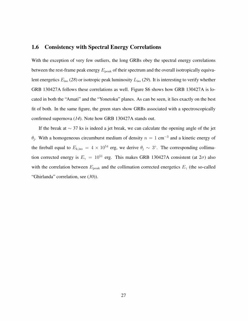
1.6 Consistency with Spectral Energy Correlations

With the exception of very few outliers, the long GRBs obey the spectral energy correlations

between the rest-frame peak energyEpeak of their spectrum and the overall isotropically equiva-

lent energeticsEiso (28) or isotropic peak luminosity Liso (29). It is interesting to verify whether

GRB 130427A follows these correlations as well. Figure S6 shows how GRB 130427A is lo-

cated in both the “Amati” and the “Yonetoku” planes. As can be seen, it lies exactly on the best

fit of both. In the same figure, the green stars show GRBs associated with a spectroscopically

confirmed supernova (14). Note how GRB 130427A stands out.

If the break at ∼ 37 ks is indeed a jet break, we can calculate the opening angle of the jet

θj. With a homogeneous circumburst medium of density n = 1 cm−3 and a kinetic energy of

the fireball equal to Ek,iso = 4 × 1054 erg, we derive θj ∼ 3◦. The corresponding collima-

tion corrected energy is Eγ = 1051 erg. This makes GRB 130427A consistent (at 2σ) also

with the correlation between Epeak and the collimation corrected energetics Eγ (the so-called

“Ghirlanda” correlation, see (30)).

27

2 Result of the SED modeling

In this section we will try to establish if the extraordinary richness and quality of data of GRB

130427A can be explained in the simple and standard framework of a relativistic fireball running

into the circumburst medium (CBM), that decelerates the fireball and produces two shocks: the

forward shock, running into the CBM, and the reverse shock, running into the ejected material of

the fireball. To this aim we adopt a publicly available model, developed by (25), that captures

with some details the main physical processes we believe are occurring. On the other hand,

reality is surely more complex than a simple standard model can account for. There can be

more specific versions of the standard model, e.g. the fireball could be structured (namely,

having an angular profile of bulk Lorentz factors and energies), the CBM could be clumped,

the microphysical parameters could be varying in time and in space. However, all these are

“versions” of the standard model (a collimated fireball running into the CBM) that we aim to

test in its pillars, and not in its “details”. We therefore ask: does the basic model reasonably

account for the observed properties of this data–rich burst, or should we drastically reconsider

our current general view of GRB physics?

2.1 Main assumptions

The similarity of the X–ray and optical light curves after ∼ 104 seconds suggests that they are

produced by the same process. The similarity of their spectral indices indicates that they belong

to the same power-law spectrum. Therefore, we assume that the optical and the X–ray emission,

after∼ 104 seconds, are both afterglow emission produced by a forward shock. Before 104 s, an

extra component contributes to the emission, most notably in the X–rays. This extra component

could be late prompt emission or reverse shock emission, but we will not model it.

The Fermi–LAT emission, above 100 MeV, is not correlated with the ∼ MeV emission as

shown by the GBM or BAT, but shows a peak at ∼ 20 seconds followed by a power-law decay

28

(see (2)). These properties suggest that the Fermi-LAT flux is afterglow emission produced

by a forward shock. The peak of the emission indicates the onset of the afterglow. We also

assume that the LAT luminosity above 100 MeV is a proxy of the bolometric luminosity of the

afterglow. This should be truly independent of the radiation process originating this high-energy

emission.

We assume that the radio emission could either be the low frequency part of the X–ray and

optical forward shock emission, or instead be due to a reverse shock as suggested by (31). In

the latter case our afterglow model, with no reverse shock emission, should underestimate the

observed radio emission.

We assume that the achromatic break in the light curves at ∼ 37 ks is a jet break.

2.2 General derived properties

Density profile — In the case of a homogeneous density, Lbol increases during the coasting

phase (Γ=constant) as the observed surface area, hence as t2. If the circumburst medium has a

wind density profile n ∝ R−2, the increase of the observed surface area in the coasting phase is

exactly compensated by the decreasing density, and the bolometric luminosity is constant (see,

e.g., (49) and Eq. 11 in (50)). After the deceleration time, for an adiabatic fireball we have

Lbol ∝ t−1 both for the homogeneous and the wind density profile, as long as the emission

occurs in the fast cooling regime. This is independent from the radiation process producing the

LAT flux [e.g. synchrotron or synchrotron self–Compton (SSC)].

There exists the possibility that the GeV peak is produced by a reverse shock, possibly

connected with the early optical flux (10). However, in this case, the decay slope of the optical

flux depends on the density profile, and if it is wind–like, it is steeper than observed (51).

The flux decay after the peak is suggestive of an homogeneous medium if the GeV emission

is SSC, since a wind density profile would make the GeV light curve substantially steeper than

29

observed (this point is made very explicitly by (26)). If the GeV is synchrotron, instead, we

face the problem of explaining the nature of the very energetic photons (up to 130 GeV, rest

frame) that are not expected in a shock acceleration scenario (see discussion in (2)). Another

problem, shown in Fig. 11 of (52), is the over–prediction of the flux at early times (t < 300 s)

in the Swift-BAT and Fermi-LAT energy ranges.

A wind medium has been assumed to reproduce the X–ray/optical/radio data of GRB 130427A

(31,52) and to explain the early optical flux (10). In (31), the wind like density is preferred by

comparing the predicted and observed X–ray decay slope. The slope predicted by the homoge-

neous density is closer to the observed decay. Nevertheless, they chose the wind density profile

(compare the following values derived by (31): predicted decay in the wind case: αx = 1.64,

in the homogeneous case: αx = 1.14, observed value: αx = 1.35). Furthermore, their wind

afterglow model requires a kinetic energy Ek,iso ∼ 1052 erg, which is only 1% of the prompt

emission energy (Eγ,iso = 1054 erg), which seems rather low. This small value of Ek,iso implies

rather large values of the microphysical parameters: εB and εe are of order unity. As a conse-

quence, the εe/εB ratio is also of order unity, and this limits the possibility to explain the GeV

emission as due to the SSC process. It is then difficult to explain the detection of photons up

to 130 GeV (rest frame). The normalization of the wind density profile is roughly 1,000 times

smaller than expected by a typical star wind, even if this parameter is still largely uncertain for

the (unknown) final phases of the life of a massive star.

Finally, we have considered a generic stratified medium, with a density n ∝ r−s, with s = 1

and s = 1.5, following (53), with the hope to ameliorate the problems of the pure wind–like

scenario. We did find that these solutions present a deceleration peak flux, that can explain the

peaked GeV emission, but are worst representations of the data at the other frequencies.

To conclude, i) the presence of the peak of the light curve and ii) the relatively flat decay

slope of the light curves at all frequencies are observational evidences supporting the homoge-

30

neous CBM. Further support of this hypothesis is given by the small kinetic energy (requiring

very large efficiencies) and the small wind normalization required by the proposed wind mod-

els. The latter are certainly possible, but the required (not mainstream) assumptions and the

remaining open issues, in our opinion, are more than in the homogeneous case, that therefore

we choose.

Bulk Lorentz factor — The time of the onset of the afterglow, for an assumed radiative

efficiency η (defined through Eiso = ηEk,iso, where Ek,iso is the isotropic equivalent kinetic

energy of the fireball) and ISM density n, allows us to infer the value of the bulk Lorentz factor

Γ0 of the fireball before deceleration, i.e. during the coasting phase (see the discussion in (24)

about the existing formulae). For Eγ,iso = 1054 erg s−1, η = 0.1, tpk = 20 s and a density n = 1

cm−3 we obtain Γ0 = 505 (using the formula in (24)), scaling as Γ0 ∝ [Eγ,iso/(nηt3pk)]

1/8.

Microphysical parameters: εB — The fraction of the available energy at the relativistic shock

going to relativistic electrons and to magnetic energy is parameterized by εe and εB, respectively.

The fact that the X–ray and the optical light curves share the same temporal profile in the

104–106 s interval implies that they belong to the same spectral power law branch. Therefore

the characteristic frequencies, such as the injection frequency νinj or the cooling frequencies

νcool, that are time–dependent, must be located outside the optical–X–ray frequency range in

this time interval because, otherwise, the light curves could not be parallel. The requirement

νcool ∼> 10 keV can be fulfilled if εB is small (of the order of 10−5–10−4) implying a modest

cooling (in turn implying a large νcool). This small value of εB is not unprecedented, since it

agrees with those found by (54) for the GRBs detected in the GeV band by the LAT on board

Fermi. However, more often εB is around ∼ 10−2 − 10−3 (19,53).

Microphysical parameters: εe — If the LAT emission is afterglow by a forward shock, and

if it is a good proxy for the bolometric luminosity (LLAT = f Lbol), we can derive εe. In the

31

fast cooling regime, LLAT after the deceleration time is given by (see e.g. (24))

LLAT = f Lbol =3fεe

2

Ekin,iso

t; t ≥ tpk; Ekin,iso = Eγ,iso

(1− ηη

)(1)

therefore

εe ∼2

3f

η

1− ηLLAT

Eγ,isotpk (2)

With Eγ,iso ∼ 1054 erg, η = 0.1, f ∼ 1/6 and LLAT ∼ 1.6 × 1051 erg s−1 at tpk ∼ 15 s (in the

rest frame), we derive εe ∼ 10−2. Notice that this is independent of the emission process (see

the discussion after Eq. 1 in (55)).

Jet opening angle and viewing angle — Defining the viewing angle θv as the angle between

the line of sight and the jet axis, we have that a non–zero θv produces two breaks in the light

curve, the first when 1/Γ = θj − θv, and the second when 1/Γ = θj + θv. With respect to

an observer located on the jet axis (θv = 0) the off–axis viewer should see the jet break as

a smoother transition (e.g. (25,56)). This could help make the post–break light curve decay

less steeply than predicted, as in our case, up to the second break. The latter could be hidden

in the optical by the host galaxy+supernova contribution to the light curve flux, but should be

visible in the X–ray light curve. Note that a shallow break can also be the result of time-varying

microphysical parameters: if εB and εe increase, then the light curve decays less steeply than

predicted by the simplest theory, at least up to the time when εB and εe stop increasing (since

the range of their values is limited). After that time, the light curve should decay as expected

by the simple theory.

Radio spectra — The available radio data (as in (31)) indicate a rather flat spectrum, in-

consistent with self–absorption and roughly consistent with Fν ∝ ν1/3, the single electron

synchrotron spectrum. This indicates that in the radio range νa < ν < νinj. A small νa in turn

requires a small density (of the relativistic electrons responsible for the synchrotron emission

32

and absorption), much smaller than the typical value of n ∼ 1 cm−3. A large νinj ∝ γ2injBΓ

requires large energies of the electrons.

2.3 Modeling

The model — To model the SEDs and the light curves at any frequency of GRB 130427A we

use the model developed by (25). This model considers the synchrotron emission produced by

the forward shock of an adiabatic fireball expanding into a homogeneous medium. The fireball

is canonical (namely, matter, not magnetically dominated, and uniform, i.e. with radial velocity

directions that are not a function of the angle from the jet axis) with an opening angle θj, viewed

at an angle θv from the axis. It accounts for the so called “jet–break”, i.e the break in the light

curve occurring when 1/Γ ∼ θj. Arrival times from the emitting volume are properly calculated.

The model does not include the emission from the reverse shock, nor the contribution from

synchrotron self–Compton (SSC) process. The lack of SSC is a rather serious limitation in

the first (fast cooling) phases of the afterglow if the Comptonization parameter y (regulating

the importance of the SSC radiation) is large, while in slow cooling the importance of SSC

radiation rapidly decreases. Although we require a small εB, and y ∼ (εe/εB)1/2 (see above),

our modeling pertains to the slow cooling phase, therefore the lack of SSC does not affect our

results. Table S10 lists the parameters of the models shown in Figure S7 (light curves) and

Figure 3 of the main journal article (SEDs).

The LAT light curve — As mentioned above, the time profile of the bolometric light curve

in fast cooling is independent of the emission process. If the LAT flux is indeed close to the

bolometric flux, then its behavior cannot be used to discriminate between – say – synchrotron

and SSC emission, provided that both processes are capable of generating high-energy photons.

For GRB 130427A photons exceeding 40 GeV have been observed, with one exceeding 90 GeV,

and this represents a problem for the synchrotron interpretation of the high-energy flux (see, e.g.

33

(57)). On the other hand, both SSC and inverse Compton scattering between the accelerated

electrons and the prompt emission photons still present in the fireball can contribute to the GeV

flux. This is even more likely if εB is indeed very small. In this case the Comptonization y

parameter is bound to be large in fast cooling, making the Compton process the dominant one

(unless the synchrotron typical frequencies, in the comoving frame, are so large as to make the

Compton process to be in the Klein–Nishina regime).

Ghisellini et al. (55) discussed the case of a radiative fireball to explain the time decay of

several GRBs whose γ–ray flux decayed as t−1.5 even though their spectral slope was close to

Γγ = 2. The decay slope of GRB 130427A is instead close to unity, i.e. what is expected from

the bolometric luminosity decay of an adiabatic fireball. This can be explained if we consider

that in GRB 130427A the afterglow onset time is close to 15 seconds: this may appear to be

a very short time, but it is nevertheless later than the onset time of the bursts considered in

(55). This relatively late onset implies that the total energy emitted in the LAT energy band is

significantly lower than the prompt emission energy. If the prompt emission did not contain

a sizable fraction of the kinetic energy of the fireball, then Ek ∼ Eγ,iso/η and does not vary

during the γ–ray emission. In other words, the fireball remains adiabatic or quasi–adiabatic.

We stress that if the ISM had a wind density profile, then the initial light curve of the bolometric

luminosity would be flat, without any peak. Therefore an homogeneous medium is consistent

with interpreting the peak of the LAT light curve as the afterglow onset, while a wind density

profile would require another interpretation for the same peak.

The XRT light curve — The model reproduces the X–ray light curve after ∼ 104 seconds.

We suggest that before this time the X–ray flux is dominated by late prompt emission and

high–latitude radiation. By “late prompt” emission we mean radiation produced by the same

mechanism(s) producing the main GRB event, but occurring later. By “high–latitude” radiation

we mean the radiation from parts of the emitting surface not on axis with the line of sight. If

34

the surface switches off abruptly, the distant observer will see that a flux decaying in time at

a predictable rate, as a result of the different arrival time of the photons combined with the

different degree of beaming. Indeed, the XRT and BAT light curves are very similar as long as

BAT detects the burst (∼1900 seconds).

The optical–UV light curve — In Figure S7 we show how the model reproduces the best

sampled optical light curves, in the R, r′ and Rc filters. In the other optical bands the behavior

is the same. In the model of the optical emission shown in Figure S7, we have added a constant

contribution corresponding to R = 21.3 (flux density ∼0.0113 mJy) due to the host galaxy

(dashed line in Figure S7).

Jet break — We interpret the break at ∼ 37 ks as a jet break, corresponding to a jet open-

ing angle of ∼ 3.4◦. We assume θv = 0◦. In fact, although the assumption of a non–zero

θv could help to explain the shallow decay of the post–break light curve (∝ t−1.3, shallower

than predicted by the standard model, e.g. (58)), the late X–ray data (not affected by the host

galaxy+supernova emission) do not show any further steepening of the light curve up to t ∼ 45

days. We are then led to assume that the radiation emitted in the post–break phase is larger

than what simple theory predicts (shown by the dotted models in Figure S7). This can be the

result of having energy injection, increasing the total fireball energy which in turn increases

the amount of emitted radiation. Alternatively, we can maintain a constant fireball energy, but

increase the amount of energy given to the electrons (i.e. εe). We prefer the latter solution be-

cause it has a lower energy requirement. We then assume that εe ∝ (t/tε)0.6 after tε = 0.8 day.

Then, to obtain a reasonable agreement between the optical and X–ray data (circles and crosses

in Figure S7) and the model, we also assume that εB ∝ (t/tε)0.5 after the same tε = 0.8 day.

Possible evolution of the microphysical parameters at the shocks have been invoked to explain

the multiwavelength light curves (in the X–ray and optical bands) of some GRBs (e.g. (59)).

35

The radio light curve — The model that we have described above, which assumes an evo-

lution of the εe and εB parameters, over–predicts the radio flux (dot–dashed line vs squares in

Figure S7). This is due to the fact that the νinj frequency is too small and it is even smaller

than the self–absorption frequency νa. The injection frequency is νinj ∝ γ2injBΓ ∝ ε2eε1/2B t−3/2.

Changing the microphysical parameters inevitably leads to other inconsistencies. An extra de-

gree of freedom is the fraction of the electrons that are accelerated at the shock front and that

produce the radiation received by the observer. Instead of assuming that the shock accelerates

one electron per proton, we can assume that only a fraction k < 1 of the present electrons are

accelerated. In this way we can increase the energy per electron and, therefore, increase νinj.

This, however, must occur in such a way as to satisfy the requirement that νinj is smaller than the

observed optical frequencies, at least between 104 and 106 seconds, if the optical flux remains a

power law of the same slope in this time interval.

Admittedly, the complex behavior of the afterglow of GRB 130427A in the radio, optical,

X–ray and γ–ray bands cannot be fully captured by a simple and standard afterglow model, e.g.

synchrotron and self Compton emission by a forward shock, with non-varying microphysical

parameters. Therefore we must ask ourselves: does GRB 130427A require a complete revision

of our ideas about the origin of the afterglow emission? Our answer is no: the unique richness

of the GRB 130427A data can still be explained within the framework of the standard model. It

surely requires extra assumptions, but not a radical change.

36

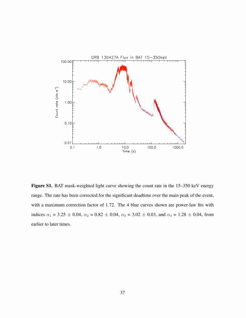
Figure S1. BAT mask-weighted light curve showing the count rate in the 15–350 keV energy

range. The rate has been corrected for the significant deadtime over the main peak of the event,

with a maximum correction factor of 1.72. The 4 blue curves shown are power-law fits with

indices α1 = 3.25 ± 0.04, α2 = 0.82 ± 0.04, α3 = 3.02 ± 0.03, and α4 = 1.28 ± 0.04, from

earlier to later times.

37

1400 1600 1800 2000 2200 2400 2600 2800 3000

at z=0.34 restframe λ(◦A)

0.5

1.0

1.5

2.0

2.5

3.0

3.5

flux (erg/cm

2/s/◦ A)

1e 13

Mg IIMg II

GRB130427A Swift UVOT uv grism

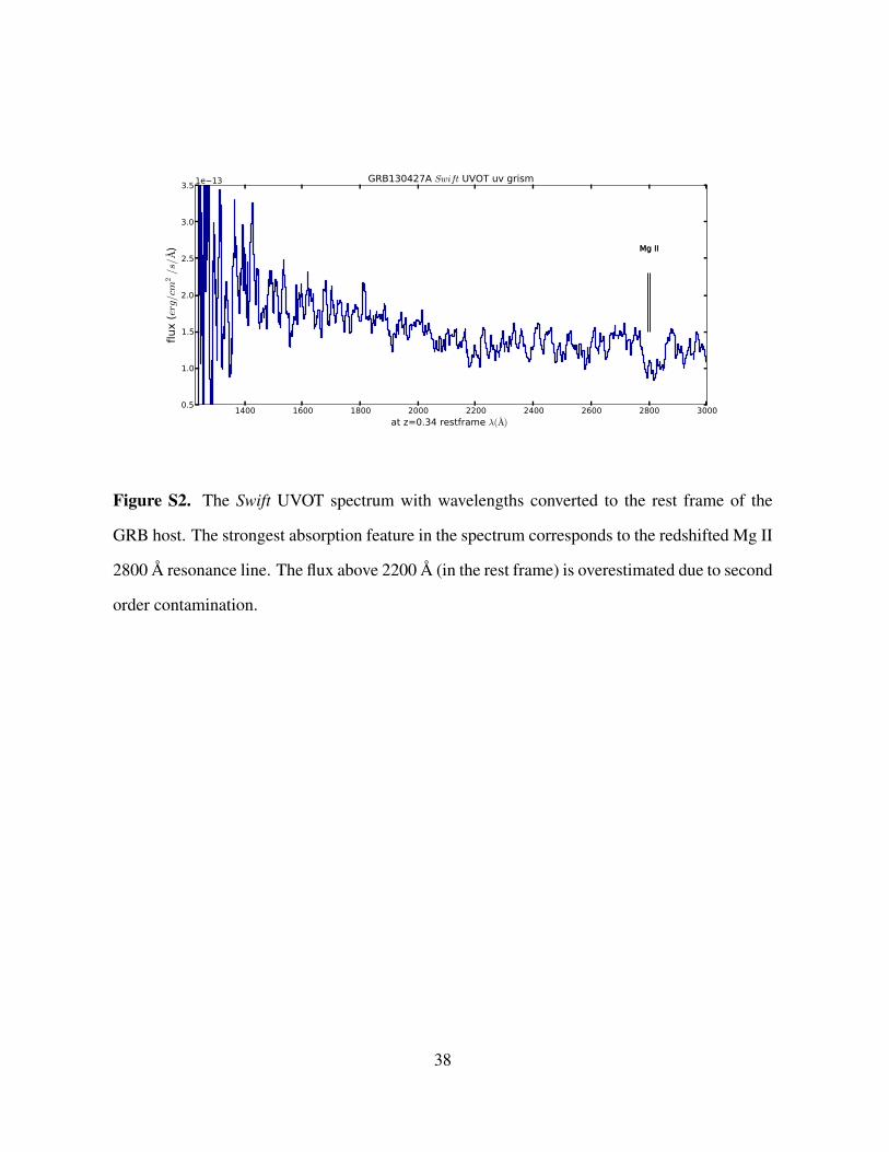
Figure S2. The Swift UVOT spectrum with wavelengths converted to the rest frame of the

GRB host. The strongest absorption feature in the spectrum corresponds to the redshifted Mg II

2800 A resonance line. The flux above 2200 A (in the rest frame) is overestimated due to second

order contamination.

38

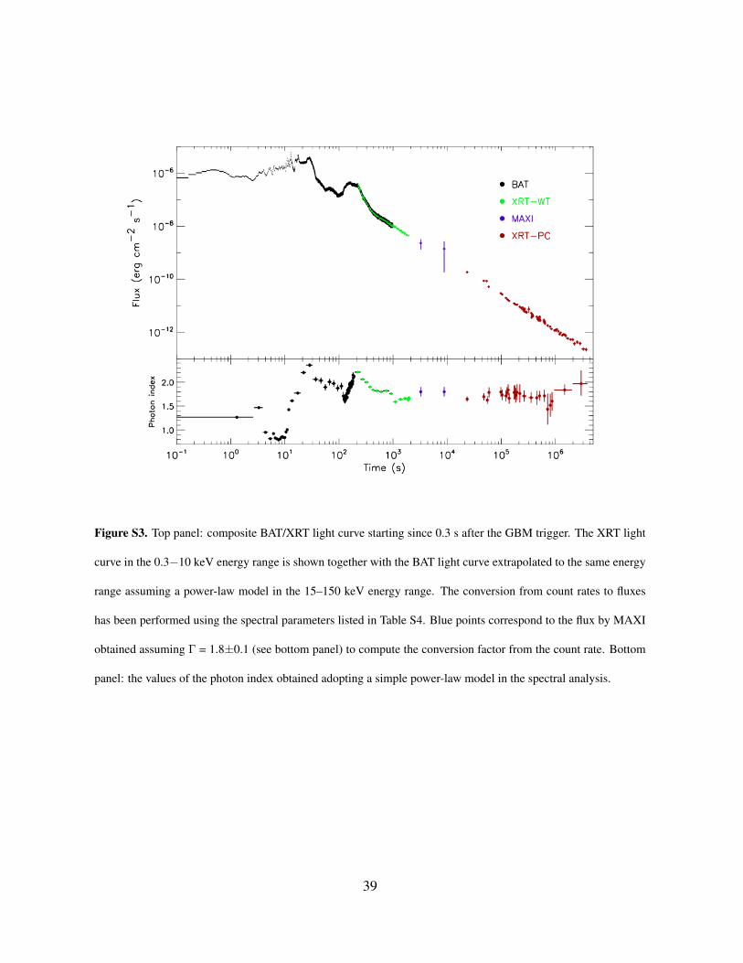
Figure S3. Top panel: composite BAT/XRT light curve starting since 0.3 s after the GBM trigger. The XRT light

curve in the 0.3−10 keV energy range is shown together with the BAT light curve extrapolated to the same energy

range assuming a power-law model in the 15–150 keV energy range. The conversion from count rates to fluxes

has been performed using the spectral parameters listed in Table S4. Blue points correspond to the flux by MAXI

obtained assuming Γ = 1.8±0.1 (see bottom panel) to compute the conversion factor from the count rate. Bottom

panel: the values of the photon index obtained adopting a simple power-law model in the spectral analysis.

39

Figure S4. Comparison of all the 627 GRBs observed by XRT (as of June 4, 2013). In terms of the observed flux,

the X–ray afterglow of GRB 130427A, in red color in this figure, is the brightest so far observed.

40

10-10

10-8

10-6

10-4

10-2

1

102

10-2 10-1 1 101 102 103 104 105 106 107

L X

(*10

51 e

rg s

-1)

Time (s)

080319B130427A

Figure S5. Rest–frame isotropic X–ray luminosity light curves for a selected sample of long, relatively bright

GRBs (grey curves). For comparison we show in orange and blue the rest–frame luminosity for GRB 130427A

and GRB 080319B (naked-eye), respectively. For each event we also plot the BAT γ-ray luminosity. The behavior

and luminosity of GRB 130427A is within the range of long GRBs population at large.

41

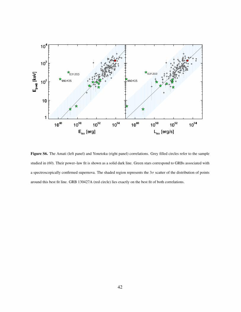
Figure S6. The Amati (left panel) and Yonetoku (right panel) correlations. Grey filled circles refer to the sample

studied in (60). Their power–law fit is shown as a solid dark line. Green stars correspond to GRBs associated with

a spectroscopically confirmed supernova. The shaded region represents the 3σ scatter of the distribution of points

around this best fit line. GRB 130427A (red circle) lies exactly on the best fit of both correlations.

42

Line Ek εe εB n p θj tk αk te αe tB αB

erg/s cm−3 deg days days daysdotted 5e54 0.027 1.e–5 1 2.3 3.4◦ ... ... ... ... ... ...solid 5e54 0.027 1.e–5 1 2.3 3.4◦ 0.2 –0.8 0.8 0.6 0.8 0.5

Table S10. List of parameters used for the model plotted in the Figure S7. We assumed k = (t/tk)αk after tk(and same functions for εe and εB).

Figure S7. The optical, X–ray, γ–ray and radio light curves are interpreted as forward shock afterglow synchrotron

emission, as derived applying the van Eerten et al. model. Dotted lines corresponds to the first line in Table S10,

namely εe, εB and the fraction k of accelerated electrons are constant. The solid line corresponds to the model

when varying these microphysical parameters. The dot–dashed line shown only for the radio band, corresponds to

the model with only εe and εB varying in time and with constant k.

43

Date ObsID Mode tstart tstop Exposure2013-04-27 00554620000 WT 195.0 2021.0 1826.02013-04-27 00554620001 PC 22895.7 23992.1 1091.32013-04-27 00554620002 PC 46969.2 48157.6 1183.72013-04-27 00554620003 PC 53000.0 57444.6 1166.22013-04-28 00554620010 PC 58984.1 59841.1 616.82013-04-28 00554620011 PC 86273.6 86308.9 34.92013-04-28 00554620012 PC 97700.2 98876.9 1171.22013-04-28 00554620013 PC 103473.2 104649.1 1171.22013-04-28 00554620014 PC 121583.6 122777.0 1188.72013-04-28 00554620015 PC 127497.0 128688.0 1186.22013-04-28 00554620016 PC 133486.8 134678.1 1186.22013-04-28 00554620017 PC 139453.2 140626.6 1168.72013-04-29 00554620018 PC 172691.4 173887.4 1191.22013-04-29 00554620019 PC 178457.6 179653.6 1191.22013-04-29 00554620020 PC 184342.2 185538.2 1191.22013-04-29 00554620021 PC 195806.2 197002.1 1191.22013-04-29 00554620022 PC 214255.0 214282.9 27.42013-04-29 00554620023 PC 220516.4 226200.7 1163.72013-04-30 00554620024 PC 236492.8 284417.9 2235.02013-04-30 00554620025 PC 231962.4 295404.9 1263.62013-05-01 00554620026 PC 318431.4 387978.9 2949.32013-05-01 00554620027 PC 323916.2 393026.9 2861.82013-05-02 00554620028 PC 443986.8 480197.1 2474.82013-05-02 00554620029 PC 450022.2 462502.1 1033.82013-05-03 00554620030 PC 495862.2 520641.9 4879.12013-05-03 00554620031 PC 501622.2 525617.9 4033.12013-05-04 00554620032 PC 611311.6 636145.9 4869.62013-05-04 00554620033 PC 617072.2 642158.1 3628.52013-05-05 00554620034 PC 711244.4 734065.1 948.92013-05-05 00554620035 PC 717012.8 728662.1 946.4

Table S1. List of XRT Observations.

44

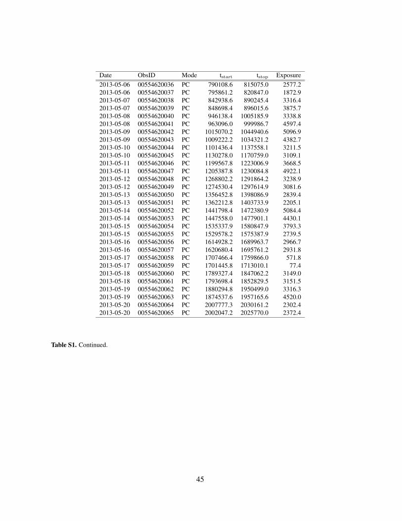
Date ObsID Mode tstart tstop Exposure2013-05-06 00554620036 PC 790108.6 815075.0 2577.22013-05-06 00554620037 PC 795861.2 820847.0 1872.92013-05-07 00554620038 PC 842938.6 890245.4 3316.42013-05-07 00554620039 PC 848698.4 896015.6 3875.72013-05-08 00554620040 PC 946138.4 1005185.9 3338.82013-05-08 00554620041 PC 963096.0 999986.7 4597.42013-05-09 00554620042 PC 1015070.2 1044940.6 5096.92013-05-09 00554620043 PC 1009222.2 1034321.2 4382.72013-05-10 00554620044 PC 1101436.4 1137558.1 3211.52013-05-10 00554620045 PC 1130278.0 1170759.0 3109.12013-05-11 00554620046 PC 1199567.8 1223006.9 3668.52013-05-11 00554620047 PC 1205387.8 1230084.8 4922.12013-05-12 00554620048 PC 1268802.2 1291864.2 3238.92013-05-12 00554620049 PC 1274530.4 1297614.9 3081.62013-05-13 00554620050 PC 1356452.8 1398086.9 2839.42013-05-13 00554620051 PC 1362212.8 1403733.9 2205.12013-05-14 00554620052 PC 1441798.4 1472380.9 5084.42013-05-14 00554620053 PC 1447558.0 1477901.1 4430.12013-05-15 00554620054 PC 1535337.9 1580847.9 3793.32013-05-15 00554620055 PC 1529578.2 1575387.9 2739.52013-05-16 00554620056 PC 1614928.2 1689963.7 2966.72013-05-16 00554620057 PC 1620680.4 1695761.2 2931.82013-05-17 00554620058 PC 1707466.4 1759866.0 571.82013-05-17 00554620059 PC 1701445.8 1713010.1 77.42013-05-18 00554620060 PC 1789327.4 1847062.2 3149.02013-05-18 00554620061 PC 1793698.4 1852829.5 3151.52013-05-19 00554620062 PC 1880294.8 1950499.0 3316.32013-05-19 00554620063 PC 1874537.6 1957165.6 4520.02013-05-20 00554620064 PC 2007777.3 2030161.2 2302.42013-05-20 00554620065 PC 2002047.2 2025770.0 2372.4

Table S1. Continued.

45

Date ObsID Mode tstart tstop Exposure2013-05-21 00554620066 PC 2093589.6 2128184.9 4123.02013-05-21 00554620067 PC 2099349.3 2122434.4 1470.92013-05-22 00554620068 PC 2180242.6 2215409.1 1815.52013-05-22 00554620069 PC 2185857.8 2210360.0 4065.62013-05-24 00554620070 PC 2358988.2 2382118.1 1643.22013-05-24 00554620071 PC 2364683.4 2389163.0 4567.52013-05-26 00554620072 PC 2520513.0 2543605.9 112.42013-05-26 00554620073 PC 2514753.2 2537833.9 127.42013-05-28 00554620074 PC 2687649.2 2712052.5 2584.72013-05-28 00554620075 PC 2693409.2 2723792.9 3341.42013-05-30 00554620076 PC 2838150.4 2873300.8 2517.32013-05-30 00554620077 PC 2843910.2 2878100.5 182.32013-05-31 00554620078 PC 2958738.2 2970872.2 1530.92013-06-01 00554620079 PC 3034154.0 3058480.6 4260.42013-06-01 00554620080 PC 3039807.5 3064297.5 3498.72013-06-03 00554620081 PC 3207534.7 3219986.9 964.02013-06-03 00554620082 PC 3196010.0 3224848.9 112.42013-06-05 00554620083 PC 3385650.6 3426578.8 2632.12013-06-05 00554620084 PC 3380735.1 3420857.9 3184.02013-06-07 00554620085 PC 3524157.8 3548402.3 3611.12013-06-07 00554620086 PC 3518412.8 3542624.9 3443.82013-06-09 00554620087 PC 3691594.0 3726982.5 1970.42013-06-09 00554620088 PC 3697361.2 3698268.8 904.02013-06-11 00554620089 PC 3870322.0 3906218.0 2627.12013-06-11 00554620090 PC 3864659.2 3899309.9 1223.7

Table S1. Continued.

46

Mode tstart tstop r RWT 195 250 30 60WT 250 300 20 60WT 300 350 15 60WT 350 400 12 60WT 400 450 10 60WT 450 550 9 60WT 550 650 8 60WT 650 850 7 60WT 850 1150 4 60WT 1150 1851 3 60

PC 22874 54172 4 32PC 57429 59534 2 27

Table S2. The value, expressed in pixels (1 pixel = 2.36′′), of the inner r and outer R radius of the annular extraction

region adopted to take into account the pile-up corrections, when needed.

47

tstart Time interval Flux Magnitude Filters s mJy mag

432.9 19.4 55.86 ± 1.78 12.10 ± 0.04 v606.5 19.7 38.62 ± 1.18 12.50 ± 0.03 v779.2 19.7 31.23 ± 0.98 12.73 ± 0.04 v

1104.7 19.7 19.01 ± 0.67 13.27 ± 0.04 v1278.7 19.7 16.55 ± 0.60 13.42 ± 0.04 v1450.9 19.7 13.92 ± 0.54 13.61 ± 0.04 v1623.2 19.2 11.90 ± 0.50 13.78 ± 0.05 v1795.5 176.8 10.87 ± 0.42 13.88 ± 0.04 v1972.3 15.8 10.77 ± 0.51 13.89 ± 0.05 v

221178.8 79.8 0.042 ± 0.025 19.91 ± 0.54 v271227.3 24196.7 0.019 ± 0.016 20.72 ± 0.69 v358892.1 23111.9 0.050 ± 0.009 19.70 ± 0.19 v462312.3 46771.8 0.020 ± 0.006 20.68 ± 0.32 v520269.5 394.6 0.017 ± 0.010 20.84 ± 0.53 v612573.7 23590.4 0.021 ± 0.006 20.66 ± 0.30 v797123.6 64580.4 0.016 ± 0.006 20.94 ± 0.37 v884582.0 79902.1 0.006 ± 0.009 22.03 ± 1.07 v981779.5 63164.5 0.012 ± 0.004 21.23 ± 0.37 v

1102735.3 110088.8 0.015 ± 0.005 21.00 ± 0.35 v1270046.2 128057.8 0.015 ± 0.005 20.97 ± 0.35 v1443096.2 29287.8 0.018 ± 0.006 20.81 ± 0.33 v1615695.2 208.9 0.035 ± 0.015 20.11 ± 0.42 v1800561.6 149962.6 0.014 ± 0.005 21.08 ± 0.39 v2008769.3 206654.8 0.013 ± 0.004 21.15 ± 0.34 v

Table S3. UVOT Observation log, reporting the interval of time over which observations have been collected since

tstart. Observations where reliable photometry could not be extracted are not included in the table. Magnitudes

have not been corrected for Galactic absorption along the line of sight (EB−V = 0.020 mag; (61)). The estimate

extinctions in the different filters are: Av = 0.062 mag, Ab = 0.079 mag, Au = 0.096 mag, Aw1 = 0.132 mag, Am2

= 0.193 mag, and Aw2 = 0.175 mag. Corrected magnitudes have been converted into flux densities, Fν , following

(62).

48

tstart Time interval Flux Magnitude Filters s mJy mag

531.3 19.8 111.71 ± 41.54 11.48 ± 0.56 b705.2 19.7 30.25 ± 1.04 12.90 ± 0.04 b877.1 19.7 23.12 ± 0.71 13.19 ± 0.04 b

1202.9 19.7 16.05 ± 0.48 13.59 ± 0.03 b1376.9 19.7 13.11 ± 0.39 13.81 ± 0.03 b1549.3 19.7 11.28 ± 0.34 13.97 ± 0.04 b1721.3 19.6 10.22 ± 0.32 14.08 ± 0.04 b1894.7 19.7 9.96 ± 0.31 14.10 ± 0.04 b

214507.9 6340.9 0.076 ± 0.013 19.40 ± 0.18 b271079.9 24046.0 0.048 ± 0.009 19.88 ± 0.21 b358368.0 23153.4 0.026 ± 0.004 20.55 ± 0.16 b461774.3 46475.9 0.020 ± 0.003 20.81 ± 0.16 b519400.6 428.8 0.026 ± 0.005 20.55 ± 0.21 b611734.9 23645.7 0.016 ± 0.003 21.05 ± 0.19 b728222.7 68475.9 0.017 ± 0.003 21.03 ± 0.22 b849077.3 35320.8 0.012 ± 0.003 21.40 ± 0.28 b963459.9 80954.7 0.011 ± 0.002 21.47 ± 0.20 b

1101871.9 110119.4 0.012 ± 0.002 21.37 ± 0.21 b1269219.5 128289.1 0.008 ± 0.002 21.79 ± 0.29 b1442233.5 93695.0 0.013 ± 0.002 21.33 ± 0.21 b1615186.9 144686.9 0.009 ± 0.005 21.62 ± 0.49 b1799842.9 150091.8 0.009 ± 0.003 21.70 ± 0.30 b2008110.9 206950.9 0.012 ± 0.003 21.37 ± 0.24 b

Table S3. Continued.

49

tstart Time interval Flux Magnitude Filters s mJy mag

506.3 19.8 52.75 ± 18.58 11.19 ± 0.35 u680.3 5.9 25.06 ± 1.61 12.00 ± 0.07 u852.4 19.7 21.97 ± 0.73 12.14 ± 0.04 u

1178.1 19.7 14.55 ± 0.44 12.59 ± 0.04 u1352.2 19.7 11.68 ± 0.34 12.83 ± 0.03 u1524.0 19.7 10.67 ± 0.31 12.93 ± 0.03 u1696.3 19.7 9.42 ± 0.29 13.06 ± 0.04 u1870.0 19.7 8.52 ± 0.26 13.17 ± 0.04 u

54067.8 93.6 0.335 ± 0.017 16.69 ± 0.06 u59780.3 83.7 0.281 ± 0.018 16.88 ± 0.07 u

140625.7 25.7 0.113 ± 0.021 17.86 ± 0.20 u214423.1 11801.4 0.049 ± 0.005 18.76 ± 0.13 u294833.7 143.7 0.044 ± 0.007 18.89 ± 0.17 u358106.2 23165.6 0.028 ± 0.002 19.38 ± 0.10 u461504.8 41819.3 0.016 ± 0.002 20.01 ± 0.14 u514722.8 10921.3 0.025 ± 0.005 19.48 ± 0.20 u611315.7 30848.3 0.013 ± 0.001 20.22 ± 0.12 u717016.8 11200.7 0.016 ± 0.002 20.01 ± 0.17 u795865.5 83118.5 0.011 ± 0.001 20.40 ± 0.13 u884045.8 79408.9 0.007 ± 0.001 20.81 ± 0.23 u980566.2 63564.7 0.008 ± 0.001 20.69 ± 0.15 u

1101440.8 110128.2 0.009 ± 0.001 20.59 ± 0.18 u1218440.7 69083.4 0.003 ± 0.001 21.91 ± 0.45 u1356456.8 121447.2 0.005 ± 0.001 21.25 ± 0.22 u1530645.2 142918.7 0.006 ± 0.001 21.02 ± 0.25 u1759348.6 173006.9 0.005 ± 0.001 21.18 ± 0.24 u1945016.0 178788.1 0.003 ± 0.001 21.67 ± 0.33 u2187205.5 27676.8 0.002 ± 0.002 22.38 ± 0.93 u

Table S3. Continued.

50

tstart Time interval Flux Magnitude Filters s mJy mag

556.8 20.0 52.22 ± 13.70 11.52 ± 0.27 white729.7 20.0 28.38 ± 11.16 12.18 ± 0.39 white924.4 150.0 18.79 ± 4.55 12.63 ± 0.26 white

271152.9 24121.4 0.041 ± 0.003 19.28 ± 0.09 white358629.3 23141.3 0.028 ± 0.002 19.67 ± 0.06 white462042.5 46641.4 0.019 ± 0.001 20.10 ± 0.07 white519834.3 428.8 0.018 ± 0.002 20.13 ± 0.12 white612153.5 23645.9 0.014 ± 0.001 20.43 ± 0.09 white728641.2 68476.1 0.013 ± 0.002 20.52 ± 0.16 white849450.8 35125.5 0.011 ± 0.002 20.68 ± 0.13 white963818.3 80879.6 0.008 ± 0.001 21.04 ± 0.09 white

1102303.2 110109.7 0.008 ± 0.001 21.03 ± 0.11 white1269632.1 128173.5 0.009 ± 0.001 20.88 ± 0.10 white1442664.2 93347.3 0.008 ± 0.001 21.00 ± 0.12 white1615440.4 248.8 0.004 ± 0.002 21.88 ± 0.43 white1800201.6 150031.8 0.007 ± 0.001 21.19 ± 0.12 white2008439.3 206801.2 0.006 ± 0.001 21.28 ± 0.11 white

Table S3. Continued.

51

tstart Time interval Flux Magnitude Filters s mJy mag

353.1 50.0 34.74 ± 6.30 11.16 ± 0.20 w1482.0 19.7 32.06 ± 1.03 11.25 ± 0.04 w1656.0 19.7 21.16 ± 0.60 11.70 ± 0.03 w1828.1 19.7 16.80 ± 0.47 11.95 ± 0.03 w1

1153.9 19.7 10.77 ± 0.32 12.43 ± 0.04 w11327.9 19.7 9.71 ± 0.29 12.54 ± 0.04 w11499.8 19.7 8.34 ± 0.26 12.71 ± 0.04 w11672.1 19.7 7.11 ± 0.23 12.88 ± 0.04 w11845.7 19.7 6.76 ± 0.22 12.94 ± 0.04 w1

22815.1 1194.5 0.653 ± 0.007 15.47 ± 0.01 w147984.9 182.5 0.297 ± 0.012 16.33 ± 0.05 w153830.4 232.7 0.223 ± 0.009 16.64 ± 0.05 w159602.1 173.7 0.219 ± 0.011 16.66 ± 0.06 w1

128683.9 11937.3 0.075 ± 0.004 17.83 ± 0.07 w1214259.1 11885.6 0.030 ± 0.002 18.81 ± 0.11 w1236774.5 13349.6 0.041 ± 0.004 18.48 ± 0.13 w1265634.6 18809.6 0.024 ± 0.002 19.08 ± 0.13 w1363955.3 24048.8 0.014 ± 0.002 19.67 ± 0.13 w1444708.8 35515.3 0.008 ± 0.002 20.32 ± 0.23 w1502837.9 22755.6 0.012 ± 0.002 19.81 ± 0.14 w1618246.5 23802.0 0.009 ± 0.002 20.10 ± 0.19 w1802790.8 76130.4 0.010 ± 0.002 19.95 ± 0.15 w1890059.6 57528.8 0.006 ± 0.002 20.57 ± 0.29 w1993711.0 40534.5 0.007 ± 0.001 20.39 ± 0.19 w1

1131487.8 98462.9 0.005 ± 0.001 20.90 ± 0.20 w11275703.7 127929.6 0.004 ± 0.002 21.13 ± 0.29 w11448766.3 126581.8 0.004 ± 0.001 20.95 ± 0.21 w11621349.3 52161.3 0.005 ± 0.001 20.76 ± 0.30 w11794872.4 162196.8 0.002 ± 0.001 21.78 ± 0.38 w12014458.7 195819.5 0.004 ± 0.001 21.09 ± 0.23 w1

Table S3. Continued.

52

tstart Time interval Flux Magnitude Filters s mJy mag

353.1 50.0 34.13 ± 4.96 11.04 ± 0.17 m2457.4 19.7 30.34 ± 0.87 11.17 ± 0.04 m2630.8 19.7 21.01 ± 0.59 11.57 ± 0.03 m2803.4 19.7 16.65 ± 0.48 11.82 ± 0.04 m2

1129.2 19.7 10.41 ± 0.34 12.33 ± 0.04 m21303.1 19.7 9.337 ± 0.31 12.45 ± 0.04 m21475.2 19.7 8.067 ± 0.28 12.61 ± 0.04 m21647.4 19.7 7.130 ± 0.26 12.74 ± 0.05 m21821.1 176.3 6.797 ± 0.22 12.79 ± 0.04 m21997.4 15.2 6.246 ± 0.27 12.88 ± 0.05 m2

47550.8 428.7 0.264 ± 0.009 16.32 ± 0.04 m253475.6 349.8 0.193 ± 0.008 16.66 ± 0.05 m259336.5 260.7 0.196 ± 0.011 16.64 ± 0.07 m287292.1 180.3 0.110 ± 0.009 17.26 ± 0.10 m298763.5 5907.9 0.104 ± 0.007 17.33 ± 0.09 m2

122321.9 12191.3 0.059 ± 0.003 17.95 ± 0.06 m2139989.5 375.8 0.053 ± 0.005 18.07 ± 0.12 m2173759.1 11782.3 0.045 ± 0.004 18.24 ± 0.11 m2196860.3 144.0 0.032 ± 0.006 18.62 ± 0.22 m2221262.8 15506.9 0.033 ± 0.004 18.58 ± 0.15 m2249788.6 15840.9 0.028 ± 0.004 18.73 ± 0.15 m2283890.8 273.8 0.026 ± 0.004 18.82 ± 0.18 m2363616.4 24067.6 0.017 ± 0.002 19.28 ± 0.12 m2444349.9 35669.7 0.013 ± 0.002 19.61 ± 0.15 m2502317.7 23096.3 0.009 ± 0.001 19.95 ± 0.16 m2617743.7 23967.1 0.008 ± 0.001 20.13 ± 0.18 m2734000.3 68784.9 0.007 ± 0.002 20.26 ± 0.26 m2843514.9 46539.8 0.006 ± 0.001 20.42 ± 0.21 m2946786.2 87218.6 0.007 ± 0.001 20.26 ± 0.14 m2

1130971.3 98643.9 0.005 ± 0.001 20.61 ± 0.16 m21275202.4 128217.1 0.003 ± 0.001 21.15 ± 0.27 m21448249.9 126914.6 0.003 ± 0.001 21.12 ± 0.23 m21621063.5 52243.3 0.003 ± 0.001 21.00 ± 0.33 m21794370.2 162459.1 0.002 ± 0.001 21.35 ± 0.27 m22014064.7 195913.4 0.003 ± 0.001 21.13 ± 0.20 m2

Table S3. Continued.

53

tstart Time interval Flux Magnitude Filters s mJy mag

353.1 50.0 29.93 ± 5.21 11.16 ± 0.20 w2408.6 19.7 29.27 ± 0.91 11.18 ± 0.04 w2582.1 19.7 19.99 ± 0.55 11.60 ± 0.03 w2754.9 19.7 13.85 ± 0.37 12.00 ± 0.03 w2

1080.3 19.7 10.43 ± 0.29 12.30 ± 0.04 w21254.4 19.7 7.98 ± 0.23 12.60 ± 0.04 w21426.5 19.7 7.33 ± 0.22 12.69 ± 0.04 w21598.9 19.6 6.15 ± 0.19 12.88 ± 0.04 w21771.0 177.5 5.85 ± 0.17 12.93 ± 0.04 w21948.6 15.4 5.51 ± 0.20 13.00 ± 0.05 w2

46973.3 571.7 0.235 ± 0.006 16.42 ± 0.03 w253004.4 4461.0 0.183 ± 0.005 16.69 ± 0.04 w258983.6 347.7 0.161 ± 0.007 16.83 ± 0.05 w286277.7 1000.0 0.103 ± 0.003 17.32 ± 0.04 w297704.2 6824.8 0.079 ± 0.002 17.61 ± 0.03 w2

121587.5 12484.0 0.056 ± 0.002 17.98 ± 0.04 w2139481.7 501.7 0.052 ± 0.003 18.07 ± 0.07 w2172695.6 12662.9 0.035 ± 0.002 18.48 ± 0.04 w2195811.2 18792.7 0.028 ± 0.002 18.71 ± 0.09 w2220854.4 15776.7 0.026 ± 0.003 18.80 ± 0.12 w2249610.0 15820.9 0.020 ± 0.002 19.09 ± 0.15 w2283612.0 273.8 0.019 ± 0.003 19.13 ± 0.17 w2363277.5 24068.6 0.013 ± 0.002 19.55 ± 0.12 w2443990.9 35769.8 0.009 ± 0.001 19.97 ± 0.13 w2501625.9 23519.8 0.008 ± 0.001 20.09 ± 0.12 w2617076.2 24133.1 0.007 ± 0.001 20.13 ± 0.12 w2711248.4 22746.2 0.005 ± 0.001 20.59 ± 0.21 w2790112.9 65517.9 0.006 ± 0.001 20.29 ± 0.11 w2878285.9 68494.2 0.003 ± 0.001 21.06 ± 0.23 w2992498.7 41147.9 0.004 ± 0.001 20.80 ± 0.17 w2

1205391.8 69804.4 0.004 ± 0.001 20.83 ± 0.15 w21391283.4 138764.5 0.003 ± 0.001 21.07 ± 0.16 w21541102.2 131900.6 0.003 ± 0.001 21.07 ± 0.20 w21793702.7 162768.5 0.003 ± 0.001 21.05 ± 0.16 w22013540.1 195989.7 0.003 ± 0.001 21.09 ± 0.18 w2

Table S3. Continued.

54

Instrument tstart tstop NH Γ Normalization χ2 (d.o.f.)s s 1022 cm−2 ph cm−2 s−1 keV−1 @ 50 keV

BAT 0.0 2.8 - 1.27 ± 0.03 0.45 ± 0.01 0.98 (57)BAT 2.8 4.0 - 1.47 ± 0.04 0.39 ± 0.01 1.74 (57)BAT 4.0 5.0 - 0.95 ± 0.03 1.15 ± 0.02 1.10 (57)BAT 5.0 6.0 - 0.82 ± 0.02 2.36 ± 0.04 1.91 (57)BAT 6.0 6.5 - 0.92 ± 0.03 2.22 ± 0.04 1.48 (57)BAT 6.5 7.0 - 0.83 ± 0.03 2.87 ± 0.05 1.49 (57)BAT 7.0 7.5 - 0.82 ± 0.03 2.91 ± 0.05 1.31 (57)BAT 7.5 8.0 - 0.79 ± 0.03 3.17 ± 0.05 1.48 (57)BAT 8.0 8.5 - 0.81 ± 0.03 3.12 ± 0.05 1.55 (57)BAT 8.5 9.0 - 0.85 ± 0.03 3.15 ± 0.05 1.58 (57)BAT 9.0 9.4 - 0.86 ± 0.03 2.98 ± 0.05 1.47 (57)BAT 9.4 9.9 - 0.84 ± 0.03 3.03 ± 0.05 1.28 (57)BAT 9.9 10.4 - 0.84 ± 0.03 2.92 ± 0.05 1.58 (57)BAT 10.4 10.9 - 0.96 ± 0.03 2.82 ± 0.05 1.43 (57)BAT 10.9 11.4 - 1.01 ± 0.03 2.58 ± 0.05 1.87 (57)BAT 11.4 12.5 - 1.42 ± 0.03 1.28 ± 0.02 2.04 (57)BAT 12.5 14.9 - 1.61 ± 0.03 0.68 ± 0.01 1.39 (57)BAT 14.9 19.9 - 1.77 ± 0.03 0.41 ± 0.01 0.96 (57)BAT 19.9 24.9 - 2.20 ± 0.06 0.094 ± 0.003 0.56 (57)BAT 24.9 32.9 - 2.36 ± 0.06 0.073 ± 0.002 0.94 (57)BAT 32.9 41.9 - 2.06 ± 0.08 0.038 ± 0.002 1.18 (57)BAT 41.9 51.2 - 2.04 ± 0.11 0.025 ± 0.002 0.97 (57)BAT 51.2 61.2 - 1.90 ± 0.11 0.023 ± 0.001 0.60 (57)BAT 61.2 73.2 - 2.00 ± 0.12 0.019 ± 0.001 1.13 (57)BAT 73.2 87.2 - 1.97 ± 0.12 0.016 ± 0.001 1.02 (57)BAT 87.2 103.2 - 1.88 ± 0.11 0.015 ± 0.001 0.96 (57)BAT 103.2 119.4 - 1.92 ± 0.11 0.015 ± 0.001 1.28 (57)BAT 119.4 122.7 - 1.71 ± 0.14 0.030 ± 0.003 1.35 (57)BAT 122.7 125.7 - 1.65 ± 0.10 0.053 ± 0.003 1.09 (57)BAT 125.7 127.7 - 1.62 ± 0.10 0.069 ± 0.004 1.05 (57)

Table S4. Parameters of the spectral analysis of Swift data. The values of a simple power-law fit are reported for

different time intervals. BAT and XRT spectra were simultaneously fitted for 195 s < t < 990 s.

55

Instrument tstart tstop NH Γ Normalization χ2 (d.o.f.)s s 1022 cm−2 ph cm−2 s−1 keV−1 @ 50 keV

BAT 127.7 129.7 - 1.67 ± 0.10 0.072 ± 0.004 0.72 (57)BAT 129.7 131.7 - 1.61 ± 0.09 0.074 ± 0.004 1.04 (57)BAT 131.7 133.7 - 1.64 ± 0.10 0.065 ± 0.004 0.72 (57)BAT 133.7 135.7 - 1.73 ± 0.09 0.066 ± 0.003 1.25 (57)BAT 135.7 137.7 - 1.69 ± 0.08 0.072 ± 0.003 0.88 (57)BAT 137.7 139.7 - 1.69 ± 0.08 0.072 ± 0.003 1.14 (57)BAT 139.7 141.7 - 1.77 ± 0.07 0.067 ± 0.003 0.68 (57)BAT 141.7 143.7 - 1.68 ± 0.08 0.061 ± 0.003 1.04 (57)BAT 143.7 145.7 - 1.83 ± 0.08 0.052 ± 0.002 0.74 (57)BAT 145.7 147.7 - 1.84 ± 0.07 0.051 ± 0.002 1.10 (57)BAT 147.7 149.7 - 1.77 ± 0.07 0.052 ± 0.002 0.74 (57)BAT 149.7 151.7 - 1.83 ± 0.07 0.050 ± 0.002 0.99 (57)BAT 151.7 153.7 - 1.87 ± 0.07 0.045 ± 0.002 0.88 (57)BAT 153.7 155.7 - 1.82 ± 0.07 0.044 ± 0.002 0.90 (57)BAT 155.7 157.7 - 1.96 ± 0.07 0.038 ± 0.002 0.88 (57)BAT 157.7 159.7 - 1.93 ± 0.07 0.038 ± 0.001 0.73 (57)BAT 159.7 161.7 - 1.94 ± 0.07 0.038 ± 0.001 1.14 (57)BAT 161.7 163.7 - 1.93 ± 0.07 0.034 ± 0.001 0.93 (57)BAT 163.7 165.7 - 1.90 ± 0.07 0.035 ± 0.001 0.63 (57)BAT 165.7 167.7 - 1.90 ± 0.07 0.033 ± 0.001 0.86 (57)BAT 167.7 169.7 - 1.99 ± 0.08 0.030 ± 0.001 0.58 (57)BAT 169.7 171.7 - 1.95 ± 0.08 0.029 ± 0.001 1.14 (57)BAT 171.7 173.7 - 2.01 ± 0.08 0.026 ± 0.001 0.88 (57)BAT 173.7 175.7 - 1.96 ± 0.08 0.026 ± 0.001 0.63 (57)BAT 175.7 177.7 - 2.01 ± 0.08 0.025 ± 0.001 1.02 (57)BAT 177.7 179.7 - 1.96 ± 0.09 0.024 ± 0.001 0.81 (57)BAT 179.7 181.7 - 2.02 ± 0.09 0.024 ± 0.001 0.73 (57)BAT 181.7 183.7 - 2.14 ± 0.09 0.022 ± 0.001 0.66 (57)BAT 183.7 185.7 - 2.09 ± 0.09 0.024 ± 0.001 0.84 (57)BAT 185.7 195.7 - 2.12 ± 0.05 0.022 ± 0.001 0.75 (57)

Table S4. Continued.

56

Instrument tstart tstop NH Γ Normalization χ2 (d.o.f.)s s 1022 cm−2 ph cm−2 s−1 keV−1 @ 1 keV

BAT + XRT-WT 195 250 0.30 ± 0.02 2.21 ± 0.01 79 ± 2 1.59 (331)BAT + XRT-WT 250 300 0.13 ± 0.02 2.06 ± 0.02 23 ± 1 1.12 (299)BAT + XRT-WT 300 350 0.06 ± 0.02 2.00 ± 0.02 13.7 ± 0.7 1.26 (286)BAT + XRT-WT 350 400 0.04 ± 0.06 1.90 ± 0.02 7.9 ± 0.4 1.20 (247)BAT + XRT-WT 400 450 0.04 ± 0.02 1.84 ± 0.02 5.3 ± 0.3 1.08 (251)BAT + XRT-WT 450 550 0.08 ± 0.02 1.82 ± 0.02 3.9 ± 0.2 1.35 (330)BAT + XRT-WT 550 650 0.14 ± 0.02 1.80 ± 0.02 3.1 ± 0.1 1.21 (308)BAT + XRT-WT 650 850 0.14 ± 0.01 1.82 ± 0.01 2.4 ± 0.1 1.22 (391)BAT + XRT-WT 850 990 0.14 ± 0.01 1.76 ± 0.02 1.66 ± 0.04 1.06 (377)

XRT-WT 990 1230 0.09 ± 0.01 1.59 ± 0.03 1.22 ± 0.03 0.94 (378)XRT-WT 1230 1530 0.10 ± 0.01 1.64 ± 0.03 0.93 ± 0.02 1.12 (401)XRT-WT 1530 1830 0.10 ± 0.01 1.66 ± 0.03 0.72 ± 0.02 1.04 (359)XRT-WT 1830 1963 0.10 ± 0.01 1.64 ± 0.05 0.59 ± 0.03 1.13 (206)XRT-WT 1963 2021 0.10 ± 0.01 1.66 ± 0.05 0.67 ± 0.03 1.06 (219)

XRT-PC 22896 896016 0.06 ± 0.01 1.72 ± 0.04 (1.61 ± 0.05) ×10−3 0.91 (322)

Table S4. Continued.

57

tstart Exposure Flux Magnitude Filters s mJy mag

591.1 10.0 49.12 ± 0.23 12.21 ± 0.01 i′

838.9 30.0 37.26 ± 0.17 12.51 ± 0.01 i′

1165.9 60.0 22.87 ± 0.10 13.04 ± 0.01 i′

2317.9 180.0 10.55 ± 0.05 13.88 ± 0.01 i′

2914.3 120.0 8.53 ± 0.04 14.11 ± 0.01 i′

3595.3 180.0 6.97 ± 0.03 14.33 ± 0.01 i′

4539.1 10.20 4.69 ± 0.04 14.76 ± 0.01 i′

4780.3 30.0 5.09 ± 0.05 14.67 ± 0.01 i′

5088.1 60.0 4.65 ± 0.04 14.77 ± 0.01 i′

5556.1 120.0 4.61 ± 0.04 14.78 ± 0.01 i′

6219.1 180.0 4.12 ± 0.04 14.90 ± 0.01 i′

6807.1 120.0 3.90 ± 0.03 14.96 ± 0.01 i′

7443.1 180.0 3.53 ± 0.03 15.07 ± 0.01 i′

8037.1 10.0 3.69 ± 0.14 15.02 ± 0.04 i′

8271.1 30.0 3.36 ± 0.06 15.12 ± 0.02 i′

8577.1 60.0 3.30 ± 0.06 15.14 ± 0.02 i′

9033.1 120.0 3.07 ± 0.03 15.22 ± 0.01 i′

9693.1 180.0 2.99 ± 0.03 15.25 ± 0.01 i′

10287.1 120.0 2.93 ± 0.03 15.27 ± 0.01 i′

10923.1 180.0 2.80 ± 0.03 15.32 ± 0.01 i′

11805.1 10.0 2.29 ± 0.11 15.54 ± 0.05 i′

12051.1 30.0 2.24 ± 0.06 15.56 ± 0.03 i′

12357.1 60.0 2.33 ± 0.04 15.52 ± 0.02 i′

12819.1 120.0 2.33 ± 0.04 15.52 ± 0.02 i′

13479.1 180.0 2.21 ± 0.04 15.58 ± 0.02 i′

14073.1 120.0 2.10 ± 0.04 15.63 ± 0.02 i′

14739.1 180.0 2.05 ± 0.04 15.66 ± 0.02 i′

15639.1 10.0 1.75 ± 0.12 15.83 ± 0.07 i′

15873.1 30.0 1.64 ± 0.06 15.90 ± 0.04 i′

16173.1 60.0 1.88 ± 0.05 15.75 ± 0.03 i′

16641.1 120.0 1.80 ± 0.03 15.80 ± 0.02 i′

17271.1 180.0 1.66 ± 0.03 15.89 ± 0.02 i′

173691.1 1500.0 0.129 ± 0.006 18.66 ± 0.05 i′

220551.1 1500.0 0.124 ± 0.002 18.70 ± 0.02 i′

Table S5. Faulkes Telescope North observation log. Magnitudes have not been corrected for Galactic absorption

along the line of sight (EB−V = 0.020 mag; (61)). The estimate extinctions in the different filters are: Ai′ =

0.040 mag, Ar′ = 0.052 mag, AV = 0.062 mag, and AB = 0.079 mag. Corrected magnitudes have been converted

into flux densities, Fν , following (62).

58

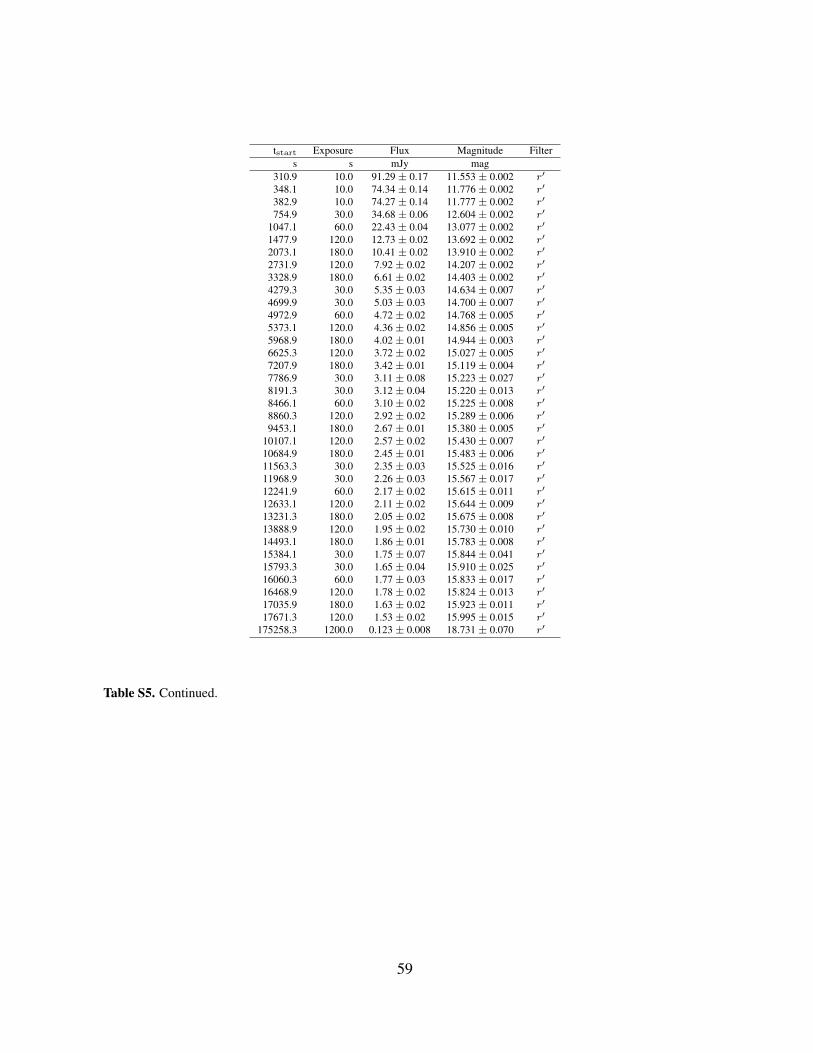
tstart Exposure Flux Magnitude Filters s mJy mag

310.9 10.0 91.29 ± 0.17 11.553 ± 0.002 r′

348.1 10.0 74.34 ± 0.14 11.776 ± 0.002 r′

382.9 10.0 74.27 ± 0.14 11.777 ± 0.002 r′

754.9 30.0 34.68 ± 0.06 12.604 ± 0.002 r′

1047.1 60.0 22.43 ± 0.04 13.077 ± 0.002 r′

1477.9 120.0 12.73 ± 0.02 13.692 ± 0.002 r′

2073.1 180.0 10.41 ± 0.02 13.910 ± 0.002 r′

2731.9 120.0 7.92 ± 0.02 14.207 ± 0.002 r′

3328.9 180.0 6.61 ± 0.02 14.403 ± 0.002 r′

4279.3 30.0 5.35 ± 0.03 14.634 ± 0.007 r′

4699.9 30.0 5.03 ± 0.03 14.700 ± 0.007 r′

4972.9 60.0 4.72 ± 0.02 14.768 ± 0.005 r′

5373.1 120.0 4.36 ± 0.02 14.856 ± 0.005 r′

5968.9 180.0 4.02 ± 0.01 14.944 ± 0.003 r′

6625.3 120.0 3.72 ± 0.02 15.027 ± 0.005 r′

7207.9 180.0 3.42 ± 0.01 15.119 ± 0.004 r′

7786.9 30.0 3.11 ± 0.08 15.223 ± 0.027 r′

8191.3 30.0 3.12 ± 0.04 15.220 ± 0.013 r′

8466.1 60.0 3.10 ± 0.02 15.225 ± 0.008 r′

8860.3 120.0 2.92 ± 0.02 15.289 ± 0.006 r′

9453.1 180.0 2.67 ± 0.01 15.380 ± 0.005 r′

10107.1 120.0 2.57 ± 0.02 15.430 ± 0.007 r′

10684.9 180.0 2.45 ± 0.01 15.483 ± 0.006 r′

11563.3 30.0 2.35 ± 0.03 15.525 ± 0.016 r′

11968.9 30.0 2.26 ± 0.03 15.567 ± 0.017 r′

12241.9 60.0 2.17 ± 0.02 15.615 ± 0.011 r′

12633.1 120.0 2.11 ± 0.02 15.644 ± 0.009 r′

13231.3 180.0 2.05 ± 0.02 15.675 ± 0.008 r′

13888.9 120.0 1.95 ± 0.02 15.730 ± 0.010 r′

14493.1 180.0 1.86 ± 0.01 15.783 ± 0.008 r′

15384.1 30.0 1.75 ± 0.07 15.844 ± 0.041 r′

15793.3 30.0 1.65 ± 0.04 15.910 ± 0.025 r′

16060.3 60.0 1.77 ± 0.03 15.833 ± 0.017 r′

16468.9 120.0 1.78 ± 0.02 15.824 ± 0.013 r′

17035.9 180.0 1.63 ± 0.02 15.923 ± 0.011 r′

17671.3 120.0 1.53 ± 0.02 15.995 ± 0.015 r′

175258.3 1200.0 0.123 ± 0.008 18.731 ± 0.070 r′

Table S5. Continued.

59

tstart Exposure Flux Magnitude Filters s mJy mag

526.3 10.0 38.22 ± 0.10 12.513 ± 0.003 V4462.9 10.0 4.50 ± 0.06 14.836 ± 0.013 V7966.3 10.0 2.39 ± 0.05 15.522 ± 0.021 V

11740.3 10.0 1.63 ± 0.04 15.941 ± 0.027 V15568.9 10.0 1.35 ± 0.05 16.145 ± 0.042 V

469.3 10.0 41.29 ± 0.15 12.622 ± 0.004 B672.1 30.0 27.40 ± 0.07 13.067 ± 0.003 B928.3 60.0 18.92 ± 0.03 13.469 ± 0.002 B

1294.9 120.0 11.96 ± 0.02 13.967 ± 0.002 B1840.3 180.0 8.36 ± 0.02 14.356 ± 0.002 B2562.1 120.0 5.56 ± 0.02 14.798 ± 0.003 B3100.9 180.0 4.89 ± 0.01 14.939 ± 0.003 B4396.3 10.0 3.83 ± 0.16 15.203 ± 0.047 B4618.9 30.0 3.52 ± 0.03 15.294 ± 0.010 B4863.1 60.0 3.41 ± 0.02 15.329 ± 0.007 B5197.3 120.0 3.36 ± 0.02 15.344 ± 0.005 B5736.1 180.0 3.00 ± 0.01 15.468 ± 0.004 B6447.1 120.0 2.61 ± 0.01 15.622 ± 0.006 B6975.1 180.0 2.51 ± 0.01 15.663 ± 0.005 B7965.1 10.0 1.98 ± 0.05 15.921 ± 0.028 B8115.1 30.0 2.12 ± 0.03 15.843 ± 0.017 B8355.1 60.0 2.09 ± 0.02 15.861 ± 0.011 B8691.1 120.0 2.16 ± 0.02 15.826 ± 0.008 B9213.1 180.0 1.88 ± 0.01 15.973 ± 0.007 B9927.1 120.0 1.83 ± 0.02 16.005 ± 0.009 B

10455.1 180.0 1.70 ± 0.01 16.086 ± 0.008 B11157.1 240.0 1.60 ± 0.01 16.154 ± 0.007 B11679.1 10.0 1.67 ± 0.05 16.107 ± 0.035 B11883.1 30.0 1.43 ± 0.03 16.276 ± 0.022 B12129.1 60.0 1.43 ± 0.02 16.272 ± 0.016 B12465.1 120.0 1.52 ± 0.02 16.210 ± 0.012 B12999.1 180.0 1.49 ± 0.01 16.224 ± 0.010 B13719.1 120.0 1.37 ± 0.02 16.318 ± 0.015 B14253.1 180.0 1.35 ± 0.02 16.337 ± 0.012 B14979.1 240.0 1.28 ± 0.02 16.389 ± 0.013 B15837.1 100.2 1.26 ± 0.03 16.409 ± 0.023 B16293.1 120.0 1.14 ± 0.03 16.520 ± 0.025 B16809.1 180.0 1.15 ± 0.02 16.513 ± 0.022 B17499.1 120.0 1.12 ± 0.03 16.539 ± 0.029 B

Table S5. Continued.

60

tstart Exposure Flux Magnitude Filters s mJy mag

146703.7 600.0 0.171 ± 0.002 18.356 ± 0.010 i′

220285.9 600.0 0.118 ± 0.002 18.759 ± 0.012 i′

393591.1 600.0 0.055 ± 0.002 19.594 ± 0.027 i′

489248.5 600.0 0.051 ± 0.001 19.664 ± 0.023 i′

578223.1 900.0 0.038 ± 0.001 19.988 ± 0.034 i′

739861.3 900.0 0.032 ± 0.001 20.175 ± 0.036 i′

829746.1 900.0 0.030 ± 0.005 20.247 ± 0.180 i′

920669.5 900.0 0.026 ± 0.010 20.400 ± 0.410 i′

1260787.3 900.0 0.028 ± 0.002 20.312 ± 0.083 i′

1435981.9 900.0 0.022 ± 0.001 20.576 ± 0.042 i′

1611121.9 900.0 0.020 ± 0.001 20.673 ± 0.054 i′

139209.1 600.0 0.148 ± 0.001 18.526 ± 0.010 r′

144618.1 600.0 0.143 ± 0.001 18.564 ± 0.012 r′

149664.1 600.0 0.131 ± 0.001 18.663 ± 0.012 r′

221105.5 600.0 0.085 ± 0.001 19.127 ± 0.011 r′

392943.7 600.0 0.046 ± 0.002 19.800 ± 0.048 r′

488596.9 600.0 0.038 ± 0.001 19.998 ± 0.020 r′

577276.3 900.0 0.032 ± 0.001 20.164 ± 0.021 r′

738914.5 900.0 0.033 ± 0.001 20.150 ± 0.026 r′

828793.3 900.0 0.030 ± 0.003 20.256 ± 0.110 r′

919716.7 900.0 0.024 ± 0.001 20.518 ± 0.029 r′

1259841.1 900.0 0.021 ± 0.001 20.631 ± 0.028 r′

1435035.7 900.0 0.028 ± 0.001 20.349 ± 0.022 r′

1610174.5 900.0 0.021 ± 0.001 20.653 ± 0.033 r′

Table S6. Liverpool telescope observation log. Magnitudes have not been corrected for Galactic absorption along

the line of sight (EB−V = 0.020 mag; (61)). The estimate extinctions in the different filters are: Ai′ = 0.040 mag,

and Ar′ = 0.052 mag. Corrected magnitudes have been converted into flux densities, Fν , following (62).

61

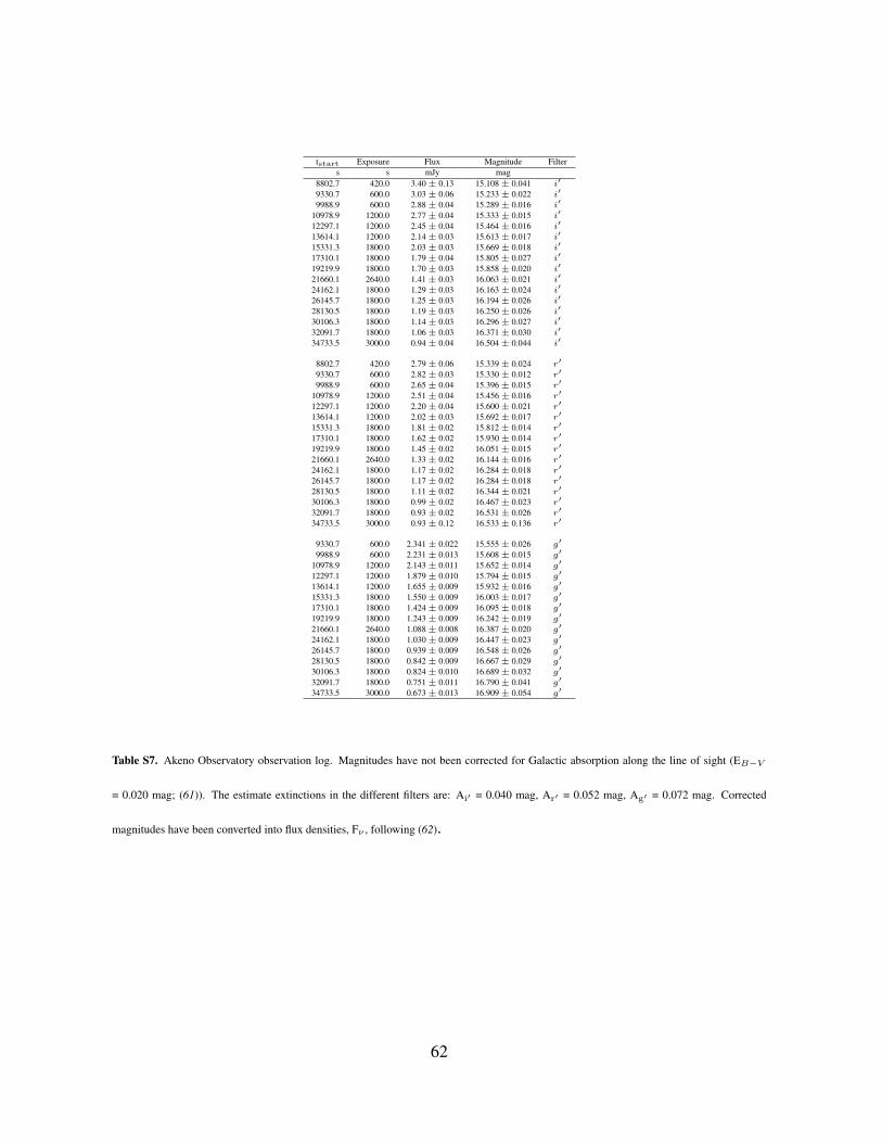
tstart Exposure Flux Magnitude Filters s mJy mag

8802.7 420.0 3.40± 0.13 15.108± 0.041 i′

9330.7 600.0 3.03± 0.06 15.233± 0.022 i′

9988.9 600.0 2.88± 0.04 15.289± 0.016 i′

10978.9 1200.0 2.77± 0.04 15.333± 0.015 i′

12297.1 1200.0 2.45± 0.04 15.464± 0.016 i′

13614.1 1200.0 2.14± 0.03 15.613± 0.017 i′

15331.3 1800.0 2.03± 0.03 15.669± 0.018 i′

17310.1 1800.0 1.79± 0.04 15.805± 0.027 i′

19219.9 1800.0 1.70± 0.03 15.858± 0.020 i′

21660.1 2640.0 1.41± 0.03 16.063± 0.021 i′

24162.1 1800.0 1.29± 0.03 16.163± 0.024 i′

26145.7 1800.0 1.25± 0.03 16.194± 0.026 i′

28130.5 1800.0 1.19± 0.03 16.250± 0.026 i′

30106.3 1800.0 1.14± 0.03 16.296± 0.027 i′

32091.7 1800.0 1.06± 0.03 16.371± 0.030 i′

34733.5 3000.0 0.94± 0.04 16.504± 0.044 i′

8802.7 420.0 2.79± 0.06 15.339± 0.024 r′

9330.7 600.0 2.82± 0.03 15.330± 0.012 r′

9988.9 600.0 2.65± 0.04 15.396± 0.015 r′

10978.9 1200.0 2.51± 0.04 15.456± 0.016 r′

12297.1 1200.0 2.20± 0.04 15.600± 0.021 r′

13614.1 1200.0 2.02± 0.03 15.692± 0.017 r′

15331.3 1800.0 1.81± 0.02 15.812± 0.014 r′

17310.1 1800.0 1.62± 0.02 15.930± 0.014 r′

19219.9 1800.0 1.45± 0.02 16.051± 0.015 r′

21660.1 2640.0 1.33± 0.02 16.144± 0.016 r′

24162.1 1800.0 1.17± 0.02 16.284± 0.018 r′

26145.7 1800.0 1.17± 0.02 16.284± 0.018 r′

28130.5 1800.0 1.11± 0.02 16.344± 0.021 r′

30106.3 1800.0 0.99± 0.02 16.467± 0.023 r′

32091.7 1800.0 0.93± 0.02 16.531± 0.026 r′

34733.5 3000.0 0.93± 0.12 16.533± 0.136 r′

9330.7 600.0 2.341± 0.022 15.555± 0.026 g′

9988.9 600.0 2.231± 0.013 15.608± 0.015 g′

10978.9 1200.0 2.143± 0.011 15.652± 0.014 g′

12297.1 1200.0 1.879± 0.010 15.794± 0.015 g′

13614.1 1200.0 1.655± 0.009 15.932± 0.016 g′

15331.3 1800.0 1.550± 0.009 16.003± 0.017 g′

17310.1 1800.0 1.424± 0.009 16.095± 0.018 g′

19219.9 1800.0 1.243± 0.009 16.242± 0.019 g′

21660.1 2640.0 1.088± 0.008 16.387± 0.020 g′

24162.1 1800.0 1.030± 0.009 16.447± 0.023 g′

26145.7 1800.0 0.939± 0.009 16.548± 0.026 g′

28130.5 1800.0 0.842± 0.009 16.667± 0.029 g′

30106.3 1800.0 0.824± 0.010 16.689± 0.032 g′

32091.7 1800.0 0.751± 0.011 16.790± 0.041 g′

34733.5 3000.0 0.673± 0.013 16.909± 0.054 g′

Table S7. Akeno Observatory observation log. Magnitudes have not been corrected for Galactic absorption along the line of sight (EB−V

= 0.020 mag; (61)). The estimate extinctions in the different filters are: Ai′ = 0.040 mag, Ar′ = 0.052 mag, Ag′ = 0.072 mag. Corrected

magnitudes have been converted into flux densities, Fν , following (62).

62

tstart Exposure Flux Magnitude Filters s mJy mag

12416.5 1800.0 2.32 ± 0.05 15.525 ± 0.023 i′

14475.1 1800.0 2.22 ± 0.05 15.570 ± 0.022 i′

16525.3 1800.0 1.94 ± 0.05 15.716 ± 0.028 i′

18576.1 1800.0 1.90 ± 0.08 15.741 ± 0.045 i′

20770.3 2040.0 1.70 ± 0.06 15.860 ± 0.042 i′

25421.5 2760.0 1.26 ± 0.04 16.188 ± 0.037 i′

28165.9 1800.0 1.11 ± 0.05 16.321 ± 0.049 i′

30216.7 1800.0 0.99 ± 0.06 16.447 ± 0.063 i′

32269.9 1800.0 0.92 ± 0.12 16.527 ± 0.147 i′

34950.1 2940.0 0.846 ± 0.054 16.619 ± 0.069 i′

12416.5 1800.0 1.93 ± 0.04 15.741 ± 0.025 r′

14475.1 1800.0 1.80 ± 0.04 15.815 ± 0.027 r′

16525.3 1800.0 1.67 ± 0.06 15.897 ± 0.042 r′

18576.1 1800.0 1.43 ± 0.03 16.064 ± 0.026 r′

20770.3 2040.0 1.42 ± 0.06 16.072 ± 0.044 r′

25421.5 2760.0 1.15 ± 0.04 16.300 ± 0.040 r′

28165.9 1800.0 1.04 ± 0.25 16.410 ± 0.264 r′

30216.7 1800.0 0.89 ± 0.05 16.581 ± 0.057 r′

32269.9 1800.0 0.84 ± 0.06 16.639 ± 0.072 r′

34950.1 2940.0 0.81 ± 0.05 16.682 ± 0.064 r′

12416.5 1800.0 1.841 ± 0.030 15.816 ± 0.045 g′

14475.1 1800.0 1.437 ± 0.027 16.085 ± 0.051 g′

16525.3 1800.0 1.326 ± 0.035 16.172 ± 0.073 g′

18576.1 1800.0 1.228 ± 0.023 16.254 ± 0.051 g′

20770.3 2040.0 1.208 ± 0.029 16.273 ± 0.067 g′

25421.5 2760.0 1.017 ± 0.022 16.460 ± 0.059 g′

28165.9 1800.0 0.847 ± 0.021 16.658 ± 0.069 g′

30216.7 1800.0 0.839 ± 0.032 16.668 ± 0.104 g′

32269.9 1800.0 0.784 ± 0.052 16.745 ± 0.181 g′

Table S8. Okayama Observatory observation log. Magnitudes have not been corrected for Galactic absorption

along the line of sight (EB−V = 0.020 mag; (61)). The estimate extinctions in the different filters are: Ai′ =

0.040 mag, Ar′ = 0.052 mag, and Ag′ = 0.072 mag. Corrected magnitudes have been converted into flux densities,

Fν , following (62).

63

tstart Exposure Flux Magnitude Filters s mJy mag

110172.1 1200.0 0.225 ± 0.012 18.057 ± 0.059 i′

112361.5 1200.0 0.220 ± 0.030 18.081 ± 0.150 i′

116807.5 1500.0 0.193 ± 0.017 18.225 ± 0.095 i′

200004.7 1800.0 0.099 ± 0.007 18.942 ± 0.079 i′

202120.3 1800.0 0.103 ± 0.008 18.906 ± 0.083 i′

205012.9 3180.0 0.103 ± 0.008 18.902 ± 0.080 i′

455880.1 540.0 0.048 ± 0.010 19.723 ± 0.219 i′

110172.1 1200.0 0.215 ± 0.007 18.123 ± 0.035 r′

112361.5 1200.0 0.192 ± 0.007 18.246 ± 0.039 r′

116807.5 1500.0 0.194 ± 0.008 18.233 ± 0.041 r′

200004.7 1800.0 0.103 ± 0.007 18.918 ± 0.059 r′

202120.3 1800.0 0.091 ± 0.006 19.059 ± 0.067 r′

205012.9 3180.0 0.090 ± 0.005 19.068 ± 0.063 r′

455880.1 540.0 0.039 ± 0.008 19.972 ± 0.226 r′

110172.1 1080.0 0.161 ± 0.002 18.453 ± 0.041 g′

112361.5 1200.0 0.153 ± 0.002 18.507 ± 0.040 g′

116807.5 1080.0 0.126 ± 0.006 18.726 ± 0.143 g′

200004.7 1800.0 0.078 ± 0.001 19.241 ± 0.052 g′

202120.3 1800.0 0.078 ± 0.002 19.250 ± 0.063 g′

205012.9 3000.0 0.075 ± 0.002 19.275 ± 0.064 g′

455880.1 540.0 0.030 ± 0.003 20.227 ± 0.232 g′

Table S9. Ishigakijima Observatory observation log. Magnitudes have not been corrected for Galactic absorption

along the line of sight (EB−V = 0.020 mag; (61)). The estimate extinctions in the different filters are: Ai′ =

0.040 mag, Ar′ = 0.052 mag, and Ag′ = 0.072 mag. Corrected magnitudes have been converted into flux densities,

Fν , following (62).

64