graphicalconstraints - umadigituma.uma.pt/bitstream/10400.13/867/1/mestradonelsonvieira.pdf ·...
TRANSCRIPT


GraphicalConstraints
A Graphical User Interface for Constraint Problems
Master's project report in Informatics Engineering
By
Nelson Manuel Marques Vieira
26th February 2015

Page 1
Author
Candidate Nelson Manuel Marques Vieira
Student Number 2098111
Email [email protected]
Project title
GraphicalConstraints, a Graphical User Interface for Constraint Problems
Advisor
Professora Doutora Elsa Cristina Bento Carvalho

Page 2
Acknowledgments
I would like to express my appreciation to all those who provided me the possibility
to complete this project. A special gratitude to my project’s advisor Professor Dr. Elsa
Carvalho, whose contribution in introducing theoretical issues of CCSP and stimulating
suggestions and encouragement throughout the project, helped me to go in the right path
to conclude the project and write this report.
A word of appreciation to Professor Dr. Jorge Cruz whose contribution and
suggestions where of decisive importance on the successful implementation of the
project.
A special thanks to my family, whose encouragement, support led me to
successfully complete the project.
I must also refer to all my professors with who I have learned so much in my
master degreed course and gave me the necessary knowledge and skills to successfully
complete this project.
Page 3
Abstract
A constraint satisfaction problem is a classical artificial intelligence paradigm
characterized by a set of variables (each variable with an associated domain of possible
values), and a set of constraints that specify relations among subsets of these variables.
Solutions are assignments of values to all variables that satisfy all the constraints.
Many real world problems may be modelled by means of constraints. The range of
problems that can use this representation is very diverse and embraces areas like
resource allocation, scheduling, timetabling or vehicle routing.
Constraint programming is a form of declarative programming in the sense that
instead of specifying a sequence of steps to execute, it relies on properties of the
solutions to be found, which are explicitly defined by constraints. The idea of constraint
programming is to solve problems by stating constraints which must be satisfied by the
solutions. Constraint programming is based on specialized constraint solvers that take
advantage of constraints to search for solutions.
The success and popularity of complex problem solving tools can be greatly
enhanced by the availability of friendly user interfaces. User interfaces cover two
fundamental areas: receiving information from the user and communicating it to the
system; and getting information from the system and deliver it to the user. Despite its
potential impact, adequate user interfaces are uncommon in constraint programming in
general.
The main goal of this project is to develop a graphical user interface that allows to,
intuitively, represent constraint satisfaction problems. The idea is to visually represent
the variables of the problem, their domains and the problem constraints and enable the
user to interact with an adequate constraint solver to process the constraints and
compute the solutions. Moreover, the graphical interface should be capable of configure
the solver’s parameters and present solutions in an appealing interactive way.
As a proof of concept, the developed application – GraphicalConstraints – focus on
continuous constraint programming, which deals with real valued variables and
numerical constraints (equations and inequalities). RealPaver, a state-of-the-art solver in
continuous domains, was used in the application. The graphical interface supports all
stages of constraint processing, from the design of the constraint network to the
presentation of the end feasible space solutions as 2D or 3D boxes.
Keywords
Constraints, Constraint programming, Continuous domains, User interfaces

Page 4
Resumo
Problemas de satisfação de restrições representam um paradigma clássico na área
de inteligência artificial, caracterizado por um conjunto de variáveis (cada variável
associada a um domínio de valores possíveis) e por um grupo de restrições que definem
relações entre subconjuntos dessas variáveis. As soluções são atribuição de valores às
variáveis que satisfazem todas as restrições.
Muitos problemas do mundo real podem ser modelados através do uso de
restrições. A diversidade de problemas que podem fazer uso desta representação é muito
grande e abrange áreas como a alocação de recursos, agendamentos, horários ou
roteamento de veículos.
Programação por restrições é uma forma de programação declarativa, pois em vez
de especificar uma sequência de passos para executar, baseia-se em propriedades das
soluções a serem encontradas, que são explicitamente definidas pelas restrições.
O objectivo da programação por restrições é resolver os problemas, declarando
restrições que devem ser satisfeitas pelas soluções. Esta é baseada em resolvedores de
restrições especializados que fazem uso das restrições para procurar as soluções.
O sucesso e popularidade das ferramentas de resolução de problemas complexos
podem ser bastante reforçados pela disponibilidade de interfaces gráficos de utilizador
fáceis de utilizar. Estas cobrem duas áreas fundamentais: receber informações do
utilizador e comunicá-la ao sistema; e obter informações do sistema e entregá-lo para o
utilizador. Apesar de seu impacto potencial, interfaces de utilizador adequados são
incomuns na programação por restrições em geral.
O principal objetivo deste projeto é desenvolver uma interface gráfica que permite,
de forma intuitiva, representar problemas de satisfação de restrições. A ideia é a de
representar visualmente as variáveis do problema, seus domínios e as restrições do
problema e permitir que o utilizador interaja com um resolvedor de restrições adequado
para processar as restrições e calcular as soluções. Além disso, a interface gráfica deve
ser capaz de configuração de parâmetros do resolvedor e de apresentação de soluções de
uma forma interactiva e amigável.
Como prova de conceito, a aplicação desenvolvida - GraphicalConstraints – foca-se
em programação restrições em domínios contínuos, e lida com variáveis reais e
restrições numéricas (equações e inequações). RealPaver, é um resolvedor state-of-the-
art em domínios contínuos e foi utilizado na aplicação. A interface gráfica suporta todos
os estágios de processamento de restrição, a partir do desenho do gráfico de restrição
para a apresentação dos resultados finais como caixas 2D ou 3D.
Keywords
Restrições Programação por restrições, Domínios Contínuos, Interfaces com
Utilizador.
Page 5
Table of contents
Acknowledgments ..................................................................................................................... 2
Abstract ..................................................................................................................................... 3
Resumo ...................................................................................................................................... 4
Table of contents ....................................................................................................................... 5
Table of figures ......................................................................................................................... 7
List of acronyms ..................................................................................................................... 10
List of abbreviations ............................................................................................................... 11
1 Introduction ................................................................................................................... 12
1.1 Goal and Contributions ................................................................................................. 14
1.2 Document Structure....................................................................................................... 14
2 State of the Art .............................................................................................................. 16
2.1 Continuous Constraint Satisfaction Problems ............................................................... 16
2.1.1 Interval Arithmetic ............................................................................ 20
2.1.2 Solving CCSPs .................................................................................. 21
2.2 Graphical User Interfaces .............................................................................................. 23
3 GraphicalConstraints Application .............................................................................. 25
3.1 Constraint Network Designer ........................................................................................ 26
3.1.1 Inserting Elements ............................................................................. 26
3.1.2 Editing and Selecting Elements......................................................... 33
3.1.3 Other functionalities .......................................................................... 37
3.1.4 Summary ........................................................................................... 39
3.2 Constraint Solver Evocation.......................................................................................... 40
3.3 Feasible Space Visualization ......................................................................................... 42
Page 6
3.3.1 Computing 2D boxes ......................................................................... 42
3.3.2 Computing 3D boxes ......................................................................... 43
3.3.3 Visualizing the feasible space box cover .......................................... 44
3.4 Examples ....................................................................................................................... 49
3.5 Technical considerations ............................................................................................... 51
3.5.1 GraphicalConstraints Installation and Execution .............................. 51
4 Conclusions and future work ....................................................................................... 52
References................................................................................................................................ 53
Appendix A .............................................................................................................................. 56
Appendix B .............................................................................................................................. 58

Page 7
Table of figures
Figure 1 - Constraint network.................................................................................. 13
Figure 2 – Graphical representation of boxes .......................................................... 14
Figure 3- Constraint Network .................................................................................. 18
Figure 4 – Intersection of circles ............................................................................. 19
Figure 5 - Box cover of the feasible space obtained through constraint reasoning . 22
Figure 6 – Branch and Prune Computation ............................................................. 23
Figure 7 – GraphicalConstraints Components ........................................................ 25
Figure 8 - CCSP represented on a constraint network ............................................ 26
Figure 9 – GraphicalConstraints main window ....................................................... 26
Figure 10 – Equality constraint a) on the shapes area; b) on the drawing area. ...... 27
Figure 11 - Popup dialog after dragging a constraint shape .................................... 27
Figure 12 – Equality Constraint dialog ................................................................... 27
Figure 13 – Inequality constraint a) on the shapes area; b) on the drawing area .... 27
Figure 14 - Inequality Constraint dialog ................................................................. 28
Figure 15 - Variable a) on the shapes area; b) on the drawing area ........................ 28
Figure 16 – Variable dialog ..................................................................................... 28
Figure 17 - Connector a) on the shapes area; b) on the drawing area ..................... 29
Figure 18 - Variable with no Connections .............................................................. 29
Figure 19 – Variable not used ................................................................................. 29
Figure 20 – Constraint connected with two variables ............................................. 30
Figure 21 – Constraint network placed in the drawing area .................................... 30
Figure 22 – Constraint network with more than one constraint .............................. 31
Figure 23 – RealPaver Grammar of Constraints ..................................................... 31
Figure 24 - GraphicalConstraints operators ............................................................ 32
Figure 25 - GraphicalConstraints Functions ............................................................ 32
Figure 26 - Constants allowed on Constraints definition ........................................ 32
Figure 27 – Edit option ............................................................................................ 33
Figure 28 – Editing inequality constraint dialog ..................................................... 33
Figure 29 – Variable editing dialog ......................................................................... 34
Figure 30 – Change variable name .......................................................................... 34
Figure 31 – Change variable name propagation ...................................................... 35
Figure 32 - Error when variable already exists ....................................................... 35
Figure 33 - Error on invalid variable name ............................................................. 35
Figure 34 – References highlight on variable y ....................................................... 36
Page 8
Figure 35 - References highlight on constraint z^2-4<=0 ....................................... 36
Figure 36 - Drop shape over existing one the change its type................................. 37
Figure 37 – Select network vertical layout .............................................................. 37
Figure 38 – Network disposed on a vertical layout ................................................. 37
Figure 39 – Save a constraint network .................................................................... 38
Figure 40 – Open a saved Constraint network ........................................................ 38
Figure 41 – Selecting a previously created network ............................................... 38
Figure 42 – Constraint network personalization ..................................................... 39
Figure 43 – Solving a CCSP defined in a Constraint Network ............................... 39
Figure 44 - Solver precision Definition ................................................................... 40
Figure 45 - .rp file containing a CCSP problem ...................................................... 41
Figure 46 – RealPaver evocation from command line interface ............................. 41
Figure 47 – RealPaver textual results ...................................................................... 41
Figure 48 - Inner boxes in dark grey and boundary boxes in light grey ................. 42
Figure 49 – Box x: [-4,0] and y:[-4.0] graphical representation ............................. 43
Figure 50 - Box x : [-0.866, 0]; y : [-0.866, 0] ; z : [-0.866, 0] graphic .................. 44
Figure 51 – Graph2D feasible space solutions ........................................................ 45
Figure 52 - Graph2D feasible space solutions with selected boxes ........................ 45
Figure 53 – Graphic 3D feasible space solutions .................................................... 46
Figure 54 – Graphic 3D feasible space solutions with 180 degrees rotation .......... 46
Figure 55 - feasible space solutions presentation options ....................................... 46
Figure 56 - Data icon ............................................................................................... 47
Figure 57 - Data table .............................................................................................. 47
Figure 58 - Sphere with all the solutions plotted ..................................................... 47
Figure 59 - Sphere with only inner solutions plotted .............................................. 48
Figure 60 - Sphere with only selected inner and boundary solutions selected ........ 48
Figure 61 - Sample2D Constraint Network ............................................................. 49
Figure 62 - Sample2D CSP Solutions Graphic ....................................................... 49
Figure 63 - Simple2DExample Constraint Network ............................................... 49
Figure 64 - Simple2DExample CSP Solutions Graphic .......................................... 50
Figure 65 – 3DSphere Constraint Network ............................................................ 50
Figure 66 - 3DSphere CSP Solutions Graphic ........................................................ 51
Figure 67 - GraphicalConstraints installed folder ................................................... 51
Figure 68 - JavaGraphicalConstraints project ......................................................... 56
Figure 69 - RealPaver C++ interface project ........................................................... 56

Page 9
Figure 70 - GraphicalConstraints folder .................................................................. 57
Figure 71 - Rpaver folder ........................................................................................ 57
Figure 72 - Software folder within RPaver ............................................................. 57

Page 10
List of definitions
Definition 1 – Constraint ......................................................................................... 16
Definition 2 - Constraint Satisfaction Problem – CSP ............................................ 17
Definition 3 - Solution of a CSP.............................................................................. 17
Definition 4 - Consistency of a CSP........................................................................ 17
Definition 5 - Constraint Network ........................................................................... 18
Definition 6 - Continuous Constraint Satisfaction Problem .................................... 18

Page 11
List of acronyms
CSP – Constraint Satisfaction Problem
CCSP – Continuous Constraint Satisfaction Problem
GUI – Graphical User Interface
CLI – Command Line Interface
Page 12
1 Introduction
Constraint Satisfaction Problems (hereafter referred as CSPs) are a classical
artificial intelligence paradigm, whose formulation is made by means of constraints.
Constraints are relations between variables that must be satisfied in order to find
solutions, which are assignments of values to variables that satisfy all the constraints
[7].
The range of values that variables can assume are the variables domains, and the
subset of such domains, that satisfy all the constraints, is the problem solution space.
This project focuses on Constraint Satisfaction Problems on Continuous Domains
(CCSPs), which are a particular kind of CSPs whose variable domains are intervals of
real numbers. In this case, the relations between variables are represented by equations
and inequalities involving the variables of the problem.
Constraint programming is a form of declarative programming. Instead of
specifying a sequence of steps to execute, it relies on properties of the solutions to be
found, which are explicitly defined by constraints. By modelling a specific problem,
when applying specific methods and algorithms to solve CSPs, a set of solutions to the
problem can be obtained.
Specialized constraint solvers are used to search for solutions that satisfy the
constraints. The usability, success and popularity of the existing solvers are greatly
enhanced by the availability of friendly user interfaces.
Graphical user interfaces are used to accommodate interaction between machines
and the human beings. User interfaces can assume on many different forms, but always
accomplish two fundamental tasks: communicating information from the system to the
user, and communicating information from the user to the system.
In this work a graphical user interface, the GraphicalConstraints tool, for an
existing constraint solver in continuous domains was developed. The graphical interface
allows the user to define variables and constraints of a given problem, set the solver
parameters and display the computed feasible space solutions. A drag and drop
approach, one of the most typical and common GUI, provides an intuitive way to draw
the elements involved in a CCSP (variables and constraints).
The developed graphical tool allows a much better perception of the problem by
supporting the design of the network of constraints. Moreover it allows to spatially
visualizing the solution space making it an appealing alternative to the classical
approaches that simply enumerate solutions textually.
The potential of graphical tool is illustrated with an example. Consider a simple
CCSP with two variables, x and y, both ranging in the interval [-4, 4] and two inequality
constraints 2 2 0.5x y xy and 0x y .
To represent this problem as an input to a constraint solver (e.g. RealPaver) a
textual file would be similar to the following:
var x in [-4.0, 4.0];
var y in [-4.0, 4.0];
x^2*y + x*y^2 - 0.5 <= 0;
x + y <= 0;

Page 13
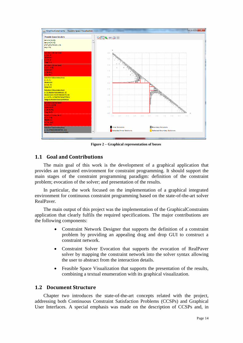
In the developed tool, this CCSP is visually represented as shown in Figure 1, after
the corresponding elements are dragged and dropped in the design area (and further
filled with the desired data).
Figure 1 - Constraint network
In addition to providing an appealing way for data introduction,
GraphicalConstraints also allows an immediate visual perception of the relationship
between constraints and variables, comparatively to a textual representation. The more
complex the problem, the more apparent this becomes.
A traditional constraint solver would produce a file with (possibly) hundreds or
thousands of solutions (depending on the precision required) and the feasible space
solutions would be given in a format similar to the following:
Solution 1 (inner box)
x : [-4, 0]
y : [-4, 0]
Solution 2 (inner box)
x : [-1, -0.5]
y : [0, 0.5]
Solution 3 (boundary box)
x : <1, 1>
y : <-4, -4>
Solution 4 (boundary box)
x : [2.982667025389525, 3]
y : [-3.75, -3.706792743477501]
In GraphicalConstraints, these solutions are visually represented as observed in
Figure 2.
Having only textual solution descriptions it is not clear how to spatially interpret
the obtained solutions, especially when there are hundreds or thousands of them.
Graphical results give a complementary picture of the solution space and enable to
select a specific textual solution description identifying it in the solution space (by
marking it with a different colour).
Page 14
Figure 2 – Graphical representation of boxes
1.1 Goal and Contributions
The main goal of this work is the development of a graphical application that
provides an integrated environment for constraint programming. It should support the
main stages of the constraint programming paradigm: definition of the constraint
problem; evocation of the solver; and presentation of the results.
In particular, the work focused on the implementation of a graphical integrated
environment for continuous constraint programming based on the state-of-the-art solver
RealPaver.
The main output of this project was the implementation of the GraphicalConstraints
application that clearly fulfils the required specifications. The major contributions are
the following components:
Constraint Network Designer that supports the definition of a constraint
problem by providing an appealing drag and drop GUI to construct a
constraint network.
Constraint Solver Evocation that supports the evocation of RealPaver
solver by mapping the constraint network into the solver syntax allowing
the user to abstract from the interaction details.
Feasible Space Visualization that supports the presentation of the results,
combining a textual enumeration with its graphical visualization.
1.2 Document Structure
Chapter two introduces the state-of-the-art concepts related with the project,
addressing both Continuous Constraint Satisfaction Problems (CCSPs) and Graphical
User Interfaces. A special emphasis was made on the description of CCSPs and, in

Page 15
particular on interval arithmetic and on constraint propagation. The goal is to present the
reader with some introductory notes about the subject so that a context of the project
scope may be understood. Complementary, some theoretical considerations about
graphical user interfaces and their importance nowadays when dealing with computer
systems and human-machine interfaces were also addressed.
Chapter three describes the GraphicalConstraints application explaining, in detail,
its component tools: the Constraint Network Designer; the Constraint Solver Evocation;
and the Feasible Space Visualization.
The last chapter presents the main conclusions and discusses directions for future
work.

Page 16
2 State of the Art
2.1 Continuous Constraint Satisfaction Problems
Constraint satisfaction problems were introduced in the 1970s (see, for example,
[6]. This area is subject to intense research in both artificial intelligence and operations
research. The regularity in its formulation provides a common basis to analyse and
solve problems of many application areas. It has been successfully applied in a diverse
number of fields including molecular biology, electrical engineering, operations
research and numerical analysis [16].
In generic terms, constraint satisfaction is the process of finding a solution to a set
of constraints that impose conditions that variables must satisfy. A solution is therefore
a set of values that can be assigned to the variables that satisfies all constraints. For
example, a car engine cannot exceed the size the space in which it fits, yet it cannot
produce less than a specified horse power [9]. In this example we have a constraint
satisfaction problem on two variables – engine size and engine horse power, which are
subject to two constraints - or conditions that must be satisfied.
A constraint satisfaction problem is therefore a mathematical model with
constraints and the goal of constraint solving is to find a feasible solution (or solutions).
In computer science, CSPs are handled or solved by constraint programming
techniques. Constraint programming has already been successfully applied in numerous
domains of human knowledge [16], including:
Interactive graphic systems (to express geometric coherence in the case of scene
analysis);
Operations research problems (various optimization problems, in particular
scheduling problems);
Molecular biology (DNA sequencing, construction of 3D models of proteins);
Business applications (option trading);
Electrical engineering (location of faults in the circuits, computing the circuit
layouts, testing and verification of circuits design);
Numerical computation (solving polynomial constraints with guaranteed
precision);
Natural language processing (construction of efficient parsers);
Computer algebra (solving and/or simplifying equations over various algebraic
structures).
We will now formalize some definitions related with Constraint Satisfaction
Problems. The following is the formal definition of a constraint [11].
Definition 1 – Constraint
A constraint c is a pair (s, p), where s is a tuple of m variables1 2( , , , )mv v v , the
constraint scope, and p is a relation of arity m, the constraint relation. The relation p is
a subset of the set of all m-tuples of elements from the Cartesian product
1 2 .... mD D D where iD is the domain of the variable vi:
1, 2 1 1 2 2{( , , ) | , , , }m m mp d d d d D d D d D
Page 17
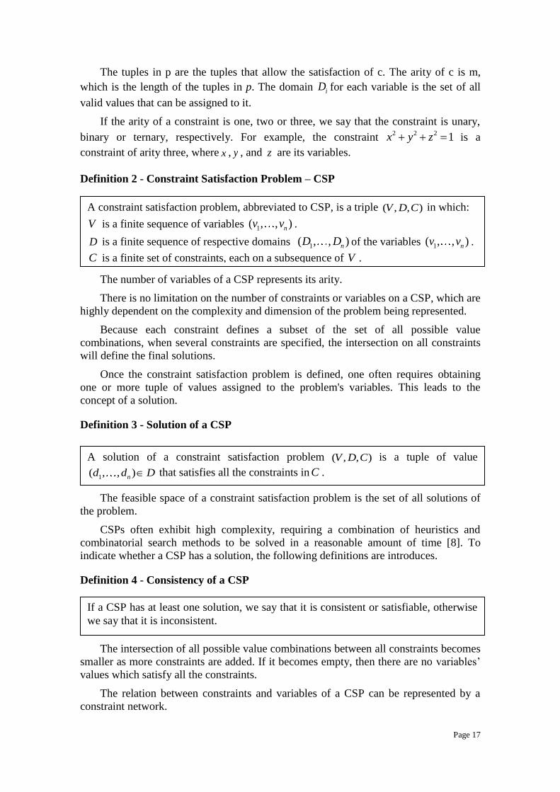
The tuples in p are the tuples that allow the satisfaction of c. The arity of c is m,
which is the length of the tuples in p. The domain iD for each variable is the set of all
valid values that can be assigned to it.
If the arity of a constraint is one, two or three, we say that the constraint is unary,
binary or ternary, respectively. For example, the constraint 2 2 2 1x y z is a
constraint of arity three, where x , y , and z are its variables.
Definition 2 - Constraint Satisfaction Problem – CSP
The number of variables of a CSP represents its arity.
There is no limitation on the number of constraints or variables on a CSP, which are
highly dependent on the complexity and dimension of the problem being represented.
Because each constraint defines a subset of the set of all possible value
combinations, when several constraints are specified, the intersection on all constraints
will define the final solutions.
Once the constraint satisfaction problem is defined, one often requires obtaining
one or more tuple of values assigned to the problem's variables. This leads to the
concept of a solution.
Definition 3 - Solution of a CSP
The feasible space of a constraint satisfaction problem is the set of all solutions of
the problem.
CSPs often exhibit high complexity, requiring a combination of heuristics and
combinatorial search methods to be solved in a reasonable amount of time [8]. To
indicate whether a CSP has a solution, the following definitions are introduces.
Definition 4 - Consistency of a CSP
The intersection of all possible value combinations between all constraints becomes
smaller as more constraints are added. If it becomes empty, then there are no variables’
values which satisfy all the constraints.
The relation between constraints and variables of a CSP can be represented by a
constraint network.
A constraint satisfaction problem, abbreviated to CSP, is a triple ( , , )V D C in which:
V is a finite sequence of variables 1( , , )nv v .
D is a finite sequence of respective domains 1( , , )nD D of the variables 1( , , )nv v .
C is a finite set of constraints, each on a subsequence of V .
A solution of a constraint satisfaction problem ( , , )V D C is a tuple of value
1( , , )nd d D that satisfies all the constraints in C .
If a CSP has at least one solution, we say that it is consistent or satisfiable, otherwise
we say that it is inconsistent.

Page 18
Definition 5 - Constraint Network
Figure 3 illustrates a constraint network with 5 variables and 9 constraints.
Figure 3- Constraint Network
This work deals with Continuous Constraint Satisfaction Problems (CCSPs). A
CCSP uses variables whose domains are built on intervals of real numbers, i.e.
continuous domains. A continuous domain is a connected set of real numbers, e.g. a real
interval. For example, the interval [1,5] is a continuous domain, containing all the real
numbers between 1 and 5.
Example: The domain 1 1, 3, 5, 7D is a discrete domain. The domains
2D 10,20 , 3D 3,25 or 4D ] ,10] are connected sets of real numbers, and
therefore continuous domains.
Conversely, the domain 5D 2, 4 [5,7] is not a connected set of real numbers,
and for that reason is not a continuous domain. However, it is the union of two
continuous domains.
Definition 6 - Continuous Constraint Satisfaction Problem
In the literature, CCSPs are sometimes referred to as numerical CSPs.
Example: Consider the CCSP with constraint 2 2 1x y where [ 2,4]x and
[ 4,2]y . Its solution set is the unit circle centred at the origin of the coordinate
system.
A constraint network is a graph, with: one node for every variable (drawn as a circle);
one node for every constraint (drawn as a rectangle); undirected edges between
variable nodes and constraint nodes, whenever a given variable is involved in a given
constraint.
A continuous constraint satisfaction problem, abbreviated to CCSP or Continuous
CSP, is a constraint satisfaction problem ( , , )V D C where all domains in D are
continuous.

Page 19
Example: Consider the CCSP with constraint 2 2 1x y where [ 2,4]x and
[ 4,2]y . Its solution set is the unit circumference centred at the origin of the
coordinate system.
Example: Consider the CCSP with constraints 2 2 1x y and
2y a x where
[ 2,4]x and [ 4,2]y . If a = 1, the solution set is the set of three points
( 1,0),(0, 1) and (1,0) . If a = 4, the solution set is empty.
Example: Consider the problem described as follows [13]:
Given a real number 0d and a circle with centre 0( , )ox y and radius r , find all
the points on the circle whose distance to the origin is d .
As shown in Figure 4, this is a problem of intersection of circles.
Figure 4 – Intersection of circles
In this problem, we are able to identify the following data:
4 constants: d , 0x , 0y , r . Depending on their values, the problem has 0, 1 or
2 solutions.
2 variables: the coordinates ( x ; y ) of the point. Since these variables lie a
priori in the variable domains are defined as the set .
2 constraints:
( , )x y is required to be on the given circumference:
2 2 2
0 0( ) ( )r x x y y
The distance of ( , )x y to the origin is d :
2 2 2d x y
2 domains (the set ):
] , [x
] , [y
The above examples show that, in general, the solution set of a CCSP can be empty,
isolated points, a surface, or a volume.
Since the variable domains in CCSPs are continuous, the classic techniques for
solving CSPs with discrete domains cannot apply. In general, solving a CCSP by simply

Page 20
discretizing its variable domains and then using classic techniques for CSPs with
discrete domains are usually inefficient. Interval arithmetic techniques are used to deal
with CCSP solving process.
2.1.1 Interval Arithmetic
Being associated to intervals, CSPs on continuous domains relates directly to
interval arithmetic, which is an extension of real arithmetic for real intervals. Interval
analysis [12] that relates to interval arithmetic is used in CCSP in order to eliminate
inconsistent solutions, and to guarantee the soundness of constraint propagation
techniques.
This section presents a short introduction on interval arithmetic. More details can
be found in the following fundamental books: introduction to interval computation [23,
12], fundamental interval methods for systems of equations [23]; some recently added
applications [24], and extended interval methods for optimization problems [25].
Interval analysis was developed by mathematicians since the late 1950’s as an
approach on bounding rounding and measurement errors in mathematical computations
and thus developing numerical methods that yield reliable results.
It represents each value as a range of possibilities. For example, instead of
estimating the someone’s height using standard arithmetic as 2.0 meters, using interval
arithmetic we are certain that such person is somewhere between 1.97 and 2.03 meters
height [11]. It means that the person’s height can be any of the values within the interval[1.97,2.03]
A real interval is a set of real numbers having the property that numbers that are
enclosed between any two numbers in the set is also included in complete the set. The
interval of numbers between a and b, including a and b, is denoted [a, b] (in this work
we only consider closed intervals):
[ , ] { | }a b r a r b
If a = b the interval is degenerated and is represented as .
The generalization of intervals to several dimensions is of relevance in this work.
An n-dimensional box B is the Cartesian product of n intervals and is denoted by
1 nI I , where each Ii is an interval.
Elementary set operations, such as ∩ (intersection), ∪ (union), (inclusion) are
valid for intervals. While the intersection between two intervals is still an interval, this
is not the case with the union of two disjoint intervals, where the result is a set that
cannot be represented exactly by a single interval.
Interval arithmetic defines a set of operations on intervals, and is an extension of
real arithmetic for intervals. The obtained interval is the set of all the values that result
from a point-wise evaluation of the arithmetic operator on all the values of the operands.
In the case of the four elementary operations for interval arithmetic, if I1 and I2 are
two real intervals (with 20 I ):
1 2 1 2 { | , }, { , , , }I I x y x I y I
The previous set definition characterizes these operations mathematically; the
benefit of interval arithmetic is due to the operational definitions based on the interval

Page 21
bounds (a short description can be found in [25]). For example, let x [ , ]x x and
y [ , ]y y be two closed intervals, the elementary operator definition based on the
interval bounds are:
x+y [ , ]x y x y
x-y [ , ]x y x y
x y [min{ , , , },max{ , , , }]xy xy xy xy xy xy xy xy
x y x 1/ y if 0 y, where 1/y [min(1/ ,1/ ),max(1/ ,1/ )]y y y y
Note that the division is not defined in standard interval arithmetic when
denominator contains zero. In this case, one often assumes the result is the universal
interval [−∞, +∞], for convenience and safety. Simple arithmetic expressions are
composed of these four fundamental operations.
In order to represent a continuous domain in a computer system, F-numbers are
used [11]. F-numbers are introduced because there are infinite numbers on an interval,
and not all are machine representable - machines are restricted to represent a finite set of
elements. Computers use a floating point system for representing real numbers, whose
elements are a finite subset, F, of the reals, the F-numbers. This subset includes the real
number zero (0) as well as the infinity symbols and (which are not reals).
An F-interval is a real interval bounded by F-numbers. An n-dimensional F-box is
the Cartesian product of n F-intervals.
2.1.2 Solving CCSPs
Constraint reasoning aims to eliminate values from the initial search space (the
Cartesian product of all variable domains) that do not satisfy the constraints. It is done
by subdividing the search space and pruning the solutions until a stopping criterion is
satisfied in a process called branch and prune. Branching process divides the search
space into smaller areas and pruning process eliminates all sets of values that are proved
to be inconsistent [27].
To eliminate incompatible values on a particular constraint, safe narrowing
operators (mappings between boxes) are associated with the constraint. These must be
correct in order not to eliminate valid solutions and contracting, which means that the
obtained box is contained in the original. To guarantee such properties interval analysis
methods are used.
As an example, consider the following constraint: x y z
Interval narrowing operators can be associated with the constraint to prune the
domain of each variable:
X X Z Y, Y Y Z X, Z Z X Y
If, for instance, the domains of the variables are X [1,3] , Y [3,7] and Z [0,5] ,
narrowing operators can be used to prune them to:

Page 22
X [1,3] [0,5] [3,7] = [1,3] [ 7,2] [1,2]
Y [3,7] [0,5] [1,2] = [3,7] [ 2,4] [3,4]
Z [0,5] [1,2] [3,7] = [0,5] [4,9] [4,5]
Using this technique, which is based on interval arithmetic, safe narrowing
operators are able to reduce the original box 1,3 3,7 0,5 into 1,2 3,4 4,5
with the guarantee that no solution is lost.
Once narrowing operators are associated with all the constraints, pruning can be
done through constraint propagation. Narrowing operators associated with a constraint
remove some incompatible values from the variables domain and then this removal is
propagated to all the constraints with common variables. Constraint propagation ends
when a fixed point is reached, meaning that domains cannot be further reduced by any
narrowing operator.
Pruning through constraint propagation is highly dependent on narrowing operators
ability for discarding inconsistent values [30]. Further pruning is usually done by
splitting the resulting domains and reapplying constraint propagation to each sub-
domain. Continuous constraint reasoning will eventually terminate due to the imposition
of conditions on the branching process (e.g. small enough domains are not considered
for branching) [27].
No solution is lost during the branch-and-prune process. Constraint reasoning
provides a safe method for computing an enclosure of the feasible space of a CCSP. It
applies branch and prune steps to reshape the initial search space (a box) maintaining a
set of working boxes (a box cover) throughout the process. Some of the boxes may be
classified as inner boxes, if it can be proved that they are contained in the feasible space
(again interval analysis techniques are used to guarantee that all constraints are
satisfied) [27].
Example: Figure 5 illustrates solutions achieved through continuous constraint
reasoning for a CCSP with two variables x and y, ranging within [-,], and with one
constraint: 2 2 0.5x y xy
Figure 5 - Box cover of the feasible space obtained through constraint reasoning
Constraint reasoning can prove that there are regions with no solutions (white) and
identify regions where every point is a solution, identifying dark grey areas. Those are
called inner boxes.
Page 23
Some boxes cannot be proved to contain solutions and are painted in light grey.
They are called boundary boxes, and represent the uncertainty on the feasible space
enclosure. It may be further reduced by branching and pruning.
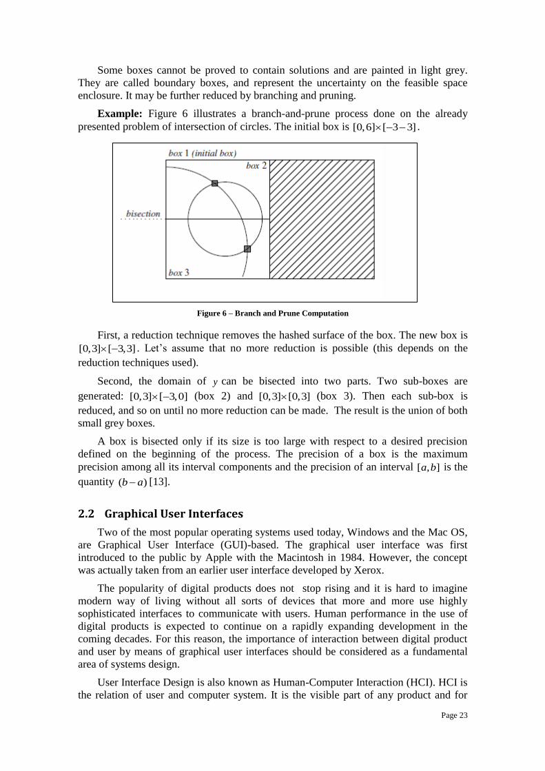
Example: Figure 6 illustrates a branch-and-prune process done on the already
presented problem of intersection of circles. The initial box is [0,6] [ 3 3] .
Figure 6 – Branch and Prune Computation
First, a reduction technique removes the hashed surface of the box. The new box is
[0,3] [ 3,3] . Let’s assume that no more reduction is possible (this depends on the
reduction techniques used).
Second, the domain of y can be bisected into two parts. Two sub-boxes are
generated: [0,3] [ 3,0] (box 2) and [0,3] [0,3] (box 3). Then each sub-box is
reduced, and so on until no more reduction can be made. The result is the union of both
small grey boxes.
A box is bisected only if its size is too large with respect to a desired precision
defined on the beginning of the process. The precision of a box is the maximum
precision among all its interval components and the precision of an interval [ , ]a b is the
quantity ( )b a [13].
2.2 Graphical User Interfaces
Two of the most popular operating systems used today, Windows and the Mac OS,
are Graphical User Interface (GUI)-based. The graphical user interface was first
introduced to the public by Apple with the Macintosh in 1984. However, the concept
was actually taken from an earlier user interface developed by Xerox.
The popularity of digital products does not stop rising and it is hard to imagine
modern way of living without all sorts of devices that more and more use highly
sophisticated interfaces to communicate with users. Human performance in the use of
digital products is expected to continue on a rapidly expanding development in the
coming decades. For this reason, the importance of interaction between digital product
and user by means of graphical user interfaces should be considered as a fundamental
area of systems design.
User Interface Design is also known as Human-Computer Interaction (HCI). HCI is
the relation of user and computer system. It is the visible part of any product and for

Page 24
that reason the importance of good user interface design can be the difference between
product acceptance and rejection.
User interfaces can assume many different forms, but independently on their form,
they are built to accomplish two main objectives: communicating information from the
system to the user, and communicating information from the user to the system.
If end-users feel it is hard to learn, hard to use, or too cumbersome, a potential
excellent product could collapse. That’s why good user interface design makes a
product easy to understand and use, which results in greater user acceptance.
To get best interaction between the product and the users, the graphical user
interface design needs to have some design values and requires a systematic approach to
the design process [17]. Optimum performance requires a model of interaction to
understand exactly what is going on in the interaction and identify the likely root of
difficulties that are due to arise [17].
To achieve the successful interaction of user and product, there are some principles
that should be considered. The reader can find more detail in [28]. There is already
research made that provide a guide for well-designed digital product by giving some
fundamentals about graphical user interface. [17]. Theoretical insights into cognitive
architecture emphasize the memory and attentional constraints of humans.
These lessons have been studied and learned by the HCI experts who claim that
interaction sequences should be designed to minimize short term memory load and for
that reason, not demanding a user choose from an excessive number of menu items or
requiring to remember numbers or characters from one screen to another, etc.
Since recognition memory is superior to absolute recall, the use of menus is now
the norm in design compared to the command line interfaces of the 1980s, which are
outdated and required users to memorize control arguments.
If we put two application experts side by side, one equipped with the GUI and the
other with the command line interface (CLI), the CLI user can be much faster than the
graphical user interface operator. In fact CLI does not use computer processor to draw
GUI and CLI does not provide feedback unless you do things the wrong way. But the
cognitive load still is on the CLI operator - he needs to know exactly what to type and
may also need be more skilled than a GUI operator.
Page 25
3 GraphicalConstraints Application
The project goal, as enunciated in the project proposal is to develop a graphical
user interface on a constraint solver in continuous domains. The developed application
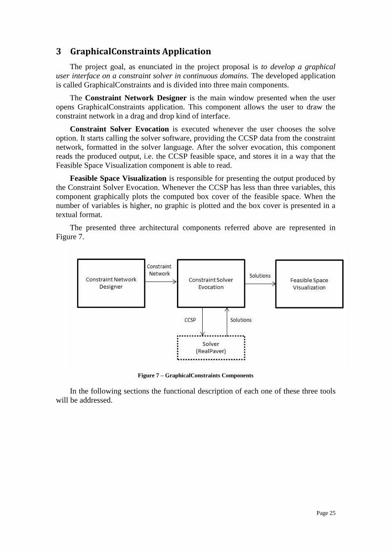
is called GraphicalConstraints and is divided into three main components.
The Constraint Network Designer is the main window presented when the user
opens GraphicalConstraints application. This component allows the user to draw the
constraint network in a drag and drop kind of interface.
Constraint Solver Evocation is executed whenever the user chooses the solve
option. It starts calling the solver software, providing the CCSP data from the constraint
network, formatted in the solver language. After the solver evocation, this component
reads the produced output, i.e. the CCSP feasible space, and stores it in a way that the
Feasible Space Visualization component is able to read.
Feasible Space Visualization is responsible for presenting the output produced by
the Constraint Solver Evocation. Whenever the CCSP has less than three variables, this
component graphically plots the computed box cover of the feasible space. When the
number of variables is higher, no graphic is plotted and the box cover is presented in a
textual format.
The presented three architectural components referred above are represented in
Figure 7.
Figure 7 – GraphicalConstraints Components
In the following sections the functional description of each one of these three tools
will be addressed.
Page 26
3.1 Constraint Network Designer
The Constraint Network Designer tool allows the user to draw the constraint
network in a drag and drop kind of interface. It is opened when the user chooses the
GraphicalConstraints application.
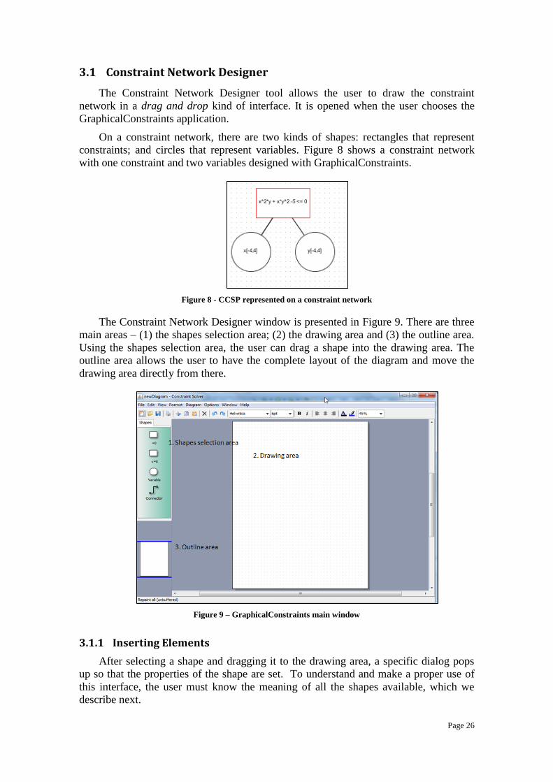
On a constraint network, there are two kinds of shapes: rectangles that represent
constraints; and circles that represent variables. Figure 8 shows a constraint network
with one constraint and two variables designed with GraphicalConstraints.
Figure 8 - CCSP represented on a constraint network
The Constraint Network Designer window is presented in Figure 9. There are three
main areas – (1) the shapes selection area; (2) the drawing area and (3) the outline area.
Using the shapes selection area, the user can drag a shape into the drawing area. The
outline area allows the user to have the complete layout of the diagram and move the
drawing area directly from there.
Figure 9 – GraphicalConstraints main window
3.1.1 Inserting Elements
After selecting a shape and dragging it to the drawing area, a specific dialog pops
up so that the properties of the shape are set. To understand and make a proper use of
this interface, the user must know the meaning of all the shapes available, which we
describe next.

Page 27
Equality constraint: An equality constraint is represented by a rectangle as shown
in Figure 10 a). This shape allows the user to insert equality constraints. For example:
x^2*y + x*y^2 = 0;
When placed in the drawing area, the equality constraint is shown with a black
border, as shown in Figure 10 b).
a) b)
Figure 10 – Equality constraint a) on the shapes area; b) on the drawing area.
After selecting the insertion of an equality constraint (as shown in the red square on
the left of Figure 11) a popup dialog is presented (right side of Figure 11 and Figure
12).
Figure 11 - Popup dialog after dragging a constraint shape
Figure 12 – Equality Constraint dialog
Inequality constraint: An equality constraint is represented by a rectangle as
shown in Figure 13 a). This shape allows the user to insert inequality constraints. For
example:
x^2*y + x*y^2 - 0.5 <= 0;
When placed in the drawing area, the inequality constraint is shown with a red
border, as can be observed in Figure 13 b).
a) b)
Figure 13 – Inequality constraint a) on the shapes area; b) on the drawing area
Page 28
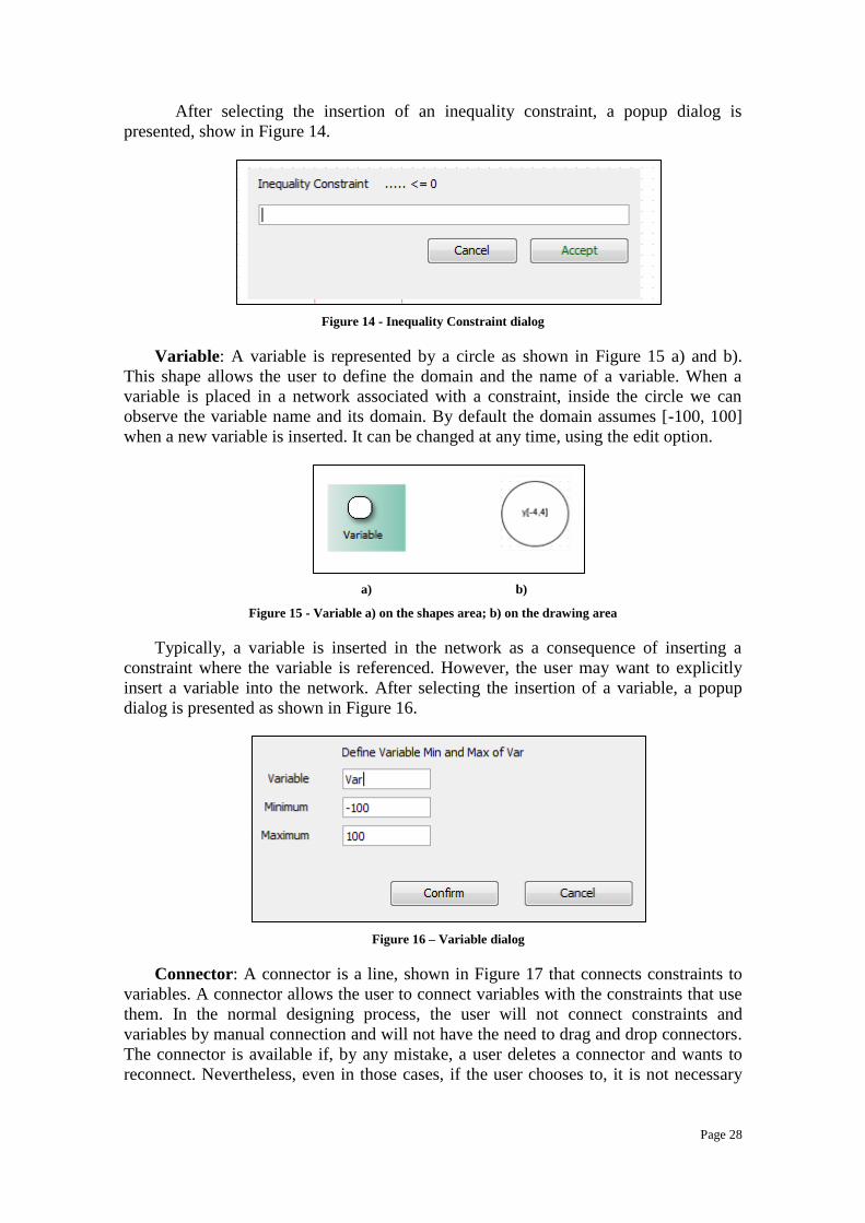
After selecting the insertion of an inequality constraint, a popup dialog is
presented, show in Figure 14.
Figure 14 - Inequality Constraint dialog
Variable: A variable is represented by a circle as shown in Figure 15 a) and b).
This shape allows the user to define the domain and the name of a variable. When a
variable is placed in a network associated with a constraint, inside the circle we can
observe the variable name and its domain. By default the domain assumes [-100, 100]
when a new variable is inserted. It can be changed at any time, using the edit option.
a) b)
Figure 15 - Variable a) on the shapes area; b) on the drawing area
Typically, a variable is inserted in the network as a consequence of inserting a
constraint where the variable is referenced. However, the user may want to explicitly
insert a variable into the network. After selecting the insertion of a variable, a popup
dialog is presented as shown in Figure 16.
Figure 16 – Variable dialog
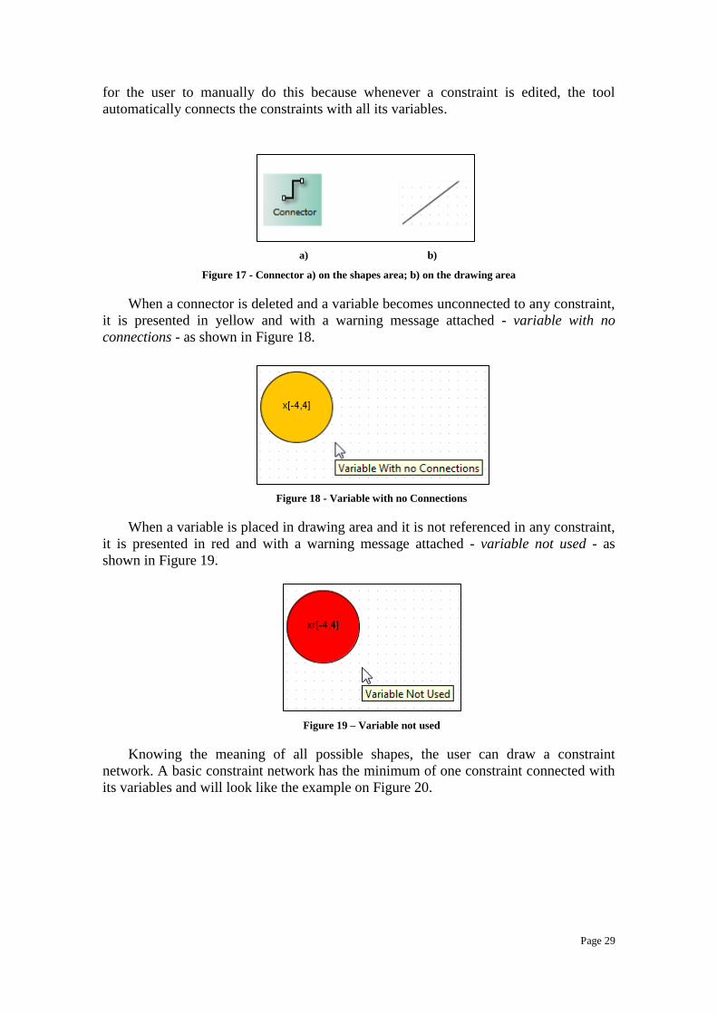
Connector: A connector is a line, shown in Figure 17 that connects constraints to
variables. A connector allows the user to connect variables with the constraints that use
them. In the normal designing process, the user will not connect constraints and
variables by manual connection and will not have the need to drag and drop connectors.
The connector is available if, by any mistake, a user deletes a connector and wants to
reconnect. Nevertheless, even in those cases, if the user chooses to, it is not necessary
Page 29
for the user to manually do this because whenever a constraint is edited, the tool
automatically connects the constraints with all its variables.
a) b)
Figure 17 - Connector a) on the shapes area; b) on the drawing area
When a connector is deleted and a variable becomes unconnected to any constraint,
it is presented in yellow and with a warning message attached - variable with no
connections - as shown in Figure 18.
Figure 18 - Variable with no Connections
When a variable is placed in drawing area and it is not referenced in any constraint,
it is presented in red and with a warning message attached - variable not used - as
shown in Figure 19.
Figure 19 – Variable not used
Knowing the meaning of all possible shapes, the user can draw a constraint
network. A basic constraint network has the minimum of one constraint connected with
its variables and will look like the example on Figure 20.

Page 30
Figure 20 – Constraint connected with two variables
To draw a network, the user places the constraint in any place of the drawing area.
After filling the constraint dialog, the constraint network is placed in the drawing area,
on the spot where the user released it, representing the constraint inserted and the
variables associated (as can be observed in Figure 21).
Figure 21 – Constraint network placed in the drawing area
New constraints can be added to the network. These are automatically placed in the
existing network and all the variables connected. If the new constraint references
variables that already exist in the network, the connection is made to those variables. If
a new variable is detected (ahead in this chapter there is an explanation of how variables
are recognized in the constraint formula), then it is automatically inserted as a new
variable in the network. Figure 22 shows a network with more than one constraint
defined.

Page 31
Figure 22 – Constraint network with more than one constraint
Constraints are inserted in a free format field. It gives the user the freedom to insert
any constraint without format restrictions. To interpret the constraint, regular
expressions were coded in the application, with the purpose of interpretation and
splitting the constraint into components. The regular expression interpretation takes into
account that a constraint is an equation or inequality involving numbers, constants,
variables and function symbols [20]. These can by identified by patterns in regular
expressions and then split into components. As an example, the complete grammar
admitted by RealPaver is as follows in Figure 23.
Figure 23 – RealPaver Grammar of Constraints
Variables are detected as patterns starting with a letter and followed by letters or
numbers. Examples of variable names are: x; x1, variable.
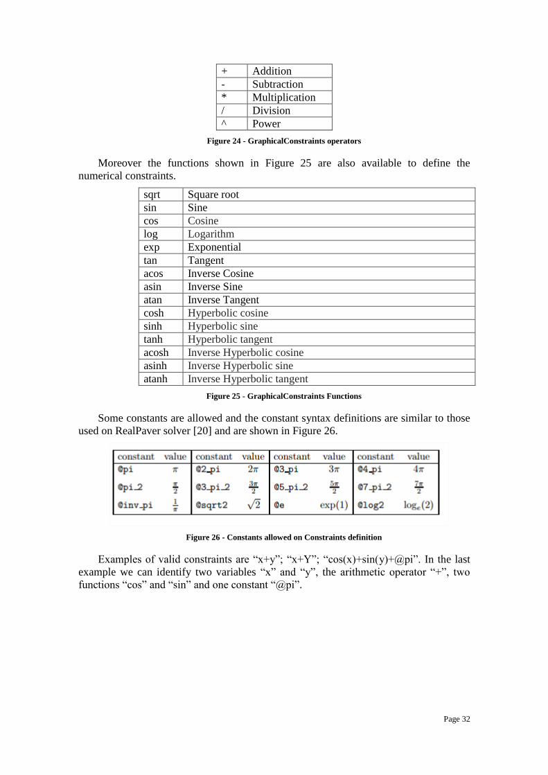
In addition to variables, arithmetic operators can also be defined. The usual
arithmetic operators are available as shown in Figure 24.
Page 32
+ Addition
- Subtraction
* Multiplication
/ Division
^ Power
Figure 24 - GraphicalConstraints operators
Moreover the functions shown in Figure 25 are also available to define the
numerical constraints.
sqrt Square root
sin Sine
cos Cosine
log Logarithm
exp Exponential
tan Tangent
acos Inverse Cosine
asin Inverse Sine
atan Inverse Tangent
cosh Hyperbolic cosine
sinh Hyperbolic sine
tanh Hyperbolic tangent
acosh Inverse Hyperbolic cosine
asinh Inverse Hyperbolic sine
atanh Inverse Hyperbolic tangent
Figure 25 - GraphicalConstraints Functions
Some constants are allowed and the constant syntax definitions are similar to those
used on RealPaver solver [20] and are shown in Figure 26.
Figure 26 - Constants allowed on Constraints definition
Examples of valid constraints are “x+y”; “x+Y”; “cos(x)+sin(y)+@pi”. In the last
example we can identify two variables “x” and “y”, the arithmetic operator “+”, two
functions “cos” and “sin” and one constant “@pi”.
Page 33
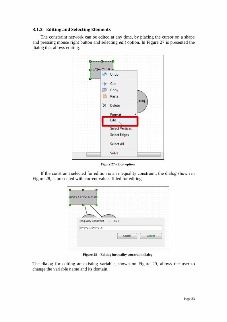
3.1.2 Editing and Selecting Elements
The constraint network can be edited at any time, by placing the cursor on a shape
and pressing mouse right button and selecting edit option. In Figure 27 is presented the
dialog that allows editing.
Figure 27 – Edit option
If the constraint selected for edition is an inequality constraint, the dialog shown in
Figure 28, is presented with current values filled for editing.
Figure 28 – Editing inequality constraint dialog
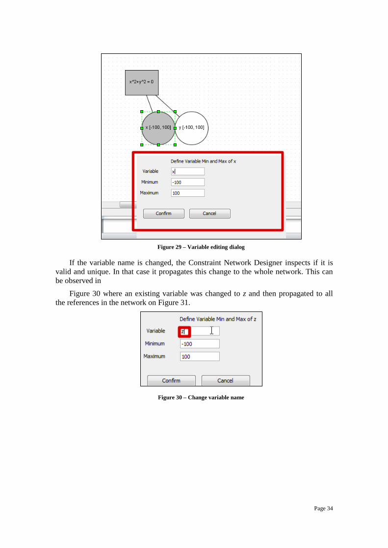
The dialog for editing an existing variable, shown on Figure 29, allows the user to
change the variable name and its domain.
Page 34
Figure 29 – Variable editing dialog
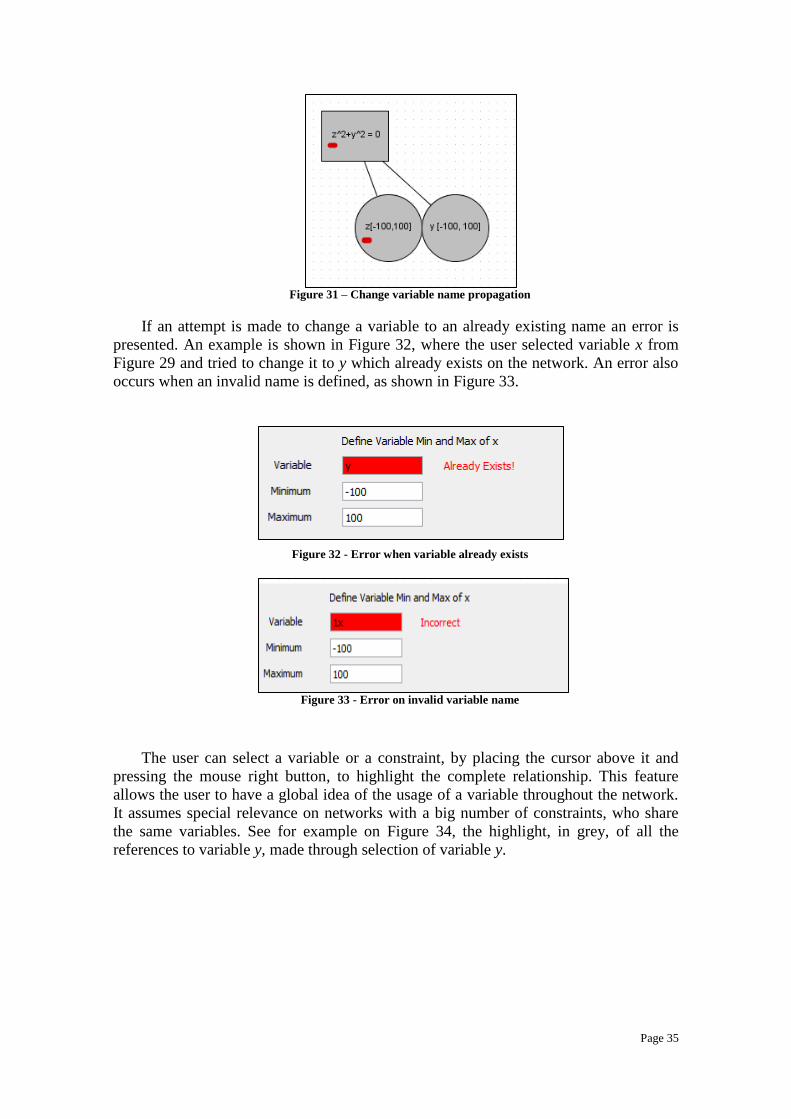
If the variable name is changed, the Constraint Network Designer inspects if it is
valid and unique. In that case it propagates this change to the whole network. This can
be observed in
Figure 30 where an existing variable was changed to z and then propagated to all
the references in the network on Figure 31.
Figure 30 – Change variable name
Page 35
Figure 31 – Change variable name propagation
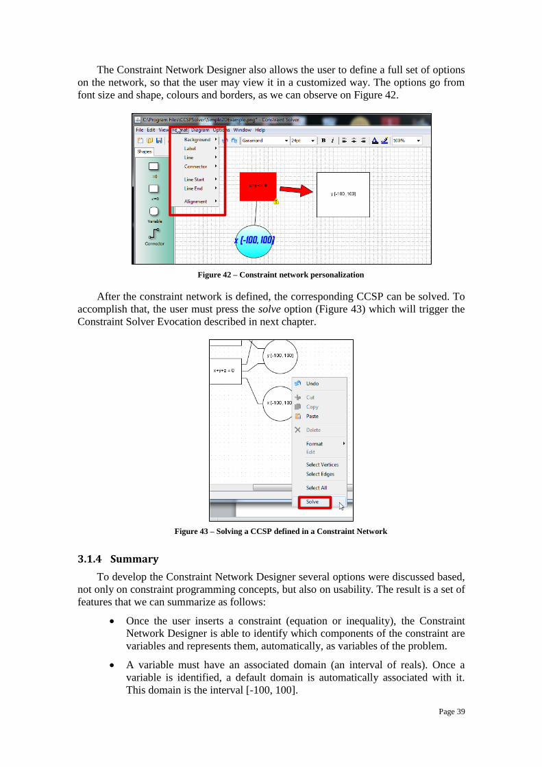
If an attempt is made to change a variable to an already existing name an error is
presented. An example is shown in Figure 32, where the user selected variable x from
Figure 29 and tried to change it to y which already exists on the network. An error also
occurs when an invalid name is defined, as shown in Figure 33.
Figure 32 - Error when variable already exists
Figure 33 - Error on invalid variable name
The user can select a variable or a constraint, by placing the cursor above it and
pressing the mouse right button, to highlight the complete relationship. This feature
allows the user to have a global idea of the usage of a variable throughout the network.
It assumes special relevance on networks with a big number of constraints, who share
the same variables. See for example on Figure 34, the highlight, in grey, of all the
references to variable y, made through selection of variable y.

Page 36
Figure 34 – References highlight on variable y
Figure 35 shows that the selection of constraint z^2-4 <=0, highlights variable z
and constraint z^2+y^2=0, that shares a common variable z.
Figure 35 - References highlight on constraint z^2-4<=0
If an equality constraint needs to be changed to equality or vice versa, the user may
drag and drop the new shape over the existing one and edit to correct its content. In
Figure 36, is presented a case where an equality constraint will be transformed into
an inequality constraint.

Page 37
Figure 36 - Drop shape over existing one the change its type
3.1.3 Other functionalities
To make the network design tidier, the user can use the layout option to
automatically arrange all forms. In Figure 37 the user selected the vertical layout to
transform the network into what is show in Figure 37
Figure 37 – Select network vertical layout
Figure 38 – Network disposed on a vertical layout

Page 38
A constraint network can be saved for later opening, by executing save option (see
Figure 39). Any valid name (according to windows rules), can be given. The file is
saved in Constraint Network file format (.mxe).
Figure 39 – Save a constraint network
Any existing constraint network previously saved can be opened by selecting open
option (Figure 40) and selecting the name of the file previously saved (Figure 41).
Figure 40 – Open a saved Constraint network
Figure 41 – Selecting a previously created network
Page 39
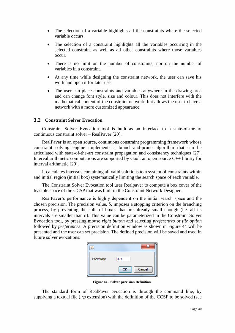
The Constraint Network Designer also allows the user to define a full set of options
on the network, so that the user may view it in a customized way. The options go from
font size and shape, colours and borders, as we can observe on Figure 42.
Figure 42 – Constraint network personalization
After the constraint network is defined, the corresponding CCSP can be solved. To
accomplish that, the user must press the solve option (Figure 43) which will trigger the
Constraint Solver Evocation described in next chapter.
Figure 43 – Solving a CCSP defined in a Constraint Network
3.1.4 Summary
To develop the Constraint Network Designer several options were discussed based,
not only on constraint programming concepts, but also on usability. The result is a set of
features that we can summarize as follows:
Once the user inserts a constraint (equation or inequality), the Constraint
Network Designer is able to identify which components of the constraint are
variables and represents them, automatically, as variables of the problem.
A variable must have an associated domain (an interval of reals). Once a
variable is identified, a default domain is automatically associated with it.
This domain is the interval [-100, 100].
Page 40
The selection of a variable highlights all the constraints where the selected
variable occurs.
The selection of a constraint highlights all the variables occurring in the
selected constraint as well as all other constraints where those variables
occur.
There is no limit on the number of constraints, nor on the number of
variables in a constraint.
At any time while designing the constraint network, the user can save his
work and open it for later use.
The user can place constraints and variables anywhere in the drawing area
and can change font style, size and colour. This does not interfere with the
mathematical content of the constraint network, but allows the user to have a
network with a more customized appearance.
3.2 Constraint Solver Evocation
Constraint Solver Evocation tool is built as an interface to a state-of-the-art
continuous constraint solver – RealPaver [20].
RealPaver is an open source, continuous constraint programming framework whose
constraint solving engine implements a branch-and-prune algorithm that can be
articulated with state-of-the-art constraint propagation and consistency techniques [27].
Interval arithmetic computations are supported by Gaol, an open source C++ library for
interval arithmetic [29].
It calculates intervals containing all valid solutions to a system of constraints within
and initial region (initial box) systematically limiting the search space of each variable.
The Constraint Solver Evocation tool uses Realpaver to compute a box cover of the
feasible space of the CCSP that was built in the Constraint Network Designer.
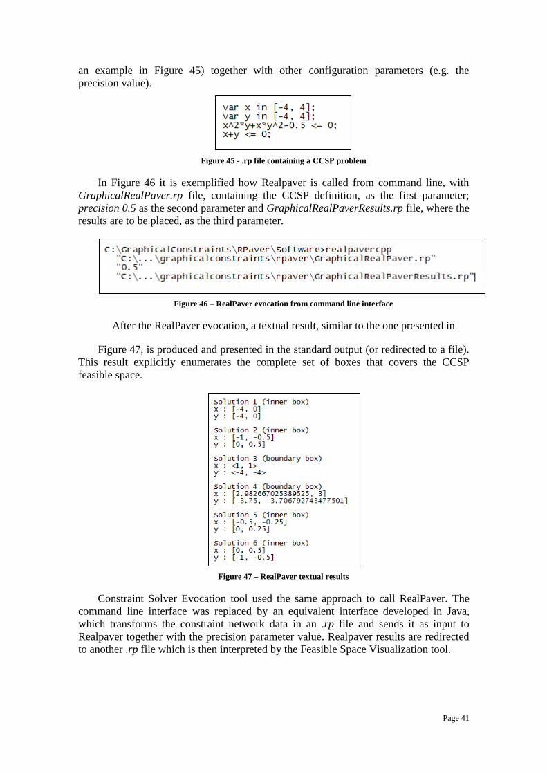
RealPaver’s performance is highly dependent on the initial search space and the
chosen precision. The precision value, , imposes a stopping criterion on the branching
process, by preventing the split of boxes that are already small enough (i.e. all its
intervals are smaller than ). This value can be parameterized in the Constraint Solver
Evocation tool, by pressing mouse right button and selecting preferences or file option
followed by preferences. A precision definition window as shown in Figure 44 will be
presented and the user can set precision. The defined precision will be saved and used in
future solver evocations.
Figure 44 - Solver precision Definition
The standard form of RealPaver evocation is through the command line, by
supplying a textual file (.rp extension) with the definition of the CCSP to be solved (see
Page 41
an example in Figure 45) together with other configuration parameters (e.g. the
precision value).
Figure 45 - .rp file containing a CCSP problem
In Figure 46 it is exemplified how Realpaver is called from command line, with
GraphicalRealPaver.rp file, containing the CCSP definition, as the first parameter;
precision 0.5 as the second parameter and GraphicalRealPaverResults.rp file, where the
results are to be placed, as the third parameter.
Figure 46 – RealPaver evocation from command line interface
After the RealPaver evocation, a textual result, similar to the one presented in
Figure 47, is produced and presented in the standard output (or redirected to a file).
This result explicitly enumerates the complete set of boxes that covers the CCSP
feasible space.
Figure 47 – RealPaver textual results
Constraint Solver Evocation tool used the same approach to call RealPaver. The
command line interface was replaced by an equivalent interface developed in Java,
which transforms the constraint network data in an .rp file and sends it as input to
Realpaver together with the precision parameter value. Realpaver results are redirected
to another .rp file which is then interpreted by the Feasible Space Visualization tool.

Page 42
3.3 Feasible Space Visualization
The Feasible Space Visualization tool always presents the feasible space cover in
textual format. Complementary, whenever the CCSP has two or three variables, this
information is also plotted as a 2D or 3D graphic, respectively. This cannot be achieved
for a higher number of variables due to the impossibility of its graphical representation.
Boxes are classified as inner or boundary boxes. Inner boxes (dark grey) are boxes
where all its points are solutions. Boundary boxes (light grey) are boxes where it is not
possible to prove that all points are solutions neither that all points are inconsistent.
Consider a CCSP with two variables, x and y, both ranging in the interval [-π, π]
and one inequality constraint 2 2 0.5x y xy . The left side of Figure 48 shows its
feasible space, while the right side shows its box cover with inner and boundary boxes.
When represented graphically, inner boxes are clearly inside the feasible space area,
while boundary boxes may have regions outside the feasible space. Note that some
boundary boxes are completely inside the feasible space (because the solver could not
prove that it only contains solutions) and others are completely outside the feasible
space (because the solver could not prove that they do not contain any solution).
Figure 48 - Inner boxes in dark grey and boundary boxes in light grey
The Feasible Space Visualization graphic is built by interpreting solver feasible
space solutions returned from the solver which are delivered in textual format.
Computation must be made to transform them into recognizable boxes to be plotted into
a graphic. Next those computations are described, both for 2D or 3D.
3.3.1 Computing 2D boxes
The textual representation of a 2D box returned by RealPaver has the following
format:
Solution 1 (inner box)
x : [-4, 0]
y : [-4, 0]

Page 43
This represents the boundaries of the box which is graphically shown in Figure 49
Figure 49 – Box x: [-4,0] and y:[-4.0] graphical representation
To represent the box graphically using jmathplot, the centre of the box is computed
and then the size of the box is calculated from the centre out to all sides.
Reading the first line x: [-4, 0] ,the variable x is identified and then the width of
the box is calculated.
Width = 0 – (-4)
Centre of the box on x axes = -4 + (0 – (-4)) / 2
Reading the second line y: [-4, 0] the rest of the box is obtained
Height = 0 – (-4)
Centre of the box on y axes = -4 + (0 – (-4)) / 2
3.3.2 Computing 3D boxes
The textual representation of a 3D box returned by RealPaver has the following
format:
Solution 1 (inner box)
x : [-0.8660254037844387, 0]
y : [-0.8660254037844387, 0]
z : [-0.8660254037844387, 0]
This represents the boundaries of the box which is graphically represented in Figure
50.

Page 44
Figure 50 - Box x : [-0.866, 0]; y : [-0.866, 0] ; z : [-0.866, 0] graphic
To represent the 3D box graphically using jmathplot, the centre of the box must be
computed and then the size of all sides of the box is calculated from the centre out to all
sides.
Reading the first line x: [-0.8660254037844387, 0], the variable x is identified
and then the width of the box is calculated.
Width = 0 – (-0.8660254037844387)
Centre of the box on x axis:
-0.8660254037844387 + (0 – (-0.8660254037844387)) / 2
A similar process is used to compute the height and depth of the box, as well as the
centre in the y and z axes.
3.3.3 Visualizing the feasible space box cover
After computing all the boxes graphical values, the feasible space box cover is
presented in a new window, both in textual format (on the left) and graphical (on the
right). Inner boxes are presented with a black border and boundary boxes are presented
with a grey border. Figure 51 presents the box cover of the CCSP with two variables, x
and y, both ranging in the interval [-4, 4] and one inequality constraint 2 2 0.5x y xy .
Page 45
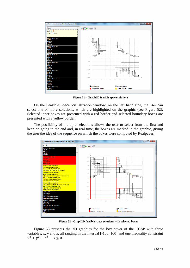
Figure 51 – Graph2D feasible space solutions
On the Feasible Space Visualization window, on the left hand side, the user can
select one or more solutions, which are highlighted on the graphic (see Figure 52).
Selected inner boxes are presented with a red border and selected boundary boxes are
presented with a yellow border.
The possibility of multiple selections allows the user to select from the first and
keep on going to the end and, in real time, the boxes are marked in the graphic, giving
the user the idea of the sequence on which the boxes were computed by Realpaver.
Figure 52 - Graph2D feasible space solutions with selected boxes
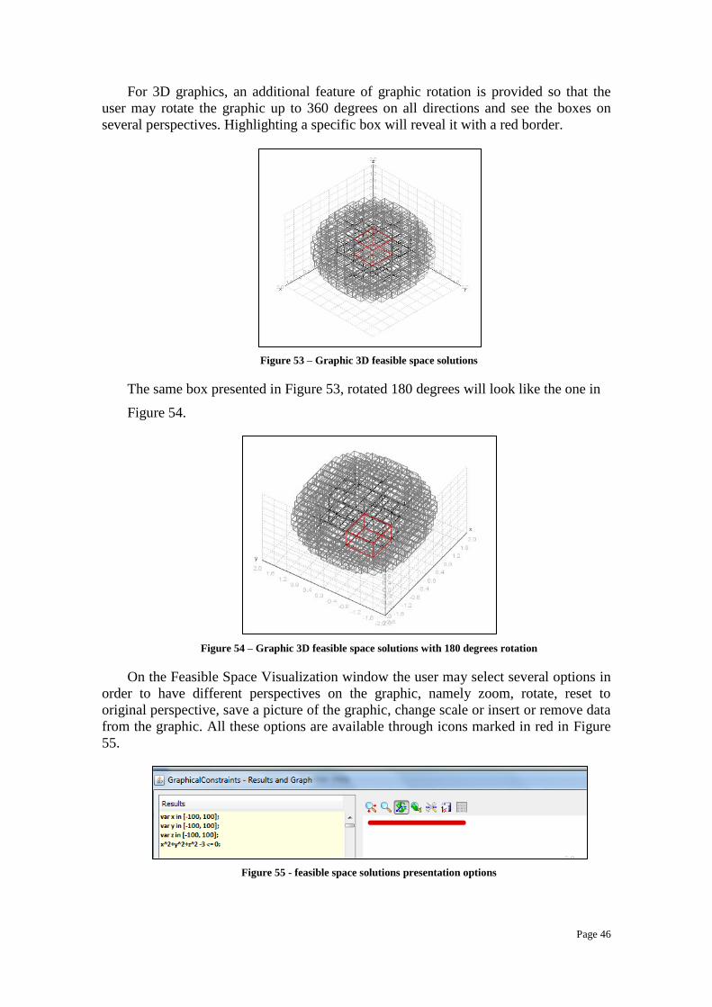
Figure 53 presents the 3D graphics for the box cover of the CCSP with three
variables, x, y and z, all ranging in the interval [-100, 100] and one inequality constraint
.
Page 46
For 3D graphics, an additional feature of graphic rotation is provided so that the
user may rotate the graphic up to 360 degrees on all directions and see the boxes on
several perspectives. Highlighting a specific box will reveal it with a red border.
Figure 53 – Graphic 3D feasible space solutions
The same box presented in Figure 53, rotated 180 degrees will look like the one in
Figure 54.
Figure 54 – Graphic 3D feasible space solutions with 180 degrees rotation
On the Feasible Space Visualization window the user may select several options in
order to have different perspectives on the graphic, namely zoom, rotate, reset to
original perspective, save a picture of the graphic, change scale or insert or remove data
from the graphic. All these options are available through icons marked in red in Figure
55.
Figure 55 - feasible space solutions presentation options

Page 47
By selecting the data icon (see Figure 56), the user is presented with a data table
(Figure 57) representing the data on the graphic. There are available data tables for
inner and boundary boxes, and for selected inner and boundary boxes. On the top of the
data table, the user may select or deselected the information he wants to get visible (see
Figure 57).
Figure 56 - Data icon
Figure 57 - Data table
An example of selecting and deselecting boxes can be done using the graphic on
Figure 58. On the figure, inner and boundary solutions are selected and plotted.
Figure 58 - Sphere with all the solutions plotted
Page 48
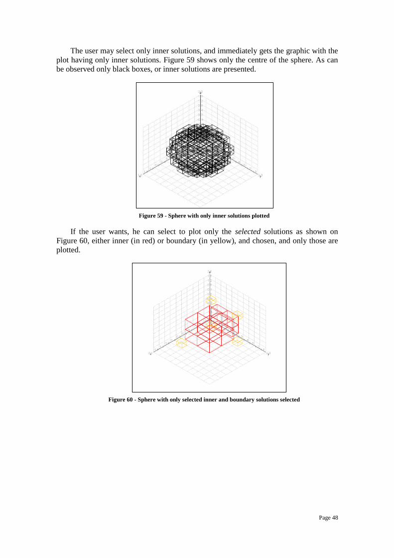
The user may select only inner solutions, and immediately gets the graphic with the
plot having only inner solutions. Figure 59 shows only the centre of the sphere. As can
be observed only black boxes, or inner solutions are presented.
Figure 59 - Sphere with only inner solutions plotted
If the user wants, he can select to plot only the selected solutions as shown on
Figure 60, either inner (in red) or boundary (in yellow), and chosen, and only those are
plotted.
Figure 60 - Sphere with only selected inner and boundary solutions selected
Page 49
3.4 Examples
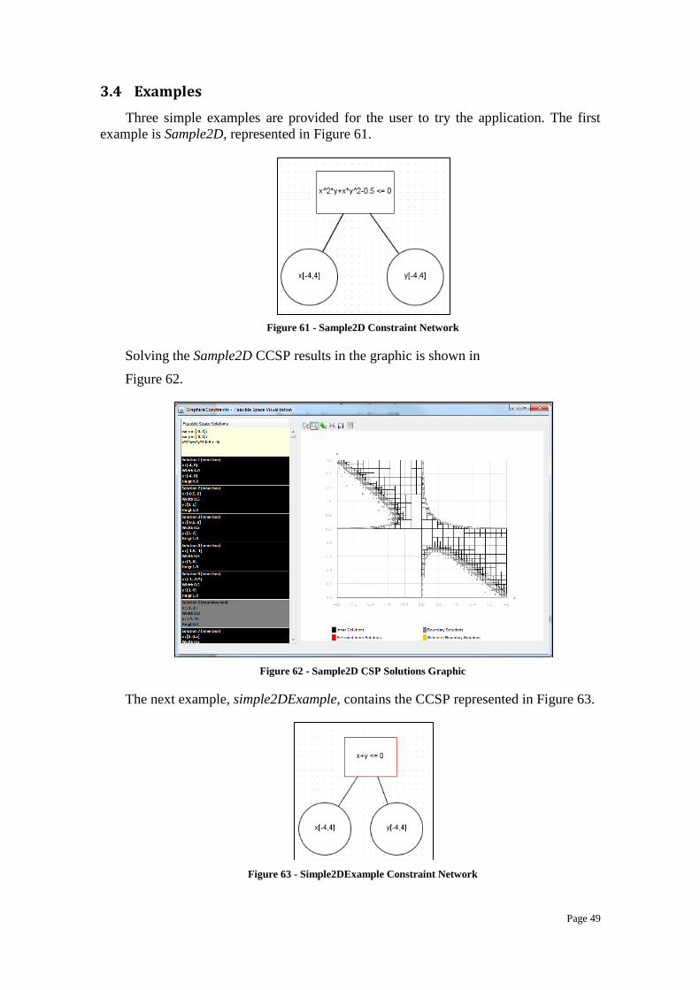
Three simple examples are provided for the user to try the application. The first
example is Sample2D, represented in Figure 61.
Figure 61 - Sample2D Constraint Network
Solving the Sample2D CCSP results in the graphic is shown in
Figure 62.
Figure 62 - Sample2D CSP Solutions Graphic
The next example, simple2DExample, contains the CCSP represented in Figure 63.
Figure 63 - Simple2DExample Constraint Network

Page 50
The feasible space cover of such CCSP is presented in Figure 64.
Figure 64 - Simple2DExample CSP Solutions Graphic
The last example, 3DSphere, in Figure 65 illustrates a CCSP with three variables,
representing a sphere, whose feasible space cover is presented in Figure 66.
Figure 65 – 3DSphere Constraint Network

Page 51
Figure 66 - 3DSphere CSP Solutions Graphic
3.5 Technical considerations
GraphicalConstraints was developed using Eclipse IDE, Version: Kepler Service
Release 2, which is suitable to develop both in Java and C++. Java was the
programming language used to develop the Constraint Network Designer and to plot the
feasible space solutions graphics.
C++ was the programming language used to compile RealPaver code which was
already developed. The compiled C++ executable was called from the Constraint Solver
Evocation tool.
The framework used to develop the Constraint Network Designer was mxGraph
and it was based on the GraphEditor framework provided on those libraries. The
mxGraph is a family of libraries, written in a variety of technologies, which provides
features aimed at applications that display interactive diagrams and graphs. It contains
all the commonly required functionality to draw, interact with and associate a context
with a diagram displayed in the technology of that particular mxGraph flavour.
The solver used is RealPaver and its evocation is made by the Constraint Solver
Evocation tool through a developed Java code that interprets constraint network,
transforms it to RealPaver syntax and calls RealPaver solver.
The Feasible Space Visualization component was developed using JMathTools,
which is a collection of independent packages designed to fit common
engineering/scientific computing needs and also classes of jmathplot to plot 2D and 3D
graphics. It was initially developed to provide easy to use Java API in Matlab to Java
porting task. In this project the used classes are jmathplot to plot 2D and 3D graphics.
3.5.1 GraphicalConstraints Installation and Execution
GraphicalConstraints needs no specific installation procedures. It is provided in a
folder containing all the needed resources and an executable JAR. Some examples,
already described, are also provided.
To execute GraphicalConstraints application, GraphicalConstraints folder must be
placed on the computer, and the application execution is made by executing
GraphicalConstraints. See folder contents in Figure 67.
Figure 67 - GraphicalConstraints installed folder
Page 52
4 Conclusions and future work
Continuous constraint satisfaction problems are complex and its representation in
terms of graphical user interfaces is of major importance so that it becomes appealing
and more intuitive to the user.
Specialized constraint solvers use constraints to search for consistent solutions. The
usability, success and popularity of the existing solvers are greatly enhanced by proper
and friendly user interfaces.
The project goal, as enunciated in the project proposal, was to develop a graphical
user interface on a constraint solver in continuous domains, which was successfully
accomplished. GraphicalConstraints - a graphical user interface that serves as a proof of
concept application to handle constraint satisfaction problems on continuous domains
was built and implements a graphical user interface on an existing solver.
GraphicalConstraints uses one of the most typical and common GUI’s, which
are those that allow users to click and drag objects with a mouse. It was used because
the kind of interaction needed was to draw the constraint network.
User interfaces are built to accomplish two main objectives: communicating
information from the system to the user, and communicating information from the user
to the system. GraphicalConstraints accomplishes those main goals: with a tool that
allows the design of a constraint network to input the constraints into the application;
and a tool to present the results in textual format and in 2D or 3D graphics.
A good user interface design makes a product easy to understand and use, which
results in greater user acceptance. With GraphicalConstraints, graphical representation
of a CCSP becomes easy. It allows a much better perception on the problem itself by
designing a constraint network and by graphically presenting the obtained feasible space
box cover, whenever it is possible.
Despite successfully achieving all the proposed goals, GraphicalConstraints is a
proof of concept that can be further enhanced.
The Constraint Solver Evocation tool could be extended to support a wider
parameterization of the RealPaver solver, allowing the use all its powerful features.
Moreover this tool could be complemented with interfaces to other state-of-the-art
solvers, providing the user a broader range of choices.
The Feasible Space Visualization tool could provide graphical representations of
problems with more than 3 variables. This would be achieved by projecting the feasible
space box cover in only 2 or 3 dimensions. The user would choose the variables on
which to project.
Other interesting feature would be to choose one or several boundary boxes in the
feasible space cover and be capable of call the solver over such boxes, with the same
constraints but a higher precision demand, to further prune the boxes.
Orthogonally, the GraphicalConstraints application could be extended to deal with
discrete Constraint Satisfaction Problems. This would have an impact in the three tools:
graphical representation of the problem; interface with a specialized solver and; the
results presentation.

Page 53
References
[1] Eugene C. Freuder. Constraints, April 1997
[2] Francesca Rossi, Peter Van Beek, Toby Walsh. Handbook of constraint
programming. Elsevier. p. 157. ISBN 978-0-444-52726-4, 2006
[3] Edward Tsang. Foundations of Constraint Satisfaction, Academic Press, London
and San Diego, 1993; Kim Marriott e Peter J. Stuckey. Programming with Constraints:
an Introduction, MIT Press, 1998.
[4] Lucas Augusto Carvalho. Mestrado em Ciência da Computação – 2011.1 DCOMP -
Universidade Federal de Sergipe, 2011.
[5] Stuart Jonathan Russell, Peter Norvig. Artificial Intelligence: A Modern
Approach. Prentice Hall. p. Chapter 6. ISBN 9780136042594, 2010.
[6] Jean-Louis Laurière. A Language and a Program for Stating and Solving
Combinatorial Problems. Artificial Intelligence. 10(1): 29-127, 1978
[7] "Constraint Satisfaction." Definitions.net.STANDS4..
<http://www.definitions.net/definition/CONSTRAINT SATISFACTION>, LLC, 2014,
Web. 18 Sep. 2014
[8] Stuart Russell and Peter Norvig. Artificial Intelligence: A Modern Approach
(Second Edition).
[9] Hicks, B. J., Medland, A. J., Mullineux, G., "The representation and handling of
constraints for the design, analysis and optimization of high speed machinery", Artificial
Intelligence for Engineering Design, Analysis and Manufacture (AIEDAM), 20 (2006)
313-328.
[10] P. Van Hentenryck and V. Saraswat. Constraint Programming: Strategic
Directions.
[11] J. Cruz. “Constraint Reasoning for Differential Models”. Pedro Barahona
(supervisor); PhD thesis. FCT/UNL, 2003.
[12] R. E. Moore. Interval analysis. Vol. 2. Prentice-Hall Englewood Cliffs, 1966.
[13] Laurent Granvilliers, Solving Nonlinear Constraints by Interval Computations,
Edition 0.4, for RealPaver Version 0.4 August 2004
Page 54
[14] Boi Faltings. Arc Consistency for Continuous Variables. Artificial
Intelligence, 65(2):363-376, 1994.
[15] Constraint Branching Techniques, Alastair McNaughton Department of
Mathematics University of Auckland; David Ryan Department of Engineering Science
University of Auckland
[16] Principles of Constraint Programming Krzysztof R. Apt CWI, Amsterdam,
The Netherlands
[17], M. Gutierrez Miranda Universidad Autonoma Metropolitana (Mexico), The
importance of graphic users interface, analysis of graphical user interface design in the
context of human-computer interaction
[18] Dillon, A, User Interface Design. MacMillan Encyclopedia of Cognitive
Science, Vol. 4, London: MacMillan, 453-458, 2003
[19] Xuan-Ha VU (2005) Rigorous solution techniques for numerical constraint
satisfaction problems, Thesis Number 3155, 2005
[20] Laurent Granvilliers - RealPaver User’s Manual - Solving Nonlinear
Constraints by Interval Computations Edition 0.4, for RealPaver Version 0.4 August
2004
[21] Myers, Brad A, A Brief History of Human-Computer Interaction Technology.
In Interactions, 5 (2) pp. 44-54, 1998
[22] Alefeld and Herzberger, Introduction to Interval Computation, First edition,
Academic Press, 1983
[23] A. Neumaier, Interval Methods for Systems of Equations, Cambridge
University Press, 1990
[24] L. Jaulin, M. Kieffer, O. Didrit and E. Walter, Applied Interval Analysis,
Springer, 2001
[25] Eldon Hansen (Editor), G. William Walster, Global Optimization Using
Interval Analysis, Revised And Expanded (Pure and Applied Mathematics (M.
Dekker)), 2003

Page 55
[26] Hickey, M.P., Schubert, G. and Walterscheid, R.L, Acoustic wave heating of
the thermosphere. Journal of Geophysical Research 106: doi: 10.1029/2001JA000036.
issn: 0148-0227, 2001
[27] Elsa Cristina Bento Carvalho, Probabilistic Constraint Reasoning, Faculdade
de Ciencias e Tenologia de Lisboa, Universidade Nova de Lisboa 2012
[28] Shneiderman, B, Designing the user interface: Strategies for effective human-
computer interaction. Reading, MA: Addison-Wesley, 1987
[29] Gaol, Not Just Another Interval Library. www.sourceforge.net/projects/gaol.
18, 107
[30] H. Collavizza, F. Delobel, and M. Rueher. A note on partial consistencies over
continuous domains. Lecture Notes in Computer Science, 1520:147–161, 1998.
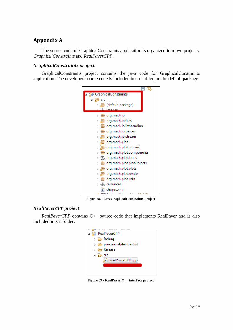
Page 56
Appendix A
The source code of GraphicalConstraints application is organized into two projects:
GraphicalConstraints and RealPaverCPP.
GraphicalConstraints project
GraphicalConstraints project contains the java code for GraphicalConstraints
application. The developed source code is included in src folder, on the default package:
Figure 68 - JavaGraphicalConstraints project
RealPaverCPP project
RealPaverCPP contains C++ source code that implements RealPaver and is also
included in src folder:
Figure 69 - RealPaver C++ interface project

Page 57
GraphicalConstraints folder
GraphicalConstraints folder contains GraphicalConstraints executable jar,
RealPaver folder which contains all the resource files needed to communicate with
RealPaver and the three samples provided.
Figure 70 - GraphicalConstraints folder
RPaver folder
RPaver folder contains a Software folder with RealPaver executables and three files
used to communicate with RealPaver. GraphicalRealPaver is used as input to
RealPaver and contains the problem to be solved. GraphicalRealPaverPreferences
stores GraphicalConstraints preferences to be used by RealPaver. In this version, the
feasible space solutions precision is the only preference stored.
GraphicalRealPaverResults is used by RealPaver to return feasible space solutions.
Figure 71 - Rpaver folder
Figure 72 - Software folder within RPaver
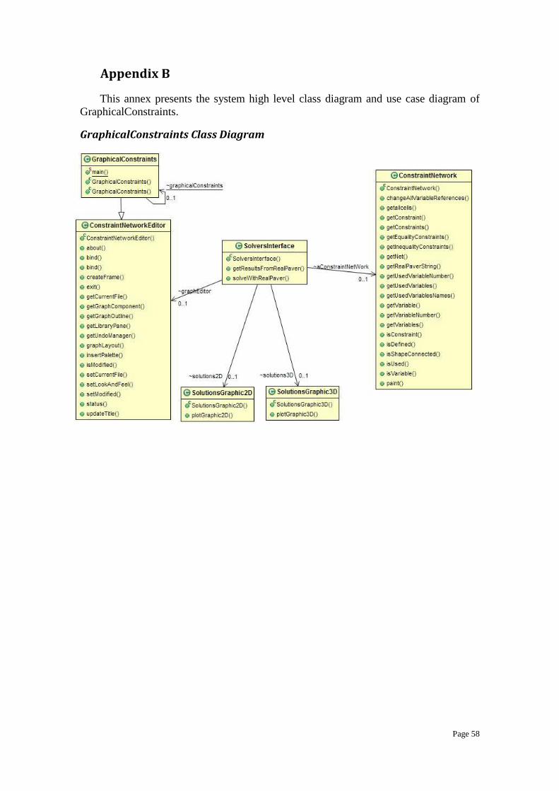
Page 58
Appendix B
This annex presents the system high level class diagram and use case diagram of
GraphicalConstraints.
GraphicalConstraints Class Diagram

Page 59
Use Case Diagram