This content has been downloaded from IOPscience. Please scroll down to see the full text.

Download details:

IP Address: 144.217.70.220

This content was downloaded on 31/05/2018 at 07:37

Please note that terms and conditions apply.

You may also be interested in:

Radiative Properties of Semiconductors: Graphene

N M Ravindra, S R Marthi and A Bañobre

Electron transport in graphene

S V Morozov, K S Novoselov and A K Geim

Optimization of Immobilization of Nanodiamonds on Graphene

A Pille, S Lange, K Utt et al.

Doping graphene with a monovacancy: bonding and magnetism

M Yu Arsent'ev, A V Prikhodko, A V Shmigel et al.

About a permeability of graphene pores

Mikhail A Bubenchikov, Alexander I Potekaev, Alexey M Bubenchikov et al.

Bubbles in graphene - a computational study

Mikkel Settnes, Stephen R Power, Jun Lin et al.

Graphene quantum dot with a hydrogenic impurity

Neslihan Gökçek and Bekir Stk Kandemir

Graphene quantum dot with a hydrogenic impurity

Neslihan Gökçek and Bekir Stk Kandemir

Korea targets graphene research

Matin Durrani

IOP Concise Physics

Graphene Optics: Electromagnetic Solution of

Canonical Problems

Ricardo A Depine

Chapter 1

Electromagnetics of graphene

This chapter summarizes the aspects of macroscopic electromagnetism that form thebasis of this book. The emphasis is placed on topics that are essential to understandthe approach used to model the electromagnetic response of graphene, such as thedistinction between the bound charges and currents associated with atoms ormolecules and the free charges and currents associated with external sources; howthe bound sources are described in terms of polarization and magnetizationdensities; the formulation of constitutive relations in the frequency domain; theKubo model for graphene surface conductivity, the form of the fields in piecewisehomogeneous materials; and the boundary conditions in the presence of a graphenelayer.

1.1 Macroscopic electrodynamicsThe electromagnetic field can be described as the combination of electric andmagnetic fields produced by charges and currents, i.e. electrically charged movingobjects. Due to the microscopic nature of matter, all matter is an ensemble ofdiscrete charges dispersed in free space or vacuum, and bound charges and currentsare induced in a material in the presence of electromagnetic fields. Macroscopicelectrodynamics can be formulated starting from the fundamental laws of electro-magnetism in vacuum. However, this formulation involves the description of thevery complicated and granular microscopic sources, and the drastic variations inspace they produce on the microscopic fields. In order to avoid such problems,macroscopic electrodynamics is instead formulated in terms of averaged fields andsources, which describe the behavior of fields and sources measured with aninstrument of macroscopic dimensions. All averages are performed over asufficiently large scale, much larger than individual atomic sizes so as not to see

doi:10.1088/978-1-6817-4309-7ch1 1-1 ª Morgan & Claypool Publishers 2016

the granularity of the atomic sources, but also sufficiently small compared to thedistances accessible to experimentation [1].

We start with macroscopic Maxwell’s equations in SI units:

∇ × = −∂∂

E rB

rtt

t( , ) ( , ) (1.1)

∇ × = ∂∂

+H rD

r J rtt

t t( , ) ( , ) ( , ) (1.2)

ρ∇ · =D r rt t( , ) ( , ) (1.3)

∇ · =B r t( , ) 0, (1.4)

where =r x y z( , , ), t denotes the time, E denotes the electric field, D denotes theelectric displacement, B and H denote the magnetic fields, and ρ and J denote thefree charge and current volume densities, respectively, that is, the free sources notassociated with any particular atom or molecule. Since magnetic terminology can beconfusing—magnetic induction and magnetic field are used in the literature todescribe either B or H without distinction—conventional names for B and H areavoided in this book. Taking into account the fact that E and B appear in theLorentz force acting on a point charge rq t( , ) travelling at velocity v r t( , ),

= + ×F r E r v r B rq t t t t( , )[ ( , ) ( , ) ( , )], (1.5)Lor

the fundamental electromagnetic quantity, E and B, may be therefore calledprimitive fields, while D and H are macroscopic fields induced by the presence ofmaterial interactions and may be appropriately termed induction fields.

Macroscopically averaged bound charges and currents are described in terms ofthe polarization density P r t( , ), representing the electric dipole moment per unitvolume, and the magnetization density M r t( , ), representing the magnetic dipolemoment per unit volume. The macroscopic bound charge density ρ r t( , )b and boundcurrent density J r t( , )b are

ρ = −∇ · P (1.6)b

= ∇ × + ∂∂

J MPt

. (1.7)b

1.2 Constitutive relationsThe use of D and H has the advantage that only the free sources, not the boundones, appear explicitly in equations (1.2) and (1.3), that is, in Maxwell equationsinvolving the sources. However, the information about the bound sources given by

Graphene Optics: Electromagnetic Solution of Canonical Problems

1-2

equations (1.6) and (1.7) is of course not irrelevant. In fact, P and M appear in thedefinition of D and H :

ε= +D E P (1.8)0

μ= −−H B M , (1.9)01

where ε0 and μ0 are, respectively, the electric permittivity and magnetic permeabilityof vacuum, ε μ = −c0 0

1, and c is the velocity of light in vacuum. The behavior of Pand M under the influence of the fields results from the microscopic structure of thematerial. The equations describing this behavior are known as constitutive relations.In some cases the determination of P and M in terms of E and B can be derivedfrom first principles, using the tools of condensed matter physics, whereas in othercases this determination is based directly upon measurements. Constitutive relationscan be symbolically expressed in the following form [1]:

=D D E B[ , ] (1.10)

=H H E B[ , ]. (1.11)

For conducting media, i.e. media that generate an electric current in the presence ofan electric field, it is sometimes convenient to split J , the current volume density notassociated with any particular atom or molecule, into an external current densityJ (ext) that is associated with external sources, and an induced current density J (cond)

that is associated with the conduction carriers:

= +J J J . (1.12)(cond) (ext)

In this case, a generalized Ohm’s law

=J J E B[ , ] (1.13)(cond) (cond)

must also be given. Square brackets were used to denote that the connectionsbetween the induced and the primary quantities are not necessarily simple. Forexample, these connections may include the dependence of D and H (or equiv-alently, of P and M ) on E and B at other locations and times. The study ofconstitutive relations provides a basis for the classification of media using certaincriteria, such as distinctions on the basis of linearity versus nonlinearity, isotropyversus anisotropy, homogeneity versus nonhomogeneity, spatial and/or temporaldispersion, and so on [2]. Some of the most common materials have a linear responseto applied fields over a wide range of field values. The constitutive relations for alinearmedium are generally nonlocal with respect to both space and time and can bewritten as [2, 3]:

∫ ε

ξ

= ′ ′ ˇ ′ ′ · − ′ − ′

+ ˇ ′ ′ · − ′ − ′

⎡⎣⎤⎦

D r r r E r r

r B r r

t t t t t

t t t

( , ) d d ( , ) ( , )

( , ) ( , )(1.14)

3EB

EB

Graphene Optics: Electromagnetic Solution of Canonical Problems

1-3

∫ ζ

ν

= ′ ′ ˇ ′ ′ · − ′ − ′

+ ˇ ′ ′ · − ′ − ′

⎡⎣⎢

⎤⎦⎥

H r r r E r r

r B r r

t t t t t

t t t

( , ) d d ( , ) ( , )

( , ) ( , ) ,(1.15)

3EB

EB

where ε̌ r t( , )EB , ξ̌ r t( , )EB , ζ̌ r t( , )EB and ν̌ r t( , )EB are second order tensors. Temporalnonlocality refers to the fact that the induction fields D and H (and therefore theinduced sources) at time t depend on the values of E and B at all times ′t previousto t. Similarly, spatial nonlocality refers to the fact that D and H at location rdepend on the values of E and B at neighboring locations ′r . While temporalnonlocality, a consequence of causality [4], is a widely encountered phenomenonthat must be accurately taken into account, spatial nonlocality can play a significantrole when some characteristic length scale in the medium is short with respect to thewavelength, but can usually be neglected for visible light or electromagneticradiation of longer wavelengths [5]. Restricting ourselves to linear, spatially localmaterials, the constitutive relations take the form:

∫ ε ξ= ′ ˇ ′ · − ′ + ˇ ′ · − ′⎡⎣ ⎤⎦D r r E r r B rt t t t t t t t( , ) d ( , ) ( , ) ( , ) ( , ) (1.16)EB EB

∫ ζ ν= ′ ˇ ′ · − ′ + ˇ ′ · − ′⎡⎣ ⎤⎦H r r E r r B rt t t t t t t t( , ) d ( , ) ( , ) ( , ) ( , ) . (1.17)EB EB

1.3 From the time domain to the frequency domainIn equations (1.14) and (1.15), spatial and temporal nonlocality are displayed asconvolutions between constitutive tensors and fields. Thanks to the convolutiontheorem [6], constitutive equations are more conveniently handled in the domainof the angular frequency ω and the wavevector k, the Fourier conjugate variables forthe time coordinate t and the space coordinate r, respectively. For spatially localmaterials, only the angular frequency ω is relevant. After taking the temporalFourier transforms of equations (1.16) and (1.17), the following frequency-domainconstitutive relations can be obtained

ε ξω ω= · + ·ω ω ωD r r E r r B r( ) ( , ) ( ) ( , ) ( ) (1.18)EB EB

ζ μω ω= · + ·ω ω ωH r r E r r B r( ) ( , ) ( ) ( , ) ( ), (1.19)EB EB

with ωE r( ), ωB r( ), ωD r( ) and ωH r( ) being the temporal Fourier transforms of theelectromagnetic fields, and ε ωr( , )EB , μ ωr( , )EB , ξ ωr( , )EB and ζ ωr( , )EB beingthe temporal Fourier transforms of the constitutive tensors. Here we follow theconvention that the inverse temporal Fourier transform incorporates a −i factor inthe exponential term, so a time-dependent quantity rF t( , ) in terms of its Fouriertransform is obtained as

∫ ω= ωω

−∞

∞−r rF t F( , ) ( )e d . (1.20)i t

Graphene Optics: Electromagnetic Solution of Canonical Problems

1-4

The form of equations (1.18) and (1.19), known as the Boys–Post representation [3],denotes the natural roles of E and B as the fundamental or primitive fields and Dand H as the derived or induction fields. However, in common practice the Tellegenrepresentation [3]

ε ξω ω= · + ·ω ω ωD r r E r r H r( ) ( , ) ( ) ( , ) ( ) (1.21)EH EH

ζ μω ω= · + ·ω ω ωB r r E r r H r( ) ( , ) ( ) ( , ) ( ) (1.22)EH EH

is usually preferred, with ε ωr( , )EH , μ ωr( , )EH , ξ ωr( , )EH and ζ ωr( , )EH being the

temporal Fourier transforms of the constitutive tensors ε̌ r t( , )EH , ξ̌ r t( , )EH , ζ̌ r t( , )EHand ν̌ r t( , )EH .

1.4 Isotropic mediaFor most materials P and J (cond) are parallel to E and M is parallel to B. Thesematerials are known as isotropic dielectric–magnetic materials and their constitutiverelations have the simple form

ε ε ω=ω ωD r r E r( ) ( , ) ( ) (1.23)0

μ μ ω=ω ωB r r H r( ) ( , ) ( ) (1.24)0

σ ω=ω ωJ r r E r( ) ( , ) ( ), (1.25)(cond) 3D

where σ3D is the electric conductivity, ε is the scalar electric permittivity and μ is thescalar magnetic permeability. For passive media, and as a consequence of the signconvention used for the exponential term in equation (1.20), the complex valuedconstitutive scalars ε and μ lie on the upper half of the complex plane, whereas σ3D

lies on the right half of the complex plane.The classical vacuum is both isotropic and homogeneous. It is the reference

medium of classical electromagnetism and its time-domain constitutive relationsemerge from the definition of D and H when all the material interactions areremoved. In this case, =P 0, =M 0 and =J 0(cond) , and from equations (1.8) and(1.9) we obtain

ε=D r E rt t( , ) ( , ) (1.26)0

μ=B r H rt t( , ) ( , ). (1.27)0

As ε0 and μ0 are true constants, the corresponding frequency-domain constitutiverelations have the same form as equations (1.23) and (1.24), but with ε ω =r( , ) 1,μ ω =r( , ) 1 and σ ω =r( , ) 03D .

1.5 Conductivity and permittivity formulationsWe observe that the right-hand side in Ampère’s law equation (1.2) has contribu-tions associated with current densities of different natures. As shown from the

Graphene Optics: Electromagnetic Solution of Canonical Problems

1-5

definition of D given by equation (1.8), the first term ∂ ∂D t/ gives one contributionthat is proportional to the rate of change of the electric field E , which is present evenin vacuum, and another contribution that is proportional to the rate of change of theelectric polarization P, which represents polarization currents associated withoscillating bound charges and is given by the second term in equation (1.7).According to equation (1.12), the second term on the right-hand side in Ampère’slaw equation (1.2), representing the free current density, can also be separated intotwo other contributions, one from the external sources and the other from inducedcarriers.

To work with the easy form of the constitutive relations, it is now convenient toconsider the frequency-domain version of equation (1.2). Doing so and using theconstitutive equation (1.23) for ωD , the separation equation (1.12), and theconstitutive equation (1.25) for ωJ (cond), we obtain

ωε ε ω σ ωωε

∇ × = − + +ω ω ω⎡⎣⎢

⎤⎦⎥H r r

rE r J ri

i( ) ( , )

( , )( ) ( ). (1.28)0

3D

0

(ext)

The right-hand side of this equation shows that all the contributions to currentdensity that are not associated with an external source are represented, for linearmedia, by a term that is proportional to the temporal Fourier transform of theelectric field ωE r( ). In addition, it shows that the contribution from the displacementcurrents coming from ∂ ∂D t/ and that from the conduction carriers coming fromOhm’s law are both treated on the same footing through the factor in squarebrackets in equation (1.28)

ε ω ε ω σ ωωε

= +⎡⎣⎢

⎤⎦⎥r r

ri( , ) ( , )

( , ), (1.29)(eff)

3D

0

which represents an effective dielectric constant to which all the constitutiveproperties of the medium can be attributed. We observe that this effective dielectricconstant does not distinguish between conduction currents and polarizationcurrents, which reflects the physical fact that no fundamental difference betweenthe conductors and dielectrics exists for oscillatory fields. This is the case because, asthe resulting oscillatory motion of all charges is spatially localized, the separationof the current into a polarization part and a free part is not really possible and theonly combination that can ever matter is the sum [7].

Both the constitutive parameter associated with bound polarization charges andthe effective dielectric constant represented by equation (1.29) are usually denotedby the same symbol, ε ωr( , ). This ambiguous notation should not lead us to forgetthat, when using an effective dielectric constant or a dielectric constant and aconductivity, we are using two different formulations of electromagnetism whichdiffer regarding how the conduction carriers are treated. The fundamental or

Graphene Optics: Electromagnetic Solution of Canonical Problems

1-6

primitive fields ωE and ωB in these two formulations are the same, but the derived orauxiliary fields ωD and ωH are different [7, 8].

1.6 Constitutive relations of grapheneGraphene is a single layer of a graphite crystal. It consists of a single atomic layer ofpure covalently bonded carbon atoms arranged in a two-dimensional (2D) hexag-onal lattice structure. Each carbon atom has six electrons surrounding its nucleus,two in the inner shell and four in the outer electron shell. Of these four electrons,three are bound with the nearest-neighbor atom electrons and create the strongchemical bonds that make graphene one of the strongest materials known to man,whereas the other electron in the outer electron shell of each carbon atom isdelocalized on the whole graphene layer [9].

The energy band structure of the delocalized electron determines graphene’sconductivity. While in non-conducting or semiconducting materials the full valenceband and the empty conduction band are separated by an energy gap, there is no gapbetween the conduction and valence bands in pure graphene. Thus, pure graphenecan be regarded as a zero-gap semiconductor. Similarly, while in metals the valenceband is partially filled, in pure graphene the Fermi level lies at the point where theconduction and valence bands meet (the Dirac point). Thus, pure graphenecan be regarded as a metal with an empty valence band. This duality between thezero-gap-semiconductor picture and the metal-with-an-empty-valence-band picturemakes graphene particularly interesting for applications in many photonic devicesthat require conducting but transparent thin films.

The duality between semiconductor and metallic behavior can be controlled bytuning the position of the Fermi level from the Dirac point, either by chemicaladditions, or, more easily, by using the electric field effect [10]. For example, when aconstant voltage (the gate voltage) is applied between graphene and a metallic layer,separated by a very thin insulator, the resulting electrical field will modify thequantity of conduction carriers and thus graphene’s electrical conductivity. For agiven polarity of the voltage, that is, for a given direction of the dc electric field, theconduction band fills up, which means that electrons are added to the system. Forthe other polarity, the number of electrons in the valence band is reduced, whichmeans that holes are added to the system.

Graphene constitutive equations can be well described using the Schrödinger-equation-based methods of condensed matter physics. In 1947, more than half acentury before its deliberate fabrication, the electronic structure of graphene wasexplored and its unusual properties were demonstrated by P R Wallace [11]. Themotivation of his work was to use a single-layer formalism as a starting point todetermine the electronic properties of bulk graphite. Using a band theory of solidswith a tight-binding approximation, Wallace was able to explain many of thephysical properties of graphite.

A relevant result from Wallace’s pioneering study is the fact that in graphiteelectronic currents only take place in layers, in other words, along a graphene layer.

Graphene Optics: Electromagnetic Solution of Canonical Problems

1-7

Therefore, a logical choice for incorporating a graphene layer into Maxwell’sequations is to model it using concepts such as conductivity surface, sheet resistanceor surface impedance. These concepts are widely applied in microwave electronicsand antenna theory when thin films are considered as 2D entities [12, 13], or whenthe current J (cond) in conducting boundaries is confined to such a small thickness justbelow the surface of the conductor that is equivalent to an effective surface currentK ([1], pp 354–6). For a linear and isotropic conductivity surface, the coefficient ofproportionality σ ω( ) linking the surface current and the tangential component of theelectric field along the plane of the sheet is called surface conductivity. In this case,the 2D analogue of the constitutive equation (1.25) is written as

σ ω=ω ωK E( ) . (1.30)

The inverse of σ ω( ), the coefficient of proportionality linking the tangentialcomponent of the electric field and the surface current along the plane of the sheet,is usually called surface impedance ([1], pp 354–6, [14]). In this book we deal withsituations in which graphene exhibits a local, linear and isotropic response.

As an alternative to the infinitesimally thin current sheet model, a homogeneousfilm of finite thickness δ can also be used to simulate a graphene layer [15], with thecurrent ωK evenly spread through the thickness of the film. The volume currentdensity ωJ (cond) is then δ=ω ωJ K /(cond) , and from equation (1.25) it follows that

σ ω σ ω δ=( ) ( ) . (1.31)3D

Therefore, according to equation (1.29), the effective dielectric constant of thishomogeneous film is

ε ω ε σ ωωε δ

= +⎡⎣⎢

⎤⎦⎥

i( ) 1

( ). (1.32)0

0

1.7 Ohmic lossesRecalling the constitutive equation (1.30) and taking into account the fact that thetime-averaged rate of work done per unit time per unit volume by the electro-magnetic fields on a current volume distribution is ·ω ω

*J ERe { }/2 [1], it follows thatthe time-averaged rate of work done per unit time per unit surface by the electro-magnetic fields on the graphene charge carriers is

σ σ= = =ω ω ω ω*{ }K E E EPa

dd

12

Re12

Re{ }Re

2, (1.33)2 2

where the asterisk is used to denote the complex conjugate of a complex number andwe have used the notation P ad /d to recall that this quantity is the time-averagedpower transferred from the electromagnetic field to the graphene carriers per unitarea.

Graphene Optics: Electromagnetic Solution of Canonical Problems

1-8

1.8 Kubo model for the surface conductivityBoth the conductivity surface and the thin film model for a graphene sheet requireknowledge of the frequency-dependent surface conductivity σ, a quantity which canbe obtained from either a microscopic model [13, 16–25] or from measurements[26–28]. Here we use the following high-frequency expression derived from the Kubomodel [13, 22, 25]

∫

∫

σ ωω γπ

ϵω γ

ϵϵ

ϵ

ϵ ϵω γ ϵ

ϵ

=+ℏ +

−− −

+ − ℏ

−∞

+∞

+∞

⎡⎣⎢

⎤⎦⎥

e i

i i

f

f f

i

( )( )

( )

d ( )

dd

( ) ( )

( ) 4( )d ,

(1.34)

c

c

c

2

2 20

0

0 02 2

where −e is the electron charge, πℏ = h/2 is the reduced Planck constant, γc is aphenomenological carrier scattering rate that is assumed to be independent of theenergy ϵ, ϵ ϵ μ= − + −f k T( ) {exp[( )/ ] 1}c0

1B is the Fermi function, μc is the chemical

potential (controlled with the help of a gate voltage), kB is Boltzmann’s constant andT is the ambient temperature. The first term in equation (1.34) corresponds tointraband electron–photon scattering processes, whereas the second term corre-sponds to the direct interband electron transitions.

For undoped (no chemical additions) and ungated (zero gate voltage) graphene at=T 0 K, the charge carrier density n0 is very low, but it can be tuned by chemical

additions (doping) or with the help of a constant electric field (electric field effect,gate voltage). The chemical potential is determined through the condition

∫πϵ ϵ ϵ μ ϵ=

ℏ− +

∞ ⎡⎣ ⎤⎦nv

f f2

( ) ( 2 ) d , (1.35)c0 2F2

00 0

where ≈v 9.5F · 105 m s−1 is the Fermi velocity.

1.8.1 Intraband conductivity

The intraband term in equation (1.34) results in

σ ωπ ω γ

μ=ℏ +

⎡⎣ ⎤⎦( )ie k Ti

k T( )2

( )ln 2 cosh 2 , (1.36)

cc

intra2

B2 B

which coincides with the conductivity given by the classical Drude–Boltzmannapproximation [25]. The real part of this term (zero for γ = 0c ) contributes to energyabsorption or dissipation due to the intraband electrons. Except for a factor whichaccounts for the interlayer separation between graphene planes, equation (1.36) forμ = 0c coincides with the expression derived by Wallace for graphite [11] andcorresponds to the intraband conductivity of a single-wall carbon nanotube in thelimit of infinite radius [12]. If μ ≫ k Tc B , the carriers are degenerate and the materialacts like a metal. In this case [30], μ π≈ ℏn v/c0

2 2F2, the chemical potential can be

Graphene Optics: Electromagnetic Solution of Canonical Problems

1-9

expressed as μ π≈ ≈ ℏE v nc F2

F2

0 , where EF is the Fermi energy, and the intrabandterm can be approximated by the Drude form

σ ωμ

π ω γ=

∣ ∣ℏ +

ie

i( )

( ). (1.37)c

c

intra2

2

It can be seen that σ ⩾Re 0intra and σ >Im 0intra , where Re and Im stand for thereal and imaginary parts of a complex quantity. Therefore, σ intra corresponds to asurface impedance Z (the inverse of the surface conductivity), with <ZIm 0, that is,an inductive surface impedance. As is well known for metallic boundaries [29], thesign of the imaginary part of the surface impedance plays an important role in thetype of surface waves that can be guided by the boundary. Therefore, it is notsurprising to find that, depending on the sign of the imaginary part of its complexsurface conductivity, a graphene sheet can support TE or TM surface plasmons,a type of surface waves that represent the collective oscillations of surface charges[23, 30, 31], which will be discussed later.

1.8.2 Interband conductivity

The interband contribution to the conductivity also has real and imaginary parts.For low temperatures, μ∣ ∣ ≫ k Tc B , it can be written as [20, 25]

σ ωπ

ω γ μ

πω γ μ

ω γ μ

=ℏ

+ℏ + −

−ℏ + +

ℏ + − +

⎪⎪

⎪⎪

⎧⎨⎩

⎡⎣ ⎤⎦⎡⎣ ⎤⎦

⎫⎬⎭

e i

k T

i i

i k T

( )4

12

1arctan

( ) 2

2

2ln

( ) 2

( ) 2 (2 ),

(1.38)

c c

c c

c c

inter2

B

2

2B

2

which can be closely approximated by [13, 20, 22]

σ ω θ ω μπ

ω γ μω γ μ

=ℏ

ℏ − +ℏ + − ∣ ∣ℏ + + ∣ ∣

⎡⎣⎢⎢

⎤⎦⎥⎥

e i i

i( )

4( 2 ) ln

( ) 2

( ) 2, (1.39)c c

c c

inter2

where θ ω μℏ − ∣ ∣( 2 ) is a step function. This expression shows that for γ = 0c ,σ =Re 0inter and σ <Im 0inter , that is, the interband contribution to the conductivity

is purely imaginary and negative. Therefore, under these conditions, σ inter corre-sponds to a surface impedance Z with >ZIm 0, i.e. a capacitive surface impedance.

Other approximations for the interband contribution in different regimes can befound in the literature [25]. In the most general case, calculating the interband termrequires that the integration indicated in the second term in equation (1.34) isperformed. To avoid the singular integral, it is convenient to use the followingequivalent form [25]

Graphene Optics: Electromagnetic Solution of Canonical Problems

1-10

∫σ ω ωω γ

πϵ ω

ω γ ϵϵ=

ℏ−

+ℏ

−+ − ℏ

+∞⎡⎣⎢

⎤⎦⎥

eG

i

iG G

i( )

4( 2)

4( ) ( ) ( 2)( ) 4( )

d , (1.40)c

c

inter2

0 2 2

where ϵ ϵ ϵ= − −G f f( ) ( ) ( )0 0 . Taking into account the fact that in the high-frequencylimit, ω μℏ ≫ k T( , )cB , ϵ ϵ→G k T( ) tanh( /2 )B , this expression shows that, in thislimit, σ → 0inter , and the total conductivity becomes mostly real and tends to theuniversal value ℏe /42 [32], independent of any material parameters.

It is useful to write the conductivity in units of ℏe /2 . In dimensionless form,

σ σ α πε σ=ℏ

˜ = ˜e

c(4 ) , (1.41)2

0

with

απε

μπ

=ℏ

=ℏ

ec

e c14 4

(1.42)0

20

2

being the fine-structure constant. As a dimensionless quantity, α has the samenumerical value, α ≈− 137.0361 , in all systems of units. In the Gaussian unit system,where the elementary charge is measured in statcoulombs [1], instead of in coulombsas in the SI system, α takes the form ℏe c/( )2 and σ α σ= ̃c(Gaussian) .

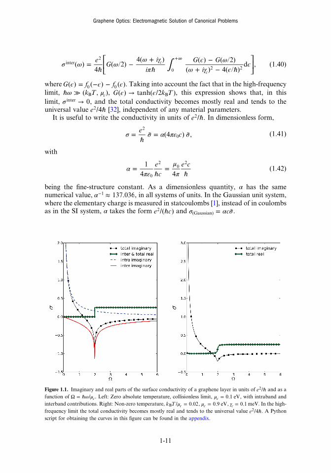
Figure 1.1. Imaginary and real parts of the surface conductivity of a graphene layer in units of ℏe /2 and as afunction of ω μΩ = ℏ / c. Left: Zero absolute temperature, collisionless limit, μ = 0.1 eVc , with intraband andinterband contributions. Right: Non-zero temperature, μ =k T / 0.02cB , μ = 0.9 eVc , γ = 0.1c meV. In the high-frequency limit the total conductivity becomes mostly real and tends to the universal value ℏe /42 . A Pythonscript for obtaining the curves in this figure can be found in the appendix.

Graphene Optics: Electromagnetic Solution of Canonical Problems

1-11

1.8.3 Material dispersion

In agreement with the experimental data [26–28], the Kubomodel essentially predictsthat: (i) interband contributions to the linear graphene surface conductivity aredominant in the frequency range corresponding to near-infrared and visible radiation,and (ii) intraband contributions are dominant, while interband contributions arenegligible, in the frequency range corresponding to THz and far-infrared radiation.

The dispersive prototypical behavior of interband and intraband contributions isshown in figure 1.1 (left panel), corresponding to the zero absolute temperaturecollisionless limit (γ = 0c ), where σ depends on the combination ω μℏ / (equations(1.37) and (1.39)). From these curves we see that when ω μℏ < 2 c, σ =Re 0, and thusconclude (see equation (1.33)) that no net conversion of electromagnetic energy intomechanical or heat energy is expected in a graphene sheet in this situation. On theother hand, when ω μℏ > 2 c, σ >Re 0, and this non-zero value is associated withenergy absorption or dissipation in the graphene sheet. The dispersive behavior ofthe total surface conductivity for non-zero temperatures is shown in figure 1.1 (rightpanel) for μ =k T / 0.02cB , a value for which the approximations involved inequations (1.36) and (1.38) apply (bear in mind that ≈k T 0.03 eVB for an ambienttemperature of 300 K).

We observe that the step-like singularity observed at low temperatures atω μΩ = ℏ ≈/ 2c and associated with the interband transition threshold can be

spectrally tuned by changing the value of μc. For the value μ = 0.1 eVc used infigure 1.1(a), corresponding to a charge carrier density ≈ ×n 8.14 100

11 cm−2, thevalue Ω = 2 occurs at a frequency equal to about 49 THz, whereas for μ = 0.9 eVc

(figure 1.1(b), ≈ ×n 6.6 10013 cm−2), the value Ω = 2 occurs at about 436 THz. A

Python script for obtaining the curves in this figure can be found in the appendix.

1.9 Decoupled equationsFor linear, isotropic dielectric–magnetic media without external sources, Maxwell’sequations in the frequency domain lead to the following decoupled second-orderdifferential equations for the complex fields ωE r( ) and ωH r( ):

ε ω μ ωω∇ × ∇ × =ω ω

⎡⎣⎢

⎤⎦⎥r r

E r E rc

1( , )

1( , )

( ) ( ) (1.43)2

2

μ ω ε ωω∇ × ∇ × =ω ω

⎡⎣⎢

⎤⎦⎥r r

H r H rc

1( , )

1( , )

( ) ( ), (1.44)2

2

where, from now on and unless otherwise specified, ε is used to represent theeffective dielectric constant ε(eff) defined in equation (1.29).

When ε and μ are independent of position r (homogeneous media), the complexfields satisfy vector Helmholtz equations in the form

ω εμ∇ + =ω ωF Fc

0, (1.45)22

2

Graphene Optics: Electromagnetic Solution of Canonical Problems

1-12

where ωF stands for any of the phasors ωE r( ), ωB r( ), ωD r( ) and ωH r( ). A shortcalculation shows that plane time harmonic fields in the form

μω= = ×ω ω

· ·E r a H r k ac

( ) e and ( ) ( )e (1.46)k r k ri i

satisfy equation (1.45) and are solutions of the homogeneous Maxwell equationsprovided · =k a 0 (transversality condition, wave vector perpendicular to fields)and ω ε ω μ ω· =k k c( ) ( )/2 2 (dispersion relation). The direction of the wave vector kmay not generally coincide with the direction of power flow. The vector kRe pointsin the direction at which the phase of the wave propagates in space (the direction ofthe phase velocity). On the other hand, the direction in which the time-averagedpower flow points (obtained from the real part of the complex Poynting vector [1]) isgiven by the real part of μk/ . It can be shown [33] that when the generally complexconstitutive parameters of a linear isotropic dielectric–magnetic medium satisfy thecondition

εε

μμ

+ >⎧⎨⎩

⎫⎬⎭Re 0, (1.47)

the phase of the wave propagates along the same direction as the electromagneticpower flow (positive phase velocity, or PPV, medium). Conversely, when thiscondition does not hold, the direction of the propagation of the phase of the waveis opposite to the direction of the electromagnetic power flow (negative phasevelocity, or NPV, medium).

1.10 Boundary conditionsAlthough piecewise homogeneous materials are inhomogeneous, the inhomogene-ities are completely confined to the boundaries. In this case it is convenient toformulate the solution of Maxwell’s equations separately for each region, in whichthe constitutive parameters do not vary with position. At each position r, the set ofdifferential equations (1.1)–(1.4) applies locally, except at the boundaries wherepartial derivatives only exist in the sense of distributions [34]. To obtain the solutionfor all space, boundary condition connecting solutions in separate regions must bespecified. To do this, the integral equivalents of the differential version of Maxwell’sequations are used in almost all textbooks [1].

To obtain the relations between the normal components of D and B on either sideof the boundary between media 1 and 2, the integral equivalents of equations (1.3)and (1.4) are applied to the volume of a shallow Gaussian pillbox, half in medium 1and half in medium 2. If the top and bottom pillbox faces are parallel and tangent tothe boundary and n is a unit normal to the surface pointing from medium 1 tomedium 2, we obtain [1]

ρ− · =D D n( ) (1.48)(2) (1) (2D)

− · =B B n( ) 0, (1.49)(2) (1)

Graphene Optics: Electromagnetic Solution of Canonical Problems

1-13

where ρ(2D), the surface charge density, is only different from zero when the externalcharges are confined exclusively to the interface.

Analogously, to obtain the relationships between the tangential components of Eand H on either side of the boundary, the integral equivalents of equations (1.1) and(1.2) are applied to an infinitesimal Stokesian loop, with its long arms on either sideof the boundary and its short arms perpendicular to the boundary. To describe thecomponents of the fields that are tangent to the interface, two linearly independentdirections are needed. If one direction is chosen along the normal t to the planesurface spanning the loop and the other along the unit vector ×t n, after applicationof Stoke’s theorem we obtain [1]

× − =n E E( ) 0 (1.50)(2) (1)

× − =n H H K( ) , (1.51)(2) (1)

where it is understood that the surface current K only has components parallel to thesurface.

In most practical examples, free charges and currents are distributed throughout avolume, consequently both ρ(2D) and K vanish. In problems that involve graphene,this is the case when graphene is modeled as a homogeneous film of finite thicknesscharacterized by the effective dielectric constant equation (1.32). However, there areparticular cases in which ρ(2D) and K do not vanish, for example at the surface of aperfect conductor. Most relevantly for our present purposes, ρ(2D) and K do notgenerally vanish at a graphene boundary when graphene is treated as an infinitelythin layer characterized by the constitutive equation (1.30). In the latter case andafter turning to the frequency domain representation, equation (1.51) takes the form

σ ω× − =ω ω ω( )n H H E( ) , (1.52)(2) (1)

where ωE is the tangential component of ωE and, according to equation (1.50), iscontinuous across the interface.

References[1] Jackson J D 1998 Classical Electrodynamics 3rd edn (New York: Wiley)[2] Weiglhofer W S 2003 Introduction to Complex Mediums for Optics and Electromagnetics

ed W S Weiglhofer and A Lakhtakia (Bellingham, WA: SPIE) pp 27–61[3] Mackay T G and Lakhtakia A 2010 Electromagnetic Anisotropy and Bianisotropy: A Field

Guide (Singapore: World Scientific)[4] Toll J S 1956 Causality and the dispersion relation: logical foundations Phys. Rev. 104

1760–70[5] Ponti S, Oldano C and Becchi M 2001 Bloch wave approach to the optics of crystals Phys.

Rev. E 64 021704[6] Byron FW and Fuller R W 1992Mathematics of Classical and Quantum Physics (New York:

Dover) p 249[7] Garg A 2012 Classical Electromagnetism in a Nutshell (Princeton, NJ: Princeton University

Press)

Graphene Optics: Electromagnetic Solution of Canonical Problems

1-14

[8] Sernelius B E 2012 Retarded interactions in graphene systems Phys. Rev. B 85 195427[9] Wolf E L 2014 Applications of Graphene: An Overview (New York: Springer)[10] Novoselov K S, Geim A K, Morozov S V, Jiang D, Zhang Y, Dubonos S V, Grigorieva I V

and Firsov A A 2004 Electric field effect in atomically thin carbon films Science 306 666–9[11] Wallace P R 1947 The band theory of graphite Phys. Rev. 71 622–34

Wallace P R 1947 The band theory of graphite Phys. Rev. 72 258 (erratum)[12] Slepyan G Y, Maksimenko S A, Lakhtakia A, Yevtushenko O and Gusakov A V 1999

Electrodynamics of carbon nanotubes: dynamic conductivity, impedance boundary con-ditions, and surface wave propagation Phys. Rev. B 60 17136

[13] Hanson G W 2008 Dyadic Green’s functions and guided surface waves for a surfaceconductivity model of graphene J. Appl. Phys. 103 064302

[14] Depine R A 1988 Scattering of a wave at a periodic boundary: analytical expression for thesurface impedance J. Opt. Soc. Am. A 5 507–10

[15] Sernelius B E 2012 Graphene as a strictly 2D sheet or as a film of small but finite thicknessGraphene 1 21–5

[16] Gusynin V P and Sharapov S G 2006 Transport of Dirac quasiparticles in graphene: Halland optical conductivities Phys. Rev. B 73 245411

[17] Gusynin V P, Sharapov S G and Carbotte J P 2006 Unusual microwave response of Diracquasiparticles in graphene Phys. Rev. Lett. 96 256802

[18] Peres N M R, Guinea F and Castro Neto A H 2006 Electronic properties of disordered two-dimensional carbon Phys. Rev. B 73 125411

[19] Gusynin V P, Sharapov S G and Carbotte J P 2007 Magneto-optical conductivity ingraphene J. Phys.: Condens. Matter. 19 026222

[20] Gusynin V P, Sharapov S G and Carbotte J P 2007 Sum rules for the optical and Hallconductivity in graphene Phys. Rev. B 75 165407

[21] Falkovsky L A and Pershoguba S S 2007 Optical far-infrared properties of a graphenemonolayer and multilayer Phys. Rev. B 76 153410

[22] Falkovsky L A and Varlamov A A 2007 Space–time dispersion of graphene conductivityEur. Phys. J. B 56 281–4

[23] Mikhailov S A and Ziegler K 2007 New electromagnetic mode in graphene Phys. Rev. Lett.99 016803

[24] Ziegler K 2007 Minimal conductivity of graphene: nonuniversal values from the Kuboformula Phys. Rev. B 75 233407

[25] Falkovsky L A 2008 Optical properties of graphene and IV-VI semiconductors Phys.–Usp.51 887–97

[26] Dawlaty J M, Shivarman S, Strait J, George P, Chandrashekhar M, Rana F, Spencer M G,Veksler D and Chen Y 2008 Measurement of the optical absorption spectra of epitaxialgraphene from terahertz to visible Appl. Phys. Lett. 93 131905

[27] Li Z Q, Henriksen E A, Jiang Z, Hao Z, Martin M C, Kim P, Stormer H L and Basov D N2008 Dirac charge dynamics in graphene by infrared spectroscopy Nature Phys. 4 532–5

[28] Basov D N, Fogler M M, Lanzara A, Wang F and Zhang Y 2014 Colloquium: Graphenespectroscopy Rev. Mod. Phys. 86 959–94

[29] Depine R A 1992 Backscattering enhancement of light and multiple scattering of surfacewaves at a randomly varying impedance plane J. Opt. Soc. Am. A 9 609–18

[30] Luo X, Qiu T, Lu W and Zhenhua N 2013 Plasmons in graphene: recent progress andapplications Mater. Sci. Eng. R 74 351–76

Graphene Optics: Electromagnetic Solution of Canonical Problems

1-15

[31] García de Abajo F J 2014 Graphene plasmonics: challenges and opportunities ACS Photon1 135–52

[32] Nair R R 2008 Fine structure constant defines visual transparency of graphene Science 3201308–1308

[33] Depine R A and Lakhtakia A 2004 A new condition to identify isotropic dielectric-magneticmaterials displaying negative phase velocity Microw. Opt. Technol. Lett. 41 315–6

[34] Idemen M M 2011 Discontinuities in the Electromagnetic Field (New York: Wiley)

Graphene Optics: Electromagnetic Solution of Canonical Problems

1-16