Graph

A graph G consist of

1. Set of vertices V (called nodes), (V = {v1, v2, v3, v4......}) and

2. Set of edges E (i.e., E {e1, e2, e3......cm}

A graph can be represents as G = (V, E), where V is a finite and non empty set at vertices and E is a set of pairs of

vertices called edges. Each edge ‘e’ in E is identified with a unique pair (a, b) of nodes in V, denoted by e = [a, b].

Consider a graph, G in Fig. 9.1. Then the vertex V and edge E can be represented as:

V = {v1, v2, v3, v4, v5, v6} and E = {e1, e2, e3, e4, e5, e6} E = {(v1, v2) (v2, v3) (v1, v3) (v3, v4), (v3, v5)

(v5, v6)}. There are six edges and vertex in the graph

BASIC TERMINOLOGIES A directed graph G is defined as an ordered pair (V, E) where, V is a set of vertices and the ordered pairs in E are

called edges on V. A directed graph can be represented geometrically as a set of marked points (called vertices) V

with a set of arrows (called edges) E between pairs of points (or vertex or nodes) so that there is at most one arrow

from one vertex to another vertex. For example, Fig 9.2 shows a directed graph, where G = {a, b, c, d }, {(a, b), (a,

d), (d, b), (d, d), (c, c)}

An edge (a, b), in said to the incident with the vertices it joints, i.e., a, b. We can also say that the edge (a, b) is incident from a to b. The vertex a is called the initial vertex and the vertex b is called the terminal vertex of the edge (a, b). If an edge that is incident from and into the same vertex, say (d, d) of (c, c) in Fig. 9.2, is called a loop. Two vertices are said to be adjacent if they are joined by an edge. Consider edge (a, b), the vertex a is said to be adjacent to the vertex b, and the vertex b is said to be adjacent from the vertex a. A vertex is said to be an isolated vertex if there is no edge incident with it. In Fig. 9.2 vertex C is an isolated vertex. An undirected graph G is defined abstractly as an ordered pair (V, E), where V is a set of vertices and the E is a set at edges. An undirected graph can be represented geometrically as a set of marked points (called

vertices) V with a set at lines (called edges) E between the points. An undirected graph G is shown in Fig. 9.3.

A graph G is said to be weighted graph if every edge and/or vertices in the graph is assigned with some weight or value. A weighted graph can be defined as G = (V, E, We, Wv) where V is the set of vertices, E is the set at edges and We is a weights of the edges whose domain is E and Wv is a weight to the vertices whose domain is V. Consider a graph In Fig 9:6 which shows the distance in km between four metropolitan cities in India. Here V = {N, K, M, C,} E = {(N, K), (N,M,), (M,K), (M,C), (K,C)} We = {55,47, 39, 27, 113} and Wv = {N, K, M, C} The weight at the vertices is not necessary to maintain have become the set Wv and V are same. An undirected graph is said to be connected if there exist a path from any vertex to any other vertex. Otherwise it is said to be disconnected.

A graph G is said to complete (or fully connected or strongly connected) if there is a path from every vertex to every

other vertex. Let a and b are two vertices in the directed graph, then it is a complete graph if there is a path from a to

b as well as a path from b to a. A complete graph with n vertices will have n (n – 1)/2 edges. Fig 9.9 illustrates the

complete undirected graph and Fig 9.10 shows the complete directed graph.

In a directed graph, a path is a sequence of edges (e1, e2, e3, ...... en) such that the edges are connected with each other

(i.e., terminal vertex en coincides with the initial vertex e1). A path is said to be elementary if it does not meet the same

vertex twice. A path is said to be simple if it does not meet the same edges twice. Consider a graph in Fig. 9.11

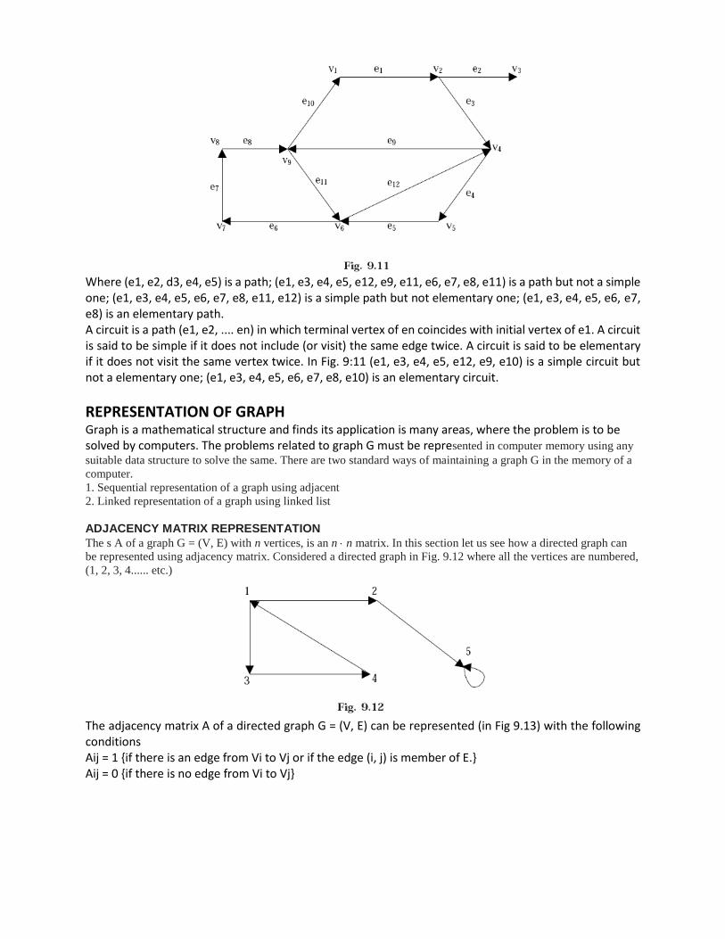
Where (e1, e2, d3, e4, e5) is a path; (e1, e3, e4, e5, e12, e9, e11, e6, e7, e8, e11) is a path but not a simple one; (e1, e3, e4, e5, e6, e7, e8, e11, e12) is a simple path but not elementary one; (e1, e3, e4, e5, e6, e7, e8) is an elementary path. A circuit is a path (e1, e2, .... en) in which terminal vertex of en coincides with initial vertex of e1. A circuit is said to be simple if it does not include (or visit) the same edge twice. A circuit is said to be elementary if it does not visit the same vertex twice. In Fig. 9:11 (e1, e3, e4, e5, e12, e9, e10) is a simple circuit but not a elementary one; (e1, e3, e4, e5, e6, e7, e8, e10) is an elementary circuit.

REPRESENTATION OF GRAPH Graph is a mathematical structure and finds its application is many areas, where the problem is to be solved by computers. The problems related to graph G must be represented in computer memory using any

suitable data structure to solve the same. There are two standard ways of maintaining a graph G in the memory of a

computer.

1. Sequential representation of a graph using adjacent

2. Linked representation of a graph using linked list

ADJACENCY MATRIX REPRESENTATION

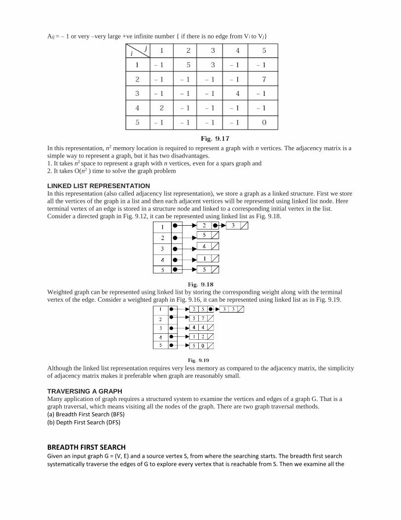
The s A of a graph G = (V, E) with n vertices, is an n n matrix. In this section let us see how a directed graph can

be represented using adjacency matrix. Considered a directed graph in Fig. 9.12 where all the vertices are numbered,

(1, 2, 3, 4...... etc.)

The adjacency matrix A of a directed graph G = (V, E) can be represented (in Fig 9.13) with the following conditions Aij = 1 {if there is an edge from Vi to Vj or if the edge (i, j) is member of E.} Aij = 0 {if there is no edge from Vi to Vj}

We have seen how a directed graph can be represented in adjacency matrix. Now let us discuss how an undirected

graph can be represented using adjacency matrix. Considered an undirected graph in Fig. 9.14

Fig 9.14

The adjacency matrix A of an undirected graph G = (V, E) can be represented (in Fig 9.15) with the following conditions Aij = 1 {if there is an edge from Vi to Vj or if the edge (i, j) is member of E} Aij = 0 {if there is no edge from Vi to Vj or the edge i, j, is not a member of E}

To represent a weighted graph using adjacency matrix, weight of the edge (i, j) is simply stored as the entry in i th row and j th column of the adjacency matrix. There are some cases where zero can also be the possible weight of the edge, then we have to store some sentinel value for non-existent edge, which can be a negative value; since the weight of the edge is always a positive number. Consider a weighted graph, Fig. 9.16

The adjacency matrix A for a directed weighted graph G = (V, E, We ) can be represented (in Fig. 9.17) as

Aij = Wij { if there is an edge from Vi to Vj then represent its weight Wij.}

Aij = – 1 or very –very large +ve infinite number { if there is no edge from Vi to Vj}

In this representation, n2 memory location is required to represent a graph with n vertices. The adjacency matrix is a

simple way to represent a graph, but it has two disadvantages.

1. It takes n2 space to represent a graph with n vertices, even for a spars graph and

2. It takes O(n2 ) time to solve the graph problem

LINKED LIST REPRESENTATION In this representation (also called adjacency list representation), we store a graph as a linked structure. First we store

all the vertices of the graph in a list and then each adjacent vertices will be represented using linked list node. Here

terminal vertex of an edge is stored in a structure node and linked to a corresponding initial vertex in the list.

Consider a directed graph in Fig. 9.12, it can be represented using linked list as Fig. 9.18.

Weighted graph can be represented using linked list by storing the corresponding weight along with the terminal

vertex of the edge. Consider a weighted graph in Fig. 9.16, it can be represented using linked list as in Fig. 9.19.

Although the linked list representation requires very less memory as compared to the adjacency matrix, the simplicity

of adjacency matrix makes it preferable when graph are reasonably small.

TRAVERSING A GRAPH Many application of graph requires a structured system to examine the vertices and edges of a graph G. That is a

graph traversal, which means visiting all the nodes of the graph. There are two graph traversal methods.

(a) Breadth First Search (BFS) (b) Depth First Search (DFS)

BREADTH FIRST SEARCH Given an input graph G = (V, E) and a source vertex S, from where the searching starts. The breadth first search systematically traverse the edges of G to explore every vertex that is reachable from S. Then we examine all the

vertices neighbor to source vertex S. Then we traverse all the neighbors of the neighbors of source vertex S and so on. A queue is used to keep track of the progress of traversing the neighbor nodes. BFS can be further discussed with an example. Considering the graph G in Fig. 9.20

So A, B, C, D, E, F, G, H is the BFS traversal of the graph in Fig. 9.20

ALGORITHM 1. Input the vertices of the graph and its edges G = (V, E)

2. Input the source vertex and assign it to the variable S.

3. Add or push the source vertex to the queue.

4. Repeat the steps 5 and 6 until the queue is empty (i.e., front > rear)

5. Pop the front element of the queue and display it as visited.

6. Push the vertices, which is neighbor to just, popped element, if it is not in the queue and displayed (i.e., not

visited).

7. Exit. DEPTH FIRST SEARCH The depth first search (DFS), as its name suggest, is to search deeper in the graph, whenever possible. Given an

input graph G = (V, E) and a source vertex S, from where the searching starts. First we visit the starting node. Then

we travel through each node along a path, which begins at S. That is we visit a neighbor vertex of S and again a

neighbor of a neighbor of S, and so on. The implementation of BFS is almost same except a stack is used instead of

the queue. DFS can be further discussed with an example. Consider the graph in Fig. 9.20. Suppose the source

vertex is I.

The following steps will illustrate the DFS

Step 1: Initially push I on to the stack.

STACK: I

DISPLAY:

Step 2: Pop and display the top element, and then push all the neighbors of popped element (i.e., I) onto the stack, if

it is not visited (or displayed or not in the stack.

STACK: G, H

DISPLAY: I

Step 3: Pop and display the top element and then push all the neighbors of popped the element (i.e., H) onto top of

the stack, if it is not visited.

STACK: G, E

DISPLAY: I, H

The popped element H has two neighbors E and G. G is already visited, means G is either in the stack or displayed.

Here G is in the stack. So only E is pushed onto the top of the stack.

Step 4: Pop and display the top element of the stack. Push all the neighbors of the popped element on to the stack, if

it is not visited.

STACK: G, D, F

DISPLAY: I, H, E

Step 5: Pop and display the top element of the stack. Push all the neighbors of the popped element onto the stack, if

it is not visited.

STACK: G, D

DISPLAY: I, H, E, F

The popped element (or vertex) F has neighbor(s) H, which is already visited. Then H is displayed, and will not be

pushed again on to the stack.

Step 6: The process is repeated as follows.

STACK: G

DISPLAY: I, H, E, F, D

STACK: //now the stack is empty

DISPLAY: I, H, E, F, D, G

So I, H, E, F, D, G is the DFS traversal of graph Fig 9:20 from the source vertex I.

Algorithm 1. Input the vertices and edges of the graph G = (V, E).

2. Input the source vertex and assign it to the variable S.

3. Push the source vertex to the stack.

4. Repeat the steps 5 and 6 until the stack is empty.

5. Pop the top element of the stack and display it.

6. Push the vertices which is neighbor to just popped element, if it is not in the queue and displayed (ie; not visited).

7. Exit.

MINIMUM SPANNING TREE A minimum spanning tree (MST) for a graph G = (V, E) is a sub graph G1 = (V1, E1) of G contains all the vertices of G. 1. The vertex set V1 is same as that at graph G. 2. The edge set E1 is a subset of G. 3. And there is no cycle. If a graph G is not a connected graph, then it cannot have any spanning tree. In this case, it will have a spanning forest. Suppose a graph G with n vertices then the MST will have (n – 1) edges, assuming that the graph is connected. A minimum spanning tree (MST) for a weighted graph is a spanning tree with minimum weight. That is all the vertices in the weighted graph will be connected with minimum edge with minimum weights. Fig. 9.22 shows the minimum spanning tree of the weighted graph in Fig. 9.21.

Two algorithms can be used to obtain a minimum spanning tree of a connected weighted and undirected graph. 1. Kruskal’s Algorithm 2. Prim’s Algorithm KRUSKAL’S ALGORITHM This is a one of the popular algorithm and was developed by Joseph Kruskal. To create a minimum cost spanning

trees, using Kruskalls, we begin by choosing the edge with the minimum cost (if there are several edges with the

same minimum cost, select any one of them) and add it to the spanning tree. In the next step, select the edge with

next lowest cost, and so on, until we have selected (n – 1) edges to form the complete spanning tee. The only thing

of which beware is that we don’t form any cycles as we add edges to the spanning tree. Let us discuss this with an

example. Consider a graph G in Fig. 9.21 to generate the minimum spanning tree.

The minimum cost edge in the graph G in Fig. 9.21 is 1. If you analyze closely there are two edges (i.e., (7, 3), (4,

9)) with the minimum cost 1. As the algorithm says select any one of them. Here we select the edge (7, 3) as shown

in Fig. 9.23. Again we select minimum cost edge (i.e., 1), which is (4, 9) as shown in Fig. 9.24.

Next we select minimum cost edge (i.e., 2). If you analyze closely there are two edges (i.e., (1, 2), (2, 3), (3, 6)) with

the minimum cost 2. As the algorithm says select any one of them. Here we select the edge (1, 2) as shown in the

above Fig. 9.25. Again we select minimum cost edge (i.e., 2), which is (2, 3) as shown in Fig. 9.26. Next we select

minimum cost edge (i.e., 2), which is (3, 6) as shown in Fig. 9.27.

Next minimum cost edge is (1, 9) with cost 3. Add the minimum cost edge to the minimum spanning tree as shown

in Fig. 9.28. If we analyze, next minimum cost edge is (1, 5) with cost 4. Add the minimum cost edge to the

minimum spanning tree as shown in Fig. 9.29.

Next minimum cost edge is (4, 8) with cost 5. Add the minimum cost edge to the minimum spanning tree as shown

in Fig 9.30.

Above figures shows different stages of Kruskasl’s Algorithm.

ALGORITHM Suppose G = (V, E) is a graph, and T is a minimum spanning tree of graph G.

1. Initialize the spanning tree T to contain all the vertices in the graph G but no edges.

2. Choose the edge e with lowest weight from graph G.

3. Check if both vertices from e are within the same set in the tree T, for all such sets of T. If it is not present, add

the edge e to the tree T, and replace the two sets that this edge connects.

4. Delete the edge e from the graph G and repeat the step 2 and 3 until there is no more edge to add or until the

panning tree T contains (n-1) vertices.

5. Exit

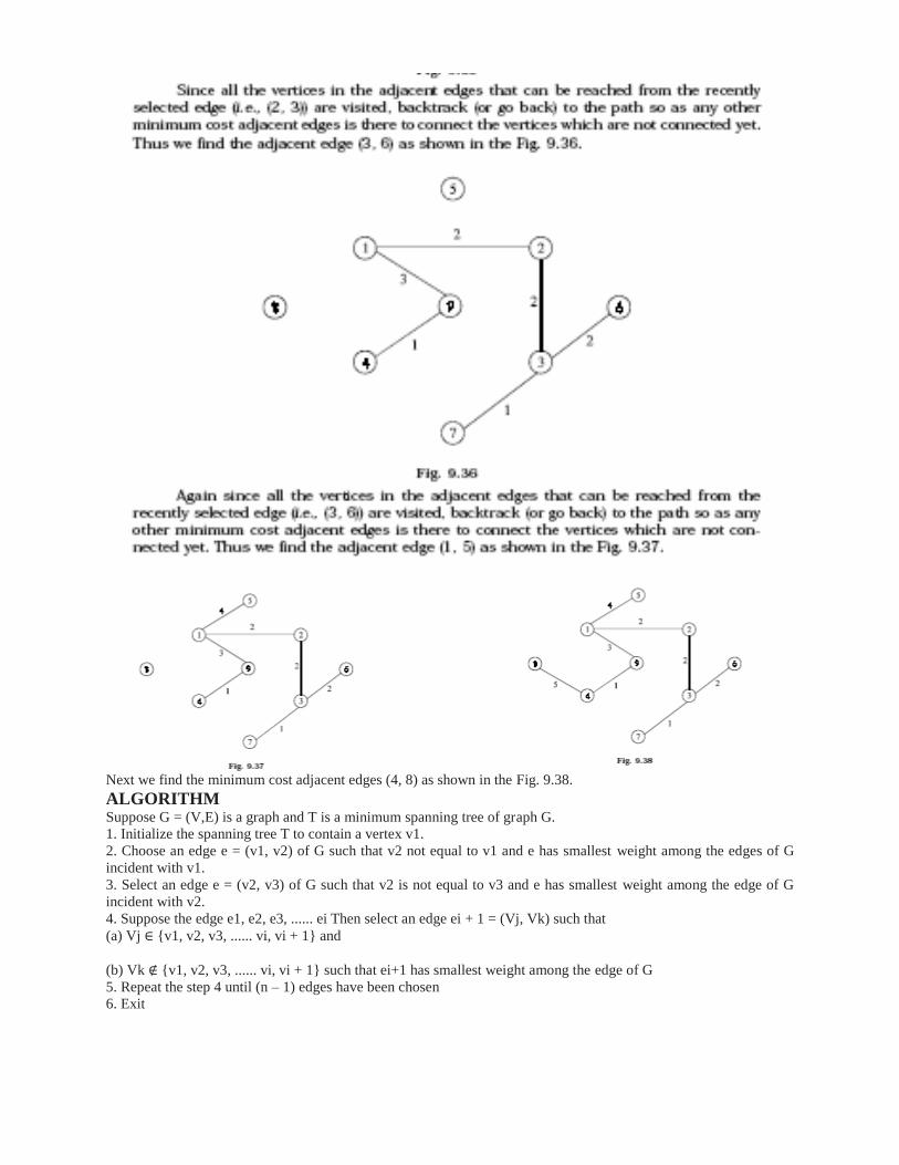
Next we find the minimum cost adjacent edges (4, 8) as shown in the Fig. 9.38.

ALGORITHM Suppose G = (V,E) is a graph and T is a minimum spanning tree of graph G.

1. Initialize the spanning tree T to contain a vertex v1.

2. Choose an edge e = (v1, v2) of G such that v2 not equal to v1 and e has smallest weight among the edges of G

incident with v1.

3. Select an edge e = (v2, v3) of G such that v2 is not equal to v3 and e has smallest weight among the edge of G

incident with v2.

4. Suppose the edge e1, e2, e3, ...... ei Then select an edge ei + 1 = (Vj, Vk) such that

(a) Vj ∈ {v1, v2, v3, ...... vi, vi + 1} and

(b) Vk ∉ {v1, v2, v3, ...... vi, vi + 1} such that ei+1 has smallest weight among the edge of G

5. Repeat the step 4 until (n – 1) edges have been chosen

6. Exit

SHORTEST PATH A path from a source vertex a to b is said to be shortest path if there is no other path from a to b with lower weights.

There are many instances, to find the shortest path for traveling from one place to another. That is to find which route

can reach as quick as possible or a route for which the traveling cost in minimum. Dijkstra's Algorithm is used find

shortest path.

Dijkstra's algorithm solves the single-source shortest-path problem when all edges have non-negative weights. It is a

greedy algorithm and similar to Prim's algorithm. Algorithm starts at the source vertex, s, it grows a tree, T, that

ultimately spans all vertices reachable from S. Vertices are added to T in order of distance i.e., first S, then the

vertex closest to S, then the next closest, and so on. Following implementation assumes that graph G is represented

by adjacency lists.

DIJKSTRA (G, w, s)

1. INITIALIZE SINGLE-SOURCE (G, s)

2. S ← { } // S will ultimately contains vertices of final shortest-path weights

from s

3. Initialize priority queue Q i.e., Q ← V[G]

4. while priority queue Q is not empty do

5. u ← EXTRACT_MIN(Q) // Pull out new vertex

6. S ← S È {u}

// Perform relaxation for each vertex v adjacent to u

7. for each vertex v in Adj[u] do

8. Relax (u, v, w)

Like Prim's algorithm, Dijkstra's algorithm runs in O(|E|lg|V|) time

Step1. Given initial graph G=(V, E). All nodes nodes have infinite cost except the source node, s, which has 0 cost.

Step 2. First we choose the node, which is closest to the source node, s. We initialize d[s] to 0. Add it to S. Relax all nodes adjacent to source, s. Update predecessor (see red arrow in diagram below) for all nodes updated.

Step 3. Choose the closest node, x. Relax all nodes adjacent to node x. Update

predecessors for nodes u, v and y (again notice red arrows in diagram below).

Step 4. Now, node y is the closest node, so add it to S. Relax node v and adjust its predecessor (red arrows remember!).

Step 5. Now we have node u that is closest. Choose this node and adjust its neighbor node v.

Step 6. Finally, add node v. The predecessor list now defines the shortest path from each node to the source node, s.

Warshall’s Algorithm

Let G be directed weighted graph with m nodes v1,v2,…..vm. Suppose we want to find the path matrix P of the graph

G. warshall gave an algorithm for this purpose.

First we define m-square Boolean matrices P0, P1,P2,…..Pm as follows. Let Pk[i,j] denote the ij entry of the matrix

Pk, Then we define :

1 if there is simple path from vi to vj which does not use any other nodes except possibly v1,v2…vk

Pk[i,j] =

0 otherwise

In other words ,

P0[i,j]=1 if there is an edge from vi to vj

P1[i,j]=1 if there is a simple path from vi to vj which does not use any other nodes except possibly v1

P2[i,j]=1 if there is a simple path from vi to vj which does not use any other nodes except possibly v1 and v2.

Here we observe that the matrix P0= A the adjacency matrix of G. and since G has m nodes, the last matrix Pm=P,

the path matrix of G.

Warshall observe that Pk[i,j] =1 can occur only if one of the following two cases occurs:

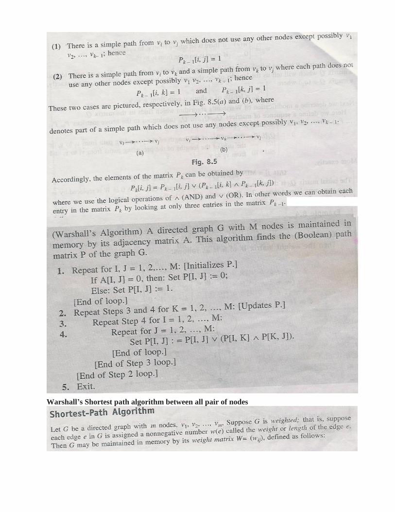
Warshall’s Shortest path algorithm between all pair of nodes

Example