grainsize dynamics of granular flows

Grainsize dynamics of granular flows

BENJAMIN MARKS

B.Sc (Adv), B.Eng (Hons)

Supervisor: Professor Itai EinavAssociate Supervisor: Dr Pierre RognonAssociate Supervisor: Dr Yixiang Gan

A thesis submitted in fulfilment ofthe requirements for the degree of

Doctor of Philosophy

Particles and Grains LaboratorySchool of Civil Engineering

Faculty of EngineeringThe University of Sydney

Australia

29 August 2013

Abstract

This dissertation deals with the description of a granular material as a continuum with an

internal coordinate that represents the grainsize distribution. The inclusion of this internal

coordinate allows us to describe polydispersity in a natural and simple manner.

The bulk of this dissertation is built on four published papers. Each paper is prefaced by

an introductory section, where the motivation for the paper is presented. In the first paper,

I show how the fundamental mechanism of granular segregation can be represented in a

cellular automaton. An equivalent continuum model is derived from the rules of the cellular

automaton, similar to previous theories.

The second paper extends this mechanism to include arbitrary grainsize distributions in

a continuum framework. This continuum description predicts not only the evolution of the

grainsize distribution in space and time, but also the kinematics of the flow. I also show an

extension of the theory in Chapter 5 so that it can be included in a conventional numerical

continuum solver. This is then used to describe steady state grainsize distributions in Chapter

6, where they are shown to be a function of only the stress gradient and diffusivity.

This new continuum theory predicts that segregation will create a lubrication effect that

accelerates the flow. In the third paper, I show experimentally how this lubrication effect

creates additional forces when a granular avalanche impacts a rigid obstacle. At experimental

scale, a 20% increase in force is measured, as compared to a monodisperse avalanche.

In the final paper, comminution is added to the grainsize framework in a new cellular

automaton, allowing me to model crushable flows. I show how the grainsize distributions

measured in confined comminution can be predicted from this model. Additionally, when

segregation is introduced log-normal grainsize distributions develop as in avalanche flow. The

transition from power law to log-normal grainsize distributions is explained as an interaction

between comminution, segregation, and to a lesser extent mixing.

ii

ABSTRACT iii

All of these effects are treated as a direct result of the introduction of the grainsize

distribution. This is a paradigm shift for modelling large deformation granular problems.

Acknowledgements

Firstly, I would like to thank my supervisors, Professor Itai Einav, Dr Pierre Rognon

and Dr Yixiang Gan, without whom I would not have had the constant friendship, guidance,

support and expert knowledge which allowed me to accomplish this work. Secondly, I would

like to thank all four of my parents for providing such essentials as food, education, genes,

money, help, advice, friendship and understanding as I have repeatedly fled the country. Also,

I would to thank my sister Leah for never failing to remind me that I am meant to be working,

not just checking facebook.

At ETH Zürich I would like to thank Professor Sasha Puzrin for his indulgence in allowing

me to visit and conduct experiments, when we both knew that I had no idea what I was doing.

Also many thanks to Aurelio Valaulta for his tireless efforts in sieving, lifting, cleaning

and measuring, which got such great results from the experiment at ETH. At University

College London, I would like to thank everyone in the geomechanics group for their support,

friendship, and free office space. Lastly, I would like to thank everyone in the Eagle’s Nest

Research Centre for the constant supply of coffee, beer and support, even after I abandoned

you all. Twice.

iv

Publications and awards

The following publications have been produced as a result of this PhD:

(1) B. Marks and I. Einav. A cellular automaton for segregation during granular ava-

lanches. Granular Matter, 13(3):211-214, 2011.

(2) B. Marks, I. Einav, and P. Rognon. Polydisperse segregation down inclines: To-

wards degradation models of granular avalanches. In Advances in Bifurcation and

Degradation in Geomaterials, pages 145-151. Springer, 2011.

(3) B. Marks, P. Rognon, and I. Einav. Grainsize dynamics of polydisperse granular

segregation down inclined planes. Journal of Fluid Mechanics, 690:499-511, 2012.

(4) B. Marks, A. Valaulta, A. Puzrin, and I. Einav. Design of protection structures: the

role of the grainsize distribution. In Powders and Grains 2013: Proceedings of the

7th International Conference on Micromechanics of Granular Media. American

Institute of Physics Conference Series, 2013.

(5) B. Marks and I. Einav. The interactions between comminution, segregation and

remixing in granular flows, arXiv:1304.4468, 2013.

The following awards have been received during the course of this thesis:

(1) The Annie B Wilson Prize for Research in Civil Engineering, School of Civil

Engineering, The University of Sydney, 2011

(2) Certificate of Research Excellence, Faculty of Engineering, The University of

Sydney, 2012

v

http://arxiv.org/abs/1304.4468

Contents

Abstract ii

Acknowledgements iv

Publications and awards v

Contents v

List of Figures ix

Chapter 1 Introduction 1

Chapter 2 Literature review 4

2.1 Granular materials . . . . . . . . . . . . . . . . . . . . . . . . . . . . . . . . . . . . . . . . . . . . . . . . . . . . . . . 4

2.1.1 Three phases in one . . . . . . . . . . . . . . . . . . . . . . . . . . . . . . . . . . . . . . . . . . . . . . . . . 5

2.1.2 The microscopic world . . . . . . . . . . . . . . . . . . . . . . . . . . . . . . . . . . . . . . . . . . . . . . 6

2.2 Grainsize . . . . . . . . . . . . . . . . . . . . . . . . . . . . . . . . . . . . . . . . . . . . . . . . . . . . . . . . . . . . . . . 7

2.2.1 Grain size . . . . . . . . . . . . . . . . . . . . . . . . . . . . . . . . . . . . . . . . . . . . . . . . . . . . . . . . . . 8

2.2.2 Polydispersity . . . . . . . . . . . . . . . . . . . . . . . . . . . . . . . . . . . . . . . . . . . . . . . . . . . . . . 10

2.2.3 Grainsize dynamics . . . . . . . . . . . . . . . . . . . . . . . . . . . . . . . . . . . . . . . . . . . . . . . . . 11

2.3 Granular flows . . . . . . . . . . . . . . . . . . . . . . . . . . . . . . . . . . . . . . . . . . . . . . . . . . . . . . . . . . 12

2.3.1 Granular avalanches . . . . . . . . . . . . . . . . . . . . . . . . . . . . . . . . . . . . . . . . . . . . . . . . 15

2.3.2 Constitutive models . . . . . . . . . . . . . . . . . . . . . . . . . . . . . . . . . . . . . . . . . . . . . . . . . 16

2.3.3 Modelling full scale avalanches . . . . . . . . . . . . . . . . . . . . . . . . . . . . . . . . . . . . . . 19

2.3.4 Historical note . . . . . . . . . . . . . . . . . . . . . . . . . . . . . . . . . . . . . . . . . . . . . . . . . . . . . 20

2.4 Segregation . . . . . . . . . . . . . . . . . . . . . . . . . . . . . . . . . . . . . . . . . . . . . . . . . . . . . . . . . . . . . 22

2.4.1 The brazil nut effect . . . . . . . . . . . . . . . . . . . . . . . . . . . . . . . . . . . . . . . . . . . . . . . . 23

2.4.2 Rotating tumblers . . . . . . . . . . . . . . . . . . . . . . . . . . . . . . . . . . . . . . . . . . . . . . . . . . . 24vi

CONTENTS vii

2.4.3 Heap formation. . . . . . . . . . . . . . . . . . . . . . . . . . . . . . . . . . . . . . . . . . . . . . . . . . . . . 25

2.5 Kinetic sieving . . . . . . . . . . . . . . . . . . . . . . . . . . . . . . . . . . . . . . . . . . . . . . . . . . . . . . . . . . 25

2.5.1 Statistical mechanics . . . . . . . . . . . . . . . . . . . . . . . . . . . . . . . . . . . . . . . . . . . . . . . . 27

2.5.2 Continuum models . . . . . . . . . . . . . . . . . . . . . . . . . . . . . . . . . . . . . . . . . . . . . . . . . 28

2.6 Mixing . . . . . . . . . . . . . . . . . . . . . . . . . . . . . . . . . . . . . . . . . . . . . . . . . . . . . . . . . . . . . . . . . 31

2.7 Crushing . . . . . . . . . . . . . . . . . . . . . . . . . . . . . . . . . . . . . . . . . . . . . . . . . . . . . . . . . . . . . . . . 32

2.7.1 Confined comminution . . . . . . . . . . . . . . . . . . . . . . . . . . . . . . . . . . . . . . . . . . . . . . 33

2.7.2 Crushable flows . . . . . . . . . . . . . . . . . . . . . . . . . . . . . . . . . . . . . . . . . . . . . . . . . . . . 36

2.8 Numerical methods . . . . . . . . . . . . . . . . . . . . . . . . . . . . . . . . . . . . . . . . . . . . . . . . . . . . . . 36

2.8.1 Cellular automata . . . . . . . . . . . . . . . . . . . . . . . . . . . . . . . . . . . . . . . . . . . . . . . . . . . 37

2.8.2 Finite volume methods . . . . . . . . . . . . . . . . . . . . . . . . . . . . . . . . . . . . . . . . . . . . . . 38

2.8.3 Discrete element method . . . . . . . . . . . . . . . . . . . . . . . . . . . . . . . . . . . . . . . . . . . . 39

2.9 Summary . . . . . . . . . . . . . . . . . . . . . . . . . . . . . . . . . . . . . . . . . . . . . . . . . . . . . . . . . . . . . . . 40

Chapter 3 Motivation 41

3.1 A dominant mechanism . . . . . . . . . . . . . . . . . . . . . . . . . . . . . . . . . . . . . . . . . . . . . . . . . . 42

3.2 Contribution towards paper . . . . . . . . . . . . . . . . . . . . . . . . . . . . . . . . . . . . . . . . . . . . . . . 43

Paper 1 A cellular automaton for segregation during granular avalanches 43

Chapter 4 Population balance models 48

4.1 Cellular automaton . . . . . . . . . . . . . . . . . . . . . . . . . . . . . . . . . . . . . . . . . . . . . . . . . . . . . . 48

4.2 Continuum description . . . . . . . . . . . . . . . . . . . . . . . . . . . . . . . . . . . . . . . . . . . . . . . . . . . 48


4.4 Post processing . . . . . . . . . . . . . . . . . . . . . . . . . . . . . . . . . . . . . . . . . . . . . . . . . . . . . . . . . . 50

Paper 2 Grainsize dynamics of polydisperse granular segregation down

inclined planes 50

Chapter 5 Bulk, mean and grainsize dynamics 64

5.1 Conservation of mass . . . . . . . . . . . . . . . . . . . . . . . . . . . . . . . . . . . . . . . . . . . . . . . . . . . . 66

5.2 Conservation of momentum. . . . . . . . . . . . . . . . . . . . . . . . . . . . . . . . . . . . . . . . . . . . . . . 67

5.3 Summary of governing equations . . . . . . . . . . . . . . . . . . . . . . . . . . . . . . . . . . . . . . . . . . 68

viii CONTENTS

5.4 Towards numerical implementation of grainsize dynamics . . . . . . . . . . . . . . . . . . . 69

Chapter 6 Steady State Solutions 71

6.1 Continuum description . . . . . . . . . . . . . . . . . . . . . . . . . . . . . . . . . . . . . . . . . . . . . . . . . . . 72

Chapter 7 Chute experiment 75

7.1 Lubrication effect . . . . . . . . . . . . . . . . . . . . . . . . . . . . . . . . . . . . . . . . . . . . . . . . . . . . . . . . 75


Paper 3 Design of protection structures: the role of the grainsize distribution 77

Chapter 8 Comminution during flow 82


Paper 4 The interactions between comminution, segregation and remixing in

granular flows 82

Chapter 9 Conclusion 95

9.1 Future outlook. . . . . . . . . . . . . . . . . . . . . . . . . . . . . . . . . . . . . . . . . . . . . . . . . . . . . . . . . . . 98

Bibliography 100

Appendix A Post processing 113

A1 Volumetric analysis . . . . . . . . . . . . . . . . . . . . . . . . . . . . . . . . . . . . . . . . . . . . . . . . . . . . . . 113

A2 Homogenisation . . . . . . . . . . . . . . . . . . . . . . . . . . . . . . . . . . . . . . . . . . . . . . . . . . . . . . . . . 114

A2.1 Solid fraction . . . . . . . . . . . . . . . . . . . . . . . . . . . . . . . . . . . . . . . . . . . . . . . . . . . . . . 115

A2.2 Average size . . . . . . . . . . . . . . . . . . . . . . . . . . . . . . . . . . . . . . . . . . . . . . . . . . . . . . . 116

A2.3 Standard deviation of size . . . . . . . . . . . . . . . . . . . . . . . . . . . . . . . . . . . . . . . . . . . 116

List of Figures

1.1 Grainsize dynamics. 2

2.1 A sand dune. 5

2.2 Stress patterns in a single grain. 6

2.3 Common sizes. 8

2.4 Polydispersity of granular materials. 10

2.5 Grading curves. 11

2.6 Barchan sand dunes. 13

2.7 Six common flow geometries. 14

2.8 A granular avalanche. 15

2.9 Rheological models. 16

2.10 The brazil nut effect. 23

2.11 Segregation and heap formation. 25

2.12 ABS ® avalanche airbag. 26

2.13 Segregation profiles. 27

2.14 Steady state solutions. 29

2.15 Single grain crushing. 33

2.16 Particle redistribution after crushing. 34

2.17 Gosper’s glider gun. 37

3.1 Comparison of two theories. 41

3.2 Motivation for a cellular automata. 42

5.1 Dynamics hierarchy. 65

5.2 Numerical implementation. 69

6.1 Steady state solution for bidisperse problems. 73

7.1 Factor of safety due to lubrication. 76

ix

CHAPTER 1

Introduction

Granular materials are ubiquitous in our everyday lives, and in our surroundings. These

materials can exist over many orders of magnitude of sizes, from molecules interacting via

electromagnetic forces, to sand and gravel via mechanical interaction and to asteroids, planets

and stars which are governed by gravitational attraction.

The unification of such disparate systems into a single model is obviously a daunting task.

In fact, the key purpose of this dissertation is to describe how such a range of sizes can be

described mathematically, and to model such systems in a unified manner.

Modelling over many orders of magnitude has its limitations. What is considered ‘continuous’

when viewed at the metre scale can appear very different when viewed at the micron scale.

As a first step towards such a grand goal, let us focus our attention on sands and gravels.

This material is chosen because it is a convenient size for experimentation, of the order of

millimetres. Large representative volumes of such particles can be assembled in laboratories,

and they can be treated as a continuum.

Granular materials exhibit all three phases of matter: solid, liquid and gas. When flowing as

a liquid, particles segregate by size. Once this fluid stops flowing, evidence of the patterns

created by the segregation are trapped in the solid phase.

Granular flows are present in mainly geophysical and industrial problems, however many

of their properties are poorly understood. This work aims to increase our understanding of

how the grainsize distribution affects such flows, and to unify the description of size-related

problems in a continuum framework, where the grainsize is treated as an internal coordinate,

as shown in Figure 1.1.

1

2 1 INTRODUCTION

Agglomeration Segregation Crushing Mixing

Open Systems

Grainsize Dynamics

Closed Systems

FIGURE 1.1: Grainsize dynamics. This involves changes in the grainsizedistribution for both open and closed systems. In this dissertation I will discussmixing, segregation and comminution only.

One of the most readily observed effects of grainsize variation in a granular material is its

tendency to segregate during flow. Granular materials segregate for many reasons and under

many conditions. Small differences in size, density, or even surface roughness, can cause the

particles to segregate while flowing. While generally granular materials can be described as a

continuum, and hence as fluids, there is no analogous segregative term in fluid flow.

Traditionally, instances of segregation are analysed separately for different boundary value

problems. No theory has explained segregation quantitatively in multiple geometries, or for

different sized particles. Additionally, the physical size of the particles is generally neglected

in a segregation analysis.

The bulk of the research into segregation is phenomenological in nature, being derived solely

from experimental and numerical investigation. No universal scaling has been found to

explain multiple instances of segregation across the literature.

Another process that often occurs during granular flows is grain crushing. It is well known that

significant grain crushing occurs in a variety of flow situations, such as avalanches, landslides,

debris flows and milling operations. In each of these cases, the grainsize distribution evolves

in space and time as a result of the crushing, altering the constitutive behaviour of the material.

1 INTRODUCTION 3

There are as yet no models to explain how the constitutive parameters and grainsize distribution

are linked in open systems where particles can advect in space. Additionally, there are no

models to track the grainsize distribution in space and time whilst segregation and crushing

occur.

This project aims at solving the second problem, where one wishes to track the evolution

of the grainsize distribution within a flowing material from a variety of processes, such as

segregation, crushing and mixing. In this work, cellular automata are created, which then

inspire continuum models that can represent this behaviour.

This thesis begins with a simple numerical model of granular segregation, explaining the

important physical processes relevant to the phenomenon. Once the physics is well understood,

a rigorous continuum model is developed that describes segregation in terms of changes in

the local grainsize distribution of the material. Experimental evidence of this phenomenon is

then shown, and further refinements to the theory are given. Finally, segregation is coupled

with comminution in another simple numerical model to explain the grainsize distribution

evolution for natural avalanches, landslides and debris flows.

CHAPTER 2

Literature review

And every one that heareth these sayings of mine, and doeth

them not, shall be likened unto a foolish man, which built his

house upon the sand.

— The King James Bible, Matthew 7:26

Around 2000 years ago, when the Bible was first canonized, very little was understood about

granular materials such as sand, and construction was difficult. Fortunately, many advances

have occurred in the field since then. This Chapter gives a summary of the history and

state of the art of granular materials research, in particular focused on segregation during

flows on inclined planes. It also briefly describes some important points concerning mixing,

comminution processing, cellular automata, finite differencing and the discrete element

method.

2.1 Granular materials

Granular materials have a loose definition in the literature. According to some, they are

considered to be systems composed of a large number of particles with a diameter greater

than 1 micron (Gennes 1999). For others, this size constraint is too limiting, and granular

materials exist over all sizes, in essence only limited by the Planck length1. Also, the notion

of energy loss through interactions between particles seems to be a defining characteristic

(Duran 2000).

1Personal communication with Professor Einav.

4

2.1 GRANULAR MATERIALS 5

FIGURE 2.1: A sand dune. The dune is approximately 500 m across, whereasan individual sand grain is about 500 microns. At this scale, we can treat thedune as being a continuous medium. (c wikimedia.org)

In the absence of cohesive forces between particles, the shape of the material at rest will

be determined by that of the container in which it is resting. Even though this is a property

commonly attributed to fluids, these materials exhibit a large number of behaviours and

phenomena which are not present in continuous media.

The prototypical example of a granular material is sand. It is composed of a large number

of small grains that interact to give macroscopic properties, such as in Figure 2.1. In a

conventional fluid, such as water, a single water molecule is approximately 2.75× 10−10 m

long. A droplet of water, the smallest common unit in day to day life, is approximately

500 microns wide, which is roughly 2,000,000 molecules across, or 1021 molecules per

droplet. This is a big number — approximately the number of sand grains on earth (1020

to 1024). When we have small numbers of particles in a system, the discrete nature of the

material becomes more evident.

2.1.1 Three phases in one

The most obvious property which distinguishes a granular material from a solid or fluid

becomes evident when one attempts to pour sand into a container. As mentioned previously,

the material will flow into and fill the container. An astute observer will, however, notice a

critical distinction between what one expects of water and what actually occurs. Once the

material has settled down, the top of the sand will not form a flat surface, as a liquid would,

6 2 LITERATURE REVIEW

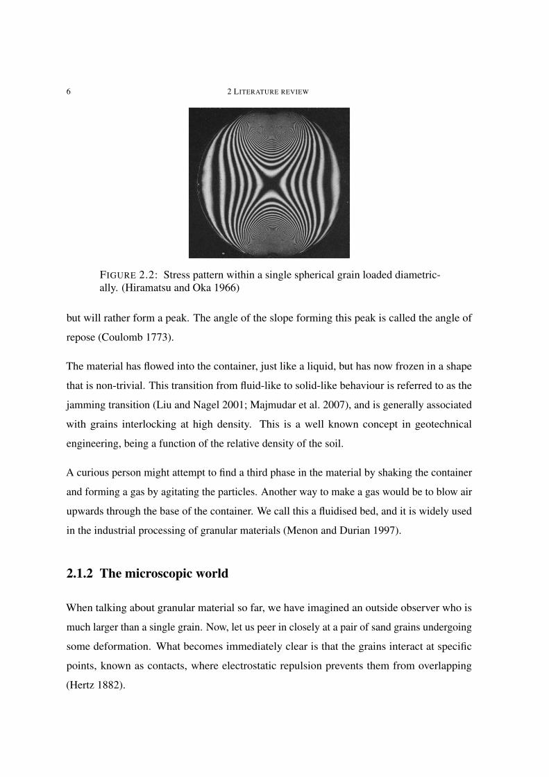
FIGURE 2.2: Stress pattern within a single spherical grain loaded diametric-ally. (Hiramatsu and Oka 1966)

but will rather form a peak. The angle of the slope forming this peak is called the angle of

repose (Coulomb 1773).

The material has flowed into the container, just like a liquid, but has now frozen in a shape

that is non-trivial. This transition from fluid-like to solid-like behaviour is referred to as the

jamming transition (Liu and Nagel 2001; Majmudar et al. 2007), and is generally associated

with grains interlocking at high density. This is a well known concept in geotechnical

engineering, being a function of the relative density of the soil.

A curious person might attempt to find a third phase in the material by shaking the container

and forming a gas by agitating the particles. Another way to make a gas would be to blow air

upwards through the base of the container. We call this a fluidised bed, and it is widely used

in the industrial processing of granular materials (Menon and Durian 1997).

2.1.2 The microscopic world

When talking about granular material so far, we have imagined an outside observer who is

much larger than a single grain. Now, let us peer in closely at a pair of sand grains undergoing

some deformation. What becomes immediately clear is that the grains interact at specific

points, known as contacts, where electrostatic repulsion prevents them from overlapping

(Hertz 1882).

2.2 GRAINSIZE 7

There are a few ways in which these two particles can collide: it is possible for them to slide

past one another, roll over each other, or hit head on. They could of course also undergo any

combination of those collisions. Collision can cause small fragments (asperities) to break off

each other, and degrade the contact points. This can change the local surface conditions and

potentially widen cracks within the grains. These mechanisms are dissipative — the particles

lose energy.

But what happens inside a grain? At each collision, stresses propagate through the grain

(Hiramatsu and Oka 1966). Waves of elastic energy pass through the particle, placing some

areas in compression and other areas in tension, as shown in Figure 2.2. In areas of tension,

cracks are pulled open, weakening the individual grain. If the crack becomes large enough,

the grain can fracture into a collection of small fragments.

Zooming out a little to consider the neighbourhood around the grain, we can observe contact

networks, where loads are transmitted long distances through force chains which branch and

interconnect (Drescher and De Josselin de Jong 1972). Each particle could be in contact with

many other particles – we call this value the coordination number, Z (Smith et al. 1929). If a

grain were to fracture, it would cause nearby particles to rearrange (Russell and Einav 2013),

and change the stress state in the neighbourhood.

2.2 Grainsize

The linear scale, since it was first cut on the wall of an Egyptian temple,

has come to be accepted by man almost as if it were the one unique scale

with which Nature works and builds. Whereas it is nothing of the sort.

Its sole value lies in giving due prominence to the differences and sums

of quantities, when these are what we want to display. But Nature, if she

has any preference, probably takes more interest in the ratios between

quantities; she is rarely concerned with size for the sake of size.

— Ralph A. Bagnold


10−10 10−8 10−6 10−4 10−2 1 102 104 106 108 1010

Representative size of particles, in metres

Molecules

Thin smoke

Haze

Cloud particles

Clouds

MountainsClay

Silt

Atmospheric dust

Dust

Fog particles

Buildings

Vehicles

Boulders

Animals

Gravel

Sand

Cells

Asteroids

Comets

Planets

Stars

Insects

FIGURE 2.3: Common sizes of particles. Adapted from Bagnold (1941).

2.2.1 Grain size

When dealing with particulate matter, we often require a measure of the size of each grain in

the system, or some representative measure of the distribution of sizes. A range of common

sizes are shown in Figure 2.3. There is an inimitable relationship between sizes and scaling

laws. Once we have a definition of a representative size for a particular instance of a class

of bodies, we can then begin to unify our description of that class based on its size, as done

famously in biology in Haldane (1926).

There exist, however, many representative sizes of a particular particle. For a sphere, the

diameter is proportional to the volume cubed. The diameter is also the same as the diameter

of the smallest circular hole through which the particle will pass. If we were to measure the

drag force on the particle falling through a liquid or gas, it would also be directly related to

the diameter. For any other shape, however, all of these quantities may be different. The size

that we measure should be relevant to the physical property which we wish it to describe.

One of the first rigorous characterisation of grain size was done using sieves (Udden 1898).

Depending on the construction of the sieve, a sieve measures either the smallest sphere or

square that a particle can fall through. This size will vary with the sphericity of the particles,

even if the volume remains the same.

2.2 GRAINSIZE 9

A sieve analysis is usually coupled with a hydrometer, in which particles fall through a

liquid, and the time to fall is compared against analytic solutions for spheres. In this way, the

aerodynamic size of the particle is measured, since streamlined particles fall faster than others.

Particle size can also be measured when falling through air (Bagnold 1954). A comprehensive

review of grain size characterisation techniques is given in Syvitski (2007).

Another classical technique is the measurement of individual grains by hand with calipers, to

find quantities such as the maximum, minimum and mean particle diameter (Savage and Lun

1988). This method, however, is sensitive to the operator, and the number of measurements

taken. In fact, repeated handling of materials in this way can often lead to changes in the

surface properties.

A more modern approach to measuring such morphology is to use optical techniques. In

this case, particles can be laid down on a slide and imaged with a microscope, identifying

cross sections of the particles, and properties such as elongation, circularity, aspect ratio and

convexity can be measured rapidly and with a minimal amount of operator error.

Unfortunately, this technique requires the particles to be placed on a slide, which generally

causes them to fall into a stable state such that their principal axis is parallel to the slide. This

can give distorted views of the particles, as they can appear more flat and broad than is truly

representative. To compensate for this, another method was developed in which particles are

allowed to fall past a camera, and images of each grain can be taken of fairly random faces

of the particles (note that particles will preferentially align to reduce wind load, however

tumbling motion does reduce this effect (Goossens 2008)).

A further common method of particle size analysis is to use laser diffraction methods, where

scattered light is analysed to back calculate particle properties (Boer et al. 1987). This method

gives average properties of the medium, rather than individual particle data.

A recent devlopment involves using three dimensional tomography to image the full volume

of each grain (Andò et al. 2012). Using this method, there is no bias from the direction of

imaging. Also, each particle’s surface can be imaged in full. The drawbacks of this method

are the complexity, expense and time that must be taken to image a large number of particles.


FIGURE 2.4: Polydispersity of granular materials. Left: A pile of well sievedgravel. This has a grainsize distribution that is composed of a small range ofsizes, of the order of centimetres. Right: Detritus deposited after a debris flow.The grainsize distribution features every size of particle from clay to boulders,spanning over at least 6 orders of magnitude. (© United States GeologicalSurvey)

After we measure the size of each grain in a sample, there are many ways to convert this data

into a distribution (Folk 1966). Each method gives a particular skew or kurtosis to the data,

especially for small data sets.

2.2.2 Polydispersity

Granular materials are inevitably polydisperse — they are made up of particles of a variety

of sizes. It is difficult to create a sample, even in a laboratory, that has uniform size and

sphericity. Most of the granular materials which we commonly use in our homes, such as flour,

sugar, salt and pepper all have some variety in the size and shape of the constituent grains,

even after careful preparation and manufacturing processes. Naturally occurring granular

materials, such as soils and snow have much larger distributions of sizes, see for example

Figure 2.4.

Polydispersity is one of the greatest elephants in the room of geotechnical engineering. Almost

any geotechnical site investigation begins with a sieve and hydrometer analysis that measures a

grading curve (Bolton 2000), such as shown in Figure 2.5. We take this grading curve, and use

it to define what type of soil we must deal with, typically using the Unified Soil Classification

System (D2487 2011) or some other equivalent model. But then we generally discard the

grading curve for the rest of any analysis, even though we know it to be an important property

2.2 GRAINSIZE 11

10−4 10−3 10−2 10−1 100

Grain diameter (m)

0

20

40

60

80

100

Perc

ent

finer

(%)

FIGURE 2.5: Examples of grading curves. Each line represents the grain sizedistribution of a particular soil sample. The solid line represents a well gradedsample, which is composed of a wide range of particle sizes. The dashed linerepresents a gap-graded, or bidisperse sample, that is mostly composed of justtwo sizes (or at the least missing some sizes in the middle). The dotted linerepresents a uniformly graded, or monodisperse sample, which is composedof grains of a small range of sizes.

of the soil (Zhao et al. 2012; Zhao and Zhang 2013). A vast minority of constitutive models

include as parameters spot measurements from the grading curve, such as taking d50, the

mean diameter (Pouliquen 1999). There is a singular case of a family of models for tracking

changes in the grainsize distribution to model constitutive behaviour (Einav 2007a; Einav

2007b). Two situations where the grading curve is used to good advantage is in the prediction

of permeability (Hazen 1911; Kozeny 1927; Carman 1937; Masch and Denny 1966) and pore

size distribution (Arya and Paris 1981).

2.2.3 Grainsize dynamics

But it is time that we pass to some of the advantages of size.

— JBS Haldane

Generally, we account for the spatial variability of the grain size distribution by applying

different constitutive models in each applicable area. While this is fine for material which

does not advect in space, we often encounter problems where things move, such as in Figure

2.4. For situations where we observe polydisperse materials advecting, we need to account for


the evolution of the grainsize distribution at every point in space. Note that we now change

to grainsize, rather than grain size, to indicate a reference to an internal coordinate which

describes the grain size distribution at every point in space within the material (Marks et al.

2012).

There are many advantages to including a grainsize coordinate in an analysis. Firstly, poly-

disperse materials can be described naturally. Secondly, processes where the grain size

distribution changes, such as milling operations, can be described simply. Thirdly, processes

where the grainsize distribution varies in space, such as segregation, can also be described, in

the same straightforward manner.

Since the analysis uses conventional continuum mechanics, but with an additional coordinate,

we retain all of the advantages of a continuum theory. Motion can be described in terms of

conservation of mass, momentum and energy. Material behaviour can be described using

traditional constitutive models. Scaling laws can be used to simplify the grainsize dynamics.

The possibilities for describing polydisperse granular material using a grainsize coordinate

are wide, varied and exciting. By including a grainsize coordinate in an analysis, the energy

associated with changes in the grainsize distribution can be attributed directly. Once this

energy is known, the dynamics of the grainsize distribution can be described. Then forces,

stresses, displacements and strains can be described in terms of their effect on the grainsize

distribution.

2.3 Granular flows

Flowing granular materials have been studied systematically since 1885 (Reynolds 1885),

however it was only during the second world war that the quantitative study of flowing sand

truly began (Bagnold 1941). Much of this research focused on the interaction of wind and

individual sand grains, and aeolian transport processes, such as in the formation of barchan

dunes, as in Figure 2.6. When particulate matter flows, we say that it is in a liquid state, as

2.3 GRANULAR FLOWS 13

FIGURE 2.6: Barchan sand dunes. Left: A barchan on Earth. Right: Barchandunes on Mars’s Hellespontus region as seen by HiRISE on the Mars Recon-naissance Orbiter. (c wikimedia.org)

opposed to being a solid or gas. This flowing behaviour can occur in many geometries, both

in natural flows and during the industrial processing of granular materials.

We categorise these flows generally by the amount of fluid contained within the pore spaces.

Dry flows are common in industrial manufacturing, rock avalanches, snow (only if it is very

cold — snow melts when sheared (Turnbull 2011)), sand dunes, heap formation, and hopper

filling and discharge.

In nature, things are normally at least a little bit wet. Flows under these conditions are termed

unsaturated. This is a misleading term and should be avoided — try to use partially saturated

if possible. Examples of these flows are landslides, debris flows and snow avalanches at

moderate temperatures, where significant amounts of liquid water exist within the ice matrix.

For these flows, the water is most definitely not distributed uniformly throughout, but is

expelled from the front of the avalanche, which is fairly dry, and accumulates in the tail. The

mechanisms behind this are still unclear (McArdell et al. 2007).

Finally, there are fully saturated, or submerged flows, which occur wholly under water (or

another liquid). An example of these is a submarine landslide, which can devastate sea bed

pipelines and other offshore infrastructure.

The description of granular materials using computational and analytic models is still an

open area of research. This is especially true for flowing granular materials (Iverson 2003).

In the literature there are no well developed constitutive models which represent a broad

variety of behaviours. There is also little consensus as to what experimental or numerical


FIGURE 2.7: Six common flow geometries: (a) plane shear, (b) annular shear,(c) vertical chute, (d) inclined plane, (e) heap flow and (f) a rotating drum.(MiDi 2004)

data can be used to compare against such models (Hutter et al. 2005). Most of the data we

do have comes from discrete element simulations (see 2.8.3) where the assumptions of low

particle stiffness and small numbers of particles are hard to validate experimentally (Cleary

et al. 1998; Bertrand et al. 2005). A seminal paper is MiDi (2004), in which a collection of

experimental and numerical results are published that agree on many aspects of flows in a

variety of geometries (shown in Figure 2.7) for spheres and discs.

We generally treat these flows as being monodisperse — i.e. they are constituted of particles

of similar size. This is done to remove unnecessary complication, and ‘unwanted’ effects,

such as segregation and mixing, that complicate the material behaviour. This is an open

challenge, which will be investigated in Chapter 7.


FIGURE 2.8: The head of an avalanche of gravel passing down an inclinedchute. The flow is from left to right. At the head, particles saltate above thefree surface, while behind in the body of the avalanche a dense flowing layerdominates.

2.3.1 Granular avalanches

Granular avalanches, for example as shown in Figure 2.8, occur frequently on many different

scales (Davies and McSaveney 1999). They are characterised by a dense layer of particles

flowing down an inclined slope under the influence of gravity, with a free surface above. They

may be channelised or free to spread laterally. At large scales, examples are snow avalanches

(Bartelt and McArdell 2009), pyroclastic flows (Branney and Kokelaar 1992), rock avalanches

(Davies and McSaveney 1999), debris flows (Naylor 1980) and submarine (Hampton et al.

1996) or terrestrial landslides (Savage and Hutter 1989). At smaller scales they occur in

hopper filling and discharge (Shinohara et al. 1972), chute flows (Pouliquen 1999) and heap

formation (Khakhar et al. 2001).

At slope inclinations just above the angle of repose of the material, the avalanche may progress

at relatively constant velocity. During flow, gravitational potential energy is dissipated as heat,

sound, friction and plastic deformation of the constituent particles. At high normal stress

or shear strain rate, this can result in particle crushing or ablation. At higher slope angles,

these losses cannot overcome the addition of energy due to gravity, and the avalanche can

accelerate rapidly. At lower angles, the avalanche loses energy and comes to rest.

In natural avalanches, measurements are normally taken of the vertical fall and horizontal

distances travelled, as well as an estimate of the total mass that moved. In large scale

avalanches, an important mechanism that fuels avalanche propagation is erosion, where a

moving avalanche can scour material from beneath it, adding to the mass of the avalanche,


Shear strain rate, γ0

τ0

Shea

rst

ress

,τ

Newtonian fluidBingham plastic

Shear thinning

Shear thickeningHB

FIGURE 2.9: Common rheological models for viscous fluids.

and increasing its runout distance. This is coupled with deposition, as material is left behind

the trailing edge of the avalanche.

Physical modelling of dry granular avalanches usually occurs in the simplest possible geometry

— an inclined chute. This set up involves an inclined plane, usually roughened, and two glass

side walls through which the flow is imaged (Savage and Hutter 1989; Moriguchi et al.

2009). Characterisation of the internal properties of the flow are still in progress (Sanvitale

and Bowman 2012; Hill et al. 2010). Because of this, boundary measurements of the flow

properties are all that are commonly available. Relations between the boundary measurements

have been found, especially for cases where the flow interacts with obstacles (Faug et al. 2009;

Chanut et al. 2010; Moro et al. 2010). For the case of grains submerged in an index matched

fluid, tracer particles can be used to image the internal velocity field in 3D (Wiederseiner et al.

2011b).

2.3.2 Constitutive models

Granular materials are frictional in nature. The response of the material is dependent on both

the particulate nature of the material, and the properties of each individual grain. A first order


description of the material is that proposed by Coulomb, and formalised in the Mohr-Coulomb

model, where the shear stress required to move the material, τ , increases with normal stress,

σ, (Coulomb 1773), as

τ = c+ σ tanφ,

where φ is the friction angle of the material, and c is the apparent cohesion. For a cohesionless

material, if we imagine a block resting on an inclined plane, with slope θ, the block would

begin to slide when the angle of the plane was θ = φ. This can be expressed as

τ

σ= µc,

where µc = tanφ is the critical slope at which sliding begins. Unfortunately, this model

ignores effects that occur as the material begins to speed up — a rate dependency. For

traditional flow problems, the simplest model that addresses this case is that of a Newtonian

fluid

τ = kγ,

where k is the shear viscosity of the fluid. A variety of constitutive models for fluids are

shown in Figure 2.9. For a Newtonian fluid, the viscosity is independent of the applied normal

stress, and is directly proportional to it. If the material gets more viscous the faster it is

stirred, it is called shear thickening. The most common example of such a fluid is oobleck (a

cornstarch and water mixture). If you walk slowly over a pool of oobleck, you will sink into

it, but if you move quickly, you can stay afloat. The opposite condition is if a fluid gets easier

to stir as the stirring speed increases — a shear thinning material, such as blood, ketchup or

syrup. If the material does not flow below a certain shear stress, τ0, it may be a Bingham

plastic — also known as a yield stress fluid (Bingham 1917),


τ = τ0 + kγ.

A good example of a Bingham plastic is toothpaste. You need to squeeze the bottle to build

up a shear stress of τ0 before the toothpaste will start to flow out. If the viscosity also changes

with the shear strain rate, such that it is either shear thickening or shear thinning, it may be

described as a Herschel-Bulkley (HB) fluid (Herschel and Bulkley 1926) where

τ = τ0 + kγn,

and n is a free parameter. By also accounting for the granular nature of the material, and

including the Mohr-Coulomb criterion, we recover a simple description of a granular flow

τ

σ= µc + (Kγ)n, (2.1)

where K is some time scale. This is a moderately robust fluid model of granular material,

known to work for steady flows far from boundaries (Rognon et al. 2007). From observations

of experimental flows of dry granular material, (Bagnold 1954), and validation with discrete

element simulations (Silbert et al. 2001; Lo et al. 2010), it has been shown that material

flowing over a rough base follows the following scaling

γ(z) ∝√

1− z.

This can be derived by considering a lithostatic stress distribution, and an HB fluid model,

as will be shown in Chapter 4. A more sophisticated constitutive model for monodisperse

spheres of diameter d was developed in Pouliquen (1999); Pouliquen and Forterre (2002).

Here the material is controlled by the inertial number I as


τ

σ= µ(I),

I = γd

√σ

ρ,

µ(I) = µc +µ2 − µcI0/I + 1

,

where µ(I) is the friction coefficient, µ2 is the viscosity at high I and I0 is a constant. This

model informs us about the nature of the parameter K from (2.1), and has been shown to

successfully represent monodisperse flow (MiDi 2004). In Weinhart et al. (2012b), the model

was extended to account for variations in slope angle, bed roughness and flow depth. It has

also been extended into three dimensions to model wall effects in an inclined chute geometry

(Jop et al. 2006).

Because of the complexity of granular flows, model materials with known rheology are

often used instead in experiments, to replicate granular flows (Ghemmour et al. 2008). There

are many challenges that lie ahead to create rheological models which represent full scale

avalanches, where the avalanche body can have variable saturation, pore pressure, grainsize

distribution and turbulence.

2.3.3 Modelling full scale avalanches

Current computational modelling of large scale granular avalanches is generally done using a

finite volume solver for the depth-averaged shallow water equations (Christen et al. 2010).

This is an extension to those initially proposed in Savage and Hutter (1989) for granular

avalanche flow.

Because these are depth-averaged equations, they cannot replicate many behaviours that are

intrinsic to avalanches, such as vertically varying shear strain rates or segregation (Armanini

2013). In addition, the model assumes that the terrain has only small curvatures, and so is not

applicable to model impact on structures, or even steep changes in gradients, such as found

on many hillsides (Hutter et al. 2005).


This type of model generally uses either the Voellmy-Salm (Salm 1993) or the Norwegian

NIS (Norem et al. 1988) constitutive model. These models are designed to reliably predict

the runout distance of snow avalanches, rather than to mimic the internal dynamics of an

avalanche. These are engineering approximations of a constitutive model, rather than attempts

to describe the stress-strain behaviour of small representative volumes of the material.

There are many effects which cannot be captured in this class of model (Iverson 2003), such

as steep coarse surge fronts, fine grained tails and lateral levees. These phenomena are largely

due to segregation-induced non-uniformities in the solid components of the avalanche. By

taking a depth-averaged approach, the ability to track these internal flows within the material

is lost.

To tackle this problem directly, and describe the important processes controlling the avalanche

dynamics, the change in grainsize distribution spatially within the avalanche has to be

accounted for. A five-dimensional model, describing space, time, and an internal coordinate

describing the grainsize, are unfortunately all required to model the physical system reliably.

The simplicity gained by depth averaging, and describing the system in just two spatial

dimensions and time, means that we have neglected important physical processes. This is why

current models of granular avalanches largely do not reproduce physical behaviour (Iverson

2003).

2.3.4 Historical note

Snow avalanches are a serious threat, but to ignore the achievements made

in our science between 1960 and 1990 is unfair. During the last catastrophic

avalanche winter in Switzerland (1999), 97% of all hazard maps functioned

as designed. The failure of the remaining 3% was not due to calculation

error (Gruber and Margreth 2001). This is a remarkable achievement and

credit should be given to these earlier researchers. More importantly, this

feat was accomplished without numerical models, without GIS systems,

without considering snow entrainment and without an accurate constitutive


model describing the internal deformation of the flow. Most hazard maps

were prepared with simple avalanche dynamics models based on steady

state flow. No effort was made to track the motion of the avalanche from

initiation to runout. Lateral spreading was accounted for in an easy way.

Maps and historical records were consulted. The question of why this

system worked so well is perhaps the more honest and intriguing scientific

query than blindly stating new differential equations.

— Bruno Salm 2004

There are various reasons why the work contained within this dissertation is vital for predicting

avalanche runout, and I will here attempt to set out some of those reasons in terms of the

effects observed in granular avalanches.

While many aspects of granular avalanches are at this stage only understood phenomenolo-

gically, the bulk of the work in saving lives from avalanches has already been done (Gruber

and Margreth 2001). Such previous methods rely extensively on historical data to find areas

that are subject to avalanches. Unfortunately, it seems that the frequency and location of

avalanches, landslides and debris flows are changing rapidly (Petley 2012), in part because of

anthropogenic climate change, and in part due to changing land usage patterns.

To appreciate fully what is still to be done in terms of increasing safety for people and

property, a distinction needs to be made between predicting the initiation of an avalanche, and

predicting the runout characteristics. We require models of both these phenomena to be able

to give accurate information about safety from avalanches.

This work makes no advances in our understanding of avalanche initiation. With respect to

the runout of an avalanche, however, I will argue that an understanding of the processes that

are involved within an avalanche are highly important. Since we have no way of predicting

accurately the runout distance of any given snow slab movement over arbitrary terrain, we

have no way of gauging the factors of safety embodied in current hazard maps.


By creating models to represent flow behaviours of snow avalanches accurately, we can begin

to reduce the overdesign inherent in existing hazard maps, enhance the abilities of protection

structures, and provide safer, cheaper and more reliable design practices to those of the past.

In Armanini (2013) there is a call to better understand the migration of boulders internally

within debris flows, as these boulders affect dynamic impact of avalanches with structures. A

first step towards understanding this effect is presented in Chapter 7.

It should be borne in mind that this work is in no way limited to snow avalanche modelling.

With regards to the industrial processing of granular materials, efficiency is far from good

(Lowrison 1974). Current models consider the processing of granular materials as an initial

value problem. Given an initial grainsize distribution and a particular grinder or mill, there are

models to produce expected output grainsize distributions. The geometry of the mill, as well

as the physical processes involved in the crushing, are obfuscated by this level of abstraction.

To increase efficiency, we need better models to account for particle crushing as a boundary

value problem.

According to a 2005 NASA technical report, (Wilkinson et al. 2005), there are many aspects

of granular materials research that will need to be advanced significantly to facilitate extrater-

restrial human survival. We do not have models with sufficiently deep understanding to be

able to design mineral transport and processing techniques in variable gravity.

2.4 Segregation

When we have such a mixture of grains that are of different sizes, they have a tendency to

separate when moved. In a packet of cereal, the crumbs are always at the bottom of the box.

In a jar of mixed nuts, the brazil nuts rise to the top (Mobius et al. 2001). In some situations,

this is a useful tool for separating constitutents in a mixture (Kelly and Spottiswood 1982),

but it often causes unwanted demixing, leading to poor quality control (Johanson 1978) and

safety (Muzzio et al. 2002).

2.4 SEGREGATION 23

FIGURE 2.10: The brazil nut effect. After many periods of shaking the system,the particle rises to the top of the material. Left to right: The simulationssnapshots are taken after 0, 10, 30, 40 and 60 shakes. (Rosato et al. 1987)

The phenomenon of segregation has largely been posed historically as an issue affecting the

quality of mineral processing (Williams 1968; Drahun and Bridgwater 1983). Additionally,

the soil formed from flows which have undergone segregation are also commonly observed

in geological deposits as ‘reverse grading’, where material is deposited with large particles

vertically above smaller ones (Bagnold 1954).

Many mechanisms have been found which could lead to segregation, including kinetic sieving,

trajectory segregation, convection and fluidization (McCarthy 2009). These will now be

investigated in more detail for a variety of well known cases of segregation.

2.4.1 The brazil nut effect

For the case of a jar of nuts, as mentioned before, we notice that large particles rise to the top

of the container after being shaken, as shown in Figure 2.10. There have been a variety of

investigations into how this segregation occurs, and a large number of potential mechanisms

have been proposed. It has been shown that the size (Rosato et al. 1987), density (Hong

et al. 2001) and even the background air pressure (Mobius et al. 2001) all contribute to the

segregation dynamics. The segregation has also been shown to be dependent on the convection

cells which form in a cylindrical container (Knight et al. 1993) due to the shaking motion.


This form of segregation has been studied at low gravity, as it is believed to be responsible

for the surface conditions of asteroids (Güttler et al. 2013). As a result, we know that this

segregation velocity is proportional to gravity.

2.4.2 Rotating tumblers

A common industrial operation involves placing a granular material into a rotating tumbler,

such as a front loading tumble dryer. At low rotational speeds, intermittent or continuous

avalanches form at the surface of the granular bed. Magnetic resonance imaging has revealed

that the free surface flow has a linear velocity profile with a maximum at the free surface,

and stops within the bulk (Nakagawa et al. 1993). During flow, there is a tendency to

segregate material by size (Donald and Roseman 1962) or density (Ristow 1994) in the

radial direction, such that one species accumulates near the axis of the drum, and the other

species collects at the circumference. This phenomenon has been studied for a range of

cylinder geometries experimentally (Khakhar et al. 2003) analytically (Prigozhin and Kalman

1998) and numerically (Khakhar et al. 1997), but laws for predicting the rate of segregation

are still phenomenological. At varying fill levels, different patterns of segregation are visible

(Hill et al. 2004), varying from star-shaped to disc-shaped.

Another form of segregation that may occur in rotating tumblers is axial segregation. After

significant rotation of the cylinder, alternating axial bands can form at the surface due to size

or density differences in particles. This is believed to be a result of the difference in angles

of repose of the mediums, which causes them to flow at different rates in the axial direction

(Donald and Roseman 1962). Yanagita (Yanagita 1999) used a three dimensional cellular

automaton to model this phenomenon and was the first to explain the transition from radial to

axial segregation.

MRI imaging has been conducted to validate this work, and view into the bulk of the material,

not merely at the surface (Hill et al. 2010). The work has noted that some axially segregated

regions exist in the bulk without extending to the surface. This implies that axial segregation

may not in fact be driven exclusively by a surface phenomenon.

2.5 KINETIC SIEVING 25

FIGURE 2.11: Steady state solutions of Makse’s heap theory showing twodifferent modes of segregation. The grey particles are larger than the blackparticles. Left: Intermittent avalanches create layers of segregation. Right:Continuous avalanching allows small particles to migrate towards the base ofthe flow. (Makse 1997)

2.4.3 Heap formation

When a granular material is poured onto a flat plane, it does not spread infinitely far from the

point of pouring (as a traditional fluid would), but rather forms a heap, with a characteristic

slope angle over most of the heap, and a logarithmic tail near the plane (Alonso and Herrmann

1996). As the heap forms, progressive avalanches occur at the free surface, disturbing the

top few layers of the pile as they pass. As this intermittent avalanching occurs, two types of

segregation by size, shape or density are commonly observed, as shown in Figure 2.11.

Drahun and Bridgwater (Drahun and Bridgwater 1983) poured a bidisperse mixture into a two

dimensional heap, and watched how avalanches created alternating striations of the different

particles, which was termed stratification. This was further investigated quantitatively by

Koeppe (Koeppe et al. 1998) and explained in detail by Makse (Makse 1997) as a combination

of ‘spontaneous stratification’ and ‘spontaneous segregation’. The stratification was explained

as a result of the difference in the angle of repose of the mixture components. Because of

this difference, one component preferentially avalanches, creating layers of mono-disperse

deposition. The segregation is a bulk movement of the large grains to the bottom of the pile.

2.5 Kinetic sieving

Stay on top to stay alive.

— ABS-Lawinenairbags


FIGURE 2.12: ABS ® avalanche airbag. Deploying this airbag during anavalanche causes you to increase in volume, and rise above the flow, potentiallysaving your life. (ABS-Lawinenairbags 2013)

Many of the above examples of segregation are a result of granular avalanches. While all of

them have been explained either phenomenologically or analytically, there is still no unified

theory to describe all of the size effects as a boundary value problem. This Section deals with

a mechanism of segregation, kinetic sieving, rather than an example of where it is produced

in nature and/or industry.

When a granular material flows, many collisions between particles will occur. After each

collision, the incident particles separate, creating a void space. Over a short time span, this

void grows, until it is filled by another particle. As the void is growing over time, it is more

likely that a small particle will fit into this void than a larger one. Also, there is a preference

for the void to be filled from the direction of the principal stress gradient (generally this is

due to gravity). Because of this void filling effect, there is a net percolation of small particles

in the direction of the principal stress gradient (normally downwards — in the direction of

gravity).

The flow, however, maintains a fairly uniform solid fraction spatially, and so the large particles

are forced in the opposite direction (upwards), balancing the mass flux of small particles


FIGURE 2.13: Concentration profiles of small particles as a function of dis-tance down slope. The concentration profiles are averaged over one third of theflow using splitter plates. 0% and 100% fines lines indicate areas above/belowwhich there are no/only fine particles respectively. (Savage and Lun 1988)

(downwards). This mechanism of small particles filling voids is termed kinetic sieving, and is

believed to be responsible for many types of segregation.

In a snow avalanche, this mechanism is leveraged to save lives by outfitting skiers with airbags

which deploy when submerged in an avalanche, as shown in Figure 2.12. The large volume of

the person/airbag unit (the airbag is generally around 170 L, a human 66 L) causes the person

to rise rapidly through the flow, giving a 91% reduction in mortality rate if used correctly

(Brugger et al. 2007).

2.5.1 Statistical mechanics

In Savage and Lun (1988) two mechanisms are proposed, which, when coupled together,

predict segregation in good agreement with experiments conducted on bidisperse material

flowing down an inclined chute. The first is the ‘random fluctuating sieve’, which is a gravity-

induced flow of particles into the voids below. By arranging the flow into layers, particles

which are above a vacant hole can pass down into it by free falling under gravity. The second

is ‘squeeze expulsion’ whereby particles can become dynamically unequilibriated and be

‘squeezed’ out from their current layer in a random direction. Squeeze expulsion was used as

a mechanism to satisfy overall mass conservation, so the authors deemed its exact physical

nature to be unimportant.


By using a maximum entropy argument to find percolation velocities, Savage and Lun derive

a continuum theory for particle size segregation in inclined chute flow. Their analytic results

are then compared to experimental work done with polystyrene beads over a 1.1 m chute. Two

angles of inclination were tested, 26◦ and 28◦, and for two concentrations of fines, 10% and

15%. These results were found to agree well with the results of the analytic work, although

the experimental results were quite coarse. Instead of tracking individual particles through

the flow (which was impossible at the time), particles were collected in three bins, giving

information on the vertical particle size distribution averaged over one third of the height of

the flow.

The analytic work predicts a 100% fall line (a line above which no small particles are present)

and a finite time for the flow to segregate fully, as well as the segregation pattern, as shown in

Figure 2.13. This is in keeping with the experimental work, but due to the micromechanical

origins of the analysis, extension to other geometries and grainsize distributions is prohibitively

complicated.

2.5.2 Continuum models

The second dominant theory explaining kinetic sieving is that proposed in Dolgunin and

Ukolov (1995) and expanded further in Gray and Thornton (2005). In their paper, a binary

mixture theory is used to formulate a model for kinetic sieving. The model is based on the

idea that each component of the mixture carries a different amount of the overburden stress.

The scaling of this stress between the two species, however, is not explained, but assumed.

Because little is known about the stress scaling between the two components, percolation

velocities are assumed to be constant through the bulk material. They are taken to be

qGT = ±Bg cos θ, where θ is the inclination of the slope, c is some inter-particle friction,

and B is a dimensionless parameter that is intended to account for varying particle size,

roughness and shape. However, it does not account for the interaction between particles

causing segregation, which is governed by the shear strain rate.


FIGURE 2.14: Gray and Thornton’s steady state solutions for four differentvelocity profiles and two different initial concentrations. Left: φ0 = 50%.Right: φ0 = 30%. Top row: plug flow, u = 1. Second row: basal slip,u = 0.5 + z. Third row: simple shear u = z. Bottom row: Bagnold velocityprofile u = 3(1 − (1 − z)2). Sr = 1 for all cases, Sr = 1, i.e. all solutionsfully segregate at x = 1. (Gray and Thornton 2005)

Gray and Thornton define φs and φl as the small and large particle concentrations at any point

in space such that φs + φl = 1. For the case of spatially homogeneous initial conditions, they

use φ0 to indicate the small particle concentration.

A non-dimensional segregation equation is ultimately found in terms of the small particle

concentration φ, the assumed downslope velocity profile u(z), the height z, the time t and the

segregation number Sr, as


∂

∂t(φu) = Sr

∂

∂z(φ(1− φ)),

where Sr is a non dimensional fitting parameter that determines the time for complete

segregation to occur. This equation is then solved for varying initial concentration φ0, varying

velocity field u(z) and segregation number Sr. The theory is used to predict both the time

evolution of the flow and the steady state segregation patterns, as shown in Figure 2.14. The

solution of Gray and Thornton’s advection equation presents three discontinuities in φ for all

shear cases, in the form of shocks. Two of these occur at the top and bottom of the flow, and

propagate towards each other through the medium. Where they meet, the third discontinuity

forms, at the triple point of the flow.

From this point, two separate flows exist, that of exclusively large particles at the top, and

small particles at the bottom. Further research has investigated a dependence of the percolation

velocity on the shear strain rate (May et al. 2010). Also, the competing theory of Savage and

Lun proposes that the percolation velocity is a function of the shear rate, du/dz. Because of

this assumption, Gray and Thornton predict that segregation occurs in plug flow, as shown in

Figure 2.14. Plug flow is a case where the downslope velocity is constant along the height of

the flow, such as in rigid body motion. In this case there is no change in the orientation of

particles with respect to one another, and so no segregation should or can occur.

Figure 2.14 shows how the theory predicts different segregation patterns depending on the

assumed flow velocity and mixture concentrations. Other solutions have been shown for

inhomogeneous initial conditions, and even temporally varying input concentrations. The

model has been extended several times to include a passive liquid phase (Thornton et al.

2006), diffusive remixing (Gray and Chugunov 2006), avalanche fronts (Thornton and Gray

2008; Gray and Kokelaar 2010) and larger numbers of mixture components, which implicitly

represent sizes (Gray and Ancey 2011).

These continuum models have been validated experimentally in Wiederseiner et al. (2011a)

and values for the fitting parameters have been found from numerical tests (Thornton et al.

2012). The stability of such hyperbolic equations has also been studied (Shearer et al. 2008).

2.6 MIXING 31

These continuum theories are dissociated from the bulk behaviour of the material, describing

only the segregation patterns observed during flow. To describe the segregation that occurs

during non-steady flows, the segregation pattern needs to be coupled to the kinematics. In

addition, these continuum models neglect the physical size of the grains in the analysis, and

so have no way of capturing size effects.

The major holes existing in such continuum theories that I wish to address are:

(1) using the physical size of the constituent particles,

(2) inclusion of a constitutive model,

(3) the effect of size contrast on the time for segregation and

(4) modelling arbitrary grainsize distributions.

2.6 Mixing

Another important mechanism in granular flows is mixing. As material flows, random

fluctuations in particle motion occur due to repeated collisions giving rise to mixing. As

with traditional fluids (Fick 1855), we can measure the diffusive flux of some variable T in a

system as

J = −D∇T,

with diffusion coefficient D, which has units length2 per unit time. This is known as Fick’s

first law, and is analogous to Darcy’s law for hydraulics. It is well known that a material made

up of particles undergoing a random walk, or Brownian motion, will reproduce this behaviour

(Einstein 1905).

There are several quantities which are generally represented as diffusive; mass, momentum

and energy. In contaminant transport in gases, mass diffuses through a system without external

forcing. On the other hand, in the mixing presented in this dissertation, momentum diffuses

through the material. In the heat equation, thermal energy diffuses through a medium.


For a granular material, it has been shown in experiments that the diffusion of momentum in

fact varies linearly with shear strain rate (Campbell 1997; Utter and Behringer 2004). This has

ramifications for the flow of granular material down a slope, as shown in Buser and Bartelt

(2009), where the random kinetic energy, associated with the diffusivity, affects the prediction

of velocity profiles in snow avalanches.

The interaction between segregation and mixing has been investigated for the case of inclined

plane flow (Gray and Chugunov 2006). Mixing causes the otherwise perfect segregation to

become diffuse, matching experiments more closely (Wiederseiner et al. 2011a).

2.7 Crushing

A final important process in granular mechanics is that of crushing. When particles are loaded,

they have some finite probability of fragmenting. When this occurs, the mean grainsize

decreases, as a large particle is converted into several fragments. This could occur from

erosion, where the surface is merely ablated, or from industrial comminution processing at

high confining stress which crush the particle.

During any of these events, the specific surface of the material increases, which requires an

input of energy. During industrial comminution, where a target grainsize distribution is to

be produced, there are huge energy demands for the crushing of brittle materials (roughly

3% of global electricity - (Schoenert 1986)). In this situation, it is known that we operate at

exceedingly low efficiency, roughly 0.1% - 1% (Lowrison 1974).

As identified by the larger community, we require methods to model comminution that

describe the evolution of the full grainsize distribution related to the specific boundary value

problem (King 1993; Powell and Morrison 2007). Inadequate models are one of the main

limiting factors in increasing efficiency for one of the world’s most energy hungry industries.

2.7 CRUSHING 33

FIGURE 2.15: A single grain being crushed. The glass bead is loaded dia-metrically until it fragments explosively. A large range of fragment sizes arecreated as a result of the process. (Cataldo 2012)

2.7.1 Confined comminution

Comminution modelling is generally described in three ‘laws’ attributed to Rittinger, (Rittinger

1867), Kick (Kick 1885) and Bond (Bond 1952). These ‘laws’, or more accurately ‘rules of

thumb’ describe the energy required to facilitate comminution. They inform us that the useful

energy consumed in comminution (the part doing the crushing) is proportional to the newly

generated surface area. Secondly, the energy can be related to the change in particle sizes

from input to output. Lastly, the total useful work in breakage is inversely proportional to the

square root of the diameter of the fragment particles.

2.7.1.1 A single grain

A more enlightening viewpoint can be gained by looking at what happens to individual grains

when crushed, as shown in Figure 2.15. The fracture behaviour of many materials and shapes

have been investigated (Yashima et al. 1987; Perfect 1997). We learn from these experimental

studies that there are common fragment size distributions that occur for a given loading

condition and material type. Also, there is a typical crushing stress at which a particle will

crush, which is related to its material, shape and size.

The variability of particle crushing stress was first described using a weakest link analogy

from Weibull et al. (1951). In this case, we must imagine that a pile of grains has been carved

out of a homogeneous material, with homogeneous crack distribution. Larger particles will

have on average more cracks in them, and so will crush at a lower stress. Small particles will

have low probability of containing a large crack, and so will have a higher crushing stress.


FIGURE 2.16: Energy loss from a crushing event. (a) A particle is about tobe crushed. Contact forces are proportional to the line thickness. (b) Someenergy is converted into new surface area. Other energy is lost due to forcerearrangement as new particles must carry the load. (c) Particle rearrangementis a further mode of energy dissipation, causing plastic volumetric dissipationfrom friction. (Einav and Nguyen 2009; Russell and Einav 2013)

The other component of single particle crushing is the fragment size distribution. In general,

this distribution depends on the loading state of the particle, and the material which is being

crushed. If the material is loaded diametrically, as in a Brazillian test, explosive fragmentation

can be observed and a broad fragment size distribution is measured. If, however, the grain is

merely repeatedly sheared lightly, as in an erosion process, the fragment size distribution will

include many new fragments, orders of magnitude smaller than the initial particle, as well as

a single particle almost as large as the initial particle.

2.7.1.2 Collections of grains

To understand the effect of particle crushing on the system behaviour, we must now consider

an assembly of particles. We can imagine that these particles are loaded in such a way that

one or more of the particles is likely to break. The system chooses certain particles to break,

and these will be particles with large tensile stresses developing within them, causing cracks

to open. A simple model to represent which particles will break was presented using a cellular

automaton in Steacy and Sammis (1991). In this model, particles with neighbours of a similar

size are those that will break.

Particles much larger than their neighbours will be surrounded by many contact points, and

will be subject to fairly isotropic loading. These are unlikely candidates to crush. Similarly,

2.7 CRUSHING 35

small particles will be free to move around the pore spaces, and will not carry significant load.

These are also unlikely to crush. Only those particles surrounded by neighbours of a similar

size will be likely to crush. This nearest neighbour model explains much of the nature of

breakage processes, when coupled with the material behaviour predicted from the weakest

link analogy mentioned above.

We find that in the limit of incredibly high confining stress, the system reaches a stable

grainsize distribution, which is power law in nature (Turcotte 1986; Ben-Zion and Sammis

2003; Crosta et al. 2007). The power law distribution is a signature of a system with no

characteristic size, as any size that was preferentially favoured by the system would then have

a higher likelihood of being crushed.

These power law distributions have in fact been shown to also be fractal in nature using

discrete element method simulations (Ben-Nun et al. 2010) and cellular automata (Steacy and

Sammis 1991; McDowell et al. 1996). The characterisation of the behaviour of the system

into just an evolution towards a fractal state is, however, a simplistic view of the system.

When a single particle crushes, it causes rearrangements not only of the nearby particles, but

also of the force network, as shown in Figure 2.16 and described in Einav and Nguyen (2009);

Russell and Einav (2013).

2.7.1.3 A continuum process

There exists a family of constitutive models for granular materials based on degradation of the

grainsize distribution due to breakage (Einav 2007a; Einav 2007b). These breakage mechanics

models use a scalar parameter to describe changes in the grainsize distribution due to crushing,

from its initial grading to an assumed fractal grading, as first proposed in Hardin (1985).

As the grainsize distribution changes, the constitutive behaviour of the material changes,

capturing the mechanism of isotropic hardening directly.

Another means of modelling the evolution of the grainsize distribution is by harnessing

population balance models (Randolph and Ranjan 1977; Peterson et al. 1985; McGrady

and Ziff 1987; Williams 1990). These models describe the evolution of the full grainsize


distribution over time using an internal coordinate. The models require the knowledge of

two terms: the specific breakage rate of each size, and the fragment size distribution from a

crushing event.

The fragment size distribution has been measured in single particle crushing tests under

different loading conditions (Ryu and Saito 1991; Cheong et al. 2004; Cataldo 2012). The

specific breakage rate, however, is generally assumed to be a power law, which obfuscates the

physical processes involved in these models. Because these models require a priori ultimate

grainsize distributions, they do not give us any guidance as to how crushing will behave in

open systems, such as when the material is flowing.

2.7.2 Crushable flows

When grading curves are measured in the field inside avalanche and landslide runout, log-

normal grainsize distributions are often measured, rather than the power law distributions

measured in static tests. These have been measured in the field (Bartelt and McArdell 2009;

Rastello et al. 2011), in experiment (Imre et al. 2010) but have not been predicted in theory.

How the system reaches a log-normal grading is still unknown. Furthermore, how the grainsize

distribution transitions from a power law, with no typical sizes, to a log-normal one, with a

well defined local size, is also unknown. These challenges will be discussed, and a possible

explanation will be provided, in Chapter 8.

2.8 Numerical methods

This dissertation uses three distinct numerical methods. Firstly, cellular automata are described

to explain pattern forming behaviour. Secondly, continuum conservation equations are solved

numerically using the finite volume method. Thirdly, the discrete element method is used

to validate the continuum theory. A brief description of the rationale for the choice of each

method is outlined below.

2.8 NUMERICAL METHODS 37

FIGURE 2.17: Gosper’s glider gun in Conway’s Game of Life. This set upcreates a constant stream of gliders that propagate down and right. Thesefeatures move themselves through the grid. By interacting these gliders witheach other, universal computation can be achieved. (Conway 1970) c

2.8.1 Cellular automata

Fermi often expressed a belief that future fundamental theories in physics

may involve nonlinear operators and equations, and that it would be useful

to attempt practice in the mathematics needed for the understanding of

nonlinear systems. The plan was then to start with the possibly simplest

such physical model and to study the results of the calculation of its long-

time behavior.

— Stanislaw Ulam

Cellular automata are the progenitors of modern computational methods for modelling

physical systems (Wolfram 1986), beginning with Stanislaw Ulam in 1952, who began

investigating discrete cellular automata to study nonlinear waves and solitons with Enrico

Fermi (Ulam 1952; Fermi et al. 1955). Cellular automata generally consist of a regular

cartesian grid of cells which contain binary information in each cell. A simple rule, or set

of rules, is implemented such that the value in each cell evolves due to the values in each

neighbouring cell. A famous example of a cellular automata is Conway’s Game of Life

(Conway 1970), which exhibits a vast array of behaviours. A famous structure, known as


Gosper’s glider gun, is shown in Figure 2.17. This structure creates gliders, or spaceships,

which are self-propelling patterns.

Many cellular automata have been proposed which model phenomena from all branches of

science (Wolfram 2002). Due to the wide applicability of cellular automata to model physical

processes, there is an open field of research aiming to answer the question of whether or

not the real world is in fact merely a cellular automaton (Ilachinski 2001). Efforts are also

underway to model reality using cellular automata (Fredkin 1991), where the universe is fully

discrete. Additionally, some one dimensional cellular automata have been shown to be Turing

complete (Cook 2004) – i.e. they are capable of universal computing.

There are an exceptionally large number of models using cellular automata that are available

in the literature. They have been used extensively in numerous applications in stochastic

problems, neural networks, pattern recognition, HIV drug therapy, reaction-diffusion systems

(Chopard and Droz 1998), fluid dynamics (Margolus et al. 1986) and biology (Ermentrout,

Edelstein-Keshet et al. 1993). For physical modelling, there are also many examples of using

cellular automata to replace partial differential equations, (Chopard and Droz 1998; Bagnoli

1941; Schweitzer and Zimmermann 2001; Deutsch et al. 2005).

2.8.2 Finite volume methods

In the finite volume method (FVM), the governing equations are integrated piecewise over

a mesh of representative volumes. Using these integrals, fluxes can be balanced across the

boundaries of control volumes (LeVeque 2002).

The FVM is generally used exclusively for solving conservation equations, such as those

presented in Chapter 4. This method is widely popular in computational fluid dynamics

software. FVM is especially powerful on coarse nonuniform grids and in calculations where

the mesh moves to track interfaces or shocks.

There are three main ways of handling discontinuities in a solution using FVM (E Ewing

and Wang 2001). The first is to use an algorithm that tracks the discontinuity, and either

2.8 NUMERICAL METHODS 39

refines the mesh locally around it, or somehow forces the solution to remain stable. This is

often problematic because the number and location of discontinuities are often unknown and

variable.

A more refined method is to use Riemann solvers, where a decomposition of the solution

space resolves shocks as characteristic solutions (Godunov 1959). Any solution can then be

treated as a superposition of discontinuities, and stable, accurate solutions can be found. This

method is very good at capturing discontinuities and shocks in a wide variety of computational

fluid dynamics, magnetohydrodynamics and relativistic problems. Unfortunately, the method

is also complex to solve, and numerically highly intensive.

The method I have chosen to use for this dissertation is a third type. In this method, flux

limiters are used to locally switch between two solution schemes (Van Leer 1979). One

solution scheme is highly accurate, and non-dissipative. This is used when small fluxes pass

between control volumes. The other solution scheme is still accurate, but strongly dissipative,

and is only used when large fluxes pass between control volumes. This gives accurate and

stable solutions, that are simple to implement numerically (Kurganov and Tadmor 2000).

2.8.3 Discrete element method

In the study of granular materials, a common method for simulating the particulate behaviour

of the system is the discrete element method (also known as the distinct element method,

discrete particle method or molecular dynamics simulation). In this type of simulation, a

large number of individual grains are modelled, generally as spheres, that interact with one

another. The method itself is not limited to spherical grains, but computational efficiency

generally requires this. There are many implementations of ellipsoids, prisms or any other

shape (Alonso-Marroquin and Wang 2009).

Particles can either be modelled as perfectly rigid, or soft (Luding 2004). For rigid particles,

event driven algorithms are implemented where the system is numerically time stepped from

collision to collision, with some rule governing the interaction at the instant where the particles

touch.


Soft particles are allowed to overlap, and a force is applied counter to the overlap such that

the particles are gradually forced away from one another (Cundall and Strack 1979). The

normal force is modelled either as a linear spring, or using a Hertzian contact (Hertz 1882).

In addition, tangential, sliding and rotational forces can be calculated to satisfy the needs of

a given model. For this dissertation, I have used a soft body model, called SoftDynamics,

written by Dr Pierre Rognon (Rognon and Gay 2008).

2.9 Summary

As I have outlined, there are many compelling reasons for modelling the evolution of the

grainsize distribution. This can be observed in a number of geometries, and for a number of

physical processes. These include:

• segregation models of granular flows with arbitrary grainsize distributions,

• population balance models for crushing that predict final grading curves,

• constitutive models for granular avalanches with varying grainsize distribution,

• general models for flows of material with arbitrary grainsize distributions in three

dimensional space, and

• coupled comminution, segregation and mixing models of granular flows with coupled

constitutive models.

Once these models have been created, we will begin to understand more completely the role

of the grainsize distribution in facilitating physical phenomena that are at the moment only

poorly understood. This is a necessary step towards building useful design tools that treat

granular flows as boundary value problems of governing equations with wide applicability.

CHAPTER 3

Motivation

When an avalanche occurs, we observe a rapidly flowing region of particles near the free

surface. Due to the chaotic and turbulent nature of the flow, there is a large degree of mixing

and redistribution of particles. Because of this, we do not expect the particle size distribution

to change as the avalanche moves downslope.

In a slightly less energetic flow, such as inclined chute flow at moderate angles (i.e. those near

the friction angle of the material), we see what could be termed ‘laminar’ flow of particulate

matter. In these conditions, many interesting phenomena arise. The one studied in this Chapter

is that of particle size segregation via kinetic sieving.

FIGURE 3.1: Comparison of two theories. Position of concentration shocksfor homogeneous initial conditions and two different initial concentrations oflarge particles. Left: φ0 = 50%. Right: φ0 = 10%. Dashed lines are fromSavage and Lun (1988), solid lines are from Gray and Thornton (2005). (Grayand Thornton 2005)

41

42 3 MOTIVATION

Gray and Thornton (2005)

Savage and Lun (1988)

Cellular automata?

FIGURE 3.2: Motivation for a cellular automata. We wish to explain thefundamental behaviour common to two different theories.

3.1 A dominant mechanism

In the field of kinetic sieving, two main theories are those described by Gray and Thornton

(2005) and Savage and Lun (1988). They both describe thin, rapidly flowing avalanches

of bi-disperse mixtures down an inclined chute. Gray and Thornton use a binary mixture

theory to find concentration shocks which define their solutions. Savage and Lun use a

maximum entropy argument to arrive at a method-of-characteristics approach which describes

a concentration profile.

Both of these theories place significant effort into developing complex mechanisms to predict

the time evolution of the patterns formed by segregation. Solutions to these theories, however,

produce similar results, as shown in Figure 3.1.

Because these two theories have different forms and produce similar results, we are interested

to find the common physics that exists in these models. The subset of physics which exists in

both models should allow us to infer the true behaviour of the system, as shown in Figure 3.2.

In both cases, the mechanism responsible for the segregation predicts that a mixture will

de-mix into two areas of uniform particle size. Additionally, the evolution of the system

towards this fully segregated state should be controlled by the kinematics. We wish to find

the simplest model to explain these two phenomena.

3.2 CONTRIBUTION TOWARDS PAPER 43

The work contained within this Chapter aims to describe the phenomenon in its simplest

terms, as a cellular automaton. Finally, I recover a continuum description of the system from

the rule of the cellular automata, which closely matches existing theory.

3.2 Contribution towards paper

In the following paper, published in Granular Matter during my PhD, I was the primary

researcher and author, being supervised by Professor Itai Einav.

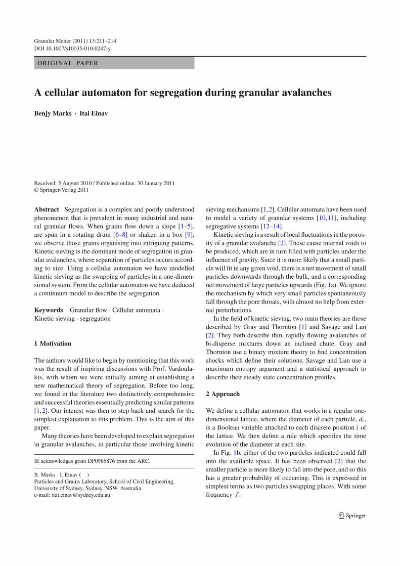
Granular Matter (2011) 13:211–214DOI 10.1007/s10035-010-0247-y

ORIGINAL PAPER

A cellular automaton for segregation during granular avalanches

Benjy Marks · Itai Einav

Received: 5 August 2010 / Published online: 30 January 2011© Springer-Verlag 2011

Abstract Segregation is a complex and poorly understoodphenomenon that is prevalent in many industrial and natu-ral granular flows. When grains flow down a slope [1–5],are spun in a rotating drum [6–8] or shaken in a box [9],we observe those grains organising into intriguing patterns.Kinetic sieving is the dominant mode of segregation in gran-ular avalanches, where separation of particles occurs accord-ing to size. Using a cellular automaton we have modelledkinetic sieving as the swapping of particles in a one-dimen-sional system. From the cellular automaton we have deduceda continuum model to describe the segregation.

Keywords Granular flow · Cellular automata ·Kinetic sieving · segregation

1 Motivation

The authors would like to begin by mentioning that this workwas the result of inspiring discussions with Prof. Vardoula-kis, with whom we were initially aiming at establishing anew mathematical theory of segregation. Before too long,we found in the literature two distinctively comprehensiveand successful theories essentially predicting similar patterns[1,2]. Our interest was then to step back and search for thesimplest explanation to this problem. This is the aim of thispaper.

Many theories have been developed to explain segregationin granular avalanches, in particular those involving kinetic

IE acknowledges grant DP0986876 from the ARC.

B. Marks · I. Einav (B)Particles and Grains Laboratory, School of Civil Engineering,University of Sydney, Sydney, NSW, Australiae-mail: [email protected]

sieving mechanisms [1,2]. Cellular automata have been usedto model a variety of granular systems [10,11], includingsegregative systems [12–14].

Kinetic sieving is a result of local fluctuations in the poros-ity of a granular avalanche [2]. These cause internal voids tobe produced, which are in turn filled with particles under theinfluence of gravity. Since it is more likely that a small parti-cle will fit in any given void, there is a net movement of smallparticles downwards through the bulk, and a correspondingnet movement of large particles upwards (Fig. 1a). We ignorethe mechanism by which very small particles spontaneouslyfall through the pore throats, with almost no help from exter-nal perturbations.

In the field of kinetic sieving, two main theories are thosedescribed by Gray and Thornton [1] and Savage and Lun[2]. They both describe thin, rapidly flowing avalanches ofbi-disperse mixtures down an inclined chute. Gray andThornton use a binary mixture theory to find concentrationshocks which define their solutions. Savage and Lun use amaximum entropy argument and a statistical approach todescribe their steady state concentration profiles.

2 Approach

We define a cellular automaton that works in a regular one-dimensional lattice, where the diameter of each particle, di ,is a Boolean variable attached to each discrete position i ofthe lattice. We then define a rule which specifies the timeevolution of the diameter at each site.

In Fig. 1b, either of the two particles indicated could fallinto the available space. It has been observed [2] that thesmaller particle is more likely to fall into the pore, and so thishas a greater probability of occurring. This is expressed insimplest terms as two particles swapping places. With somefrequency f :

123

212 B. Marks, I. Einav

Fig. 1 Schematics of segregation and corresponding cellular automa-ton rule. Orange are small particles, Blue are large particles. a Effect ofkinetic sieving on particles flowing down an inclined slope. b Two par-ticles attempting to fall into an available space. c The automaton mech-anism, where large and small particles swap places with frequency f . dIndividual simulations are averaged to produce mean model behaviour

di ⇔ di−1 if di < di−1.

Here the double arrow indicates that the variables repre-senting the diameters have swapped positions at cells i andi − 1. Figure 1c illustrates two iterations of the rule on athree particle system. In both cases, the small particles swapwith the large particles, creating segregation. We consider apurely non-diffusive system, in which large particles cannotmove down and small particles cannot move up. We run oursimulation simultaneously in many instances, and averagethe particle diameter at each point across these simulations(Fig. 1d).

We generalise our model with the inclusion of a swap-ping frequency, f , which defines the rate of segregation asa function of the shear strain rate [15] that drives the kineticsieving process, γ . We can then describe the tendency for ourmechanism to occur as a function of the height z such thatf ∝ γ .

The simplest case of flow is that of plug flow, where thedown slope velocity is constant along the depth. For this case,γ = 0 and we expect no segregation. A more complicatedcase is that of simple shear. Here we use a linear velocityprofile, giving us a constant shear rate, and f1 = k where kis a non-dimensional frequency of swapping.

For a more accurate representation of shallow particleflow down an inclined plane, we assume that the shear rate

Fig. 2 Time evolution for two different shear flows. The top rowassumes simple shear, i.e. f1 = k, while the bottom row assumes Bag-nold shear, i.e. f2 = k

√1 − ζ . The system is initially filled with a

mixture of 30 and 80% (left to right) small concentration. Colour barrepresents small particle concentration φ

is approximated by Bagnold shear [16–18], where f2 =k√

1 − ζ , ζ = zH and H is the avalanche depth.

In our model, ζ = iN , where N is the total number of

cells in the vertical direction. We define a non-dimensionaltime τ = j k

N = t kUH . The first equality refers to the cellu-

lar automaton, where j is the time step. The second equalityrefers to the physical time t , where U is the average bulkvelocity across the depth.

The cellular automaton outputs the time evolution of theflow for any applied shear regime and initial mixture. Theflow is described by φ, the small particle concentration. Wefind φ by summing the number of small particles at a givenheight across all of the simulations, and dividing by the totalnumber of simulations.

For a homogeneous initial condition, we start the systemas a randomly generated sample with given concentration ofsmall particles, φ0. As in [12] we begin at the bottom of thesystem, working our way up, checking if each particle hason average smaller particles above it. If it does, it swaps atfrequency f with the above particle. For stability, we workin half time steps, checking only for particles in odd or evenrows. This stops particle from moving many times in a singletime step. The top row is never explicitly checked, but hassmall particles taken out of it by the row below.

3 Results

The top of Fig. 2 shows the behaviour of a system undergo-ing simple shear flow. This is described by f1 = k, i.e. thefrequency is constant over the height. Three sharp concen-tration shocks develop during the time evolution, markingthe boundaries between the two fully segregated states andthe mixed state. The shocks are linear, and move towards adiscrete triple point. The height of this point depends on theinitial concentration of the particles φ.

The bottom of Fig. 2 outlines the case of Bagnold shear,i.e. f2 = k

√1 − ζ . Because of the large swapping frequen-

123

A cellular automaton for segregation during granular avalanches 213

cies at the base of the flow, a concentration shock develops.At the top of the flow, however, the swapping frequency isuniquely zero, and a second concentration shock does notdevelop. In this case, there is no robust definition of com-plete segregation. In a flow of infinite width relative to thegrain size, segregation would never fully occur.

We do not expect a concentration shock at the top of theflow. This is in contrast to suggestion by both Gray andThornton and Savage and Lun. Experimental tests [2,19]generally involve a small number of particles (flows typically10–20 particles deep and with minimal width) and full seg-regation may occur because the problem becomes stochas-tic in nature with insufficient realisations of the segregationstatistics.

When looking at the Bagnold shear case it is evident thatthe small particles saturate the bottom before the large parti-cles saturate the top. Is one faster than the other?

To answer this, we look at a case of heterogeneous initialconditions. We define two regions of mono-disperse parti-cles such that the large particles are below the small par-ticles. The insets of Fig. 3 picture large particles movingupwards through the bulk (3D), and small particles movingdownwards (3B). These two cases correspond to distinctlydifferent aspect ratios between the upper and lower regions,9:1 and 1:9.

We place a ‘gate’ at some height δ, and time until 90%of the contaminating particles have passed beyond this gate.The curves at the right of Fig. 3 plot this time, τ90, for a rangeof values of δ for both simulations. The idea is to present acompetition between the two particles—a race to pass a gateat a similar distance from their initial point.

We see that for any distance moved by the particles, thesmall particles (yellow line) take longer to reach the gate.It should be noted at this stage that we only consider smallsize differences between the two species, and do not accountfor filtration of very small particles through the bulk. Also,the time for one particle to go from the top to the bottom, orthe bottom to the top will be the same. The reason the timesvary in intermediate lengths is due to the asymmetry of theshear strain rate. For example, if the asymmetry was inverted,it would be the smaller particles that trickle faster than thelarge particles float. Using this understanding, it my be pos-sible to tailor industrial processes to obtain faster separationtimes.

4 Continuum model

By averaging over a sufficiently large number of simulations,cellular automaton can be used to represent continuum flowequations [20] by looking at the flux of volume fraction φ

between adjacent cells over time. Over one time step, the fluxthat moves downwards out of a point (ζ, τ ) is the product ofthe swapping frequency at that height f (ζ ), the amount ofthat size present at that height φ(ζ, τ ) and the available spaceto move into. A small particle will only move if it is largerthan the average particle below it and so the available spacecan be expressed as 1 − φ(ζ − �ζ, τ). Taking conservationof mass over a single time step we get:

φ(ζ, τ )�ζ + f (ζ + �ζ)φ(ζ + �ζ, τ)(1 − φ(ζ, τ ))�τ

= φ(ζ, τ + �τ)�ζ + f (ζ )φ(ζ, τ )(1 − φ(ζ − �ζ, τ))�τ

Fig. 3 a An initial configuration of small particles sitting above largeparticles. b These small particles sinking to the bottom of the flow,under Bagnold shear. c An initial configuration of large particles sittingbelow small particles. d These large particles rising to the top of the

flow, under Bagnold shear. e The time for 90% segregation, τ90 at aparticular height δ. The blue line is large particles moving upwards,and the yellow line is small particles moving downwards

123

214 B. Marks, I. Einav

Taking f (ζ ) = kγ , we represent the segregation mecha-nism in terms of the variation of shear strain with height. Incontinuum terms this can be expressed as:

∂φ

∂τ= k

∂(γ φ(1 − φ))

∂ζ

This continuum formula differs from that described byGray and Thornton [1], as it replaces a constant segregationco-efficient Sr with a contribution due to shear strain rate γ .Gray and Thornton’s continuum formulation in one spatialdimension is:

∂φ

∂τ= Sr

∂(φ(1 − φ))

∂ζ

Our model predicts that in a physical flow, such as thatapproximated by Bagnold shear, a concentration shock devel-ops at the bottom of the flow only. The appearance of a shockat the top of the flow is a result of the small number of par-ticles being observed. Flow near the free surface in Bagnoldshear can be approximated by plug flow, corresponding to asituation with extremely slow segregation.

This paper could be viewed in a different light by seeingthe cellular automaton as an effective numerical tool to solvepartial differential equations. These problems are known tobe extremely challenging to solve [21] and such a simpleapproximate solution, which handles shocks and rarefactionswithout qualms, is of great help.

Acknowledgments We would like to thank the members of the Par-ticles, Grains and Complex Fluids Group at the University of Sydney,in particular Dr. Pierre Rognon and Dr. Bjornar Sandnes for useful dis-cussions.

References

1. Gray, J., Thornton, A.: A theory for particle size segregation inshallow granular free-surface flows. Proc. R. Soc. A Math. Phys.Eng. Sci. 461(2057), 1447–1473 (2005)

2. Savage, S., Lun, C.: Particle size segregation in inclined chuteflow of dry cohesionless granular solids. J. Fluid Mech. 189, 311–335 (1988)

3. Gray, J., Hutter, K.: Pattern formation in granular avalanches. Con-tinuum Mech. Thermodyn. 9(6), 341–345 (1997)

4. Naylor, M.: The origin of inverse grading in muddy debris flowdeposits: a review. J. Sediment. Res. 50(4), 1111–1116 (1980)

5. Makse, H., Havlin, S., King, P., Stanley, H.: Spontaneous stratifi-cation in granular mixtures. Nature 386(6623), 379–382 (1997)

6. Nityanand, N., Manley, B., Henein, H.: An analysis of radial segre-gation for different sized spherical solids in rotary cylinders. Met-allurg Trans B 17B, 257 (1986)

7. Khakhar, D., McCarthy, J., Ottino, J.: Radial segregation of gran-ular mixtures in rotating cylinders. Phys Fluids 9, 3600 (1997)

8. Hill, K., Caprihan, A., Kakalios, J.: Bulk segregation in rotatedgranular material measured by magnetic resonance imaging. Phys.Rev. Lett. 78(1), 50–53 (1997)

9. Mobius, M., Lauderdale, B., Nagel, S., Jaeger, H.: Brazil-nut effect:size separation of granular particles. Nature 414(6861), 270 (2001)

10. Baxter, G., Behringer, R.: Cellular automata models of granularflow. Phys. Rev. A 42(2), 1017–1020 (1990)

11. Kozicki, J., Tejchman, J.: Application of a cellular automaton tosimulations of granular flow in silos. Granul. Matter 7(1), 45–54 (2005)

12. Fitt, A., Wilmott, P.: Cellular-automaton model for segregation of atwo-species granular flow. Phys. Rev. A 45(4), 2383–2388 (1992)

13. Yanagita, T.: Three-dimensional cellular automaton model of seg-regation of granular materials in a rotating cylinder. Phys. Rev.Lett. 82(17), 3488–3491 (1999)

14. Cizeau, P., Makse, H., Stanley, H.: Mechanisms of granularspontaneous stratification and segregation in two-dimensionalsilos. Arxiv preprint cond-mat/9809430 (1998)

15. May, L., Shearer, M., Daniels, K.: Scalar conservation laws withnonconstant coefficients with application to particle size segrega-tion in granular flow. J. Nonlinear Sci. 20, 1–19 (2010)

16. Silbert, L.E., Ertas, D., Grest, G.S., Halsey, T.C., Levine, D.,Plimpton, S.J.: Granular flow down an inclined plane: Bagnoldscaling and rheology. Phys. Rev. E 64(5), 051302 (2001)

17. MiDi, G.: On dense granular flows. Eur. Phys. J. E Soft MatterBiol. Phys. 14(4), 341–365 (2004)

18. Rognon, P., Roux, J., Naaim, M., Chevoir, F.: Dense flows of bi-disperse assemblies of disks down an inclined plane. Phys. Fluids19 (2007)

19. Bridgwater, J., Ingram, N.D.: Rate of spontaneous inter-particlepercolation. Chem. Eng. Res. Des. 49a, 163–169 (1971)

20. Toffoli, T.: Cellular automata as an alternative to (rather than anapproximation of) differential equations in modeling physics. Phy-sica D 10(1–2), 117–127 (1984)

21. LeVeque, R.: Finite volume methods for hyperbolic problems.Cambridge University Press, Cambridge (2002)

123

CHAPTER 4

Population balance models

4.1 Cellular automaton

The previous Chapter presented a simple cellular automata. This model was able to replicate

the behaviour of similar continuum and probabilistic theories, and captured the essence

of the segregation mechanism in terms of conservation of mass. To extend the previous

system, this Chapter shows how conservation of momentum can be included in the field

equations describing segregation. It also adds diffusive remixing as a phenomenon which

more accurately represents both physical experiment and numerical simulations.

4.2 Continuum description

In addition to the predictive capability of the cellular automaton, we wish to have access to the

kinematics of the system, while simultaneously describing systems with arbitrary grainsize

distributions. To do this, the model needs to be enriched with a statement of conservation of

momentum.

In the previous cellular automaton, the shear strain rate was shown to govern the evolution of

the segregation patterns. By including conservation of momentum, the segregation patterns

can be directly coupled to the boundary conditions by a constitutive model. Additionally, the

description of the system can be extended to many spatial dimensions.48


To allow arbitrary grainsize distributions, the continuum model is enriched with an internal

coordinate that describes the grainsize distribution explicitly. With this inclusion, the extension

to describe polydisperse systems and their interactions is made simple.

This form of mathematical description is known as a population balance equation (Ramkrishna

2000). This class of equation has been used to describe the conservation of mass of many

particulate systems in chemical and mechanical engineering, and has a very wide applicability

(Ramkrishna and Mahoney 2002). It will be employed here to describe both mass and

momentum conservation of a system of dry grains of arbitrary grainsize distribution.

A population balance model describes the evolution of one or more quantities over time

t, and n spatial dimensions r = {r1, r2, . . . , rn}. Additionally, m internal coordinates,

x = {x1, x2, . . . , xm}, are generally included in the analysis to represent particle size, age,

strength, or any other variable of interest. The general form of a population balance for some

variable f1 is described in (Ramkrishna 2000) as

∂

∂tf1 +∇x · Xf1 +∇r · Rf1 = h. (4.1)

Here the spatial velocities are R, and the velocities in the internal coordinate directions are

X. Additionally, the net birth rate of f1 is h. This balance equation then relates the change

in quantity of f1 due to movement in either an external (spatial) or internal direction, or

due to the spontaneous birth/death of that quantity. To describe the evolution of this system,

this equation must be coupled with some initial and boundary conditions, then solved either

analytically or numerically.


For the following paper, I conducted all of the research and analysis, as well as writing the

paper itself. I was assisted with the discrete element and constitutive modelling by Dr Pierre

Rognon, and in everything else by Professor Itai Einav.

50 4 POPULATION BALANCE MODELS

4.4 Post processing

Detailed post processing routines for the discrete element method are not contained in this

paper, and so have been placed in Appendix A. This Appendix covers how the particulate

data has been homogenised such that data from the whole simulation can be plotted as a

function of either height above an inclined plane, or as a function of grainsize. This method of

homogenisation of polydisperse particulate data is consistent with previous work (Weinhart

et al. 2012a; Thornton et al. 2012).

J. Fluid Mech. (2012), vol. 690, pp. 499–511. c© Cambridge University Press 2011 499doi:10.1017/jfm.2011.454

Grainsize dynamics of polydisperse granularsegregation down inclined planes

Benjy Marks, Pierre Rognon and Itai Einav†

Particles and Grains Laboratory, School of Civil Engineering, The University of Sydney, Sydney,NSW 2006, Australia

(Received 1 July 2011; revised 2 September 2011; accepted 12 October 2011;first published online 14 November 2011)

Granular materials segregate by size when sheared, which increases the destructivepower in avalanches and causes demixing in industrial flows. Here we present aconcise theory to describe this phenomenon for systems that for the first time includeparticles of arbitrary size. The evolution of the grainsize distribution during flow isdescribed based on mass and momentum conservation. The theory is derived in a five-dimensional space, which besides position and time, includes a grainsize coordinate.By coupling the theory with a simple constitutive law we predict the kinematics ofthe flow, which depends on the grainsize dynamics. We show that the underpinningmechanism controlling segregation is a stress variation with grainsize. The theory,solved by a finite difference scheme, is found to predict the dynamics of segregationconsistent with results obtained from discrete element simulations of polydispersegranular flow down inclined planes. Moreover, when applied to bimixtures, the generalpolydisperse theory reveals the role of grainsize contrast.

Key words: granular media, pattern formation, granular mixing

1. IntroductionOne of the most distinct forms of pattern formation in granular materials is that

observable in flows with particles of different size or density. As they flow the grainssegregate, forming complex patterns. This is a concern for industrial applicationswhere generally particles are required to be well mixed. Segregation occurs in flowsdown planes and in rotating cylinders, drums and blenders (Bridgwater 1976; Shinbrot,Alexander & Muzzio 1999; Ottino & Khakhar 2000), which are used for a variety ofapplications in the pharmaceutical, chemical, food, ceramic and construction industries.For a recent comprehensive review of the subject see Gray & Ancey (2011).

It has been noted for some time (Bridgwater & Ingram 1971; Savage & Lun 1988)that segregation down inclined planes occurs due to fluctuations in the local poreswithin the flow, a process termed ‘kinetic sieving’. With increasing shear strain rate,those fluctuations become more frequent. As new void spaces are created and grow,smaller particles are more likely to fit and fall into the pores. This results in a flux ofsmall particles downwards through the bulk and a corresponding flux of large particlesupwards. The segregation velocity, therefore is expected to increase with the rate ofcreation of voids, and therefore with the shear strain rate.

† Email address for correspondence: [email protected]

500 B. Marks, P. Rognon and I. Einav

Here we present a theory that describes this phenomenon for systems that for thefirst time include mixtures of arbitrary sizes. While this topic has been investigated forbimixtures (Savage & Lun 1988; Dolgunin, Kudy & Ukolov 1998; Gray & Thornton2005; Gray & Chugunov 2006; May, Shearer & Daniels 2010), it has only recentlybeen extended to ‘multicomponent’ systems (Gray & Ancey 2011), with n phasesin the mixture. In that theory, particles are ranked from smallest to largest, withoutspecifying the actual radii. Consequently, the number of free parameters increasesquadratically with n, which are grouped into a single function that is not connected tothe actual sizes. In the following section we introduce an alternative continuum theorythat does include the actual sizes using a continuous grainsize coordinate. In § 4.4, wediscuss the fundamental differences of the two approaches.

2. Continuum theoryWe describe an avalanche of depth H, subjected to gravity g, where the largest

particle has radius sM and density ρ0. The following theory is described non-dimensionally. Properties are non-dimensionalized as follows: length by H, grainsizeby sM, time by

√H/g, velocity by

√Hg and stress by ρ0gH.

2.1. A polydisperse mixtureMixtures are generally described by accounting for the various constituents andtheir interactions during flow, such as in Morland (1992). These constituents arecommonly fluids, gases and solids, and a finite number of such constituents are treatedsimultaneously. Here, only solid phases in the flow are considered and we replace thefinite number of constituents with a single grainsize coordinate that maps the grainradii continuously. This allows us to describe a mixture made of arbitrarily sizedsolids. To do this, we introduce a volumetric grainsize distribution φ(r, s, t), of aparticular grainsize s, at some location in space r= {x, y, z} and at time t:

Φ[sa < s< sb] =∫ sb

sa

φ(s′) ds′, (2.1)

where Φ is the solid fraction of grains with grainsize above sa and below sb. Hereφ then represents a probability density function for the grainsize distribution at everypoint in space and time, which satisfies

∫φ ds= 1,

∫φs ds= s, (2.2)

where s(r, t) is the average particle radius.In the following, there is a distinction between intrinsic and partial properties.

Intrinsic properties refer to a particular grainsize, whereas partial properties refer to thecontribution of the intrinsic property of a particular grainsize to the average property.

2.2. DensityThe intrinsic density, ρ∗(s), is defined as the mass of a unit volume of particles withgrainsize s. We allow particles belonging to a particular grainsize s to have differentintrinsic density. Therefore, the partial density, ρ(r, s, t), and the bulk (or average)density, ρ(r, t), are defined as

ρ = φρ∗, ρ =∫ρ ds. (2.3)

Grainsize dynamics of polydisperse segregation 501

2.3. StressStresses are defined in a similar manner to the densities. Accordingly, the intrinsicstress, σ ∗(r, s, t), is the Cauchy stress on the solid part of a representativevolume–grainsize element, meaning an element that refers not only to grains thatbelong to a certain volume in space, but also to a certain grainsize bin. This stresscould be measured, for example using discrete element simulations, as detailed in § 3,where it will be shown to depend on the grainsize. For this reason, we require that theintrinsic stress varies with grainsize s in such a manner that

σ ∗ = σ f , σ = φσ ∗, σ =∫

σ ds, (2.4)

where the intrinsic stress scales about some average, or bulk stress σ (r, t) with scalingf (r, s, t). We also define the partial stress of each constituent, σ (r, s, t). For (2.4) tohold, we require that

∫fφ ds= 1. (2.5)

For a given size s, if f < 1 the intrinsic stress felt by that size is less than the bulkstress, and if f > 1 the intrinsic stress is greater than the bulk stress.

2.4. Conservation of massFollowing Ramkrishna (2000), we define a domain in the particle state space, Λ(t),which contains a finite mass of particles which deforms over time. This domain canbe split into two subdomains containing, first, the external physical space Λr and,second, the internal coordinate space Λs, where s is the grainsize coordinate. With theassumption that no particles enter or leave this domain, i.e. that there is no breakage oragglomeration, we may write in terms of the partial density ρ,

ddt

∫

Λs(t)

∫

Λr(t)ρ dVr ds= 0, (2.6)

where dVr is an infinitesimal physical volume in real space and ds is the equivalentproperty in the grainsize direction. Using a generalization of Reynolds’ transporttheorem to general vector spaces,

∫

Λs(t)

∫

Λr(t)

[∂ρ

∂t+ ∂

∂s(ρS)+∇r · (ρR)

]dVr ds= 0, (2.7)

where S and R are the instantaneous velocities of material ρ in the s and r directions,respectively, and ∇r = {∂/∂x, ∂/∂y, ∂/∂z}. Because the domain of these integrals isarbitrary, and the integral is continuous, we recover the population balance equation ofthe mass in a five-dimensional space {r, s, t}

∂ρ

∂t+ ∂

∂s(ρS)+∇r · (ρR)= 0. (2.8)

We set S = 0, which implies that particles do not grow or reduce over time. Thisis contrasted with Ricard & Bercovici (2009), who explored growth and reductionvia diffusion in grainy materials, where the physical motion of constituents was notexplored. We also make the following assumption

ρR= ρu− D∇rρ, (2.9)


so that the fluxes in physical space are split into two components due to the advectiveflux, ρu, where u(r, s, t)= {u, v,w}, and the diffusive flux, D∇rρ, with some constantdiffusion coefficient D, which we will discuss further in § 3. We can then write

∂ρ

∂t+∇r · (ρu)=∇r · (D∇rρ). (2.10)

Considering a flow that is uniform in the downslope (x) and cross-slope (y)directions, and segregating in the normal (z) direction, we retain a three-dimensionalsystem in {z, s, t}, describing the evolution of the grainsize distribution φ via

∂ρ

∂t+ ∂

∂z(ρw)= D

∂2ρ

∂z2, (2.11)

where it is noted that both ρ and w depend on the grainsize coordinate.

2.5. Conservation of momentumConservation of momentum for our system can be expressed as

ddt

∫

Λs(t)

∫

Λr(t)ρR dVr ds=

∫

Λs(t)

∫

Λr(t)φF∗ dVr ds, (2.12)

where F∗(r, s, t) is the intrinsic force per representative volume–grainsize element. Byagain using Reynolds’ transport theorem, and the arbitrariness of the intergrands,

∂

∂t(ρR)+∇r · (ρR⊗ R)= φF∗, (2.13)

where ⊗ is the outer product. The left-hand side of the equality represents the materialderivative of partial density ρ. Adapting the expressions in Gray & Thornton (2005)and Gray & Chugunov (2006), we set F∗ as

F∗ =−∇r · σ∗ + ρ∗g− ρc

γ(u− u). (2.14)

Note that unlike the work of Gray and colleagues, our definition of the partialforce φF∗ was specified in a way that allows the identification of an intrinsic forceF∗, as was done for density and stress (see § 2.1). Specifically, the first term on theright-hand side represents a force due to the gradient of intrinsic stress. The secondterm represents the intrinsic body force due to gravity g. The final term arises from theinteraction of each species with the bulk. Here u(r, t) = ∫ φu ds and c is a coefficientof interparticle drag, with units of inverse time, to allow normalization by the shearrate γ (r, t). Subsequently, drag force reduces with increasing fluctuation in local porecreation. The exact nature of the parameter c is poorly understood and is thereforetaken as constant. At least, it represents the effects of particle shape, surface roughnessand concavity in terms of their effect on the size segregation velocity.

For simplicity, we assume that the flow is quasisteady, and that the accelerationterms (∂/∂t)(ρR) and ∇r · (ρR⊗ R) can be neglected. This implies that F∗ = 0 with aweak form that can be expressed as

∫ ∫φF∗ dVr ds = 0. From this and (2.2)–(2.5) we

obtain

∇r · σ = ρg. (2.15)

Considering a flow that is uniform in the downslope (x) and cross-slope (y) directions,and without stress at the free surface,

σxz = ρg sin θ(1− z), σzz = ρg cos θ(1− z). (2.16)


Then, after rearrangement, F∗ = 0 becomes

w(s)= γ g cos θc

(f − ρ

∗

ρ

), (2.17)

where we have used the fact that w = 0. This tells us that particles will move relativeto other sizes for two reasons. The first, and the most important for this study, is ifthey feel a partial stress which is different from their neighbours. The second is if theyfeel either a positive or negative buoyancy.

For plug flow, where γ = 0, we expect no segregation to occur because the velocityis constant everywhere and local voids should not be created.

We can now combine our segregation velocity (2.17) with (2.11) to conclude thatour governing population balance equation for grainsize distribution φ is

∂φ

∂t+ g cos θ

c·∂

∂z

(φγ

(f − ρ

∗

ρ

))= D

∂2φ

∂z2. (2.18)

2.6. Constitutive theory

We use a simple constitutive equation that is known to be reasonable for steady,dense flowing granular media down inclines (MiDi 2004; da Cruz et al. 2005), as afirst-order approximation in γ

σxz

σzz= µc + ktiγ , (2.19)

where µc is the angle of repose of our material, k is a non-dimensional constant andti is the inertial time. For quasimonodisperse systems, the inertial time represents thetypical time for a particle to move a distance of its own radius, driven by the normalstress. Rognon et al. (2007) suggested that for bidisperse flows such a behaviour isstill valid provided that the inertial time involves the average size of the mixture, s.Although the precise dependence of the rheology on the polydispersity is still a matterof research (Yohannes & Hill 2010), we shall here employ the simplest hypothesisfor polydisperse mixtures. Following Rognon et al. (2007), we equate the force dueto σzz with the inertial force on a particle of size s with density ρ and a typicalacceleration 2s/t2

i . This gives 4πs2σzz = ρ(4πs3/3) · (2s/t2i ), from which the inertial

time is ti = s√

2ρ/3σzz. Considering the stress profile within a flow down a slope, (see(2.16)) the shear strain rate profile is

γ = tan θ − µc

ks

√3/2g cos θ(1− z). (2.20)

Because s varies with time, the shear strain rate does as well. This impliesthat segregating flows are non-steady, unlike our assumption employed to simplifythe momentum conservation. Nevertheless, we will see in § 3 that this steadinessassumption is already very useful. Introducing this shear strain rate profile in (2.17)provides the segregation velocity as

w= C√

1− zs

(f − ρ

∗

ρ

), (2.21)

where C = (((tan θ − µc)g cos θ)/kc)√(3/2)g cos θ .


g

t 25

t 0

t 12.522°

Peri

odic

BC

Peri

odic

BC

Peri

odic

BC

Peri

odic

BC

Peri

odic

BC

Peri

odic

BC

0 2.7

1.0

0.5z

1.0

1.5

0.51.41.00.6

f

(a) (b)

(c)

FIGURE 1. (Colour online available at journals.cambridge.org/flm) Size segregation in apolydisperse discrete element method (DEM) sample. (a) At t = 0, an initial sample of 1550particles begins flowing downslope. By t = 12.5 the sample has begun to segregate by size,with larger particles collecting at the top of the flow, and smaller particles sinking to thebase. By t = 25 the sample has reached its final segregated state. (b) Bulk vertical stress σzzis shown as a function of height, predicted by (2.16). (c) Size dependence of intrinsic stressexpressed using the scaling function f . We split the simulation into three even layers by depth.The top (O), middle (×) and bottom (�) thirds are shown separately, yet all fit a linear scalinggiven by (3.1). For both right-hand plots, solid lines indicate linear fits to the data.

3. Discrete element method modelLooking at the population balance (2.18), we only require C, D and f to complete

the system. However, this Section demonstrates that the latter two are measurable,leaving C as the only free parameter.

To measure f , we would like to know how the intrinsic stress σ ∗ scales withgrainsize. To do this, we implemented a standard discrete element method (DEM) tosimulate the flow down an inclined plane of a polydisperse mixture of spheres, withs ∈ [0.5, 1] distributed uniformly by volume (see figure 1). As usual, spheres interactby elastic (Hertzian) contacts, with some normal dissipation achieved through adashpot element with coefficient of restitution of 0.6 and tangential friction (coefficientof friction of 0.4). There are 1550 particles in the sample: about 15 large particlediameters deep, 6 wide and 6 long, with periodic boundary conditions in the x andy directions. All of the particles have the same density. The base is a smooth planeinclined at an angle of θ = 22◦. At lower angles, the flow stops; at higher angles,the flow accelerates with increasing diffusion. The plane has some rolling resistance,mimicking roughness, to avoid plug flow (the expression for rolling resistance usedcan be found in Rognon et al. 2010). The particles are initially set randomly with nocontacts, which infers consolidation, and given initial down slope velocities near totheir steady state speeds that are established from a preliminary simulation. Here t = 0is defined when the consolidation has completed (typically at times −0.2 < t < 0).This initial condition was chosen to reach steady state rapidly, before significantsegregation has occurred.


Since we are interested in polydisperse simulations, the numbers of particles withina given grainsize bin is very limited. Therefore, this process was repeated 15 timesand the results were averaged across the simulations, in effect providing nearly 25 000grains.

At a given time t, the intrinsic stress was measured by summing all contact forcesFc acting at contacts c that belonged to particles in depth bin z and grainsize bin s asσ ∗(z, s) ≈ (1/V)∑cFc ⊗ rc where rc is the centre-to-centre vector and V is the totalvolume of particles in that bin. The bin dimensions were selected as small as possiblewhile ensuring sufficient particles in each bin (1z= 0.01,1s= 0.02).

The bulk normal stress was calculated as the volume weighted average of theintrinsic stresses from all bins s at a particular height. As shown in figure 1, it followsthat the bulk normal stress scales as σzz ∝ 1− z, which is consistent with the predictionof (2.16). Moreover, we can measure at different depths the ratio between the intrinsicnormal stress carried by one species σ ∗zz and the bulk stress σzz of all species, to obtainthe function f (see figure 1). It appears that f admits a simple linear scaling with thegrainsize, which is consistent with the requirement discussed in § 2.3

f (r, s, t)= ss. (3.1)

A similar grainsize scaling has been observed during uniaxial compression by Einav(2007), which highlights its significance in polydisperse media.

We also measure the self-diffusion coefficient using the standard expression (see forexample Campbell 1997): D = 〈1z2/21t〉 where 1z represents a change in positionduring an time increment 1t = 0.01. The angle brackets denote an average made overall of the grains, and over some time. While D may in fact be a function of both γand s (Utter & Behringer 2004), for simplicity we only focus here on a constant meanvalue. In these simulations, we measure D ≈ 0.007 (the physical diffusion coefficientnon-dimensionalized by

√H3g).

We can now rewrite (2.18) using (3.1) and (2.21) to give the governing populationbalance equation of polydisperse segregation down inclined planes:

∂φ

∂t+ C

∂

∂z

(φ√

1− zs

(ss− ρ

∗

ρ

))= D

∂2φ

∂z2. (3.2)

Lastly, the only free parameter in our theory, C, was fitted such that the DEMsimulation took the same physical time to reach steady state as the numerical solutionof the continuum theory. The theory can now be implemented in a finite elementcode, because it contains a constitutive model, albeit a simple one. This could also besolved in five-dimensional {r, s, t}-space without the quasisteady assumption, using amore elaborate constitutive model, defined in tensorial form rather than the scalar formemployed in this paper.

4. Results4.1. Solution of governing equation

Solving the governing equation (3.2) is done numerically using a finite differencemethod. Simple methods for solving this class of equation are known to exhibitlarge amounts of numerical dissipation (LeVeque 2002). For that purpose we use aslope-limited total variation diminishing upstream-centred scheme (Quarteroni & Valli1997) to approximate the numerical solution of the general equation in {z, s, t}.


Discrete element method Continuum theory

250

1

z

t 250

1

t0.500.560.610.670.720.780.830.890.941.00

0.500.560.610.670.720.780.830.890.941.00

0.5 1.00

8

0.5 1.0 0.5 1.00

8

0.5 1.0

s

s s s s

0

8

0

8

0

8

0

8

0.5 1.0 0.5 1.0 0.5 1.0 0.5 1.0

0

8

0

8

(a) (b)

FIGURE 2. (Colour online) The DEM system (a) compared with an equivalent solution of thecontinuum theory. (b) Top: spatiotemporal plot of the average grainsize. Remaining: grainsizedistributions at t = 0 (dashed), t = 2 (dash-dotted), t = 5 (dotted) and t = 25 (solid) averagedover different heights of the flow.

The system of equations is solved by discretizing along the z and s directions intoa regularly spaced mesh, and a discretized set of grainsize distribution values φk

i,j isdefined at each height i, grainsize j and time k. The mesh is defined so that the edgesbetween cells lie at the midpoints i± 1/2. Across these edges the total flux is the sumof the fluxes due to the diffusive term (φk

i,jwki,j) and the advective term (−D(∂φk

i,j/∂z))in (3.2). A SuperBee flux limiter is used to minimize dissipation near discontinuities inthe solution, and the resultant numerical flux, h, is constructed from upwinded left andright going fluxes for each φk

i±1/2,j and then projected onto the solution at φk+1i,j . This

can be summarized as

φk+1i,j = φk

i,j −1t1z(hk

i+1/2,j − hki−1/2,j), (4.1)

and the whole scheme can be found in Quarteroni & Valli (1997, pp. 475–481).The solution for all grainsizes are coupled through the dependence of h on s andρ, which are updated each time step by summing over the n discrete grainsizes assk

i =1s∑n

j=1φki,jsj. Lastly, we impose a no flux boundary condition

Cφ√

1− zs

(ss− ρ

∗

ρ

)= D

∂φ

∂zon z= 0, 1. (4.2)


z

u..

1

0 0.5

1

0 0.5u

1

0 0.5

1

0 0.5

Discrete element method Continuum theory(a) (b)

FIGURE 3. The DEM system (a) compared with an equivalent solution of the continuumtheory. (b) For each system, the initial (dashed) and final (solid) shear strain rate anddownslope velocity profiles are shown.

For the results shown here, we have used 1s = 1z = 0.05 and 1t < 1z2. Thisnumerical method has been used extensively for similar problems, such as in Gray& Thornton (2005), and has been shown to be stable and accurate, with a minimalamount of numerical dissipation.

4.2. Results from polydisperse systemOn the left of figures 2 and 3 we represent the time evolution of the DEM sampleshown in figure 1, and the equivalent solution of the analytic theory on the right. Forthat purpose, the theoretical model was solved with the values D = 0.007 (measureddirectly from the DEM in § 3) and C = 0.2 (to match the segregation time).

The theory predicts the grainsize distribution φ(s) at any time of the flow, hereshown for four times, ranging from the initial to final stages. It is clear from bothanalyses that there is significant segregation, which feeds back in a way that intensifiesthe downslope velocity. Also, it appears that at steady state, diffusion prohibitsstratification into layers of uniform grainsizes. Instead, the grainsize distribution has anon-trivial shape that varies with time and position. Nevertheless, the theory predictsqualitative agreement with the DEM realization.

In figure 3, the predictions of the continuum theory for γ and u are compared withthe DEM, which shows comparable shear strain rate next to the basal plane, with bothdecaying strongly towards the free surface. The curvature of the strain rate profile isdifferent. However, this discrepancy is likely related to the linear approximation of theconstitutive law for dry granular flow (2.19). This is also known to be affected by theproximity of the plane (see for instance Rognon et al. 2007).

4.3. Reduction to bimixture theoryThere are many theories describing kinetic sieving in bimixtures. The first such theorywas that of Savage & Lun (1988), where statistical mechanics was employed tomodel the segregation. Later, Dolgunin & Ukolov (1995) and Gray & Thornton (2005)developed continuum models for non-diffusive flow by considering a bimixture withshared solid fraction between the two phases in the flow. More recently, Gray &Chugunov (2006) added diffusion to the previous continuum theories.

For the case of bimixtures, which involve only two distinct grainsizes, with thesame intrinsic density, the grainsize distribution φ can be represented as a polydispersemixture with the help of two dirac δ-functions. For two grainsizes s = {sa, sb} thebidisperse case takes the following grainsize distribution

φ =Φaδ(s− sa)+Φbδ(s− sb), Φa +Φb = 1, (4.3)


ts

C

4

1

0 1

(a) (b)18

0 0.9

FIGURE 4. The time for complete segregation in bidisperse systems. (a) The time as afunction of small grainsize sa, with sb = 1 and Φa = 0.5. The solid line indicates a hyperbolictrend for the segregation time. (b) The time for complete segregation as a function of smallparticle concentration, Φa, for two grainsizes sa = 0.5 and sb = 1.

where Φa and Φb are the solid fractions of the two species. For this case, using (2.17)and (3.1), the segregation velocity of the large particles (s= sb) becomes

w(sb)= γ(

g cos θc

)(sb − sa

s

)(1−Φb), (4.4)

where s= saΦa + sbΦb. Compare this with equation (3.11) of Gray & Thornton (2005):wb = ((Bg cos θ)/c)(1−Φb), where B/c controls the rate of segregation in their model.As in May et al. (2010), our formulation explicitly represents the role of the shearrate. Unlike the previous works of Gray & Thornton (2005) and May et al. (2010),we capture the effects of grainsize difference and the time-dependent local averagegrainsize.

Experiments by Wiederseiner et al. (2011) have shown good agreement withthe theory presented by Gray & Chugunov (2006) for one set of particle sizes(sa = 1 mm, sb = 2 mm). Using this new formulation, it is now possible to explorethe sensitivity of such systems to alternative grainsizes.

We use∫ 1

0

∫ 10 |∂φ/∂t| dz ds 6 0.01 as a criterion for a steady-state solution, applied

for the case of D = 0. Using this definition, in figure 4 we represent this segregationtime, ts, as a function of initial conditions for a variety of bimixtures. On theleft, increasing the size contrast between the particle species reduces the time forsegregation. On the right, for a mixture with grainsize ratio of two, and C = 1, thereis a maximum in the time for segregation at a concentration of approximately 20 %small particles. These results await experimental validation. However, an explanationfor this has already been proposed using a simple cellular automaton, as being due tothe asymmetry of the shear strain rate (Marks & Einav 2011).

4.4. Reduction to multicomponent theoryRecently, Gray & Ancey (2011) proposed a multicomponent theory which extends thework presented in Gray & Thornton (2005) to many dirac δ-functions. For this case,


which involves a discrete number of grainsizes, n, with the same intrinsic density,the grainsize distribution φ can be represented as a sum of dirac δ-functions. Forgrainsizes i = {1, 2, . . . , n} the multicomponent case takes the following grainsizedistribution

φ =n∑

i=1

Φiδ(s− si),

n∑

i=1

Φi = 1, s=n∑

i=1

Φisi, (4.5)

where Φi is the solid fraction of species i, and each i is chosen to perfectly tessellatethe grainsize distribution. For this case, using (2.17) and (3.1), the segregation velocityof grainsize si becomes

w(si)= γ(

g cos θc

)

sin∑

i=1

Φisi

− 1

, (4.6)

which is not immediately comparable to the result produced by Gray & Ancey (2011).As a means of drawing a reasonable comparison, let us specify a geometrical sequencefor the discrete size bins, such as the jth bin being twice the size of the (j − 1)th bin,or sj = s0 · 2j, for some smallest size s0. This set of bin sizes was found to be usefulfor defining grading entropy (Lorincz et al. 2005). Equation (4.6) then becomes

w(si)= γ(

g cos θc

) n∑

j=1

BijΦj, (4.7)

where Bij = (1− 2j−i)/(∑n

m=1Φm2m−i). Similarly, distributing the grainsize bins linearly,sj = s0 + 1s · j, gives Bij = (i − j)/(

∑nm=1Φm((s0/1s) + m)). Compare these with

equations (2.22)–(2.23) of Gray & Ancey (2011), with no diffusion (Dr = 0) wherewi = ((g cos θ)/c)

∑nj=1BijΦj. Gray & Ancey (2011) introduced (1/2)n(n− 1) constants

Bij, as a means to construct analytic solutions. According to our theory thesecoefficients are not constant, but vary with time through Φm. Furthermore, they alsodepend on the allocation of the grainsize bins, which is now obtained naturally byassociating each wi with a grainsize si, without requiring additional parameters.

5. ConclusionsIn this paper we have derived a polydisperse theory for granular segregation, where

we have introduced the notion of a grainsize coordinate. The result of this is a five-dimensional population balance equation. By specifying this for inclined plane flows,this equation simplifies to three dimensions. Pivotal to our theory is the description ofintrinsic stresses that scale with grainsize and control the segregation dynamics. Theuse of a simple constitutive equation that relates the shear stress and the shear strainrate enables us to connect the kinematics to the variation of grainsize distribution. Wepredict a grainsize distribution and a shear strain rate at any time and at any point inspace.

Using this theory we have been able to model the segregation in systems of arbitrarygrainsize distributions. Numerical solutions of the resulting nonlinear populationbalance equation are solved using a finite difference scheme. Comparison has beenmade with DEM simulations and consistent results have been found.


By employing our polydisperse theory to describe segregation in a bidisperse system,we have been able to compare our formulation with previous predictions (Gray &Thornton 2005). In this bidisperse limit, we now understand the role of size contrastbetween the constituents, and how that affects both the time for segregation, and thekinematics of the flow. We have also shown how multicomponent systems can beexpressed in terms of the polydisperse theory, and how the fitting parameters used varywith time and with the choice of grainsize bins.

It is now possible to predict the time for segregation in geophysical and industrialflows and then to tailor conditions to either reduce or increase the extent ofsegregation as necessary. This has relevance for industrial applications that usegranular materials, such as pharmaceutics, agriculture and mining. This can alsoincrease our understanding of long run out landslides, since we predict a shearstrain rate profile, and hence a downslope velocity profile. Also, these dynamics,with the added ingredient of momentum conservation, could be used for the design ofprotection structures.

AcknowledgementsWe would like to thank the members of the Particles and Grains Laboratory at The

University of Sydney. I.E. acknowledges grant DP0986876 from the ARC.

R E F E R E N C E S

BRIDGWATER, J. 1976 Fundamental powder mixing mechanisms. Powder Technol. 15 (2), 215–236.BRIDGWATER, J. & INGRAM, N. D. 1971 Rate of spontaneous inter-particle percolation. Chem.

Engng Res. Des. 49a, 163–169.CAMPBELL, C. S. 1997 Self-diffusion in granular shear flows. J. Fluid Mech. 348, 85–101.DA CRUZ, F., EMAM, S., PROCHNOW, M., ROUX, J-N. & CHEVOIR, F. 2005 Rheophysics of dense

granular materials: discrete simulation of plane shear flows. Phys. Rev. E 72, 021309.DOLGUNIN, V. N. & UKOLOV, A. A. 1995 Segregation modelling of particle rapid gravity flow.

Powder Technol. 83 (2), 95–104.DOLGUNIN, V. N., KUDY, A. N. & UKOLOV, A. A. 1998 Development of the model of

segregation of particles undergoing granular flow down an inclined chute. Powder Technol. 96(3), 211–218.

EINAV, I. 2007 Breakage mechanics – part 1: theory. J. Mech. Phys. Solids 55 (6), 1274–1297.GRAY, J. M. N. T. & ANCEY, C. 2011 Multi-component particle-size segregation in shallow

granular avalanches. J. Fluid Mech. 678, 535–588.GRAY, J. M. N. T. & CHUGUNOV, V. A. 2006 Particle-size segregation and diffusive remixing in

shallow granular avalanches. J. Fluid Mech. 569, 365–398.GRAY, J. M. N. T. & THORNTON, A. R. 2005 A theory for particle size segregation in shallow

granular free-surface flows. Proc. R. Soc. A 461 (2057), 1447–1473.LEVEQUE, R. J. 2002 Finite Volume Methods for Hyperbolic Problems. Cambridge University

Press.LORINCZ, J., IMRE, E., GLOS, M., TRANG, Q. P., RAJKAI, K., FITYUS, S. & TELEKES, G. 2005

Grading entropy variation due to soil crushing. Intl J. Geomech. 5 (4), 311–319.MARKS, B. & EINAV, I. 2011 A cellular automaton for segregation during granular avalanches.

Granul. Matt. 13, 211–214.MAY, L. B. H., SHEARER, M. & DANIELS, K. E. 2010 Scalar conservation laws with non-constant

coefficients with application to particle size segregation in granular flow. J. Nonlinear Sci.1–19.

MIDI, G. D. R. 2004 On dense granular flows. Eur. Phys. J. E 14 (4), 341–365.MORLAND, L. 1992 Flow of viscous fluids through a porous deformable matrix. Surv. Geophys. 13

(3), 209–268.


OTTINO, J. M. & KHAKHAR, D. V. 2000 Mixing and segregation of granular materials. Annu. Rev.Fluid Mech. 32 (1), 55–91.

QUARTERONI, A. & VALLI, A. 1997 Numerical Approximation of Partial Differential Equations.Springer.

RAMKRISHNA, D. 2000 Population Balances: Theory and Applications to Particulate Systems inEngineering. Academic.

RICARD, Y. & BERCOVICI, D. 2009 A continuum theory of grain size evolution and damage.J. Geophys. Res. (Solid Earth) 114 (13), 01204.

ROGNON, P., EINAV, I., BONIVIN, J. & MILLER, T. 2010 A scaling law for heat conductivity insheared granular materials. EPL 89 (5), 58006.

ROGNON, P. G., ROUX, J. N., NAAIM, M. & CHEVOIR, F. 2007 Dense flows of bidisperseassemblies of disks down an inclined plane. Phys. Fluids 19, 058101.

SAVAGE, S. B. & LUN, C. K. K. 1988 Particle size segregation in inclined chute flow of drycohesionless granular solids. J. Fluid Mech. 189, 311–335.

SHINBROT, T., ALEXANDER, A. & MUZZIO, F. J. 1999 Spontaneous chaotic granular mixing.Nature 397, 675–678.

UTTER, B. & BEHRINGER, R. P. 2004 Self-diffusion in dense granular shear flows. Phys. Rev. E 69(3), 031308.

WIEDERSEINER, S., ANDREINI, N., EPELY-CHAUVIN, G., MOSER, G., MONNEREAU, M., GRAY, J.M. N. T. & ANCEY, C. 2011 Experimental investigation into segregating granular flowsdown chutes. Phys. Fluids 23 (1), 013301.

YOHANNES, B. & HILL, K. M. 2010 Rheology of dense granular mixtures: particle-sizedistributions, boundary conditions, and collisional time scales. Phys. Rev. E 82 (6), 061301.

CHAPTER 5

Bulk, mean and grainsize dynamics

In the previous Chapter, a continuum approach was developed so that the grainsize distribution

could be included as an internal coordinate. This was then solved in a single spatial dimension,

and the evolution of the system subject to simple boundary conditions was analysed. For the

future, beyond the scope of this thesis, it is necessary to have a description of the material

that can be included in a numerical analysis.

For this purpose, the mean dynamics must be decoupled from the grainsize dynamics, as

shown in Figure 5.1. This will allow the use of conventional continuum analysis software,

such as the finite element, finite volume or material point methods. To facilitate this, the

current Chapter is devoted to showing how a mean and fluctuation decomposition can be

used to partition the solution space into the mean behaviour of the material and the grainsize

dynamics.

In the field of fluid mechanics, Reynolds decomposition is often used to account for turbulent

behaviour, by averaging over the velocity field to find mean and fluctuating parts (Reynolds

1895). This gives rise to the Reynolds-averaged Navier-Stokes equations, which represent

the time-averaged equations for fluid flow. In this Chapter turbulence is not considered and

fluctuations introduced by the internal coordinate of grainsize create segregation and mixing

instead.

For simplicity, this Chapter treats all of the material as being the same density, so that ρ = φρ.

As a continuum quantity, the intrinsic density of a particular size of particles is defined as

the mass of those particles divided by the volume of tessellated cells surrounding them. This

simplification may not be realistic, as it does not allow changes in volume of the soil skeleton,

64

5 BULK, MEAN AND GRAINSIZE DYNAMICS 65

Mean dynamics

Conservation of mean momentum

(5.11)

Conservation of mean mass (5.9)

Grainsize dynamics

Conservation of mass distribution

(5.10)

Conservation of fluctuation

momentum (5.12)

Bulk dynamics

Conservation of bulk momentum

(5.2)

Conservation of bulk mass (5.1)

FIGURE 5.1: Dynamics hierarchy in the system. The bulk dynamics canbe decomposed into the mean and grainsize dynamics, all of which includeconservation of mass and momentum.

whether due to shearing, compression or grain crushing. This simplification should be relaxed

in further research, and deserves investigation.

To begin, we can split the velocity into a mean u and a fluctuating part u as u = u + u,

where u =∫φuds. The bulk material will move with velocity u, and we can track this mean

component of the dynamics with a traditional continuum solver. The other component, the

grainsize dynamics, must be tracked separately. As shown in Chapter 4, conservation of bulk

mass and momentum can in this case be written as

∂ρ

∂t+∇ · (ρu) +∇ · (ρu) = 0, (5.1)

D

Dt(ρu) +

D

Dt(ρu) = ρg − φf∇ · σ −Dρ∇φ− φρcu

γ. (5.2)

It should be noted that the diffusion term is now included in the momentum equation, rather

than in conservation of mass. As there is no longer an assumption of steady state flow, it

cannot be assumed that diffusion is independent of velocity. Additionally, the term f has been

66 5 BULK, MEAN AND GRAINSIZE DYNAMICS

moved outside of the stress gradient, to be more consistent with Darcy’s law, such that the

system is not driven by partial pressure gradients (Bear 1972).

5.1 Conservation of mass

The purpose of this Section is to split (5.1) into two equations. The first will represent

conservation of mass of the material, and the second will describe the evolution of the

grainsize distribution. If we integrate (5.1) over the grainsize direction s we get

∫∂ρ

∂tds+

∫∇ · (ρu) ds+

∫∇ · (ρu) ds = 0,

or by introducing the integrals into the differentiation and using the fact that∫φu ds = 0,

∂ρ

∂t+∇ · (ρu) = 0, (5.3)

which represents the mean conservation of mass without a grainsize direction. Expanding

(5.1) and using (5.3), and subsequently applying the product rule gives

ρ∂φ

∂t= φ∇ · (ρu)−∇ · (ρφu)−∇ · (ρφu). (5.4)

Applying the product rule again we can state that

∇ · (ρφu) = φ∇ · (ρu) + ρu · ∇φ,

or by rearrangement

φ∇ · (ρu)−∇ · (ρφu) = −ρu · ∇φ.

Putting this in (5.4) gives

5.2 CONSERVATION OF MOMENTUM 67

∂φ

∂t+ u · ∇φ = −1

ρ∇ · (ρφu). (5.5)

This gives us a description of the evolution of the grainsize distribution as a function of

its material derivative. The term on the right hand side will cause changes in the grainsize

distribution due to material flowing at the fluctuation velocity, and not at the mean velocity.

We have partially decoupled the mean mass conservation (5.3) and the mass distribution

conservation (5.5).

5.2 Conservation of momentum

To complete the description of the system in a decoupled state, we can now express the

momentum equations in the same mean and fluctuation decomposition. Integrating (5.2) over

all sizes

∫D

Dt(ρu) ds+

∫D

Dt(ρu) ds =

∫ρg ds−

∫φs

s∇ · σ ds−

∫Dρ∇φ ds−

∫φρcu

γds.

By again moving the integrals into the differentiation, this reduces to

D

Dt(ρu) = ρg −∇ · σ. (5.6)

This is the traditional conservation of mean momentum statement solved for in numerical iner-

tial methods. The final expression required to close the system is a statement of conservation

of fluctuation momentum. To derive this, we can use the product rule to state that

D

Dt(φρu) =

Dφ

Dt· ρu +

D

Dt(ρu) · φ. (5.7)

Substituting (5.6) into this equation gives


D

Dt(φρu) =

Dφ

Dt· ρu + φρg − φ∇ · σ, (5.8)

and putting this into the previous conservation of momentum (5.2) gives, after rearrangement

D

Dt(ρu) = (1− s

s)∇ · σ − Dρ

φ∇φ− ρcu

γ− ρuDφ

Dt.

which represents conservation of fluctuation momentum, only weakly coupled to the mean

dynamics. The first term on the right hand side is the splitting of the mean stress across the

grainsize distribution, giving gradients in space and the grainsize direction. The second term

is the diffusive momentum, which causes remixing of particles to minimise spatial gradients

in the grainsize distribution. The third term is a drag force, creating an interaction between the

sizes, as introduced in Chapter 4. The final term is a convective term, describing the change

in fluctuation momentum due to mean movement of the material.

5.3 Summary of governing equations

We now have four governing equations, two for mass and two for momentum. They are

∂ρ

∂t+∇ · (ρu) = 0, (5.9)

∂φ

∂t+ u · ∇φ+

1

ρ∇ · (ρφu) = 0, (5.10)

D

Dt(ρu) = ρg −∇ · σ, (5.11)

D

Dt(ρu) = (1− s

s)∇ · σ − Dρ

φ∇φ− ρcu

γ+ u∇ · (ρφu). (5.12)

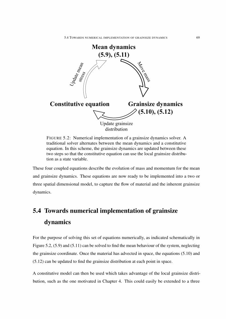
5.4 TOWARDS NUMERICAL IMPLEMENTATION OF GRAINSIZE DYNAMICS 69

Mean dynamics (5.9), (5.11)

Grainsize dynamics (5.10), (5.12)

Constitutive equation

Update grainsize distribution

FIGURE 5.2: Numerical implementation of a grainsize dynamics solver. Atraditional solver alternates between the mean dynamics and a constitutiveequation. In this scheme, the grainsize dynamics are updated between thesetwo steps so that the constitutive equation can use the local grainsize distribu-tion as a state variable.

These four coupled equations describe the evolution of mass and momentum for the mean

and grainsize dynamics. These equations are now ready to be implemented into a two or

three spatial dimensional model, to capture the flow of material and the inherent grainsize

dynamics.

5.4 Towards numerical implementation of grainsize

dynamics

For the purpose of solving this set of equations numerically, as indicated schematically in

Figure 5.2, (5.9) and (5.11) can be solved to find the mean behaviour of the system, neglecting

the grainsize coordinate. Once the material has advected in space, the equations (5.10) and

(5.12) can be updated to find the grainsize distribution at each point in space.

A constitutive model can then be used which takes advantage of the local grainsize distri-

bution, such as the one motivated in Chapter 4. This could easily be extended to a three


dimensional model by replacing the scalar shear strain rate with the strain rate tensor, as done

for monodisperse flows in Jop et al. (2006).

The mean material advection could be implemented into a numerical code that is able to

handle large deformation problems, such as the material point method (Sulsky et al. 1995).

Solving the grainsize dynamics equations could be done with a separate solution scheme that

advected grainsize between the existing material points.

As will be discussed at length in Chapter 8, these equations can also be extended to describe

other processes that feature changes in the grainsize distribution, such as agglomeration,

crushing, melting, thermal expansion and erosion. The possible uses for such a code are very

exciting, and will necessitate much further research.

CHAPTER 6

Steady State Solutions

The prediction of segregation patterns in granular flow problems are generally treated separ-

ately for different geometries. This Chapter presents a method for determining the grainsize

distribution of arbitrary mixtures of granular materials at steady state regardless of the flow

geometry. The grainsize distribution at any point in space is shown to be a function of the

normal stress gradient and the diffusivity only. Solutions are presented for one dimensional

flows only.

Segregation can occur quickly in many systems, such as in avalanches, debris flows and

rotating tumblers. In these cases, the time evolution of the segregation is often unimportant.

While models are not yet available to predict the time for full segregation to occur, it is for

these cases only the final extent of segregation that is important for physical modelling. It is

then of interest to find the steady state solution to the problem posed in the previous Chapter.

As this removes the temporal coordinate from the solution, we will be able to solve this system

without the use of complicated partial differential equation solvers. Steady state solutions of

previous theories have shown to be of a similar form to those presented below, but neglecting

information about the physical size of the particles (Gray and Thornton 2005; Shearer et al.

2008).

71

72 6 STEADY STATE SOLUTIONS

6.1 Continuum description

Following on from the statement of conservation of momentum for the grainsize direction,

(5.12), and considering a flow that has reached some form of quasi-steady state where ∂φ∂t

= 0

and u = 0,

∇φ =φ

Dρ

(1− s

s

)∇ · σ. (6.1)

We now have a direct competition between stress gradients and diffusion. Stress gradients will

create spatial gradients in the grainsize distribution, and diffusion will attempt to remove them.

It is therefore sufficient to know the grainsize distribution, stress gradient and diffusivity to be

able to predict the steady state grainsize distribution for any flow, in any geometry.

The simplification presented in (6.1) has taken the fluctuation velocity to be zero, and so

neglects solutions where stable recirculation of grainsize could reach other steady state

solutions, such as with a vortex. For the case of a system which can be represented in one

spatial dimension, we can find an explicit analytic solution to the steady state grainsize

distribution presented above. In this x direction, which we take normal to the boundary, and

assuming no variation in the y or z directions, the steady state solution becomes

∂φ

∂x=

φ

Dρ

(ss− 1) dσxx

dx. (6.2)

For a bidisperse system with grainsize s = {sa, sb}, this can be expressed in terms of the

solid fraction Φa of species sa as

dΦa

dx=

Φa

Dρ

(sa

saΦa + sb(1− Φa)− 1

)dσxxdx

, (6.3)

which has the following analytic solution

6.1 CONTINUUM DESCRIPTION 73

xm xMx−1

1

σxx

xm xMx0

1

σxx

xm xMx−1

1

σxx

FIGURE 6.1: Steady state solution for bidisperse chute flow problems. For allcases xm = −1 and xM = 1. Left: Inclined chute flow. σxx = ρg cos θ(1 −x)/2. Dρ = {∞, 0.5, 0.1, 0.05, 0}. Middle: Possible vertical chute flow.ν = 0.6, σxx ∝ x2. Dρ = {∞, 0.2, 0.02, 0}. Right: Possible vertical chuteflow. ν = 0.3, σxx ∝ x3. Dρ = {∞, 0.5, 0.05, 0.01, 0}. Top: Stress condition.Middle: 50% small particles. Bottom: 20% small particles.

sb log Φa

k− sa log(1−Φa

1−k )

(sa − sb)=

1

Dρ

∫ x

xm

dσx′x′

dx′dx′, (6.4)

where k = Φa|xm , i.e. the solid fraction of species a at the bottom boundary. This can also be

expressed as

Φsa/sba kef(x)(sa−sb)/sb + Φa(1− k)sasb − kef(x)(sa−sb)/sb = 0, (6.5)

where f(x) = 1Dρ

∫ xxm

dσx′x′dx′ dx′ represents the coupled stress/diffusion state. If sa = 0.5 and

sb = 1, this further simplifies to

Φa =−k2 ±

√k4 + 4k2ef(x)(1− k)

2ef(x)(1− k). (6.6)

Examples of predictions using this ordinary differential equation are shown in Figure 6.1.

Shown are three different potential stress fields, and a variety of diffusivities. For each case,

74 6 STEADY STATE SOLUTIONS

two different grainsize distributions are shown, one with 50% small particles, and the second

with 20% small particles. It is evident that we can find complex stratigraphy resulting from

any type of one dimensional flow with minimal computational effort. This is a promising

tool for future analysis of avalanche, landslide and debris flow runout, or cases where the

topography of the system does not vary significantly.

CHAPTER 7

Chute experiment

As show in Figure 3 in Chapter 4, we observe in both the discrete element model and the

analytic theory an increase in down slope velocity due to segregation. As small particles

migrate towards the base of the flow, the shear strain rate at the base increases, and a lubrication

layer forms, accelerating the bulk of the flow.

7.1 Lubrication effect

The lubrication effect can be quantified coarsely by making the assumption that we can

consider the one dimensional avalanche presented in Chapter 4 to be a model for a natural

avalanche. Now assuming that the avalanche hits a rigid wall and all of the kinetic energy in

the avalanche is converted into spring energy behind the wall, we can state that

1

2k∆x2 =

∫1

2mu2 dz,

where k is the stiffness of the wall, ∆x is the displacement of the wall, m is the mass of the

material and u(z) is the down slope velocity. We can then find the elastic force F contained

within the wall as

F = k∆x =

√km

∫u2 dz.

We now consider two cases. The first case is when the material has not had a chance to

segregate, and has a homogeneous spatial distribution of grainsize. For this case, let the75

76 7 CHUTE EXPERIMENT

FIGURE 7.1: Factors of safety due to lubrication effect for a bimixture withsizes a and b. Left: Varying factor of safety with concentration of smallparticles for a size ratio of 10. This has a peak at approximately 40-50%concentration. Right: Varying factor of safety with size ratio, and constantinitial concentration of small particles of 50%.

down slope velocity distribution be called ui(z). After some time, when segregation has

occured, and the system has reached its steady state, the velocity distribution will be uf (z).

By comparing the forces exerted by these two cases, we can consider a factor of safety, FoS,

which describes the increase in force due to segregation. This can be expressed as

FoS =

√∫u2f dz∫u2i dz

.

For the case of bidisperse material with sizes a and b, and volumetric concentration of species

φa, we predict the factors of safety according to Figure 7.1. At a concentration of 50% small

particles, and a size ratio of 10, we expect around 4 times more force on a rigid obstacle.

Because of this prediction, an experiment was designed and conducted in ETH Zürich

under the supervision of Professor Alexander Puzrin, and assisted by Mr Aurelio Valaulta,

who conducted the experimental work for his Masters thesis Valaulta 2012. The aim of the

experiment was to capture the effect that this lubrication layer may have on a protection

structure, such as when an avalanche impacts a building.



The experimental work described in the following in press conference proceeding was primar-

ily conducted by a Masters research student, Aurelio Valaulta, at ETH Zürich, and supervised

by Professor Alexander Puzrin. Aurelio’s dissertation was submitted in July 2012 (Valaulta

2012). My role in this work was as designer, co-supervisor and author.

Design of protection structures: the role of the grainsizedistribution

Benjy Marks∗, Aurelio Valaulta†, Alexander Puzrin† and Itai Einav∗

∗The University of Sydney†ETH Zürich

Abstract. Granular avalanches are a natural hazard which pose a serious threat to human safety, especially in remote areas.These avalanches are generally modelled as being composed of particles of uniform size. However, recent analytic work onsize segregation during flow indicates that this is a non-conservative way to model avalanche kinematics, as the segregationcreates a lubrication layer at the base of the flow that can greatly accelerate the system. In this experimental work, we haveanalysed the importance of the grainsize distribution on the flow kinematics of a granular avalanche occurring down an inclinedchute. We show that varying the size of the particles in the avalanche changes the shape and magnitude of the velocity profile,the depth of flow and the shape of the pile retained by a rigid wall in the path of an avalanche. These effects create additionalloads on the protection structure, which are not observed for monodisperse flow.

Keywords: Avalanches, Granular Materials, PolydispersityPACS: 45.70.Ht, 47.60.Dx, 83.80.Fg

INTRODUCTION

Rockfalls, landslides and debris flows cause approxi-mately 5000 fatalities per year globally, and this numberappears to be increasing [1]. The main method of protect-ing both people and buildings from these flows is with theinstallation of upstream protection structures to divert orimpede the flow. The design of such protection structuresis reliant on knowledge of the kinematics of the flowingmaterial, and the forces created as a result of impact.

To inform our understanding of these concepts, smallscale laboratory chute flows are often conducted [2].Typically, the size of the constituent granular materialis carefully controlled to stop "unwanted" effects, suchas segregation. The effect of this segregation on theavalanche kinematics is largely unknown, although it caninduce additional mobility [3]. The effect of segregationon the forces exerted on an obstacle have not previouslybeen investigated.

When dry granular material flows down a roughenedinclined plane, there is a tendency for small particles tomigrate in a direction perpendicular to the slope, towardsthe base, with a corresponding rise of large particlesupwards towards the free surface [4]. This is referred toas segregation, or inverse grading.

The model we use to explain this phenomenon isknown as kinetic sieving [5]. As particles collide withinthe flow, new void spaces are created, which are morelikely to be filled with a small particle than a large one.As a result, we observe a net movement of small particlestowards the base of the flow and large ones upwardstowards the free surface. Under ideal conditions — flow

FIGURE 1. Schematic representation of the experimentalapparatus. A hopper is attached to the upper end of a chute withvariable inclination angle, of length 2.5 m, width 250 mm anddepth 100 mm. At the bottom end, 9 load cells are attached tothree separate aluminium plates which span the 250 mm crosssection of the chute, as pictured on the left of the Figure. Thechute has glass side walls and a steel base, which is coated withsand to mimic roughness.

near the angle of repose and a bidisperse mixture witha large size contrast — the large and small phases canseparate completely into layers of uniform size.

A continuum model has been proposed to model thiseffect in a bidisperse media [6, 7]. In experimental tests,it has been shown to correctly reproduce segregationpatterns [8]. Recently, this theory has been extended tomulti-component flows [9] which captures segregation insystems with arbitrary numbers of particle sizes. How-

ever, these theories do not explicitly state the sizes ofthe particles considered, and so give no information as tohow the size contrast between particle species affects thesegregation, and hence the avalanche kinematics.

To gain information related to the physical size of theparticles, another continuum model was proposed [10],which explicitly includes the particle sizes as an internalco ordinate, s, the grainsize. In this theory, a grainsizedistribution φ(s) is defined at every point in space. Aconclusion of this theory, when solved for inclined planeflow of material with constant density, is that the segre-gation velocity w(z) obeys the following law

w = γgcosθ

c(

ss−1), (1)

where z is the perpendicular distance from the base of thechute upwards, γ(z) is the shear strain rate, g is the ac-celeration due to gravity, θ the inclination angle, s the lo-cal average grainsize and c is a parameter controlling therate of segregation, with units of inverse time squared.This equation predicts that as the size contrast betweenparticles increases, segregation will occur more rapidly.The shear strain rate is also predicted by assuming thegranular media acts as a yield stress fluid, giving

γ =tanθ −µc

ks

√3/2 gcosθ(1− z). (2)

where tan−1 µc is the angle of repose and k is a non-dimensional constant controlling the viscosity. Becausethe shear strain rate is inversely proportional to the localaverage grainsize, this equation predicts that as segrega-tion occurs, and small particles collect near the base ofthe flow, a lubrication layer will form there. Here we at-tempt to measure this effect for a range of chute flowexperiments.

Many experiments in this geometry have been con-ducted for monodisperse tests on dry sand [2, 11], as wellas using discrete element modelling [12, 13]. From thesewe understand that in terms of chute inclination there is a

FIGURE 2. Images of avalanche flow recorded using a highspeed camera, taken through a side wall. Flow direction is leftto right. Left: Saltation of particles at the avalanche front. Right:Granular jump formed when a deposit builds against a wall. Allare during monodisperse tests at 42◦. Top: 4–4.75 mm particles.Bottom: 0.5–0.6 mm particles.

FIGURE 3. Residual deposition from monodisperse tests atθ = 42◦. Top to bottom: 4, 2, 1 and 0.5 mm particles.

minimum threshold below which flow will not occur, andthat the depth of flow increases with inclination abovethis threshold. From other experiments [14], we knowthat this threshold value, which is related to the angle ofrepose, varies with particle size. So for a set of monodis-perse tests at the same inclination angle, with the sameamount of material, we expect a different depth of flowfor each size fraction used.

When a flowing avalanche impacts a rigid obstacle,the force applied to the obstacle increases over time as astatic pile builds up. If the wall height is smaller than thegranular jump (see Figure 2), the avalanche will eventu-ally flow over the wall. As the pile reaches its maximumheight, and the avalanche continues to overtop the ob-stacle, the force reaches a maximum, or peak force Fp,dying down to a residual static force Fr, as the avalancheabates. For vigorous flows, well above the angle of re-pose of the material, we have Fp >> Fr, but at lower an-gles, where the pile builds gradually on the obstacle, wesee that Fp = Fr [2].

EXPERIMENTAL APPARATUS

Here we model a dry avalanche flowing down an inclinedchute of dimensions 2.5 m long by 250 mm wide, asshown in Figure 1. The side walls are 100 mm high andare made of 10 mm thick transparent glass. At the upperend of the chute is a hopper, and at the lower end is arigid aluminium wall, 100 mm high, filling the full widthof the chute, as shown in Figure 1.

Nine load cells are arranged on three separate alu-minium plates, which record the impact force of the gran-ular flow. Each plate is 100 mm high and 83 mm wide.They each consist of a 10 mm thick movable rigid alu-

minium plate, which is connected via three load cells toa fixed 40 mm thick aluminium plate. The bottom left ofFigure 1 shows the arrangement of load cells on the threeplates.

A high speed camera is also used to record imagesthrough the side walls of the avalanche flow. We captureimages at 525 Hz and record the evolving flow propertiesas the avalanche passes. To process these images we usethe package OpenPIV [15] to do digital image correla-tion to find displacements and velocities between cameraimages.

To model a real dry landslide, we use a Lenzhurdquarry sand sieved into the following size fractions, s =0.5 – 0.6, 1 – 1.18, 2 – 2.26 and 4 – 4.75 mm, withcorresponding angles of repose θr = 30, 32, 35 and 38degrees, measured from heap tests.

Sand in the remaining size fraction 1.18–2 mm wasglued a single particle deep to the steel base to giveroughness. A small amount of scouring of the base wasobserved during tests, but dislodged base particles weresieved from the other grainsize fractions after each test.

RESULTS

Experiments were conducted using 20 kg of materialfor all cases, at a slope inclination of θ = 42◦, wheresteady flow is observed down the length of the chutewith minimal saltation of particles. This slope angle is 5–10◦ above the angle of repose for the considered sands.The gate is released rapidly (typically in under 0.1s),whereupon the granular mass begins to flow down thechute. Initially a spray of particles flows down slope,followed by a granular front of much denser sand. Thisfront has a shape and characteristics which vary with thegrainsize fraction used, as shown in Figure 2.

At the base of the chute, the avalanche impacts a rigidwall. Load cells measure the normal load on the wall. As

0 100 200 300 400 500 600Distance from wall (mm)

0

100

Hei

ght

abov

eba

se(m

m)

100%95%90%80%50%20%0%

FIGURE 4. Residual deposition from bidisperse tests of20 kg of mixed 1 mm and 4 mm sand at θ = 42◦. Top to bottom:100%, 95%, 90%, 80%, 50%, 20% and 0% 4 mm particles.

!

0!

10!

20!

0! 5! 10! 15! 20!

100!%!4!mm!95!%!4!mm!90!%!4!mm!80!%!4!mm!50!%!4!mm!20!%!4!mm!0%!4!mm!0!

20!

40!

0! 1! 2! 3! 4! 5!

0

10

20

30

0 5 10 15 20 25

4.0 mm 2.0 mm 1.0 mm 0.5 mm

0!

20!

40!

0! 1! 2! 3! 4! 5!

!!!

!/!!!!!

!!!!(mm)!

!!

!!!

!!

!!!!(mm)!

!/!!!!!

FIGURE 5. Kinematics after 1.5 m of flow in the chute. Left:Typical depth H of the avalanche. Right: Typical down slopevelocity profiles u over height z. Top: Monodisperse tests forfour different grainsizes. Bottom: Bidisperse tests with 1 mmand 4 mm particles.

a pile begins to form, a granular jump [16] is observedwhich reaches the full height of the wall, as on the righthand side of Figure 2. This jump propagates backwardsfrom the wall, leaving a large wedge-shaped deposit onceflow has stopped.

The shape of this deposit is convex for large particlesizes and concave for smaller sizes, as shown in Figure3. We attribute this to the choice of basal roughness,which lies in the size range 1.18–2 mm. Particles largerthan this are not trapped significantly in the basal voidspaces, and see a smaller base roughness with increasingsize. Conversely, sand smaller than the base particles getstrapped in the rough bed, at first depositing a base layerof intruder particles, and then behaving as if flowing overan erodible base. Bidisperse tests (see Figure 4) show agradual scaling between the depositions formed in thetwo monodisperse cases.

Typical down slope velocity profiles, u(z) and flowdepths, H, are shown in Figure 5 for the case of quasi-steady flow far from the wall at the bottom of the chute.The flow depth increases with increasing particle size inmillimetres, but decreases in terms of particle diameters.The velocity profiles of the 2 and 4 mm particles fit aBagnold-like scaling [17], (u ∝ 1− (1− z/H)3/2), whichis common for flows over a rough base, whereas thesmaller sizes behave as if flowing over an erodible bed[18].

Bidisperse tests show a similar pattern, scaling be-tween the two monodisperse cases. A marked changeoccurs above 20% 4 mm grains, where the behaviourrapidly changes from Bagnold-like to Takahashi-likeflow.

1 2 3 4s (mm)

45

50

55

60Fp

(N) segregation

effect

FIGURE 6. Peak force on the wall. Filled circles (•) aremonodisperse tests, crosses (×) are bidisperse tests. Error barsindicate one standard deviation.

Peak forces from each case are shown in Figure 6, anda clear deviation between monodisperse and bidispersecases is evident. This can be explained simply as a resultof segregation creating a lubrication layer, increasing thedestructive force of the avalanche. As shown in [19, 10],the shear strain rate is in fact locally a function of theaverage grainsize. At the base of the flow, where thesmall particles accumulate via segregation, a region ofhigh shear strain rate is created. This high shear strainrate at the base of the flow accelerates all material aboveit, resulting in this lubrication effect.

CONCLUSIONS

We have shown that the peak forces measured on a rigidobstacle depend strongly on the grainsize distribution. Atapproximately 5% fine particles a bidisperse avalancheof this sand reaches the largest peak force, 20% largerthan if modelling with a monodisperse sand. To safelydesign protection structures, this effect must be consid-ered, as monodisperse tests will give non-conservativeestimates of the peak force.

How to predict this peak force is still an open ques-tion, but should be answered by posing the problem interms of a spatially variable grainsize distribution. As in[10], theory needs to capture the changes in the grainsizedistribution during flow, and to use constitutive laws thatdepend on the local grainsize distributions. In this wayinternal rheology, basal roughness effects, and wall inter-action can all be expressed in terms of their dependenceon the grainsize distribution.

Only once we have this level of understanding of thekinematics of flowing granular material will we be ableto safely design protection structures to impede the flowof avalanches, debris flows and landslides.

ACKNOWLEDGMENTS

The authors would like to thank Ernst Bleiker, ReneRohr, Adrian Zweidler and Heinz Richner.

REFERENCES

1. D. Petley, Geology (2012).2. S. Moriguchi, R. Borja, A. Yashima, and K. Sawada, Acta

Geotechnica 4, 57–71 (2009).3. F. Moro, T. Faug, H. Bellot, and F. Ousset, Cold Regions

Science and Technology 62, 55–66 (2010).4. J. Bridgwater, and N. D. Ingram, Chemical Engineering

Research and Design 49a, 163–169 (1971).5. S. Savage, and C. Lun, Journal of Fluid Mechanics 189,

311–335 (1988).6. J. Gray, and A. Thornton, Proceedings of the Royal

Society A: Mathematical, Physical and EngineeringSciences 461, 1447–1473 (2005).

7. J. M. N. T. Gray, and V. A. Chugunov, Journal of FluidMechanics 569, 365–398 (2006).

8. S. Wiederseiner, N. Andreini, G. Épely-Chauvin,G. Moser, M. Monnereau, J. Gray, and C. Ancey, Physicsof Fluids 23, 013301 (2011).

9. J. M. N. T. Gray, and C. Ancey, Journal of FluidMechanics 678, 535–588 (2011).

10. B. Marks, P. Rognon, and I. Einav, Journal of FluidMechanics 690, 499–511 (2012).

11. B. Chanut, T. Faug, and M. Naaim, Physical Review E 82,041302 (2010).

12. G. MiDi, The European Physical Journal E: Soft Matterand Biological Physics 14, 341–365 (2004).

13. T. Faug, R. Beguin, and B. Chanut, Physical Review E 80,021305 (2009).

14. A. Van Burkalow, Geological Society of America Bulletin56, 669–707 (1945).

15. Z. Taylor, R. Gurka, G. Kopp, and A. Liberzon,Instrumentation and Measurement, IEEE Transactions on59, 3262–3269 (2010).

16. T. Faug, “Jumps and bores in bulky frictional granularflows,” in Powders and Grains, edited by S. Nakagawa,Masami; Luding, AIP Conference Proceedings, 2013.

17. L. E. Silbert, D. Ertas, G. S. Grest, T. C. Halsey, D. Levine,and S. J. Plimpton, Physical Review E 64 (2001).

18. T. Takahashi, Debris Flow, IAHR monograph series,Balkema, 1991.

19. P. Rognon, J. Roux, M. Naaïm, and F. Chevoir, Phys.Fluids 19, 058101 (2007).

CHAPTER 8

Comminution during flow

In nature we observe two limiting cases of particle crushing. The first is confined comminution,

where a set of particles is maintained in a particular arrangement, and subsequently crushed.

Under these conditions, fractal grainsize distributions are often measured. This is a signature

of a system with no typical internal length or time scale. Conversely, when measurements are

taken of the grainsize distribution of in-situ material in avalanche runout, we often measure

log-normal grainsize distributions. There is a stark difference in this grainsize distribution,

which is still spread over many orders of magnitude, but now containing a typical size.

Prior to this work, no theories existed which could explain the evolution and behaviour of

these two types of limiting behaviour in a unified manner. What I will show in this Chapter

is that the transition to log-normal gradings is due to segregation, and the interaction of

segregation with comminution, and to a lesser extent remixing.

These ideas are formulated in terms of another cellular automata, which extends the previous

one described in Chapter 3 to polydisperse systems, undergoing not just one process, but

simultaneously segregation, mixing and comminution.


In the following arXiv manuscript, I was the primary researcher and author, being supervised

by Professor Itai Einav.

82

manuscript No.(will be inserted by the editor)

The interactions between comminution, segregation andremixing in granular flows

Benjy Marks · Itai Einav

August 28, 2013

Abstract Granular segregation is an important mech-anism for industrial processes aiming at mixing grains.Additionally, it plays a pivotal role in determining the

kinematics of geophysical flows. Because of segregation,the grainsize distribution varies in space and time. Ad-ditional complications arise from the presence of com-minution, where new particles are created, enhancing

segregation. This has a feedback on the comminutionprocess, as particles change their local neighbourhood.Simultaneously, particles are generally undergoing remix-

ing, further complicating the segregation and comminu-tion processes. The interaction between these mecha-nisms is explored using a cellular automaton with three

rules: one for each of segregation, comminution andmixing. The interplay between these rules creates com-plex patterns, as seen in segregating systems, and depthdependent grading curves, which have been observed in

avalanche runout. At every depth, log-normal gradingcurves are produced at steady state, as measured ex-perimentally in avalanche and debris flow deposits.

Keywords Segregation · Comminution · Mixing ·Cellular automata

1 Introduction

Flowing granular material exhibits complex behaviour,including many phenomena that cannot be describedin the context of a conventional fluid. For example size

segregation, comminution and agglomeration all have

B. MarksParticles and Grains Laboratory, The University of SydneyE-mail: [email protected]

I. EinavParticles and Grains Laboratory, The University of Sydney

Fig. 1 Top: A mill stone — the grinding of grain using a millstone is one of the oldest industrial problems in human his-tory, yet still mathematically unsolved. Particles of grain arecrushed to a fine powder by very large deformation shearingat high normal stress. The fine powder segregates out of theshear zone into cavities built into the mill stone, and thenunder the action of centripetal forces migrates out to a col-lection bin. Bottom: A long run-out landslide, where the ratioof L/H can be up to 10. L and H are the change in horizontalposition and height respectively of the centre of mass of anavalanche during run-out. Large values of L/H are possibleindicators of lubrication by a layer of very small particles atthe base of the flow, which have been created as a result ofcomminution and percolated downwards through segregation.

no analogue in traditional fluids. To describe these phe-nomena the grainsize distribution has to be involved as

a dynamic property.

The dynamics of granular material are important inmany natural processes, such as debris flows, landslides,

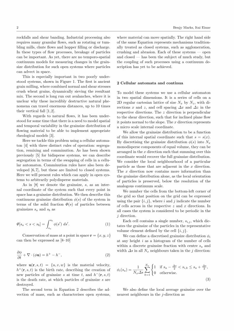
2 Benjy Marks, Itai Einav

rockfalls and shear banding. Industrial processing alsorequires many granular flows, such as rotating or tum-bling mills, chute flows and hopper filling or discharge.In these types of flow processes, breakage of particles

can be important. As yet, there are no temporo-spatialcontinuum models for measuring changes in the grain-size distribution for such open systems where particles

can advect in space.

This is especially important in two poorly under-stood systems, shown in Figure 1. The first is ancient

grain milling, where combined normal and shear stressescrush wheat grains, dynamically sieving the resultantmix. The second is long run out avalanches, where it isunclear why these incredibly destructive natural phe-

nomena can travel enormous distances, up to 10 timestheir vertical fall [1,2].

With regards to natural flows, it has been under-

stood for some time that there is a need to model spatialand temporal variability in the grainsize distribution offlowing material to be able to implement appropriate

rheological models [3].

Here we tackle this problem using a cellular automa-ton [4] with three distinct rules of operation: segrega-tion, remixing and comminution. As has been shown

previously [5] for bidisperse systems, we can describesegregation in terms of the swapping of cells in a cellu-lar automaton. Comminution rules have also been de-

veloped [6,7], but these are limited to closed systems.Here we will present rules which can apply in open sys-tems to arbitrarily polydisperse materials.

As in [8] we denote the grainsize, s, as an inter-nal coordinate of the system such that every point inspace has a grainsize distribution. We then describe thiscontinuous grainsize distribution φ(s) of the system in

terms of the solid fraction Φ(s) of particles betweengrainsizes sa and sb as

Φ[sa < s < sb] =

∫ sb

sa

φ(s′) ds′. (1)

Conservation of mass at a point in space r = {x, y, z}can then be expressed as [8–10]

∂φ

∂t+∇ · (φu) = h+ − h−, (2)

where u(r, s, t) = {u, v, w} is the material velocity,h+(r, s, t) is the birth rate, describing the creation of

new particles of grainsize s at time t, and h−(r, s, t)is the death rate, at which particles of grainsize s aredestroyed.

The second term in Equation 2 describes the ad-vection of mass, such as characterises open systems,

where material can move spatially. The right hand sideof the same Equation represents mechanisms tradition-ally treated as closed systems, such as agglomeration,crushing and abrasion. Each of these systems — open

and closed — has been the subject of much study, butthe coupling of such processes using a continuum de-scription has yet to be achieved.

2 Cellular automata and continua

To model these systems we use a cellular automatonin two spatial dimensions. It is a series of cells on a

2D regular cartesian lattice of size Nx by Nz, with di-rections x and z, and cell spacing ∆x and ∆z in therespective directions. The z direction is perpendicular

to the shear direction, such that for inclined plane flowit points normal to the slope. The x direction representsa micro scale internal coordinate.

We allow the grainsize distribution to be a function

of this internal spatial coordinate such that s = s(x).By discretising the grainsize distribution φ(s) into Nxmonodisperse components of equal volume, they can be

arranged in the x direction such that summing over thiscoordinate would recover the full grainsize distribution.We consider the local neighbourhood of a particularparticle as those that are adjacent in the x direction.

The x direction now contains more information thanthe grainsize distribution alone, as the local orientationof particles is preserved, below the resolution of the

analogous continuum scale.

We number the cells from the bottom-left corner ofthe grid so that position on the grid can be expressedusing the pair {i, j}, where i and j indicate the number

of cells across in the respective z and x directions. Inall cases the system is considered to be periodic in thej direction.

Each cell contains a single number, si,j , which dic-

tates the grainsize of the particles in the representativevolume element defined by the cell {i, j}.

We can define a discretised grainsize distribution φiat any height i as a histogram of the number of cells

within a discrete grainsize fraction with centre sa andwidth ∆s in all Nx neighbours taken in the j direction:

φi(sa) =1

Nx∆s

Nx∑

k=1

{1 if sa − ∆s

2 < si,k ≤ sa + ∆s2 ,

0 otherwise.

(3)

We also define the local average grainsize over thenearest neighbours in the j-direction as

The interactions between comminution, segregation and remixing in granular flows 3

Fig. 2 The cushioning effect and nearest neighbour rule. Left:

Large particles are cushioned such that they will not breakbecause of an abundance of small particles. Right: Small parti-cles do not carry a significant amount of load as they are freeto move in interstitial pore spaces. Top: Initial conditions.Bottom: Result after one iteration of the cellular automatarule, where on the left the small particles in a cell (orange)become even smaller (green), and on the right the large par-ticles in a cell (blue) become smaller.

si,j = (si,j−1 + si,j+1)/2, (4)

and similarly for the i-direction. For the cellular au-tomata rules defined below, we need to define two new

operators: sa ⇔ sb represents the swapping of valuessa and sb between their respective cells, and sa ⇒ sbrepresents a change in grainsize in the cell containing

sa to the new value of sb.

In the limit of infinitesimal cell size, the cellular au-tomaton may be regarded as a first order partial differ-ential solver [11]. In fact, there are many ways to recover

continuous results from such a cellular automaton [12].

3 Closed systems

We begin by considering closed systems, which are thosein which material does not advect in space such that

u = 0. There are many processes that have previouslybeen represented as closed systems, such as comminu-tion, agglomeration and abrasion. We here look only

at comminution, where particles are crushed to formfragments of smaller sizes.

Following the formulation in [10], for the case whereparticles are created only by the fragmentation of largerparticles, we can express the death rate as

h−(s, t) = b(s)φ(s, t), (5)

where b(s) is some specific breakage rate which governs

the frequency at which particles of grainsize s breakinto smaller fragments. The birth rate is then the sumof breakages into size s over all particles larger than s,

which can be expressed as

h+(s, t) =

∫ ∞

s

b(s′)P (s|s′)φ(s′, t) ds′, (6)

where P (s|s′) is a probability density function whichdictates the probability of creating grainsize s fromcrushing a particle of grainsize s′. We can then express

conservation of mass as

∂φ(s, t)

∂t=

∫ ∞

s

b(s′)P (s|s′)φ(s′, t) ds′ − b(s)φ(s, t). (7)

In a discrete sense, such as that defined in the cel-lular automaton, we can rewrite this equation as theconservation of a grainsize fraction with centre sa andwidth ∆s, over a time step ∆t as

∆φi(sa)

∆t=

Ns∑

k=a+∆s

(bi(sk)P (sa|sk)φi(sk)∆s

)−

bi(sa)φi(sa), (8)

where Ns is the total number of evenly spaced bins of

size ∆s. These equations have been considered manytimes before [13–16], and solutions have been proposedfor many mechanisms of comminution, such as grinding,cleavage and abrasion. However, breakage mechanisms

are normally assumed with a priori knowledge of powerlaw distributions [9,13]. In fact, in most models, eitherthe breakage rate b, the fragment probability distribu-

tion P , or both, are generally assumed to be power lawin nature from the outset [13].

Another method to model the problem has been

proposed in various forms, and uses simple geometricanalogies in a cellular automaton [6,7] where power lawpatterns are found, not imposed, by assuming that par-ticles with neighbours of the same size are likely candi-

dates to crush.

We can unify these two approaches, of macroscopicgrainsize distribution changes, and microscopic near-

est neighbourhood behaviour, by including the grain-size distribution in a cellular automaton.


αf = 1.71 αf = 1.94 αf = 2.26

αf = 1.99 αf = 1.99 αf = 2.23

10−510−410−310−210−1100Grainsize, s

10−510−410−310−210−1100

CG

SD,F

αf = 2.00 αf = 1.99 αf = 2.22

αi = −5

αi = −2

αi = 1

β = 0.05 β = 0.2 β = 0.8

Fig. 3 Evolving cumulative grainsize distributions due tocomminution. All simulations have Nz = 1, Nx = 106 andkb = 1. Three initial conditions are considered, with αi = –5,–2 and 1. Each initial condition is crushed at three values ofβ = 0.05, 0.2 and 0.8. Within each sub-plot, each line repre-sents a different time t = 0, 0.05, 1, 2 and 10, from bottomright to top left.

3.1 The crushing mechanism

When a large particle is surrounded by small particles,it is cushioned from fracture by having many points of

contact with neighbours, leading to a fairly isotropicloading state, as shown on the left of Figure 2. Also,when a small particle is surrounded by large particles,

it does not carry significant load, as it is either able tofit in the pore spaces if sufficiently small, or is highlymobile, as on the right of Figure 2. Because of this,we consider fracture of particles only when they are

surrounded by particles of a similar size. We then havea condition for fracture such that for a particle of sizesi,j and a local neighbourhood of particles of average

grainsize si,j ,

si,j ⇒ (0, 1)× si,j , if |si,j − si,j | ≤ βsi,j . (9)

This rule states that all particles in the representa-tive volume defined at si,j reduce in size by a randomly

chosen factor between 0 and 1 if it is within βsi,j ofthe local mean grainsize. The non-dimensional factor βdetermines how similar particles must be to their neigh-

bours before crushing can occur. We have also includeda factor of sj on the right hand side of the inequal-ity to make small particles harder to crush, recognising

that smaller particles have a higher crushing stress thanlarger ones [17]. This crushing event has some frequencywhich is proportional to the shear strain rate, allowingus to define the breakage rate as

bi,j = kb|γi|H (βsi,j − |si,j − si,j |) , (10)

10−8 10−7 10−6 10−5 10−4 10−3 10−2 10−1 100

Grainsize, s

10−5

100

CG

SD,F

αi=

−2.0

αi=

2.01

αf = 2.97

100 101 102 103 104 105 106 107 108 109 1010

Normalised grainsize, s/sm

10−30

10−15

100

N(∆

>s)

α = 2.07

αf = 3.00

Fig. 4 Cycles of breakage towards an attractor. Top: Cumu-lative grainsize distributions at different numbers of cyclesof loading. Each line represents the grading after a certainnumber of crushing-remixing cycles. From bottom right totop left, they are 0, 1, 10, 50, 100 and 500 cycles. The systemapproaches α = 3, or a horizontal line in this plot. Bottom:

The same data as in the top plot, now shown as number ofparticles ∆ greater than a certain size s. Insets show zoomedareas of original plot.

where kb is a non-dimensional fitting parameter and His the Heaviside function. In (9) we have also defined

the fragment size distribution as

P (sa|si,j) = ∆s/si,j , (11)

where ∆s is the size of the grainsize bin in the s di-

rection containing fragment size sa. The simulation oc-curs over Nx cells, spaced ∆x apart. Initial conditionsare generated by sampling Nx times from F = ∆x toF = 1 linearly along the inverse power law distributions

defined by

s = F 1/(3−αi). (12)

where F (s) =∫ ssmφ(s′) ds′ is the cumulative grainsize

distribution function and 3 − αi is the power law gra-dient. By time marching with a sufficiently small timestep, such that bi∆t ≤ 1, we implement the frequencyof breakage in a probabilistic manner.

Figure 3 shows three different initial conditions, andtheir progression to a steady state grainsize distribu-tion. Each initial condition is considered for three val-

ues of β. For each case, a new distribution is reachedafter a single timstep of ∆t = 0.05. As time progresses,β controls most of the behaviour of the process. For

small values of β, a steady state is reached where thegrainsize distribution does not change appreciably af-ter time t = 5, resulting in a power law dimension ofα = 1.99 ± 0.01. For large β, all of the largest parti-

cles are continually crushed, eventually resulting in asystem where α approaches 3.


104 105 106

L, Length of interrogation window

1.9

2.0

2.1

α

Fig. 5 Fractal dimension α against interrogation windowlength L. α value is measured as a best fit of the cumula-tive grainsize distribution from s = 10−4 to 10−1, restrictedto the cells between j = a±L/2. Each line represents a differ-ent value of a = 0, Nx/4, Nx/2 and 3Nx/4. For this simulationNx = 106, β = 0.2, kb = 1 and αi = −2.

The cellular automata predicts the same final grain-

size distribution largely independent of the initial grad-ing, with some minor effects due to the initial concen-tration of very large particles. Such a power law grad-

ing of the grainsize distribution has been measured inother cellular automata [6,7], discrete element simula-tions [18] and experiment [2].

Generally fractal dimensions are measured in fault

gauges, confined comminution tests and rock avalanchesin the range of α = 2 – 3 [19–21]. The limiting valueof α = 2 for most cases of our model can be explained

using the cellular automaton developed in [20], whereevery particle in the systems has the same probability ofcrushing, given some additional geometric constraints.If this probability is exactly 0.5, the system develops

a fractal dimension of α = 2. If the probability is 1,the system reaches α = 3, which represents a systemwith large strain, where nearest neighbours change over

the crushing period [22]. This distribution in fact cor-responds to a random appollonian packing, as in [23].

In Figure 5 α is measured many times in a single

simulation. A number of cells, L, centred at a, are cho-sen, and a best fit of α is measured for the cumulativegrainsize distribution. With increasing zoom into thesystem, the measured power law does not change slope

significantly. This is an indication of a fractal distribu-tion [6].

The idea of such final power law grainsize distribu-

tions has been applied in [24] to develop a thermody-namically consistent theory for comminution processesin granular materials in closed systems. Extension of

this or other theories to open systems where particlescan advect has not yet been achieved.

Time, t

Hei

ght,z

Fig. 6 Bidisperse cellular automaton. Top: Schematic repre-senting bidisperse segregation in 2D flow down an inclinedplane. Bottom: The complimentary 1D cellular automaton,where large particles and small particles swap over time.

3.2 Comparison with continua

To compare the cellular automata rules with a contin-uum, we consider the evolution of a large number of

cells simultaneously, and find averaged properties thatrepresent the continuum scale. We express the breakagerate, bi, of a single grainsize fraction sa covering sizes

over a range of ∆s as

bi =kb|γi|Nx

Nx∑

j=1

H (βsi,j − |si,j − si,j |) . (13)

To solve this system globally, we need to sum over

j, which represents local information about the nearestneighbours. If we were to represent this in a continuumsense, this local information is smaller than the contin-

uum scale, and so a new length scale, ζ, must be intro-duced. In the cellular automaton, the length scale whichcontrols this behaviour is that of the nearest neighbour

zone (here set arbitrarily to ∆x). By increasing the sizeof the neighbourhood over which we find the local av-erage grainsize, the system would converge towards adifferent state, where physical proximity of neighbours

is not considered.

How to introduce such a length scale in a continuumtheory is an open question. In the cellular automaton,

we can consider changing this length scale by doingcycles of crushing, as will be shown below.


sm sMGrainsize, s

−1

0

1

f/(k

sγ)

0 s 2s

Grainsize, s

−1

0

1

f/(k

sγ)

Fig. 7 The segregation mechanism as a function of gransize s.Left: Bidisperse rule used previously in [5] Right: Polydisperserule used here, where segregation frequency is a function ofdistance to the local mean size.

3.3 Cycles of crushing: Towards open systems

We can extend this simulation to a quasi-open systemby considering a rearrangement of particles within thecellular automaton, but without true advection.

After the system has reached steady state, and nofurther significant crushing will occur, we shuffle thesystem, relocating all of the nearest neighbours, and

resume crushing until a new steady state is reached. Wecan continue this cycle until an ultimate steady state isreached.

We begin with the simulation shown in the centre ofFigure 3, which has an initial grading defined by αi =−2, and after one full crushing iteration process has

reached α = 2. As progressively more iterations occur,a region of higher slope develops at larger grainsizes,and this propagates to lower grainsizes with increasingiterations, as shown at the top of Figure 4. This trend is

towards α = 3, however this coincides with a horizontalline in this plot, and cannot be seen clearly. To visualisethis more clearly, the bottom plot in Figure 4 shows the

same data, but plotted as the number of particles ∆greater than a certain size s, such that the slope of thegraph is α. We define the number of particles per cell as

being inversely proportional to the size cubed. The finalstate has been shuffled and crushed 500 times, tendingtowards an ultimate grading with this new power lawgradient of αf = 3.

This effect of cycles of crushing towards αf = 3 hasbeen observed experimentally [25], numerically with acrushable discrete element method [26] and predicted

analytically as the maximum entropy path towards theleast efficient packing of the system [23]. It is remark-able that such a simple, one dimensional system as this

can replicate the packing involved in such a complexsystem.

4 Open systems

In order to model open systems, where particles canadvect between points in space, we need rules for ad-

0 4Time, t

0

1

Hei

ght,z

0.5

1.0

s

Fig. 8 The time evolution the average grainsize s of a bidis-perse simulation with varying Nx subject to segregation only.All cases have ks = 1 and Nz = 100. Clockwise from Top Left:

Nx = 1, 10, 100 and 1000. For the case of Nx = 1 we find thelocal average grainsize in the z direction. Bottom right: Blacklines indicate positions of concentration shocks from solutionof analogous continuum equation.

vection. To be a truly physical model, we need to satisfythe conservation equation for grainsize φ such that

∂φ

∂t+∇ · (φu) = 0. (14)

We set up our rules for the cellular automaton suchthat this conservation law is held for some velocity u.

The first mechanism we consider is due to segregation.Towards this end, we begin with the simplest case ofsegregation and describe bimixtures, where we present

a model similar to that proposed in [5].

4.1 The segregation mechanism

As particles flow they collide, creating new void spaceswhich are preferentially filled by smaller particles mov-ing, as in Figure 6. The rate of creation of void spaces

is governed by the shear strain rate, γ.

The simplest description of this system in terms ofgrainsize is shown on the left of Figure 7 for a bimixture

of sizes sm and sM , where the swapping frequency f isdefined such that small particles always move down,and large particles move up.

We can extend this model to describe polydispersematerials by using the formulation developed in [8],where it was shown through energy considerations thatif a particle is larger than the local average, it has some

probability of moving up, and conversely if it is smallerthan the average it will move down. Increasing distancein the s direction from the average will increase the like-

lihood of swapping linearly. This is shown on the rightof Figure 7.


0 5Time, t

0

1

Hei

ght,z

sm

sM

s

Fig. 9 Time evolution for bidisperse shear flows subject tosegregation. For all cases ks = 1. Left to right: The systemis initially filled with 20%, 50% and 80% small particles re-spectively. Top row: Simple shear, where γ = 1. Bottom row:Inclined plane flow shear condition, where γ =

√1− z.

We facilitate this movement by swapping this grain-size with that either above, si+1,j or below, si−1,j de-

pending on whether it is smaller or larger than theaverage size si,j . We define the rate of swapping asf = ks|γi|(si,j/si,j − 1), with the sign determining the

direction:

if

{f > 0, si,j ⇔ si+1,j

f < 0, si,j ⇔ si−1,j .

where ks is a non-dimensional parameter controlling therate of segregation. We iterate in two half time steps,alternately applying this rule firstly to all odd rows,

and then all even rows, so that particles are inhibitedfrom moving very large distances in a single time step.Additionally, we only allow swapping upwards if the

particle is larger than the one above it, or smaller thanthe one below it if moving downwards.

4.2 Bidisperse segregation

To model a simple bidisperse material, we take a singlecolumn of a bimixture (Nx = 1), of equal proportions of

sizes sm and sM , randomly allocated to cells, and allowit to segregate under simple shear with γ(z) = 1 andks = 1. The result is shown in the top left of Figure

8. We can then run the simulation with Nx = 5 andaverage over the x-direction. The result of this is shownin the top right of Figure 8. We can do this repeatedly,to get an increasingly resolved image of the process, as

shown in the bottom row of Figure 8 for Nx = 50 and1000. With increasing resolution, this converges on theanalytic solution presented in [8] and [27].

Figure 9 shows the average grainsize at each heightover time for two different shear regimes, each for 3 dif-ferent initial concentrations of small particles, sm. The

top row depicts simple shear, as in Figure 8, while thebottom row uses a simplified version of the shear strain

10−1 100Grainsize, s10−3

100

CG

SD,F

0 5Time, t0

1

Hei

ght,z

10−1 100Grainsize, s0

1

CG

SD,F

10−1

100

s

Fig. 10 Polydisperse segregation under simple shear. For allcases ks = 1 and γ = 1. Top to Bottom: Each row represents asingle simulation with initial condition defined by αi = −2, 0and 2 respectively. Left: Initial cumulative grainsize distribu-tion at three different heights. The solid red, dashed green anddash-dotted black lines represents z = 0.9, 0.5 and 0.1 respec-tively. Middle: Plot of the average grainsize s over height andtime. Right : Final cumulative grainsize distributions, plottedin the same manner as the initial grainsize distributions.

rate profile predicted in [8] for the case of inclined planeflow: γ =

√(1− z)/s. In each case, complete segrega-

tion is observed, where every large particle lies above

every small particle. The non-uniform shear strain ratein the bottom case causes non-uniform transient be-haviour towards a steady grading that is the same as

the top case. According to the formulation presentedhere, the final grading is independent of the loadingcondition.

As shown in [5], this model represents a very simpleanalogy of the analytic works done by [28,27] to model

bidisperse segregation, with a very simple extension topolydisperse systems, as shown below.

4.3 Polydisperse segregation

We can create a polydisperse sample by generating ini-tial conditions in the same way as previously describedfor the breakage cellular automaton, using Equation 12.

The segregation patterns produced for a range of ini-tial conditions at constant segregation rate ks = 1 andwith γ = 1 are shown in Figure 10. Since this is now a

polydisperse sample, we can calculate the grainsize dis-tribution φ(s). On the left hand side of Figure 10 are theinitial cumulative grainsize distributions, which are ho-mogeneous. During the simulation, segregation occurs,

creating a non-homogeneous steady state condition af-ter some time. These grainsize distributions, which nowvary with height, are shown on the right hand side of

the same Figure.

Averaging over all cells at a given height i, we canexpress the mean segregative velocity ui of a single


Time, t

Hei

ght,z

Fig. 11 The mixing mechanism. Ten cells, initially segre-gated with all large particles (blue) above small particles (yel-low), subjected to the mixing mechanism only. Over time, thesystem reaches a disordered state.

grainsize fraction centred at sa from all cells at heighti in a time ∆t as

ui(sa) =1

Nx

Nx∑

j=1

fi,j(sa) =ks|γi|Nx

Nx∑

j=1

(sasi,j− 1

). (15)

We have included the local average grainsize si,j inthe formulation so that we know which particles arelocally small or large. As particles are being swappedbetween heights — between representative volume ele-

ments at the continuum scale — we only require a singleaverage grainsize per height, and can in this case freelyextend the neighbourhood domain over which we find

the average grainsize s to include every cell at heightj, labelling it now si = 1/Nx

∑j si,j . In this case, the

mean velocity can be expressed as

ui(sa) = ks|γi|(sasi− 1

). (16)

Compare this with the analytic description of the

segregation velocity with no diffusion as predicted by[8] for a continuum with internal grainsize coordinates,

u(s) = |γ|g cos θ

c

(ss− 1), (17)

where c is a fitting parameter, g is the acceleration dueto gravity, and θ is the angle of the plane down which

flow is occurring. As shown in [29], cellular automatacan successfully be used as a coarse finite differencingmethod to model systems such as these without resort-

ing to complicated flux limited finite difference schemes,as would otherwise be necessary.

0 10Time, t

0

1

Hei

ght,z

0.5

0.6

0.7

0.8

0.9

1.0

s

Fig. 12 The time evolution the average grainsize s of a bidis-perse simulation with varying Nx subject to mixing only. Allcases have D = 0.01 and Nz = 100. Clockwise from Top Left:Nx = 1, 5, 50 and 1000. Bottom right: Solid lines indicatecontours from solution of analogous continuum equation.

This model, together with the rule for remixing,

which will be shown next, represents the simplest de-scription of the analytic description presented in [8].

4.4 Remixing

In nature we rarely see such perfect segregation as thatpictured above. This is due to the random fluctuation ofparticles as the flow propagates down slope. As has been

done before analytically [30], we can capture this effectby introducing remixing into the flow. For the simplestcase, we allow particles to swap randomly either up ordown with some frequency, given by a constant D/∆z2.

At this stage we let this probability be independent ofthe shear strain rate γ, although a strong dependencyhas been observed [31] in experiments. With frequency

of swapping controlled by the diffusivity, D,

Flip a coin, if heads: si ⇔ si−1

if tails: si ⇔ si+1

An example of the mixing rule acting on a singlecolumn of cells over time is shown in Figure 11. Ini-tially, the system is perfectly segregated, but over time

the systems becomes randomised due to the presence ofremixing. The characteristic time for mixing to occur isthe inverse of the diffusivity D/H2.

We are describing a system of cells undergoing Brow-nian motion, whereby particles move by the applicationof random forces over time scales that are short rela-tive to the motion of the particle. When considered over

long time scales and large numbers of particles, this isanalogous to Fickean diffusion [31]. Many other cellularautomata exist to model pure diffusion [32].

As in the case of segregation, this process can beaveraged over the x direction to describe the evolution


Fig. 13 Coupled comminution and mixing. Varying valuesof D/(kbH2). For all cases, Nz = 21, Nx = 1000. Plot showsfinal value of best fit to power law part of cumulative grainsizedistribution at t = 5, 50 and 500, corresponding to the solid,dashed and dash-dotted lines respectively.

of the average grainsize at any height over time. Byincreasing the number of cells in the x direction, we

can increase the smoothness of our solution. Figure 12shows the same system as Figure 11, initially segre-gated, that mixes over time to create a homogeneoussystem, but now for increasing numbers of cells in the

x direction.This diffusive behaviour can be described at the con-

tinuous limit using Fick’s first law of diffusion,

∂φ

∂t= D

∂2φ

∂t2. (18)

5 Coupled problems

We now have three distinct processes which can be de-scribed simultaneously in a single simulation. These

have all been shown above with their analogous con-tinuum description, yet not in all cases could a directlink be shown. For the case of comminution, an internallength scale governing the spatial distribution of grain-

size over a sub-continuum length scale was required.As all of the mechanisms previously described have

been created in the same framework, we can simply run

a cellular automaton which includes multiple phenom-ena at the same time. As will be shown in this Section,we can investigate the interactions between the mech-

anisms by varying the parameters which control theireffects.

5.1 Comminution and mixing

We begin with a cellular automata that includes bothcomminution and mixing. This system represents an ex-

Fig. 14 Bidisperse segregation under simple shear with diffu-sion. Left to Right : Increasing diffusivity D = 0.002, 0.01 and0.05 with constant segregation coefficient ks = 1. Increasingthe mixing coefficient smooths out concentration shocks inthe spatial direction, giving more physically representativesolutions.

tension of the cycles of crushing pictured in Figure 4,

but now with true advection. In this case, as in Figure4, we expect that after a short time relative to the dif-fusive time, the system will reach αf = 2, as significant

mixing has not yet occurred. At longer times, the sys-tem will approach αf = 3, and its final grading. Thiseffect is captured in Figure 13, where the diffusive time

is controlled by the ratio D/(kbH2), and the system is

constrained at αf = 2.91.

For vanishingly small diffusivities, the system willstill approach αf = 3, but only after very long periods

of comminution. Conversely, at very large diffusivities,the system passes αf = 2 very rapidly, and approachesαf = 3 in a relatively short time.

5.2 Segregation and mixing

In flows of polydisperse granular materials where com-minution does not occur, we can model the evolution of

the grainsize distribution as being comprised of segrega-tive and diffusive remixing components. This occurs inmany industrial mixing processes, and may be sufficientto model levee formation and runout characteristics in

landslides. At higher speeds remixing increases, sup-pressing segregation, while at low speeds segregationcan play a dominant role in the flow behaviour.

The effect of coupling mixing and segregation in a

bimixture can be seen in Figure 14, where increasingdiffusivity D smooths out the concentration shock be-tween the two phases of large and small particles. This

can be treated in an identical manner for polydispersemixtures.

This has been shown analytically for bidisperse sys-tems in [30] and validated experimentally in [33].

Generally, suppressing spurious numerical diffusion

is a non-trivial task, requiring sophisticated finite dif-ferencing schemes [34] to maintain hyperbolicity. Thistype of stability, which generally controls the accuracy

of the numerical results, is not an issue for solutionsobtained using cellular automata [5].


Fig. 15 A crushable flow with two mechanisms: segregation and comminution. Initially, the system is homogeneous, being apolydisperse sample with initial grainsize distribution defined by αi = −2. Four cases are considered with varying kb and ks.For each case, three plots are shown. Top: Evolution of the average grainsize at every height over time. Bottom left: Cumulativegrainsize distribution at three points in the flow, corresponding to the crosses in the above plot. Top is red solid line, middleis green dashed line and bottom is black dash-dotted line. Bottom right: Cumulative grainsize distributions at steady state atsame heights as previously. Solid blue lines represent best fit cumulative log-normal distributions.

5.3 Segregation and comminution

In many situations, segregation and comminution oc-cur simultaneously in a flow situation, such as in thegrain milling depicted in Figure 1. In other cases, it

is not even clear if segregation has occurred, yet par-ticles are advecting in space and strong comminutionis observed, such as in earthquake faulting and snowavalanches. In many of these cases, we observe log-

normal grainsize distributions, rather than power lawdistributions, which exist at all depths of flow. The ex-istence of these curves represents the competition be-

tween the two mechanisms, where the comminution at-tempts to form a power law distribution, and the seg-regation attempts to create a locally monodisperse dis-

tribtion. A log-normal distribution is one that obeysthe following scaling for the cumulative grainsize dis-tribution FLN ,

FLN =1

2erfc

(− ln s− µ

σ√

2

), (19)

where µ and σ are the location and scale parameters,and erfc is the complimentary error function.

In Figure 15, simulations are shown in which bothsegregation and comminution are present. For all cases,

log-normal cumulative grainsize distributions are ob-served over all depths, with p-values in the bottom halfgenerally less than 0.001.

As expected, increasing ks or kb decreases the time

to reach a steady state in terms of the average grainsizes. It is evident that significant changes in the grainsizedistribution will not occur indefinitely, even though seg-

regation brings together particles of similar size, andcomminution is accelerated by the segregation.

5.4 Segregation, mixing and crushing

We can now couple all three mechanisms and observethe evolution of the grainsize distribution as all of theconstituent mechanisms interact. Each time step, we

first check each cell and if the breakage rule is met,we change the cell’s grainsize. Secondly, we iterate over


0 25Time, t

0

1

z

10−5 1Grainsize, s

0

1

CG

SD,F

10−2

10−1

100

s

Fig. 16 A crushable flow with all three mechanisms. For allcases ks = kb = 1 and H = 1 is the height of the system.Initially, the system is homogeneous, being a polydispersesample with initial grainsize distribution defined by αi = −2.Each row represents the same initial condition but with vary-ing amounts of mixing. From top to bottom, D = 0, 0.005and 0.05 respectively. Left: Cumulative grainsize distributionaveraged at three heights z = 0.1, 0.5 and 0.9 at steady state(black, green and red respectively). Right: The average grain-size at every height evolving over time.

all of the cells and swap them with a neighbour if thesegregation rule is met. Finally, we again iterate over allcells and if the diffusion rule is met, we swap randomly

with a neighbour.

We now have a system that models avalanche andlandslide flow, where particles at the base are shearedand crush, creating a lubrication layer, such as in Fig-

ure 15. The inclusion of mixing in the system, as shownin Figure 16, enhances the spread of sizes produced bycomminution, and reduces the size of particles in the

bottom-most layer of flow, enhancing the lubricationeffect. Again, log-normal cumulative grainsize distri-butions are measured, which represent those found inmany geophysical processes, such as in snow avalanches

[35].

5.5 An equivalent continuum model

Considering conservation of mass alone, we can expressall three mechanisms in a continuum form as

∂φ

∂t+ ks

∂

∂z

(φ|γ|

(ss− 1))

= D∂2φ

∂t2

+bφ−∫ sM

s

P (s|s′)b(s′)φ(s′) ds′. (20)

This model differs from the cellular automata in thesense that the internal coordinate s does not retaininformation about local neighbours. Because of this,

cycles of crushing cannot be produced. This omissiongives an important insight into the use of continuum

theories to represent internally (i.e. within the repre-sentative volume element) spatially correlated material.

For the mechanisms of segregation and mixing, thelength scale representing the local neighbourhood is notan important consideration. However for comminution,it must be included as part of the model to enable us

to predict the correct final distribution.

6 Conclusions

We have shown that cellular automata can successfullycapture the most important physical foundations be-

hind evolving phenomena in crushable granular flows.To do this, we have used three distinct cellular au-tomata to explain the dominant mechanisms during

such flows: comminution, segregation and mixing.

By assembling all three cellular automata together

we were able to explore the interactions between thesephenomena. One surprising outcome is that in closedsystems, crushable granular material are limited by power

laws, however during flow the interaction with segrega-tion and remixing the system is limited by log-normaldistributions.

This paper highlights the power of the cellular au-tomata as a means to inspire continuum models. Wehave demonstrated that it is often possible to recover

an analogous continuum description from the limit ofthe cellular automata rules. An interesting result of thistactic is the result that comminution does not follow

this rule. For comminution, the ability to model cyclesof crushing using a conventional continuum model witha grainsize coordinate is currently impossible, as some

local rules are inherent to the system that must be in-cluded to describe the local configuration of grains.

The success of this cellular automata is that it en-ables us to study the evolution and limits of the grain-size distribution in different scenarios. Current contin-uum models require a priori knowledge the grainsize

distribution, and cannot educate us on the physicalmechanisms involved in reaching this final state.

IE acknowledges grant DP0986876 from the ARC.

References

1. F. Legros, Engineering Geology 63, 301 (2002)2. B. Imre, J. Laue, S. Springman, Granular Matter 12(3),

267 (2010)3. R. Iverson, in Debris flow Mechanics and Mitigation Con-

ference, Mills Press, Davos (2003), pp. 303–3144. S. Wolfram, Advanced Series on Complex Systems, Sin-

gapore: World Scientific Publication (1986)5. B. Marks, I. Einav, Granular Matter 13, 211 (2011)6. S. Steacy, C. Sammis, Nature 353(6341), 250 (1991)


7. G. McDowell, M. Bolton, D. Robertson, Journal of theMechanics and Physics of Solids 44(12), 2079 (1996)

8. B. Marks, P. Rognon, I. Einav, Journal of Fluid Mechan-ics 690, 499 (2012)

9. S. Redner, Statistical models for the fracture of disor-dered media, New York: North-Holland 321, 348 (1990)

10. D. Ramkrishna, Population balances: Theory and applica-

tions to particulate systems in engineering (Academic PressSan Diego, 2000)

11. T. Toffoli, Physica D: Nonlinear Phenomena 10(1-2), 117(1984)

12. S. Rafler, ArXiv e-prints (2011)13. A. Randolph, R. Ranjan, International Journal of Min-

eral Processing 4(2), 99 (1977)14. T. Peterson, M. Scotto, A. Sarofim, Powder technology

45(1), 87 (1985)15. E.D. McGrady, R.M. Ziff, Phys. Rev. Lett. 58, 892 (1987)16. M. Williams, Aerosol Science and Technology 12(3), 538

(1990)17. W. Weibull, et al., Journal of applied mechanics 18(3),

293 (1951)18. O. Ben-Nun, I. Einav, A. Tordesillas, Phys.

Rev. Lett. 104(10), 108001 (2010). DOI10.1103/PhysRevLett.104.108001

19. Y. Ben-Zion, C.G. Sammis, Pure and Applied Geophysics160, 677 (2003)

20. D. Turcotte, Journal of Geophysical Research 91(B2),1921 (1986)

21. G.B. Crosta, P. Frattini, N. Fusi, Journal of GeophysicalResearch: Earth Surface 112(F1) (2007)

22. C. Sammis, G. King, Geophysical Research Letters 34(4),L04312 (2007)

23. G. Delaney, S. Hutzler, T. Aste, Physical review letters101(12), 120602 (2008)

24. I. Einav, Journal of the Mechanics and Physics of Solids55(6), 1274 (2007)

25. J. Lorincz, E. Imre, M. Galos, Q. Trang, K. Rajkai, S. Fi-tyus, G. Telekes, International Journal of Geomechanics5(4), 311 (2005)

26. B. Oded, Confined comminution of granular materials:Self-organisation, attractors and patterns. Ph.D. thesis,University of Sydney (2010)

27. J. Gray, A. Thornton, Proc. Roy. Soc. A 461(2057), 1447(2005)

28. S. Savage, C. Lun, Journal of Fluid Mechanics 189, 311(1988)

29. B. Marks, I. Einav, P. Rognon, in Advances in Bifurcation

and Degradation in Geomaterials, Springer Series in Ge-omechanics and Geoengineering, vol. 11, ed. by S. Bonelli,C. Dascalu, F. Nicot (Springer Netherlands, 2011), pp.145–151

30. J. Gray, V.A. Chugunov, Journal of Fluid Mechanics 569,365 (2006)

31. B. Utter, R.P. Behringer, Phys. Rev. E 69(3), 031308(2004). DOI 10.1103/PhysRevE.69.031308

32. B. Chopard, M. Droz, Journal of statistical physics 64(3-4), 859 (1991)

33. S. Wiederseiner, N. Andreini, G. Epely-Chauvin,G. Moser, M. Monnereau, J.M.N.T. Gray, C. Ancey,Physics of Fluids 23(1), 013301 (2011)

34. A. Kurganov, E. Tadmor, Journal of ComputationalPhysics 160(1), 241 (2000)

35. P. Bartelt, B.W. McArdell, Journal of Glaciology55(193), 829 (2009)

CHAPTER 9

Conclusion

This work has introduced the concept of the grainsize distribution into the modelling of gran-

ular flows. By including this additional internal coordinate, I have explained the mechanism

of segregation in the simplest possible way: a stress gradient in the grainsize direction. Also,

crushing during flow can be expressed in this framework in a simple manner, where both

fractal and power-law grainsize distributions evolve naturally.

In Chapter 3, beginning with the simple idea that segregation in one dimension can be

described as the swapping of particles, I have devised a cellular automata which is a repres-

entation of the basic physics required to describe kinetic sieving for steady flows.

In this model, I have shown that the previous analytic work on kinetic sieving can be con-

solidated into a cohesive, concise theory which contains the essence of both works. This

simplistic model of segregation can reproduce the behaviour observed in both continuum

mechanics and statistical mechanics representations of the same phenomenon. The cellular

automaton, however, gives no insight as to what is causing the segregation during granular

flows. Finally, this paper shows how cellular automata can be used as an alternative means to

solve hyperbolic partial differential equations with concentration shocks, as they suffer from

fewer numerical instabilities.

In Chapter 4, I have derived the first polydisperse theory for granular segregation by introdu-

cing the grainsize coordinate. The resulting five dimensional continuum theory explains the

mechanism of kinetic sieving as a stress gradient in the grainsize direction, and captures the

interplay between segregation and remixing.

95

96 9 CONCLUSION

By including a simple constitutive model that scales with the mean local grainsize, the

kinematics can be directly related to the grainsize dynamics, allowing us to measure a

lubrication effect that is caused by segregation, which accelerates the flow. This model

predicts not only the grainsize distribution at every point in space and time within the flow,

but also the kinematics. I have successfully compared this theory with discrete element

simulations, and have shown that the theory can be used to model systems with arbitrary

grainsize distributions.

When the theory was used to represent a bimixture, comparison with previous theories was

possible. For this system, the role of size contrast between the two constituents was made

clear for the first time. For multi-component systems, it was shown that the only previous

theory was sensitive to how the sizes were binned, and as a result needed a large number of

fitting parameters that varied with time.

For one dimensional steady flows, such as many industrial flows, and geophysical flows on

smooth terrain, it is now possible to predict the time for segregation. Using this knowledge,

we can tailor conditions to either reduce or increase the extent of segregation as necessary.

The theory also predicted that small particles aggregating at the base of the flow can create a

lubrication effect.

A fluctuation decomposition of the continuum theory was shown in Chapter 5 that decouples

the bulk and grainsize dynamics. This validates the current theories of segregation, where

the segregation kinematics are dissociated from the bulk flow. Additionally, the explicit

description of the two systems using a grainsize-enhanced continuum theory allows for

implementation into existing numerical methods for large deformation flow problems.

The potential uses for such a tool are innumerable. This type of analysis could be used for

modelling in a large number of diverse fields of interest, such as tumbling mills, chute flows,

hopper discharge and filling, landslides, river sedimentation, off-world mining and planetary

ring dynamics.

In Chapter 6, a steady state solution of the continuum theory was developed. In many

situations, the time for segregation is much shorter than the time of flow, and so the time

9 CONCLUSION 97

dependent behaviour of the segregation is unimportant. In these cases, there is no reason to

solve the temporal problem, and a simpler set of ordinary differential equations was presented

that can be solved once the stress gradients and diffusivity of the system are known.

This solution highlights the fact that for systems with stable, steady state flows and arbitrary

grainsize distributions, segregation can be predicted. This is the first predictive model for

segregation patterns.

I have shown in an inclined chute experiment that the peak forces measured on impact

with a rigid obstacle depend strongly on the grainsize distribution of the incoming flow. At

approximately 5% fine particles a bidisperse avalanche of this sand reaches the largest peak

force, at the scale of the experiment 20% larger than if modelling with a monodisperse sand.

For the safe design of protection structures, this effect must be quantified and considered, as

monodisperse tests will give non-conservative estimates of the design loads on a structure.

The prediction of this force has not been considered in this work, but can be posed in terms of

the spatial variability of the grainsize distribution in a 2D or 3D flow geometry. To do this,

the theory described in Chapter 5 needs to capture the changes in the grainsize distribution

during flow, and to use constitutive laws that depend on the local grainsize distributions. In

this way internal rheology, basal roughness effects, and wall interaction can all be expressed

in terms of their dependence on the grainsize distribution. It is only when we have this level

of understanding of the kinematics of flowing granular material that will we be able to safely

design protection structures to impede the flow of avalanches, debris flows and landslides.

Finally, expanded cellular automata were derived to describe polydisperse segregation, mixing

and comminution in Chapter 8. The segregation and mixing automata were shown to represent

analytic solutions that have already been validated experimentally and numerically. The

comminution automaton was shown to predict power law distributions in no flow conditions,

which represent physical solutions as measured in experiment and numerical analysis. By

coupling these automata together, I have shown how the interaction between these mechanisms

gives rise to stable log-normal grainsize distributions which are depth dependent, as measured

98 9 CONCLUSION

in landslides, debris flows and avalanches. This is the first predictive model of log-normal

grainsize distribution evolution.

I have also shown how the cellular automata described in Chapter 8 can be used to inspire

continuum models, and how the grainsize coordinate can be used to describe population

balance models that do not require a priori knowledge of the final grading curves.

Together, this body of knowledge allows us, for the first time, to see the utility of including a

grainsize coordinate in a numerical or analytic description of a granular system. By adding this

ingredient, complex phenomena can be described simply and accurately. This is a paradigm

shift in the description of granular materials for the fields of research that study granular

flows, such as glaciology, snow avalanches, debris flows, landslides, erosion processes, hopper

filling and discharge, comminution and draw down mining.

By expanding on the work undertaken during my PhD, we will see significant improvement

in the understanding, modelling, efficiency, and safety of these industries.

9.1 Future outlook

Clearly, there is much work to do be done to push this work further. The first step of this

process would be to incorporate the fluctuation decomposition shown in Chapter 5 into a two

or three dimensional model, so that investigations of segregation in other geometries can begin

systematically. This would allow for an understanding of levee formation during avalanche

runout and segregation induced mobility changes. In addition, the fluctuation decomposition

should be extended to include crushing.

I believe that a material point method implementation either with or without crushing would

allow us to realise these goals. Once crushing is included, we can look at draw down mining,

snow avalanches, and the effect of crushing in large mobility avalanches. Also, there would be

large applicability to the design of mixers and crushers for the mining and chemical processing

industries.

9.1 FUTURE OUTLOOK 99

A further refinement to the theory would be the inclusion of a passive fluid phase, as described

for a bimixture in Thornton et al. (2006). The role of spatial variability of pore pressures

during debris flow could then be studied, as these appear to control the granular fronts and

liquid tails observed in nature. Once that is complete, the work would benefit from a full

decoupling into a two phase material of separate fluid and granular fluid components so that

erosion and deposition could be modelled.

An assumption made in Chapter 4 was that the diffusivity, D was independent of grainsize.

From preliminary discrete element investigation, it appears that this is not the case. It would

behove us, then, to find a scaling law to represent the true variability of diffusion with

grainsize.

A further assumption in Chapter 4 was that the inertial time scaled with the mean particle size.

This has not been validated experimentally. Large deformation shear tests, such as in a ring

shear or stadium shear device, would be able find the relationship between viscosity and the

grainsize distribution.

Finally, experimental validation of the ideas presented in this dissertation are lacking. To

validate these theories, full field measurements of three dimensional flows are required from

experimental and numerical analyses. While these tools are being developed I would urge

those interested to find an existing experimental apparatus, and re-run previous tests but now

varying the grainsize distribution. With a good collection of boundary value measurements

for a variety of flow problems, we can expand our understand of the grainsize dynamics in

granular flows.

Bibliography

ABS-Lawinenairbags, Peter Aschauer GmbH (Apr. 2013). Operating Principle. URL: http:

//abs-airbag.de/en/abs-system/stay-on-top-to-stay-alive/.

Alonso, JJ and HJ Herrmann (1996). ‘Shape of the tail of a two-dimensional sandpile’. In:

Physical Review Letters 76.26, pp. 4911–4914.

Alonso-Marroquin, Fernando and Yucang Wang (2009). ‘An efficient algorithm for granular

dynamics simulations with complex-shaped objects’. In: Granular Matter 11.5, pp. 317–

329.

Andò, Edward et al. (2012). ‘Grain-scale experimental investigation of localised deformation

in sand: a discrete particle tracking approach’. In: Acta Geotechnica 7.1, pp. 1–13.

Armanini, Aronne (2013). ‘Granular flows driven by gravity’. In: Journal of Hydraulic

Research 51.2, pp. 111–120.

Arya, Lalit M and Jack F Paris (1981). ‘A physicoempirical model to predict the soil moisture

characteristic from particle-size distribution and bulk density data’. In: Soil Science Society

of America Journal 45.6, pp. 1023–1030.

D2487, ASTM Standard (2011). Standard Practice for Classification of Soils for Engineering

Purposes (Unified Soil Classification System). ASTM International, West Conshohocken,

PA.

Bagnold, Ralph A. (1941). The Physics Of Blown Sand And Desert Dunes. Dover Earth

Science Series. Dover Publications.

Bagnold, Ralph A (1954). ‘Experiments on a gravity-free dispersion of large solid spheres in

a Newtonian fluid under shear’. In: Proceedings of the Royal Society of London. Series A.

Mathematical and Physical Sciences 225.1160, pp. 49–63.

Bagnoli, Frank (1941). Dynamical Modeling In Biotechnology. World Scientific. Chap. Cellu-

lar Automata.

100

http://abs-airbag.de/en/abs-system/stay-on-top-to-stay-alive/

http://abs-airbag.de/en/abs-system/stay-on-top-to-stay-alive/

BIBLIOGRAPHY 101

Bartelt, P and BW McArdell (2009). ‘Granulometric investigations of snow avalanches’. In:

Journal of Glaciology 55.193, pp. 829–833.

Bear, Jacob (1972). Dynamics of fluids in porous media. Courier Dover Publications.

Ben-Nun, O., I. Einav and A. Tordesillas (Mar. 2010). ‘Force Attractor in Confined Commin-

ution of Granular Materials’. In: Physical Review Letters 104.10, p. 108001.

Ben-Zion, Y. and C. G. Sammis (2003). ‘Characterization of Fault Zones’. In: Pure and

Applied Geophysics 160 (3-4), pp. 677–715.

Bertrand, F., L.-A. Leclaire and G. Levecque (2005). ‘DEM-based models for the mixing of

granular materials’. In: Chemical Engineering Science 60.8–9, pp. 2517 –2531.

Bingham, Eugene Cook (1917). An investigation of the laws of plastic flow. Vol. 13. 2. Govt.

Print. Off.

Boer, Gerben BJ de et al. (1987). ‘Laser diffraction spectrometry: Fraunhofer diffraction

versus Mie scattering’. In: Particle & Particle Systems Characterization 4.1-4, pp. 14–19.

Bolton, Malcolm D (2000). The role of micro-mechanics in soil mechanics. Tech. rep. Cam-

bridge University Engineering Department.

Bond, Fred C (1952). ‘The third theory of comminution’. In: Transactions of the American

Institute of Mining, Metallurgical and Petroleum Engineers 193.2, pp. 484–494.

Branney, Michael J and Peter Kokelaar (1992). ‘A reappraisal of ignimbrite emplacement:

progressive aggradation and changes from particulate to non-particulate flow during

emplacement of high-grade ignimbrite’. In: Bulletin of Volcanology 54.6, pp. 504–520.

Brugger, Hermann et al. (2007). ‘The impact of avalanche rescue devices on survival’. In:

Resuscitation 75.3, pp. 476–483.

Buser, Othmar and Perry Bartelt (2009). ‘Production and decay of random kinetic energy in

granular snow avalanches’. In: Journal of Glaciology 55.189, pp. 3–12.

Campbell, Charles S (1997). ‘Self-diffusion in granular shear flows’. In: Journal of Fluid

Mechanics 348.1, pp. 85–101.

Carman, PC (1937). ‘Fluid flow through granular beds’. In: Transactions - Institution of

Chemical Engineeres 15, pp. 150–166.

Cataldo, Robert De (2012). ‘The Acoustics of Particle Crushing’. MA thesis. Australia: The

University of Sydney.

102 BIBLIOGRAPHY

Chanut, Benoit, Thierry Faug and Mohamed Naaim (2010). ‘Time-varying force from dense

granular avalanches on a wall’. In: Physical Review E 82.4, p. 041302.

Cheong, YS et al. (2004). ‘Modelling fragment size distribution using two-parameter Weibull

equation’. In: International Journal of Mineral Processing 74, S227–S237.

Chopard, Bastien and Michel Droz (1998). Cellular automata modeling of physical systems.

Vol. 122. Springer.

Christen, M, J Kowalski and P Bartelt (2010). ‘RAMMS: Numerical simulation of dense

snow avalanches in three-dimensional terrain’. In: Cold Regions Science and Technology

63.1, pp. 1–14.

Cleary, Paul W, Guy Metcalfe and Kurt Liffman (1998). ‘How well do discrete element gran-

ular flow models capture the essentials of mixing processes?’ In: Applied Mathematical

Modelling 22.12, pp. 995 –1008.

Conway, John (1970). ‘The game of life’. In: Scientific American 223.4, p. 4.

Cook, Matthew (2004). ‘Universality in elementary cellular automata’. In: Complex Systems

15.1, pp. 1–40.

Coulomb, Charles-Augustin de (1773). ‘Sur une application des r égles, de maximis et minimis

à quelque problémes de statique, relatifs à l’architecture’. In: Mémoires de math’ematique

et de physique, présentés à l’Académie royale des sciences.

Crosta, Giovanni B., Paolo Frattini and Nicoletta Fusi (2007). ‘Fragmentation in the Val Pola

rock avalanche, Italian Alps’. In: Journal of Geophysical Research: Earth Surface 112.F1.

ISSN: 2156-2202.

Cundall, Peter A and Otto DL Strack (1979). ‘A discrete numerical model for granular

assemblies’. In: Geotechnique 29.1, pp. 47–65.

Davies, TR and MJ McSaveney (1999). ‘Runout of dry granular avalanches’. In: Canadian

Geotechnical Journal 36.2, pp. 313–320.

Deutsch, Andreas, Sabine Dormann and Philip K Maini (2005). Cellular automaton modeling

of biological pattern formation: characterization, applications, and analysis. Springer.

Dolgunin, VN and AA Ukolov (1995). ‘Segregation modeling of particle rapid gravity flow’.

In: Powder Technology 83.2, pp. 95–104.

BIBLIOGRAPHY 103

Donald, MB and B Roseman (1962). ‘Mixing and De-mixing of solid particles; Part I’. In:

British Chemical Engineering 7.10.

Drahun, J.A. and J Bridgwater (1983). ‘The mechanisms of free surface segregation’. In:

Powder Technology 36.1, p. 39.

Drescher, A and G De Josselin de Jong (1972). ‘Photoelastic verification of a mechanical

model for the flow of a granular material’. In: Journal of the Mechanics and Physics of

Solids 20.5, pp. 337–340.

Duran, Jacques (2000). Sands, powders, and grains. Springer New York.

E Ewing, Richard and Hong Wang (2001). ‘A summary of numerical methods for time-

dependent advection-dominated partial differential equations’. In: Journal of Computa-

tional and Applied Mathematics 128.1, pp. 423–445.

Einav, I and GD Nguyen (2009). ‘Cataclastic and ultra-cataclastic shear using breakage

mechanics’. In: Batsheva De Rothschild Seminar on “Shear Physics at the Meso-scale in

Earthquake and Landslide Mechanics”. Ein Gedi, the Dead Sea Valley, Israel, pp. 26–30.

Einav, Itai (2007a). ‘Breakage mechanics - Part 1: theory’. In: Journal of the Mechanics and

Physics of Solids 55.6, pp. 1274–1297.

— (2007b). ‘Breakage mechanics - Part 2: Modelling granular materials’. In: Journal of the

Mechanics and Physics of Solids 55.6, pp. 1298–1320.

Einstein, Albert (1905). ‘The theory of the brownian movement’. In: Annalen der Physik und

Chemie 17, p. 549.

Ermentrout, G Bard, Leah Edelstein-Keshet et al. (1993). ‘Cellular automata approaches to

biological modeling’. In: Journal of theoretical Biology 160.1, pp. 97–133.

Faug, Thierry, Rémi Beguin and Benoit Chanut (Aug. 2009). ‘Mean steady granular force on

a wall overflowed by free-surface gravity-driven dense flows’. In: Physical Review E 80

(2), p. 021305.

Fermi, Enrico, J Pasta and S Ulam (1955). Studies of nonlinear problems. Tech. rep. I, Los

Alamos Scientific Laboratory Report No. LA-1940.

Fick, Adolf (1855). ‘Ueber Diffusion’. In: Annalen der Physik und Chemie 170.1, pp. 59–86.

Folk, Robert L (1966). ‘A review of grain-size parameters’. In: Sedimentology 6.2, pp. 73–93.

Fredkin, Edward (1991). ‘Digital mechanics’. In: Physica D 45, pp. 254–270.

104 BIBLIOGRAPHY

Gennes, Pierre-Gilles de (1999). ‘Granular matter: a tentative view’. In: Reviews of Modern

Physics 71.2, S374–S382.

Ghemmour, Assia, Guillaume Chambon and Mohamed Naaim (2008). ‘Gravitary Free Surface

Flows Used as a Rheometrical Tool: The Case of Viscoplastic Fluids’. In: AIP Conference

Proceedings. Vol. 1027, p. 1039.

Godunov, Sergei Konstantinovich (1959). ‘A difference method for numerical calculation of

discontinuous solutions of the equations of hydrodynamics’. In: Matematicheskii Sbornik

89.3, pp. 271–306.

Goossens, Dirk (2008). ‘Techniques to measure grain-size distributions of loamy sediments: a

comparative study of ten instruments for wet analysis’. In: Sedimentology 55.1, pp. 65–96.

Gray, JMNT and Christophe Ancey (2011). ‘Multi-component particle-size segregation in

shallow granular avalanches’. In: Journal of Fluid Mechanics 678, p. 535.

Gray, JMNT and VA Chugunov (2006). ‘Particle-size segregation and diffusive remixing in

shallow granular avalanches’. In: Journal of Fluid Mechanics 569.1, pp. 365–398.

Gray, JMNT and BP Kokelaar (2010). ‘Large particle segregation, transport and accumulation

in granular free-surface flows’. In: Journal of Fluid Mechanics 652, pp. 105–137.

Gray, JMNT and AR Thornton (2005). ‘A theory for particle size segregation in shallow

granular free-surface flows’. In: Proceedings of the Royal Society A: Mathematical,

Physical and Engineering Sciences 461.2057, pp. 1447–1473.

Gruber, Urs and Stefan Margreth (2001). ‘Winter 1999: a valuable test of the avalanche-hazard

mapping procedure in Switzerland’. In: Annals of Glaciology 32.1, pp. 328–332.

Güttler, Carsten et al. (2013). ‘Granular convection and the Brazil nut effect in reduced

gravity’. In: arXiv preprint arXiv:1304.0569.

Haldane, John Burdon Sanderson (1926). ‘On being the right size’. In: Newman, JR (Ed..):

The world of Mathematics 2.

Hampton, Monty A, Homa J Lee and Jacques Locat (1996). ‘Submarine landslides’. In:

Reviews of Geophysics 34.1, pp. 33–59.

Hardin, Bobby O (1985). ‘Crushing of soil particles’. In: Journal of Geotechnical Engineering

111.10, pp. 1177–1192.

BIBLIOGRAPHY 105

Hazen, A (1911). ‘Discussion of Dams on sand foundations’. In: Transactions of the American

Society of Civil Engineers. Ed. by A. C. Koenig. Vol. 73.

Herschel, Winslow H and Ronald Bulkley (1926). ‘Konsistenzmessungen von gummi-

benzollösungen’. In: Kolloid-Zeitschrift 39.4, pp. 291–300.

Hertz, Heinrich (1882). ‘Über die Berührung fester elastischer Körper’. In: Journal für die

reine und angewandte Mathematik 92.

Hill, Kimberly M. et al. (2010). ‘Granular segregation studies for the development of a

radar-based three-dimensional sensing system’. In: Granular Matter 12.2, pp. 201–207.

Hill, KM, G Gioia and D Amaravadi (2004). ‘Radial segregation patterns in rotating granular

mixtures: Waviness selection’. In: Physical Review Letters 93.22, pp. 224–301.

Hiramatsu, Y and Y Oka (1966). ‘Determination of the tensile strength of rock by a com-

pression test of an irregular test piece’. In: International Journal of Rock Mechanics and

Mining Sciences & Geomechanics Abstracts. Vol. 3. Elsevier, pp. 89–90.

Hong, Daniel C, Paul V Quinn and Stefan Luding (2001). ‘Reverse Brazil nut problem:

competition between percolation and condensation’. In: Physical Review Letters 86.15,

pp. 3423–3426.

Hutter, Kolumban, Yongqi Wang and Shiva P Pudasaini (2005). ‘The Savage–Hutter avalanche

model: how far can it be pushed?’ In: Philosophical Transactions of the Royal Society A:

Mathematical, Physical and Engineering Sciences 363.1832, pp. 1507–1528.

Ilachinski, Andrew (2001). Cellular automata: a discrete universe. World Scientific Publishing

Company.

Imre, Bernd, Jan Laue and Sarah Marcella Springman (2010). ‘Fractal fragmentation of

rocks within sturzstroms: insight derived from physical experiments within the ETH

geotechnical drum centrifuge’. In: Granular Matter 12.3, pp. 267–285.

Iverson, Richard M (2003). ‘The debris-flow rheology myth’. In: Debris-flow hazards mitiga-

tion: mechanics, prediction, and assessment 1, pp. 303–314.

Johanson, JR (1978). ‘Particle segregation... and what to do about it’. In: Chemical Engineer-

ing 85.11, pp. 183–188.

Jop, Pierre, Yoël Forterre and Olivier Pouliquen (2006). ‘A constitutive law for dense granular

flows’. In: Nature 441.7094, pp. 727–730.

106 BIBLIOGRAPHY

Kelly, Errol G and David J Spottiswood (1982). Introduction to mineral processing. Wiley

New York.

Khakhar, DV, JJ McCarthy and JM Ottino (1997). ‘Radial segregation of granular mixtures in

rotating cylinders’. In: Physics of Fluids 9, p. 3600.

Khakhar, DV, Ashish V Orpe and SK Hajra (2003). ‘Segregation of granular materials

in rotating cylinders’. In: Physica A: Statistical Mechanics and its Applications 318.1,

pp. 129–136.

Khakhar, DV et al. (2001). ‘Surface flow of granular materials: model and experiments in

heap formation’. In: Journal of Fluid Mechanics 441, pp. 255–264.

Kick, Friedrich (1885). Das Gesetz der proportionalen Widerstände und seine Anwendungen:

Nebst Versuchen über das Verhalten verschiedener Materialien bei gleichen Formänder-

ungen sowohl unter der Presse als dem Schlagwerk. A. Felix.

King, RP (1993). ‘Comminution research—a success story that has not yet ended’. In: Proc.

of XVIII Intl. Mineral Processing Congress, Sydney, Australia.

Knight, JB, HM Jaeger and SR Nagel (1993). ‘Vibration-induced size separation in granular

media: The convection connection’. In: Physical Review Letters 70.24, pp. 3728–3731.

Koeppe, J.P., M. Enz and J. Kakalios (Oct. 1998). ‘Phase diagram for avalanche stratification

of granular media’. In: Physical Review E 58.4, pp. 4104–4107.

Kozeny, Josef (1927). ‘Ueber kapillare leitung des wassers im boden’. In: Sitzungsber. Akad.

Wiss. Wien 136, pp. 271–306.

Kurganov, A. and E. Tadmor (2000). ‘New High-Resolution Central Schemes for Nonlinear

Conservation Laws and Convection-Diffusion Equations’. In: Journal of Computational

Physics 160.1, pp. 241–282.

LeVeque, Randall J (2002). Finite volume methods for hyperbolic problems. Vol. 31. Cam-

bridge university press.

Liu, Andrea J and Sidney R Nagel (2001). Jamming and rheology: constrained dynamics on

microscopic and macroscopic scales. CRC PressI Llc.

Lo, CY, MD Bolton and YP Cheng (2010). ‘Velocity fields of granular flows down a rough

incline: a DEM investigation’. In: Granular Matter 12.5, pp. 477–482.

BIBLIOGRAPHY 107

Lowrison, George Charles (1974). Crushing and grinding: the size reduction of solid materials.

Butterworths London.

Luding, Stefan (2004). ‘Molecular dynamics simulations of granular materials’. In: The

physics of granular media, pp. 297–324.

Majmudar, T. S. et al. (Jan. 2007). ‘Jamming Transition in Granular Systems’. In: Physical

Review Letters 98 (5), p. 058001.

Makse, H.A. (1997). ‘Stratification instability in granular flows’. In: Physical Review E 56.6,

pp. 7008–7016.

Margolus, Norman, Tommaso Toffoli and Gerard Vichniac (1986). ‘Cellular-automata super-

computers for fluid-dynamics modeling’. In: Physical Review Letters 56.16, pp. 1694–

1696.

Marks, Benjy, Pierre Rognon and Itai Einav (2012). ‘Grainsize dynamics of polydisperse

granular segregation down inclined planes’. In: Journal of Fluid Mechanics 690, pp. 499–

511.

Masch, Frank D and Kleber J Denny (1966). ‘Grain size distribution and its effect on the

permeability of unconsolidated sands’. In: Water Resources Research 2.4, pp. 665–677.

May, Lindsay BH, Michael Shearer and Karen E Daniels (2010). ‘Scalar conservation laws

with nonconstant coefficients with application to particle size segregation in granular

flow’. In: Journal of nonlinear science 20.6, pp. 689–707.

McArdell, Brian W, Perry Bartelt and Julia Kowalski (2007). ‘Field observations of basal

forces and fluid pore pressure in a debris flow’. In: Geophysical Research Letters 34.7.

McCarthy, JJ (2009). ‘Turning the corner in segregation’. In: Powder Technology 192.2,

pp. 137–142.

McDowell, GR, MD Bolton and D. Robertson (1996). ‘The fractal crushing of granular

materials’. In: Journal of the Mechanics and Physics of Solids 44.12, pp. 2079–2101.

McGrady, E. D. and Robert M. Ziff (Mar. 1987). ‘“Shattering” transition in fragmentation’.

In: Physical Review Letters 58 (9), pp. 892–895.

Menon, Narayanan and Douglas J Durian (1997). ‘Particle motions in a gas-fluidized bed of

sand’. In: Physical Review Letters 79.18, pp. 3407–3410.

108 BIBLIOGRAPHY

MiDi, GDR (2004). ‘On dense granular flows’. In: The European Physical Journal E: Soft

Matter and Biological Physics 14.4, pp. 341–365.

Mobius, M.E. et al. (2001). ‘Brazil-nut effect: Size separation of granular particles’. In: Nature

414.6861, p. 270.

Moriguchi, Shuji et al. (2009). ‘Estimating the impact force generated by granular flow on a

rigid obstruction’. In: Acta Geotechnica 4 (1), pp. 57–71.

Moro, F et al. (2010). ‘Large mobility of dry snow avalanches: Insights from small-scale

laboratory tests on granular avalanches of bidisperse materials’. In: Cold Regions Science

and Technology 62.1, pp. 55–66.

Muzzio, Fernando J, Troy Shinbrot and Benjamin J Glasser (2002). ‘Powder technology in

the pharmaceutical industry: the need to catch up fast’. In: Powder Technology 124.1–2,

pp. 1 –7.

Nakagawa, M. et al. (1993). ‘Non-invasive measurements of granular flows by magnetic

resonance imaging’. In: Experiments in Fluids 16.1, pp. 54–60.

Naylor, M.A. (1980). ‘The origin of inverse grading in muddy debris flow deposits; a review’.

In: Journal of Sedimentary Research 50.4, pp. 1111–1116.

Norem, Harald, Fridtjov Irgens and Bonsak Schieldrop (1988). Simulation of snow avalanche

flow in run-out zones. Norges Geotekniske Institutt.

Perfect, E. (1997). ‘Fractal models for the fragmentation of rocks and soils: a review’. In:

Engineering Geology 48.3–4, pp. 185 –198.

Peterson, TW, MV Scotto and AF Sarofim (1985). ‘Comparison of comminution data with

analytical solutions of the fragmentation equation’. In: Powder technology 45.1, pp. 87–

93.

Petley, David (2012). ‘Global patterns of loss of life from landslides’. In: Geology.

Pouliquen, Olivier (1999). ‘Scaling laws in granular flows down rough inclined planes’. In:

Physics of Fluids 11, p. 542.

Pouliquen, Olivier and Yoel Forterre (2002). ‘Friction law for dense granular flows: application

to the motion of a mass down a rough inclined plane’. In: Journal of Fluid Mechanics

453, pp. 133–151.

BIBLIOGRAPHY 109

Powell, MS and RD Morrison (2007). ‘The future of comminution modelling’. In: Interna-

tional Journal of Mineral Processing 84.1, pp. 228–239.

Prigozhin, Leonid and Haim Kalman (1998). ‘Radial mixing and segregation of a binary

mixture in a rotating drum: model and experiment’. In: Physical Review E 57.2, pp. 2073–

2080.

Ramkrishna, Doraiswami (2000). Population balances: Theory and applications to particulate

systems in engineering. Academic Press San Diego.

Ramkrishna, Doraiswami and Alan W Mahoney (2002). ‘Population balance modeling.

Promise for the future’. In: Chemical Engineering Science 57.4, pp. 595 –606.

Randolph, A.D. and R. Ranjan (1977). ‘Effect of a material-flow model in prediction of

particle-size distributions in open-and closed-circuit mills’. In: International Journal of

Mineral Processing 4.2, pp. 99–110.

Rastello, Marie et al. (2011). ‘Size of snow particles in a powder-snow avalanche’. In: Journal

of Glaciology 57.201, pp. 151–156.

Reynolds, Osborne (1885). ‘On the dilatancy of media composed of rigid particles in contact’.

In: Philos. Mag. Ser. 5 50.

— (1895). ‘On the dynamical theory of incompressible viscous fluids and the determination

of the criterion’. In: Philosophical Transactions of the Royal Society of London. A 186,

pp. 123–164.

Ristow, Gerald H (1994). ‘Particle mass segregation in a two-dimensional rotating drum’. In:

EPL (Europhysics Letters) 28.2, p. 97.

Rittinger, Peter Ritter von (1867). Lehrbuch der aufbereitungskunde in ihrer neuesten en-

twicklung und ausbildung systematisch dargestellt. Ernst & Korn (Gropius’ sche buch-und

kunsthandlung).

Rognon, P. and C. Gay (2008). ‘Soft Dynamics simulation. 1. Normal approach of two

deformable particles in a viscous fluid and optimal-approach strategy’. In: The European

Physical Journal E 27 (3), pp. 253–260.

Rognon, Pierre G. et al. (2007). ‘Dense flows of bidisperse assemblies of disks down an

inclined plane’. In: Physics of Fluids 19.

110 BIBLIOGRAPHY

Rosato, Anthony et al. (Mar. 1987). ‘Why the Brazil nuts are on top: Size segregation of

particulate matter by shaking’. In: Physical Review Letters 58 (10), pp. 1038–1040.

Russell, Adrian R and Itai Einav (2013). ‘Energy dissipation from particulate systems under-

going a single particle crushing event’. In: Granular Matter, pp. 1–16.

Ryu, Hojin J and Fumio Saito (1991). ‘Single particle crushing of nonmetallic inorganic

brittle materials’. In: Solid state ionics 47.1, pp. 35–50.

Salm, B (1993). ‘Flow, flow transition and runout distances of flowing avalanches’. In: Annals

of Glaciology 18, pp. 221–221.

Sanvitale, Nicoletta and Elisabeth T Bowman (2012). ‘Internal imaging of saturated granular

free-surface flows’. In: International Journal of Physical Modelling in Geotechnics 12.4,

pp. 129–142.

Savage, SB and K Hutter (1989). ‘The motion of a finite mass of granular material down a

rough incline’. In: Journal of Fluid Mechanics 199.1, pp. 177–215.

Savage, SB and CKK Lun (1988). ‘Particle size segregation in inclined chute flow of dry

cohesionless granular solids’. In: Journal of Fluid Mechanics 189, pp. 311–335.

Schoenert, K (1986). ‘On the limitation of energy saving in milling. 1’. In: World Congress

Particle Technology, Part II, Comminution, Nurnberg, April, pp. 16–19.

Schweitzer, Frank and Jörg Zimmermann (2001). ‘Communication and self-organization in

complex systems: A basic approach’. In: Knowledge, Complexity and Innovation Systems,

pp. 275–296.

Shearer, M., J.M.N.T. Gray and A. R. Thornton (Jan. 2008). ‘Stable solutions of a scalar

conservation law for particle-size segregation in dense granular avalanches’. In: European

Journal of Applied Mathematics 19 (01), pp. 61–86.

Shinohara, Kunio, Kazunori Shoji and T Tanaka (1972). ‘Mechanism of size segregation of

particles in filling a hopper’. In: Industrial & Engineering Chemistry Process Design and

Development 11.3, pp. 369–376.

Silbert, L. E. et al. (Oct. 2001). ‘Granular flow down an inclined plane: Bagnold scaling and

rheology’. In: Physical Review E 64.5.

Smith, WO, Paul D Foote and PF Busang (1929). ‘Packing of homogeneous spheres’. In:

Physical Review 34.9, p. 1271.

BIBLIOGRAPHY 111

Steacy, S.J. and C.G. Sammis (1991). ‘An automaton for fractal patterns of fragmentation’.

In: Nature 353.6341, pp. 250–252.

Sulsky, Deborah, Shi-Jian Zhou and Howard L. Schreyer (1995). ‘Application of a particle-in-

cell method to solid mechanics’. In: Computer Physics Communications 87.12, pp. 236

–252. ISSN: 0010-4655.

Syvitski, James PM (2007). Principles, methods and application of particle size analysis.

Cambridge University Press.

Thornton, AR and JMNT Gray (2008). ‘Breaking size segregation waves and particle recircu-

lation in granular avalanches’. In: Journal of Fluid Mechanics 596, pp. 261–284.

Thornton, AR, JMNT Gray and AJ Hogg (2006). ‘A three-phase mixture theory for particle

size segregation in shallow granular free-surface flows’. In: Journal of Fluid Mechanics

550, pp. 1–26.

Thornton, A. R. et al. (Aug. 2012). ‘Modeling of particle size segregation: Calibration

using the discrete particle method’. In: International Journal of Modern Physics C 23.8,

p. 1240014.

Turcotte, DL (1986). ‘Fractals and fragmentation’. In: Journal of Geophysical Research

91.B2, pp. 1921–1926.

Turnbull, B (2011). ‘Scaling Laws for Melting Ice Avalanches’. In: Physical Review Letters

107.25, p. 258001.

Udden, Johan August (1898). The mechanical composition of wind deposits. 1. Lutheran

Augustana book concern, printers.

Ulam, Stanislaw (1952). ‘Random processes and transformations’. In: Proceedings of the

International Congress on Mathematics. Vol. 2. Public School Publishing, pp. 264–275.

Utter, Brian and Robert P Behringer (2004). ‘Self-diffusion in dense granular shear flows’. In:

Physical Review E 69.3, p. 031308.

Valaulta, Aurelio (2012). ‘Design of protection structures: The influence of grain size’.

Masters Thesis. Switzerland: ETH Zürich.

Van Leer, Bram (1979). ‘Towards the ultimate conservative difference scheme. V. A second-

order sequel to Godunov’s method’. In: Journal of computational Physics 32.1, pp. 101–

136.

112 BIBLIOGRAPHY

Weibull, W. et al. (1951). ‘A statistical distribution function of wide applicability’. In: Journal

of applied mechanics 18.3, pp. 293–297.

Weinhart, Thomas et al. (2012a). ‘From discrete particles to continuum fields near a boundary’.

In: Granular Matter 14.2, pp. 289–294.

Weinhart, T. et al. (July 2012b). ‘Closure relations for shallow granular flows from particle

simulations’. In: Granular matter 14.4, pp. 531–552.

Wiederseiner, Sébastien et al. (2011a). ‘Experimental investigation into segregating granular

flows down chutes’. In: Physics of Fluids 23, p. 013301.

Wiederseiner, Sébastien et al. (2011b). ‘Refractive-index and density matching in concentrated

particle suspensions: a review’. In: Experiments in fluids 50.5, pp. 1183–1206.

Wilkinson, R Allen et al. (2005). ‘Granular materials and the risks they pose for success on

the moon and mars’. In: AIP Conference Proceedings. Vol. 746, p. 1216.

Williams, JC (1968). ‘The mixing of dry powders’. In: Powder Technology 2.1, pp. 13–20.

Williams, MMR (1990). ‘An exact solution of the fragmentation equation’. In: Aerosol

Science and Technology 12.3, pp. 538–546.

Wolfram, Stephen (1986). ‘Theory and applications of cellular automata’. In: Advanced Series

on Complex Systems, Singapore: World Scientific Publication.

— (2002). A new kind of science. Vol. 5. Wolfram media Champaign.

Yanagita, T. (1999). ‘Three-dimensional cellular automaton model of segregation of granular

materials in a rotating cylinder’. In: Physical Review Letters 82.17, pp. 3488–3491.

Yashima, S., Y. Kanda and S. Sano (1987). ‘Relationships between particle size and fracture

energy or impact velocity required to fracture as estimated from single particle crushing’.

In: Powder Technology 51.3, pp. 277 –282.

Zhao, HF and LM Zhang (2013). ‘Effect of coarse content on the shear behavior of unsaturated

coarse granular soils’. In: Canadian Geotechnical Journal ja.

Zhao, HF, LM Zhang and DS Chang (2012). ‘Behavior of coarse widely graded soils under

low confining pressures’. In: Journal of Geotechnical and Geoenvironmental Engineering.

APPENDIX A

Post processing

The discrete element simulations shown in Chapter 4 required extensive post processing in

order to recover continuum properties from the discrete data. This Appendix goes in detail

through each of the steps required to post process this data.

A1 Volumetric analysis

Because of the geometry of the discrete element simulation shown in Chapter 4, the solution

can be discretised into slices that run parallel to the base of the inclined plane. For each slice,

the volume of each sphere that lies within the slice, Vsec, has to be found.

The next step is to place the volumetric data in bins of height and size at each time step. It is

necessary to store the volume V of each particle in that slice as

V (z, s, t) =

Np∑

i=1

Vsec(i, z, s, t),

where Np is the number of particles and Vsec is the volume of particle p in the slice at height

z, with grainsize s at time t. Vsec is found by taking the integral from zs − ∆z2

to zs + ∆z2

of

the area of the sphere at that position as

Vsec = π

∫ zs+ ∆z2

zs−∆z2

(r2 − (Z − z)2

)dz,

113

114 A POST PROCESSING

where zs is the middle of the slice, ∆z the thickness of the slice, Z the centre of the sphere

and r its radius. Solving the previous equation,

Vsec = π∆z(r2 − ∆z2

12− (Z − z)2).

This is valid when the sphere continues beyond both boundaries of the slice. When the sphere

ends at some point inside the slice, a different formula is necessary. Calling this volume Vcap,

with the cap of height h, the volume is

Vcap =πh2(3r − h)

3.

A2 Homogenisation

Now that there is a description of the volume of each particle at each discrete height z, a

particular variable of interest X , which could represent any particle-based variable such as the

velocity or kinetic energy, can be homogenised. The volumetric average quantity X(z, s, t) is

found by:

X(z, s, t) =

∑Np

i=1 Vsec(i, z, s, t)X(i, z, s, t)∑Np

i=1 Vsec(i, z, s, t).

The average quantity at each height, X(z) can then be found by averaging over time and

grainsize as

X(z, t) =

∑Ns

i=1 X(z, i, t)V (z, i, t)∑Ns

i=1 V (z, i, t),

X(z) =Nt∑

i=1

X(z, i)

Nt

,

A2 HOMOGENISATION 115

where Nt is the number of time steps over which to average. The same quantity, but now as a

function of size is found by

X(z, s, t) =X(z, s, t)

X(z, t),

X(s) =Nt∑

j=1

Nz∑

i=1

X(i, s, j)

NtNz

.

Here an assumption is made that the functional dependence of the variable of interest on the

grainsize is relative to the mean value at a given height, and does not vary with height. This

appears to be the case for the stresses measured in the discrete element model shown in the

previous Chapter, but is in no way guaranteed for other geometries or variables.

A2.1 Solid fraction

The solid fraction can Φ can refer to two separate physical entities. Φ(z, t) is the volume

of solids divided by the total volume, which measures the proportion of space taken up by

the solid component of a system. Φ(z, s, t), however, is the proportion of the solid phase

occupied by a given size bin. These are calculated as

V (z, t) =Ns∑

i=1

V (z, i, t)

Φ(z, t) =V (z, t)

∆x∆y∆z

Φ(z, s, t) =V (z, s, t)

V (z, t),

where ∆x and ∆y are the size of the simulation in the x and y directions and V is the total

volume.

116 A POST PROCESSING

A2.2 Average size

The average size is computed as an approximation to

s =

∫φsds =

V (s)

V,

s(z, t) =

∑Ns

i=1 V (z, i, t)s(i)∑Ns

j=1 V (z, j, t),

where Ns is the number of size bins, and s(i) is the ith size.

A2.3 Standard deviation of size

To get a measure of the spread of sizes at a height, the standard deviation of the grainsize, σ

is defined as

σ(z, t)2 =

∑Ns

i=1(s(i)− s(z, t))2V (z, i, t)∑Ns

j=1 V (z, j, t)

/1

Ins t i tu te fo r Geo techn ica l Eng inee r ing D i v i s ion o f So i l Mechan ics and Founda t ion Eng inee r ing

ETH-Hoenggerberg, HIL C15.1 CH-8093 Zurich / Switzerland

P ro f . D r . A lexander M . Puz r in Phone +41-44 633 21 80 Phone +41-44-633 25 00 (Secretary) Fax +41-44-633 14 29 [email protected] www.igt.ethz.ch

To whom it may concern,

29 May 2013

Benjamin Marks

I confirm that Benjamin Marks was the author of the manuscript “Design of protection structures: the role of the grainsize distribution”, to be published in the proceedings of the Powders and Grains Conference in 2013. For this work, Benjamin designed the experiment, and supervised Aurelio Valaulta, who performed the experiments. For this paper, Benjamin assisted Aurelio with performing the analysis, and wrote the paper himself.

Sincerely yours,

Prof. Dr. Alexander M. Puzrin

To whom it may concern,

I confirm that Benjamin Marks was the author of the manuscript "Design of protection structures: the role of the gramsize distribution", to be pubhshed in the proceedings of the Powders and Grains Conference in 2013. For this work, Benjamin designed the experiment and supervised me while I performed the tests. For this paper, Benjamin assisted me with performing the analysis, and wrote the paper himself.

Aurelio Valaulta

grainsize dynamics of granular flows

Documents