grain price and volatility transmission from international...
TRANSCRIPT

Grain price and volatility transmission from international to domestic markets in
developing countries
Francisco Ceballos IFPRI
Manuel A. Hernandez* IFPRI
Nicholas Minot IFPRI
Miguel Robles IFPRI
*Corresponding author: 2033 K Street NW, Washington, DC, 20006, Tel: +1.202.862.5645
Selected Paper prepared for presentation at the 2015 Agricultural & Applied Economics
Association and Western Agricultural Economics Association Annual Meeting, San
Francisco, CA, July 26-28
Copyright 2015 by Francisco Ceballos, Manuel A. Hernandez, Nicholas Minot and Miguel
Robles. All rights reserved. Readers may make verbatim copies of this document for non-
commercial purposes by any means, provided that this copyright notices appears on all such
copies.

2
Abstract
Understanding the sources of domestic food price volatility in developing countries and the
extent to which it is transmitted from international to domestic markets is critical to help
design better global, regional, and domestic policies to cope with excessive food price
volatility and to protect the most vulnerable groups. This paper examines price and volatility
transmission from major grain commodities to 41 domestic food products across 27
countries in Africa, Latin America, and South Asia. We follow a multivariate GARCH
approach to model the dynamics of monthly price volatility in international and domestic
markets. The period of analysis is 2000 through 2013. In terms of price transmission in
levels, we only observe lead-lag relationships from international to domestic markets in few
cases. To calculate volatility spillovers, we simulate a shock equivalent to a 1% increase in
the conditional volatility of prices in the international market and evaluate its effect on the
conditional volatility of prices in the domestic market. The transmission of price volatility
is statistically significant in just one-quarter of the maize markets tested, almost half of rice
markets tested, and all wheat markets tested. Volatility transmission seems to be more
common when trade (imports or exports) are large relatively to domestic requirements.
Keywords: Volatility transmission, price transmission, grain commodity prices, domestic markets,
MGARCH
JEL code: Q11, C32

3
1. Introduction
The global food crisis of 2007-2008 was characterized by a sharp spike in grain and other
commodity prices. These price increases have been attributed to supply shortages, increased bio-
fuel production, reduced stock-to-use ratios, export bans by major grain exporters, and panic
buying by some major importers (Gilbert, 2010). Commodity prices rose rapidly again in 2010
and 2011. Overall, since 2007 global grain markets have seen an increase in price volatility,
defined as the standard deviation of monthly price returns. For example, comparing the 27-year
period before the crisis (1980-2006) with the four-year period during and after the crisis (2007-
2010), the unconditional volatility of international prices rose 52 percent for maize, 87 percent for
rice, and 102 percent for wheat (Minot, 2014).
To the extent that this price volatility is transmitted to markets in developing countries, it
may have serious implications for farmers and low-income consumers. First, low-income
consumers spend a large share of their income on food in general and on staple foods in particular,
making them more vulnerable to food price volatility. For instance in some countries, such as
Tanzania, Sri Lanka, and Vietnam, low-income households allocate more than 60 percent of their
budgets to food (Seale, Regmi, and Bernstein, 2003). Second, food price volatility affects poor,
small-scale farmers who rely on food sales for a significant part of their income and possess limited
capacity for timing their sales. Third, price volatility is likely to inhibit agricultural investment
and reduce agricultural productivity growth, especially in the absence of efficient risk-sharing
mechanisms, with long-run implications for poor consumers and farmers.
A key question, however, is whether food price volatility in world grain markets is indeed
transmitted to local markets in developing countries. If so, efforts to reduce excessive price
volatility should perhaps be focused on concerted regional and international actions through the

4
World Trade Organization or other multilateral bodies. Alternatively, if food price volatility in
developing countries is mostly attributed to domestic factors, then the most effective policy
remedies would likely include domestic investment to reduce storage and transport costs and
strengthen safety nets.
One approach to answering this question has been to examine the transmission of prices
(in levels) from world markets to local markets.1 Although it seems reasonable to assume that
markets with high transmission of prices would also be characterized by high transmission of
volatility, this may not necessarily be the case. For example, prices from highly-volatile world
markets may only be transmitted to local markets with a one-to-six month lag, thus insulating local
markets from international turmoil and resulting in local prices that exhibit much less volatility.
Alternatively, even if there were no direct price transmission, it is possible for local market
volatility to be determined by the degree of uncertainty among local traders, which could be
influenced by a sudden increase in the volatility of world markets.
The objective of this paper is to both estimate grain price and volatility transmission from
world markets to local markets in developing countries. In particular, we focus on the effect of
the world price of maize, rice, wheat, and sorghum on 41 domestic prices of grain products in 27
countries in Latin America, Africa, and Asia. The price data are monthly, and most cover the
period from January 2000 to December 2013, though there is some variation in starting and ending
points. The analysis is based on a multivariate generalized auto-regressive conditional
1 Section 2 discusses the relatively large body of research examining price transmission.

5
heteroskedasticity (MGARCH) model using the BEKK specification proposed by Engle and
Kroner (1995).2
The main contribution of this paper is that it is one of the first to estimate the transmission
of food price volatility from international markets to local markets across several developing
countries and regions. As discussed below, while most other studies have examined the
transmission of (mean) price levels from global markets to developing countries, the ones that have
analyzed the transmission of price volatility have mainly focused on examining volatility dynamics
across different commodities and international markets. Focusing on market interactions in terms
of the conditional second moment and allowing for volatility spillovers provides better insight into
the dynamic price relationship of international and domestic markets.
The remainder of the paper is organized as follows. Section 2 provides a review of recent
research on transmission of prices and volatility. Section 3 details the methodology used in the
study. Section 4 describes the data. Section 5 presents and discusses the estimation results while
Section 6 summarizes the findings and draws some conclusions for future research.
2. Previous research on transmission of prices and volatility
There is a large body of research on the transmission of prices between markets within
developing countries (see Baulch, 1997; Abdulai, 2000; Rashid, 2004; Lutz, Kuiper, and van
Tilburg, 2006; Negassa and Myers 2007; Van Campenhout, 2007; Myers, 2008; Moser, Barrett,
and Minten, 2009). Most of these studies use cointegration analysis in the form of error-correction
2 The BEKK acronym comes from the synthetized work on multivariate GARCH models by Baba, Engle, Kraft, and
Kroner (1990).

6
models, though some of the more recent ones apply threshold cointegration models and assymetric
response to positive and negative price shocks (e.g., Meyer and von Cramon-Taubadel, 2004).
Fewer studies have examined the transmission of prices from world markets to local
markets. Mundlak and Larson (1992) estimate the transmission of world food prices to domestic
prices in 58 countries using annual price data. They find very high rates of price transmission, but
the analysis is carried out in levels rather than first differences, so the results probably reflect
spurious correlation due to nonstationarity. Quiroz and Soto (1995) repeat the analysis of Mundlak
and Larson (1992) using cointegration analysis and an error correction model. They find no
relationship between domestic and international prices for 30 of the 78 countries examined.
Conforti (2004) examines price transmission in 16 countries, including 3 in Sub-Saharan Africa,
using an error correction model. In general, he finds that the degree of price transmission in Sub-
Saharan African countries is less than in Asian and Latin-American countries. Robles and Torero
(2010) find empirical evidence of price tranmsission from international markets to domestic prices
of several food products across four countries in Latin America. Minot (2010) analyzes the
transmission of prices from world grain markets to 60 markets in sub-Saharan Africa, finding a
statistically significant long-term relationship in only 13 of the 62 prices examined. He also finds
that rice prices are more closely linked to world markets than are maize prices, presumably because
most African countries are close to self-sufficient in maize but import a large share of their rice
requirements.
Another set of studies has focused on the co-movement of world commodity prices. In
their seminal paper, Pindyck and Rotemberg (1990) find “excessive co-movement” of seven
commodity prices, which they attribute to herd behavior among traders in financial markets. The
hypothesis of excess co-movement, however, was challenged by Deb, Trivedi, and Varangis

7
(1996) and Ai, Chatrath, and Song (2006). These studies argue that the Pindyck and Rotemberg
results suffer from model misspecification and that fundamental supply and demand factors are
sufficient to explain the co-movement.3 In the case of international agricultural commodity prices,
Gilbert (2010) indicates that price shocks for individual commodities are often supply related
whereas joint price movement can be explained by macro-economic and monetary conditions.
Fewer studies have examined the co-movement of conditional price volatility. As noted
by Gallagher and Twomey (1998), dynamic models of conditional volatility like MGARCH
models, widely used in empirical finance, can provide a better understanding of the dynamic price
relationship between markets by evaluating volatility spillovers. Volatility transmission between
commodity markets may occur through substitution effects or as a result of common underlying
factors, such as uncertainty in financial markets.
Some of the recent studies that study market interactions between agricultural commodities
using MGARCH models include Le Pen and Sevi (2010), Zhao and Goodwin (2011), Hernandez,
Ibarra, and Trupkin (2014), Beckmann and Czudaj (2014) and Gardebroek, Hernandez, and Robles
(2014), with mixed results. Le Pen and Sevi (2010) use different multivariate models, including a
factor model and a Dynamic Conditional Correlation (DCC) model, to examine the
interrelationship between eight agricultural and non-agricultural commodities and find moderate
co-movement in prices and volatility. Zhao and Goodwin (2011) find important volatility
spillovers between corn and soybean futures prices based on a BEKK model. Using both a BEKK
and a DCC model, Hernandez, Ibarra, and Trupkin (2014) show significant volatility spillovers
within corn, wheat, and soybean futures exchanges in the United States, Europe, and Asia as well
3 See Saadi (2010) for an extensive review of commodity price co-movement in international markets.

8
as an increase in their interdependence in recent years. Beckmann and Czudaj (2014) also show
evidence supporting short-run volatility transmission between futures prices of corn, wheat, and
cotton, based on bivariate GARCH-in-mean VAR models. Lastly, Gardebroek, Hernandez, and
Robles (2014) implement different MGARCH models and find little evidence of price
transmission in levels between corn, wheat, and soybean spot markets, but significant transmission
in price volatility, particularly at weekly and monthly frequencies.
3. Methodology
We follow a multivariate GARCH (MGARCH) approach to evaluate the dynamics of
volatility in monthly price returns from major agricultural international commodities to key
domestic products in Africa, South Asia, and Latin America.4 In particular, we estimate a bivariate
T-BEKK model, proposed by Engle and Kroner (1995), which allows us to measure volatility
transmission from international to domestic markets and is flexible enough to account for both
volatility spillovers and persistence across markets.5
The T-BEKK approach involves modeling both a conditional mean equation and a
conditional variance equation for each price return series considered in the analysis. In our case,
we define price returns as )/ln( 1 mtmtmt ppr , where mtp is the price of a certain product
(commodity) in market m at month t, and m=1 refers to the domestic market while m=2 to the
international market. The logarithmic transformation is a standard measure for net returns in a
4 See Bauwens et al. (2006) and Silvennoinen and Teräsvirta (2009) for an extensive overview of different MGARCH
models. 5 The T acronym refers to the Student’s t density used in the model estimation in order to better control for the
leptokurtic distribution of the price returns series.

9
market and is generally applied in empirical finance to obtain a convenient support for the
distribution of the error term in the estimated model.
We first test for the presence of cointegration between domestic and international price
returns using the Johansen trace test, with the number of lags (k) selected based on the Schwarz
Bayesian information criterion (SBIC). For those cases where the pair of price returns are not
found to be cointegrated, the conditional mean equation is simply modeled as a vector
autoregressive (VAR) process such that
),0(~| , 1
1
0 tttt
k
s
stst HIrr
, (1a)
where tr is a 2x1 vector of price returns for the corresponding product (commodity) in the domestic
and international market at month t, i.e.
t
t
tr
rr
2
1 ; 0 is a 2x1 vector of constants; s , s=1,..,k,
are 2x2 matrices of parameters capturing own and cross lead-lag relationships between markets at
the mean level; and t is a 2x1 vector of innovations with zero mean, conditional on past
information 1tI , and conditional variance-covariance matrix tH .
For those cases where the pair of price returns are found to be cointegrated, the conditional
mean equation is modeled as a vector-error correction (VEC) model such that
),,0(~| , 11
1
0 ttttt
k
j
jtjt HIECTrr
(1b)

10
where 1tECT is the lagged error correction term resulting from the cointegration relationship, i.e.
1210111 lnln ttt ppECT ; and is a 2x1 vector of parameters that measure the
adjustment of each (log) price series to deviations from the long-run equilibrium.
The conditional variance-covariance matrix tH at time t (with one time lag) is, in turn,
given by
,''' 1
'
11 GHGAACCH tttt (2)
where C is a 2x2 upper triangular matrix of constants ijc ; A is a 2x2 matrix whose elements
ija
capture the direct effect of an innovation in market i on the current price return volatility in market
j ; and G is a 2x2 matrix whose elements ijg measure the direct influence of past volatility in
market i on the current volatility in market j (persistence). If we expand equation (2), the
resulting conditional variance equation for the domestic market is defined as
1,22
2
211,1221111,11
2
11
2
1,2
2
211,21,12111
2
1,1
2
11
2
11t11,
2
2
ttt
tttt
hghgghg
aaaach . (3)
This variance-covariance specification allows us to characterize the magnitude and
persistence of volatility transmission from international to domestic markets. Moreover, similar
to Gardebroek and Hernandez (2013) and Hernandez, Ibarra, and Trupkin (2014), we can derive
an impulse-response function for the estimated conditional volatility to assess how a shock or

11
innovation in the international market transmits to the domestic market and obtain the elasticity of
domestic price volatility with respect to international price volatility.
4. Data
We compile a large dataset of monthly prices for maize, rice, wheat, and sorghum —and
domestic products directly derived from these— for 41 markets in 27 countries. We obtain
domestic price data from two sources. Our main source is the Famine Early Warning Systems
Network (FEWSNET), a project funded by the United States Agency for International
Development (USAID), which tracks the nominal prices of a number of food commodities across
several key domestic markets on a monthly basis. This service is provided as part of their Price
Bulletin product and is only available for countries in which the network has a presence—mostly
African and Central American economies. Our second source is the Global Information and Early
Warning System (GIEWS) of the Food and Agriculture Organization (FAO), which relies on price
information from a number of local primary sources across FAO’s 190 member countries. We
rely on this source to obtain domestic prices for Asian, South American, and some additional
Central American countries.
Out of all the price series available from these sources, we work with the domestic prices
of the most important food staples in each country, identified as those with the largest contribution
to caloric intake according the FAO (2014). Moreover, for each product we use the price from the
main local market—generally the capital city. For a few countries, we include prices observed in
more than one market (for example, in India we include prices from both the Mumbai and the New
Delhi markets). As prices are denominated in local currency, each series is converted into U.S.
dollars using monthly exchange rates from the IMF’s International Financial Statistics (IFS)

12
database. We exclude price series with less than 100 observations or with more than 10% of
missing values. Missing values in the remaining series are replaced by linear interpolation between
the two closest available data points. Table A.1 in the Appendix shows the details for each of the
price series used, including its source (FEWSNET or GIEWS), the corresponding local market,
whether it is a retail or a wholesale price, and its unit of measurement.
International monthly price series are compiled by the FAO International Commodity
Prices database (FAOSTAT). All prices are expressed in U.S. dollars per tonne. The maize price
is for No.2 Yellow Maize, U.S. Gulf; the rice price is for A1 Super, White rice broken, Bangkok,
f.o.b.; the sorghum price is for No.2 Yellow Sorghum, U.S. Gulf; and the wheat price is for No.2
Hard Red Winter Wheat (Ordinary Protein), U.S. Gulf, f.o.b. Table A.2 in the Appendix shows
the details of each of the international price series used.
Figure 1 shows the evolution of international monthly prices for maize, rice, sorghum, and
wheat over the 2000-2014 period. In general, prices seem to have been rising in a relatively stable
way until the spikes experienced during the food crisis of 2007-2008 and the subsequent spikes
observed between 2010 and 2011. Interestingly, the figure shows a large degree of comovement
between the prices for these four commodities during the past years, with a striking similarity
between the prices of sorghum and maize.
[Insert Figure 1]
International prices for different food commodities also seem to comove in terms of
unconditional volatility. Figure 2 shows the evolution of price volatility (the standard deviation
of monthly price returns) for these four commodities over a 2-year moving window from 2000 to

13
2014.6 The price volatility of these commodities seems to have followed a similar pattern during
most of the period of analysis, with a considerable increase during and following the 2007-2008
food crisis, followed by a subsequent decrease—though to higher volatility than that prior to the
crisis. This is more clearly observed in Figure 3, which compares price volatility before the crisis
(2000-2006) and after the crisis (2009-2014). Although volatility in the price of sorghum shows
only a moderate increase, volatility in the prices of the other three commodities increased by more
than 30% after the crisis.
[Insert Figure 2]
[Insert Figure 3]
As discussed above, the main purpose of this study is to analyze volatility transmission
from international to domestic markets. As a first step, it is useful to analyze the dynamics of the
volatility of domestic prices vis-à-vis that of the international reference prices. Figure 4 plots the
evolution of price volatility (the standard deviation of international and domestic price returns) by
commodity over a 2-year moving window, in a similar fashion to Figure 2. The results are mixed.
In the case of rice and wheat, there seems to be a substantial comovement in the volatility of
domestic and international prices, particularly in the case of rice. The volatility of the international
price for sorghum also shows some evidence of comovement with domestic volatilities. The
pattern of price volatility in domestic maize markets, in contrast, do not generally resemble the
pattern of volatility exhibited by the international price of maize. Note also that while for maize
and sorghum the international price volatility is generally lower than in domestic markets, for rice
6 For instance, the number for January 2000 reflects the standard deviation of the monthly realized price returns from
February 1998 until January 2000.

14
and wheat the opposite is true. We examine volatility dynamics between domestic and
international price returns more formally in the next section.
[Insert Figure 4]
Table 1 provides some descriptive statistics for the domestic and international price returns
used in the analysis. First, the Jarque-Bera test indicates that the returns for almost every domestic
price and all international prices do not follow a normal distribution. The kurtosis in all of the
analyzed markets is greater than 3, further pointing to a leptokurtic distribution of returns. These
results reveal the need to use a Student’s t density for the estimation of the BEKK models below.
[Insert Table 1]
Second, both the Ljung-Box (LB) statistics for up to 5 and 10 lags and the Portmanteau
(Q) statistics for the first- and second-order autocorrelation coefficients generally reject the null
hypothesis of no autocorrelation for the squared returns. This autocorrelation suggests the
existence of nonlinear dependencies in several of the price returns, which motivates the use of
MGARCH models to better capture own-and cross-market interdependencies between domestic
and international markets.
Third, the Augmented Dickey-Fuller (ADF) tests suggest that several of the domestic and
international prices (in natural logarithms) are non-stationary. As explained in the methodology
section, for all these cases a cointegration test is first conducted to determine the need to account
for a potential long-run relationship between the corresponding domestic and international price
through a vector error-correction model. Finally, the ADF test confirms the stationarity of all the
domestic and international prices when expressed as returns (first differences in logarithms).

15
5. Results
5.1 Transmission in levels
This section describes the degree of transmission of prices in levels (lead-lag relationships)
based on the estimation of the conditional mean equations discussed in Section 3. The first panel
of Table 2 presents the relevant VAR and VEC coefficients describing the conditional mean
equation for the domestic price return. Figure 5 shows the elasticity of price transmission for
maize prices (Panel A), rice prices (Panel B), and sorghum and wheat prices (Panel C). We define
the elasticity as the coefficient α1,12 of the conditional mean equation. By comparing this
coefficient and its standard error in Table 2 it is clear that many of the elasticities are not
significantly different than zero at the 5% level of confidence. More specifically, of the 16 maize
price transmission elasticities, only one is statistically significant: the Honduran retail price of
maize in market 1 in the capital, Tegucigalpa. Over the period covered by the study (2000-2013),
Honduras imported about 37% of its maize requirements, which helps explain why its prices move
with international prices (see Table 3). The importance of maize imports in domestic supply was
less than 10% in all nine African countries listed and no more than one-quarter in Mexico and
Nicaragua. However, the import share is over 50% in Colombia so clearly other factors are at
work.
[Insert Table 2]
[Insert Figure 5]
[Insert Table 3]
Panel B of Table 2 gives the results for 15 rice prices in Africa, Asia, and Latin America.
The standard errors indicate that just three of the 15 coefficients are statistically significant: Nepal,
Philippines (regular milled), and Brazil. The linkage with the world market is somewhat surprising

16
in all three countries because price imports account for a small (3-12%) share of domestic supply.
The result for Nepal is particularly difficult to understand because the sign is negative, suggesting
that domestic prices fall when international prices rise. One hypothesis is that Nepal prices are
influenced by Indian rice markets, which are heavily managed by government programs to
purchase, stock, and sell rice and wheat.
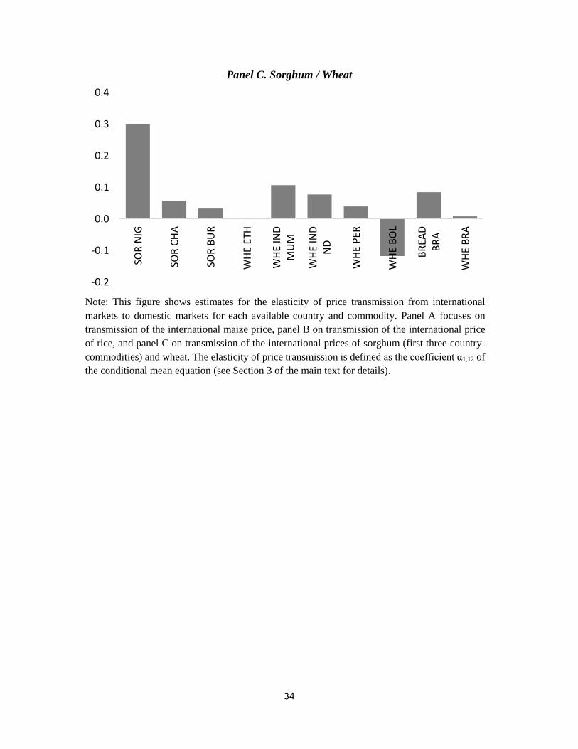
Panel C of Table 2 shows the price transmission for three sorghum markets and seven
wheat markets. None of the three sorghum markets (Burundi, Chad, and Nigeria) have statistically
significant links to world sorghum markets. This is expected since international trade in sorghum
is negligible in all three countries (see Table 3). In the case of wheat, two of the seven markets
show a statistically significant link with world wheat markets: Mumbai, India and Lima, Peru. It
is not surprising that wheat prices in Lima are linked to world markets given the countries heavy
reliance on imported wheat. On the other hand, it is somewhat surprising to find a link between
Mumbai prices and world prices, given that India is (on average) self-sufficient in wheat. It should
be noted, however, that the Mumbai is a wheat deficit region at some distance from the wheat
surplus zone in the Punjab. In contrast, New Delhi is quite close to the Punjabi wheat zone. Brazil
and Bolivia are depend heavily on wheat imports, but Argentina is the main source of wheat and
Argentinian prices are imperfectly integrated with US wheat prices, used as the benchmark for
world prices in this study. The lack of linkage between Ethiopian wheat prices and world wheat
prices is probably due to the large (but variable) share of wheat imports that are in the form of food
aid, thus less driven by market forces.
5.2 Volatility transmission

17
In this section, we describe our price volatility transmission estimates from international
commodity markets to domestic food markets across countries and commodities. Due to space
limitations, we only report in the second panel of Table 2 the estimated coefficients of the BEKK
model describing the conditional variance equation of domestic markets (specified in equation
(3)).7 The lower panel of Table 3 also reports different residual diagnostic tests, which generally
support the adequacy of BEKK model specification. In particular, the Ljung-Box, Lagrange
Multiplier (LM), and Hosking Multivariate Portmanteau test statistics for up to 6 and 12 lags show
no or weak evidence of autocorrelation, ARCH effects, and cross-correlation in the standardized
squared residuals of the estimated models.
First, we assess the reliability of our estimations by comparing model predictions to sample
price volatility statistics (sample standard deviation of domestic price returns) for each domestic
price.8 For model predictions of price returns volatilities we use i) the average of predicted
conditional standard deviations of price returns and ii) the estimated steady-state (or unconditional)
price return volatility.9
Figure A.1 in the Appendix compares the sample and model estimates of domestic price
volatilities. Sample data indicates that maize volatility is on average larger than rice and wheat
volatility. Average sample maize volatility is 10.4% while for rice and wheat are 4.7% and 4.8%,
respectively. Across regions African countries have the highest sample volatilities (average of
7 Wald joint tests indicate that in several cases there are immediate innovation and persistence effects from
international to domestic markets. We discuss in more detail below volatility transmission from international to
domestic markets.
8 The sample volatility is equal to (ℎ11𝑠𝑎𝑚𝑝𝑙𝑒
)0.5
= √∑ (𝑟𝑡−�̅�)2𝑛
𝑡=1
𝑛.
9 The average of predicted conditional volatilities is equal to ℎ11̂̅̅ ̅̅ =
∑ ℎ̂11.𝑡0.5𝑛
𝑡=1
𝑛 while the steady–state volatility
(ℎ11𝑆𝑆)0.5 satisfies GHGCCH SSSS '' .

18
11.3%) while in Asia and Latin America the averages are less than half of the African average.
Our estimated steady-state and predicted volatilities yield similar conclusions when comparing
commodities and regions. When we compare steady-state volatility with sample volatility, the
former is consistently lower than the latter. In particular, steady-state volatility estimates are on
average 60% of the sample estimates. This is expected as steady-state estimates reflect the standard
deviations to be reached over time in the absence of shocks. This finding is also consistent with
results reported by Gardebroek, Hernandez, and Robles (2014).
When we compare average predicted volatility with sample volatility, we also observe that
our estimated models perform reasonably well. The ratio of the average predicted volatility to the
sample volatility is on average 0.99 for the full set of countries and commodities. and our average
predicted volatilities further reaffirm that on average maize price volatility is much more volatile
(more than two times larger) than rice and wheat price volatility.
To obtain estimates for the degree of volatility transmission from international markets to
domestic markets we carry out the following two steps for each estimated model (one per
country/commodity):
1. We estimate the size of a shock in the international market (𝜀2̅) such that the steady-state
standard deviation of the international price return increases in one percent after one period:
√𝐻1,22(𝜀2̅) − √𝐻0,22
√𝐻0,22
= 0.01
2. We introduce shock 𝜀2̅ in expression (2) and estimate the percentage change in the standard
deviation of the domestic price return (with respect to its steady-state value) and compute
our volatility transmission VT indicator according to:

19
𝑉𝑇 = √𝐻1,11 − √𝐻0,11
√𝐻0,11
÷ 0.01
In other words, our volatility transmission indicator shows the reaction (after one period
and assuming the system is on steady-state) of the domestic volatility (standard deviation of price
return) to a shock in the international market. If our volatility transmission indicator is equal to
one it means that the domestic volatility increases in one period in the same proportion as the
international price volatility, after introducing a shock in the international market.
We present our volatility transmission estimates for each country and commodity in Figure
6 and aggregated median and frequencies across commodities and regions in Table A.3 in the
Appendix. Overall most of our estimates are within reasonable values.10
[Insert Figure 6]
An approximate measure of the statistical significance of the relationship between
international price volatility and domestic volatility is given by the Wald test for the joint
significance of α21 and g21 in the conditional variance equation (see Table 2). α21 represents the
short-term effect of an international price shock on domestic volatility, while g21 represents the
short-term effect of changes in international price volatility on domestic volatility.
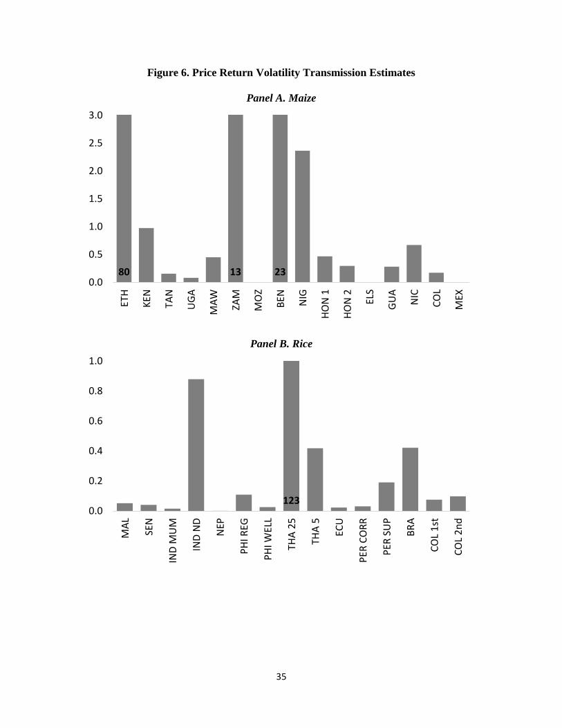
In the case of maize, 4 of the 16 Wald tests reject the null hypothesis that both coefficients
are zero: Benin, Ethiopia, Nigeria, and Colombia. The linkage between international and domestic
volatility is easy to understand in the case of Colombia, which imports 64% of its maize
requirements over the period under study. The linkage for the other three countries is unexpected,
given that all three rely on imports for less than 2% of domestic requirements (see Table 3).
10 Only in 6 out of 41 cases our estimates show extreme values larger than 10.

20
In the case of rice, 7 of the 15 markets show evidence of a statistically significant spillover
from international volatility to domestic volatility (see Table 2). This is expected in the case of
Senegal, which imported 82% of its domestic requirements, and the two prices in Thailand, which
exported more than 40% of its production (see Table 3). Similarly, the lack of linkage in India,
Nepal, Brazil, and Ecuador is explained by small contribution of rice imports in these countries.
More surprising is the volatility spillover in Colombia and Peru, where rice imports meet less than
7% of local demand.
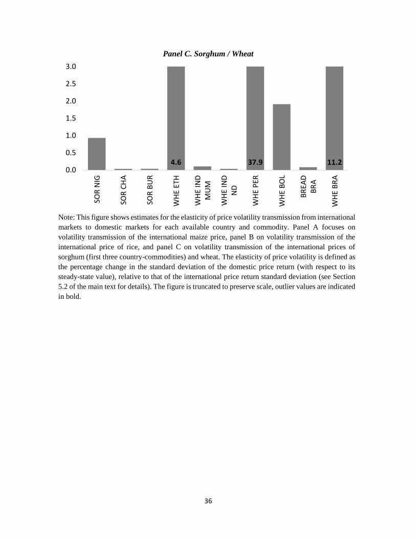
In the case of sorghum, one of the three prices shows signs of a statistically significant
spillover in volatility from international markets: Burundi (see Table 2). This is surprising given
that Burundi is landlocked and has virtually no sorghum imports from world markets. The lack of
spillover for Chad and Nigeria are, however, expected given the negligible volumes of traded
sorghum.
Wheat markets in developing countries appear to be relatively sensitive to volatility in
international wheat markets. All seven of the markets tests showed evidence of a statistically
significant link between international and domestic price volatility (see Table 2). This is expected
in the case of Peru, Bolivia, and Brazil, given their reliance on imported wheat for more than half
of local consumption, and understandable in the case of Ethiopia, which imports 32% of its
requirements (see Table 3). On the other hand, India is largely self-sufficient in wheat in most
years, so the volatility linkage with world wheat markets is harder to explain.
5.3 Conditional correlations
Lastly, we are interested in examining whether the dynamic price relationship between
domestic and international markets has changed in recent years, particularly after the global food

21
price crisis of 2007-2008. From the BEKK model, we can recover time-varying conditional
correlations between the price returns of each domestic market and the international market. This
correlation is given by
tt
t
t
hh
h
,22,11
,12
,12ˆˆ
ˆˆ , where th ,11
ˆ and th ,22ˆ are the estimated conditional
variance equations and th ,12ˆ is the covariance equation. We then run separate regressions of these
recovered conditional correlations on a trend term, trend squared and a dummy shifter for the
period July 2007 onwards, as mid-2007 was the period where the crisis was felt most (food prices
peaked).
Table 4 reports the number of cases where we find a statistically significant change after
June 2007 in the degree of co-movement between domestic and international price returns by
commodity and region (at the 95% confidence level). Overall, we do not observe major changes
in the dynamic interrelationship between domestic and international price returns after the food
price crisis. Only in nine cases (out of 41) there is a positive shift in the domestic-international
conditional correlation and in two cases there is a negative shift. The two negative cases are in
Africa (maize in Mozambique and wheat in Ethiopia), while the nine positive cases are distributed
four in Asia (rice in Philippines (well milled) and Thailand (25% broken) and wheat in Mumbai
and New Delhi), four in Latin America (rice in Ecuador and Peru (milled, standard), maize in
Honduras and wheat in Peru), and one in Africa (maize in Ethiopia). Figure A.2 in the Appendix
further reports the median change in the domestic-international correlations by commodity and
region, confirming that the shifts were generally small, except for rice with a median shift of 10
percentage points.
[Insert Table 4]

22
6. Conclusions
Food price volatility in developing countries is economically and politically important. In
these economies a large share of household budgets is spent on food, so food price levels and
volatility have a direct and large impact on welfare. Food price volatility particularly affects poor,
small-scale farmers who rely on crop sales for a significant part of their income. It is also likely
to inhibit agricultural investment and reduce the growth in agricultural productivity, with long-run
implications for poor consumers and farmers. Hence, it is important to better understand the
sources of food price volatility and whether it is mostly transmitted from international agricultural
commodity markets or largely determined by domestic factors. This in turn can help design better
global, regional, and domestic policies to cope with excessive food price volatility and to protect
the most vulnerable groups.
The objective of this paper is to estimate the extent of both grain price and volatility
transmission from world markets to local markets in developing countries, in a context where
volatility interactions has not been largely analyzed in the literature. In particular, we focus on the
effect of the world price of maize, rice, wheat, and sorghum on 41 prices of grain products in 27
countries in Latin America, Africa, and Asia. The price data are monthly, and most cover the
period from January 2000 to December 2013. The analysis is based on a MGARCH approach
using a BEKK model.
In terms of price transmission in levels, we only observe lead-lag relationships from
international to domestic markets in few cases. Only 6 international-domestic price elasticities (out
of 41) are statistically significant. In terms of volatility transmission, however, we observe more
interactions across markets. We propose as a volatility transmission estimator (or elasticity) one
that shows the reaction (after one period and assuming the system is on steady-state) of the

23
domestic price volatility (the standard deviation of price returns) given a one-percent shock in
international price volatility of the commodity. We find that most of our elasticity estimates are
within reasonable values.
Maize markets in developing countries are the least susceptible to volatility in international
markets, with just one-quarter of them (4 of 16) showing evidence of a statistically significant
effect. Rice markets appear to be more sensitive to volatility in international markets, with almost
half the markets tested (7 of 15) having statistically significant spillover. And wheat markets were
the most sensitive to international price volatility, with a significant linkage in all seven markets
tested. In general terms, this pattern reflects the fact that most of the countries in our sample are
relatively self-sufficient in maize: on average, net trade represents 16% of domestic use. In
contrast, these countries are more dependent on rice trade (average 38%) and most reliant on
international trade in wheat (average 78%).
These patterns extend to individual markets. Colombia is heavily dependent on maize
imports and is one of just four markets with significant volatility linkages. Senegal and Thailand
are both deeply involved in rice trade, as importer and exporter respectively, and both show
volatility spillover from world markets. Similarly, Brazil, Bolivia, Peru, and Ethiopia rely heavily
on wheat imports and show transmission of volatility from world markets.
At the same time, there are a number of exceptions to these patterns. Some countries with
little trade in a commodity have domestic price volatility that appears linked to international
volatility. Examples include maize in Ethiopia, rice in Peru, sorghum in Burundi, and wheat in
India. One hypothesis is that the behavior of local traders or government trading enterprises
monitor international markets and are prompted by international volatility to respond in ways that
contribute to local volatility even in the absence of direct trade effects. Another possibility is that

24
price volatility is actually being transmitted through closely related staple grain markets for which
there is trade. Testing these hypotheses would be a fruitful direction for future research.

25
References
Abdulai, A., 2000. “Spatial price transmission and asymmetry in the Ghanaian maize market.”
Journal of Development Economics 63: 327–349.
Ai, C., A. Chatrath, and F. Song, 2006. “On the Co-movement of Commodity Prices.” American
Journal of Agricultural Economics 88: 574–588.
Baba, Y., R. Engle, D. Kraft, and K.F Kroner, 1990. “Multivariate simultaneous generalized
ARCH.” Mimeo, Department of Economics, University of California, San Diego.
Baulch, B., 1997. “Transfer costs, spatial arbitrage and testing for food market integration.”
American Journal of Agricultural Economics 79 (May): 477-87.
Bauwens, L., S. Laurent, and J.V.K. Rombouts, 2006. “Multivariate GARCH models: A survey.”
Journal of Applied Econometrics 21: 79-109.
Beckmann, J., and R. Czudaj, 2014. “Volatility transmission in agricultural futures markets.”
Economic Modelling 36: 541–546.
Conforti, P., 2004. “Price transmission in selected agricultural markets.” Commodity and Trade
Policy Research Working Paper No 7. Rome: Food and Agriculture Organisation.
Deb, P., P. K. Trivedi, and P. Varangis, 1996. “The Excess Co-movement of Commodity Prices
Reconsidered.” Journal of Applied Econometrics 11: 275–291.
Engle, R., and F.K. Kroner, 1995. “Dynamic conditional correlation-a simple class of multivariate
GARCH models.” Journal of Business and Economics Statistics 20: 339–350.
FAO (Food and Agriculture Organization). 2014. Food Balance Sheets. FAO, Rome.
(http://faostat3.fao.org/download/FB/FBE/S).
Gallagher, L., and C. Twomey, 1998. “Identifying the source of mean and volatility spillovers in
Irish equities: a multivariate GARCH analysis.” Economic and Social Review 29: 341–356.
Gardebroek, C., and M.A. Hernandez, 2013. “Do energy prices stimulate food price volatility?
Examining volatility transmission between US oil, ethanol and corn market.” Energy
Economics 40: 119-129.
Gardebroek, C., M.A. Hernandez, and M. Robles, 2014. “Market interdependence and volatility
transmission among major crops.” Agricultural Economics, forthcoming.
Gilbert, C.L., 2010. “How to understand high food prices.” Journal of Agricultural Economics 61:
398–425.

26
Hernandez, M.A., R. Ibarra, and D.R. Trupkin, 2014. “How far do shocks move across borders?:
Examining volatility transmission in major agricultural futures markets.” European Review
of Agricultural Economics 41(2): 301–325.
Le Pen, Y., and B. Sévi, 2010. “Revisiting the Excess Co-movement of Commodity Prices in a
Data Rich Environment.” Economics Papers from University Paris Dauphine, Paris
Dauphine University, France.
Lutz, C., W. E. Kuiper, and a. van Tilburg, 2006. “Maize Market Liberalisation in Benin: A Case
of Hysteresis.” Journal of African Economies 16(1): 102-133.
Meyer, J., and S. von Cramon-Taubadel, 2004. “Asymmetric price transmission: A survey.”
Journal of Agricultural Economics 55(3): 581–611.
Minot, N., 2010. “Transmission of World Food Price Changes to African Markets and its Effect
on Household Welfare.” IFPRI discussion papers 1059, International Food Policy Research
Institute, Washington DC.
Minot, N., 2014. “Food price volatility in sub-Saharan Africa: Has it really increased?” Food
Policy 45: 45-56.
Moser, C., C. Barrett, and B. Minten, 2009. “Spatial integration at multiple scales: Rice markets
in Madagascar.” Agricultural Economics 40: 281–294.
Mundlak, Y., and D. Larson, 1992. “On the transmission of world agricultural prices.” The World
Bank Economic Review 6(3): 399–422.
Myers, R., 2008. “Evaluating the efficiency of inter-regional trade and storage in Malawi maize
markets.” Report for the World Bank. East Lansing, Mich., U.S.A.: Michigan State
University.
Negassa, A., and R. Myers, 2007. “Estimating policy effects on spatial market efficiency: An
extension to the parity bounds model.” American Journal of Agricultural Economics 89:
338–352.
Pindyck, R.S., and J.J. Rotemberg, 1990. “The Excess Co-movement of Commodity Prices.”
Economic Journal 100: 1173–1189.
Quiroz, J., and R. Soto, 1995. “International price signals in agricultural prices: Do governments
care?” Documento de investigacion 88. Santiago, Chile: ILADES Postgraduate Economics
Program, Georgetown University.
Robles, M., and M. Torero, 2010. “Understanding the impact of high food prices in Latin
America.” Economia 10(2), 117-164.

27
Saadi, H., 2010. “Price co-movement in international markets and their impacts on price
dynamics.” In: Piot-Lepetit, I. and M’Barek, R. (Eds.), Methods to Analyse Agricultural
Commodity Price Volatility. Springer Science, Chapter 9.
Seale, J.L., A. Regmi, and J. Bernstein, 2003. “International Evidence on Food Consumption
Patterns.” Technical Bulletin No. 33580, United States Department of Agriculture,
Economic Research Service.
Silvennoinen, A., and T. Teräsvirta, 2009. “Multivariate GARCH models.” In: Andersen, T.G.,
R.A. Davis, J.-P Kreiß, and T. Mikosch (Eds.), Handbook of Financial Time Series.
Springer, Berlin, 201-229.
Rashid, S., 2004. “Spatial Integration of Maize Markets in Post-liberalised Uganda.” Journal of
African Economies 13(1): 102-133.
Van Campenhout, B., 2007. “Modeling trends in food market integration: Method and an
application to Tanzanian maize markets.” Food Policy 32: 112–127.
Zhao, J., and B. Goodwin, 2011. “Volatility spillovers in agricultural commodity markets: An
application involving implied volatilities from options markets.” Paper prepared for
presentation at the Agricultural and Applied Economics Association’s 2011 Annual
Meeting.

28
Figure 1. International Commodity Prices - 2000-2014
Note: This figure shows the evolution of the monthly international prices of maize, rice,
sorghum, and wheat during the 2000-2014 period. Prices are expressed in US$ per tonne.
0
100
200
300
400
500
600
700
800P
rice
(U
S$ /
to
nn
e)
Maize Rice Sorghum Wheat

29
Figure 2. Volatility of International Grain Prices (2-year moving window) - 2000-2014
Note: This figure shows the evolution of the volatility of monthly international prices of maize,
rice, sorghum, and wheat during the 2000-2014 period. The volatility for every month is
calculated as the standard deviation of the monthly price returns observed during that and the
previous 23 months.
0
0.02
0.04
0.06
0.08
0.1
0.12
0.14
Vo
lati
lity
(std
dev
iati
on
of
pri
ce r
etu
rns)
Maize Rice Sorghum Wheat

30
Figure 3. Volatility of International Grain Prices before and after the 2007-2008 Crisis
Note: This figure shows the volatility of monthly international prices of maize, rice, sorghum,
and wheat before and after the 2007-2008 food crisis. The “before” period spans 2000-2006 while
the “after” period spans 2009-2014. The volatility for each period is calculated as the standard
deviation of the observed monthly price returns for each commodity.
0
0.01
0.02
0.03
0.04
0.05
0.06
0.07
0.08
Maize Rice Sorghum Wheat
Vo
lati
lity
(std
dev
iati
on
of
pri
ce r
etu
rns)
2000-2006 2009-2014

31
Figure 4. Volatility (2-year moving window) of Domestic and International Prices
Panel A. Maize
Panel B. Rice
Panel C. Sorghum
0.0
0.1
0.2
0.3
2002m1 2004m1 2006m1 2008m1 2010m1 2012m1 2014m1
0.00
0.05
0.10
0.15
0.20
1996m1 1998m1 2000m1 2002m1 2004m1 2006m1 2008m1 2010m1 2012m1 2014m1
0.05
0.10
0.15
0.20
0.25
2004m1 2006m1 2008m1 2010m1 2012m1 2014m1
Vo
lati
lity
(std
dev
iati
on
of
pri
ce r
etu
rns)
V
ola
tilit
y (s
td d
evia
tio
n o
f p
rice
ret
urn
s)
Vo
lati
lity
(std
dev
iati
on
of
pri
ce r
etu
rns)

32
Panel D. Wheat
Note: This figure shows the evolution of the volatility of monthly domestic and international prices of
maize, rice, sorghum, and wheat during the 2000-2014 period. The volatility for every month is
calculated as the standard deviation of the monthly price returns observed during that and the previous
23 months. The line in bold represents the volatility of each international price series.
0.00
0.05
0.10
0.15
2000m1 2002m1 2004m1 2006m1 2008m1 2010m1 2012m1 2014m1
Vo
lati
lity
(std
dev
iati
on
of
pri
ce r
etu
rns)

33
Figure 5. Price Return Transmission Estimates (in Levels)
Panel A. Maize
Panel B. Rice
-0.2
-0.1
0.0
0.1
0.2
0.3
0.4ET
H
KEN
TAN
UG
A
MA
W
ZAM
MO
Z
BEN NIG
HO
N 1
HO
N 2
ELS
GU
A
NIC
CO
L
MEX
-0.3
-0.2
-0.1
0.0
0.1
0.2
MA
L
SEN
IND
MU
M
IND
ND
NEP
PH
I REG
PH
I WEL
L
THA
25
THA
5
ECU
PER
CO
RR
PER
SU
P
BR
A
CO
L 1
st
CO
L 2
nd
34
Panel C. Sorghum / Wheat
Note: This figure shows estimates for the elasticity of price transmission from international
markets to domestic markets for each available country and commodity. Panel A focuses on
transmission of the international maize price, panel B on transmission of the international price
of rice, and panel C on transmission of the international prices of sorghum (first three country-
commodities) and wheat. The elasticity of price transmission is defined as the coefficient α1,12 of
the conditional mean equation (see Section 3 of the main text for details).
-0.2
-0.1
0.0
0.1
0.2
0.3
0.4
SOR
NIG
SOR
CH
A
SOR
BU
R
WH
E ET
H
WH
E IN
DM
UM
WH
E IN
DN
D
WH
E P
ER
WH
E B
OL
BR
EAD
BR
A
WH
E B
RA
35
Figure 6. Price Return Volatility Transmission Estimates
Panel A. Maize
Panel B. Rice
80 13 230.0
0.5
1.0
1.5
2.0
2.5
3.0ET
H
KEN
TAN
UG
A
MA
W
ZAM
MO
Z
BEN NIG
HO
N 1
HO
N 2
ELS
GU
A
NIC
CO
L
MEX
1230.0
0.2
0.4
0.6
0.8
1.0
MA
L
SEN
IND
MU
M
IND
ND
NEP
PH
I REG
PH
I WEL
L
THA
25
THA
5
ECU
PER
CO
RR
PER
SU
P
BR
A
CO
L 1
st
CO
L 2
nd
36
Panel C. Sorghum / Wheat
Note: This figure shows estimates for the elasticity of price volatility transmission from international
markets to domestic markets for each available country and commodity. Panel A focuses on
volatility transmission of the international maize price, panel B on volatility transmission of the
international price of rice, and panel C on volatility transmission of the international prices of
sorghum (first three country-commodities) and wheat. The elasticity of price volatility is defined as
the percentage change in the standard deviation of the domestic price return (with respect to its
steady-state value), relative to that of the international price return standard deviation (see Section
5.2 of the main text for details). The figure is truncated to preserve scale, outlier values are indicated
in bold.
4.6 37.9 11.20.0
0.5
1.0
1.5
2.0
2.5
3.0
SOR
NIG
SOR
CH
A
SOR
BU
R
WH
E ET
H
WH
E IN
DM
UM
WH
E IN
DN
D
WH
E P
ER
WH
E B
OL
BR
EAD
BR
A
WH
E B
RA

37
Table 1. Summary Statistics and Selected Normality, Autocorrelation, and Stationarity
Tests
Panel A. Domestic price series
Maize Rice Sorghum Wheat Total
Number of domestic price series 16 15 3 7 41
Mean price returns 0.42% 0.33% 0.47% 0.46% 0.40%
% of series with kurtosis > 3 100.0% 100.0% 100.0% 100.0% 100.0%
% of series rejecting Jarque-Bera test's H0 93.8% 100.0% 100.0% 100.0% 97.6%
% of series rejecting Ljung-box test's H0
on squared returns (5 lags) 31.3% 66.7% 0.0% 71.4% 48.8%
% of series rejecting Ljung-box test's H0
on squared returns (10 lags) 31.3% 73.3% 33.3% 71.4% 53.7%
% of series rejecting AC Q test's H0
on squared returns (first lag) 37.5% 73.3% 33.3% 71.4% 56.1%
% of series rejecting AC Q test's H0
on squared returns (second lag) 43.8% 80.0% 33.3% 85.7% 63.4%
% of series rejecting ADF test's H0
on logarithm of price in levels (5 lags) 56.3% 13.3% 0.0% 57.1% 36.6%
% of series rejecting ADF test's H0
on price returns (5 lags) 100.0% 100.0% 100.0% 100.0% 100.0%
Panel B. International price series
Maize Rice Sorghum Wheat
Mean price returns 0.52% 0.39% 0.54% 0.62%
Standard deviation of price returns 6.44% 6.18% 6.74% 6.65%
Jarque-Bera statistic 28.68* 273.10* 39.46* 39.37*
Kurtosis 4.84 9.15 5.27 5.11
Ljung-box statistic on squared returns (5 lags) 1.58 53.74* 4.42 7.25
Ljung-box statistic on squared returns (10
lags) 11.86 80.14* 8.71 11.86
AC Q statistic on squared returns (First lag) 0.09 0.35* 0.08 0.17*
AC Q statistic on squared returns (Second lag) 0.03 0.34 0.01 0.09*
ADF statistic - Logarithm of price in levels (5
lags) -1.40 -1.58 -1.47 -1.78
ADF statistic - Price returns (5 lags) -5.88* -5.74* -5.74* -4.68*
Note: This table presents summary statistics and selected normality, autocorrelation, and stationarity tests
for domestic (panel A) and international (panel B) price return series for maize, rice, sorghum, and wheat.

38
Table 2. Selected Model Results and Residual Tests
BEN ETH KEN MAW MOZ NIG TAN UGA ZAM ELS GUA HON 1 HON 2 MEX NIC COL
Conditional Mean Equation
Model VAR VEC VEC VAR VEC VAR VAR VEC VAR VAR VEC VAR VEC VEC VEC VAR
No. of lags 1 0 0 1 0 1 2 0 1 1 0 2 1 0 0 1
α0 0.006 -0.003 -0.001 0.002 -0.001 0.010 0.003 -0.001 -0.001 0.002 -0.002 0.003 0.000 0.001 0.000 -0.001
(0.012) (0.009) (0.007) (0.019) (0.009) (0.012) (0.009) (0.013) (0.009) (0.005) (0.006) (0.006) (0.006) (0.003) (0.009) (0.006)
α1,11 0.019 0.179 -0.015 0.221 -0.019 0.172 0.206 0.464 0.230
(0.093) (0.091) (0.094) (0.084) (0.084) (0.077) (0.083) (0.071) (0.078)
α1,12 0.190 0.319 0.279 -0.134 0.103 0.012 0.244 0.069 0.133
(0.179) (0.267) (0.174) (0.145) (0.135) (0.081) (0.100) (0.092) (0.092)
Conditional Variance Equation
c11 11.813 -0.029 3.694 19.345 1.676 4.373 8.508 -6.674 0.211 0.613 0.629 5.493 6.199 2.267 -5.438 2.336
(1.661) (0.095) (2.901) (2.291) (2.074) (2.006) (2.345) (3.068) (0.260) (1.365) (1.579) (1.617) (0.662) (1.216) (7.301) (2.101)
a11 0.346 0.530 -0.250 0.336 0.622 -0.105 0.475 0.683 -0.707 0.408 0.798 -0.938 0.409 0.675 0.789 0.279
(0.105) (0.145) (0.574) (0.165) (0.328) (0.196) (0.141) (0.168) (0.399) (0.706) (0.224) (0.342) (0.129) (0.181) (0.222) (0.196)
a21 -0.807 -0.198 -0.409 0.539 -0.028 0.738 -0.260 0.102 -0.146 -0.012 0.084 0.111 0.162 -0.005 -0.290 0.138
(0.381) (0.114) (0.418) (0.257) (0.112) (0.278) (0.177) (0.275) (0.112) (0.065) (0.075) (0.195) (0.092) (0.108) (0.173) (0.135)
g11 0.002 0.897 -0.785 0.001 -0.837 0.855 -0.408 0.565 0.807 -0.765 0.656 -0.059 0.000 -0.001 -0.384 0.831
(0.016) (0.053) (0.376) (0.012) (0.095) (0.134) (0.196) (0.241) (0.101) (0.112) (0.189) (0.237) (0.015) (0.204) (0.202) (0.193)
g21 0.000 -0.102 -0.434 0.000 -0.430 0.067 -0.446 -0.918 -0.388 0.606 -0.300 -0.077 0.000 0.358 0.688 -0.459
(0.011) (0.102) (1.015) (0.033) (0.296) (0.553) (0.433) (0.495) (0.353) (0.383) (0.194) (0.366) (0.009) (0.200) (1.225) (0.070)
ν 4.314 3.717 4.231 4.728 2.813 3.667 3.722 7.037 3.665 4.600 6.029 3.730 6.207 4.051 4.413 3.744
(1.287) (0.924) (1.835) (1.209) (0.782) (0.919) (0.821) (2.587) (1.746) (1.570) (2.768) (1.238) (1.702) (0.897) (0.972) (0.851)
Wald test for presence of innovation and persistence effects from international to domestic market (H 0 : a 21 = g 21 = 0)
Chi-squared 9.083 7.399 3.384 4.429 3.507 12.159 5.663 5.408 2.520 2.506 2.469 0.423 3.287 5.307 4.131 43.095
p -Value 0.011 0.025 0.184 0.109 0.173 0.002 0.059 0.067 0.284 0.286 0.291 0.809 0.193 0.070 0.127 0.000
Ljung-Box test for autocorrelation (H 0 : no autocorrelation in squared residuals)
LB(6) 2.522 16.574 8.201 6.945 10.494 10.843 3.668 3.973 7.967 2.477 3.981 9.137 2.020 4.971 6.578 14.003
p -Value 0.866 0.011 0.224 0.326 0.105 0.093 0.722 0.680 0.241 0.871 0.679 0.166 0.918 0.547 0.362 0.030
LB(12) 10.152 32.112 15.799 22.446 22.996 20.540 8.285 8.196 13.254 12.784 31.099 30.716 12.912 14.728 21.938 20.610
p -Value 0.603 0.001 0.201 0.033 0.028 0.058 0.763 0.770 0.351 0.385 0.002 0.002 0.375 0.257 0.038 0.056
Lagrange multiplier (LM) test for ARCH residuals (H 0 : no ARCH effects)
LM(6) 1.002 2.442 4.045 1.104 0.654 2.200 2.807 1.833 8.384 3.022 6.344 3.488 2.904 4.138 3.508 0.549
p -Value 0.986 0.875 0.671 0.981 0.995 0.900 0.833 0.934 0.211 0.806 0.386 0.746 0.821 0.658 0.743 0.997
LM(12) 6.154 5.542 6.436 4.294 2.008 4.113 9.094 4.804 8.461 7.299 13.614 4.758 5.117 6.745 6.885 2.162
p -Value 0.908 0.937 0.893 0.978 0.999 0.981 0.695 0.964 0.748 0.837 0.326 0.966 0.954 0.874 0.865 0.999
Hosking Multivariate Portmanteau test for cross-correlation (H 0 : no cross-correlation in squared residuals)
M(6) 12.367 11.711 18.921 46.859 5.756 9.724 9.894 9.141 30.430 17.910 15.418 10.739 14.110 15.136 9.683 4.389
p -Value 0.975 0.983 0.756 0.003 1.000 0.996 0.995 0.997 0.171 0.807 0.908 0.991 0.944 0.917 0.996 1.000
M(12) 51.848 30.398 31.940 73.003 24.924 34.904 44.511 34.225 55.156 43.978 47.272 34.011 34.071 41.570 44.185 38.139
p -Value 0.326 0.978 0.964 0.011 0.998 0.921 0.617 0.933 0.222 0.638 0.503 0.937 0.936 0.732 0.630 0.845
Log Likelihood -861.8 -770.0 -1117.1 -892.6 -968.9 -804.3 -975.0 -1034.8 -977.9 -1017.8 -637.3 -915.4 -926.0 -989.5 -1097.6 -969.2
No. of Obs. 123 120 168 120 144 123 144 144 144 161 101 148 148 171 161 154
MAIZE

39
MAL SENIND
MUM
IND
NDNEP
PHI
REG
PHI
WELLTHA 25 THA 5 BRA
COL
1st
COL
2ndECU
PER
CORR
PER
SUP
Conditional Mean Equation
Model VEC VAR VAR VEC VAR VEC VEC VAR VAR VEC VAR VAR VEC VAR VAR
No. of lags 1 4 2 1 3 1 1 2 2 1 3 3 1 2 2
α0 0.002 -0.001 0.003 0.002 0.001 0.002 0.002 0.002 0.003 0.002 0.002 0.002 0.005 0.001 0.001
(0.005) (0.007) (0.002) (0.002) (0.007) (0.003) (0.003) (0.004) (0.004) (0.004) (0.003) (0.003) (0.003) (0.001) (0.001)
α1,11 0.069 -0.498 0.227 0.193 0.484 0.135 0.219 0.421 0.416 0.203 0.347 0.316 -0.153 0.280 0.335
(0.093) (0.095) (0.077) (0.078) (0.099) (0.078) (0.079) (0.132) (0.110) (0.076) (0.078) (0.078) (0.097) (0.067) (0.066)
α1,12 0.043 0.105 -0.064 -0.015 -0.267 0.113 0.085 0.095 0.078 0.148 0.018 0.003 0.055 0.019 0.025
(0.082) (0.141) (0.045) (0.034) (0.122) (0.054) (0.046) (0.143) (0.120) (0.071) (0.063) (0.070) (0.041) (0.029) (0.019)
Conditional Variance Equation
c11 4.243 1.638 0.008 0.017 2.357 2.006 0.743 1.444 1.818 3.029 1.167 1.852 0.615 1.065 0.767
(0.908) (1.203) (0.025) (0.023) (2.070) (0.966) (0.257) (0.369) (0.582) (1.392) (0.705) (0.651) (0.229) (0.369) (0.157)
a11 0.440 0.364 0.091 0.629 0.343 0.254 -0.278 0.487 0.813 0.312 -0.039 0.061 0.660 0.520 0.474
(0.459) (0.105) (0.096) (0.122) (0.111) (0.135) (0.084) (0.134) (0.161) (0.262) (0.084) (0.078) (0.193) (0.134) (0.124)
a21 0.252 0.232 0.044 -0.070 0.011 0.204 0.115 0.118 -0.303 -0.292 -0.218 0.179 0.018 -0.047 -0.064
(0.323) (0.128) (0.038) (0.057) (0.177) (0.076) (0.083) (0.087) (0.120) (0.186) (0.071) (0.094) (0.039) (0.036) (0.018)
g11 -0.123 0.907 0.997 0.854 0.896 0.742 0.943 0.952 0.854 0.585 0.890 0.804 0.762 0.676 -0.678
(0.561) (0.067) (0.011) (0.046) (0.116) (0.266) (0.026) (0.102) (0.139) (0.459) (0.102) (0.070) (0.106) (0.152) (0.087)
g21 0.109 -0.473 -0.031 0.037 -0.012 -0.353 -0.015 -0.267 -0.630 0.530 0.151 -0.370 -0.007 -0.011 -0.042
(0.309) (0.152) (0.014) (0.022) (0.105) (0.111) (0.024) (0.059) (0.164) (0.233) (0.088) (0.100) (0.060) (0.049) (0.064)
ν 3.957 5.166 5.101 4.420 5.229 9.175 5.016 8.985 8.816 13.610 132.498 10.599 7.369 4.101 8.132
(1.487) (1.336) (1.825) (1.114) (2.500) (3.853) (1.059) (3.800) (3.785) (10.981) (330.799) (6.190) (4.910) (0.766) (2.889)
Wald test for presence of innovation and persistence effects from international to domestic market (H 0 : a 21 = g 21 = 0)
Chi-squared 2.198 9.734 5.435 2.956 0.013 12.546 2.886 23.040 21.981 5.548 9.335 18.338 0.211 2.025 12.704
p -Value 0.333 0.008 0.066 0.228 0.994 0.002 0.236 0.000 0.000 0.062 0.009 0.000 0.900 0.363 0.002
Ljung-Box test for autocorrelation (H 0 : no autocorrelation in squared residuals)
LB(6) 6.794 13.517 8.398 0.821 8.533 2.908 3.741 4.675 4.998 3.695 6.004 5.095 7.670 1.752 5.119
p -Value 0.340 0.036 0.210 0.991 0.202 0.820 0.712 0.586 0.544 0.718 0.423 0.532 0.263 0.941 0.529
LB(12) 10.996 20.869 13.984 4.935 15.420 8.230 9.706 12.043 13.360 10.083 11.055 12.741 10.466 6.336 9.857
p -Value 0.529 0.052 0.302 0.960 0.219 0.767 0.642 0.442 0.343 0.609 0.524 0.388 0.575 0.898 0.629
Lagrange multiplier (LM) test for ARCH residuals (H 0 : no ARCH effects)
LM(6) 20.121 6.745 2.583 2.040 1.348 2.239 7.008 2.669 2.198 2.379 9.819 3.467 6.180 2.365 2.191
p -Value 0.003 0.345 0.859 0.916 0.969 0.896 0.320 0.849 0.901 0.882 0.132 0.748 0.403 0.883 0.901
LM(12) 22.214 15.907 10.044 5.465 3.407 5.564 9.824 4.293 6.550 7.305 10.994 4.501 9.726 4.690 4.816
p -Value 0.035 0.196 0.612 0.941 0.992 0.936 0.631 0.978 0.886 0.837 0.529 0.973 0.640 0.968 0.964
Hosking Multivariate Portmanteau test for cross-correlation (H 0 : no cross-correlation in squared residuals)
M(6) 31.893 16.927 14.748 43.910 11.413 14.392 32.630 21.456 15.355 17.461 40.464 16.529 34.438 41.278 40.700
p -Value 0.130 0.852 0.928 0.008 0.986 0.937 0.112 0.612 0.910 0.828 0.019 0.868 0.077 0.016 0.018
M(12) 46.515 32.029 44.182 59.293 22.062 32.705 41.889 38.219 33.908 31.333 58.757 33.401 52.108 52.395 63.919
p -Value 0.534 0.963 0.630 0.127 1.000 0.955 0.720 0.843 0.938 0.970 0.137 0.946 0.317 0.307 0.062
Log Likelihood -690.8 -695.5 -872.1 -851.1 -641.2 -914.9 -886.4 -865.9 -890.0 -977.4 -908.6 -931.3 -546.1 -1063.7 -1018.1
No. of Obs. 122 121 171 171 110 170 170 170 170 171 171 171 111 225 225
RICE
Table 2. Selected Model Results and Residual Tests (cont.)

40
Table 2. Selected Model Results and Residual Tests (cont.)
Note: This table presents selected coefficients from the estimated conditional mean and conditional variance
equations for each available country-commodity series, together with goodness of fit tests. See Section 3
of the main text for details on the estimations and Section 5.2 of the main text for details on the tests.
SOR
BUR
SOR
CHA
SOR
NIG
WHE
ETH
WHE IND
MUM
WHE IND
ND
WHE
PER
WHE
BOL
WHE
BRA
BREAD
BRA
Conditional Mean Equation
Model VAR VAR VAR VEC VAR VAR VAR VEC VEC VAR
No. of lags 1 1 1 0 2 2 2 1 1 1
α0 0.005 0.005 0.001 -0.001 0.003 0.002 0.002 0.003 0.003 0.008
(0.008) (0.011) (0.012) (0.006) (0.003) (0.003) (0.001) (0.005) (0.004) (0.005)
α1,11 0.043 -0.078 -0.126 0.134 0.314 0.367 0.063 0.201 -0.148
(0.092) (0.084) (0.098) (0.079) (0.077) (0.074) (0.085) (0.073) (0.077)
α1,12 0.033 0.058 0.299 0.107 0.077 0.040 -0.118 0.008 0.085
(0.103) (0.153) (0.163) (0.044) (0.044) (0.016) (0.067) (0.064) (0.077)
Conditional Variance Equation
c11 5.253 9.518 9.968 1.016 0.426 0.555 0.746 -1.361 2.302 2.174
(1.764) (3.785) (2.708) (2.573) (0.878) (1.251) (0.259) (2.123) (1.892) (0.816)
a11 -0.140 0.347 0.445 0.599 0.294 -0.072 0.174 -0.306 -0.313 0.421
(0.194) (0.239) (0.174) (0.283) (0.190) (0.144) (0.165) (0.130) (0.152) (0.110)
a21 0.087 -0.172 0.145 -0.428 0.031 0.033 0.131 -0.180 -0.305 0.112
(0.174) (0.415) (0.506) (0.144) (0.054) (0.058) (0.031) (0.125) (0.099) (0.089)
g11 -0.225 0.443 -0.175 -0.563 0.962 0.980 0.042 0.878 0.545 0.734
(0.509) (0.344) (0.541) (0.188) (0.073) (0.052) (0.346) (0.190) (0.185) (0.080)
g21 0.849 -0.617 -0.211 0.345 -0.132 0.023 0.097 -0.112 0.420 -0.328
(0.285) (0.699) (0.739) (0.279) (0.050) (0.036) (0.042) (0.092) (0.217) (0.074)
ν 4.572 4.591 3.675 4.705 4.980 8.305 7.305 6.337 8.857 9.796
(1.306) (1.381) (1.485) (1.271) (1.470) (3.979) (2.634) (2.123) (3.750) (4.273)
Wald test for presence of innovation and persistence effects from international to domestic market (H 0 : a 21 = g 21 = 0)
Chi-squared 23.122 0.869 0.098 29.637 11.372 8.677 24.074 23.050 61.000 21.846
p -Value 0.000 0.648 0.952 0.000 0.003 0.013 0.000 0.000 0.000 0.000
Ljung-Box test for autocorrelation (H 0 : no autocorrelation in squared residuals)
LB(6) 1.760 2.548 2.948 5.671 4.266 6.102 3.927 3.064 2.333 3.944
p -Value 0.940 0.863 0.815 0.461 0.641 0.412 0.687 0.801 0.887 0.684
LB(12) 3.521 13.764 13.638 13.769 11.379 11.067 13.213 15.411 8.128 16.633
p -Value 0.991 0.316 0.324 0.316 0.497 0.523 0.354 0.220 0.775 0.164
Lagrange multiplier (LM) test for ARCH residuals (H 0 : no ARCH effects)
LM(6) 1.981 2.248 1.013 3.325 2.113 11.629 10.164 1.720 6.353 1.423
p -Value 0.921 0.896 0.985 0.767 0.909 0.071 0.118 0.944 0.385 0.964
LM(12) 18.856 7.192 2.727 5.745 3.635 22.112 14.158 5.829 11.153 12.860
p -Value 0.092 0.845 0.997 0.928 0.989 0.036 0.291 0.924 0.516 0.379
Hosking Multivariate Portmanteau test for cross-correlation (H 0 : no cross-correlation in squared residuals)
M(6) 16.616 5.755 26.227 27.096 15.606 22.684 16.061 10.518 21.972 25.534
p -Value 0.865 1.000 0.342 0.300 0.902 0.538 0.886 0.992 0.581 0.377
M(12) 50.349 35.123 49.785 48.966 29.998 60.651 38.569 18.919 40.587 62.906
p -Value 0.381 0.917 0.402 0.434 0.981 0.104 0.833 1.000 0.767 0.073
Log Likelihood -815.7 -1011.5 -720.8 -703.7 -953.8 -969.4 -770.3 -809.3 -1028.6 -1052.7
No. of Obs. 123 144 111 120 171 171 165 135 171 170
SORGHUM WHEAT

41
Table 3. Net imports as a share of domestic availability
Note: This table shows the degree of dependence on food imports
for each of the countries available in our sample. The degree of
dependence on food import is calculated as (M-X)/A, where M
is the volume of imports, X is the volume of exports, and A is
total domestic availability, defined as production plus net imports
plus change in stocks. All quantities reflect 2000-2013 averages.
Data for Burundi is not available.
Maize Rice Sorghum Wheat
Benin 0% 85% 0% 95%
Chad 8% 2% 4% 91%
Ethiopia 1% 49% 3% 32%
Kenya 9% 86% 10% 70%
Malawi 0% 3% 8% 108%
Mali 1% 16% 0% 103%
Mozambique 9% 77% 1% 95%
Nigeria 0% 37% 0% 98%
Senegal 30% 82% 1% 100%
Tanzania 0% 9% 0% 100%
Uganda -2% 29% 7% 94%
Zambia -7% 46% 35% 10%
India -13% -5% -1% -2%
Nepal 3% 5% 109% 1%
Philippines 4% 12% 97% 104%
Thailand -6% -70% -3% 105%
Bolivia 1% 3% -1% 72%
Brazil -18% 3% -1% 56%
Colombia 64% 6% 52% 98%
Ecuador 33% -5% 44% 100%
El Salvador 38% 72% 1% 100%
Guatemala 32% 71% 0% 97%
Honduras 37% 83% 1% 97%
Mexico 25% 76% 32% 44%
Nicaragua 15% 35% -1% 100%
Peru 50% 5% 99% 88%
16% 36% 22% 72%Mean abs
value

42
Table 4. Conditional Correlation between Domestic and International Price Returns,
by Commodity and Region
Commodity / # cases # cases Total
Region positive negative series
shift mid-2007 shift mid-
2007
By commodity
Maize 2 1 16
Rice 4 0 15
Wheat 3 1 7
Sorghum 0 0 3
By region
Africa 1 2 15
Asia 4 0 9
Central America & 1 0 6
Mexico
South America 3 0 11
Total 9 2 41
Note: This table portrays the behavior of the estimated conditional correlations between domestic and
international price returns around the 2007-2008 food crisis. We run separate regressions of the estimated
conditional correlations for each available month on trend and trend squared terms, plus a dummy shifter
for the period July 2007 onwards. The table then reports the number of cases for which the dummy shifter
is statistically significant (at the 95% confidence level), by region and commodity (see Section 5.3 of the
main text for details).

43
Appendix. Supplementary Figures and Tables
Figure A.1. Volatility of Monthly Prices (in %)
Sample, Average, and Steady-State
Panel A. Maize
Panel B. Rice
20.8
20.8
19.3
0
2
4
6
8
10
12
14
16
ETH
KEN
TAN
UG
A
MA
W
ZAM
MO
Z
BEN NIG
HO
N 1
HO
N 2
ELS
GU
A
NIC
CO
L
MEX
Std
dev
. of
pri
ce r
etu
rns
%
Sample SDev Avg Sdev S-S SDev
0123456789
10
MA
L
SEN
IND
MU
M
IND
ND
NEP
PH
I REG
PH
I WEL
L
THA
25
THA
5
ECU
PER
CO
RR
PER
SU
P
BR
A
CO
L 1
st
CO
L 2
ndSt
d. d
ev. o
f p
rice
ret
urn
s %
Sample SDev Avg SDev S-S SDev

44
Panel C. Sorghum / Wheat
Note: This figure compares the sample, average, and steady-state volatilities of monthly price returns.
Sample volatility is defined as the standard deviation of the domestic price returns. Average and steady-
state volatilities come from the results of the conditional variance estimation. The average volatility is the
average of the squared roots of the estimated domestic variance terms. The steady-state volatility is the
squared root of the domestic variance term after the estimated system reaches a hypothetical steady-state.
See Section 5.2 of the main text for details. The figure is truncated to preserve scale, outlier values are
indicated in bold.
0
2
4
6
8
10
12
14
SOR
NIG
SOR
CH
A
SOR
BU
R
WH
E ET
H
WH
E IN
DM
UM
WH
E IN
DN
D
WH
E P
ER
WH
E B
OL
BR
EAD
BR
A
WH
E B
RASt
d. d
ev. o
f p
rice
ret
urn
s %
Sample SDev Avg SDev S-S SDev

45
Figure A.2. Median Shift in Mid-2007 in the Conditional Correlation between Domestic
and International Price Returns, by Commodity and Region
Note: This figure portrays the median behavior of the estimated conditional correlations between domestic
and international price returns around the 2007-2008 food crisis, by commodity and region. We run separate
regressions of the estimated conditional correlations for each available month on trend and trend squared
terms, plus a dummy shifter for the period July 2007 onwards. The table the median coefficient for the
dummy shifter across a region or a commodity (see Section 5.3 of the main text for details).
-0.10
-0.05
0.00
0.05
0.10
0.15
Maize Rice WheatSorghum
Africa Asia CentralAmerica &
Mexico
SouthAmerica
Shif
t M
id-2
00
7

46
Table A.1. Domestic Price Series’ Sources and Information
Co
un
tryLo
cal Pro
du
ctM
arket
Ab
bre
viation
Un
itsP
rice Typ
eStart
Date
End
Date
Nu
m. o
f
Ob
s.R
egio
nSo
urce
1M
aizeB
en
inM
aize (W
hite
)C
oto
no
uB
ENFC
FA / K
g.R
etail
2003-102013-12
123A
fricaFEW
SNET
2M
aizeEth
iop
iaM
aize (W
hite
)A
dd
is Ab
aba
ETHETB
/ 100 Kg.
Wh
ole
sale2004-01
2013-12120
Africa
FEWSN
ET
3M
aizeK
en
yaM
aize (W
hite
)N
airob
iK
ENK
ES / 90 Kg.
Wh
ole
sale2000-01
2013-12168
Africa
FEWSN
ET
4M
aizeM
alawi
Maize
(Wh
ite)
Lun
zuM
AW
MW
K / K
g.R
etail
2004-012013-12
120A
fricaFEW
SNET
5M
aizeM
ozam
biq
ue
Maize
(Wh
ite)
Map
uto
MO
ZM
ZN / K
g.R
etail
2002-012013-12
144A
fricaFEW
SNET
6M
aizeN
igeria
Maize
(Wh
ite)
Ibad
anN
IGN
GN
/ Kg.
Re
tail2003-10
2013-12123
Africa
FEWSN
ET
7M
aizeTan
zania
Maize
(Wh
ite)
Dar e
s SalaamTA
NTZS / 100 K
g.W
ho
lesale
2002-012013-12
144A
fricaFEW
SNET
8M
aizeU
gand
aM
aize (W
hite
)K
amp
alaU
GA
UG
X / K
g.W
ho
lesale
2002-012013-12
144A
fricaFEW
SNET
9M
aizeZam
bia
Maize
(Wh
ite)
Lusaka
ZAM
ZMW
/ Kg.
Re
tail2002-01
2013-12144
Africa
FEWSN
ET
10M
aizeEl Salvad
or
Maize
(Wh
ite)
San Salvad
or
ELSU
SD / P
ou
nd
Re
tail2000-08
2013-12161
Ce
ntral A
me
rica & M
exico
FEWSN
ET
11M
aizeG
uate
mala
Maize
(Wh
ite)
Gu
atem
ala City
GU
AG
TQ / P
ou
nd
Re
tail2005-08
2013-12101
Ce
ntral A
me
rica & M
exico
FEWSN
ET
12M
aizeH
on
du
rasM
aize (W
hite
, Mkt 1)
Tegu
cigalpa
HO
N 1
HN
L / 5 Po
un
ds
Re
tail2001-09
2013-12148
Ce
ntral A
me
rica & M
exico
FEWSN
ET
13M
aizeH
on
du
rasM
aize (W
hite
, Mkt 2)
Tegu
cigalpa
HO
N 2
HN
L / 5 Po
un
ds
Re
tail2001-09
2013-12148
Ce
ntral A
me
rica & M
exico
FEWSN
ET
14M
aizeM
exico
Maize
(Wh
ite)
Me
xico C
ityM
EXP
eso
/ Kg.
Wh
ole
sale2000-01
2014-03171
Ce
ntral A
me
rica & M
exico
GIEW
S
15M
aizeN
icaragua
Maize
(Wh
ite)
Man
agua
NIC
NIO
/ Po
un
dR
etail
2000-082013-12
161C
en
tral Am
erica &
Me
xicoFEW
SNET
16M
aizeC
olo
mb
iaM
aize (W
hite
)B
ogo
táC
OL
Pe
so / K
g.W
ho
lesale
2000-012012-10
154So
uth
Am
erica
GIEW
S
17R
iceM
aliR
ice (Lo
cal)B
amako
MA
LFC
FA / K
g.R
etail
2003-112013-12
122A
fricaFEW
SNET
18R
iceSe
ne
galR
ice (Im
po
rted
)D
akarSEN
FCFA
/ Kg.
Re
tail2003-10
2013-10121
Africa
FEWSN
ET
19R
iceIn
dia
Rice
(Mu
mb
ai)M
um
bai
IND
MU
MR
up
ee
/ Kg.
Re
tail2000-01
2014-03171
Asia
GIEW
S
20R
iceIn
dia
Rice
(Ne
w D
elh
i)N
ew
De
lhi
IND
ND
Ru
pe
e / K
g.R
etail
2000-012014-03
171A
siaG
IEWS
21R
iceN
ep
alR
ice (C
oarse
)K
athm
and
uN
EPU
SD / K
g.R
etail
2005-012014-02
110A
siaG
IEWS
22R
iceP
hilip
pin
es
Rice
(Re
gular M
illed
)M
etro
Man
ilaP
HI R
EGU
SD / K
g.R
etail
2000-012014-02
170A
siaG
IEWS
23R
iceP
hilip
pin
es
Rice
(We
ll Mille
d)
Me
troM
anila
PH
I WELL
USD
/ Kg.
Re
tail2000-01
2014-02170
Asia
GIEW
S
24R
iceTh
ailand
Rice
(25% B
roke
n)
Ban
gkok
THA
25B
aht / To
nn
eW
ho
lesale
2000-012014-02
170A
siaG
IEWS
25R
iceTh
ailand
Rice
(5% B
roke
n)
Ban
gkok
THA
5B
aht / To
nn
eW
ho
lesale
2000-012014-02
170A
siaG
IEWS
26R
iceB
razilR
iceSão
Pau
loB
RA
Re
al / Kg.
Re
tail2000-01
2014-03171
Sou
th A
me
ricaG
IEWS
27R
iceC
olo
mb
iaR
ice (First Q
uality)
Bo
gotá
CO
L 1stP
eso
/ Kg.
Wh
ole
sale2000-01
2014-03171
Sou
th A
me
ricaG
IEWS
28R
iceC
olo
mb
iaR
ice (Se
con
d Q
uality)
Bo
gotá
CO
L 2nd
Pe
so / K
g.W
ho
lesale
2000-012014-03
171So
uth
Am
erica
GIEW
S
29R
iceEcu
ado
rR
ice (Lo
ng G
rain)
Qu
itoEC
UU
sd / K
g.W
ho
lesale
2005-012014-03
111So
uth
Am
erica
GIEW
S
30R
iceP
eru
Rice
(Mille
d, C
orrie
nte
)Lim
aP
ER C
OR
RN
ue
vo So
l / Kg.
Re
tail1995-01
2013-09225
Sou
th A
me
ricaG
IEWS
31R
iceP
eru
Rice
(Mille
d, Su
pe
rior)
Lima
PER
SUP
Nu
evo
Sol / K
g.R
etail
1995-012013-09
225So
uth
Am
erica
GIEW
S
32So
rghu
mB
urkin
a FasoSo
rghu
m (W
hite
)O
uagad
ou
gou
SOR
BU
RFC
FA / P
er K
g.R
etail
2003-102013-12
123A
fricaFEW
SNET
33So
rghu
mC
had
Sorgh
um
(Re
d)
N'D
jame
na
SOR
CH
AFC
FA / P
er K
g.R
etail
2002-012013-12
144A
fricaFEW
SNET
34So
rghu
mN
igeria
Sorgh
um
(Mixe
d)
Ibad
anSO
R N
IGN
GN
/ Kg.
Re
tail2004-10
2013-12111
Africa
FEWSN
ET
35W
he
atEth
iop
iaW
he
atA
dd
is Ab
aba
WH
E ETHETB
/ 100 Kg.
Wh
ole
sale2004-01
2013-12120
Africa
FEWSN
ET
36W
he
atIn
dia
Wh
eat (M
um
bai)
Mu
mb
aiW
HE IN
D M
UM
Ru
pe
e / K
g.R
etail
2000-012014-03
171A
siaG
IEWS
37W
he
atIn
dia
Wh
eat (N
ew
De
lhi)
Ne
w D
elh
iW
HE IN
D N
DR
up
ee
/ Kg.
Re
tail2000-01
2014-03171
Asia
GIEW
S
38W
he
atB
olivia
Wh
eat (P
eale
d)
La Paz
WH
E BO
LB
olivian
o / K
g.W
ho
lesale
2003-012014-03
135So
uth
Am
erica
GIEW
S
39W
he
atB
razilB
read
(Fren
ch)
São P
aulo
BR
EAD
BR
AR
eal / K
g.R
etail
2000-022014-03
170So
uth
Am
erica
GIEW
S
40W
he
atB
razilW
he
at (Flou
r)São
Pau
loW
HE B
RA
Re
al / Kg.
Re
tail2000-01
2014-03171
Sou
th A
me
ricaG
IEWS
41W
he
atP
eru
Wh
eat (Flo
ur)
Lima
WH
E PER
Nu
evo
Sol / K
g.R
etail
2000-012013-09
165So
uth
Am
erica
GIEW
S
Inte
rnatio
nal
Co
mm
od
ity

47
Table A.2. International Price Series’ Sources and Information
International
CommodityDescription Country Market Units Source
Maize No. 2 Yellow United States U.S. Gulf US$ / Tonne FAOSTAT (Primary source: USDA)
RiceA1 Super,
White BrokenThailand Bangkok US$ / Tonne
FAOSTAT (Primary source:
Jackson Son & Co. (London) Ltd.)
Sorghum No. 2 Yellow United States U.S. Gulf US$ / Tonne FAOSTAT (Primary source: USDA)
WheatNo. 2 Hard
Red WinterUnited States U.S. Gulf US$ / Tonne
FAOSTAT (Primary source:
International Grains Council)

48
Table A.3. Price Return Volatility Transmission, by Commodity and Region
Median
Volatility Transmission (elasticity)
Lower than 0.1
Between 0.1 and 1
Between 1 and 2
Higher than 2
Total
Total 0.173 17 3 1 8 41
By Commodity
Maize 0.373 4 8 0 4 16
Rice 0.075 9 5 0 1 15
Sorghum 0.036 2 1 0 0 3
Wheat 1.910 2 1 1 3 7
By Region
Africa 0.451 6 4 0 5 15
Asia 0.103 4 4 0 1 9 Central America &
Mexico 0.289 2 4 0 0 6
South America 0.173 5 3 1 2 11
Note: This table shows estimates for the elasticity of price volatility transmission from international markets
to domestic markets by commodity and region. The first column presents the median elasticity, while
columns 2 through 5 show the number of cases for which the estimated elasticity falls between certain
values. The elasticity of price volatility is defined as the percentage change in the standard deviation of the
domestic price return (with respect to its steady-state value), relative to that of the international price return
standard deviation (see Section 5.2 of the main text for details).