graduate lectures and problems in quality control and engineering
TRANSCRIPT
Graduate Lectures and Problems in QualityControl and Engineering Statistics:
Theory and Methods
To Accompany
Statistical Quality Assurance Methods for Engineers
by
Vardeman and Jobe
Stephen B. Vardeman
V2.0: January 2001
c° Stephen Vardeman 2001. Permission to copy for educationalpurposes granted by the author, subject to the requirement thatthis title page be a¢xed to each copy (full or partial) produced.

2
Contents
1 Measurement and Statistics 11.1 Theory for Range-Based Estimation of Variances . . . . . . . . . 11.2 Theory for Sample-Variance-Based Estimation of Variances . . . 31.3 Sample Variances and Gage R&R . . . . . . . . . . . . . . . . . . 41.4 ANOVA and Gage R&R . . . . . . . . . . . . . . . . . . . . . . . 51.5 Con…dence Intervals for Gage R&R Studies . . . . . . . . . . . . 71.6 Calibration and Regression Analysis . . . . . . . . . . . . . . . . 101.7 Crude Gaging and Statistics . . . . . . . . . . . . . . . . . . . . . 11
1.7.1 Distributions of Sample Means and Ranges from IntegerObservations . . . . . . . . . . . . . . . . . . . . . . . . . 12
1.7.2 Estimation Based on Integer-Rounded Normal Data . . . 13
2 Process Monitoring 212.1 Some Theory for Stationary Discrete Time Finite State Markov
Chains With a Single Absorbing State . . . . . . . . . . . . . . . 212.2 Some Applications of Markov Chains to the Analysis of Process
Monitoring Schemes . . . . . . . . . . . . . . . . . . . . . . . . . 242.3 Integral Equations and Run Length Properties of Process Moni-
toring Schemes . . . . . . . . . . . . . . . . . . . . . . . . . . . . 29
3 An Introduction to Discrete Stochastic Control Theory/MinimumVariance Control 373.1 General Exposition . . . . . . . . . . . . . . . . . . . . . . . . . . 373.2 An Example . . . . . . . . . . . . . . . . . . . . . . . . . . . . . . 40
4 Process Characterization and Capability Analysis 454.1 General Comments on Assessing and Dissecting “Overall Variation” 454.2 More on Analysis Under the Hierarchical Random E¤ects Model 474.3 Finite Population Sampling and Balanced Hierarchical Structures 50
5 Sampling Inspection 535.1 More on Fraction Nonconforming Acceptance Sampling . . . . . 535.2 Imperfect Inspection and Acceptance Sampling . . . . . . . . . . 58
3

4 CONTENTS
5.3 Some Details Concerning the Economic Analysis of Sampling In-spection . . . . . . . . . . . . . . . . . . . . . . . . . . . . . . . . 63
6 Problems 691 Measurement and Statistics . . . . . . . . . . . . . . . . . . . . . 692 Process Monitoring . . . . . . . . . . . . . . . . . . . . . . . . . . 743 Engineering Control and Stochastic Control Theory . . . . . . . 934 Process Characterization . . . . . . . . . . . . . . . . . . . . . . . 1015 Sampling Inspection . . . . . . . . . . . . . . . . . . . . . . . . . 115
A Useful Probabilistic Approximation 127

Chapter 1
Measurement and Statistics
V&J §2.2 presents an introduction to the topic of measurement and the relevanceof the subject of statistics to the measurement enterprise. This chapter expandssomewhat on the topics presented in V&J and raises some additional issues.
Note that V&J equation (2.1) and the discussion on page 19 of V&J arecentral to the role of statistics in describing measurements in engineering andquality assurance. Much of Stat 531 concerns “process variation.” The discus-sion on and around page 19 points out that variation in measurements from aprocess will include both components of “real” process variation and measure-ment variation.
1.1 Theory for Range-Based Estimation of Vari-ances
Suppose that X1;X2; : : : ;Xn are iid Normal (¹,¾2) random variables and let
R = maxXi ¡ minXi
= max(Xi ¡ ¹) ¡ min(Xi ¡ ¹)
= ¾µ
maxµ
Xi ¡ ¹¾
¶¡ min
µXi ¡ ¹
¾
¶¶
= ¾ (maxZi ¡ minZi)
where Zi = (Xi ¡ ¹)=¾. Then Z1; Z2; : : : ; Zn are iid standard normal randomvariables. So for purposes of studying the distribution of the range of iid normalvariables, it su¢ces to study the standard normal case. (One can derive “general¾” facts from the “¾ = 1” facts by multiplying by ¾.)
Consider …rst the matter of the …nding the mean of the range of n iid stan-dard normal variables, Z1; : : : ; Zn. Let
U = minZi; V = maxZi and W = V ¡ U :
1

2 CHAPTER 1. MEASUREMENT AND STATISTICS
ThenEW = EV ¡ EU
and¡EU = ¡EminZi = E(¡minZi) = Emax(¡Zi) ;
where the n variables ¡Z1;¡Z2; : : : ;¡Zn are iid standard normal. Thus
EW = EV ¡ EU = 2EV :
Then, (as is standard in the theory of order statistics) note that
V · t , all n values Zi are · t :
So with © the standard normal cdf,
P [V · t] = ©n(t)
and thus a pdf for V isf(v) = nÁ(v)©n¡1(v) :
So
EV =Z 1
¡1v
¡nÁ(v)©n¡1(v)
¢dv ;
and the evaluation of this integral becomes a (very small) problem in numericalanalysis. The value of this integral clearly depends upon n. It is standard toinvent a constant (whose dependence upon n we will display explicitly)
d2(n) := EW = 2EV
that is tabled in Table A.1 of V&J. With this notation, clearly
ER = ¾d2(n) ;
(and the range-based formulas in Section 2.2 of V&J are based on this simplefact).
To …nd more properties of W (and hence R) requires appeal to a well-knownorder statistics result giving the joint density of two order statistics. The jointdensity of U and V is
f(u; v) =½
n(n ¡ 1)Á(u)Á(v) (©(v) ¡ ©(u))n¡2 for v > u0 otherwise :
A transformation then easily shows that the joint density of U and W = V ¡Uis
g(u;w) =½
n(n ¡ 1)Á(u)Á(u + w) (©(u + w) ¡ ©(u))n¡2 for w > 00 otherwise :

1.2. THEORY FOR SAMPLE-VARIANCE-BASED ESTIMATION OF VARIANCES3
Then, for example, the cdf of W is
P [W · t] =Z t
0
Z 1
¡1g(u;w)dudw ;
and the mean of W 2 is
EW 2 =Z 1
0
Z 1
¡1w2g(u;w)dudw :
Note that upon computing EW and EW 2, one can compute both the varianceof W
VarW = EW 2 ¡ (EW )2
and the standard deviation of W ,p
VarW . It is common to give this standarddeviation the name d3(n) (where we continue to make the dependence on nexplicit and again this constant is tabled in Table A.1 of V&J). Clearly, havingcomputed d3(n) :=
pVarW , one then has
pVar R = ¾d3(n) :
1.2 Theory for Sample-Variance-Based Estima-tion of Variances
Continue to suppose that X1;X2; : : : ;Xn are iid Normal (¹; ¾2) random vari-ables and take
s2 :=1
n ¡ 1
nX
i=1
(Xi ¡ ¹X)2 :
Standard probability theory says that
(n ¡ 1)s2
¾2 » Â2n¡1 :
Now if U » Â2º it is the case that EU = º and Var U = 2º. It is thus immediate
that
Es2 = Eµ
¾2
n ¡ 1
¶µ(n ¡ 1)s2
¾2
¶=
µ¾2
n ¡ 1
¶E
µ(n ¡ 1)s2
¾2
¶= ¾2
and
Var s2 = Varµµ
¾2
n ¡ 1
¶µ(n ¡ 1)s2
¾2
¶¶=
µ¾2
n ¡ 1
¶2
Varµ
(n ¡ 1)s2
¾2
¶=
2¾4
n ¡ 1
so thatp
Var s2 = ¾2
r2
n ¡ 1:

4 CHAPTER 1. MEASUREMENT AND STATISTICS
Knowing that (n ¡ 1)s2=¾2 » Â2n¡1 also makes it easy enough to develop
properties of s =p
s2. For example, if
f(x) =
8<:
12(n¡1)=2¡(n¡1
2 )x(n¡1
2 )¡1 exp³¡x
2
´for x > 0
0 otherwise
is the Â2n¡1 probability density, then
Es = Er
¾2
n ¡ 1
r(n ¡ 1)s2
¾2 =¾p
n ¡ 1
Z 1
0
pxf(x)dx = ¾c4(n) ;
for
c4(n) :=R 10
pxf(x)dxpn ¡ 1
another constant (depending upon n) tabled in Table A.1 of V&J. Further, thestandard deviation of s is
pVar s =
qEs2 ¡ (Es)2 =
q¾2 ¡ (¾c4(n))2 = ¾
q1 ¡ c2
4(n) = ¾c5(n)
forc5(n) :=
q1 ¡ c2
4(n)
yet another constant tabled in Table A.1.The fact that sums of independent Â2 random variables are again Â2 (with
degrees of freedom equal to the sum of the component degrees of freedom) andthe kinds of relationships in this section provide means of combining variouskinds of sample variances to get “pooled” estimators of variances (and variancecomponents) and …nding the means and variances of these estimators. For ex-ample, if one pools in the usual way the sample variances from r normal samplesof size m to get a single pooled sample variance, s2
pooled , r(m ¡ 1)s2pooled=¾2 is
Â2 with degrees of freedom º = r(m ¡ 1). That is, all of the above can beapplied by thinking of s2
pooled as a sample variance based on a sample of size“n”= r(m ¡ 1) + 1.
1.3 Sample Variances and Gage R&RThe methods of gage R&R analysis presented in V&J §2.2.2 are based on ranges(and the facts in §1.1 above). They are presented in V&J not because of theire¢ciency, but because of their computational simplicity. Better (and analo-gous) methods can be based on the facts in §1.2 above. For example, under thetwo-way random e¤ects model (2.4) of V&J, if one pools I £ J “cell” samplevariances s2
ij to get s2pooled , all of the previous paragraph applies and gives meth-
ods of estimating the repeatability variance component ¾2 (or the repeatabilitystandard deviation ¾) and calculating means and variances of estimators basedon s2
pooled .

1.4. ANOVA AND GAGE R&R 5
Or, consider the problem of estimating ¾reproducibility de…ned in display (2.5)of V&J. With ¹yij as de…ned on page 24 of V&J, note that for …xed i, theJ random variables ¹yij ¡ ®i have the same sample variance as the J randomvariables ¹yij , namely
s2i
:=1
J ¡ 1
X
j
(¹yij ¡ ¹yi:)2 :
But for …xed i the J random variables ¹yij ¡ ®i are iid normal with mean ¹ andvariance ¾2
¯ + ¾2®¯ + ¾2=m, so that
Es2i = ¾2
¯ + ¾2®¯ + ¾2=m :
So1I
X
i
s2i
is a plausible estimator of ¾2¯ + ¾2
®¯ + ¾2=m. Hence
1I
X
i
s2i ¡
s2pooled
m;
or better yet
max
Ã0;
1I
X
i
s2i ¡
s2pooled
m
!(1.1)
is a plausible estimator of ¾2reproducibility .
1.4 ANOVA and Gage R&RUnder the two-way random e¤ects model (2.4) of V&J, with balanced data, itis well-known that the ANOVA mean squares
MSE =1
IJ(m ¡ 1)
X
i;j;k
(yijk ¡ ¹y::)2 ;
MSAB =m
(I ¡ 1)(J ¡ 1)
X
i;j
(¹yij ¡ ¹yi: ¡ ¹y:j + ¹y::)2 ;
MSA =mJ
I ¡ 1
X
i
(¹yi: ¡ ¹y::)2 ; and
MSB =mI
J ¡ 1
X
i
(¹y:j ¡ ¹y::)2 ;
are independent random variables, that
EMSE = ¾2 ;
EMSAB = ¾2 + m¾2®¯ ;
EMSA = ¾2 + m¾2®¯ + mJ¾2
® ; and
EMSB = ¾2 + m¾2®¯ + mI¾2
¯ ;

6 CHAPTER 1. MEASUREMENT AND STATISTICS
Table 1.1: Two-way Balanced Data Random E¤ects Analysis ANOVA TableANOVA Table
Source SS df MS EMSParts SSA I ¡ 1 MSA ¾2 + m¾2
®¯ + mJ¾2®
Operators SSB J ¡ 1 MSB ¾2 + m¾2®¯ + mI¾2
¯Parts£Operators SSAB (I ¡ 1)(J ¡ 1) MSAB ¾2 + m¾2
®¯Error SSE (m ¡ 1)IJ MSE ¾2
Total SSTot mIJ ¡ 1
and that the quantities
(m ¡ 1)IJMSEEMSE
;(I ¡ 1)(J ¡ 1)MSAB
EMSAB;
(I ¡ 1)MSAEMSA
and(J ¡ 1)MSB
EMSB
are Â2 random variables with respective degrees of freedom
(m ¡ 1)IJ ; (I ¡ 1)(J ¡ 1) ; (I ¡ 1) and (J ¡ 1) :
These facts about sums of squares and mean squares for the two-way randome¤ects model are often summarized in the usual (two-way random e¤ects model)ANOVA table, Table 1.1. (The sums of squares are simply the mean squaresmultiplied by the degrees of freedom. More on the interpretation of such tablescan be found in places like §8-4 of V.)
As a matter of fact, the ANOVA error mean square is exactly s2pooled from
§1.3 above. Further, the expected mean squares suggest ways of producing sen-sible estimators of other parametric functions of interest in gage R&R contexts(see V&J page 27 in this regard). For example, note that
¾2reproducibility =
1mI
EMSB +1m
(1 ¡ 1I)EMSAB ¡ 1
mEMSE ;
which suggests the ANOVA-based estimator
b¾2reproducibility = max
µ0;
1mI
MSB +1m
(1 ¡ 1I)MSAB ¡ 1
mMSE
¶: (1.2)
What may or may not be well known is that this estimator (1.2) is exactly theestimator of ¾2
reproducibility in display (1.1).Since many common estimators of quantities of interest in gage R&R studies
are functions of mean squares, it is useful to have at least some crude standarderrors for them. These can be derived from “delta method”/“propagation oferror”/Taylor series argument provided in the appendix to these notes. Forexample, if MSi i = 1; : : : ; k are independent random variables, (ºiMSi=EMSi)with a Â2
ºidistribution, consider a function of k real variables f(x1; : : : ; xk) and
the random variableU = f(MS1;MS2; :::;MSk) :

1.5. CONFIDENCE INTERVALS FOR GAGE R&R STUDIES 7
Propagation of error arguments produce the approximation
Var U ¼kX
i=1
Ã@f@xi
¯¯EMS1;EMS2;:::;EMSk
!2
VarMSi =kX
i=1
Ã@f@xi
¯¯EMS1;EMS2;:::;EMSk
!22(EMSi)2
ºi;
and upon substituting mean squares for their expected values, one has a stan-dard error for U , namely
pdVar U =
vuut2kX
i=1
Ã@f@xi
¯¯MS1;MS2;:::;MSk
!2(MSi)2
ºi: (1.3)
In the special case where the function of the mean squares of interest is linearin them, say
U =kX
i=1
ciMSi ;
the standard error specializes to
pdVarU =
vuut2kX
i=1
c2i (MSi)2
ºi;
which provides at least a crude method of producing standard errors for b¾2reproducibility
and b¾2overall. Such standard errors are useful in giving some indication of the
precision with which the quantities of interest in a gage R&R study have beenestimated.
1.5 Con…dence Intervals for Gage R&R StudiesThe parametric functions of interest in gage R&R studies (indeed in all randome¤ects analyses) are functions of variance components, or equivalently, functionsof expected mean squares. It is thus possible to apply theory for estimating suchquantities to the problem of assessing precision of estimation in a gage study.As a …rst (and very crude) example of this, note that taking the point of view of§1.4 above, where U = f(MS1;MS2; : : : ;MSk) is a sensible point estimator ofan interesting function of the variance components and
pdVar U is the standard
error (1.3), simple approximate two-sided 95% con…dence limits can be made as
U § 1:96p
dVarU :
These limits have the virtue of being amenable to “hand” calculation from theANOVA sums of squares, but they are not likely to be reliable (in terms ofholding their nominal/asymptotic coverage probability) for I,J or m small.
Linear models experts have done substantial research aimed at …nding re-liable con…dence interval formulas for important functions of expected mean

8 CHAPTER 1. MEASUREMENT AND STATISTICS
squares. For example, the book Con…dence Intervals on Variance Componentsby Burdick and Graybill gives results (on the so-called “modi…ed large samplemethod”) that can be used to make con…dence intervals on various importantfunctions of variance components. The following is some material taken fromSections 3.2 and 3.3 of the Burdick and Graybill book.
Suppose that MS1;MS2; : : : ;MSk are k independent mean squares. (TheMSi are of the form SSi=ºi, where SSi=EMSi = ºiMSi=EMSi has a Â2
ºi
distribution.) For 1 · p < k and positive constants c1; c2; : : : ; ck suppose thatthe quantity
µ = c1EMS1 + ¢ ¢ ¢ + cpEMSp ¡ cp+1EMSp+1 ¡ ¢ ¢ ¢ ¡ ckEMSk (1.4)
is of interest. Let
bµ = c1MS1 + ¢ ¢ ¢ + cpMSp ¡ cp+1MSp+1 ¡ ¢ ¢ ¢ ¡ ckMSk :
Approximate con…dence limits on µ in display (1.4) are of the form
L = bµ ¡q
VL and/or U = bµ +q
VU ;
for VL and VU de…ned below.Let F®:df1;df2 be the upper ® point of the F distribution with df1 and df2
degrees of freedom. (It is then the case that F®:df1;df2 = (F1¡®:df2;df1)¡1.) Also,let Â2
®:df be the upper ® point of the Â2df distribution. With this notation
VL =pX
i=1
c2i MS2
i G2i +
kX
i=p+1
c2i MS2
i H2i +
pX
i=1
kX
j=p+1
cicjMSiMSjGij+p¡1X
i=1
pX
j>i
cicjMSiMSjG¤ij ;
forGi = 1 ¡ ºi
Â2®:ºi
;
Hi =ºi
Â21¡®:ºi
¡ 1 ;
Gij =(F®:ºi;ºj ¡ 1)2 ¡ G2
i F 2®:ºi;ºj
¡ H2j
F®:ºi;ºj
;
and
G¤ij =
8><>:
0 if p = 11
p ¡ 1
õ1 ¡ ºi + ºj
®:ºi+ºj
¶2 (ºi + ºj)2
ºiºj¡ G2
i ºi
ºj¡ G2
jºj
ºi
!otherwise :
On the other hand,
VU =pX
i=1
c2i MS2
i H2i +
kX
i=p+1
c2i MS2
i G2i +
pX
i=1
kX
j=p+1
cicjMSiMSjHij+k¡1X
i=p+1
kX
j>i
cicjMSiMSjH¤ij ;

1.5. CONFIDENCE INTERVALS FOR GAGE R&R STUDIES 9
for Gi and Hi as de…ned above, and
Hij =(1 ¡ F1¡®:ºi;ºj )2 ¡ H2
i F 21¡®:ºi;ºj
¡ G2j
F1¡®:ºi;ºj
;
and
H¤ij =
8>><>>:
0 if k = p + 1
1k ¡ p ¡ 1
0@
Ã1 ¡ ºi + ºj
Â2®:ºi+ºj
!2(ºi + ºj)2
ºiºj¡ G2
i ºi
ºj¡ G2
jºj
ºi
1A otherwise :
One uses (L;1) or (¡1; U) for con…dence level (1 ¡®) and the interval (L;U)for con…dence level (1 ¡ 2®). (Using these formulas for “hand” calculation is(obviously) no picnic. The C program written by Brandon Paris (available o¤the Stat 531 Web page) makes these calculations painless.)
A problem similar to the estimation of quantity (1.4) is that of estimating
µ = c1EMS1 + ¢ ¢ ¢ + cpEMSp (1.5)
for p ¸ 1 and positive constants c1; c2; : : : ; cp. In this case let
bµ = c1MS1 + ¢ ¢ ¢ + cpMSp ;
and continue the Gi and Hi notation from above. Then approximate con…dencelimits on µ given in display (1.5) are of the form
L = bµ ¡
vuutpX
i=1
c2i MS2
i G2i and/or U = bµ +
vuutpX
i=1
c2i MS2
i H2i :
One uses (L;1) or (¡1; U) for con…dence level (1 ¡®) and the interval (L;U)for con…dence level (1 ¡ 2®).
The Fortran program written by Andy Chiang (available o¤ the Stat 531Web page) applies Burdick and Graybill-like material and the standard errors(1.3) to the estimation of many parametric functions of relevance in gage R&Rstudies.
Chiang’s 2000 Ph.D. dissertation work (to appear in Technometrics in Au-gust 2001) has provided an entirely di¤erent method of interval estimation offunctions of variance components that is a uniform improvement over the “mod-i…ed large sample” methods presented by Burdick and Graybill. His approachis related to “improper Bayes” methods with so called “Je¤reys priors.” Andyhas provided software for implementing his methods that, as time permits, willbe posted on the Stat 531 Web page. He can be contacted (for preprints of hiswork) at [email protected] at the National University of Singapore.

10 CHAPTER 1. MEASUREMENT AND STATISTICS
1.6 Calibration and Regression AnalysisThe estimation of standard deviations and variance components is a contribu-tion of the subject of statistics to the quanti…cation of measurement systemprecision. The subject also has contributions to make in the matter of im-proving measurement accuracy. Calibration is the business of bringing a localmeasurement system in line with a standard measurement system. One takesmeasurements y with a gage or system of interest on test items with “known”values x (available because they were previously measured using a “gold stan-dard” measurement device). The data collected are then used to create a con-version scheme for translating local measurements to approximate gold standardmeasurements, thereby hopefully improving local accuracy. In this short sec-tion we note that usual regression methodology has implications in this kind ofenterprise.
The usual polynomial regression model says that n observed random valuesyi are related to …xed values xi via
yi = ¯0 + ¯1xi + ¯2x2i + ¢ ¢ ¢ + ¯kxk
i + "i (1.6)
for iid Normal (0; ¾2) random variables "i. The parameters ¯ and ¾ are theusual objects of inference in this model. In the calibration context with x agold standard value, ¾ quanti…es precision for the local measurement system.Often (at least over a limited range of x) 1) a low order polynomial does a goodjob of describing the observed x-y relationship between local and gold standardmeasurements and 2) the usual (least squares) …tted relationship
y = g(x) = b0 + bx + b2x2 + ¢ ¢ ¢ + bkxk
has an inverse g¡1(y). When such is the case, given a measurement yn+1 fromthe local measurement system, it is plausible to estimate that a correspondingmeasurement from the gold standard system would be xn+1 = g¡1(yn+1). Areasonable question is then “How good is this estimate?”. That is, the matterof con…dence interval estimation of xn+1 is important.
One general method for producing such con…dence sets for xn+1 is based onthe usual “prediction interval” methodology associated with the model (1.6).That is, for a given x, it is standard (see, e.g. §9-2 of V or §9.2.4 of V&J#2) toproduce a prediction interval of the form
y § tq
s2 + (std error(y))2
for an additional corresponding y. And those intervals have the property thatfor all choices of x; ¾; ¯0; ¯1; ¯2; :::; ¯k
Px;¾;¯0;¯1;¯2;:::;¯k [y is in the prediction interval at x]= desired con…dence level= 1 ¡ P [a tn¡k¡1 random variable exceeds jtj] .

1.7. CRUDE GAGING AND STATISTICS 11
But rewording only slightly, the event
“y is in the prediction interval at x”
is the same as the event
“x produces a prediction interval including y.”
So a con…dence set for xn+1 based on the observed value yn+1 is
fxj the prediction interval corresponding to x includes yn+1g . (1.7)
Conceptually, one simply makes prediction limits around the …tted relationshipy = g(x) = b0 + bx + b2x2 + ¢ ¢ ¢ + bkxk and then upon observing a new y seeswhat x’s are consistent with that observation. This produces a con…dence setwith the desired con…dence level.
The only real di¢culties with the above general prescription are 1) the lack ofsimple explicit formulas and 2) the fact that when ¾ is large (so that the regres-sion
pMSE tends to be large) or the …tted relationship is very nonlinear, the
method can produce (completely rational but) unpleasant-looking con…dencesets. The …rst “problem” is really of limited consequence in a time when stan-dard statistical software will automatically produce plots of prediction limitsassociated with low order regressions. And the second matter is really inherentin the problem.
For the (simplest) linear version of this “inverse prediction” problem, thereis an approximate con…dence method in common use that doesn’t have thede…ciencies of the method (1.7). It is derived from a Taylor series argument andhas its own problems, but is nevertheless worth recording here for completenesssake. That is, under the k = 1 version of the model (1.6), commonly usedapproximate con…dence limits for xn+1 are (for xn+1 = (yn+1 ¡ b0)=b1 and¹x the sample mean of the gold standard measurements from the calibrationexperiment)
xn+1 § tp
MSEjb1j
s1 +
1n
+(xn+1 ¡ ¹x)2Pni=1(xi ¡ ¹x)2
.
1.7 Crude Gaging and StatisticsAll real-world measurement is “to the nearest something.” Often one may ignorethis fact, treat measured values as if they were “exact” and experience no realdi¢culty when using standard statistical methods (that are really based on anassumption that data are exact). However, sometimes in industrial applicationsgaging is “crude” enough that standard (e.g. “normal theory”) formulas givenonsensical results. This section brie‡y considers what can be done to appro-priately model and draw inferences from crudely gaged data. The assumptionthroughout is that what are available are integer data, obtained by coding rawobservations via
integer observation =raw observation ¡ some reference value
smallest unit of measurement

12 CHAPTER 1. MEASUREMENT AND STATISTICS
(the “smallest unit of measurement” is “the nearest something” above).
1.7.1 Distributions of Sample Means and Ranges from In-teger Observations
To begin with something simple, note …rst that in situations where only a fewdi¤erent coded values are ever observed, rather than trying to model observa-tions with some continuous distribution (like a normal one) it may well makesense to simply employ a discrete pmf, say f , to describe any single measure-ment. In fact, suppose that a single (crudely gaged) observation Y has a pmff(y) such that
f(y) = 0 unless y = 1; 2; :::;M :
Then if Y1; Y2; : : : ; Yn are iid with this marginal discrete distribution, one caneasily approximate the distribution of a function of these variables via simulation(using common statistical packages). And for two of the most common statisticsused in QC settings (the sample mean and range) one can even work out exactprobability distributions using computationally feasible and very elementarymethods.
To …nd the probability distribution of ¹Y in this context, one can build upthe probability distributions of sums of iid Yi’s recursively by “adding probabil-ities on diagonals in two-way joint probability tables.” For example the n = 2distribution of ¹Y can be obtained by making out a two-way table of joint prob-abilities for Y1 and Y2 and adding on diagonals to get probabilities for Y1 + Y2.Then making a two-way table of joint probabilities for (Y1 + Y2) and Y3 onecan add on diagonals and …nd a joint distribution for Y1 + Y2 + Y3. Or notingthat the distribution of Y3 + Y4 is the same as that for Y1 + Y2, it is possible tomake a two-way table of joint probabilities for (Y1 + Y2) and (Y3 + Y4), add ondiagonals and …nd the distribution of Y1 + Y2 + Y3 + Y4. And so on. (Clearly,after …nding the distribution for a sum, one simply divides possible values by nto get the corresponding distribution of ¹Y .)
To …nd the probability distribution of R = maxYi¡minYi (for Yi’s as above)a feasible computational scheme is as follows. Let
Skj =½ Pj
x=k f(y) = P [k · Y · j] if k · j0 otherwise
and compute and store these for 1 · k; j · M . Then de…ne
Mkj = P [minYi = k and maxYi = j] :
Now the event fminYi = k and maxYi = jg is the event fall observations arebetween k and j inclusiveg less the event fthe minimum is greater than k or themaximum is less than jg. Thus, it is straightforward to see that
Mkj = (Skj)n ¡ (Sk+1;j)n ¡ (Sk;j¡1)n + (Sk+1;j¡1)n

1.7. CRUDE GAGING AND STATISTICS 13
and one may compute and store these values. Finally, note that
P [R = r] =M¡rX
k=1
Mk;k+r :
These “algorithms” are good for any distribution f on the integers 1; 2; : : : ;M .Karen (Jensen) Hulting’s “DIST” program (available o¤ the Stat 531 Web page)automates the calculations of the distributions of ¹Y and R for certain f ’s re-lated to “integer rounding of normal observations.” (More on this rounding ideadirectly.)
1.7.2 Estimation Based on Integer-Rounded Normal DataThe problem of drawing inferences from crudely gaged data is one that has ahistory of at least 100 years (if one takes a view that crude gaging essentially“rounds” “exact” values). Sheppard in the late 1800’s noted that if one roundsa continuous variable to integers, the variability in the distribution is typicallyincreased. He thus suggested not using the sample standard deviation (s) ofrounded values but instead employing what is known as Sheppard’s correctionto arrive at r
(n ¡ 1)s2
n¡ 1
12(1.8)
as a suitable estimate of “standard deviation” for integer-rounded data.The notion of “interval-censoring” of fundamentally continuous observations
provides a natural framework for the application of modern statistical theory tothe analysis of crudely gaged data. For univariate X with continuous cdf F (xjµ)depending upon some (possibly vector) parameter µ, consider X¤ derived fromX by rounding to the nearest integer. Then the pmf of X¤ is, say,
g(x¤jµ) :=½
F (x¤ + :5jµ) ¡ F (x¤ ¡ :5jµ) for x¤ an integer0 otherwise :
Rather than doing inference based on the unobservable variables X1;X2; : : : ;Xnthat are iid F (xjµ), one might consider inference based on X¤
1 ;X¤2 ; : : : ;X¤
n thatare iid with pmf g(x¤jµ).
The normal version of this scenario (the integer-rounded normal data model)makes use of
g(x¤j¹; ¾) :=
8<:
©µ
x¤ + :5 ¡ ¹¾
¶¡ ©
µx¤ ¡ :5 ¡ ¹
¾
¶for x¤ an integer
0 otherwise ;
and the balance of this section will consider the use of this speci…c importantmodel. So suppose that X¤
1 ;X¤2 ; : : : ;X¤
n are iid integer-valued random obser-vations (generated from underlying normal observations by rounding). For anobserved vector of integers (x¤
1; x¤2; : : : ; x¤
n) it is useful to consider the so-called

14 CHAPTER 1. MEASUREMENT AND STATISTICS
“likelihood function” that treats the (joint) probability assigned to the vector(x¤
1; x¤2; : : : ; x¤
n) as a function of the parameters,
L(¹; ¾) :=Y
i
g(x¤i j¹; ¾) =
Y
i
µ©
µx¤
i + :5 ¡ ¹¾
¶¡ ©
µx¤
i ¡ :5 ¡ ¹¾
¶¶:
The log of this function of ¹ and ¾ is (naturally enough) called the loglikelihoodand will be denoted as
L(¹;¾) := lnL(¹; ¾) :
A sensible estimator of the parameter vector (¹; ¾) is “the point (b¹; b¾) max-imizing the loglikelihood.” This prescription for estimation is only partiallycomplete, depending upon the nature of the sample x¤
1; x¤2; : : : ; x¤
n. There arethree cases to consider, namely:
1. When the sample range of x¤1; x¤
2; : : : ; xn is at least 2, L(¹; ¾) is well-behaved (nice and “mound-shaped”) and numerical maximization or justlooking at contour plots will quickly allow one to maximize the loglikeli-hood. (It is worth noting that in this circumstance, usually b¾ is close tothe “Sheppard corrected” value in display (1.8).)
2. When the sample range of x¤1; x¤
2; : : : ; xn is 1, strictly speaking L(¹;¾)fails to achieve a maximum. However, with
m := #[x¤i = minx¤
i ] ;
(¹; ¾) pairs with ¾ small and
¹ ¼ minx¤i + :5 ¡ ¾©¡1
³mn
´
will have
L(¹; ¾) ¼ sup¹;¾
L(¹; ¾) = m lnm + (n ¡ m) ln(n ¡ m) ¡ n lnn :
That is, in this case one ought to “estimate” that ¾ is small and therelationship between ¹ and ¾ is such that a fraction m=n of the underlyingnormal distribution is to the left of minx¤
i + :5, while a fraction 1 ¡ m=nis to the right.
3. When the sample range of x¤1; x¤
2; : : : ; xn is 0, strictly speaking L(¹;¾)fails to achieve a maximum. However,
sup¹;¾
L(¹; ¾) = 0
and for any ¹ 2 (x¤1 ¡ :5; x¤
1 + :5), L(¹; ¾) ! 0 as ¾ ! 0. That is, in thiscase one ought to “estimate” that ¾ is small and ¹ 2 (x¤
1 ¡ :5; x¤1 + :5).
1.7. CRUDE GAGING AND STATISTICS 15
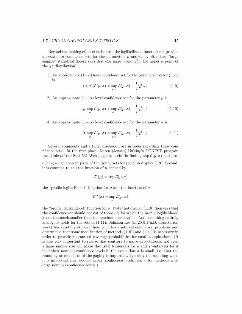
Beyond the making of point estimates, the loglikelihood function can provideapproximate con…dence sets for the parameters ¹ and/or ¾. Standard “largesample” statistical theory says that (for large n and Â2
®:º the upper ® point ofthe Â2
º distribution):
1. An approximate (1¡®) level con…dence set for the parameter vector (¹; ¾)is
f(¹; ¾)jL(¹; ¾) > sup¹;¾
L(¹; ¾) ¡ 12Â2
®:2g : (1.9)
2. An approximate (1 ¡ ®) level con…dence set for the parameter ¹ is
f¹j sup¾
L(¹; ¾) > sup¹;¾
L(¹; ¾) ¡ 12Â2
®:1g : (1.10)
3. An approximate (1 ¡ ®) level con…dence set for the parameter ¾ is
f¾j sup¹
L(¹; ¾) > sup¹;¾
L(¹;¾) ¡ 12Â2
®:1g : (1.11)
Several comments and a fuller discussion are in order regarding these con-…dence sets. In the …rst place, Karen (Jensen) Hulting’s CONEST program(available o¤ the Stat 531 Web page) is useful in …nding sup
¹;¾L(¹; ¾) and pro-
ducing rough contour plots of the (joint) sets for (¹; ¾) in display (1.9). Second,it is common to call the function of ¹ de…ned by
L¤(¹) = sup¾
L(¹; ¾)
the “pro…le loglikelihood” function for ¹ and the function of ¾
L¤¤(¾) = sup¹
L(¹; ¾)
the “pro…le loglikelihood” function for ¾. Note that display (1.10) then says thatthe con…dence set should consist of those ¹’s for which the pro…le loglikelihoodis not too much smaller than the maximum achievable. And something entirelyanalogous holds for the sets in (1.11). Johnson Lee (in 2001 Ph.D. dissertationwork) has carefully studied these con…dence interval estimation problems anddetermined that some modi…cation of methods (1.10) and (1.11) is necessary inorder to provide guaranteed coverage probabilities for small sample sizes. (Itis also very important to realize that contrary to naive expectations, not evena large sample size will make the usual t-intervals for ¹ and Â2-intervals for ¾hold their nominal con…dence levels in the event that ¾ is small, i.e. that therounding or crudeness of the gaging is important. Ignoring the rounding whenit is important can produce actual con…dence levels near 0 for methods withlarge nominal con…dence levels.)

16 CHAPTER 1. MEASUREMENT AND STATISTICS
Table 1.2: ¢ for 0-Range Samples Based on Very Small n®
n :05 :10 :202 3:084 1:547 :7853 :776 :5624 :517
Intervals for a Normal Mean Based on Integer-Rounded Data
Speci…cally regarding the sets for ¹ in display (1.10), Lee (in work to appear inthe Journal of Quality Technology) has shown that one must replace the valueÂ2
®:1 with something larger in order to get small n actual con…dence levels nottoo far from nominal for “most” (¹; ¾). In fact, the choice
c(n;®) = n ln
Ãt2®
2 :(n¡1)
n ¡ 1+ 1
!
(for t®2 :(n¡1) the upper ®
2 point of the t distribution with º = n ¡ 1 degrees offreedom) is appropriate.
After replacing Â2®:1 with c(n; ®) in display (1.10) there remains the numer-
ical analysis problem of actually …nding the interval prescribed by the display.The nature of the numerical analysis required depends upon the sample rangeencountered in the crudely gaged data. Provided the range is at least 2, L¤(¹)is well-behaved (continuous and “mound-shaped”) and even simple trial anderror with Karen (Jensen) Hulting’s CONEST program will quickly producethe necessary interval. When the range is 0 or 1, L¤(¹) has respectively 2 or 1discontinuities and the numerical analysis is a bit trickier. Lee has recorded theresults of the numerical analysis for small sample sizes and ® = :05; :10 and :20(con…dence levels respectively 95%; 90% and 80%).
When a sample of size n produces range 0 with, say, all observations equalto x¤, the intuition that one ought to estimate ¹ 2 (x¤ ¡ :5; x¤ + :5) is soundunless n is very small. If n and ® are as recorded in Table 1.2 then display(1.10) (modi…ed by the use of c(n; ®) in place of Â2
®:1) leads to the interval(x¤ ¡ ¢; x¤ + ¢). (Otherwise it leads to (x¤ ¡ :5; x¤ + :5) for these ®.)
In the case that a sample of size n produces range 1 with, say, all observationsx¤ or x¤ +1, the interval prescribed by display (1.10) (with c(n;®) used in placeof Â2
®:1) can be thought of as having the form (x¤ + :5¡¢L; x¤ + :5+¢U ) where¢L and ¢U depend upon
nx¤ = #[observations x¤] and nx¤+1 = #[observations x¤ + 1] . (1.12)
When nx¤ ¸ nx¤+1, it is the case that ¢L ¸ ¢U . And when nx¤ · nx¤+1,correspondingly ¢L · ¢U . Let
m = maxfnx¤ ; nx¤+1g (1.13)

1.7. CRUDE GAGING AND STATISTICS 17
Table 1.3: (¢1;¢2) for Range 1 Samples Based on Small n®
n m :05 :10 :202 1 (6:147; 6:147) (3:053; 3:053) (1:485; 1:485)3 2 (1:552; 1:219) (1:104; 0:771) (0:765; 0:433)4 3 (1:025; 0:526) (0:082; 0:323) (0:639; 0:149)
2 (0:880; 0:880) (0:646; 0:646) (0:441; 0:441)5 4 (0:853; 0:257) (0:721; 0:132) (0:592; 0:024)
3 (0:748; 0:548) (0:592; 0:339) (0:443; 0:248)6 5 (0:772; 0:116) (0:673; 0:032) (0:569; 0:000)
4 (0:680; 0:349) (0:562; 0:235) (0:444; 0:126)3 (0:543; 0:543) (0:420; 0:420) (0:299; 0:299)
7 6 (0:726; 0:035) (0:645; 0:000) (0:556; 0:000)5 (0:640; 0:218) (0:545; 0:130) (0:446; 0:046)4 (0:534; 0:393) (0:432; 0:293) (0:329; 0:193)
8 7 (0:698; 0:000) (0:626; 0:000) (0:547; 0:000)6 (0:616; 0:129) (0:534; 0:058) (0:446; 0:000)5 (0:527; 0:281) (0:439; 0:197) (0:347; 0:113)4 (0:416; 0:416) (0:327; 0:327) (0:236; 0:236)
9 8 (0:677; 0:000) (0:613; 0:000) (0:541; 0:000)7 (0:599; 0:065) (0:526; 0:010) (0:448; 0:000)6 (0:521; 0:196) (0:443; 0:124) (0:361; 0:054)5 (0:429; 0:321) (0:350; 0:242) (0:267; 0:163)
10 9 (0:662; 0:000) (0:604; 0:000) (0:537; 0:000)8 (0:587; 0:020) (0:521; 0:000) (0:450; 0:000)7 (0:515; 0:129) (0:446; 0:069) (0:371; 0:012)6 (0:437; 0:242) (0:365; 0:174) (0:289; 0:105)5 (0:346; 0:346) (0:275; 0:275) (0:200; 0:200)
and correspondingly take
¢1 = maxf¢L;¢Ug and ¢2 = minf¢L;¢Ug .
Table 1.3 then gives values for ¢1 and ¢2 for n · 10 and ® = :05; :10 and :2.
Intervals for a Normal Standard Deviation Based on Integer-RoundedData
Speci…cally regarding the sets for ¾ in display (1.11), Lee found that in orderto get small n actual con…dence levels not too far from nominal, one must notonly replace the value Â2
®:1 with something larger, but must make an additionaladjustment for samples with ranges 0 and 1.
Consider …rst replacing Â2®:1 in display (1.11) with a (larger) value d(n; ®)
given in Table 1.4. Lee found that for those (¹; ¾) with moderate to large ¾,

18 CHAPTER 1. MEASUREMENT AND STATISTICS
Table 1.4: d(n; ®) for Use in Estimating ¾®
n :05 :102 10:47 7:713 7:26 5:234 6:15 4:395 5:58 3:976 5:24 3:717 5:01 3:548 4:84 3:429 4:72 3:33
10 4:62 3:2615 4:34 3:0620 4:21 2:9730 4:08 2:881 3:84 2:71
making this d(n; ®) for Â2®:1 substitution is enough to produce an actual con-
…dence level approximating the nominal one. However, even this modi…cationis not adequate to produce an acceptable coverage probability for (¹;¾) withsmall ¾.
For samples with range 0 or 1, formula (1.11) prescribes intervals of the form(0; U). And reasoning that when ¾ is small, samples will typically have range0 or 1, Lee was able to …nd (larger) replacements for the limit U prescribed by(1.11) so that the resulting estimation method has actual con…dence level notmuch below the nominal level for any (¹; ¾) (with ¾ large or small).
That is if a 0-range sample is observed, estimate ¾ by
(0;¤0)
where ¤0 is taken from Table 1.5. If a range 1 sample is observed consisting,say, of values x¤ and x¤ +1, and nx¤ ; nx¤+1 and m are as in displays (1.12) and(1.13), estimate ¾ using
(0;¤1;m)
where ¤1;m is taken from Table 1.6.The use of these values ¤0 for range 0 samples, and ¤1;m for range 1 samples,
and the values d(n; ®) in place of Â2®:1 in display (1.11) …nally produces a reliable
method of con…dence interval estimation for ¾ when normal data are integer-rounded.
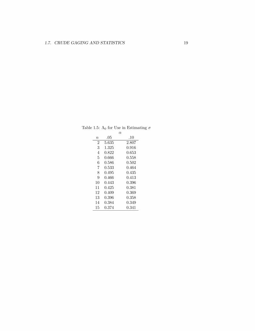
1.7. CRUDE GAGING AND STATISTICS 19
Table 1.5: ¤0 for Use in Estimating ¾®
n :05 :102 5:635 2:8073 1:325 0:9164 0:822 0:6535 0:666 0:5586 0:586 0:5027 0:533 0:4648 0:495 0:4359 0:466 0:413
10 0:443 0:39611 0:425 0:38112 0:409 0:36913 0:396 0:35814 0:384 0:34915 0:374 0:341

20 CHAPTER 1. MEASUREMENT AND STATISTICS
Table 1.6: ¤1;m for Use in Estimating ¾ (m in Parentheses)®
n :05 :102 16:914(1) 8:439(1)3 3:535(2) 2:462(2)4 1:699(3) 2:034(2) 1:303(3) 1:571(2)5 1:143(4) 1:516(3) 0:921(4) 1:231(3)6 0:897(5) 1:153(4) 1:285(3) 0:752(5) 0:960(4) 1:054(3)7 0:768(6) 0:944(5) 1:106(4) 0:660(6) 0:800(5) 0:949(4)8 0:687(7) 0:819(6) 0:952(5) 0:599(7) 0:707(6) 0:825(5)
1:009(4) 0:880(4)9 0:629(8) 0:736(7) 0:837(6) 0:555(8) 0:644(7) 0:726(6)
0:941(5) 0:831(5)10 0:585(9) 0:677(8) 0:747(7) 0:520(9) 0:597(8) 0:654(7)
0:851(6) 0:890(5) 0:753(6) 0:793(5)11 0:550(10) 0:630(9) 0:690(8) 0:493(10) 0:560(9) 0:609(8)
0:775(7) 0:851(6) 0:685(7) 0:763(6)12 0:522(11) 0:593(10) 0:646(9) 0:470(11) 0:531(10) 0:573(9)
0:708(8) 0:789(7) 0:818(6) 0:626(8) 0:707(7) 0:738(6)13 0:499(12) 0:563(11) 0:610(10) 0:452(12) 0:506(11) 0:544(10)
0:658(9) 0:733(8) 0:791(7) 0:587(9) 0:655(8) 0:716(7)14 0:479(13) 0:537(12) 0:580(11) 0:436(13) 0:485(12) 0:520(11)
0:622(10) 0:681(9) 0:745(8) 0:558(10) 0:607(9) 0:674(8)0:768(7) 0:698(7)
15 0:463(14) 0:515(13) 0:555(12) 0:422(14) 0:468(13) 0:499(12)0:593(11) 0:639(10) 0:701(9) 0:534(11) 0:574(10) 0:632(9)0:748(8) 0:682(8)

Chapter 2
Process Monitoring
Chapters 3 and 4 of V&J discuss methods for process monitoring. The keyconcept there regarding the probabilistic description of monitoring schemes isthe run length idea introduced on page 91 and speci…cally in display (3.44).Theory for describing run lengths is given in V&J only for the very simplest caseof geometrically distributed T . This chapter presents some more general toolsfor the analysis/comparison of run length distributions of monitoring schemes,namely discrete time …nite state Markov chains and recursions expressed interms of integral (and di¤erence) equations.
2.1 Some Theory for Stationary Discrete TimeFinite State Markov Chains With a SingleAbsorbing State
These are probability models for random systems that at times t = 1; 2; 3 : : :can be in one of a …nite number of states
S1;S2; : : : ;Sm;Sm+1 :
The “Markov” assumption is that the conditional distribution of where thesystem is at time t + 1 given the entire history of where it has been up throughtime t only depends upon where it is at time t. (In colloquial terms: Theconditional distribution of where I’ll be tomorrow given where I am and how I gothere depends only on where I am, not on how I got here.) So called “stationary”Markov Chain (MC) models employ the assumption that movement betweenstates from any time t to time t + 1 is governed by a (single) matrix of (one-step) “transition probabilities” (that is independent of t)
P(m+1)£(m+1)
= (pij)
where
pij = P [system is in Sj at time t + 1 j system is in Si at time t] :
21

22 CHAPTER 2. PROCESS MONITORING
S S
S
1 2
3
.1 .05
.8 .05
1.0
.1
.9
Figure 2.1: Schematic for a MC with Transition Matrix (2.1)
As a simple example of this, consider the transition matrix
P3£3
:=
0@
:8 :1 :1:9 :05 :050 0 1
1A : (2.1)
Figure 2.1 is a useful schematic representation of this model.The Markov Chain represented by Figure 2.1 has an interesting property.
That is, while it is possible to move back and forth between states 1 and 2,once the system enters state 3, it is “stuck” there. The standard jargon for thisproperty is to say that S3 is an absorbing state. (In general, if pii = 1, Si iscalled an absorbing state.)
Of particular interest in applications of MCs to the description of processmonitoring schemes are chains with a single absorbing state, say Sm+1, where itis possible to move (at least eventually) from any other state to the absorbingstate. One thing that makes these chains so useful is that it is very easy towrite down a matrix formula for a vector giving the mean number of transitionsrequired to reach Sm+1 from any of the other states. That is, with
Li = the mean number of transitions required to move from Si to Sm+1 ;
Lm£1
=
0BBB@
L1L2...
Lm
1CCCA ; P
(m+1)£(m+1)=
0@
Rm£m
rm£1
01£m
11£1
1A ; and 1
m£1=
0BBB@
11...1
1CCCA
it is the case thatL = (I ¡ R)¡11 : (2.2)

2.1. SOME THEORY FOR STATIONARY DISCRETE TIME FINITE STATE MARKOV CHAINS WITH A SIN
To argue that display (2.2) is correct, note that the following system of mequations “clearly” holds:
L1 = (1 + L1)p11 + (1 + L2)p12 + ¢ ¢ ¢ + (1 + Lm)p1m + 1 ¢ p1;m+1
L2 = (1 + L1)p21 + (1 + L2)p22 + ¢ ¢ ¢ + (1 + Lm)p2m + 1 ¢ p2;m+1
...Lm = (1 + L1)pm1 + (1 + L2)pm2 + ¢ ¢ ¢ + (1 + Lm)pmm + 1 ¢ pm;m+1 :
But this set is equivalent to the set
L1 = 1 + p11L1 + p12L2 + ¢ ¢ ¢ + p1mLm
L2 = 1 + p21L1 + p22L2 + ¢ ¢ ¢ + p2mLm
...Lm = 1 + pm1L1 + pm2L2 + ¢ ¢ ¢ + pmmLm
and in matrix notation, this second set of equations is
L = 1 + RL : (2.3)
SoL ¡ RL = 1 ;
i.e.(I ¡ R)L = 1 :
Under the conditions of the present discussion it is the case that (I ¡ R) isguaranteed to be nonsingular, so that multiplying both sides of this matrixequation by the inverse of (I ¡ R) one …nally has equation (2.2).
For the simple 3-state example with transition matrix (2.1) it is easy enoughto verify that with
R =µ
:8 :1:9 :05
¶
one has(I ¡ R)¡11 =
µ10:511
¶:
That is, the mean number of transitions required for absorption (into S3) fromS1 is 10:5 while the mean number required from S2 is 11:0.
When one is working with numerical values in P and thus wants numericalvalues in L, the matrix formula (2.2) is most convenient for use with numericalanalysis software. When, on the other hand, one has some algebraic expressionsfor the pij and wants algebraic expressions for the Li, it is usually most e¤ectiveto write out the system of equations represented by display (2.3) and to try andsee some slick way of solving for an Li of interest.
It is also worth noting that while the discussion in this section has centeredon the computation of mean times to absorption, other properties of “time toabsorption” variables can be derived and expressed in matrix notation. Forexample, Problem 2.22 shows that it is fairly easy to …nd the variance (orstandard deviation) of time to absorption variables.
24 CHAPTER 2. PROCESS MONITORING
2.2 Some Applications of Markov Chains to theAnalysis of Process Monitoring Schemes
When the “current condition” of a process monitoring scheme can be thoughtof as discrete random variable (with a …nite number of possible values), because
1. the variables Q1; Q2; ::. fed into it are intrinsically discrete (for examplerepresenting counts) and are therefore naturally modeled using a discreteprobability distribution (and the calculations prescribed by the schemeproduce only a …xed number of possible outcomes),
2. “discretization” of the Q’s has taken place as a part of the developmentof the monitoring scheme (as, for example, in the “zone test” schemesoutlined in Tables 3.5 through 3.7 of V&J), or
3. one approximates continuous distributions for Q’s and/or states of thescheme with a “…nely-discretized” version in order to approximate exact(continuous) run length properties,
one can often apply the material of the previous section to the prediction ofscheme behavior. (This is possible when the evolution of the monitoring schemecan be thought of in terms of movement between “states” where the conditionaldistribution of the next “state” depends only on a distribution for the next Qwhich itself depends only on the current “state” of the scheme.) This sectioncontains four examples of what can be done in this direction.
As an initial simple example, consider the simple monitoring scheme (sug-gested in the book Sampling Inspection and Quality Control by Wetherill) thatsignals an alarm the …rst time
1. a single point Q plots “outside 3 sigma limits,” or
2. two consecutive Q’s plot “between 2 and 3 sigma limits.”
(This is a simple competitor to the sets of alarm rules speci…ed in Tables 3.5through 3.7 of V&J.) Suppose that one assumes that Q1; Q2; : : : are iid and
q1 = P [Q1 plots outside 3 sigma limits]
andq2 = P [Q1 plots between 2 and 3 sigma limits] :
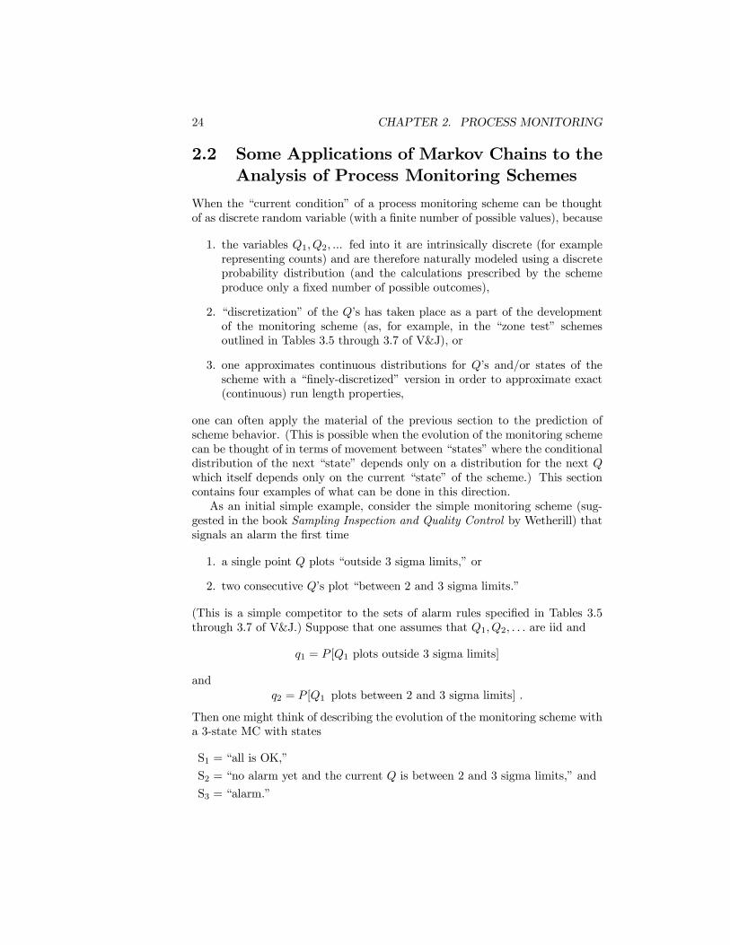
Then one might think of describing the evolution of the monitoring scheme witha 3-state MC with states
S1 = “all is OK,”S2 = “no alarm yet and the current Q is between 2 and 3 sigma limits,” andS3 = “alarm.”

2.2. SOME APPLICATIONS OF MARKOV CHAINS TO THE ANALYSIS OF PROCESS MONITORING SCH
q + q1 2
S3
S2S1
1- q - q1 2
q2
1- q - q1 2
q1
1.0
0
Figure 2.2: Schematic for a MC with Transition Matrix (2.4)
For this representation, an appropriate transition matrix is
P =
0@
1 ¡ q1 ¡ q2 q2 q11 ¡ q1 ¡ q2 0 q1 + q2
0 0 1
1A (2.4)
and the ARL of the scheme (under the iid model for the Q sequence) is L1, themean time to absorption into the alarm state from the “all-OK” state. Figure2.2 is a schematic representation of this scenario.
It is worth noting that a system of equations for L1 and L2 is
L1 = 1 ¢ q1 + (1 + L2)q2 + (1 + L1)(1 ¡ q1 ¡ q2)L2 = 1 ¢ (q1 + q2) + (1 + L1)(1 ¡ q1 ¡ q2) ;
which is equivalent to
L1 = 1 + L1 ¢ (1 ¡ q1 ¡ q2) + L2q2
L2 = 1 + L1(1 ¡ q1 ¡ q2) ;
which is the “non-matrix version” of the system (2.3) for this example. It iseasy enough to verify that this system of two linear equations in the unknownsL1 and L2 has a (simultaneous) solution with
L1 =1 + q2
1 ¡ (1 ¡ q1 ¡ q2) ¡ q2(1 ¡ q1 ¡ q2):
As a second application of MC technology to the analysis of a process moni-toring scheme, we will consider a so-called “Run-Sum” scheme. To de…ne such a

26 CHAPTER 2. PROCESS MONITORING
scheme, one begins with “zones” for the variable Q as indicated in Figure 3.9 ofV&J. Then “scores” are de…ned for various possible values of Q. For j = 0; 1; 2a score of +j is assigned to the eventuality that Q is in the “positive j-sigma to(j + 1)-sigma zone,” while a score of ¡j is assigned to the eventuality that Qis in the “negative j-sigma to (j + 1)-sigma zone.” A score of +3 is assigned toany Q above the “upper 3-sigma limit” while a score of ¡3 is assigned to any Qbelow the “lower 3-sigma limit.” Then, for the variables Q1; Q2; : : : one de…nescorresponding scores Q¤
1; Q¤2; : : : and “run sums” R1; R2; : : : where
Ri = “the ‘sum’ of scores Q¤ through time i under the provision that anew sum is begun whenever a score is observed with a sign di¤erentfrom the existing Run-Sum.”
(Note, for example, that a new score of Q¤ = +0 will reset a current Run-Sumof R = ¡2 to +0.) The Run-Sum scheme then signals at the …rst i for whichjQ¤
i j = 3 or jRij ¸ 4.Then de…ne states for a Run-Sum process monitoring scheme
S1 = “no alarm yet and R = ¡0,”S2 = “no alarm yet and R = ¡1,”S3 = “no alarm yet and R = ¡2,”S4 = “no alarm yet and R = ¡3,”S5 = “no alarm yet and R = +0,”S6 = “no alarm yet and R = +1,”S7 = “no alarm yet and R = +2,”S8 = “no alarm yet and R = +3,” andS9 = “alarm.”
If one assumes that the observations Q1; Q2; : : : are iid and for j = ¡3;¡2;¡1;¡0;+0;+1;+2;+3 lets
qj = P [Q¤1 = j] ;
an appropriate transition matrix for describing the evolution of the scheme is
P =
0BBBBBBBBBBBB@
q¡0 q¡1 q¡2 0 q+0 q+1 q+2 0 q¡3 + q+30 q¡0 q¡1 q¡2 q+0 q+1 q+2 0 q¡3 + q+30 0 q¡0 q¡1 q+0 q+1 q+2 0 q¡3 + q¡2 + q+30 0 0 q¡0 q+0 q+1 q+2 0 q¡3 + q¡2 + q¡1 + q+1
q¡0 q¡1 q¡2 0 q+0 q+1 q+2 0 q¡3 + q+3q¡0 q¡1 q¡2 0 0 q+0 q+1 q+2 q¡3 + q+3q¡0 q¡1 q¡2 0 0 0 q+0 q+1 q¡3 + q+2 + q+3q¡0 q¡1 q¡2 0 0 0 0 q+0 q¡3 + q+1 + q+2 + q+30 0 0 0 0 0 0 0 1
1CCCCCCCCCCCCA
and the ARL for the scheme is L1 = L5. (The fact that the 1st and 5th rows ofP are identical makes it clear that the mean times to absorption from S1 and S5

2.2. SOME APPLICATIONS OF MARKOV CHAINS TO THE ANALYSIS OF PROCESS MONITORING SCH
q-1
q0
q1
q2
qm
qm-1
q-m
h-h 0 2h/m-h/m h/m
f *(y)
... ...
Figure 2.3: Notational Conventions for Probabilities from Rounding Q ¡ k1Values
must be the same.) It turns out that clever manipulation with the “non-matrix”version of display (2.3) in this example even produces a fairly simple expressionfor the scheme’s ARL. (See Problem 2.24 and Reynolds (1971 JQT ) and thereferences therein in this …nal regard.)
To turn to a di¤erent type of application of the MC technology, considerthe analysis of a high side decision interval CUSUM scheme as described in§4.2 of V&J. Suppose that the variables Q1; Q2; : : : are iid with a continuousdistribution speci…ed by the probability density f(y). Then the variables Q1 ¡k1; Q2 ¡k1; Q3 ¡k1; : : : are iid with probability density f¤(y) = f(y+k1). For apositive integer m, we will think of replacing the variables Qi ¡k1 with versionsof them rounded to the nearest multiple of h=m before CUSUMing. Then theCUSUM scheme can be thought of in terms of a MC with states
Si = “no alarm yet and the current CUSUM is (i ¡ 1)µ
hm
¶”
for i = 1; 2; : : : ;m andSm+1 = “alarm.”
Then let
q¡m =Z ¡h+ 1
2( hm)
¡1f¤(y)dy = P [Q1 ¡ k1 · ¡h +
12
µhm
¶] ;
qm =Z 1
h¡12 ( h
m)f¤(y)dy = P [h ¡ 1
2
µhm
¶< Q1 ¡ k1] ;
and for ¡m < j < m take
qj =Z j( h
m)+ 12( h
m)
j( hm)¡ 1
2( hm)
f¤(y)dy : (2.5)
These notational conventions for probabilities q¡m; : : : ; qm are illustrated inFigure 2.3.
In this notation, the evolution of the high side decision interval CUSUMscheme can then be described in approximate terms by a MC with transition

28 CHAPTER 2. PROCESS MONITORING
matrix
P(m+1)£(m+1)
=
0BBBBBBBBBBBBBBBBBBBB@
0X
j=¡m
qj q1 q2 ¢ ¢ ¢ qm¡1 qm
¡1X
j=¡m
qj q0 q1 ¢ ¢ ¢ qm¡2 qm¡1 + qm
¡2X
j=¡m
qj q¡1 q0 ¢ ¢ ¢ qm¡3 qm¡2 + qm¡1 + qm
......
......
...
q¡m + q¡m+1 q¡m+2 q¡m+3 ¢ ¢ ¢ q0
mX
j=1
qj
0 0 0 ¢ ¢ ¢ 0 1
1CCCCCCCCCCCCCCCCCCCCA
:
For i = 1; : : : ;m the mean time to absorption from state Si (Li) is approximatelythe ARL of the scheme with head start (i ¡ 1)
¡ hm
¢. (That is, the entries of the
vector L speci…ed in display (2.2) are approximate ARL values for the CUSUMscheme using various possible head starts.) In practice, in order to …nd ARLsfor the original scheme with non-rounded iid observations Q, one would …ndapproximate ARL values for an increasing sequence of m’s until those appearto converge for the head start of interest.
As a …nal example of the use of MC techniques in the probability modelingof process monitoring scheme behavior, consider discrete approximation of theEWMA schemes of §4.1 of V&J where the variables Q1; Q2; : : : are again iidwith continuous distribution speci…ed by a pdf f(y). In this case, in order toprovide a tractable discrete approximation, it will not typically su¢ce to simplydiscretize the variables Q (as the EWMA calculations will then typically producea number of possible/exact EWMA values that grows as time goes on). Instead,it is necessary to think directly in terms of rounded/discretized EWMAs. So foran odd positive integer m, let ¢ = (UCLEWMA ¡LCLEWMA)=m and think ofreplacing an (exact) EWMA sequence with a rounded EWMA sequence takingon values ai de…ned by
ai:= LCLEWMA +
¢2
+ (i ¡ 1)¢
for i = 1; 2; : : : ;m. For i = 1; 2; :::;m let
Si = “no alarm yet and the rounded EWMA is ai”
and
Sm+1 = “alarm.”

2.3. INTEGRAL EQUATIONS AND RUN LENGTH PROPERTIES OF PROCESS MONITORING SCHEMES2
And for 1 · i; j · m, let
qij = P [moving from Si to Sj ] ;
= P [aj ¡ ¢2
· (1 ¡ ¸)ai + ¸Q · aj +¢2
] ;
= P [aj ¡ (1 ¡ ¸)ai
¸¡ ¢
2¸· Q · aj ¡ (1 ¡ ¸)ai
¸+
¢2¸
] ;
= P [ai +(j ¡ i)¢
¸¡ ¢
2¸· Q · ai +
(j ¡ i)¢¸
+¢2¸
] ;
=Z ai+
(j¡i)¢¸ + ¢
2¸
ai+(j¡i)¢
¸ ¡ ¢2¸
f(y)dy : (2.6)
Then with
P =
0BBBBBBBBBBBBBB@
q11 q12 ¢ ¢ ¢ q1m 1 ¡mX
j=1
q1j
q21 q22 ¢ ¢ ¢ q2m 1 ¡mX
j=1
q2j
......
......
qm1 qm2 ¢ ¢ ¢ qmm 1 ¡mX
j=1
qmj
0 0 ¢ ¢ ¢ 0 1
1CCCCCCCCCCCCCCA
the mean time to absorption from the state S(m+1)=2 (the value L(m+1)=2) ofa MC with this transition matrix is an approximation for the EWMA schemeARL with EWMA0 = (UCLEWMA + LCLEWMA)=2. In practice, in order to…nd the ARL for the original scheme, one would …nd approximate ARL valuesfor an increasing sequence of m’s until those appear to converge.
The four examples in this section have illustrated the use of MC calculationsin the second and third of the two circumstances listed at the beginning of thissection. The …rst circumstance is conceptually the simplest of the three, and isfor example illustrated by Problems 2.25, 2.28 and 2.37. The examples have alsoall dealt with iid models for the Q1; Q2; : : : sequence. Problem 2.26 shows thatthe methodology can also easily accommodate some kinds of dependencies inthe Q sequence. (The discrete model in Problem 2.26 is itself perhaps less thancompletely appealing, but the reader should consider the possibility of discreteapproximation of the kind of dependency structure employed in Problem 2.27before dismissing the basic concept illustrated in Problem 2.26 as useless.)
2.3 Integral Equations and Run Length Proper-ties of Process Monitoring Schemes
There is a second (and at …rst appearance quite di¤erent) standard method ofapproaching the analysis of the run length behavior of some process monitoring

30 CHAPTER 2. PROCESS MONITORING
schemes where continuous variables Q are involved. That is through the use ofintegral equations, and this section introduces the use of these. (As it turns out,by the time one is forced to …nd numerical solutions of the integral equations,there is not a whole lot of di¤erence between the methods of this section andthose of the previous one. But it is important to introduce this second point ofview and note the correspondence between approaches.)
Before going to the details of speci…c schemes and integral equations, a smallpiece of calculus/numerical analysis needs to be reviewed and notation set foruse in these notes. That concerns the approximation of de…nite integrals on theinterval [a; a + h]. Speci…cation of a set of points
a · a1 · a2 · ¢ ¢ ¢ · am · a + h
and weights
wi ¸ 0 withmX
i=1
wi = h
so that Z a+h
af(y)dy may be approximated as
mX
i=1
wif(ai)
for “reasonable” functions f(y), is the speci…cation of a so-called “quadraturerule” for approximating integrals on the interval [a; a+h]. The simplest of suchrules is probably the choice
ai:= a +
µi ¡ 1
2m
¶h with wi
:=hm
: (2.7)
(This choice amounts to approximating an integral of f by a sum of signed areasof rectangles with bases h=m and (signed) heights chosen as the values of f atmidpoints of intervals of length h=m beginning at a.)
Now consider a high side CUSUM scheme as in §4.2 of V&J, where Q1; Q2; : : :are iid with continuous marginal distribution speci…ed by the probability densityf(y). De…ne the function
L1(u) := the ARL of the high side CUSUM scheme using a head start of u :
If one begins CUSUMing at u, there are three possibilities of where he/she will beafter a single observation, Q1. If Q1 is large (Q1 ¡k1 ¸ h¡u) then there will bean immediate signal and the run length will be 1. If Q1 is small (Q1 ¡k1 · ¡u)the CUSUM will “zero out,” one observation will have been “spent,” and onaverage L1(0) more observations are to be faced in order to produce a signal.Finally, if Q1 is moderate (¡u < Q1 ¡ k1 < h ¡ u) then one observation willhave been spent and the CUSUM will continue from u+(Q1 ¡k1), requiring onaverage an additional L1(u + (Q1 ¡ k1)) observations to produce a signal. Thisreasoning leads to the equation for L1,
L1(u) = 1 ¢ P [Q1 ¡ k1 ¸ h ¡ u] + (1 + L1(0))P [Q1 ¡ k1 · ¡u]
+Z k1+h¡u
k1¡u(1 + L1(u + y ¡ k1))f(y)dy :

2.3. INTEGRAL EQUATIONS AND RUN LENGTH PROPERTIES OF PROCESS MONITORING SCHEMES3
Writing F (y) for the cdf of Q1 and simplifying slightly, this is
L1(u) = 1 + L1(0)F (k1 ¡ u) +Z h
0L1(y)f(y + k1 ¡ u)dy : (2.8)
The argument leading to equation (2.8) has a twin that produces an integralequation for
L2(v) := the ARL of a low side CUSUM scheme using a head start of v :
That equation is
L2(v) = 1 + L2(0) (1 ¡ F (k2 ¡ u)) +Z 0
¡hL2(y)f(y + k2 ¡ v)dy : (2.9)
And as indicated in display (4.20) of V&J, could one solve equations (2.8) and(2.9) (and thus obtain L1(0) and L2(0)) one would have not only separate highand low side CUSUM ARLs, but ARLs for some combined schemes as well.(Actually, more than what is stated in V&J can be proved. Yashchin in aJournal of Applied Probability paper in about 1985 showed that with iid Q’s,high side decision interval h1 and low side decision interval ¡h2 for nonnegativeh2, if k1 ¸ k2 and
(k1 ¡ k2) ¡ jh1 ¡ h1j ¸ max (0; u ¡ v ¡ max(h1; h2)) ;
for the simultaneous use of high and low side schemes
ARLcombined =L1(0)L2(v) + L1(u)L2(0) ¡ L1(0)L2(0)
L1(0) + L2(0):
It is easily veri…ed that what is stated on page 151 of V&J is a special case ofthis result.) So in theory, to …nd ARLs for CUSUM schemes one need “only”solve the integral equations (2.8) and (2.9). This is easier said than done. Theone case where fairly explicit solutions are known is that where observations areexponentially distributed (see Problem 2.30). In other cases one must resort tonumerical solution of the integral equations.
So consider the problem of approximate solution of equation (2.8). Fora particular quadrature rule for integrals on [0; h], for each ai one has fromequation (2.8) the approximation
L1(ai) ¼ 1 + L1(a1)F (k1 ¡ ai) +mX
j=1
wjL1(aj)f(aj + k1 ¡ ai) :
32 CHAPTER 2. PROCESS MONITORING
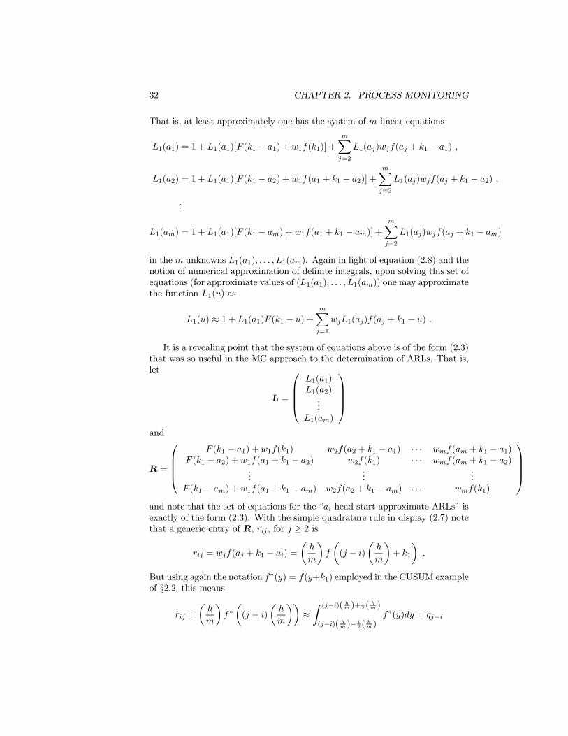
That is, at least approximately one has the system of m linear equations
L1(a1) = 1 + L1(a1)[F (k1 ¡ a1) + w1f(k1)] +mX
j=2
L1(aj)wjf(aj + k1 ¡ a1) ;
L1(a2) = 1 + L1(a1)[F (k1 ¡ a2) + w1f(a1 + k1 ¡ a2)] +mX
j=2
L1(aj)wjf(aj + k1 ¡ a2) ;
...
L1(am) = 1 + L1(a1)[F (k1 ¡ am) + w1f(a1 + k1 ¡ am)] +mX
j=2
L1(aj)wjf(aj + k1 ¡ am)
in the m unknowns L1(a1); : : : ; L1(am). Again in light of equation (2.8) and thenotion of numerical approximation of de…nite integrals, upon solving this set ofequations (for approximate values of (L1(a1); : : : ; L1(am)) one may approximatethe function L1(u) as
L1(u) ¼ 1 + L1(a1)F (k1 ¡ u) +mX
j=1
wjL1(aj)f(aj + k1 ¡ u) :
It is a revealing point that the system of equations above is of the form (2.3)that was so useful in the MC approach to the determination of ARLs. That is,let
L =
0BBB@
L1(a1)L1(a2)
...L1(am)
1CCCA
and
R =
0BBB@
F (k1 ¡ a1) + w1f(k1) w2f(a2 + k1 ¡ a1) ¢ ¢ ¢ wmf(am + k1 ¡ a1)F (k1 ¡ a2) + w1f(a1 + k1 ¡ a2) w2f(k1) ¢ ¢ ¢ wmf(am + k1 ¡ a2)
......
...F (k1 ¡ am) + w1f(a1 + k1 ¡ am) w2f(a2 + k1 ¡ am) ¢ ¢ ¢ wmf(k1)
1CCCA
and note that the set of equations for the “ai head start approximate ARLs” isexactly of the form (2.3). With the simple quadrature rule in display (2.7) notethat a generic entry of R; rij , for j ¸ 2 is
rij = wjf(aj + k1 ¡ ai) =µ
hm
¶f
µ(j ¡ i)
µhm
¶+ k1
¶:
But using again the notation f¤(y) = f(y+k1) employed in the CUSUM exampleof §2.2, this means
rij =µ
hm
¶f¤
µ(j ¡ i)
µhm
¶¶¼
Z (j¡i)( hm)+ 1
2( hm)
(j¡i)( hm)¡ 1
2( hm)
f¤(y)dy = qj¡i

2.3. INTEGRAL EQUATIONS AND RUN LENGTH PROPERTIES OF PROCESS MONITORING SCHEMES3
(in terms of the notation (2.5) from the CUSUM example). The point is thatwhether one begins from a “discretize the Q ¡ k1 distribution and employ theMC material” point of view or from a “do numerical solution of an integralequation” point of view is largely immaterial. Very similar large systems oflinear equations must be solved in order to …nd approximate ARLs.
As a second application of integral equation ideas to the analysis of processmonitoring schemes, consider the EWMA schemes of §4.1 of V&J where Q1; Q2; : : :are iid with a continuous distribution speci…ed by the probability density f(y).Let
L(u) = the ARL of a EWMA scheme with EWMA0 = u :
When one begins a EWMA sequence at u, there are 2 possibilities of wherehe/she will be after a single observation, Q1. If Q1 is extreme (¸Q1 +(1¡¸)u >UCLEWMA or ¸Q1 + (1 ¡ ¸)u < LCLEWMA) then there will be an immediatesignal and the run length will be 1. If Q1 is moderate (LCLEWMA · ¸Q1 +(1¡¸)u · UCLEWMA) one observation will have been “spent” and on averageL(¸Q1+(1¡¸)u) more observations are to be faced in order to produce a signal.Now the event
LCLEWMA · ¸Q1 + (1 ¡ ¸)u · UCLEWMA
is the event
LCLEWMA ¡ (1 ¡ ¸)u¸
· Q1 · UCLEWMA ¡ (1 ¡ ¸)u¸
;
so this reasoning produces the equation
L(u) = 1 ¢µ
1 ¡ P [LCLEWMA ¡ (1 ¡ ¸)u
¸· Q1 · UCLEWMA ¡ (1 ¡ ¸)u
¸]¶
+Z UCLEWMA¡(1¡¸)u
¸
LCLEWMA¡(1¡¸)u¸
(1 + L(¸y + (1 ¡ ¸)u)) f(y)dy ;
or
L(u) = 1 +Z UCLEWMA¡(1¡¸)u
¸
LCLEWMA¡(1¡¸)u¸
L(¸y + (1 ¡ ¸)u)f(y)dy ;
or …nally
L(u) = 1 +1¸
Z UCLEWMA
LCLEWMA
L(y)fµ
y ¡ (1 ¡ ¸)u¸
¶dy : (2.10)
As in the previous (CUSUM) case, one must usually resort to numericalmethods in order to approximate the solution to equation (2.10). For a partic-ular quadrature rule for integrals on [LCLEWMA; UCLEWMA], for each ai onehas from equation (2.10) the approximation
L(ai) ¼ 1 +1¸
mX
j=1
wjL(aj)fµ
aj ¡ (1 ¡ ¸)ai
¸
¶: (2.11)

34 CHAPTER 2. PROCESS MONITORING
Now expression (2.11) is standing for a set of m equations in the m unknownsL(a1); : : : ; L(am) that (as in the CUSUM case) can be thought of in terms ofthe matrix expression (2.3) if one takes
L =
0B@
L(a1)...
L(am)
1CA and R
m£m=
0@
wjf³
aj¡(1¡¸)ai¸
´
¸
1A : (2.12)
Solution of the system represented by equation (2.11) or the matrix expression(2.3) with de…nitions (2.12) produces approximate values for L(a1); : : : ; L(am)and therefore an approximation for the function L(u) as
L(u) ¼ 1 +1¸
mX
j=1
wjL(aj)fµ
aj ¡ (1 ¡ ¸)u¸
¶:
Again as in the CUSUM case, it is worth noting the similarity between theset of equations used to …nd “MC” ARL approximations and the set of equa-tions used to …nd “integral equation” ARL approximations. With the quadra-ture rule (2.7) and an odd integer m, using the notation ¢ = (UCLEWMA ¡LCLEWMA)=m employed in §2.2 in the EWMA example, note that a genericentry of R de…ned in (2.12) is
rij =wjf
³aj¡(1¡¸)ai
¸
´
¸=
¢f³ai + (j¡i)¢
¸
´
¸¼
Z ai+(j¡i)¢
¸ + ¢2¸
ai+(j¡i)¢
¸ ¡ ¢2¸
f(y)dy = qij ;
(in terms of the notation (2.6) from the EWMA example of §2.2). That is,as in the CUSUM case, the sets of equations used in the “MC” and “integralequation” approximations for the “EWMA0 = ai ARLs” of the scheme are verysimilar.
As a …nal example of the use of integral equations in the analysis of processmonitoring schemes, consider the X=MR schemes of §4.4 of V&J. Suppose thatobservations x1; x2; : : : are iid with continuous marginal distribution speci…edby the probability density f(y). De…ne the function
L(y) = “the mean number of additional observations to alarm, given thatthere has been no alarm to date and the current observation is y.”
Then note that as one begins X=MR monitoring, there are two possibilities ofwhere he/she will be after observing the …rst individual, x1. If x1 is extreme(x1 < LCLx or x1 > UCLx) there will be an immediate signal and the runlength will be 1. If x1is not extreme (LCLx · x1 · UCLx) one observationwill have been spent and on average another L(x1) observations will be requiredin order to produce a signal. So it is reasonable that the ARL for the X=MRscheme is
ARL = 1 ¢ (1 ¡ P [LCLx · x1 · UCLx]) +Z UCLx
LCLx
(1 + L(y))f(y)dy ;

2.3. INTEGRAL EQUATIONS AND RUN LENGTH PROPERTIES OF PROCESS MONITORING SCHEMES3
that is
ARL = 1 +Z UCLx
LCLx
L(y)f(y)dy ; (2.13)
where it remains to …nd a way of computing the function L(y) in order to feedit into expression (2.13).
In order to derive an integral equation for L(y) consider the situation if therehas been no alarm and the current individual observation is y. There are twopossibilities of where one will be after observing one more individual, x. If xis extreme or too far from y (x < LCLx or x > UCLx or jx ¡ yj > UCLR)only one additional observation is required to produce a signal. On the otherhand, if x is not extreme and not too far from y (LCLx · x · UCLx andjx ¡ yj · UCLR) one more observation will have been spent and on averageanother L(x) will be required to produce a signal. That is,
L(y) = 1 ¢ (P [x < LCLx or x > UCLx or jx ¡ yj > UCLR])
+Z min(UCLx;y+UCLR)
max(LCLx;y¡UCLR)(1 + L(x))f(x)dx ;
that is,
L(y) = 1 +Z min(UCLx;y+UCLR)
max(LCLx;y¡UCLR)L(x)f(x)dx
= 1 +Z UCLx
LCLx
I[jx ¡ yj · UCLR]L(x)f(x)dx : (2.14)
(The notation I[A] is “indicator function” notation, meaning that when A holdsI[A] = 1; and otherwise I[A] = 0.) As in the earlier CUSUM and EWMA ex-amples, once one speci…es a quadrature rule for de…nite integrals on the interval[LCLx; UCUx], this expression (2.14) provides a set of m linear equations forapproximate values of L(ai)’s. When this system is solved, the resulting valuescan be fed into a discretized version of equation (2.13) and an approximate ARLproduced. It is worth noting that the potential discontinuities of the integrandin equation (2.14) (produced by the indicator function) have the e¤ect of mak-ing numerical solutions of this equation much less well-behaved than those forthe other integral equations developed in this section.
The examples of this section have dealt only with ARLs for schemes basedon (continuous) iid observations. It therefore should be said that:
1. The iid assumption can in some cases be relaxed to give tractable integralequations for situations where correlated sequences Q1; Q2; : : : are involved(see for example Problem 2.27),
2. Other descriptors of the run length distribution (beyond the ARL) canoften be shown to solve simple integral equations (see for example theintegral equations for CUSUM run length second moment and run lengthprobability function in Problem 2.31), and

36 CHAPTER 2. PROCESS MONITORING
3. In some cases, with discrete variables Q there are di¤erence equation ana-logues of the integral equations presented here (that ultimately correspondto the kind of MC calculations illustrated in the previous section).

Chapter 3
An Introduction to DiscreteStochastic ControlTheory/Minimum VarianceControl
Section 3.6 of V&J provides an elementary introduction to the topic of Engi-neering Control and contrasts this adjustment methodology with (the processmonitoring methodology of) control charting. The last item under the En-gineering Control heading of Table 3.10 of V&J makes reference to “optimalstochastic control” theory. The object of this theory is to model system behav-ior using probability tools and let the consequences of the model assumptionshelp guide one in the choice of e¤ective control/adjustment algorithms. Thischapter provides a very brief introduction to this theory.
3.1 General ExpositionLet
f: : : ; Z(¡1); Z(0); Z(1); Z(2); : : :gstand for observations on a process assuming that no control actions are taken.One …rst needs a stochastic/probabilistic model for the sequence fZ(t)g, andwe will let
Fstand for such a model. F is a joint distribution for the Z’s and might, forexample, be:
1. a simple random walk model speci…ed by the equation Z(t) = Z(t ¡ 1) +²(t), where the ²’s are iid normal (0; ¾2) random variables,
37
38CHAPTER 3. AN INTRODUCTION TO DISCRETE STOCHASTIC CONTROL THEORY/MIN
2. a random walk model with drift speci…ed by the equation Z(t) = Z(t ¡1)+d+²(t), where d is a constant and the ²’s are iid normal (0; ¾2) randomvariables, or
3. some Box-Jenkins ARIMA model for the fZ(t)g sequence.
Then leta(t)
stand for a control action taken at time t, after observing the process. Oneneeds notation for the current impact of control actions taken in past periods,so we will further let
A(a; s)
stand for the current impact on the process of a control action a taken s periodsago. In many systems, the control actions, a, are numerical, and A(a; s) = ah(s)where h(s) is the so-called “impulse response function” giving the impact of aunit control action taken s periods previous. A(a; s) might, for example, be:
1. given by A(a; s) = a for s ¸ 1 in a machine tool control problem where “a”means “move the cutting tool out a units” (and the controlled variable isa measured dimension of a work piece),
2. given by A(a; s) = 0 for s · u and by A(a; s) = a for s > u in a machinetool control problem where “a” means “move the cutting tool out a units”and there are u periods of dead time, or
3. given by A(a; s) =¡1 ¡ exp
¡¡sh¿
¢¢a for s ¸ 1 in a chemical process
control problem with time constant ¿ and control period h seconds.
We will then assume that what one actually observes for (controlled) processbehavior at time t ¸ 1 is
Y (t) = Z(t) +t¡1X
s=0
A(a(s); t ¡ s) ;
which is the sum of what would have been observed with no control and all ofthe current e¤ects of previous control actions. For t ¸ 0, a(t) will be chosenbased on
f: : : ; Z(¡1); Z(0); Y (1); Y (2); : : : ; Y (t)g :
A common objective in this context is to choose the actions so as to minimize
EF (Y (t) ¡ T (t))2
ortX
s=1
EF (Y (s) ¡ T (s))2

3.1. GENERAL EXPOSITION 39
for some (possibly time-dependent) target value T (s). The problem of choosingof control actions to accomplish this goal is called the “minimum variance“(MV) control problem, and it has a solution that can be described in fairly(deceptively, perhaps) simple terms.
Note …rst that given f: : : ; Z(¡1); Z(0); Y (1); Y (2); : : : ; Y (t)g one can recoverf: : : ; Z(¡1); Z(0); Z(1); Z(2); : : : ; Z(t)g. This is because
Z(s) = Y (s) ¡s¡1X
r=0
A(a(r); s ¡ r)
i.e., to get Z(s), one simply subtracts the (known) e¤ects of previous controlactions from Y (s).
Then the model F (at least in theory) provides one a conditional distributionfor Z(t + 1); Z(t + 2); Z(t + 3); : : : given the observed Z’s through time t. Theconditional distribution for Z(t + 1); Z(t + 2); Z(t + 3) : : : given what one canobserve through time t, namely f: : : ; Z(¡1); Z(0); Y (1); Y (2); : : : ; Y (t)g, is thenthe conditional distribution one gets for Z(t+1); Z(t+2); Z(t+3); : : : from themodel F after recovering Z(1); Z(2); : : : ; Z(t) from the corresponding Y ’s. Thenfor s ¸ t + 1, let
EF [Z(s)j : : : ; Z(¡1); Z(0); Z(1); Z(2); : : : ; Z(t)] or just EF [Z(s)jZt]
stand for the mean of this conditional distribution of Z(s) available at time t.Suppose that there are u ¸ 0 periods of dead time (u could be 0). Then
the earliest Y that one can hope to in‡uence by choice of a(t) is Y (t + u + 1).Notice then that if one takes action a(t) at time t, one’s most natural projectionof Y (t + u + 1) at time t is
bY (t+u+1jt) := EF [Z(t +u+1)jZt] +t¡1X
s=0
A(a(s); t +u+1 ¡ s) +A(a(t); u+1)
It is then natural (and in fact turns out to give the MV control strategy) to tryto choose a(t) so that
bY (t + u + 1jt) = T (t + u + 1) :
That is, the MV strategy is to try to choose a(t) so that
A(a(t); u+1) = T (t+u+1)¡(
EF [Z(t + u + 1)jZt] +t¡1X
s=0
A(a(s); t + u + 1 ¡ s)
):
A caveat here is that in practice MV control tends to be “ragged.” Thatis, in order to exactly optimize the mean squared error, constant tweaking (andoften fairly large adjustments are required). By changing one’s control objectivesomewhat it is possible to produce “smoother” optimal control policies that are

40CHAPTER 3. AN INTRODUCTION TO DISCRETE STOCHASTIC CONTROL THEORY/MIN
nearly as e¤ective as MV algorithms in terms of keeping a process on target.That is, instead of trying to optimize
EF
tX
s=1
(Y (s) ¡ T (s))2 ;
in a situation where the a’s are numerical (a = 0 indicating “no adjustment”and the “size” of adjustments increasing with jaj) one might for a constant ¸ > 0set out to minimize the alternative criterion
EF
ÃtX
s=1
(Y (s) ¡ T (s))2 + ¸t¡1X
s=0
(a(s))2!
:
Doing so will “smooth” the MV algorithm.
3.2 An ExampleTo illustrate the meaning of the preceding formalism, consider the model (F)speci…ed by
Z(t) = W (t) + ²(t) for t ¸ 0and W (t) = W (t ¡ 1) + d + º(t) for t ¸ 1
¾(3.1)
for d a (known) constant, the ²’s normal (0; ¾2² ), the º’s normal (0; ¾2
º) andall the ²’s and º’s independent. (Z(t) is a random walk with drift observedwith error.) Under this model and an appropriate 0 mean normal initializingdistribution for W(0), it is the case that each
bZ(t + 1j t) := EF [Z(t + 1)jZ(0); : : : ; Z(t)]
may be computed recursively as
bZ(t + 1jt) = ®Z(t) + (1 ¡ ®) bZ(tjt ¡ 1) + d
for some constant ® (that depends upon the known variances ¾2² and ¾2
º).We will …nd MV control policies under model (3.1) with two di¤erent func-
tions A(a; s). Consider …rst the possibility
A(a; s) = a 8s ¸ 1 ; (3:2:2) (3.2)
(an adjustment “a” at a given time period takes its full and permanent e¤ectat the next time period).
Consider the situation at time t = 0. Available are Z(0) and bZ(0j¡1) (theprior mean of W (0)) and from these one may compute the prediction
bZ(1j0) := ®Z(0) + (1 ¡ ®) bZ(0j¡1) + d :

3.2. AN EXAMPLE 41
That means that taking control action a(0), one should predict a value of
bY (1j0) := bZ(1j0) + a(0)
for the controlled process at time t = 1, and upon setting this equal to thetarget T (1) and solving for a(0) one should thus choose
a(0) = T (1) ¡ bZ(1j0) :
At time t = 1 one has observed Y (1) and may recover Z(1) by noting that
Y (1) = Z(1) + A(a(0); 1) = Z(1) + a(0) ;
so thatZ(1) = Y (1) ¡ a(0) :
Then a prediction (of the uncontrolled process) one step ahead is
bZ(2j1) := ®Z(1) + (1 ¡ ®) bZ(1j0) + d :
That means that with a target of T (2) one should predict a value of the con-trolled process at time t = 2 of
bY (2j1) := bZ(2j1) + a(0) + a(1) :
Upon setting this value equal to T (2) and solving it is clear that one shouldchoose
a(1) = T (2) ¡³
bZ(2j1) + a(0)´
:
So in general under (3.2), at time t one may note that
Z(t) = Y (t) ¡t¡1X
s=0
a(s)
and (recursively) compute
bZ(t + 1jt) := ®Z(t) + (1 ¡ ®) bZ(tjt ¡ 1) + d :
Then setting the predicted value of the controlled process equal to T (t+1) andsolving for a(t), …nd the MV control action
a(t) = T (t + 1) ¡Ã
bZ(t + 1jt) +t¡1X
s=0
a(s)
!:
Finally, consider the problem of MV control under the same model (3.1),but now using
A(a; s) =½
0 if s = 1a for s = 2; 3; : : : (3.3)

42CHAPTER 3. AN INTRODUCTION TO DISCRETE STOCHASTIC CONTROL THEORY/MIN
(a description of response to process adjustment involving one period of delay,after which the full e¤ect of an adjustment is immediately and permanentlyfelt).
Consider the situation at time t = 0. In hand are Z(0) and the prior meanof W (0), bZ(0j¡1), and the …rst Y that one can a¤ect by choice of a(0) is Y (2).Now
Z(2) = W (2) + ²(2) ;= W (1) + d + º(2) + ²(2) ;= Z(1) ¡ ²(1) + d + º(2) + ²(2)
so that
bZ(2j0) := EF [Z(2)jZ(0)] ;= EF [Z(1) ¡ ²(1) + d + º(2) + ²(2)jZ(0)] ;
= bZ(1j0) + d ;
= ®Z(0) + (1 ¡ ®) bZ(0j¡1) + 2d
is a prediction of where the uncontrolled process will be at time t = 2. Then aprediction for the controlled process at time t = 2 is
bY (2j0) := bZ(2j0) + A(a(0); 2) = bZ(2j0) + a(0)
and upon setting this equal to the time t = 2 target, T (2), and solving, one hasthe MV control action
a(0) = T (2) ¡ bZ(2j0) :
At time t = 1 one has in hand Y (1) = Z(1) and bZ(1j0) and the …rst Y thatcan be a¤ected by the choice of a(1) is Y (3). Now
Z(3) = W (3) + ²(3) ;= W (2) + d + º(3) + ²(3) ;= Z(2) ¡ ²(2) + d + º(3) + ²(3)
so that
bZ(3j1) := EF [Z(3)jZ(0); Z(1)] ;= EF [Z(2) ¡ ²(2) + d + º(3) + ²(3)jZ(0); Z(1)] ;
= bZ(2j1) + d ;
= ®Z(1) + (1 ¡ ®) bZ(1j0) + 2d
is a prediction of where the uncontrolled process will be at time t = 3. Then aprediction for the controlled process at time t = 3 is
bY (3j1) := bZ(3j1) + A(a(0); 3) + A(a(1); 2) = bZ(3j1) + a(0) + a(1)

3.2. AN EXAMPLE 43
and upon setting this equal to the time t = 3 target, T (3), and solving, one hasthe MV control action
a(1) = T (3) ¡³
bZ(3j1) + a(0)´
:
Finally, in general under (3.3), one may at time t note that
Z(t) = Y (t) ¡t¡2X
s=0
a(s)
and (recursively) compute
bZ(t + 2jt) := ®Z(t) + (1 ¡ ®) bZ(tjt ¡ 1) + 2d :
Then setting the time t + 2 predicted value of the controlled process equal toT (t + 2) and solving for a(t), we …nd the MV control action
a(t) = T (t + 2) ¡Ã
bZ(t + 2jt) +t¡1X
s=0
a(s)
!:

44CHAPTER 3. AN INTRODUCTION TO DISCRETE STOCHASTIC CONTROL THEORY/MIN

Chapter 4
Process Characterizationand Capability Analysis
Sections 5.1 through 5.3 of V&J discuss the problem of summarizing the be-havior of a stable process. The “bottom line” of that discussion is that one-sample statistical methods can be used in a straightforward manner to char-acterize a process/population/universe standing behind data collected understable process conditions. Section 5.5 of V&J opens a discussion of summariz-ing process behavior when it is not sensible to model all data in hand as randomdraws from a single/…xed universe. The notes in this chapter carry the themeof §5.5 of V&J slightly further and add some theoretical detail missing in thebook.
4.1 General Comments on Assessing and Dis-secting “Overall Variation”
The questions “How much variation is there overall?” and “Where is the varia-tion coming from?” are fundamental to process characterization/understandingand the guidance of improvement e¤orts. To provide a framework for discus-sion here, suppose that in hand one has r samples of data, sample i of size ni(i = 1; : : : ; r). Depending upon the speci…c application, these r samples canhave many di¤erent logical structures. For example, §5.5 of V&J considers thecase where the ni are all the same and the r samples are naturally thought of ashaving a balanced hierarchical/tree structure. But many others (both “regular”and completely “irregular”) are possible. For example Figure 4.1 is a schematicparallel to Figure 5.16 of V&J for a “staggered nested data structure.”
When data in hand represent the entire universe of interest, methods ofprobability and statistical inference have no relevance to the basic questions“How much variation is there overall?” and “Where is the variation comingfrom?” The problem is one of descriptive statistics only, and various creative
45
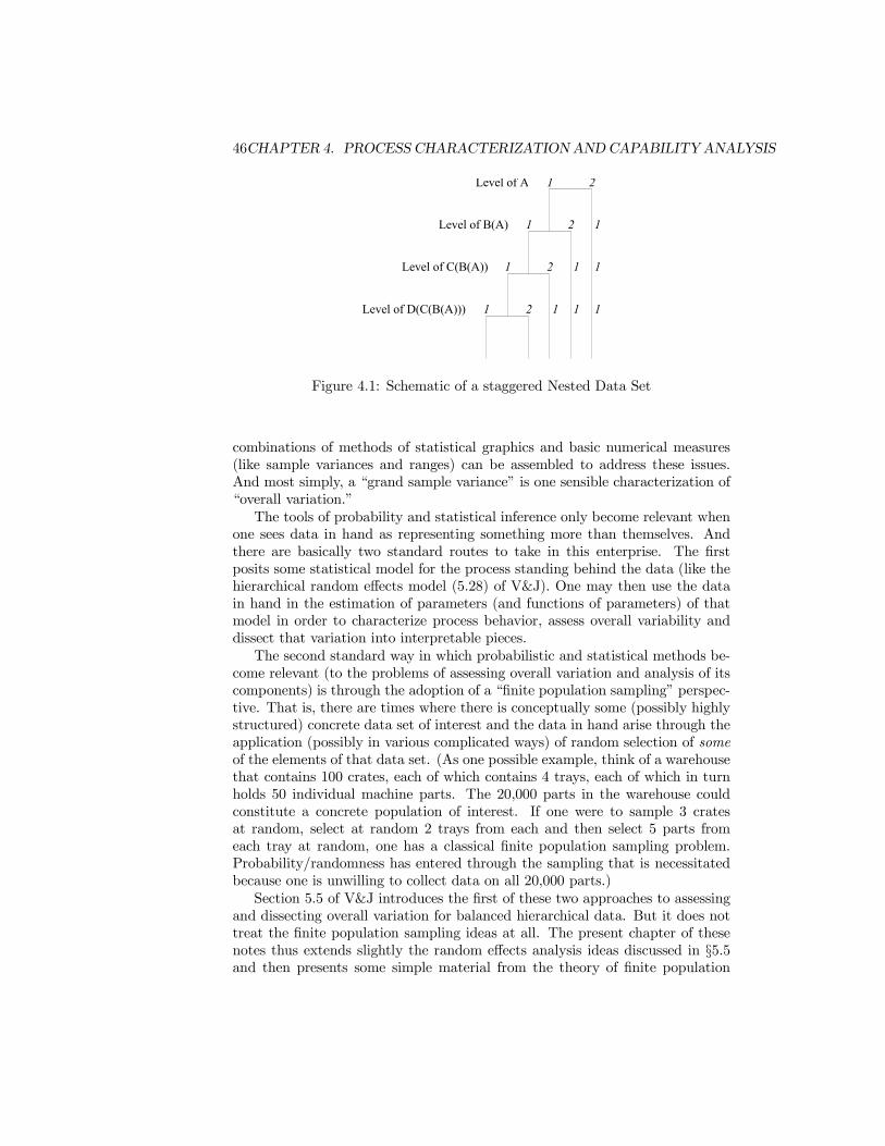
46CHAPTER 4. PROCESS CHARACTERIZATION AND CAPABILITY ANALYSIS
1
1 2
1
1 2 1 1 1
Level of A
Level of B(A)
Level of C(B(A))
Level of D(C(B(A)))
2
1
1 2 1
Figure 4.1: Schematic of a staggered Nested Data Set
combinations of methods of statistical graphics and basic numerical measures(like sample variances and ranges) can be assembled to address these issues.And most simply, a “grand sample variance” is one sensible characterization of“overall variation.”
The tools of probability and statistical inference only become relevant whenone sees data in hand as representing something more than themselves. Andthere are basically two standard routes to take in this enterprise. The …rstposits some statistical model for the process standing behind the data (like thehierarchical random e¤ects model (5.28) of V&J). One may then use the datain hand in the estimation of parameters (and functions of parameters) of thatmodel in order to characterize process behavior, assess overall variability anddissect that variation into interpretable pieces.
The second standard way in which probabilistic and statistical methods be-come relevant (to the problems of assessing overall variation and analysis of itscomponents) is through the adoption of a “…nite population sampling” perspec-tive. That is, there are times where there is conceptually some (possibly highlystructured) concrete data set of interest and the data in hand arise through theapplication (possibly in various complicated ways) of random selection of someof the elements of that data set. (As one possible example, think of a warehousethat contains 100 crates, each of which contains 4 trays, each of which in turnholds 50 individual machine parts. The 20,000 parts in the warehouse couldconstitute a concrete population of interest. If one were to sample 3 cratesat random, select at random 2 trays from each and then select 5 parts fromeach tray at random, one has a classical …nite population sampling problem.Probability/randomness has entered through the sampling that is necessitatedbecause one is unwilling to collect data on all 20,000 parts.)
Section 5.5 of V&J introduces the …rst of these two approaches to assessingand dissecting overall variation for balanced hierarchical data. But it does nottreat the …nite population sampling ideas at all. The present chapter of thesenotes thus extends slightly the random e¤ects analysis ideas discussed in §5.5and then presents some simple material from the theory of …nite population

4.2. MORE ON ANALYSIS UNDER THE HIERARCHICAL RANDOM EFFECTS MODEL47
sampling.
4.2 More on Analysis Under the HierarchicalRandom E¤ects Model
Consider the hierarchical random e¤ects model with 2 levels of nesting discussedin §5.5.2 of V&J. We will continue the notations yijk; ¹yij ; ¹yi: and ¹y:: used inthat section and also adopt some additional notation. For one thing, it will beuseful to de…ne some ranges. Let
Rij = maxk
yijk¡mink
yijk = the range of the jth sample within the ith level of A ;
¢i = maxj
¹yij¡minj
¹yij = the range of the J sample means within the ith level of A ;
and
¡ = maxi
¹yi: ¡ mini
¹yi: = the range of the means for the I levels of A :
It will also be useful to consider the ANOVA sums of squares and meansquares alluded to brie‡y in §5.5.3. So let
SSTot =X
i;j;k
(yijk ¡ ¹y::)2
= (IJK ¡ 1) £ the grand sample variance of all IJK observations ;
SSC(B(A)) =X
i;j;k
(yijk ¡ ¹yij)2
= (K ¡ 1) £ the sum of all IJ “level C” sample variances ;
SSB(A) = KX
i;j
(¹yij ¡ ¹yi:)2
= K(J ¡ 1) £ the sum of all I sample variances of J means ¹yij
and
SSA = KJX
i
(¹yi: ¡ ¹y::)2
= KJ(I ¡ 1) £ the sample variance of the I means ¹yi: :
Note that in the notation of §5.5.2, SSA = KJ(I ¡ 1)s2A, SSB(A) = K(J ¡
1)PI
i=1 s2Bi and SSC(B(A)) = (K ¡ 1)
Pi;j s2
ij = IJ(K ¡ 1)b¾2. And it is analgebraic fact that SSTot = SSA + SSB(A) + SSC(B(A)).
Mean squares are derived from these sums of squares by dividing by appro-priate degrees of freedom. That is, de…ne
MSA :=SSAI ¡ 1
;

48CHAPTER 4. PROCESS CHARACTERIZATION AND CAPABILITY ANALYSIS
MSB(A) :=SSB(A)I(J ¡ 1)
;
andMSC(B(A)) :=
SSC(B(A))IJ(K ¡ 1)
:
Now these ranges, sums of squares and mean squares are interesting measuresof variation in their own right, but are especially helpful when used to produceestimates of variance components and functions of variance components. Forexample, it is straightforward to verify that under the hierarchical random e¤ectsmodel (5.28) of V&J
ERij = d2(K)¾ ;
E¢i = d2(J)q
¾2¯ + ¾2=K
andE¡ = d2(I)
q¾2
® + ¾2¯=J + ¾2=JK :
So, reasoning as in §2.2.2 of V&J (there in the context of two-way random e¤ectsmodels and gage R&R) reasonable range-based point estimates of the variancecomponents are
b¾2 =µ ¹R
d2(K)
¶2
;
b¾2¯ = max
Ã0;
µ ¹¢d2(J)
¶2
¡ b¾2
K
!
and
b¾2® = max
Ã0;
µ¡
d2(I)
¶2
¡ 1J
µ ¹¢d2(J)
¶2!
:
Now by applying linear model theory or reasoning from V&J displays (5.30)and (5.32) and the fact that Es2
ij = ¾2, one can …nd expected values for themean squares above. These are
EMSA = KJ¾2® + K¾2
¯ + ¾2 ;
EMSB(A) = K¾2¯ + ¾2
andEMSC (B(A)) = ¾2 :
And in a fashion completely parallel to the exposition in §1.4 of these notes,standard linear model theory implies that the quantities
IJ(K ¡ 1)MSC(B(A))EMSC(B(A))
;I(J ¡ 1)MSB(A)
EMSB(A)and
(I ¡ 1)MSAEMSA
are independent Â2 random variables with respective degrees of freedom
IJ(K ¡ 1); I(J ¡ 1) and (I ¡ 1) :

4.2. MORE ON ANALYSIS UNDER THE HIERARCHICAL RANDOM EFFECTS MODEL49
Table 4.1: Balanced Data Hierarchical Random E¤ects Analysis ANOVA Table(2 Levels of Nesting)
ANOVA TableSource SS df MS EMSA SSA I ¡ 1 MSA KJ¾2
® + K¾2¯ + ¾2
B(A) SSB(A) I(J ¡ 1) MSB(A) K¾2¯ + ¾2
C(B(A)) SSC(B(A)) IJ(K ¡ 1) MSC(B(A)) ¾2
Total SSTot IJK ¡ 1
These facts about sums of squares and mean squares for the hierarchicalrandom e¤ects model are conveniently summarized in the usual (hierarchicalrandom e¤ects model) ANOVA table (for two levels of nesting), Table 4.1. Fur-ther, the fact that the expected mean squares are simple linear combinationsof the variance components ¾2
®, ¾2¯ and ¾2 motivates the use of linear combina-
tions of mean squares in the estimation of the variance components (as in §5.5.3of V&J). In fact (as indicated in §5.5.3 of V&J) the standard ANOVA-basedestimators
b¾2 =SSC(B(A))IJ(K ¡ 1)
;
b¾2¯ =
1K
maxµ
0;SSB(A)I(J ¡ 1)
¡ b¾2¶
andb¾2
® =1
JKmax
µ0;
SSA(I ¡ 1)
¡ SSB(A)I(J ¡ 1)
¶
are exactly the estimators (described without using ANOVA notation) in dis-plays (5.29), (5.31) and (5.33) of V&J. The virtue of describing them in thepresent terms is to suggest/emphasize that all that was said in §1.4 and §1.5(in the gage R&R context) about making standard errors for functions of meansquares and ANOVA-based con…dence intervals for functions of variance com-ponents is equally true in the present context.
For example, the formula (1.3) of these notes can be applied to derive stan-dard errors for b¾2
¯ and b¾2® immediately above. Or since
¾2¯ =
1K
EMSB(A) ¡ 1K
EMSC(B(A))
and¾2
® =1
JKEMSA ¡ 1
JKEMSB(A)
are both of form (1.4), the material of §1.5 can be used to set con…dence limitsfor these quantities.
As a …nal note in this discussion of the what is possible under the hierarchicalrandom e¤ects model, it is worth noting that while the present discussion hasbeen con…ned to a “balanced data” framework, Problem 4.8 shows that at least

50CHAPTER 4. PROCESS CHARACTERIZATION AND CAPABILITY ANALYSIS
point estimation of variance components can be done in a fairly elementaryfashion even in unbalanced data contexts.
4.3 Finite Population Sampling and BalancedHierarchical Structures
This brief subsection is meant to illustrate the kinds of things that can be donewith …nite population sampling theory in terms of estimating overall variabilityin a (balanced) hierarchical concrete population of items and dissecting thatvariability.
Consider …rst a …nite population consisting of NM items arranged into Nlevels of A, with M levels of B within each level of A. (For example, there mightbe N boxes, each containing M widgets. Or there might be N days, on each ofwhich M items are manufactured.) Let
yij = a measurement on the item at level i of A and level j of B within theith level of A (e.g. the diameter of the jth widget in the ith box) :
Suppose that the quantity of interest is the (grand) variance of all NM mea-surements,
S2 =1
NM ¡ 1
NX
i=1
MX
j=1
(yij ¡ ¹y:)2 :
(This is clearly one quanti…cation of overall variation.)The usual one-way ANOVA identity applied to the NM numbers making up
the population of interest shows that the population variance can be expressedas
S2 =1
NM ¡ 1¡M(N ¡ 1)S2
A + N(M ¡ 1)S2B¢
where
S2A =
1N ¡ 1
NX
i=1
(¹yi ¡ ¹y:)2 = the variance of the N “A level means”
and
S2B =
1N
NX
i=1
0@ 1
M ¡ 1
MX
j=1
(yij ¡ ¹yi)2
1A = the average of the N “within A level variances.”
Suppose that one selects a simple random sample of n levels of A, and for eachlevel of A a simple random sample of m levels of B within A. (For example, onemight sample n boxes and m widgets from each box.) A naive way to estimateS2 is to simply use the sample variance
s2 =1
nm ¡ 1
X(yij ¡ ¹y¤
: )2

4.3. FINITE POPULATION SAMPLING AND BALANCED HIERARCHICAL STRUCTURES51
where the sum is over the nm items selected and ¹y¤: is the mean of those mea-
surements. Unfortunately, this is not such a good estimator. Material fromChapter 10 of Cochran’s Sampling Techniques can be used to show that
Es2 =m(n ¡ 1)nm ¡ 1
S2A +
µn(m ¡ 1)nm ¡ 1
+m(n ¡ 1)nm ¡ 1
µ1m
¡ 1M
¶¶S2
B ;
which is not in general equal to S2.However, it is possible to …nd a linear combination of the sample versions of
S2A and S2
B that has expected value equal to the population variance. That is,let
s2A =
1n ¡ 1
X(¹y¤
i ¡ ¹y¤: )2
= the sample variance of the n sample means (from the sampled levels of A)
and
s2B =
1n
Xµ1
m ¡ 1
X(yij ¡ ¹y¤
i )2¶
= the average of the n sample variances (from the sampled levels of A) :
Then, it turns out that
Es2A = S2
A +µ
1m
¡ 1M
¶S2
B
andEs2
B = S2B :
From this it follows that an unbiased estimator of S2 is the quantity
M(N ¡ 1)NM ¡ 1
s2A +
µN(M ¡ 1)NM ¡ 1
¡ M(N ¡ 1)NM ¡ 1
µ1m
¡ 1M
¶¶s2B :
This kind of analysis can, of course, be carried beyond the case of a singlelevel of nesting. For example, consider the situation with two levels of nest-ing (where both the …nite population and the observed values have balancedhierarchical structure). Then in the ANOVA notation of §4.2 above, take
s2A =
SSA(I ¡ 1)JK
;
s2B =
SSB(A)I(J ¡ 1)K
ands2C =
SSC(B(A))IJ(K ¡ 1)
:

52CHAPTER 4. PROCESS CHARACTERIZATION AND CAPABILITY ANALYSIS
Let S2A; S2
B and S2C be the population analogs of s2
A; s2B and s2
C, and fB andfC be the sampling fractions at the second and third stages of item selection.Then it turns out that
Es2A = S2
A +(1 ¡ fB)
JS2
B +(1 ¡ fC)
JKS2
C ;
Es2B = S2
B +(1 ¡ fC)
KS2
C
andEs2
C = S2C :
So (since the grand population variance, S2, is expressible as a linear combina-tion of S2
A; S2B and S2
C, each of which can be estimated by a linear combinationof s2
A; s2B and s2
C) an unbiased estimator of the population variance can be builtas an appropriate linear combination of s2
A; s2B and s2
C.

Chapter 5
Sampling Inspection
Chapter 8 of V&J treats the subject of sampling inspection, introducing thebasic methods of acceptance sampling and continuous inspection. This chapterextends that discussion somewhat. We consider how (in the fraction noncon-forming context) one can move from single sampling plans to quite generalacceptance sampling plans, we provide a brief discussion of the e¤ects of inspec-tion/measurement error on the real (as opposed to nominal) statistical proper-ties of acceptance sampling plans, and then the chapter closes with an elabo-ration of §8.5 of V&J, providing some more details on the matter of economicarguments in the choice of sampling inspection schemes.
5.1 More on Fraction Nonconforming AcceptanceSampling
Section 8.1 of V&J (and for that matter §8.2 as well) con…nes itself to thediscussion of single sampling plans. For those plans, a sample size is …xed inadvance at some value n, and lot disposal is decided on the basis of inspection ofexactly n items. There are, however, often good reasons to consider acceptancesampling plans whose ultimate sample size depends upon “how the inspecteditems look” as they are examined. (One might, for example, want to considera “double sampling” plan that inspects an initial small sample, terminatingsampling if items look especially good or especially bad so that appropriatelot disposal seems clear, but takes an additional larger sample if the initialone looks “inconclusive” regarding the likely quality of the lot.) This sectionconsiders fraction nonconforming acceptance sampling from the most generalperspective possible and develops the OC, ASN, AOQ and ATI for a generalfraction nonconforming plan.
Consider the possibility of inspecting one item at a time from a lot of N , andafter inspecting each successive item deciding to 1) stop sampling and accept
53

54 CHAPTER 5. SAMPLING INSPECTION
1 4
2
4
6
Xn
Accept
Reject
1
3
5
n
5 632
Figure 5.1: Diagram for the n = 6, c = 2 Single Sampling Plan
the lot, 2) stop sampling and reject the lot or 3) inspect another item. With
Xn = the number of nonconforming items found among the …rst n inspected
a helpful way of thinking about various di¤erent plans in this context is interms of possible paths through a grid of ordered pairs of integers (n;Xn) with0 · Xn · n. Di¤erent acceptance sampling plans then amount to di¤erentchoices of “Accept Boundary” and “Reject Boundary.” Figure 5.1 is a diagramrepresenting a single sampling plan with n = 6 and c = 2, Figure 5.2 is a diagramrepresenting a “doubly curtailed” version of this plan (one that recognizes thatthere is no need to continue inspection after lot disposal has been determined)and Figure 5.3 illustrates a double sampling plan in these terms.
Now on a diagram like those in the …gures, one may very quickly count thenumber of permissible paths from (0; 0) to a point in the grid by (working leftto right) marking each point (n;Xn) in the grid (that it is possible to reach)with the sum of the numbers of paths reaching (n ¡ 1;Xn ¡ 1) and (n ¡ 1;Xn)provided neither of those points is a “stop-sampling point.” (No feasible pathsleave a stop-sampling point. So path counts to them do not contribute to pathcounts for any points to their right.) Figure 5.4 is a version of Figure 5.2 withpermissible movements through the (n;Xn) grid marked by arrows, and pathcounts indicated.
The reason that one cares about the path counts is that for any stop-sampling

5.1. MORE ON FRACTION NONCONFORMING ACCEPTANCE SAMPLING55
Xn
Accept
Reject
1 4
2
1
3
n
5 632
Figure 5.2: Diagram for Doubly Curtailed n = 6, c = 2 Single Sampling Plan
Accept
Reject
Xn
1 4
2
4
1
3
5
n
5 632
Figure 5.3: Diagram for a Small Double Sampling Plan

56 CHAPTER 5. SAMPLING INSPECTION
Xn
Accept
Reject
1 4
2
1
3
n
5 632
1 1
1 2 3 4 4
1 3 6 10 10
10631
1 1
Figure 5.4: Diagram for the Doubly Curtailed Single Sampling Plan with PathCounts Indicated
point (n;Xn), from perspective A
P [reaching (n;Xn)] = (path count from (0,0) to (n;Xn))
¡ N¡nNp¡Xn
¢¡ NNp
¢ ;
while from perspective B
P [reaching (n;Xn)] = (path count from (0,0) to (n;Xn)) pXn(1 ¡ p)n¡Xn :
And these probabilities of reaching the various stop sampling points are thefundamental building blocks of the standard statistical characterizations of anacceptance sampling plan.
For example, with A and R respectively the acceptance and rejection bound-aries, the OC for an arbitrary fraction nonconforming plan is
Pa =X
(n;Xn)2A
P [reaching (n;Xn)] : (5.1)
And the mean number of items sampled (the Average Sample Number) is
ASN =X
(n;Xn)2A[R
nP [reaching (n;Xn)] : (5.2)
Further, under the rectifying inspection scenario, from perspective B
AOQ =X
(n;Xn)2A
(1 ¡ nN
)pP [reaching (n;Xn)] ; (5.3)
from perspective A
AOQ =X
(n;Xn)2A
(p ¡ Xn
N)P [reaching (n;Xn)] (5.4)

5.1. MORE ON FRACTION NONCONFORMING ACCEPTANCE SAMPLING57
andATI = N(1 ¡ Pa) +
X
(n;Xn)2A
nP [reaching (n;Xn)] : (5.5)
These formulas are conceptually very simple and quite universal. The factthat specializing them to any particular choice of acceptance boundary andrejection boundary might have been unpleasant when computations had to bedone “by hand” is largely irrelevant in today’s world of plentiful fast and cheapcomputing. These simple formulas and a personal computer make completelyobsolete the many many pages of specialized formulas that at one time …lledbooks on acceptance sampling.
Two other matters of interest remain to be raised regarding this generalapproach to fraction nonconforming acceptance sampling. The …rst concernsthe di¢cult mathematical question “What are good shapes for the accept andreject boundaries?” We will talk a bit in the …nal section of this chapter aboutcriteria upon which various plans might be compared and allude to how onemight try to …nd a “best” plan (“best” shapes for the acceptance and rejectionboundaries) according to such criteria. But at this point, we wish only tonote that Abraham Wald working in the 1940s on the problem of sequentialtesting, developed some approximate theory that suggests that parallel straightline boundaries (the acceptance boundary below the rejection boundary) havesome attractive properties. He was even able to provide some approximatetwo-point design criteria. That is, in order to produce a plan whose OC curveruns approximately through the points (p1; Pa1) and (p2; Pa2) (for p1 < p2 andPa1 > Pa2) Wald suggested linear stop-sampling boundaries with
slope =ln
³1¡p11¡p2
´
ln³
p2(1¡p1)p1(1¡p2)
´ : (5.6)
An appropriate Xn-intercept for the acceptance boundary is approximately
hA =ln
³Pa1Pa2
´
ln³
p2(1¡p1)p1(1¡p2)
´ ; (5.7)
while an appropriate Xn-intercept for the rejection boundary is approximately
hR =ln
³1¡Pa21¡Pa1
´
ln³
p2(1¡p1)p1(1¡p2)
´ : (5.8)
Wald actually derived formulas (5.6) through (5.8) under “in…nite lot size”assumptions (that also allowed him to produce some approximations for both theOC and ASN of his plans). Where one is thinking of applying Wald’s boundariesin acceptance sampling of a real (…nite N) lot, the question of exactly how totruncate the sampling (close in the right side of the “continue sampling region”)

58 CHAPTER 5. SAMPLING INSPECTION
Xn
1 4
2
1
3
n
5 632
1
1 2
1 2 3 4
443
1 1 1
0
Figure 5.5: Path Counts from (1; 1) to Stop Sampling Points for the Plan ofFigure 5.4
must be answered in some sensible fashion. And once that is done, the basicformulas (5.1) through (5.5) are of course relevant to describing the resultingplan. (See Problem 5.4 for an example of this kind of logic in action.)
Finally, it is an interesting side-light here (that can come into play if onewishes to estimate p based on data from something other than a single samplingplan) that provided the stop-sampling boundary has exactly one more point in itthan the largest possible value of n, the uniformly minimum variance unbiasedestimator of p for both type A and type B contexts is (for (n;Xn) a stop-sampling point)
bp ((n;Xn)) =path count from (1,1) to (n;Xn)path count from (0,0) to (n;Xn)
:
For example, Figure 5.5 shows the path counts from (1,1) needed (in conjunctionwith the path counts indicated in Figure 5.4) to …nd the uniformly minimumvariance unbiased estimator of p when the doubly curtailed single sampling planof Figure 5.4 is used.
Table 5.1 lists the values of bp for the 7 points in the stop-sampling boundaryfor the doubly curtailed single sampling plan with n = 6 and c = 2, along withthe corresponding values of Xn=n (the maximum likelihood estimator of p).
5.2 Imperfect Inspection and Acceptance Sam-pling
The nominal statistical properties of sampling inspection procedures are “per-fect inspection” properties. The OC formulas for the attributes plans in §8.1and §8.4 of V&J and §5.1 above are really premised on the ability to tell withcertainty whether an inspected item is conforming or nonconforming. And theOC formulas for the variables plans in §8.2 of V&J are premised on an assump-tion that the measurement x that determines whether an item is conforming or

5.2. IMPERFECT INSPECTION AND ACCEPTANCE SAMPLING 59
Table 5.1: The UMVUE and MLE of p for the Doubly Curtailed Single SamplingPlan
Stop-sampling point (n;Xn) UMVUE, bp MLE, Xn=n(3; 3) 1=1 3=3(4; 0) 0=1 0=4(4; 3) 2=3 3=4(5; 1) 1=4 1=5(5; 3) 3=6 3=5(6; 2) 4=10 2=6(6; 3) 4=10 3=6
Table 5.2: Perspective B Description of a Single Inspection Allowing fo Inspec-tion Error
Inspection ResultG D
Actual G (1 ¡ wG)(1 ¡ p) wG(1 ¡ p) 1 ¡ pCondition D pwD p(1 ¡ wD) p
1 ¡ p¤ p¤
nonconforming can be obtained for a given item completely without measure-ment error. But the truth is that real-world inspection is not perfect and thenominal statistical properties of these methods at best approximate their actualproperties. The purpose of this section is to investigate (…rst in the attributescontext and then in the variables context) just how far actual OC values forcommon acceptance sampling plans can be from nominal ones.
Consider …rst the percent defective context and suppose that when a con-forming (good) item is inspected, there is a probability wG of misclassifying it asnonconforming. Similarly, suppose that when a nonconforming (defective) itemis inspected, there is a probability wD of misclassifying it as conforming. Thenfrom perspective B, a probabilistic description of any single inspected item isgiven in Table 5.2, where in that table we are using the abbreviation
p¤ = wG(1 ¡ p) + p(1 ¡ wD)
for the probability that an item (of unspeci…ed actual condition) is classi…ed asnonconforming by the inspection process.
It should thus be obvious that from perspective B in the fraction noncon-forming context, an attributes single sampling plan with sample size n andacceptance number c has an actual acceptance probability that depends notonly on p but on wG and wD as well through the formula
Pa(p;wG; wD) =cX
x=0
µnx
¶(p¤)x (1 ¡ p¤)n¡x : (5.9)
On the other hand, the perspective A version of the fraction nonconformingscenario yields the following. For an integer x from 0 to n, let Ux and Vx be

60 CHAPTER 5. SAMPLING INSPECTION
independent random variables,
Ux » Binomial (x; 1 ¡ wD) and Vx » Binomial (n ¡ x;wG) :
And letrx = P [Ux + Vx · c]
be the probability that a sample containing x nonconforming items actuallypasses the lot acceptance criterion. (Note that the nonstandard distribution ofUx+Vx can be generated using the same “adding on diagonals of a table of jointprobabilities” idea used in §1.7.1 to generate the distribution of x.) Then it isevident that from perspective A an attributes single sampling plan with samplesize n and acceptance number c has an actual acceptance probability
Pa(p;wG; wD) =nX
x=0
¡Npx
¢¡N(1¡p)n¡x
¢¡N
n
¢ rx : (5.10)
It is clear that nonzero wG or wD change nominal OC’s given in displays (8.6)and (8.5) of V&J into the possibly more realistic versions given respectively byequations (5.9) and (5.10) here. In some cases, it may be possible to determinewG and wD experimentally and therefore derive both nominal and “real” OCcurves for a fraction nonconforming single sampling plan. Or, if one were apriori willing to guarantee that 0 · wG · a and that 0 · wD · b, it is prettyclear that from perspective B one might then at least guarantee that
Pa(p; a; 0) · Pa(p;wG; wD) · Pa(p; 0; b) (5.11)
and have an “OC band” in which the real OC (that depends upon the unknowninspection e¢cacy) is guaranteed to lie.
Similar analyses can be done for nonconformities per unit contexts as follows.Suppose that during inspection of product, real nonconformities are missedwith probability m and that (independent of the occurrence and inspectionof real nonconformities) “phantom” nonconformities are “observed” accordingto a Poisson process with rate ¸P per unit inspected. Then from perspective Bin a nonconformities per unit context, the number of nonconformities observedon k units is Poisson with mean
k(¸(1 ¡ m) + ¸P) ;
so that an actual acceptance probability corresponding to the nominal one givenin display (8.8) of V&J is
Pa(¸; ¸P;m) =cX
x=0
exp (¡k(¸(1 ¡ m) + ¸P)) (k(¸(1 ¡ m) + ¸P))x
x!: (5.12)
And from perspective A, with a realized per unit defect rate ¸ on N units,let U¸;m » Binomial (k¸;
¡ kN
¢(1 ¡ m)) be independent of V¸P » Poisson (k¸P).

5.2. IMPERFECT INSPECTION AND ACCEPTANCE SAMPLING 61
Then an actual acceptance probability corresponding to the nominal one givenin display (8.7) of V&J is
Pa(¸; ¸P;m) = P [U¸;m + V¸P · c] : (5.13)
And the same kinds of bounding ideas used above for the fraction nonconformingcontext might be used with the OC (5.12) in the mean nonconformities per unitcontext. Pretty clearly, if one could guarantee that ¸P · a and that m · b, onewould have (from display (5.12))
Pa(¸; a; 0) · Pa(¸; ¸P;m) · Pa(¸; 0; b) (5.14)
in the perspective B situation.The violence done to the OC notion by the possibility of imperfect inspec-
tion in an attributes sampling context is serious, but not completely unman-ageable. That is, where one can determine the likelihood of inspection errorsexperimentally, expressions (5.9), (5.10), (5.12) and (5.13) are simple enoughcharacterizations of real OC’s. And where wG and wD (or ¸P and m) are small,bounds like (5.11) (or (5.14)) show that both the nominal (the wG = 0 andwD = 0, or ¸P = 0 and m = 0 case) OC and real OC are trapped in a fairlynarrow band and can not be too di¤erent. Unfortunately, the situation is farless happy in the variables sampling context.
The origin of the di¢culty with admitting there is measurement error whenit comes to variables acceptance sampling is the fundamental fact that standardvariables plans attempt to treat all (¹; ¾) pairs with the same value of p equally.And in short, once one admits to the possibility of measurement error cloudingthe evaluation of the quantity x that must say whether a given item is conform-ing or nonconforming, that goal is unattainable. For any level of measurementerror, there are (¹; ¾) pairs (with very small ¾) for which product variation canso to speak “hide in the measurement noise.” So some fairly bizarre real OCproperties result for standard plans.
To illustrate, consider the case of “unknown ¾” variables acceptance sam-pling with a lower speci…cation, L and adopt the basic measurement model(2.1) of V&J for what is actually observed when an item with characteristic xis measured. Now the development in §8.2 of V&J deals with a normal (¹; ¾)distribution for observations. An important issue is “What observations?” Is itthe x’s or the y’s of the model (2.1)? It must be the x’s, for the simple reasonthat p is de…ned in terms of ¹ and ¾. These parameters describe what the lotis really like, NOT what it looks like when measured with error. That is, the¾ of §8.2 of V&J must be the ¾x of page 19 of V&J. But then the analysis of§8.2 is done essentially supposing that one has at his or her disposal ¹x and sxto use for decision making purposes, while all that is really available are ¹y andsy!!! And that turns out to make a huge di¤erence in the real OC properties ofthe standard method put forth in §8.2.
That is, applying criterion (8.35) of V&J to what can really be observed(namely the noise-corrupted y’s) one accepts a lot i¤
¹y ¡ L ¸ ksy : (5.15)

62 CHAPTER 5. SAMPLING INSPECTION
And under model (2.1) of V&J, a given set of parameters (¹x; ¾x) for the xdistribution has corresponding fraction nonconforming
p(¹x; ¾x) = ©µ
L ¡ ¹x
¾x
¶
and acceptance probability
Pa(¹x; ¾x; ¯; ¾measurement) = P·
¹y ¡ Lsy
¸ k¸
= P
0@
¹y¡¹y
¾y=p
n ¡ L¡¹y
¾y=p
nsy¾y
¸ kp
n
1A
where ¾y is given in display (2.3) of V&J. But then let
¢ = ¡L ¡ ¹y
¾y=p
n= ¡ (L ¡ ¹x)=¾x ¡ ¯=¾xq
1 + ¾2measurement
¾2x
=p
n; (5.16)
and note that¹y ¡ ¹y
¾y=p
n» Normal (0; 1)
independent of sy¾y
, which has the distribution ofp
U=(n ¡ 1) for U a Â2n¡1
random variable. That is, with W a noncentral t random variable with noncen-trality parameter ¢ given in display (5.16), we have
Pa(¹x; ¾x; ¯; ¾measurement) = P [W ¸ kp
n] :
And the crux of the matter is that (even if measurement bias, ¯, is 0) ¢ indisplay (5.16) is not a function of (L ¡ ¹x)=¾x alone unless one assumes that¾measurement is EXACTLY 0.
Even with no measurement bias, if ¾measurement 6= 0 there are (¹x; ¾x) pairswith
L ¡ ¹x
¾x= z
(and therefore p = ©(z)) and ¢ ranging all the way from ¡zp
n to 0. Thusconsidering z · 0 and p · :5 there are corresponding Pa’s ranging from
P [a tn¡1 random variable ¸ kp
n]
toP [a non-central tn¡1(¡z
pn) random variable ¸ k
pn] ;
(the nominal OC), while considering z ¸ 0 and p ¸ :5 there are correspondingPa’s ranging from (the nominal OC)
P [a non-central tn¡1(¡zp
n) random variable ¸ kp
n] ;

5.3. SOME DETAILS CONCERNING THE ECONOMIC ANALYSIS OF SAMPLING INSPECTION63
p.5
1.0
Pa(p)
Figure 5.6: Typical Real OC for a One-Sided Variables Acceptance SamplingPlan in the Presence of Nonzero Measurement Error
toP [a tn¡1 random variable ¸ k
pn] :
That is, one is confronted with the extremely unpleasant and (initially counter-intuitive) picture of real OC indicated in Figure 5.6.
It is important to understand the picture painted in Figure 5.6. The situationis worse than in the attributes data case. There, if one knows the e¢cacy ofthe inspection methodology it is at least possible to pick a single appropriateOC curve. (The OC “bands” indicated by displays (5.11) and (5.14) are createdonly by ignorance of inspection e¢cacy.) The bizarre “OC bands” created inthe variables context (and sketched in Figure 5.6) do not reduce to curves if oneknows the inspection bias and precision, but rather are intrinsic to the fact thatunless ¾measurement is exactly 0, di¤erent (¹; ¾) pairs with the same p must havedi¤erent Pa’s under acceptance criterion (5.15). And the only way that one canreplace the situation pictured in Figure 5.6 with one having a thinner and morepalatable OC band (something approximating a “curve”) is by guaranteeingthat
¾2x
¾2measurement
is of some appreciable size. That is, given a particular measurement precision,one must agree to concern oneself only with cases where product variation cannothide in measurement noise. Such is the only way that one can even come closeto the variables sampling goal of treating (¹; ¾) pairs with the same p equally.
5.3 Some Details Concerning the Economic Analy-sis of Sampling Inspection
Section 8.5 of V&J alludes brie‡y to the possibility of using economic/decision-theoretic arguments in the choice of sampling inspection schemes and cites the1994 Technometrics paper of Vander Wiel and Vardeman. Our …rst objective

64 CHAPTER 5. SAMPLING INSPECTION
in this section is to provide some additional details of the Vander Wiel andVardeman analysis. To that end, consider a stable process fraction noncon-forming situation and continue the wG and wD notation used above (and alsointroduced on page 493 of V&J). Note that Table 5.2 remains an appropriatedescription of the results of a single inspection. We will suppose that inspectioncosts are accrued on a per item basis and adopt the notation of Table 8.16 ofV&J for the costs.
As a vehicle to a very quick demonstration of the famous “all or none”principle, consider facing N potential inspections and employing a “randominspection policy” that inspects each item independently with probability ¼.Then the mean cost su¤ered over N items is simply N times that su¤ered for 1item. And this is
ECost = ¼ (kI + (1 ¡ p)wGkGF + p(1 ¡ wD)kDF + pwDkDP) + (1 ¡ ¼)pkDU
= ¼(kI + wGkGF ¡ pK) + pkDU (5.17)
forK = (1 ¡ wD)(kDU ¡ kDF) + wD(kDU ¡ kDP) + wGkGF
(as in display (8.50) of V&J). Now it is clear from display (5.17) that if K < 0,ECost is minimized over choices of ¼ by the choice ¼ = 0. On the other hand,if K > 0, ECost is minimized over choices of ¼
by the choice ¼ = 0 if p · kI + wGkGF
K
andby the choice ¼ = 1 if p ¸ kI + wGkGF
K:
That is, if one de…nes
pc =½ 1 if K · 0
kI+wGkGFK if K > 0
then an optimal random inspection policy is clearly
¼ = 0 (do no inspection) if p < pc
and¼ = 1 (inspect everything) if p > pc :
This development is simple and completely typical of what one gets from eco-nomic analyses of stable process (perspective B) inspection scenarios. Wherequality is poor, all items should be inspected, and where it is good none shouldbe inspected. Vander Wiel and Vardeman argue that the speci…c criterion de-veloped here (and phrased in terms of pc) holds not only as one looks for anoptimal random inspection policy, but completely generally as one looks amongall possible inspection policies for one that minimizes expected total cost. Butit is essential to remember that the context is a stable process/perspective B

5.3. SOME DETAILS CONCERNING THE ECONOMIC ANALYSIS OF SAMPLING INSPECTION65
context, where costs are accrued on a per item basis, and in order to implementthe optimal policy one must know p! In other contexts, the best (minimumexpected cost) implementable/realizable policy will often turn out to not be ofthe “all or none” variety. The remainder of this section will elaborate on thisassertion.
For the balance of the section we will consider (Barlow’s formulation) ofwhat we’ll call the “Deming Inspection Problem” (as Deming’s considerationof this problem rekindled interest in these matters and engendered considerablecontroversy and confusion in the 1980s and early 1990s). That is, we’ll considera lot of N items, assume a cost structure where
k1 = the cost of inspecting one item (at the proposed inspection site)
and
k2 = the cost of later grief caused by a defective item that is not detected
and suppose that inspection is without error. (This is the Vander Wiel andVardeman cost structure with kI = k1; kDF = 0 and kDU = k2, where bothwG and wD are assumed to be 0.) The objective will be optimal (minimumexpected cost) choice of a “…xed n inspection plan” (in the language of §8.1of V&J, a single sampling with recti…cation plan). That is, we’ll consider theoptimal choice of n and c supposing that with
X = the number nonconforming in a sample of n ;
if X · c the lot will be “accepted” (all nonconforming items in the samplewill be replaced with good ones and no more inspection will be done), whileif X > c the lot will be “rejected” (all items in the lot will be inspected andall nonconforming items replaced with good ones). (The implicit assumptionhere is that replacements for nonconforming items are somehow known to beconforming and are produced “for free.”) And we will continue use of the stableprocess or perspective B model for the generation of the items in the lot.
In this problem, the expected total cost associated with the lot is a functionof n, c and p,
ETC(n; c; p) = k1n + (1 ¡ Pa(n; c; p))k1(N ¡ n) + pPa(n; c; p)k2(N ¡ n)
= k1Nµ
1 + Pa(n; c; p)³1 ¡ n
N
´µpk2
k1¡ 1
¶¶: (5.18)
Optimal choice of n and c requires that one be in the business of comparing thefunctions of p de…ned in display (5.18). How one approaches that comparisondepends upon what one is willing to input into the decision process in terms ofinformation about p.
First, if p is …xed/known and available for use in choosing n and c, the op-timization of criterion (5.18) is completely straightforward. It amounts only tothe comparison of numbers (one for each (n; c) pair), not functions. And the

66 CHAPTER 5. SAMPLING INSPECTION
solution is quite simple. In the case that p > k1=k2,³pk2
k1¡ 1
´> 0 and from
examination of display (5.18) minimum expected total cost will be achieved ifPa(n; c; p) = 0 or if
¡1 ¡ n
N
¢= 0. That is, “all” is optimal. In the case that
p < k1=k2,³pk2
k1¡ 1
´< 0 and from examination of formula (5.18) minimum
expected total cost will be achieved if Pa(n; c; p) = 1 and¡1 ¡ n
N
¢= 1. That
is, “none” is optimal. This is a manifestation of the general Vander Wiel andVardeman result. For known p in this kind of problem, sampling/partial in-spection makes no sense. One is not going to learn anything about p from thesampling. Simple economics (comparison of p to the critical cost ratio k1=k2)determines whether it is best to inspect and rectify, or to “take one’s lumps” inlater costs.
When one may not assume that p is …xed/known (and it is thus unavail-able for use in choosing an optimal (n; c) pair) some other approach has to betaken. One possibility is to describe p with a probability distribution G, averageETC(n; c; p) over p according to that distribution to get EGETC(n; c), and thento compare numbers (one for each (n; c) pair) to identify an optimal inspectionplan. This makes sense
1. from a Bayesian point of view, where the distribution G re‡ects one’s“prior beliefs” about p, or
2. from a non-Bayesian point of view, where the distribution G is a “processdistribution” describing how p is thought to vary lot to lot.
The program SAMPLE (written by Tom Lorenzen and modi…ed slightly bySteve Crowder) available o¤ the Stat 531 Web page will do this averaging andoptimization for the case where G is a Beta distribution.
Consider what insights into this “average out according to G” idea can bewritten down in more or less explicit form. In particular, consider …rst theproblem of choosing a best c for a particular n, say (copt
G (n)). Note that if asample of n results in xnonconforming items, the (conditional) expected costincurred is
nk1 + (N ¡ n)k2EG[p jX = x] with no more inspection
andNk1 if the remainder of the lot is inspected :
(Note that the form of the conditional mean of p given X = x depends uponthe distribution G.) So, one should do no more inspection if
nk1 + (N ¡ n)k2EG[p jX = x] < Nk1 ;
i.e. if
EG[p jX = x] <k1
k2;

5.3. SOME DETAILS CONCERNING THE ECONOMIC ANALYSIS OF SAMPLING INSPECTION67
and the remaining items should be inspected if
EG[p jX = x] >k1
k2:
So, an optimal choice of c is
coptG (n) = max
½x j EG[p j X = x] · k1
k2
¾: (5.19)
(And it is perhaps comforting to know that the monotone likelihood ratio prop-erty of the binomial distribution guarantees that EG[p jX = x] is monotone inx.)
What is this saying? The assumptions 1) that p » G and 2) that conditionalon p the variable X » Binomial (n; p) together give a joint distribution for p andX. This in turn can be used to produce for each x a conditional distributionof pjX = x and therefore a conditional mean value of p given that X = x.The prescription (5.19) says that one should …nd the largest x for which thatconditional mean value of p is still less than the critical cost ratio and use thatvalue for copt
G (n). To complete the optimization of EGETC(n; c; p), one thenwould then need to compute and compare (for various n) the quantities
EGETC(n; coptG (n); p) : (5.20)
The fact is that depending upon the nature of G, the minimizer of quantity(5.20) can turn out to be anything from 0 to N . For example, if G puts all itsprobability on one side or the other of k1=k2, then the conditional distributionsof p given X = x must concentrate all their probability (and therefore havetheir means) on that same side of the critical cost ratio. So it follows that if Gputs all its probability to the left of k1=k2, “none” is optimal (even though onedoesn’t know p exactly), while if G puts all its probability to the right of k1=k2,“all” is optimal in terms of optimizing EGETC(n; c; p).
On the other hand, consider an unrealistic but instructive situation wherek1 = 1; k2 = 1000 and G places probability 1
2 on the possibility that p = 0 andprobability 1
2 on the possibility that p = 1. Under this model the lot is eitherperfectly good or perfectly bad, and a priori one thinks these possibilities areequally likely. Here the distribution G places probability on both sides of thebreakeven quantity k1=k2 = :001. Even without actually carrying through thewhole mathematical analysis, it should be clear that in this scenario the optimaln is 1! Once one has inspected a single item, he or she knows for sure whetherp is 0 or is 1 (and the lot can be recti…ed in the latter case).
The most common mathematically nontrivial version of this whole analysisof the Deming Inspection Problem is the case where G is a Beta distribution.If G is the Beta(®; ¯) distribution,
EG[p jX = x] =® + x
® + ¯ + n

68 CHAPTER 5. SAMPLING INSPECTION
so that coptG (n) is the largest value of x such that
® + x® + ¯ + n
· k1
k2:
That is, in this situation, for byc the greatest integer in y,
coptG (n) = bk1
k2(® + ¯ + n) ¡ ®c = bk1
k2n ¡ ® +
k1
k2(® + ¯)c ;
which for large n is essentially k1k2
n. The optimal value of n can then be foundby optimizing (over choice of n) the quantity
EG¡ETC(n; copt
G (n); p)¢
=Z 1
0ETC(n; copt
G (n); p)1
B(®; ¯)p®¡1(1 ¡ p)¯¡1dp :
The reader can check that this exercise boils down to the minimization over nof
³1 ¡ n
N
´ coptG (n)X
x=0
µnx
¶Z 1
0px(1 ¡ p)n¡x
µpk2
k1¡ 1
¶p®¡1(1 ¡ p)¯¡1dp :
(The SAMPLE program of Lorenzen alluded to earlier actually uses a di¤erentapproach than the one discussed here to …nd optimal plans. That approach iscomputationally more e¢cient, but not as illuminating in terms of laying barethe basic structure of the problem as the route taken in this exposition.)
As two …nal pieces of perspective on this topic of economic analysis of sam-pling inspection we o¤er the following. In the …rst place, while the DemingInspection Problem is not a terribly general formulation of the topic, the resultshere are typical of how things turn out. Second, it needs to be remembered thatwhat has been described here is the …nding of a cost-optimal …xed n inspectionplan. The problem of …nding a plan optimal among all possible plans (of thetype discussed in §5.1) is a more challenging one. For G placing probabilityon both sides of the critical cost ratio, not only need it not be that case that“all” or “none” is optimal, but in general an optimal plan need not be of the…xed n variety. While in principle the methodology for …nding an overall bestinspection plan is well-established (involving as it does so called “dynamic pro-gramming” or “backwards induction”) the details are unpleasant enough thatit will not make sense to pursue this matter further.

Chapter 6
Problems
1 Measurement and Statistics
1.1. Suppose that a sample variance s2 is based on a sample of size n from anormal distribution. One might consider estimating ¾ using s or s=c4(n),or even some other multiple of s.
(a) Since c4(n) < 1, the second of these estimators has a larger variancethan the …rst. But the second is unbiased (has expected value ¾)while the …rst is not. Which has the smaller mean squared error,E(b¾ ¡ ¾)2? Note that (as is standard in statistical theory), E(b¾ ¡¾)2 =Var b¾+(Eb¾¡¾)2. (Mean squared error is variance plus squaredbias.)
(b) What is an optimal (in terms of minimum mean squared error) mul-tiple of s to use in estimating ¾?
1.2. How do R=d2(n) and s=c4(n) compare (in terms of mean squared error)as estimators of ¾? (The assumption here is that they are both based ona sample from a normal distribution. See Problem 1.1 for a de…nition ofmean squared error.)
1.3. Suppose that sample variances s2i , i = 1; 2; : : : ; r are based on independent
samples of size m from normal distributions with a common standarddeviation, ¾. A common SQC-inspired estimator of ¾ is ¹s=c4(m). Anotherpossibility is
spooled =
sµs21 + ¢ ¢ ¢ + s2
r
r
¶
69

70 CHAPTER 6. PROBLEMS
or¾ = spooled=c4((m ¡ 1)r + 1) :
Standard distribution theory says that r(m¡ 1)s2pooled=¾2 has a Â2 distri-
bution with r(m ¡ 1) degrees of freedom.
(a) Compare ¹s=c4(m), spooled and ¾ in terms of mean squared error.
(b) What is an optimal multiple of spooled (in terms of mean squarederror) to use in estimating ¾?
(Note: See Vardeman (1999 IIE Transactions) for a complete treatmentof the issues raised in Problems 1.1 through 1.3.)
1.4. Set up a double integral that gives the probability that the sample rangeof n standard normal random variables is between .5 and 2.0. How isthis probability related to the probability that the sample range of n iidnormal (¹; ¾2) random variables is between .5¾ and 2.0¾?
1.5. It is often helpful to state “standard errors” (estimated standard devi-ations) corresponding to point estimates of quantities of interest. In acontext where a standard deviation, ¾, is to be estimated by ¹R=d2(n)based on r samples of size n, what is a reasonable standard error to an-nounce? (Be sure that your answer is computable from sample data, i.e.doesn’t involve any unknown process parameters.)
1.6. Consider the paper weight data in Problem (2.12) of V&J. Assume thatthe 2-way random e¤ects model is appropriate and do the following.
(a) Compute the ¹yij ; sij and Rij for all I£J = 2£5 = 10 Piece£Operatorcombinations. Then compute both row ranges of means ¢i and rowsample variances of means s2
i .
(b) Find both range-based and sample variance-based point estimates ofthe repeatability standard deviation, ¾.
(c) Find both range-based and sample variance-based point estimates ofthe reproducibility standard deviation ¾reproducibility =
q¾2
¯ + ¾2®¯ .
(d) Get a statistical package to give you the 2-way ANOVA table for thesedata. Verify that s2
pooled = MSE and that your sample variance-based estimate of ¾reproducibility from part (c) is
smax
µ0;
1mI
MSB +I ¡ 1mI
MSAB ¡ 1m
MSE¶
:

1. MEASUREMENT AND STATISTICS 71
(e) Find a 90% two-sided con…dence interval for the parameter ¾.
(f) Use the material in §1.5 and give an approximate 90% two-sidedcon…dence interval for ¾reproducibility.
(g) Find a linear combination of the mean squares from (d) whose ex-pected value is ¾2
overall = ¾2reproducibility + ¾2. All the coe¢cients in
your linear combination will be positive. In this case, the you may usethe next to last paragraph of §1.5 to come up with an approximate90% two-sided con…dence interval for ¾overall. Do so.
(h) The problem from which the paper weight data are drawn indicatesthat speci…cations of approximately §4g/m2 are common for paperof the type used in this gage study. These translate to speci…cationsof about §:16g for pieces of paper of the size used here. Use thesespeci…cations and your answer to part (g) to make an approximate90% con…dence interval for the gage capability ratio
GCR =6¾overall
(U ¡ L):
Used in the way it was in this study, does the scale seem adequateto check conformance to such speci…cations?
(i) Give (any sensible) point estimates of the fractions of the overall mea-surement variance attributable to repeatability and to reproducibil-ity.
1.7. In a particular (real) thorium detection problem, measurement variationfor a particular (spectral absorption) instrument was thought to be about¾measurement = :002 instrument units. (Division of a measurement ex-pressed in instrument units by 58.2 gave values in g/l.) Suppose that inan environmental study, a …eld sample is to be measured once (producingynew) on this instrument and the result is to be compared to a (contem-poraneous) measurement of a lab “blank” (producing yold). If the …eldreading exceeds the blank reading by too much, there will be a declarationthat there is a detectable excess amount of thorium present.
(a) Assuming that measurements are normal, …nd a critical value Lc sothat the lab will run no more than a 5% chance of a “false positive”result.
(b) Based on your answer to (a), what is a “lower limit of detection,”Ld, for a 90% probability (°) of correctly detecting excess thorium?What, by the way, is this limit in terms of g/l?
72 CHAPTER 6. PROBLEMS
1.8. Below are 4 hypothetical samples of size n = 3. A little calculation showsthat ignoring the fact that there are 4 samples and simply computing “s”based on 12 observations will produce a “standard deviation” much largerthan spooled. Why is this?
3,6,5 4,3,1 8,9,6 2,1,4
1.9. In applying ANOVA methods to gage R&R studies, one often uses linearcombinations of independent mean squares as estimators of their expectedvalues. Section 1.5 of these notes shows it is possible to also produce stan-dard errors (estimated standard deviations) for these linear combinations.
Suppose that MS1;MS2; : : : ;MSk are independent random variables,ºiMSi
EMSi»
Â2ºi
. Consider the random variable
U = c1MS1 + c2MS2 + ¢ ¢ ¢ + ckMSk :
(a) Find the standard deviation of U .
(b) Your expression from (a) should involve the means EMSi, that inapplications will be unknown. Propose a sensible (data-based) es-timator of the standard deviation of U that does not involve thesequantities.
(c) Apply your result from (b) to give a sensible standard error for theANOVA-based estimators of ¾2, ¾2
reproducibility and ¾2overall.
1.10. Section 1.7 of the notes presents “rounded data” likelihood methods fornormal data with the 2 parameters ¹ and ¾. The same kind of thing can bedone for other families of distributions (which can have other numbers ofparameters). For example, the exponential distributions with means µ¡1
can be used. (Here there is the single parameter µ.) These exponentialdistributions have cdf’s
Fµ(x) =½
1 ¡ exp(¡µx) for x ¸ 00 for x < 0 :
Below is a frequency table for twenty exponential observations that havebeen rounded to the nearest integer.rounded value 0 1 2 3 4
frequency 7 8 2 2 1
(a) Write out an expression for the appropriate “rounded data log like-lihood function” for this problem,
L(µ) = lnL(datajµ) :

1. MEASUREMENT AND STATISTICS 73
(You should be slightly careful here. Exponential random variablesonly take values in the interval (0;1).)
(b) Make a plot of L(µ). Use it and identify the maximum likelihoodestimate of µ based on the rounded data.
(c) Use the plot from (b) and make an approximate 90% con…dence in-terval for µ. (The appropriate Â2 value has 1 associated degree offreedom.)
1.11. Below are values of a critical dimension (in .0001 inch above nominal)measured on hourly samples of size n = 5 precision metal parts takenfrom the output of a CNC (computer numerically controlled) lathe.
sample 1 2 3 4 5 6 7 8measurements 4,3,3,2,3 2,2,3,3,2 4,1,0,¡1,0 2,0,2,1,4 2,2,1,3,4 2, ¡2,2,1,2 0,0,0,2,0 1,¡1,2,0,2
(a) Compute for each of these samples the “raw” sample standard devi-ation (ignoring rounding) and the “Sheppard’s correction” standarddeviation that is appropriate for integer rounded data. How do thesecompare for the eight samples above?
(b) For each of the samples that have a range of at least 2, use the CON-EST program to …nd “rounded normal data” maximum likelihoodestimates of the normal parameters ¹ and ¾. The program as writ-ten accepts observations ¸ 1, so you will need to add an integer toeach element of some of the samples above before doing calculationwith the program. (I don’t remember, but you may not be able to in-put a standard deviation of exactly 0 either.) How do the maximumlikelihood estimates of ¹ compare to ¹x values? How do the max-imum likelihood estimates of ¾ compare to both the raw standarddeviations and to the results of applying “Sheppard’s correction”?
(c) Consider sample #2. Make 95% and 90% con…dence intervals forboth ¹ and ¾ using the work of Johnson Lee.
(d) Consider sample #1. Use the CONEST program to get a few ap-proximate values for L¤(¹) and some approximate values for L¤¤(¾).(For example, look at a contour plot of L over a narrow range ofmeans near ¹ to get an approximate value for L¤(¹).) Sketch L¤(¹)and L¤¤(¾) and use your sketches and Lee’s tables to produce 95%con…dence intervals for ¹ and ¾.
(e) What 95% con…dence intervals for ¹ and ¾ would result from a 9thsample, f2; 2; 2; 2; 2g?

74 CHAPTER 6. PROBLEMS
1.12. A single operator measures a single widget diameter 15 times and obtainsa range of R = 3 £ 10¡4 inches. Then this person measures the diametersof 12 di¤erent widgets once each and obtains a range of R = 8 £ 10¡4
inches. Give an estimated standard deviation of widget diameters (notincluding measurement error).
1.13. Cylinders of (outside) diameter O must …t in ring bearings of (inside)diameter I, producing clearance C = I ¡ O. We would like to havesome idea of the variability in actual clearances that will be obtained by“random assembly” of cylinders produced on one production line with ringbearings produced on another. The gages used to measure I and O are(naturally enough) di¤erent.
In a study using a single gage to measure outside diameters of cylinders,nO = 10 di¤erent cylinders were measured once each, producing a samplestandard deviation sO = :001 inch. In a subsequent study, this samegage was used to measure the outside diameter of an additional cylindermO = 5 times, producing a sample standard deviation sOgage = :0005inch.
In a study using a single gage to measure inside diameters of ring bearings,nI = 20 di¤erent inside diameters were measured once each, producinga sample standard deviation sI = :003 inch. In a subsequent study, thissame gage was used to measure the inside diameter of another ring bearingmI = 10 times, producing a sample standard deviation sIgage = :001 inch.
(a) Give a sensible (point) estimate of the standard deviation of C pro-duced under random assembly.
(b) Find a sensible standard error for your estimate in (a).
2 Process Monitoring
Methods2.1. Consider the following hypothetical situation. A “variables” process mon-
itoring scheme is to be set up for a production line, and two di¤erentmeasuring devices are available for data gathering purposes. Device Aproduces precise and expensive measurements and device B produces lessprecise and less expensive measurements. Let ¾measurement for the twodevices be respectively ¾A and ¾B, and suppose that the target for a par-ticular critical diameter for widgets produced on the line is 200.0.

2. PROCESS MONITORING 75
(a) A single widget produced on the line is measured n = 10 times witheach device and RA = 2:0 and RB = 5:0. Give estimates of ¾A and¾B.
(b) Explain why it would not be appropriate to use one of your estimatesfrom (a) as a “¾” for setting up an ¹x and R chart pair for monitoringthe process based on measurements from one of the devices.
Using device A, 10 consecutive widgets produced on the line (underpresumably stable conditions) have (single) measurements with R =8:0.
(c) Set up reasonable control limits for both ¹x and R for the future mon-itoring of the process based on samples of size n = 10 and measure-ments from device A.
(d) Combining the information above about the A measurements on 10consecutive widgets with your answer to (a), under a model that says
observed diameter = real diameter + measurement error
where “real diameter” and “measurement error” are independent,give an estimate of the standard deviation of the real diameters. (Seethe discussion around page 19 of V&J.)
(e) Based on your answers to parts (a) and (d), set up reasonable controllimits for both ¹x and R for the future monitoring of the process basedon samples of size n = 5 and measurements from the cheaper device,device B.
2.2. The following are some data taken from a larger set in Statistical QualityControl by Grant and Leavenworth, giving the drained weights (in ounces)of contents of size No. 21
2 cans of standard grade tomatoes in puree. 20samples of three cans taken from a canning process at regular intervalsare represented.

76 CHAPTER 6. PROBLEMS
Sample x1 x2 x31 22.0 22.5 22.52 20.5 22.5 22.53 20.0 20.5 23.04 21.0 22.0 22.05 22.5 19.5 22.56 23.0 23.5 21.07 19.0 20.0 22.08 21.5 20.5 19.09 21.0 22.5 20.0
10 21.5 23.0 22.0
Sample x1 x2 x311 20.0 19.5 21.012 19.0 21.0 21.013 19.5 20.5 21.014 20.0 21.5 24.015 22.5 19.5 21.016 21.5 20.5 22.017 19.0 21.5 23.018 21.0 20.5 19.519 20.0 23.5 24.020 22.0 20.5 21.0
(a) Suppose that standard values for the process mean and standard de-viation of drained weights (¹ and ¾) in this canning plant are 21.0 ozand 1.0 oz respectively. Make and interpret standards given ¹x and Rcharts based on these samples. What do these charts indicate aboutthe behavior of the …lling process over the time period representedby these data?
(b) As an alternative to the standards given range chart made in part(a), make a standards given s chart based on the 20 samples. Howdoes its appearance compare to that of the R chart?
Now suppose that no standard values for ¹ and ¾ have been provided.
(c) Find one estimate of ¾ for the …lling process based on the averageof the 20 sample ranges, ¹R, and another based on the average of 20sample standard deviations, ¹s.
(d) Use =x and your estimate of ¾ based on ¹R and make retrospectivecontrol charts for ¹x and R. What do these indicate about the stabilityof the …lling process over the time period represented by these data?
(e) Use =x and your estimate of ¾ based on ¹s and make retrospectivecontrol charts for ¹x and s. How do these compare in appearanceto the retrospective charts for process mean and variability made inpart (d)?
2.3. The accompanying data are some taken from Statistical Quality ControlMethods by I.W. Burr, giving the numbers of beverage cans found to bedefective in periodic samples of 312 cans at a bottling facility.

2. PROCESS MONITORING 77
Sample Defectives1 62 73 54 75 56 57 48 59 12
10 6
Sample Defectives11 712 713 614 615 616 617 2318 1019 820 5
(a) Suppose that company standards are that on average p = :02 of thecans are defective. Use this value and make a standards given p chartbased on the data above. Does it appear that the process fractiondefective was stable at the p = :02 value over the period representedby these data?
(b) Make a retrospective p chart for these data. What is indicated bythis chart about the stability of the canning process?
2.4. Modern business pressures are making standards for fractions nonconform-ing in the range of 10¡4 to 10¡6 not uncommon.
(a) What are standards given 3¾ control limits for a p chart with stan-dard fraction nonconforming 10¡4 and sample size 100? What is theall-OK ARL for this scheme?
(b) If p becomes twice the standard value (of 10¡4), what is the ARLfor the scheme from (a)? (Use your answer to (a) and the binomialdistribution for n = 100 and p = 2 £ 10¡4.)
(c) What do (a) and (b) suggest about the feasibility of doing processmonitoring for very small fractions defective based on attributesdata?
2.5. Suppose that a dimension of parts produced on a certain machine over ashort period can be thought of as normally distributed with some mean¹ and standard deviation ¾ = :005 inch. Suppose further, that values ofthis dimension more than .0098 inch from the 1.000 inch nominal valueare considered nonconforming. Finally, suppose that hourly samples of 10of these parts are to be taken.

78 CHAPTER 6. PROBLEMS
(a) If ¹ is exactly on target (i.e. ¹ = 1:000 inch) about what fraction ofparts will be nonconforming? Is it possible for the fraction noncon-forming to ever be any less than this …gure?
(b) One could use a p chart based on n = 10 to monitor process per-formance in this situation. What would be standards given 3 sigmacontrol limits for the p chart, using your answer from part (a) as thestandard value of p?
(c) What is the probability that a particular sample of n = 10 parts willproduce an out-of-control signal on the chart from (b) if ¹ remainsat its standard value of ¹ = 1:000 inch? How does this compare tothe same probability for a 3 sigma ¹x chart for an n = 10 setup witha center line at 1.000? (For the p chart, use a binomial probabilitycalculation. For the ¹x chart, use the facts that ¹¹x = ¹ and ¾¹x =¾=
pn.) What are the ARLs of the monitoring schemes under these
conditions?
(d) Compare the probability that a particular sample of n = 10 partswill produce an out-of-control signal on the p chart from (b) to theprobability that the sample will produce an out of control signal onthe (n = 10) 3 sigma ¹x chart …rst mentioned in (c), supposing that infact ¹ = 1:005 inch. What are the ARLs of the monitoring schemesunder these conditions? What moral is told by your calculations hereand in part (c)?
2.6. The article “High Tech, High Touch,” by J. Ryan, that appeared in Qual-ity Progress in 1987 discusses the quality enhancement processes used byMartin Marietta in the production of the space shuttle external (liquidoxygen) fuel tanks. It includes a graph giving counts of major hardwarenonconformities for each of 41 tanks produced. The accompanying dataare approximate counts read from that graph for the last 35 tanks. (The…rst six tanks were of a di¤erent design than the others and are thus notincluded here.)

2. PROCESS MONITORING 79
Tank Nonconformities1 5372 4633 4174 3705 3336 2417 1948 1859 204
10 18511 16712 15713 13914 13015 13016 26717 10218 130
Tank Nonconformities19 15720 12021 14822 6523 13024 11125 6526 7427 6528 14829 7430 6531 13932 21333 22234 9335 194
(a) Make a retrospective c chart for these data. Is there evidence ofreal quality improvement in this series of counts of nonconformities?Explain.
(b) Consider only the last 17 tanks represented above. Does it appearthat quality was stable over the production period represented bythese tanks? (Make another retrospective c chart.)
(c) It is possible that some of the …gures read from the graph in theoriginal article may di¤er from the real …gures by as much as, say,15 nonconformities. Would this measurement error account for theapparent lack of stability you found in (a) or (b) above? Explain.
2.7. Boulaevskaia, Fair and Seniva did a study of “defect detection rates” forthe visual inspection of some glass vials. Vials known to be visually iden-ti…able as defective were marked with invisible ink, placed among othervials, and run through a visual inspection process at 10 di¤erent time peri-ods. The numbers of marked defective vials that were detected/captured,the numbers placed into the inspection process, and the correspondingratios for the 10 periods are below.
X = number detected/captured 6 10 15 18 17 2 7 5 6 5n = number placed 30 30 30 30 30 15 15 15 15 15
X=n .2 .33 .5 .6 .57 .13 .47 .33 .4 .33

80 CHAPTER 6. PROBLEMS
(Overall, 91 of the 225 marked vials placed into the inspection processwere detected/captured.)
(a) Carefully investigate (and say clearly) whether there is evidence inthese data of instability in the defect detection rate.
(b) 91=225 = :404. Do you think that the company these students workedwith was likely satis…ed with the 40.4% detection rate? What, ifanything, does your answer here have to do with the analysis in (a)?
2.8. (Narrow Limit Gaging) Parametric probability model assumptionscan sometimes be used to advantage even where one is ultimately goingto generate and use attributes data. Consider a situation where processstandards are that widget diameters are to be normally distributed withmean ¹ = 5 and standard deviation ¾ = 1. Engineering speci…cations onthese diameters are 5 § 3.
As a process monitoring device, samples of n = 100 of these widgets aregoing to be checked with a go/no-go gage, and
X =the number of diameters in a sample failing to pass the gaging test
will be counted and plotted on an np chart. The design of the go/no-go gage is up to you to choose. You may design it to pass parts withdiameters in any interval (a; b) of your choosing.
(a) One natural choice of (a; b) is according to the engineering speci…ca-tions, i.e. as (2,8). With this choice of go/no-go gage, a 3¾ controlchart for X signals if X ¸ 2. Find the all-OK ARL for this schemewith this gage.
(b) One might, however, choose (a; b) in other ways besides according tothe engineering speci…cations, e.g. as (5 ¡ ±; 5 + ±) for some ± otherthan 3. Show that the choice of ± = 2:71 and a control chart thatsignals if X ¸ 3 will have about the same all-OK ARL as the schemefrom (a).
(c) Compare the schemes from (a) and (b) supposing that diameters arein fact normally distributed with mean ¹ = 6 and standard deviation¾ = 1.
2.9. A one-sided upper CUSUM scheme is used to monitor
Q = the number of defectives in samples of size n = 400 .

2. PROCESS MONITORING 81
Suppose that one uses k1 = 8 and h1 = 10. Use the normal approximationto the binomial distribution to obtain an approximate ARL for this schemeif p = :025.
2.10. Consider the monitoring of a process that we will assume produces nor-mally distributed observations X with standard deviations ¾ = :04.
(a) Set up both a two-sided CUSUM scheme and a EWMA scheme formonitoring the process (Q = X), using a target value of .13 and adesired all-OK ARL of roughly 370, if quickest possible detection ofa change in mean of size ¢ = :02 is desired.
(b) Plot on the same set of axes, the logarithms of the ARLs for yourcharts from (a) as functions of ¹, the real mean of observations beingCUSUMed or EWMAed. Also plot on this same set of axes thelogarithms of ARLs for a standard 3¾ Shewhart Chart for individuals.Comment upon how the 3 ARL curves compare.
2.11. Shear strengths of spot welds made by a certain robot are approximatelynormal with a short term variability described by ¾ = 60 lbs. Thestrengths in samples of n of these welds are going to be obtained and¹x values CUSUMed.
(a) Give a reference value k2, sample size n and a decision interval h2
so that a one-sided (lower) CUSUM scheme for the ¹x’s will have anARL of about 370 if ¹ = 800 lbs and an ARL of about 5 if ¹ = 750lbs.
(b) Find a sample size and a lower Shewhart control limit for ¹x, say #,so that if ¹=800 lbs, there will be about 370 samples taken before an¹x will plot below #, and if ¹ = 750 there will be on average about 5samples taken before an ¹x will plot below #.
2.12. You have data on the e¢ciency of a continuous chemical production process.The e¢ciency is supposed to be about 45%, and you will use a CUSUMscheme to monitor the e¢ciency. E¢ciency is computed once per shift,but from much past data, you know that ¾ ¼ :7%.
(a) If you wish quickest possible detection of a shift of .7% (one standarddeviation) in mean e¢ciency, design a two-sided CUSUM scheme forthis situation with an all-OK ARL of about 500.

82 CHAPTER 6. PROBLEMS
(b) Apply your procedure from (a) to the data below. Are any alarmssignaled?Shift E¢ciency
1 45.72 44.63 45.04 44.45 44.46 44.27 46.18 44.69 45.7
10 44.4
Shift E¢ciency11 45.812 45.413 46.814 45.515 45.816 46.417 46.018 46.319 45.6
(c) Make a plot of “raw” CUSUMs using a reference value of 45%. Fromyour plot, when do you think that the mean e¢ciency shifted awayfrom 45%?
(d) What are the all-OK and “¹ = 45:7%” ARLs if one employs yourprocedure from (a) modi…ed by giving both the high and low sidecharts “head starts” of u = v = h1=2 = h2=2?
(e) Repeat part (a) using a EWMA scheme rather than a CUSUM scheme.
(f) Apply your procedure from (e) to the data. Are any alarms signaled?Plot your EWMA values. Based on this plot, when do you think thatthe mean e¢ciency shifted away from 45%?
2.13. Consider the problem of designing a EWMA control chart for ¹x’s, wherein addition to choosing chart parameters one gets to choose the samplesize, n. In such a case, one can choose monitoring parameters to produceboth a desired (large) on-target ARL and a desired (small) o¤-target ARL± units away from the target.
Suppose, for example, that a process standard deviation is ¾ = 1 and onewishes to design for an ARL of 370 if the process mean, ¹, is on target,and an ARL of no more than 5.0 if ¹ is o¤ target by as much as ± = 1:0.Using ¾Q = ¾=
pn and shift = ±=¾Q and reading from one of the graphs in
Crowder’s 1989 JQT paper, values of ¸opt for detecting a change in processmean of this size using EWMAs of ¹x’s are approximately as below:
n 1 2 3 4 5 6 7 8 9¸opt .14 .08 .06 .05 .05 .04 .04 .04 .03
Use Crowder’s EWMA ARL program (and some trial and error) to …ndvalues of K that when used with the ¸’s above will produce an on-target

2. PROCESS MONITORING 83
ARL of 370. Then determine how large n must then be in order to meetthe 370 and 5.0 ARL requirements. How does this compare to what Table4.8 says is needed for a two-sided CUSUM to meet the same criteria?
2.14. Consider a combination of high and low side decision interval CUSUMschemes with h1 = h2 = 2:5, u = 1, v = ¡1, k1 = :5 and k2 = ¡:5.Suppose that Q’s are iid normal variables with ¾Q = 1:0. Find the ARLsfor the combined scheme if ¹Q = 0 and then if ¹Q = 1:0. (You will need touse Gan’s CUSUM ARL program and Yashchin’s expression for combininghigh and low side ARLs.)
2.15. Set up two di¤erent X/MR monitoring chart pairs for normal variablesQ, in the case where the standards are ¹Q = 5 and ¾Q = 1:715 and the all-OK ARL desired is 250. For these combinations, what ARLs are relevantif in fact ¹Q = 5:5 and ¾Q = 2:00? (Run Crowder’s X=MR ARL programto get these with minimum interpolation.)
2.16. If one has discrete or rounded data and insists on using ¹x and/or R charts,§1.7.1 shows how these may be based on the exact all-OK distributionsof ¹x and/or R (and not on normal theory control limits). Suppose thatmeasurements arise from integer rounding of normal random variableswith ¹ = 2:25 and ¾ = :5 (so that essentially only values 1, 2, 3 and 4 areever seen). Compute the four probabilities corresponding to these roundedvalues (and “fudge” them slightly so that they total to 1.00). Then, forn = 4 compute the probability distributions of ¹x and R based on iidobservations from this distribution. Then run Karen (Jensen) Hulting’sDIST program and compare your answers to what her program produces.
2.17. Suppose that standard values of process parameters are ¹ = 17 and ¾ =2:4.
(a) Using sample means ¹x based on samples of size n = 4, design botha combined high and low side CUSUM scheme (with 0 head starts)and a EWMA scheme to have an all-OK ARL of 370 and quickestpossible detection of a shift in process of mean of size .6.
(b) If, in fact, the process mean is ¹ = 17:5 and the process standarddeviation is ¾ = 3:0, show how you would …nd the ARL associatedwith your schemes from (a). (You don’t need to actually interpolatein the tables, but do compute the values you would need in order toenter the tables, and say which tables you must employ.)

84 CHAPTER 6. PROBLEMS
2.18. A discrete variable X can take only values 1, 2, 3, 4 and 5. Nevertheless,managers decide to “monitor process spread” using the ranges of samplesof size n = 2. Suppose, for sake of argument, that under standard plantconditions observations are iid and uniform on the values 1 through 5 (i.e.P [X = 1] = P [X = 2] = P [X = 3] = P [X = 4] = P [X = 5] = :2).
(a) Find the distribution of R for this situation. (Note that R has possi-ble values 0, 1, 2, 3 and 4. You need to reason out the correspondingprobabilities.)
(b) The correct answer to part (a) has ER = 1:6. This implies that ifmany samples of size n = 2 are taken and ¹R computed, one can expecta mean range near 1:6. Find and criticize corresponding normaltheory control limits for R.
(c) Suppose that instead of using a normal-based Shewhart chart for R,one decides to use a high side Shewhart-CUSUM scheme (for ranges)with reference value k1 = 2 and starting value 0, that signals the …rsttime any range is 4 or the CUSUM is 3 or more. Use your answer for(a) and show how to …nd the ARL for this scheme. (You need notactually carry through the calculations, but show explicitly how toset things up.)
2.19. SQC novices faced with the task of analyzing a sequence of (say) m indi-vidual observations collected over time often do the following: Compute“¹x” and “s” from the m data values and apply “control limits” ¹x § 3s tothe m individuals. Say why this method of operation is essentially useless.(Compare Problem 1.8.)
2.20. Consider an ¹x chart based on standards ¹0 and ¾0 and samples of size n,where only the “one point outside 3¾ limits” alarm rule is in use.
(a) Find ARLs if in fact ¾ = ¾0, butp
nj¹ ¡ ¹0j=¾ is respectively 0, 1,2, and 3.
(b) Find ARLs if in fact ¹ = ¹0, but ¾=¾0 is respectively .5, .8, 1, 1.5and 2.0.
Theory2.21. Consider the problem of samples of size n = 1 in variables control charting
contexts, and the notion of there using moving ranges for various purposes.

2. PROCESS MONITORING 85
This problem considers a little theory that may help illustrate the impli-cations of using an average moving range, MR, in the estimation of ¾ insuch circumstances.
Suppose that X1 and X2 are independent normal random variables with acommon variance ¾2, but possibly di¤erent means ¹1 and ¹2. (You may, ifyou wish, think of these as widget diameters made at times 1 and 2, wherethe process mean has potentially shifted between the sampling periods.)
(a) What is the distribution of X1¡X2? The distribution of (X1¡X2)=¾?
(b) For t > 0, write out in terms of values of © the probability
P [j(X1 ¡ X2)=¾j · t] :
In doing this, abbreviate (¹1 ¡ ¹2)=¾ as ±.
(c) Notice that in part (b), you have found the cumulative distributionfunction for the random variable MR=¾. Di¤erentiate your answerto (b) to …nd the probability density for MR=¾ and then use thisprobability density to write down an integral that gives the mean ofthe random variable MR=¾, E(MR=¾). (You may abbreviate thestandard normal pdf as Á, rather than writing everything out.)
Vardeman used his trusty HP 15C (and its de…nite integral routine)and evaluated the integral in (c) for various values of ±. Some valuesthat he obtained are below.
± 0 §:1 §:2 §:3 §:4 §:5 §1:0 §1:5E(MR=¾) 1.1284 1.1312 1.1396 1.1537 1.1732 1.198 1.399 1.710§2:0 §2:5 §3:0 §3:5 §4:0 large j±j2.101 2.544 3.017 3.506 4.002 j±j
(Notice that as expected, the ± = 0 value is d2 for a sample of sizen = 2.)
(d) Based on the information above, argue that for n independent normalrandom variables X1;X2; : : : ;Xn with common standard deviation ¾,if ¹1 = ¹2 = ¢ ¢ ¢ = ¹n then the sample average moving range, MR,when divided by 1.1284 has expected value ¾.
(e) Now suppose that instead of being constant, the successive means,¹1; ¹2; : : : ; ¹n in fact exhibit a reasonably strong linear trend. Thatis suppose that ¹t = ¹t¡1 + ¾. What is the expected value ofMR/1.1284 in this situation. Does MR/1.1284 seem like a sensi-ble estimate of ¾ here?

86 CHAPTER 6. PROBLEMS
(f) In a scenario where the means could potentially “bounce around“according to ¹t = ¹t¡1 § k¾, how large might k be without destroy-ing the usefulness of MR/1.1284 as an estimate of ¾? Defend youropinion on the basis of the information contained in the table above.
2.22. Consider the kind of discrete time Markov Chain with a single absorbingstate used in §2.1 to study the run length properties of process monitoringschemes. Suppose that one wants to know not the mean times to absorp-tion from the nonabsorbing states, but the variances of those times. Sincefor a generic random variable X, VarX =EX2¡(EX)2, once one has meantimes to absorption (belonging to the vector L = (I ¡ R)¡11) it su¢cesto compute the expected squares of times to absorption. Let M be anm £ 1 vector containing expected squares of times to absorption (fromstates S1 through Sm). Set up a system of m equations for the elementsof M in terms of the elements of R;L and M . Then show that in matrixnotation
M = (I ¡ R)¡1(I + 2R(I ¡ R)¡1)1 :
2.23. So-called “Stop-light Control” or “Target Area Control” of a measuredcharacteristic X proceeds as follows. One …rst de…nes “Green” (OK),“Yellow” (Marginal) and “Red” (Unacceptable) regions of possible valuesof X. One then periodically samples a process according to the followingrules. At a given sampling period, a single item is measured and if itproduces a Green X, no further action is necessary at the time period inquestion. If it produces a Red X, lack of control is declared. If it producesa Yellow X, a second item is immediately sampled and measured. If thissecond item produces a Green X, no further action is taken at the periodin question, but otherwise lack of control is declared.
Suppose that in fact a process under stop-light monitoring is stable andpG = P [X is Green], pY = P [X is Yellow] and pR = 1 ¡ pG ¡ pY = P [Xis Red].
(a) Find the mean number of sampling periods from the beginning ofmonitoring through the …rst out-of-control signal, in terms of the p’s.
(b) Find the mean total number of items measured from the beginningof monitoring through the …rst out-of-control signal, in terms of thep’s.

2. PROCESS MONITORING 87
2.24. Consider the Run-Sum control chart scheme discussed in §2.2. In the notesVardeman wrote out a transition matrix for a Markov Chain analysis ofthe behavior of this scheme.
(a) Write out the corresponding system of 8 linear equations in 8 meantimes to absorption for the scheme. Note that the mean times tillsignal from “T = ¡0” and “T = +0” states are the same linearcombinations of the 8 mean times and must thus be equal.
(b) Find a formula for the ARL of this scheme. This can be done asfollows. Use the equations for the mean times to absorption fromstates “T = +3” and “T = +2” to …nd a constant ·+2;+3 such thatL+3 = ·+2;+3L+2. Find similar constants ·+1;+2, ·+0;+1, ·¡2;¡3,·¡1;¡2 and ·¡0;¡1. Then use these constants to write a single linearequation for L+0 = L¡0 that you can solve for L+0 = L¡0.
2.25. Consider the problem of monitoring
X = the number of nonconformities on a widget :
Suppose the standard for ¸ is so small that a usual 3¾ Shewhart controlchart will signal any time Xt > 0. On intuitive grounds the engineersinvolved …nd such a state of a¤airs unacceptable. The replacement for thestandard Shewhart scheme that is then being contemplated is one thatsignals at time t if
i) Xt ¸ 2or ii) Xt = 1 and any of Xt¡1, Xt¡2, Xt¡3 or Xt¡4 is also equalto 1.
Show how you could …nd an ARL for this scheme. (Give either a matrixequation or system of linear equations one would need to solve. Stateclearly which of the quantities in your set-up is the desired ARL.)
2.26. Consider a discrete distribution on the (positive and negative) integersspeci…ed by the probability function p(¢). This distribution will be usedbelow to help predict the performance of a Shewhart type monitoringscheme that will sound an alarm the …rst time that an individual obser-vation Xt is 3 or more in absolute value (that is, the alarm bell rings the…rst time that jXtj ¸ 3).
(a) Give an expression for the ARL of the scheme in terms of values ofp(¢), if observations X1;X2;X3; : : : are iid with probability functionp(¢).

88 CHAPTER 6. PROBLEMS
(b) Carefully set up and show how you would use a transition matrixfor an appropriate Markov Chain in order to …nd the ARL of thescheme under a model for the observations X1;X2;X3; : : : speci…edas follows:
X1 has probability function p(¢), and given X1;X2; : : : ;Xt¡1,the variable Xt has probability function p(¢ ¡ Xt¡1)
You need not carry out any matrix manipulations, but be sure tofully explain how you would use the matrix you set up.
2.27. Consider the problem of …nding ARLs for a Shewhart individuals chartsupposing that observations X1;X2;X3; : : : are not iid, but rather realiza-tions from a so-called AR(1) model. That is, suppose that in fact for some½ with j½j < 1
Xt = ½Xt¡1 + ²t
for a sequence of iid normal random variables ²1; ²2; : : : each with mean 0and variance ¾2. Notice that under this model the conditional distributionof Xt+1 given all previous observations is normal with mean ½Xt andvariance ¾2.
Consider plotting values Xt on a Shewhart chart with control limits UCLand LCL.
(a) For LCL < u < UCL, let L(u) stand for the mean number of ad-ditional observations (beyond X1) that will be required to producean out of control signal on the chart, given that X1 = u. Carefullyderive an integral equation for L(u).
(b) Suppose that you can solve your equation from (a) for the functionL(u) and that it is sensible to assume that X1 is normal with mean 0and variance ¾2=(1¡½2). Show how you would compute the ARL forthe Shewhart individuals chart under this model for the X sequence.
2.28. A one-sided upper CUSUM scheme with reference value k1 = :5 and de-cision interval h1 = 4 is to be used to monitor Poisson (¸) observations.(CUSUM¸ 4 causes a signal.)
(a) Set up, but don’t try to manipulate with a Markov Chain transitionmatrix that you could use to …nd (exact) ARLs for this scheme.
(b) Set up, but don’t try to manipulate with a Markov Chain transitionmatrix that you could use to obtain (exact) ARLs if the CUSUM

2. PROCESS MONITORING 89
scheme is combined with a Shewhart-type scheme that signals anytime an observation 3 or larger is obtained.
2.29. In §2.3, Vardeman argued that if Q1; Q2; : : : are iid continuous randomvariables with probability density f and cdf F , a one-sided (high side)CUSUM scheme with reference value k1 and decision interval h1 has ARLfunction L(u) satisfying the integral equation
L(u) = 1 + L(0)F (k1 ¡ u) +Z h1
0L(y)f(y + k1 ¡ u)dy :
Suppose that a (one-sided) Shewhart type criterion is added to the CUSUMalarm criterion. That is, consider a monitoring system that signals the …rsttime the high side CUSUM exceeds h1 or Qt > M , for a constant M > k1.Carefully derive an integral equation similar to the one above that must besatis…ed by the ARL function of the combined Shewhart-CUSUM scheme.
2.30. Consider the problem of …nding ARLs for CUSUM schemes where Q1; Q2; : : :are iid exponential with mean 1. That is, suppose that one is CUSUMingiid random variables with common probability density
f(x) =½
e¡x for x > 00 otherwise :
(a) Argue that the ARL function of a high side CUSUM scheme for thissituation satis…es the di¤erential equation
L0(u) =½
L(u) ¡ L(0) ¡ 1 for 0 · u · k1L(u) ¡ L(u ¡ k1) ¡ 1 for k1 · u :
(Vardeman and Ray (Technometrics, 1985) solve this di¤erential equa-tion and a similar one for low side CUSUMs to obtain ARLs forexponential Q.)
(b) Suppose that one decides to approximate high side exponential CUSUMARLs by using simple numerical methods to solve (approximately)the integral equation discussed in class. For the case of k1 = 1:5 andh1 = 4:0, write out the R matrix (in the equation L = 1 + RL) onehas using the quadrature rule de…ned by m = 8, ai = (2i ¡ 1)h1=2mand each wi = h1=m.
(c) Consider making a Markov Chain approximation to the ARL referredto in part (b). For m = 8 and the discretization discussed in class,write out the R matrix that would be used in this case. How doesthis matrix compare to the one in part (b)?

90 CHAPTER 6. PROBLEMS
2.31. Consider the problem of determining the run length properties of a highside CUSUM scheme with head start u, reference value k and decisioninterval h if iid continuous observations Q1; Q2; : : : with common proba-bility density f and cdf F are involved. Let T be the run length variable.In class, Vardeman concentrated on L(u) =ET , the ARL of the scheme.But other features of the run length distribution might well be of interestin some applications.
(a) The variance of T , Var T =ET 2 ¡L2(u) might also be of importancein some instances. Let M(u) =ET 2 and argue very carefully thatM(u) must satisfy the integral equation
M(u) = 1+(M(0) + 2L(0))F (k¡u)+Z h
0(M(s) + 2L(s)) f(s+k¡u)ds :
(Once one has found L(u), this gives an integral equation that canbe solved for M(u), leading to values for Var T , since then Var T =M(u) ¡ L2(u).)
(b) The probability function of T , P (t; u) = Pr[T = t] might also be ofimportance in some instances. Express P (1; u) in terms of F . Thenargue very carefully that for t > 1, P (t; u) must satisfy the recursion
P (t; u) = P (t ¡ 1; 0)F (k ¡ u) +Z h
0P (t ¡ 1; s)f(s + k ¡ u)ds :
(There is thus the possibility of determining successively the functionP (1; u), then the function P (2; u), then the function P (3; u), etc.)
2.32. In §2.2, Vardeman considered a “two alarm rule monitoring scheme” dueto Wetherill and showed how …nd the ARL for that scheme by solvingtwo linear equations for quantities L1 and L2. It is possible to extend thearguments presented there and …nd the variance of the run length.
(a) For a generic random variable X, express both Var X and E(X +1)2
in terms of EX and EX2.
(b) Let M1 be the expected square of the run length for the Wetherillscheme and let M2 be the expected square of the number of additionalplotted points required to produce an out-of-control signal if there hasbeen no signal to date and the current plotted point is between 2-and 3-sigma limits. Set up two equations for M1 and M2 that arelinear in M1, M2, L1 and L2.

2. PROCESS MONITORING 91
(c) The equations from (b) can be solved simultaneously for M1 and M2.Express the variance of the run length for the Wetherill scheme interms of M1, M2, L1 and L2.
2.33. Consider a Shewhart control chart with the single extra alarm rule “signalif 2 out of any 3 consecutive points fall between 2¾ and 3¾ limits on oneside of the center line.” Suppose that points Q1; Q2; Q3; : : : are to beplotted on this chart and that the Qs are iid.
Use the notation
pA = the probability Q1 falls outside 3¾ limits
pB=the probability Q1 falls between 2¾ and 3¾ limits above the center line
pC=the probability Q1 falls between 2¾ and 3¾ limits below the center line
pD=the probability Q1 falls inside 2¾ limits
and set up a Markov Chain that you can use to …nd the ARL of this schemeunder the iid model for the Qs. (Be sure to carefully and completely de…neyour state space, write out the proper transition matrix and indicate whichentry of (I ¡ R)¡11 gives the desired ARL.)
2.34. A process has a “good” state and a “bad” state. Suppose that when inthe good state, the probability that an observation on the process plotsoutside of control limits is g, while the corresponding probability for thebad state is b. Assume further that if the process is in the good state attime t ¡ 1, there is a probability d of degradation to the bad state beforean observation at time t is made. (Once the process moves into the badstate it stays there until that condition is detected via process monitoringand corrected.) Find the “ARL”/mean time of alarm, if the process is inthe good state at time t = 0 and observation starts at time t = 1.
2.35. Consider the following (nonstandard) process monitoring scheme for avariable X that has ideal value 0. Suppose h(x) > 0 is a function withh(x) = h(¡x) that is decreasing in jxj. (h has its maximum at 0 anddecreases symmetrically as one moves away from 0.) Then suppose that
i) control limits for X1 are §h(0),and ii) for t > 1 control limits for Xt are §h(Xt¡1).
(Control limits vary. The larger that jXt¡1j is, the tighter are the limitson Xt.) Discuss how you would …nd an ARL for this scheme for iid Xwith marginal probability density f . (Write down an appropriate integral

92 CHAPTER 6. PROBLEMS
equation, brie‡y discuss how you would go about solving it and what youwould do with the solution in order to …nd the desired ARL.)
2.36. Consider the problem of monitoring integer-valued variables Q1; Q2; Q3; :::(we’llsuppose that Q can take any integer value, positive or negative). De…ne
h(x) = 4 ¡ jxj
and consider the following de…nition of an alarm scheme:
1) alarm at time i = 1 if jQ1j ¸ 4, and
2) for i ¸ 2 alarm at time i if jQij ¸ h(Qi¡1).
For integer j, let qj = P [Q1 = j] and suppose the Qi are iid. Carefullydescribe how to …nd the ARL for this situation. (You don’t need to pro-duce a formula, but you do need to set up an appropriate MC and tell meexactly/completely what to do with it in order to get the ARL.)
2.37. Consider the problem of monitoring integer-valued variables Qt (we’ll sup-pose that Q can take any integer value, positive or negative). A combi-nation of individuals and moving range charts will be used according tothe scheme that at time 1, Q1 alone will be plotted, while at time t > 1both Qt and MRt = jQt ¡ Qt¡1j will be plotted. The alarm will ring atthe …rst period where jQtj > 3 or MRt > 4. Suppose that the variablesQ1; Q2; : : : are iid and pi = P [Q1 = i]. Consider the problem of …ndingan average run length in this scenario.
(a) Set up the transition matrix for an 8 state Markov Chain describingthe evolution of this charting method from t = 2 onward, assumingthat the alarm doesn’t ring at t = 1. (State Si for i = ¡3, ¡2, ¡1, 0,1, 2, 3 will represent the situation “no alarm yet and the most recentobservation is i” and there will be an alarm state.)
(b) Given values for the pi, one could use the transition matrix from part(a) and solve for mean times to alarm from the states Si. Call theseL¡3, L¡2, L¡1, L0, L1, L2, and L3. Express the average run lengthof the whole scheme (including the plotting at time t = 1 when onlyQ1 is plotted) in terms of the Li and pi values.

3. ENGINEERING CONTROL AND STOCHASTIC CONTROL THEORY93
3 Engineering Control and Stochastic ControlTheory
3.1. Consider the use of the PI(D) controller ¢X(t) = :5E(t) + :25¢E(t) in asituation where the control gain, G, is 1 and the target for the controlledvariable is T (t) := 0. Suppose that no control actions are applied before thetime t = 0, but that for t ¸ 0, E(t) and ¢E(t) are used to make changesin the manipulated variable, ¢X(t), according to the above equation.Suppose further that the value of the controlled variable, Y (t), is the sumof what the process would do with no control, say Z(t), and the sum ofe¤ects at time t of all changes in the manipulated variable made in previousperiods based on E(0), ¢E(0), E(1), ¢E(1), E(2), ¢E(2); : : : ;E(t ¡ 1),¢E(t ¡ 1).
Consider 3 possible patterns of impact at time s of a change in the ma-nipulated variable made at time t, ¢X(t) :
Pattern 1: The e¤ect on Y (s) is 1 £ ¢X(t) for all s ¸ t + 1 (a control action takes itsfull e¤ect immediately).
Pattern 2: The e¤ect on Y (t + 1) is 0, but the e¤ect on Y (s) is 1 £ ¢X(t) for alls ¸ t + 2 (there is one period of dead time, after which a control actionimmediately takes its full e¤ect).
Pattern 3: The e¤ect on Y (s) is 1 £ (1 ¡ 2t¡s)¢X(t) for all s ¸ t + 1 (there is anexponential/geometric pattern in the way the impact of ¢X(t) is felt,the full e¤ect only being seen for large s).
Consider also 3 possible deterministic patterns of uncontrolled processbehavior, Z(t):
Pattern A: Z(t) = ¡3 for all t ¸ ¡1 (the uncontrolled process would remainconstant, but o¤ target).
Pattern B: Z(t) = ¡3 for all ¡1 · t · 5, while Z(t) = 3 for all 6 · t (there is astep change in where the uncontrolled process would be).
Pattern C: Z(t) = ¡3 + t for all t ¸ ¡1 (there is a linear trend in where theuncontrolled process would be).
For each of the 3 £ 3 = 9 combinations of patterns in the impact ofchanges in the manipulated variable and behavior of the uncontrolledprocess, make up a table giving at times t = ¡1; 0; 1; 2; : : : ; 10 the val-ues of Z(t), E(t), ¢E(t), ¢X(t) and Y (t).

94 CHAPTER 6. PROBLEMS
3.2. Consider again the PI(D) controller of Problem 3.1. Suppose that thetarget is T (t), where T (t) = 0 for t · 5 and T (t) = 3 for t > 5. For thePattern 1 of impact of control actions and Patterns A, B and C for Z(t),make up tables giving at times t = ¡1; 0; 1; 2; : : : ; 10 the values of Z(t),T (t), E(t), ¢E(t), ¢X(t) and Y (t).
3.3. Consider again the PI(D) controller of Problem 3.1 and
Pattern D: Z(t) = (¡1)t (the uncontrolled process would oscillate around thetarget).
For the Patterns 1 and 2 of impact of control actions, make up tables givingat times t = ¡1; 0; 1; 2; : : : ; 10 the values of Z(t), T (t), E(t), ¢E(t), ¢X(t)and Y (t).
3.4. There are two tables here giving some values of an uncontrolled processZ(t) that has target T (t) := 0. Suppose that a manipulated variable X isavailable and that the simple (integral only) control algorithm
¢X(t) = E(t)
will be employed, based on an observed process Y (t) that is the sum ofZ(t) and the e¤ects of all relevant changes in X.
Consider two di¤erent scenarios:
(a) a change of ¢X in the manipulated variable impacts all subsequentvalues of Y (t) by the addition of an amount ¢X, and
(b) there is one period of dead time, after which a change of ¢X in themanipulated variable impacts all subsequent values of Y (t) by theaddition of an amount ¢X.
Fill in the two tables according to these two scenarios and then commenton the lesson they seem to suggest about the impact of dead time on thee¤ectiveness of PID control.
3.5. On pages 87 and 88 V&J suggest that over-adjustment of a process willincrease rather than decrease variation. In this problem we will investi-gate this notion mathematically. Imagine periodically sampling a widgetproduced by a machine and making a measurement yi. Conceptualize thesituation as
yi = ¹i + ²i
where

3. ENGINEERING CONTROL AND STOCHASTIC CONTROL THEORY95
Table 6.1: Table for Problem 3.4(a), No Dead Timet Z(t) T (t) Y (t) E(t) = ¢X(t)0 ¡1 0 ¡11 ¡1 02 ¡1 03 ¡1 04 ¡1 05 ¡1 06 ¡1 07 ¡1 08 ¡1 09 ¡1 0
Table 6.2: Table for Problem 3.4(a), One Period of Dead Time
t Z(t) T (t) Y (t) E(t) = ¢X(t)0 ¡1 0 ¡11 ¡1 02 ¡1 03 ¡1 04 ¡1 05 ¡1 06 ¡1 07 ¡1 08 ¡1 09 ¡1 0

96 CHAPTER 6. PROBLEMS
¹i = the true machine setting (or widget diameter) at time iand ²i = “random” variability at time i a¤ecting only measurement i .
Further, suppose that the (coded) ideal diameter is 0 and ¹i is the sum ofnatural machine drift and adjustments applied by an operator up throughtime i. That is, with
°i = the machine drift between time i ¡ 1 and time iand ±i = the operator (or automatic controller’s) adjustment applied
between time i ¡ 1 and time i
suppose that ¹0 = 0 and for j ¸ 1 we have
¹j =jX
i=1
°i +jX
i=1
±i :
We will here consider the (integral-only) adjustment policies for the ma-chine
±i = ¡®yi¡1 for an ® 2 [0; 1] :
It is possible to verify that for j ¸ 1
if ® = 0 : yj =Pj
i=1 °i + ²j
if ® = 1 : yj = °j ¡ ²j¡1 + ²j
and if ® 2 (0; 1) : yj =Pj
i=1 °i(1 ¡ ®)j¡i ¡ ®Pj
i=1 ²i¡1(1 ¡ ®)j¡i + ²j .
Model ²0; ²1; ²2; : : : as independent random variables with mean 0 and vari-ance ¾2 and consider predicting the likely e¤ectiveness of the adjustmentpolicies by …nding lim
j!1E¹2
j . (E¹2j is a measure of how close to proper
adjustment the machine can be expected to be at time j.)
(a) Compare choices of ® supposing that °i:= 0. (Here the process is
stable.)
(b) Compare choices of ® supposing that °i:= d, some constant. (This is
a case of deterministic linear machine drift, and might for examplebe used to model tool wear over reasonably short periods.)
(c) Compare choices of ® supposing °1; °2; : : : is a sequence of indepen-dent random variables with mean 0 and variance ´2 that is indepen-dent of the ² sequence. What ® would you recommend using if this(random walk) model seems appropriate and ´ is thought to be aboutone half of ¾?

3. ENGINEERING CONTROL AND STOCHASTIC CONTROL THEORY97
3.6. Suppose that : : : ; ²(¡1); ²(0); ²(1); ²(2); : : : are iid normal random variableswith mean 0 and variance ¾2 and that
Z(t) = ²(t ¡ 1) + ²(t) :
(Note that under this model consecutive Z’s are correlated, but thoseseparated in time by at least 2 periods are independent.) As it turns out,under this model
EF [Z(t + 1)jZt] =1
t + 2
tX
j=0
(¡1)j(t + 1 ¡ j)Z(t ¡ j)
while
EF [Z(s)jZt] = 0 for s ¸ t + 2 :
If T (t) := 0 …nd optimal (MV) control strategies for two di¤erent situationsinvolving numerical process adjustments a.
(a) First suppose that A(a; s) = a for all s ¸ 1. (Note that in the limitas t ! 1, the MV controller is a “proportional-only” controller.)
(b) Then suppose the impact of a control action is similar to that in (a),except there is one period of delay, i.e.
A(a; s) =½
a for s ¸ 20 for s = 1
(You should decide that a(t) := 0 is optimal.)
(c) For the situation without dead time in part (a), write out Y (t) interms of ²’s. What are the mean and variance of Y (t)? How do thesecompare to the mean and variance of Z(t)? Would you say from thiscomparison that the control algorithm is e¤ective in directing theprocess to the target T (t) = 0?
(d) Again for the situation of part (a), consider the matter of processmonitoring for a change from the model of this problem (that oughtto be greeted by a revision of the control algorithm or some otherappropriate intervention). Argue that after some start-up period itmakes sense to Shewhart chart the Y (t)’s, treating them as essentiallyiid Normal (0; ¾2) if “all is OK.” (What is the correlation betweenY (t) and Y (t ¡ 1)?)

98 CHAPTER 6. PROBLEMS
3.7. Consider the optimal stochastic control problem as described in §3.1 withZ(t) an iid normal (0; 1) sequence of random variables, control actionsa 2 (¡1;1), A(a; s) = a for all s ¸ 1 and T (s) := 0 for all s. What doyou expect the optimal (minimum variance) control strategy to turn outto be? Why?
3.8. (Vander Wiel) Consider a stochastic control problem with the followingelements. The (stochastic) model, F , for the uncontrolled process, Z(t),will be
Z(t) = ÁZ(t ¡ 1) + ²(t)
where the ²(t) are iid normal (0; ¾2) random variables and Á is a (known)constant with absolute value less than 1. (Z(t) is a …rst order autoregres-sive process.) For this model,
EF [Z(t + 1)j : : : ; Z(¡1); Z(0); Z(1); : : : ; Z(t)] = ÁZ(t) :
For the function A(a; s) describing the e¤ect of a control action a taken speriods previous, we will use A(a; s) = a½s¡1 for another known constant0 < ½ < 1 (the e¤ect of an adjustment made at a given period dies outgeometrically).
Carefully …nd a(0), a(1), and a(2) in terms of a constant target value Tand Z(0), Y (1) and Y (2). Then argue that in general
a(t) = T
Ã1 + (Á ¡ ½)
t¡1X
s=0
Ás
!¡ ÁY (t) ¡ (Á ¡ ½)
tX
s=1
ÁsY (t ¡ s) :
For large t, this prescription reduces to approximately what?
3.9. Consider the following stochastic control problem. The stochastic model,F , for the uncontrolled process Z(t), will be
Z(t) = ct + ²(t)
where c is a known constant and the ²(t)’s are iid normal (0; ¾2) randomvariables. (The Z(t) process is a deterministic linear trend seen throughiid/white noise.) For the function A(a; s) describing the e¤ect of a controlaction a taken s periods previous, we will use A(a; s) = (1 ¡ 2¡s)a for alls ¸ 1. Suppose further that the target value for the controlled process isT = 0 and that control begins at time 0 (after observing Z(0)).
(a) Argue carefully that bZ(t) =EF [Z(t+1)j : : : ; Z(¡1); Z(0); Z(1); : : : ; Z(t)] =c(t + 1).

3. ENGINEERING CONTROL AND STOCHASTIC CONTROL THEORY99
(b) Find the minimum variance control algorithm and justify your an-swer. Does there seem to be a limiting form for a(t)?
(c) According to the model here, the controlled process Y (t) should havewhat kind of behavior? (How would you describe the joint distribu-tion of the variables Y (1); Y (2); : : : ; Y (t)?) Suppose that you decideto set up Shewhart type “control limits” to use in monitoring theY (t) sequence. What values do you recommend for LCL and UCLin this situation? (These could be used as an on-line check on thecontinuing validity of the assumptions that we have made here aboutF and A(a; s).)
3.10. Consider the following optimal stochastic control problem. Suppose thatfor some (known) appropriate constants ® and ¯, the uncontrolled processZ(t) has the form
Z(t) = ®Z(t ¡ 1) + ¯Z(t ¡ 2) + ²(t)
for the ²’s iid with mean 0 and variance ¾2. (The ²’s are independent ofall previous Z’s.) Suppose further that for control actions a 2 (¡1;1),A(a; 1) = 0 and A(a; s) = a for all s ¸ 2. (There is a one period delay,following which the full e¤ect of a control action is immediately felt.) Fors ¸ 1, let T (s) be an arbitrary sequence of target values for the process.
(a) Argue that
EF [Z(t + 1)j : : : ; Z(t ¡ 2); Z(t ¡ 1); Z(t)] = ®Z(t) + ¯Z(t ¡ 1)
and that
EF [Z(t+2)j : : : ; Z(t¡2); Z(t¡1); Z(t)] = (®2+¯)Z(t)+®¯Z(t¡1) :
(b) Carefully …nd a(0), a(1) and a(2) in terms of Z(¡1), Z(0), Y (1),Y (2) and the T (s) sequence.
(c) Finally, give a general form for the optimal control action to be takenat time t ¸ 3 in terms of : : : ; Z(¡1); Z(0); Y (1); Y (2); : : : ; Y (t) anda(0); a(1); : : : ; a(t ¡ 1).
3.11. Use the …rst order autoregressive model of Problem 3.8 and consider thetwo functions A(a; s) from Problem 3.6. Find the MV optimal controlpolices (in terms of the Y ’s) for the T := 0 situation. Are either of thesePID control algorithms?

100 CHAPTER 6. PROBLEMS
3.12. A process has a Good state and a Bad state. Every morning a gremlintosses a coin with P [Heads] = u > :5 that governs how states evolve dayto day. Let
Ci = P [change state on day i from that on day i ¡ 1] .
Each Ci is either u or 1 ¡ u.
(a) Before the gremlin tosses the coin on day i, you get to choose whether
Ci = u (so that Heads =) change)
or
Ci = 1 ¡ u (so that Heads =) no change)
(You either apply some counter-measures or let the process evolvenaturally.) Your object is to see that the process is in the Good stateas often as possible. What is your optimal strategy? (What shouldyou do on any morning i? This needs to depend upon the state ofthe process from day i ¡ 1.)
(b) If all is as described here, the evolution of the states under your op-timal strategy from (a) is easily described in probabilistic terms. Doso. Then describe in rough/qualitative terms how you might monitorthe sequence of states to detect the possibility that the gremlin hassomehow changed the rules of process evolution on you.
(c) Now suppose that there is a one-day time delay in your counter-measures. Before the gremlin tosses his coin on day you get to chooseonly whether
Ci+1 = u
or
Ci+1 = 1 ¡ u:
(You do not get to choose Ci on the morning of day i.) Now what isyour optimal strategy? (What you should choose on the morning ofday i depends upon what you already chose on the morning of day(i ¡ 1) and whether the process was in the Good state or in the Badstate on day (i ¡ 1).) Show appropriate calculations to support youranswer.
4. PROCESS CHARACTERIZATION 101
4 Process Characterization
4.1. The following are depth measurements taken on n = 8 pump end caps.The units are inches.
4:9991; 4:9990; 4:9994; 4:9989; 4:9986; 4:9991; 4:9993; 4:9990
The speci…cations for this depth measurement were 4:999 § :001 inches.
(a) As a means of checking whether a normal distribution assumption isplausible for these depth measurements, make a normal plot of thesedata. (Use regular graph paper and the method of Section 5.1.) Readan estimate of ¾ from this plot.
Regardless of the appearance of your plot from (a), henceforth sup-pose that one is willing to say that the process producing theselengths is stable and that a normal distribution of depths is plau-sible.
(b) Give a point estimate and a 90% two-sided con…dence interval forthe “process capability,” 6¾.
(c) Give a point estimate and a 90% two-sided con…dence interval forthe process capability ratio Cp.
(d) Give a point estimate and a 95% lower con…dence bound for theprocess capability ratio Cpk.
(e) Give a 95% two-sided prediction interval for the next depth measure-ment on a cap produced by this process.
(f) Give a 99% two-sided tolerance interval for 95% of all depth mea-surements of end caps produced by this process.
4.2. Below are the logarithms of the amounts (in ppm by weight) of aluminumfound in 26 bihourly samples of recovered PET plastic at a Rutgers Uni-versity recycling plant taken from a JQT paper by Susan Albin. (In thiscontext, aluminum is an impurity.)
5.67, 5.40, 4.83, 4.37, 4.98, 4.78, 5.50, 4.77, 5.20, 4.14, 3.40, 4.94, 4.62,4.62, 4.47, 5.21, 4.09, 5.25, 4.78, 6.24, 4.79, 5.15, 4.25, 3.40, 4.50, 4.74
(a) Set up and plot charts for a sensible monitoring scheme for thesevalues. (They are in order if one reads left to right, top to bottom.)

102 CHAPTER 6. PROBLEMS
Caution: Simply computing a mean and sample standard deviationfor these values and using “limits” for individuals of the form ¹x § 3sdoes not produce a sensible scheme! Say clearly what you are doingand why.
(b) Suppose that (on the basis of an analysis of the type in (a) or other-wise) it is plausible to treat the 26 values above as a sample of sizen = 26 from some physically stable normally distributed process.(Note ¹x ¼ 4:773 and s ¼ :632.)
i. Give a two-sided interval that you are “90% sure” will containthe next log aluminum content of a sample taken at this plant.Transform this to an interval for the next raw aluminum content.
ii. Give a two-sided interval that you are “95% sure” will contain90% of all log aluminum contents. Transform this interval to onefor raw aluminum contents.
(c) Rather than adopting the “stable process” model alluded to in part(b) suppose that it is only plausible to assume that the log purityprocess is stable for periods of about 10 hours, but that mean puritiescan change (randomly) at roughly ten hour intervals. Note that ifone considers the …rst 25 values above to be 5 samples of size 5, somesummary statistics are then given below:period 1 2 3 4 5
¹x 5.050 4.878 4.410 5.114 4.418s .506 .514 .590 .784 .661R 1.30 1.36 1.54 2.15 1.75
Based on the usual random e¤ects model for this two-level “nested/hierarchical”situation, give reasonable point estimates of the within-period stan-dard deviation and the standard deviation governing period to periodchanges in process mean.
4.3. A standard (in engineering statistics) approximation due to Wallis (usedon page 468 of V&J) says that often it is adequate to treat the variable¹x § ks as if it were normal with mean ¹ § k¾ and variance
¾2µ
1n
+k2
2n
¶:
Use the Wallis approximation to the distribution of ¹x + ks and …nd ksuch that for x1; x2; : : : ; x26 iid normal random variables, ¹x + ks is a 99%upper statistical tolerance bound for 95% of the population. (That is,

4. PROCESS CHARACTERIZATION 103
your job is to choose k so that P [©³
¹x+ks¡¹¾
´¸ :95] ¼ :99.) How does
your approximate value compare to the exact one given in Table A.9b?
4.4. Consider the problem of pooling together samples of size n from, say,…ve di¤erent days to make inferences about all widgets produced duringthat period. In particular, consider the problem of estimating the fractionof widgets with diameters that are outside of engineering speci…cations.Suppose that
Ni = the number of widgets produced on day i
pi = the fraction of widgets produced on day i that have
diameters that are outside engineering speci…cations
and
pi = the fraction of the ith sample that have out-of-spec. diameters .
If the samples are simple random samples of the respective daily produc-tions, standard …nite population sampling theory says that
Ebpi = pi and Var bpi =µ
Ni ¡ 1Ni ¡ n
¶pi(1 ¡ pi)
n:
Two possibly di¤erent estimators of the population fraction of diametersout of engineering speci…cations,
p =
5X
i=1
Nipi
5X
i=1
Ni
;
are
bp =
5X
i=1
Nibpi
5X
i=1
Ni
and ¹bp =15
5X
i=1
pi :
Show that Ep = p, but that E¹bp need not be p unless all Ni are the same.Assuming the independence of the pi, what are the variances of p and ¹bp ?Note that neither of these needs to equal
µN ¡ 1N ¡ 5n
¶p(1 ¡ p)
5n:

104 CHAPTER 6. PROBLEMS
4.5. Suppose that the hierarchical random e¤ects model used in Section 5.5 ofV&J is a good description of how 500 widget diameters arise on each of 5days in each of 10 weeks. (That is, suppose that the model is applicablewith I = 10, J = 5 and K = 500.) Suppose further, that of interest isthe grand (sample) variance of all 10 £ 5 £ 500 widget diameters. Use theexpected mean squares and write out an expression for the expected valueof this variance in terms of ¾2
®, ¾2¯ and ¾2.
Now suppose that one only observes 2 widget diameters each day for 5weeks and in fact obtains the “data” in the accompanying table. Fromthese data obtain point estimates of the variance components ¾2
®, ¾2¯ and
¾2. Use these and your formula from above to predict the variance of all10 £ 5 £ 500 widget diameters. Then make a similar prediction for thevariance of the diameters from the next 10 weeks, supposing that the ¾2
®
variance component could be eliminated.
4.6. Consider a situation in which a lot of 50,000 widgets has been packed into100 crates, each of which contains 500 widgets. Suppose that unbeknownstto us, the lot consists of 25,000 widgets with diameter 5 and 25,000 widgetswith diameter 7. We wish to estimate the variance of the widget diametersin the lot (which is 50,000/49,999). To do so, we decide to select 4 cratesat random, and from each of those, select 5 widgets to measure.
(a) One (not so smart) way to try and estimate the population varianceis to simply compute the sample variance of the 20 widget diameterswe end up with. Find the expected value of this estimator undertwo di¤erent scenarios: 1st where each of the 100 crates contains 250widgets of diameter 5 and 250 widgets with diameter 7, and then2nd where each crate contains widgets of only one diameter. What,in general terms, does this suggest about when the naive samplevariance will produce decent estimates of the population variance?
(b) Give the formula for an estimator of the population variance that isunbiased (i.e. has expected value equal to the population variance).
4.7. Consider the data of Table 5.8 in V&J and the use of the hierarchicalnormal random e¤ects model to describe their generation.
(a) Find point estimates of the parameters ¾2® and ¾2 based …rst on
ranges and then on ANOVA mean squares.

4. PROCESS CHARACTERIZATION 105
Table 6.3: Data for Problem 4.5Day k = 1 k = 2 ¹yij s2
ij ¹yi: s2Bi
M 15:5 14:9 15:2 .18T 15:2 15:2 15:2 0
Week 1 W 14:2 14:2 14:2 0 15:0 .605R 14:3 14:3 14:3 0F 15:8 16:4 16:1 .18M 6:2 7:0 6:6 .32T 7:2 8:4 7:8 .72
Week 2 W 6:6 7:8 7:2 .72 7:0 .275R 6:2 7:6 6:9 .98F 5:6 7:4 6:5 1:62M 15:4 14:4 14:9 .50T 13:9 13:3 13:6 .18
Week 3 W 13:4 14:8 14:1 .98 14:0 .370R 12:5 14:1 13:3 1:28F 13:2 15:0 14:1 1:62M 10:9 11:3 11:1 .08T 12:5 12:7 12:6 .02
Week 4 W 12:3 11:7 12:0 .18 12:0 .515R 11:0 12:0 11:5 .50F 12:3 13:3 12:8 .50M 7:5 6:7 7:1 .32T 6:7 7:3 7:0 .18
Week 5 W 7:2 6:0 6:6 .72 7:0 .155R 7:6 7:6 7:6 0F 6:3 7:1 6:7 .32

106 CHAPTER 6. PROBLEMS
(b) Find a standard error for your ANOVA-based estimator of ¾2® from
(a).
(c) Use the material in §1.5 and make a 90% two sided con…dence intervalfor ¾2
® .
4.8. All of the variance component estimation material presented in the text isbased on balanced data assumptions. As it turns out, it is quite possibleto do point estimation (based on sample variances) from even unbalanceddata. A basic fact that enables this is the following: If X1;X2; : : : ;Xn areuncorrelated random variables, each with the same mean, then
Es2 =1n
nX
i=1
VarXi :
(Note that the usual fact that for iid Xi, Es2 = ¾2, is a special case ofthis basic fact.)
Consider the (hierarchical) random e¤ects model used in Section 5.5 ofthe text. In notation similar to that in Section 5.5 (but not assuming thatdata are balanced), let
¹y¤ij = the sample mean of data values at level i of A and level j of B within A
s¤2ij = the sample variance of the data values at level i of A and level j of B within A
¹y¤i = the sample mean of the values ¹y¤
ij at level i of A
s¤2Bi = the sample variance of the values ¹y¤
ij at level i of A
ands¤2A = the sample variance of the values ¹y¤
i
Suppose that instead of being furnished with balanced data, one has adata set where 1) there are I = 2 levels of A, 2) level 1 of A has J1 = 2levels of B while level 2 of A has J2 = 3 levels of B, and 3) level 1 of Bwithin level 1 of A has n11 = 2 levels of C, level 2 of B within level 1 ofA has n12 = 4 levels of C, levels 1 and 2 of B within level 2 of A haven21 = n22 = 2 levels of C and level 3 of B within level 2 of A has n23 = 3levels of C.
Evaluate the following: Es2pooled, E
³15
Pi;j s¤2
ij
´, Es¤2
B1, Es¤2B2, E1
2
³s¤2B1 + s¤2
B2
´,
Es¤2A. Then …nd linear combinations of s2
pooled,12
³s¤2B1 + s¤2
B2
´and s¤2
Athat could sensibly used to estimate ¾2
¯ and ¾2®.

4. PROCESS CHARACTERIZATION 107
4.9. Suppose that on I = 2 di¤erent days (A), J = 4 di¤erent heats (B) ofcast iron are studied, with K = 3 tests (C) being made on each. Supposefurther that the resulting percent carbon measurements produce SSA =:0355, SSB(A) = :0081 and SSC(B(A)) = SSE = :4088.
(a) If one completely ignores the hierarchical structure of the data set,what “sample variance” is produced? Does this quantity estimatethe variance that would be produced if on many di¤erent days asingle heat was selected and a single test made? Explain carefully!(Find the expected value of the grand sample variance under thehierarchical random e¤ects model and compare it to this variance ofsingle measurements made on a single day.)
(b) Give point estimates of the variance components ¾2®; ¾2
¯ and ¾2.
(c) Your estimate of ¾2® should involve a linear combination of mean
squares. Give the variance of that linear combination in terms of themodel parameters and I; J and K. Use that expression and proposea sensible estimated standard deviation (a standard error) for thislinear combination. (See §1.4 and Problem 1.9.)
4.10. Consider the “one variable/second order” version of the “propagation oferror” ideas discussed in Section 5.4 of the text. That is, for a randomvariable X with mean ¹ and standard deviation ¾2 and “nice” function g,let Y = g(X) and consider approximating EY and VarY . A second orderapproximation of g made at the point x = ¹ is
g(x) ¼ g(¹) + g0(¹)(x ¡ ¹) +12g00(¹)(x ¡ ¹)2 :
(Note that the approximating quadratic function has the same value,derivative and second derivative as g for the value x = ¹.) Let ·3 =E(X ¡¹)3 and ·4 =E(X ¡ ¹)4. Based on the above preamble, carefully arguefor the appropriateness of the following approximations:
EY ¼ g(¹) +12g00(¹)¾2
and
VarY ¼ (g0(¹))2¾2 + g0(¹)g00(¹)·3 +14(g00(¹))2(·4 ¡ ¾4) :
4.11. (Vander Wiel) A certain RCL network involving 2 resistors, 2 capaci-tors and a single inductor has a dynamic response characterized by the

108 CHAPTER 6. PROBLEMS
“transfer function”
Vout
Vin(s) =
s2 + ³1!1s + !21
s2 + ³2!2s + !22
;
where
!1 = (C2L)¡1/2 ;
!2 =µ
C1 + C2
LC1C2
¶1/2;
³1 =R2
2L!1;
and
³2 =R1 + R2
2L!2:
R1 and R2 are the resistances involved in ohms, C1 and C2 are the ca-pacitances in Farads, and L is the value of the inductance in Henries.Standard circuit theory says that !1 and !2 are the “natural frequencies”of this network,
!21=!2
2 = C1=(C1 + C2)
is the “DC gain,” and ³1 and ³2 determine whether the zeros and polesare real or complex. Suppose that the circuit in question is to be massedproduced using components with the following characteristics:
EC1 = 1399F VarC1 =
¡ 13990
¢2
ER1 = 38 VarR1 = (3:8)2
EC2 = 12F VarC2 =
¡ 120
¢2
ER2 = 2 VarR2 = (:2)2
EL = 1H VarL = (:1)2
Treat C1, R2, C2, R2 and L2 as independent random variables and usethe propagation of error approximations to do the following:
(a) Approximate the mean and standard deviation of the DC gains ofthe manufactured circuits.
(b) Approximate the mean and standard deviation of the natural fre-quency !2.

4. PROCESS CHARACTERIZATION 109
Now suppose that you are designing such an RCL circuit. To simplifythings, use the capacitors and the inductor described above. You maychoose the resistors, but their quality will be such that
VarR1 = (ER1=10)2 and VarR2 = (ER2=10)2 :
Your design goals are that ³2 should be (approximately) .5, and sub-ject to this constraint, Var ³2 be minimum.
(c) What values of ER1 and ER2 satisfy (approximately) the designgoals, and what is the resulting (approximate) standard deviationof ³2?
(Hint for part (c): The …rst design goal allows one to write ER2 as afunction of ER1. To satisfy the second design goal, use the propagation oferror idea to write the (approximate) variance of ³2 as a function of ER1
only. By the way, the …rst design goal allows you to conclude that noneof the partial derivatives needed in the propagation of error work dependon your choice of ER1.)
4.12. Manufacturers wish to produce autos with attractive “…t and …nish,” partof which consists of uniform (and small) gaps between adjacent piecesof sheet metal (like, e.g., doors and their corresponding frames). Theaccompanying …gure is an idealized schematic of a situation of this kind,where we (at least temporarily) assume that edges of both a door andits frame are linear. (The coordinate system on this diagram is picturedas if its axes are “vertical” and “horizontal.” But the line on the bodyneed not be an exactly “vertical” line, and whatever this line’s intendedorientation relative to the ground, it is used to establish the coordinatesystem as indicated on the diagram.)
On the …gure, we are concerned with gaps g1 and g2. The …rst is at thelevel of the top hinge of the door and the second is d units “below” thatlevel in the body coordinate system (d units “down” the door frame linefrom the initial measurement). People manufacturing the car body areresponsible for the dimension w. People stamping the doors are responsi-ble for the angles µ1 and µ2 and the dimension y. People welding the topdoor hinge to the door are responsible for the dimension x. And peoplehanging the door on the car are responsible for the angle Á. The quantitiesx; y;w; Á; µ1 and µ2 are measurable and can be used in manufacturing to

110 CHAPTER 6. PROBLEMS
θ1 θ2
φ
sr
pq
top hinge and origin ofthe body coordinate system
line of body door framedoor
ut
w
y
x
d
g
g1
2
Figure 6.1: Figure for Problem 4.12
verify that the various folks are “doing their jobs.” A door design engineerhas to set nominal values for and produce tolerances for variation in thesequantities. This problem is concerned with how the propagation of errorsmethod might help in this tolerancing enterprise, through an analysis ofhow variation in x; y;w; Á; µ1 and µ2 propagates to g1; g2 and g1 ¡ g2.
If I have correctly done my geometry/trigonometry, the following relation-ships hold for labeled points on the diagram:
p = (¡x sinÁ; x cosÁ)
q = p + (y cos³Á +
³µ1 ¡ ¼
2
´´; y sin
³Á +
³µ1 ¡ ¼
2
´´
s = (q1 + q2 tan (Á + µ1 + µ2 ¡ ¼) ; 0)
andu = (q1 + (q2 + d) tan (Á + µ1 + µ2 ¡ ¼) ;¡d) :
Then for the idealized problem here (with perfectly linear edges) we have
g1 = w ¡ s1

4. PROCESS CHARACTERIZATION 111
and
g2 = w ¡ u1 :
Actually, in an attempt to allow for the notion of “form error” in the ideallylinear edges, one might propose that at a given distance “below” the originof the body coordinate system the realized edge of a real geometry is itsnominal position plus a “form error.” Then instead of dealing with g1 andg2, one might consider the gaps
g¤1 = g1 + ²1 ¡ ²2
and
g¤2 = g2 + ²3 ¡ ²4 ;
for body form errors ²1 and ²3 and door form errors ²2 and ²4. (The in-terpretation of additive “form errors” around the line of the body doorframe is perhaps fairly clear, since “the error” at a given level is measuredperpendicular to the “body line” and is thus well-de…ned for a given real-ized body geometry. The interpretation of an additive error on the rightside “door line” is not so clear, since in general one will not be measuringperpendicular to the line of the door, or even at any consistent angle withit. So for a realized geometry, what “form error” to associate with a givenpoint on the ideal line or exactly how to model it is not completely clear.We’ll ignore this logical problem and proceed using the models above.)
We’ll use d = 40 cm, and below are two possible sets of nominal valuesfor the parameters of the door assembly:
Design Ax = 20 cmy = 90 cmw = 90:4 cmÁ = 0µ1 = ¼
2µ2 = ¼
2
Design Bx = 20 cmy = 90 cmw = (90 cos ¼
10 + :4) cmÁ = ¼
10µ1 = ¼
2µ2 = 4¼
10
Partial derivatives of g1 and g2 (evaluated at the design nominal values ofx; y;w; Á; µ1 and µ2) are:

112 CHAPTER 6. PROBLEMS
Design A@g1@x = 0@g1@y = ¡1@g1@w = 1@g1@Á = 0@g1@µ1
= ¡20@g1@µ2
= ¡20
@g2@x = 0@g2@y = ¡1@g2@w = 1@g2@Á = ¡40@g2@µ1
= ¡60@g2@µ2
= ¡60
Design B@g1@x = :309@g1@y = ¡:951@g1@w = 1@g1@Á = 0@g1@µ1
= ¡19:021@g1@µ2
= ¡46:833
@g2@x = :309@g2@y = ¡:951@g2@w = 1@g2@Á = ¡40@g2@µ1
= ¡59:02@g2@µ2
= ¡86:833
(a) Suppose that a door engineer must eventually produce tolerances forx; y;w; Á; µ1 and µ2 that are consistent with “§:1 cm” tolerances ong1 and g2. If we interpret “§:1 cm” tolerances to mean ¾g1 and ¾g2
are no more than .033 cm, consider the set of “sigmas”¾x = :01 cm¾y = :01 cm¾w = :01 cm¾Á = :001 rad¾µ1 = :001 rad¾µ2 = :001 rad
First for Design A and then for Design B, investigate whether thisset of “sigmas” is consistent with the necessary …nal tolerances ong1and g2 in two di¤erent ways. Make propagation of error approxi-mations to ¾g1 and ¾g2 . Then simulate 100 values of both g1and g2
using independent normal random variables x; y;w; Á; µ1 and µ2 withmeans equal to the design nominals and these standard deviations.(Compute the sample standard deviations of the simulated valuesand compare to the .033 cm target.)
(b) One of the assumptions standing behind the propagation of errorapproximations is the independence of the input random variables.Brie‡y discuss why independence of the variables µ1 and µ2 may notbe such a great model assumption in this problem.
(c) Notice that for Design A the propagation of error formula predictsthat variation on the dimension x will not much a¤ect the gapspresently of interest, g1 and g2, while the situation is di¤erent for

4. PROCESS CHARACTERIZATION 113
Design B. Argue, based on the nominal geometries, that this makesperfectly good sense. For Design A, one might say that the gaps g1
and g2 are “robust” to variation in x. For this design, do you thinkthat the entire “…t” of the door to the body of the car is going to be“robust to variation in x”? Explain.
(Note, by the way, that the fact that @g1@Á = 0 for Design A also makes
this design look completely “robust to variation in Á” in terms of thegap g1, at least by standards of the propagation of error formula.But the situation for this variable is somewhat di¤erent than for x.This partial derivative is equal to 0 because for y;w;Á; µ1 and µ2 attheir nominal values, g1 considered as a function of Á alone has alocal minimum at Á = 0. This is di¤erent from g1 being constantin Á. A more re…ned “second order” propagation of error analysisof this problem, that essentially begins from a quadratic approxima-tion to g1 instead of a linear one, would distinguish between thesetwo possibilities. But the “…rst order” analysis done on the basis offormula (5.27) of the text is often helpful and adequate for practicalpurposes.)
(d) What does the propagation of error formula predict for variation inthe di¤erence g1 ¡ g2, …rst for Design A, and then for Design B?
(e) Suppose that one desires to take into account the possibility of “formerrors” a¤ecting the gaps, and thus considers analysis of g¤
1 and g¤2
instead of g1 and g2. If standard deviations for the variables ² areall .001 cm, what does the propagation of error analysis predict forvariability in g¤
1 and g¤2 for Design A?
4.13. The electrical resistivity, ½, of a wire is a property of the material involvedand the temperature at which it is measured. At a given temperature, ifa cylindrical piece of wire of length L and (constant) cross-sectional areaA has resistance R, then the material’s resistivity is calculated as
½ =RAL
:
In a lab exercise intended to determine the resistivity of copper at 20±C,students measure the length, diameter and resistance of a wire assumedto have circular cross-sections. Suppose the length is approximately 1meter, the diameter is approximately 2:0£10¡3 meters and the resistanceis approximately :54 £ 10¡2. Suppose further that the precisions of the

114 CHAPTER 6. PROBLEMS
measuring equipment used in the lab are such that standard deviations¾L = 10¡3 meter, ¾D = 10¡4 meter and ¾R = 10¡4 are appropriate.
(a) Find an approximate standard deviation that might be used to de-scribe the precision associated with an experimentally derived valueof ½.
(b) Imprecision in which of the measurements appears to be the biggestcontributor to imprecision in experimentally determined values of ½?(Explain.)
(c) One should probably expect the approximate standard deviation de-rived here to under-predict the kind of variation that would actuallybe observed in such lab exercises over a period of years. Explain whythis is so.
4.14. A bullet is …red horizontally into a block (of much larger mass) suspendedby a long cord, and the impact causes the block and embedded bullet toswing upward a distance d measured vertically from the block’s lowestposition. The laws of mechanics can be invoked to argue that if d is mea-sured in feet, and before testing the block weighs w1, while the block andembedded bullet together weigh w2 (in the same units), then the velocity(in fps) of the bullet just before impact with the block is approximately
v =µ
w2
w2 ¡ w1
¶ p64:4 ¢ d :
Suppose that the bullet involved weighs about .05 lb, the block involvedweighs about 10.00 lb and that both w1 and w2 can be determined witha standard deviation of about .005 lb. Suppose further that the distanced is about .50 ft, and can be determined with a standard deviation of .03ft.
(a) Compute an approximate standard deviation describing the uncer-tainty in an experimentally derived value of v.
(b) Would you say that the uncertainties in the weights contribute moreto the uncertainty in v than the uncertainty in the distance? Explain.
(c) Say why one should probably think of calculations like those in part(a) as only providing some kind of approximate lower bound on theuncertainty that should be associated with the bullet’s velocity.
4.15. On page 243 of V&J there is an ANOVA table for a balanced hierarchicaldata set. Use it in what follows.

5. SAMPLING INSPECTION 115
(a) Find standard errors for the usual ANOVA estimates of ¾2® and ¾2
(the “casting” and “analysis” variance components).
(b) If you were to later make 100 castings, cut 4 specimens from eachof these and make a single lab analysis on each specimen, give a(numerical) prediction of the overall sample variance of these future400 measurements (based on the hierarchical random e¤ects modeland the ANOVA estimates of ¾2
®, ¾2¯ and ¾2).
5 Sampling Inspection
Methods5.1. Consider attributes single sampling.
(a) Make type A OC curves for N = 20, n = 5 and c = 0 and 1, for bothpercent defective and mean defects per unit situations.
(b) Make type B OC curves for n = 5, c = 0, 1 and 2 for both percentdefective and mean defects per unit situations.
(c) Use the imperfect inspection analysis presented in §5.2 and …nd OCbands for the percent defective cases above with c = 1 under theassumption that wD · :1 and wG · :1.
5.2. Consider single sampling for percent defective.
(a) Make approximate OC curves for n = 100, c = 1; n = 200, c = 2;and n = 300, c = 3.
(b) Make AOQ and ATI curves for a rectifying inspection scheme usinga plan with n = 200 and c = 2 for lots of size N = 10; 000. What isthe AOQL?
5.3. Find attributes single sampling plans (i.e. …nd n and c) having approxi-mately
(a) Pa = :95 if p = :01 and Pa = :10 if p = :03.
(b) Pa = :95 if p = 10¡6 and Pa = :10 if p = 3 £ 10¡6.
5.4. Consider a (truncated sequential) attributes acceptance sampling plan,that for
Xn = the number of defective items found through the nth item inspected

116 CHAPTER 6. PROBLEMS
rejects the lot if it ever happens that Xn ¸ 1:5 + :5n, accepts the lot if itever happens that Xn · ¡1:5+ :5n, and further never samples more than11 items. We will suppose that if sampling were extended to n = 11, wewould accept for X11 = 4 or 5 and reject for X11 = 6 or 7 and thus notethat sampling can be curtailed at n = 10 if X10 = 4 or 6.
(a) Find expressions for the OC and ASN for this plan.
(b) Find formulas for the AOQ and ATI of this plan, if it is used in arectifying inspection scheme for lots of size N = 100.
5.5. Consider single sampling based on a normally distributed variable.
(a) Find a single limit variables sampling plan with L = 1:000, ¾ = :015,p1 = :03, Pa1 = :95, p2 = :10 and Pa2 = :10. Sketch the OC curveof this plan. How does n compare with what would be required foran attributes sampling plan with a comparable OC curve?
(b) Find a double limits variables sampling plan with L = :49, U = :51¾ = :004, p1 = :03, Pa1 = :95, p2 = :10 and Pa2 = :10. Sketchthe OC curve of this plan. How does n compare with what wouldbe required for an attributes sampling plan with a comparable OCcurve?
(c) Use the Wallis approximation and …nd a single limit variables sam-pling plan for L = 1:000, p1 = :03, Pa1 = :95, p2 = :10 andPa2 = :10. Sketch an approximate OC curve for this plan.
5.6. In contrast to what you found in Problem 5.3(b), make use of the fact thatthe upper 10¡6 point of the standard normal distribution is about 4.753,while the upper 3£10¡6 point is about 4.526 and …nd the n required for aknown ¾ single limit variables acceptance sampling plan to have Pa = :95if p = 10¡6 and Pa = :10 if p = 3 £ 10¡6. What is the Achilles heel (fatalweakness) of these calculations?
5.7. Consider the CSP-1 plan with i = 100 and f = :02. Make AFI and AOQplots for this plan and …nd the AOQL for both cases where defectives arerecti…ed and where they are culled.
5.8. Consider the classical problem of acceptance sampling plan design. Sup-pose that one wants plans whose OC “drops” near p = :03 (wants Pa ¼ :5for p = :03) also wants p = :04 to have Pa ¼ :05.

5. SAMPLING INSPECTION 117
(a) Design an attributes single sampling plan approximately meeting theabove criteria.
Suppose that in fact “nonconforming” is de…ned in terms of a mea-sured variable, X, being less than a lower speci…cation L = 13, andthat it is sensible to use a normal model for X.
(b) Design a “known ¾” variables plan for the above criteria if ¾ = 1.
(c) Design an “unknown ¾” variables plan for the above criteria.
Theory5.9. Consider variables acceptance sampling based on exponentially distributed
observations, supposing that there is a single lower limit L = :2107.
(a) Find means corresponding to fractions defective p = :10 and p = :19.
(b) Use the Central Limit Theorem to …nd a number k and sample sizen so that an acceptance sampling plan that rejects a lot if ¹x < k hasPa = :95 for p = :10 and Pa = :10 for p = :19.
(c) Sketch an OC curve for your plan from (b).
5.10. Consider the situation of a consumer who will repeatedly receive lots of1500 assemblies. These assemblies may be tested at a cost of $24 apieceor simply be put directly into a production stream with a later extramanufacturing cost of $780 occurring for each defective that is undetectedbecause it was not tested. We’ll assume that the supplier replaces anyassembly found to be defective (either at the testing stage or later when theextra $780 cost occurs) with a guaranteed good assembly at no additionalcost to the consumer. Suppose further that the producer of the assemblieshas agreed to establish statistical control with p = :02.
(a) Adopt perspective B with p known to be .02 and compare the meanper-lot costs of the following 3 policies:
i. test the whole lot,
ii. test none of the lot, and
iii. go to Mil. Std. 105D with AQL= :025 and adopt an inspectionlevel II, normal inspection single sampling plan (i.e. n = 125and c = 7), doing 100% inspection of rejected lots. (This by the

118 CHAPTER 6. PROBLEMS
way, is not a recommended “use” of the standard. It is designedto “guarantee” a consumer the desired AQL only when all theswitching rules are employed. I’m abusing the standard.)
(b) Adopt the point of view that in the short term, perspective B maybe appropriate, but that over the long term the supplier’s p vacillatesbetween .02 and .04. In fact, suppose that for successive lots the
pi = perspective B p at the time lot i is produced
are independent random variables, with P [pi = :02] = P [pi = :04] =:5. Now compare the mean costs of policies i), ii) and iii) from (a)used repeatedly.
(c) Suppose that the scenario in (b) is modi…ed by the fact that theconsumer gets control charts from the supplier in time to determinewhether for a given lot, perspective B with p = :02 or p = :04 isappropriate. What should the consumer’s inspection policy be, andwhat is its mean cost of application?
5.11. Suppose that the fractions defective in successive large lots of …xed size Ncan be modeled as iid Beta (®; ¯) random variables with ® = 1 and ¯ = 9.Suppose that these lots are subjected to attributes acceptance sampling,using n = 100 and c = 1. Find the conditional distribution of p given thatthe lot is accepted. Sketch probability densities for both the original Betadistribution and this conditional distribution of p given lot acceptance.
5.12. Consider the following variation on the “Deming Inspection Problem” dis-cussed in §5.3. Each item in an incoming lot of size N will be Good (G),Marginal (M) or Defective (D). Some form of (single) sampling inspectionis contemplated based on counts of G’s, D’s and M’s. There will be aper-item inspection cost of k1 for any item inspected, while any M’s go-ing uninspected will eventually produce a cost of k2, and any D’s goinguninspected will produce a cost of k3 > k2. Adopt perspective B, i.e. thatany given incoming lot was produced under some set of stable conditions,characterized here by probabilities pG, pM and pD that any given item inthat lot is respectively G, M or D.
(a) Argue carefully that the “All or None” criterion is in force here andidentify the condition on the p’s under which “All” is optimal andthe condition under which “None” is optimal.

5. SAMPLING INSPECTION 119
(b) If pG, pM and pD are not known, but rather are described by a jointprobability distribution, n other than N or 0 can turn out to be op-timal. A particularly convenient distribution to use in describing thep’s is the Dirichlet distribution (it is the multivariate generalizationof the Beta distribution for variables that must add up to 1). For aDirichlet distribution with parameters ®G > 0, ®M > 0 and ®D > 0,it turns out that if XG, XM and XD are the counts of G’s, M’s andD’s in a sample of n items, then
E[pGjXG;XM;XD] =®G + XG
®G + ®M + ®D + n
E[pMjXG;XM;XD] =®M + XM
®G + ®M + ®D + n
andE[pDjXG;XM;XD] =
®D + XD
®G + ®M + ®D + n:
Use these expressions and describe what an optimal lot disposal (ac-ceptance or rejection) is, if a Dirichlet distribution is used to describethe p’s and a sample of n items yields counts XG, XM and XD.
5.13. Consider the Deming Inspection Problem exactly as discussed in §5.3.Suppose that k1 = $50, k2 = $500, N = 200 and one’s a priori beliefsare such that one would describe p with a (Beta) distribution with mean.1 and standard deviation .090453. For what values of n are respectivelyc = 0, 1 and 2 optimal? If you are brave (and either have a pretty goodcalculator or are fairly quick with computing) compute the expected totalcosts associated with these values of n (obtained using the correspondingcopt(n)). From these calculations, what (n; c) pair appears to be optimal?
5.14. Consider the problem of estimating the process fraction defective basedon the results of an “inverse sampling plan” that samples until 2 defectiveitems have been found. Find the UMVUE of p in terms of the randomvariable n = the number of items required to …nd the second defective.Show directly that this estimator of p is unbiased (i.e. has expected valueequal to p). Write out a series giving the variance of this estimator.
5.15. The paper “The Economics of Sampling Inspection“ by Bernard Smith(that appeared in Industrial Quality Control in 1965 and is based on earliertheoretical work of Guthrie and Johns) gives a closed form expression foran approximately optimal n in the Deming inspection problem for cases

120 CHAPTER 6. PROBLEMS
where p has a Beta(®; ¯) prior distribution and both ® and ¯ are integers.Smith says
nopt ¼vuut N ¢ B(®; ¯)p®
0 (1 ¡ p0)¯
2³p0Bi(®j® + ¯ ¡ 1; p0) ¡ ®
®+¯ Bi(® + 1j® + ¯; p0)´
for p0 ´ k1=k2 the break-even quantity, B(¢; ¢) the usual beta function andBi(xjn; p) the probability that a binomial (n; p) random variable takes avalue of x or more. Suppose that k1 = $50, k2 = $500, N = 200 and our apriori beliefs about p (or the “process curve”) are such that it is sensibleto describe p as having mean .1 and standard deviation .090453. What…xed n inspection plan follows from the Smith formula?
5.16. Consider the Deming inspection scenario as discussed in §5.3. Supposethat N = 3, k1 = 1:5, k2 = 10 and a prior distribution G assigns P [p =:1] = :5 and P [p = :2] = :5. Find the optimal …xed n inspection plan bydoing the following.
(a) For sample sizes n = 1 and n = 2, determine the correspondingoptimal acceptance numbers, copt
G (n).
(b) For sample sizes n = 0, 1, 2 and 3 …nd the expected total costsassociated with those sample sizes if corresponding best acceptancenumbers are used.
5.17. Consider the Deming inspection scenario once again. With N = 100,k1 = 1 and k2 = 10, write out the …xed p expected total cost associatedwith a particular choice of n and c. Note that “None” is optimal for p < :1and “All” is optimal for p > :1. So, in some sense, what is exactly optimalis highly discontinuous in p. On the other hand, if p is “near” .1, it doesn’tmatter much what inspection plan one adopts, “All,” “None” or anythingelse for that matter. To see this, write out as a function of p
worst possible expected total cost(p) ¡ best possible expected total cost(p)best possible expected total cost(p)
:
How big can this quantity get, e.g., on the interval [.09,.11]?
5.18. Consider the following percent defective acceptance sampling scheme. Onewill sample items one at a time up to a maximum of 8 items. If at anypoint in the sampling, half or more of the items inspected are defective,sampling will cease and the lot will be rejected. If the maximum 8 itemsare inspected without rejecting the lot, the lot will be accepted.

5. SAMPLING INSPECTION 121
(a) Find expressions for the type B Operating Characteristic and theASN of this plan.
(b) Find an expression for the type A Operating Characteristic of thisplan if lots of N = 50 items are involved.
(c) Find expressions for the type B AOQ and ATI of this plan for lotsof size N = 50.
(d) What is the (uniformly) minimum variance unbiased estimator of pfor this plan? (Say what value one should estimate for every possiblestop-sampling point.)
5.19. Vardeman argued in §5.3 that if one adopts perspective B with known pand costs are assessed as the sum of identically calculated costs associatedwith individual items, either “All” or “None” inspection plans will beoptimal. Consider the following two scenarios (that lack one or the otherof these assumptions) and show that in each the “All or None” paradigmfails to hold.
(a) Consider the Deming inspection scenario discussed in §5.3, with k1 =$1 and k2 = $100 and suppose lots of N = 5 are involved. Supposethat one adopts not perspective B, but instead perspective A, andthat p is known to be .2 (a lot contains exactly 1 defective). Find theexpected total costs associated with “All” and then with “None” in-spection. Then suggest a sequential inspection plan that has smallerexpected total cost than either “All” or “None.” (Find the expectedtotal cost of your suggested plan and verify that it is smaller thanthat for both “All” and “None” inspection plans.)
(b) Consider perspective B with p known to be .4. Suppose lots of sizeN = 5 are involved and costs are assessed as follows. Each inspec-tion costs $1 and defective items are replaced with good items at nocharge. If the lot fails to contain at least one good item (and thisgoes undetected) a penalty of $1000 will be incurred, but otherwisethe only costs charged are for inspection. Find the expected totalcosts associated with “All” and then with “None” inspection. Thenargue convincingly that there is a better “…xed n” plan. (Say clearlywhat plan is superior and show that its expected total cost is lessthan both “All” and “None“ inspection.)
5.20. Consider the following nonstandard “variables” acceptance sampling sit-uation. A supplier has both a high quality/low variance production line

122 CHAPTER 6. PROBLEMS
(#1) and a low quality/high variance production line (#2) used to man-ufacture widgets ordered by Company V. Coded values of a critical di-mension of these widgets produced on the high quality line are normallydistributed with ¹1 = 0 and ¾1 = 1, while coded values of this dimensionproduced on the low quality line are normally distributed with ¹2 = 0 and¾2 = 2. Coded speci…cations for this dimension are L = ¡3 and U = 3.The supplier is known to mix output from the two lines in lots sent toCompany V. As a cost saving measure, this is acceptable to Company V,provided the fraction of “out-of-spec.” widgets does not become too large.Company V expects
¼ = the proportion of items in a lot coming from the high variance line (#2)
to vary lot to lot and decides to institute a kind of incoming variablesacceptance sampling scheme. What will be done is the following. Thecritical dimension, X, will be measured on each of n items sampled from alot. For each measurement X, the value Y = X2 will be calculated. Then,for a properly chosen constant, k, the lot will be accepted if ¹Y · k andrejected if ¹Y > k. The purpose of this problem is to identify suitable nand k, if Pa ¼ :95 is desired for lots with p = :01 and Pa ¼ :05 is desiredfor lots with p = :03.
(a) Find an expression for p (the long run fraction defective) as a func-tion of ¼. What values of ¼ correspond to p = :01 and p = :03respectively?
(b) It is possible to show (you need not do so here) that EY = 3¼ + 1and Var Y = ¡9¼2 +39¼+2. Use these facts, your answer to (a) andthe Central Limit Theorem to help you identify suitable values of nand k to use at Company V.
5.21. On what basis is it sensible to criticize the relevance of the calculationsusually employed to characterize the performance of continuous samplingplans?
5.22. Individual items produced on a manufacturer’s line may be graded as“Good” (G), “Marginal” (M) or “Defective” (D). Under stable processconditions, each successive item is (independently) G with probability pG,M with probability pM and D with probability pD, where pG+pM+pD = 1.Suppose that ultimately, defective items cause three times as much extraexpense as marginal ones.

5. SAMPLING INSPECTION 123
Based on the kind of cost information alluded to above, one might giveeach inspected item a “score” s according to
s =
8<:
3 if the item is D1 if the item is M0 if the item is G :
It is possible to argue (don’t bother to do so here) that Es = 3pD + pM
and Var s = 9pD(1 ¡ pD) + pM(1 ¡ pM) ¡ 3pDpM.
(a) Give formulas for standards-given Shewhart control limits for averagescores ¹s based on samples of size n. Describe how you would obtainthe information necessary to calculate limits for future control of ¹s.
(b) Ultimately, suppose that “standard” values are set at pG = :90, pM =:07 and pD = :03 and n = 100 is used for samples of a high volumeproduct. Use a normal approximation to the distribution of ¹s and…nd an approximate ARL for your scheme from part (a) if in fact themix of items shifts to where pG = :85; pM = :10 and pD = :05.
(c) Suppose that one decides to use a high side CUSUM scheme to mon-itor individual scores as they come in one at a time. Consider ascheme with k1 = 1 and no head-start that signals the …rst time thata CUSUM of scores of at least h1 = 6 is reached. Set up an ap-propriate transition matrix and say how you would use that matrixto …nd an ARL for this scheme for an arbitrary set of probabilities(pG; pM; pD).
(d) Suppose that inspecting an item costs 1/5th of the extra expensecaused by an undetected marginal item. A plausible (single sampling)acceptance sampling plan for lots of N = 10; 000 of these items thenaccepts the lot if
¹s · :20 :
If rejection of the lot will result in 100% inspection of the remain-der, consider the (“perspective B”) economic choice of sample sizefor plans of this form, in particular the comparison of n = 100 andn = 400 plans. The following table gives some approximate accep-tance probabilities for these plans under two sets of probabilitiesp = (pG; pM; pD).
n = 100 n = 400p = (:9; :07; :03) Pa ¼ :76 Pa ¼ :92p = (:85; :10; :05) Pa ¼ :24 Pa ¼ :08

124 CHAPTER 6. PROBLEMS
Find expected costs for these two plans (n = 100 and n = 400) ifcosts are accrued on a per-item and per-inspection basis and “prior”probabilities of these two sets of process conditions are respectively.8 for p = (:9; :07; :03) and .2 for p = (:85; :10; :05).
5.23. Consider variables acceptance sampling for a quantity X that has engi-neering speci…cations L = 3 and U = 5. We will further suppose that Xhas standard deviation ¾ = :2.
(a) Suppose that X is uniformly distributed with mean ¹. That is, sup-pose that X has probability density
f(x) =½
1:4434 if ¹ ¡ :3464 < x < ¹ + :34640 otherwise :
What means ¹1 and ¹2 correspond to fractions defective p1 = :01and p2 = :03?
(b) Find a sample size n and number k such that a variables acceptancesampling plan that accepts a lot when 4 ¡ k < ¹x < 4 + k and rejectsit otherwise, has Pa1 ¼ :95 for p1 = :01 and Pa2 ¼ :10 for p2 = :03when, as in part (a), observations are uniformly distributed withmean ¹ and standard deviation ¾ = :2.
(c) Suppose that one applies your plan from (b), but instead of beinguniformly distributed with mean ¹ and standard deviation ¾ = :2,observations are normal with that mean and standard deviation.What acceptance probability then accompanies a fraction defectivep1 = :01?
5.24. A large lot of containers are each full of a solution of several gases. Supposethat in a given container the fraction of the solution that is gas A can bedescribed with the probability density
f(x) =½
(µ + 1)xµ x 2 (0; 1)0 otherwise :
For this density, it is possible to show that EX = (µ + 1)=(µ + 2) andVarX = (µ + 1)=(µ + 2)2(µ + 3). Containers with X < :1 are considereddefective and we wish to do acceptance sampling to hopefully screen lotswith large p.
(a) Find the values of µ corresponding to fractions defective p1 = :01 andp2 = :03.
5. SAMPLING INSPECTION 125
(b) Use the Central Limit Theorem and …nd a number k and a samplesize n so that an acceptance sampling plan that rejects if ¹x < k hasPa1 = :95 and Pa2 = :10.
5.25. A measurement has an upper speci…cation U = 5:0. Making a normaldistribution assumption with ¾ = :015 and desiring Pa1 = :95 for p1 = :03and Pa2 = :10 for p2 = :10, a statistician sets up a variables acceptancesampling plan for a sample of size n = 23 that rejects a lot if ¹x > 4:97685.In fact, a Weibull distribution with shape parameter ¯ = 400 and scaleparameter ® is a better description of this characteristic than the normaldistribution the statistician used. This alternative distribution has cdf
F (xj®) =½
0 if x < 01 ¡ exp(¡
¡ x®
¢400) if x > 0 ;
and mean ¹ ¼ :9986® and standard deviation ¾ = :0032®.
Show how to obtain an approximate OC curve for the statistician’s ac-ceptance sampling plan under this Weibull model. (Use the Central LimitTheorem.) Use your method to …nd the real acceptance probability ifp = :03.
5.26. Here’s a prescription for a possible fraction nonconforming attributes ac-ceptance sampling plan:
stop and reject the lot the …rst time that Xn ¸ 2 + n2
stop and accept the lot the …rst time that n ¡ Xn ¸ 2 + n2
(a) Find a formula for the OC for this “symmetric wedge-shaped plan.”(One never samples more than 7 items and there are exactly 8 stopsampling points prescribed by the rules above.)
(b) Consider the use of this plan where lots of size N = 100 are subjectedto rectifying inspection and inspection error is possible. (Assumethat any item inspected and classi…ed as defective is replaced withone drawn from a population that is in fact a fraction p defective andhas been inspected and classi…ed as good.) Use the parameters wG
and wD de…ned in §5.2 of the notes and give a formula for the realAOQ of this plan as a function of p, wG and wD.
5.27. Consider a “perspective A” economic analysis of some fraction defective“…xed n inspection plans.” (Don’t simply try to use the type B calculationsmade in class. They aren’t relevant. Work this out from …rst principles.)

126 CHAPTER 6. PROBLEMS
Suppose that N = 10, k1 = 1 and k2 = 10 in a “Deming InspectionProblem” cost structure. Suppose further that a “prior” distribution forp (the actual lot fraction defective) places equal probabilities on p = 0; :1and :2 . Here we will consider only plans with n = 0; 1 or 2. Let
X = the number of defectives in a simple random sample from the lot
(a) For n = 1, …nd the conditional distributions of p given X = x.
For n = 2, it turns out that the joint distribution of X and p is:x
0 1 20 :333 0 0 :333
p :1 :267 :067 0 :333:2 :207 :119 :007 :333
:807 :185 :007and the conditionals of p given X = x are:
x0 1 2
0 :413 0 0p :1 :330 :360 0
:2 :2257 :640 1:00
(b) Use your answer to (a) and show that the best n = 1 plan REJECTSif X = 0 and ACCEPTS if X = 1. (Yes, this is correct!) Then usethe conditionals above for n = 2 and show that the best n = 2 planREJECTS if X = 0 and ACCEPTS if X = 1 or 2.
(c) Standard acceptance sampling plans REJECT FOR LARGE X. Ex-plain in qualitative terms why the best plans from (b) are not of thisform.
(d) Which sample size (n = 0; 1 or 2) is best here? (Show calculationsto support your answer.)

A Useful ProbabilisticApproximation
Here we present the general “delta method” or “propagation of error” approx-imation that stands behind several variance approximations in these notes aswell as much of §5.4 of V&J. Suppose that a p £ 1 random vector
X =
0BBB@
X1X2...
Xp
1CCCA
has a mean vector
¹ =
0BBB@
EX1EX2
...EXp
1CCCA =
0BBB@
¹1¹2...
¹p
1CCCA
and p £ p variance-covariance matrix
§ =
0BBBBB@
VarX1 Cov (X1;X2) ¢ ¢ ¢ Cov (X1;Xp¡1) Cov (X1;Xp)Cov (X1;X2) VarX2 ¢ ¢ ¢ Cov (X2;Xp¡1) Cov (X2;Xp)
......
. . ....
...Cov (X1;Xp¡1) Cov (X2;Xp¡1) ¢ ¢ ¢ VarXp¡1 Cov (Xp¡1;Xp)Cov (X1;Xp) Cov (X2;Xp) ¢ ¢ ¢ Cov (Xp¡1;Xp) VarXp
1CCCCCA
=
0BBBBB@
¾21 ½12¾1¾2 ¢ ¢ ¢ ½1;p¡1¾1¾p¡1 ½1p¾1¾p
½12¾1¾2 ¾22 ¢ ¢ ¢ ½2;p¡1¾2¾p¡1 ½2p¾2¾p
......
. . ....
...½2p¾2¾p ½2;p¡1¾2¾p¡1 ¢ ¢ ¢ ¾2
p¡1 ½p¡1;p¾p¡1¾p½1p¾1¾p ½2p¾2¾p ¢ ¢ ¢ ½p¡1;p¾p¡1¾p ¾2
p
1CCCCCA
= (½ij¾i¾j)
(Recall that if X1 and Xj are independent, ½ij = 0.)
127
128 A USEFUL PROBABILISTIC APPROXIMATION
Then for a k £ p matrix of constants
A = (aij)
consider the random vectorY
k£1= A
k£pXp£1
It is a standard piece of probability that Y has mean vector0BBB@
EY1EY2
...EYk
1CCCA = A¹
and variance-covariance matrix
CovY = A§A0
(The k = 1 version of this for uncorrelated Xi is essentially quoted in (5.23)and (5.24) of V&J.)
The propagation of error method says that if instead of the relationshipY = AX, I concern myself with k functions g1; g2; :::; gk (each mapping Rp toR) and de…ne
Y =
0BBB@
g1(X)g2(X)
...gk(X)
1CCCA
a multivariate Taylor’s Theorem argument and the facts above provide an ap-proximate mean vector and an approximate covariance matrix for Y . That is,if the functions gi are di¤erentiable, let
Dk£p
=
Ã@gi
@xj
¯¯¹1;¹2;:::;¹p
!
A multivariate Taylor approximation says that for each xi near ¹i
y =
0BBB@
g1(x)g2(x)
...gk(x)
1CCCA ¼
0BBB@
g1(¹)g2(¹)
...gk(¹)
1CCCA + D (x¡¹)
So if the variances of the Xi are small (so that with high probability Y is near¹, that is that the linear approximation above is usually valid) it is plausible
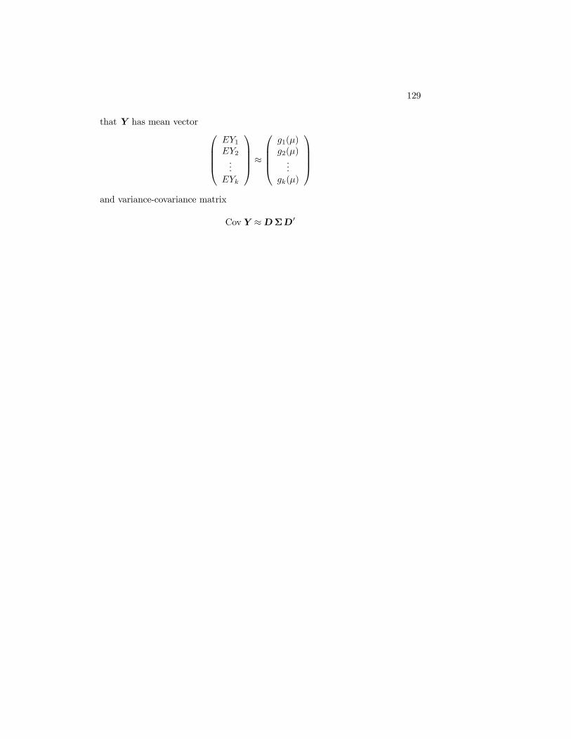
129
that Y has mean vector0BBB@
EY1EY2
...EYk
1CCCA ¼
0BBB@
g1(¹)g2(¹)
...gk(¹)
1CCCA
and variance-covariance matrix
CovY ¼ D §D0