gradient-based learning applied to document recognition · gradient-based learning applied to...

Gradient-Based Learning Appliedto Document Recognition

YANN LECUN, MEMBER, IEEE,LEON BOTTOU, YOSHUA BENGIO,AND PATRICK HAFFNER

Invited Paper

Multilayer neural networks trained with the back-propagationalgorithm constitute the best example of a successful gradient-based learning technique. Given an appropriate networkarchitecture, gradient-based learning algorithms can be usedto synthesize a complex decision surface that can classifyhigh-dimensional patterns, such as handwritten characters, withminimal preprocessing. This paper reviews various methodsapplied to handwritten character recognition and compares themon a standard handwritten digit recognition task. Convolutionalneural networks, which are specifically designed to deal withthe variability of two dimensional (2-D) shapes, are shown tooutperform all other techniques.

Real-life document recognition systems are composed of multiplemodules including field extraction, segmentation, recognition,and language modeling. A new learning paradigm, called graphtransformer networks (GTN’s), allows such multimodule systemsto be trained globally using gradient-based methods so as tominimize an overall performance measure.

Two systems for online handwriting recognition are described.Experiments demonstrate the advantage of global training, andthe flexibility of graph transformer networks.

A graph transformer network for reading a bank check isalso described. It uses convolutional neural network characterrecognizers combined with global training techniques to providerecord accuracy on business and personal checks. It is deployedcommercially and reads several million checks per day.

Keywords—Convolutional neural networks, document recog-nition, finite state transducers, gradient-based learning, graphtransformer networks, machine learning, neural networks, opticalcharacter recognition (OCR).

NOMENCLATURE

GT Graph transformer.GTN Graph transformer network.HMM Hidden Markov model.HOS Heuristic oversegmentation.K-NN K-nearest neighbor.

Manuscript received November 1, 1997; revised April 17, 1998.Y. LeCun, L. Bottou, and P. Haffner are with the Speech and Image

Processing Services Research Laboratory, AT&T Labs-Research, RedBank, NJ 07701 USA.

Y. Bengio is with the Departement d’Informatique et de RechercheOperationelle, Universite de Montreal, Montreal, Quebec H3C 3J7 Canada.

Publisher Item Identifier S 0018-9219(98)07863-3.

NN Neural network.OCR Optical character recognition.PCA Principal component analysis.RBF Radial basis function.RS-SVM Reduced-set support vector method.SDNN Space displacement neural network.SVM Support vector method.TDNN Time delay neural network.V-SVM Virtual support vector method.

I. INTRODUCTION

Over the last several years, machine learning techniques,particularly when applied to NN’s, have played an increas-ingly important role in the design of pattern recognitionsystems. In fact, it could be argued that the availabilityof learning techniques has been a crucial factor in therecent success of pattern recognition applications such ascontinuous speech recognition and handwriting recognition.

The main message of this paper is that better patternrecognition systems can be built by relying more on auto-matic learning and less on hand-designed heuristics. Thisis made possible by recent progress in machine learningand computer technology. Using character recognition as acase study, we show that hand-crafted feature extraction canbe advantageously replaced by carefully designed learningmachines that operate directly on pixel images. Usingdocument understanding as a case study, we show that thetraditional way of building recognition systems by manuallyintegrating individually designed modules can be replacedby a unified and well-principled design paradigm, calledGTN’s, which allows training all the modules to optimizea global performance criterion.

Since the early days of pattern recognition it has beenknown that the variability and richness of natural data,be it speech, glyphs, or other types of patterns, make italmost impossible to build an accurate recognition systementirely by hand. Consequently, most pattern recognitionsystems are built using a combination of automatic learningtechniques and hand-crafted algorithms. The usual method

0018–9219/98$10.00 1998 IEEE

2278 PROCEEDINGS OF THE IEEE, VOL. 86, NO. 11, NOVEMBER 1998

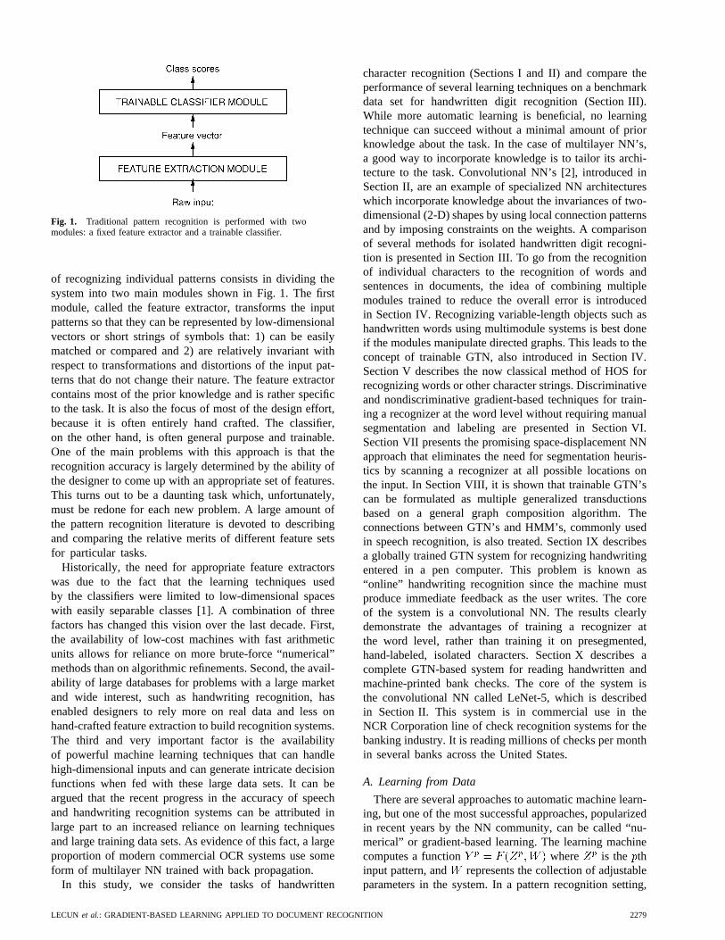
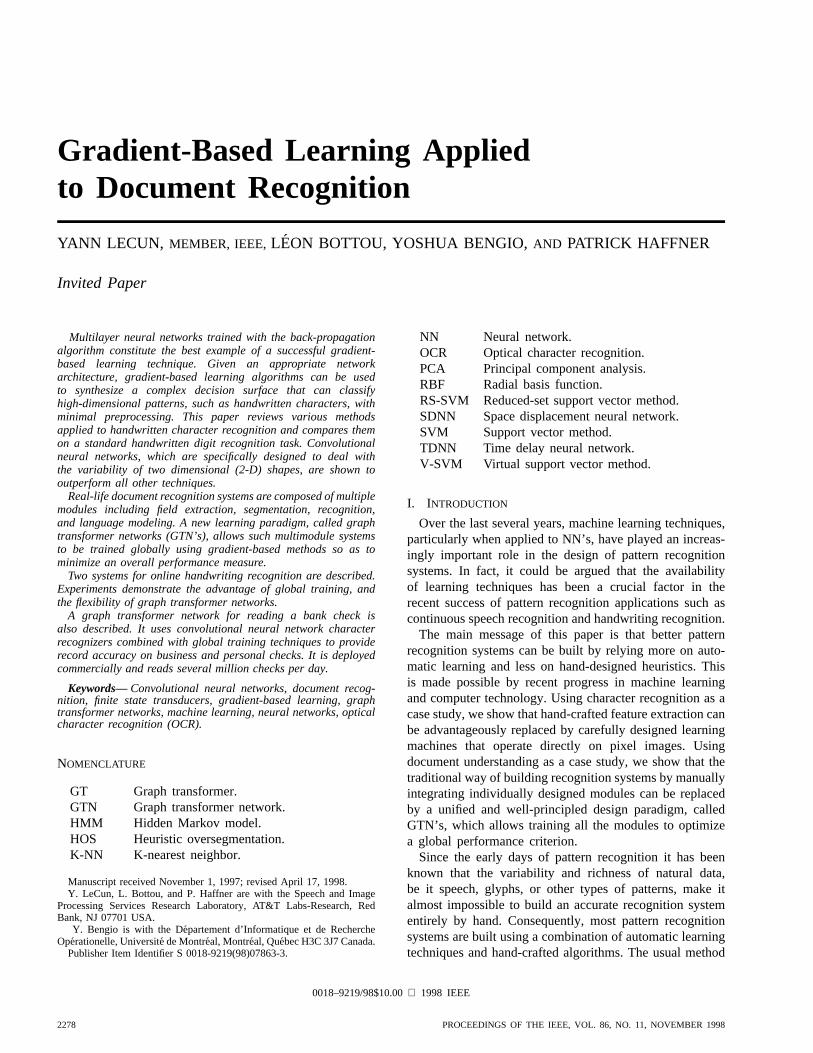
Fig. 1. Traditional pattern recognition is performed with twomodules: a fixed feature extractor and a trainable classifier.

of recognizing individual patterns consists in dividing thesystem into two main modules shown in Fig. 1. The firstmodule, called the feature extractor, transforms the inputpatterns so that they can be represented by low-dimensionalvectors or short strings of symbols that: 1) can be easilymatched or compared and 2) are relatively invariant withrespect to transformations and distortions of the input pat-terns that do not change their nature. The feature extractorcontains most of the prior knowledge and is rather specificto the task. It is also the focus of most of the design effort,because it is often entirely hand crafted. The classifier,on the other hand, is often general purpose and trainable.One of the main problems with this approach is that therecognition accuracy is largely determined by the ability ofthe designer to come up with an appropriate set of features.This turns out to be a daunting task which, unfortunately,must be redone for each new problem. A large amount ofthe pattern recognition literature is devoted to describingand comparing the relative merits of different feature setsfor particular tasks.

Historically, the need for appropriate feature extractorswas due to the fact that the learning techniques usedby the classifiers were limited to low-dimensional spaceswith easily separable classes [1]. A combination of threefactors has changed this vision over the last decade. First,the availability of low-cost machines with fast arithmeticunits allows for reliance on more brute-force “numerical”methods than on algorithmic refinements. Second, the avail-ability of large databases for problems with a large marketand wide interest, such as handwriting recognition, hasenabled designers to rely more on real data and less onhand-crafted feature extraction to build recognition systems.The third and very important factor is the availabilityof powerful machine learning techniques that can handlehigh-dimensional inputs and can generate intricate decisionfunctions when fed with these large data sets. It can beargued that the recent progress in the accuracy of speechand handwriting recognition systems can be attributed inlarge part to an increased reliance on learning techniquesand large training data sets. As evidence of this fact, a largeproportion of modern commercial OCR systems use someform of multilayer NN trained with back propagation.

In this study, we consider the tasks of handwritten

character recognition (Sections I and II) and compare theperformance of several learning techniques on a benchmarkdata set for handwritten digit recognition (Section III).While more automatic learning is beneficial, no learningtechnique can succeed without a minimal amount of priorknowledge about the task. In the case of multilayer NN’s,a good way to incorporate knowledge is to tailor its archi-tecture to the task. Convolutional NN’s [2], introduced inSection II, are an example of specialized NN architectureswhich incorporate knowledge about the invariances of two-dimensional (2-D) shapes by using local connection patternsand by imposing constraints on the weights. A comparisonof several methods for isolated handwritten digit recogni-tion is presented in Section III. To go from the recognitionof individual characters to the recognition of words andsentences in documents, the idea of combining multiplemodules trained to reduce the overall error is introducedin Section IV. Recognizing variable-length objects such ashandwritten words using multimodule systems is best doneif the modules manipulate directed graphs. This leads to theconcept of trainable GTN, also introduced in Section IV.Section V describes the now classical method of HOS forrecognizing words or other character strings. Discriminativeand nondiscriminative gradient-based techniques for train-ing a recognizer at the word level without requiring manualsegmentation and labeling are presented in Section VI.Section VII presents the promising space-displacement NNapproach that eliminates the need for segmentation heuris-tics by scanning a recognizer at all possible locations onthe input. In Section VIII, it is shown that trainable GTN’scan be formulated as multiple generalized transductionsbased on a general graph composition algorithm. Theconnections between GTN’s and HMM’s, commonly usedin speech recognition, is also treated. Section IX describesa globally trained GTN system for recognizing handwritingentered in a pen computer. This problem is known as“online” handwriting recognition since the machine mustproduce immediate feedback as the user writes. The coreof the system is a convolutional NN. The results clearlydemonstrate the advantages of training a recognizer atthe word level, rather than training it on presegmented,hand-labeled, isolated characters. Section X describes acomplete GTN-based system for reading handwritten andmachine-printed bank checks. The core of the system isthe convolutional NN called LeNet-5, which is describedin Section II. This system is in commercial use in theNCR Corporation line of check recognition systems for thebanking industry. It is reading millions of checks per monthin several banks across the United States.

A. Learning from Data

There are several approaches to automatic machine learn-ing, but one of the most successful approaches, popularizedin recent years by the NN community, can be called “nu-merical” or gradient-based learning. The learning machinecomputes a function where is the thinput pattern, and represents the collection of adjustableparameters in the system. In a pattern recognition setting,

LECUN et al.: GRADIENT-BASED LEARNING APPLIED TO DOCUMENT RECOGNITION 2279

the output may be interpreted as the recognized classlabel of pattern or as scores or probabilities associatedwith each class. A loss functionmeasures the discrepancy between the “correct” ordesired output for pattern and the output produced bythe system. The average loss function is theaverage of the errors over a set of labeled examplescalled the training set In thesimplest setting, the learning problem consists in findingthe value of that minimizes In practice,the performance of the system on a training set is of littleinterest. The more relevant measure is the error rate of thesystem in the field, where it would be used in practice.This performance is estimated by measuring the accuracyon a set of samples disjoint from the training set, which iscalled the test set. Much theoretical and experimental work[3]–[5] has shown that the gap between the expected errorrate on the test set and the error rate on the trainingset decreases with the number of training samplesapproximately as

(1)

where is the number of training samples,is a measureof “effective capacity” or complexity of the machine [6],[7], is a number between 0.5 and 1.0, andis a constant.This gap always decreases when the number of trainingsamples increases. Furthermore, as the capacityincreases,

decreases. Therefore, when increasing the capacitythere is a tradeoff between the decrease of and the

increase of the gap, with an optimal value of the capacitythat achieves the lowest generalization error Most

learning algorithms attempt to minimize as well assome estimate of the gap. A formal version of this is calledstructural risk minimization [6], [7], and it is based on defin-ing a sequence of learning machines of increasing capacity,corresponding to a sequence of subsets of the parameterspace such that each subset is a superset of the previoussubset. In practical terms, structural risk minimization isimplemented by minimizing where thefunction is called a regularization function andisa constant. is chosen such that it takes large valueson parameters that belong to high-capacity subsets ofthe parameter space. Minimizing in effect limits thecapacity of the accessible subset of the parameter space,thereby controlling the tradeoff between minimizing thetraining error and minimizing the expected gap betweenthe training error and test error.

B. Gradient-Based Learning

The general problem of minimizing a function withrespect to a set of parameters is at the root of manyissues in computer science. Gradient-based learning drawson the fact that it is generally much easier to minimizea reasonably smooth, continuous function than a discrete(combinatorial) function. The loss function can be mini-mized by estimating the impact of small variations of theparameter values on the loss function. This is measured

by the gradient of the loss function with respect to theparameters. Efficient learning algorithms can be devisedwhen the gradient vector can be computed analytically (asopposed to numerically through perturbations). This is thebasis of numerous gradient-based learning algorithms withcontinuous-valued parameters. In the procedures describedin this article, the set of parameters is a real-valuedvector, with respect to which is continuous, as wellas differentiable almost everywhere. The simplest mini-mization procedure in such a setting is the gradient descentalgorithm where is iteratively adjusted as follows:

(2)

In the simplest case, is a scalar constant. More sophis-ticated procedures use variable or substitute it for adiagonal matrix, or substitute it for an estimate of theinverse Hessian matrix as in Newton or quasi-Newtonmethods. The conjugate gradient method [8] can also beused. However, Appendix B shows that despite manyclaims to the contrary in the literature, the usefulness ofthese second-order methods to large learning machines isvery limited.

A popular minimization procedure is the stochastic gra-dient algorithm, also called the online update. It consistsin updating the parameter vector using a noisy, or approxi-mated, version of the average gradient. In the most commoninstance of it, is updated on the basis of a single sample

(3)

With this procedure the parameter vector fluctuates aroundan average trajectory, but usually it converges considerablyfaster than regular gradient descent and second-order meth-ods on large training sets with redundant samples (suchas those encountered in speech or character recognition).The reasons for this are explained in Appendix B. Theproperties of such algorithms applied to learning have beenstudied theoretically since the 1960’s [9]–[11], but practicalsuccesses for nontrivial tasks did not occur until the mideighties.

C. Gradient Back Propagation

Gradient-based learning procedures have been used sincethe late 1950’s, but they were mostly limited to linearsystems [1]. The surprising usefulness of such simplegradient descent techniques for complex machine learningtasks was not widely realized until the following threeevents occurred. The first event was the realization that,despite early warnings to the contrary [12], the presence oflocal minima in the loss function does not seem to be amajor problem in practice. This became apparent when itwas noticed that local minima did not seem to be a majorimpediment to the success of early nonlinear gradient-basedlearning techniques such as Boltzmann machines [13], [14].The second event was the popularization by Rumelhartetal. [15] and others of a simple and efficient procedureto compute the gradient in a nonlinear system composed


of several layers of processing, i.e., the back-propagationalgorithm. The third event was the demonstration that theback-propagation procedure applied to multilayer NN’swith sigmoidal units can solve complicated learning tasks.The basic idea of back propagation is that gradients canbe computed efficiently by propagation from the output tothe input. This idea was described in the control theoryliterature of the early 1960’s [16], but its application to ma-chine learning was not generally realized then. Interestingly,the early derivations of back propagation in the contextof NN learning did not use gradients but “virtual targets”for units in intermediate layers [17], [18], or minimaldisturbance arguments [19]. The Lagrange formalism usedin the control theory literature provides perhaps the bestrigorous method for deriving back propagation [20] and forderiving generalizations of back propagation to recurrentnetworks [21] and networks of heterogeneous modules [22].A simple derivation for generic multilayer systems is givenin Section I-E.

The fact that local minima do not seem to be a problemfor multilayer NN’s is somewhat of a theoretical mystery.It is conjectured that if the network is oversized for thetask (as is usually the case in practice), the presence of“extra dimensions” in parameter space reduces the riskof unattainable regions. Back propagation is by far themost widely used neural-network learning algorithm, andprobably the most widely used learning algorithm of anyform.

D. Learning in Real Handwriting Recognition Systems

Isolated handwritten character recognition has been ex-tensively studied in the literature (see [23] and [24] forreviews), and it was one of the early successful applicationsof NN’s [25]. Comparative experiments on recognition ofindividual handwritten digits are reported in Section III.They show that NN’s trained with gradient-based learningperform better than all other methods tested here on thesame data. The best NN’s, called convolutional networks,are designed to learn to extract relevant features directlyfrom pixel images (see Section II).

One of the most difficult problems in handwriting recog-nition, however, is not only to recognize individual charac-ters, but also to separate out characters from their neighborswithin the word or sentence, a process known as seg-mentation. The technique for doing this that has becomethe “standard” is called HOS. It consists of generating alarge number of potential cuts between characters usingheuristic image processing techniques, and subsequentlyselecting the best combination of cuts based on scoresgiven for each candidate character by the recognizer. Insuch a model, the accuracy of the system depends upon thequality of the cuts generated by the heuristics, and on theability of the recognizer to distinguish correctly segmentedcharacters from pieces of characters, multiple characters,or otherwise incorrectly segmented characters. Training arecognizer to perform this task poses a major challengebecause of the difficulty in creating a labeled databaseof incorrectly segmented characters. The simplest solution

consists of running the images of character strings throughthe segmenter and then manually labeling all the characterhypotheses. Unfortunately, not only is this an extremelytedious and costly task, it is also difficult to do the labelingconsistently. For example, should the right half of a cut-upfour be labeled as a one or as a noncharacter? Should theright half of a cut-up eight be labeled as a three?

The first solution, described in Section V, consists oftraining the system at the level of whole strings of char-acters rather than at the character level. The notion ofgradient-based learning can be used for this purpose. Thesystem is trained to minimize an overall loss function whichmeasures the probability of an erroneous answer. Section Vexplores various ways to ensure that the loss functionis differentiable and therefore lends itself to the use ofgradient-based learning methods. Section V introduces theuse of directed acyclic graphs whose arcs carry numericalinformation as a way to represent the alternative hypothesesand introduces the idea of GTN.

The second solution, described in Section VII, is toeliminate segmentation altogether. The idea is to sweepthe recognizer over every possible location on the inputimage, and to rely on the “character spotting” propertyof the recognizer, i.e., its ability to correctly recognizea well-centered character in its input field, even in thepresence of other characters besides it, while rejectingimages containing no centered characters [26], [27]. Thesequence of recognizer outputs obtained by sweeping therecognizer over the input is then fed to a GTN that takeslinguistic constraints into account and finally extracts themost likely interpretation. This GTN is somewhat similarto HMM’s, which makes the approach reminiscent of theclassical speech recognition [28], [29]. While this techniquewould be quite expensive in the general case, the use ofconvolutional NN’s makes it particularly attractive becauseit allows significant savings in computational cost.

E. Globally Trainable Systems

As stated earlier, most practical pattern recognition sys-tems are composed of multiple modules. For example, adocument recognition system is composed of a field loca-tor (which extracts regions of interest), a field segmenter(which cuts the input image into images of candidatecharacters), a recognizer (which classifies and scores eachcandidate character), and a contextual postprocessor, gen-erally based on a stochastic grammar (which selects thebest grammatically correct answer from the hypothesesgenerated by the recognizer). In most cases, the informationcarried from module to module is best represented asgraphs with numerical information attached to the arcs.For example, the output of the recognizer module can berepresented as an acyclic graph where each arc contains thelabel and the score of a candidate character, and where eachpath represents an alternative interpretation of the inputstring. Typically, each module is manually optimized, orsometimes trained, outside of its context. For example, thecharacter recognizer would be trained on labeled imagesof presegmented characters. Then the complete system is


assembled, and a subset of the parameters of the modulesis manually adjusted to maximize the overall performance.This last step is extremely tedious, time consuming, andalmost certainly suboptimal.

A better alternative would be to somehow train the entiresystem so as to minimize a global error measure suchas the probability of character misclassifications at thedocument level. Ideally, we would want to find a goodminimum of this global loss function with respect to all theparameters in the system. If the loss functionmeasuringthe performance can be made differentiable with respectto the system’s tunable parameters we can find a localminimum of using gradient-based learning. However, atfirst glance, it appears that the sheer size and complexityof the system would make this intractable.

To ensure that the global loss function isdifferentiable, the overall system is built as a feedforwardnetwork of differentiable modules. The function imple-mented by each module must be continuous and differ-entiable almost everywhere with respect to the internalparameters of the module (e.g., the weights of an NNcharacter recognizer in the case of a character recognitionmodule), and with respect to the module’s inputs. If this isthe case, a simple generalization of the well-known back-propagation procedure can be used to efficiently computethe gradients of the loss function with respect to all theparameters in the system [22]. For example, let us considera system built as a cascade of modules, each of whichimplements a function whereis a vector representing the output of the module, isthe vector of tunable parameters in the module (a subset of

and is the module’s input vector (as well as theprevious module’s output vector). The input to the firstmodule is the input pattern If the partial derivative of

with respect to is known, then the partial derivativesof with respect to and can be computed usingthe backward recurrence

(4)

where is the Jacobian of withrespect to evaluated at the point and

is the Jacobian of with respect toThe Jacobian of a vector function is a matrix containing

the partial derivatives of all the outputs with respect toall the inputs. The first equation computes some termsof the gradient of while the second equationgenerates a backward recurrence, as in the well-knownback-propagation procedure for NN’s. We can averagethe gradients over the training patterns to obtain the fullgradient. It is interesting to note that in many instancesthere is no need to explicitly compute the Jacobian ma-trix. The above formula uses the product of the Jacobianwith a vector of partial derivatives, and it is often easierto compute this product directly without computing theJacobian beforehand. In analogy with ordinary multilayer

NN’s, all but the last module are called hidden layersbecause their outputs are not observable from the outside.In more complex situations than the simple cascade ofmodules described above, the partial derivative notationbecomes somewhat ambiguous and awkward. A completelyrigorous derivation in more general cases can be done usingLagrange functions [20]–[22].

Traditional multilayer NN’s are a special case of theabove where the state information is representedwith fixed-sized vectors, and where the modules arealternated layers of matrix multiplications (the weights)and component-wise sigmoid functions (the neurons).However, as stated earlier, the state information in complexrecognition system is best represented by graphs withnumerical information attached to the arcs. In this case,each module, called a GT, takes one or more graphs as inputand produces a graph as output. Networks of such modulesare called GTN’s. Sections IV, VI, and VIII develop theconcept of GTN’s and show that gradient-based learningcan be used to train all the parameters in all the modulesso as to minimize a global loss function. It may seemparadoxical that gradients can be computed when the stateinformation is represented by essentially discrete objectssuch as graphs, but that difficulty can be circumvented,as shown later.

II. CONVOLUTIONAL NEURAL NETWORKS FOR

ISOLATED CHARACTER RECOGNITION

The ability of multilayer networks trained with gradi-ent descent to learn complex, high-dimensional, nonlinearmappings from large collections of examples makes themobvious candidates for image recognition tasks. In thetraditional model of pattern recognition, a hand-designedfeature extractor gathers relevant information from the inputand eliminates irrelevant variabilities. A trainable classifierthen categorizes the resulting feature vectors into classes. Inthis scheme, standard, fully connected multilayer networkscan be used as classifiers. A potentially more interestingscheme is to rely as much as possible on learning in thefeature extractor itself. In the case of character recognition,a network could be fed with almost raw inputs (e.g.,size-normalized images). While this can be done with anordinary fully connected feedforward network with somesuccess for tasks such as character recognition, there areproblems.

First, typical images are large, often with several hundredvariables (pixels). A fully connected first layer with, e.g.,one hundred hidden units in the first layer would alreadycontain several tens of thousands of weights. Such a largenumber of parameters increases the capacity of the systemand therefore requires a larger training set. In addition, thememory requirement to store so many weights may rule outcertain hardware implementations. But the main deficiencyof unstructured nets for image or speech applications is thatthey have no built-in invariance with respect to translationsor local distortions of the inputs. Before being sent tothe fixed-size input layer of an NN, character images,


Fig. 2. Architecture of LeNet-5, a convolutional NN, here used for digits recognition. Each planeis a feature map, i.e., a set of units whose weights are constrained to be identical.

or other 2-D or one-dimensional (1-D) signals, must beapproximately size normalized and centered in the inputfield. Unfortunately, no such preprocessing can be perfect:handwriting is often normalized at the word level, whichcan cause size, slant, and position variations for individualcharacters. This, combined with variability in writing style,will cause variations in the position of distinctive featuresin input objects. In principle, a fully connected network ofsufficient size could learn to produce outputs that are invari-ant with respect to such variations. However, learning sucha task would probably result in multiple units with similarweight patterns positioned at various locations in the inputso as to detect distinctive features wherever they appear onthe input. Learning these weight configurations requires avery large number of training instances to cover the space ofpossible variations. In convolutional networks, as describedbelow, shift invariance is automatically obtained by forcingthe replication of weight configurations across space.

Secondly, a deficiency of fully connected architectures isthat the topology of the input is entirely ignored. The inputvariables can be presented in any (fixed) order without af-fecting the outcome of the training. On the contrary, images(or time-frequency representations of speech) have a strong2-D local structure: variables (or pixels) that are spatially ortemporally nearby are highly correlated. Local correlationsare the reasons for the well-known advantages of extractingand combining local features before recognizing spatialor temporal objects, because configurations of neighboringvariables can be classified into a small number of categories(e.g., edges, corners, etc.). Convolutional networks forcethe extraction of local features by restricting the receptivefields of hidden units to be local.

A. Convolutional Networks

Convolutional networks combine three architectural ideasto ensure some degree of shift, scale, and distortion in-variance: 1) local receptive fields; 2) shared weights (orweight replication); and 3) spatial or temporal subsampling.A typical convolutional network for recognizing characters,dubbed LeNet-5, is shown in Fig. 2. The input planereceives images of characters that are approximately sizenormalized and centered. Each unit in a layer receivesinputs from a set of units located in a small neighborhood

in the previous layer. The idea of connecting units to localreceptive fields on the input goes back to the perceptron inthe early 1960’s, and it was almost simultaneous with Hubeland Wiesel’s discovery of locally sensitive, orientation-selective neurons in the cat’s visual system [30]. Localconnections have been used many times in neural modelsof visual learning [2], [18], [31]–[34]. With local receptivefields neurons can extract elementary visual features suchas oriented edges, endpoints, corners (or similar features inother signals such as speech spectrograms). These featuresare then combined by the subsequent layers in order todetect higher order features. As stated earlier, distortions orshifts of the input can cause the position of salient featuresto vary. In addition, elementary feature detectors that areuseful on one part of the image are likely to be useful acrossthe entire image. This knowledge can be applied by forcinga set of units, whose receptive fields are located at differentplaces on the image, to have identical weight vectors [15],[32], [34]. Units in a layer are organized in planes withinwhich all the units share the same set of weights. The set ofoutputs of the units in such a plane is called a feature map.Units in a feature map are all constrained to perform thesame operation on different parts of the image. A completeconvolutional layer is composed of several feature maps(with different weight vectors), so that multiple featurescan be extracted at each location. A concrete example ofthis is the first layer of LeNet-5 shown in Fig. 2. Unitsin the first hidden layer of LeNet-5 are organized in sixplanes, each of which is a feature map. A unit in a featuremap has 25 inputs connected to a 55 area in the input,called the receptive field of the unit. Each unit has 25inputs and therefore 25 trainable coefficients plus a trainablebias. The receptive fields of contiguous units in a featuremap are centered on corresponding contiguous units in theprevious layer. Therefore, receptive fields of neighboringunits overlap. For example, in the first hidden layer ofLeNet-5, the receptive fields of horizontally contiguousunits overlap by four columns and five rows. As statedearlier, all the units in a feature map share the same set of 25weights and the same bias, so they detect the same featureat all possible locations on the input. The other featuremaps in the layer use different sets of weights and biases,thereby extracting different types of local features. In the


case of LeNet-5, at each input location six different typesof features are extracted by six units in identical locationsin the six feature maps. A sequential implementation ofa feature map would scan the input image with a singleunit that has a local receptive field and store the statesof this unit at corresponding locations in the feature map.This operation is equivalent to a convolution, followed byan additive bias and squashing function, hence the nameconvolutional network. The kernel of the convolution is theset of connection weights used by the units in the featuremap. An interesting property of convolutional layers is thatif the input image is shifted, the feature map output will beshifted by the same amount, but it will be left unchangedotherwise. This property is at the basis of the robustness ofconvolutional networks to shifts and distortions of the input.

Once a feature has been detected, its exact locationbecomes less important. Only its approximate positionrelative to other features is relevant. For example, oncewe know that the input image contains the endpoint of aroughly horizontal segment in the upper left area, a cornerin the upper right area, and the endpoint of a roughlyvertical segment in the lower portion of the image, we cantell the input image is a seven. Not only is the preciseposition of each of those features irrelevant for identifyingthe pattern, it is potentially harmful because the positionsare likely to vary for different instances of the character. Asimple way to reduce the precision with which the positionof distinctive features are encoded in a feature map isto reduce the spatial resolution of the feature map. Thiscan be achieved with a so-called subsampling layer, whichperforms a local averaging and a subsampling, therebyreducing the resolution of the feature map and reducingthe sensitivity of the output to shifts and distortions. Thesecond hidden layer of LeNet-5 is a subsampling layer. Thislayer comprises six feature maps, one for each feature mapin the previous layer. The receptive field of each unit isa 2 2 area in the previous layer’s corresponding featuremap. Each unit computes the average of its four inputs,multiplies it by a trainable coefficient, adds a trainablebias, and passes the result through a sigmoid function.Contiguous units have nonoverlapping contiguous receptivefields. Consequently, a subsampling layer feature map hashalf the number of rows and columns as the feature maps inthe previous layer. The trainable coefficient and bias controlthe effect of the sigmoid nonlinearity. If the coefficient issmall, then the unit operates in a quasi-linear mode, and thesubsampling layer merely blurs the input. If the coefficientis large, subsampling units can be seen as performing a“noisy OR” or a “noisy AND” function depending onthe value of the bias. Successive layers of convolutionsand subsampling are typically alternated resulting in a“bipyramid”: at each layer, the number of feature mapsis increased as the spatial resolution is decreased. Eachunit in the third hidden layer in Fig. 2 may have inputconnections from several feature maps in the previouslayer. The convolution/subsampling combination, inspiredby Hubel and Wiesel’s notions of “simple” and “complex”cells, was implemented in Fukushima’s Neocognitron [32],

though no globally supervised learning procedure suchas back propagation was available then. A large degreeof invariance to geometric transformations of the inputcan be achieved with this progressive reduction of spatialresolution compensated by a progressive increase of therichness of the representation (the number of feature maps).

Since all the weights are learned with back propagation,convolutional networks can be seen as synthesizing theirown feature extractor. The weight sharing technique hasthe interesting side effect of reducing the number of freeparameters, thereby reducing the “capacity” of the machineand reducing the gap between test error and training error[34]. The network in Fig. 2 contains 345 308 connections,but only 60 000 trainable free parameters because of theweight sharing.

Fixed-size convolutional networks have been applied tomany applications, among other handwriting recognition[35], [36], machine-printed character recognition [37], on-line handwriting recognition [38], and face recognition[39]. Fixed-size convolutional networks that share weightsalong a single temporal dimension are known as time-delayNN’s (TDNN’s). TDNN’s have been used in phonemerecognition (without subsampling) [40], [41], spoken wordrecognition (with subsampling) [42], [43], online recogni-tion of isolated handwritten characters [44], and signatureverification [45].

B. LeNet-5

This section describes in more detail the architecture ofLeNet-5, the Convolutional NN used in the experiments.LeNet-5 comprises seven layers, not counting the input, allof which contain trainable parameters (weights). The inputis a 32 32 pixel image. This is significantly larger thanthe largest character in the database (at most 2020 pixelscentered in a 2828 field). The reason is that it is desirablethat potential distinctive features such as stroke endpointsor corner can appear in the center of the receptive fieldof the highest level feature detectors. In LeNet-5, the setof centers of the receptive fields of the last convolutionallayer (C3, see below) form a 2020 area in the center of the32 32 input. The values of the input pixels are normalizedso that the background level (white) corresponds to a valueof and the foreground (black) corresponds to 1.175.This makes the mean input roughly zero and the varianceroughly one, which accelerates learning [46].

In the following, convolutional layers are labeled Cx,subsampling layers are labeled Sx, and fully connectedlayers are labeled Fx, where x is the layer index.

Layer C1 is a convolutional layer with six feature maps.Each unit in each feature map is connected to a 55 neigh-borhood in the input. The size of the feature maps is 2828which prevents connection from the input from falling offthe boundary. C1 contains 156 trainable parameters and122 304 connections.

Layer S2 is a subsampling layer with six feature maps ofsize 14 14. Each unit in each feature map is connected to a2 2 neighborhood in the corresponding feature map in C1.The four inputs to a unit in S2 are added, then multiplied by


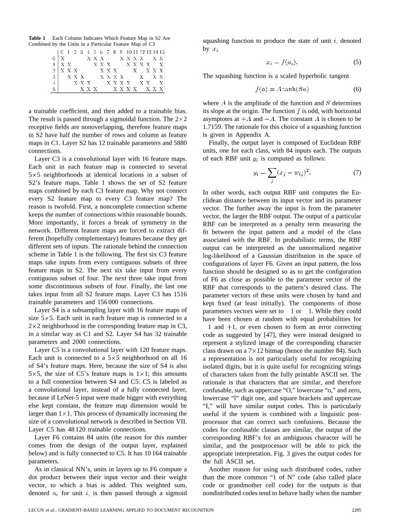
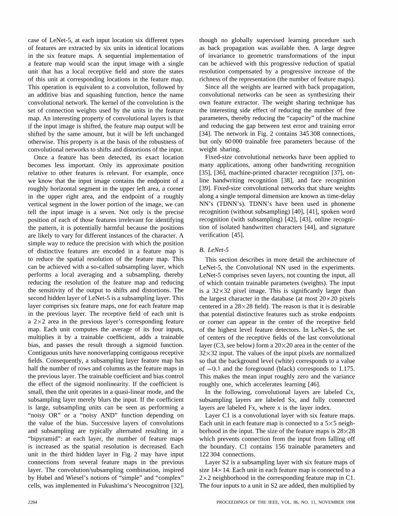
Table 1 Each Column Indicates Which Feature Map in S2 AreCombined by the Units in a Particular Feature Map of C3

a trainable coefficient, and then added to a trainable bias.The result is passed through a sigmoidal function. The 22receptive fields are nonoverlapping, therefore feature mapsin S2 have half the number of rows and column as featuremaps in C1. Layer S2 has 12 trainable parameters and 5880connections.

Layer C3 is a convolutional layer with 16 feature maps.Each unit in each feature map is connected to several5 5 neighborhoods at identical locations in a subset ofS2’s feature maps. Table 1 shows the set of S2 featuremaps combined by each C3 feature map. Why not connectevery S2 feature map to every C3 feature map? Thereason is twofold. First, a noncomplete connection schemekeeps the number of connections within reasonable bounds.More importantly, it forces a break of symmetry in thenetwork. Different feature maps are forced to extract dif-ferent (hopefully complementary) features because they getdifferent sets of inputs. The rationale behind the connectionscheme in Table 1 is the following. The first six C3 featuremaps take inputs from every contiguous subsets of threefeature maps in S2. The next six take input from everycontiguous subset of four. The next three take input fromsome discontinuous subsets of four. Finally, the last onetakes input from all S2 feature maps. Layer C3 has 1516trainable parameters and 156 000 connections.

Layer S4 is a subsampling layer with 16 feature maps ofsize 5 5. Each unit in each feature map is connected to a2 2 neighborhood in the corresponding feature map in C3,in a similar way as C1 and S2. Layer S4 has 32 trainableparameters and 2000 connections.

Layer C5 is a convolutional layer with 120 feature maps.Each unit is connected to a 55 neighborhood on all 16of S4’s feature maps. Here, because the size of S4 is also5 5, the size of C5’s feature maps is 11; this amountsto a full connection between S4 and C5. C5 is labeled asa convolutional layer, instead of a fully connected layer,because if LeNet-5 input were made bigger with everythingelse kept constant, the feature map dimension would belarger than 1 1. This process of dynamically increasing thesize of a convolutional network is described in Section VII.Layer C5 has 48 120 trainable connections.

Layer F6 contains 84 units (the reason for this numbercomes from the design of the output layer, explainedbelow) and is fully connected to C5. It has 10 164 trainableparameters.

As in classical NN’s, units in layers up to F6 compute adot product between their input vector and their weightvector, to which a bias is added. This weighted sum,denoted for unit is then passed through a sigmoid

squashing function to produce the state of unitdenotedby

(5)

The squashing function is a scaled hyperbolic tangent

(6)

where is the amplitude of the function and determinesits slope at the origin. The functionis odd, with horizontalasymptotes at and The constant is chosen to be1.7159. The rationale for this choice of a squashing functionis given in Appendix A.

Finally, the output layer is composed of Euclidean RBFunits, one for each class, with 84 inputs each. The outputsof each RBF unit is computed as follows:

(7)

In other words, each output RBF unit computes the Eu-clidean distance between its input vector and its parametervector. The further away the input is from the parametervector, the larger the RBF output. The output of a particularRBF can be interpreted as a penalty term measuring thefit between the input pattern and a model of the classassociated with the RBF. In probabilistic terms, the RBFoutput can be interpreted as the unnormalized negativelog-likelihood of a Gaussian distribution in the space ofconfigurations of layer F6. Given an input pattern, the lossfunction should be designed so as to get the configurationof F6 as close as possible to the parameter vector of theRBF that corresponds to the pattern’s desired class. Theparameter vectors of these units were chosen by hand andkept fixed (at least initially). The components of thoseparameters vectors were set to1 or 1. While they couldhave been chosen at random with equal probabilities for

1 and 1, or even chosen to form an error correctingcode as suggested by [47], they were instead designed torepresent a stylized image of the corresponding characterclass drawn on a 712 bitmap (hence the number 84). Sucha representation is not particularly useful for recognizingisolated digits, but it is quite useful for recognizing stringsof characters taken from the fully printable ASCII set. Therationale is that characters that are similar, and thereforeconfusable, such as uppercase “O,” lowercase “o,” and zero,lowercase “l” digit one, and square brackets and uppercase“I,” will have similar output codes. This is particularlyuseful if the system is combined with a linguistic post-processor that can correct such confusions. Because thecodes for confusable classes are similar, the output of thecorresponding RBF’s for an ambiguous character will besimilar, and the postprocessor will be able to pick theappropriate interpretation. Fig. 3 gives the output codes forthe full ASCII set.

Another reason for using such distributed codes, ratherthan the more common “1 of N” code (also called placecode or grandmother cell code) for the outputs is thatnondistributed codes tend to behave badly when the number


Fig. 3. Initial parameters of the output RBF’s for recognizing the full ASCII set.

of classes is larger than a few dozen. The reason isthat output units in a nondistributed code must be offmost of the time. This is quite difficult to achieve withsigmoid units. Yet another reason is that the classifiers areoften used not only to recognize characters, but also toreject noncharacters. RBF’s with distributed codes are moreappropriate for that purpose because unlike sigmoids, theyare activated within a well-circumscribed region of theirinput space, outside of which nontypical patterns are morelikely to fall.

The parameter vectors of the RBF’s play the role oftarget vectors for layer F6. It is worth pointing out thatthe components of those vectors are1 or 1, which iswell within the range of the sigmoid of F6, and thereforeprevents those sigmoids from getting saturated. In fact,

1 and 1 are the points of maximum curvature of thesigmoids. This forces the F6 units to operate in theirmaximally nonlinear range. Saturation of the sigmoids mustbe avoided because it is known to lead to slow convergenceand ill-conditioning of the loss function.

C. Loss Function

The simplest output loss function that can be used withthe above network is the maximum likelihood estimationcriterion, which in our case is equivalent to the minimummean squared error (MSE). The criterion for a set oftraining samples is simply

(8)

where is the output of the th RBF unit, i.e., theone that corresponds to the correct class of input pattern

While this cost function is appropriate for most cases,it lacks three important properties. First, if we allow theparameters of the RBF to adapt, has a trivial, buttotally unacceptable, solution. In this solution, all the RBFparameter vectors are equal and the state of F6 is constantand equal to that parameter vector. In this case the networkhappily ignores the input, and all the RBF outputs are equal

to zero. This collapsing phenomenon does not occur if theRBF weights are not allowed to adapt. The second problemis that there is no competition between the classes. Such acompetition can be obtained by using a more discriminativetraining criterion, dubbed the maximuma posteriori(MAP)criterion, similar to maximum mutual information criterionsometimes used to train HMM’s [48]–[50]. It correspondsto maximizing the posterior probability of the correct class

(or minimizing the logarithm of the probability of thecorrect class), given that the input image can come fromone of the classes or from a background “rubbish” classlabel. In terms of penalties, it means that in addition topushing down the penalty of the correct class like the MSEcriterion, this criterion also pulls up the penalties of theincorrect classes

(9)

The negative of the second term plays a “competitive”role. It is necessarily smaller than (or equal to) the firstterm, therefore this loss function is positive. The constant

is positive and prevents the penalties of classes thatare already very large from being pushed further up. Theposterior probability of this rubbish class label would be theratio of and This discriminativecriterion prevents the previously mentioned “collapsingeffect” when the RBF parameters are learned because itkeeps the RBF centers apart from each other. In Section VI,we present a generalization of this criterion for systemsthat learn to classify multiple objects in the input (e.g.,characters in words or in documents).

Computing the gradient of the loss function with respectto all the weights in all the layers of the convolutionalnetwork is done with back propagation. The standard al-gorithm must be slightly modified to take account of the


weight sharing. An easy way to implement it is to firstcompute the partial derivatives of the loss function withrespect to each connection, as if the network were aconventional multilayer network without weight sharing.Then the partial derivatives of all the connections that sharea same parameter are added to form the derivative withrespect to that parameter.

Such a large architecture can be trained very efficiently,but doing so requires the use of a few techniques that aredescribed in the appendixes. Appendix A describes detailssuch as the particular sigmoid used and the weight ini-tialization. Appendixes B and C describe the minimizationprocedure used, which is a stochastic version of a diagonalapproximation to the Levenberg–Marquardt procedure.

III. RESULTS AND COMPARISON WITH OTHER METHODS

While recognizing individual digits is only one of manyproblems involved in designing a practical recognitionsystem, it is an excellent benchmark for comparing shaperecognition methods. Though many existing methods com-bine a hand-crafted feature extractor and a trainable clas-sifier, this study concentrates on adaptive methods thatoperate directly on size-normalized images.

A. Database: The Modified NIST Set

The database used to train and test the systems describedin this paper was constructed from the NIST’s SpecialDatabase 3 and Special Database 1 containing binary im-ages of handwritten digits. NIST originally designated SD-3as their training set and SD-1 as their test set. However,SD-3 is much cleaner and easier to recognize than SD-1.The reason for this can be found on the fact that SD-3 was collected among Census Bureau employees, whileSD-1 was collected among high-school students. Drawingsensible conclusions from learning experiments requiresthat the result be independent of the choice of training setand test among the complete set of samples. Therefore itwas necessary to build a new database by mixing NIST’sdatasets.

SD-1 contains 58 527 digit images written by 500 dif-ferent writers. In contrast to SD-3, where blocks of datafrom each writer appeared in sequence, the data in SD-1 isscrambled. Writer identities for SD-1 are available and weused this information to unscramble the writers. We thensplit SD-1 in two: characters written by the first 250 writerswent into our new training set. The remaining 250 writerswere placed in our test set. Thus we had two sets with nearly30 000 examples each. The new training set was completedwith enough examples from SD-3, starting at pattern #0, tomake a full set of 60 000 training patterns. Similarly, thenew test set was completed with SD-3 examples starting atpattern #35 000 to make a full set with 60 000 test patterns.In the experiments described here, we only used a subset of10 000 test images (5,000 from SD-1 and 5,000 from SD-3),but we used the full 60 000 training samples. The resultingdatabase was called the modified NIST, or MNIST, dataset.

Fig. 4. Size-normalized examples from the MNIST database.

The original black and white (bilevel) images were sizenormalized to fit in a 20 20 pixel box while preservingtheir aspect ratio. The resulting images contain grey levelsas result of the antialiasing (image interpolation) techniqueused by the normalization algorithm. Three versions of thedatabase were used. In the first version, the images werecentered in a 2828 image by computing the center of massof the pixels and translating the image so as to position thispoint at the center of the 2828 field. In some instances,this 28 28 field was extended to 3232 with backgroundpixels. This version of the database will be referred to asthe regular database. In the second version of the database,the character images were deslanted and cropped down to20 20 pixels images. The deslanting computes the secondmoments of inertia of the pixels (counting a foregroundpixel as one and a background pixel as zero) and shears theimage by horizontally shifting the lines so that the principalaxis is vertical. This version of the database will be referredto as the deslanted database. In the third version of thedatabase, used in some early experiments, the images werereduced to 16 16 pixels.1 Fig. 4 shows examples randomlypicked from the test set.

B. Results

Several versions of LeNet-5 were trained on the regu-lar MNIST database. Twenty iterations through the entiretraining data were performed for each session. The valuesof the global learning rate [see (21) in Appendix C fora definition] was decreased using the following schedule:0.0005 for the first two passes; 0.0002 for the next three;0.0001 for the next three; 0.000 05 for the next 4; and0.000 01 thereafter. Before each iteration, the diagonal

1The regular database (60 000 training examples, 10 000 test examplessize-normalized to 20�20 and centered by center of mass in 28�28 fields)is available WWW: http://www.research.att.com/˜yann/ocr/mnist.


Fig. 5. Training and test error of LeNet-5 as a function of thenumber of passes through the 60 000 pattern training set (withoutdistortions). The average training error is measured on-the-fly astraining proceeds. This explains why the training error appears tobe larger than the test error initially. Convergence is attained after10–12 passes through the training set.

Hessian approximation was reevaluated on 500 samples,as described in Appendix C, and was kept fixed duringthe entire iteration. The parameter was set to 0.02.The resulting effective learning rates during the first passvaried between approximately 710 and 0.016 overthe set of parameters. The test error rate stabilizes afteraround ten passes through the training set at 0.95%. Theerror rate on the training set reaches 0.35% after 19passes. Many authors have reported observing the commonphenomenon of overtraining when training NN’s or otheradaptive algorithms on various tasks. When overtrainingoccurs, the training error keeps decreasing over time butthe test error goes through a minimum and starts increasingafter a certain number of iterations. While this phenomenonis very common, it was not observed in our case as thelearning curves in Fig. 5 show. A possible reason is thatthe learning rate was kept relatively large. The effect ofthis is that the weights never settle down in the localminimum but keep oscillating randomly. Because of thosefluctuations, the average cost will be lower in a broaderminimum. Therefore, stochastic gradient will have a similareffect as a regularization term that favors broader minima.Broader minima correspond to solutions with large entropyof the parameter distribution, which is beneficial to thegeneralization error.

The influence of the training set size was measuredby training the network with 15 000, 30 000, and 60 000examples. The resulting training error and test error areshown in Fig. 6. It is clear that, even with specializedarchitectures such as LeNet-5, more training data wouldimprove the accuracy.

To verify this hypothesis, we artificially generated moretraining examples by randomly distorting the original train-ing images. The increased training set was composed ofthe 60 000 original patterns plus 540 000 instances of dis-torted patterns with randomly picked distortion parameters.

The distortions were combinations of the following planaraffine transformations: horizontal and vertical translations;scaling; squeezing (simultaneous horizontal compressionand vertical elongation, or the reverse); and horizontalshearing. Fig. 7 shows examples of distorted patterns usedfor training. When distorted data were used for training,the test error rate dropped to 0.8% (from 0.95% withoutdeformation). The same training parameters were usedas without deformations. The total length of the trainingsession was left unchanged (20 passes of 60 000 patternseach). It is interesting to note that the network effectivelysees each individual sample only twice over the course ofthese 20 passes.

Fig. 8 shows all 82 misclassified test examples. someof those examples are genuinely ambiguous, but severalare perfectly identifiable by humans, although they arewritten in an under-represented style. This shows thatfurther improvements are to be expected with more trainingdata.

C. Comparison with Other Classifiers

For the sake of comparison, a variety of other trainableclassifiers was trained and tested on the same database. Anearly subset of these results was presented in [51]. The errorrates on the test set for the various methods are shown inFig. 9.

1) Linear Classifier and Pairwise Linear Classifier:Possibly the simplest classifier that one might consideris a linear classifier. Each input pixel value contributes to aweighted sum for each output unit. The output unit with thehighest sum (including the contribution of a bias constant)indicates the class of the input character. On the regulardata, the error rate is 12%. The network has 7850 freeparameters. On the deslanted images, the test error rate is8.4%. The network has 4010 free parameters. The deficien-cies of the linear classifier are well documented [1], and it isincluded here simply to form a basis of comparison for moresophisticated classifiers. Various combinations of sigmoidunits, linear units, gradient descent learning, and learningby directly solving linear systems gave similar results.

A simple improvement of the basic linear classifier wastested [52]. The idea is to train each unit of a single-layer network to separate each class from each otherclass. In our case this layer comprises 45 units labeled

Unit is trained to pro-duce 1 on patterns of class 1 on patterns of class,and it is not trained on other patterns. The final score forclass is the sum of the outputs all the units labeledminus the sum of the output of all the units labeled forall and The error rate on the regular test set was 7.6%.

2) Baseline Nearest Neighbor Classifier:Another simpleclassifier is a K-NN classifier with a Euclidean distancemeasure between input images. This classifier has theadvantage that no training time, and no thought on thepart of the designer, are required. However the memoryrequirement and recognition time are large: the complete60 000 20 20 pixel training images (about 24 megabytesat one byte per pixel) must be available at run time. Much


Fig. 6. Training and test errors of LeNet-5 achieved using training sets of various sizes. This graphsuggests that a larger training set could improve the performance of LeNet-5. The hollow squareshows the test error when more training patterns are artificially generated using random distortions.The test patterns are not distorted.

Fig. 7. Examples of distortions of ten training patterns.

more compact representations could be devised with modestincrease in error rate. On the regular test set the errorrate was 5.0%. On the deslanted data, the error rate was2.4%, with Naturally, a realistic Euclidean distancenearest-neighbor system would operate on feature vectors

Fig. 8. The 82 test patterns misclassified by LeNet-5. Beloweach image is displayed the correct answers (left) and the net-work answer (right). These errors are mostly caused either bygenuinely ambiguous patterns, or by digits written in a style thatare under-represented in the training set.

rather than directly on the pixels, but since all of the othersystems presented in this study operate directly on thepixels, this result is useful for a baseline comparison.


Fig. 9. Error rate on the test set (%) for various classification methods. [deslant] indicates that theclassifier was trained and tested on the deslanted version of the database. [dist] indicates that thetraining set was augmented with artificially distorted examples. [16�16] indicates that the systemused the 16�16 pixel images. The uncertainty in the quoted error rates is about 0.1%.

3) PCA and Polynomial Classifier:Following [53] and[54], a preprocessing stage was constructed which computesthe projection of the input pattern on the 40 principalcomponents of the set of training vectors. To compute theprincipal components, the mean of each input componentwas first computed and subtracted from the trainingvectors. The covariance matrix of the resulting vectorswas then computed and diagonalized using singular valuedecomposition. The 40-dimensional feature vector was usedas the input of a second degree polynomial classifier. Thisclassifier can be seen as a linear classifier with 821 inputs,preceded by a module that computes all products of pairs ofinput variables. The error on the regular test set was 3.3%.

4) RBF Network: Following [55], an RBF network wasconstructed. The first layer was composed of 1000 GaussianRBF units with 28 28 inputs, and the second layer was asimple 1000 inputs/ten outputs linear classifier. The RBFunits were divided into ten groups of 100. Each group ofunits was trained on all the training examples of one ofthe ten classes using the adaptive K-means algorithm. Thesecond-layer weights were computed using a regularizedpseudoinverse method. The error rate on the regular testset was 3.6%.

5) One-Hidden-Layer Fully Connected Multilayer NN:Another classifier that we tested was a fully connectedmultilayer NN with two layers of weights (one hidden layer)trained with the version of back-propagation described inAppendix C. Error on the regular test set was 4.7% for anetwork with 300 hidden units and 4.5% for a network with1000 hidden units. Using artificial distortions to generatemore training data brought only marginal improvement:3.6% for 300 hidden units and 3.8% for 1000 hidden units.When deslanted images were used, the test error jumpeddown to 1.6% for a network with 300 hidden units.

It remains somewhat of a mystery that networks withsuch a large number of free parameters manage to achievereasonably low testing errors. We conjecture that the dy-namics of gradient descent learning in multilayer netshas a “self-regularization” effect. Because the origin ofweight space is a saddle point that is attractive in al-most every direction, the weights invariably shrink duringthe first few epochs (recent theoretical analysis seem toconfirm this [56]). Small weights cause the sigmoids tooperate in the quasi-linear region, making the networkessentially equivalent to a low-capacity, single-layer net-work. As the learning proceeds the weights grow, which


progressively increases the effective capacity of the net-work. This seems to be an almost perfect, if fortuitous,implementation of Vapnik’s “structural risk minimization”principle [6]. A better theoretical understanding of thesephenomena, and more empirical evidence, are definitelyneeded.

6) Two-Hidden-Layer Fully Connected Multilayer NN:Tosee the effect of the architecture, several two-hidden-layermultilayer NN’s were trained. Theoretical results haveshown that any function can be approximated by a one-hidden-layer NN [57]. However, several authors have ob-served that two-hidden-layer architectures sometimes yieldbetter performance in practical situations. This phenomenonwas also observed here. The test error rate of a 2828-300-100-10 network was 3.05%, a much better result thanthe one-hidden-layer network, obtained using marginallymore weights and connections. Increasing the network sizeto 28 28-1000-150-10 yielded only marginally improvederror rates: 2.95%. Training with distorted patterns im-proved the performance somewhat: 2.50% error for the28 28-300-100-10 network, and 2.45% for the 2828-1000-150-10 network.

7) A Small Convolutional Network—LeNet-1:Convolu-tional networks are an attempt to solve the dilemmabetween small networks that cannot learn the trainingset and large networks that seem overparameterized.LeNet-1 was an early embodiment of the convolutionalnetwork architecture which is included here for comparisonpurposes. The images were down-sampled to 1616pixels and centered in the 2828 input layer. Althoughabout 100 000 multiply/add steps are required to evaluateLeNet-1, its convolutional nature keeps the number of freeparameters to only about 2600. The LeNet-1 architecturewas developed using our own version of the USPS (U.S.Postal Service zip codes) database and its size was tuned tomatch the available data [35]. LeNet-1 achieved 1.7% testerror. The fact that a network with such a small number ofparameters can attain such a good error rate is an indicationthat the architecture is appropriate for the task.

8) LeNet-4: Experiments with LeNet-1 made it clear thata larger convolutional network was needed to make optimaluse of the large size of the training set. LeNet-4 and laterLeNet-5 were designed to address this problem. LeNet-4 is very similar to LeNet-5, except for the details ofthe architecture. It contains four first-level feature maps,followed by eight subsampling maps connected in pairsto each first-layer feature maps, then 16 feature maps,followed by 16 subsampling maps, followed by a fullyconnected layer with 120 units, followed by the output layer(ten units). LeNet-4 contains about 260 000 connections andhas about 17 000 free parameters. Test error was 1.1%. In aseries of experiments, we replaced the last layer of LeNet-4 with a Euclidean nearest-neighbor classifier, and withthe “local learning” method of Bottou and Vapnik [58], inwhich a local linear classifier is retrained each time a newtest pattern is shown. Neither of those methods improvedthe raw error rate, although they did improve the rejectionperformance.

9) Boosted LeNet-4:Following theoretical work bySchapire [59], Druckeret al. [60] developed the “boosting”method for combining multiple classifiers. Three LeNet-4’sare combined: the first one is trained the usual way; thesecond one is trained on patterns that are filtered by thefirst net so that the second machine sees a mix of patterns,50% of which the first net got right and 50% of whichit got wrong; the third net is trained on new patterns onwhich the first and the second nets disagree. During testing,the outputs of the three nets are simply added. Because theerror rate of LeNet-4 is very low, it was necessary touse the artificially distorted images (as with LeNet-5) inorder to get enough samples to train the second and thirdnets. The test error rate was 0.7%, the best of any of ourclassifiers. At first glance, boosting appears to be threetimes more expensive as a single net. In fact, when the firstnet produces a high confidence answer, the other nets arenot called. The average computational cost is about 1.75times that of a single net.

10) Tangent Distance Classifier:The tangent distanceclassifier is a nearest-neighbor method where the distancefunction is made insensitive to small distortions andtranslations of the input image [61]. If we consider animage as a point in a high-dimensional pixel space (wherethe dimensionality equals the number of pixels), then anevolving distortion of a character traces out a curve in pixelspace. Taken together, all these distortions define a low-dimensional manifold in pixel space. For small distortionsin the vicinity of the original image, this manifold can beapproximated by a plane, known as the tangent plane. Anexcellent measure of “closeness” for character images isthe distance between their tangent planes, where the set ofdistortions used to generate the planes includes translations,scaling, skewing, squeezing, rotation, and line thicknessvariations. A test error rate of 1.1% was achieved using16 16 pixel images. Prefiltering techniques using simpleEuclidean distance at multiple resolutions allowed to reducethe number of necessary tangent distance calculations.

11) SVM: Polynomial classifiers are well studied meth-ods for generating complex decision surfaces. Unfortu-nately, they are impractical for high-dimensional problemsbecause the number of product terms is prohibitive. Thesupport vector technique is an extremely economical way ofrepresenting complex surfaces in high-dimensional spaces,including polynomials and many other types of surfaces [6].

A particularly interesting subset of decision surfacesis the ones that correspond to hyperplanes that are at amaximum distance from the convex hulls of the two classesin the high-dimensional space of the product terms. Boseret al. [62] realized that any polynomial of degreein this“maximum margin” set can be computed by first computingthe dot product of the input image with a subset of the train-ing samples (called the “support vectors”), elevating theresult to the th power, and linearly combining the numbersthereby obtained. Finding the support vectors and the coef-ficients amounts to solving a high-dimensional quadraticminimization problem with linear inequality constraints.For the sake of comparison, we include here the results


Fig. 10. Rejection Performance: percentage of test patterns that must be rejected to achieve 0.5%error for some of the systems.

Fig. 11. Number of multiply–accumulate operations for the recognition of a single characterstarting with a size-normalized image.

obtained by Burges and Scholkopf and reported in [63].With a regular SVM, their error rate on the regular test setwas 1.4%. Cortes and Vapnik had reported an error rate of1.1% with SVM on the same data using a slightly differenttechnique. The computational cost of this technique is veryhigh: about 14 million multiply-adds per recognition. UsingScholkopf’s V-SVM technique, 1.0% error was attained.More recently, Sch¨olkopf (personal communication) hasreached 0.8% using a modified version of the V-SVM.Unfortunately, V-SVM is extremely expensive: about twiceas much as regular SVM. To alleviate this problem, Burgeshas proposed the RS-SVM technique, which attained 1.1%

on the regular test set [63], with a computational cost ofonly 650 000 multiply–adds per recognition, i.e., only about60% more expensive than LeNet-5.

D. Discussion

A summary of the performance of the classifiers isshown in Figs. 9–12. Fig. 9 shows the raw error rate of theclassifiers on the 10 000 example test set. Boosted LeNet-4performed best, achieving a score of 0.7%, closely followedby LeNet-5 at 0.8%.

Fig. 10 shows the number of patterns in the test setthat must be rejected to attain a 0.5% error for some of


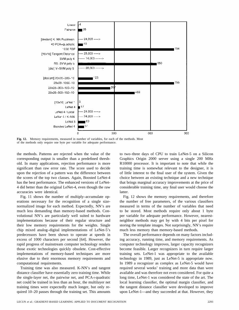
Fig. 12. Memory requirements, measured in number of variables, for each of the methods. Mostof the methods only require one byte per variable for adequate performance.

the methods. Patterns are rejected when the value of thecorresponding output is smaller than a predefined thresh-old. In many applications, rejection performance is moresignificant than raw error rate. The score used to decideupon the rejection of a pattern was the difference betweenthe scores of the top two classes. Again, Boosted LeNet-4has the best performance. The enhanced versions of LeNet-4 did better than the original LeNet-4, even though the rawaccuracies were identical.

Fig. 11 shows the number of multiply–accumulate op-erations necessary for the recognition of a single size-normalized image for each method. Expectedly, NN’s aremuch less demanding than memory-based methods. Con-volutional NN’s are particularly well suited to hardwareimplementations because of their regular structure andtheir low memory requirements for the weights. Singlechip mixed analog–digital implementations of LeNet-5’spredecessors have been shown to operate at speeds inexcess of 1000 characters per second [64]. However, therapid progress of mainstream computer technology rendersthose exotic technologies quickly obsolete. Cost-effectiveimplementations of memory-based techniques are moreelusive due to their enormous memory requirements andcomputational requirements.

Training time was also measured. K-NN’s and tangentdistance classifier have essentially zero training time. Whilethe single-layer net, the pairwise net, and PCAquadraticnet could be trained in less than an hour, the multilayer nettraining times were expectedly much longer, but only re-quired 10–20 passes through the training set. This amounts

to two–three days of CPU to train LeNet-5 on a SiliconGraphics Origin 2000 server using a single 200 MHzR10000 processor. It is important to note that while thetraining time is somewhat relevant to the designer, it isof little interest to the final user of the system. Given thechoice between an existing technique and a new techniquethat brings marginal accuracy improvements at the price ofconsiderable training time, any final user would choose thelatter.

Fig. 12 shows the memory requirements, and thereforethe number of free parameters, of the various classifiersmeasured in terms of the number of variables that needto be stored. Most methods require only about 1 byteper variable for adequate performance. However, nearest-neighbor methods may get by with 4 bits per pixel forstoring the template images. Not surprisingly, NN’s requiremuch less memory than memory-based methods.

The overall performance depends on many factors includ-ing accuracy, running time, and memory requirements. Ascomputer technology improves, larger capacity recognizersbecome feasible. Larger recognizers in turn require largertraining sets. LeNet-1 was appropriate to the availabletechnology in 1989, just as LeNet-5 is appropriate now.In 1989 a recognizer as complex as LeNet-5 would haverequired several weeks’ training and more data than wereavailable and was therefore not even considered. For quite along time, LeNet-1 was considered the state of the art. Thelocal learning classifier, the optimal margin classifier, andthe tangent distance classifier were developed to improveupon LeNet-1—and they succeeded at that. However, they


in turn motivated a search for improved NN architectures.This search was guided in part by estimates of the capacityof various learning machines, derived from measurementsof the training and test error as a function of the numberof training examples. We discovered that more capacitywas needed. Through a series of experiments in architec-ture, combined with an analysis of the characteristics ofrecognition errors, LeNet-4 and LeNet-5 were crafted.

We find that boosting gives a substantial improvement inaccuracy, with a relatively modest penalty in memory andcomputing expense. Also, distortion models can be usedto increase the effective size of a data set without actuallyrequiring to collect more data.

The SVM has excellent accuracy, which is most remark-able because, unlike the other high performance classifiers,it does not includea priori knowledge about the problem.In fact, this classifier would do just as well if the imagepixels were permuted with a fixed mapping and lost theirpictorial structure. However, reaching levels of performancecomparable to the convolutional NN’s can only be doneat considerable expense in memory and computational re-quirements. The RS-SVM requirements are within a factorof two of the convolutional networks, and the error rate isvery close. Improvements of those results are expected asthe technique is relatively new.

When plenty of data are available, many methods canattain respectable accuracy. The neural-net methods runmuch faster and require much less space than memory-based techniques. The NN’s advantage will become morestriking as training databases continue to increase in size.

E. Invariance and Noise Resistance

Convolutional networks are particularly well suited forrecognizing or rejecting shapes with widely varying size,position, and orientation, such as the ones typically pro-duced by heuristic segmenters in real-world string recog-nition systems.

In an experiment like the one described above, theimportance of noise resistance and distortion invariance isnot obvious. The situation in most real applications is quitedifferent. Characters generally must be segmented out oftheir context prior to recognition. Segmentation algorithmsare rarely perfect and often leave extraneous marks in char-acter images (noise, underlines, neighboring characters), orsometimes cut characters too much and produce incompletecharacters. Those images cannot be reliably size-normalizedand centered. Normalizing incomplete characters can bevery dangerous. For example, an enlarged stray mark canlook like a genuine “1.” Therefore, many systems haveresorted to normalizing the images at the level of fields orwords. In our case, the upper and lower profiles of entirefields (i.e., amounts in a check) are detected and used tonormalize the image to a fixed height. While this guaranteesthat stray marks will not be blown up into character-looking images, this also creates wide variations of thesize and vertical position of characters after segmentation.Therefore it is preferable to use a recognizer that is robustto such variations. Fig. 13 shows several examples of

distorted characters that are correctly recognized by LeNet-5. It is estimated that accurate recognition occurs forscale variations up to about a factor of two, vertical shiftvariations of plus or minus about half the height of thecharacter, and rotations up to plus or minus 30 degrees.While fully invariant recognition of complex shapes is stillan elusive goal, it seems that convolutional networks offera partial answer to the problem of invariance or robustnesswith respect to geometrical distortions.

Fig. 13 includes examples of the robustness of LeNet-5under extremely noisy conditions. Processing those imageswould pose insurmountable problems of segmentation andfeature extraction to many methods, but LeNet-5 seemsable to robustly extract salient features from these clutteredimages. The training set used for the network shown herewas the MNIST training set with salt and pepper noiseadded. Each pixel was randomly inverted with probability0.1.2

IV. M ULTIMODULE SYSTEMS AND GRAPH

TRANSFORMER NETWORKS

The classical back-propagation algorithm, as describedand used in the previous sections, is a simple form ofgradient-based learning. However, it is clear that the gra-dient back-propagation algorithm given by (4) describes amore general situation than simple multilayer feedforwardnetworks composed of alternated linear transformations andsigmoidal functions. In principle, derivatives can be back-propagated through any arrangement of functional modules,as long as we can compute the product of the Jacobians ofthose modules by any vector. Why would we want to trainsystems composed of multiple heterogeneous modules? Theanswer is that large and complex trainable systems need tobe built out of simple, specialized modules. The simplestexample is LeNet-5, which mixes convolutional layers,subsampling layers, fully connected layers, and RBF layers.Another less trivial example, described in Sections IV-Aand IV-B, is a system for recognizing words, that canbe trained to simultaneously segment and recognize wordswithout ever being given the correct segmentation.

Fig. 14 shows an example of a trainable multimodularsystem. A multimodule system is defined by the functionimplemented by each of the modules and by the graph ofinterconnection of the modules to each other. The graphimplicitly defines a partial order according to which themodules must be updated in the forward pass. For examplein Fig. 14, module 0 is first updated, then modules 1 and2 are updated (possibly in parallel), followed by module3. Modules may or may not have trainable parameters.Loss functions, which measure the performance of thesystem, are implemented as module 4. In the simplest case,the loss function module receives an external input thatcarries the desired output. In this framework, there is noqualitative difference between trainable parameters (W1,

2More examples of LeNet-5 in action are available WWW:http://www.research.att.com/˜yann/ocr.


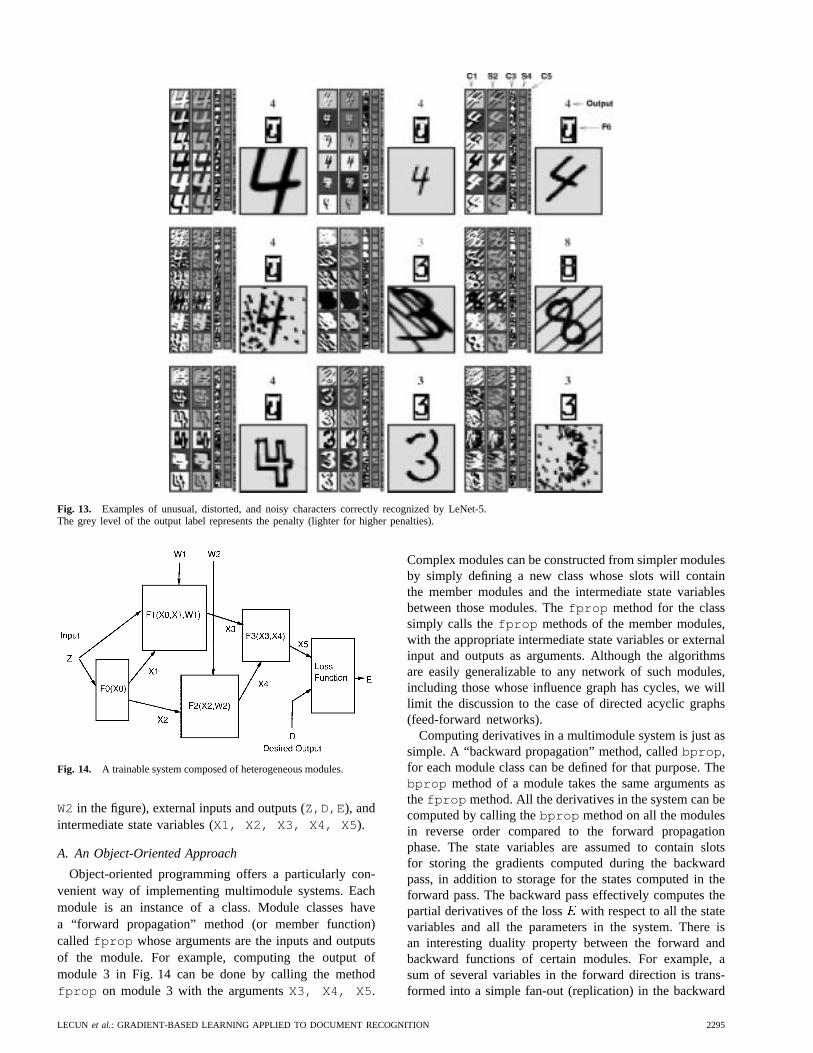
Fig. 13. Examples of unusual, distorted, and noisy characters correctly recognized by LeNet-5.The grey level of the output label represents the penalty (lighter for higher penalties).

Fig. 14. A trainable system composed of heterogeneous modules.

W2in the figure), external inputs and outputs (Z,D,E ), andintermediate state variables (X1, X2, X3, X4, X5 ).

A. An Object-Oriented Approach

Object-oriented programming offers a particularly con-venient way of implementing multimodule systems. Eachmodule is an instance of a class. Module classes havea “forward propagation” method (or member function)called fprop whose arguments are the inputs and outputsof the module. For example, computing the output ofmodule 3 in Fig. 14 can be done by calling the methodfprop on module 3 with the argumentsX3, X4, X5 .

Complex modules can be constructed from simpler modulesby simply defining a new class whose slots will containthe member modules and the intermediate state variablesbetween those modules. Thefprop method for the classsimply calls thefprop methods of the member modules,with the appropriate intermediate state variables or externalinput and outputs as arguments. Although the algorithmsare easily generalizable to any network of such modules,including those whose influence graph has cycles, we willlimit the discussion to the case of directed acyclic graphs(feed-forward networks).

Computing derivatives in a multimodule system is just assimple. A “backward propagation” method, calledbprop ,for each module class can be defined for that purpose. Thebprop method of a module takes the same arguments asthe fprop method. All the derivatives in the system can becomputed by calling thebprop method on all the modulesin reverse order compared to the forward propagationphase. The state variables are assumed to contain slotsfor storing the gradients computed during the backwardpass, in addition to storage for the states computed in theforward pass. The backward pass effectively computes thepartial derivatives of the loss with respect to all the statevariables and all the parameters in the system. There isan interesting duality property between the forward andbackward functions of certain modules. For example, asum of several variables in the forward direction is trans-formed into a simple fan-out (replication) in the backward


direction. Conversely, a fan-out in the forward directionis transformed into a sum in the backward direction. Thesoftware environment used to obtain the results describedin this paper, called SN3.1, uses the above concepts. Itis based on a home-grown object-oriented dialect of Lispwith a compiler to C.

The fact that derivatives can be computed by propagationin the reverse graph is easy to understand intuitively. Thebest way to justify it theoretically is through the use ofLagrange functions [21], [22]. The same formalism can beused to extend the procedures to networks with recurrentconnections.

B. Special Modules

NN’s and many other standard pattern recognition tech-niques can be formulated in terms of multimodular systemstrained with gradient-based learning. Commonly used mod-ules include matrix multiplications and sigmoidal modules,the combination of which can be used to build conven-tional NN’s. Other modules include convolutional layers,subsampling layers, RBF layers, and “softmax” layers [65].Loss functions are also represented as modules whosesingle output produces the value of the loss. Commonlyused modules have simplebprop methods. In general, thebprop method of a function is a multiplication by theJacobian of Here are a few commonly used examples.The bprop method of a fanout (a “Y” connection) is asum, and vice versa. Thebprop method of a multipli-cation by a coefficient is a multiplication by the samecoefficient. Thebprop method of a multiplication by amatrix is a multiplication by the transpose of that matrix.The bprop method of an addition with a constant is theidentity.

Interestingly, certain nondifferentiable modules can beinserted in a multimodule system without adverse effect.An interesting example of that is the multiplexer module.It has two (or more) regular inputs, one switching input, andone output. The module selects one of its inputs, dependingupon the (discrete) value of the switching input, and copiesit on its output. While this module is not differentiablewith respect to the switching input, it is differentiable withrespect to the regular inputs. Therefore the overall functionof a system that includes such modules will be differentiablewith respect to its parameters as long as the switching inputdoes not depend upon the parameters. For example, theswitching input can be an external input.

Another interesting case is themin module. This modulehas two (or more) inputs and one output. The output ofthe module is the minimum of the inputs. The functionof this module is differentiable everywhere, except onthe switching surface which is a set of measure zero.Interestingly, this function is continuous and reasonablyregular, and that is sufficient to ensure the convergenceof a gradient-based learning algorithm.

The object-oriented implementation of the multimoduleidea can easily be extended to include abbprop methodthat propagates Gauss–Newton approximations of the sec-ond derivatives. This leads to a direct generalization for

modular systems of the second-derivative back propagation(22) given in Appendix C.

The multiplexer module is a special case of a much moregeneral situation, described at length in Section IX, wherethe architecture of the system changes dynamically with theinput data. Multiplexer modules can be used to dynamicallyrewire (or reconfigure) the architecture of the system foreach new input pattern.

C. GTN’s

Multimodule systems are very flexible tools for build-ing a large trainable system. However, the descriptionsin the previous sections implicitly assumed that the setof parameters, and the state information communicatedbetween the modules, are all fixed-size vectors. The limitedflexibility of fixed-size vectors for data representation isa serious deficiency for many applications, notably fortasks that deal with variable length inputs (e.g., continuousspeech recognition and handwritten word recognition) or fortasks that require encoding relationships between objects orfeatures whose number and nature can vary (invariant per-ception, scene analysis, recognition of composite objects).An important special case is the recognition of strings ofcharacters or words.

More generally, fixed-size vectors lack flexibility fortasks in which the state must encode probability distribu-tions over sequences of vectors or symbols, as is the case inlinguistic processing. Such distributions over sequences arebest represented by stochastic grammars, or, in the moregeneral case, directed graphs in which each arc containsa vector (stochastic grammars are special cases in whichthe vector contains probabilities and symbolic information).Each path in the graph represents a different sequence ofvectors. Distributions over sequences can be representedby interpreting elements of the data associated with eacharc as parameters of a probability distribution or simplyas a penalty. Distributions over sequences are particularlyhandy for modeling linguistic knowledge in speech orhandwriting recognition systems: each sequence, i.e., eachpath in the graph, represents an alternative interpretationof the input. Successive processing modules progressivelyrefine the interpretation. For example, a speech recognitionsystem might start with a single sequence of acousticvectors, transform it into a lattice of phonemes (distributionover phoneme sequences), then into a lattice of words(distribution over word sequences), and then into a singlesequence of words representing the best interpretation.

In our work on building large-scale handwriting recog-nition systems, we have found that these systems could bedeveloped and designed much more easily and quickly byviewing the system as a networks of modules that take oneor several graphs as input and produce graphs as output.Such modules are called GT’s, and the complete systemsare called GTN’s. Modules in a GTN communicate theirstates and gradients in the form of directed graphs whosearcs carry numerical information (scalars or vectors) [66].

From the statistical point of view, the fixed-size state vec-tors of conventional networks can be seen as representing


(a) (b)

Fig. 15. Traditional NN’s and multimodule systems communi-cate fixed-size vectors between layers. Multilayer GTN’s arecomposed of trainable modules that operate on and produce graphswhose arcs carry numerical information.

the means of distributions in state space. In variable-sizenetworks such as the space-displacement NN’s describedin Section VII, the states are variable-length sequencesof fixed size vectors. They can be seen as representingthe mean of a probability distribution over variable-lengthsequences of fixed-size vectors. In GTN’s the states arerepresented as graphs, which can be seen as represent-ing mixtures of probability distributions over structuredcollections (possibly sequences) of vectors (Fig. 15).

One of the main points of the next several sections isto show that gradient-based learning procedures are notlimited to networks of simple modules that communicatethrough fixed-size vectors but can be generalized toGTN’s. Gradient back propagation through a GT takesgradients with respect to the numerical information inthe output graph and computes gradients with respect tothe numerical information attached to the input graphs,and with respect to the module’s internal parameters.Gradient-based learning can be applied as long asdifferentiable functions are used to produce the numericaldata in the output graph from the numerical data in theinput graph and the functions parameters.

The second point of the next several sections is to showthat the functions implemented by many of the modulesused in typical document processing systems (and otherimage recognition systems), though commonly thought tobe combinatorial in nature, are indeed differentiable withrespect to their internal parameters as well as with respectto their inputs, and are therefore usable as part of a globallytrainable system.

In most of the following, we will purposely avoid makingreferences to probability theory. All the quantities manipu-lated are viewed as penalties, or costs, which if necessarycan be transformed into probabilities by taking exponentialsand normalizing.

V. MULTIPLE OBJECT RECOGNITION: HOS

One of the most difficult problems of handwriting recog-nition is to recognize not just isolated characters, but

Fig. 16. Building a segmentation graph with HOS.

strings of characters such as zip codes, check amounts,or words. Since most recognizers can only deal with onecharacter at a time, we must first segment the stringinto individual character images. However, it is almostimpossible to devise image analysis techniques that willinfallibly segment naturally written sequences of charactersinto well formed characters.

The recent history of automatic speech recognition [28],[67] is here to remind us that training a recognizer byoptimizing a global criterion (at the word or sentence level)is much preferable to merely training it on hand-segmentedphonemes or other units. Several recent works have shownthat the same is true for handwriting recognition [38]:optimizing a word-level criterion is preferable to solelytraining a recognizer on presegmented characters becausethe recognizer can learn not only to recognize individualcharacters, but also to reject missegmented characters,thereby minimizing the overall word error.

This section and Section VI describe in detail a simpleexample of GTN to address the problem of reading stringsof characters, such as words or check amounts. The methodavoids the expensive and unreliable task of hand-truthingthe result of the segmentation often required in moretraditional systems trained on individually labeled characterimages.

A. Segmentation Graph

A now classical method for segmentation and recognitionis called HOS [68], [69]. Its main advantages over otherapproaches to segmentation are that it avoids making harddecisions about the segmentation by taking a large numberof different segmentations into consideration. The idea is touse heuristic image processing techniques to find candidatecuts of the word or string, and then to use the recognizer toscore the alternative segmentations thereby generated. Theprocess is depicted in Fig. 16. First, a number of candidatecuts are generated. Good candidate locations for cuts can befound by locating minima in the vertical projection profile,or minima of the distance between the upper and lowercontours of the word. Better segmentation heuristics aredescribed in Section XI. The cut generation heuristic isdesigned so as to generate more cuts than necessary in thehope that the “correct” set of cuts will be included. Once thecuts have been generated, alternative segmentations are bestrepresented by a graph, called the segmentation graph. Thesegmentation graph is a directed acyclic graph with a startnode and an end node. Each internal node is associated witha candidate cut produced by the segmentation algorithm.Each arc between a source node and a destination node


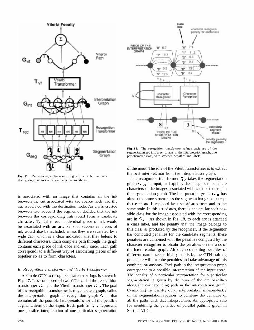
Fig. 17. Recognizing a character string with a GTN. For read-ability, only the arcs with low penalties are shown.

is associated with an image that contains all the inkbetween the cut associated with the source node and thecut associated with the destination node. An arc is createdbetween two nodes if the segmentor decided that the inkbetween the corresponding cuts could form a candidatecharacter. Typically, each individual piece of ink wouldbe associated with an arc. Pairs of successive pieces ofink would also be included, unless they are separated by awide gap, which is a clear indication that they belong todifferent characters. Each complete path through the graphcontains each piece of ink once and only once. Each pathcorresponds to a different way of associating pieces of inktogether so as to form characters.

B. Recognition Transformer and Viterbi Transformer

A simple GTN to recognize character strings is shown inFig. 17. It is composed of two GT’s called the recognitiontransformer and the Viterbi transformer The goalof the recognition transformer is to generate a graph, calledthe interpretation graph or recognition graph thatcontains all the possible interpretations for all the possiblesegmentations of the input. Each path in representsone possible interpretation of one particular segmentation

Fig. 18. The recognition transformer refines each arc of thesegmentation arc into a set of arcs in the interpretation graph, oneper character class, with attached penalties and labels.

of the input. The role of the Viterbi transformer is to extractthe best interpretation from the interpretation graph.

The recognition transformer takes the segmentationgraph as input, and applies the recognizer for singlecharacters to the images associated with each of the arcs inthe segmentation graph. The interpretation graph hasalmost the same structure as the segmentation graph, exceptthat each arc is replaced by a set of arcs from and to thesame node. In this set of arcs, there is one arc for each pos-sible class for the image associated with the correspondingarc in As shown in Fig. 18, to each arc is attacheda class label, and the penalty that the image belongs tothis class as produced by the recognizer. If the segmentorhas computed penalties for the candidate segments, thesepenalties are combined with the penalties computed by thecharacter recognizer to obtain the penalties on the arcs ofthe interpretation graph. Although combining penalties ofdifferent nature seems highly heuristic, the GTN trainingprocedure will tune the penalties and take advantage of thiscombination anyway. Each path in the interpretation graphcorresponds to a possible interpretation of the input word.The penalty of a particular interpretation for a particularsegmentation is given by the sum of the arc penaltiesalong the corresponding path in the interpretation graph.Computing the penalty of an interpretation independentlyof the segmentation requires to combine the penalties ofall the paths with that interpretation. An appropriate rulefor combining the penalties of parallel paths is given inSection VI-C.


The Viterbi transformer produces a graph with asingle path. This path is the path of least cumulated penaltyin the Interpretation graph. The result of the recognitioncan be produced by reading off the labels of the arcs alongthe graph extracted by the Viterbi transformer. TheViterbi transformer owes its name to the famous Viterbialgorithm [70], an application of the principle of dynamicprogramming to find the shortest path in a graph efficiently.Let be the penalty associated to arc with sourcenode and destination node (note that there can bemultiple arcs between two nodes). In the interpretationgraph, arcs also have a label The Viterbi algorithmproceeds as follows. Each node is associated with acumulated Viterbi penalty Those cumulated penaltiesare computed in any order that satisfies the partial orderdefined by the interpretation graph (which is directed andacyclic). The start node is initialized with the cumulatedpenalty The other nodes cumulated penalties

are computed recursively from the values of theirparent nodes, through the upstream arcs withdestination

(10)

Furthermore, the value of for each node which min-imizes the right-hand side is noted the minimizingentering arc. When the end node is reached we obtain in

the total penalty of the path with the smallest totalpenalty. We call this penalty the Viterbi penalty, and thissequence of arcs and nodes the Viterbi path. To obtain theViterbi path with nodes and arcs wetrace back these nodes and arcs as follows, starting with

the end node, and recursively using the minimizingentering arc: and until the start nodeis reached. The label sequence can then be read off the arcsof the Viterbi path.

VI. GLOBAL TRAINING FOR GRAPH

TRANSFORMER NETWORKS

Section V described the process of recognizing a stringusing HOS, assuming that the recognizer is trained soas to give low penalties for the correct class label ofcorrectly segmented characters, high penalties for erroneouscategories of correctly segmented characters, and highpenalties for all categories for poorly formed characters.This section explains how to train the system at the stringlevel to do the above without requiring manual labeling ofcharacter segments. This training will be performed witha GTN whose architecture is slightly different from therecognition architecture described in Section V.

In many applications, there is enougha priori knowledgeabout what is expected from each of the modules in orderto train them separately. For example, with HOS onecould individually label single-character images and traina character recognizer on them, but it might be difficultto obtain an appropriate set of noncharacter images totrain the model to reject wrongly segmented candidates.Although separate training is simple, it requires additional

supervision information that is often lacking or incomplete(the correct segmentation and the labels of incorrect candi-date segments). Furthermore, it can be shown that separatetraining is suboptimal [67].

The following section describes four different gradient-based methods for training GTN-based handwriting recog-nizers at the string level: Viterbi training, discriminativeViterbi training, forward training, and discriminative for-ward training. The last one is a generalization to graph-based systems of the maximuma posteriori criterion in-troduced in Section II-C. Discriminative forward trainingis somewhat similar to the so-called maximum mutualinformation criterion used to train HMM in speech recog-nition. However, our rationale differs from the classicalone. We make no recourse to a probabilistic interpretationbut show that, within the gradient-based learning approach,discriminative training is a simple instance of the pervasiveprinciple of error correcting learning.

Training methods for graph-based sequence recognitionsystems such as HMM’s have been extensively studiedin the context of speech recognition [28]. Those meth-ods require that the system be based on probabilisticgenerative models of the data, which provide normalizedlikelihoods over the space of possible input sequences.Popular HMM learning methods, such as the Baum–Welshalgorithm, rely on this normalization. The normalizationcannot be preserved when nongenerative models such asNN’s are integrated into the system. Other techniques, suchas discriminative training methods, must be used in thiscase. Several authors have proposed such methods to trainNN/HMM speech recognizers at the word or sentence level[29], [67], [71]–[78].

Other globally trainable sequence recognition systemsavoid the difficulties of statistical modeling by not resortingto graph-based techniques. The best example is recurrentNN’s (RNN’s). Unfortunately, despite early enthusiasm,the training of RNN’s with gradient-based techniques hasproven very difficult in practice [79].

The GTN techniques presented below simplify and gen-eralize the global training methods developed for speechrecognition.

A. Viterbi Training

During recognition, we select the path in the interpre-tation graph that has the lowest penalty with the Viterbialgorithm. Ideally, we would like this path of lowest penaltyto be associated with the correct label sequence as often aspossible. An obvious loss function to minimize is thereforethe average over the training set of the penalty of thepath associated with the correct label sequence that has thelowest penalty. The goal of training will be to find the set ofrecognizer parameters (the weights, if the recognizer is anNN) that minimize the average penalty of this “correct”lowest penalty path. The gradient of this loss functioncan be computed by back propagation through the GTNarchitecture shown in Fig. 19. This training architecture isalmost identical to the recognition architecture describedin the previous section, except that an extra GT called a


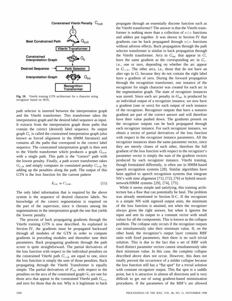
Fig. 19. Viterbi training GTN architecture for a character stringrecognizer based on HOS.

path selector is inserted between the interpretation graphand the Viterbi transformer. This transformer takes theinterpretation graph and the desired label sequence as input.It extracts from the interpretation graph those paths thatcontain the correct (desired) label sequence. Its outputgraph is called the constrained interpretation graph (alsoknown as forced alignment in the HMM literature) andcontains all the paths that correspond to the correct labelsequence. The constrained interpretation graph is then sentto the Viterbi transformer which produces a graphwith a single path. This path is the “correct” path withthe lowest penalty. Finally, a path scorer transformer takes

and simply computes its cumulated penalty byadding up the penalties along the path. The output of thisGTN is the loss function for the current pattern

(11)

The only label information that is required by the abovesystem is the sequence of desired character labels. Noknowledge of the correct segmentation is required onthe part of the supervisor, since it chooses among thesegmentations in the interpretation graph the one that yieldsthe lowest penalty.

The process of back propagating gradients through theViterbi training GTN is now described. As explained inSection IV, the gradients must be propagated backwardthrough all modules of the GTN in order to computegradients in preceding modules and thereafter tune theirparameters. Back propagating gradients through the pathscorer is quite straightforward. The partial derivatives ofthe loss function with respect to the individual penalties onthe constrained Viterbi path are equal to one, sincethe loss function is simply the sum of those penalties. Backpropagating through the Viterbi Transformer is equallysimple. The partial derivatives of with respect to thepenalties on the arcs of the constrained graphare one forthose arcs that appear in the constrained Viterbi pathand zero for those that do not. Why is it legitimate to back

propagate through an essentially discrete function such asthe Viterbi transformer? The answer is that the Viterbi trans-former is nothing more than a collection ofmin functionsand adders put together. It was shown in Section IV thatgradients can be back propagated throughmin functionswithout adverse effects. Back propagation through the pathselector transformer is similar to back propagation throughthe Viterbi transformer. Arcs in that appear inhave the same gradient as the corresponding arc ini.e., one or zero, depending on whether the arc appearin The other arcs, i.e., those that do not have analter ego in because they do not contain the right labelhave a gradient of zero. During the forward propagationthrough the recognition transformer, one instance of therecognizer for single character was created for each arc inthe segmentation graph. The state of recognizer instanceswas stored. Since each arc penalty in is produced byan individual output of a recognizer instance, we now havea gradient (one or zero) for each output of each instanceof the recognizer. Recognizer outputs that have a nonzerogradient are part of the correct answer and will thereforehave their value pushed down. The gradients present onthe recognizer outputs can be back propagated througheach recognizer instance. For each recognizer instance, weobtain a vector of partial derivatives of the loss functionwith respect to the recognizer instance parameters. All therecognizer instances share the same parameter vector, sincethey are merely clones of each other, therefore the fullgradient of the loss function with respect to the recognizer’sparameter vector is simply the sum of the gradient vectorsproduced by each recognizer instance. Viterbi training,though formulated differently, is often use in HMM-basedspeech recognition systems [28]. Similar algorithms havebeen applied to speech recognition systems that integrateNN’s with time alignment [71], [72], [76] or hybrid neural-network/HMM systems [29], [74], [75].

While it seems simple and satisfying, this training archi-tecture has a flaw that can potentially be fatal. The problemwas already mentioned in Section II-C. If the recognizeris a simple NN with sigmoid output units, the minimumof the loss function is attained, not when the recognizeralways gives the right answer, but when it ignores theinput and sets its output to a constant vector with smallvalues for all the components. This is known as the collapseproblem. The collapse only occurs if the recognizer outputscan simultaneously take their minimum value. If, on theother hand, the recognizer’s output layer contains RBFunits with fixed parameters, then there is no such trivialsolution. This is due to the fact that a set of RBF withfixed distinct parameter vectors cannot simultaneously taketheir minimum value. In this case, the complete collapsedescribed above does not occur. However, this does nottotally prevent the occurrence of a milder collapse becausethe loss function still has a “flat spot” for a trivial solutionwith constant recognizer output. This flat spot is a saddlepoint, but it is attractive in almost all directions and is verydifficult to get out of using gradient-based minimizationprocedures. If the parameters of the RBF’s are allowed


to adapt, then the collapse problems reappear because theRBF centers can all converge to a single vector, and theunderlying NN can learn to produce that vector and ignorethe input. A different kind of collapse occurs if the widthof the RBF’s are also allowed to adapt. The collapse onlyoccurs if a trainable module such as an NN feeds theRBF’s. The collapse does not occur in HMM-based speechrecognition systems because they are generative systemsthat produce normalized likelihoods for the input data (moreon this later). Another way to avoid the collapse is to trainthe whole system with respect to a discriminative trainingcriterion, such as maximizing the conditional probability ofthe correct interpretations (correct sequence of class labels)given the input image.

Another problem with Viterbi training is that the penaltyof the answer cannot be used reliably as a measure ofconfidence because it does not take low-penalty (or high-scoring) competing answers into account.

B. Discriminative Viterbi Training

A modification of the training criterion can circumventthe collapse problem described above and at the same timeproduce more reliable confidence values. The idea is tonot only minimize the cumulated penalty of the lowestpenalty path with the correct interpretation, but also tosomehow increase the penalty of competing and possiblyincorrect paths that have a dangerously low penalty. Thistype of criterion is called discriminative because it plays thegood answers against the bad ones. Discriminative trainingprocedures can be seen as attempting to build appropriateseparating surfaces between classes rather than to model in-dividual classes independently of each other. For example,modeling the conditional distribution of the classes giventhe input image is more discriminative (focusing more onthe classification surface) than having a separate generativemodel of the input data associated to each class (which, withclass priors, yields the whole joint distribution of classesand inputs). This is because the conditional approach doesnot need to assume a particular form for the distribution ofthe input data.

One example of discriminative criterion is the differencebetween the penalty of the Viterbi path in the constrainedgraph, and the penalty of the Viterbi path in the (uncon-strained) interpretation graph, i.e., the difference betweenthe penalty of the best correct path and the penalty ofthe best path (correct or incorrect). The correspondingGTN training architecture is shown in Fig. 20. The leftside of the diagram is identical to the GTN used fornondiscriminative Viterbi training. This loss function re-duces the risk of collapse because it forces the recognizerto increases the penalty of wrongly recognized objects.Discriminative training can also be seen as another exampleof error correction procedure, which tends to minimize thedifference between the desired output computed in the lefthalf of the GTN in Fig. 20 and the actual output computedin the right half of Fig. 20.

Let the discriminative Viterbi loss function be denotedand let us call the penalty of the Viterbi path

in the constrained graph and the penalty of the Viterbipath in the unconstrained interpretation graph

(12)

is always positive since the constrained graph is asubset of the paths in the interpretation graph, and theViterbi algorithm selects the path with the lowest totalpenalty. In the ideal case, the two paths andcoincide, and is zero.

Back-propagating gradients through the discriminativeViterbi GTN adds some “negative” training to the previ-ously described nondiscriminative training. Fig. 20 showshow the gradients are back propagated. The left half isidentical to the nondiscriminative Viterbi training GTN,therefore the back propagation is identical. The gradientsback propagated through the right half of the GTN aremultiplied by 1, since contributes to the loss witha negative sign. Otherwise the process is similar to the lefthalf. The gradients on arcs of get positive contributionsfrom the left half and negative contributions from theright half. The two contributions must be added since thepenalties on arcs are sent to the two halves througha “Y” connection in the forward pass. Arcs in thatappear neither in nor in have a gradient of zero.They do not contribute to the cost. Arcs that appear in both

and also have zero gradient. The1 contributionfrom the right half cancels the1 contribution from the lefthalf. In other words, when an arc is rightfully part of theanswer there is no gradient. If an arc appears in butnot in the gradient is 1. The arc should have had alower penalty to make it to If an arc is in butnot in the gradient is The arc had a low penalty,but it should have had a higher penalty since it is not partof the desired answer.

Variations of this technique have been used for the speechrecognition. Driancourt and Bottou [76] used a version ofit where the loss function is saturated to a fixed value.This can be seen as a generalization of the Learning VectorQuantization 2 (LVQ-2) loss function [80]. Other variationsof this method use not only the Viterbi path but the K-best paths. The discriminative Viterbi algorithm does nothave the flaws of the nondiscriminative version, but thereare problems nonetheless. The main problem is that thecriterion does not build a margin between the classes. Thegradient is zero as soon as the penalty of the constrainedViterbi path is equal to that of the Viterbi path. It would bedesirable to push up the penalties of the wrong paths whenthey are dangerously close to the good one. The followingsection presents a solution to this problem.

C. Forward Scoring and Forward Training

While the penalty of the Viterbi path is perfectly appro-priate for the purpose of recognition it gives only a partialpicture of the situation. Imagine the lowest penalty pathscorresponding to several different segmentations producedthe same answer (the same label sequence). Then it could beargued that the overall penalty for the interpretation should


Fig. 20. Discriminative Viterbi training GTN architecture for a character string recognizer basedon HOS. Quantities in square brackets are penalties computed during the forward propagation.Quantities in parentheses are partial derivatives computed during the backward propagation.

be smaller than the penalty obtained when only one pathproduced that interpretation, because multiple paths withidentical label sequences are more evidence that the labelsequence is correct. Several rules can be used computethe penalty associated to a graph that contains severalparallel paths. We use a combination rule borrowed froma probabilistic interpretation of the penalties as negativelog posteriors. In a probabilistic framework, the posteriorprobability for the interpretation should be the sum of theposteriors for all the paths that produce that interpretation.

Translated in terms of penalties, the penalty of an inter-pretation should be the negative logarithm of the sum ofthe negative exponentials of the penalties of the individualpaths. The overall penalty will be smaller than all thepenalties of the individual paths.

Given an interpretation, there is a well-known method,called the forward algorithm for computing the abovequantity efficiently [28]. The penalty computed with thisprocedure for a particular interpretation is called the for-ward penalty. Consider again the concept of constrained


graph, the subgraph of the interpretation graph whichcontains only the paths that are consistent with a particularlabel sequence. There is one constrained graph for eachpossible label sequence (some may be empty graphs, whichhave infinite penalties). Given an interpretation, runningthe forward algorithm on the corresponding constrainedgraph gives the forward penalty for that interpretation.The forward algorithm proceeds in a way very similar tothe Viterbi algorithm, except that the operation used ateach node to combine the incoming cumulated penalties,instead of being themin function, is the so-calledlogaddoperation, which can be seen as a “soft” version of theminfunction

(13)

where is the set of upstream arcs of nodeis the penalty on arc and

(14)

Note that because of numerical inaccuracies, it is betterto factorize the largest (corresponding to the smallestpenalty) out of the logarithm.

An interesting analogy can be drawn if we considerthat a graph on which we apply the forward algorithm isequivalent to an NN on which we run a forward propaga-tion, except that multiplications are replaced by additions,the additions are replaced by log-adds, and there are nosigmoids.

One way to understand the forward algorithm is to thinkabout multiplicative scores (e.g., probabilities) instead ofadditive penalties on the arcs: scoreIn that case the Viterbi algorithm selects the path withthe largest cumulative score (with scores multiplied alongthe path), whereas the forward score is the sum of thecumulative scores associated to each of the possible pathsfrom the start to the end node. The forward penalty isalways lower than the cumulated penalty on any of thepaths, but if one path “dominates” (with a much lowerpenalty), its penalty is almost equal to the forward penalty.The forward algorithm gets its name from the forwardpass of the well-known Baum–Welsh algorithm for trainingHMM’s [28]. Section VIII-E gives more details on therelation between this work and HMM’s.

The advantage of the forward penalty with respect to theViterbi penalty is that it takes into account all the differentways to produce an answer, not just the one with the lowestpenalty. This is important if there is some ambiguity in thesegmentation, since the combined forward penalty of twopaths and associated with the same label sequencemay be less than the penalty of a path associated withanother label sequence, even though the penalty ofmight be less than any one of or

The forward-training GTN is only a slight modification ofthe previously introduced Viterbi-training GTN. It sufficesto turn the Viterbi transformers in Fig. 19 into forwardscorers that take an interpretation graph as input an produce

the forward penalty of that graph on output. Then thepenalties of all the paths that contain the correct answerare lowered, instead of just that of the best one.

Back propagating through the forward penalty computa-tion (the forward transformer) is quite different from backpropagating through a Viterbi transformer. All the penaltiesof the input graph have an influence on the forward penalty,but penalties that belong to low-penalty paths have astronger influence. Computing derivatives with respect tothe forward penalties computed at each node of agraph is done by back-propagation through the graph

(15)

where with source is the set ofdownstream arcs from node From the above derivatives,the derivatives with respect to the arc penalties are obtained

(16)

This can be seen as a “soft” version of the back propagationthrough a Viterbi scorer and transformer. All the arcs in

have an influence on the loss function. The arcs thatbelong to low penalty paths have a larger influence. Backpropagation through the path selector is the same as before.The derivative with respect to arcs that have an alterego in are simply copied from the corresponding arc in

The derivatives with respect to the other arcs are zero.Several authors have applied the idea of back-propagating

gradients through a forward scorer to train speech recogni-tion systems, including Bridle and his-net model [73] andHaffner and his -TDNN model [81], but these authorsrecommended discriminative training as described in thenext section.

D. Discriminative Forward Training

The information contained in the forward penalty can beused in another discriminative training criterion which wewill call the discriminative forward criterion. This criterioncorresponds to maximization of the posterior probability ofchoosing the paths associated with the correct interpreta-tion. This posterior probability is defined as the exponentialof minus the constrained forward penalty, normalized by theexponential of minus the unconstrained forward penalty.Note that the forward penalty of the constrained graphis always larger or equal to the forward penalty of theunconstrained interpretation graph. Ideally, we would likethe forward penalty of the constrained graph to be equalto the forward penalty of the complete interpretation graph.Equality between those two quantities is achieved whenthe combined penalties of the paths with the correct labelsequence is negligibly small compared to the penalties of allthe other paths, or that the posterior probability associatedto the paths with the correct interpretation is almost one,which is precisely what we want. The corresponding GTNtraining architecture is shown in Fig. 21.

Let the difference be denoted and let us callthe forward penalty of the constrained graph and


Fig. 21. Discriminative forward training GTN architecture for acharacter string recognizer based on HOS.

the forward penalty of the complete interpretationgraph

(17)

is always positive since the constrained graph isa subset of the paths in the interpretation graph, and theforward penalty of a graph is always larger than the forwardpenalty of a subgraph of this graph. In the ideal case, thepenalties of incorrect paths are infinitely large, thereforethe two penalties coincide and is zero. Readersfamiliar with the Boltzmann machine connectionist modelmight recognize the constrained and unconstrained graphsas analogous to the “clamped” (constrained by the observedvalues of the output variable) and “free” (unconstrained)phases of the Boltzmann machine algorithm [13].

Back propagating derivatives through the discriminativeforward GTN distributes gradients more evenly than in theViterbi case. Derivatives are back propagated through theleft half of the GTN in Fig. 21 down to the interpretationgraph. Derivatives are negated and back propagated throughthe right-half, and the result for each arc is added to thecontribution from the left half. Each arc in now hasa derivative. Arcs that are part of a correct path havea positive derivative. This derivative is very large if anincorrect path has a lower penalty than all the correctpaths. Similarly, the derivatives with respect to arcs that arepart of a low-penalty incorrect path have a large negativederivative. On the other hand, if the penalty of a pathassociated with the correct interpretation is much smallerthan all other paths, the loss function is very close to zeroand almost no gradient is back propagated. The trainingtherefore concentrates on examples of images which yielda classification error, and furthermore, it concentrates on thepieces of the image which cause that error. Discriminativeforward training is an elegant and efficient way of solvingthe infamous credit assignment problem for learning ma-chines that manipulate “dynamic” data structures such asgraphs. More generally, the same idea can be used in all

situations where a learning machine must choose betweendiscrete alternative interpretations.

As previously, the derivatives on the interpretation graphpenalties can then be back propagated into the characterrecognizer instances. Back propagation through the charac-ter recognizer gives derivatives on its parameters. All thegradient contributions for the different candidate segmentsare added up to obtain the total gradient associated toone pair (input image, correct label sequence), that is, oneexample in the training set. A step of stochastic gradientdescent can then be applied to update the parameters.

E. Remarks on Discriminative Training

In the above discussion, the global training criterionwas given a probabilistic interpretation, but the individualpenalties on the arcs of the graphs were not. There aregood reasons for that. For example, if some penalties areassociated to the different class labels, they would: 1) haveto sum to one (class posteriors) or 2) integrate to one overthe input domain (likelihoods).

Let us first discuss the first case (class posteriors nor-malization). This local normalization of penalties mayeliminate information that is important for locally rejectingall the classes [82], e.g., when a piece of image doesnot correspond to a valid character class because some ofthe segmentation candidates may be wrong. Although anexplicit “garbage class” can be introduced in a probabilisticframework to address that question, some problems remainbecause it is difficult to characterize such a class probabilis-tically and to train a system in this way (it would requirea density model of unseen or unlabeled samples).

The probabilistic interpretation of individual variablesplays an important role in the Baum–Welsh algorithmin combination with the expectation-maximization (EM)procedure. Unfortunately, those methods cannot be appliedto discriminative training criteria, and one is reduced tousing gradient-based methods. Enforcing the normalizationof the probabilistic quantities while performing gradient-based learning is complex, inefficient, time consuming, andcreates ill-conditioning of the loss-function.

Following [82], we therefore prefer to postpone normal-ization as far as possible (in fact, until the final decisionstage of the system). Without normalization, the quantitiesmanipulated in the system do not have a direct probabilisticinterpretation.

Let us now discuss the second case (using a generativemodel of the input). Generative models build the boundaryindirectly by first building an independent density modelfor each class and then performing classification decisionson the basis of these models. This is not a discriminativeapproach in that it does not focus on the ultimate goal oflearning, which in this case is to learn the classificationdecision surface. Theoretical arguments [6], [7] suggest thatestimating input densities when the real goal is to obtaina discriminant function for classification is a suboptimalstrategy. In theory, the problem of estimating densitiesin high-dimensional spaces is much more ill posed thanfinding decision boundaries.


Fig. 22. Explicit segmentation can be avoided by sweeping arecognizer at every possible location in the input field.

Even though the internal variables of the system do nothave a direct probabilistic interpretation, the overall systemcan still be viewed as producing posterior probabilitiesfor the classes. In fact, assuming that a particular labelsequence is given as the “desired sequence” to the GTN inFig. 21, the exponential of minus can be interpretedas an estimate of the posterior probability of that labelsequence given the input. The sum of those posteriors forall the possible label sequences is one. Another approachwould consists of directly minimizing an approximationof the number of misclassifications [83], [76]. We preferto use the discriminative forward loss function because itcauses less numerical problems during the optimization. Wewill see in Section X-C that this is a good way to obtainscores on which to base a rejection strategy. The importantpoint being made here is that one is free to choose anyparameterization deemed appropriate for a classificationmodel. The fact that a particular parameterization usesinternal variables with no clear probabilistic interpretationdoes not make the model any less legitimate than modelsthat manipulate normalized quantities.

An important advantage of global and discriminativetraining is that learning focuses on the most importanterrors, and the system learns to integrate the ambiguitiesfrom the segmentation algorithm with the ambiguities ofthe character recognizer. In Section IX we present ex-perimental results with an online handwriting recognitionsystem that confirm the advantages of using global trainingversus separate training. Experiments in speech recognitionwith hybrids of NN’s and HMM’s also showed markedimprovements brought by global training [29], [67], [77],[84].

VII. M ULTIPLE OBJECT RECOGNITION: SPACE

DISPLACEMENT NEURAL NETWORK

There is a simple alternative to explicitly segmentingimages of character strings using heuristics. The idea isto sweep a recognizer at all possible locations across anormalized image of the entire word or string as shownin Fig. 22. With this technique, no segmentation heuristicsare required since the system essentially examines all thepossible segmentations of the input. However, there areproblems with this approach. First, the method is in general

Fig. 23. An SDNN is a convolutional network that has beenreplicated over a wide input field.

quite expensive. The recognizer must be applied at everypossible location on the input, or at least at a large enoughsubset of locations so that misalignments of charactersin the field of view of the recognizers are small enoughto have no effect on the error rate. Second, when therecognizer is centered on a character to be recognized,the neighbors of the center character will be present in thefield of view of the recognizer, possibly touching the centercharacter. Therefore the recognizer must be able to correctlyrecognize the character in the center of its input field, evenif neighboring characters are very close to or touching thecentral character. Third, a word or character string cannotbe perfectly size-normalized. Individual characters within astring may have widely varying sizes and baseline positions.Therefore the recognizer must be very robust to shifts andsize variations.

These three problems are elegantly circumvented if aconvolutional network is replicated over the input field.First of all, as shown in Section III, convolutional NN’s arevery robust to shifts and scale variations of the input image,as well as to noise and extraneous marks in the input. Theseproperties take care of the latter two problems mentionedin the previous paragraph. Second, convolutional networksprovide a drastic saving in computational requirement whenreplicated over large input fields. A replicated convolutionalnetwork, also called an SDNN [27], is shown in Fig. 23.While scanning a recognizer can be prohibitively expen-sive in general, convolutional networks can be scanned orreplicated very efficiently over large, variable-size inputfields. Consider one instance of a convolutional net and its


alter ego at a nearby location. Because of the convolutionalnature of the network, units in the two instances that lookat identical locations on the input have identical outputs,therefore their states do not need to be computed twice.Only a thin “slice” of new states that are not shared bythe two network instances needs to be recomputed. Whenall the slices are put together, the result is simply a largerconvolutional network whose structure is identical to theoriginal network, except that the feature maps are largerin the horizontal dimension. In other words, replicating aconvolutional network can be done simply by increasing thesize of the fields over which the convolutions are performedand by replicating the output layer accordingly. The outputlayer effectively becomes a convolutional layer. An outputwhose receptive field is centered on an elementary objectwill produce the class of this object, while an in-betweenoutput may indicate no character or contain rubbish. Theoutputs can be interpreted as evidences for the presence ofobjects at all possible positions in the input field.

The SDNN architecture seems particularly attractive forrecognizing cursive handwriting where no reliable segmen-tation heuristic exists. Although the idea of SDNN is quiteold and very attractive in its simplicity, it has not generatedwide interest until recently because, as stated above, it putsenormous demands on the recognizer [26], [27]. In speechrecognition, where the recognizer is at least one order ofmagnitude smaller, replicated convolutional networks areeasier to implement, for instance in Haffner’s multistateTDNN model [78], [85].

A. Interpreting the Output of an SDNN with a GTN

The output of an SDNN is a sequence of vectors whichencode the likelihoods, penalties, or scores of finding char-acter of a particular class label at the corresponding locationin the input. A postprocessor is required to pull out thebest possible label sequence from this vector sequence. Anexample of SDNN output is shown in Fig. 25. Very often,individual characters are spotted by several neighboringinstances of the recognizer, a consequence of the robustnessof the recognizer to horizontal translations. Also quiteoften, characters are erroneously detected by recognizerinstances that see only a piece of a character. For examplea recognizer instance that only sees the right third of a“4” might output the label 1. How can we eliminate thoseextraneous characters from the output sequence and pullout the best interpretation? This can be done using a newtype of GT with two input graphs as shown in Fig. 24.The sequence of vectors produced by the SDNN is firstcoded into a linear graph with multiple arcs between pairsof successive nodes. Each arc between a particular pair ofnodes contains the label of one of the possible categories,together with the penalty produced by the SDNN for thatclass label at that location. This graph is called the SDNNoutput graph. The second input graph to the transformeris a grammar transducer, more specifically a finite-statetransducer [86], that encodes the relationship between inputstrings of class labels and corresponding output stringsof recognized characters. The transducer is a weighted

Fig. 24. A GT pulls out the best interpretation from the outputof the SDNN.

Fig. 25. An example of multiple character recognition withSDNN. With SDNN, no explicit segmentation is performed.

finite state machine (a graph) where each arc contains apair of labels and possibly a penalty. Like a finite-statemachine, a transducer is in a state and follows an arcto a new state when an observed input symbol matchesthe first symbol in the symbol pair attached to the arc.At this point the transducer emits the second symbol inthe pair together with a penalty that combines the penaltyof the input symbol and the penalty of the arc. A trans-ducer therefore transforms a weighted symbol sequenceinto another weighted symbol sequence. The GT shownin Fig. 24 performs a composition between the recognitiongraph and the grammar transducer. This operation takesevery possible sequence corresponding to every possiblepath in the recognition graph and matches them with thepaths in the grammar transducer. The composition producesthe interpretation graph, which contains a path for eachcorresponding output label sequence. This compositionoperation may seem combinatorially intractable, but it turnsout there exists an efficient algorithm for it described inmore details in Section VIII.

B. Experiments with SDNN

In a series of experiments, LeNet-5 was trained with thegoal of being replicated so as to recognize multiple charac-ters without segmentations. The data were generated from


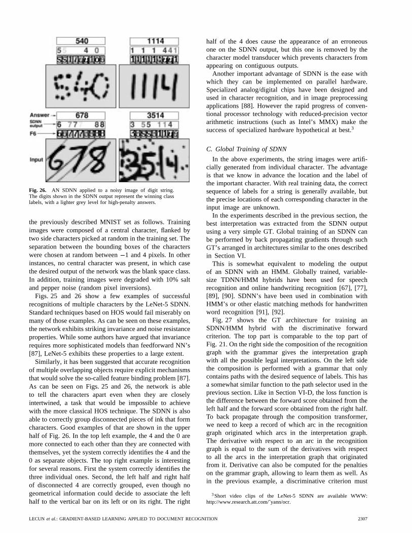
Fig. 26. AN SDNN applied to a noisy image of digit string.The digits shown in the SDNN output represent the winning classlabels, with a lighter grey level for high-penalty answers.

the previously described MNIST set as follows. Trainingimages were composed of a central character, flanked bytwo side characters picked at random in the training set. Theseparation between the bounding boxes of the characterswere chosen at random between1 and 4 pixels. In otherinstances, no central character was present, in which casethe desired output of the network was the blank space class.In addition, training images were degraded with 10% saltand pepper noise (random pixel inversions).

Figs. 25 and 26 show a few examples of successfulrecognitions of multiple characters by the LeNet-5 SDNN.Standard techniques based on HOS would fail miserably onmany of those examples. As can be seen on these examples,the network exhibits striking invariance and noise resistanceproperties. While some authors have argued that invariancerequires more sophisticated models than feedforward NN’s[87], LeNet-5 exhibits these properties to a large extent.

Similarly, it has been suggested that accurate recognitionof multiple overlapping objects require explicit mechanismsthat would solve the so-called feature binding problem [87].As can be seen on Figs. 25 and 26, the network is ableto tell the characters apart even when they are closelyintertwined, a task that would be impossible to achievewith the more classical HOS technique. The SDNN is alsoable to correctly group disconnected pieces of ink that formcharacters. Good examples of that are shown in the upperhalf of Fig. 26. In the top left example, the 4 and the 0 aremore connected to each other than they are connected withthemselves, yet the system correctly identifies the 4 and the0 as separate objects. The top right example is interestingfor several reasons. First the system correctly identifies thethree individual ones. Second, the left half and right halfof disconnected 4 are correctly grouped, even though nogeometrical information could decide to associate the lefthalf to the vertical bar on its left or on its right. The right

half of the 4 does cause the appearance of an erroneousone on the SDNN output, but this one is removed by thecharacter model transducer which prevents characters fromappearing on contiguous outputs.

Another important advantage of SDNN is the ease withwhich they can be implemented on parallel hardware.Specialized analog/digital chips have been designed andused in character recognition, and in image preprocessingapplications [88]. However the rapid progress of conven-tional processor technology with reduced-precision vectorarithmetic instructions (such as Intel’s MMX) make thesuccess of specialized hardware hypothetical at best.3

C. Global Training of SDNN

In the above experiments, the string images were artifi-cially generated from individual character. The advantageis that we know in advance the location and the label ofthe important character. With real training data, the correctsequence of labels for a string is generally available, butthe precise locations of each corresponding character in theinput image are unknown.

In the experiments described in the previous section, thebest interpretation was extracted from the SDNN outputusing a very simple GT. Global training of an SDNN canbe performed by back propagating gradients through suchGT’s arranged in architectures similar to the ones describedin Section VI.

This is somewhat equivalent to modeling the outputof an SDNN with an HMM. Globally trained, variable-size TDNN/HMM hybrids have been used for speechrecognition and online handwriting recognition [67], [77],[89], [90]. SDNN’s have been used in combination withHMM’s or other elastic matching methods for handwrittenword recognition [91], [92].

Fig. 27 shows the GT architecture for training anSDNN/HMM hybrid with the discriminative forwardcriterion. The top part is comparable to the top part ofFig. 21. On the right side the composition of the recognitiongraph with the grammar gives the interpretation graphwith all the possible legal interpretations. On the left sidethe composition is performed with a grammar that onlycontains paths with the desired sequence of labels. This hasa somewhat similar function to the path selector used in theprevious section. Like in Section VI-D, the loss function isthe difference between the forward score obtained from theleft half and the forward score obtained from the right half.To back propagate through the composition transformer,we need to keep a record of which arc in the recognitiongraph originated which arcs in the interpretation graph.The derivative with respect to an arc in the recognitiongraph is equal to the sum of the derivatives with respectto all the arcs in the interpretation graph that originatedfrom it. Derivative can also be computed for the penaltieson the grammar graph, allowing to learn them as well. Asin the previous example, a discriminative criterion must

3Short video clips of the LeNet-5 SDNN are available WWW:http://www.research.att.com/˜yann/ocr.


Fig. 27. A globally trainable SDNN/HMM hybrid system ex-pressed as a GTN.

be used, because using a nondiscriminative criterion couldresult in a collapse effect if the network’s output RBF areadaptive. The above training procedure can be equivalentlyformulated in term of HMM. Early experiments in zipcode recognition [91], and more recent experiments inonline handwriting recognition [38] have demonstrated theidea of globally trained SDNN/HMM hybrids. SDNN isan extremely promising and attractive technique for OCR,but so far it has not yielded better results than HOS. Wehope that these results will improve as more experience isgained with these models.

D. Object Detection and Spotting with SDNN

An interesting application of SDNN’s is object detectionand spotting. The invariance properties of convolutionalnetworks, combined with the efficiency with which theycan be replicated over large fields, suggests that they can beused for “brute force” object spotting and detection in largeimages. The main idea is to train a single convolutionalnetwork to distinguish images of the object of interest fromimages present in the background. In utilization mode, thenetwork is replicated so as to cover the entire image tobe analyzed, thereby forming a 2-D SDNN. The output ofthe SDNN is a 2-D plane in which activated units indicatethe presence of the object of interest in the correspondingreceptive field. Since the sizes of the objects to be detectedwithin the image are unknown, the image can be presentedto the network at multiple resolutions, and the results atmultiple resolutions combined. The idea has been appliedto face location [93], address block location on envelopes[94], and hand tracking in video [95].

To illustrate the method, we will consider the caseof face detection in images as described in [93]. First,

images containing faces at various scales are collected.Those images are filtered through a zero-mean Laplacianfilter so as to remove variations in global illumination andlow spatial frequency illumination gradients. Then, trainingsamples of faces and nonfaces are manually extracted fromthose images. The face subimages are then size normalizedso that the height of the entire face is approximately 20pixels while keeping fairly large variations (within a factorof two). The scale of background subimages are pickedat random. A single convolutional network is trained onthose samples to classify face subimages from nonfacesubimages.

When a scene image is to be analyzed, it is first filteredthrough the Laplacian filter and subsampled at powers-of-two resolutions. The network is replicated over each ofmultiple resolution images. A simple voting technique isused to combine the results from multiple resolutions.

A 2-D version of the global training method describedin the previous section can be used to alleviate the needto manually locate faces when building the training sample[93]. Each possible location is seen as an alternative inter-pretation, i.e., one of several parallel arcs in a simple graphthat only contains a start node and an end node.

Other authors have used NN’s or other classifiers suchas SVM’s for face detection with great success [96], [97].Their systems are very similar to the one described above,including the idea of presenting the image to the networkat multiple scales. But since those systems do not useconvolutional networks, they cannot take advantage of thespeedup described here, and they have to rely on othertechniques, such as prefiltering and real-time tracking,to keep the computational requirement within reasonablelimits. In addition, because those classifiers are much lessinvariant to scale variations than convolutional networks, itis necessary to multiply the number of scales at which theimages are presented to the classifier.

VIII. G RAPH TRANSFORMER NETWORKS

AND TRANSDUCERS

In Section IV, GTN’s were introduced as a general-ization of multilayer, multimodule networks where thestate information is represented as graphs instead of fixed-size vectors. This section reinterprets the GTN’s in theframework of generalized transduction and proposes apowerful graph composition algorithm.

A. Previous Work

Numerous authors in speech recognition have usedgradient-based learning methods that integrate graph-based statistical models (notably HMM’s) with acousticrecognition modules, mainly Gaussian mixture models,but also NN’s [67], [78], [98], [99]. Similar ideas havebeen applied to handwriting recognition (see [38] fora review). However, there has been no proposal for asystematic approach to multilayer graph-based trainablesystems. The idea of transforming graphs into other graphshas received considerable attention in computer science


through the concept of weighted finite-state transducers[86]. Transducers have been applied to speech recognition[100] and language translation [101], and proposals havebeen made for handwriting recognition [102]. This lineof work has been mainly focused on efficient searchalgorithms [103] and on the algebraic aspects of combiningtransducers and graphs (called acceptors in this context),but very little effort has been devoted to building globallytrainable systems out of transducers. What is proposedin the following sections is a systematic approach toautomatic training in graph-manipulating systems. Adifferent approach to graph-based trainable systems, calledinput–output HMM, was proposed in [104] and [105].

B. Standard Transduction

In the established framework of finite-state transducers[86], discrete symbols are attached to arcs in the graphs.Acceptor graphs have a single symbol attached to eacharc whereas transducer graphs have two symbols (an inputsymbol and an output symbol). A special null symbol isabsorbed by any other symbol (when concatenating symbolsto build a symbol sequence). Weighted transducers andacceptors also have a scalar quantity attached to eacharc. In this framework, the composition operation takesas input an acceptor graph and a transducer graph andbuilds an output acceptor graph. Each path in this outputgraph (with symbol sequence ) corresponds to one path(with symbol sequence ) in the input acceptor graphand one path and a corresponding pair of input–outputsequences in the transducer graph. The weightson the arcs of the output graph are obtained by addingthe weights from the matching arcs in the input acceptorand transducer graphs. In the rest of the paper, we willcall this graph composition operation using transducers the(standard) transduction operation.

A simple example of transduction is shown in Fig. 28.In this simple example, the input and output symbolson the transducer arcs are always identical. This type oftransducer graph is called a grammar graph. To betterunderstand the transduction operation, imagine two tokenssitting each on the start nodes of the input acceptor graphand the transducer graph. The tokens can freely followany arc labeled with a null input symbol. A token canfollow an arc labeled with a nonnull input symbol if theother token also follows an arc labeled with the sameinput symbol. We have an acceptable trajectory whenboth tokens reach the end nodes of their graphs (i.e.,the tokens have reached the terminal configuration). Thistrajectory represents a sequence of input symbols thatcomplies with both the acceptor and the transducer. We canthen collect the corresponding sequence of output symbolsalong the trajectory of the transducer token. The aboveprocedure produces a tree, but a simple technique describedin Section VIII-C can be used to avoid generating multiplecopies of certain subgraphs by detecting when a particularoutput state has already been seen.

The transduction operation can be performed very ef-ficiently [106], but presents complex bookkeeping prob-

Fig. 28. Example of composition of the recognition graph withthe grammar graph in order to build an interpretation that isconsistent with both of them. During the forward propagation(dark arrows), the methodscheck andfprop are used. Gradients(dashed arrows) are back propagated with the adaptation of themethod group.

lems concerning the handling of all combinations of nulland nonnull symbols. If the weights are interpreted asprobabilities (normalized appropriately) then an acceptorgraph represents a probability distribution over the languagedefined by the set of label sequences associated to allpossible paths (from the start to the end node) in the graph.

An example of application of the transduction operationis the incorporation of linguistic constraints (a lexicon ora grammar) when recognizing words or other characterstrings. The recognition transformer produces the recog-nition graph (an acceptor graph) by applying the NNrecognizer to each candidate segment. This acceptor graphis composed with a transducer graph for the grammar. Thegrammar transducer contains a path for each legal sequenceof symbol, possibly augmented with penalties to indicatethe relative likelihoods of the possible sequences. The arcscontain identical input and output symbols. Another exam-ple of transduction was mentioned in Section V: the pathselector used in the HOS training GTN is implementable bya composition. The transducer graph is linear graph whichcontains the correct label sequence. The composition ofthe interpretation graph with this linear graph yields theconstrained graph.

C. Generalized Transduction

If the data structures associated to each arc took onlya finite number of values, composing the input graph andan appropriate transducer would be a sound solution. Forour applications however, the data structures attached tothe arcs of the graphs may be vectors, images or other


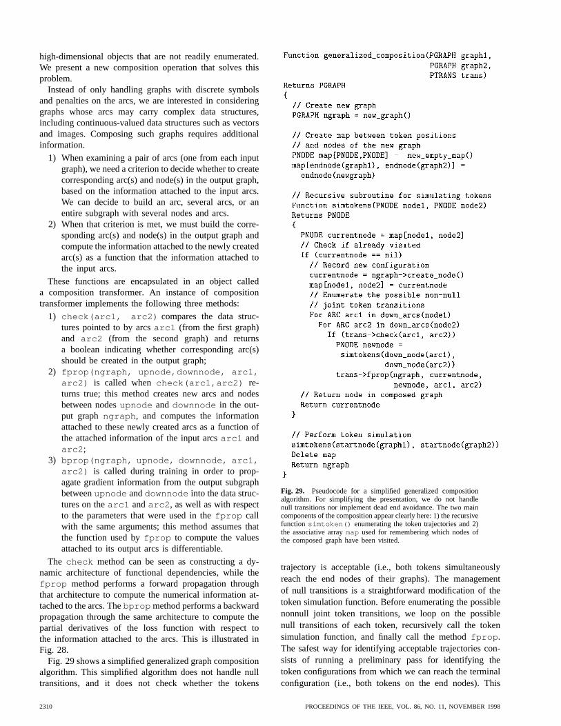
high-dimensional objects that are not readily enumerated.We present a new composition operation that solves thisproblem.

Instead of only handling graphs with discrete symbolsand penalties on the arcs, we are interested in consideringgraphs whose arcs may carry complex data structures,including continuous-valued data structures such as vectorsand images. Composing such graphs requires additionalinformation.

1) When examining a pair of arcs (one from each inputgraph), we need a criterion to decide whether to createcorresponding arc(s) and node(s) in the output graph,based on the information attached to the input arcs.We can decide to build an arc, several arcs, or anentire subgraph with several nodes and arcs.

2) When that criterion is met, we must build the corre-sponding arc(s) and node(s) in the output graph andcompute the information attached to the newly createdarc(s) as a function that the information attached tothe input arcs.

These functions are encapsulated in an object calleda composition transformer. An instance of compositiontransformer implements the following three methods:

1) check(arc1, arc2) compares the data struc-tures pointed to by arcsarc1 (from the first graph)and arc2 (from the second graph) and returnsa boolean indicating whether corresponding arc(s)should be created in the output graph;

2) fprop(ngraph, upnode,downnode, arc1,arc2) is called whencheck(arc1,arc2) re-turns true; this method creates new arcs and nodesbetween nodesupnode and downnode in the out-put graphngraph , and computes the informationattached to these newly created arcs as a function ofthe attached information of the input arcsarc1 andarc2 ;

3) bprop(ngraph, upnode, downnode, arc1,arc2) is called during training in order to prop-agate gradient information from the output subgraphbetweenupnode anddownnode into the data struc-tures on thearc1 andarc2 , as well as with respectto the parameters that were used in thefprop callwith the same arguments; this method assumes thatthe function used byfprop to compute the valuesattached to its output arcs is differentiable.

The check method can be seen as constructing a dy-namic architecture of functional dependencies, while thefprop method performs a forward propagation throughthat architecture to compute the numerical information at-tached to the arcs. Thebprop method performs a backwardpropagation through the same architecture to compute thepartial derivatives of the loss function with respect tothe information attached to the arcs. This is illustrated inFig. 28.

Fig. 29 shows a simplified generalized graph compositionalgorithm. This simplified algorithm does not handle nulltransitions, and it does not check whether the tokens

Fig. 29. Pseudocode for a simplified generalized compositionalgorithm. For simplifying the presentation, we do not handlenull transitions nor implement dead end avoidance. The two maincomponents of the composition appear clearly here: 1) the recursivefunction simtoken() enumerating the token trajectories and 2)the associative arraymap used for remembering which nodes ofthe composed graph have been visited.

trajectory is acceptable (i.e., both tokens simultaneouslyreach the end nodes of their graphs). The managementof null transitions is a straightforward modification of thetoken simulation function. Before enumerating the possiblenonnull joint token transitions, we loop on the possiblenull transitions of each token, recursively call the tokensimulation function, and finally call the methodfprop .The safest way for identifying acceptable trajectories con-sists of running a preliminary pass for identifying thetoken configurations from which we can reach the terminalconfiguration (i.e., both tokens on the end nodes). This


is easily achieved by enumerating the trajectories in theopposite direction. We start on the end nodes and followthe arcs upstream. During the main pass, we only buildthe nodes that allow the tokens to reach the terminalconfiguration.

Graph composition using transducers (i.e., standard trans-duction) is easily and efficiently implemented as a gener-alized transduction. The methodcheck simply tests theequality of the input symbols on the two arcs, and themethod fprop creates a single arc whose symbol is theoutput symbol on the transducer’s arc.

The composition between pairs of graphs is particularlyuseful for incorporating linguistic constraints in a handwrit-ing recognizer. Examples of its use are given in the onlinehandwriting recognition system described in Section IX(and in the check reading system described in Section X).

In the rest of the paper, the term composition transformerwill denote a GT based on the generalized transductionsof multiple graphs. The concept of generalized transduc-tion is a very general one. In fact, many of the GT’sdescribed earlier in this paper, such as the segmenter andthe recognizer, can be formulated in terms of generalizedtransduction. In this case, the generalized transduction doesnot take two input graphs but a single input graph. Themethodfprop of the transformer may create several arcsor even a complete subgraph for each arc of the initialgraph. In fact the paircheck,fprop itself can be seenas procedurally defining a transducer.

In addition, it can be shown that the generalized trans-duction of a single graph is theoretically equivalent tothe standard composition of this graph with a particulartransducer graph. However, implementing the operation thisway may be very inefficient since the transducer can bevery complicated.

In practice, the graph produced by a generalized transduc-tion is represented procedurally in order to avoid buildingthe whole output graph (which may be huge when forexample the interpretation graph is composed with thegrammar graph). We only instantiate the nodes which arevisited by the search algorithm during recognition (e.g.,Viterbi). This strategy propagates the benefits of pruningalgorithms (e.g., beam search) in all the GTN’s.

D. Notes on the Graph Structures

Section VI discussed the idea of global training by back-propagating gradient through simple GT’s. Thebpropmethod is the basis of the back-propagation algorithm forgeneric GT’s. A generalized composition transformer canbe seen as dynamically establishing functional relation-ships between the numerical quantities on the input andoutput arcs. Once thecheck function has decided that arelationship should be established, thefprop function im-plements the numerical relationship. Thecheck functionestablishes the structure of the ephemeral network insidethe composition transformer.

Since fprop is assumed to be differentiable, gradientscan be back propagated through that structure. Most param-eters affect the scores stored on the arcs of the successive

graphs of the system. A few threshold parameters maydetermine whether an arc appears or not in the graph.Since nonexisting arcs are equivalent to arcs with very largepenalties, we only consider the case of parameters affectingthe penalties.

In the kind of systems we have discussed until now(and the application described in Section X), much of theknowledge about the structure of the graph that is producedby a GT is determined by the nature of the GT, but it mayalso depend on the value of the parameters and on the input.It may also be interesting to consider GT modules whichattempt to learn the structure of the output graph. This mightbe considered a combinatorial problem and not amenableto gradient-based learning, but a solution to this problem isto generate a large graph that contains the graph candidatesas subgraphs, and then select the appropriate subgraph.

E. GTN and HMM’s

GTN’s can be seen as a generalization and an extensionof HMM’s. On the one hand, the probabilistic interpretationcan be either kept (with penalties being log-probabilities),pushed to the final decision stage (with the difference ofthe constrained forward penalty and the unconstrained for-ward penalty being interpreted as negative log-probabilitiesof label sequences), or dropped altogether (the networkjust represents a decision surface for label sequences ininput space). On the other hand, GTN’s extend HMM’sby allowing to combine in a well-principled frameworkmultiple levels of processing, or multiple models (e.g.,Pereiraet al. have been using the transducer framework forstacking HMM’s representing different levels of processingin automatic speech recognition [86]).

Unfolding an HMM in time yields a graph that is verysimilar to our interpretation graph (at the final stage ofprocessing of the GTN, before Viterbi recognition). It hasnodes associated to each time stepand state in themodel. The penalty for an arc from tothen corresponds to the negative log-probability of emittingobserved data at position and going from state tostate in the time interval With this probabilisticinterpretation, the forward penalty is the negative logarithmof the likelihood of whole observed data sequence (giventhe model).

In Section VI we mentioned that the collapsing phe-nomenon can occur when nondiscriminative loss functionsare used to train NN’s/HMM hybrid systems. With classi-cal HMM’s with fixed preprocessing, this problem doesnot occur because the parameters of the emission andtransition probability models are forced to satisfy certainprobabilistic constraints: the sum or the integral of theprobabilities of a random variable over its possible valuesmust be one. Therefore, when the probability of certainevents is increased, the probability of other events mustautomatically be decreased. On the other hand, if theprobabilistic assumptions in an HMM (or other probabilisticmodel) are not realistic, discriminative training, discussedin Section VI, can improve performance as this has been


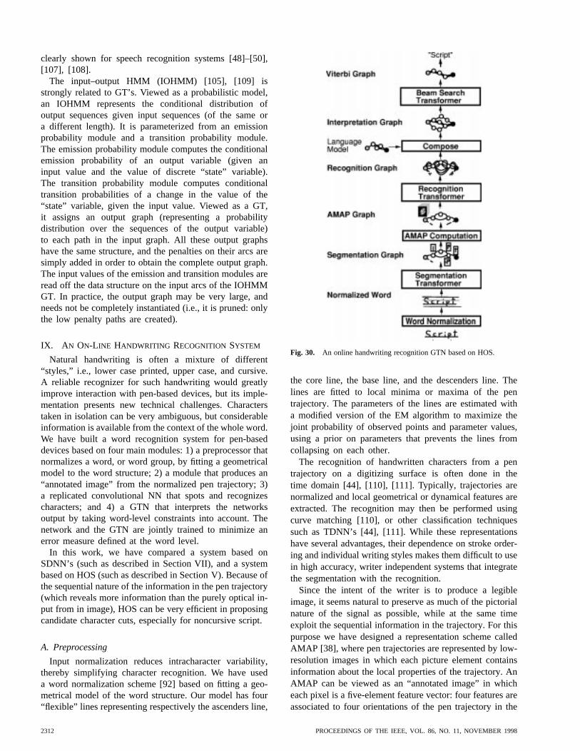
clearly shown for speech recognition systems [48]–[50],[107], [108].

The input–output HMM (IOHMM) [105], [109] isstrongly related to GT’s. Viewed as a probabilistic model,an IOHMM represents the conditional distribution ofoutput sequences given input sequences (of the same ora different length). It is parameterized from an emissionprobability module and a transition probability module.The emission probability module computes the conditionalemission probability of an output variable (given aninput value and the value of discrete “state” variable).The transition probability module computes conditionaltransition probabilities of a change in the value of the“state” variable, given the input value. Viewed as a GT,it assigns an output graph (representing a probabilitydistribution over the sequences of the output variable)to each path in the input graph. All these output graphshave the same structure, and the penalties on their arcs aresimply added in order to obtain the complete output graph.The input values of the emission and transition modules areread off the data structure on the input arcs of the IOHMMGT. In practice, the output graph may be very large, andneeds not be completely instantiated (i.e., it is pruned: onlythe low penalty paths are created).

IX. A N ON-LINE HANDWRITING RECOGNITION SYSTEM

Natural handwriting is often a mixture of different“styles,” i.e., lower case printed, upper case, and cursive.A reliable recognizer for such handwriting would greatlyimprove interaction with pen-based devices, but its imple-mentation presents new technical challenges. Characterstaken in isolation can be very ambiguous, but considerableinformation is available from the context of the whole word.We have built a word recognition system for pen-baseddevices based on four main modules: 1) a preprocessor thatnormalizes a word, or word group, by fitting a geometricalmodel to the word structure; 2) a module that produces an“annotated image” from the normalized pen trajectory; 3)a replicated convolutional NN that spots and recognizescharacters; and 4) a GTN that interprets the networksoutput by taking word-level constraints into account. Thenetwork and the GTN are jointly trained to minimize anerror measure defined at the word level.

In this work, we have compared a system based onSDNN’s (such as described in Section VII), and a systembased on HOS (such as described in Section V). Because ofthe sequential nature of the information in the pen trajectory(which reveals more information than the purely optical in-put from in image), HOS can be very efficient in proposingcandidate character cuts, especially for noncursive script.

A. Preprocessing

Input normalization reduces intracharacter variability,thereby simplifying character recognition. We have useda word normalization scheme [92] based on fitting a geo-metrical model of the word structure. Our model has four“flexible” lines representing respectively the ascenders line,

Fig. 30. An online handwriting recognition GTN based on HOS.

the core line, the base line, and the descenders line. Thelines are fitted to local minima or maxima of the pentrajectory. The parameters of the lines are estimated witha modified version of the EM algorithm to maximize thejoint probability of observed points and parameter values,using a prior on parameters that prevents the lines fromcollapsing on each other.

The recognition of handwritten characters from a pentrajectory on a digitizing surface is often done in thetime domain [44], [110], [111]. Typically, trajectories arenormalized and local geometrical or dynamical features areextracted. The recognition may then be performed usingcurve matching [110], or other classification techniquessuch as TDNN’s [44], [111]. While these representationshave several advantages, their dependence on stroke order-ing and individual writing styles makes them difficult to usein high accuracy, writer independent systems that integratethe segmentation with the recognition.

Since the intent of the writer is to produce a legibleimage, it seems natural to preserve as much of the pictorialnature of the signal as possible, while at the same timeexploit the sequential information in the trajectory. For thispurpose we have designed a representation scheme calledAMAP [38], where pen trajectories are represented by low-resolution images in which each picture element containsinformation about the local properties of the trajectory. AnAMAP can be viewed as an “annotated image” in whicheach pixel is a five-element feature vector: four features areassociated to four orientations of the pen trajectory in the


Fig. 31. An online handwriting recognition GTN based onSDNN.

area around the pixel and the fifth one is associated to localcurvature in the area around the pixel. A particularly usefulfeature of the AMAP representation is that it makes veryfew assumptions about the nature of the input trajectory.It does not depend on stroke ordering or writing speed,and it can be used with all types of handwriting (capital,lower case, cursive, punctuation, symbols). Unlike manyother representations (such as global features), AMAP’scan be computed for complete words without requiringsegmentation.

B. Network Architecture

One of the best networks we found for both online andoffline character recognition is a five-layer convolutionalnetwork somewhat similar to LeNet-5 (Fig. 2), but withmultiple input planes and different numbers of units onthe last two layers—layer one: convolution with eightkernels of size 3 3; layer two: 2 2 subsampling; layerthree: convolution with 25 kernels of size 55; layerfour: convolution with 84 kernels of size 44; layer five:2 1 subsampling; classification layer: 95 RBF units (oneper class in the full printable ASCII set). The distributedcodes on the output are the same as for LeNet-5, exceptthey are adaptive unlike with LeNet-5. When used in theHOS system, the input to above network consisted ofan AMAP with five planes, 20 rows, and 18 columns.It was determined that this resolution was sufficient forrepresenting handwritten characters. In the SDNN version,the number of columns was varied according to the width

of the input word. Once the number of subsampling layersand the sizes of the kernels are chosen, the sizes of all thelayers, including the input, are determined unambiguously.The only architectural parameters that remain to be selectedare the number of feature maps in each layer and the infor-mation as to what feature map is connected to what otherfeature map. In our case, the subsampling rates were chosenas small as possible (22) and the kernels as small aspossible in the first layer (33) to limit the total number ofconnections. Kernel sizes in the upper layers are chosen tobe as small as possible while satisfying the size constraintsmentioned above. Larger architectures did not necessarilyperform better and required considerably more time tobe trained. A very small architecture with half the inputfield also performed worse because of insufficient inputresolution. Note that the input resolution is nonethelessmuch less than for OCR because the angle and curvatureprovide more information than would a single grey levelat each pixel.

C. Network Training

Training proceeded in two phases. First, we kept thecenters of the RBF’s fixed and trained the network weightsso as to minimize the output distance of the RBF unitcorresponding to the correct class. This is equivalent tominimizing the MSE between the previous layer and thecenter of the correct-class RBF. This bootstrap phase wasperformed on isolated characters. In the second phase, allthe parameters, network weights, and RBF centers weretrained globally to minimize a discriminative criterion atthe word level.

With the HOS approach, the GTN was composed of fourmain GT’s.

1) Thesegmentation transformerperforms the HOS andoutputs the segmentation graph. An AMAP is thencomputed for each image attached to the arcs of thisgraph.

2) The character recognition transformerapplies theconvolutional network character recognizer to eachcandidate segment and outputs the recognition graphwith penalties and classes on each arc.

3) The composition transformercomposes the recog-nition graph with a grammar graph representing alanguage model incorporating lexical constraints.

4) The beam search transformerextracts a good in-terpretation from the interpretation graph. This taskcould have been achieved with the usual ViterbiTransformer. The beam search algorithm, however,implements pruning strategies which are appropriatefor large interpretation graphs.

With the SDNN approach, the main GT’s are the fol-lowing.

1) The SDNN transformerreplicates the convolutionalnetwork over the a whole word image and outputsa recognition graph that is a linear graph with class


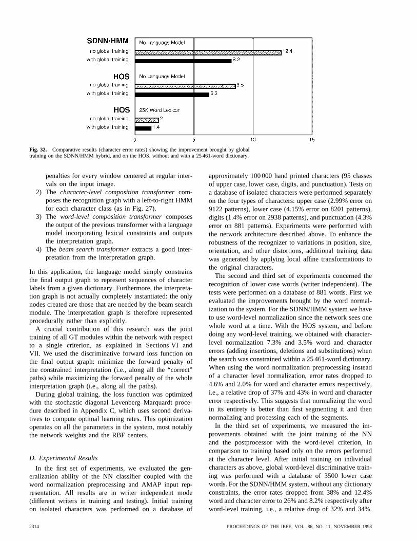
Fig. 32. Comparative results (character error rates) showing the improvement brought by globaltraining on the SDNN/HMM hybrid, and on the HOS, without and with a 25 461-word dictionary.

penalties for every window centered at regular inter-vals on the input image.

2) The character-level composition transformercom-poses the recognition graph with a left-to-right HMMfor each character class (as in Fig. 27).

3) The word-level composition transformercomposesthe output of the previous transformer with a languagemodel incorporating lexical constraints and outputsthe interpretation graph.

4) The beam search transformerextracts a good inter-pretation from the interpretation graph.

In this application, the language model simply constrainsthe final output graph to represent sequences of characterlabels from a given dictionary. Furthermore, the interpreta-tion graph is not actually completely instantiated: the onlynodes created are those that are needed by the beam searchmodule. The interpretation graph is therefore representedprocedurally rather than explicitly.

A crucial contribution of this research was the jointtraining of all GT modules within the network with respectto a single criterion, as explained in Sections VI andVII. We used the discriminative forward loss function onthe final output graph: minimize the forward penalty ofthe constrained interpretation (i.e., along all the “correct”paths) while maximizing the forward penalty of the wholeinterpretation graph (i.e., along all the paths).

During global training, the loss function was optimizedwith the stochastic diagonal Levenberg–Marquardt proce-dure described in Appendix C, which uses second deriva-tives to compute optimal learning rates. This optimizationoperates on all the parameters in the system, most notablythe network weights and the RBF centers.

D. Experimental Results

In the first set of experiments, we evaluated the gen-eralization ability of the NN classifier coupled with theword normalization preprocessing and AMAP input rep-resentation. All results are in writer independent mode(different writers in training and testing). Initial trainingon isolated characters was performed on a database of

approximately 100 000 hand printed characters (95 classesof upper case, lower case, digits, and punctuation). Tests ona database of isolated characters were performed separatelyon the four types of characters: upper case (2.99% error on9122 patterns), lower case (4.15% error on 8201 patterns),digits (1.4% error on 2938 patterns), and punctuation (4.3%error on 881 patterns). Experiments were performed withthe network architecture described above. To enhance therobustness of the recognizer to variations in position, size,orientation, and other distortions, additional training datawas generated by applying local affine transformations tothe original characters.

The second and third set of experiments concerned therecognition of lower case words (writer independent). Thetests were performed on a database of 881 words. First weevaluated the improvements brought by the word normal-ization to the system. For the SDNN/HMM system we haveto use word-level normalization since the network sees onewhole word at a time. With the HOS system, and beforedoing any word-level training, we obtained with character-level normalization 7.3% and 3.5% word and charactererrors (adding insertions, deletions and substitutions) whenthe search was constrained within a 25 461-word dictionary.When using the word normalization preprocessing insteadof a character level normalization, error rates dropped to4.6% and 2.0% for word and character errors respectively,i.e., a relative drop of 37% and 43% in word and charactererror respectively. This suggests that normalizing the wordin its entirety is better than first segmenting it and thennormalizing and processing each of the segments.

In the third set of experiments, we measured the im-provements obtained with the joint training of the NNand the postprocessor with the word-level criterion, incomparison to training based only on the errors performedat the character level. After initial training on individualcharacters as above, global word-level discriminative train-ing was performed with a database of 3500 lower casewords. For the SDNN/HMM system, without any dictionaryconstraints, the error rates dropped from 38% and 12.4%word and character error to 26% and 8.2% respectively afterword-level training, i.e., a relative drop of 32% and 34%.


For the HOS system and a slightly improved architecture,without any dictionary constraints, the error rates droppedfrom 22.5% and 8.5% word and character error to 17% and6.3% respectively, i.e., a relative drop of 24.4% and 25.6%.With a 25 461-word dictionary, errors dropped from 4.6%and 2.0% word and character errors to 3.2% and 1.4%,respectively, after word-level training, i.e., a relative dropof 30.4% and 30.0%. Even lower error rates can be obtainedby drastically reducing the size of the dictionary to 350words, yielding 1.6% and 0.94% word and character errors.

These results clearly demonstrate the usefulness of glob-ally trained NN/HMM hybrids for handwriting recognition.This confirms similar results obtained earlier in speechrecognition [77].

X. A CHECK READING SYSTEM

This section describes a GTN based check reading sys-tem, intended for immediate industrial deployment. It alsoshows how the use of gradient based-learning and GTN’smake this deployment fast and cost-effective while yieldingan accurate and reliable solution.

The verification of the amount on a check is a task thatis extremely time and money consuming for banks. Asa consequence, there is a very high interest in automat-ing the process as much as possible (see, for example,[112]–[114]). Even a partial automation would result inconsiderable cost reductions. The threshold of economicviability for automatic check readers, as set by the bank,is when 50% of the checks are read with less than 1%error. The other 50% of the check being rejected andsent to human operators. In such a case, we describe theperformance of the system as 50% correct/49% reject/1%error. The system presented here was one of the first tocross that threshold on representative mixtures of businessand personal checks.

Checks contain at least two versions of the amount. Thecourtesy amount is written with numerals, while the legalamount is written with letters. On business checks, whichare generally machine-printed, these amounts are relativelyeasy to read but quite difficult to find due to the lack ofstandard for business check layout. On the other hand, theseamounts on personal checks are easy to find but muchharder to read.

For simplicity (and speed requirements), our initial taskis to read the courtesy amount only. This task consists oftwo main steps.

1) The system has to find, among all the fields (linesof text), the candidates that are the most likely tocontain the courtesy amount. This is obvious for manypersonal checks, where the position of the amountis standardized. However, as already noted, findingthe amount can be rather difficult in business checks,even for the human eye. There are many strings ofdigits, such as the check number, the date, or even“not to exceed” amounts, that can be confused withthe actual amount. In many cases, it is very difficult todecide which candidate is the courtesy amount beforeperforming a full recognition.

Fig. 33. A complete check amount reader implemented as asingle cascade of GT modules. Successive graph transformationsprogressively extract higher level information.

2) In order to read (and choose) some courtesy amountcandidates, the system has to segment the fields intocharacters, read and score the candidate characters,and finally find the best interpretation of the amountusing contextual knowledge represented by a stochas-tic grammar for check amounts.

The GTN methodology was used to build a check amountreading system that handles both personal checks andbusiness checks.

A. A GTN for Check Amount Recognition

We now describe the successive graph transformationsthat allow this network to read the check amount (cf.Fig. 33). Each GT produces a graph whose paths encodeand score the current hypotheses considered at this stageof the system.

The input to the system is a trivial graph with a singlearc that carries the image of the whole check (cf. Fig. 33).

1) The Field Location Transformer: first performsclassical image analysis (including connected componentanalysis, ink density histograms, layout analysis, etc.) andheuristically extracts rectangular zones that may contain thecheck amount. produces an output graph, called thefield graph (cf. Fig. 33) such that each candidate zone isassociated with one arc that links the start node to theend node. Each arc contains the image of the zone anda penalty term computed from simple features extractedfrom the zone (absolute position, size, aspect ratio, etc.).The penalty term is close to zero if the features suggestthat the field is a likely candidate and is large if the field isdeemed less likely to be an amount. The penalty function isdifferentiable, therefore its parameters are globally tunable.


An arc may represent separate dollar and cent amountsas a sequence of fields. In fact, in handwritten checks, thecent amount may be written over a fractional bar and notaligned at all with the dollar amount. In the worst case, onemay find several cent amount candidates (above and belowthe fraction bar) for the same dollar amount.

2) The Segmentation Transformer: similar to theone described in Section VIII, examines each zonecontained in the field graph and cuts each image intopieces of ink using heuristic image processing techniques.Each piece of ink may be a whole character or a pieceof character. Each arc in the field graph is replaced byits corresponding segmentation graph that represents allpossible groupings of pieces of ink. Each field segmentationgraph is appended to an arc that contains the penalty of thefield in the field graph. Each arc carries the segment image,together with a penalty that provides a first evaluationof the likelihood that the segment actually contains acharacter. This penalty is obtained with a differentiablefunction that combines a few simple features such asthe space between the pieces of ink or the complianceof the segment image with a global baseline, and a fewtunable parameters. The segmentation graph represents allthe possible segmentations of all the field images. We cancompute the penalty for one segmented field by addingthe arc penalties along the corresponding path. As before,using a differentiable function for computing the penaltieswill ensure that the parameters can be optimized globally.

The segmenter uses a variety of heuristics to find candi-date cut. One of the most important ones is called “hit anddeflect” [115]. The idea is to cast lines downward from thetop of the field image. When a line hits a black pixel, it isdeflected so as to follow the contour of the object. When aline hits a local minimum of the upper profile, i.e., when itcannot continue downward without crossing a black pixel,it is just propagated vertically downward through the ink.When two such lines meet each other, they are mergedinto a single cut. The procedure can be repeated from thebottom up. This strategy allows the separation of touchingcharacters such as double zeros.

3) The Recognition Transformer: iterates over allsegment arcs in the segmentation graph and runs a characterrecognizer on the corresponding segment image. In ourcase, the recognizer is LeNet-5, the convolutional NNdescribed in Section II, whose weights constitute the largestand most important subset of tunable parameters. Therecognizer classifies segment images into one of 95 classes(fully printable ASCII set) plus a rubbish class for unknownsymbols or badly formed characters. Each arc in the inputgraph is replaced by 96 arcs in the output graph.Each of those 96 arcs contains the label of one of theclasses, and a penalty that is the sum of the penalty ofthe corresponding arc in the input (segmentation) graph,and the penalty associated with classifying the image inthe corresponding class, as computed by the recognizer. Inother words, the recognition graph represents a weightedtrellis of scored character classes. Each path in this graphrepresents a possible character string for the corresponding

field. We can compute a penalty for this interpretationby adding the penalties along the path. This sequence ofcharacters may or may not be a valid check amount.

4) The Composition Transformer: selects the pathsof the recognition graph that represent valid charactersequences for check amounts. This transformer takes twographs as input: the recognition graph and the grammargraph. The grammar graph contains all possible sequencesof symbols that constitute a well-formed amount. The out-put of the composition transformer, called the interpretationgraph, contains all the paths in the recognition graph that arecompatible with the grammar. The operation that combinesthe two input graphs to produce the output is a generalizedtransduction (see Section IX). A differentiable function isused to compute the data attached to the output arc fromthe data attached to the input arcs. In our case, the outputarc receives the class label of the two arcs and a penaltycomputed by simply summing the penalties of the twoinput arcs (the recognizer penalty and the arc penalty inthe grammar graph). Each path in the interpretation graphrepresents one interpretation of one segmentation of onefield on the check. The sum of the penalties along the pathrepresents the “badness” of the corresponding interpretationand combines evidence from each of the modules along theprocess, as well as from the grammar.

5) The Viterbi Transformer:The Viterbi transformer fi-nally selects the path with the lowest accumulated penaltycorresponding to the best grammatically correct interpreta-tions.

B. Gradient-Based Learning

Each stage of this check reading system contains tunableparameters. While some of these parameters could bemanually adjusted (e.g., the parameters of the field locatorand segmenter), the vast majority of them must be learned,particularly the weights of the NN recognizer.

Prior to globally optimizing the system, each module pa-rameters are initialized with reasonable values. The param-eters of the field locator and the segmenter are initialized byhand, while the parameters of the NN character recognizerare initialized by training on a database of presegmentedand labeled characters. Then, the entire system is trainedglobally from whole check images labeled with the correctamount. No explicit segmentation of the amounts is neededto train the system: it is trained at the check level.

The loss function minimized by our global trainingprocedure is the discriminative forward criterion describedin Section VI: the difference between 1) the forward penaltyof the constrained interpretation graph (constrained by thecorrect label sequence) and 2) the forward penalty of theunconstrained interpretation graph. Derivatives can be backpropagated through the entire structure, although it is onlypractical to do it down to the segmenter.

C. Rejecting Low Confidence Checks

In order to be able to reject checks which are themost likely to carry erroneous Viterbi answers, we mustrate them with a confidence and reject the check if this


Fig. 34. Additional processing required to compute the confi-dence.

confidence is below a given threshold. To compare theunnormalized Viterbi penalties of two different checkswould be meaningless when it comes to decide whichanswer we trust the most.

The optimal measure of confidence is the probabilityof the Viterbi answer given the input image. As seenin Section VI-E, given a target sequence (which, in thiscase, would be the Viterbi answer), the discriminativeforward loss function is an estimate of the logarithm ofthis probability. Therefore, a simple solution to obtain agood estimate of the confidence is to reuse the interpretationgraph (see Fig. 33) to compute the discriminative forwardloss as described in Fig. 21, using as our desired sequencethe Viterbi answer. This is summarized in Fig. 34, with

D. Results

A version of the above system was fully implementedand tested on machine-print business checks. This system isbasically a generic GTN engine with task specific heuristicsencapsulated in thecheck and fprop method. As a con-sequence, the amount of code to write was minimal: mostlythe adaptation of an earlier segmenter into the segmentationtransformer. The system that deals with handwritten orpersonal checks was based on earlier implementations thatused the GTN concept in a restricted way.

The NN classifier was initially trained on 500 000 imagesof character images from various origins spanning the entireprintable ASCII set. This contained both handwritten andmachine-printed characters that had been previously sizenormalized at the string level. Additional images weregenerated by randomly distorting the original images usingsimple affine transformations of the images. The networkwas then further trained on character images that had beenautomatically segmented from check images and manuallytruthed. The network was also initially trained to rejectnoncharacters that resulted from segmentation errors. Therecognizer was then inserted in the check-reading systemand a small subset of the parameters were trained globally(at the field level) on whole check images.

On 646 business checks that were automatically cat-egorized as machine printed, the performance was 82%correctly recognized checks, 1% errors, and 17% rejects.This can be compared to the performance of the previoussystem on the same test set: 68% correct, 1% errors, and31% rejects. A check is categorized as machine-printedwhen characters that are near a standard position dollarsign are detected as machine printed, or when, if nothing isfound in the standard position, at least one courtesy amountcandidate is found somewhere else. The improvement isattributed to three main causes. First the NN recognizerwas bigger and trained on more data. Second, because ofthe GTN architecture, the new system could take advantageof grammatical constraints in a much more efficient waythan the previous system. Third, the GTN architectureprovided extreme flexibility for testing heuristics, adjustingparameters, and tuning the system. This last point is moreimportant than it seems. The GTN framework separatesthe “algorithmic” part of the system from the “knowledge-based” part of the system, allowing easy adjustments of thelatter. The importance of global training was only minorin this task because the global training only concerned asmall subset of the parameters.

An independent test performed by systems integratorsin 1995 showed the superiority of this system over othercommercial courtesy amount reading systems. The systemwas integrated in NCR’s line of check reading systems. Ithas been fielded in several banks across the United Statessince June 1996, and it has been reading millions of checksper day since then.

XI. CONCLUSIONS

During the short history of automatic pattern recognition,increasing the role of learning seems to have invariablyimproved the overall performance of recognition systems.The systems described in this paper are more evidence tothis fact. Convolutional NN’s have been shown to eliminatethe need for hand-crafted feature extractors. GTN’s havebeen shown to reduce the need for hand-crafted heuristics,manual labeling, and manual parameter tuning in documentrecognition systems. As training data becomes plentiful, ascomputers get faster, and as our understanding of learningalgorithms improves, recognition systems will rely moreand more of learning and their performance will improve.

Just as the back-propagation algorithm elegantly solvedthe credit assignment problem in multilayer NN’s, thegradient-based learning procedure for GTN’s introduced inthis paper solves the credit assignment problem in systemswhose functional architecture dynamically changes witheach new input. The learning algorithms presented here arein a sense nothing more than unusual forms of gradientdescent in complex, dynamic architectures, with efficientback-propagation algorithms to compute the gradient. Theresults in this paper help establish the usefulness andrelevance of gradient-based minimization methods as ageneral organizing principle for learning in large systems.

It was shown that all the steps of a document analysissystem can be formulated as GT’s through which gradi-


ents can be back propagated. Even in the nontrainableparts of the system, the design philosophy in terms ofgraph transformation provides a clear separation betweendomain-specific heuristics (e.g., segmentation heuristics)and generic, procedural knowledge (the generalized trans-duction algorithm)

It is worth pointing out that data generating models (suchas HMM’s) and the maximum likelihood principle were notcalled upon to justify most of the architectures and the train-ing criteria described in this paper. Gradient-based learningapplied to global discriminative loss functions guaranteesoptimal classification and rejection without the use of “hardto justify” principles that put strong constraints on thesystem architecture, often at the expense of performances.

More specifically, the methods and architectures pre-sented in this paper offer generic solutions to a large numberof problems encountered in pattern recognition systems.

1) Feature extraction is traditionally a fixed transform,and it is generally derived from some expert priorknowledge about the task. This relies on the probablyincorrect assumption that the human designer is ableto capture all the relevant information in the input.We have shown that the application of gradient-basedlearning to convolutional NN’s allows us to learn ap-propriate features from examples. The success of thisapproach was demonstrated in extensive comparativedigit recognition experiments on the NIST database.

2) Segmentation and recognition of objects in imagescannot be completely decoupled. Instead of takinghard segmentation decisions too early, we have usedHOS to generate and evaluate a large number ofhypotheses in parallel, postponing any decision untilthe overall criterion is minimized.

3) Hand-truthing images to obtain segmented charactersfor training a character recognizer is expensive anddoes not take into account the way in which a wholedocument or sequence of characters will be recog-nized (in particular, the fact that some segmentationcandidates may be wrong, even though they may looklike true characters). Instead we train multimodulesystems to optimize a global measure of performance,which does not require time consuming detailed hand-truthing and yields significantly better recognitionperformance because it allows to train these modulesto cooperate toward a common goal.

4) Ambiguities inherent in the segmentation, characterrecognition, and linguistic model should be inte-grated optimally. Instead of using a sequence of task-dependent heuristics to combine these sources of in-formation, we have proposed a unified framework inwhich generalized transduction methods are appliedto graphs representing a weighted set of hypothesesabout the input. The success of this approach wasdemonstrated with a commercially deployed check-reading system that reads millions of business andpersonal checks per day: the generalized transductionengine resides in only a few hundred lines of code.

5) Traditional recognition systems rely on many hand-crafted heuristics to isolate individually recognizableobjects. The promising SDNN approach draws on therobustness and efficiency of convolutional NN’s toavoid explicit segmentation altogether. Simultaneousautomatic learning of segmentation and recognitioncan be achieved with gradient-based learning meth-ods.

This paper presents a small number of examples of GTmodules, but it is clear that the concept can be applied tomany situations where the domain knowledge or the stateinformation can be represented by graphs. This is the casein many audio signal recognition tasks, and visual sceneanalysis applications. Future work will attempt to applyGT networks to such problems, with the hope of allowingmore reliance on automatic learning and less on detailedengineering.

APPENDIX APRECONDITIONS FORFASTER CONVERGENCE

As seen before, the squashing function used in ourconvolutional networks is Symmetricfunctions are believed to yield faster convergence, althoughthe learning can become extremely slow if the weightsare too small. The cause of this problem is that in weightspace the origin is a fixed point of the learning dynamicsand, although it is a saddle point, it is attractive in almostall directions [116]. For our simulations, we use

and (see [20], [34]). With this choice ofparameters, the equalities and aresatisfied. The rationale behind this is that the overall gainof the squashing transformation is around one in normaloperating conditions, and the interpretation of the state ofthe network is simplified. Moreover, the absolute value ofthe second derivative of is a maximum at 1 and 1,which improves the convergence toward the end of thelearning session. This particular choice of parameters ismerely a convenience, and does not affect the result.

Before training, the weights are initialized with randomvalues using a uniform distribution between and

, where is the number of inputs (fan-in) of the unitwhich the connection belongs to. Since several connectionsshare a weight, this rule could be difficult to apply, but inour case all connections sharing a same weight belong tounits with identical fan-ins. The reason for dividing by thefan-in is that we would like the initial standard deviationof the weighted sums to be in the same range for eachunit and to fall within the normal operating region of thesigmoid. If the initial weights are too small, the gradientsare very small and the learning is slow. If they are toolarge, the sigmoids are saturated and the gradient is alsovery small. The standard deviation of the weighted sumscales like the square root of the number of inputs whenthe inputs are independent, and it scales linearly with thenumber of inputs if the inputs are highly correlated. Wechose to assume the second hypothesis since some unitsreceive highly correlated signals.


APPENDIX BSTOCHASTIC GRADIENT VERSUSBATCH GRADIENT

Gradient-based learning algorithms can use one of twoclasses of methods to update the parameters. The firstmethod, dubbed “batch gradient,” is the classical one: thegradients are accumulated over the entire training set, andthe parameters are updated after the exact gradient hasbeen so computed. In the second method, called “stochasticgradient,” a partial, or noisy, gradient is evaluated on thebasis of one single training sample (or a small numberof samples), and the parameters are updated using thisapproximate gradient. The training samples can be selectedrandomly or according to a properly randomized sequence.In the stochastic version the gradient estimates are noisy,but the parameters are updated much more often thanwith the batch version. An empirical result of considerablepractical importance is that on tasks with large, redundantdata sets, the stochastic version is considerably faster thanthe batch version, sometimes by orders of magnitude [117].Although the reasons for this are not totally understoodtheoretically, an intuitive explanation can be found in thefollowing extreme example. Let us take an example wherethe training database is composed of two copies of thesame subset. Then accumulating the gradient over the wholeset would cause redundant computations to be performed.On the other hand, running Stochastic Gradient once onthis training set would amount to performing two completelearning iterations over the small subset. This idea can begeneralized to training sets where there exist no preciserepetition of the same pattern but where some redundancy ispresent. In fact stochastic update must be better when thereis redundancy, i.e., when a certain level of generalizationis expected.

Many authors have claimed that second-order methodsshould be used in lieu of gradient descent for NN training.The literature abounds with recommendations [118] forclassical second-order methods such as the Gauss–Newtonor Levenberg–Marquardt algorithms for quasi-Newtonmethods such as Broyden–Fletcher–Goldfarb–Shanno,limited-storage Broyden–Fletcher–Goldfarb–Shanno, orfor various versions of the conjugate gradients method.Unfortunately, all of the above methods are unsuit-able for training large NN’s on large data sets. TheGauss–Newton and Levenberg–Marquardt methods require

operations per update, where is the numberof parameters, which makes them impractical for evenmoderate size networks. Quasi-Newton methods require“only” operations per update, but that still makesthem impractical for large networks. Limited-storage Broy-den–Fletcher–Goldfarb–Shanno’s and conjugate gradientsrequire only operations per update so they wouldappear appropriate. Unfortunately, their convergence speedrelies on an accurate evaluation of successive “conjugatedescent directions” which only makes sense in “batch”mode. For large data sets, the speed-up brought bythese methods over regular batch gradient descent cannotmatch the enormous speed up brought by the use of

stochastic gradient. Several authors have attempted touse conjugate gradient with small batches or batches ofincreasing sizes [119], [120], but those attempts havenot yet been demonstrated to surpass a carefully tunedstochastic gradient. Our experiments were performed witha stochastic method that scales the parameter axes so as tominimize the eccentricity of the error surface.

APPENDIX CSTOCHASTIC DIAGONAL LEVENBERG–MARQUARDT

Owing to the reasons given in Appendix B, we preferto update the weights after each presentation of a singlepattern in accordance with stochastic update methods. Thepatterns are presented in a constant random order, and thetraining set is typically repeated 20 times.

Our update algorithm is dubbed the stochastic diagonalLevenberg–Marquardt method where an individual learningrate (step size) is computed for each parameter (weight)before each pass through the training set [20], [34], [121].These learning rates are computed using the diagonal termsof an estimate of the Gauss–Newton approximation tothe Hessian (second derivative) matrix. This algorithm isnot believed to bring a tremendous increase in learningspeed but it converges reliably without requiring extensiveadjustments of the learning parameters. It corrects majorill-conditioning of the loss function that are due to thepeculiarities of the network architecture and the trainingdata. The additional cost of using this procedure overstandard stochastic gradient descent is negligible.

At each learning iteration a particular parameter isupdated according to the following stochastic update rule:

(18)

where is the instantaneous loss function for patternIn convolutional NN’s, because of the weight sharing,

the partial derivative is the sum of the partialderivatives with respect to the connections that share theparameter

(19)

where is the connection weight from unitto unitis the set of unit index pairs such that the connectionbetween and share the parameter i.e.,

(20)

As stated previously, the step sizesare not constant butare function of the second derivative of the loss functionalong the axis

(21)

where is a hand-picked constant and is an estimateof the second derivative of the loss functionwith respectto The larger is, the smaller the weight update.The parameter prevents the step size from becoming too


large when the second derivative is small, very much likethe “model-trust” methods, and the Levenberg–Marquardtmethods in nonlinear optimization [8]. The exact formulato compute from the second derivatives with respectto the connection weights is

(22)

However, we make three approximations. The first approx-imation is to drop the off-diagonal terms of the Hessianwith respect to the connection weights in (22)

(23)

Naturally, the terms are the average over thetraining set of the local second derivatives

(24)

Those local second derivatives with respect to connectionweights can be computed from local second derivatives withrespect to the total input of the downstream unit

(25)

where is the state of unit and is the secondderivative of the instantaneous loss function with respect tothe total input to unit (denoted Interestingly, there isan efficient algorithm to compute those second derivativeswhich is very similar to the back-propagation procedureused to compute the first derivatives [20], [21]

(26)

Unfortunately, using those derivatives leads to well-knownproblems associated with every Newton-like algorithm:these terms can be negative and can cause the gradientalgorithm to move uphill instead of downhill. Therefore,our second approximation is a well-known trick calledthe Gauss–Newton approximation, which guarantees thatthe second derivative estimates are nonnegative. TheGauss–Newton approximation essentially ignores thenonlinearity of the estimated function (the NN, in our case),but not that of the loss function. The back propagationequation for Gauss-Newton approximations of the secondderivatives is

(27)

This is very similar to the formula for back propagating thefirst derivatives, except that the sigmoid’s derivative andthe weight values are squared. The right-hand side is a sumof products of nonnegative terms, therefore the left-handside term is nonnegative.

The third approximation we make is that we do not runthe average in (24) over the entire training set, but run iton a small subset of the training set instead. In additionthe re-estimation does not need to be done often since thesecond-order properties of the error surface change ratherslowly. In the experiments described in this paper, we re-estimate the on 500 patterns before each training passthrough the training set. Since the size of the training setis 60 000, the additional cost of re-estimating the isnegligible. The estimates are not particularly sensitive to theparticular subset of the training set used in the averaging.This seems to suggest that the second-order properties ofthe error surface are mainly determined by the structureof the network, rather than by the detailed statistics of thesamples. This algorithm is particularly useful for shared-weight networks because the weight sharing creates illconditioning of the error surface. Because of the sharing,one single parameter in the first few layers can havean enormous influence on the output. Consequently, thesecond derivative of the error with respect to this parametermay be very large, while it can be quite small for otherparameters elsewhere in the network. The above algorithmcompensates for that phenomenon.

Unlike most other second-order acceleration methods forback-propagation, the above method works in stochasticmode. It uses a diagonal approximation of the Hessian.Like the classical Levenberg–Marquardt algorithm, it usesa “safety” factor to prevent the step sizes from gettingtoo large if the second derivative estimates are small.Hence the method is called the stochastic diagonal Lev-enberg–Marquardt method.

ACKNOWLEDGMENT

Some of the systems described in this paper are the workof many researchers now at AT&T and Lucent Technolo-gies. In particular, C. Burges, C. Nohl, T. Cauble, and J.Bromley contributed much to the check reading system.Experimental results described in Section III include con-tributions by C. Burges, A. Brunot, C. Cortes, H. Drucker,L. Jackel, U. Muller, B. Scholkopf, and P. Simard. Theauthors wish to thank F. Pereira, V. Vapnik, J. Denker, andI. Guyon for helpful discussions, C. Stenard and R. Higginsfor providing the applications that motivated some of thiswork, and L. R. Rabiner and L. D. Jackel for relentlesssupport and encouragement.

REFERENCES

[1] R. O. Duda and P. E. Hart,Pattern Classification and SceneAnalysis. New York: Wiley, 1973.

[2] Y. LeCun, B. Boser, J. S. Denker, D. Henderson, R. E. Howard,W. Hubbard, and L. D. Jackel, “Backpropagation applied tohandwritten zip code recognition,”Neural Computation, vol. 1,no. 4, pp. 541–551, Winter 1989.

[3] S. Seung, H. Sompolinsky, and N. Tishby, “Statistical mechan-ics of learning from examples,”Phys. Rev. A, vol. 45, pp.6056–6091, 1992.

[4] V. N. Vapnik, E. Levin, and Y. LeCun, “Measuring the vc-dimension of a learning machine,”Neural Computation, vol. 6,no. 5, pp. 851–876, 1994.

[5] C. Cortes, L. Jackel, S. Solla, V. N. Vapnik, and J. Denker,“Learning curves: Asymptotic values and rate of convergence,”


in Advances in Neural Information Processing Systems 6, J. D.Cowan, G. Tesauro, and J. Alspector, Eds. San Mateo, CA:Morgan Kaufmann, 1994, pp. 327–334.

[6] V. N. Vapnik, The Nature of Statistical Learning Theory. NewYork: Springer, 1995.

[7] , Statistical Learning Theory. New York: Wiley, 1998.[8] W. H. Press, B. P. Flannery, S. A. Teukolsky, and W. T.

Vetterling,Numerical Recipes: The Art of Scientific Computing.Cambridge, UK: Cambridge Univ., 1986.

[9] S. I. Amari, “A theory of adaptive pattern classifiers,”IEEETrans. Electron. Comput., vol. EC-16, pp. 299–307, 1967.

[10] Y. Tsypkin, Adaptation and Learning in Automatic SystemsNew York: Academic, 1971.

[11] , Foundations of the Theory of Learning Systems. NewYork: Academic, 1973.

[12] M. Minsky and O. Selfridge, “Learning in random nets,” inProc. 4th London Symp. Information Theory, pp. 335–347, 1961.

[13] D. H. Ackley, G. E. Hinton, and T. J. Sejnowski, “A learningalgorithm for Boltzmann machines,”Cognitive Sci., vol. 9, pp.147–169, 1985.

[14] G. E. Hinton and T. J. Sejnowski, “Learning and relearningin Boltzmann machines,” inParallel Distributed Processing:Explorations in the Microstructure of Cognition. Volume 1:Foundations, D. E. Rumelhart and J. L. McClelland, Eds.Cambridge, MA: MIT, 1986.

[15] D. E. Rumelhart, G. E. Hinton, and R. J. Williams, “Learn-ing internal representations by error propagation,” inParallelDistributed Processing: Explorations in the Microstructure ofCognition, vol. I. Cambridge, MA: Bradford Books, 1986,pp. 318–362,

[16] A. E. Bryson, Jr. and Y.-C. Ho,Applied Optimal Control.London, UK: Blaisdell, 1969.

[17] Y. LeCun, “A learning scheme for asymmetric thresholdnetworks,” in Proc. Cognitiva ’85, Paris, France, 1985, pp.599–604.

[18] , “Learning processes in an asymmetric threshold net-work,” in Disordered Systems and Biological Organization, E.Bienenstock, F. Fogelman-Soulie, and G. Weisbuch, Eds. LesHouches, France: Springer-Verlag, 1986, pp. 233–240.

[19] D. B. Parker, “Learning-logic,” Sloan School Manage., MIT,Cambridge, MA, Tech. Rep., TR-47, Apr. 1985.

[20] Y. LeCun, Modeles Connexionnistes de l’Apprentissage (Con-nectionist Learning Models), Ph.D. dissertation, Universite P.et M. Curie (Paris 6), June 1987.

[21] , “A theoretical framework for back-propagation,” inProc.1988 Connectionist Models Summer School, D. Touretzky, G.Hinton, and T. Sejnowski, Eds. Pittsburgh, PA: CMU, MorganKaufmann, 1988, pp. 21–28.

[22] L. Bottou and P. Gallinari, “A framework for the cooperationof learning algorithms,” inAdvances in Neural InformationProcessing Systems, vol. 3, D. Touretzky and R. Lippmann,Eds. Denver, CO: Morgan Kaufmann, 1991.

[23] C. Y. Suen, C. Nadal, R. Legault, T. A. Mai, and L. Lam,“Computer recognition of unconstrained handwritten numerals,”Proc. IEEE, vol. 80, pp. 1162–1180, July 1992.

[24] S. N. Srihari, “High-performance reading machines,”Proc.IEEE., vol. 80, pp. 1120–1132, July 1992.

[25] Y. LeCun, L. D. Jackel, B. Boser, J. S. Denker, H. P. Graf,I. Guyon, D. Henderson, R. E. Howard, and W. Hubbard,“Handwritten digit recognition: Applications of neural net chipsand automatic learning,”IEEE Trans. Commun., vol. 37, pp.41–46, Nov. 1989.

[26] J. Keeler, D. Rumelhart, and W. K. Leow, “Integrated seg-mentation and recognition of hand-printed numerals,” inNeuralInformation Processing Systems, R. P. Lippmann, J. M. Moody,and D. S. Touretzky, Eds. San Mateo, CA: Morgan Kaufmann,vol. 3, pp. 557–563, 1991.

[27] O. Matan, C. J. C. Burges, Y. LeCun, and J. S. Denker, “Multi-digit recognition using a space displacement neural network,”vol. 4, in Neural Information Processing Systems, J. M. Moody,S. J. Hanson, and R. P. Lippman, Eds. San Mateo, CA:Morgan Kaufmann, 1992.

[28] L. R. Rabiner, “A tutorial on hidden Markov models andselected applications in speech recognition,”Proc. IEEE, vol.77, pp. 257–286, Feb. 1989.

[29] H. A. Bourland and N. Morgan,Connectionist Speech Recog-nition: A Hybrid Approach. Boston: Kluwer, 1994.

[30] D. H. Hubel and T. N. Wiesel, “Receptive fields, binocular in-

teraction, and functional architecture in the cat’s visual cortex,”J. Physiology (London), vol. 160, pp. 106–154, 1962.

[31] K. Fukushima, “Cognition: A self-organizing multilayered neu-ral network,” Biological Cybern., vol. 20, pp. 121–136, 1975.

[32] K. Fukushima and S. Miyake, “Neocognitron: A new algorithmfor pattern recognition tolerant of deformations and shifts inposition,” Pattern Recognit., vol. 15, no. 6, pp. 455–469, Nov.1982.

[33] M. C. Mozer, The Perception of Multiple Objects: A Con-nectionist Approach. Cambridge, MA: MIT-Bradford Books,1991.

[34] Y. LeCun, “Generalization and network design strategies,”in Connectionism in Perspective, R. Pfeifer, Z. Schreter, F.Fogelman, and L. Steels, Eds. Zurich, Switzerland: Elsevier,1989.

[35] Y. LeCun, B. Boser, J. S. Denker, D. Henderson, R. E.Howard, W. Hubbard, and L. D. Jackel, “Handwritten digitrecognition with a back-propagation network,” inAdvancesin Neural Information Processing Systems 2 (NIPS’89), DavidTouretzky, Ed. Denver, CO: Morgan Kaufmann, 1990.

[36] G. L. Martin, “Centered-object integrated segmentation andrecognition of overlapping hand-printed characters,”NeuralComputation, vol. 5, no. 3, pp. 419–429, 1993.

[37] J. Wang and J. Jean, “Multi-resolution neural networks foromnifont character recognition,” inProc. Int. Conf. NeuralNetworks, vol. III, 1993, pp. 1588–1593.

[38] Y. Bengio, Y. LeCun, C. Nohl, and C. Burges, “Lerec: ANN/HMM hybrid for on-line handwriting recognition,”NeuralComputation, vol. 7, no. 5, 1995.

[39] S. Lawrence, C. L. Giles, A. C. Tsoi, and A. D. Back, “Facerecognition: A convolutional neural network approach,”IEEETrans. Neural Networks, vol. 8, pp. 98–113, Jan. 1997.

[40] K. J. Lang and G. E. Hinton, “A time delay neural networkarchitecture for speech recognition,” Carnegie-Mellon Univ.,Pittsburgh, PA, Tech. Rep. CMU-CS-88-152, 1988.

[41] A. H. Waibel, T. Hanazawa, G. Hinton, K. Shikano, and K.Lang, “Phoneme recognition using time-delay neural networks,”IEEE Trans. Acoustics, Speech, Signal Processing, vol. 37, pp.328–339, Mar. 1989.

[42] L. Bottou, F. Fogelman, P. Blanchet, and J. S. Lienard, “Speakerindependent isolated digit recognition: Multilayer perceptronversus dynamic time warping,”Neural Networks, vol. 3, pp.453–465, 1990.

[43] P. Haffner and A. H. Waibel, “Time-delay neural networksembedding time alignment: A performance analysis,” inProc.EUROSPEECH’91, 2nd Europ. Conf. Speech Communicationand Technology, Genova, Italy.

[44] I. Guyon, P. Albrecht, Y. LeCun, J. S. Denker, and W. Hubbard,“Design of a neural network character recognizer for a touchterminal,” Pattern Recognit., vol. 24, no. 2, pp. 105–119, 1991.

[45] J. Bromley, J. W. Bentz, L. bottou, I. Guyon, Y. LeCun, C.Moore, E. Sackinger, and R. Shah, “Signature verification usinga siamese time delay neural network,”Int. J. Pattern Recognit.Artificial Intell., vol. 7, no. 4, pp. 669–687, Aug. 1993.

[46] Y. LeCun, I. Kanter, and S. Solla, “Eigenvalues of covariancematrices: Application to neural-network learning,”Phys. Rev.Lett., vol. 66, no. 18, pp. 2396–2399, May 1991.

[47] T. G. Dietterich and G. Bakiri, “Solving multiclass learningproblems via error-correcting output codes,”J. Artificial Intell.Res., vol. 2, pp. 263–286, 1995.

[48] L. R. Bahl, P. F. Brown, P. V. de Souza, and R. L. Mercer,“Maximum mutual information of hidden Markov model pa-rameters for speech recognition,” inProc. Int. Conf. Acoustics,Speech, Signal Processing, 1986, pp. 49–52.

[49] , “Speech recognition with continuous-parameter hiddenMarkov models,” Comput., Speech Language, vol. 2, pp.219–234, 1987.

[50] B. H. Juang and S. Katagiri, “Discriminative learning forminimum error classification,”IEEE Trans. Acoustics, Speech,Signal Processing, vol. 40, pp. 3043–3054, Dec. 1992.

[51] Y. LeCun, L. D. Jackel, L. Bottou, A. Brunot, C. Cortes, J. S.Denker, H. Drucker, I. Guyon, U. A. Muller, E. S¨ackinger, P.Simard, and V. N. Vapnik, “Comparison of learning algorithmsfor handwritten digit recognition,” inInt. Conf. Artificial NeuralNetworks, F. Fogelman and P. Gallinari, Eds. Paris: EC2 &Cie, 1995, pp. 53–60.

[52] I. Guyon, I. Poujaud, L. Personnaz, G. Dreyfus, J. Denker, andY. LeCun, “Comparing different neural net architectures for


classifying handwritten digits,” inProc. IEEE IJCNN, Wash-ington, DC, vol. II, 1989, pp. 127–132,.

[53] R. Ott, “Construction of quadratic polynomial classifiers,” inProc. IEEE Int. Conf. Pattern Recognition, 1976, pp. 161–165.

[54] J. Schurmann, “A multifont word recognition system for postaladdress reading,”IEEE Trans. Comput., vol. C-27, pp. 721–732,Aug. 1978.

[55] Y. Lee, “Handwritten digit recognition using k-nearest neigh-bor, radial-basis functions, and backpropagation neural net-works,” Neural Computation, vol. 3, no. 3, pp. 440–449, 1991.

[56] D. Saad and S. A. Solla, “Dynamics of on-line gradient descentlearning for multilayer neural networks,” inAdvances in NeuralInformation Processing Systems, vol. 8, D. S. Touretzky, M.C. Mozer, and M. E. Hasselmo, Eds. Cambridge, MA: MIT,1996, pp. 302–308.

[57] G. Cybenko, “Approximation by superpositions of sigmoidalfunctions,” Math. Control, Signals, Syst., vol. 2, no. 4, pp.303–314, 1989.

[58] L. Bottou and V. N. Vapnik, “Local learning algorithms,”Neural Computation, vol. 4, no. 6, pp. 888–900, 1992.

[59] R. E. Schapire, “The strength of weak learnability,”MachineLearning, vol. 5, no. 2, pp. 197–227, 1990.

[60] H. Drucker, R. Schapire, and P. Simard, “Improving per-formance inneural networks using a boosting algorithm,” inAdvances in Neural Information Processing Systems 5, S. J.Hanson, J. D. Cowan, and C. L. Giles, Eds. San Mateo, CA:Morgan Kaufmann, 1993, pp. 42–49.

[61] P. Simard, Y. LeCun, and J. Denker, “Efficient pattern recog-nition using a new transformation distance,” inAdvances inNeural Information Processing Systems, vol. 5, S. Hanson, J.Cowan, and L. Giles, Eds. San Mateo, CA: Morgan Kauf-mann, 1993.

[62] B. Boser, I. Guyon, and V. Vapnik, “A training algorithmfor optimal margin classifiers,” inProc. 5th Annu. WorkshopComputational Learning Theory, vol. 5, 1992, pp. 144–152.

[63] C. J. C. Burges and B. Schoelkopf, “Improving the accuracyand speed of support vector machines,” inAdvances in NeuralInformation Processing Systems 9, M. Jordan, M. Mozer, andT. Petsche, Eds. Cambridge, MA: MIT, 1997.

[64] E. Sackinger, B. Boser, J. Bromley, Y. LeCun, and L. D. Jackel,“Application of the ANNA neural network chip to high-speedcharacter recognition,”IEEE Trans. Neural Networks, vol. 3,no. 3, pp. 498–505, Mar. 1992.

[65] J. S. Bridle, “Probabilistic interpretation of feedforward classi-fication networks outputs, with relationship to statistical patternrecognition,” inNeurocomputing, Algorithms, Architectures andApplications, F. Fogelman, J. Herault, and Y. Burnod, Eds.Les Arcs, France: Springer, 1989.

[66] Y. LeCun, L. Bottou, and Y. Bengio, “Reading checks withgraph transformer networks,” inProc. IEEE Int. Conf. Acous-tics, Speech, Signal Processing. Munich, Germany, vol. 1, 1997,pp. 151–154,.

[67] Y. Bengio,Neural Networks for Speech and Sequence Recogni-tion. London, UK: International Thompson, 1996.

[68] C. Burges, O. Matan, Y. LeCun, J. Denker, L. Jackel, C.Stenard, C. Nohl, and J. Ben, “Shortest path segmentation: Amethod for training a neural network to recognize characterstrings,” in Proc. Int. Joint Conf. Neural Networks, Baltimore,MD, vol. 3, 1992, pp. 165–172.

[69] T. M. Breuel, “A system for the off-line recognition of hand-written text,” in Proc. IEEE ICPR’94, Jerusalem, pp. 129–134.

[70] A. Viterbi, “Error bounds for convolutional codes and anasymptotically optimum decoding algorithm,”IEEE Trans. In-form. Theory, vol. 15, pp. 260–269, Apr. 1967.

[71] R. P. Lippmann and B. Gold, “Neural-net classifiers usefulfor speech recognition,” inProc. IEEE 1st Int. Conf. NeuralNetworks, San Diego, CA, June 1987, pp. 417–422.

[72] H. Sakoe, R. Isotani, K. Yoshida, K. Iso, and T. Watan-abe, “Speaker-independent word recognition using dynamicprogramming neural networks,” inProc. Int. Conf. Acoustics,Speech, Signal Processing, Glasgow, 1989, pp. 29–32.

[73] J. S. Bridle, “Alphanets: A recurrent ‘neural’ network archi-tecture with a hidden Markov model interpretation,”SpeechCommun., vol. 9, no. 1, pp. 83–92, 1990.

[74] M. A. Franzini, K. F. Lee, and A. H. Waibel, “Connectionistviterbi training: A new hybrid method for continuous speechrecognition,” inProc. Int. Conf. Acoustics, Speech, Signal Pro-cessing, Albuquerque, NM, 1990, pp. 425–428.

[75] L. T. Niles and H. F. Silverman, “Combining hidden Markovmodels and neural network classifiers,” inProc. Int. Conf.Acoustics, Speech, Signal Processing, Albuquerque, NM, 1990,pp. 417–420.

[76] X. Driancourt and L. Bottou, “MLP, LVQ and DP: Comparison& cooperation,” in Proc. Int. Joint Conf. Neural Networks,Seattle, WA, vol. 2, 1991, pp. 815–819.

[77] Y. Bengio, R. De Mori, G. Flammia, and R. Kompe, “Globaloptimization of a neural network-hidden Markov model hybrid,”IEEE Trans. Neural Networks, vol. 3, pp. 252–259, March 1992.

[78] P. Haffner and A. H. Waibel, “Multi-state time-delay neural net-works for continuous speech recognition,” vol. 4, inAdvancesin Neural Information Processing Systems. San Mateo, CA:Morgan Kaufmann, pp. 579–588, 1992.

[79] Y. Bengio, P. Simard, and P. Frasconi, “Learning long-termdependencies with gradient descent is difficult,”IEEE Trans.Neural Networks, vol. 5, no. 2, pp. 157–166, Mar. 1994.

[80] T. Kohonen, G. Barna, and R. Chrisley, “Statistical patternrecognition with neural network: Benchmarking studies,” inProc. IEEE 2nd Int. Conf. Neural Networks, San Diego, CA,vol. 1, 1988, pp. 61–68.

[81] P. Haffner, “Connectionist speech recognition with a globalMMI algorithm,” in Proc. EUROSPEECH’93, 3rd Europ. Conf.Speech Communication and Technology, Berlin, pp. 1929–1932.

[82] J. S. Denker and C. J. Burges, “Image segmentation andrecognition,” inThe Mathematics of Induction. Reading, MA:Addison Wesley, 1995.

[83] L. Bottou,Une Approche théorique de l’Apprentissage Connex-ionniste: Applications à la Reconnaissance de la Parole, Ph.D.dissertation, Univ. Paris XI, France, 1991.

[84] M. Rahim, Y. Bengio, and Y. LeCun, “Disriminative featureand model design for automatic speech recognition,” inProc.Eurospeech, Rhodes, Greece, 1997, pp. 75–78.

[85] U. Bodenhausen, S. Manke, and A. Waibel, “Connectionistarchitectural learning for high performance character and speechrecognition,” inProc. Int. Conf. Acoustics, Speech, Signal Pro-cessing, Minneapolis, MN, vol. 1, 1993, pp. 625–628.

[86] F. Pereira, M. Riley, and R. Sproat, “Weighted rational trans-ductions and their application to human language processing,”in ARPA Natural Language Processing Workshop, 1994.

[87] M. Lades, J. C. Vorbruggen, J. Buhmann, and C. von der Mals-burg, “Distortion invariant object recognition in the dynamiclink architecture,”IEEE Trans. Comput., vol. 42, pp. 300–311,March 1993.

[88] B. Boser, E. Säckinger, J. Bromley, Y. LeCun, and L. Jackel,“An analog neural network processor with programmable topol-ogy,” IEEE J. Solid-State Circuits, vol. 26, pp. 2017–2025, Dec.1991.

[89] M. Schenkel, H. Weissman, I. Guyon, C. Nohl, and D. Hender-son, “Recognition-based segmentation of on-line hand-printedwords,” in Advances in Neural Information Processing Systems5, S. J. Hanson, J. D. Cowan, and C. L. Giles, Eds. Denver,CO: Morgan Kaufmann, 1993, pp. 723–730.

[90] C. Dugust, L. Devillers, and X. Aubert, “Combining TDNNand HMM in a hybrid system for improved continuous-speechrecognition,”IEEE Trans. Speech Audio Processing, vol. 2, pp.217–224, Jan. 1994.

[91] O. Matan, H. S. Baird, J. Bromley, C. J. C. Burges, J. S. Denker,L. D. Jackel, Y. LeCun, E. P. D. Pednault, W. Satterfield, C. E.Stenard, and T. J. Thompson, “Reading handwritten digits: AZIP code recognition system,”IEEE Trans. Comput., vol. 25,no. 7, pp. 59–63, July 1992.

[92] Y. Bengio and Y. LeCun, “Word normalization for on-linehandwritten word recognition,” inProc. IEEE Int. Conf. PatternRecognition, Jerusalem, 1994.

[93] R. Vaillant, C. Monrocq, and Y. LeCun, “Original approach forthe localization of objects in images,”Proc. Inst. Elect. Eng.,vol. 141, no. 4, pp. 245–250, Aug. 1994.

[94] R. Wolf and J. Platt, “Postal address block location using aconvolutional locator network,” inAdvances in Neural Infor-mation Processing Systems 6, J. D. Cowan, G. Tesauro, andJ. Alspector, Eds. San Mateo, CA: Morgan Kaufmann, 1994,pp. 745–752.

[95] S. Nowlan and J. Platt, “A convolutional neural network handtracker,” inAdvances in Neural Information Processing Systems7, G. Tesauro, D. Touretzky, and T. Leen, Eds. San Mateo,CA: Morgan Kaufmann, 1995, pp. 901–908.

[96] H. A. Rowley, S. Baluja, and T. Kanade, “Neural network-based


face detection,” inProc. IEEE CVPR’96, pp. 203–208.[97] E. Osuna, R. Freund, and F. Girosi, “Training support vector

machines: An application to face detection,” inProc. IEEECVPR’96, pp. 130–136.

[98] H. Bourlard and C. J. Wellekens, “Links between Markovmodels and multilayer perceptrons,” inAdvances in NeuralInformation Processing Systems, D. Touretzky, Ed. Denver:Morgan-Kaufmann, vol. 1, 1989, pp. 186–187.

[99] Y. Bengio, R. De Mori, G. Flammia, and R. Kompe, “Neuralnetwork—Gaussian mixture hybrid for speech recognition ordensity estimation,” inAdvances in Neural Information Process-ing Systems 4, J. E. Moody, S. J. Hanson, and R. P. Lippmann,Eds. Denver, CO: Morgan Kaufmann, 1992, pp. 175–182.

[100] F. C. N. Pereira and M. Riley, “Speech recognition by compo-sition of weighted finite automata,” inFinite-State Devices forNatural Lague Processing. Cambridge, MA: MIT, 1997.

[101] M. Mohri, “Finite-state transducers in language and speechprocessing,”Computational Linguistics, vol. 23, no. 2, pp.269–311, 1997.

[102] I. Guyon, M. Schenkel, and J. Denker, “Overview and syn-thesis of on-line cursive handwriting recognition techniques,”in Handbook on Optical Character Recognition and DocumentImage Analysis, P. S. P. Wang and H. Bunke, Eds. New York:World Scientific, 1996.

[103] M. Mohri and M. Riley, “Weighted determinization and mini-mization for large vocabulary recognition,” inProc. Eurospeech’97, Rhodes, Greece, pp. 131–134.

[104] Y. Bengio and P. Frasconi, “An input/output HMM architec-ture,” in Advances in Neural Information Processing Systems,vol. 7, G. Tesauro, D. Touretzky, and T. Leen, Eds. Cam-bridge, MA: MIT, pp. 427–434, 1996.

[105] , “Input/output HMM’s for sequence processing,”IEEETrans. Neural Networks, vol. 7, no. 5, pp. 1231–1249, 1996.

[106] M. Mohri, F. C. N. Pereira, and M. Riley,A Rational Designfor a Weighted Finite-State Transducer Library(Lecture Notesin Computer Science). New York: Springer Verlag, 1997.

[107] M. Rahim, C. H. Lee, and B. H. Juang, “Discriminativeutterance verification for connected digits recognition,”IEEETrans. Speech Audio Processing, vol. 5, pp. 266–277, 1997.

[108] M. Rahim, Y. Bengio, and Y. LeCun, “Discriminative featureand model design for automatic speech recognition,” inProc.Eurospeech ’97, Rhodes, Greece.

[109] S. Bengio and Y. Bengio, “An EM algorithm for asynchronousinput/output hidden Markov models,” inProc. InternationalConference on Neural Information Processing, Hong-King,1996, pp. 328–334.

[110] C. Tappert, C. Suen, and T. Wakahara, “The state of the artin on-line handwriting recognition,”IEEE Trans. Pattern Anal.Machine Intell., vol. 8, pp. 787–808, Dec. 1990.

[111] S. Manke and U. Bodenhausen, “A connectionist recognizerfor on-line cursive handwriting recognition,” inProc. Int. Conf.Acoustics, Speech, Signal Processing, Adelaide, vol. 2, 1994,pp. 633–636.

[112] M. Gilloux and M. Leroux, “Recognition of cursive scriptamounts on postal checks,” inProc. Europ. Conf. Postal Tech-nol., Nantes, France, June 1993, pp. 705–712.

[113] D. Guillevic and C. Y. Suen, “Cursive script recognition appliedto the processing of bank checks,” inProc. Int. Conf. DocumentAnalysis Recognition, Montreal, Canada, Aug. 1995, pp. 11–14.

[114] L. Lam, C. Y. Suen, D. Guillevic, N. W. Strathy, M. Cheriet,K. Liu, and J. N. Said, “Automatic processing of informa-tion on checks,” inInt. Conf. Systems, Man, and Cybernetics,Vancouver, Canada, Oct. 1995, pp. 2353–2358.

[115] C. J. C. Burges, J. I. Ben, J. S. Denker, Y. LeCun, and C. R.Nohl, “Off line recognition of handwritten postal words usingneural networks,”Int. J. Pattern Recognit. Artificial Intell., vol.7, no. 4, p. 689, 1993.

[116] Y. LeCun, Y. Bengio, D. Henderson, A. Weisbuch, H. Weiss-man, and L. Jackel, “On-line handwriting recognition withneural networks: Spatial representation versus temporal repre-sentation,” inProc. Int. Conf. Handwriting Drawing, 1993.

[117] U. Muller, A. Gunzinger, and W. Guggenbühl, “Fast neural netsimulation with a DSP processor array,”IEEE Trans. NeuralNetworks, vol. 6, pp. 203–213, Jan. 1995.

[118] R. Battiti, “First- and second-order methods for learning: Be-tween steepest descent and Newton’s method,”Neural Compu-tation, vol. 4, no. 2, pp. 141–166, 1992.

[119] A. H. Kramer and A. Sangiovanni-Vincentelli, “Efficient par-

allel learning algorithms for neural networks,” inAdvances inNeural Information Processing Systems, vol. 1, D. S. Touretzky,Ed. San Mateo, CA: Morgan Kaufmann, 1988, pp. 40–48.

[120] M. Moller, Efficient Training of Feed-Forward Neural Net-works, Ph.D. dissertation, Aarhus Univ., Aarhus, Denmark,1993.

[121] S. Becker and Y. LeCun, “Improving the convergence ofback-propagation learning with second-order methods,” Univ.Toronto Connectionist Res. Group, Toronto, Ontario, Canada,Tech. Rep. CRG-TR-88-5, Sept. 1988.

Yann LeCun (Member, IEEE) received theDiplome d’Ingenieur degree from the EcoleSuperieure d’Ingenieur en Electrotechniqueet Electronique, Paris, in 1983 and the Ph.D.degree in computer science from the UniversitéPierre et Marie Curie, Paris, in 1987.

During his time at the Universite Pierre etMarie Curie, he proposed an early version ofthe back-propagation learning algorithm forneural networks. He joined the Department ofComputer Science at the University of Toronto,

Toronto, Ont., Canada, as a Research Associate in 1987. In 1988, he joinedthe Adaptive Systems Research Department at AT&T Bell Laboratories,Holmdel, NJ, where he worked on neural networks, machine learning, andhandwriting recognition. In 1996 he became Head of the Image ProcessingServices Research Department at AT&T Labs-Research, Red Bank, NJ.He has published over 70 technical papers and book chapters on neuralnetworks, machine learning, pattern recognition, handwriting recognition,document understanding, image processing, very large scale integration(VLSI) design, and information theory. In addition to the above topics, hiscurrent interests include video-based user interfaces, image compression,and content-based indexing of multimedia material.

Dr. LeCun serves on the board of theMachine Learning Journalandhas served as Associate Editor of the IEEE TRANSACTIONS ON NEURAL

NETWORKS. He is General Chair of the “Machines That Learn” workshop,which has been held every year since 1986 in Snowbird, UT. He hasserved as Program Co-Chair of IJCNN’89, INNC’90, and NIPS’90,’94, and ’95. He is a member of the IEEE Neural Network for SignalProcessing Technical Committee.

Leon Bottou received the Dipome degree fromEcole Polytechnique, Paris, in 1987, the Mag-istere en Mathematiques Fondamentales et Ap-pliquees et Informatiques degree from EcoleNormale Superieure, Paris in 1988, and thePh.D. degree in computer science from Univer-site de Paris-Sud in 1991.

During his time at Université de Paris-Sud heworked on speech recognition and proposed aframework for stochastic gradient learning andglobal training. He then joined the Adaptive

Systems Research Department at AT&T Bell Laboratories, Holmdel, NJ,where he worked on neural networks, statistical learning theory, and locallearning algorithms. He returned to France in 1992 as a Research Engineerat ONERA. He then became Chairman of Neuristique S.A., a companythat makes neural network simulators and traffic forecasting software.He returned to AT&T Bell Laboratories in 1995 where he worked ongraph transformer networks for optical character recognition. He is now aMember of the Image Processing Services Research Department at AT&TLabs-Research, Red Bank, NJ. Besides learning algorithms, his currentinterests include arithmetic coding, image compression, and indexing.


Yoshua Bengioreceived the B.Eng. degree inelectrical engineering and the M.Sc. and Ph.D.degrees in computer science from McGill Uni-versity, Montreal, P.Q., Canada, in 1986, 1988,and 1991, respectively.

In 1991–1992 he was a Postdoctoral Fel-low at the Massachusetts Institute of Technol-ogy, Cambridge. In 1992 he joined AT&T BellLaboratories, which later became AT&T Labs-Research, Red Bank, NJ. In 1993 he joined thefaculty of the computer science department of

the Universite de Montreal, Montreal, P.Q., Canada, where he is now anAssociate Professor. Since his first work on neural networks in 1986,his research interests have been centered around learning algorithms,especially for data with a sequential or spatial nature, such as speech,handwriting, and time-series.

Patrick Haffner graduated from Ecole Poly-technique, Paris, in 1987 and from EcoleNationale Superieure des Telecommunications(ENST), Paris, in 1989. He received the Ph.Ddegree in speech and signal processing fromENST in 1994.

In 1988 and 1990, he worked on the design ofthe TDNN and the MS-TDNN architectures atATR (Japan) and Carnegie Mellon University.From 1989 to 1995, as a Research Scientistfor CNET/France-T´elecom in Lannion, France,

he developed connectionist learning algorithms for telephone speechrecognition. In 1995, he joined AT&T Bell Laboratories, Holmdel, NJ, andworked on the application of optical character recognition and transducersto the processing of financial documents. In 1997, he joined the ImageProcessing Services Research Department at AT&T Labs-Research, RedBank, NJ. His research interests include statistical and connectionistmodels for sequence recognition, machine learning, speech and imagerecognition, and information theory.


gradient-based learning applied to document recognition · gradient-based learning applied to...

Documents