Grade/CPN: A Tool and Temporal Logic forTesting Colored Petri Net Models in Teaching

Michael Westergaard1,2?, Dirk Fahland1, and Christian Stahl1

1 Department of Mathematics and Computer Science,Eindhoven University of Technology, The Netherlands

{m.westergaard,d.fahland,c.stahl}@tue.nl2 National Research University Higher School of Economics,

Moscow, 101000, Russia

Abstract. Grading dozens of Petri net models manually is a tedious anderror-prone task. In this paper, we present Grade/CPN, a tool supportingthe grading of Colored Petri nets modeled in CPN Tools. The tool isextensible, configurable, and can check static and dynamic properties.It automatically handles tedious tasks like checking that good modelingpractise is adhered to, and supports tasks that are difficult to automate,such as checking model legibility. We propose and support the BritneyTemporal Logic which can be used to guide the simulator and to checktemporal properties. We provide our experiences with using the tool ina course with 100 participants.

1 Introduction

Colored Petri nets (CPNs) [1] is a formalism useful for modeling a broad rangeof real-life systems, including complex network protocols [1] and business infor-mation systems [2]. It is thus natural to use CPNs or other Petri net formalismswhen teaching such subjects. As modeling can only really be learned by do-ing, hands-on experience is a must. Larger classes can comprise more than onehundred students, and manually checking models created by students is timeconsuming and error-prone. This is particularly unpleasant because much of theeffort is spent on checking trivial things, including whether good modeling stan-dards are adhered to and whether formal requirements to the model are satisfied.In this paper, we aim at supporting the grading of many models implementingthe same specification by providing with Grade/CPN an extensible tool for auto-matic assessment of such routine properties, allowing teachers to focus on morecomplicated tasks.

The support required for grading assignments is similar to what is neededfor testing or model checking, as we need to check a model against some formalrequirements. The models we deal with in our case study have infinite statespaces, so here we focus on the testing perspective, as a model may not be? The study was implemented in the framework of the Basic Research Program at theNational Research University Higher School of Economics (HSE) in 2013.

suitable for model checking due to having a large or even unbounded state space.Thus, parts of the work described here is also applicable to general testing ofCPN models, but we present it here in the context in which it was developed. Thesignificant difference to classical testing is that for grading a possibly large setof different models is to be checked against the same specification in a uniformway.

CPN Tools [3] is a tool for editing, simulating and analysing CPN models. Itsupports the user during the construction of the model due to incremental syntaxchecking, which gives immediate feedback about errors, and allows modelers toexperiment with incomplete and even only partially correct models. This is auseful feature for inexperienced users and makes CPN Tools suitable in teaching.Furthermore, the Windows version of CPN Tools is downloaded more than 5,000times a year, indicating that it is broadly used. The broad usage also meansthat CPN Tools has reached a fairly stable state, which reduces unnecessaryfrustrations during modeling. Finally, CPN Tools has extensive online help andvideo tutorials, which means it is easy for students to get started. For thesereasons, we think that CPN Tools is a good choice of a tool for teaching.

There are as many ways of using models as there are teachers, so it is im-portant that the requirements for the model can be described easily. This meansthat the grading tool must be configurable, allowing individual teachers to cus-tomize what is checked and how adhering to or deviating from each requirementis awarded or punished. In addition, it must be easily possible to extend the toolwith new requirements. Thus our tool must have a plug-in like architecture al-lowing new requirements to be added with minimal effort. At the same time, wedo not desire a heavy-weight framework with a steep learning curve just to adda simple custom requirement. Of course, such a tool should come with a set ofreasonable built-in plug-ins, so it is useful for many scenarios without requiringany programming.

Return

IDxP

Notification

OrderID

Shipment

Shipment

Packet

CxZxO

Accept

CxZxO

CxZxO

Order

Product

Reject

Offer

Delivery

DeliveryService

DeliveryServiceDeliveryService

Inventory

Order

1`"Book"++1`"Bike"++1`"Laptop"

Shop

ShopShop

Customer

CustomerCustomer

Fig. 1: Base model of a delivery service.

To illustrate our motivationfor developing such a tool, as-sume we want students to modela (simplified) delivery service us-ing CPN Tools. The idea isto model that customers orderproducts from a shop, and theshop uses a delivery service todeliver ordered products to thecustomers. To this end, we wouldprovide students with a basemodel as in Fig. 1. The CPN in Fig. 1 models the behavior of the customerand the shop and provides the interface between customer and delivery service(Reject, Offer, Accept, and Delivery) and the interface between shop and deliveryservice (Shipment, Return, and Notification). A customer can choose a product fromthe catalog and place an order via place Order. The shop prepares the orderedproduct for shipment and sends the resulting packet to the delivery service via

Shipment. The delivery service shall in all tasks try to deliver packets to the re-spective customers via place Offer. If a customer is not at home, a token is placedon place Reject; otherwise, a token is produced on place Accept and, finally, thedelivery service hands over the packet to the customer via place Delivery. PlaceReturn is used to send a packet back to the shop in case the packet could not bedelivered. In addition, the delivery service informs the shop via place Notificationthat a packet has been successfully delivered. The pages Shop and Customer aregiven but the DeliveryService is empty and intended to be modeled by the student.

When students are given such a base model, they are asked to model themissing part(s) or to change or improve the given model. These changes mustadhere to certain constraints. In our example, we would need to be able tocheck that the given environment has not been changed (as the environmentconstitutes a contract with the external world) and that the model satisfies thegiven requirements, which often means that behavioral properties need to bechecked. Our focus on the first version of our tool has therefore been on makingit easy to check these requirements.

We have also implemented checks that ensure good modeling practice, in-cluding respecting data hiding (i.e., student solutions are not allowed to connectto nodes of the environment other than the interface places) and proper termi-nation (i.e., ensuring that tokens are not erroneously left behind), and simplestatic analysis (e.g., ensuring that communication channels are used in the cor-rect direction, i.e., no messages are produced on an input channel).

As we cannot check all properties mechanically—for example, whether themodel is readable and understandable—we have implemented functionality sup-porting doing this manually. This includes generating a view of the model inwhich the student-designed parts are highlighted and the given parts from Fig. 1are dimmed. This allows teachers to focus on the new parts without having todistinguish these parts manually.

We have earlier encountered problems with students copying solutions fromone another. We would also like to detect this, so we have checks that at leastmake it harder to cheat. This includes providing each student with a uniquecopy of the base model from Fig. 1 with a cryptographic signature including thestudent ID embedded. This makes it impossible for two students to use the samebase model as starting point (indicating that one got a copy from the other).

Finally, we want a report summarizing all findings; the report should beuseful for both teachers, who should be able to grade the model based on thereport only, without having to manually open the model in CPN Tools exceptin special cases, and for students, who should be pointed to flaws in the model,using error traces when applicable. To sum up, we need a tool that

1. Works with CPN Tools models.2. Provides easy configuration.3. Is easily extensible.4. Contains a reasonable base set of capabilities, including:

(a) Detect changes to a given environment,(b) Check dynamic properties using simulation.

(c) Check good modeling practise, including data hiding, proper termina-tion, and provide simple static analysis.

5. Supports the manual part of the grading process.6. Detects attempts to defraud.7. Provides a report that pin-points problems, aids the teacher in grading, and

allows students to understand problems.

We have chosen to implement our tool as a vanilla Java application. Thelanguage is chosen due to its popularity and platform-independence. We havechosen not to rely on a framework for handling plug-ins, as these frameworksoften demand significant overhead due to providing features we do not need(e.g., we do not need dynamic configuration of plug-ins). We have used thelibrary Access/CPN [4] as it provides an easy way to load CPN models andprogrammatically interact with the simulator.

We continue with the outline of the architecture of our tool and introducesome simple plug-ins checking basic properties in Sect. 2. In Sect. 3, we in-troduce a temporal logic which is powerful enough to describe most dynamicrequirements while still being easy to use. In Sect. 4, we provide details on auto-matic attempt to improve coverage and relate our work to automatic testing. InSect. 5, we provide implementation details and we sum up our experiences usingour tool in semi-automatically assessing assignments from close to 100 students.Finally, we discuss related work, conclude the paper, and provide directions forfuture work.

A preliminary version of this work has been published in [5]. Comparedwith [5], we have extended our syntax to handle a global quantifier and vari-ables, and provide a simpler semantics with subtle errors fixed (see Sect. 3).Moreover, the details on coverage and the comparison with automatic testing(see Sect. 4) are new results. We have also implemented some of the future workof the previous paper, including a version of the tool allowing students to getfeedback before final grading (see Sect 4), and we report how that has improvedthe grades of students (see Sect. 5).

2 Architecture

Java

Access/CPN

Grade/CPN

ConfigurationFile

Configuration

Reporting

Plug-in 1

Plug-in 2

Plug-in 3

Plug-in n

…

CPN ToolsSimulator

PDF/HTMLReport

PDF/HTMLReport

PDF/HTMLReports(CPN) Model

File(CPN) Model

Files(CPN) Model

Files

Fig. 2: Overall architecture and envi-ronment of Grade/CPN.

In this section, we outline the architec-ture of Grade/CPN. We first give theoverall architecture and explain howthis solves requirements 1, 2, 3, and 7from the introduction. Then, we pro-vide the details of some of the built-in plug-ins, focusing on requirements4(a), 4(c), and 6. Requirement 4(b) ishandled in detail in the next section,and requirement 5 is handled partly inthis section and partly when we reportour experiences in Sect. 5.

2.1 Overall Architecture

Figure 2 shows the overall architecture of Grade/CPN. We see that we build ontop of Java and Access/CPN [4]. Access/CPN is a Java library making it possibleto interact directly with the CPN Tools Simulator, including loading models andtranslating them to an object structure we can use for static analysis, and sendto the simulator process also used by CPN Tools to perform syntax check andsimulation of models. Grade/CPN comprises two important components, onefor Configuration and one for Reporting, as well as an interface to several Plug-ins.The Configuration component is responsible for loading a configuration file andusing it to instantiate and configure the appropriate plug-ins. Each plug-in re-turns messages useful for the Reporting component, which use this information togenerate an on-screen status view showing the overall correctness of the checkedmodels and for generating an individual report for each student. The report canbe generated as either an HTML file suitable for reading in a Web-browser or aPDF file suitable for printing or archival.

The central interface of Grade/CPN is PlugIn, shown in Listing 1 (ll. 1–5).Each plug-in must implement this interface. The configure method is a factorymethod to instantiate the plug-in, and takes how many points should be awardedif the plug-in succeeds and a configuration string. The format of the configurationstring is defined by the plug-in, but will typically be a name identifying theplug-in and a list of named parameters. If the plug-in can be instantiated with agiven configuration string, it returns a new configured instance and otherwise itreturns null. This allows us to create an abstract factory for instantiating plug-ins from a string. Furthermore, a plug-in has a method grade, which is given astudent ID, a base model (base), the student solution (model), and a connectionto the simulator. The plug-in can use this information to arrive at its conclusionand return a Message, which comprises how many points are awarded and adescriptive message with the reason for the grade.

Fig. 3: Report overview.

Reporting. The Reporting componentof Fig. 2 is responsible for emitting a re-port based on the result of the PlugIns.All interfaces pertaining to reporting isshown in Listing 1 (ll. 7–17). The mainclass is Report (ll. 7–10), which is instan-tiated for each student ID and containsa set of pairs of PlugIns and Messages(produced by the grade method).

A Message (ll. 11–13) ties together a number of awarded points, a descriptivemessage and a list of Details providing in-depth reasoning leading to the outcome.Each Detail (ll. 14–17) consists of a descriptive header and either a list of textualdetails or a single graphical component, which is rendered as an image in theresulting report. For each student a report overview is generated (see Fig. 3 foran example) and supplementary details are added in separate sections.Configuration. The Configuration component of Fig. 2 is shown in Listing 1(ll. 19–29). The main class is a Tester (ll. 19–22), which given a TestSuite, a list

Listing 1: Plug-in interface and central components.� �1 public interface PlugIn {2 public PlugIn con f i gu r e (double maxPoints , S t r ing con f i gu r a t i on ) ;3 public Message grade ( StudentID id , Petr iNet base , Petr iNet model ,4 HighLevelSimulator s imulator ) ;5 }

7 public c lass Report {8 public Report ( StudentID s id ) { . . . }9 void addReport ( PlugIn plugin , Message r e s u l t ) { . . . }

10 }11 public c lass Message {12 public Message (double points , S t r ing message , Deta i l . . . d e t a i l s ) { . . . }13 }14 public c lass Deta i l {15 public Deta i l ( S t r ing header , S t r ing . . . d e t a i l s ) { . . . }16 public Deta i l ( S t r ing header , JComponent component ) { . . . }17 }

19 public c lass Tester {20 public Tester ( TestSuite su i t e , List<StudentID> ids , Petr iNet base ) { . . . }21 public List<Report> t e s t ( ) { . . . }22 }23 public abstract c lass TestSuite {24 public TestSuite ( PlugIn matcher ) { . . . }25 public abstract List<PlugIn> getPlugIns ( ) ;26 }27 public c lass Conf igurat ionTestSu i te extends TestSuite {28 public Conf igurat ionTestSu i te ( F i l e c on f i g u r a t i o nF i l e ) { . . . }29 }� �of student IDs, and a base model can perform a test (l. 21) and yields a Reportfor each student. A TestSuite (ll. 23–26) has a distinguished matcher, which is aPlugIn mapping models to student IDs by yielding a high score for a model andstudent ID pair if the model is created by the student with the given ID and a lowscore otherwise. A TestSuite can also return a list of PlugIns for the main gradingprocess. One implementation of a TestSuite, the ConfigurationTestSuite (ll. 27–29),is instantiated using a configurationFile which along with an abstract PlugIn factoryis used to instantiate the correct PlugIns according to the configuration.

An example configuration file is shown in Listing 2. The file comprises twosections, matcher (ll. 1–2) and test (ll. 4–15), setting up the matcher and theactual tests graded, respectively. The intuition is that each line corresponds to aplug-in; a line starting with a + (ignoring white space) is considered part of thepreceding line. Each line starts with a number indicating how many points areawarded for successful execution. If the number is negative, successful executionyields 0 points but a failure yields a punishment. This is followed by a colonand a configuration option recognized by the plug-in and optionally a list ofnamed parameters. For example, in line 5 we see that the plug-in identified bydeclaration-preservation is instantiated with one named parameter. If the test fails,it yields a punishment of 5 points and if it succeeds, it yields 0 points. Lines 13–14 are merged (as line 14 starts with +). In the following we go into more detailwith this example.

2.2 Simple Plug-ins for Interface Preservation

In Listing 2, we use two plug-ins to ensure that the interface to the environmentand the environment itself are not modified. The declaration-preservation plug-in (l. 5) makes sure that no declaration in the provided model is removed or

Listing 2: Example configuration file.� �1 [matcher ]2 −5: signature , threshold=65

4 [ tests ]5 −5: declaration−preservation6 −100: interface−preservation , addpages=true , initmark=true , subset=de l i v e r y s e r v i c e7 −5: matchfilename8 0 . 0 33 : btl , repeats=2,name="Accept 10 Orders " , t e s t=9 + (10 ∗ (−−> Order ) −> (@( ! Order ) ) ) &

10 + (10 ∗ (−−> Receive ) −> (@( ! Receive ) ) ) &11 + (@( ! Reject ) ) &12 + [(−−> Handle_Return ) => f a l s e ]13 0 . 0 33 : btl , repeats=2,name="Only two car s o f capac i ty 1" , t e s t=14 + [@( | Reject | + | Of f e r | + | Accept | < 3 ) ]� �changed. This ensures that it is impossible to change the type of the interfaceby redefining color sets. If declarations are removed or changed, this is reportedas an error and if new declarations are added, they are added to the report so itis easy to see what was added without having to directly compare the studentmodel with the base model.

The interface-preservation (l. 6) plug-in makes sure that students do not changethe given net structure, but only add new structure. In our example from Fig. 1,students are only allowed to add new net structure, but not to modify the givenenvironment. Here, we are given four parameters. The addpages parameter is setto true, which means that students are allowed to add new pages. The initmarkoption is set to true, which means that students are not allowed to change theinitial marking of the model. Finally, the subset parameter contains a list ofpages students are allowed to add structure to. Any page not in this list is notallowed to be changed at all. Here, we specify that the students are allowedto alter the DeliveryService page from Fig. 1. Any added page is listed in thereport as is any modified page. If the change is illegal, the error is listed (i.e.,if a node of the interface is removed or altered, this is highlighted), and if themodel contains no errors, the entire environment is dimmed so only the studentsolution is highlighted.

2.3 Fraud Prevention

We have two plug-ins for matching a model to a student ID. In Listing 2, we useboth to award points. We see in line 8 that we instantiate the matchfilename plug-in. This plug-in simply checks if the student ID is a substring of the filename(and punishes if it is not). This is fine for honest students; unfortunately, wehave in earlier years encountered students copying models from one another. Tocatch that, we instead use the more elaborate signature plug-in as matcher (l. 2).

The signature matcher exploits that all elements of a CPN Tools model havea unique identifier. This is necessary, e.g., to represent that an arc is connectedto a specific place and transition. While these identifiers must be unique in thefile and match for nodes and arcs, the actual contents of the identifiers have nosemantics. We have developed a simple signer application which, given a basemodel, modifies the identifiers in a predictable way. By using a cryptographicrandom number generator, we can generate a sequence of pseudo-random num-

bers using the student ID and a secret passphrase as seed. The idea is that ifwe know the passphrase and the student ID, we can regenerate the sequence,but using just the sequence (and optionally the student ID), it is not possible toreverse-engineer the passphrase. Now, using the generated sequence of numbersas identifiers of model elements in the file containing the environment, we createa unique signature in the base file for each student.

The signature plug-in can check this signature. It queries for each studentID and student model whether the two match. It regenerates the sequence ofrandom numbers for the student ID and the provided passphrase, and checkthat the identifiers are present in the file. If they are, the model is considered amatch and otherwise not. The plug-in takes a parameter threshold which indicateshow many identifiers must be present in the model. As the signing is a one-wayprocess, students are forced to use the appropriate base model and cannot justhand in the same model (even after making cosmetic changes). The teacher onlyneeds to remember the password as the signature key is generated automaticallyfrom the password and student ID.

2.4 Model-checking

Grade/CPN embeds the ASAP model-checker [6], allowing us to check all prop-erties supported by that tool as long as the state-space is finite, including LTLproperties using a wide range of reduction techniques. The models we encounterin our case study do not have finite state-spaces, so we have not been focused onthis part. The extensible nature of Grade/CPN makes it easy to add this func-tionality externally, and as a proof-of-concept we have implemented a simpledead-lock checker.

3 Britney Temporal Logic

An important requirement to our tool is to check dynamic properties, require-ment 4(b) from the introduction. In the example in Fig. 1, we are for exampleinterested in the behavior when a customer accepts packets ten times in a rowand how many packets can be outstanding at any time. As CPN models tendto have huge or even infinite state spaces, we cannot verify such properties ingeneral and especially not for models generated by students who have less expe-rience with modeling. Therefore, we check such properties by guiding the model;that is, we apply a testing-based approach rather than exhaustive state-spaceexploration, yielding a sound but not necessarily complete checking mechanism.

Guiding the model requires to specify which transition the model shouldexecute. Testing whether some property holds in a state of the model requiresa specification of this property. To this end, we introduce the Britney TemporalLogic (BTL). This logic is similar to linear-time logic (LTL) [7] but, in addition tochecking properties, also allows guiding the model and to specify constraints thatshould hold in a state. We adopt a syntax more similar to common descriptions ofPetri net firing sequences rather than cryptic abbreviations or symbols to make

it easier for practitioners to adopt the logic. The choice for an LTL-like logicreflects our wish to have existential counterexamples that can be representedby a simple firing sequence. Other kinds of counterexamples are difficult to findusing simulation only and also difficult to present to the user. In the following,we define the syntax of BTL formulae and then their semantics based on Kripkestructures [8], and structural operational semantics (SOS) [9] to capture invariantproperties and simple rewrite rules to capture the temporal aspects.

3.1 Syntax

A BTL formula is a 〈guide〉. A guide describes how simulation should be per-formed; that is, it guides the model to a desired state. The atomic propositionsof a guide are described using 〈simple〉, which is an expression without temporaloperators but otherwise allowing full propositional logic on transitions and placeinvariants. The temporal operators are six arrows emulating the arrows typicallyused to describe transition steps. Thus a->b means that first a must hold andsubsequently b must hold. For example, a and b can represent transitions, mean-ing that for the formula to hold, the corresponding transitions are executed oneafter the other. We lift this operator to a-->b meaning that a must hold andsometime afterward b must hold. Finally, a--->[b] means that a must hold andwhen the simulation stops b must hold. The brackets indicate that b is not usedfor guiding the simulation anymore (it has terminated after all). We can omit a,which is an abbreviation for true. For each arrow, we also add a double arrowversion indicating that if a holds, then b holds at the appropriate time.

〈guide〉 ::=-- � 〈simple〉� �〈guide〉� �� ‘->’ 〈guide〉 �� �〈guide〉� �� ‘-->’ 〈guide〉 �� �〈guide〉� �� ‘--->’ ‘[’ 〈simple〉 ‘]’ �� 〈guide〉 ‘=>’ 〈guide〉 �� 〈guide〉 ‘==>’ 〈guide〉 �� 〈guide〉 ‘===>’ ‘[’ 〈simple〉 ‘]’ �� ‘new’ 〈tid〉 ‘{’� ‘,’ �� 〈nid〉 ‘=’ 〈lid〉 � ‘}’ ‘(’ 〈guide〉 ‘)’ �� ‘bind’ ‘{’

� ‘,’ �� 〈lid〉 ‘=’ 〈number〉 � ‘}’ ‘(’ 〈guide〉 ‘)’ �� 〈number〉 ‘*’ 〈guide〉 �� ‘*’ 〈simple〉 �� ‘@’ 〈simple〉 �� ‘[’ 〈check〉 ‘]’ �� 〈guide〉 ‘&’ 〈guide〉 �� ‘(’ 〈guide〉 ‘)’ �

�-�

We use operator new to define that the firing of a transition initializes oneor more variables, and we use operator bind to initialize one or more variableswith constant values. We also allow bounded and unbounded repetition usinga star syntax. In contrary to a regular Kleene star, we put it in front as itimproves readability for western readers. Using operator @, a guide can specifyan invariant property that should hold in all states. A guide can also include

〈check〉s, which are not used to guide the model but only to test assertions.They are therefore allowed to contain disjunctions and negations and generalboolean expressions. Finally, a guide can also be the conjunction of two guides.〈check〉 ::=-- � 〈guide〉� ‘!’ 〈check〉 �� 〈check〉 ‘&’ 〈check〉 �� 〈check〉 ‘|’ 〈check〉 �� ‘(’ 〈check〉 ‘)’ �

� -�

In addition to the syntax for guiding, we also allow simple boolean expres-sions. These are mostly for testing state properties, such as counting the tokenson a place or testing values of the global clock. Attribute tid and pid in the gram-mar thereby refer to a transition label and place label, respectively, and nid isthe name of a CPN variable and lid is the name of a local BTL variable. In thisdefinition, constants are only bound to numbers for sake of simplicity, howeverthe extension to arbitrary CPN literals is straight forward. In the syntax, symbol〈R〉 is any of the comparison operators <,>,≤,≥,=. For example, Line 12 inListing 2 tests that Handle Return is never executed (but does not enforce it likethe guides). The formula in line 14 checks that at any point during execution,the three places Reject, Offer, and Accept never contain three or more tokens intotal.〈simple〉 ::=-- � 〈tid〉� 〈tid〉 ‘{’

� ‘,’ �� 〈nid〉 ‘=’ 〈lid〉 � ‘}’ �� ‘|’ 〈pid〉 ‘|’ 〈R〉 〈number〉 �� ‘time’ 〈R〉 〈number〉 �� ‘true’ �� ‘false’ �� ‘!’ 〈simple〉 �� 〈simple〉 ‘&’ 〈simple〉 �� 〈simple〉 ‘|’ 〈simple〉 �� ‘(’ 〈simple〉 ‘)’ �

� -�

Our syntax includes a lot of conveniences. We already mentioned that avoid-ing the precondition for the single arrows is a convenience for a preconditionof true. Furthermore, all single arrows can be defined from the double arrowsby forcing the precondition. The eventuality defined by a==>b can be defined interms of the unbounded repetition and the next operator, and bounded repetitionis just a syntactical convenience. Let G,G1, G2 be guides, C,C1, C2 be checks,and S, S1, S2 be simple boolean expressions. In the syntax, we have grayed outall syntactic sugar for which we do not need to explicitly define the semantics.

->G ≡ true->G

-->G ≡ true-->G

--->[C] ≡ true--->[C]

G1->G2 ≡ G1&(G1=>G2)

G1-->G2 ≡ G1&(G1==>G2)

G1--->[S] ≡ G1&(G1===>[S])

G1==>G2 ≡ G1->(∗true->G2)

(G) ≡ G false ≡!trueC1|C2 ≡!(!C1&!C2) S1|S2 ≡!(!S1&!S2)

(C) ≡ C (S) ≡ S

n ∗G ≡{G->(n− 1) ∗G if n ≥ 1

true otherwise.

3.2 Semantics

The semantics of BTL is similar to a standard finite trace semantics for LTL likethe one defined in [10]. Intuitively, => corresponds to “next”, ==> correspondsto “eventually”, @ corresponds to “globally” (in a restricted form), and a for-mula [〈check〉]==>〈guide〉 is similar to “until” (in a restricted form). Yet, BTLsignificantly differs from LTL due to the dual nature of guides (which steer thesimulation) and checks (which have to hold).

We interpret BTL formulae over a Kripke structure K = (Q, δ, q0, Σ, λ),where Q is a set of states, q0 ∈ Q is the initial state, Σ is a set of transitionlabels, δ ⊆ Q×Σ×Q is the transition relation, and function λ : Q −→ 2AP mapseach state q ∈ Q to a set of atomic propositions that hold in q. As usual, APdenotes the set of all atomic propositions. In our syntax we have some CPN-specific atomic propositions dealing with places and time, but it obvious thatthese could be replaced to suit any formalism generating a Kripke structure.

The semantics of a BTL formula is defined over the traces of a Kripke struc-ture K along with an environment, E, which is a function mapping names tovalues. Normally for a model M , we consider the transition relation −→M relat-ing two states q0, q1 and a transition. What exactly the state and transitions aredepends on the concrete formalism. In the case of CPNs, the states are mark-ings and the transitions are pairs consisting of a transition and all variablessurrounding it, a binding element . We denote by BE ⊆ T × 2Bindings the set of

all possible binding elements for a model, and we write q0t{n1=v1,...,nj=vj}−−−−−−−−−−−−→M q1

to denote the model can execute transition t with the binding of variablesn1 = v1, . . . , nj = vj from state q0, leading to state q1. We say that the bind-ing element t{n1 = v1, . . . , nj = vj} is enabled and denote by name(t{n1 =v1, . . . , nj = vj}) = t the transition name of a binding element.

We first consider how to guide the simulation. This is done by defining a setof allowed transitions for each guide. For simulation, only enabled transitionsthat are in this set are considered. This in particular means that if the set ofallowed transitions is empty, the simulation is considered finished (and not withan error unless the formula is not satisfied). In other words, when consideringthe truth value of a formula according to a model (without a trace), we onlyconsider the truth value along all traced adhering to the guides. We define theset guide over a set of possible binding elements inductively as follows, whereS, S1, S2 are of type 〈simple〉, C,C1, C2 are of type 〈check〉, and G,G1, G2 areof type 〈guide〉:

guide(tid, q, E) = {be ∈ BE |name(be) = tid}guide(tid{n1 = l1, . . . , nj = lj}, q, E) = {tid{n1 = E(l1), . . . , nj = E(lj)}}

guide(|pid| R i, q, E) = guide(time R i, q, E) = BE

guide(true, q, E) = BE

guide(!S, q, E) = BE \ guide(S, q, E)

guide(S1&S2, q, E) = guide(S1, q, E) ∩ guide(S2, q, E)

guide(!C, q, E) = BE \ guide(C,E)

guide(C1&C2, q, E) = guide(C1, q, E) ∩ guide(C2, q, E)

guide(G1=>G2, q, E) = guide(G===>[S], q, E) = BE

guide(new tid{n1 = l1, . . . , nj = lj}(G), q, E) = {tid{n1 = v1, . . . , nj = vj} ∈ BE |tid{n1 = v1, . . . , nj = vj} ∈ guide(G, q, E[l1 7→ v1, . . . , lj 7→ vj ])}

guide(bind {l1 = v1, . . . , lj = vj}(G), q, E) = guide(G, q, E[l1 7→ v1, . . . , lj 7→ vj ])

guide(∗S, q, E) = guide([C], q, E) = BE

guide(@S, q, E) = guide(S, q, E)

guide(G1 ∧G2, q, E) = guide(G1, q, E) ∩ guide(G2, q, E)

We allow concrete steps if they are needed to satisfy a formula or forbid a stepif it would violate it, and otherwise allow anything when we do not care aboutthe outcome.

Next, we define the semantics of 〈simple〉 over traces q0be1−−→M q1

be2−−→M

· · · bek−−→M qk of enabled binding elements as follows. Most operators are straight-forward with (1) consuming transitions and binding elements for non-emptytraces, (2) defining state predicates, and (3) defining propositional connectives.

k ≥ 1, be1 ∈ guide(tid, q0, E)

(q0be1−−→M · · · qk), E |= tid

k ≥ 1, be1 ∈ guide(tid{n1 = v1, . . . , nj = vj}, q0, E)

(q0be1−−→M · · · qk), E |= tid{n1 = v1, . . . , nj = vj}

(1)

q0 |= |pid| R i

(q0be1−−→M · · · qk), E |= |pid| R i

q0 |= time R i

(q0be1−−→M · · · qk), E |= time R i

(2)

true

(q0be1−−→M · · · qk), E |= true

(q0be1−−→M · · · qk), E 6|= S

(q0be1−−→M · · · qk), E |=!S

(q0be1−−→M · · · qk), E |= S1 ∧ (q0

be1−−→M · · · qk), E |= S2

(q0be1−−→M · · · qk), E |= S1 ∧ S2

(3)

The 〈check〉 is a simple syntactical extension of 〈guide〉 and treated withthem. The operators on 〈guide〉 are LTL-like. As for 〈simple〉, we define thesyntax over traces q0

be1−−→M q1be2−−→M · · ·

bek−−→M qk of enabled binding elements.Instead of defining the truth value, we need to define a rewrite of a formulato capture the temporal aspects as well as the guiding aspects. We define theprogress function inductively on the structure of the union of 〈guide〉 and 〈check〉,execution trace, and an environment E. We notice that this includes true andfalse. A 〈simple〉 can always be evaluated in the current state or step accordingto rules (1)-(3).

progress(S, q0be1−−→M · · · qk, E) =

{true if (q0

be1−−→M · · · qk, E) |= S

false otherwise(4)

A 〈guide〉 or a 〈check〉 may evaluate to true or false in the current state or step,in which case we return this value. If not, the 〈guide〉 or 〈check〉 is rewritten to

the formula that has to hold in the next step. Rule (5) shows the rewriting forthe conditional next step construct, where G2 has to hold in the next step if G1

holds in this step, while the entire formula has to hold in the next step if nothingcan be said about G1 in this step. By (6), conditional “finally” is only evaluatedat the end of the trace.

progress(G1=>G2, q0be1−−→M · · · qk, E) =

G2 if progress(G1, q0be1−−→M q1, E) = true

true if progress(G1, q0be1−−→M q1, E) = false

(progress(G1, q0be1−−→M · · · qk, E)=>G2) otherwise

(5)

progress(G===>[S], q0be1−−→M · · · qk, E) =

(q0, E) |= S if G = true, k = 0

true if G 6= true, k = 0

(progress(G, q0b1−−→M · · · qk, E))===>[S] otherwise

(6)

Rule (7) replaces the dynamic binding of BTL variables by “new” with the staticbinding when the concrete values are known and the transition is allowed; thestatic binding recursively extends the environment for the subformulas (8).

progress(new name{n1 = l1, . . . , ni = li}(G), q0be1−−→M · · · qk, E) ={

ψ if be1 = name{n1 = v1, . . . , ni = vi}false otherwise

(7)

where ψ = progress(bind{l1 = v1, . . . , li = vi}(G), q0be1−−→M · · · qk, E).

progress(bind{l1 = v1, . . . , li = vi}(G), q0be1−−→M · · · qk, E)

=

{true if ψ = true

bind{l1 = v1, . . . , li = vi}(ψ) otherwise(8)

where ψ = progress(G, q0be1−−→M · · · qk, E[l1 7→ v1, . . . , li 7→ vi]).

The “@S” defines a global invariant S that has to hold in each step of thetrace until its end (10), the “∗S” permits the simple S to hold on a prefix of thetrace 9.

progress(∗S, q0be1−−→M · · · qk, E) =

{∗S if k > 0, (q0

be1−−→M q1), E |= S

true otherwise(9)

progress(@S, q0be1−−→M · · · qk, E) =

@S if k > 0, (q0

be1−−→M q1), E |= S

true if k = 0

false otherwise

(10)

Checks do not restrict the step: they are simply evaluated, or, if they cannotbe evaluated, are rewritten according to the current step. We preserve syntacticcategories of checks in rules (11) and (12) accordingly.

progress([C], q0be1−−→M · · · qk, E)

=

true if progress(C, q0

be1−−→M · · · qk, E) = true

false if progress(C, q0be1−−→M · · · qk, E) = false

[progress(C, q0be1−−→M · · · qk, E)] otherwise

(11)

progress(!C, q0be1−−→M · · · qk, E)

=

false if progress(C, q0

be1−−→M · · · qk, E) = true

true if progress(C, q0be1−−→M · · · qk, E) = false

[!progress(C, q0be1−−→M · · · qk, E)] otherwise

(12)

A satisfied conjunction is rewritten to true as in rule (13); this rule equallyapplies to conjunctions over 〈check〉s.

progress(G1 ∧G2, q0be1−−→M · · · qk, E)

=

progress(G1, q0

be1−−→M · · · qk, E) if progress(G2, q0be1−−→M · · · qk, E) = true

progress(G2, q0be1−−→M · · · qk, E) if progress(G1, q0

be1−−→M · · · qk, E) = true

progress(G1, q0be1−−→M · · · qk, E)∧progress(G2, q0

be1−−→M · · · qk, E) otherwise

(13)

The progress function determines how to progress the computation for eachstep. Sometimes the computation cannot progress, however. This can be eitherbecause there are no more enabled transitions (the trace is empty) or the guarddoes not permit progressing. In this case, we need to check that the remainingrewritten formula can terminate, i.e., if it accepts the empty trace. We then liftthe computation over traces from individual steps to entire traces. We definean evaluate function evaluating the truth value of a formula f over a traceq0

be1−−→M q1be2−−→M · · ·

bek−−→M qk of enabled transitions as follows. The functionreturns one of three values, true meaning the formula holds for the trace, falsemeaning it does not hold, and unguided meaning the trace does not follow theguiding function.

evaluate(f, q0be1−−→ · · · qk) =

true if progress(f, q0, ∅) = true

false if k = 0, progress(f, q0, ∅) 6= true

unguided if be1 /∈ guide(q0, f, ∅)

evaluate(progress(f, q0be1−−→ · · · qk), q1

be2−−→ · · · qk) otherwise

(14)

Finally, we say that given a modelM and a formula f ,M satisfies the formulaf , writtenM |= f if all traces either satisfy the formula or are unguided, formally:

Definition 1 (Satisfaction of BTL). Given a (CPN) model M and a BTLformula f , we say that M satisfies f , written M |= f iff

∀q0be1−−→ · · · qk ∈M : evaluate(f, q0

be1−−→ · · · qk) 6= false

4 Coverage and Choices

Section 3 introduced syntax and semantics of BTL, which allows to specify in-tended and forbidden behavior of the system. In this section, we discuss how totest whether a system model, given as CPN model, satisfies the specification.We first discuss requirements for testing and our approach, including how to gethigh coverage and how these ideas can be used to handle choices in the form ofdisjunctions.

4.1 Testing BTL Formulas

Similar to formal verification, testing aims at finding errors in the system model– that is, finding runs which violate the given specification. In contrast to formalverification, testing is not exhaustive: Only a fraction of the system’s possiblebehavior is investigated for whether it violates the specification.

A naive testing algorithm is to randomly walk through the state space ofthe system model, until the property tested for is satisfied or violated. This isrepeated several times. If a run violating the specification is found, it is proof thatthe system violates the specification. In case no violating run is found, there isno proof that the system is error free. However, one can compute the probabilityby which a specification holds based on the explored behavior in relation to thecomplete behavior.

1

u

A

D

1

B

x

w

y

C

v

A

p=1

p=1

C D

D C

p=1/2 p=1/2

p=1/2 p=1/2T

T

A

p=1

p=1/3

C D

D C

p=1/6p=1/6

p=1/6 p=1/6

T

T

p=1/3 p=1/3

B D

D

T

p=1/3p=1/6 p=1/6

BA

p=1/3

C

F

F

Fig. 4: Example model N , guided execu-tion tree for A-->C, and guided execu-tion tree for !C-->D.

Figure 4 shows a technical ex-ample. For evaluating the BTL for-mula A-->C, only the guided tracesof the execution tree are relevant asunguided traces have no impact onthe satisfaction of a formula. We donot assign all traces the same proba-bility, as simulation locally decides oneach step regardless of any previousand future steps. In the first step, thesystem is guided to do an A, so alltraces leaving the initial state with anaction different from A are unguidedand not considered. This means thetraces have probability 1 of startingwith an A. The remaining guided treeis shown in Fig. 4(top right). Edgescorrespond choices in the model andthe probabilities show the probabilityof a random trace having the given prefix. We only consider completed traces,though we can sometimes make a decision prior to exploring full traces. Wesee that after executing A we have a choice between C and D, so each prefixamounts to half of the probability. The trace ACD satisfies the formula (we canalready see it will after executing just the prefix AC). By just testing the traceprefix AC, we know that the entire system satisfies A-->C with a probabilityof 1

2 , because the probability to see traces with this prefix is 12 . By exploring

more alternatives, we see more traces and, in case all explored traces satisfy theformula, increase the probability that the formula holds, i.e., when also exploringADC , which also has probability 1 · 12 · 1 = 1

2 , we get that the system satisfiesA-->C with probability 1.

A different situation occurs for the formula !C-->D which has the guided treeof Fig. 4(bottom right). The guide !C does not prune any (enabled) behavior.If the test explores the trace DB or DAC , it finds a counterexample for the

formula proving it was violated. By non-exhaustive exploration in testing, wecould also end up with just exploring the traces ACD (which has probability13 ·

12 = 1

6 ) and BD (which has probability 13 · 1 = 1

3 ), and in this case wouldhave a total probability of 1

6 + 13 = 1

2 that the formula holds. Once exploringa violating trace, such as DB , that probability drops to 0. Exploring the entireexecution tree yields either probability 0 or 1 that the formula holds.

In general, we talk about three different percentages: the coverage, which isthe weighted sum of all explored traces; the probability a formula holds, whichis the weighted sum of all explored traces if they all satisfy the formula or zerootherwise; and the probability that a random trace satisfies the formula. Whenwe have found no counter-examples these are the same, and obviously the largerthe probability that a random trace satisfies the formula, the more difficult it isto find a counter-example. The example shows the main challenge in testing: toexplore that fraction of traces that yield a counter-example, or if so such exists,yields a high probability that the formula holds (which increases confidence inthe test result).

4.2 Heuristics for Higher Confidence in Test Results

In testing, confidence put into a test result is typically measured in terms ofcoverage criteria [11]. Various coverage criteria have been proposed such as statecoverage (i.e., the fraction of place that has been marked at least once), transitioncoverage (i.e., the fraction of transitions that occurred at least once, regardlessof binding element), or coverage of all paths (to a certain length). Coveragecriteria are in some sense interchangeable, as one can simulate coverage w.r.t.one criterion by coverage w.r.t. another one [12].Path coverage. To improve the naive testing algorithm of repeatedly walkingthrough the system state space in a random way, we leverage two coveragecriteria to increase confidence that a CPN model satisfies a given BTL formula:transition coverage and path coverage. Complete coverage for paths is infeasiblein the presence of loops or unbounded non-determinism, but covering paths upto a certain length is feasible. To increase path coverage, we essentially explorethe guided execution tree of the CPN model by greedily choosing a branch thathas the largest probability of falsifying a formula. In the simplest case with noinformation about the model, this is the one with the largest difference betweenthe probability of a random trace having the prefix represented by the branchand the probability of the formula holding in that subtree. If we consider theexample for !C-->D in Fig. 4, assuming we have explored ACD, starting froman empty trace we would pick either B or D as they both have probability 1

3 ofhappening and known probability 0 of the formula holding, whereas the subtreestarting with A also has probability 1

3 of happening and probability 13 of holding.

Transition coverage. Generating a test for complete coverage of all transitionsis an undecidable problem in a CPN model, as for each transition, one would haveto find a coloured firing sequence that enables this transition. For this reason,we apply heuristics when exploring the tree of guided executions. We maintain

a queue of all transitions of the CPN model. When deciding on the next step ina run, we pick the first enabled transition from the queue and after firing moveit to the end of the queue. This way, we increase the chance of firing transitionsthat were not considered yet. Binding elements are not part of the queue andwe also prefer branches giving higher coverage by using the previous heuristic.More advanced criteria. We have assumed that the variables have no im-pact on the enabled traces. This is of course a simplification, and we could alsoconsider trying to evaluate the guards to drive the model to different states,e.g., using abstraction. We could also use transition invariants (of the uncoloredunderlying model) to identify loops that are less likely to be interesting, or par-tially order the transitions according to pre and post places to try and drive anotion of progress in the model.

4.3 Disjunctions

We have avoided adding disjunction to our guides. This is primarily done be-cause adding disjunctions can be very expensive. For example, an expressionlike (A-->B)|(B-->D) must make a choice when used for guiding if both Aand B can be executed. If, in the example in Fig. 4, A is chosen, a D and aC are encountered, and the execution terminated, we cannot conclude that theformula does not hold, as the second part of the disjunction was ignored. Wetherefore have to back-track and try again to ensure there really is an error,making handling disjunctions as difficult as model-checking.

Furthermore, the semantics of disjunction is not completely obvious as wemake truth of formulae relative to the guide. In the formula ((A-->C)|(B-->D))-->D,must the system be able to respond to both A-->C and B-->D with a D or isit enough that the system responds with a D for one of the environment inter-pretations? As the truth is relative to the guide, either interpretation becomesunclear; normally we would make the guide of a disjunction the union of theguides for the two elements, but this makes the guide a larger set, which mayyield strange results. For example, a system may respond to being guided byA-->C with a D like in Fig. 4 (thus intuitively satisfying the system), but notrespond to B-->D with a D. If the system allows this behavior, this would meanthat the disjunction is not true, even though one of its sides is; the disjunctioninherits similarities to a conjunction (both sides must be satisfiable for the dis-junction to be true). This interpretation is counter-intuitive (and contradictsthe behavior of disjunction of simple formulae, e.g., A|B). The only way to getaround that is to change the guide to instead return sets of sets of transitions,one for each branch of a disjunction.

If we split the guide to handle disjunctions, we need to check each set ofguides. Each set would partition according to the left side, right side, and in-tersection of each disjunction all the way through the structure of the guide,causing the number of sets needed to explore to grow exponentially in the num-ber of disjunctions.

Instead of dealing with this, which theoretically is manageable and nice, wehave decided that disjunction in guides unnecessarily complicates the semantics

and complexity of checking. We can handle multiple environment behaviors byinstead checking a formula for each individual environment behavior, and we canalready test disjunctions in the simple boolean checks.

5 Practical Experience

In this section, we briefly present our implementation of BTL and Grade/CPN,and practical experiences of using both in a course.

5.1 Implementation

Our implementation of BTL uses simple formula rewriting according to the se-mantics. Our implementation implements the guide set for filtering enabled tran-sitions, pick and execute one that is in the guide set and in the set of enabledtransitions. We then rewrite the formula according to the previous rules. Forefficiency, we have expanded some of the syntactical equivalences, most impor-tantly the future temporal operator (a==>b). When no more transitions are inthe intersection, we check if the rewritten formula is satisfied for the empty trace.

We evaluate formulae using a four-valued logic similar to [13]. The idea is thatwe have two versions of both true and false: The value is definite and can neverchange and the value is true/false but may change with further execution. Forexample, if we have a formula a->b and execute c we know for sure that we cannever satisfy the formula (we say it is permanently false), whereas for -->b if weexecute a c, the formula is only temporarily false (we still have proof obligationsbut may be able to satisfy them in the future). This allows us to terminate earlyonce a formula is permanently true or false. This has the added advantage ofallowing us to provide a rewritten formula after executing a sequence of steps,which often contains hints of shortcomings of the model.

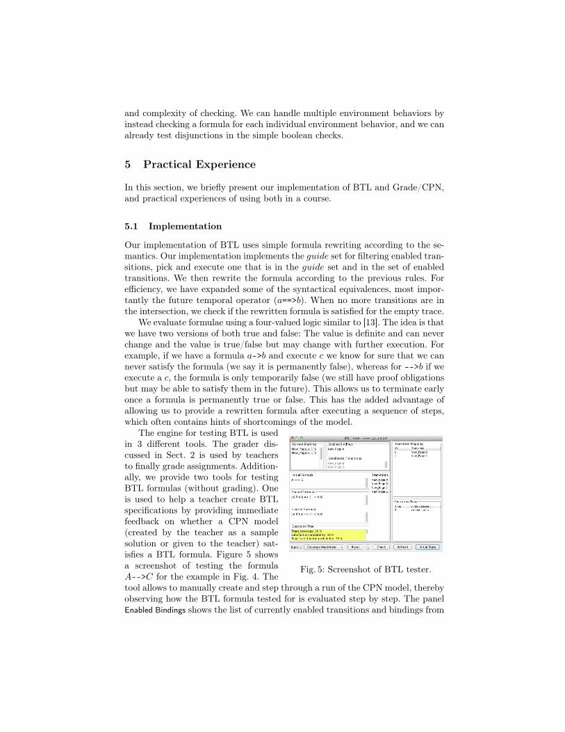
Fig. 5: Screenshot of BTL tester.

The engine for testing BTL is usedin 3 different tools. The grader dis-cussed in Sect. 2 is used by teachersto finally grade assignments. Addition-ally, we provide two tools for testingBTL formulas (without grading). Oneis used to help a teacher create BTLspecifications by providing immediatefeedback on whether a CPN model(created by the teacher as a samplesolution or given to the teacher) sat-isfies a BTL formula. Figure 5 showsa screenshot of testing the formulaA-->C for the example in Fig. 4. Thetool allows to manually create and step through a run of the CPN model, therebyobserving how the BTL formula tested for is evaluated step by step. The panelEnabled Bindings shows the list of currently enabled transitions and bindings from

which the user can pick one. Disallowed Transitions shows transitions not allowedby the guard function. The panel Current Marking shows the current marking inthe run. The panel Current Formula contains the remaining formula that has to beevaluated, whenever a step in the CPN model makes a subformula true or false,the formula in that panel is rewritten according to the BTL semantics of Sect. 3.The panel Execution Trace shows the steps of the run executed so far, includingtiming information which is valuable for assessing whether time-related guardsin the model match time-related conditions in the BTL formula. The tool alsoreports estimates of the coverage, probability the formula holds, and the proba-bility of a random trace satisfying the formula in the Decision Tree panel.

A simplified version of this tool allows students to check that their modelsconform to the formulas. Here, the tool is pre-packaged with a set of BTL for-mulas that the model must satisfy. The students loads their models and the toolautomatically tests validity of each formula on the model. In case one formulais not satisfied by the model, the student can manually single-step through themodel and watch the formula progress in an interface similar to Fig. 5, aiding infinding and fixing obvious errors before handing in.

5.2 Case Study: Business Information Systems

In this section, we present first experiences we made with Grade/CPN in sup-porting the evaluation of a CPN assignment in the course Business InformationSystems at Eindhoven University of Technology. In this assignment, studentswere given the base model in Fig. 1 and they had to model the delivery systemaccording to a textual specification. Each of the 94 students had to work on fivetasks; for each task, they had to submit one model. We received in total 258models from 66 students. Table 1 summarizes some statistics. We continue bydescribing the assessment in more detail and then report on the experiences had.Assessment. For each of the five tasks, the assessment consisted of two steps.In the first step, we applied Grade/CPN by calling it with a student model, thebase model, and a configuration file (see Listing 2). Here, we were interestedwhether the interface and declaration of the base model have been preserved,whether there is a suspicion of fraud, and whether, depending on the task, sixup to fourteen scenarios can be replayed on the model (only two are shownin the Listing). The scenarios were part of the specification of the assignment,and we specified them using BTL. As BTL refers to the interface, it is cru-cial that students have not changed it. The runtime of the tool was about tenminutes for all students in the case of Task 1 and 2 and about ten minutes

Table 1: Results of supporting the evaluation of 258 CPN models

Task hand-ins incorrect grader full points full pointsmodels incorrect by grader

1 66 8 0 58 582 64 8 0 56 563 56 49 7 2 64 41 32 4 6 65 31 20 2 0 0

for each student model in the case of Tasks 3–5. The reason for the differentruntime of Grade/CPN is that Tasks 1 and 2 are simple CPNs with few tests,whereas the remaining tasks performed more thorough tests on more advancedmodels, including performance analysis, thereby causing a higher analysis effort.Grade/CPN detected two fraud attempts, though they turned out to be causedby students handing in a subsequent assignment using the same base model. Ina subsequent run of the course, we caught two students cheating, even thoughthey had tried to conceal that by changing the layout. This attempt would beunlikely to get caught manually, but after singling out the models, we manuallyinspected them and saw they were clearly the same despite the obfuscation.

In the second step of the assessment, we manually checked each of the gen-erated reports. On average, this took less than five minutes for each report inthe case of Task 1 and 2 and about ten minutes in the case of Tasks 3–5. Basedon the feedback provided by Grade/CPN, it was easy to check whether a modelwas actually correct or not, in particular for the untimed CPN models. Basically,the violation of a certain scenario simplified the detection of the cause for thisviolation drastically. In most cases, we did not even have to look at the coun-terexample provided by our tool. For Tasks 1 and 2, we had to simulate onlyfive out of 130 student models manually to determine the cause of an error. Asimilar number of models had to be simulated manually for each of the Tasks3–5. In those cases, the effort spent on finding the cause of an error was oftenhigher because of the complexity of the models.

The tool automatically detected several subtle errors, such as wrong guardsand minor changes to the environment, without having the need to manuallyopen the respective model; it is highly unlikely we would have caught all ofthese completely manually. We even found subtle errors in our own solutions,yielding better results.Experiences and Evaluation. Based on experience from previous years, theuse of Grade/CPN reduced the amount of time for grading the assignment by afactor of at least two to three. This is factoring in that we used Grade/CPN forthe first time and had to both define and understand the defined logic BTL, andalso did not place complete confidence in the reported results which probablyincreased the manual labor as well. Table 1 confirms this observation: For eachtask, it shows the number of student models received (Col. 2), the number ofincorrect models (Col. 3), how many times Grade/CPN gave incorrect results(Col. 4), the number of student models that were graded to be correct accordingto the tool (Col. 5), and the number student models that were graded to becorrect after manually checking them (Col. 6). In fact, whenever the graderassigned full points to a model, then the model was correct. As a result, checkingthose models manually took almost no time. Given the high number of models forTasks 1 and 2, we saved a lot of time here. Column 4 shows that only few modelswere graded incorrectly. In most cases, the cause was a misinterpretation of thespecification on the part of the students where we decided that the studentsshould not be punished. Note that we do not show incorrect results of the toolcaused by problems specifying a scenario in BTL.

The second column shows that the number of students participating at theassignment decreased from 66 for Task 1 to 31 for Task 5. Moreover, the averagenumber of incorrect student solutions increased from 8/66=12% for Task 1 to20/31=65% for Task 5. The tasks became more difficult; whereas the first twotasks dealt with untimed CPN models and simple functionality, the remainingthree tasks were much more involved. However, for the last two tasks we providedstudents with a student version of Grade/CPN. The idea was to provide themwith a BTL specification that covers the basic functionality of their model. Thefinal BTL specification used by us to grade their assignment contained additionalscenarios. We experienced that providing students with Grade/CPN helped themto come up with better models. Whereas only 32/56 = 57% of the students gotat least half of the points for the third assignment (56−49 = 7 correct solutions),this number increased to 28/41 = 68% (11 correct) for Task 4 and 20/31 = 64%(11 correct) for Task 5 even though these were much more involved than theprevious tasks. Moreover, we observed that the overall quality of the modelsincreased drastically.

Grading models is a rather monotonous work. Therefore, it is easily possiblethat one oversees an error or forgets to check some scenario. Using Grade/CPN,this is now impossible and, therefore, we think that we can provide studentswith a fairer (in the sense of more equal) grading on the one hand and betterfeedback on the other hand.Coverage Criteria and Confidence. We also compared the quality of thetest result under the 3 different testing strategies (random exploration, increasingcoverage of the guided tree, increasing transition coverage) discussed in Sect. 4.We observed that random yields the least confidence in the validity of the for-mula. Increasing tree coverage raises coverage by factor 4 (compared to random)and increasing transition coverage raises coverage by factor 200 (compared torandom). Likewise, increasing the number of runs tested for also raises covarage.

6 Conclusion and Future Work

We have presented Grade/CPN, a tool to semi-automatically grade CPN mod-els. Using Access/CPN, we can support any model created using CPN Tools.The plug-in architecture makes the tool easily extendible: to do so, one mustjust implement the interface in Listing 1 (ll. 1–5). The pluggable configurationwith a very simple base format makes configuration simple. Configuration com-prises selecting which plug-ins to use, which weight to assign them, and whichparameters to instantiate them. Each plug-in only needs to consider its own op-tions as the overall configuration format is handled by Grade/CPN. Reportingis handled by making all plug-ins return simple messages optionally annotatedwith more detailed reasoning (Listing 1 ll. 13–15). The information is automat-ically gathered by Grade/CPN and presented both as an overview in the userinterface and as a detailed report. We have presented both simple plug-ins anda very powerful one implementing guided checking of Britney Temporal Logic(BTL). BTL allows us to guide the simulation toward desired scenarios and to

check that the environment contracts are adhered to. All plug-ins provide cat-egorized information explaining the score and highlighting any changes madeto the model, so teachers processing the reports only have to focus on thingsthat cannot be automatically checked. We have designed and implemented aninfrastructure for detecting fraud. We have reported on our experience with theBusiness Information Systems course where Grade/CPN was used to grade 258assignments from 94 students. Using Grade/CPN instead of a completely man-ual approach reduced the manual labor by a factor of two to three. Grade/CPNis being employed again in the same course and results show that the quality ofstudent models has significantly increased after giving them access to the studenttester.

The idea of (semi-)automatically grading assignments is not new and closelyrelated to testing. A known testing framework is JUnit [14], which also runs a setof tests and reports the result. The advantage of our tool over JUnit is that JUnitrequires programming to get started, whereas we use simple configuration files.From the testing world we also find the tool Jenkins (previously Hudson) [15],which runs tests on a central server and provides near-instantaneous feedback.The main disadvantage of Jenkins in our view is also complexity; while it doesnot (necessarily) require programming, setup does require complex XML con-figuration, and extension either requires huge effort or makes it difficult to getconsolidated reports. There are many tools for automatically grading program-ming assignments [16], for example, the tool peach3 [17], which more focuses onmanaging hand-ins, but can also run automatic tests. In contrast, we focus onthe tests and CPN models directly and assume that models already exist. Ourtesting approach is similar to runtime LTL [10, 13], but our logic also supportsguiding. This is similar to hot/cold events in Live-Sequence Charts [18], but oursections are more urgent in that a guide is not only preferred, it is an immediatefailure if it is not possible to follow it, making BTL computationally easier tocheck.

It is very interesting to increase the efficiency of the coverage heuristics forBTL, including expression abstraction, e.g., using a Counter-Example GuidedAbstraction Refinement (CEGAR) [19] or similar approach. It is also interestingto employ more static analysis to get even better coverage. Experience says,though, that students often fail to account for particular cases, making it veryeasy to detect errors in those cases. It would also be interesting to investigatesimpler languages. For example, it may be interesting for a teacher simply to seeif a given transition is enabled. This is easily expressible in BTL but difficult tocheck, and employing techniques from directed model-checking [20] may provebeneficial to try more intelligent guiding towards errors. We would also like toextend Grade/CPN with ability to provide simple simulation-based checks ofstandard safety and liveness properties. We also want to add support for loadingmodels in the PNML standard [21] format to be able to also check models createdusing other tools.

Acknowledgements. The authors thank Boudewijn van Dongen for fruitful dis-cussions about the requirements for an automatic grader.

References

1. Jensen, K., Kristensen, L.M.: Coloured Petri Nets – Modelling and Validation ofConcurrent Systems. Springer (2009)

2. van der Aalst, W.M.P., Stahl, C.: Modeling Business Processes – A Petri Net-Oriented Approach. MIT Press (2011)

3. Online: CPN Tools webpage. cpntools.org4. Westergaard, M., Kristensen, L.M.: The Access/CPN Framework: A Tool for In-

teracting With the CPN Tools Simulator. In: Proc. of ATPN. Volume 5606 ofLNCS., Springer (2009) 313–322

5. Westergaard, M., Fahland, D., Stahl, C.: Grade/CPN: Semi-automatic Supportfor Teaching Petri Nets by Checking Many Petri Nets Against One Specification.In: Proc. of PNSE. Volume 851 of CEUR Workshop Proceedings., CEUR-WS.org(2012) 32–46

6. Westergaard, M., Evangelista, S., Kristensen, L.M.: ASAP: An Extensible Platformfor State Space Analysis. In: Proc. of ATPN. Volume 5606 of LNCS., Springer(2009)

7. Pnueli, A.: The Temporal Logic of Programs. In: Proc. of SFCS ’77, IEEE Comp.Soc. (1977) 46–57

8. Kripke, S.: A semantical analysis of modal logic: I. Normal modal propositionalcalculi. Zeitschrift fur Mathematische Logic und Grundlagen der Mathematik 9(1963) 67–96

9. Plotkin, G.: A Structural Approach to Operational Semantics. DAIMI-FN 19,Department of Computer Science, University of Aarhus (1981)

10. Giannakopoulou, D., Havelund, K.: Automata-Based Verification of TemporalProperties on Running Programs. In: Proc. ASE, IEEE Computer Society (2001)412–416

11. Utting, M., Legeard, B.: Practical Model-Based Testing: A Tools Approach. Mor-gan Kaufmann Publishers (2006)

12. Weißleder, S.: Simulated satisfaction of coverage criteria on uml state machines.In: ICST 2012. (2010) 117–126

13. Bauer, A., Leucker, M., Schallhart, C.: Comparing LTL Semantics for RuntimeVerification. Logic and Computation 20(3) (2010) 651–674

14. Online: JUnit webpage. junit.org15. Online: Jenkins Continuous Integration webpage. jenkins-ci.org16. Ihantola, P., Ahoniemi, T., Karavirta, V., Seppälä, O.: Review of Recent Systems

for Automatic Assessment of Programming Assignments. In: Proc. InternationalConference on Computing Education Research, ACM (2010) 86–93

17. Verhoeff, T.: Programming Task Packages: Peach Exchange Format. Olympiadsin Informnatics 2 (2008) 192–207

18. Damm, W., Harel, D.: LSCs: Breathing Life into Message Sequence Charts. Form.Methods Syst. Des. 19(1) (2001) 45–80

19. Clarke, E., Grumberg, O., Jha, S., Lu, Y., Veith, H.: Counterexample-GuidedAbstraction Refinement for Symbolic Model Checking. J. ACM 50 (2003) 752–794

20. Edelkamp, S., Lafuente, A., Leue, S.: Directed Explicit Model Checking with HFS-SPIN. In: Proc. of SPIN. Volume 2057 of LNCS., Springer (2001) 57–79

21. ISO/IEC: Software and system engineering – High-level Petri nets – Part 2: Trans-fer format. ISO/IEC 15909-2:2011