graceful labeling of graphs · gracefulness of some graph classes as well as some general results...
TRANSCRIPT

GRACEFUL LABELING OF GRAPHS
Rodrigo Ming Zhou
Dissertação de Mestrado apresentada aoPrograma de Pós-graduação em Engenhariade Sistemas e Computação, COPPE, daUniversidade Federal do Rio de Janeiro, comoparte dos requisitos necessários à obtenção dotítulo de Mestre em Engenharia de Sistemas eComputação.
Orientadores: Celina Miraglia Herrera deFigueiredoVinícius Gusmão Pereira de Sá
Rio de JaneiroDezembro de 2016

GRACEFUL LABELING OF GRAPHS
Rodrigo Ming Zhou
DISSERTAÇÃO SUBMETIDA AO CORPO DOCENTE DO INSTITUTOALBERTO LUIZ COIMBRA DE PÓS-GRADUAÇÃO E PESQUISA DEENGENHARIA (COPPE) DA UNIVERSIDADE FEDERAL DO RIO DEJANEIRO COMO PARTE DOS REQUISITOS NECESSÁRIOS PARA AOBTENÇÃO DO GRAU DE MESTRE EM CIÊNCIAS EM ENGENHARIA DESISTEMAS E COMPUTAÇÃO.
Examinada por:
Prof. Celina Miraglia Herrera de Figueiredo, D.Sc.
Prof. Vinícius Gusmão Pereira de Sá, D.Sc.
Prof. Rosiane de Freitas Rodrigues, D.Sc.
Prof. Raphael Carlos Santos Machado, D.Sc.
RIO DE JANEIRO, RJ – BRASILDEZEMBRO DE 2016

Zhou, Rodrigo MingGraceful Labeling of Graphs/Rodrigo Ming Zhou. – Rio
de Janeiro: UFRJ/COPPE, 2016.IX, 40 p.: il.; 29, 7cm.Orientadores: Celina Miraglia Herrera de Figueiredo
Vinícius Gusmão Pereira de SáDissertação (mestrado) – UFRJ/COPPE/Programa de
Engenharia de Sistemas e Computação, 2016.Bibliography: p. 38 – 40.1. graceful labeling. 2. computational proofs.
3. graphs. I. de Figueiredo, Celina Miraglia Herreraet al. II. Universidade Federal do Rio de Janeiro, COPPE,Programa de Engenharia de Sistemas e Computação. III.Título.
iii

Resumo da Dissertação apresentada à COPPE/UFRJ como parte dos requisitosnecessários para a obtenção do grau de Mestre em Ciências (M.Sc.)
GRACEFUL LABELING OF GRAPHS
Rodrigo Ming Zhou
Dezembro/2016
Orientadores: Celina Miraglia Herrera de FigueiredoVinícius Gusmão Pereira de Sá
Programa: Engenharia de Sistemas e Computação
Em 1966, A. Rosa propôs uma nova coloração de grafos chamada coloração-βem que os vértices são coloridos com números distintos entre 0 a m, onde m é onúmero de arestas, tal que cada aresta é rotulada com o módulo da diferença dascores dos seus vértices extremos e cada um é único no grafo. Alguns anos depois,S. W. Golomb renomeou essa coloração de coloração graciosa, como é conhecidahoje em dia.
Esta definição permitiu que Rosa mostrasse que se toda árvore admitisse umacoloração graciosa, então uma conjectura de G. Ringel seria verdadeira. A partirdisso, foi conjecturado que toda árvore fosse graciosa, a Conjectura das ÁrvoresGraciosas.
Este trabalho apresenta alguns dos principais resultados em coloração graciosade grafos e também apresenta esforços computacionais na direção da Conjecturadas Árvores Graciosas. Inspirado por isso, nós também tomamos a abordagemcomputacional para estender a graciosidade de grafos cones generalizados.
iv

Abstract of Dissertation presented to COPPE/UFRJ as a partial fulfillment of therequirements for the degree of Master of Science (M.Sc.)
GRACEFUL LABELING OF GRAPHS
Rodrigo Ming Zhou
December/2016
Advisors: Celina Miraglia Herrera de FigueiredoVinícius Gusmão Pereira de Sá
Department: Systems Engineering and Computer Science
In 1966, A. Rosa introduced a new graph labeling called β-labeling in which thevertices are labeled with distinct numbers chosen from 0 tom, wherem is the numberof edges, such that each edge is labeled with the absolute difference of the labelsof its end vertices and it is unique in the graph. A few years later, S. W. Golombrenamed β-labeling as graceful labeling as it is known today.
This definition allowed Rosa to show that if every tree admits a graceful labeling,then a conjecture from G. Ringel would hold, from which it was conjectured thatevery tree is graceful, the Graceful Tree Conjecture.
This work presents some of the main results on graceful labeling of graphs andalso presents computational efforts in the direction of the Graceful Tree Conjecture.Inspired by that, we also took the computational approach to extend the gracefulnessof generalized cone graphs.
v

Contents
List of Figures vii
List of Tables viii
List of Algorithms ix
1 Introduction 11.1 Definitions . . . . . . . . . . . . . . . . . . . . . . . . . . . . . . . . . 2
2 Graceful Labeling 42.1 General results . . . . . . . . . . . . . . . . . . . . . . . . . . . . . . 62.2 Gracefulness of graph classes . . . . . . . . . . . . . . . . . . . . . . . 9
3 Trees 133.1 Trees with limited diameter . . . . . . . . . . . . . . . . . . . . . . . 133.2 All trees up to 35 vertices are graceful . . . . . . . . . . . . . . . . . 163.3 Relaxed versions . . . . . . . . . . . . . . . . . . . . . . . . . . . . . 19
4 Generalized Cone Graphs 254.1 Graceful cones . . . . . . . . . . . . . . . . . . . . . . . . . . . . . . . 264.2 Computational results . . . . . . . . . . . . . . . . . . . . . . . . . . 31
5 Conclusion 36
Bibliography 38
vi

List of Figures
2.1 Graceful labeling of P3 and K1,3. . . . . . . . . . . . . . . . . . . . . 42.2 Graceful labeling of K3 and K4. . . . . . . . . . . . . . . . . . . . . . 52.3 Constructing a graceful graph from C5. . . . . . . . . . . . . . . . . . 82.4 Graceful labeling of caterpillar tree. . . . . . . . . . . . . . . . . . . . 112.5 Graceful labelings of Kp,q, K1,p,q, K2,p,q, and K1,1,p,q. . . . . . . . . . 12
3.1 Transfer of subtrees from u to v. . . . . . . . . . . . . . . . . . . . . . 153.2 Transfer of leaves from m to 0 (m→ 0 transfer). . . . . . . . . . . . . 153.3 Labeling of Theorem 3.6 at level i even. . . . . . . . . . . . . . . . . . 203.4 Splitting the tree at the vertex v. . . . . . . . . . . . . . . . . . . . . 22
4.1 Graceful labeling of C4 + I2. . . . . . . . . . . . . . . . . . . . . . . . 26
vii

List of Tables
4.1 Gracefulness of Cp + Iq (updated as of 2014). . . . . . . . . . . . . . . 304.2 Gracefulness of Cp + Iq (shaded entries are new results). . . . . . . . 35
viii

List of Algorithms
3.1 Backtracking search . . . . . . . . . . . . . . . . . . . . . . . . . . . . 183.2 Local search using metaheuristics . . . . . . . . . . . . . . . . . . . . . 19
4.1 Backtracking search for generalized cone graphs . . . . . . . . . . . . . 32
ix

Chapter 1
Introduction
Suppose we want to decompose a complete graph G into trees, all of them iso-morphic between themselves. In other words, we want to partition the edges of Gsuch that the subgraph induced by each set of edges of the partition is isomorphicto a given tree T . Ringel [20] conjectured that, for any tree T with n vertices, thecomplete graph K2n−1 can be decomposed into 2n− 1 trees isomorphic to T .
Rosa [21] introduced graceful labeling in 1966, and, back then, he called it β-labeling. The term “graceful” was introduced by Golomb [12] in 1972. Rosa showedthat if every tree is graceful, then Ringel’s conjecture holds. Since then, researchershave been trying to prove Ringel’s conjecture through the Graceful Tree Conjecture,which claims that every tree is graceful.
However, graceful graphs gained their own merit of study over the years. DavidS. Johnson, in his NP-completeness column of 1983 [16], includes the decision prob-lem of graceful labeling as the “Open Problem of the Month”. Moreover, there isthe International Workshop on Graph Labeling in which graceful labeling is one ofthe main themes, and a complete survey on the subject from Gallian [11] that isconstantly updated.
In Section 1.1, we give the definitions used throughout the text. In Chapter 2,we present the formal definition of graceful labeling of a graph and present thegracefulness of some graph classes as well as some general results about gracefullabeling of graphs. In Chapter 3, we focus on results towards the Graceful TreeConjecture, presenting different approaches to tackle the conjecture. Finally, inChapter 4 we change our focus to generalized cone graphs, a graph class definedby the join of two graphs. We review known theoretical results and propose newcomputational results which establish the gracefulness of families of generalized conegraphs and suggest a conjecture regarding the non-graceful ones.
1

1.1 Definitions
In this section, we give most of the definitions and notation of graph theory usedin this text. For any missing definition, see Bondy and Murty [7].
A graph G is an ordered pair (V,E) where V is a set of elements called verticesand E is a set of unordered pairs of distinct vertices from V called edges. We sayan edge e connects two vertices u and v, denoting as e = uv, and we say u and v areadjacent if they are connected by an edge. The set of adjacent vertices of a vertexu is denoted as N(u), and it is also called the set of neighbors of u. The degree ofa vertex u is d(u) = |N(u)|, the number of neighbors of u.
For a given graph G, when the vertex set and the edge set are not given explicitly,we refer to them as V (G) and E(G), and we use the letters n and m as the numberof vertices and edges, respectively.
A subgraph H of G is a graph such that V (H) ⊆ V (G) and E(H) ⊆ E(G).For a graph G = (V,E) and a subset W ⊆ V , the subgraph of G induced by W ,denoted as G[W ], is the graph H = (W,F ) such that, for all u, v ∈ W , if uv ∈ E,then uv ∈ F . We say H is an induced subgraph of G. Equivalently, we can definesubgraphs and induced subgraphs in terms of deletion of vertices and edges: H is aninduced subgraph of G if it is obtained by deletion of vertices, and H is a subgraphof G if it is obtained by deletion of vertices and edges.
A walk in a graph is a finite sequence of vertices W = (v0, v1, . . . , vk) such thatvivi+1 is an edge of the graph. If the walk W does not go through an edge twice, wesay W is a trail, and if it does not go through a vertex twice, we say W is a path. Apath starting in u and ending in v is called a uv-path.
The length of a path is the number of its edges and the distance between twovertices u and v is the length of the shortest path between them and denoted asdist(u, v). If there is no path between u and v, then dist(u, v) =∞.
A walk is said to be closed if the first and the last vertices are the same. A cycleis a closed trail in which all vertices, but the last, are distinct.
An Eulerian trail (or Eulerian path) of a graph is a trail that traverses each edgeof the graph exactly once. Similarly, an Eulerian tour (or Eulerian cycle) is a cyclethat traverses each edge exactly once. A graph is Eulerian if it admits an Euleriancycle.
A graph G is said to be connected if every pair of vertices is connected by apath. If there is exactly one path connecting each pair of vertices, we say G is atree. Equivalently, a tree is a connected graph with n− 1 edges (see [7]).
A path graph Pn is a connected graph on n vertices such that each vertex hasdegree at most 2. A cycle graph Cn is a connected graph on n vertices such thatevery vertex has degree 2.
2

A complete graph Kn is a graph with n vertices such that every vertex is adjacentto all the others. On the other hand, an independent set is a set of vertices of agraph in which no two vertices are adjacent. We denote In for an independent setwith n vertices.
A bipartite graph G = (V,E) is a graph such that there exists a partitionP = (A,B) of V such that every edge of G connects a vertex in A to one in B.Equivalently, G is said to be bipartite if A and B are independent sets. The bipar-tite graph is also denoted as G = (A,B,E).
The join of two graphs G1 = (V1, E1) and G2 = (V2, E2) with disjoint vertex setsis the graph G = (V,E) such that V = V1 ∪ V2 and E = E1 ∪E2 ∪ {uv : u ∈ V1, v ∈V2}, that is, G is obtained by connecting every vertex of G1 to every vertex of G2.
Finally, for a given graph G = (V,E), a vertex labeling (or vertex coloring) of Gis a function f : V → N, and an edge labeling (or edge coloring) of G is a functiong : E → N. Intuitively, we are assigning labels (colors) to vertices and/or edges ofthe graph. Throughout this text, we have the codomains as a finite subset of N, andwe denote [a, b] = {a, a+ 1, . . . , b}.
Many problems of graph theory consist in finding a vertex or an edge labelingfor a graph satisfying certain properties. For example, a proper vertex coloring isa vertex coloring such that adjacent vertices have different colors, and a very wellknown problem is to find for a given graph G the minimum k such that there existsa proper vertex coloring f of G with |Im(f)| = k. In our case, we are interested ingraceful labeling.
3

Chapter 2
Graceful Labeling
A graceful labeling of a graph G is a vertex labeling f : V → [0,m] such that f isinjective and the edge labeling fγ : E → [1,m] defined by fγ(uv) = |f(u)− f(v)| isalso injective. If a graph G admits a graceful labeling, we say G is a graceful graph.
Although it has been studied for 50 years, not many general results are knownabout graceful labeling. Most of the results are about asserting the gracefulnessof a graph class since it suffices to show a graceful labeling for each graph in theclass. On the other hand, results on non-gracefulness of a graph rely basically on anecessary condition only valid for Eulerian graphs (see Theorem 2.4) or on trying tolabel the graph gracefully until reaching a contradiction, which is not very effectivein most of the cases.
0 1 23
123
12
3
1
3
0
2
Figure 2.1: Graceful labeling of P3 and K1,3.
To gain some intuition on how to label a graph gracefully, let us show how tolabel a path graph. So, take a path graph Pn and let V (Pn) = {u0, u1, . . . , un−1}be the set of vertices such that uk−1uk ∈ E(Pn) for 0 < k < n. Since Pn hasm = n− 1 edges, we must label the vertices with numbers from 0 to n− 1 so thatevery number in [1, n− 1] appears as an edge label. We start with edge label n− 1
since there is only one way to get an absolute difference equal to n − 1, which ishaving a vertex with label 0 adjacent to a vertex with label n− 1. Thus, let us trylabeling u0 with 0 and u1 with n − 1. Next, let us try to get an edge label withvalue n− 2. There are only two possible ways to get n− 2 as an absolute difference:n − 2 = |(n − 2) − 0| = |(n − 1) − 1|. Since u0 has no more unlabeled adjacent
4

vertices, we can only get the edge label n− 2 by labeling u2 with 1. Going on withthis strategy, our resulting labeling will be as follows:
f(uk) =
k2
if k is even
n− k+12
if k is odd
Now, to show that f is indeed a graceful labeling of Pn, it suffices to show that theedge label 1 appears, which is expected to appear on the last edge un−2un−1. If nis even, then f(un−1) = n
2and f(un−2) = n−2
2. Hence, fγ(un−1un−2) = n
2− n−2
2= 1.
If n is odd, an analogous argument establishes the edge label 1. Therefore, thefollowing proposition holds.
Proposition 2.1. The path graph Pn is graceful for all n ≥ 1.
For a second example, we try to find a graceful labeling for the complete graphKn. Since K1 and K2 are also path graphs, they are graceful. For K3 and K4,Figure 2.2 presents a graceful labeling for each one.
0
1
3
1 2
3 0
1
2
3
4
5
6
1
4
6
Figure 2.2: Graceful labeling of K3 and K4.
Before analysing the general case, let us first introduce a property of gracefullabelings. Given a graph with a graceful labeling, if we swap every vertex label kwith m− k, the resulting labeling is also graceful since the edge labels will not havechanged: the end vertices of an edge with labels a and b become m− a and m− b,and |a− b| = |(m− a)− (m− b)|. This is called the complementarity property.
Now, for Kn with n > 4, as before, we must have a vertex with label 0 adjacentto a vertex labeled m to get the edge label m. But, in this case, every vertexis adjacent to every other vertex. Thus, we can label any vertex with 0 and anyother one with m without loss of generality. To get the edge label m − 1, we havetwo options: m − 1 = |(m − 1) − 0| = |m − 1|. However, the complementarityproperty allows us to choose either one without loss of generality. Choosing to labela vertex with 1, we get edge labels 1 and m − 1. Now we need to get the edgelabel m − 2 = |(m − 2) − 0| = |(m − 1) − 1| = |m − 2|. We can not label a vertexwith m − 1 or 2 because it would create a duplicate edge label. Hence, our onlyoption is to label a vertex with m − 2, obtaining edge labels 2, m − 3 and m − 2.
5

Since m − 3 has already appeared on an edge, the next edge label we must obtainis m− 4 = |(m− 4)− 0| = |(m− 3)− 1| = |(m− 2)− 2| = |(m− 1)− 3| = |m− 4|.Again, we only have one option without creating duplicate edge labels, which is tolabel a vertex with 4, obtaining edge labels 3, 4, m− 6 and m− 4. At this point, wehave labeled five vertices. However, for K5, we would have m− 6 = 4 as a duplicateedge label. For n ≥ 6, the next edge label to get is m− 5. But, all the five possibleways to get m− 5 lead to a duplicate edge label. Therefore, there is no way to getlabel m− 5 on an edge and the following proposition holds.
Proposition 2.2. The complete graph Kn is graceful if, and only if, n ≤ 4.
Given the initial intuition on how to gracefully label a graph, Section 2.1 presentssome general results on graceful graphs and Section 2.2 shows the gracefulness ofsome graph classes.
2.1 General results
We start by showing a couple of results concerning necessary conditions to theexistence of a graceful labeling of a graph. The first one is a straightforward conditiongiven by Golomb [12].
Proposition 2.3. If G = (V,E) is graceful, then there exists a partition P = (A,B)
of V such that the number of edges with one end in A and the other in B is dm2e.
Proof. Let G = (V,E) be a graph with a graceful labeling f and consider thepartition P = (A,B) of V such that A = {u ∈ V : f(u) ≡ 0 (mod 2)}. Sincethere are dm
2e odd values between 1 and m, and an odd difference is only possible
by subtracting an even value from an odd one, the number of edges connecting twovertices with different parities must be exactly dm
2e.
Although Proposition 2.3 gives a necessary condition to the existence of a gracefullabeling for a graph, it has no practical use since it would be necessary to check allthe 2n−1 possible partitions of V to decide if a graph can admit a graceful labeling.
A more useful necessary condition was given by Rosa [21], but it only applies toEulerian graphs. It is known as the parity condition.
Theorem 2.4. Let G be an Eulerian graph. If m ≡ 1, 2 (mod 4), then G is notgraceful.
Proof. Suppose G = (V,E) is a graceful Eulerian graph. Let f : V → [0,m] be agraceful labeling of G and C = (u0, u1, . . . , um−1, um = u0) be an Eulerian cycle of
6

G. Taking the sum of the edge labels of C modulo 2, we have:
m∑i=1
fγ(ui−1ui) =m∑i=1
|f(ui−1)− f(ui)|
≡m∑i=1
f(ui−1)− f(ui) ≡ 0 (mod 2)
(2.1)
And, since C is an Eulerian cycle, i.e., the cycle C goes through each edge exactlyonce, and f is a graceful labeling of G, we have:
∑e∈E
fγ(e) =m∑k=1
k =m(m+ 1)
2
(2.1)≡ 0 (mod 2) (2.2)
Thus, we must have m ≡ 0, 3 (mod 4) in order to satisfy equation (2.2).
The parity condition, unlike Proposition 2.3, provides a simple way to test if anEulerian graph can be graceful or not. And an interesting question arises: is there agraph class for which the parity condition is also a sufficient condition? As we willsee, the parity condition does characterize at least one graph class.
In graph theory, it is natural to think of substructures that make a graph notsatisfy a certain property, in this case being graceful. Such substructures can besubgraphs, induced subgraphs, or others, and they are called forbidden substructuresfor the graph class. Thus, one might think of finding forbidden substructures forthe class of graceful graphs. However, Arumugam and Bagga [3] proved that everygraph is an induced subgraph of a graceful graph.
Theorem 2.5. Every graph is an induced subgraph of a graceful graph.
Proof. Given a graph G = (V,E), let us construct a graph H from G such that H isgraceful andG is an induced subgraph ofH. Consider a vertex labeling f : V → [0, k]
injective for some k ≥ m such that the edge labeling fγ : E → N is also injective,and there exist u, v ∈ V with f(u) = 0 and f(v) = k. Let {x1, x2, . . . , xr} be theset of missing edge labels. Without loss of generality, x1, x2, . . . , xs are not vertexlabels and xs+1, . . . , xr are vertex labels. For each xi, 1 ≤ i ≤ s, add a vertex wiwith label xi and add an edge connecting wi to u so that fγ(uwi) = xi. For eachxi, s + 1 ≤ i ≤ r, add a vertex wi with label k + xi and connect wi to u and v
so that fγ(uwi) = k + xi and fγ(vwi) = xi. Note that the last step might haveintroduced new missing edge labels by creating vertex labels with values greaterthan k. However, these new missing edge labels are not vertex labels. So, for eachnew missing edge label y, add a new vertex zy with label y and connect zy to u sothat fγ(uzy) = y. The resulting graph H is graceful and it contains G as an inducedsubgraph.
7

0
4
5
2
7
13
5
7
4
0
4
5
2
7
13
5
7
4
69
2 96
0
4
5
2
7
13
5
7
4
69
2 96
88
Figure 2.3: Constructing a graceful graph from C5.
Theorem 2.5 says that a graph G being non-graceful does not matter for graphsfor which G is an induced subgraph. It also says that we can always construct agraceful graph from any graph.
So far, we have characterized the gracefulness of two families of graphs: the pathgraphs and the complete graphs. The first one is a family of graceful graphs andthe second one, for n ≥ 5, is a family of non-graceful graphs. We have also shownthat we can construct a graceful graph from any graph, graceful or not.
Next, we present an unpublished result of Erdős [12]. The following proof wasgiven by Graham and Sloane[13].
Theorem 2.6. Almost all graphs are not graceful.
Proof. We show that for a fixed number m, almost all graphs with n vertices andm edges are not graceful as n→∞.
First, note that there are(n(n−1)/2
m
)labeled graphs with n vertices and m edges.
So, the number of unlabeled graphs is at least 1n!
(n(n−1)/2
m
).
Let f be a vertex labeling on n vertices with distinct numbers from [0,m]. Thereare (m+1)!
(m−n+1)!≤ (m + 1)n such labelings. Let us count how many graphs there are
for which f is a graceful labeling. Let pi be the number of pairs of vertices {u, v}with |f(u) − f(v)| = i. Clearly,
∑mi=1 pi =
(n2
). If we construct a graph by taking
one edge from each class counted by pi, the resulting graph is graceful. Thus, thereare
∏mi=1 pi labeled graphs for which f is a graceful labeling. Since this product
is maximized when all pi’s are equal,∏m
i=1 pi ≤ (n(n−1)2m
)m. Therefore, there are atmost (m+1)n(n(n−1)
2m)m graceful labeled graphs, and this is also an upper bound for
the number of graceful unlabeled graphs. Finally, we show that the ratio
ρ =(m+ 1)n(n(n−1)
2m)m
1n!
(n(n−1)/2
m
)
8

goes to 0 as n→∞. Writing m = (12− µ)
(n2
)with µ ∈ (−1
2, 12), we have
ρ =(m+ 1)nn!
(12− µ)m
((n2
)m
) <(m+ 1)nn!
√8(n2
)(12− µ)(1
2+ µ)
(12− µ)m2(
n2)H2(1/2−µ)
where H2(x) = −x log2(x) − (1 − x) log2(1 − x) (cf. [18, p. 309]). Simplifying thedenominator,
ρ <(m+ 1)nn!
√8(n2
)(12− µ)(1
2+ µ)
2−(n2)(
12+µ) log2(
12+µ)
Taking the logarithm, it is easy to show that the right hand side of the inequalitygoes to −∞ as n→∞. Therefore, ρ→ 0 as n→∞.
We finish this section by giving another construction of graceful graphs given byAcharya [1].
The full augmentation of a graceful graph G = (V,E) is the addition of anisolated vertex to G for each vertex label not used. Formally, Gf = G ∪ Im−n+1 isthe full augmentation of G. Clearly, Gf is also graceful and, in particular, gracefultrees are already full augmented.
Theorem 2.7. If G is a graceful graph and Gf is its full augmentation, then Gf+Iq
is graceful for all q ≥ 1.
Proof. Let f : V (Gf )→ [0,m] be a graceful labeling of Gf and V (Iq) = {v0, v1, . . . ,vq−1}. Then, we can extend the labeling f to V (Iq) as follows: label vi with f(vi) =m+ (i+ 1)(m+ 1).
We have |E(Gf + Iq)| = m+ q(m+1) and, since we are extending f , we alreadyhave Im(f
∣∣V (Gf )
) = [0,m] and Im(fγ∣∣E(Gf )
) = [1,m]. By definition of f , everyvertex label is unique, and the set of labels on the edges incident with vi is exactly[m+i(m+1),m+(i+1)(m+1)]. Then, every label in [1,m+q(m+1)] appears onceon some edge. Therefore, the extension of f is a graceful labeling of Gf + Iq.
2.2 Gracefulness of graph classes
In this section, we present the gracefulness of some graph classes. Most of theresults asserting the gracefulness of a graph class are given by explicit gracefullabelings. For the non-gracefulness of a graph class, there are only a few tools forthat. Basically, we only have Proposition 2.3 and theorem 2.4. We can also proveby trying to label the graph and finding a contradiction. For instance, Rosa [21]showed Proposition 2.2 this way. Although the last method is not effective if done
9

by hand, if it is done computationally, it may result in something useful, as we willsee later in following chapters.
It was already shown that the path graph Pn is graceful and the complete graphKn is graceful if, and only if, n ≤ 4. Next, we present the gracefulness cycle graphs,which was characterized by Rosa [21].
Proposition 2.8. The cycle graph Cn is graceful if, and only if, n ≡ 0, 3 (mod 4).
Proof. Cycle graphs are Eulerian graphs. Therefore, by the parity condition, if n ≡1, 2 (mod 4), then Cn is not graceful. Otherwise, let us call V (Cn) = {u0, u1, . . . ,un−1} such that ukuk+1 ∈ E(Cn) for 0 ≤ k ≤ n− 1 and un = u0.
If n ≡ 0 (mod 4), then label the vertices according to the following formula:
f(ui) =
i2
if i = 0, 2, 4, . . . , n− 2
n− i−12
if i = 1, 3, 5, . . . , n2− 1
n− i−12− 1 if i = n
2+ 1, n
2+ 3, . . . , n− 1
If n ≡ 3 (mod 4), then label V (Cn) as follows:
f(ui) =
i2
if i = 0, 2, 4, . . . , n− 1
n− i−12
if i = 1, 3, 5, . . . , n+12− 1
n− i−12− 1 if i = n+1
2+ 1, n+1
2+ 3, . . . , n− 2
Note that the parity condition characterizes the gracefulness of cycle graphs.The wheel graph Wp is the join of a cycle graph Cp with a singleton graph, i.e.,
Wp = Cp +K1. Frucht [10] showed that all wheels are graceful.
Proposition 2.9. The wheel graph Wp is graceful for all p ≥ 3.
Proof. Let V (Wp) = {u0, u1, . . . , up−1, v} be the set of vertices where v is the vertexjoined with the cycle and consider the following two cases.
1. If p ≡ 0 (mod 2), then the following formula gives a graceful labeling:
f(v) = 0
f(ui) =
2p if i = 0
2 if i = p− 1
i if i = 1, 3, 5, . . . , p− 3
2p− i− 1 if i = 2, 4, 6, . . . , p− 2
10

2. If p ≡ 1 (mod 2), then the following formula gives a graceful labeling:
f(v) = 0
f(ui) =
2p if i = 0
2 if i = 1
p+ i if i = 2, 4, 6, . . . , p− 1
p+ 1− i if i = 3, 5, 7, . . . , p− 2
A caterpillar is a tree in which the removal of all leaves results in a path graph.It was proven by Rosa [21] that they are all graceful.
Proposition 2.10. All caterpillar trees are graceful.
Proof. Draw the caterpillar tree as a planar bipartite representation and label it asshown in Figure 2.4. It is easy to check that such drawing scheme is always possible.
Figure 2.4: Graceful labeling of caterpillar tree.
Note that a path graph Pn is also a caterpillar tree and the labeling schemegiven by Proposition 2.10, when applied to a path graph, yields the same labelingconstructed before.
The complete bipartite graph Kp,q is a bipartite graph G = (A,B,E) such that|A| = p, |B| = q, and if u ∈ A and v ∈ B, then uv ∈ E. In particular, the stargraph is the complete bipartite graph K1,q.
It was shown that for all positives values of p and q, the complete bipartite graphsare graceful [12, 21].
Proposition 2.11. The complete bipartite graph Kp,q is graceful for all p, q ≥ 1.
11

Proof. Let G = (A,B,E) be a bipartite graph with a = |A| and b = |B|. Assignthe vertices from A with numbers 0, 1, . . . , a − 1, and assign the vertices from B
with numbers a, 2a, . . . , ba.
We can generalize the concept of bipartite graph to multipartite graph and, in asimilar fashion, we have the complete multipartite graph. It was proven the followingproposition regarding the gracefulness of complete multipartite graphs [5].
Proposition 2.12. The complete multipartite graphs Kp,q, K1,p,q, K2,p,q, and K1,1,p,q
are graceful.
Proof. The graceful labelings are given in Figure 2.5.
Figure 2.5: Graceful labelings of Kp,q, K1,p,q, K2,p,q, and K1,1,p,q.
Furthermore, Beutner [5] conjectured that these graphs are the only completemultipartite graphs which are graceful, and showed computationally that it is validfor all complete multipartite graphs up to 23 vertices.
12

Chapter 3
Trees
The Graceful Tree Conjecture remains unsolved to these days and there havebeen a few different approaches researchers have been trying to prove the conjecture.In this section, we present results on the gracefulness of trees and the different waysin which the conjecture has been tackled.
Conjecture 3.1 (Graceful Tree Conjecture). Every tree is graceful.
As shown in Chapter 2, paths and caterpillars are graceful. A first approachwould be to extend the definition of caterpillars to new families of trees, i.e., look atthe class of trees in which the removal of all leaves results in a caterpillar tree—thelobsters—, and so on. However, even the lobster trees have not been characterizedyet. Bermond [4] conjectured in 1979 that all lobsters are graceful. This chapterpresents others approaches which have shown to be more interesting.
3.1 Trees with limited diameter
The diameter of a tree T is the maximum distance between two vertices, i.e.,diam(T ) = max{dist(u, v) : u, v ∈ V (T )}. Trees with small diameter have beenproved to be graceful. We already showed that trees with diameter 1 (only K2),diameter 2 (star graphs), and diameter 3 (a subclass of caterpillar trees) are gracefulsince they are all also caterpillar trees. For greater diameters, Zhao [28] proved in1989 that all trees with diameter 4 are graceful, Hrnčiar and Haviar [15] proved in2001 that all trees with diameter 5 are graceful, and Superdock [23, 24] proved morerecently that some subclasses of trees with diameter 6 are graceful.
We show in this section that all trees with diameter 4 are graceful. The proofpresented here was given by Hrnčiar and Haviar [15] since it is simpler than theoriginal proof of Zhao [28].
13

Lemma 3.1. Let T be a tree with a graceful labeling f and let u ∈ V (T ) the vertexwith f(u) = 0. If T ′ is the tree obtained from T by adding a new vertex v onlyadjacent to u, then T ′ is graceful.
Proof. If m is the number of edges of T , then the vertex labeling f ′ such thatf ′∣∣V (T )
= f and f ′(v) = m+ 1 is a graceful labeling of T ′.
Corollary 3.1.1. If w ∈ V (T ) has label m, then adding a new vertex only adjacentto w also results in a graceful tree.
Proof. Just consider the complementary graceful labeling of f .
Corollary 3.1.2. If u ∈ V (T ) has label 0 (or m) and H is a caterpillar tree, thenadding an edge between u and a vertex of H with maximum eccentricity also resultsin a graceful tree.
Proof. Apply iteratively Lemma 3.1 giving preference to adding leaves first wheneverit is possible. Also note that the corollary is valid for any graceful graph G as longas u ∈ V (G) has label 0 (or m).
Lemma 3.1 allows us to obtain new graceful graphs from smaller ones by addinga vertex. Then, it is reasonable to ask if this could be used to prove the GracefulTree Conjecture, i.e., somehow show that for any tree, there is a finite sequence ofgraceful trees starting from a single vertex such that each tree is the previous one inthe sequence plus a vertex, and the last tree of the sequence is the target tree itself.
One sufficient condition to the existence of such sequence is if every tree admitsa graceful labeling in which the label 0 can be assigned to any vertex. In the generalcontext, such graphs are called 0-rotatable graceful graphs. However, it is not truethat every tree is 0-rotatable graceful [26].
Let T be a tree and uv ∈ E(T ). We denote by Tu,v the subtree of T containing vafter the removal of the edge uv. Precisely, if S = {w ∈ V (T ) : v is on the uw-path},then Tu,v = T [S].
Lemma 3.2. Let T be a tree with a graceful labeling f and let u ∈ V (T ) be a vertexadjacent to u1 and u2. Consider T ′ = T − (V (Tu,u1) ∪ V (Tu,u2)) and let v ∈ V (T ′),v 6= u.
(a) If u1 6= u2 and f(u1) + f(u2) = f(u) + f(v), then the tree obtained bya disjoint union of T ′, Tu,u1 and Tu,u2, and connecting v to u1 and u2 isgraceful with the same graceful labeling f .
(b) If u1 = u2 and 2f(u1) = f(u) + f(v), then the tree obtained by a disjointunion of T ′ and Tu,u1, and connecting v to u1 is graceful with the samegraceful labeling f .
14

Proof. It suffices to show that the edge labels of uu1 and uu2 are the same as of vu1and vu2.
(a) |f(u1)− f(u)| = |f(u) + f(v)− f(u2)− f(u)| = |f(v)− f(u2)||f(u2)− f(u)| = |f(u) + f(v)− f(u1)− f(u)| = |f(v)− f(u1)|
(b) |f(u1)− f(u)| = |f(u)+f(v)2− f(u)| = |f(v)−f(u)
2|
|f(u1)− f(v)| = |f(u)+f(v)2− f(v)| = |f(u)−f(v)
2|
Figure 3.1: Transfer of subtrees from u to v.
This operation is called a transfer and we mostly do transfers of leaves from onevertex to another. For the remaining of this section, for a graceful tree, we no longerdistinguish the vertex label from the vertex itself since in a tree every number from[0, n− 1] must appear as a vertex label.
As an example, take the star graph K1,m. We can transfer some leaves, whichis connected to vertex 0, to the vertex m (see Figure 3.2). For an example, we cantransfer k and m − k from 0 to m since k + (m − k) = 0 +m. As said before, thesubtree being transferred is usually a leaf and we denote a sequence of transfers ofleaves adjacent to u to v as u→ v. Although the notation is not precise, the contextwill make clear how many and which leaves are being transferred.
(a) (b)
Figure 3.2: Transfer of leaves from m to 0 (m→ 0 transfer).
15

Proposition 3.3. All trees with diameter 4 are graceful.
Proof. Consider the following types of transfers.A u→ v transfer is of type 1 if the leaves being transferred are k, k+1, . . . , k+s.
This type of transfer can be realized if u + v = k + (k + s). We use this type oftransfer when we want to leave an odd number of vertices connected to u.
A u→ v transfer is of type 2 if the leaves being transferred are k, k+1, . . . , k+s
and l, l + 1, . . . , l + s with k + s < l. This type of transfer can be realized ifu + v = k + (l + s). We use this type of transfer when we want to leave an evennumber of vertices connected to u.
By Lemma 3.1, it is sufficient to show that every tree T of diameter 4 with centralvertex (which is unique in T ) of odd degree has a graceful labeling with the centralvertex having the maximum label. This is true because, in a tree of diameter 4, anysubtree rooted at one of the children of central vertex is a caterpillar tree.
Let w be the central vertex of T , x be the number of vertices adjacent to w witheven degree, and y be the number of vertices adjacent to w with odd degree greaterthan 1. Let d(w) = 2k + 1 and consider the tree of Figure 3.2b. We can obtain Tfrom that tree by the following sequence of transfers: 0 → m− 1 → 1 → m− 2 →2 → m − 3 → · · · , where the first x transfers (or x − 1 if y = 0) are of type 1 andthe next y − 1 transfers (if y > 1) are of type 2.
In order to verify that this sequence works, let us analyse the first transfer.Suppose {u1, . . . , ux} is the set of vertices adjacent to w with even degree. Startingwith the tree on Figure 3.2b, the central vertex w is the one with label m. The firsttransfer is 0→ m−1. Then, u1 is the vertex 0 and we want to leave d(u1)−1 verticesattached to it. Initially, we have the vertices k + 1, k + 2, . . . ,m− k − 2,m− k − 1
adjacent to 0. Since 0 + (m − 1) = (k + 1) + (m − k − 2), it is possible to leaved(u1) − 1 vertices by doing a type 1 transfer of a continuous sequence of verticesto m − 1. Going on with an analogous analysis, it can be seen that this sequenceworks.
Proposition 3.4. All trees with diameter 5 are graceful.
The proof of Proposition 3.4 also uses the transfers operations used in the proofof Proposition 3.3. However, since it is divided in several cases and it does not addmuch to the discussion, we omit it.
3.2 All trees up to 35 vertices are graceful
Given that the Graceful Tree Conjecture has remained open for a long time, it isvalid to question if it can be false. For that, it would suffice to come up with a tree
16

that does not admit a graceful labeling. In order to show that a tree does not admitsuch labeling, one must verify an exponential number of possible ways to label it.Thus, a computational approach is more suited for the task.
Fang [9] took this approach and proved in 2010 that all trees up to 35 verticesare graceful. Fang’s result replaces previous ones in this direction: Aldred andMcKay [2] established in 1998 that all trees up to 27 vertices are graceful, andHorton [14] verified in 2003 that all trees with at most 29 vertices are graceful.
Proposition 3.5. All trees up to 35 vertices are graceful.
For the verification of Proposition 3.5, Fang used the algorithm described byWright et al. [27] to enumerate all trees which has amortized constant time com-plexity to generate each of them.
For each tree, the algorithm to find a graceful labeling is divided in two parts.First, it tries to find a graceful labeling using a backtracking search with a fixedmaximum number of iterations. If it does not find one, then it tries to find a gracefullabeling through a combinatorial optimization approach, and it uses a hill-climbingtabu search combined with ideas from simulated annealing.
The backtracking search tries to construct a graceful labeling f for the tree withf(r) = 0 where r is the root, which is the center vertex in a central tree or one ofthe centers in a bicentral tree. Then, at each iteration, it tries to create a new edgelabel k by labeling a not yet labeled vertex u adjacent to an already labeled vertexv such that |f(u) − f(v)| = k. In order to avoid branching the decision tree, thesearch goes from edge label n − 1 to 1. As noted before, the higher the value, theless the number of possible ways to get that value as an absolute difference.
As usual of backtracking search algorithms, the decision tree can grow exponen-tially as n increases. Then, Fang added a threshold to the number of backtracks,preventing searching for very long time. This threshold was chosen empirically andset to (n− 19) ∗ 11000− 1000. Algorithm 3.1 is a pseudocode for the backtrackingsearch algorithm.
If the backtracking search does not return a graceful labeling, a combinatorialoptimization approach is taken. Solving a decision problem by this approach requiresformulating an evaluation function such that the answer is “yes” if, and only if, thefunction reaches a certain extreme value. For deciding if a tree admits a gracefullabeling, the following function is taken:
h(f) =∑
k∈[1,n−1]\Im(fγ)
k
where f is an injective vertex labeling of the tree.Given a vertex labeling f , the evaluation function h is summing the edge labels
17
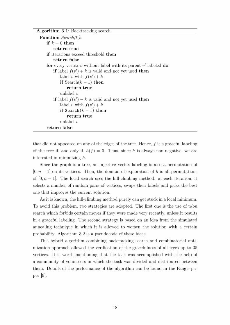
Algorithm 3.1: Backtracking searchFunction Search(k):
if k = 0 thenreturn true
if iterations exceed threshold thenreturn false
for every vertex v without label with its parent v′ labeled doif label f(v′) + k is valid and not yet used then
label v with f(v′) + kif Search(k − 1) then
return trueunlabel v
if label f(v′)− k is valid and not yet used thenlabel v with f(v′) + kif Search(k − 1) then
return trueunlabel v
return false
that did not appeared on any of the edges of the tree. Hence, f is a graceful labelingof the tree if, and only if, h(f) = 0. Thus, since h is always non-negative, we areinterested in minimizing h.
Since the graph is a tree, an injective vertex labeling is also a permutation of[0, n − 1] on its vertices. Then, the domain of exploration of h is all permutationsof [0, n − 1]. The local search uses the hill-climbing method: at each iteration, itselects a number of random pairs of vertices, swaps their labels and picks the bestone that improves the current solution.
As it is known, the hill-climbing method purely can get stuck in a local minimum.To avoid this problem, two strategies are adopted. The first one is the use of tabusearch which forbids certain moves if they were made very recently, unless it resultsin a graceful labeling. The second strategy is based on an idea from the simulatedannealing technique in which it is allowed to worsen the solution with a certainprobability. Algorithm 3.2 is a pseudocode of these ideas.
This hybrid algorithm combining backtracking search and combinatorial opti-mization approach allowed the verification of the gracefulness of all trees up to 35vertices. It is worth mentioning that the task was accomplished with the help ofa community of volunteers in which the task was divided and distributed betweenthem. Details of the performance of the algorithm can be found in the Fang’s pa-per [9].
18

Algorithm 3.2: Local search using metaheuristicslet f be the vertex labeling corresponding to the identity permutationv ← h(f)while v 6= 0 do
randomly choose 2n pairs of verticesforeach pair of vertices (x, y) chosen do
swap the values of f(x) and f(y)evaluate h for the modified labelingswap back f(x) with f(y)
choose the pair (x, y) that minimizes hlet f ′ be the labeling obtained by swapping f(x) with f(y)v′ ← h(f ′)if f(x), f(y) was not swapped in the last bn/3c iterations then
if v > v′ thenswap f(x) with f(y), and update v
elsewith probability p, swap f(x) with f(y), and update v
else if v′ = 0 thenswap f(x) with f(y), and update v
return f
3.3 Relaxed versions
Relaxed versions of graceful labeling have been studied for as long as gracefullabeling itself. Rosa himself introduced together with graceful labeling some variantsof it, both stronger and weaker versions of graceful labeling.
Usually, one only consider relaxed versions when the graph is not graceful. How-ever, here we consider a couple of relaxed versions of graceful labeling for trees, and,with the purpose of getting closer to the Graceful Tree Conjecture, the goal has beenin trying to improve bounds for these labelings.
Probably, the following relaxed graceful labelings are the most intuitive ones.
1. Edge-relaxed : fγ can be non-injective.
2. Vertex-relaxed : f can be non-injective (fγ must still be injective).
3. Range-relaxed : f : V (G)→ [0, k] for some k ≥ m.
Bounds have been established for all these three versions. Rosa and Širáň [22]showed that every tree has a edge-relaxed graceful labeling with at least 5m/7
different edge labels. Van Bussel [25] showed two results, one concerning vertex-relaxed graceful labeling of trees and the other concerning the range-relaxed gracefullabeling of trees, which we present next.
19

Theorem 3.6. Every tree T has a range-relaxed graceful labeling with vertex labelsin the range [0, 2m− diam(T )].
Proof. Let T = (V,E) be a tree and v0 ∈ V , and consider the tree T rooted atv0. Also consider that the longest path from v0 is at the leftmost in a planarrepresentation of T . Let the length of this path be `, the vertices of the path bev0, v1, . . . , v`, and hi be the number of vertices at level i. The following constructionprovides a vertex labeling for T in the range [0, 2m− `].
1. Label v0 temporarily with α and v1 with α+1. After labeling all vertices, weshift all labels by a constant so that the smallest value is 0.
2. For i > 1, label vi as follows:
f(vi) =
f(vi−2)− hi−2 − hi−1 + 1 = α−∑i−1
j=0 hj +i2
if i is even
f(vi−2) + hi−2 + hi−1 − 1 = α +∑i−1
j=0 hj −i−12
if i is odd
3. At each level i, consider the order in which the vertices are represented in theplace. Label the k-th vertex ui,k at level i, k ∈ [0, hi − 1], as follows:
f(ui,k) =
f(vi)− k if i is even
f(vi) + k if i is odd
Figure 3.3: Labeling of Theorem 3.6 at level i even.
It is clear that all vertex labels are distinct: as we go from top to bottom, leftto right, on even levels they are decreasing, and on odd levels they are increasing.Moreover, all edge labels are distinct. Indeed, the edge labels are increasing as wego from top to bottom, left to right.
20

Consider two edges uiui+1 and wiwi+1 where ui and wi are at the same level i.If i is even, then f(ui) > f(wi) and f(ui+1) < f(wi+1). Then,
fγ(uiui+1) = f(ui+1)− f(ui) < f(wi+1)− f(wi) = fγ(wiwi+1)
Analogously, the same holds if i is odd.Now, let ui and ui+1 be the rightmost vertices at levels i and i+ 1, respectively,
and consider the edge uiui+1, which is not necessarily an edge of the tree. By whatwe just showed, it has the largest edge label from level i to i + 1. So, it suffices toshow that fγ(uiui+1) < fγ(vi+1vi+2), since vi+1vi+2 has the smallest edge label fromlevel i+ 1 to i+ 2. Assuming i even, we have
fγ(uiui+1) = f(ui+1)− f(ui)
= f(vi+1) + hi+1 − 1− (f(vi)− hi + 1)
< f(vi+1)− (f(vi)− hi − hi+1 + 1)
= fγ(vi+1vi+2)
Again, the same holds if i is odd by an analogous proof.Finally, we check that the labels are inside the range. Let fmax and fmin be the
maximum and the minimum vertex labels, respectively. If ` is even, then the largestvertex label is at level `− 1 and the smallest one is at level `.
fmax = f(v`−1) + h`−1 − 1
= α +`−2∑j=0
hj −`− 2
2+ h`−1 − 1
= α +m+ 1− h` −`
2
fmin = f(v`)− h` + 1
= α−`−1∑j=0
hj +`
2− h` + 1
= α−m+`
2
fmax − fmin = α +m+ 1− h` −`
2−(α−m+
`
2
)= 2m− l − h` + 1
≤ 2m− l
Thus, if we choose our root as one of the end vertices of a longest path in thetree, we obtain a range-relaxed graceful labeling in the range [0, 2m−diam(T )].
21

Theorem 3.7. Every tree T has a vertex-relaxed graceful labeling with more than n2
distinct vertex labels.
Instead of proving Theorem 3.7 directly, Van Bussel proved a stronger result.Before that, we must define the following labeling. We say a vertex labeling f islocally bipartite if there is a bipartition of V (G) = A ∪B such that
1. ∀u ∈ A ∀v ∈ N(u) : f(u) < f(v)
2. ∀v ∈ B ∀u ∈ N(v) : f(u) < f(v)
Note that if a graph G admits such labeling, then G must be bipartite.
Theorem 3.8. Let T = (V,E) be a tree with a bipartition of V = A ∪ B, and letv ∈ A be an arbitrary vertex. Then, there exists a vertex-relaxed graceful labeling fof T satisfying the following properties:
1. f is locally bipartite;
2. f(v) = 0;
3. f(x) 6= f(y) for all x, y ∈ B.
Proof. We prove by induction on n. For n = 1 and n = 2, it is clear that suchlabeling exists. Suppose n > 2, and let v be an arbitrary vertex of T . We divide intwo cases.
Case 1. Assume d(v) ≥ 2. Since v has at least two adjacent vertices, we cansplit v into two vertices v1 and v2 and obtain two trees T1 and T2 strictly smallerthan T such that T is the union of T1 and T2 by identifying v1 with v2. By induction
Figure 3.4: Splitting the tree at the vertex v.
hypothesis, T1 has a bipartition V (T1) = A1 ∪B1 with v1 ∈ A1 and a vertex-relaxedgraceful labeling f1 satisfying those properties with respect to v1. Similarly, we haveA2, B2, and f2 for T2. Thus, if m1 = |E(T1)|, the labeling f of T defined by
f(u) =
f1(u) if u ∈ V (T1)
f2(u) if u ∈ A2
f2(u) +m1 if u ∈ B2
22

is the required labeling.
1. f(v) = f(v1) = f(v2) = 0
2. Since we are adding a constant to all vertex labels in B2, f2 remains locallybipartite. Hence, f is also locally bipartite.
3. The edge labels in T1 remains the same in T and those in T2 are shifted by m1,generating edge labels {m1 + 1, . . . ,m1 +m2}. Hence, f is a vertex-relaxedgraceful labeling of T .
4. All vertex labels in B1 and B2 are distinct. Thus,
min{f2(B2)}+m1 ≥ m1 + 1 > m1 = max{f1(B1)}
and we have that all vertex labels in B1 ∪B2 are distinct.
Case 2. Assume d(v) = 1. Let w be the adjacent vertex of v. Since n ≥ 3, wehave d(w) ≥ 2. Let r1, r2, . . . , rk, where k = d(w)− 1, be the vertices adjacent to wexcept for v. Let the trees of T − w rooted at ri be Ti with mi edges, bipartition(Ai, Bi), and ri ∈ Ai.
Since Ti is smaller than T by at least 2 vertices, by induction hypothesis, Ti hasa vertex-relaxed graceful labeling fi satisfying those properties with respect to ri.The labeling f of T defined below is as required.
f(v) = 0
f(w) = m
f(u) =
fi(u) + i if u ∈ Aifi(u) +
∑i−1j=1mj + i if u ∈ Bi
For the verification, let us denote Mi =∑i−1
j=1mj.
1. For each tree Ti, f adds the constant i to all vertices and also adds Mi to thevertices in Bi, which means that f is locally bipartite in Ti. And, since w getsthe largest vertex label possible, we have that f is locally bipartite in T .
2. For each tree Ti, f shifts all edge labels by Mi. Together with edges incidentwith w, which has labels {m,m− 1, . . . ,m− k}, we have that each edge labelin [1,m] appears in some edge. Hence, f is a vertex-relaxed graceful labeling.
3. It is clear that in each Bi, all vertices have different labels. And, sincemax{f(Bi)} =Mi+mi+ i < Mi+1+ i+1 = min{f(Bi)}, we have that all la-bels in
⋃ki=1Bi are distinct, and the maximum of these labels isMk+mk+k =
m− 1. Hence, all the vertex labels in B = {w} ∪⋃ki=1Bi are distinct.
23

Therefore, every tree T admits a vertex-relaxed graceful labeling satisfying thoseproperties. If we take A as the smallest set of the bipartition of T , we have |B| ≥ n
2.
And, since the vertex label 0 can not appear in B, we have at least n2+ 1 distinct
vertex labels, as required in Theorem 3.7.
Although it is clear that every graph admits an edge-relaxed and a range-relaxedgraceful labelings, not all graphs have a vertex-relaxed graceful labeling [25]. Fur-thermore, it is still unknown a connected non-graceful graph that has a vertex-relaxed graceful labeling.
24

Chapter 4
Generalized Cone Graphs
In Chapter 2, we presented the gracefulness of some graph classes and how toconstruct bigger graceful graphs from smaller ones. In this chapter, we generalizethe wheel graphs, also known as cone graphs, and study its gracefulness. This graphclass was first studied by Bhat-Nayak and Selvam [6] in 2003 and not much progresshas been made since then.
A generalized cone graph is the join of a cycle graph Cp and an independent setIq, where p ≥ 3 and q ≥ 0. For instance, for q = 0 and q = 1, we simply have thecycle graphs and the wheel graphs, respectively.
Throughout this chapter, we denote the vertices of the generalized cone graphs asV (Cp + Iq) = {u0, u1, . . . , up−1, v0, v1, . . . , vq−1} where uk ∈ V (Cp), ukuk+1 ∈ E(Cp)for 0 ≤ k < p and up = u0, and vk ∈ V (Iq). Also, from now on, we simply callgeneralized cone graphs as cone graphs.
The first result we show is concerning the non-graceful cone graphs. As we said inChapter 2, the only useful theoretical tool for proving the non-existence of gracefullabeling for a given graph is the parity condition, which only applies to Euleriangraphs. Thus, applying the parity condition to Eulerian cone graphs, the followingholds.
Proposition 4.1. The cone graph Cp + Iq is not graceful for p ≡ 2 (mod 4) andq ≡ 0 (mod 2).
Proof. For p ≡ 2 (mod 4) and q ≡ 0 (mod 2), the cone Cp + Iq is Eulerian sincethe degree of every vertex is even (cf. [7]), and it has m = p(q + 1) edges. Writingp = 4s + 2 and q = 2t, we have m = (4s + 2)(2t + 1) ≡ 2 (mod 4). Hence, by theparity condition, Cp + Iq is not graceful.
25

4.1 Graceful cones
For q = 0 and q = 1, we have the cycle graphs and the wheel graphs, respec-tively, and their gracefulness is already characterized in Chapter 2. For q = 2, wehave the double cones, and it is still an open problem to characterize them. ByProposition 4.1, the double cone Cp + I2 is not graceful for p ≡ 2 (mod 4), and sofar they are the only non-graceful double cones [6, 11, 19].
012
1
26
9
1
2
3 4
56
7
89
10
1112
Figure 4.1: Graceful labeling of C4 + I2.
For the general case, Bhat-Nayak and Selvam [6] proved the following theorem.
Proposition 4.2. The cone graph Cp + Iq is graceful for p ≡ 0, 3 (mod 12) andq ≥ 1.
For the proof of Proposition 4.2, Bhat-Nayak and Selvam introduced a new graphlabeling and showed a more general result similar to Theorem 2.7.
A vertex labeling f of a graph G with n vertices is said to be a special labelingif it satisfies the following conditions:
1. For every i ∈ [1, n], there exists a vertex ui ∈ V (G) such that f(ui) is either2i− 1 or 2i.
2. Im(fγ) = [1, 2n] \ Im(f).
3. If f(x) and fγ(xy) are odd, then f(x) < f(y).
Note that conditions 1 and 2 imply that the number of vertices must be the sameas the number of edges, i.e., n = m.
Theorem 4.3. If a graph G has a special labeling, then the graph G+ Iq is gracefulfor all q ≥ 1.
Proof. Let G be a graph on p vertices and f be a special labeling of G. Define thevertex labeling g for G + Iq as follows, where V (G) = {u1, . . . , up} and V (Iq) =
{v1, . . . , vq}:
26

g(vj) = j − 1
g(ui) =
i(q + 1) if f(ui) = 2i
i(q + 1)− 1 if f(ui) = 2i− 1
We claim g is a graceful labeling of G+Iq. As noted before, since G has a speciallabeling, G has p edges. Thus, the number of edges of G + Iq is p + pq. Clearly,g : V (G+ Iq)→ [0, p(q + 1)] and it is injective. So, we have to prove that gγ is onto[1, p(q + 1)]. For that, we show that for each i ∈ [1, p] and j ∈ [1, q + 1], there is anedge e with gγ(e) = (i− 1)(q + 1) + j.
Consider a pair (i, j). Since f is a special labeling of G, by condition 1, there isa vertex ui ∈ V (G) with f(ui) = 2i− 1 or f(ui) = 2i.
Case 1. f(ui) = 2i− 1 and 1 ≤ j ≤ q.We have g(ui) = i(q+1)−1 and g(vq−j+1) = q− j. Since q− j < i(q+1)−1,the edge label on uivq−j+1 is i(q + 1)− 1− (q − j) = (i− 1)(q + 1) + j.
Case 2. f(ui) = 2i− 1 and j = q + 1.By condition 2, there is an edge e = xy ∈ E(G) with fγ(xy) = 2i. Hence, f(x)and f(y) have the same parity. Suppose f(x) = 2a+r and f(y) = 2b+r, wherer ∈ {0, 1} is the parity. Then, fγ(xy) = 2i = |(2a+ r)− (2b+ r)| = 2|a− b|,and i = |a − b|. Therefore, gγ(xy) = |(a(q + 1) − r) − (b(q + 1) − r)| =(q + 1)|a− b| = i(q + 1) = (i− 1)(q + 1) + (q + 1)
Case 3. f(ui) = 2i and 2 ≤ j ≤ q + 1.We have g(ui) = i(q+1) and g(vq−j+2) = q− j+1. Since q− j+1 < i(q+1),the edge label on uivq−j+2 is i(q + 1)− (q − j + 1) = (i− 1)(q + 1) + j.
Case 4. f(ui) = 2i and j = 1.By condition 2, there is an edge e = xy ∈ E(G) with fγ(xy) = 2i− 1. Now,f(x) and f(y) have different parities. Without loss of generality, suppose f(x)odd and let f(x) = 2a−1 and f(y) = 2b. By condition 3, we have f(x) < f(y)
which implies g(x) < g(y). Thus, fγ(xy) = 2i − 1 = 2b − (2a − 1) impliesi−1 = b−a. Finally, gγ(xy) = b(q+1)− (a(q+1)−1) = (b−a)(q+1)−1 =
(i− 1)(q + 1)− 1.
Thus, we have proved that Im(gγ) = [1, p(q + 1)] and therefore g is a gracefullabeling of G+ Iq.
We do not present here the complete proof of Proposition 4.2. Here, we onlyshow a partial result which says that C24k + Iq is graceful. For that, Bhat-Nayakand Selvam proved the following lemmas.
27

Lemma 4.4. For k ≥ 2, P4k−3 has a vertex labeling f such that Im(f) = [k+2, 2k]∪[2k + 3, 3k + 1] ∪ [5k + 1, 7k − 1], Im(fγ) = [2k + 1, 6k − 4], and the end verticesreceive the labels 5k + 1 and 7k − 1.
Proof. Let P4k−3 = u1u2 · · ·u4k−3 and define the vertex labeling f as follows:
f(u2i−1) = 5k + i for 1 ≤ i ≤ 2k − 1
f(u2i) = k + 2 for i = 1
= 3k + 3− i for 2 ≤ i ≤ k
= 3k + 1− i for k + 1 ≤ i ≤ 2k − 2
Now, it is easy to verify directly that Im(fγ) = [2k + 1, 6k − 4].
Remark 4.1. For k = 1, consider the single vertex of P1 labeled with 6.
Lemma 4.5. For k ≥ 1, P8k−1 has a vertex labeling f such that Im(f) = [1, k] ∪[k + 2, 8k], Im(fγ) = [1, 8k − 2], and the end vertices receive the labels 2k + 1 and8k.
Proof. Let P8k−1 = u1u2 · · ·u8k−1 and define the vertex labeling f as follows:
f(u1) = 2k + 1
f(u2i+1) = 4k + 1 + i for 1 ≤ i ≤ k
f(u2i) = 4k + 2− i for 1 ≤ i ≤ k
f(u8k+1−2i) = 8k + 1− i for 1 ≤ i ≤ k + 2
f(u8k−2) = 2k + 2
f(u8k−2−2i) = i for 1 ≤ i ≤ k
Thus, we labeled the vertices u1, . . . , u2k+1, u6k−3, . . . , u8k−1 with labels in [1, k]∪[2k + 1, 2k + 2] ∪ [3k + 2, 5k + 1] ∪ [7k − 1, 8k], and obtained edge labels in [1, 2k] ∪[6k− 3, 8k− 2]. For the remaining subpath u2k+1u2k+2 · · ·u6k−3, label it as given byLemma 4.4 to obtain the desired labeling.
Lemma 4.6. For k ≥ 1, P8k−1 has a vertex labeling g such that Im(g) = {16k +
2, 16k+ 4, . . . , 18k} ∪ {18k+ 4, 18k+ 6, . . . , 32k}, Im(fγ) = {2, 4, . . . , 16k− 4}, andthe end vertices receive the labels 20k + 2 and 32k.
Proof. Let f be the vertex labeling obtained from Lemma 4.5. Then, defining g asg(u) = 2f(u) + 16k gives the required labeling.
Lemma 4.7. For k ≥ 1, P16k+3 has a vertex labeling f such that Im(f) = {1, 3, . . . ,16k − 1, 18m + 2, 20k + 2, 32k, 32k + 2, . . . , 48k}, Im(fγ) = {16k − 2, 16k, 16k + 1,
16k + 3, . . . , 48k − 1}, and the end vertices receive the labels 20k + 2 and 32k.
28

Proof. Let P16k+3 = u1u2 · · ·u16k+3 and define the vertex labeling f as follows:
f(u2i−1) = 20k + 2 for i = 1
= 48k + 4− 2i for 2 ≤ i ≤ 8k + 2
f(u2i) = 2i− 1 for 1 ≤ i ≤ 7k
= 18k + 2 for i = 7k + 1
= 2i− 3 for 7k + 2 ≤ i ≤ 8k + 1
Now, it is easy to verify that Im(fγ) is as required.
Proposition 4.8. The cone graph C24k + Iq is graceful for all k ≥ 1.
Proof. Consider P8k−1 and P16k+3 labeled as given by Lemmas 4.6 and 4.7 respec-tively. By joining the paths by identifying the end vertices with the same label,we get a C24k with a vertex labeling f such that Im(f) = {1, 3, . . . , 16k − 1, 16k +
2, 16k+4, . . . , 48k} and Im(fγ) = {2, 4, . . . , 16k, 16k+1, 16k+3, . . . , 48k− 1}. Fur-thermore, the largest odd vertex label is less than the smallest even vertex label.Therefore, f satisfies all three conditions of being a special labeling for C24k.
Therefore, by Theorem 4.3, C24k + Iq is graceful.
For the proof of Proposition 4.2, Bhat-Nayak and Selvam proved not only Propo-sition 4.8, but also that Cp + Iq is graceful for p ≡ 3, 12, 15 (mod 12), each of themfollowing the same strategy as shown before: prove the existence of a specific vertexlabeling of some specific paths and then join their end vertices to form a cycle graph.
Besides Proposition 4.2, Bhat-Nayak and Selvam also proved the following propo-sition.
Proposition 4.9. The cone graph Cp + Iq is graceful for p = 7, 11, 19 and q ≥ 1.
Proof. The following vertex labelings are special labelings for their respective cycle.C7: 1, 14, 5, 7, 10, 4, 12.C11: 1, 22, 5, 18, 7, 15, 9, 12, 14, 4, 20.C19: 1, 36, 3, 34, 5, 32, 7, 30, 12, 26, 16, 22, 20, 24, 13, 28, 9, 17, 38.
Brundage [8] also worked on this problem and showed the following result.
Proposition 4.10. The cone graphs C5 + Iq and C8 + Iq are graceful for all q ≥ 1.
Proof. Brundage gives a graceful labeling f : V → [0,m] for each case.For C5+Iq, label the vertices of C5 with 0,m,m−3, 3,m−1 consecutively along
the cycle, where m = 5(q + 1) is the total number of edges. Now, label the verticesof Iq as follows:
f(vk) =
2 if k = 0
5k + 3 if k = 1, 2, . . . , q − 1
29

Thus, for 0 < k < q, as 3 < 5k + 3 < m− 3, the incident edges of vk have labels5k+3,m− (5k+3), (m− 3)− (5k+3), 5k, (m− 1)− (5k+3), which are all distinctsince they have different residues modulo 5:
5k + 3 ≡ 3 (mod 5)
m− (5k + 3) ≡ 2 (mod 5)
(m− 3)− (5k + 3) ≡ 4 (mod 5)
5k ≡ 0 (mod 5)
(m− 1)− (5k + 3) ≡ 1 (mod 5)
It is now easy to see that the labels in the edges incident with vk, 0 < k < q, coverthe whole interval [4,m − 7]. Along with the labels of the edges in C5 (m, 3,m −6,m− 4,m− 1) and those incident with v0 (2,m− 2,m− 5, 1,m− 3), all the labelsin [1,m] appear exactly once. Thus, f is a graceful labeling of C5 + Iq.
For C8 + Iq, label the vertices of C8 with 0,m, 2, 3,m− 2, 1,m− 3,m− 1 alongthe cycle, where m = 8(q + 1), and label each vk in Iq with 4k + 6. The proof thatthis is indeed a graceful labeling is analogous to the previous case.
Remark 4.2. Note that the graceful labeling for some families of cone graphs is oftennot unique. For instance, a graceful labeling for C8 + Iq distinct from the one givenby Brundage goes as follows. Label C8 with 0,m, m
2, 3m
4+1, m
2+1, 3m
4, m
4− 1,m− 1,
and label Iq with 2k + 2 for 0 ≤ k < q, where m = 8(q + 1).
Brundage [8] organized the gracefulness of cone graphs in a table (see Table 4.1)and made a conjecture characterizing this class.
Conjecture 4.1 (Brundage, 1994). The generalized cone graph Cp + Iq is gracefulif, and only if, the parity condition holds.
q
p3, 4 5 6 7, 8 9 10 11, 12 13 14 comments
0 Y N N Y N N Y N N Y iff p ≡ 0, 3 (mod 4)
1 Y Y Y Y Y Y Y Y Y Y ∀p2 Y Y N Y Y N Y ? N ?, N ∀p = 6 + 4k
3 Y Y Y Y Y ? Y ? ? ?4 Y Y N Y Y N Y ? N ?, N ∀p = 6 + 4k
5 Y Y ? Y ? ? Y ? ? ?6 Y Y N Y ? N Y ? N ?, N ∀p = 6 + 4k
7 Y Y ? Y ? ? Y ? ? ?8 Y Y N Y ? N Y ? N ?, N ∀p = 6 + 4k
9 Y Y ? Y ? ? Y ? ? ?
comments Y Y∀q ≥ 1
?,N ∀qeven
Y ??,
N ∀qeven
Y ??,
N ∀qeven
?,N ∀p = 6 + 4k, q evenY ∀p ≡ 0, 3 (mod 12)
Table 4.1: Gracefulness of Cp + Iq (updated as of 2014).
30

4.2 Computational results
Questioning the validity of Conjecture 4.1, we started looking for counterexam-ples, i.e., find a cone graph for which the parity condition does not hold and it isnot graceful. For this task, a backtracking search algorithm similar to the Fang’salgorithm presented in Chapter 3 was implemented.
The strategy is the same as in Fang’s algorithm: it tries to create a new edgelabel at each iteration by labeling a not yet labeled vertex. For reducing the searchtree, some optimizations were made due to the inherent symmetries of cone graphs.The following observations eliminate most of search through equivalent labelingsgiven by the symmetries of the graph.
Force f(u0) = 0 without loss of generality. Since the edge labeling function fγis a bijection, i.e., in a graceful labeling, every possible edge label from 1 to m mustappear as a label of some edge, and an edge label is obtained as the absolute value ofthe difference of the labels of its incident vertices, it follows that the vertices labeled0 and m must be adjacent in the graph. Otherwise, no edge would be assigned labelm. Furthermore, since all edges are incident with at least one vertex of the cycle,one of the vertices of the cycle must be labeled 0 or m. By symmetry, let u0 bethat vertex. Now, the complementarity property allows us to assume without lossof generality that f(u0) = 0.
Just two candidate recipients for vertex label m. Assuming f(u0) = 0, thevertex label m must be assigned to a vertex that is adjacent to u0, i.e., to eitheru1, up−1 or vk for some k ∈ [0, q − 1]. Again owing to the symmetries in both thecycle and the independent set, we can narrow down our options, without loss ofgenerality, to only two among those vertices, say u1 and v0.
Constrained recipients for edge label m−1. If, in the previous step, we chosevertex u1 to receive label m, then, because we had already assigned label 0 to vertexu0, the edge label m − 1 can only appear on an edge that is incident with eitheru1 (a neighbor of u1 would receive label 1) or u0 (a neighbor of u0 would receivelabel m − 1). Owing to the symmetries (rotation, reflection) of the cycle and thecomplementarity property, these two cases are actually equivalent. We can thereforeconsider, without loss of generality, that the edge labeled m−1 will be incident withu1. We must now pick a neighbor of vertex u1 to assign label 1. Since vertex u0is already labeled with 0, the possible neighbors are u2 or vk. However, by thesymmetry of the independent set, we can consider v0 as the sole candidate to receivelabel 1, and our search is limited to just two cases. If, on the other hand, we chosevertex v0 to receive label m, then we must either assign label m − 1 to a neighbor
31

of u0 (namely u1 or v1 without loss of generality), or assign label 1 to a neighbor ofv0 (namely uk, where we can impose 1 ≤ k ≤ bp
2c owing to the reflection symmetry
of the cycle).
Establish an order of labeling in Iq. Since all vertices in the independent setare indistinguishable between themselves (both from the standpoint of some vertexin the independent set, since there are no edges between any of them, and from thestandpoint of some vertex in the cycle, since each vertex in the cycle is adjacent toall vertices in the independent set), we may assume an order in which the verticesof Iq are labeled. This prevents looking for labelings that are identical up to apermutation of the vertices in Iq.
Putting together these ideas, Algorithm 4.1 shows a pseudocode for the back-tracking search algorithm to find a graceful labeling for a cone graph.
Algorithm 4.1: Backtracking search for generalized cone graphsFunction Search(upper):
if upper = 0 thenreturn true
lbl← largest edge label ≤ upper not present yetforeach pair (k, kc) with |k − kc| = lbl do
if both k and kc are not vertex labels yet thenforeach edge uv with both ends unlabeled do
label u with k and v with kcif Check() and Search(lbl − 1) then return truelabel u with kc and v with kif Check() and Search(lbl − 1) then return trueunlabel u and v
elselet k be the unused vertex label and u be the vertex with label kcif u ∈ V (Cp) then
foreach v ∈ N(u) ∩ V (Cp), v unlabeled dolabel v with kif Check() and Search(lbl − 1) then return trueunlabel v
if there are unlabeled vertex in Iq thenv ← next unlabeled vertex from Iqlabel v with kif Check() and Search(lbl − 1) then return trueunlabel v
elseforeach v ∈ V (Cp), v unlabeled do
label v with kif Check() and Search(lbl − 1) then return trueunlabel v
32

The function Check in the pseudocode checks if the current labeling is valid, i.e.,it checks if there are no repeated edge or vertex labels. Unlike Fang’s backtrackingsearch algorithm, this check is necessary here because labeling a vertex can createmore than just one edge label. So, a verification is necessary every time we label anew vertex before continuing the search.
Running the search for a graceful labeling for C6 + I5, the smallest cone graphwhich was still unknown to be graceful or not, the algorithm returned no possiblegraceful labeling, refuting, therefore, Brundage’s conjecture. Moreover, the algo-rithm did not find a graceful labeling for C6 + Iq with 5 ≤ q ≤ 35. Notice that weare only interested in odd values of q since, for even values, the parity conditionalready settles that C6 + Iq is not graceful.
Searching for more non-graceful cone graphs, it makes sense to look for conegraphs Cp+ Iq with p ≡ 2 (mod 4) as they are the only ones that, together with aneven q, are not graceful by the parity condition. Then, the next subclass to searchfor non-graceful cones is C10 + Iq. We found that C10 + I3 and C10 + I5 are graceful.However, the algorithm returned no graceful labeling for C10 + Iq with 7 ≤ q ≤ 25.A similar result was gotten with p = 14: the cones C14+I3 and C14+I5 are graceful,but the cones C14 + I7 and C14 + I9 are not. The following propositions summarizethese results.
Proposition 4.11. The cone graphs C10 + Iq and C14 + Iq are graceful for q = 3, 5.
Proof. We have the following labelings where the first p labels are from the cycleand the last q are from the independent set.
C10 + I3: 0, 40, 25, 3, 33, 13, 6, 29, 10, 21; 37, 38, 39.C10 + I5: 0, 27, 1, 57, 14, 13, 2, 16, 3, 15; 23, 32, 51, 55, 60.C14 + I3: 0, 56, 6, 1, 28, 5, 2, 30, 34, 3, 33, 11, 22, 55; 40, 47, 54.C14 + I5: 0, 84, 33, 17, 82, 34, 47, 54, 64, 68, 69, 32, 49, 83; 2, 5, 8, 11, 14.
Proposition 4.12. The cone graphs C6 + Iq, 5 ≤ q ≤ 35, C10 + Iq, 7 ≤ q ≤ 25,C14 + I7, and C14 + I9 are not graceful.
Proof. Proven computationally.
Proposition 4.12 not only disproves Conjecture 4.1, but also gives a strongerfeeling about how the non-gracefulness of generalized cone graphs behaves, fromwhich we conjecture the following.
Conjecture 4.2. For every p ≡ 2 (mod 4), there exists a qp > 1 such that the conegraph Cp + Iq is not graceful for all q ≥ qp.
One might think of trying to prove it computationally, implementing an algo-rithm to do something similar to the proof of Proposition 2.2, exhausting all pos-sibilities for all values of q greater than a threshold. However, as it was noted,
33

the running times of the algorithm to establish the non-gracefulness were growingexponentially, which indicates that it is not possible to prove it in this way.
Besides the non-graceful cone graphs, we also searched for new families of coneswhich are graceful. We have seen two approaches to tackle this class: fixing the sizeof the independent size or fixing the size of the cycle. By taking the last one, westarted to find graceful labelings for C9 + Iq, the smallest family of this kind whichwas still open, and tried to find a pattern in the labelings while increasing the sizeof the independent size. As seen in Proposition 4.10, a simple rule could be possible,and indeed we found a scheme of labeling, not only for C9+ Iq, but also for C13+ Iq.
Proposition 4.13. The cone graphs C9+ Iq and C13+ Iq are graceful for all q ≥ 1.
Proof. For C9+Iq, label the vertices of C9 with 0,m, 5,m−7, 3,m−8,m−3, 4,m−2along the cycle, where m = 9(q + 1) is the number of edges, and label Iq as follows:
f(vk) =
1 if k = 0
9k + 4 if k = 1, 2, . . . , q − 1
For C13 + Iq, label the vertices of C13 as 0,m,m− 8, 6,m− 9, 10,m− 6, 7,m−4,m−7, 5,m−1,m−3 along the cycle, where m = 13(q+1) is the number of edges,and label Iq as follows:
f(vk) =
1 if k = 0
13k + 4 if k = 1, 2, . . . , q − 1
As for the verification, since it is analogous to the proof of Proposition 4.10, itis omitted.
On the other hand, finding a pattern after having fixed the size of the independentset (and allowing the size of the cycle to grow freely) seems to be much harder. Forinstance, it seems that, for p > 5 and p ≡ 1 (mod 4), the cone graph Cp + Iq has agraceful labeling f such that f(v0) = 1 and f(vk) = pk + 4 for 1 ≤ k < q, as it canbe seen in Proposition 4.13; we have also verified it for several cones with p = 17
and p = 21. However, no pattern has been found for the cycles. Another example isthe family of cone graphs Cp + Iq with p ≡ 0 (mod 4): each of them seems to havea graceful labeling with f(vk) = p
4(k + 1) for 0 ≤ k < q. That is known to be true
for p = 4 [6], and now p = 8 (see Remark 4.2); we have also verified that severalcones with p = 12, 16, 20 admit such labeling.
Table 4.2 summarizes the current state of the gracefulness of generalized conegraphs for small values and gives a comment for the state of each row and column.
34

q
p3, 4 5 6 7, 8 9 10 11, 12 13 14 comments
0 Y N N Y N N Y N N Y iff p ≡ 0, 3 (mod 4)
1 Y Y Y Y Y Y Y Y Y Y ∀p2 Y Y N Y Y N Y Y N ?, N ∀p = 6 + 4k
3 Y Y Y Y Y Y Y Y Y ?4 Y Y N Y Y N Y Y N ?, N ∀p = 6 + 4k
5 Y Y N Y Y Y Y Y Y ?6 Y Y N Y Y N Y Y N ?, N ∀p = 6 + 4k
7 Y Y N Y Y N Y Y N ?8 Y Y N Y Y N Y Y N ?, N ∀p = 6 + 4k
9 Y Y N Y Y N Y Y N ?10 Y Y N Y Y N Y Y N ?, N ∀p = 6 + 4k
11 Y Y N Y Y N Y Y ? ?
comments Y Y∀q ≥ 1
?,N ∀qeven
Y Y∀q ≥ 1
?,N ∀qeven
Y Y∀q ≥ 1
?,N ∀qeven
?,N ∀p = 6 + 4k, q evenY ∀p ≡ 0, 3 (mod 12)
Table 4.2: Gracefulness of Cp + Iq (shaded entries are new results).
35

Chapter 5
Conclusion
The graceful labeling of graphs has been a topic of research for 50 years andit still has many properties to be found. Although its primary interest was thegraceful labeling of trees in order to solve Ringel’s conjecture, graceful labeling ofgraphs gained over the years its own beauty and interest.
This work gives a brief overview of the subject, presenting not only theoreticalresults from the literature, but also some computational results. Furthermore, wegive some contributions to this problem.
In Chapter 2, the problem is presented, as well as the gracefulness of some rathersimple graph classes like cycles and wheels. We also show necessary conditions tothe existence of a graceful labeling for a graph, and two methods of constructinggraceful graphs. In particular, one of them shows that any graph is an inducedsubgraph of some graceful graph.
In Chapter 3, we focus on graceful labeling of trees, more specifically, on differentways to approach the Graceful Tree Conjecture. The first one tackle the trees bylimiting the diameter by introducing the transfer operation to modify a tree keepingit graceful. The second one reinforces the conjecture by showing computationallythat all trees up to 35 vertices are graceful. Finally, we present some relaxed versionof graceful labeling in which the better the bound, the closer to the conjecture weare.
In Chapter 4, we move our focus to generalized cone graphs. Their graceful-ness was first tackled by Bhat-Nayak and Selvam, although some particular caseswere already known. Later, Brundage also worked on this graph class and made aconjecture characterizing the gracefulness of cone graphs.
We tackled the gracefulness of cone graphs computationally and were able todisprove Brundage’s conjecture. We also establish the gracefulness of new familiesof cone graphs and make a new conjecture regarding the non-graceful cone graphs.
For future work on the subject, we could consider looking for a way to proveConjecture 4.2, or even characterize the gracefulness of generalized cone graphs. As
36

we showed in Chapter 4, it seems that Cp+ Iq is graceful for p ≡ 0, 1, 3 (mod 4) andq ≥ 1. For p ≡ 2 (mod 4), our conjecture says there is a qp > 1 such that the conegraph is not graceful for all q ≥ qp. If, moreover, we could find out the parameterqp for each p ≡ 2 (mod 4), we would have a characterization of the gracefulness ofgeneralized cone graphs.
Another class of interest is the class of trees, being the main open class on thistopic. It is already settled that many classes of trees are graceful, but also thereare many classes, even simple ones like lobsters, that are still open. Finally, anotherapproach to the problem is to relax the conditions of graceful labelings and findnearly graceful labelings. This approach by approximating the labeling is also atopic of research for both trees and graphs in general.
37

Bibliography
[1] Acharya, B. D. Construction of certain infinite families of graceful graphs froma given graceful graph. Defence Science Journal 32, 3 (1982), 231–236.
[2] Aldred, R. E. L., and McKay, B. D. Graceful and harmonious labellings oftrees. Bulletin of the Institute of Combinatorics and its Applications 23(1998), 69–72.
[3] Arumugam, S., and Bagga, J. Graceful labeling algorithms and complexity- a survey. Journal of the Indonesian Mathematical Society (2011), 1–9.
[4] Bermond, J.-C. Graceful graphs, radio antennae and French windmills. InGraph Theory and Combinatorics (1979), vol. 34 of Research Notes inMathematics, pp. 18–37.
[5] Beutner, D., and Harborth, H. Graceful labelings of nearly completegraphs. Results in Mathematics 41, 1 (2002), 34–39.
[6] Bhat-Nayak, V. N., and Selvam, A. Gracefulness of n-cone Cm ∨Kcn. Ars
Combinatoria 66 (2003), 283–298.
[7] Bondy, J. A., and Murty, U. S. R. Graph Theory, vol. 244 of GraduateTexts in Mathematics. Springer, 2008.
[8] Brundage, M. Graceful labellings of cones. http://michaelbrundage.com/
project/graceful-graphs/graceful-cones/, 2014. [accessed on 2016-01-03].
[9] Fang, W. A computational approach to the graceful tree conjecture.arXiv:1003.3045, 2010.
[10] Frucht, R. Graceful numbering of wheels and related graphs. Annals of theNew York Academy of Sciences 319, 1 (1979), 219–229.
[11] Gallian, J. A. A dynamic survey of graph labeling. Electronic Journal ofCombinatorics (2015).
38

[12] Golomb, S. W. How to number a graph. In Graph Theory and Computing.Academic Press, New York, 1972, pp. 23–37.
[13] Graham, R. L., and Sloane, N. J. A. On additive bases and harmoniousgraphs. SIAM Journal on Algebraic Discrete Methods 1, 4 (1980), 382–404.
[14] Horton, M. Graceful trees: Statistics and algorithms. Master’s thesis, Uni-versity of Tasmania, 2003.
[15] Hrnčiar, P., and Haviar, A. All trees of diameter five are graceful. DiscreteMathematics 233, 1 (2001), 133–150.
[16] Johnson, D. S. The NP-completeness column: An ongoing guide. Journal ofAlgorithms 4, 1 (1983), 87–100.
[17] Koh, K. M., Phoon, L. Y., and Soh, K. W. The gracefulness of the join ofgraphs. Electronic Notes in Discrete Mathematics 48 (2015), 57–64. TheEighth International Workshop on Graph Labeling (IWOGL 2014).
[18] MacWilliams, F. J., and Sloane, N. J. A. The Theory of Error-CorrectingCodes. Elsevier, 1977.
[19] Redl, T. A. Graceful graphs and graceful labelings: Two mathematical pro-gramming formulations and some other new results. Congressus Numer-antium 164 (2003), 17–31.
[20] Ringel, G. Problem 25. In Theory of Graphs and its Applications, Proc.Symposium Smolenice 1963 (1964), p. 162.
[21] Rosa, A. On certain valuations of the vertices of a graph. In Theory of Graphs,International Symposium, Rome, July 1966 (1967), pp. 349–355.
[22] Rosa, A., and Širáň, J. Bipartite labelings of trees and the gracesize. Journalof graph Theory 19, 2 (1995), 201–215.
[23] Superdock, M. C. The graceful tree conjecture: A class of graceful diameter-6 trees. arXiv:1403.1564, 2013.
[24] Superdock, M. C. New graceful diameter-6 trees by transfers.arXiv:1402.6570, 2014.
[25] Van Bussel, F. Relaxed graceful labellings of trees. Electronic Journal ofCombinatorics 9 (2002), R4.
39

[26] Van Bussel, F. 0-centred and 0-ubiquitously graceful trees. Discrete Mathe-matics 277 (2004), 193–218.
[27] Wright, R. A., Richmond, B., Odlyzko, A., and McKay, B. D. Con-stant time generation of free trees. SIAM Journal on Computing 15, 2(1986), 540–548.
[28] Zhao, S.-L. All trees of diameter four are graceful. Annals of the New YorkAcademy of Sciences 576, 1 (1989), 700–706.
40