gps l1 carrier phase navigation processing · 2010-06-09 · test results conducted in the area of...

GPS L1 Carrier Phase Navigation Processing

By

Troy S. Bruggemann

B. Eng. (Hons)

Cooperative Research Centre for Satellite Systems

Queensland University of Technology

A thesis submitted in fulfillment of the requirements for the award of the degree

Master of Engineering

2005

i

Statement of Original Authorship

The work contained in this thesis has not been previously submitted for a degree or

diploma at any other higher education institution. To the best of my knowledge and

belief, the thesis contains no material previously published or written by another

person except where due reference is made.

Signature: ___________________

Date: _______________________

ii

Key Words

GPS

Mitel Orion

Timing

Carrier phase

Differential GPS

CDGPS

Attitude determination

iii

Abstract

In early 2002, Queensland University of Technology (QUT) commenced to develop

its own low-cost Global Positioning System (GPS) receiver with the capability for

space applications such as satellites in Low Earth Orbits, and sounding rockets. This

is named the SPace Applications Receiver (SPARx). This receiver development is

based on the Zarlink (formerly known as Mitel) GP2000 Chip set and is a

modification of the Mitel Orion 12 channel receiver design. Commercially available

GPS receivers for space applications are few and expensive. The QUT SPARx based

on the Mitel Orion GPS receiver design is cost effective for space applications. At

QUT its use is being maximized for space applications and carrier phase processing

in a cost-effective and specific way.

To build upon previous SPARx software developments made from 2002 to 2003, the

receiver is required to be modified to have L1 carrier phase navigation capability.

Such an improvement is necessary for the receiver to be used in 3-axis attitude

determination and relative navigation using carrier phase.

The focus of this research is on the implementation of the L1 carrier phase

measurement capability with SPARx. This is to enable the use of improved

navigation algorithms. Specific emphasis is given to the areas of time

synchronization, the carrier phase implementation and carrier phase differential GPS

with SPARx. Test results conducted in the area of time synchronization and

comparisons with other carrier phase capable GPS receivers are given, as well as an

investigation of the use of SPARx in carrier phase differential GPS. Following these,

conclusions and recommendations are given for further improvements to SPARx.

iv

Table of Contents

Chapter 1 Introduction.............................................................................................. 1

1.1 Research Overview ...................................................................................... 1

1.2 Current Technology...................................................................................... 1

1.3 Research Objectives ..................................................................................... 2

Chapter 2 Introduction to GPS................................................................................. 4

2.1 System Architecture ..................................................................................... 4

2.1.1 Space Segment ..................................................................................... 5

2.1.2 Ground Segment................................................................................... 6

2.1.3 User Segment ....................................................................................... 6

2.1.4 GPS System Time and UTC time ........................................................ 6

Chapter 3 GPS Observations .................................................................................... 8

3.1 Code Phase Measurement ............................................................................ 8

3.2 Doppler......................................................................................................... 9

3.3 Carrier Phase Measurement ....................................................................... 10

3.4 Navigation Solution – Position, Velocity, Time ........................................ 11

3.5 Carrier Phase Differenced Observations .................................................... 13

3.5.1 Single Difference................................................................................ 14

3.5.2 Double Difference .............................................................................. 15

3.5.3 Triple Difference ................................................................................ 16

Chapter 4 GPS Receiver Development at QUT..................................................... 17

v

4.1 SPARx Hardware ....................................................................................... 17

4.1.1 SPARx Characteristics ....................................................................... 19

4.1.2 Temperature Compensated Crystal Oscillator ................................... 21

4.2 SPARx Software ........................................................................................ 22

4.2.1 Software Development and Test Environment .................................. 22

4.2.2 Software Modifications...................................................................... 22

4.2.2.1 Operating System........................................................................... 23

Chapter 5 Timing ..................................................................................................... 24

5.1 Timing in the SPARx................................................................................. 25

5.1.1 The TIC .............................................................................................. 25

5.1.2 Receiver Clock Model ....................................................................... 25

5.2 Time synchronization with the SPARx...................................................... 26

5.2.1 Brief Description of TNav ................................................................. 28

5.2.2 Alignment of TNav Task to Integer UTC Second ............................. 28

5.2.3 The TPPS Task................................................................................... 28

5.2.3.1 Algorithm Design........................................................................... 30 5.2.4 Time Synchronization Issues ............................................................. 35

5.2.4.1 TIC Interval Resolution ................................................................. 35 5.2.4.2 Oscillator Error .............................................................................. 35 5.2.4.3 Default TIC Period......................................................................... 36 5.2.4.4 UTC Time Transfer Error .............................................................. 36

5.2.5 Hardware Pulse Per Second ............................................................... 37

5.2.5.1 SPARx Hardware Pulse Per Second Time Error Budget............... 37

Chapter 6 Carrier Phase Processing ...................................................................... 40

6.1 GPS Receivers and Carrier Phase .............................................................. 40

6.2 Carrier Phase Measurements and Applications.......................................... 41

6.2.1 Absolute Positioning .......................................................................... 41

vi

6.2.1.1 Carrier Phase Smoothed Pseudo-ranges......................................... 43 6.2.2 Relative Positioning ........................................................................... 43

6.2.3 Cycle Ambiguity Resolution.............................................................. 44

6.2.4 Carrier Phase and Attitude Determination ......................................... 47

6.2.4.1 Multi Antenna GPS Receiver......................................................... 48 6.3 Carrier Phase with the Zarlink GP2021 ..................................................... 50

6.3.1 Implementation of Carrier Phase in SPARx ...................................... 50

6.3.2 Carrier Tracking Loop........................................................................ 52

Chapter 7 Tests and Results .................................................................................... 54

7.1 Test Equipment .......................................................................................... 54

7.1.1 GPS Signal Repeater .......................................................................... 54

7.1.2 Software Development and Test Environment .................................. 54

7.1.3 GPS Signal Simulator......................................................................... 55

7.2 Timing Tests............................................................................................... 56

7.2.1 SPARx Measurement Time Tag Tests ............................................... 56

7.2.1.1 Results ............................................................................................ 56 7.2.1.2 Conclusions .................................................................................... 59

7.2.2 Hardware PPS Test............................................................................. 60

7.2.2.1 Results – Atomic Clock and SPARx.............................................. 62 7.2.2.2 Results – Atomic Clock and Ashtech............................................. 62 7.2.2.3 Results - SPARx and Ashtech........................................................ 64 7.2.2.4 Conclusions .................................................................................... 66

7.3 Carrier Phase Processing............................................................................ 69

7.3.1 GPS Simulator Test 1......................................................................... 69


7.3.2 GPS Simulator Test 2......................................................................... 75


7.4 Differential GPS......................................................................................... 82

vii

7.4.1 SPARx Static Roof Test..................................................................... 82

7.4.1.1 Results – Compare with Ashtech μZ-CGRS.................................. 85 7.4.1.2 Conclusions .................................................................................... 89 7.4.1.3 Results – Differencing ................................................................... 89 7.4.1.4 Conclusions .................................................................................... 98

Chapter 8 Conclusions and Recommendations..................................................... 99

8.1 Time ......................................................................................................... 100

8.2 Carrier Phase Processing.......................................................................... 101

8.2.1 Carrier Phase in SPARx................................................................... 102

8.2.2 Carrier Phase Differential GPS ........................................................ 102

viii

List of Figures

Figure 2-1 GPS System Architecture [8] ..................................................................... 4 Figure 2-2 GPS Satellite Constellation [8]................................................................... 5 Figure 2-3 GPS and UTC time..................................................................................... 7 Figure 3-1 Code Phase Measurement [11] ................................................................... 8 Figure 3-2 Carrier Phase Measurement [11] .............................................................. 10 Figure 3-3 Navigation Solution.................................................................................. 12 Figure 3-4 Carrier Phase Differential GPS ................................................................ 13 Figure 4-1 SPARx Back View ................................................................................... 18 Figure 4-2 SPARx Front View................................................................................... 18 Figure 4-3 SPARx Side View .................................................................................... 18 Figure 4-4 GPS Orion Architecture [1]...................................................................... 20 Figure 4-5 GPS Orion Receiver Block Diagram [15] ................................................ 20 Figure 4-6 TXO200B Oscillator [16]......................................................................... 21 Figure 4-7 TXO200B Frequency Versus Temperature characteristic [17]............... 21 Figure 4-8 Mitel GPS Architect Development Kit..................................................... 22 Figure 4-9 GPS Architect Software Structure [18] .................................................... 23 Figure 5-1 Measurement Time Synchronization........................................................ 26 Figure 5-2 TPPS Activation ....................................................................................... 29 Figure 5-3 TNav Alignment ....................................................................................... 30 Figure 5-4 TPPS Example 1....................................................................................... 31 Figure 5-5 TPPS Example 2....................................................................................... 31 Figure 5-6 TPPS Example 3....................................................................................... 32 Figure 5-7 TPPS Example 4....................................................................................... 32 Figure 5-8 TPPS Example 5....................................................................................... 33 Figure 5-9 TPPS Example 6....................................................................................... 34 Figure 5-10 SPARx PPS ............................................................................................ 37 Figure 6-1 Interferometry using GPS......................................................................... 49 Figure 6-2 Carrier Phase [19]..................................................................................... 52 Figure 6-3 Third-order PLL with second-order FLL assist [32] ................................ 53 Figure 7-1 GPS Signal Repeater ................................................................................ 54 Figure 7-2 Software Development and testing with the GPS Architect .................... 55 Figure 7-3 Welnavigate GPS Signal Simulator.......................................................... 55 Figure 7-4 Time Synchronization 1 ........................................................................... 57 Figure 7-5 Satellite Acquisition ................................................................................. 57 Figure 7-6 Time Synchronization 2 ........................................................................... 58 Figure 7-7 Time Synchronization 3 ........................................................................... 59 Figure 7-8 Atomic Clock and SPARx PPS Test Setup .............................................. 61 Figure 7-9 SPARx and Ashtech PPS Test Setup........................................................ 61 Figure 7-10 Atomic Clock and SPARx PPS .............................................................. 62 Figure 7-11 Atomic Clock and Ashtech PPS ............................................................. 63 Figure 7-12 SPARx and Ashtech PPS........................................................................ 64 Figure 7-13 Ashtech PPS Leading Edge (inverted) ................................................... 65 Figure 7-14 SPARx PPS Leading Edge ..................................................................... 65 Figure 7-15 GPS Simulator Test Setup ...................................................................... 70 Figure 7-16 Range Rates Simulator Test 1 ................................................................ 71 Figure 7-17 Range Rates Simulator Test 2 ................................................................ 71

ix

Figure 7-18 Range Rate Difference ........................................................................... 72 Figure 7-19 Range Rate Comparison......................................................................... 73 Figure 7-20 Range Rates from Simulator .................................................................. 75 Figure 7-21 Range Rate Simulator Test 2.................................................................. 76 Figure 7-22 Range Rate Simulator Test 2.................................................................. 77 Figure 7-23 Range Rate Simulator Test 2.................................................................. 77 Figure 7-24 Difference Between Range Rates........................................................... 78 Figure 7-25 Difference between Range Rates ........................................................... 79 Figure 7-26 SPARx Static Roof Test ......................................................................... 82 Figure 7-27 SPARx Static Roof Test Antenna Locations.......................................... 83 Figure 7-28 Ashtech Micro-Z Antenna Location ...................................................... 83 Figure 7-29 SV 14 Carrier Phase SPARx .................................................................. 85 Figure 7-30 SV 14 Carrier Phase Variation SPARx .................................................. 86 Figure 7-31 SV 14 Carrier Phase Variation SPARx Least Squares Fitting ............... 86 Figure 7-32 SV 14 Carrier Phase Residuals SPARx.................................................. 87 Figure 7-33 SV 14 Carrier Phase Residuals Ashtech Micro-Z .................................. 87 Figure 7-34 SV 3 Carrier Phase Residuals SPARx.................................................... 88 Figure 7-35 SV 3 Carrier Phase Residuals Ashtech Micro-Z.................................... 88 Figure 7-36 SPARx Single Differences SV 14 .......................................................... 91 Figure 7-37 SPARx Single Differences SV 3 ............................................................ 91 Figure 7-38 SPARx Double Differences SV 14-3 ..................................................... 92 Figure 7-39 SPARx Double Differences SV 14-3 ..................................................... 92 Figure 7-40 SPARx Triple Differences SV 14-3 ....................................................... 93 Figure 7-41 3DF Single Differences SV9.................................................................. 94 Figure 7-42 3DF Single Differences SV7.................................................................. 95 Figure 7-43 3DF Double Differences SV 9-7 ............................................................ 95 Figure 7-44 3DF Triple Differences SV 9-7 .............................................................. 96 Figure 7-45 SPARx Double Difference Residuals SV 14-3 ...................................... 97 Figure 7-46 3DF Double Differences Residuals SV 9-7 ........................................... 97

x

List of Tables

Table 4-1 SPARx Characteristics............................................................................... 19 Table 5-1 Estimated Total Random Error .................................................................. 39 Table 5-2 GP2021 Estimated Total Bias.................................................................... 39 Table 7-1 Atomic Clock and Receiver PPS Results .................................................. 63 Table 7-2 SPARx and Ashtech Receiver PPS Results ............................................... 66 Table 7-3 Simulator Test............................................................................................ 80 Table 7-4 SPARx Triple Differences SV 14-3 Statistics .......................................... 93 Table 7-5 3DF Triple Differences SV9-7 Statistics ................................................... 96 Table 7-6 SPARx & 3DF Triple Difference Data Statistics ...................................... 98 Table 8-1 Time Synchronization Results ................................................................. 100 Table 8-2 Simulator Test.......................................................................................... 102 Table 8-3 SPARx & 3DF Triple Difference Data Statistics .................................... 103

xi

List of Abbreviations

Bps Bit per second

C/A Coarse/Acquisition

CRCSS Cooperative Research Centre for Satellite Systems

DGPS Differential GPS

DLR German Aerospace Centre

DCO Digitally Controlled Oscillator

ECEF Earth Centred Earth Fixed

FLL Frequency Lock-Loop

GPS Global Positioning System

JAXA Japan Aerospace Exploration Agency

JPL Jet Propulsion Laboratory

MHz Megahertz

PLL Phase Lock-Loop

ppm Parts Per Million

PPS Pulse Per Second

PPS Precise Positioning Service

PRN Pseudo Random Noise

QUT Queensland University of Technology

RMS Root Mean Square

SPARx Space Applications Receiver

SPS Standard Positioning Service

SV Space Vehicle

TCXO Temperature Compensated Crystal Oscillator

UTC Coordinated Universal Time

WGS-84 World Geodetic System 1984

xii

Acknowledgements

I acknowledge Creator God for giving me the opportunity to do this research.

I acknowledge A/Professor Werner Enderle for his role as principle supervisor in this

research.

Professor Miles Moody for his role as associate supervisor.

Wolfgang Maeir and Mate Frankic for their technical support.

My research colleagues Peter Roberts and Will Kellar for their assistance.

Japan Aerospace Exploration Agency (JAXA) for generously giving us access to

their equipment.

Ulrich Grunert of German Aerospace Center (DLR) for giving technical support and

advice.

Thanks to all my family and friends who gave me their encouragement and support.

1

Chapter 1 Introduction

1.1 Research Overview

In early 2002 Queensland University of Technology (QUT) commenced to develop

its own low-cost GPS receiver with the capability for space applications such as

satellites in Low Earth Orbits, and sounding rockets. This is named the SPace

Applications Receiver (SPARx). This receiver development is based on the Zarlink

(formerly known as Mitel) GP2000 Chip set and is a modification of the Mitel Orion

12 channel receiver design [1]. Originally the Orion board was not designed for

carrier phase applications. The receiver software is required to be modified to have

L1 carrier phase navigation capability. These modifications are necessary for the

receiver to be used in 3-axis attitude determination and relative navigation using

carrier phase. Such a GPS receiver is needed onboard the Joint Australian

Engineering Satellite (JAESAT) which is currently under development at QUT [2,

3]. This research has been undertaken in the Cooperative Research Centre for

Satellite Systems at Queensland University of Technology (QUT), Brisbane,

Australia.

1.2 Current Technology

There are GPS receivers on the market today which can be used in L1 carrier phase

navigation processing for space applications. One such GPS receiver is the JPL

Blackjack which was flown on FedSat [4]. Also, a few multiple-antenna (for attitude

determination) GPS receivers are commercially available, such as the JAVAD

JNSGyro-4, Septentrio PolaRx2@, Laben GPS Tensor, and older systems such as the

Ashtech 3DF and ADU3, and Trimble TANS VECTOR system.

2

Commercially available GPS receivers for space applications are few and expensive.

The QUT SPARx based on the Mitel Orion GPS receiver design is cost effective for

space applications. Its cost is an order of magnitude less than commercially

available GPS receivers for space applications [5].

The application and use of the Mitel chipset in space applications is not the first as it

flew in space onboard UoSat-12 by Surrey Space Centre and has been used onboard

sounding rockets and spacecraft by DLR [6, 7]. Even though the use of this

equipment in space is not new, SPARx is an alternative. It is a development platform

for the improvement of future advanced software algorithms for space applications.

1.3 Research Objectives

The focus of this research is on the implementation of the L1 carrier phase with

SPARx, QUT’s GPS receiver for space applications. This research forms the basis

for and steps towards creating a low-cost GPS receiver which will be used for 3-axis

attitude determination, precise positioning and relative navigation onboard rockets

and Low Earth Orbit satellites. The task involves both software and hardware

modifications where specific emphasis is given to time synchronization, the carrier

phase implementation and carrier phase differential GPS (CDGPS). The specific

objectives of this research are:

• Procure and modify SPARx hardware

• Design, develop, implement and test SPARx software for:

o Time synchronization capability to Coordinated Universal Time

(UTC)

o Output of hardware pulse per second for timing reference

o L1 carrier phase capability

• Investigate the use of SPARx in carrier phase differential GPS (CDGPS)

3

This thesis presented will include an introduction to GPS, the GPS development at

QUT, and cover the specific areas of time synchronization, the carrier phase

implementation and differential GPS using carrier phase as they relate to SPARx.

4

Chapter 2 Introduction to GPS

The following is a general introduction to GPS. There are many online references or

textbooks for GPS available such as Hofmann-Wellenhof et al. [8, 9].

The NAVSTAR Global Positioning System (GPS) was conceived in 1973 as a US

Department of Defense program. GPS is a space-based navigation system that

provides a user with three-dimensional (3D) position, velocity and time information

at any time anywhere on the Earth’s surface and close to it.

2.1 System Architecture

The GPS system is based on three segments which are the space segment, ground

segment and user segment (Figure 2-1).

Figure 2-1 GPS System Architecture [8]

halla

This figure is not available online. Please consult the hardcopy thesis available from the QUT Library

5

2.1.1 Space Segment

The space segment consists of a baseline constellation of 24 GPS satellites at an

altitude of approximately 20,000 km to provide coverage at all locations on the earth

(Figure 2-2).

Figure 2-2 GPS Satellite Constellation [8]

These satellites continually broadcast two signals to the users. The two signals are in

the L frequency band and include the L1 signal which has a nominal frequency of

1575.42 MHz and L2 which is at 1227.6 MHz. The L1 signal consists of two carrier

components, one being a precise (P) pseudorandom noise (PRN) code while the other

is a coarse/acquisition (C/A) PRN Code. Both codes are modulated with a 50 bps

navigation data message. The navigation message contains almanac information for

determining the position, velocity and clock offsets of the GPS satellites. It also

contains an ionosphere model and description of the time offset between GPS system

time and universal coordinated time (UTC).

halla


6

2.1.2 Ground Segment

The ground segment includes ground antennas, master control station and backup

station, and various monitoring stations located around the world. The main

functions of these stations include looking after the GPS satellite constellation

operations, performing the orbit and time synchronization and generating and

uploading the navigation messages and other data via ground antennas.

2.1.3 User Segment

The user segment includes both civil and military users of the systems. An

appropriate GPS receiver is required for a user to be able to use the GPS system.

Currently there are two positioning services, the Precise Positioning Service (PPS)

and the Standard Positioning Service (SPS). The PPS is usually for military users

and is denied to unauthorized users, and the SPS is available free of charge to any

user.

2.1.4 GPS System Time and UTC time

GPS uses its own time called GPS system time. The GPS time is a time based on

atomic clocks. It is generated in the Master Control Station and controlled from the

US Naval Observatory (USNO). It is referenced to a UTC zero time-point defined as

midnight on the night of January 5, 1980/morning of January 6, 1980. Coordinated

Universal Time (UTC) is formerly known as Greenwich Meridian Time (GMT) and

is the international time standard. It is a 24 hour time scale based on the 0° longitude

meridian. GPS time differs from UTC time because GPS time is a continuous time

scale while UTC is corrected periodically with an integer number of leap seconds

[10], as shown in Figure 2-3. From [8] GPS time is steered to UTC within 1 μs.

7

Figure 2-3 GPS and UTC time

time

time

GPS time

UTC time

8

Chapter 3 GPS Observations

3.1 Code Phase Measurement

The basic measurement in GPS is the pseudo-range. This includes the geometric

range from the user’s GPS receiver to a particular GPS satellite as well as various

errors and biases which must be taken into account in the navigation solution. In

principle the pseudo-range is measured by the difference in time between the

transmission of the signal from the satellite and its reception Δt, multiplied by the

speed of light, c (Figure 3-1).

ctePseudoRang ×Δ= (3-1)

Figure 3-1 Code Phase Measurement [11]

For between each satellite and the receiver the code pseudo-range measurement is

given by the equation:

halla


9

)()()()())()(()()( ttroptiontbiastmpsr

sr

sr

sr

sr

sr

sr ddtdTtdtcttPR ++++−+= εερ (3-2)

Where:

PR is the pseudo-range [m].

ρ is the geometric range between satellite and receiver [m].

c is the speed of light [m/s].

dt is the receiver clock error [s].

dT is the satellite clock error [s].

mpε is multipath error [m].

biasε is other error sources including receiver noise [m].

iond is ionospheric delay [m].

tropd is tropospheric delay [m].

An error not listed here is selective availability (SA). SA is pseudorandom errors

introduced onto the GPS satellite signals to reduce the position, velocity and time

accuracy to unauthorized users. SA was turned off since the year 2000 so this error

source is not considered.

3.2 Doppler

Another measurement is the Doppler. This is the change in the observed frequency

due to relative motion between the receiver and GPS satellite. The Doppler can be

used to give a measurement of the rate of change in relative distance between the

satellite and receiver, and is used in the calculation of the GPS receiver range-rates.

These are then used in the navigation solution processing to calculate the receiver’s

velocity.

10

3.3 Carrier Phase Measurement

The carrier phase is a relative measurement which can be used in GPS navigation

processing to provide a precise position in the sub-decimetre level or lower. The L1

carrier frequency is 1575.42 MHz which corresponds to a carrier cycle wavelength of

approximately 19 cm. GPS receivers can measure the carrier phase by counting the

number of cycles that the carrier goes through over a certain time period, normally

since signal lock on. This includes a whole number of cycles and a fractional part of

a wavelength. Unlike the code phase measurements which give an absolute range, it

is a relative measurement because of the unknown number of wavelengths present

before signal lock on. This is denoted the carrier phase ambiguity, N (Figure 3-2).

Figure 3-2 Carrier Phase Measurement [11]

The carrier phase pseudo-range measurement is given by the equation:

NddtdTtdtctt ttroptiontbiastmpsr

sr

sr

sr

sr

sr

sr λεερ ++−++−+=Φ )()()()())()(()()( (3-3)

halla


11

Where:

Φ is the carrier phase pseudo-range [m].









Nλ is the signal wavelength (λ) [m] × an integer number of cycles (N).

Cycle slips

Cycle slips occur when there is a momentary loss of lock of the signal causing the

measured carrier phase to be discontinuous [12]. They can be seen as ‘jumps’ in the

carrier phase measurement of a certain number of integer wavelengths.

3.4 Navigation Solution – Position, Velocity, Time

A certain number of observations (also called measurements) are required for a GPS

receiver to be able to calculate a navigation solution. With four or more pseudo-

range and pseudo-range rate observations (hence at least four GPS satellites tracked

by the receiver), three-dimensional position coordinates, three-dimensional velocity

coordinates, and the time (receiver clock bias and drift) for the receiver can be

obtained. This is referred to as the GPS receiver’s absolute navigation solution.

12

Figure 3-3 Navigation Solution

For each satellite the geometric range between satellite and receiver is given by:

222 )()()( zzyyxx sss −+−+−=ρ (3-4)

Where sx , sy , sz are the coordinates of the GPS satellite and x , y , z are the

coordinates of the GPS receiver. Solving at least four sets of pseudo-range and

pseudo-range rate equations yields a three-dimensional position, velocity and time

navigation solution.

444 ,, zyx

SV 1

SV 2 SV 3

SV 4

1ρ

2ρ 3ρ

4ρ

zyx ,,

Receiver

111 ,, zyx

222 ,, zyx 333 ,, zyx

GPS Satellites

13

3.5 Carrier Phase Differenced Observations

Some standard techniques and procedures are described below for forming

differenced observables. These observables can then be post-processed, or processed

in real-time within the receiver and/or a user terminal for use in relative positioning

or attitude determination as discussed in 6.2.2.

The four satellite in-view case will be used for the following example. Two

receivers are separated by a short fixed baseline b, as shown below, where A

(master) and B (slave) are the antennas. and j, k, l, m are the four GPS satellites. The

geometric ranges for Antenna A and B with respect to satellite j are shown below in

the diagram as jj BA ρρ , . The next sections describe forming single, double, and

triple differences for this scenario.

Figure 3-4 Carrier Phase Differential GPS

GPS Satellites

Antenna B (slave)

Antenna A (master)

b

j k

l m

A jρ B jρ

14

3.5.1 Single Difference

With two receivers, A (master) and B (slave), single differences can be formed. This

is done by subtracting the integrated carrier phases from each other for a time

common to both receivers. This is to cancel the common errors as shown below.

The carrier phase observation equation is:

NddtdTtdtctt ttroptiontbiastmpsr

sr

sr

sr

sr

sr

sr λεερ ++−++−+=Φ )()()()())()(()()( (3-5)

Where:

Φ is the carrier phase pseudo-range [m].









Nλ is the signal wavelength (λ) [m] × an integer number of cycles (N).

The carrier phase in metres is calculated simply by multiplying the carrier phase in

L1 cycles by the L1 wavelength (approximately 19 cm).

For a certain time, t, the carrier phase for satellite j, receiver A, is given by:

AjtropionbiasAmpAAAA NdddT jdtcjj λεερ ++−++−+=Φ )( (3-6)

The carrier phase for satellite j, receiver B, is given by:

BjtropionbiasBmpBBBB NdddT jdtcjj λεερ ++−++−+=Φ )( (3-7)

15

Due to the short baseline between the antennas, the tropion dd , atmospheric terms

will be common to both antennas so most of their effects will be cancelled. This

leaves the pseudo-range, cycle ambiguity, and receiver clock errors to remain. In

reality there will also be residual errors due to multipath and receiver noise which

cannot be cancelled by differencing. These have been purposefully ignored in the

following equations.

ABABj jjSD Φ−Φ= (3-8)

The common terms cancel, giving:

)()()( ABAj

BjABAB

j cdtcdtNNjjSD −+−+−= λρρ (3-9)

These single differences can be made for each of the four satellites j, k, l, m, giving

ABm

ABl

ABk

ABj SDSDSDSD ,,, with respect to time.

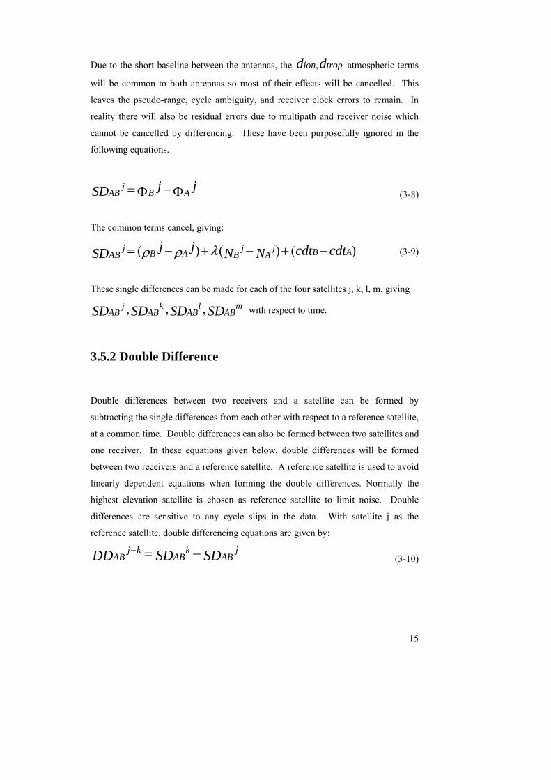
3.5.2 Double Difference

Double differences between two receivers and a satellite can be formed by

subtracting the single differences from each other with respect to a reference satellite,

at a common time. Double differences can also be formed between two satellites and

one receiver. In these equations given below, double differences will be formed

between two receivers and a reference satellite. A reference satellite is used to avoid

linearly dependent equations when forming the double differences. Normally the

highest elevation satellite is chosen as reference satellite to limit noise. Double

differences are sensitive to any cycle slips in the data. With satellite j as the

reference satellite, double differencing equations are given by:

ABj

ABk

ABkj SDSDDD −=−

(3-10)

16

With this the common receiver clock terms BA cdtcdt , cancel, leaving:

)()( Aj

Ak

Bj

BkA

jA

kB

jB

kAB

kj NNNNDD +−−++−−=− λρρρρ (3-11)

Repeating this for the remaining satellites gives three sets of double differenced

observations:

ABmj

ABlj

ABkj DDDDDD −−− ,, (3-12)

3.5.3 Triple Difference

Triple differences can be formed by differencing the double differenced data between

successive epochs. Doing this will cancel the common integer cycle ambiguity terms

since they will be the same over the observation period, provided there are no cycle

slips. Any carrier phase cycle slips will appear as outliers. The disadvantage of

triple differences is that they are sensitive to multipath, receiver noise and

atmospheric effects.

Triple differences can be formed between epoch’s t1 and t2 by:

)()( 12 tDDtDDTD ABkj

ABkj

ABkj −−− −= (3-13)

With this the common integer cycle ambiguity terms Aj

Ak

Bj

Bk NNNN ,,,

cancel, leaving:

)()()()(

)()()()(

1111

2222

tttt

ttttTDA

jA

kB

jB

k

Aj

Ak

Bj

Bk

ABkj

ρρρρ

ρρρρ

−++−

+−−=−

(3-14)

This procedure is done for the remaining satellites to give three sets of triple

differenced observations:

ABmj

ABlj

ABkj TDTDTD −−− ,, (3-15)

17

Chapter 4 GPS Receiver Development at QUT

The following chapter will briefly discuss the GPS receiver developments at QUT,

which formed the basis onto which the research presented in this thesis was

conducted [13].

In early 2002, Queensland University of Technology (QUT) commenced

development of its own GPS receiver (named the SPARx) with the capability for

space applications such as satellites in low earth orbits, and sounding rockets in a

way which is cost efficient. The QUT GPS receiver development is based on the

Zarlink (formerly Mitel) GP2000 Chip set and is a modification of the Mitel Orion

GPS receiver, which is a 12 channel receiver design [1]. The base for the software

development is the Mitel GPS Architect development kit [14]. The receiver is a

single frequency (L1) C/A code receiver.

4.1 SPARx Hardware

One outcome of this research was the procurement and manufacturing of three

SPARx GPS receivers in 2003. Each receiver consists of two boards, the lower

board being an interface board and the upper board which is the GPS receiver board.

These in the post production stage are shown in the pictures below (Figure 4-1,

Figure 4-2 and Figure 4-3).

18

Figure 4-1 SPARx Back View

Figure 4-2 SPARx Front View

Figure 4-3 SPARx Side View

19

4.1.1 SPARx Characteristics

The characteristics are listed below:

General L1 frequency (1575.42MHz), C/A code direct sequence spread-spectrum, 12 parallel channel continuous-tracking receiver

Signal Interface • Protocol RS232 • Data output ASCII strings

BAUD rate – 38400 bps 8 bits, no parity, 1 stop bit Approx. 3000 bytes of data per second

RF interface • GPS Antenna Active antenna configuration: 5 V

Power Requirements • Supply Voltage +8 to +30 volts DC • Current draw 600 mA • Power consumption 2 Watts

Environmental Characteristics • Operating Temperature -40 deg C to +85 deg C • Storage Temperature -50 deg C to +110 deg C

Connectors – on interface

board

• GPS RF SMA female • Antenna RF SMA male • Power 2.5 mm Power Socket • Signal DB9 male

Table 4-1 SPARx Characteristics

20

The core component of the receiver is the Mitel GP2000 Chipset. This includes the

GP2021 Correlator, ARM60-B RISC processor, DW9255 IF SAW filter and GP2010

RF Front End, as shown in Figure 4-4 and Figure 4-5. Consult references [1, 15] for

further information.

Figure 4-4 GPS Orion Architecture [1]

Figure 4-5 GPS Orion Receiver Block Diagram [15]

halla


halla


21

4.1.2 Temperature Compensated Crystal Oscillator

Figure 4-6 TXO200B Oscillator [16]

The SPARx uses the Rakon TXO200B 10.0 MHz temperature compensated crystal

oscillator for time reference, which has a standard specified frequency tolerance of

+/- 2 ppm over a temperature range of -30 to +70 deg Celsius. This is equivalent to a

time drift of +/- 2 μs/s. Figure 4-7 shows the frequency versus temperature

characteristic for the TXO200B oscillators used in the SPARx.

Figure 4-7 TXO200B Frequency Versus Temperature characteristic [17]

22

4.2 SPARx Software

4.2.1 Software Development and Test Environment

The GPS Architect development environment (Figure 4-8) is a 12-channel GPS

development system which can be used in hardware and software development

projects for embedded GPS receivers. Software for implementation into the SPARx

is written and compiled on a host PC and loaded via serial interface to the GPS

Architect for execution and testing. The GPS Architect is compatible to the Mitel

Orion design, which both use the Zarlink GP2000 chip-set.

Figure 4-8 Mitel GPS Architect Development Kit

4.2.2 Software Modifications

One outcome of this research is the latest SPARx software which is version 7.093.

This was based upon the previous version 7.07a which existed at the commencement

of this research.

Version 7.093 has the following additions and changes:

• Time synchronization capability, synchronized to UTC

• Integrated L1 carrier phase output in cycles

23

• Hardware pulse per second output aligned with the integer UTC second. A

more detailed explanation of the hardware pulse per second is given in 5.2.5.

• Introduction of non-volatile memory storage capability (storage of almanac

data etc)

• Modifications of receiver output format to accommodate the above

implementations

4.2.2.1 Operating System

The SPARx software uses a simple task switching operating system as used in the

GPS Architect and is based upon the structure shown in Figure 4-9. In the receiver

software version 7.093, modifications were made to the TNav and TTakeMeas tasks.

In addition, a new task named TPPS was added. The software interrupts were also

modified. Tasks can be suspended for a certain number of whole TICS (see 5.1.1)

and then re-activated. Refer to [18] for more information.

Figure 4-9 GPS Architect Software Structure [18]

halla


24

Chapter 5 Timing

The timing is one of the most critical aspects of a GPS receiver. Any inaccuracies in

the timing translate to inaccuracies in the measurements. These errors can then

incorporate inaccuracies in the resultant position and velocity information given by

the GPS receiver, especially in space where velocities in the kilometres per second

range are encountered.

The SPARx has an inexpensive reference clock which is a Temperature

Compensated Crystal Oscillator (TCXO), as given in 4.1.2. The frequency stability

of these types of clocks vary due to many factors. However, since SPARx is a

receiver for space applications, fluctuations in temperature and vibration are the main

contributing factors to frequency instability of its TCXO. Operations within the

receiver are dependant upon the stability and accuracy of this clock and the

receiver’s clock model.

As the broadcast GPS signal travels from the GPS satellite to the receiver, it will take

a certain time for it to travel. This time is the basis for the pseudo-range and carrier

phase measurements.

As can be seen in Figure 3-1 and Figure 3-2, any timing errors in the receiver’s time

will incorporate errors into the measurements, such as the code pseudo-range or

carrier phase measurements. This can have significant impact. If the receiver’s time

is inaccurate by 1 microsecond in a one second period of taking measurements, this

translates to sms /)103()101( 86 ××× − ~= 300 metres error in the pseudo-range

measurement. Likewise for the carrier phase, a 1 microsecond error in one second

means an error of approximately 1575.42 Hz.

For this reason precise measurement time intervals are required. This is particularly

important for the receiver to have carrier phase capability; otherwise there will be a

time error which results in an error in the carrier phase measurement. Software

improvements were made to align the timing in the SPARx with the integer second

25

of Coordinated Universal Time (UTC) so that precise time tagged measurements and

solutions may be obtained. Alignment with UTC was chosen because it is the

international time standard and is also the preferred time used in inertial navigation.

5.1 Timing in the SPARx

5.1.1 The TIC

The timing within the SPARx is derived from the oscillator (TCXO) - based ‘TIC’

which is an internal signal of the GP2021 correlator. It has a default period of

0.0999999 seconds. It is used to latch the measurement data of all 12 channels at the

same instant. The GP2021 correlator by Zarlink has the facility to let its default TIC

period of 0.0999999 seconds be modified in whole number increments of 175

nanoseconds which is the hardware (GP2021) time interval resolution [19].

5.1.2 Receiver Clock Model

Because the local clock in the receiver is a TCXO whose stability is much worse than

the atomic clocks onboard the GPS satellites, the receiver like most GPS receivers

has a clock model to relate the local clock to the GPS time.

The receiver software relates the oscillator based TICs to GPS time by counting

occurrences of the GP2021 TIC and then calculating the GPS time from the TIC

using a linear clock model. The clock model parameters (estimated receiver

oscillator bias and drift) are computed once every second as part of the navigation

solution if the receiver is tracking at least four GPS satellites. The receiver-modeled

GPS time is used to time tag the various raw measurements taken within the receiver,

which are then used in the navigation solution. If the broadcast UTC model

parameters are available then the measurements will be aligned with the receiver’s

own estimate of UTC time, which is derived from the calculated GPS time.

26

5.2 Time synchronization with the SPARx

Figure 5-1 Measurement Time Synchronization

As mentioned previously, for carrier phase navigation applications the time tag for

the measurements requires a precise measurement time. In the SPARx this was

achieved through software development and modifications. Software algorithms

were developed to synchronize the time when measurements are taken in the receiver

with the receiver’s own estimate of GPS time or UTC time. These improvements are

to ensure that the timing of the receiver is synchronized with GPS or UTC time and

that there is continual monitoring and adjustment to keep the synchronization. In the

current software implementation the GPS time will be used instead of the UTC if the

broadcast UTC model parameters are not available.

27

The time synchronization procedure implemented in SPARx is as follows:

1. If the receiver is tracking four or more GPS satellites, the receiver’s clock offset

(bias) and drift (both an output of the navigation solution) are used in the receiver

clock model to give an estimate of GPS time or UTC time.

2. The difference between the estimated GPS or UTC time and the estimated integer

GPS or UTC time is determined.

3. The TIC period is adjusted and the TNav task delayed so that it is aligned to the

receiver’s estimate of the GPS or UTC integer second.

4. The above procedures are repeated each second.

Two features of the GP2021 correlator [19] were utilized in order to align the time at

which measurements are taken and used in the navigation solution with the integer

UTC second. One feature is that the default TIC period of 0.0999999 seconds can be

modified. The other feature is that with the receiver’s operating system, the software

tasks (such as TNav) can be delayed by a certain number of whole TICs.

A new software task in the receiver code called ‘TPPS’ was designed and

implemented in the ANSI C programming language using the GPS Architect

development environment. This task performs the calculations required for the time

synchronization process.

28

5.2.1 Brief Description of TNav

The TNav task is the software task responsible for calculating a 3-dimensional

navigation solution, which includes the position and velocity of the receiver in the

Cartesian (x, y, z) WGS-84 Earth-Centred-Earth-Fixed (ECEF) coordinate frame,

and time information. This is done after processing the collected measurement data

which was collected at a certain time. This time at which the data is collected for

measurements is required to be aligned as close as possible to the integer UTC

second. The TNav task collects the measurements for a specific time, and then

calculates the relevant position, velocity, and time (clock model parameters)

information. The TNav task is activated at 1 Hz so each second there is the

possibility of a solution provided valid measurements from four or more tracked

satellites are available.

5.2.2 Alignment of TNav Task to Integer UTC Second

The time (TIC) at which the TNav task is activated was aligned to the integer UTC

second. Aligning the TIC at which the TNav task is activated, is effectively the same

as aligning the collection time of the measurements which are to be used in the

navigation solution. This is because the measurements within the receiver are taken

at a rate of 10 Hz (each TIC). This makes the assumption that when the TNav task

begins to process the measurements it will occur at the same time (TIC) as the time-

tag for the measurements itself, which is true in the current TNav software code. It is

assumed and has been observed that in the TNav task a time period of no greater than

0.0999999 seconds will elapse before the measurement data aligned to the integer

UTC second is used in the navigation solution.

5.2.3 The TPPS Task

The TPPS task calculates the delay required in suspending the TNav task by a certain

number of TICS, as well as the change in the default TIC period required. With the

29

current receiver operation the TPPS task is run only after a minimum of four GPS

satellites have been locked (Figure 5-2). This is done to ensure that the latest

receiver clock model parameters are available, thereby having a better approximation

of the GPS time within the receiver.

Figure 5-2 TPPS Activation

The TPPS task itself is designed to adjust its time of task suspension so that it

activates at two TICs behind the TIC at which the TNav task will be activated. This

is done to allow time for calculation of the TIC period change required, and a further

TIC period is required in which the default TIC period is modified in the hardware

[19]. This means that the TIC period in which the default TIC period is changed,

will be at the one TIC prior to when the TNav task activates. See Figure 5-3 below.

No

> 3 Sats ?

TNav

TPPS Start

Yes

30

Figure 5-3 TNav Alignment

The TPPS task calls a specific software routine which performs the required

calculations, as described in the following section.

5.2.3.1 Algorithm Design

1. When activated the TPPS task first takes a copy of the current TIC, and then

calculates the current UTC (or GPS time if UTC is not available) second from

this TIC.

Example:

The current TIC is number 1253, which the receiver clock model calculates to be at

25.6785 seconds UTC.

TNav, aligned as close as possible to integer UTC second

TIC period change required is calculated

TPPS

TIC period changed

TICS

31

Figure 5-4 TPPS Example 1

2. The software then calculates the time away from the next integer 10th of the

UTC Second.

Example:

The next integer 10th of second is 0.7 seconds, time difference = 0.7 – 0.6785 =

0.0215 seconds (see Figure 5-5 to Figure 5-7).

Because 0.6785 is close to 0.7 seconds, it is better to change the TIC period by

increasing the default value rather than shortening it. It is increased by 0.1 seconds

to bring the TNav task to align to the integer 10th of UTC which will be at 0.9

seconds.

Therefore the new TIC period is 0.0215 + 0.1 seconds = 0.1215 seconds.


PPS Task start

25.8784998

TNav 1 Task start TIC 1253

25.6785000 seconds

0.0999999 s

1254 1255

25.7784999

PPS Task start TNav 1 Task start TIC 1253

25.6785000 seconds

25.8784998

0.0999999 s

1254 1255

25.7784999

32



3. Because the calculations to correct the TIC were performed at the one TIC

prior to the TIC in which the actual TIC period has changed, the software

corrects this value by 100 nanoseconds which is the time error between the

default TIC period of 0.0999999 and 0.1 seconds (see 5.2.4.3).

Example:

The new TIC period required is then 0.1215 + 100 ns = 0.1215001 seconds.

4. This value is then converted into the various registers required and resolution

that can be achieved with the GP2021 and it is this value that the hardware

TNav 1 Task start

25.6785

25.9 25.7784999

0.1215 seconds

PPS Task start TIC 1253

25.7 seconds

0.0999999 s

1254 1255

25.6785

TNav 1 Task start

25.8784998 25.7784999

PPS Task start TIC 1253

25.7 seconds

0.0999999 s

1254 1255

33

can achieve (a multiple of 175 nanoseconds) that will be the actual new TIC

period.

Example:

The actual TIC period that can be achieved with the GP2021 time interval resolution

of 175 nanoseconds = 0.12150005 seconds (Figure 5-8). For this point the relative

error introduced due to hardware limitation is therefore 50 nanoseconds, which is

discussed further below in 5.2.4.1.


5. After the alignment is made of the TNav task to the integer tenth of a UTC

second, the final step of aligning the TNav task to the integer UTC second is

performed. This is achieved by delaying the TNav task itself by a whole

number of TICs, which will effectively line up the next TNav task to be at the

integer UTC second.

Example:

In the example given above, the TNav task is aligned to 25.89999995 seconds. The

next TNav task, with a task suspension interval of 10 TICS (navigation solution

output is at 1 Hz), will be at 26.9 seconds. This means that delaying the TNav task

by 1 TIC period is required. The next TNav task will then be at 27.0 which is the

TNav task aligned to the integer UTC second (Figure 5-9).

25.6785

25.89999995

TNav 1 Task start

25.7784999

PPS Task start

0.12150005 s 1254 TIC 1253

25.7 seconds

0.0999999 s

1255

34


After the actual TIC period is changed in the GP2021 hardware, the change in the

default TIC period is reflected in the software by correcting the receiver clock model

with the time modifications.

To avoid a delay in the TNav task, the software also accounts for certain cases where

the adjustment to align the TNav task to the integer UTC second falls between 0.17

to 0.45 seconds away from the next integer UTC second. These values were chosen

as the minimum and maximum TIC periods that can be reliably achieved in the

hardware to allow adequate time for processing the software commands. In this case

the TIC period is adjusted between these values accordingly so no delay to the TNav

task will be required.

6 11 10

11 TIC delay

27.0

TNav 1

TNav at integer UTC second

25.9 s 26.9 26.0 26.1 26.2

1 2 3 4 5 7 8 9

TNav 2

35

5.2.4 Time Synchronization Issues

The following sections address the most common error sources and limitations in the

time synchronization process with the SPARx.

5.2.4.1 TIC Interval Resolution

As given in 5.1.1 the TIC interval resolution is limited to 175 nanoseconds, which is

not a sub-multiple of 1 second. This contributes to the main error source in the TIC

alignment process in the software. Though the hardware is limited to the resolution

of 175 nanoseconds, the observed error between what was desired and what could be

achieved due to hardware limitations was in the magnitude of about 50 nanoseconds.

The clock resolution can be calculated as 5.5012/175 = nanoseconds [20], which

is what was observed. This is the standard deviation of a uniformly distributed error

ranging over 175 nanoseconds. The time synchronization algorithm is designed so

that the absolute error of this should always be less than 87.5 nanoseconds, as it will

be aligned to the nearest multiple of 175 nanoseconds.

5.2.4.2 Oscillator Error

The physical oscillator accuracy and stability varies with temperature and vibration.

As given in 4.1.2 the Rakon TCXO has a specified frequency of +/- 2 ppm over its

operating temperature range. This means there could be up to +/- 2 ppm variation on

the TIC which is equivalent to +/- 200 nanoseconds variation per TIC.

The receiver clock model compensates for most of the error from the oscillator by

using the estimated oscillator bias and drift which is calculated each second in the

navigation solution. However there is still some residual error due to any

36

temperature or vibration changes between estimates of the receiver clock model

parameters.

In the time synchronization algorithm, the alignment to the TNav task was performed

as close as possible to the TNav task activation TIC (at the TIC prior to the TNav).

This was to minimize the effect of the oscillator residual error on the calculations

(see Figure 5-3).

5.2.4.3 Default TIC Period

The TIC period of 0.0999999 seconds is not a sub-multiple of 1 second so a ‘1

second’ period in the original software is not 1 second but 10 TICS which is

0.999999 seconds. This is 1 micro second away from a true 1 second period.

This is corrected for in the time synchronization algorithm as given in 5.2.3.1

5.2.4.4 UTC Time Transfer Error

There will be an introduced error associated with aligning to UTC, estimated by [12]:

Error Range TDOP × (5-1)

TDOP is the Time Dilution of Precision which is the contribution of clock error to

the error in pseudo-range. It can be calculated from the navigation solution in the

receiver.

The range error can be estimated by the user range accuracy (URA). The URA is the

Master Control Station’s prediction of the pseudo-range accuracy obtainable from a

GPS satellite’s signal. It is transmitted in the navigation message for each satellite.

37

5.2.5 Hardware Pulse Per Second

A hardware pulse per second (PPS) was generated out of the GP2021 correlator,

aligned with the UTC integer second. It is output if four or more GPS satellites are

tracked. It is a 1 ms wide pulse output on DISCIO pin 32 of the GP2021 correlator

[19] at a frequency of 1 Hz. It may be used as a time reference for operations and

measurements and to synchronize the sub-systems onboard a satellite, for example.

Figure 5-10 is a picture of the PPS rising edge.

Figure 5-10 SPARx PPS

5.2.5.1 SPARx Hardware Pulse Per Second Time Error Budget

Various factors influence the accuracy of the SPARx hardware pulse per second to

the integer UTC second. These can be separated into two parts, the random error and

the bias. These are listed and estimated as follows:

38

1. The Time Transfer Error from GPS Satellites to User

Reference [8] states that standard positioning service receivers can achieve

approximately 337 nanosecond (95%) UTC time transfer accuracy. This

value includes error introduced by selective availability (SA), which is

currently turned off since the year 2000. Without SA, a more typical value of

time transfer error can be estimated. Using equation (5-1) with a typical

value of TDOP of 1.5 and range error of 6 metres, gives a time transfer error

of 9 metres. Converting this to time gives approximately 30 nanoseconds

time transfer error [12].

2. TCXO Instability Error

The TCXO varies with temperature and vibration (see 5.2.4.2).

This can be estimated from the TCXO data sheet such as [16].

Assuming a maximum temperature variation of 2 deg C / min and the

maximum change is 2 ppm /deg C. In a one second period, the error will be 2

deg C/min × 2 ppm/deg C = 33 nanoseconds.

A typical value for oscillator drift error is 20 ns [20].

3. Receiver Clock Resolution

The TIC resolution limitation is 175 nanoseconds, which means a clock

resolution of 50.5 ns as given in 5.2.4.1.

The total RMS = RMS of (Time Transfer Error + Oscillator Drift Residual

Error + Clock Resolution)

The root mean square is calculated according to [21]:

∑=

=n

iix

nRMS

1

21 (5-2)

Total RMS 3

5.502030 222 ++= = 35.8 ns

39

Estimated Total Random Error

Delay Value

Time transfer 30 ns

TCXO error 20 ns

Clock resolution 50.5 ns

TOTAL (RMS) 35.8 ns (RMS)

Table 5-1 Estimated Total Random Error

4. The Bias

The PPS will have a bias from the integer UTC second due to delays

associated with the hardware. This is the main error source. The GP2021

correlator, GP2015 front end and ARM60-B processor are the main

contributors to this bias.

The documented delays specified for the GP2021 are found in the GP2021

manual [19] and are listed below in Table 5-2:

GP2021 Estimated Total Bias

Delay Value

Timemark generation 150 ns

Bus Interface delay 300 ns

Processor write operation 350 ns

Digital signal path delay 400 ns

TOTAL 1200 ns

Table 5-2 GP2021 Estimated Total Bias

The estimated total delay due to the correlator alone in the hardware pulse per

second is therefore 1200 ns.

40

Chapter 6 Carrier Phase Processing

6.1 GPS Receivers and Carrier Phase

The use of carrier phase in GPS for navigation is important for precise positioning

applications and has been used in fields such as precise navigation and surveying for

many years. The advantage of using carrier phase instead of the code pseudo-range

information alone in a receiver is that the carrier phase wavelength on the L1

frequency (1575.42 MHz) is only approximately 0.19 metres. This is much smaller

than the C/A code chip length which is about 293 metres. Likewise, the precision of

the carrier phase measurements is in the millimeter range (2mm with the GP2021,

see 6.3.1) while the code range measurement’s precision is at the metre level. Using

the carrier phase means that very precise point positioning and relative positioning

solutions may be obtained. The disadvantage of using the carrier phase is that it is a

relative measurement so absolute range measurements can not be made using the

carrier phase directly, unless the integer cycle ambiguity can be determined.

Two carrier signals in the L-band, named L1 and L2, are generated by integer

multiplications of the fundamental frequency which is at 10.23 MHz. The L1 carrier

frequency is 1575.42 MHz and the L2 carrier frequency is 1227.6 MHz.

41

6.2 Carrier Phase Measurements and Applications

The following sections briefly describe the use of carrier phase in various

applications, such as absolute positioning, relative positioning, and attitude

determination. Hofmann-Wellenhof et al. [9] contains more detailed explanation of

the following.

6.2.1 Absolute Positioning

Absolute positioning (otherwise known as point positioning) is determining the

location of an unknown point with respect to a common known reference frame, such

as the WGS-84 Earth-Centred-Earth-Fixed (ECEF) coordinate frame. The unknown

position can be determined using a single receiver and can be stationary (static) or

moving (kinematic).

Absolute positioning with code pseudo-ranges only requires at least four pseudo-

range observables to solve the four unknowns (x, y, z coordinates and the time) for

the receiver. This is attractive because a solution can be obtained based on

measurements for a single epoch, however the accuracies that can be obtained are

poorer than those that can be obtained from relative positioning.

Pseudo-ranges obtained from carrier phase measurements are not normally used in

absolute positioning. This is because multiple epochs are required and the position

accuracy that can be obtained is poorer than can be obtained in relative positioning.

Even so, it is a possibility to use the carrier phase for absolute positioning. Using

carrier phase measurements incorporates additional unknowns, the integer cycle

ambiguities. Integer cycle ambiguity resolution is therefore a necessary part of the

process. Additional measurements from multiple epochs are required to be able to

solve the additional unknowns. In all cases the number of observations must be

equal to or greater than the number of unknowns to be able to obtain a solution.

Obtaining a solution is dependant upon the number of observations required, which

depends upon the number of satellites in view and the number of epochs over which

42

the observations can be made. According to the relationship given in Hofmann-

Wellenhof [9], the total number of observations is tjnn where jn is the number of

satellites and tn is the number of epochs. For static point positioning with carrier

phase measurements, the number of observation epochs required is given by [9]:

13

−

+≥

j

jt n

nn (6-1)

For example, according to equation (6-1), if the number of satellites in view is 5 then

the minimum number of epochs required to be able to solve the unknowns is 2.

For kinematic point positioning with carrier phase measurements, the number of

observation epochs required is given by [9]:

4−=

j

jt n

nn (6-2)


the number of epochs required to be able to solve the unknowns is 5.

As can be seen, the time required to obtain a solution depends on the number of

measurements used and the number of unknowns to solve. Solutions for a single

epoch are not possible for point positioning with carrier phases, unless the jn integer

ambiguities are known from initialization. The integer cycle ambiguity will be

constant over time provided there are no cycle slips. Due to the risk of cycle slips in

using multiple epochs, a disadvantage of using carrier phase in point positioning is

that it is not stable or robust unless it is monitored closely. Monitoring by cycle slip

detection and correction is therefore necessary to ensure robustness and accuracy.

For this reason carrier phase measurements are normally used in relative rather than

absolute positioning.

43

6.2.1.1 Carrier Phase Smoothed Pseudo-ranges

The carrier phase can be used to smooth the code pseudo-ranges. By doing so this

combines the absolute and noisy code pseudo-ranges with the ambiguous (due to the

integer cycle ambiguity) but highly accurate carrier phase. This procedure can be

employed by carrier phase capable GPS receivers and is also important for real-time

trajectory determination [9].

6.2.2 Relative Positioning

The use of carrier phase in differential GPS, commonly known as CDGPS, can

provide a very precise position solution. Relative positioning (otherwise known as

differential positioning) is determining the coordinates of an unknown location with

respect to a known location. In this case two or more receivers are used. Refer to

Figure 3-4.

The receiver at either location can be stationary or kinematic. The receiver at the

known location (master) can transmit differential corrections (e.g. via VHF link) to

the receiver at the unknown location (slave). Otherwise the data from both receivers

can be post processed after the observation session. Single differenced and double

differenced observables can be formed and these contain the integer ambiguity that

needs to be determined. Triple differences however do not contain the unknown

integer ambiguity due to the canceling process. Triple differences are not normally

used since the position solutions obtained tend to be less accurate than from double

differences [12].

Double differences are the most preferably used observables in relative positioning

due to the canceling of the clock errors. According to the relationship given in

Hofmann-Wellenhof [9], the number of observations is tjnn where jn is the

number of satellites and tn is the number of epochs. For static relative positioning

with double differenced carrier phase measurements, the number of observation

epochs required is given by [9]:

44

12

−

+≥

j

jt n

nn (6-3)


the minimum number of epochs required to be able to solve the unknowns is 2.

For kinematic relative positioning with double differenced carrier phase

measurements, the number of observation epochs required is given by [9]:

41

−

−=

j

jt n

nn (6-4)

For example, according to equation (6-4), the minimum number of satellites in view

required is 5. Therefore the number of epochs required to be able to solve the

unknowns is 4.

For navigation, the unknown position must normally be determined in a single epoch

due to the changes in position. This is known as real-time kinematic positioning. It

can be seen by the above examples that it is impossible to calculate a solution in one

epoch without knowing the cycle ambiguities. The ambiguities to be determined

must be known beforehand or calculated within the single epoch otherwise the set of

equations will be underdetermined and therefore unsolvable. The concept of real-

time kinematic differential positioning can be employed in many different

applications. Such applications include precision landings for aircraft, onboard

relative navigation between two or more satellites formation flying in space, or a

multi-antenna GPS receiver for 3-axis attitude determination using the

interferometric principle as discussed in 6.2.4.

6.2.3 Cycle Ambiguity Resolution

For SPARx to be used in relative navigation and attitude determination, ambiguity

resolution is required to be calculated in real time, within a single epoch. This is

commonly known as ‘on-the-fly’ ambiguity resolution and is the most challenging

45

since it requires the ambiguities to be determined near instantaneously in a moving

receiver. As mentioned in the previous section, the ambiguities must be known

before a navigation or attitude solution can be calculated in one epoch. A solution in

one epoch is not possible otherwise. The correct integer cycle ambiguities need to be

estimated and the position or attitude can then be determined for the moving receiver

in the subsequent epochs. This is providing there are no cycle slips and the

minimum required number of GPS satellites is available.

Cycle ambiguity resolution procedure will be briefly discussed here relating to the

real-time kinematic case. There are a few algorithms that have been developed that

can solve the ambiguity in a single epoch, such as the least squares ambiguity search

technique by Hatch [9, 22, 23]. There are a couple of methods existing of the least

squares ambiguity search technique and one is given below as an example of its use

in relative navigation. The procedure given is from Hatch [22]. The least squares

ambiguity search technique can also be used in attitude determination given the

constraint that the baseline length is known and fixed, thereby reducing the search

space.

The procedure is as follows:

1. Estimate the initial position

An initial estimate of user position is made from a code pseudo-range

differential solution for example.

2. Use a search algorithm to identify likely integer combinations and choose the

best set of integer combinations.

The least squares ambiguity search technique involves choosing four

satellites in view which have the best user-satellite geometry. These are

called the primary group. While double differences are not used in this

method, carrier phase differences are then formed between three of the

satellites and a reference satellite to eliminate receiver clock bias. Any

redundant satellites in view are used as a secondary group of satellites. The

46

primary group of satellites and carrier phase is used in constructing a search

space around the approximate location of the unknown receiver antenna. A

number of potential solutions are then obtained. The secondary group of

satellites is used to eliminate incorrect potential solutions. This is done

through least squares adjustment, where the minimum sum of squared

residuals can be used to identify incorrect potential solutions. Ideally only

the true solution should remain after identifying all the incorrect potential

solutions. If this is not the case then the solution with the smallest sum of

squared residuals should be chosen.

Identifying one true solution depends upon the noise level of the carrier phase

measurements and the number of satellites available. The noise level of the

measurements is very important in identifying one true solution. If the carrier

phase measurement noise is less than +/- 4.75 mm, each redundant satellite

can reduce the number of potential solutions included in the search region by

5%. If more satellites are available it means that the number of potential

solutions in the search region can be reduced. This increases the probability

of identifying one true solution and reduces the amount of time to do so.

Based on tests made by Hatch [22], there are three conditions that if met, will

normally mean the ambiguities can be resolved in a single epoch:

(1) Dual frequencies are available for a technique called ‘wide-laning’ to be

used.

(2) Baselines are less than a few tens of kilometers, so that ionospheric errors

are minimal.

(3) There are 7 or more total satellites available for tracking.

The least squares ambiguity search technique can be used with single or dual

frequency measurements. By using a single frequency receiver it will

generally take 4.5 times longer to resolve the ambiguities than with a dual

frequency receiver. The use of a single frequency receiver can be made up

for by having one additional satellite available [22].

47

3. Calculate the final solution with the new fixed ambiguities.

The final solution is calculated with the new fixed ambiguities. The known

ambiguities can be used in double differenced carrier phase measurements to

achieve a very precise position solution. Cycle slip detection and correction

will be required to detect and correct any changes in the cycle ambiguity to

ensure continuous navigation. Whenever the number of satellites has

temporarily dropped below the minimum of four, the least squares ambiguity

search procedure can be made to re-calculate the cycle ambiguities.

6.2.4 Carrier Phase and Attitude Determination

Attitude determination is one specific application of using the carrier phase in

relative measurements. 3-axis attitude determination is defined as determining the 3-

axis orientation of a body fixed system with respect to a reference system. The

objective being to determine the parameters of pitch, roll and yaw. Such information

is required for satellites whose attitude control system ensures that the satellite and

payloads are facing in the right direction. On satellites this is especially important

for any solar panels, communications equipment, cameras and other devices where

orientation is a key factor in the quality of their data or use. It is often necessary to

have accurate and reliable attitude information for such reasons.

The advantage of using GPS for attitude determination is that it is a low cost

alternative to other techniques using gyroscopes or star sensor instruments [24]. It

may also provide benefits in terms of lower power and lower weight to the other

devices. There have been experiments from past projects that show that a GPS

receiver with multiple antennas can be successfully used for attitude determination

[5]. One such experiment was RADCAL launched in June 1993 which was the first

spacecraft where attitude determination with GPS was tested in space [25-27].

48

6.2.4.1 Multi Antenna GPS Receiver

If a GPS receiver is modified for multiple antennas separated by fixed baselines,

relative measurements can be made using the carrier phase of the GPS signal. Chu

and Woerkom [25] explains how the observable for GPS attitude determination is the

difference in carrier phase between a master antenna and one or more slave antennas.

A minimum of three antennas are required to measure 3-axis attitude or four

antennas can be used for redundancy [24]. The accuracy of such a system is

influenced by multipath, baseline lengths and the calibration of the line bias.

Multipath is dependant on the spacecraft design, and increased baseline lengths result

in improved angular accuracy [9]. It is stated that such a system can provide

accuracy better than 0.2 degrees [24]. This carrier phase difference measuring is the

most commonly used method since it provides the high measurement accuracy

required for attitude determination. A disadvantage of using this method is that the

integer ambiguities need to be resolved [25]. This requires the use of integer

ambiguity resolution algorithms such as presented by C. Arbinger et al. [28], S. Yoon

et al. [29] and J.C. Juang [30].

The following diagram shows the interferometric principle, which forms the basis for

the carrier phase difference measuring. The large distance between the GPS

satellites and GPS receiver means that the incoming signals appear parallel at the

antenna. By differencing the signal between both antennas, determining λN + Δφ

and with the baseline AB known, the angle γ can then be determined mathematically.

49

Figure 6-1 Interferometry using GPS

It is assumed that the signals appear parallel at the antennas due to the large distance

between the antennas and GPS satellites.

The difference of the slant range is given by [28]:

φλρ Δ+=Δ N (6-5)

λ is the L1 carrier phase wavelength.

N is the whole cycle (integer) ambiguity (unknown and has to be determined).

Δφ is the fractional L1 wavelength.

The difference of the slant range can be obtained by the scalar multiplication of two

vectors:

busB ⋅=Δρ (6-6)

Δρ = λN + Δφ Δφ

γ

Antenna B

GPS Satellite

Antenna A

sBu

b

λN

50

6.3 Carrier Phase with the Zarlink GP2021

6.3.1 Implementation of Carrier Phase in SPARx

The Orion reference design does not have carrier phase implemented by default.

Therefore the SPARx software was modified to output the integrated carrier phase in

L1 cycles. One feature of the GP2021 correlator is that the integrated carrier phase

can be measured, with a resolution of 10-bits to give 1024/2π radian increments.

This corresponds to a resolution of approximately 2 mm on the carrier phase [19].

This is achieved by measurement of the integrated carrier phase through the

CHx_CARRIER_CYCLE_HIGH, CHx_CARRIER_CYCLE_LOW and

CHx_CARRIER_DCO_PHASE registers, which are part of the measurement data

sampled every TIC period [19].

The GP2021 employs a DCO (Digitally Controlled Oscillator) for the carrier

generation where the nominal DCO phase advance over 1 TIC interval is given as

-140539.542 cycles/TIC [14].

In the receiver software the carrier phase measurement is given by:

cyclesDCOfnomT _−×Δ=ΔΦ (6-7)

Where:

ΔΦ is the phase change (in cycles) over TΔ , cyclesDCO _ is the carrier DCO cycle

count over TΔ and fnom is the nominal carrier DCO frequency.

The nominal carrier DCO frequency with no Doppler and no oscillator drift

compensation is 1.405396825 MHz. In 100 ms for example, there will be 140540

cycles [19], therefore:

51

Tfnom Δ××= 6104053926825.1 [Hz] (6-8)

The number of carrier DCO cycles, cyclesDCO _ , is obtained by reading the

CHx_CARRIER_CYCLE_HIGH and CHx_CARRIER_CYCLE_LOW registers of

the GP2021 at every TIC and summing the readings. This gives a number which is 1

cycle higher than the number of complete carrier cycles. To this number the

fractional carrier cycle at the last TIC has to be added, and the fractional carrier cycle

at the beginning has to be subtracted, as shown in Figure 6-2.

The phase change can then be calculated at each TIC, and summed over 10 TICS to

give the total carrier phase change in one second [19]:

At each TIC:

1024/)______(___

phaseDCOcarrierinitialphaseDCOcarrierfinalcountercyclecarriercyclesDCO

−+=

(6-9)

Equivalent equations are given below in the following diagram Figure 6-2.

For each tracked GPS satellite the total phase change over one second is obtained.

This is added to the total number of phase changes since signal lock-on to give the

integrated carrier phase measurement.

52

Figure 6-2 Carrier Phase [19]

6.3.2 Carrier Tracking Loop

The receiver has a carrier tracking loop implemented which is a second-order

frequency lock-loop (FLL) with a bandwidth of 1 Hz, as described in [31]. As given

in [14] the FLL offers good dynamic performance, robustness and insensitivity to

interference.

To improve the carrier phase tracking performance in the SPARx, the existing FLL

bandwidth was narrowed. This showed some improvement in the carrier phase

resolution but no real advantage to the currently selected bandwidth. Kaplan [32]

describes various types of loop filters, one of which could be suitable for

implementation into the SPARx to improve the carrier phase tracking performance.

The following picture is of a third-order phase lock-loop (PLL) filter with second-

order FLL assist from [32]. It can operate in a combination PLL/FLL mode or either

a pure FLL or PLL, depending on the input. The PLL is more accurate than the FLL

but is more sensitive to dynamic stress. Dynamic stresses in the loop can cause the

halla


53

PLL tracking loop to lose lock. The dynamic stress is dependent on signal dynamics

and the bandwidth of the loop. High receiver dynamics produce high dynamic stress

in the tracking loop. Therefore the concept is to have the 2nd order FLL cope with

the dynamic stresses while the 3rd order PLL gives better accuracy. Overall this

should result in good tracking performance in both a dynamic and static

environment.

Figure 6-3 Third-order PLL with second-order FLL assist [32]

After initial investigation, implementation and testing of the above third-order PLL

with second-order FLL assist in the SPARx, it was found that the main factor

affecting the implementation of such a loop filter is the remaining processor power

within the receiver. Since the receiver is modified in software for space applications

the remaining processing power of the receiver is limited. Efficient ANSI-C coding

in the receiver software is required to be able to implement this filter but at the

expense of introduced errors in the filter parameters from the ideal values given in

[32]. Bandwidths and loop filter parameters therefore need to be chosen with the

restriction in processing power of the SPARx in mind.

halla


54

Chapter 7 Tests and Results

Tests were conducted as described in the following sections to evaluate the receiver

software modifications.

7.1 Test Equipment

7.1.1 GPS Signal Repeater

There is a repeater which broadcasts re-radiated GPS signals indoors into the

laboratory from an antenna on S block roof at QUT. This allows the GPS receiver to

be used indoors.

Figure 7-1 GPS Signal Repeater

7.1.2 Software Development and Test Environment

The following is the SPARx software development and testing environment with the

Mitel GPS Architect. Software can be uploaded to the Architect for execution from

the computer.

55

Figure 7-2 Software Development and testing with the GPS Architect

7.1.3 GPS Signal Simulator

A six channel L1 C/A code GPS signal simulator (Welnavigate GS720) was

available for testing the GPS receiver software under various static and dynamic

scenarios (such as on a Low Earth Orbiting satellite).

Figure 7-3 Welnavigate GPS Signal Simulator

56

7.2 Timing Tests

7.2.1 SPARx Measurement Time Tag Tests

The following comparisons were made to check the relative accuracy of the

measurement time tags and the implementation of the time synchronization

algorithm in the SPARx. This comparison was made with respect to the receiver’s

own estimate of UTC time which is derived from the receiver’s clock model. The

time at which the measurements are taken and used in calculating a navigation

solution in the TNAV task were recorded and output via the GPS receiver serial port.

The receiver was operated in a static environment outdoors on the top of QUT S

block roof.

7.2.1.1 Results

A set of data for the receiver running over a period of 13.6 hours is shown below in

Figure 7-4. The vertical axis shows the offset between the time tag of the

measurements and the receiver’s estimate of the integer UTC second. The horizontal

axis is the receiver’s own estimate of the UTC integer second. Figure 7-5 shows the

number of tracked satellites by the receiver, for the same time period as Figure 7-4.

By comparing Figure 7-4 with Figure 7-5 it can be seen that most of the jumps in the

data in Figure 7-4 is where the receiver loses time synchronization. This is due to

there being less than four satellites tracked by the receiver at those times. It can be

seen in Figure 7-4 that the time synchronization algorithm reacquires

synchronization again after four or more satellites are locked.

57

Figure 7-4 Time Synchronization 1

Figure 7-5 Satellite Acquisition

58

The following data plot is a closer look at an 83 minute period section of the data

shown in Figure 7-4.


This data has a mean of 66.8 ns nanoseconds with standard deviation (1 sigma) of

50.6 nanoseconds. The spread of the data is 178 nanoseconds.

Figure 7-7 is a plot of another section of the data shown in Figure 7-4 for a 100

seconds period, where the mean of the data is much less than the mean shown in

Figure 7-6.

59


This data has a mean of 2.08 nanoseconds with standard deviation (1 sigma) of 50.64

nanoseconds. The spread of the data is 174.6 nanoseconds.

7.2.1.2 Conclusions

Figure 7-4 shows that after losing synchronization the software successfully realigns

the time again.

Figure 7-6 and Figure 7-7 show that the timing of the SPARx is aligned with respect

to the receiver’s own calculation of the integer UTC second.

For both sets of data statistics given for Figure 7-6 and Figure 7-7:

The standard deviations shown are consistent with the clock resolution of 50.5

nanoseconds as given in 5.2.4.1.

60

The spreads of the data of approximately 175 nanoseconds are consistent with the

TIC interval resolution of 175 nanoseconds.

The means of the data show that a mean of 2 nanoseconds can be achieved, with

other values around 66 nanoseconds. These values are within the maximum

expected error of 87.5 nanoseconds as stated in 5.2.4.1.

7.2.2 Hardware PPS Test

This test was performed to check the accuracy of the SPARx hardware pulse per

second (PPS) (see 5.2.5) with respect to the integer UTC second. Measurements

were made between the hardware PPS from the SPARx with the hardware PPS from

an Ashtech μZ-CGRS (micro-Z, Continuous Geodetic Reference Station). The

receivers were stationary and run over a four hour period with both continuously

outputting a pulse every second. Samples of the pulses were taken at random times

and the offset between them measured using an Agilent 54621A Oscilloscope. The

PPS of the Ashtech receiver is documented to be synchronized within 1 microsecond

of GPS time [33]. The Ashtech receiver was using a Symmetricom 4065C Cesium

frequency and time standard (atomic clock) for a stable reference oscillator. The

atomic clock also outputs a hardware PPS which was also used for comparisons.

This atomic clock’s PPS was not synchronized to UTC time or GPS system time.

Firstly, measurements of the time offset between the hardware pulse per second

(PPS) outputs of the SPARx and the atomic clock were taken. These are shown in

7.2.2.1. Then measurements of the time offset between the PPS of the Ashtech

receiver and the atomic clock were made, given in 7.2.2.2. Then the comparisons

were made between the Ashtech μZ-CGRS and the SPARx hardware PPS with the

results given in 7.2.2.3.

61

The test setups are shown in the following diagrams:

Figure 7-8 Atomic Clock and SPARx PPS Test Setup

Figure 7-9 SPARx and Ashtech PPS Test Setup

Oscilloscope

SPARx Ashtech μZ

PPS Output PPS Output

Probe Lead 2m

0.4 m Test Lead0.2 m Test Lead

Oscilloscope

SPARx

4065C Cesium Clock

PPS Output

PPS Output

Probes – equal type & length

1 metre, 50 Ohm Coax Cable

0.2 m Test Lead

62

7.2.2.1 Results – Atomic Clock and SPARx

This figure shows an atomic clock pulse and a SPARx pulse as indicated by the

arrows. Using the oscilloscope the offset between the rising edges of these two

pulses was measured as 449.687 ms.

Figure 7-10 Atomic Clock and SPARx PPS

7.2.2.2 Results – Atomic Clock and Ashtech

This figure shows an atomic clock pulse and an Ashtech receiver pulse as indicated

by the arrows. Using the oscilloscope the offset between the rising edges of these

two pulses was 448.687 ms.

Atomic Clock PPS

SPARx PPS (inverted)

63

Figure 7-11 Atomic Clock and Ashtech PPS

The time offset between a pulse of the atomic clock and SPARx and atomic clock

and Ashtech was measured again approximately 2 hours later. The difference

between the clock and SPARx pulses and clock and Ashtech pulses was 449.690 ms

and 448.688 ms respectively. The results are listed in the table below, along with the

difference between these two results which is the difference between the SPARx and

Ashtech pulses:

Sample

Clock and

SPARx PPS

Time Offset

Clock and

Ashtech PPS

Time Offset

Calculated

difference

between

SPARx and

Ashtech Time

Offsets

First sample 449.687 ms 448.687 ms 1 ms

~ 2 hours

later

449.690 ms 448.688 ms 1.002 ms

Table 7-1 Atomic Clock and Receiver PPS Results

Atomic Clock PPS

Ashtech PPS (inverted)

64

7.2.2.3 Results - SPARx and Ashtech

Figure 7-12 below shows an Ashtech receiver pulse (inverted for easier visualization)

and a SPARx pulse as indicated by the arrows. The offset which was measured is

also indicated on the figure. Because these two pulses are close together a finer

resolution (500 μs/div) than Figure 7-11 could be used to view the two pulses on the

oscilloscope as shown below.

Figure 7-12 SPARx and Ashtech PPS

Over a three hour period, one set of pulses (one SPARx pulse, one Ashtech pulse)

were selected at random times and the offset between them was measured.

Sometimes two consecutive sets of pulses were measured, to see if there is much

variation between consecutive seconds. The results of this procedure are listed in

Table 7-2. As indicated in Table 7-2, during the test the SPARx PPS

synchronization was lost due to less than four GPS satellites being tracked by the

receiver. Synchronization was re-gained after 15 minutes.

The time offset between the pulses was measured at the following locations on the

leading edges (as indicated by the vertical dotted line):

SPARx PPS Leading Edge

Ashtech PPS (inverted) Leading Edge Offset

65

Figure 7-13 Ashtech PPS Leading Edge (inverted)

Figure 7-14 SPARx PPS Leading Edge

66

Sample Time SPARx and Ashtech

Time PPS Offset

SPARx and Ashtech

PPS Time Offset (next

second)

1 First sample 1.00198 ms

2 ~ 30 min later 1.00200 ms

3 ~ 6 min later 1.00200 ms

4 ~ 2 min later 1.00200 ms

5 ~ 2 min later 1.00300 ms

6 ~ 2 min later 1.00198 ms 1.00198 ms

7 ~ 15 min later 1.00300 ms

8 ~ 0.5 min later 1.00300 ms

9 ~ 1 min later 1.00200 ms

10 ~ 1 min later 1.00202 ms

PPS synchronization lost (less than 4 Satellites locked)

11 ~ 15 min later 1.00200 ms

12 ~ 120 min later 1.00400 ms

13 ~ 1 min later 1.00400 ms 1.00400 ms

14 ~ 1 min later 1.00200 ms 1.00198 ms

Average 1.00250 ms

Table 7-2 SPARx and Ashtech Receiver PPS Results

7.2.2.4 Conclusions

The atomic clock’s pulse was known to be unsynchronized to GPS or UTC time.

The comparison between the SPARx and Ashtech pulses with the atomic clock pulse

of 449.687 ms and 489.687 ms (given in Table 7-1) confirms that the atomic clock’s

pulse is not synchronized to GPS or UTC time.

With Table 7-2, the consecutive samples that were measured of between the SPARx

and Ashtech pulses shows that the variation is not too large between those seconds

(samples 6, 13 and 14). The variation is of approximately 20 nanoseconds for

sample 14 (as best could be read from the oscilloscope).

67

It can also be seen that there is not much variation (20 nanoseconds) between

samples 10 and 11 after losing synchronization for 15 minutes and then regaining

synchronization.

Over the sample period the minimum offset measured was 1.00198 ms and the

largest was 1.00400 ms. A 1 ms offset between the two receivers is most likely due

to the data bit synchronization process in the SPARx [19]. The remaining delay of

average 2500 ns would then consist of:

• Hardware delays from the SPARx plus the random error.

• Delays from the Ashtech (less than 1 microsecond as documented in [33]).

• Various cable delays in the test setup, assumed negligible (on the nanosecond

level) for the resolution that could be achieved with the oscilloscope.

It seems likely that the delay of 2500 ns is within range of what would be expected

for the offset when the following are taken into consideration:

• In 5.2.5.1 it was estimated a random error of 35.8 ns and bias from the

correlator of 1200 ns. This is not taking into account the hardware delays due

to the front end, processor and filters.

• The GP4020 correlator is a similar correlator also produced by Zarlink. In its

manual [20] the total typical estimated bias for the PPS is estimated as 2015

ns. This is the estimate for the total PPS bias due to the hardware delays,

including estimates for the RF front end and filter components.

Taking into account that the GP4020 can use the same RF front end (GP2015) and

filter (SAW filter) components as the GP2021 the value of 2500 ns for the offset

appears reasonable.

68

Ideally, the testing of the hardware pulse per second against the UTC integer second

should be made with respect to an atomic clock, or timing GPS receiver, which is

synchronized with UTC time. Taking these measurements consistently over time

using a time interval counter instead of an oscilloscope would be ideal. The

oscilloscope was limited in measuring the offset on a finer resolution (on the

nanosecond level) and could not be used to measure and store the data at a consistent

sample rate over a time period of a few hours.

69

7.3 Carrier Phase Processing

7.3.1 GPS Simulator Test 1

The GPS signal simulator was used to verify the implementation of the carrier phase

in the SPARx. The signal simulator has no carrier phase output so comparisons were

made in range rates instead. The simulation scenario used was a static scenario. The

carrier phase output from the SPARx was converted to a range-rate measurement and

this was compared with the simulator’s generated reference range-rate output data set

‘truth data’. The estimated L1 Doppler due to the receiver’s oscillator was added to

the carrier phase range rates to achieve proximity with the simulator’s output range

rates. This parameter is an output of the receiver’s clock model calculations. For the

calculations the following values were used:

The L1 carrier frequency is 1575.42 MHz. The L1 carrier wavelength is 0.19029

metres which was calculated using the speed of light constant of 81099792458.2 ×

m/s.

The GPS Architect with SPARx software was run with an hour long static scenario

simulation (with no selective availability enabled) on the simulator and data was

logged to the laptop computer as shown in Figure 7-15.

70

Figure 7-15 GPS Simulator Test Setup

7.3.1.1 Results

To check the simulation scenario the receiver-calculated range rates were compared

with the simulator.

The following are plots of the receiver generated range rates (in blue) with the range

rates as given in the range rate truth data dumped from the simulator (in red). The

range rates given by the receiver were corrected with the receiver’s estimate of the

L1 Doppler shift due to the clock to achieve the proximity to the simulator range rate

output.

GPS Signal Simulator

GPS Architect with SPARx Software

71

Figure 7-16 Range Rates Simulator Test 1

Figure 7-17 is a close up view of one section of the data from Figure 7-16:

Figure 7-17 Range Rates Simulator Test 2

Time (Secs)

Time (Secs)

Range Rates (m/s)

Range Rate (m/s)

Blue – SPARx Red - Simulator


72

Figure 7-18 Range Rate Difference

Figure 7-18 shows the difference between the simulator’s range rates and the range

rates generated by the receiver for one section of the data. The mean of the data is

-0.1865 m/s.

Calculating Range Rates from Carrier Phase

The Doppler calculated from the Carrier phase was calculated by:

CPeasemCarrierPhDopplerFro −××= 642.15750999999.010 [Hz]

Where 0.0999999 (seconds) is the default TIC period and 1575.42e6 is the L1

frequency and CP is the carrier phase in units of L1 carrier cycles per second.

73

The range rate in metres per second can then be calculated by:

λ×= asemCarrierPhDopplerFroerromCPDopplRangeRateF [m/s]

Where λ is the L1 wavelength of 0.19029 metres

The following plot is of the range rates from the simulator ( the red straight line) with

the range rates from the receiver (the jagged red line). The blue line is the range

rates from the carrier phase.

Figure 7-19 Range Rate Comparison

The mean of the difference between the range rates from the carrier phase and the

range rates from the simulator was -0.2221 m/s.

Time (Secs)

Range Rate (m/s)

Blue – SPARx carrier phase range rate Red – SPARx range rate Red straight line - Simulator

74

7.3.1.2 Conclusions

These results show that the range rates output by the receiver are quite close to the

simulator’s range rates. The output carrier phase which was converted into a range

rate for comparison with the simulator also appears to be quite close to the simulator

range rates. It can be seen that the variation of the receiver’s range rates and the

range rates calculated from carrier phase are very similar. This is because both

measurements are derived from the Digitally Controlled Oscillator (DCO) in the

receiver.

The almost constant offset between the carrier phase range rates and the range rates

from the receiver is approximately 0.0356 m/s. The offset is the difference between

the time tags of the GPS simulator and receiver generated range rates. The amount

of noise that can be seen on the range rates and range rates derived from carrier

phase is mostly due to the L1 Doppler shift due to the clock which was added to the

measurements. In addition, the performance comparison with the other receivers in

the following tests (7.4.1.1) indicates a 2nd order FLL is the most likely cause of

noise.

75

7.3.2 GPS Simulator Test 2

As done for Simulator Test 1, another comparison was made using a static scenario

with the GPS simulator, for a period of 83 minutes. Note that the estimated L1

Doppler due to the receiver’s oscillator was added to the carrier phase range rates to

achieve proximity with the simulator’s output range rates. This parameter is an

output of the receiver’s clock model calculations.

7.3.2.1 Results

For GPS satellite 6, the range rates from the simulator are shown in Figure 7-20:

Figure 7-20 Range Rates from Simulator

76

The following three plots are the comparison between the simulator range rates and

range rates calculated from the carrier phase. Figure 7-22 and Figure 7-23 is looking

at different sections of the same data shown in Figure 7-21 .

In red is the range rates from the simulator, in blue is the range rates from the carrier

phase (corrected with the L1 Doppler offset due to the clock).

Figure 7-21 Range Rate Simulator Test 2

Range Rate (m/s)


77



Range Rate (m/s)


Range Rate (m/s)


78

Figure 7-24 shows the difference between range rates for a section of the data, for

analysis:

Figure 7-24 Difference Between Range Rates

In Figure 7-24 the mean of the difference between the range rates from the simulator

and the range rates from the carrier phase is -0.21 m/s, with a standard deviation (1

sigma) of 0.1 m/s.

The difference in range rates for another satellite and different section of data to the

previous comparison gives:

Range Rate (m/s)

Time (Secs)

79

Figure 7-25 Difference between Range Rates

In Figure 7-25 the mean of the difference between the range rates from the simulator

and the range rates from the carrier phase is -0.45 m/s, with a standard deviation (1

sigma) of 0.18 m/s.

Time (Secs)

Range Rate (m/s)

80

7.3.2.2 Conclusions

Test Results Summary

Simulator Test 1 Mean Range Rate

Offset From Simulator

(m/s)

Standard Deviation Range

Rate Offset From Simulator

(m/s)

Receiver Range Rate 0.1865 m/s NA

Range Rate from

Carrier Phase -0.2221 m/s NA

Simulator Test 2

Range Rate from

Carrier Phase -0.21 m/s 0.1 m/s

Range Rate from


Table 7-3 Simulator Test

The results indicate that the implementation of the carrier phase in the receiver as

given in 6.3.1 is correct because of the closeness to the simulator range-rates.

There is an offset between the range rates calculated from the carrier phase data and

the range rates from the simulator. This is likely due to alignment errors between the

receiver’s time reference and GPS signal simulator’s time reference. Even though

the receiver had time synchronization to the integer GPS second enabled, the time

tags between the receiver and simulator would not have been exactly aligned because

there was no common clock. In addition, the estimated Doppler due to the receiver’s

oscillator was added to the carrier phase range rates to achieve proximity with the

simulator’s output range rates. This would also contribute to the almost constant

offsets between the range rates and introduce additional noise.

81

With respect to the standard deviations, the variations of 0.1 and 0.188 m/s (1 sigma)

is equivalent to 10 and 18 cm per second variation on the carrier phase, which

indicates that the carrier phase tracking performance of SPARx is poor.

A GPS signal simulator with carrier phase output would be better suited for making

direct comparisons with the SPARx.

82

7.4 Differential GPS

7.4.1 SPARx Static Roof Test

This test was made to investigate the use of the SPARx in carrier phase differential

GPS (commonly known as CDGPS). Two independent receivers with the SPARx

software implemented were run on top of QUT S block roof over a period of 24

hours from the 29th November 2004. Both receiver antennas were separated by a

1.65 metre baseline and at a fixed position throughout. The antennas were located

approximately 4.5 metres from the wall of a one-storey high laboratory located on

the S block roof. GPS patch antennas were used and directly attached to the ground

of the roof which is a metal mesh surface, as shown in Figure 7-27. The antennas did

not have a ground plane. Due to the nature of the environment this can be taken as a

worst case scenario. The SPARx antennas were located near the wall and on the

ground due to the constraint with access to the atomic clock and power for the

receiver which are located within the laboratory.

Figure 7-26 SPARx Static Roof Test

GPS Satellites

SPARx Antenna B SPARx Antenna A 1.65 m

j k

l m

A jρ B jρ

83

Figure 7-27 SPARx Static Roof Test Antenna Locations

Figure 7-28 Ashtech Micro-Z Antenna Location

Ant A

Ant B

Metal Mesh Surface Concrete

Wall

84

The first set of results shown in 7.4.1.1 gives a comparison of the carrier phase

between the SPARx and an Ashtech μZ-CGRS (micro-Z, Continuous Geodetic

Reference Station). The Ashtech receiver was at another fixed location nearby and

running at the same time as the two SPARx, but using a choke-ring antenna (to limit

multipath). It is located on top of the laboratory on S block roof, which is not near

any surrounding buildings as seen in Figure 7-28.

The second set of results in 7.4.1.3 is from forming the single, double and triple

differences of the SPARx using four common satellites, and comparing these with

some differenced data from an Ashtech 3DF multi-antenna receiver. The differences

were formed between antennas 1 and 2 of the Ashtech 3DF. Note that the data from

the Ashtech 3DF is not for the same location or time as the SPARx. The 3DF data

was used to see what kind of performance could be expected from a receiver that can

be used in 3 axis attitude determination.

85

7.4.1.1 Results – Compare with Ashtech μZ-CGRS

The plot below is of the SPARx carrier phase for satellite 14.

Figure 7-29 SV 14 Carrier Phase SPARx

The carrier phases at successive epochs were subtracted from each other to show the

variation more clearly (hence the units of carrier phase cycles per second). This is

shown in Figure 7-30. A least squares fit was made to the carrier phase variation

curve (shown below in Figure 7-31) and subtracted from the curve, giving the

residuals shown in Figure 7-32. This same procedure was performed for the Ashtech

μZ-CGRS for the same satellite and the same time period as for the SPARx. Its

residuals plot is shown in Figure 7-33, below Figure 7-32 for direct comparison.

86

Figure 7-30 SV 14 Carrier Phase Variation SPARx

Figure 7-31 SV 14 Carrier Phase Variation SPARx Least Squares Fitting

87

Figure 7-32 SV 14 Carrier Phase Residuals SPARx

0 10 20 30 40 50 60 70 80 90 100-1

-0.8

-0.6

-0.4

-0.2

0

0.2

0.4

0.6

0.8

1

Time (Secs)

Car

rier P

hase

(Cyc

les/

Sec

)

SV 14 Carrier Phase Residuals Ashtech uZ

Figure 7-33 SV 14 Carrier Phase Residuals Ashtech Micro-Z

88

The same procedure described for satellite 14 was repeated for satellite 3 and the

plots of the residuals for both the SPARx and Ashtech μZ-CGRS are given below:

Figure 7-34 SV 3 Carrier Phase Residuals SPARx

0 10 20 30 40 50 60 70 80 90 100

-1

-0.5

0

0.5

1

Time (Secs)

Car

rier P

hase

(Cyc

les/

Sec

)

SV 3 Carrier Phase Residuals Ashtech uZ

Figure 7-35 SV 3 Carrier Phase Residuals Ashtech Micro-Z

89

7.4.1.2 Conclusions

As can be seen by comparing the residuals for the two receivers, the SPARx carrier

phase appears to be slightly noisier than the Ashtech μZ-CGRS carrier phase. For

the SPARx carrier phase the variation is consistent with the values given in 7.3.2.2

with the standard deviations of 10 and 18 cm per second, noting that 1 cycle is

approximately 19 cm. The performance of the Ashtech receiver carrier phase is

slightly better than the SPARx. This could be due to the Ashtech antenna being in a

less multipath environment and using a choke ring antenna to limit multipath. The

multipath for the SPARx would be higher being located near a building.

Noisy carrier phase of this magnitude with the SPARx may introduce problems in

processing differenced observables for use in navigation. Jumps in carrier phase of

over 1 cycle introduce ambiguity which reduces the final position or attitude solution

accuracy. To improve the tracking performance of the carrier phase in the SPARx a

PLL such as given in 6.3.2 could be implemented and tested.

7.4.1.3 Results – Differencing

The following set of results is from forming the single, double and triple differences

between the two SPARx receivers using four common satellites, and comparing

these with some differenced data from an Ashtech 3DF multi-antenna receiver (used

for attitude determination).

The data used here is from 16.6 minutes of data from the 29th November 2004,

2:39:50 UTC.

This is a sample of the observations from SPARx receiver A, in RINEX (Receiver

Independent Exchange) format:

The first column is the pseudo-range observations in metres while the second column

is the integrated L1 carrier phase observations in cycles.

90

04 11 29 2 39 50.0000051 0 9G22G21G 3G14G 9G15G18G25G 1

21594352.848 688185.474 0.000

24353135.913 1709010.902 0.000

22636673.901 1033627.144 0.000

20429680.046 764661.337 0.000

25555955.447 1266079.062 0.000

20866516.932 728691.625 0.000

23899812.691 1202140.375 0.000

23103654.102 -1368831.950 0.000

21162619.765 -590028.785 0.000

04 11 29 2 39 50.9999996 0 9G22G21G 3G14G 9G15G18G25G 1

21594555.400 689429.092 0.000

24353723.668 1712257.222 0.000

22637027.701 1035659.069 0.000

20429891.041 765923.356 0.000

25556418.283 1268678.784 0.000

20866763.843 730155.648 0.000

23900183.232 1204250.358 0.000

23102989.374 -1372149.561 0.000

21162272.415 -591690.544 0.000

Single differences, double differences and triple differences were formed as

explained in 3.5 using satellites 14, 3, 18, 21 for over a 16 minute period, where

satellite 14 had the highest elevation and so was used as reference satellite.

Figure 7-36 and Figure 7-37 show the single differences for the two SPARx

receivers, for satellites 14 and 3.

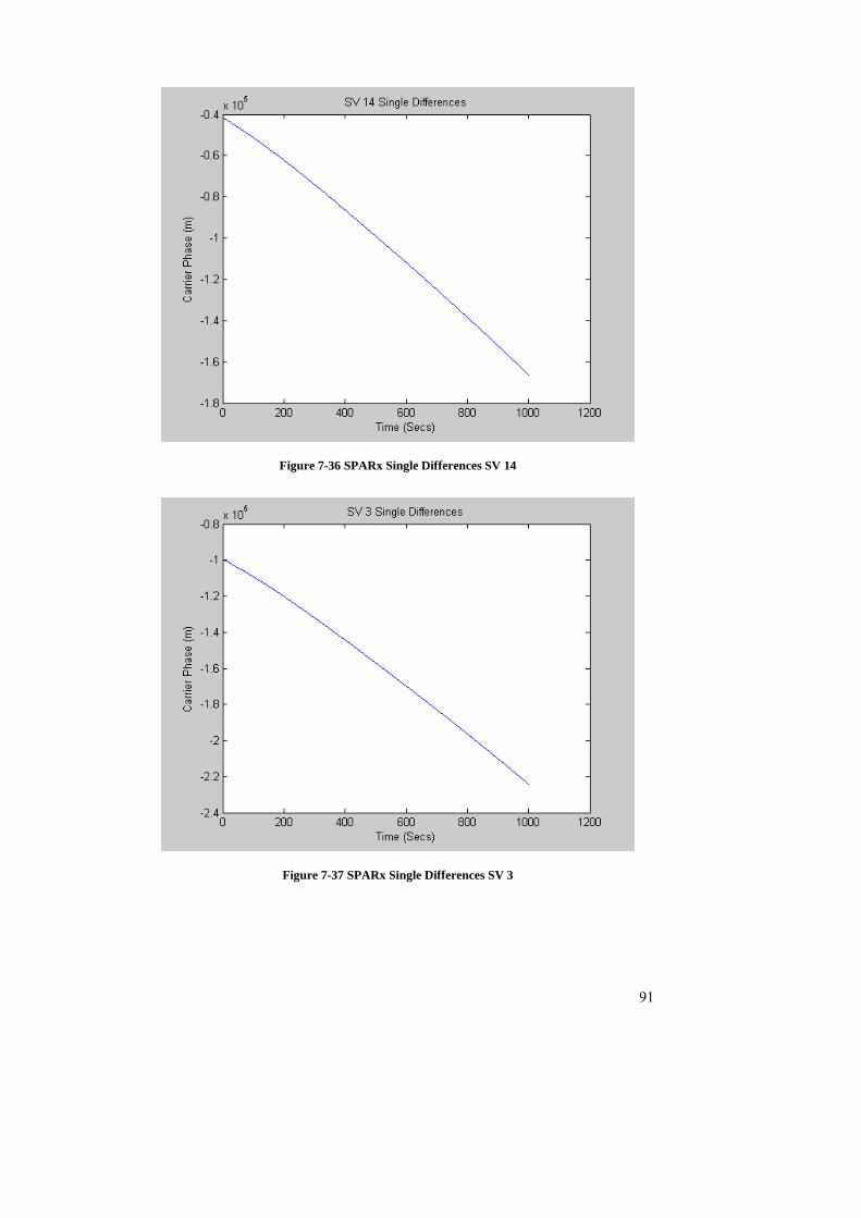
91

Figure 7-36 SPARx Single Differences SV 14

Figure 7-37 SPARx Single Differences SV 3

92

Figure 7-38 shows the double differences for the two SPARx receivers, for satellites

14 and 3.

Figure 7-38 SPARx Double Differences SV 14-3

Figure 7-39 (shown below) is a closer view of a portion of the data shown in Figure 7-38.

Figure 7-39 SPARx Double Differences SV 14-3

93

Figure 7-40 below shows the triple differences for the SPARx receivers which were

formed by differencing the double differenced observable for satellites 14 and 3

between consecutive epochs:

Figure 7-40 SPARx Triple Differences SV 14-3

The statistics for this triple differenced data is given:

Data Statistics

Mean (m) 0.06882

Standard Deviation

(1 sigma) (m) 0.1548

Maximum Deviation

(m) 1.188

Table 7-4 SPARx Triple Differences SV 14-3 Statistics

94

For the Ashtech 3DF data, single differences, double differences and triple

differences were formed as explained in 3.5 using satellites 9 and 7 for over a 4.2

minute period, where satellite 9 had the highest elevation and so was used as the

reference satellite.

Figure 7-41 and Figure 7-42 show the single differences for between antennas 1 and

2 of the 3DF, for satellites 9 and 7.

0 50 100 150 200 250217.5

218

218.5

219

219.5

220

220.5

Time (Secs)

Car

rier P

hase

(m)

SV 9 Single Differences

Figure 7-41 3DF Single Differences SV9

95

0 50 100 150 200 250-513.7

-513.6

-513.5

-513.4

-513.3

-513.2

-513.1

-513

-512.9

-512.8

-512.7

Time (Secs)

Car

rier P

hase

(m)

SV 7 Single Differences

Figure 7-42 3DF Single Differences SV7

Figure 7-43 shows the double differences for between antenna 1 and 2 of the 3DF,

with satellites 9 and 7.

0 50 100 150 200 250-733.5

-733

-732.5

-732

-731.5

-731

Time (Secs)

Car

rier P

hase

(m)

SV 9-7 Double Differences

Figure 7-43 3DF Double Differences SV 9-7

96

Figure 7-44 shows the triple differences for between antennas 1 and 2 of the 3DF.

These were formed by differencing the double differenced observable for satellites 9

and 7 between consecutive epochs:

0 50 100 150 200 250-0.1

-0.08

-0.06

-0.04

-0.02

0

0.02

0.04

0.06

0.08

0.1

Time (Secs)

Car

rier P

hase

(m)

SV 9-7 Triple Differences

Figure 7-44 3DF Triple Differences SV 9-7

The statistics for this triple differenced data is given:

Data Statistics

Mean (m) -0.00751

Standard Deviation

(1 sigma) (m) 0.002208

Maximum Deviation

(m) 0.0118

Table 7-5 3DF Triple Differences SV9-7 Statistics

97

A least squares fit (as done in 7.4.1.1) was made to the double differenced data of the

SPARx and 3DF and residuals plotted for comparison:

Figure 7-45 SPARx Double Difference Residuals SV 14-3

0 50 100 150 200 250-0.5

-0.4

-0.3

-0.2

-0.1

0

0.1

0.2

0.3

0.4

0.5

Time (Secs)

Car

rier P

hase

(m)

residuals

Figure 7-46 3DF Double Differences Residuals SV 9-7

98

7.4.1.4 Conclusions

It can be seen that the SPARx double differences are much noisier by comparing the

double differenced residuals for both the SPARx and 3DF. The comparison for the

triple differences between the SPARx and 3DF also shows this, as given in the table

below.

Triple Difference Data Statistics

SPARx 3DF

Mean (m) 0.06882 -0.00751

Standard Deviation (1 sigma)

(m) 0.1548 0.002208

Maximum Deviation (m) 1.188 0.0118

Table 7-6 SPARx & 3DF Triple Difference Data Statistics

Table 7-6 shows the SPARx performance is poor compared to the 3DF. This large

difference can be explained due to a high multipath environment that the SPARx was

operating under, whereas the 3DF was operating under near perfect conditions. It

must also be noted that these conclusions are based on the double differenced and

triple differenced observables quality without the effect of cycle slips taken into

consideration.

99

Chapter 8 Conclusions and Recommendations

The research presented has covered the specific areas of time synchronization, the

carrier phase implementation and differential GPS using carrier phase as they relate

to SPARx for GPS L1 carrier phase navigation processing. The research has shown

that there is room for improvement with the SPARx to be able to adequately be used

in L1 carrier phase navigation. Access to the source code and hardware designs

makes this a suitable platform for further improvements, new designs and

experimentations of a cost-effective GPS receiver for L1 carrier phase navigation

processing applications.

The research has resulted in the manufacturing of three SPARx as well as the latest

version of SPARx software which includes:

• Time synchronization capability, synchronized to UTC

• Hardware pulse per second output aligned with the integer UTC second

• Integrated L1 carrier phase output in cycles

The use of SPARx in CDGPS was investigated and found that improvements to the

carrier phase are necessary, stated below in 8.2.

A summary of the main individual conclusions and recommendations for the three

areas considered in this research are presented in the following sections.

100

8.1 Time

The tests conducted showed that time synchronization to the receiver’s own

estimation of the integer UTC second was successfully implemented in the receiver

software. After losing synchronization the software successfully realigns the time

and steers the time against the receiver’s own estimation of the integer UTC second.

The timing test results as given in 7.2.1.1 were:

Measurement Time Tag offset from Estimated Integer UTC Second

Value 1 Value 2

Expected

Value

Mean 66.8 ns 2.08 ns -87.5 to 87.5

Standard Deviation

(1 Sigma) 50.6 ns 50.64 ns 50.5 ns

Maximum

Deviation 178 ns 174.6 ns 175 ns

Table 8-1 Time Synchronization Results

This shows that the results are consistent with the expected values as given in 5.2.4.

The spread of the data of approximately 175 nanoseconds is consistent with the TIC

interval resolution limit with the GP2021. The use of the GP2021 for time

synchronization has limitations due to the resolution of 175 nanoseconds which

translates to a clock resolution of 50.5 ns (see 5.2.4.1). The GP4020 is the latest

correlator produced by Zarlink and has the ability for the TIC period to be adjusted in

increments of 25 nanoseconds [20] giving a clock resolution of 7.2 ns RMS. Using

this correlator instead of the GP2021 would result in an improvement.

The comparison between the SPARx and Ashtech μZ-CGRS PPS in 7.2.2 indicated

that on average the SPARx PPS was aligned to UTC within 1.00250 ms, with values

ranging from 1.00198 ms to 1.00400 ms, neglecting any errors in the Ashtech’s PPS.

101

However this is only a rough indication of the absolute accuracy of the SPARx PPS

to the UTC integer second. Ideally, absolute tests need to be carried out such as with

an atomic clock that is synchronized with UTC. The absolute offset between the

SPARx PPS and UTC integer second could then be determined. The software could

be adjusted for accordingly or a time correction factor applied to the measurements

when the absolute offset from the integer UTC second is known. This type of test

could not be made within the time frame given for this research due to the

unavailability of a time laboratory receiver.

8.2 Carrier Phase Processing

Comparisons made with the GPS signal simulator indicated that the carrier phase

was implemented correctly in the SPARx (shown again below in Table 8-2). The

comparison of the carrier phases in 7.4.1.1 indicated that the SPARx carrier phase

variation is slightly worse compared to an Ashtech μZ-CGRS receiver. It was also

observed that the quality of the SPARx carrier phase appears poor when compared

with the Ashtech 3DF receiver in carrier phase differential GPS. These differences

are most likely due to a high multipath environment that the SPARx was operating

under. These conclusions are drawn based on the double differenced and triple

differenced observables quality, without the effect of cycle slips taken into

consideration. The standard deviations of the difference between the range rates

from the carrier phase compared to the simulator’s range rates also indicate poor

quality, of 10 to 18 centimetres variation per second. Values on the order of a few

millimetres are to be expected for a GPS receiver which can be adequately used in

carrier phase navigation processing applications. These tests have shown that there

is room for improving the SPARx carrier phase quality. It is recommended to

improve the current 2nd order FLL carrier phase tracking loop performance by

implementing a 3rd order PLL. This will reduce the noise on the carrier phase

residuals.

102

8.2.1 Carrier Phase in SPARx

Test Results Summary

Simulator Test 1 Mean Range Rate

Offset From

Simulator (m/s)

Standard Deviation Range

Rate Offset From Simulator

(m/s)

Receiver Range Rate 0.1865 m/s NA

Range Rate from

Carrier Phase -0.2221 m/s NA

Simulator Test 2

Range Rate from


Range Rate from


Table 8-2 Simulator Test

The standard deviations of 0.1 and 0.188 m/s (1 sigma ) is equivalent to 10 and 18

cm per second variation on the carrier phase, which indicates the carrier phase

tracking performance is poor.

8.2.2 Carrier Phase Differential GPS

Using the SPARx in carrier phase differential GPS showed that its performance is

poor in comparison with a multi-antenna Ashtech 3DF receiver (for attitude

determination). The comparison for the triple differences between the SPARx and

3DF shows this as given in the table below.

103

Triple Difference Data Statistics

SPARx 3DF

Mean (m) 0.06882 -0.00751

Standard Deviation (1 sigma)

(m) 0.1548 0.002208

Maximum Deviation (m) 1.188 0.0118

Table 8-3 SPARx & 3DF Triple Difference Data Statistics

104

Bibliography

[1] "GPS Orion 12 Channel GPS Reference Design," Mitel Semiconductor AN4808, 2001.

[2] W. Enderle, P. Roberts, T. Bruggemann, and C. Boyd, "GPS Receiver on JaeSat," presented at SatNav 2003 The 6th International Symposium on Satellite Navigation Technology Including Mobile Positioning & Location Services, Melbourne, Australia, 2003.

[3] W. Enderle, C. Boyd, and J. A. King, "Joint Australian Engineering (Micro) Satellite (JAESat) - A GNSS Technology Demonstration Mission," presented at The 2004 International Symposium on GNSS/GPS, Sydney, Australia, 2004.

[4] W. Enderle, Y. Feng, and N. Zhou, "Orbit Determination of FedSat based on GPS Receiver Position Solutions," presented at 14th Australian International Australian Aerospace Congress and 14th National Space Engineering Symposium, Brisbane, Australia, 2003.

[5] O. Montenbruck, M. Markgraf, S. Leung, and E. Gill, "A GPS Receiver for Space Applications," presented at ION GPS 2001, Salt Lake City, Utah, USA, 2001.

[6] D. M. J. Unwin, D. M. K. Oldfield, and S. Purivigraipong, "Orbital Demonstration of a New Space GPS Receiver for Orbit and Attitude Determination," 2000.

[7] O. Montenbruck, E. Gill, M. Markgraf, R. Schulte, and D. Wilde, "GPS Tracking of the IRDT-2 Re-entry Capsule," presented at 16th International Symposium on Spaceflight Dynamics, Pasadena, California, 2001.

[8] "NAVSTAR GPS USER EQUIPMENT INTRODUCTION," September 1996.

[9] B. Hofmann-Wellenhof, H. Lichtenegger, and J. Collins, Global Positioning System: Theory and Practice, 5th ed. New York: Springer-Verlag, 1997.

[10] "Navstar GPS Space Segment/Navigation User Interfaces Rev C," ICD-GPS-200C, 10 Oct 1993.

[11] D. Wells, Guide To GPS Positioning, 1986. [12] P. Misra and P. Enge, Global Positioning System: Signals, Measurements,

and Performance. Lincoln: Ganga-Jumuna Press, 2001. [13] W. Enderle and P. J. Roberts, "GPS Receiver Development for Space

Applications at Queensland University of Technology (QUT)," presented at 10th Australian International Aerospace Congress, Brisbane, Australia, 2003.

[14] "GPS Architect User's Guide," Mitel Semiconductor DM4921, March 1997. [15] "GP2000 GPS Receiver Hardware Design," Mitel Semiconductor AN4855,

1999. [16] "Model TXO200B Product Specification," Rakon Limited, 2000. [17] "TXO200B Test Data Report," Rakon Limited, 2003. [18] "GP2000 GPS Chipset - Designer's Guide," Mitel Semiconductor MS4395,

1998. [19] "GP2021 GPS 12-Channel Correlator," Mitel Semiconductor DS4077, 2001. [20] "GP4020 GPS Baseband Processor Design Manual," Zarlink Semiconductor

DM5280, 2002.

105

[21] W. H. Beyer, "CRC Handbook of Tables for Probability and Statistics," 2nd ed. Cleveland: The Chemical Rubber Co., 1968.

[22] R. Hatch, "Instantaneous Ambiguity Resolution," presented at Kinematic Systems in Geodesy, Surveying, and Remote Sensing, Banff, Alberta, Canada, 1990.

[23] D. Kim and R. B. Langley, "GPS Ambiguity Resolution and Validation: Methodologies, Trends and Issues," presented at International Symposium on GPS/GNSS, Seoul, Korea, 2000.

[24] F. H. Bauer, E. G. Lightsey, J. McCullough, J. O'Donnell, and R. Schnurr, "GADACS: A GPS Attitude Determination and Control Experiment on a Spartan Spacecraft," Control Engineering Practice, vol. 3, pp. 1125-1130, 1995.

[25] Q. P. Chu and P. T. L. M. v. Woerkom, "GPS For Low-cost Attitude Determination," Acta Astronautica, vol. 41, pp. 421-433, 1997.

[26] E. Clarke, E. Cohen, E. G. Lightsey, B. W. Parkinson, and W. Feess, "Space Flight Tests of Attitude Determination Using GPS," International Journal of Satellite Communications, vol. 12, pp. 427-433, 1994.

[27] E. G. Lightsey, C. E. Cohen, and B. W. Parkinson, "Attitude Determination and Control for Spacecraft using Differential GPS," presented at 2nd ESA International Conference on GNC, ESTEC, Noordwijk, 1994.

[28] C. Arbinger, W. Enderle, L. Fraiture, and O. Wagner, "A new algorithm (STAR) for cycle ambiguity resolution within GPS based attitude determination," presented at 4th ESA International Conference on Spacecraft Guidance, Navigation and Control Systems, ESTEC, Noordwijk, The Netherlands, 1999.

[29] S. Yoon and J. B. Lundberg, "An integer ambiguity resolution algorithm for real-time GPS attitude determination," Applied Mathematics and Computation, vol. 129, pp. 21-41, 2002.

[30] J.-C. Juang and G.-S. Huang, "Development of GPS-based attitude determination algorithms," IEEE Transactions on Aerospace and Electronic Systems, vol. 33, pp. 968-976, 1997.

[31] C. R. Cahn, D. K. Leimer, Charles L. Marsh, F. J. Huntowski, and G. D. Larue, "Software Implementation of a PN Spread Spectrum Receiver to Accommodate Dynamics," IEEE Transactions on Communications, vol. 25, 1977.

[32] E. D. Kaplan, Understanding GPS: Principles and Applications. Boston: Artech House, Inc., 1996.

[33] "MicroZ CGRS & iCGRS GPS Receivers Operation & Reference Manual," Thales Navigation, Inc. 2002.

[34] T. Bruggemann and W. Enderle, "Time Synchronization Capability of SPARx - the Queensland University of Technology (QUT) GPS Receivers," presented at GNSS 2004 - The 2004 International Symposium on GNSS/GPS, Sydney, Australia, 2004.

[35] M. Kayton and W. R. Fried, Avionics Navigation Systems, 2nd ed. New York: John Wiley & Sons, Inc., 1997.

gps l1 carrier phase navigation processing · 2010-06-09 · test results conducted in the area of...

Documents