GPS Anti-Jam: A Simple Method of Single AntennaNull-Steering for Aerial Applications

Emily McMilin, David S. De Lorenzo, Thomas Lee, Per Enge: Stanford UniversityDennis Akos: University of Colorado, Boulder

Stefano Caizzone, Andriy Konovaltsev: German Aerospace Center (DLR)

ABSTRACT

In this paper we introduce a backward compatible single an-tenna design for GPS jam mitigation on aircraft. Similar toour prior work in spoof detection [1], this anti-jam antennarequires no additional signal processing at the receiver, and itfits into the form-factor of a standard GPS antenna. There aretwo primary modes of operation. During the default mode,the antenna performs comparable to standard GPS antennas.During the jam mitigation mode, null steering toward the op-timal azimuthal direction will generally provide greater than10 dB of broadband signal suppression from the antenna hori-zon to an elevation angle about 45 below the horizon, alongthat azimuthal 2-D cut.

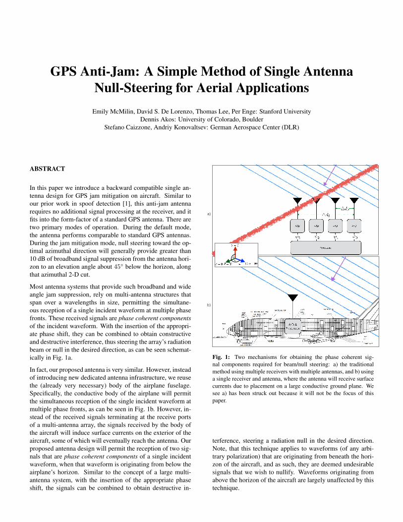
Most antenna systems that provide such broadband and wideangle jam suppression, rely on multi-antenna structures thatspan over a wavelengths in size, permitting the simultane-ous reception of a single incident waveform at multiple phasefronts. These received signals are phase coherent componentsof the incident waveform. With the insertion of the appropri-ate phase shift, they can be combined to obtain constructiveand destructive interference, thus steering the array’s radiationbeam or null in the desired direction, as can be seen schemat-ically in Fig. 1a.

In fact, our proposed antenna is very similar. However, insteadof introducing new dedicated antenna infrastructure, we reusethe (already very necessary) body of the airplane fuselage.Specifically, the conductive body of the airplane will permitthe simultaneous reception of the single incident waveform atmultiple phase fronts, as can be seen in Fig. 1b. However, in-stead of the received signals terminating at the receive portsof a multi-antenna array, the signals received by the body ofthe aircraft will induce surface currents on the exterior of theaircraft, some of which will eventually reach the antenna. Ourproposed antenna design will permit the reception of two sig-nals that are phase coherent components of a single incidentwaveform, when that waveform is originating from below theairplane’s horizon. Similar to the concept of a large multi-antenna system, with the insertion of the appropriate phaseshift, the signals can be combined to obtain destructive in-

2

a)

b)

Fig. 1: Two mechanisms for obtaining the phase coherent sig-nal components required for beam/null steering: a) the traditionalmethod using multiple receivers with multiple antennas, and b) usinga single receiver and antenna, where the antenna will receive surfacecurrents due to placement on a large conductive ground plane. Wesee a) has been struck out because it will not be the focus of thispaper.

terference, steering a radiation null in the desired direction.Note, that this technique applies to waveforms (of any arbi-trary polarization) that are originating from beneath the hori-zon of the aircraft, and as such, they are deemed undesirablesignals that we wish to nullify. Waveforms originating fromabove the horizon of the aircraft are largely unaffected by thistechnique.

SIMULATED PERFORMANCE

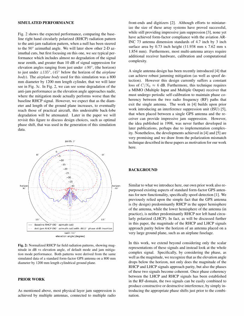
Fig. 2 shows the expected performance, comparing the base-line right hand circularly polarized (RHCP) radiation patternto the anti-jam radiation pattern, when a null has been steeredto the 90 azimuthal angle. We will later show other 2-D az-imuthal cuts, but first focusing on this one, we see typical per-formance which includes almost no degradation of the signalnear zenith, and greater than 10 dB of signal suppression forelevation angles ranging from just under ±90, (the horizon)to just under ±135, (45 below the horizon of the airplanebody). The airplane body used for this simulation was a 800mm diameter by 1200 mm length cylinder, that we will latersee in Fig. 3c. In Fig. 2, we can see some degradation of theanti-jam performance as the elevation angle approaches nadir,where the mitigation mode actually performs worse than thebaseline RHCP signal. However, we expect that as the diam-eter and length of the ground plane increases, to eventuallyreach those of practical aircraft, this undesirable back-lobedegradation will be attenuated. Later in the paper we willrevisit this figure to discuss design choices, such as optimalphase shift, that was used in the generation of this simulationdata.

Fig. 2: Normalized RHCP far field radiation patterns, showing mag-nitude in dB vs elevation angle, of default mode and jam mitiga-tion mode performance. Both patterns were derived from the samesimulated data of a standard form-factor GPS antenna on a 800 mmdiameter by 1200 mm length cylindrical ground plane.

PRIOR WORK

As mentioned above, most physical layer jam suppression isachieved by multiple antennas, connected to multiple radio

front-ends and digitizers [2]. Although efforts to miniatur-ize the size of these array systems have proved successful,while still providing impressive jam suppression [3], none yethave achieved form-factor compliance with the aviation AR-INC 73 antenna dimension standards of 4.7 inch by 3 inchsurface area by 0.73 inch height (11.938 mm x 7.62 mm x1.854 mm). Furthermore, most multi-antenna arrays requireadditional receiver hardware, calibration and computationalcomplexity.

A single antenna design has been recently introduced [4] thatcan achieve robust jamming mitigation (as well as spoof de-tection). However this design currently suffers a constantloss of C/N0 ≈ 6 dB. Furthermore, this technique requiresa MIMO (Multiple Input and Multiple Output) receiver thatmust undergo periodic self-calibration to maintain phase co-herency between the two radio frequency (RF) paths thatexit the single antenna. The work in [4] builds upon priorwork introducing an interference suppression unit (ISU) [5],that when placed between a single GPS antenna and the re-ceiver can provide impressive jam suppression. However,the idea published in 1998, was never further developed inlater publications, perhaps due to implementation complex-ity. Nonetheless, the developments achieved in [4] and [5] arevery promising and we draw from the polarization mismatchtechnique described in these papers as motivation for our workhere.

BACKGROUND

Similar to what we introduce here, our own prior work also re-purposed existing aspects of standard form-factor GPS anten-nas for new functionality, specifically spoof-detection [1]. Wepreviously relied upon the simple fact that the GPS antennais (by design) predominantly RHCP in the upper hemisphereof the antenna, while the lower hemisphere of the antenna (inpractice), is neither predominantly RHCP nor left hand circu-larly polarized (LHCP). In fact, as will be discussed furtherin this paper, the magnitude of the RHCP and LHCP signalsapproach parity below the horizon of an antenna placed on avery large ground plane, such as an airplane fuselage.

In this work, we extend beyond considering only the scalarrepresentations of these signals and instead look at the wholecomplex signal. Specifically, by considering the phase, aswell as the magnitude, we recognize that as the elevation angledrops below the horizon, not only does the magnitude of theRHCP and LHCP signals approach parity, but also the phasesof these two signals become coherent. Once phase coherencybetween the LHCP and RHCP signals has been establishedin the RF-domain, the two signals can be easily combined toproduce constructive or destructive interference, by simply in-troducing the appropriate phase shifts just prior to the combi-nation.

Ground plane effects

To understand the generation of the equal magnitude andphase coherent RHCP and LHCP components, we must con-sider the effect of the ground plane upon waveforms that areoriginating from below the horizon. Fig. 3 shows three differ-ent ground planes, upon which we tested an identical antenna.The antenna is a 30 mm by 30 mm square conductive patch ona 50 mm by 50 mm square substrate with a dielectric constantof 9.8 (modeled after Rogers’ popular TMM 10i ceramic ma-terial). Note that this is the exact same antenna that we willrevisit throughout this paper. The dimensions of the groundplane is all that varied in this experiment: a 73 mm by 73mm square conductive ground plane, a 150 mm by 150 mmsquare conductive ground plane, and a 800 mm by 1200 mmcylindrical ground plane. The latter is our approximate repre-sentation of a airplane fuselage, at the upper size limit that oursimulation system (running ANSYS HFSS [6]) can currentlyhandle. In Fig. 3 we also see the 3-D CAD representations ofthe antenna and its respective ground plane, where the colorson the ground plane model the induced surface currents by anRHCP source.

Fig. 4 shows the magnitude of the RHCP and LHCP farfield patterns associated with each of the three ground planes,along the 90 azimuthal cut (the circumference of the cylin-der), where the RHCP signal is a solid line and the LHCPsignal is a dashed line. In the case of the smallest groundplane data (green trace), we can see from the far field pat-terns that the RHCP and LHCP magnitudes are similar for avery small range of elevation angles around ±130(40) be-low the horizon. For the medium sized ground plane (redtrace), we see approximate parity between the RHCP andLHCP magnitudes at a barely wider range of elevations an-gles around ±120(30) below the horizon. However, for thelargest ground plane (blue trace), we can see that the RHCPand LHCP magnitudes are similar to one another over range ofelevation angles spanning about ±100 to ±140 (10 to 50

below the horizon, respectively), with very good agreementfrom about±115 to±140. We expect this trend to continue,such that as the ground plane size further increases, we expectthe similarities between the RHCP and LHCP magnitudes toalso increase in the lower hemisphere of the antenna.

However as noted above, not only do we require the RHCPand LHCP magnitude to approach parity, we also require theRHCP and LHCP phases to become coherent across a widerange of elevation angles. Fig. 5, shows the phase of theRHCP and LHCP radiation patterns, associated with each ofthe three ground planes in Fig. 3. Again, the RHCP radiationpatterns are a solid line and the LHCP radiation patterns are adashed line, and again the traces representing each of the threeground planes retain the same color as that in Fig. 4. FromFig. 5, we can see that for the entire upper hemisphere of theantenna, the RHCP phase remains relatively flat for all threeground planes sizes. This is to be expected, as a flat phaseresponse across elevation angle in the upper hemisphere is animportant quality for a GPS antenna. Specifically focusing onthe two larger ground planes (red and blue traces), we see that

a)

b)

c)

Ground-plane effect

37

6 cm

10 cm

200 cm

maybe incident waveform does become

vertically polarized (VP), but what about obtaining

phase coherent components of incident waveform?

Fig. 3: Identical GPS antenna (a 30 mm by 30 mm conductive patchon a 50 mm by 50 mm substrate) simulated on three different con-ductive ground planes: a) 73 mm by 73 mm square, b) 150 mm by150 mm square, and c) 800 mm by 1200 mm cylinder. CAD of an-tenna with ground plane showing simulated surface currents rangingfrom strong (red) to weak (blue).

the RHCP phase varies only by less than ±5 throughout theupper hemisphere. Also for these two larger ground planeswe see reasonably good agreement between the RHCP andLHCP phases for elevation angles ranging from about ±90

(the horizon) to about ±135 (45 below the horizon). Fi-nally, note that the wild variation of the LHCP phases nearzenith is of little significance due to the low relatively valueof the LHCP magnitude in this region.

We examine the phase agreement more closely in Fig. 6,which shows the phase difference between the RHCP andLHCP radiation patterns for the three platforms introducedabove. We can see that for the largest ground plane (bluetrace), the phase difference remains relatively flat, hoveringabout −10 ± 5, from an elevation angle of about ±90

(the horizon) to about ±135, (45 below the horizon). Wehave highlighted this region with gray bands. The 150 mmx 150 mm ground plane (red trace) does exhibits a relativelyflat phase difference response over a much more narrow an-gular range. Finally the smallest ground-plane (green trace)shows almost no flat phase difference response over elevation

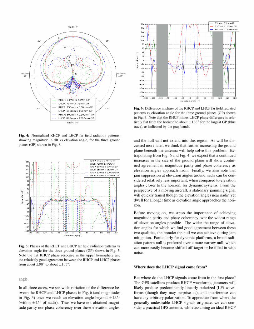
Fig. 4: Normalized RHCP and LHCP far field radiation patterns,showing magnitude in dB vs elevation angle, for the three groundplanes (GP) shown in Fig. 3.

Fig. 5: Phases of the RHCP and LHCP far field radiation patterns vselevation angle for the three ground planes (GP) shown in Fig. 3.Note the flat RHCP phase response in the upper hemisphere andthe relatively good agreement between the RHCP and LHCP phasesfrom about ±90 to about ±135.

angle.

In all three cases, we see wide variation of the difference be-tween the RHCP and LHCP phases in Fig. 6 (and magnitudesin Fig. 3) once we reach an elevation angle beyond ±135

(within ±45 of nadir). Thus we have not obtained magni-tude parity nor phase coherency over these elevation angles,

2

Fig. 6: Difference in phase of the RHCP and LHCP far field radiatedpatterns vs elevation angle for the three ground planes (GP) shownin Fig. 3. Note that the RHCP minus LHCP phase difference is rela-tively flat from the horizon to about ±135 for the largest GP (bluetrace), as indicated by the gray bands.

and the null will not extend into this region. As will be dis-cussed more later, we think that further increasing the groundplane beneath the antenna will help solve this problem. Ex-trapolating from Fig. 6 and Fig. 4, we expect that a continuedincreases in the size of the ground plane will show contin-ued agreement in magnitude parity and phase coherency aselevation angles approach nadir. Finally, we also note thatjam suppression at elevation angles around nadir can be con-sidered relatively less important, when compared to elevationangles closer to the horizon, for dynamic systems. From theperspective of a moving aircraft, a stationary jamming signalwill quickly transit though the elevation angles near nadir, yetdwell for a longer time as elevation angle approaches the hori-zon.

Before moving on, we stress the importance of achievingmagnitude parity and phase coherency over the widest rangeof elevation angles possible. The wider the range of eleva-tion angles for which we find good agreement between thesetwo qualities, the broader the null we can achieve during jammitigation. Particularly for dynamic platforms, a broad radi-ation pattern null is preferred over a more narrow null, whichcan more easily become shifted off-target or be filled in withnoise.

Where does the LHCP signal come from?

But where do the LHCP signals come from in the first place?The GPS satellites produce RHCP waveforms, jammers willlikely produce predominantly linearly polarized (LP) wave-forms (though they may surprise us), and interference canhave any arbitrary polarization. To appreciate from where thegenerally undesirable LHCP signals originate, we can con-sider a practical GPS antenna, while assuming an ideal RHCP

waveform from a satellite overhead (as a reasonable simplifi-cation). When the antenna is illuminated with an ideal RHCPwaveform from directly overhead, it will do a good job of con-verting the waveform into an RHCP signal, with often around80% efficiency. However, in this scenario even very good an-tennas will embody imperfections that convert 1 part per 100(in the case of an axial ratio of 1.6 dB) of the RHCP wave-form into an LHCP signal. As the elevation angle of the satel-lite drops, the antenna’s conversion of RHCP waveforms intoLHCP signals generally increases.

To help understand why this occurs, we can consider the de-composition of the incident RHCP waveform into two orthog-onal electric field components, which are themselves orthog-onal to the direction of the energy propagation. We can callthese two components the x-axis field and y-axis field, distin-guished by color in Fig. 7. Specifically, we see two incidentwaveforms as three distinct moments in time: one waveformapproaching from a high elevation angle with x-axis and y-axis fields indicated in green and blue, respectively, and theother waveform approaching from the horizon with x-axis andy-axis fields indicated in purple and yellow, while the blackarrows indicates the direction of propagation. At the earli-est instance in Fig. 7a, we see that all field components havenear equal magnitudes. However, in the later instances ofFig. 7b and 7c, we can see a large reduction in the magnitudeof the y-axis component in the waveform that is approachingfrom the horizon. This loss in magnitude can be attributed tothe high attenuation experienced by all electromagnetic wavesthat have a component of their electric field that is parallelto a conductive surface. Specifically, from Maxwell’s Equa-tions [8], we know that perfectly conductive surfaces will notsupport the parallel electric field component of an electromag-netic wave, but will propagate the perpendicular electric fieldcomponent. This perpendicular field component presents it-self as a vertically polarized (VP) waveform, to the GPS an-tenna.

The green and light blue sections of the ground planes shownin Fig. 3, provide a qualitative indication of these verticallypolarized fields by highlighting the associated surface currentsthey induce. For signals originating from below the horizon,their journey toward the antenna atop an airplane fuselage re-quires some travel time along the conductive body of the air-plane, thus transforming any arbitrary signal into the only typeof signal that the conductive surface supports: a vertically po-larized one. It is important to emphasize that regardless oforiginal polarization of the incoming waveform, only the ver-tical component will survive propagation along a large con-ductive body. Thus any arbitrary waveform arriving from anelevation angle beneath an antenna placed on a large groundplane, should reach the antenna as a VP waveform.

However, we haven’t fully developed our LHCP origin story.Initially, it may not be obvious at all as to why an incident VPwaveform is synonymous with phase coherent and equal mag-nitude RHCP and LHCP signals. We will use a mathematicalmodel below to show that a VP signal can be decomposed intoa RHCP and a LHCP signal. In fact, any LP signal can be de-

a)

b)

c)

Fig. 7: Two incident waveforms at three distinct moments in time:one waveform approaching from a high elevation angle with x-axisand y-axis field components (green and blue arrows) remaining ofequal magnitude, while the other waveform approaching from thehorizon with x-axis and y-axis fields (purple and yellow arrows)showing a significant magnitude reduction when comparing the y-axis component at a) an earlier time instance, b) a later time instance,c) the last time instance.

composed into a RHCP and a LHCP signal [9]. However fornow, we appeal to the more well known reciprocal argument:any circularly polarized signal can be decomposed into two(spatially and temporally) orthogonal LP signals.

When RHCP energy illuminates a GPS antenna, it often ex-cites two orthogonal linearly polarized modes of the antenna,generating two orthogonal signals. Note that in the case ofcircularly polarized sources, the two resultant linearly polar-ized signals are orthogonal in both space (for example one isparallel to the x-axis and the other is parallel to the y-axis)and orthogonal in time (for example one signal leads the othersignal by 90).

For a standard GPS receiver, these two orthogonal signalsmust be processed in the RF-domain, prior to reaching theradio receiver’s input. This processing transforms the two or-thogonal LP signals (which are separated 90 phase shift in

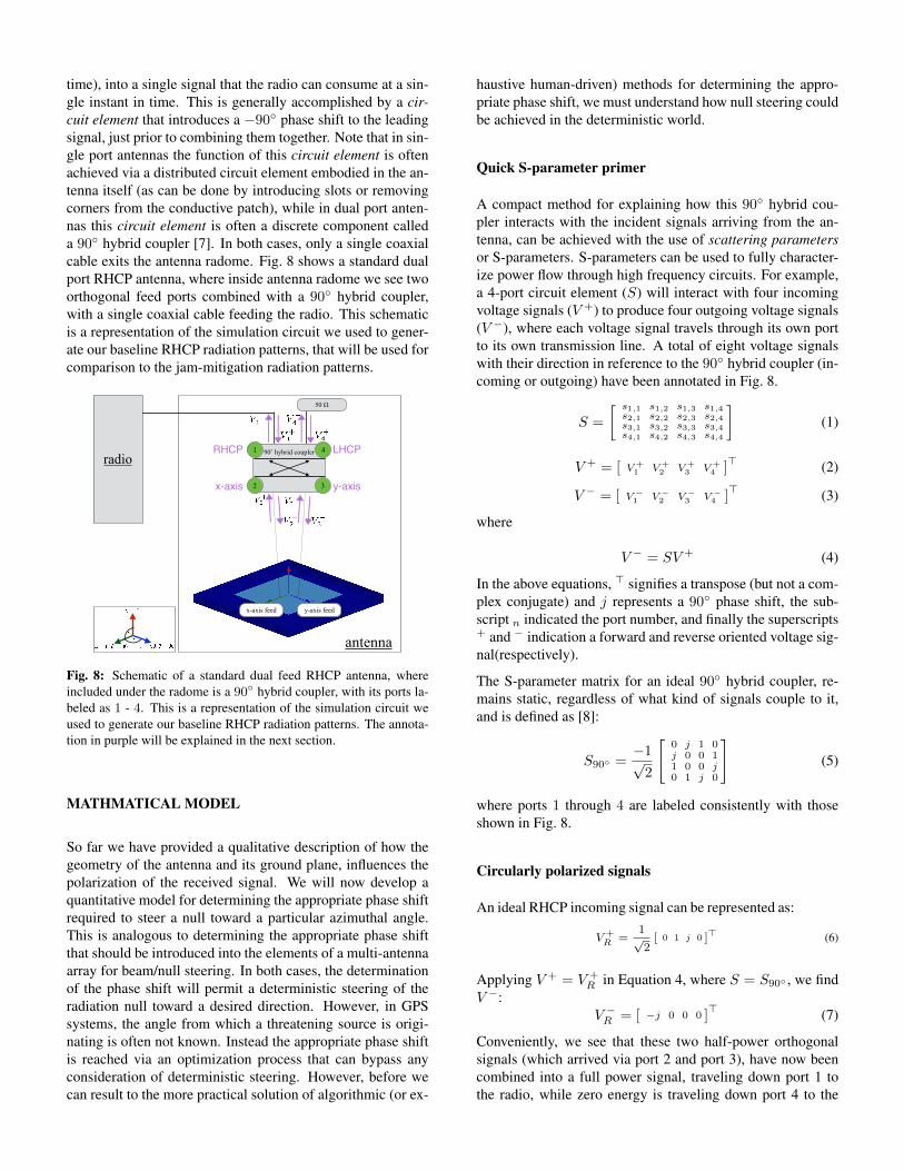
time), into a single signal that the radio can consume at a sin-gle instant in time. This is generally accomplished by a cir-cuit element that introduces a −90 phase shift to the leadingsignal, just prior to combining them together. Note that in sin-gle port antennas the function of this circuit element is oftenachieved via a distributed circuit element embodied in the an-tenna itself (as can be done by introducing slots or removingcorners from the conductive patch), while in dual port anten-nas this circuit element is often a discrete component calleda 90 hybrid coupler [7]. In both cases, only a single coaxialcable exits the antenna radome. Fig. 8 shows a standard dualport RHCP antenna, where inside antenna radome we see twoorthogonal feed ports combined with a 90 hybrid coupler,with a single coaxial cable feeding the radio. This schematicis a representation of the simulation circuit we used to gener-ate our baseline RHCP radiation patterns, that will be used forcomparison to the jam-mitigation radiation patterns.

antenna

radio

50 Ω

90˚ hybrid coupler1

2 3

4

x-axis feed y-axis feed

LHCPRHCP

x-axis y-axis

Fig. 8: Schematic of a standard dual feed RHCP antenna, whereincluded under the radome is a 90 hybrid coupler, with its ports la-beled as 1 - 4. This is a representation of the simulation circuit weused to generate our baseline RHCP radiation patterns. The annota-tion in purple will be explained in the next section.

MATHMATICAL MODEL

So far we have provided a qualitative description of how thegeometry of the antenna and its ground plane, influences thepolarization of the received signal. We will now develop aquantitative model for determining the appropriate phase shiftrequired to steer a null toward a particular azimuthal angle.This is analogous to determining the appropriate phase shiftthat should be introduced into the elements of a multi-antennaarray for beam/null steering. In both cases, the determinationof the phase shift will permit a deterministic steering of theradiation null toward a desired direction. However, in GPSsystems, the angle from which a threatening source is origi-nating is often not known. Instead the appropriate phase shiftis reached via an optimization process that can bypass anyconsideration of deterministic steering. However, before wecan result to the more practical solution of algorithmic (or ex-

haustive human-driven) methods for determining the appro-priate phase shift, we must understand how null steering couldbe achieved in the deterministic world.

Quick S-parameter primer

A compact method for explaining how this 90 hybrid cou-pler interacts with the incident signals arriving from the an-tenna, can be achieved with the use of scattering parametersor S-parameters. S-parameters can be used to fully character-ize power flow through high frequency circuits. For example,a 4-port circuit element (S) will interact with four incomingvoltage signals (V +) to produce four outgoing voltage signals(V −), where each voltage signal travels through its own portto its own transmission line. A total of eight voltage signalswith their direction in reference to the 90 hybrid coupler (in-coming or outgoing) have been annotated in Fig. 8.

S =

[ s1,1 s1,2 s1,3 s1,4s2,1 s2,2 s2,3 s2,4s3,1 s3,2 s3,3 s3,4s4,1 s4,2 s4,3 s4,4

](1)

V + = [ V +1 V +

2 V +3 V +

4 ]> (2)

V − = [ V −1 V −

2 V −3 V −

4 ]> (3)

where

V − = SV + (4)

In the above equations, > signifies a transpose (but not a com-plex conjugate) and j represents a 90 phase shift, the sub-script n indicated the port number, and finally the superscripts+ and − indication a forward and reverse oriented voltage sig-nal(respectively).

The S-parameter matrix for an ideal 90 hybrid coupler, re-mains static, regardless of what kind of signals couple to it,and is defined as [8]:

S90 =−1√

2

[0 j 1 0j 0 0 11 0 0 j0 1 j 0

](5)

where ports 1 through 4 are labeled consistently with thoseshown in Fig. 8.

Circularly polarized signals

An ideal RHCP incoming signal can be represented as:

V +R =

1√2[ 0 1 j 0 ]> (6)

Applying V + = V +R in Equation 4, where S = S90 , we find

V −:V −R = [ −j 0 0 0 ]

> (7)

Conveniently, we see that these two half-power orthogonalsignals (which arrived via port 2 and port 3), have now beencombined into a full power signal, traveling down port 1 tothe radio, while zero energy is traveling down port 4 to the

50 Ω load. Thus it appears an incoming RHCP signal will betransformed into an outgoing signal on port 1, only, and thuswe have labeled port 1 as “RHCP” in Fig. 8. Note the value of−j for the signal at port 1, simply represents a relative phaseshift of −90 for a signal of full magnitude, and doesn’t haveany effect on the absolute value the signal. This is an idealrepresentation of what happens when an RHCP signal arrivesfrom zenith.

To the contrary, we see applying an LHCP signal:

V +L =

1√2[ 0 j 1 0 ]> (8)

to Equation 4, with S = S90 , we get the entire signal travel-ing down port 4 to the 50 Ω load, and nothing heading downport 1 to the receiver:

V −L = [ 0 0 0 −j ]> (9)

Similar to the case above, it can now be seen that an incomingLHCP signal will be transformed into an outgoing signal onport 4, only, and thus we have labeled port 4 as “LHCP” inFig. 8. The attenuation of LHCP signals in the 50 Ω loadis desirable for the suppression of multi-path, during whichRHCP signals will become LHCP after a single bounce off aconductive surface.

A more common scenario, even in the most ideal of circum-stances, will be the inclusion of some LHCP signal in a pre-dominantly RHCP signal. As noted above, this will occur dueto any circularly polarized antenna that doesn’t have a perfectaxial ratio of 1. For example, a slightly more practical pre-dominantly RHCP signal that contains 1% LHCP:

V +

R=

1√2[ 0 0.99+0.01j 0.01+0.99j 0 ]> (10)

will combine with S = S90 , to produce signals where 99%of the signal heading to port 1 and the remaining 1% burningup in the resister at port 4.

V −R

= [ −0.99j 0 0 −0.01j ]> (11)

Vertically polarized signals

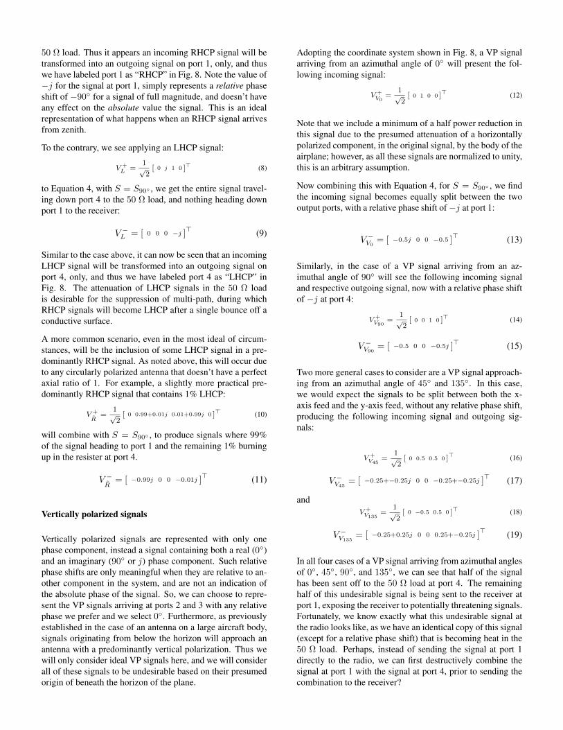
Vertically polarized signals are represented with only onephase component, instead a signal containing both a real (0)and an imaginary (90 or j) phase component. Such relativephase shifts are only meaningful when they are relative to an-other component in the system, and are not an indication ofthe absolute phase of the signal. So, we can choose to repre-sent the VP signals arriving at ports 2 and 3 with any relativephase we prefer and we select 0. Furthermore, as previouslyestablished in the case of an antenna on a large aircraft body,signals originating from below the horizon will approach anantenna with a predominantly vertical polarization. Thus wewill only consider ideal VP signals here, and we will considerall of these signals to be undesirable based on their presumedorigin of beneath the horizon of the plane.

Adopting the coordinate system shown in Fig. 8, a VP signalarriving from an azimuthal angle of 0 will present the fol-lowing incoming signal:

V +V0

=1√2[ 0 1 0 0 ]> (12)

Note that we include a minimum of a half power reduction inthis signal due to the presumed attenuation of a horizontallypolarized component, in the original signal, by the body of theairplane; however, as all these signals are normalized to unity,this is an arbitrary assumption.

Now combining this with Equation 4, for S = S90 , we findthe incoming signal becomes equally split between the twooutput ports, with a relative phase shift of−j at port 1:

V −V0= [ −0.5j 0 0 −0.5 ]

> (13)

Similarly, in the case of a VP signal arriving from an az-imuthal angle of 90 will see the following incoming signaland respective outgoing signal, now with a relative phase shiftof −j at port 4:

V +V90

=1√2[ 0 0 1 0 ]> (14)

V −V90= [ −0.5 0 0 −0.5j ]

> (15)

Two more general cases to consider are a VP signal approach-ing from an azimuthal angle of 45 and 135. In this case,we would expect the signals to be split between both the x-axis feed and the y-axis feed, without any relative phase shift,producing the following incoming signal and outgoing sig-nals:

V +V45

=1√2[ 0 0.5 0.5 0 ]> (16)

V −V45= [ −0.25+−0.25j 0 0 −0.25+−0.25j ]

> (17)

andV +V135

=1√2[ 0 −0.5 0.5 0 ]> (18)

V −V135= [ −0.25+0.25j 0 0 0.25+−0.25j ]

> (19)

In all four cases of a VP signal arriving from azimuthal anglesof 0, 45, 90, and 135, we can see that half of the signalhas been sent off to the 50 Ω load at port 4. The remaininghalf of this undesirable signal is being sent to the receiver atport 1, exposing the receiver to potentially threatening signals.Fortunately, we know exactly what this undesirable signal atthe radio looks like, as we have an identical copy of this signal(except for a relative phase shift) that is becoming heat in the50 Ω load. Perhaps, instead of sending the signal at port 1directly to the radio, we can first destructively combine thesignal at port 1 with the signal at port 4, prior to sending thecombination to the receiver?

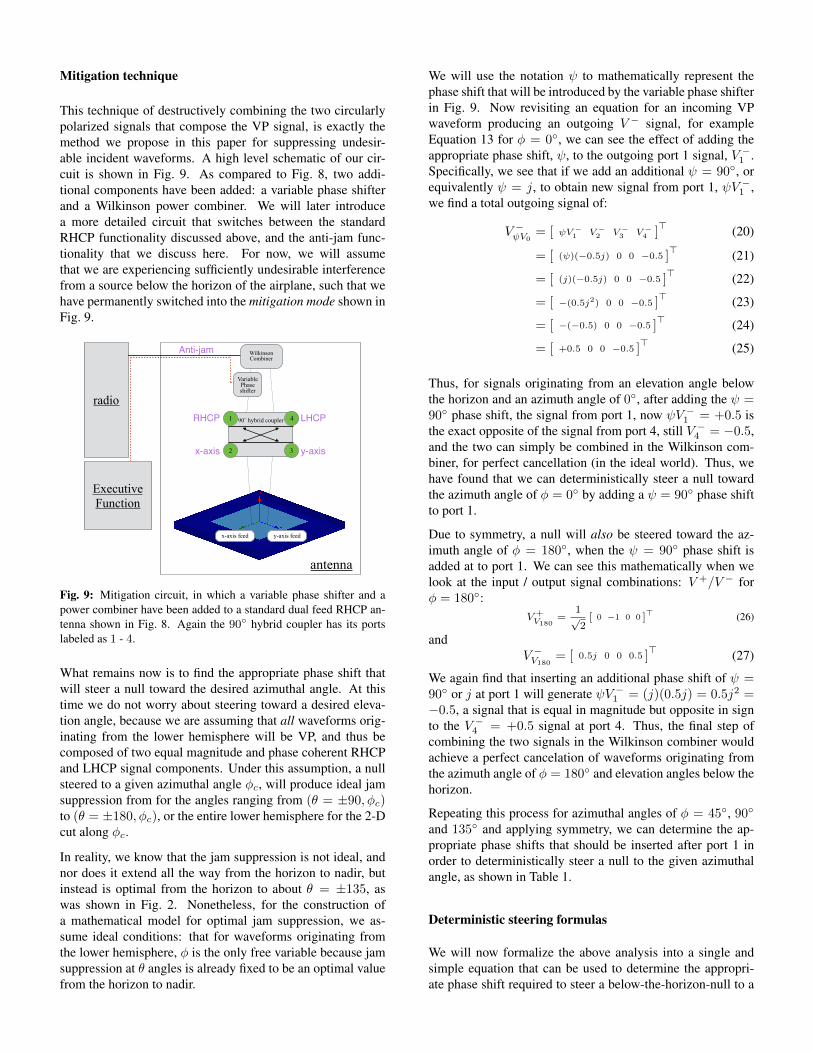
Mitigation technique

This technique of destructively combining the two circularlypolarized signals that compose the VP signal, is exactly themethod we propose in this paper for suppressing undesir-able incident waveforms. A high level schematic of our cir-cuit is shown in Fig. 9. As compared to Fig. 8, two addi-tional components have been added: a variable phase shifterand a Wilkinson power combiner. We will later introducea more detailed circuit that switches between the standardRHCP functionality discussed above, and the anti-jam func-tionality that we discuss here. For now, we will assumethat we are experiencing sufficiently undesirable interferencefrom a source below the horizon of the airplane, such that wehave permanently switched into the mitigation mode shown inFig. 9.

radio

Executive Function

antenna

x-axis feed y-axis feed

90˚ hybrid coupler

Wilkinson Combiner

Variable Phase shifter

3

1

2 3

4 LHCPRHCP

x-axis y-axis

Anti-jam

Fig. 9: Mitigation circuit, in which a variable phase shifter and apower combiner have been added to a standard dual feed RHCP an-tenna shown in Fig. 8. Again the 90 hybrid coupler has its portslabeled as 1 - 4.

What remains now is to find the appropriate phase shift thatwill steer a null toward the desired azimuthal angle. At thistime we do not worry about steering toward a desired eleva-tion angle, because we are assuming that all waveforms orig-inating from the lower hemisphere will be VP, and thus becomposed of two equal magnitude and phase coherent RHCPand LHCP signal components. Under this assumption, a nullsteered to a given azimuthal angle φc, will produce ideal jamsuppression from for the angles ranging from (θ = ±90, φc)to (θ = ±180, φc), or the entire lower hemisphere for the 2-Dcut along φc.

In reality, we know that the jam suppression is not ideal, andnor does it extend all the way from the horizon to nadir, butinstead is optimal from the horizon to about θ = ±135, aswas shown in Fig. 2. Nonetheless, for the construction ofa mathematical model for optimal jam suppression, we as-sume ideal conditions: that for waveforms originating fromthe lower hemisphere, φ is the only free variable because jamsuppression at θ angles is already fixed to be an optimal valuefrom the horizon to nadir.

We will use the notation ψ to mathematically represent thephase shift that will be introduced by the variable phase shifterin Fig. 9. Now revisiting an equation for an incoming VPwaveform producing an outgoing V − signal, for exampleEquation 13 for φ = 0, we can see the effect of adding theappropriate phase shift, ψ, to the outgoing port 1 signal, V −1 .Specifically, we see that if we add an additional ψ = 90, orequivalently ψ = j, to obtain new signal from port 1, ψV −1 ,we find a total outgoing signal of:

V −ψV0= [ ψV −

1 V −2 V −

3 V −4 ]> (20)

= [ (ψ)(−0.5j) 0 0 −0.5 ]> (21)

= [ (j)(−0.5j) 0 0 −0.5 ]> (22)

= [ −(0.5j2) 0 0 −0.5 ]> (23)

= [ −(−0.5) 0 0 −0.5 ]> (24)

= [ +0.5 0 0 −0.5 ]> (25)

Thus, for signals originating from an elevation angle belowthe horizon and an azimuth angle of 0, after adding the ψ =90 phase shift, the signal from port 1, now ψV −1 = +0.5 isthe exact opposite of the signal from port 4, still V −4 = −0.5,and the two can simply be combined in the Wilkinson com-biner, for perfect cancellation (in the ideal world). Thus, wehave found that we can deterministically steer a null towardthe azimuth angle of φ = 0 by adding a ψ = 90 phase shiftto port 1.

Due to symmetry, a null will also be steered toward the az-imuth angle of φ = 180, when the ψ = 90 phase shift isadded at to port 1. We can see this mathematically when welook at the input / output signal combinations: V +/V − forφ = 180:

V +V180

=1√2[ 0 −1 0 0 ]> (26)

andV −V180

= [ 0.5j 0 0 0.5 ]> (27)

We again find that inserting an additional phase shift of ψ =90 or j at port 1 will generate ψV −1 = (j)(0.5j) = 0.5j2 =−0.5, a signal that is equal in magnitude but opposite in signto the V −4 = +0.5 signal at port 4. Thus, the final step ofcombining the two signals in the Wilkinson combiner wouldachieve a perfect cancelation of waveforms originating fromthe azimuth angle of φ = 180 and elevation angles below thehorizon.

Repeating this process for azimuthal angles of φ = 45, 90

and 135 and applying symmetry, we can determine the ap-propriate phase shifts that should be inserted after port 1 inorder to deterministically steer a null to the given azimuthalangle, as shown in Table 1.

Deterministic steering formulas

We will now formalize the above analysis into a single andsimple equation that can be used to determine the appropri-ate phase shift required to steer a below-the-horizon-null to a

azimuthal angles (φ) inserted phase shift (ψ)0 & 180 −270

45 & 225 −180

90 & 270 −90

135 & 315 0

Table 1: Phase shift (ψ) that must be inserted to achieve determin-istic steering of a null to azimuthal angle, φ, and to elevations anglesbeneath the horizon. Note that due to symmetry, a ψ has double theperiodicity of φ.

given azimuthal angle. However, we will first revisit the morefamiliar scenario of the multi-antenna array shown in Fig. 1a.In this multi-antenna array, to deterministically steer a beam toan elevation angle θ, we would introduce the following phaseshift, ψi, to the ith element of the array [9]:

ψi = 2π4diλ

sin θ + ψ0 (28)

where

d0 = location of reference antennaψ0 = initial phase offset of antenna at d04di = di − d0θ = desired elevation angle for beam

(29)

Similarly, we can extrapolate from the work done in the priorsection to develop a closed form expression for deterministicnull steering in our anti-jam antenna. We precede this equa-tion with that for multi-antenna steering, in order to highlightthe similarities between these two methods. Specifically, inour anti-jam antenna, to deterministically steer a null to an az-imuthal angle φ, we would introduce the following phase shiftψ, to port 1 of the 90 hybrid coupler:

ψ = 24φ+ ψ0 (30)

where

φ0 = orientation of antennaψ0 = initial phase offset of antenna at φ04φ = φ− φ0φ = desired azimuthal angle for null

(31)

For the case of the coordinate system and orientation we usedabove: setting φ0 = 0 and ψ0 = −270, we can see thereis agreement between the outcomes of this formula and thevalues in Table 1.

SYSTEM DESIGN

In practice, our simulation performance rarely conformed tothe ideal behavior of Equation 30. Revisiting Fig. 6, recallthat the 800 mm x 1200 mm cylindrical ground plane showed

a phase difference between the RHCP and LHCP signals thatwas relatively flat over a good portion of the elevation anglesbelow the horizon. However, instead of the phase differencehovering about 0 ± 5, as expected for a VP signal, we seea phase difference hovering about 10 ± 5. Hence we seean additional, thus far unaccounted for, 10 geometry-basedphase offset. At this time, it is unclear how the geometry ofthe ground-plane and the antenna affect this deviation fromexpectation. However we do see that it is based on geome-try of the ground-plane and that is a function of φ. To ac-count for this geometry-based phase offset, we must modifyEquation 30 to introduce an additional ψ component that is afunction of φ:

ψ = 24φ+ ψ0 + ψφ (32)

where, in addition to Equations 31, we must add:

ψφ = geometry-based phase offset as a function of φ(33)

For this paper, we determine a reasonable ψφ by using thetechnique discussed in the beginning of this section. Specif-ically, we plot the phase difference between the RHCP andLHCP signals for each azimuthal angle of interest, and thenlook for the deviation from the expected phase difference ofabout 0±5. Returning to the example we began in this sec-tion, for an azimuthal angle of 90, Equation 30 predicts anoptimal phase shift insertion value of −90. However for thecase of the 800 mm x 1200 mm cylindrical ground plane, wemust include the ψφ = 10 phase difference offset shown inFig. 6, to reach a final optimal phase shift insertion value of−80 (as was used in Fig. 2).

We now will look qualitatively at the expected radiation pat-terns for both the default RHCP radiation pattern and ouranti-jam pattern for the first quadrant of the sphere. Due totwo bilateral symmetries, we expect the remaining 3 quad-rants to resemble the one shown here. Specifically, we lookat 2-D elevation cuts along constant azimuth angles of φ =0, 30, 60 in Fig. 10 (and φ = 90 was already seenin Fig. 2), where we have steering a null to each given az-imuth angle. We see anti-jam performance generally meet-ing our expectations stated earlier: greater than about 10 dBof jam suppression from the horizon to about 45 below thehorizon, and generally an un-modified upper hemisphere re-sponse. As we have noted before, jam suppression for the re-maining lower hemisphere elevation angles (from about 45

below the horizon to nadir) is more dependent on the form-factor of the aircraft, and we expect improved performancein this region when the proposed antenna design is tested onlarger aircrafts. We also claim that the relative importance ofjam suppression is reduced as elevation angles approach nadir,due to the limited dwell time that a static spoofer will remainin at this elevation angle relative to an antenna on a movingplatform, when compared to elevation angles that approachthe horizon.

The results seen in Fig. 10 and 2, were achieved by taking theraw data (of the x-axis and y-axis electric field components of

2

a)

b)

c)

Fig. 10: Normalized RHCP far field radiation patterns, showingmagnitude in dB vs elevation angle, of default mode and jam mitiga-tion mode for the first quadrant of the simulated data, derived fromthe same dataset that was a first introduced in Fig. 2

the far field plot) from HFSS and post-processing in Python tosimulate the 90 hybrid coupler, phase shifter and Wilkinsonpower combiner. Python scripts permitted systematic batchprocessing of large simulation files. However manual checkswere performed in ANSYS Designer [6] circuit simulator tospot check the validity of the Python results.

Practical phase shifting

So far we have discussed a deterministic mapping between anazimuthal angle of interest and the proper phase shift selec-tion. The main purpose of explaining the math behind thismapping is to motivate the relationship between the variablephase shifter and the azimuthal angle of the null steering. Inthis section we discuss a more practical mapping between thephase insertion applied at the variable phase shifter and ourdesired goal of jam suppression.

Adjustment of the phase shifter up in the antenna from a loca-tion down at the receiver, could be implemented with a sim-ple circuit that is essentially the size of an RF barrel connec-tor. This added circuit places the control voltage onto the in-ner conductor of the RF coaxial cable and could consist of asmall battery, an exposed switch or dial, an RF choke, a DCblocking capacitor and a couple resisters. Note that here wehave assumed that an analog phase shifter (such as the HittiteHMC934LP5E) is used at the antenna, thus requiring only asimple change in DC control voltage level for the adjustmentof the variable phase shift. Note that there will be severalcomponents requiring control and supply voltages in the an-tenna, and thus a more sophisticated system of coupling lowfrequency AC voltage control signals may be required.

The exposed dial could be controlled by a human operator,effectively tuning the antenna for an optimal response. How-ever, a more desirable implementation could involve integra-tion with a standard GPS receiver to include a power mini-mization algorithm running on the receiver in the digital do-main. This algorithm can adapt a DC (or low frequency mod-ulated AC) voltage control signal, that is coupled onto the in-ner (or outer) conductor of the RF coaxial cable, in order toestablish an optimal phase shift. We will briefly introduce onepossible mechanism for this algorithm.

All receivers have an analog to digital converter (ADC) thatfollows the analog radio front-end, and proceeds the digitalacquisition and tracking algorithms. After the ADC, the ana-log signal captured by the receiver is now a digital sequencen bits long, where n is the fixed number of bits used by theADC during the conversion. For reasons soon addressed, anyreceiver with an ADC where n < 1, will also contain an au-tomatic gain control (AGC) component [10]. ADCs have alimited dynamic range of power levels under which they canoptimally convert the incoming analog signals into their dig-ital counterparts. Thus in order to capture the largest rangeof incoming signals, it is desirable to place the average signalpower in the middle of the ADC’s dynamic range, and this isthe job of the AGC.

For a quick example, we use a two bit ADC where < 00 >represents the weakest signal and < 11 > represents thestrongest. If the AGC fails to center the average signal powerin middle of this range, and instead lets it drift upward, wemay find our measured samples all appear to be < 11 >without variation, and thus important information has been”clipped” away and forever lost. It should also be noted thatalthough the GPS signal power is below the thermal noisefloor, the power level of the noise signal can undergo fluc-tuations and slow drifts that require an AGC to maintain op-timal dynamic range at the receiver [10]. A final point worthmentioning, is that most AGCs can operate on time constantsof microseconds [12], thus several orders of magnitude fasterthan the integration dump period of a standard GPS receiver.We therefore do not experience loss of carrier lock or otherill-effects, one might expect from a sluggish AGC.

So, we propose, as has been proposed before [11], that theAGC could be one optimal, low complexity and backwardcompatible mechanism for implementing the PM algorithm.Full receiver integration would only require a firmware up-grade that links the output of the AGC to the voltage signalthat controls the phase shifter in the antenna, within feedbackloop that will settle at the AGC’s default (interference-free)baseline level.

Circuit implementation

As we mentioned previously, the results in Fig. 10 and 2,were achieved post-processing raw simulation antenna radi-ation pattern data with Python scripts to simulate the 90 hy-brid coupler, phase shifter and Wilkinson power combiner.Despite the good agreement we see between the circuit sim-ulation and the Python implementation, some non-idealitiescan get more easily brushed away when relying on Pythonscripts alone. For example it may not be obvious that theWilkinson power combiner will sometimes (but not always)incur an insertion loss of greater than 3 dB. This is not in-tuitive because when the Wilkinson component is used in areciprocal manner as a power splitter, the insertion loss isusually closer to 0.5 dB. If composed of ideal materials, andperfectly impedance matched, the insertion loss of the powersplitter would be 0 dB, or perfectly loss-less. This apparentinconsistency is because even ideal 3 port network devicessuch as the idealized representation of a Wilkinson powercombiner/splitters is loss-less when acting as a power split-ter and only in certain scenarios when acting as a power com-biner. These losses are incurred in the power combiner ar-rangement, despite our assumption of ideal materials and per-fect impedance matching [8].

A quick example can serve to illustrate: a 3 dBm signal powerat the combined output port of such a combiner can be derivedin one of many ways, including the two following scenarios:a) phase coherent 0 dBm signals at both input ports, or b)a non-phase coherent combo of −∞ dBm at one input portand 6 dBm at the other input port. In scenario (a) we have aloss-less combination of the two signals, but in scenario (b)

we have lost half our signal power. Where does this signalpower go? The answer to this question is that there is in fact aresister that is hidden inside the Wilkinson power divider (be-tween the two input ports). When the signals presented at thetwo input are identical (as is the case in scenario (a)), thereis no current flowing across this internal resister because thevoltage levels on either side of the resister are identical [13].However, in scenario (b) when one input signal is approaching−∞ dBm, we will find that half the power of the other signalwill be dropped across the internal resister. For the predomi-nantly VP signals originating from the lower hemisphere, wehave scenario (a) in which the two input signals (namely theRHCP and the LCHP signals) will be combined in an almostloss-less fashion, whereas for signals originating at zenith wehave scenario (b), in which we lose about 3 dB from this pre-dominately RHCP signal that is arriving at one input (whilethe 2nd input port is around -20 dBm. Thus we have the sce-nario where 3 dB of loss could be incurred at zenith, but notalong the horizon.

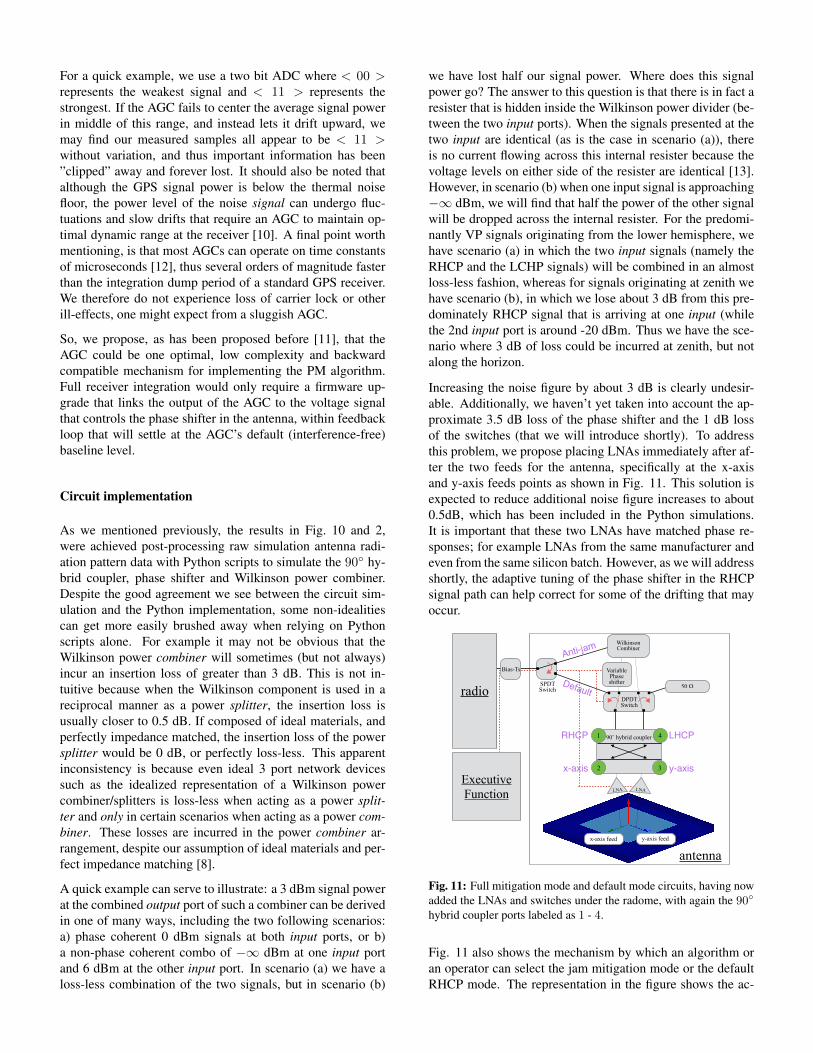
Increasing the noise figure by about 3 dB is clearly undesir-able. Additionally, we haven’t yet taken into account the ap-proximate 3.5 dB loss of the phase shifter and the 1 dB lossof the switches (that we will introduce shortly). To addressthis problem, we propose placing LNAs immediately after af-ter the two feeds for the antenna, specifically at the x-axisand y-axis feeds points as shown in Fig. 11. This solution isexpected to reduce additional noise figure increases to about0.5dB, which has been included in the Python simulations.It is important that these two LNAs have matched phase re-sponses; for example LNAs from the same manufacturer andeven from the same silicon batch. However, as we will addressshortly, the adaptive tuning of the phase shifter in the RHCPsignal path can help correct for some of the drifting that mayoccur.

antennax-axis feed y-axis feed

90˚ hybrid coupler

Wilkinson Combiner

DPDT Switch

SPDT Switchradio 50 Ω

LNA LNA

Variable Phase shifter

4

Anti-jam

Default

Executive Function

Bias-Ts

1

2 3

4 LHCPRHCP

x-axis y-axis

Fig. 11: Full mitigation mode and default mode circuits, having nowadded the LNAs and switches under the radome, with again the 90

hybrid coupler ports labeled as 1 - 4.

Fig. 11 also shows the mechanism by which an algorithm oran operator can select the jam mitigation mode or the defaultRHCP mode. The representation in the figure shows the ac-

tive mode as the jam mitigation mode the switches. We willcomplete final component selection for prototyping in futurework. However at the present time, we have identified likelycandidates for these components as shown in Table 2.

component manufacturer part numberDPDT switch Skyworks SKY13381-374LFSPDT switch Skyworks SKY13370-374LF

90 hybrid coupler Anaren C1517J5003AHFPhase shifter Hittite HMC934LP5E

Wilkinson combiner Anaren PD0922J5050S2HFLNA Avago MGA-634P8

Table 2: Components that are good candidates for implementation.

Summation mode

A question remains in regard to what happens at all the otherazimuthal angles when a null is being steered toward one par-ticular azimuth angle? We know that the phase shift insertionvalue of ψ has twice the periodicity of the azimuthal angle φ,so, we would expect that steering a null toward an azimuthangle φc will also produce a null at azimuth angle φc + 180.Thus, appealing to symmetry, we can expect optimal jam sup-pression responses at azimuth angles separated by 180. Alsoappealing to symmetry, we can expect worst case jam sup-pression responses at azimuth angles separated by φc ± 90,when a null has been steered to φc.

To first get a quantitive sense of this worst case jam suppres-sion, we consider mathematically what would happen whenwe apply the deterministic phase shift required to steer a nullto an azimuth angle of φc = 90, while examining the sig-nal response for a waveform arriving from an azimuth angleof φc − 90 = 0. To deterministically steer a null towardφ = 90, we would use a phase shift of ψ = −90, so weapply this ψ = −90 to the equation for a lower hemisphereVP waveform arriving from azimuth angle of φ = 0 (Equa-tion 13):

V −ψV0= [ (ψ)(0.5j) 0 0 0.5 ]

> (34)

= [ (−j)(0.5j) 0 0 0.5 ]> (35)

= [ −(0.5j2) 0 0 0.5 ]> (36)

= [ −(−0.5) 0 0 0.5 ]> (37)

= [ 0.5 0 0 0.5 ]> (38)

We again find that inserting an additional phase shift of ψ =90 or j at port 1 will generate ψV −1 = (j)(0.5j) = 0.5j2 =−0.5, a signal that is equal in magnitude but opposite in signto the V −4 = +0.5 signal at port 4. Thus, the final step ofcombining the two signals in the Wilkinson combiner wouldachieve a perfect cancelation of waveforms originating fromthe azimuth angle of φ = 180 and elevation angles below thehorizon.

Rather than producing signals at port 1 and 4 that are op-posite of one another, we have produced identical signals:ψV −1 = 0.5 and V −4 = 0.5. Thus, the combined signal willdouble in magnitude at the Wilkinson combiner. So, we seethat at azimuthal angles orthogonal to the direction of nullsteering, we will get summation of the RHCP and LHCP com-ponent signals, rather than cancellation. At azimuthal anglesin between the two theoretical extremes of perfect cancella-tion and perfect summation, we expect to see a smooth transi-tion.

The summation signal is particularly concerning, because aswas the case for the cancellation occurring primarily in thelower hemisphere of the antenna, so will this summation oc-cur primarily in the lower hemisphere of the antenna. Thus wecould be exposing the antenna to even more threatening sig-nals from below. This can be seen in qualitatively in Fig. 12,where in simulation we looked at the radiation pattern for the0 azimuthal cut, after steering a null toward a 90 azimuthalangle.

Fig. 12: Normalized RHCP far field radiation patterns, showingmagnitude in dB vs elevation angle, of default mode and jam mit-igation mode for the 0 azimuthal cut, when a null has been steeredto an orthogonal 90 azimuthal angle.

Larger ground planes

Examination of Fig. 12, and further consideration of our ex-pectations as the ground plane size scales up, present a lessdire outlook than that of the prior paragraph. We are moreaccustomed to seeing the typical GPS antenna patterns withrelatively small ground planes, and in free-space simulationsor measurement (for example those shown in Fig. 3a and 3b)

where the back lobe is dominated by the LHCP radiation pat-tern. However, for larger ground planes, we no longer see aback lobe domination of LHCP, and we instead see are morelikely to see the LHCP radiation pattern creeping up into thelower elevations of the upper hemisphere of the antenna. Inaddition to our simulated data in Fig. 3c, we see both mea-sured and simulated data from relatively larger aircraft groundplanes in Figs. 13 [15] and 14 [14], respectively. All three ofthese figures show that in the lower hemisphere, the magni-tude of RHCP and LHCP signals approach parity, and thatthe LHCP signal has a more significant presence in the up-per hemisphere, particularly at the lower elevation angles. Allthis helps us conclude that although the summation behaviorwill undesirably increase sensitivity in the lower hemisphere,it may also have a desired effect of increasing the sensitivity ofthe antenna in the upper hemisphere, particularly at low anglesof elevation. This presents another potential feature of this an-tenna: when jamming is not present and increased sensitivityis desired at low angles of elevation near the horizon, for ex-ample during landing, take-off or sharp banked curves, theantenna can be switched to this summation mode. Howeverwe also face the presently unresolvable problem that whenjamming sources are located at widely separated angles alongthe horizon of the plane (particularly when two jammers areat right angles to one another), the mitigation mode of the an-tenna may cause more harm than good.

3

Fig. 13: Measured RHCP and LHCP patterns on the fuselage of ascaled-down F-16 jet [14].

We also use Fig. 13 and 14 to help justify our claims thatjam suppression in the back lobe will improve as the groundplane increases in size. Both of these results show very goodagreement between the magnitudes of the RHCP and LHCPsignals at elevation angles within 45 of nadir, which is wherewe saw divergence of the RHCP and LHCP signals from oursimulated data. Unfortunately, we have only magnitude infor-mation and not phase information for the two plots shown inFig. 13 and 14. But based on our evaluation in this paper, we

2

Fig. 14: Simulated RHCP and LHCP patterns on the fuselage of aairplane-like object [15].

expect phase coherency between the RHCP and LHCP signalsas well.

CONCLUSIONS AND FUTURE WORK

In this paper we have introduced a single antenna design forGPS jam mitigation in aircraft applications. We have de-scribed a deterministic method of null-steering the antennaand discussed more practical methods for nulling interference.We have shown simulation results that achieve greater than10 dB of broadband signal suppression from near the antennahorizon to about 45 below the horizon, when the antenna hasbeen null steered toward a given azimuthal angle. The dataprovided was simulated on a 800 mm diameter by 1200 mmlength cylindrical ground plane, and we have provided evi-dence for our expectation of superior performance on larger,aircraft-sized ground plane structures.

Similar to our prior work, we have exploited aspects of ex-isting antennas and associated infrastructure to introduce newfunctionality. In this case we introduced jam mitigation andour prior work developed spoof-detection. Future work willbe directed toward the integration of these two features into astandard form-factor GPS antenna that has been designed foraviation applications. We also intend to prototype and providereal measurement data in future work.

ACKNOWLEDGMENTS

The research conducted for this paper took place at the Stan-ford University Global Positioning System Research Labora-tory with funding from the WAAS program office under FAACooperative Agreement 12-G-003.

REFERENCES

[1] E. McMilin, D. S. De Lorenzo, T. Walter, T. H. Lee,P. Enge, “Single Antenna GPS Spoof Detection that isSimple, Static, Instantaneous and Backward Compatible

for Aerial Applications,” Proceedings of the 27th Inter-national Technical Meeting of The Satellite Division ofthe Institute of Navigation (ION GNSS+ 2014), Tampa,FL, September 2014, pp. 2233-2242.

[2] Y.-H. Chen, S. Lo, D. Akos, D. S. De Lorenzo,P. Enge, “Validation of a Controlled Reception Pat-tern Antenna (CRPA) Receiver Built From Inexpen-sive General-purpose Elements During Several Live-jamming Test Campaigns,” Proceedings of the 2013 In-ternational Technical Meeting of The Institute of Navi-gation, San Diego, California, January 2013, pp. 154-163.

[3] A. Konovaltsev, S. Caizzone, M. Cuntz, M. Meurer,“Autonomous Spoofing Detection and Mitigation with aMiniaturized Adaptive Antenna Array,” Proceedings ofthe 27th International Technical Meeting of The Satel-lite Division of the Institute of Navigation, Tampa, FL,September 2014, pp. 2853-2861

[4] T. Kraus, F. Ribbehege and B. Eissfeller, “Use of theSignal Polarization for Anti-jamming and Anti-spoofingwith a Single Antenna,” Proceedings of the 27th Inter-national Technical Meeting of The Satellite Division ofthe Institute of Navigation, Tampa, FL, September 2014,pp. 3495-3501.

[5] M. W. Rosen, M. S. Braasch, “Low-Cost GPS Inter-ference Mitigation Using Single Aperture CancellationTechniques,” Proceedings of the 1998 National Techni-cal Meeting of The Institute of Navigation, Long Beach,CA, January 1998, pp. 47-58.

[6] ANSYS, “HFSS”, http://www.ansys.com/Products/Simulation+Technology/Electronics/Signal+Integrity/ANSYS+HFSS

[7] B. Rama Rao, W. Kunysz, R. L. Fante and K. F. McDon-ald, GPS/GNSS Antennas, Artech House, 2013

[8] D. M. Pozar, Microwave Engineering, 4th Ed., John Wi-ley & Sons, 2012, pp. 343.

[9] W. L. Stutzman, Polarization in Electromagnetic Sys-tems, Artech House, 1993, pp. 24.

[10] D. Akos, “Who’s Afraid of the Spoofer? GPS/GNSSSpoofing Detection via Automatic Gain Con-trol (AGC)”, Navigation, 59: 281-290. doi:10.1002/navi.19.

[11] F. Bastide, D. Akos, C. Macabiau, B. Roturier “Auto-matic Gain Control (AGC) as an Interference Assess-ment Tool”, Proceedings of the 16th International Tech-nical Meeting of the Satellite Division of The Instituteof Navigation (ION GPS/GNSS 2003), Portland, OR,September 2003, pp. 2042-2053.

[12] Maxim Integrated, MAX2769, “UniversalGPS Receiver”, http://datasheets.maximintegrated.com/en/ds/MAX2769.pdf

[13] T. H. Lee, “Planar Microwave Engineering”, CambridgeUniversity Press, 2004.

[14] B. R. Rao, J. H. Williams, “Measurements on a GPSAdaptive Antenna Array Mounted on a 1/8-Scale F-16Aircraft,” Proceedings of the 11th International Techni-cal Meeting of the Satellite Division of The Institute ofNavigation (ION GPS 1998), Nashville, TN, September1998, pp. 241-250.

[15] B. R. Rao, M. N. Solomon, M. D. Rhines, L. J. Teig, R.J. Davis, E. N. Rosario, “Research on GPS Antennas atMITRE” The MITRE Corporation.