gpr data processing computer software for the pc

GPR Data Processing Computer Software for the PC by Jeffrey E. Lucius 1 and Michael H. Powers 1

Open-File Report 02-166

2002

This report is preliminary and has not been reviewed for conformity with U.S. Geological Survey editorial standards or with the North American Stratigraphic Code. Any use of trade, firm, or product names is for descriptive purposes only and does not imply endorsement by the U.S. Government.

U.S. DEPARTMENT OF THE INTERIOR U.S. GEOLOGICAL SURVEY

1 Denver, Colorado

2

Contents GPR Data Processing Computer Software for the PC 1Introduction 3

Overview and Installation 3Disclaimer 3System Requirements 4List of Programs by Function 4

Program Execution 5Rules for making keyword files 5

Documentation 6BANDPASS 6FIELDVEW 7GPR_CNDS 7GPR_CMPG 8GPR_CONV 11GPR_DIFF 17GPR_DISP 17GPR_INFO 44GPR_JOIN 45GPR_PROC 45GPR_REV 52GPR_RHDR 52GPR_SAMP 52GPR_STAK 56GPR_VELA 57GPR_XFRM 60GPR_XSU 63GPRSLICE 66INTRPXYZ 76MAKE_MRK 78MAKE_XYZ 79MODXCONF 79S10_EHDR 80S10_MRKS 80SPECTRA 81SHOWFONT 81

Libraries Description 82GPR_DFX 82GPR_IFX 82GPR_IO 83JL_UTIL1 84PCX_IO 84

Examples 84References 84Appendix A - GPR Data Storage Formats 85

GSSI - DZT 85Sensors & Software – DT1/HD 86SEG – SEG-Y 87RAMAC – RD3/RAD 88Seismic Unix – SU 89

3

Appendix B – GPR Data Structures 89 GSSI - DZT 89 Sensors & Software – DT1/HD 93 SEG – SEGY 94 Seismic Unix – SU 98

Introduction

Overview and Installation The computer software described in this report is designed for processing ground penetrating radar (GPR)data on Intel-compatible personal computers running the MS-DOS operating system or MS Windows3.x/95/98/ME/2000. The earliest versions of these programs were written starting in 1990. At that time,commercially available GPR software did not meet the processing and display requirements of the USGS.Over the years, the programs were refined and new features and programs were added. The collection ofcomputer programs presented here can perform all basic processing of GPR data, including velocityanalysis and generation of CMP stacked sections and data volumes, as well as create publication qualitydata images.

This open-file report is available in PDF format is at http://greenwood.cr.usgs.gov/pub/open-file-reports/ofr-02-0166/ .There are subdirectories that contain the source code, libraries, executables, documentation, and supportfiles.http://greenwood.cr.usgs.gov/pub/open-file-reports/ofr-02-0166/docshttp://greenwood.cr.usgs.gov/pub/open-file-reports/ofr-02-0166/exampleshttp://greenwood.cr.usgs.gov/pub/open-file-reports/ofr-02-0166/exehttp://greenwood.cr.usgs.gov/pub/open-file-reports/ofr-02-0166/hersheyhttp://greenwood.cr.usgs.gov/pub/open-file-reports/ofr-02-0166/libhttp://greenwood.cr.usgs.gov/pub/open-file-reports/ofr-02-0166/source

There is no special installation procedure for this software. Simply copy the directories, or the individual files, to your storage medium. For the programs that utilize graphic display, the "hershey" directory must reside in the root directory on the drive that the program is being executed on.

Disclaimer This open-file report was prepared by an agency of the United States Government. Neither the United States Government nor any agency thereof nor any of their employees makes any warranty, expressed or implied, or assumes any legal liability or responsibility for the accuracy, completeness, or usefulness of any information, apparatus, product, or process disclosed in this report or represents that its use would not infringe privately owned rights. Reference therein to any specific commercial product, process, or service by trade name, trademark, manufacturer, or otherwise does not constitute or imply its endorsement, recommendation, or favoring by the United States Government or any agency thereof.

Although all data and software in this open-file report have been used by the USGS, no warranty, expressed or implied, is made by the USGS as to the accuracy of the data and related materials and (or) the functioning of the software. The act of distribution shall not constitute any such warranty, and no responsibility is assumed by the USGS in the use of these data, software, or related materials.

Registered trade names such as Microsoft, Windows, Intel, MS-DOS, etc., are used for reference in context and do not necessarily imply endorsement by the U.S. Geological Survey.

http://greenwood.cr.usgs.gov/pub/open-file-reports/ofr-02-0166/

http://greenwood.cr.usgs.gov/pub/open-file-reports/ofr-02-0166/docs

http://greenwood.cr.usgs.gov/pub/open-file-reports/ofr-02-0166/examples

http://greenwood.cr.usgs.gov/pub/open-file-reports/ofr-02-0166/exe

http://greenwood.cr.usgs.gov/pub/open-file-reports/ofr-02-0166/hershey

http://greenwood.cr.usgs.gov/pub/open-file-reports/ofr-02-0166/lib

http://greenwood.cr.usgs.gov/pub/open-file-reports/ofr-02-0166/source

4

These programs are distributed "as is". There are certain to be "quirks" and "bugs" in some of the software. You can report "bugs" by email to us ([email protected] and [email protected]).

System Requirements All of the programs in this suite are protected-mode MS-DOS programs that execute within the DOS operating system or within a DOS window (or console) in Microsoft Windows 3.x/95/98/ME/2000. We have not tried the software in Windows XP. These programs will not execute within a console in Windows NT. The software requires that the computer have a 386, 486, or Pentium Processor, a math coprocessor, and at least 4 megabytes (MB) or RAM. Sixty-four MB or more of RAM is recommended along with a large-capacity hard drive.

These programs force the computer's CPU to work in “protected mode” so that all memory up to 64 MB can be utilized, not just the 1 MB that DOS normally has access to. If an error message occurs when trying to run a program it may be because the requested amount of “protected mode” RAM memory (the region size) is set too low for the program, or the requested region size is more than what is available on the computer. Use the program MODXCONF.EXE, which should be distributed with this software, to adjust the region size.

NOTE: Files used by this program must follow the naming conventions required by early versions of MS-DOS. Filenames can be only eight characters long, with no embedded spaces, with an optional extension of up to three characters. This program will run in a Windows console where filenames do not have to follow this convention. Unexpected results may occur if input file names, including the CMD file, are longer than 8 characters. For example, both command files procfile.cmd and procfile1.cmd will be seen as procfile.cmd to a DOS program.

List of Programs by Function

Viewing Data fieldvew.exe GPR data file viewergpr_disp.exe displays data files, saves graphics image suitable for publication

File Information gpr_info.exe displays selected information about a filegpr_rhdr.exe displays all header informations10_edhr.exe edits selected fields in a GSSI DZT file header

GPR Support bandpass.exe shows the result of bandpass filtering a trace (graphical output)intrpxyz.exe interpolates between XYZ pointsmake_mrk.exe creates a MRK filemake _xyz.exe creates a XYZ filemodxconf.exe changes memory requirements of these EXE programss10_mrks.exe finds and saves marker locations from a GSSI DZT fileshowfont.exe displays one of the available graphics fonts (graphical output)spectra.exe shows the amplitude spectra of a trace (graphical output)

Data Conversion and Channel Separation gpr_conv.exe converts file storage format

mailto:[email protected]

mailto:[email protected]

5

Data Processing gpr_cmpg.exe creates a CMP stacked section from multi-offset datagpr_samp.exe resamples data tracesgpr_proc.exe processes many files at oncegpr_stak.exe condenses a file by stackinggpr_xfrm.exe transforms data collected equally in time to equally in spacegpr_xsu.exe same as gpr_xfrm except output format is SU

Non-processing Manipulation gpr_cnds.exe condenses a file by extracting a section and/or skipping tracesgpr_diff.exe subtracts one file from anothergpr_join.exe splices two or more files togethergpr_rev.exe reverses trace sequence

Velocity Analysis gpr_vela.exe performs NMO and velocity analysis on CMP data

Volume Generating/Slicing gprslice.exe generates a volume or slices of GPR information

Program Execution The programs are started from the DOS command line. Except for FIELDVEW, there is no "graphical" user interface. Many of the simpler programs get their input variables from the user on the DOS command line. The more complicated programs require the user to enter information in a command, or keyword, file that is submitted to the program on the command line. In all cases, type only the program name on the command line and press <Enter> to get a usage message, which describes briefly what the program does and what type of input it requires. If you want to see how the program does what it does, the source code is included in this report. You should be able to recompile the non-graphical programs. If you need to recompile a graphical program contact the author.

Rules for making keyword files 1. Only one keyword can be used per line. Keywords vary from one program to another. Only valid

keywords for the program being used are recognized. 2. Keywords can be upper, lower, or mixed case; it makes no difference which case you use. 3. Only lines with an equal sign and the valid (and correctly spelled) keyword to the left of the equal sign

will be used. All OTHERS ARE IGNORED (except for sets of numbers, see 11, 12, and 13 below). Blank lines are ignored everywhere (also see 6, 7, and 10 below).

4. Numeric values assigned to keywords must be a single number. Mathematical operations, such as 5+2, are not recognized. DO NOT insert a comma in a number. For example, use 1234 not 1,234. DO NOT place quotes on either side of a numeric entry.

5. Equal signs do not have to line up. 6. Spaces are ignored (and removed) except those within strings and sets of numbers. 7. A semicolon begins a comment, except within strings. Text and numbers after a semicolon are ignored. 8. Strings must be enclosed in double quotation marks.

Examples: use_mark_file = "TRUE" use_xyz_file = "FALSE" dat_infilename = "file1.dzt"

EXCEPTION: Do not enclose file names in the input and output lists in quotes (see 13 below). 9. "TRUE" equals 1. "FALSE" equals 0. "INVALID_VALUE" equals 1.0E19. 10. Lines should be less than 160 characters long (characters past 159 are ignored).

6

11. Keywords can be given in any order, except the num_... keywords, which must precede the arrays, or sets of numbers, they are describing.

12. Keywords that expect sets of data end in square brackets. The data is added after the equal sign after the bracket, not in the brackets.

13. Sets of numbers or strings must be separated by a space or the "new line" characters (i.e. a carriage return/line feed pair, CR/LF, generated by pressing <Enter>). Example: num_input_files = 8

input_filelist[] = file1.dzt file2.dzt file3.dzt file4.dzt file5.dzt file6.dzt file7.dzt file8.dzt

Example: num_input_files = 8 input_filelist[] =

file1.dzt file2.dzt file3.dzt file4.dzt file5.dzt file6.dzt file7.dzt file8.dzt

Example: num_input_files = 8 input_filelist[] = file1.dzt file2.dzt

file3.dzt file4.dzt file5.dzt file6.dzt file7.dzt file8.dzt

14. Almost all values have defaults except for the input and output data filenames. At least one filename must be specified in each command file.

15. Parameters or commands may appear more than once, but usually only the last instance is preserved (i.e., earlier values are lost or written over).

Documentation The computer programs are listed below alphabetically. There are separate files in the "Docs" folder of this report for some of these programs. The information is the same as presented here but may be more convenient for printing.

BANDPASS Version: 2.00 Last revision date: 5-1-2001 Description: Displays one GPR trace before and after band-pass filtering. Warning: this is a crude program. Only single-channel files are displayed properly. Usage: BANDPASS filename file_hdr trace_hdr samp_bytes num_samps num samp_rate low_freq high_freq [plotfile] Required command line arguments:

filename - The name of the input GPR file. file_hdr - The number of bytes in the header at the start of the file. Enter 0 for no header. trace_hdr - The number of bytes in each trace header. Enter 0 for no header. samp_bytes - The number of bytes in each scan sample. Use 1 for 8-bit data, 2 for 16-bit data,

and 4 for 32-bit data. Only unsigned integer input is accepted (DT1 and SGY files are not displayed properly).

num_samps - The numbers of samples in one trace. num - The GPR scan to use from the file. samp_rate - The number of nanoseconds per trace sample. low_freq - Frequency in MHz (enter 200 for 200 MHz). Frequencies below this value are

removed. Value is limited to be between the Nyquist (highest) and fundamental (lowest) frequencies.

7

high_freq - Frequency in MHz (enter 200 for 200 MHz). Frequencies above this value are removed. Value is limited to be between the Nyquist (highest) and fundamental (lowest) frequencies.

Optional command line arguments (do not include brackets): plotfile - The name of a file to store the screen image in. The storage format is HP PLT

(line draw). If not given then output is to the CRT only. Examples:

bandpass file1.dzt 1024 0 2 512 123 0.25 200 900bandpass file1.dzt 1024 0 2 512 123 0.25 200 900 file1.plt

FIELDVEW Version: 1.0Last revision date: 4-19-2000Description: FIELDVEW is an interactive graphics program that displays GPR data and performs simplehyperbolic curve fitting. Usage: FIELDVEW filename [-gxxx first last -y]

Required command line arguments:filename

Optional command line arguments (do not include the square brackets): -gxxx This option defines the CRT video mode to use to display the data. If possible, let

the program determine the best graphics mode to use. Otherwise, select from the following VESA modes.

18 640x480xx16 20 320x240x256

257 640x480x256 259 800x600x256 261 1024x768x256

first Use this option to select a subset of traces from the file. Replace "first" with the trace number from the file. Traces are indexed from 0 (that is, the first trace in the file is trace 0).

last Use this option to select a subset of traces from the file. Replace "last" with the trace number from the file. Traces are indexed from 0 (that is, the first trace in the file is trace 0).

-y Add this option to read SEG-Y files. Examples:

fieldvew file1fieldvew file1.dztfieldvew file1.sgy -yfieldvew file1.dt1 50 275fieldvew file1.dzt –g259fieldvew file1.dxt –g257 50 275

GPR_CNDS Version: 1.00Last revision date: 8-11-1997Description: GPR_CNDS reduces the size of digital ground penetrating radar data by eliminating traces.A beginning trace and end trace must be specified and, optionally, the number of traces to skip for everyone read. The following computer storage formats are recognized: GSSI SIR-10A version 3.x to 5.x,Sensors and Software pulseEKKO, and SEG-Y.Usage: GPR_CNDS in_filename out_filename start end [skip /d /b]

Required command line arguments:in_filename - The name of the input GPR data file

-----------------------------------------------------------------------------

8

out_filename - The name of the output GPR data file start - The first trace to use from the file (indexed from 0). If -1, then start with the first

trace in the file. end - The last trace to use from the file (indexed from 0). If -1, then end with the last

trace in the file. Optional command line arguments (do not include brackets):

skip - The number of traces to skip for every one saved. Markers are preserved for DZT files. Trace numbers are updated for DT1 and SGY files.

/d - turn debugging on /b - turn batch processing on (only channel 0 available for DZT files)

Examples: gpr_cnds file1.dzt newfile1.dzt -1 -1 gpr_cnds file1.dzt newfile1.dzt -1 -1 2 gpr_cnds file1.dzt newfile1.dzt 53 870 0 /b

GPR_CMPG Version: 1.01.10.02Last revision date: 1-10-2002Description: GPR_CMPG performs a CMP (common midpoint) gather of GPR traces along a single radarline. Each GPR file must contain one set of traces at equal spacing with a fixed offset (common offsetgathers). All GPR files for the single line must contain the same number of traces. Once all the files areread and the data are re-sorted into common midpoint gathers, a constant-velocity normal moveout(NMO) correction is performed. A mute is applied. Then the gather is stacked. The CMP stacked section(for the radar line) is saved to disk as the first "grid" in a DZT radar file. The remaining "grids" will be theindividual CMP gathers and then the individual CMP gathers after NMO correction and muting.

GENERATING THE CMP STACKED SECTION

For a subsurface model that consists of constant-velocity, horizontal layers, the travel-time curve (from the transmitting antenna to a layer and back to the receiving antenna) as a function of offset (which is the distance between antennas) is a hyperbola. The difference in travel time between zero offset and some other offset is called the normal moveout (NMO). The NMO correction is the subtraction of the appropriate NMO time from every sample in a trace.

A common midpoint (CMP) GPR record is required to perform the NMO correction. A GPR CMP record (or gather) is one in which the each trace in the record is from two antennas that are positioned equally and oppositely from a central point at uniformly increasing distances. When the correct NMO velocity is used, the hyperbolic shape of a horizontal reflector in a CMP record turns into a flat reflector. See Yilmaz (1987) for details.

The GPR files used as input for this program must be common offset files. That means that the antennas have the same separation in each file. In addition, the stations must be spaced the same (for example, 0.05 m between each station in every file) and there must be the same number of stations in each file. The antenna separation (the offset) must increase the same amount from one file to the next, with the first file read having the smallest offset.

After all files are read in, the traces are sorted into CMP gathers, where all traces have the same midpoint. An NMO correction for one velocity is applied to all the gathers with a mute.

Here is the general algorithm used to perform the NMO correction.

9

- For the selected velocity (m/ns) - Square the velocity; [V2] - For every trace in a file

- Calculate the offset (meters) of that trace; [X] - Square the offset and divide by the square of the velocity; [X2/V2] - For every sample in a trace

- Calculate the travel time (ns) at the sample and square the value; T2

- Calculate the NMO time, Tnmo = SQRT(T2 + X2/V2) - Get the amplitude values for the samples on either side of the NMO time - Linearly interpolate to the get the amplitude for the NMO time; AMPnmo - Change AMPnmo to the median value if > the mute limit = [(Tnmo-T) / T] - Assign the AMPnmo to the current sample

- If every sample has been muted then give a special mark to trace

The input to this program is a "CMD" file, an ASCII text file containing keywords (or commands) whichare discussed in a section below. There is no graphic display of the data. To display the converted data,use programs such as GPR_DISP.EXE or FIELDVEW.EXE. If you need to select a subset of traces froma file or change the number of samples per trace then use GPR_SAMP.EXE.

THE KEYWORDS

Following is the list of keywords and their default values. The documentation format is: "KEYWORD: keyword = default value". Look at GPR_CMPG.CMD as an example command file with correct usage and default keyword values.The file GPR_CMPG.CMD has most comments stripped out, and GPR_CMPG.CM_ has all commentsremoved.

***************************** PROGRAM CONTROL *******************************KEYWORD: batch = "FALSE" Place program in batch mode (no pauses) if "TRUE". If set to "FALSE", the program will pause after thekeyword values are displayed and ask if you want to continue. After the data are processed, the programwill end automatically.

KEYWORD: display_none = "FALSE"Set to "TRUE" to suppress displaying keyword values when program starts up.

***************** SPECIFICATION OF INPUT AND OUTPUT DATA ******************** Recognized storage formats are:

DZT - GSSI SIR-10A version 3.x to 5.x, only

KEYWORD: num_input_files = 0Replace the 0 with the number of files you wish to process. There must be three or more input files. Thereis no set limit to the number of files.Here are some examples; they would all be read in the same.

KEYWORD: input_filelist[]Add an equal sign, =, then list the filenames after the brackets. The list can extend across multiple lines.Input filenames can occur more than once in the input list but cannot appear in the output list (order-wise)after they appear in the input list.

10

input_filelist[] = file1.dzt file2.dzt file3.dzt file4.dzt file5.dzt




KEYWORD: dzt_outfilename = ""This is the output GPR binary data file name that will contain the results of CMP procedures and theCMP stacked section. This file contains several "groups" of GPR data.group 1 = the CMP stacked section.group 2 = the CMP gathers.group 3 = the CMP gathers with the NMO correction and a mute.The comment string in the file header notes how many traces are in the section and in each gather. It alsonotes the time-zero sample, the mute, positioning information, and antenna offsets. GPR_RHDR will listthe information in the file header.

KEYWORD: channel = 1This is the channel to use in multi-channel data sets. GSSI data can have up to 4 channels (channel = 1, 2,3, or 4). This keyword applies to multi-channel GSSI DZT files only. Note that output files are single-channel only.

KEYWORD: offset_first = 0This is the distance in meters that separates the antennas for the first file.

KEYWORD: offset_incr = 0This is the uniform distance in meters the antenna separation is increased for each file.

KEYWORD: pos_start = 0This is the horizontal location in meters of the first trace in every file. It is assumed to be mid-waybetween the antennas.

KEYWORD: pos_step = 0This is the uniform separation between traces in every file.

KEYWORD: samp_first = 0 This is the sample number that represents time-zero, or the sample at which the transmitter fired. Samplesare indexed from 0 (that is, the first sample at the start of the trace is sample 0).

******************** SPECIFICATION OF NMO PARAMETERS ***********************KEYWORD: velocity = 0.0

11

This is the NMO velocity in meters per nanosecond (m/ns). The valid range is 0.01 to 0.30 m/ns.

KEYWORD: mute = 0.0This is the stretch percentage where muting starts (that is, all samples in the trace are assigned the medianvalue)Example: mute = 50 means the maximum stretch, equal to (Tnmo-To)/To, allowed is 0.5.

********************** SPECIFICATION OF RANGE GAIN *************************Because signal strength is often greatly reduced at longer offsets between antennas, it is useful to increasethe gain if the traces. The gain below is applied to only a subset of the traces and their samples. The gainis given as decibels. Sometimes it is useful to have the bottom gain (rg_on[1]) less than the top gain(rg_on[0]). The gained block of samples can also be slid down each trace to mimic the moveout.

KEYWORD: rg_start_trace = 0 Start the gain at this trace (goes to last trace).

KEYWORD: rg_start_samp = 0Start the gain at this sample on first trace.

KEYWORD: rg_stop_samp = 0Stop the gain at this sample on first trace.

KEYWORD: rg_step = 0Move start and stop samples down by this much for every trace after the start trace.

KEYWORD: rg_num_on = 0Only 0 (no gain) or 2 (gain) are allowed.

KEYWORD: rg_on[0] = 0This is the gain for the top sample in the block (rg_start_samp). The value is in decibels (dB); 6 dB =2X; 12 dB = 4X; etc.

KEYWORD: rg_on[1] = 0This is the gain for the bottom sample in the block (rg_stop_samp). The value is in decibels (dB).

Usage: GPR_CMPG cmd_filename

Required command line arguments:cmd_filename - The name of the keyword file.

Optional command line arguments (do not include brackets): none Examples:

gpr_cmpg gfile1.cmd

GPR_CONV Version: 2.08.01.01Last revision date: 8-1-2001Description: GPR_CONV converts digital radar data from one storage format to another. It can alsoseparate out one channel from multi-channel DZT files. The input to this program is a "CMD" file, anASCII text file containing keywords (or commands) which are discussed in a section below. There is nographic display of the data. To display the converted data, use programs such as GPR_DISP.EXE orFIELDVEW.EXE. If you need to select a subset of traces from a file or change the number of samples pertrace then use GPR_SAMP.EXE.

12

THE KEYWORDS

Following is the list of keywords and their default values. The documentation format is: "KEYWORD: keyword = default value". Look at GPR_CONV.CMD as an example command file with correct usage and default keyword values.The file GPR_CONV.CMD has most comments stripped out, and GPR_CONV.CM_ has all commentsremoved.


***************** SPECIFICATION OF INPUT AND OUTPUT DATA ********************Many data files can be read in, but at least one must be given. The data storage format is determined byinspecting the file. If the program cannot recognize one of the three storage formats below then that file isskipped. Data must be stored in a binary format. This program cannot read GPR data stored in text files.

Recognized storage formats are:DZT - GSSI DZT file DT1 - Sensors & Software pulseEKKO file with a matching HD text fileSGY - SEG SEG-Y format

DT1 and HD files are assumed paired, i.e. both have the same filename with different extensions. So, if adata file with a ".DT1" extension is specified, the ".HD" filename will be assumed. Only DT1/HD filesmust have those filename extensions. See below for information on how to read other storage formats.

KEYWORD: num_input_files = 0Replace the 0 with the number of files you wish to process. There is no set limit to the number of files.There must be the same number of output as input files. The first output file corresponds to the first inputfile.

KEYWORD: input_filelist[]Add an equal sign, =, then list the filenames after the brackets. The list can extend across multiple lines.Input filenames can occur more than once in the input list but cannot appear in the output list (order-wise)after they appear in the input list. Any combination of recognized or user-defined storage formats may beused.

KEYWORD: output_filelist[]Add an equal sign, =, then list the filenames after the brackets. The list can extend across multiple lines.Output filenames cannot occur more than once in the output list (that is, all names must be unique). Theoutput storage format is determined from the output filename extension. "DZT" files are stored in theGSSI "DZT" format. "DT1" files are stored in the paired Sensors & Software binary- and text-fileformats. "SGY" files are stored as SEG SEG-Y files using Sensors & Software format for the reel header.Any combination of recognized storage formats may be used.

Here are some examples; they would all be read in the same.


13



output_filelist[] = file1c.dzt file2c.dzt file3c.dzt file4c.dzt file5c.dzt

KEYWORD: channel = 1This is the channel to use in multi-channel data sets. GSSI data can have up to 4 channels (channel = 1, 2,3, or 4). For pulseEKKO, RAMAC, and SEG-Y data, which contain only 1 channel, this keyword isignored. Note that output files are single-channel only.

############ NOTE #############IF the GPR format DOES NOT CONFORM to any of the recognized formats then the next six parameters(other_format, file_header_bytes, trace_header_bytes, samples_per_trace, total_time, and input_datatype)MUST be specified. Otherwise, IGNORE THEM. You can use GPR_INFO.EXE to report the basicinformation for recognized storage formats.###############################

KEYWORD: other_format = "FALSE"Replace with "TRUE" if you want to use the next five parameters to specify the input format.

KEYWORD: file_header_bytes = 0Replace with number of bytes in the file header. pulseEKKO data files do not have a file header - theinformation is held in another file with a .HD extension. GSSI files have either a 512-byte (old style) or1024-byte (current style) header. However, DZT files can have up to 4 file headers - one for each channel.SEG-Y files have a 3600-byte header. RAMAC data files have no file header.

KEYWORD: trace_header_bytes = 0Replace with number of bytes in each trace header. For pulseEKKO files, a 128-byte header precedeseach GPR trace. For GSSI files, no header precedes each trace, but the first 2 samples (not necessarilybytes) are reserved. SEG-Y files have a 240-byte trace header. RAMAC data files have no trace headers.

KEYWORD: samples_per_trace = 0Replace with the number of samples per trace. For pulseEKKO data, the number of samples per trace isrecorded in the HD file (NUMBER OF PTS/TRC). For GSSI data, the number of samples per trace is apower of 2, from 128 to 2048, typically 256, 512, or 1024. The information is recorded in the DZT fileheader in the rh_nsamp field. For RAMAC files, the RAD text file records the number of samples. ForSEG-Y files, look in the comment area of the file header.

KEYWORD: total_time = 0Replace with the total number of nanoseconds per trace. For pulseEKKO data, look at the "TOTAL TIMEWINDOW" field in the .HD file. For GSSI data the value is recorded in the file header. For SEG-Y files,

14

look in the comment area of the file header. For RAMAC files, the TIMEWINDOW parameter recordsthe time per trace in microseconds (multiply by 1000 to get ns).

KEYWORD: input_datatype = 0This defines the type of input data element. Replace with one of the following element types:

1 for 1-byte signed characters -1 for 1-byte unsigned characters (GSSI) 2 for 2-byte signed short integers (pulseEKKO, RAMAC, SEG-Y)

-2 for 2-byte unsigned short integers (GSSI) -5 for 2-byte unsigned short integers, but only first 12-bits used 3 for 4-byte signed long integers (SEG-Y)

-3 for 4-byte unsigned long integers -6 for 4-byte unsigned long integers, but only first 24-bits used 4 for 4-byte floats (SEG-Y) 8 for 8-byte doubles

For example: 8-bit GSSI data are unsigned characters (values from 0 to 255), use -1 for input_datatype.Use –2 for 16-bit GSSI data (values from 0 to 65535). pulseEKKO and RAMAC data are typically 16-bitsigned integers (values from -32768 to 32767), use 2 for input_datatype. For SEG-Y data, theinput_datatype can be 2 (signed short integers), 3 (signed long integers), or 4 (4-byte floating point reals).Data types are stored in the file header of DZT and SGY files. PulseEKKO and RAMAC do not recordthe data type.

############ NOTE #############Floating point input data are not supported at this time.###############################

******************* SPECIFYING OPTIONAL INPUT FILES **********************These are additional input ASCII data file names that are optional.

KEYWORD: use_mark_file = "FALSE"Set to "TRUE" to add marked traces to the output file. The "mark" file must have the same filename asthe input file but with the "MRK" file extension. There must be a MRK file for every input file if thiskeyword is set to "TRUE".

Here is an example MRK file containing marked trace locations. 3 104 256 897

KEYWORD: use_xyz_file = "FALSE"This keyword is not implemented at this time. It has no functionality.

Here is an example XYZ file containing X, Y, and Z locations of the marked traces:310.0 10.0 293.45620.0 10.0 294.56730.0 10.0 295.678

******************** OPTIONAL FORCING OF OUTPUT DATATYPE *********************KEYWORD: output_datatype = 0This program will select the output data type (signed or unsigned integers) based on the chosen storageformat. PulseEKKO will always be 16-bit signed integers. GSSI data will default to 16-bit unsignedintegers. SEG-Y data will default to the input data type converted to signed if necessary. This parameter

15

will override these default data types if it is allowable by the storage format. Leave the value at 0 to use the default.




Choices are limited as follows by the output storage format: GSSI DZT files: -1 or -2 (default = -2) pulseEKKO DT1 files: 2 (only 2 allowed) SEG-Y SGY files: 2, 3, 4, or 8 (only 2 allowed) RAMAC RD3 files: 2 (only 2 allowed)

****************** OPTIONAL ADDITIONAL HEADER INFORMATION *******************These keywords are optional - but supply useful information that may be stored with the output GPR datadepending on storage format. Many of these values can be determined from the GPR data informationheader/file. Most of the time the values stored in the info header/file will override these values.Exceptions are noted.

KEYWORD: timezero_sample = 0The "time zero" is at this sample number.

KEYWORD: traces_per_sec = 0.0This is the number of traces recorded per second.

KEYWORD: number_of_stacks = 1This is the number of traces stacked to make one recorded trace.

KEYWORD: nominal_frequency = 0This is the nominal frequency of antenna in MHz.

KEYWORD: pulser_voltage = 0.0This is the transmitter voltage.

KEYWORD: antenna_separation = 0.0This is the distance between the Tx and Rx antennas.

KEYWORD: antenna_name = ""This is the antenna serial or model number, frequency, etc. Up to 15 characters are accepted.

KEYWORD: traces_per_meter = 0.0This is the number of traces recorded per meter.

KEYWORD: meters_per_mark = 0.0This is the number of meters between tick markers.

KEYWORD: starting_position = 0.0This is the position of first trace in user units.

16

KEYWORD: final_position = 0.0This is the position of last trace in user units.

KEYWORD: position_step_size = 0.0This is the distance between traces in user units.

KEYWORD: position_units = ""This is "feet", "inches", "meters", etc. Up to 15 characters are accepted.

KEYWORD: year_created = 0This is the year the data were collected, example: 1995.

KEYWORD: month_created = 0This is the month the data were collected. Use numbers from 1 to 12; 1=Jan, 2=Feb, etc.

KEYWORD: day_created = 0This is the day the data were collected. Use numbers from 1 to 31.

KEYWORD: hour_created = 0This is the hour the data were collected. Use numbers from 0 to 23.

KEYWORD: minute_created = 0This is the minute the data were collected. Use numbers from 0 to 59.

KEYWORD: num_gain_pts = 0This is the number of values that follow the gain_pts[] keyword below. It must be greater than or equal totwo.

KEYWORD: gain_pts[] =These are the gain values (in dB) separated by spaces.

KEYWORD: text = ""Text or comment information can be added to the header. Input in the CMD file can be multi-line. Amaximum of 640 characters is accepted. For GSSI DZT files, this field corresponds to the text area of thefile header and will overwrite any text from an input DZT file. For S&S files, this field corresponds tothe 1 or 2 records before the date at the start of the HD file. For SEG-Y files, this field corresponds to the1 or 2 records before the date at the start of the ASCII section of the file header. For S&S and SEG-Yfiles, the maximum entry is 2 lines. For SEG-2 files, these strings will be assigned to the NOTE keywordin the File Descriptor Block String Sub-block.

KEYWORD: proc_hist = ""Processing history information can be added to the header. Input in the CMD file can be multi-line. Amaximum of 640 characters is accepted. For GSSI DZT files, the processing history is in coded binary, sothis field does not apply. For S&S files, this field corresponds to the records after the "SURVEY MODE=" record in the HD file. For SEG-Y files, this field corresponds to the records after the "SURVEYMODE =" record in the ASCII section of the file header. If converting from DZT format to DT1, or SGYthe coded DZT processing history will be decoded to text strings.

KEYWORD: survey_mode = ""

17

This is data collection mode such as "reflection", "transmission", "WARR", etc. Up to 31 characters areaccepted.

KEYWORD: nominal_RDP = 0.0This is the average relative dielectric permittivity. This value if greater than 0, will override input filevalue.

Usage: GPR_CONV cmd_filenameRequired command line arguments:

cmd_filename - The name of the keyword file. Optional command line arguments (do not include brackets): none Examples:

gpr_conv cfile1.cmd

GPR_DIFF Version: 1.00Last revision date: 8-11-1997Description: GPR_DIFF subtracts/adds one digital ground penetrating radar data set from/to another one.Both data files must have the same number of traces, one channel, the same number of samples per trace,the same sample rate (time interval between samples), and the same storage format. Information from thefirst file header is used for the output file header - if applicable, modification date, comments, andprocessing history are changed. The following computer storage formats are recognized: GSSI SIR-10Aversion 3.x to 5.x, Sensors and Software pulseEKKO, and SEG-Y.Usage: GPR_DIFF in_filename1 in_filename2 out_filename [/a /b /d]

Required command line arguments:in_filename1 - The name of the first input GPR data file.in_filename2 - The name of the second input GPR data file.out_filename - The name of the output GPR data file. "in_filename2" is subtracted from

"in_filename1". Optional command line arguments (do not include brackets):

/a - Add the data sets instead of the default which is to subtract them. /b - Turn batch processing on. /d - Turn debugging on.

Examples: gpr_diff file1.dzt file2.dzt filediff.dzt gpr_diff file1.dzt file2.dzt filediff.dzt /a gpr_diff file1.dzt file2.dzt filediff.dzt /b

GPR_DISP Version: 2.11.06.01Last revision date: 11-6-2001Description: GPR_DISP displays one or more ground penetrating radar (GPR) files to the CRT as an 8-bitgray-scale image or as wiggle traces and optionally saves the display to disk as an EncapsulatedPostScript (EPS) file or as a PCX graphics file. The primary purpose is to visualize GPR data before andafter manipulation and to produce graphics files that are suitable for printing and publication. The bestprint quality will be with EPS files. These files, however, are not readily read by graphics or paintprograms, except for Corel PhotoPaint. EPS files are gray scale only. PCX files are a copy of the screenimage - B&W or color. See details below. Press the Esc key to end the program after the image isdisplayed.

-----------------------------------------------------------------------------

18

The input to GPR_DISP.EXE is a "CMD" file, an ASCII text file containing keywords (or commands or parameters) describing how to display the radar data. An optional "override" or "global" command file may be specified on the DOS command line that will take precedence over values found in the other command files.

The GPR data can be read from disk using the following formats: - GSSI SIR-2, SIR-2000, and SIR-10 binary "DZT" files, - Sensors and Software pulseEKKO "DT1" and "HD" files, or - Society of Exploration Geophysicists SEG-Y formatted files.

If the storage format does not conform to any of the above or GPR_DISP has trouble reading the file correctly, there are options for the user to supply the required information.

A message file called GPR_DISP.LOG is opened when the program starts. It is located either in the directory where the program was called from or in the root directory of drive C. In multitasking environments, this may prevent more than one session of the program from executing in the same directory. The log file may contain more information regarding the failure or success of GPR_DISP as it executes. Sessions are appended at the end of the log file.

IMAGE/DATA PROCESSING

When the GPR data are read into this program, they are immediately converted to 8-bit unsigned integers (values 0 to 255). This may cause some unexpected results if the GPR data are 16 bit but have a low dynamic range. Sixteen-bit numbers are divided by 256 to get 8-bit numbers. If the data amplitude range is some low multiple of 256 only a few values will survive the conversion. In cases when the data range is less than 256 then 1 or no values may survive. The program GPR_PROC can change the data amplitudes before calling GPR_DISP.

The CRT image presents the GPR data in one of five modes: trace/time, time/time, distance/time, distance/distance, or trace/sample.

- Trace/time images simply display the data as adjacent traces (horizontal axis is trace number and vertical axis is sample time in nanoseconds, ns).

- Trace/sample images display the data as adjacent traces, except the vertical axis is the sample number (rather than sample time).

- Time/time images display the traces as equally located in time horizontally (seconds) and vertically (ns).

- Distance/time images place the GPR traces in the appropriate location along the horizontal axis (in meters), with no elevation correction. The vertical axis is sample time, or travel-time, in ns.

- Distance/distance images have been geometrically adjusted so traces are placed "correctly" in 2-D space with a (multi-)layer time-to-depth conversion applied (X- and Z-axes are in meters).

Some fundamental image processing operations are available to refine the presentation of the data.

- Point processes (using look-up tables): - image contrast stretching (either of data or using look-up table) to enhance subtle features - image contrast compression to enhance strong reflectors - local contrast stretching (the endpoints of the gray scale remain the same but the rate of change of the

middle portion is either greater or lessor than 1 to 1) - image brightening or darkening - negative of image

-----------------------------------------------------------------------------

19

- EPC recorder-style images (white is at the midpoint value and black occurs at both endpoints of the 8-bit range, with a gray-scale between)

- Geometric processes - scaling (with interpolation or elimination if necessary) - mirroring (data from disk may be displayed in reverse order and/or "upside down")

Some Hilbert transform processes are available. The instantaneous amplitude and instantaneous powercan be calculated and displayed as calculated or wrapped by an envelope.

"Background" removal is available. An average radar trace is calculated by adding all traces in the"window" together, sample by sample, and then dividing each sample by the number of traces. Thisaverage trace is then normalized to have zero as the midpoint and is subtracted from each trace in the"window". This operation may not be appropriate for some data sets, especially those with few traces (afew hundred or less) or with outstanding "horizontal" features.

Data amplitude gain modification is available. Gain may be removed or added or both. The user suppliesa set of gain values in decibels as 20 x log(ratio), where log is to base 10. For example, to multiply databy 1000, a decibel value of 20 x log(1000) or 60 is used. To decrease data by 10 (i.e. multiply by 0.10), adecibel value of 20 times -1 or -20 is used. A decibel value of 96 is approximately equivalent to a ratio of65535:1 (or 2^16, the dynamic range of 16-bit data).

For example, to multiply all amplitudes by 2 use the following keywords.change_gain = "TRUE"num_gain_on = 2gain_on[] = 6 6 ; 20 x log(2) = 6

For users of GPR_PROC and GPRSLICE, GPR_DISP allows you to visualize data manipulations beforecreating a new data file or slicing a group of files.

For velocity analysis, a small-spherical-object reflection hyperbola can be overlaid on the image. Antennaseparation, object horizontal location, depth, and radius, and the GPR wave velocity must be supplied.The GPR velocity is in m/ns. If you know the RDP, then take the square root of the RDP and divide thatinto 0.2998 m/ns (the velocity of light in a vacuum) to get the velocity.

For example, a RDP of 5.5 is equivalent to a velocity of 0.128 m/ns [0.2998 / SQRT(5.5)]. A velocity of0.10 m/ns is equivalent to a RDP of 8.9 [SQR(0.2998/0.10)]

GRAPHICS FILES

Images can be stored optionally to disk using the Encapsulated PostScript level 2 storage format, in either landscape or portrait paper orientation, or using the PCX graphics file format as black and white or color images. Once the data are displayed to the screen, pressing the following keys can change the color/gray scale.

G (gray scale - the default), S (spectrum), R (reverse color/gray scale), 1 (custom color palette 1), 2 (custom color palette 2), 3 (custom color palette 3).

-----------------------------------------------------------------------------

20

Only PCX files will preserve the color scale. EPS files are gray scale only. PCX files are a direct copy of the pixels shown on the screen - image or wiggle trace. The quality of the letters/numbers will not be as nice as with EPS output using the Hershey fonts. Make sure that the root directory on the C: drive and the drive you are running GPR_DISP from has a directory named “hershey” and that it contains the font files. These files are available with this report.

NOTE: To obtain a PCX file of only the GPR data, set the viewport parameters to the full limits of the screen and do not add axes, title, or labels.

SET: vx1 = 0.0 vx2 = 133.333 vy1 = 0.0 vy2 = 100.0

THE KEYWORDS

Following is the list of keywords and their default values. The documentation format is:“KEYWORD: keyword = default value”. Look at GPR_DISP.CMD for the exact format for setting keywords.

############ NOTE #############The file GPR_DISP.CMD has most comments stripped out, and GPR_DISP.CM_ has all commentsremoved. Currently there are about 180 keywords or commands. There is only one keyword that isrequired to be in the keyword file. It is "dat_infilename". If the rest of the keywords are missing orassigned default values, the GPR data will be displayed on the CRT as trace number versus sample time.There will be no title or axes, no manipulation of the data, and no output graphics file. Once you create afew CMD files, setting them up won't seem so daunting. Yes, we're working on an interactive graphicalinterface for our GPR programs.###############################

*************************** PROGRAM CONTROL *******************************These keywords are used only from the FIRST command file. Press the Esc key to end the program afterthe image is displayed.

KEYWORD: batch = "FALSE" Place program in batch mode (no pauses) if "TRUE". If set to “FALSE”, the program will normally pauseat certain points and before ending.

KEYWORD: display_all = "FALSE"Set to "TRUE" to display keyword values for all command files, otherwise only values for the firstcommand file are displayed


********************* TO DISPLAY MULTIPLE GPR FILES ***********************This program can display more than one GPR file on the CRT. If there is only one GPR data set todisplay leave the next keyword assigned to an empty string or remove the equal sign. If there is anotherGPR file to display, then insert the name of another command file between the quotes. For a third, etc.,place the third command file name after this keyword in the second command file. In this way, commandfiles are chained together. Be sure to assign viewport coordinates in each command file as appropriate.Also, be sure to leave this keyword blank (or delete the equal sign) in the last command file!

21

KEYWORD: next_cmd_filename = ""

********************* SPECIFICATION OF INPUT DATA ************************One data file can be input for each command file. This is the only keyword that is required to be in thecommand file. The data storage format is determined by inspecting the file. If the program cannotrecognize a flavor of the three formats below then an error message may be issued.

Recognized storage formats are:DZT - GSSI SIR-2, SIR-2000, and SIR-10DT1 - Sensors & Software pulseEKKOSGY - SEG SEG-Y

DT1 and HD files are assumed paired, i.e. both have the same filename with different extensions. So, if adata file with a ".DT1" extension is specified, the ".HD" filename will be assumed. Only DT1/HD filesmust have those filename extensions. GSSI and SEG-Y files can have any extension.

KEYWORD: dat_infilename = ""

RAMAC and user-defined data files can be read by assigning correct values to the next five keywords.

############ NOTE #############IF the GPR format DOES NOT CONFORM to any of the above formats then the next six parameters(other_format, file_header_bytes, trace_header_bytes, samples_per_trace, total_time, and input_datatype)MUST be specified. Otherwise, IGNORE THEM. If you want to convert the storage format thenGPR_CONV is the program to use. GPR_INFO will report this basic information for recognized storageformats.###############################

KEYWORD: other_format = "FALSE"Replace with "TRUE" if you want to use the next five parameters to specify the input format.

KEYWORD: file_header_bytes = 0Replace with number of bytes in the file header. PulseEKKO data files do not have a file header - theinformation is held in another file with a .HD extension. GSSI files have either a 512-byte (old style) or1024-byte (current style) header. However, DZT files can have up to 4 file headers - one for each channel.SEG-Y files have a 3600-byte header. RAMAC data files have no file header.


KEYWORD: samples_per_trace = 0Replace with the number of samples per trace. For pulseEKKO data, the number of samples per trace isrecorded in the HD file (NUMBER OF PTS/TRC). For GSSI data, the number of samples per trace is apower of 2, from 128 to 2048, typically 256, 512, or 1024. The information is recorded in the .DZT fileheader in the rh_nsamp field. For RAMAC files, the RAD text file records the number of samples. ForSEG-Y files, look in the comment area of the file header.

KEYWORD: total_time = 0

22

Replace with total number of nanoseconds per trace. For pulseEKKO data, look at the "TOTAL TIMEWINDOW" field in the .HD file. For GSSI data the value is recorded in the file header. For SEG-Y files,look in the comment area of the file header. For RAMAC files, the TIMEWINDOW parameter recordsthe time per trace in microseconds (multiply by 1000 to get ns).





For example: 8-bit GSSI data are unsigned characters (values from 0 to 255), use -1 for input_datatype.Use –2 for 16-bit GSSI data (values from 0 to 65535). PulseEKKO and RAMAC data are typically 16-bitsigned integers (values from -32768 to 32767), use 2 for input_datatype. For SEG-Y data, theinput_datatype can be 2 (signed short integers), 3 (signed long integers), or 4 (4-byte floating point reals).Data types are stored in the file header of DZT and SGY files. PulseEKKO and RAMAC do not recordthe data type.

If the data element type is floating point (input_datatype equal to 4 or 8), then the next 2 parameters mustbe assigned values in order to control the re-scaling of the data to 8-bit unsigned integers (for the image).For other data types, these 2 values are optional;

KEYWORD: max_data_val = 0.0The maximum value to use for scaling.

KEYWORD: min_data_val = 0.0The minimum value to use for scaling.

KEYWORD: row_by_row = "FALSE"This keyword allows for non-standard data. Set to "TRUE" for data stored "row-by-row" like a screenimage. NOTE: samples_per_trace must now be the number of rows in the file. For normal and standardGPR data leave as "FALSE".

******************* SPECIFYING OPTIONAL INPUT FILES **********************These are additional input ASCII data file names that may or may not be required, depending on otheroptions.

KEYWORD: mrk_infilename = ""

KEYWORD: xyz_infilename = ""

MRK and XYZ files are used when displaying the traces using spatial coordinates. They contain thenumber of sets stated on the first file record with the sets listed on following records.

Example MRK file containing marked trace locations: 3

23

104 256 897

Example XYZ file containing X, Y, and Z locations of the marked traces: 3 10.0 10.0 293.456 20.0 10.0 294.567 30.0 10.0 295.678

KEYWORD: lbl_infilename = "" LBL files look like C code and allow vector graphics and characters to be overlaid onto the screen image. You can look at example files to see how this works. Here is the list of recognized HPGL commands: viewport, window, pen, ldir, csize, lorg, plot, label, hpgl_select_font, frame, clip, unclip, linetype, circle, arc, wedge, and ellipse. The default color palette is a 256-shade gray scale. A pen color of 0 (black) or 255 (white) is selected based on the background color before the LBL file is read. (The background color is black for screen-only output and white if hardcopy output is requested.) Also the current file viewport() and window() values are set before and after the LBL file is read. Vector graphics only can be supplied in the LBL files and "C" statements such as for, while, if, etc. are not recognized. Vector graphics may be drawn inside or outside of a viewport (if unclip(); is in the file) and within the GPR image.

************************ SPECIFYING HARDCOPY FILES *********************** To save the screen image to disk, Then place filenames within the parentheses after either, or both, of the next two keywords. If these keywords are left defined as blank strings or the equal sign is missing, then output is to CRT only.

Encapsulate Postscript output should deliver publication quality images. The CRT screen shows what the graphics file image will look like (within the resolution limits of the CRT). If no EPS output file is defined, then the CRT image will have a black background. If a PostScript file is defined, then the background will be white. I have found the most reliable translator of these EPS files is Corel Photo-Paint. Corel Draw, and many others graphics viewers/translators do not read these EPS files correctly. Often some sort of “title” page is shown with no image. Once the EPS file is imported into Photo-Paint with the correct settings (256-gray scale and appropriate resolution), then it can be output in another graphics format (such as BMP or JPEG).

PCX files will look exactly like the screen – gray or color. The number of pixels in the file is the same as the number of screen pixels. If a color palette is selected after the image is displayed (by pressing the 1, 2, or 3 keys), it will be saved with the image.

NOTE: These parameters are used only from the FIRST command file.

KEYWORD: pcx_outfilename = ""

KEYWORD: eps_outfilename = ""

**************** SELECTING CHANNEL, TRACES, AND SAMPLES ******************* This group determines which channel, traces, and samples to use from a file. If "first_samp" or "last_samp" are not specified or are both 0, then, all trace samples will be used OR they will be determined from the input data/info files. If "lock_first_samp" is "TRUE" then the data/info file cannot override "first_samp" (otherwise, first_samp WILL BE determined from the data/info file if possible).

24

KEYWORD: channel = 0This is the channel number in multi-channel data sets INDEXED FROM 0; so 0 is first channel, 1 issecond channel, etc. This keyword only applies to GSSI DZT files.

KEYWORD: skip_traces = 0If >0, then the number of traces to skip for every one read. For example, if equal to 1, then every othertrace is read; if equal to 3, then every fourth trace read. This keyword may have to be assigned for largefiles (greater than several thousand traces). The CRT screen can display a maximum of 1024 traces.

NOTE: next 3 keywords are active for all coordinate modes specified below.

KEYWORD: lock_first_samp = "FALSE"

KEYWORD: first_samp = 0First_samp is interpreted either as "time zero" or "ground surface", depending on the value ofcoord_mode below.

############ NOTE #############First_samp specifies the first sample to use from each trace to construct the image of the radar data. ItCANNOT be negative. If the data have a start time, or transmit time-zero, before the first sample (as canoccur with wide antenna separations) you can use GPR_PROC and its "slide_samp" keyword to move thesamples "downward" so that zero time is at the first sample.

Alternatively, the window can be sized (vx1 and vx2) larger than the data range and the left and right axisranges changed to reflect the actual time zero (laxis_min, laxis_max, raxis_min, raxis_max).

For example, assume the time range is 20 ns and zero time is 5 ns before the first sample is recorded. Set"first_samp" equal to zero (the first sample in the trace) and the user coordinates for the window at "top"equal to -5 and "bottom" equal to 20. The data will be displayed correctly in this window. Now changethe endpoints of the left axis to "laxis_min" = 25 and laxis_max = 0 (remember "laxis_tick_int" will benegative). The vertical range of the window is the still the same.###############################

KEYWORD: last_samp = 0

*********************** ELIMINATING UNWANTED TRACES ***********************If there are traces in the data file which you do not want to display, then use num_bad and bad_traces[] tolist them.

KEYWORD: num_bad = 0If greater than 0, then the traces listed in bad_traces[] will NOT be displayed.

KEYWORD: bad_traces[]If num_bad is greater than 0, then a set of trace numbers indexed from 0. Add an equal sign after thebrackets then list the trace numbers separated by spaces.

*********************** SPECIFYING COORDINATE MODE ************************This group determines what the coordinate system will be in the data window on the screen and how toplace the GPR data into that system. On the CRT screen, a rectangular area called a "viewport" isdesignated (see below), and the GPR data are displayed within that area. User coordinates are assigned to

25

the viewport (see window coordinates below). GPR data that are within the window coordinates aredisplayed on the CRT.

KEYWORD: coord_mode = 1 This keyword places the data into the viewport using the following coordinate systems.

coord_mode horizontal vertical description axis axis

0 - - invalid mode 1 trace number sample time (ns) "raw" traces, default 2 distance (m) distance (m) geometrically corrected 3 time (sec) time (ns) stationary antenna 4 distance (m) time (ns) horizontal rubbersheeting,

no topographic correction 5 trace number sample number "really raw" data, sample

rate unknown

These modes are for 2-D displays. Distance units are meters. Time units are nanoseconds (vertically) orseconds (horizontally).

NOTE: first_samp, last_samp, and lock_first_samp are active for all modes.

********************************* MODE 1 **********************************For coord_mode equal to 1, the next keywords are usedfirst_trace, last_trace, first_samp_time, last_samp_time.These parameters should be assigned if defaults are not appropriate.

KEYWORD: first_trace = 0The first trace to use from a file. If 0 then first trace in the file is used

KEYWORD: last_trace = 0The last trace to use from a file. If 0 then last trace in the file is used.

KEYWORD: first_samp_time = "INVALID_VALUE"First sample time {in nanoseconds) to display. If equal to "INVALID_VALUE", then it is determinedfrom first_samp

KEYWORD: last_samp_time = "INVALID_VALUE"Last sample time {in nanoseconds) to display; if "INVALID_VALUE", then it is determined fromlast_samp.

NOTE: first_samp and last_samp take priority over first_samp_time and last_samp_time.

********************************* MODE 2 **********************************For coord_mode equal to 2, the next keywords are used:

horiz_mode, horiz_start, horiz_stop, horiz_mode, num_layers,layer_rdp[], layer_mode[], layer_val[].

These parameters should be assigned if defaults are not appropriate. If horiz_start or horiz_stop are notspecified, or are both equal to "INVALID_VALUE", then all traces will be used from a file and thesevalues will be calculated.

NOTE: MRK and XYZ files must be supplied.

26

KEYWORD: horiz_mode = "T"This determines what coordinates are used for the horizontal direction. Default is "T". Either a numericvalue or a string can be assigned to the keyword. Either a numeric value or a string can be assigned to thekeyword. Choices are:

"X" or 1 to use X-coordinates"Y" or 2 to use Y-coordinates"T" or 3 to use traverse distance coordinates, sqrt(X*X + Y*Y)

NOTE: When traverse distance is selected, "0.0" is at the first tick mark regardless of orientation of theprofile with the coordinate axes. To reverse the display, place 0.0 at the right side of the window and thedistance on the left side. (See left, right, top, and bottom in data window section below.)

KEYWORD: horiz_start = "INVALID_VALUE"Based on "horiz_mode", it is the location to start getting traces from a file.NOTE: If horiz_start is set equal to horiz_stop or left undefined, then the data limits are used.

KEYWORD: horiz_stop = "INVALID_VALUE"Based on "horiz_mode", it is the location to stop getting traces from a file.NOTE: If horiz_start is set equal to horiz_stop or left undefined, then the data limits are used.

KEYWORD: num_layers = 0If greater than 0, the number of layers to use for the time-to-depth conversion

KEYWORD: layer_rdp[]If num_layers is greater than 0, this is the list of relative dielectric permittivities for each layer. Time-to-depth conversion uses the velocity in meters per second.

KEYWORD: layer_mode[]If num_layers is greater than 1, this determines how the BOTTOM of a layer is calculated. Layers canhave different modes. This value is assigned 3 if num_layers equal to 1. Either a numeric value or a stringcan be assigned to the keyword. Choices are:

"D" or 1 if the layer bottom is a constant distance from the surface"E" or 2 if the layer bottom is at a constant elevation"I" or 3 if the layer bottom is at infinite depth (lowest or single layer)

KEYWORD: layer_val[]If num_layers is greater than 0, this is the depth or elevation corresponding to the selected layer mode, inuser units. This value is assigned "infinity" if num_layers is equal to 1.


trace_per_sec, first_trace_time, last_trace_time, first_samp_time,last_samp_time.

These parameters should be assigned if defaults are not appropriate.

KEYWORD: trace_per_sec = 0.0This is the number of traces that were recorded per second. If equal to 0.0, then the value will bedetermined from the data or info file.NOTE: For DZT files you may have to factor in any stacking that was done at record time. This programdoes NOT determine the stack from the data.

27

KEYWORD: first_trace_time = "INVALID_VALUE"Earliest time (in seconds) to display from a file. If equal to "INVALID_VALUE", then first trace is used.

KEYWORD: last_trace_time = "INVALID_VALUE"Latest time (in seconds) to display from a file. If equal to "INVALID_VALUE", then last trace used.

KEYWORD: first_samp_time = "INVALID_VALUE"First trace sample time {in nanoseconds) to display. If equal to "INVALID_VALUE", then determinedfrom first_samp.

KEYWORD: last_samp_time = "INVALID_VALUE"Last trace sample time {in nanoseconds) to display; if "INVALID_VALUE", then determined fromlast_samp.

NOTE: first_samp and last_samp take priority over first_samp_time and last_samp_time. However,first_trace and last_trace can be determined from first_trace_time and last_trace_time.


horiz_mode, horiz_start, horiz_stop, first_samp_time, last_samp_time.If horiz_start or horiz_stop are not specified, or are both equal to "INVALID_VALUE", then all traceswill be used from a file and these values will be calculated.

NOTE: MRK and XYZ files must be supplied.

KEYWORD: horiz_mode = "T"This determines what coordinates are used for the horizontal direction. Default is "T". Either a numericvalue or a string can be assigned to the keyword. Choices are:

"X" or 1 to use X-coordinates"Y" or 2 to use Y-coordinates"T" or 3 to use traverse distance coordinates, sqrt(X*X + Y*Y)

NOTE: When traverse distance is selected, "0.0" is at the first tick mark regardless of orientation of theprofile with the coordinate axes. To reverse the display, place 0.0 at the right side of the window and thedistance on the left side. (See left, right, top, and bottom in data window section below.)

KEYWORD: horiz_start = "INVALID_VALUE"Based on "horiz_mode", it is the location to start getting traces from a file.

KEYWORD: horiz_stop = "INVALID_VALUE"Based on "horiz_mode", it is the location to stop getting traces from a file.

KEYWORD: first_samp_time = "INVALID_VALUE"First trace sample time {in nanoseconds) to display. If equal to "INVALID_VALUE", then it isdetermined from first_samp

KEYWORD: last_samp_time = "INVALID_VALUE"Last trace sample time {in nanoseconds) to display; if "INVALID_VALUE", then it is determined fromlast_samp.

NOTE: first_samp and last_samp take priority over first_samp_time and last_samp_time.

28

********************************* MODE 5 ********************************** For coord_mode equal to 5, the next keywords are used:

first_trace and last_trace. These parameters should be assigned if defaults are not appropriate.

KEYWORD: first_trace = 0The first trace to use from a file, if 0 then first trace in the file is used;

KEYWORD: last_trace = 0The last trace to use from a file, if 0 then last trace in the file is used;

************************ CRT GRAPHICS DISPLAY MODE ************************This parameter controls the graphics display mode.

THIS VALUE SHOULD BE LEFT EQUAL TO 0 UNLESS A PARTICULAR MODE ANDRESOLUTION ARE DESIRED OR REQUIRED. For example, the graphics card on some portablecomputers can be switched to 1024x768 mode for external monitors, but the portable's screen is capableof only 800x600 mode.

The program will automatically select a VESA VGA mode that it recognizes. If no high-resolution modeis found, then the low-resolution mode 20, available for all VGA cards, is selected.Recognized video modes:X Y colors IBM ATI VGA Wonder VESA SVGA Tseng Paradise HGSC

1024 x 768 x 256 8514 261 56 1024 800 x 600 x 256 99 259 48 800 640 x 480 x 256 98 257 46 95 640 320 x 240 x 256 20 20 20 20 20 20

HGSC = Hercules Graphics Station Card Tseng = cards with ET4000 chip set

NOTE: This parameter is used only from the FIRST command file.

KEYWORD: video_mode = 0This default value, 0, causes the program to search for highest-resolution mode.

******************** PLACING DATA WINDOW ON THE CRT ***********************This group determines where the main data window is placed on the monitor screen. The graphics libraryassigns (0.0,0.0) to the lower left screen corner and (133.333,100.000) to the upper right screen corner. Inlandscape mode (portrait set equal to 0 below), the range for vx1 and vx2 is 0.0 to 133.333. In portraitmode, range is 0.0 to 75.0, and if vx2 > 75.0 it will be reduced to 75.0. The range for vy1 and vy2 is 0.0to 100.0 in both portrait and landscape orientations. NOTE: care must be taken in specifying these valuesfor multiple GPR data sets. Results may be unexpected if viewports overlap! On the other hand you maywant to overlap windows to superimpose data. Default values are shown. These allow room for the axeslabels on the outside of the data window rectangle. These values are honored for all coordinate modesexcept coord_mode equal to 2. For coord_mode equal to 2, these values specify the maximum size of thedata window. One direction, horizontal or vertical, may be shrunk to maintain geometric correctness orvertical exaggeration. The default values for vx1, vx2, vy1, and vy2 allow room outside the window foraxis numbers and labels and a title. However, the entire CRT screen can be used.

NOTE: A line is drawn around the viewport.

29

For EPS (PostScript) files, a margin of approximately one-inch is built in. Everything on the CRT screen will be placed in a rectangle that is at least one inch from the paper edges. This feature is not adjustable at this time.

CRT SCREEN |----------------------------------------------------------| | Landscape mode (11 x 8.5) (133.333,100.0) | | | | | vy2 |-----------------------| | | | | | | | | | | | | | | | | | | | vy1 |-----------------------| | vx1 vx2| | | | (0.0,0.0)

| | | | | | | | | | | | | | | |

|----------------------------------------------------------|

KEYWORD: vx1 = 10.0

KEYWORD: vx2 = 123.333

KEYWORD: vy1 = 10.0

KEYWORD: vy2 = 90.0

KEYWORD: vert_exag = 1.0The vertical exaggeration factor. This only affects the viewport coordinates when coord_mode is equal to2.

**************** ASSIGNING USER UNITS TO THE DATA WINDOW ******************This group determines the user-unit limits of the data window. These values must be coordinated with theselected coordinate mode (see coord_mode keyword). If not specified, then limits are determined from"coord_mode" and the data. Even though the selection of samples, traces, and times above must have thefirst values less than or equal to last values, these 4 parameters specify the coordinate system of thewindow, and will let you display data "backwards" or "upside-down", or both. The window limits can bea subset, superset, or partial set of the GPR coordinate limits. For example, if coord_mode = 2 and thecorrected data will be displayed starting at the 10 m location to the 65 m location and elevation is about200 m and the corrected data cover about 3 m depth, then the following might be suitable values: left =10, right = 65, bottom = 197, top = 201. These limits can be larger or smaller than the portion of the datathat has been selected to be used by this program. Data will either be clipped at the window edges orsurrounded by a blank area.

############ NOTE #############If a framed viewport appears but GPR data do not appear in it, then one or more of these values isprobably incorrect (also check coord_mode).###############################

30

KEYWORD: left = "INVALID_VALUE"

KEYWORD: right = "INVALID_VALUE"

KEYWORD: bottom = "INVALID_VALUE"

KEYWORD: top = "INVALID_VALUE"

********************** DATA AMPLITUDE PROCESSING **************************This group manipulates the data amplitudes directly before they are displayed. The GPR data areconverted to unsigned 8-bit bytes first (range 0 to 255). The order shown here is also the order applied inthe program. These may take a while as the actual data values are changed. These changes apply to bothimage and wiggle trace displays.

KEYWORD: change_gain = "FALSE"Change the range gain of the data if "TRUE". The next four keywords are in effect only if this one is"TRUE".

KEYWORD: num_gain_off = 0If greater than or equal to 2, then number of breakpoints for gain to be removed. If equal to 0, then nogain is removal.

KEYWORD: gain_off[]This is the list of floating point values for the gain that will be removed. NOTE: These values are indecibels, dB! For example, to multiply data by 1000, a decibel value of 60 (i.e. 20 * log(1000)) is used.To decrease data amplitudes by 10 (i.e. multiply by 0.10), a decibel value of -20 (i.e. 20 * -1) is used.S&S DT1 files often do not have gain applied. GSSI DZT files usually have gain applied and the valuescan be known by inspecting the file header with programs such as dzt_rhdr.exe.

For example:change_gain = "TRUE"num_gain_off = 3gain_off[] = 10 20 43

KEYWORD: num_gain_on = 0If greater than or equal to 2, then number of breakpoints for gain to be added. If equal to 0, then no gain isadded. This function can be used to multiply all amplitudes by 2, for example, using the following.

For example:change_gain = "TRUE"num_gain_on = 2gain_on[] = 6 6 ; 20 x log(2) = 6

KEYWORD: gain_on[]This is the list of floating point values for the gain that will be removed.

KEYWORD: background = "FALSE"If set to TRUE, then a "background" trace is removed from the image. The background trace is theaverage trace determined by adding all traces together and dividing by the number of traces (stacking).The stacking process enhances coherent signal and reduces randomly varying signal (noise). In this case,the coherent signal is the horizontal banding often seen in GPR data (system noise) and the randomly

31

varying signal is the received radar signal from the subsurface. The appearance of the data is oftenimproved by removing the horizontal banding. Caution must be used, however, with small data sets (lessthan a few hundred traces) or data that has strong natural horizontal reflectors.

KEYWORD: abs_val = "FALSE"If set to “TRUE” then the amplitude values (at this stage of any other manipulation) will be converted totheir absolute value. The mean of the data type (128) is subtracted first and the negative values areconverted to positive; then multiplied by 2 to keep them within the gray-scale range of 0 to 255. Thisoption produces results similar to "inst_amp".

KEYWORD: square = "FALSE"If set to “TRUE” then the amplitude values (at this stage of any other manipulation) will be converted totheir squared value. The mean of the data type (128) is subtracted first and the values are squared; thendivided by 64 to keep them within the gray-scale range of 0 to 255. This option enhances strong featuresin the data and produces results similar to "inst_pow".

KEYWORD: inst_amp = “FALSE”If set to “TRUE” then the amplitude values (at this stage of any other manipulation) will be converted toinstantaneous amplitudes. An analytic function is constructed using the original trace as the realcomponent and its Hilbert transform as the imaginary component. The modulus of the complex function(the square root of the sum of the squares of the real and imaginary components) is called theinstantaneous amplitude of the function. For GPR data it measures the reflectivity strength, reducing theappearance of random signal in the data.

KEYWORD: inst_pow = "FALSE"If set to “TRUE” then the amplitude values (at this stage of any other manipulation) will be converted toinstantaneous power, or energy. An analytic function is constructed using the original trace as the realcomponent and its Hilbert transform as the imaginary component. The square of the modulus of thecomplex function (the square root of the sum of the squares of the real and imaginary components) isused. For GPR data it measures the total energy of the GPR signal at an instant in time. The effect on theappearance of the data is similar to converting to instantaneous amplitude, but noise is reduced evenfurther.

############ NOTE #############Only one, inst_amp or inst_pow, will be used, the first one that is found set to "TRUE".###############################

KEYWORD: envelope = “FALSE”If set to “TRUE” and inst_amp = “TRUE” then an envelope connecting the peaks of the instantaneousamplitude or power will be displayed.

KEYWORD: stretch = 0The stretch technique enhances contrasts in the data. It must be a whole number from 1 to 99. The defaultvalue zero indicates no stretching. A histogram is constructed counting the number of times eachamplitude (0 to 255) occurs in the entire GPR file. The most commonly found value (the mode) willusually be about 128 (the middle value of the GPR trace). The stretch keyword specifies a value that is apercent of the count found at the mode. Histogram stretching will work properly only if the data aremono-modal with a small standard of deviation (i.e. values are clustered about one central value -- whichis of course why we would want to enhance the contrasts). The following diagram (while not technicallycorrect) gives an idea of the effect.

32

+ + + + * +

stretched data -- + * * + | + * * + | + * * +

+ original -- * * + + data * * - stretch /100 + * * * * * * * * * * * * * * * * --------------------------------+-------------------------------0 128 255 (amplitude)

************************* LOOK-UP TABLE PROCESSING ************************This group affects how the GPR data appear in the window. The GPR data are converted to unsigned 8-bit bytes (range 0 to 255) for display. The order shown here is also the order applied in the program.These gray-scale modifiers affect only the look-up table. The look-up table is used for both image andwiggle trace displays. The gray scale palette can be converted to a color palette after the image isdisplayed by pressing the keys: 1, 2, 3, S, or R. Only a PCX graphics file retains the colors. PostScriptfiles are gray shades only.

KEYWORD: range = 255If greater than 0, then this keywords expands or contracts the gray scale. Set to 0 to use the EPC-styledisplay (see below). If the range is set between 0 and 256, then results are similar to invoking "stretch",that is, contrasts are enhanced. If range is set greater than 255, then contrasts are reduced. For output tomost printers, a value of 128 or less is suggested, because most printers are capable of only 120 or soshades of gray.

KEYWORD: local_offset = 0.0If this keyword is greater than 0 then contrasts in the image can be enhanced or reduced. This is the half-width of the local contrast window around the middle value of 127.5. Use 0 for no local stretch. Validrange is 0.0 to 127.5. The endpoint values do not change, that is, 0 is still 0 (black) and 255 is still 255(white).

KEYWORD: local_change = 0.0If local_stretch is > 0, then this is the amount to add to the high end of the local contrast window andsubtract from the low end. Use 0 for no local stretch. A positive value will increase contrasts; a negativevalue will decrease contrasts. In the example below, contrasts near are enhanced.

[newscale] contrast window * -- original table values (*)255.0 |---| + *| + *| + * --+| * |-- local change127.5 +* --+| *| * +| * + -- locally stretched values (+)0 *0.0 ------ 127.5 --------- 255.0 [original scale]

KEYWORD: brightness = 0This keyword will brighten or darken the image by adding this value to each table entry. The valid rangeis an integer between –128 to 128.

KEYWORD: negative = "FALSE"

33

If this keyword is set to “TRUE” then the gray scale is reversed from black-to-white (0 to 255) to white-to-black (255 to 0).

********************* EPC-STYLE GRAY SCALE DISPLAY ************************The following group controls the appearance of an EPC graphic recorder style display. In this type ofdisplay, the midpoint amplitude of the trace is white; the endpoints of the trace amplitude range (0 and255) are black, with a gradual darkening in between.

NOTE: The range keyword must be set to 0.

KEYWORD: epc_threshold = 5This is the distance along the scale from the midpoint to start darkening; that is the band of white atmidpoint is wider the larger epc_threshold is. Range is 0 to 127.

KEYWORD: epc_contrast = 255This is the value along the scale for the "black" endpoint of the gray scale. Range is 1 to 255.

KEYWORD: epc_sign = 0If greater than 0, then all values below midpoint are white. If less than 0, then all values above midpointare white.

KEYWORD: epc_gain = 2.0This keyword multiplies contrast; that is "black" occurs closer to midpoint.

******************** ADDING MARKED TRACE LOCATIONS ************************This group only affects the appearance of the gray-scale image.

KEYWORD: show_markers = 0If this keyword is not equal to 0, then the location of marked traces are shown in the image. Marked tracesare determined from a MRK file. The length of the mark is the absolute value of this keyword in screenpixels (NOT user units. If greater than 0, then marks are black. If less than 0, marks are white. This optionnot available if coord_mode is equal to 2.

KEYWORD: show_marker_width = 1If show_markers is not equal to 0, then this is the width of the marker line in screen pixels.

********************* WIGGLE TRACE DISPLAY OF DATA ************************This group effects how the data appear in the window. The GPR data are displayed as wiggle traces ifdisplay_wiggle is set to "TRUE". Selected traces may also be superimposed on a gray-scale image of theGPR data (display_wiggle is "FALSE") if num_wiggles is a value greater than 0 and wiggle_traceval[] isassigned values.

IMPORTANT! If display_wiggle is set to "true": The quality of this display mode depends heavily onhow many traces are displayed in the viewport/window and the width of the trace. It is suggested thatonly 1 to 2 traces be displayed for each viewport unit (see vx1 and vx2 commands above). Useskip_traces to adjust the number of traces displayed. Use wiggle_width to adjust trace width (distancebetween peaks) – I suggest starting with 10. The info screen displayed at the start of GPR_DISP showsthe total number traces in the file and the number to be displayed (as num_cols).

KEYWORD: display_wiggle = "FALSE"If "TRUE" then the data are displayed as wiggle traces. If "FALSE", the data are displayed as an image.

34

KEYWORD: num_wiggles = 0If this keyword is greater than 0 and display_wiggle is "FALSE", then this is the number traces to displayas wiggles superimposed on the gray-scale image. Traces are listed after the next keyword.

KEYWORD: wiggle_traceval[]If num_wiggles is greater than 0 and display_wiggle is "FALSE", then this keyword defines the locationsof traces to be superimposed on the image as wiggles. NOTE: The values depend on the coord_modeselected. For coord_mode equal to 1 or 5, then the trace number is used. For coord_mode equal to 2 or 4,the distance is used. For coord_mode equal to 3, then the trace time is used.

KEYWORD: wiggle_color = -1This is the gray level to assign to the wiggle traces from 0 (black) to 255 (white). The default is -1, andthe shade will be selected based on whether hardcopy output is requested or not. Hardcopy output has awhite background so wiggles will be black. If wiggle color is not appearing as desired (sometimes it iswhite on a white background for hardcopy output), set wiggle_color to the desired value.

KEYWORD: wiggle_fill = 0If this keyword is less than 0, then the negative values of the wiggle traces will be shaded. If greater than0, then the positive sides are filled. If set to 0 (default), neither side is shaded.

KEYWORD: wiggle_width = 10.0This is the width of the wiggle trace as a percentage of the viewport/window width. Range is 0.001 to100.0.

KEYWORD: wiggle_clip = 100.0This is the clip limit as a percentage of wiggle_width. There is no clipping if equal to 100.0. The clip willbe at half of width if set to 50. Range is 0.001 to 100.0.

************** OVERLAYING A HYPERBOLA FOR VELOCITY ANALYSIS **************Because the GPR antenna radiation pattern extends in front of and behind the antennas (E-field orientedperpendicular to the tow direction), objects are detected before and after the antennas pass over them. Thereflection pattern is in the shape of half of a hyperbola. These keywords overlay a reflection hyperbola onthe image and a cross noting where the object would be in distance-time space.

KEYWORD: plot_hyperbola = "FALSE"Set this keyword to "TRUE" to overlay the velocity hyperbola on the image.

KEYWORD: ant_sep = 0This is the distance between the centers of the two antennas in meters. Value must be greater than orequal to zero

KEYWORD: obj_depth = 0This is the depth in meters to the center of the object. The object is assumed to have a circular cross-section in the direction of the antenna tow direction.

KEYWORD: obj_radius = 0This is the radius in meters of the circular object. The length of the object is assumed large (such as a longrod), and perpendicular to the antenna tow direction, to maximize reflection of the radar waves, whichhave their electric field polarized also perpendicular to the tow direction.

35

KEYWORD: obj_loc = 0This is the location of the center object in user coordinates in whatever horizontal coordinates are used todisplay the image. For example, if the image has horizontal values of 0 m and 20 m at the left and rightedges respectively, then the obj_loc should be in the range of 0 to 20 m. However, the object can lieoutside this range. The object is assumed to be in the plane of the image. That is it cannot be off the paththat the antenna was towed on.

KEYWORD: hyp_vel = 0This is the average velocity of the radar waves in the medium above the object, in meters per nanosecond.Values must be in the range 0.01 to 0.30 m/ns. If the value is outside of this range, no hyperbola will beplotted.

KEYWORD: hyp_color = 0This is the pen color to use to plot the hyperbola and the cross representing the object's center. The validrange is 0 (black) to 255 (white).

***************** MODIFYING AND CONTROLLING EPS OUTPUT ********************A filename must be defined for the “eps_outfilename” keyword for keywords in this section to have anyeffect. These keywords do not affect the image itself. These are options to orient the image with respect tothe paper (see discussion of vx1 and vx2 above for portrait mode) and to add page numbers and figurecaptions to the EPS image.

NOTE: “portrait and “use_11x17” are used only from the FIRST command file.

KEYWORD: portrait = "FALSE"Set this keyword to "TRUE" to get Encapsulated PostScript output in portrait orientation. In portraitmode, the bottom of the page is the short edge. The default is landscape orientation (bottom of page islong edge).

KEYWORD: use_11x17 = "FALSE"Use 11 x 17-inch paper if "TRUE”. 8.5 x 11 in. paper is the default.

The next keywords allow the user to include a "figure caption" on the printed EPS page. The caption canappear on either the short or long edge of the paper (regardless of whether the image is being printed inportrait or landscape mode). Available fonts depend on the PostScript printer being used. The standardcharacter sets found on typical PostScript printers include: Times-Roman, Times-Italic, Times-Bold,Times-BoldItalic, Helvetica, Helvetica-Oblique, Helvetica-Bold, Helvetica-BoldOblique, Courier,Courier-Oblique, Courier-Bold, and Courier-BoldOblique.

NOTE: You specify the number of inches from the left and bottom sides of paper for the LAST line of thecaption; hold the paper in front of you oriented so that the edge the caption is to be printed on is at thebottom. There is no check to see if a printed line is going to run off the page to the "right", so you must besure to limit the length of lines appropriately. Also, proportional fonts may cause unexpected effects as faras lining up text. Here is an example from Steve Duke's MS Thesis (Colo. School of Mines):

caption = "Figure 3-6 900 MHz pulse signatures from zero to one" " wavelength separation in air at normal incidence."

A maximum of 2000 characters may given, however, for now the image may cover upper lines if more than 2 lines are specified.

36

NOTE: These values are only used from the FIRST command file. These characters appear ONLY in theoutput file and NOT on the CRT.

KEYWORD: eps_select_font = "Times-Roman"

KEYWORD: caption_font_size = 12This is the point size (72 points per inch).

KEYWORD: caption_left_edge = 1.25Inches from "left" side of paper.

KEYWORD: caption_bottom_edge = 1.00Inches from "bottom" side of paper.

KEYWORD: caption_long_edge = "FALSE"Set to "TRUE" to print on long edge, otherwise caption is on short edge.

KEYWORD: caption = """" indicates no caption.

The next parameters allow the user to include a page number on the figure. The page number is alwaysprinted with the page in portrait mode. You specify the distance in inches from the left and bottom edgesof the page to the lower left side of the page number. The page number must be a string to allow for suchcases as 'ix', 'V', 'A1', 'B-2', etc. A maximum of 200 characters may given. 'pagenum' can also be used toadd running headers or footers to the figure.

NOTE: These values are only used from the FIRST command file. These characters appear only in theoutput file and NOT on the CRT.

KEYWORD: pagenum_font_size = 12This is the point size (72 points per inch)

KEYWORD: pagenum_left_edge = 7.25Inches from "left" side of paper

KEYWORD: pagenum_bottom_edge = 10.00Inches from "bottom" side of paper

KEYWORD: pagenum = """" indicates no page number

******************* SELECTING FONTS FOR CRT AND EPS ***********************This keyword determines the HERSHEY font for graphics text (axes labels, etc.) Possible fonts are:cyrillic, gothengl, gothgerm, gothital, grkcmplx, grkcmpsm, grksmplx, itlcmplx, itlcmpsm, itltrplx,romcmplx, romcmpsm, romduplx, romsmplx, romtrplx, scrcmplx, scrsmplx, eqncmplx, eqntrplx, andeqnsmplx.

NOTE: There must be a root directory on your computer called HERSHEY. Available fonts (includedwith this software) are found there. If the Hershey fonts are missing, a default (and crude) HPGL font isused.

37

KEYWORD: hpgl_select_font = "romtrplx"

****************** OVERLAYING GRID LINES ON THE DATA ******************* This group controls the overlaying of horizontal or vertical lines on the data within the window. Start and stop will default to limits of the window. Lines will ONLY be drawn if add_hlines and/or add_vlines are set to TRUE and ...int is assigned a value. Lines will not be drawn outside of the data window. Defaults are to not draw lines. A line style may also be selected (styles are defined in hpgl.h). A number from 0 to 7 can be assigned (0 is default). The style represents how "bits" are turned on along a line when drawn. 0 = 0xFFFFFFFF (solid) 1 = 0x88888888 (dotted) 2 = 0xF0F0F0F0 (short dashes) 3 = 0xFFF0FFF0 (long dashes) 4 = 0x7FF27FF2 (long dash, dot) 5 = 0xFFF6FFF6 (long dash, short dash) 6 = 0x7F367F36 (long dash, 2 short dashes) 7 = 0xF666F666 (short dash, 3 short dashes)

KEYWORD: add_hlines = "FALSE"

KEYWORD: hline_start = “INVALID_VALUE”Start horizontal lines at this "vertical" value, in user units.

KEYWORD: hline_int = “INVALID_VALUE”This is the interval, in user units, between horizontal lines.

KEYWORD: hline_stop = “INVALID_VALUE”Stop horizontal lines at this "vertical" value, in user units.

KEYWORD: hline_style = 0This is the horizontal line style.

KEYWORD: add_vlines = "FALSE"

KEYWORD: vline_start = “INVALID_VALUE”Start vertical lines at this "horizontal" value, in user units.

KEYWORD: vline_int = “INVALID_VALUE”This is the interval, in user units, between vertical lines.

KEYWORD: vline_stop = “INVALID_VALUE”Stop vertical lines at this "horizontal" value, in user units.

KEYWORD: vline_style = 0

******************************** TITLE ************************************The title appears above the top edge of the image. This may also be specified in a LBL file and placedappropriately.

taxis_..." parameters below can control size and placement if defined here.

KEYWORD: title = ""

---------------------------------------------------------------------------

38

************** CONTROLLING AXIS TICKS, ANNOTATION AND LABELS **************This group controls the annotation of axes around the data window. These keywords cause the mostproblems and confusion when using GPR_DISP. Incorrect selections will leave the window without axesticks and labels or produce unexpected results. In versions older than 2.0, the program is will actually quitworking or "lock" the operating system. I have built in checks to prevent this. If you cannot produce theaxes you want, please look at the example data and command files included with this report.

..._min and ..._max of axes will default to appropriate left, right, bottom, top values defined above.Annotation of axes can be forced to be different than the data window values by assigning values to..._min and ..._max.

Only tick marks within the limits of the data window will be displayed, so ...tick_start and ...tick_int canbe outside of expected data window limits. If ...tick_start and ...tick_int are not given then GPR_DISPcan determine where axis tick marks should go.

...ano_left and ...ano_right default to the significant digits in the tick mark annotation but can be fixed byspecifying values for them.

Values for ...title_size and ...ano_size below are actually multipliers that may vary depending on the sizeof the data window. Experiment to find the best size.

Axis titles are drawn only if tick marks are displayed (that is ...tick_ano must be set to “TRUE”).

There can be 3 different tick lengths. Labeled ticks (determined from ..._tick_start and ..._tick_skip) arethe longest. Second order ticks (determined from ..._tick_start and ..._tick_mid_skip) are the secondlongest and not annotated. The rest (determined from ..._tick_start and ..._tick_int) are the shortest andnot annotated.

############ NOTE #############If you just set ...tick_show to 1 or –1 and ..._tick_ano to “TRUE” the program will label the axis usingdefault values.###############################

LEFT (vertical) axis display/annotation controls.

KEYWORD: laxis_title = ""If characters are inserted between the quote marks then this title will be displayed to the left of thewindow and rotated counterclockwise 90 degrees.

KEYWORD: laxis_title_offset = 0.0This is the number of character widths to move the title away from (greater than 0) or toward (less than 0)the left window edge from default location. This value can often be left at 0.0.

KEYWORD: laxis_title_size = 0.85This is the relative size of the characters in the title.

KEYWORD: laxis_max = “INVALID_VALUE”This is the value at the TOP of the left vertical axis. This value will default to the value of the “top”keyword. You can force this value to be different from, and possibly unrelated to, the actual data windowlimits. This keyword can usually be left unassigned.

39

KEYWORD: laxis_min = “INVALID_VALUE”This is the value at the BOTTOM of the left vertical axis. This value will default to the value of the“bottom” keyword. You can force this value to be different from, and possibly unrelated to, the actualdata window limits. This keyword can usually be left unassigned.

KEYWORD: laxis_tick_show = 0This keyword determines of tick marks are drawn along the left edge of the data window. Use 0 to notdraw tick marks. Use 1 to draw outside of window. Use -1 to draw on inside of window. Only ticks in therange laxis_tick_abs_min to laxis_tick_abs_max will be shown.

KEYWORD: laxis_tick_start = “INVALID_VALUE”Start adding ticks to the axis at this value (towards or below bottom of axis). If left unassigned, it willdefault to the value of laxis_min.

KEYWORD: laxis_tick_int = “INVALID_VALUE”This is the interval between (shortest) tick marks. If the left axis is, for example, travel time in ns and thedata window is 20 ns wide, then the following keyword values will place a short tick every 1 ns along theaxis (20 at the bottom and 0 at the top): laxis_tick_start = 20 and laxis_tick_int = -1. If left unassigned,the default value will be calculated.

KEYWORD: laxis_tick_abs_min = “INVALID_VALUE”This keyword prevents any tick marks from being displayed below this value. It defaults to the value oflaxis_min.

KEYWORD: laxis_tick_abs_max = “INVALID_VALUE”This keyword prevents any ticks from being displayed above this value. It defaults to the value oflaxis_max.

KEYWORD: laxis_tick_num = 9If laxis_tick_start and laxis_tick_int are not set to valid values, then the program will try to label the axiswith this many tick marks by default. This keyword is only active if laxis_tick_show is not equal to 0.

KEYWORD: laxis_tick_ano = "FALSE"This keyword will label the tick marks with numbers if set to “TRUE”. This also lengthens the labeledtick marks to their longest setting. Tick marks can be shown but left unlabeled.

KEYWORD: laxis_tick_skip = 0This is the number of (shortest) tick marks to skip between annotated ones. For example, if this keywordis set to 1 then every other tick mark is labeled. Some annotations may be skipped if the numbers are tooclose together.

KEYWORD: laxis_tick_mid_skip = -1This is the number of (shortest) tick marks to skip between the 2nd-order (medium-length) tick marks.These tick marks are not annotated. If set to -1, then no 2nd order ticks.

KEYWORD: laxis_ano_left = 0This keyword selects the number of places (up to 6) to left of the decimal point for floating pointnumbers. If left at the default value of 0, then the numbers will displayed in the simplest fashion.

KEYWORD: laxis_ano_right = -1

---------------------------------------------------------------------------

40

This keyword selects the number of places (up to 6) to right of the decimal point for floating pointnumbers. If left at the default value of -1, then the numbers will displayed in the simplest fashion. A valueof 0 forces the truncation of real numbers to integer numbers.

KEYWORD: laxis_ano_size = 0.80This is the relative size of the numbers annotating the tick marks.

RIGHT axis display/annotation controls

KEYWORD: raxis_title = ""If characters are inserted between the quote marks then this title will be displayed to the right of thewindow and rotated counterclockwise 90 degrees.

KEYWORD: raxis_title_offset = 0.0This is the number of character widths to move the title away from (greater than 0) or toward (less than 0)the right window edge from default location. This value can often be left at 0.0.

KEYWORD: raxis_title_size = 0.85This is the relative size of the characters in the title.

KEYWORD: raxis_max = “INVALID_VALUE”This is the value at the TOP of the right vertical axis. This value will default to the value of the “top”keyword. You can force this value to be different from, and possibly unrelated to, the actual data windowlimits. This keyword can usually be left unassigned.

KEYWORD: raxis_min = “INVALID_VALUE”This is the value at the BOTTOM of the right vertical axis. This value will default to the value of the“bottom” keyword. You can force this value to be different from, and possibly unrelated to, the actualdata window limits. This keyword can usually be left unassigned.

KEYWORD: raxis_tick_show = 0This keyword determines of tick marks are drawn along the right edge of the data window. Use 0 to notdraw tick marks. Use 1 to draw outside of window. Use -1 to draw on inside of window. Only ticks in therange raxis_tick_abs_min to raxis_tick_abs_max will be shown.

KEYWORD: raxis_tick_start = “INVALID_VALUE”rStart adding ticks to the axis at this value (towards or below bottom of axis). If left unassigned, it willdefault to the value of raxis_min.

KEYWORD: raxis_tick_int = “INVALID_VALUE”This is the interval between (shortest) tick marks. If the right axis is, for example, travel time in ns and thedata window is 20 ns wide, then the following keyword values will place a short tick every 1 ns along theaxis (20 at the bottom and 0 at the top): raxis_tick_start = 20 and raxis_tick_int = -1. If left unassigned,the default value will be calculated.

KEYWORD: raxis_tick_abs_min = “INVALID_VALUE”This keyword prevents any tick marks from being displayed below this value. It defaults to the value ofraxis_min.

KEYWORD: raxis_tick_abs_max = “INVALID_VALUE”

---------------------------------------------------------------------------

41

This keyword prevents any ticks from being displayed above this value. It defaults to the value ofraxis_max.

KEYWORD: raxis_tick_num = 9If raxis_tick_start and raxis_tick_int are not set to valid values, then the program will try to label the axiswith this many tick marks by default. This keyword is only active if raxis_tick_show is not equal to 0.

KEYWORD: raxis_tick_ano = "FALSE"This keyword will label the tick marks with numbers if set to “TRUE”. This also lengthens the labeledtick marks to their longest setting. Tick marks can be shown but left unlabeled.

KEYWORD: raxis_tick_skip = 0This is the number of (shortest) tick marks to skip between annotated ones. For example, if this keywordis set to 1 then every other tick mark is labeled. Some annotations may be skipped if the numbers are tooclose together.

KEYWORD: raxis_tick_mid_skip = -1This is the number of (shortest) tick marks to skip between the 2nd-order (medium-length) tick marks.These tick marks are not annotated. If set to -1, then no 2nd order ticks.

KEYWORD: raxis_ano_left = 0This keyword selects the number of places (up to 6) to left of the decimal point for floating pointnumbers. If left at the default value of 0, then the numbers will displayed in the simplest fashion.

KEYWORD: raxis_ano_right = -1This keyword selects the number of places (up to 6) to right of the decimal point for floating pointnumbers. If left at the default value of -1, then the numbers will displayed in the simplest fashion. A valueof 0 forces the truncation of real numbers to integer numbers.

KEYWORD: raxis_ano_size = 0.80This is the relative size of the numbers annotating the tick marks.

TOP axis display/annotation controls

KEYWORD: taxis_title = ""If characters are inserted between the quote marks then this title will be displayed above the window.

KEYWORD: taxis_title_offset = 0.0This is the number of character widths to move the title away from (greater than 0) or toward (less than 0)the top window edge from default location. This value can often be left at 0.0.

KEYWORD: taxis_title_size = 0.85This is the relative size of the characters in the title.

KEYWORD: taxis_max = “INVALID_VALUE”This is the value at the RIGHT of the top horizontal axis. This value will default to the value of the“right” keyword. You can force this value to be different from, and possibly unrelated to, the actual datawindow limits. This keyword can usually be left unassigned.

KEYWORD: taxis_min = “INVALID_VALUE”

42

This is the value at the LEFT of the top horizontal axis. This value will default to the value of the “left”keyword. You can force this value to be different from, and possibly unrelated to, the actual data windowlimits. This keyword can usually be left unassigned.

KEYWORD: taxis_tick_show = 0This keyword determines of tick marks are drawn along the top edge of the data window. Use 0 to notdraw tick marks. Use 1 to draw outside of window. Use -1 to draw on inside of window. Only ticks in therange taxis_tick_abs_min to taxis_tick_abs_max will be shown.

KEYWORD: taxis_tick_start = “INVALID_VALUE”rStart adding ticks to the axis at this value (towards or to the left of the top axis). If left unassigned, it willdefault to the value of taxis_min.

KEYWORD: taxis_tick_int = “INVALID_VALUE”This is the interval between (shortest) tick marks. If the top axis is, for example, trace number there are151 traces in the data window, then the following keyword values will place a short tick every 10 ns alongthe axis (0 at the left and 150 at the right): taxis_tick_start = 0 and taxis_tick_int = 10. If left unassigned,the default value will be calculated.

KEYWORD: taxis_tick_abs_min = “INVALID_VALUE”This keyword prevents any tick marks from being displayed to the left of this value. It defaults to thevalue of taxis_min.

KEYWORD: taxis_tick_abs_max = “INVALID_VALUE”This keyword prevents any ticks from being displayed to the right of this value. It defaults to the value oftaxis_max.

KEYWORD: taxis_tick_num = 9If taxis_tick_start and taxis_tick_int are not set to valid values, then the program will try to label the axiswith this many tick marks by default. This keyword is only active if taxis_tick_show is not equal to 0.

KEYWORD: taxis_tick_ano = "FALSE"This keyword will label the tick marks with numbers if set to “TRUE”. This also lengthens the labeledtick marks to their longest setting. Tick marks can be shown but left unlabeled.

KEYWORD: taxis_tick_skip = 0This is the number of (shortest) tick marks to skip between annotated ones. For example, if this keywordis set to 1 then every other tick mark is labeled. Some annotations may be skipped if the numbers are tooclose together.

KEYWORD: taxis_tick_mid_skip = -1This is the number of (shortest) tick marks to skip between the 2nd-order (medium-length) tick marks.These tick marks are not annotated. If set to -1, then no 2nd order ticks.

KEYWORD: taxis_ano_left = 0This keyword selects the number of places (up to 6) to left of the decimal point for floating pointnumbers. If left at the default value of 0, then the numbers will displayed in the simplest fashion.

KEYWORD: taxis_ano_right = -1

---------------------------------------------------------------------------

43

This keyword selects the number of places (up to 6) to right of the decimal point for floating pointnumbers. If left at the default value of -1, then the numbers will displayed in the simplest fashion. A valueof 0 forces the truncation of real numbers to integer numbers.

KEYWORD: taxis_ano_size = 0.80This is the relative size of the numbers annotating the tick marks.

BOTTOM axis display/annotation controls

KEYWORD: baxis_title = ""If characters are inserted between the quote marks then this title will be displayed below the window.

KEYWORD: baxis_title_offset = 0.0This is the number of character widths to move the title away from (greater than 0) or toward (less than 0)the bottom window edge from default location. This value can often be left at 0.0.

KEYWORD: baxis_title_size = 0.85This is the relative size of the characters in the title.

KEYWORD: baxis_max = “INVALID_VALUE”This is the value at the RIGHT of the bottom horizontal axis. This value will default to the value of the“right” keyword. You can force this value to be different from, and possibly unrelated to, the actual datawindow limits. This keyword can usually be left unassigned.

KEYWORD: baxis_min = “INVALID_VALUE”This is the value at the LEFT of the bottom horizontal axis. This value will default to the value of the“left” keyword. You can force this value to be different from, and possibly unrelated to, the actual datawindow limits. This keyword can usually be left unassigned.

KEYWORD: baxis_tick_show = 0This keyword determines of tick marks are drawn along the bottom edge of the data window. Use 0 to notdraw tick marks. Use 1 to draw outside of window. Use -1 to draw on inside of window. Only ticks in therange baxis_tick_abs_min to baxis_tick_abs_max will be shown.

KEYWORD: baxis_tick_start = “INVALID_VALUE”rStart adding ticks to the axis at this value (towards or to the left of the bottom axis). If left unassigned, itwill default to the value of baxis_min.

KEYWORD: baxis_tick_int = “INVALID_VALUE”This is the interval between (shortest) tick marks. If the bottom axis is, for example, trace number thereare 151 traces in the data window, then the following keyword values will place a short tick every 10 nsalong the axis (0 at the left and 150 at the right): baxis_tick_start = 0 and baxis_tick_int = 10. If leftunassigned, the default value will be calculated.

KEYWORD: baxis_tick_abs_min = “INVALID_VALUE”This keyword prevents any tick marks from being displayed to the left of this value. It defaults to thevalue of baxis_min.

KEYWORD: baxis_tick_abs_max = “INVALID_VALUE”

44

This keyword prevents any ticks from being displayed to the right of this value. It defaults to the value ofbaxis_max.

KEYWORD: baxis_tick_num = 9If baxis_tick_start and baxis_tick_int are not set to valid values, then the program will try to label the axiswith this many tick marks by default. This keyword is only active if baxis_tick_show is not equal to 0.

KEYWORD: baxis_tick_ano = "FALSE"This keyword will label the tick marks with numbers if set to “TRUE”. This also lengthens the labeledtick marks to their longest setting. Tick marks can be shown but left unlabeled.

KEYWORD: baxis_tick_skip = 0This is the number of (shortest) tick marks to skip between annotated ones. For example, if this keywordis set to 1 then every other tick mark is labeled. Some annotations may be skipped if the numbers are tooclose together.

KEYWORD: baxis_tick_mid_skip = -1This is the number of (shortest) tick marks to skip between the 2nd-order (medium-length) tick marks.These tick marks are not annotated. If set to -1, then no 2nd order ticks.

KEYWORD: baxis_ano_left = 0This keyword selects the number of places (up to 6) to left of the decimal point for floating pointnumbers. If left at the default value of 0, then the numbers will displayed in the simplest fashion.

KEYWORD: baxis_ano_right = -1This keyword selects the number of places (up to 6) to right of the decimal point for floating pointnumbers. If left at the default value of -1, then the numbers will displayed in the simplest fashion. A valueof 0 forces the truncation of real numbers to integer numbers.

KEYWORD: baxis_ano_size = 0.80This is the relative size of the numbers annotating the tick marks.

Usage: GPR_DISP cmd_filename [override_cmd_filename] Required command line arguments:

cmd_filename - The name of the keyword file. Optional command line arguments (do not include brackets):

override_cmd_filename - The name of a keyword file that can override some keywords in the main keyword file.

Examples: gpr_disp dfile1.cmdgpr_disp dfile1.cmd doption1.cmd

GPR_INFO Version: 1.08.08.01Last revision date: 8-8-2001Description: GPR_INFO reads a GPR data file and tries to determine the storage format and the essentialinformation for reading the file. It reports the results to the screen.Usage: GPR_INFO in_filenameRequired command line arguments:

in_filename - The name of the input GPR data file Optional command line arguments (do not include brackets): none

-----------------------------------------------------------------------------

45

Examples: gpr_info file1.dzt

GPR_JOIN Version: 1.08.08.01Last revision date: 8-8-2001Description: GPR_JOIN joins or concatenates two or more digital ground penetrating radar data sets andsaves the result to disk. All data sets (files) must have one channel, the same number of samples pertrace, the same sample rate (time interval between samples), and the same storage format. The followingcomputer storage formats are recognized: GSSI SIR-10A version 3.x to 5.x, Sensors and SoftwarepulseEKKO, and SEG-Y.

Unlike the keyword files used some of the other programs, the command file for GPR_JOIN is formatted. Below is the structure of the file and an example. Note that the first trace in a file is trace 0 not trace 1.

; NOTE. This file is structured but will accept blank lines and; truncates lines after a semi-colon to allow for comments; example:num_files ; must be >=2out_filenamefile1.dzt first_trace last_tracefile2.dzt first_trace last_trace

An example file: 3 ; the number of input files abcfile.dzt ; the output filename afile.dzt 4 76 bfile.dzt 8 101 cfile.dzt 0 55

Usage: GPR_JOIN cmd_filename [/b /d] Required command line arguments:

cmd_filename - The name of the formatted command file. Optional command line arguments (do not include brackets): none

/b - Turn batch processing on. /d - Turn debugging on.

Examples: gpr_join j3files.cmd gpr_join j3files.cmd /b

GPR_PROC Version: 1.03.30.00Last revision date: 3-30-2000Description: GPR_PROC processes digital GPR data. The input to this program is a "CMD" file, anASCII text file containing keywords (or commands) which are discussed in a section below. There is nographic display of the data. To display the processed data, use programs such as GPR_DISP.EXE orFIELDVEW.EXE. This program also does not convert storage formats. Output files have the samestorage format as the input files. GPR_CONV.EXE can be used to convert between popular storageformats and/or user-defined formats. If you need to select a subset of traces from a file or change thenumber of samples per trace then use GPR_SAMP.EXE.

PROCESSING OPERATIONS

-----------------------------------------------------------------------------

46

The processing operations are executed in the order they are given in the keyword file. They can be called in any order and some thought (and experimentation) should be given as to the proper sequence. They can also be called more than once for a maximum number of 100 processing operations. One way to evaluate the effect of processing on the original data is to perform one or more operations and then subtract that data set from the original one using GPR_DIFF.EXE.

- Remove range gain - Add range gain - Apply a low-, high-, or band-pass frequency-filter to the traces - Remove a global background (average) trace - Remove the global foreground traces (shows the background trace) - Remove a sliding-window “background” (average) trace (reduces sub-horizontal features) - Remove the sliding-window “foreground” traces (this is a "dip filter") - Adjust the trace mean value up or down - Shift the samples up or down - Stack the traces (reduces the file size) - Scale the trace amplitudes (includes sign reversal) - Smooth horizontally over several traces - Smooth vertically over samples within a trace - Apply a spatial ("horizontal") median filter - Apply a temporal ("vertical") median filter - Transform traces to instantaneous amplitude - Transform traces to instantaneous power - Equalize all traces

THE KEYWORDS

Following is the list of keywords and their default values. The documentation format is:"KEYWORD: keyword = default value". Look at GPR_PROC.CMD as an example command file with correct usage and default keyword values.The file GPR_PROC.CMD has most comments stripped out, and GPR_PROC.CM_ has all commentsremoved.


***************** SPECIFICATION OF INPUT AND OUTPUT DATA ********************Many data files can be read in, but at least one must be given. The data storage format is determined byinspecting the file. If the program cannot recognize one of the three storage formats below then that file isskipped. All GPR data are converted to 64-bit floating-point data for internal use. Then the data areconverted back to the native format for output. Data must be stored in a binary format. This programcannot read GPR data stored in text files.

Recognized storage formats are:DZT - GSSI DZT file DT1 - Sensors & Software pulseEKKO file with a matching HD text fileSGY - SEG SEG-Y format

47

DT1 and HD files are assumed paired, i.e. both have the same filename with different extensions. So, if adata file with a ".DT1" extension is specified, the ".HD" filename will be assumed. Only DT1/HD filesmust have those filename extensions.

KEYWORD: num_input_files = 0Replace the 0 with the number of files you wish to process. There is no set limit to the number of files.There must be the same number of output as input files. The first output file corresponds to the first inputfile.

KEYWORD: input_filelist[]

KEYWORD: output_filelist[]

Add an equal sign, =, then list the filenames after the brackets. The list can extend across multiple lines. Output filenames cannot be duplicated in the output list. Input filenames can be duplicated in the input list but cannot appear in the output list after they appear in the input list. Here are some examples; they would all be read in the same.





KEYWORD: channel = 1This keyword applies to multi-channel GSSI DZT files only. Note that output files are single-channelonly. This is the channel to use in multi-channel data sets. GSSI data can have up to 4 channels (channel= 1, 2, 3, or 4). PulseEKKO and RAMAC data contain only 1 channel and this keyword is ignored.

********************** SELECTING PROCESSING OPTIONS ************************This group determines how the data are processed. The keywords appear here in approximatealphabetical order. Processing order is determined by the order these commands are found in the CMDfile. You can use any order you want and repeat the values for up to a maximum of 100 processes. Thedefault values here indicate that nothing will be done to the data. Data are converted to floating points sothat dynamic range is not an issue during processing.

KEYWORD: amp_adjust = "INVALID_VALUE"If set to a real value other than the default expression "INVALID_VALUE", then the average traceamplitude (that is, the mean value) is adjusted to this value. Because the data values are converted tofloating point and unsigned data are first adjusted by subtracting the middle value of the data type, all datatypes will tend to have a mean value near zero. For example, 16-bit unsigned data have values between 0

48

and 65535. When converted to doubles, the value 32768 is subtracted from each data point, so the range is now –32786 to 32767. Amp_adjust forces the trace mean to be the new value according to the expression

new_value = old_value + (new_mean - old_mean). The "old_mean" value is calculated for each trace.

############ NOTE #############A value of 0 will force the mean of each trace to have the middle value of the data type. A value otherthan 0 will have the effect of decreasing or increasing all amplitudes. This feature is useful in removing"random" DC shifts in the data.###############################

KEYWORD: amp_scale = 1.0This option changes the amplitude of the trace sample. If it is not equal to 0, then it is the value tomultiply all samples by. Use 0 or 1 for no scaling. A –1 will reverse the "sign" of the traces.

KEYWORD: glob_bckgrnd_rem = "FALSE"If set to TRUE (in double quotes like above), then a "global" background trace is removed from the data.The background trace is the average trace determined by adding all traces together and dividing by thenumber of traces. This is also called stacking. The stacking process enhances coherent signal and reducesrandomly varying signal (or noise). In this case, the coherent signal is the horizontal banding often seen inGPR data (what we call system noise) and the randomly varying signal is the received radar signal fromthe subsurface. The appearance of the data is often improved by removing the horizontal banding.Caution must be used, however, with small data sets (less than about 1000 traces) or data that has strongnatural horizontal reflectors. Frequency filtering may be an alternative for some data.

KEYWORD: glob_forgrnd_rem = "FALSE"If set to TRUE (in double quotes like above), then a background trace is calculated like explained abovebut is assigned to all the traces. I call this foreground removal. This option allows you to see what isremoved by the glob_bckgrnd_rem option.

KEYWORD: high_freq_cutoff = -1.0Frequencies, in MHz, above this value will be removed from the data. This is called low-pass (or high-cut) filtering. It removes higher frequencies from the data. If less than 0, then there is no high-cut filteringrequested. The Fourier transform (FFT) of each trace is used. A band-pass filter can be constructed bydefining appropriate values for both low_freq_cutoff and high_freq_cutoff. If the value forhigh_freq_cutoff is greater than 0 it must also be greater than low_freq_cutoff, else no frequency filteringwill occur.

############ NOTE #############low_freq_cutoff and high_freq_cutoff must be assigned in pairs. Both must appear with equal signs andhave zero or positive values or they are ignored.###############################

KEYWORD: hsmooth = 0If this value is greater than 0, then it is the half-width of a Hanning window to be used for horizontalsmoothing across traces. The Hanning window assigns the middle value a weight of 1.0 and the endvalues a weight of 0.0. Values in between are assigned a weight based on the function (0.5 - 0.5 * cos(t)).This operation tends to smooth data out horizontally. The larger the window is the smoother the data willappear. The window must be an odd value so 1 will be added to even values.

49

KEYWORD: inst_amp = "FALSE"If this keyword is set to "TRUE", then the amplitudes of each trace are converted to instantaneousamplitude. An analytic function is constructed using the original trace as the real component and itsHilbert transform as the imaginary component. The modulus of the complex function (the square root ofthe sum of the squares of the real and imaginary components) is called the instantaneous amplitude of thefunction. For GPR data it measures the reflectivity strength, reducing the appearance of random signal inthe data.

KEYWORD: inst_pow = "FALSE"If this keyword is set to "TRUE", then the amplitudes of each trace are converted to instantaneous power,or energy. An analytic function is constructed using the original trace as the real component and itsHilbert transform as the imaginary component. The square of the modulus of the complex function (thesquare root of the sum of the squares of the real and imaginary components) is used. For GPR data itmeasures the total energy of the GPR signal at an instant in time. The effect on the appearance of the datais similar to converting to instantaneous amplitude, but noise is reduced even further.

############ NOTE #############Only one, inst_amp or inst_pow, will be used. It is the first one that is found set to "TRUE".###############################

KEYWORD: low_freq_cutoff = -1.0Frequencies, in MHz, below this value will be removed from the data. This is called high-pass (or low-cut) filtering. It removes lower frequencies from the data. If less than 0, then there is no low-cut filtering.The fast Fourier transform (FFT) of each trace is used. A band-pass filter can be constructed by definingappropriate values for both low_freq_cutoff and high_freq_cutoff.

############ NOTE #############low_freq_cutoff and high_freq_cutoff must be assigned in pairs. Both must appear with equal signs andhave zero or positive values or they are ignored.###############################

KEYWORD: num_gain_off = 0If this keyword is set to a value greater than or equal to 2, then it is the number of breakpoints to use forgain removal. Because the strength of the radar signal attenuates rapidly, a time-varying gain is oftenapplied to make reflections near the bottom of the trace (later arrival times) more visible. This option (andgain_off[]) removes that gain or part of it. If set to 0, then no gain is removed. For example, if there are512 samples in a trace and there are 8 breakpoints, the 8 dB-values specified in gain_off[] will beassigned to sample numbers 0, 73, 146, 219, 292, 365, 438, and 511 (the step is 511/8). The dB values arelinearly interpolated between these values. All dB values are then converted to linear values and appliedto the data. Note that GPR_DISP also adds and removes gain but without affecting the stored data.

KEYWORD: gain_off[]This is the set of floating point values for the gain that will be removed. NOTE: These values are indecibels, dB! For example, to multiply data by 1000, a decibel value of 60 is used (20 * log(1000) = 20 *3). To multiply by 2 use 6; by 4 use 12; by 8 use 18. To decrease data by 10 (i.e. multiply by 0.10), adecibel value of –20 is used (20 * log(0.1) = 20 * -1). S&S DT1 files often do not have gain applied.GSSI DZT files usually do have gain applied and the values can be known by inspecting the file headerwith programs such as GPR_RHDR.EXE or DZT_RHDR.EXE.

############ NOTE #############

50

Changes to the range gain of DZT files are not reflected in the file header. The file header will still showthe original gain applied to the data at record time. Processing operations and values are noted in thetext/comment areas of the file header. Use program S10_EDHR.EXE to change the range gain stored inthe DZT file header.###############################

REMEMBER to add the equal sign, =, if using this option. Example: num_gain_off = 2

gain_off[] = 6 15

KEYWORD: num_gain_on = 0If this keyword is set to a value greater than or equal to 2, then it is the number of breakpoints to use foradding gain. HERE Because the strength of the radar signal attenuates rapidly, a time-varying gain isoften applied to make reflections near the bottom of the trace (later arrival times) more visible. Thisoption removes that gain. If == 0, then no gain is added. For example, if there are 512 samples in a traceand there are 2 breakpoints, the 2 dB values specified in gain_on[] will be assigned to sample numbers 0and 511. The dB values are linearly interpolated between these values. All dB values are then convertedto linear values and applied to the data. REMEMBER that GPR_DISP also adds and removes gainwithout affecting the stored data.

KEYWORD: gain_on[]This is the set of floating point values for the gain, which will be added. NOTE: These values are indecibels, dB! For example, to multiply data by 50, a decibel value of 34 is used (20 * log(50)= 20 * 1.7).To decrease data by 20 (i.e. multiply by 0.05), a decibel value of –26 is used (20 * log(0.05) = 20 * -1.3).S&S DT1 files often do not have gain applied. GSSI DZT files usually do have gain applied and thevalues can be known by inspecting the file header with programs such as GPR_RHDR.EXE orDZT_RHDR.EXE.

REMEMBER to add the equal sign, =, if using this option. Example: num_gain_on = 2

gain_on[] = 6 15

KEYWORD: preprocFFT = "TRUE"If set to "TRUE" and filtering is to be done (low_freq_cutoff and high_freq_cutoff are greater than orequal to 0), then the start and end of each trace is reduced to the median value using a Hanning cosinetaper. Normally this value should be set to "TRUE".

KEYWORD: samp_slide = 0This is the number of locations to slide sample values down (later in time, a positive value) or up (earlierin time, a negative value) for all traces. Sample sliding does not change the sample rate or the number ofsamples per trace. The median value of the trace data type (for example, 32768 for unsigned 16-bit data)is assigned for "new" samples on the top or bottom. Sample values that "slide" off the trace are lost. Alltraces are "slid" the same. The "top" sample in a trace is the first sample (earliest in time).

############ NOTE #############The sample sliding operation DOES NOT change the range gain records in DZT headers (or commentarea of other storage types). To keep the DZT header information correct in the text/comment area, firstremove range gain from DZT files using num_gain_off and gain_off[] (see above), slide the samples, thenadd gain back to data (it can be the same or different) using num_gain_on and gain_on[] (see below). Tocalculate new dB values for the "slid" samples, linear interpolation can be used between the old gain dBvalues. Use program S10_EDHR.EXE to change the range gain stored in the DZT file header.

51

###############################

KEYWORD: spatial_median = 0If this value is greater than 0, then it is the width of a median filter to be applied "horizontally" across thetraces. A median filter assigns the middle value of the set of values found in the window to the centraldata point. This is useful in removing "spike" values (or rapid changes) that may occur from trace to trace.

KEYWORD: stack = 0This option reduces the number of output traces. If greater than 0, then it is the number of traces to stackinto an average trace. The average trace replaces the group of traces. NOTE: grid stacking ignores traceheaders and passes the values from the first stack trace through.

############ NOTE #############No attempt is made to synchronize trace header values with the final stacked trace. This means that GSSImarkers may be lost and some info in S&S and SEG-Y trace headers may be wrong. To preserve markerinformation, use the program GPR_STAK.EXE.###############################

KEYWORD: temporal_median = 0If this value is greater than 0, then width of a median filter to be applied "vertically" down each traces. Amedian filter assigns the middle value of the set of values found in the window to the central data point.This is useful in removing "spike" values (or rapid changes) that may occur from sample to sample in atrace due to external noise.

KEYWORD: trace_equalize = -1This is a flag indicating how to equalize trace amplitudes. If equalization is selected then the sum of theabsolute values of all samples in a trace is made the same for all traces. So if the trace that is selected tobe used for equalization has a sum of all absolute values of 500000, then the sum of absolute values ofevery trace in the data set will be set to this using a multiplying factor. The valid values for this keywordare:

-1 = no equalization (default) 0 = use first trace

-2 = use middle trace -3 = use last trace n = use trace n

KEYWORD: vsmooth = 0If this value is greater than 0, then it is the half-width of a Hanning window to be used for verticalsmoothing along samples in each trace. The Hanning window assigns the middle value a weight of 1.0and the end values a weight of 0.0. Values in between are assigned a weight based on the function (0.5 -0.5 * cos(t)). This operation tends to smooth the samples out in a trace. The larger the window is thesmoother the data will appear. The window must be an odd value so 1 will be added to even values.

KEYWORD: wind_bckgrnd_rem = 0If this value is greater than 1, then it is the size of sliding window to be used for background traceremoval calculations, as opposed to using the entire data set to calculate a background, or average, trace.This operation will remove small horizontal features (coherent signal) from the data. This feature can beused to expose reflections that dip at high angles, REMOVING most reflections due to hydrogeologicsources. The appropriate size of the window is unique for each data set. The window must be an oddvalue so 1 will be added to even values.

52

KEYWORD: wind_forgrnd_rem = 0If this value is greater than 1, then it is the size of sliding window to be used for background tracecalculations, as opposed to using the entire data set to calculate a background, or average, trace. Unlikewind_bckgrnd_rem, this operation removes the foreground, that is, the background trace is assigned to thecenter trace in the sliding window (rather than being subtracted from the data). This operation willremove high-angle reflections (a dip filter) to expose the sub-horizontal hydrogeologic features moreclearly. The appropriate size of the window is unique for each data set. The window must be an odd valueso 1 will be added to even values.

Usage: GPR_PROC cmd_filenameRequired command line arguments:


gpr_proc pfile1.cmd

GPR_REV Version: 1.00Last revision date: 4-11-2000Description: GPR_REV reverses the order of the traces in a GPR data file, i.e. the last trace will be thefirst and the first trace will be the last. The following computer storage formats are recognized: GSSI SIR-10A version 3.x to 5.x, Sensors and Software pulseEKKO, and SEG-Y.Usage: GPR_REV in_filename out_filenameRequired command line arguments:

in_filename - The name of the input GPR data file out_filename - The name of the output GPR data file


gpr_rev file1.dzt file1r.dzt

GPR_RHDR Version: 1.00Last revision date: 2-14-1996Description: GPR_RHDR reads and displays header information for ground penetrating radar files. Thefollowing computer storage formats are recognized: GSSI SIR-10A version 3.x to 5.x, Sensors andSoftware pulseEKKO, and SEG-Y.Usage: GPR_RHDR in_filename [/a /d]

Required command line arguments:in_filename - The name of the input GPR data file

Optional command line arguments (do not include brackets): /d - For DZT files: this option displays the first two samples from each DZT trace,

till <Esc> is pressed. Will also attempt to define tick marker ID's. - For DT1 and SGY files: this option displays each trace header, till <ESC> is pressed.

/b - Turn batch processing on (only channel 0 available for DZT files) Examples:

gpr_rhdr file1.dzt

GPR_SAMP Version: 1.08.09.01Last revision date: 8-9-2001

-----------------------------------------------------------------------------

53

Description: ; GPR_SAMP re-samples GPR data. The number of traces and/or samples can be reduced and the number of samples per trace can be increased or decreased. The following computer storage formats are recognized: GSSI SIR-10A version 3.x to 5.x, Sensors and Software pulseEKKO, and SEGY. If the storage format does not conform to any of the above or this program is having trouble reading the file correctly, there are options in the CMD file for the user to specify required parameters.

After the data have been manipulated, they are stored to disk in the same format as they were read in. An exception is made for early-version GSSI DZT files that had 512-byte headers. A current (version 5.x) 1024-byte header is written into the output file. File extensions are forced to DZT for GSSI files and to DT1 for pulseEKKO files.

To convert from one GPR storage format to another, use program GPR_CONV.EXE. Because some storage formats maintain information about the data in each trace header, both the trace header and trace data block are stored as a unit as one column in the program's internal storage grid. If the size of the trace header is not an even multiple of the data element (sample) size, the program will stop and report an error. This should only be a problem with some user-defined storage formats.

The input to this program is a "CMD" file, an ASCII text file containing keywords (or parameters) describing how to re-sample the radar data. The CMD file specifies the data file name (and optionally the storage format). Inspect the example file GPR_SAMP.CMD for usage.

NOTES: - Only 1 to 4 headers are supported in DZT files. - There is no graphic display of the data. - To change storage formats use GPR_CONV.EXE. - To process the data use GPR_PROC.EXE. - To display the processed data, use programs such as GPR_DISP.EXE or FIELDVEW.EXE.

THE KEYWORDS

Following is the list of keywords and their default values. The documentation format is: "KEYWORD: keyword = default value". Look at GPR_SAMP.CMD as an example command file with correct usage and default keyword values.The file GPR_SAMP.CMD has most comments stripped out, and GPR_SAMP.CM_ has all commentsremoved.

*************************** PROGRAM CONTROL *******************************

KEYWORD: batch = "FALSE"Place the program in batch mode (no pauses) if "TRUE". The program will normally pause at timesbefore ending.

KEYWORD: debug = "FALSE"Place the program in debug mode if "TRUE" (for developers)

********************* SPECIFICATION OF INPUT DATA *************************The storage format is determined by inspecting the file. If the program cannot recognize a flavor of thethree formats below then an error message may be issued.

Recognized storage formats are:DZT GSSI SIR-10A file with embedded (512- or 1024-byte) info header

54

DT1 Sensors & Software pulseEKKO file with matching HD info file SGY SEG SEG-Y format

DT1 and HD files are assumed paired, i.e. both have same filename with different extensions. So, if a data file with a ".DT1" extension is specified, the ".HD" filename will be assumed. Only DT1/HD files must have those filename extensions.

KEYWORD: dat_infilename = ""This is the input GPR binary data file name

KEYWORD: channel = 0This keyword is for use with multiple channel DZT files only. It is the channel number in multi-channeldata sets and is indexed from 0. GSSI data can have up to 4 channels (channel = 0, 1, 2, or 3).

KEYWORD: first_trace = -1This is the first trace to use from the file. Traces are indexed from 0 (that is the first trace in the file istrace 0).

KEYWORD: last_trace = -1This is the last trace to use from the file. Traces are indexed from 0 (that is the first trace in the file istrace 0).


############ NOTE #############IF the GPR format DOES NOT CONFORM to any of the above formats then the next six parameters(other_format, file_header_bytes, trace_header_bytes, samples_per_trace, total_time, and input_datatype)MUST be specified. Otherwise, IGNORE THEM. If you want to convert the storage format thenGPR_CONV is the program to use. GPR_INFO will report this basic information for recognized storageformats.###############################




KEYWORD: total_time = 0

55

Replace with total number of nanoseconds per trace. For pulseEKKO data, look at the "TOTAL TIMEWINDOW" field in the .HD file. For GSSI data the value is recorded in the file header. For SEG-Y files,look in the comment area of the file header. For RAMAC files, the TIMEWINDOW parameter recordsthe time per trace in microseconds (multiply by 1000 to get ns).





For example: 8-bit GSSI data are unsigned characters (values from 0 to 255), use -1 for input_datatype.Use –2 for 16-bit GSSI data (values from 0 to 65535). PulseEKKO and RAMAC data are typically 16-bitsigned integers (values from -32768 to 32767), use 2 for input_datatype. For SEG-Y data, theinput_datatype can be 2 (signed short integers), 3 (signed long integers), or 4 (4-byte floating point reals).Data types are stored in the file header of DZT and SGY files. PulseEKKO and RAMAC do not recordthe data type.

********************* SPECIFICATION OF OUTPUT FILE ************************The processed GPR data are stored in the SAME FORMAT as the input data. Use GPR_CONV.EXE toconvert between storage formats.

KEYWORD: dat_outfilename = ""This is the name of the binary GPR data file that is written to disk. For S&S files, an "HD" file will alsobe created. Note that output files are single-channel only.

**************************** RESAMPLING OPTIONS ****************************This group determines how data are resampled;

If "first_samp" or "last_samp" are not specified or are both less than 0, then all trace samples will be used.If all trace samples are not used, i.e. first_samp or last_samp are greater than 0, then the total time of thetrace will be reduced ONLY for a non-GSSI DZT file and a low-cut filter will be used. The sample rate isnot changed. If you want to "expand" the new piece of the trace out to the original length, then assign"resample" the appropriate value (that is, the number of original samples) and then the sample rate willchange (and a high-cut filter will be used based on the largest sampling rate encountered).

KEYWORD: first_samp = -1Start processing at this sample number (inclusive).

;KEYWORD: last_samp = -1Stop processing at this sample number (inclusive).

; KEYWORD: resample = 0If assigned a value greater than or equal to 3, then this is the new number of samples for each trace. Theminimum value is 3 (for splining) and the maximum is 65536. A cubic spline is used for the interpolation.FFT filtering is applied to low-pass filter if you are reducing or increasing the number of samples. The

56

total time (which determines the lowest frequency in the trace) does not change. The highest frequency in the trace is determined by the sample rate, which is determined from the number of samples. Hence, a high-cut filter is always applied to avoid aliasing (when reducing samples) or to avoid introducing frequencies not present in the original trace (when increasing samples).

NOTE: For DZT files, "resample" will be forced to the next higher power of 2 (if not already a power of 2) such as 128, 256, 512, 1024, 2048, 4096, etc.

############ NOTE #############The re-sampling operation DOES NOT change the range gain records in DZT headers (or in the commentarea of other storage types). To keep the DZT header information correct, first remove range gain fromthe DZT files using GPR_PROC, run this program, then using GPR_PROC add gain back to the data (itcan be the same or different). To calculate new dB values, linear interpolation can be used between theold gain dB values. Use program S10_EDHR.EXE to change the range gain stored in the DZT file header.###############################

KEYWORD: preprocFFT = "TRUE"If set to "TRUE" then the scans will be pre-processed. This operation tapers the start and end of each traceto the median value. A Hanning cosine taper is always applied to edges of the filter pass block.

############ NOTE #############If the total time per trace has changed (that is, if "first_samp" or "last_samp" are not the default values) orthe sample rate has changed (if "resample" is greater than or equal to 3), then the data will be FFTfiltered.###############################

Usage: GPR_SAMP cmd_filename



gpr_samp sfile1.cmd

GPR_STAK Version: 1.08.09.01Last revision date: 8-9-2001Description: GPR_STAK reduces the size of GPR radar data by stacking traces. A beginning trace andend trace must be specified and the number of traces to stack. Markers are preserved for DZT files. Tracenumbers are updated for DT1 and SGY files. The following computer storage formats are recognized:GSSI SIR-10A version 3.x to 5.x, Sensors and Software pulseEKKO, and SEG-Y.Usage: GPR_STAK in_filename out_filename start end stack [/d /b]

Required command line arguments:in_filename - The name of the input GPR data file.out_filename - The name of the output GPR data file.start - The first trace to use from the file (indexed from 0). If equal to -1, then start with

the first trace in the file. end - The last trace to use from the file (indexed from 0). If equal to -1, then end with

the last trace in the file. stack - The number of traces to stack to construct a new trace.

Optional command line arguments (do not include brackets): /b - Turn batch processing on (only channel 0 available for DZT files).

-----------------------------------------------------------------------------

57

/d - Turn debugging on. Examples:

gpr_stak file1.dt1 newfile1.dt1 53 870 10 gpr_stak file1.dt1 newfile1.dt1 53 870 10 /b

GPR_VELA Version: 1.04.12.01Last revision date: 4-12-2001Description: GPR_VELA.EXE calculates constant-velocity normal moveout (NMO) for a single GPRcommon-midpoint (CMP) file. The velocity spectrum is calculated from the NMOs. The input to thisprogram is a "CMD" file, an ASCII text file containing keywords (or commands) which are discussed in asection below. Only the GSSI SIR-10A, SIR-2, SIR-2000, or RADAN binary "DZT" format is supportedat this time. Only one channel is used from multiple-channel DZT files. There is no graphic display of thedata. To display the output data, use programs such as GPR_DISP.EXE or FIELDVEW.EXE.

NMO CORRECTION AND THE VELOCITY SPECTRUM

For a subsurface model that consists of constant-velocity, horizontal layers, the travel-time curve (from the transmitting antenna to a layer and back to the receiving antenna) as a function of offset (which is the distance between antennas) is a hyperbola. The difference in travel time between zero offset and some other offset is called the normal moveout (NMO). The NMO correction is the subtraction of the appropriate NMO time from every sample in a trace.

A common midpoint (CMP) GPR record is required to perform the NMO correction. A GPR CMP record is one in which the each trace in the file is from two antennas that are positioned equally and oppositely from a central point at uniformly increasing distances.

Usually a range of velocities is selected in order to determine the best NMO time (or velocity) for a particular layer. When the correct NMO velocity is used, the hyperbolic shape of a horizontal reflector in a CMP record turns into a flat reflector. See Yilmaz (1987) for details.

The velocity spectrum consists of a set of traces where each trace is the result of stacking (or averaging) the results of one NMO. The number of traces equals the number of velocities selected for NMO corrections. The highest amplitudes in the velocity spectrum occur for the best NMO velocity selections for each layer represented in the CMP.

Here is the general algorithm used to perform the NMO correction.

- For every velocity (m/ns) - Square the velocity; [V2] - For every trace in a file

- Calculate the offset (meters) of that trace; [X] - Square the offset and divide by the square of the velocity; [X2/V2] - For every sample in a trace

- Calculate the travel time (ns) at the sample and square the value; T2

- Calculate the NMO time, Tnmo = SQRT(T2 + X2/V2) - Get the amplitude values for the samples on either side of the NMO time - Linearly interpolate to the get the amplitude for the NMO time; AMPnmo - Change AMPnmo to the median value if > the mute limit = [(Tnmo-T) / T] - Assign the AMPnmo to the current sample

-----------------------------------------------------------------------------

58

- If every sample has been muted then give a special mark to trace

THE KEYWORDS

Following is the list of keywords and their default values. The documentation format is: "KEYWORD: keyword = default value". Look at GPR_VELA.CMD as an example command file with correct usage and default keyword values.The file GPR_VELA.CMD has most comments stripped out, and GPR_VELA.CM_ has all commentsremoved.



***************** SPECIFICATION OF INPUT AND OUTPUT DATA ********************One input data file and one output data file must be specified. The data storage format is determined byinspecting the file. Only the GSSI "DZT" format is supported at this time.

KEYWORD: dzt_infilename = ""This is the input GPR binary data file name.

KEYWORD: dzt_outfilename = ""This is the output GPR binary data file name that will contain the results of velocity analysis. This filecontains several "groups" of GPR data.group 1 = original CMP data (from the input file).group 2 = gained CMP data (whether gained or not).group 3 = the NMO sub-groups, one for every velocity selected; each sub-group has the same number oftraces as in the CMP.group 4 = the velocity spectrum (number of traces is the number of velocities selected).The comment string in the file header notes how many traces are in each group. It also notes the time-zerosample, the mute, and other information. GPR_RHDR will list the information in the file header.

KEYWORD: channel = 1This is the channel to use in multi-channel data sets. GSSI data can have up to 4 channels (channel = 1, 2,3, or 4). This keyword applies to multi-channel GSSI DZT files only. Note that output files are single-channel only.

KEYWORD: trace_first = 0This is the first trace to use from the file. Traces are indexed from 0 (that is, the first trace is trace 0).

KEYWORD: trace_last = 0This is the last trace to use from the file. If equal to 0 then the last trace in the file is used.

KEYWORD: samp_first = 0

59

This is the sample number that represents time-zero, or the sample at which the transmitter fired. Samplesare indexed from 0 (that is, the first sample at the start of the trace is sample 0).

KEYWORD: pos_start = 0This is the distance in meters that separate the antennas for the first trace that is used from the file.

KEYWORD: pos_step = 0This is the uniform distance in meters the antenna separation is increased between traces.

******************** SPECIFICATION OF NMO PARAMETERS ***********************KEYWORD: vel_start = 0.0This is the first NMO velocity in meters per nanosecond (m/ns). The valid range is 0.01 to 0.30 m/ns.

KEYWORD: vel_step = 0.0This is the velocity increment between NMOs in m/ns.

KEYWORD: vel_num = 0This is the number of NMOs to calculate.

KEYWORD: mute = 0.0This is the stretch percentage where muting starts (that is, all samples in the trace are assigned the medianvalue). The stretch is defined as (Tnmo-To)/To.Example: mute = 50 means the maximum stretch allowed is 0.5.

********************** SPECIFICATION OF RANGE GAIN *************************Because signal strength is often greatly reduced at longer offsets between antennas, it is useful to increasethe gain of the traces. The gain below is applied to only a subset of the traces and their samples. The gainis given as decibels. Sometimes it is useful to have the bottom gain (rg_on[1]) less than the top gain(rg_on[0]). The gained block of samples can also be slid down each trace to mimic the moveout.

KEYWORD: rg_start_trace = 0 Start the gain at this trace (goes to last trace).

KEYWORD: rg_start_samp = 0Start the gain at this sample on first trace.

KEYWORD: rg_stop_samp = 0Stop the gain at this sample on first trace.

KEYWORD: rg_step = 0Move start and stop samples down by this much for every trace after the start trace.

KEYWORD: rg_num_on = 0Only 0 (no gain) or 2 (gain) are allowed.

KEYWORD: rg_on[0] = 0This is the gain for the top sample in the block (rg_start_samp). The value is in decibels (dB); 6 dB =2X; 12 dB = 4X; etc.

KEYWORD: rg_on[1] = 0This is the gain for the bottom sample in the block (rg_stop_samp). The value is in decibels (dB).

-----------------------------------------------------------------------------

60

Usage: GPR_VELA cmd_filename Required command line arguments:


gpr_vela vfile1.cmd

GPR_XFRM Version: 1.04.17.01Last revision date: 4-17-2001Description: GPR_XFRM transforms GPR data from traces collected evenly in time to evenly spaced,spatially located traces. Use GPR_PROC to process the data before transforming. The conversion isperformed as follows. The user specifies start and stop locations and a step size, and locations arecalculated for the new traces. The user also specifies a bin size (which defaults to the step size but may besmaller or greater than the step size to accommodate dense or sparse data sets). Each bin is centered abouta new trace location. A location (user-defined X, Y, and Z values) is assigned each old trace by splining,using the data from the MRK and XYZ files. All traces located within the bin are averaged to create thenew trace for each bin. Empty bins are set to the mean value of the input data type (e.g., 32768 forunsigned short integers). Empty bins can be avoided by enlarging the step size or the bin size. X, Y, and Zvalues are calculated for each bin and saved to disk as an "XYZ" file. A "MRK" file is also saved.

The following computer storage formats are recognized: GSSI SIR-10A version 3.x to 5.x, Sensors and Software pulseEKKO, and SEG-Y. If the storage format does not conform to any of the above or this program is having trouble reading the file correctly, there are options in the CMD file for the user to specify required parameters. Data are stored to disk in the same format as they were read in. An exception is made for early versions GSSI DZT files that had 512-byte headers. A current (version 5.x) 1024-byte header is written into the output file. To convert from one GPR storage format to another, use GPR_CONV.EXE. Because each industry storage format maintains information about the data in each trace header, both the trace header and trace data block are stored as a unit as one column in the program's internal storage grid. If the size of the trace header is not an even multiple of the data element (sample) size, the program will stop and report an error. This should only be a problem with user-defined storage formats.

The input to this program is a "CMD" file, an ASCII text file containing keywords (or parameters) describing how to process the radar data. The CMD file specifies the data file name (and optionally the storage format). Inspect the example file GPR_XFRM.CMD for usage.

NOTES: Only 1 to 4 headers are supported in DZT files. There is no graphic display of the data. To display the processed data, use programs such as GPR_DISP.EXE or FIELDVEW.EXE.

THE KEYWORDS

Following is the list of keywords and their default values. The documentation format is: "KEYWORD: keyword = default value". Look at GPR_XFRM.CMD as an example command file with correct usage and default keyword values.The file GPR_XFRM.CMD has most comments stripped out, and GPR_XFRM.CM_ has all commentsremoved.

61

*************************** PROGRAM CONTROL *******************************



********************* SPECIFICATION OF INPUT DATA *************************The storage format is determined by inspecting the file. If the program cannot recognize a flavor of thethree formats below then an error message may be issued.

Recognized storage formats are:DZT GSSI SIR-10A file with embedded (512- or 1024-byte) info headerDT1 Sensors & Software pulseEKKO file with matching HD info fileSGY SEG SEG-Y format

DT1 and HD files are assumed paired, i.e. both have same filename with different extensions. So, if adata file with a ".DT1" extension is specified, the ".HD" filename will be assumed. Only DT1/HD filesmust have those filename extensions.

KEYWORD: dat_infilename = ""This is the input GPR binary data file name.

KEYWORD: channel = 0This keyword is for use with multiple-channel DZT files only. It is the channel number in multi-channeldata sets and is indexed from 0. GSSI data can have up to 4 channels (channel = 0, 1, 2, or 3).



MRK and XYZ files are used to determine which traces are "marked" and what the coordinates are of themarked traces. They contain the number of sets stated on the first file record with the sets listed onfollowing records.


Example XYZ file containing X, Y, and Z locations of the marked traces:310.0 10.0 293.45620.0 10.0 294.56730.0 10.0 295.678


############ NOTE #############

62

IF the GPR format DOES NOT CONFORM to any of the above formats then the next six parameters(other_format, file_header_bytes, trace_header_bytes, samples_per_trace, total_time, and input_datatype)MUST be specified. Otherwise, IGNORE THEM. If you want to convert the storage format thenGPR_CONV is the program to use. GPR_INFO will report this basic information for recognized storageformats.###############################




KEYWORD: total_time = 0Replace with total number of nanoseconds per trace. For pulseEKKO data, look at the "TOTAL TIMEWINDOW" field in the .HD file. For GSSI data the value is recorded in the file header. For SEG-Y files,look in the comment area of the file header. For RAMAC files, the TIMEWINDOW parameter recordsthe time per trace in microseconds (multiply by 1000 to get ns).





For example: 8-bit GSSI data are unsigned characters (values from 0 to 255), use -1 for input_datatype. Use –2 for 16-bit GSSI data (values from 0 to 65535). PulseEKKO and RAMAC data are typically 16-bit signed integers (values from -32768 to 32767), use 2 for input_datatype. For SEG-Y data, the input_datatype can be 2 (signed short integers), 3 (signed long integers), or 4 (4-byte floating point reals). Data types are stored in the file header of DZT and SGY files. PulseEKKO and RAMAC do not record the data type.

********************* SPECIFICATION OF OUTPUT FILE ************************

63

The processed GPR data are stored in the SAME FORMAT as the input data. Use GPR_CONV.EXE toconvert between storage formats.

KEYWORD: dat_outfilename = ""This is the name of the binary GPR data file that is written to disk. For S&S files, an "HD" file will alsobe created. Note that output files are single-channel only.

******************** SELECTING TRANSFORMING OPTIONS ***********************This group determines how the GPR data are transformed. Each trace in the input data file is assigned anX, Y, and Z value based on the XYZ and MRK files that were supplied. You must select either the "X" or"Y" direction to use as the reference axis for the new, binned, output data.

KEYWORD: spatial_dir = 0This is the reference axis to use for the binning operation and for the "spatial_....." keywords. Select 0 forthe X-axis, or 1 for the Y-axis.

KEYWORD: spatial_start = 0.0This is the starting coordinate on the reference axis.

KEYWORD: spatial_stop = 0.0This is the ending coordinate on the reference axis.

KEYWORD: spatial_step = 0.0This is the uniform distance between binned output traces.

############ NOTE #############"spatial_start" and "spatial_stop" must have the same directional sense as the coordinates in the XYZ file.For example, if "spatial_dir" is 1 and the Y values in the XYZ file are increasing as trace numbers areincreasing, then "spatial_start" must be less than "spatial_stop" and "spatial_step" must be positive. Onthe other hand, if the Y values decrease as the trace numbers increase, then "spatial_start" must be greaterthan "spatial_stop" and "spatial_step" must be negative.###############################

KEYWORD: bin_size = 0.0This is the size of the bin used to calculate new traces. If it is less than or equal to 0.0, then it is the sameas "spatial_step" size. If it is greater than 0.0, then it can be less than or greater than "spatial_step". Thebins are centered about the new trace locations (traces are "placed" at the center of a bin) determined fromthe above 4 values. All traces that are located in a bin are averaged to create the new trace (this is calledstacking).

Usage: GPR_XFRM cmd_filename



gpr_xfrm xfile1.cmd

GPR_XSU Version: 1.01.10.01Last revision date: 1-10-2001

-----------------------------------------------------------------------------

64

Description: GPR_XSU transforms GPR data from traces collected evenly in time to evenly spaced, spatially located traces. Use GPR_PROC to process the data before transforming. GPR_XSU differs from GPR_XFRM in the following ways. 1) Only DZT files can be input; other formats are not accepted. To convert from one GPR storage format to another, use GPR_CONV.EXE. Either or both DZT and SU files can be output. 2) The antenna separation must be input. 3) The offset to the marking point on the antenna array must be input. 4) The output XYZ file also contains the XYZ locations of the leading and trailing antennas after the "mark" location.

The transformation is performed as follows. The user specifies start and stop locations and a step size, and locations are calculated for the new traces. The user also specifies a bin size (which defaults to the step size but may be smaller or greater than the step size to accommodate dense or sparse data sets). Each bin is centered about a new trace location. A location (user-defined X, Y, and Z values) is assigned each old trace by splining, using the data from the MRK and XYZ files. All traces located within the bin are averaged to create the new trace for each bin. Empty bins are set to the mean value of the input data type (e.g., 32768 for unsigned short integers). Empty bins can be avoided by enlarging the step size or the bin size. X, Y, and Z values are calculated for each bin and saved to disk as an "XYZ" file. A "MRK" file is also saved.

The input to this program is a "CMD" file, an ASCII text file containing keywords (or parameters) describing how to process the radar data. The CMD file specifies the data file name (and optionally the storage format). Inspect the example file GPR_XSU.CMD for usage.

NOTES: Only 1 to 4 headers are supported in DZT files. There is no graphic display of the data. To display the processed data, use programs such as GPR_DISP.EXE or FIELDVEW.EXE.

THE KEYWORDS

Following is the list of keywords and their default values. The documentation format is: "KEYWORD: keyword = default value". Look at GPR_XSU.CMD as an example command file with correct usage and default keyword values.The file GPR_XSU.CMD has most comments stripped out, and GPR_XSU.CM_ has all commentsremoved.

*************************** PROGRAM CONTROL *******************************



********************* SPECIFICATION OF INPUT DATA *************************The storage format is determined by inspecting the file. If the program cannot recognize a flavor of theDZT format below then an error message may be issued.

Recognized storage formats are:DZT GSSI SIR-10A file with embedded (512- or 1024-byte) info header

65

KEYWORD: dzt_infilename = ""This is the input GPR binary data file name.

KEYWORD: channel = 0This keyword is for use with multiple channel DZT files only. It is the channel number in multi-channeldata sets and is indexed from 0. GSSI data can have up to 4 channels (channel = 0, 1, 2, or 3).



MRK and XYZ files are used to determine which traces are "marked" and what the coordinates are of themarked traces. They contain the number of sets stated on the first file record with the sets listed onfollowing records.


Example XYZ file containing X, Y, and Z locations of the marked traces:310.0 10.0 293.45620.0 10.0 294.56730.0 10.0 295.678

KEYWORD: mrk_offset = 0This is the distance from the "marked" point on the antenna array to the center of the antenna array.Greater than 0 is to forward (that is, in the direction of tow).

KEYWORD: ant_sep = 0This is the distance in meters between the centers of the antennas.

********************* SPECIFICATION OF OUTPUT FILES ***********************The binned GPR data are stored in either or both the DZT or SU storage formats. At least one outputfilename must be given. Use GPR_CONV.EXE to convert between storage formats. Two more files areautomatically written: an MRK file and an XYZ file. The MRK file contains every trace number. TheXYZ file contains the X, Y, and Z locations for the "mark point" (the center of the antenna array) and theleading and trailing antennas.

KEYWORD: dzt_outfilename = ""This is the name of the DZT GPR data file that is written to disk. Note that output files are single-channelonly.

KEYWORD: su_outfilename = ""This is the name of the GPR data file that is written to disk using the SU storage format.

******************** SELECTING TRANSFORMING OPTIONS ***********************

66

This group determines how the GPR data are transformed. Each trace in the input data file is assigned anX, Y, and Z value based on the XYZ and MRK files that were supplied. You must select either the "X" or"Y" direction to use as the reference axis for the new, binned, output data.

KEYWORD: spatial_dir = 0This is the reference axis to use for the binning operation and for the "spatial_....." keywords below.Select 0 for the X-axis, or 1 for the Y-axis.

KEYWORD: spatial_start = 0.0This is the starting coordinate on the reference axis.

KEYWORD: spatial_stop = 0.0This is the ending coordinate on the reference axis.

KEYWORD: spatial_step = 0.0This is the uniform distance between binned, output traces.

############ NOTE #############"spatial_start" and "spatial_stop" must have the same directional sense as the coordinates in the XYZ file.For example, if "spatial_dir" is 1 and the Y values in the XYZ file are increasing as trace numbers areincreasing, then "spatial_start" must be less than "spatial_stop" and "spatial_step" must be positive. Onthe other hand, if the Y values decrease as the trace numbers increase, then "spatial_start" must be greaterthan "spatial_stop" and "spatial_step" must be negative.###############################

KEYWORD: bin_size = 0.0This is the size of the bin used to calculate new traces. If it is negative or equal to 0.0, then it is the sameas "spatial_step" size. If it is greater than 0.0, then it can be less than or greater than "spatial_step". Thebins are centered about the new trace locations (traces are "placed" at the center of a bin) determined fromthe above 4 values. All traces that are located in a bin are averaged to create the new trace (this is calledstacking).

Usage: GPR_XSU cmd_filename



gpr_xsu xfile1.cmd

GPRSLICE Version: 1.03.26.01Last revision date: March 26, 2001Description: GPRSLICE generates a volume of transformed ground penetrating radar (GPR) data from aseries of GPR profiles. The program GPR_PROC should be used before calling GPRSLICE if the dataneed to be filtered or otherwise processed. GPRSLICE can remove the "background" (the average trace)from each profile and it can expand the dynamic range of the volume data to the maximum allowed by thedata storage type (96 decibels).

The purpose of generating a volume of GPR data is to extract information from the radar survey that is not as easily seen in the individual profiles. One way to do this is to enhance features that are correlated or somehow related to each other. This process is commonly called "stacking" in geophysical data

67

processing. Stacking is achieved by summing all the data of interest and dividing by the number of data values. For time series, such as GPR traces, the same sample number from each series is summed and the result divided by the number of series. This creates a new ("average") time series (or GPR trace in this case) in which correlated features are enhanced and random ones are reduced.

The formation of a volume of transformed GPR data is somewhat more complex in that traces are not preserved. The procedure used by GPRSLICE is as follows. Each GPR file is read in individually. A background trace can be removed at this time. The GPR traces that fall within a two-dimensional (the XY plane) search window around a volume cell are stacked together. The amplitudes of this stacked trace are then transformed (converted to absolute values or instantaneous amplitudes for example). All sample values that fall within a layer (Z direction) of the volume are averaged and the resulting value is summed with the current value for the volume cell for that layer. After all files have been read, the final volume cell value is calculated by averaging all values assigned to it.

Here is the method in outline form:

For each GPR file Determine format Allocate storage, get MRK and XYZ files, assign spatial coordinates Get the GPR data Allocate temporary storage Remove background if requested Place data in the search bins

for every column in volume (X) for every row in volume (Y)

for every trace in GPR profile if within X-Y search bin then add for stacking

stack traces in the X-Y search bin transform amplitudes if requested wrap with envelope if requested for every layer in volume (Z)

for every sample in stacked trace if within Z search bin then accumulate sum into volume cell

Free temporary storage

Calculate Volume cell values for each column (X)

for each row (Y) for each layer (Z)

divide sum of values by number of values find max and min

Expand dynamic range if requested for every volume cell: subtract min and multiply by [65535/(max-min)]

The volume consists of 16-bit, unsigned integers (range 0 to 65535). The volume can be sliced perpendicular to one of the three coordinate axes. The most common slices would be horizontal layers perpendicular to the Z-axis. Slices from the volume are then written to disk in any, or all, of three formats described in the Output Files section or as a single binary file for direct input into the Fortner T3D program.

-----------------------------------------------------------------------------

68

The input to GPRSLICE.EXE is a "CMD" file, an ASCII text file containing keywords (or commands) which are discussed below.

The GPR data can be read from disk using the following formats only: - GSSI SIR-10A "DZT" files,

NOTE: DZT files should have only ONE channel. Multiple-channel files WILL NOT be sliced correctly!

- Sensors and Software pulseEKKO "DT1" and "HD" files, or - Society of Exploration Geophysicists SEG-Y files that follow the Sensors and Software style for

formatting the reel (file) header.

A message file called GPRSLICE.LOG is opened when the program starts. It is located either in the directory where the program was called from or in the root directory of drive C. This open file may prevent more than one session of the program from executing in the same directory if using multiple DOS windows in MS Windows. The log file may contain more information regarding the failure or success of GPRSLICE as it executes. Sessions are appended at the end of the log file.

GENERATING THE VOLUME

To generate the volume you specify start and stop locations and the number of sections in all three dimensions, X, Y, and Z. These define the volume cells, or compartments, that the data will be assigned to. Sections along the X-axis are called columns. Along the Y-axis, sections are called rows. Layers are sections along the Z-axis. If, for example, you want to define 3 layers between 0 and 30 ns, Z_first would be 0, Z_last would be 30, and Z_layers would be 3. Each layer would be 10 ns "thick" (0-10, 10-20, 20-30 ns). Cell dimensions in the X and Y directions are defined similarly.

The location of the middle of the cell is used for its coordinate location (such as in the text file used for input to Golden Software's SURFER). For example, if 2 columns are defined for the X direction between X_first = 0 and X_last = 2, then each cell is 1 meter wide and the cell locations are recorded as 0.5 and 1.5 meters.

There must be at least one slice (one section in the axis direction that the slice is perpendicular to) and two sections in each of the other two directions. For example, for horizontal slices (perpendicular to the Z-axis) there must be one section in the Z direction and at least two sections in each of the X and Y directions. This program generates planes of data, not points or lines.

A search box, which is centered on the middle of each volume cell, is used to determine which data will be assigned to a volume cell. By default, the search box is the same size and location as the cell. The user has the option to change the size of the search box, either smaller or larger, to accommodate dense or sparse data sets respectively. The search box size essentially modifies the size of the volume cell to make them overlap or to separate them by space/time. For example, for a horizontal slice between 10 and 20 ns, the default search box size is 10 ns wide in the Z direction and the box is centered on the middle of the layer at 15 ns. GPR trace values between 10 and 20 ns are assigned to the volume cell. If the search box size in the Z direction is increased to 20 ns, then GPR trace values between 5 and 25 ns are used (15 plus and minus 10 ns). This feature is particularly useful when the length of the volume cells along the X or Y directions are less than the distance between GPR profiles. Likewise, the search box size can be restricted to include only one profile or to include adjacent profiles when the cell size is close to or larger than the profile spacing.

-----------------------------------------------------------------------------

69

The location of the GPR data can have any orientation with respect to the volume. Parallel profiles are not required. Storage formats can be different. The time window, samples per trace, sample rate, and antenna frequency can vary from file to file. Other programs such as GPR_REV, GPR_STAK, GPR_CNDS, GPR_JOIN, GPR_XFRM, and GPR_SAMP can be used but are not required to provide the corrected positioning of traces or to change the number of samples or traces. GPR data outside of the search boxes are ignored.

X, Y, and Z values for each trace in a profile are determined from the (required) “MRK” and "XYZ" files. MRK files contain the location of “marked” traces in each file, that is the traces for which the spatial locations are known. XYZ files contain the spatial locations that correspond to each marked trace. The Z values are not used as the sample “locations” are travel-time offsets (in ns) from the start_time (see this keyword below).

Each GPR file is read in sequence, and the amplitudes of the trace samples are assigned to search boxes. The traces within each search box are stacked. The stacked trace values are converted to absolute values, squared values, instantaneous amplitude, or instantaneous power. In addition, an envelope can be draped across the positive peaks of the transformed trace. Empty search boxes are set to zero or a median value (32768), depending on the transformation. Please note that empty search boxes can be avoided by enlarging the cell size and/or the search box size. The fastest way to generate slices will be using absolute values. Using instantaneous amplitude or power (calculated from the analytic signal determined from the Hilbert transform of the trace) will take the longest time to generate slices.

OUTPUT FILES

The volume can be written to disk as separate files for each slice or as a single file representing the entire volume. An information file is written, with the “INF” filename extension, which summarizes the manipulations of GPRSLICE and the output filenames and locations.

Each slice from the volume is written to disk as a separate file with numerically increasing filenames. The user supplies a template (up to six characters long) and the program appends numbers (01, 02, 03, ..., 11, 12, etc.). There are two storage formats to choose from. Either or both can be chosen. The user can also select the output directory. The third option is to write the entire volume out as a binary file for input to the Fortner program T3D.

"TXT" files are text files that list the two spatial coordinates and the amplitude value for each station in the slice. In text files only, the amplitudes of the volume are reduced by a factor of 8 to range from 0 to 8191 (213 – 1). Text files can be used in spreadsheet programs or as input data for Golden Software's program SURFER. SURFER re-grids individual slices and displays them separately.

"PCX" files are graphics files containing the amplitudes stored in the compressed PCX format. The PCX graphics files can be input into any graphics application (word processors, draw programs such as Corel Draw, and paint programs such as Corel PhotoPaint).

The volume slice in the two output file types above is organized depending on the direction the slice is taken and the storage format. The first slice is written to the first file. Slices are written "upside down" for PCX files, which have the origin at the upper left of the CRT screen. Layers correspond to increments in the Z direction; rows to increments in the Y direction; and columns to increments in the X direction. For horizontal slices (perpendicular to the Z-axis) information is written row by row starting near the origin. For vertical slices information is written layer by layer. Each slice has a constant value for its distance from the coordinate origin that increments uniformly along the axis that the slice is perpendicular to. For

-----------------------------------------------------------------------------

70

example, vertical slices perpendicular to the Y-axis will have a constant Y-value for all the information ina file.

"T3D" files are designed to be input data for the visualization program T3D. The data type is unsignedbyte, with a range of 0 to 255. The number of layers (Z), rows (Y), and columns (X) can be determinedfrom the INF file that was written along with the T3D file. The data are written to the T3D file so thatthey have the proper X-Y-Z orientation when read in by T3D.Values are written as follows:

for (layer=0; layer<num_layers; layer++) for (row=num_rows-1; row>=0; row--)

for (col=num_cols-1; col>=0; col--)

"SLD" files are designed to be input data for the visualization program SlicerDicer. The data type isunsigned 2-byte, with a range of 0 to 65535. The number of layers (Z), rows (Y), and columns (X) can bedetermined from the INF file that was written along with the SLD file. The data are written to the SLDfile so that they have the proper X-Y-Z orientation when read in by SlicerDicer.Values are written as follows:

for (layer=num_layers-1; layer>=0; layer--) for (row=0; row<num_rows; row++)

for (col=0; col<num_cols; col++)

THE KEYWORDS

Following is the list of keywords and their default values. The documentation format is: "KEYWORD: keyword = default value". Look at GPRSLICE.CMD as an example command file with correct usage and default keyword values.The file GPRSLICE.CMD has most comments stripped out, and GPRSLICE.CM_ has all commentsremoved.

*************************** PROGRAM CONTROL *******************************



************************ SPECIFICATION OF INPUT DATA ************************One or more data files must be read. The data storage format is determined by inspecting the file. If theprogram cannot recognize a flavor of the three formats below then an error message will be issued. AllGPR data are converted to 16-bit unsigned data (range 0 to 65535) for internal storage.

Recognized storage formats are:DZT - GSSI SIR-10A file with embedded (512- or 1024-byte) info headerDT1 - Sensors & Software pulseEKKO file with a matching HD info fileSGY - SEG SEG-Y format

71

DT1 and HD files are assumed paired, i.e. both have the same filename with different extensions. So, if adata file with a ".DT1" extension is specified, the ".HD" filename will be assumed. Only DT1/HD filesmust have those filename extensions.

A MRK file is required that specifies the marked trace numbers. Each MRK file must have the samefilename as the data file but with the extension ".MRK".

Example MRK file (comments are ignored and not required):3 ; number of marked traces104256897

An XYZ file is required that specifies the X-, Y-, and Z-locations for every trace in the MRK file. EachXYZ file must have the same filename as the data file but with the extension ".XYZ".

Example XYZ file (comments are ignored and not required):3 ; number of records10.0 10.0 293.456 ; XYZ for trace 10420.0 10.0 294.567 ; XYZ for trace 25630.0 10.0 295.678 ; XYZ for trace 897

############ NOTE #############A cubic spline is used to interpolate between XYZ values for each marked trace, except when there areonly 2 marked traces (and linear interpolation is used), presumably (HINT) at the beginning and end ofevenly spaced data on a flat surface.###############################

KEYWORD: num_input_files = 0Replace 0 with the number of actual input files; this parameter MUST be entered before "input_filelist[]".

KEYWORD: input_filelist[]Add an equal sign after this keyword and then the GPR filenames separated by a space. Names cancontinue onto the next line. For example:num_input_files = 10input_filelist[] = file1.dzt file2.dzt file3.dzt file4.dzt file5.dzt

file6.dzt file7.dzt file8.dzt file9.dzt file10.dzt file10.dzt

############ NOTE #############The complete pathname must be given if the program is not executed from the directory where the inputfiles are stored, or if files are in several directories. Consider the following examples where "data_dir" isthe name of the directory that the data files are stored in, "gprslice_in" is the directory where the programGPRSLICE.EXE is stored, "gprslice_called_from" is the current directory that GPRSLICE.EXE isinvoked from, and "input_filelist" are examples of how much of the path that must be specified afterinput_filelist[] above. These examples assume that c:\exe is in the DOS path.

data_dir data_dir gprslice_in gprslice_called_from input_filelist | | | | | | c:\gpr1 c:\gpr1 c:\gpr1 file1.dzt, etc. c:\gpr1 c:\exe c:\gpr1 file1.dzt, etc. c:\gpr1 c:\exe c:\ c:\gpr1\file1.dzt,

72

c:\gpr1\file2.dzt, c:\gpr1 c:\gpr2 c:\gpr1 c:\gpr1 c:\gpr1\file1.dzt, etc.

c:\gpr2\file1.dzt, etc.c:\gpr1 c:\gpr2 c:\exe c:\gpr1 c:\gpr1\file1.dzt, etc.

c:\gpr2\file1.dzt, etc.c:\gpr1 c:\gpr2 c:\exe c:\ c:\gpr1\file1.dzt, etc.

c:\gpr2\file1.dzt, etc.

###############################

*************************** SPECIFYING OUTPUT FILES ************************The volume generated by this program consists of unsigned 16-bit integers (2-bytes) that range in valuefrom 0 to 65535. Vertical slices are perpendicular to the X- or Y-axis. Horizontal slices are perpendicularto the Z-axis. Each slice is stored in its own file in one or all of the following formats. At least one storageformat must be selected.

TEXT (*.txt): an ASCII text file where each line contains the two coordinates plus the amplitude for eachstation in the slice. Amplitudes for this type of file only are reduced by a factor of 8 (range will be o to8191).

PCX (*.pcx): a graphics file containing the amplitudes for each slice.

The file names, one for each layer, each have the same first characters (up to 6) in the filename followedby a number for each layer. The extension depends on the storage format. For example, the filenames for12 slices stored in PCX format might look like:

slice01.pcx, slice02.pcx, etc. up to slice12.pcx.

T3D (*.t3d): a binary file designed to be easily read in by the T3D program.

"SLD" (*.sld) files are designed to be input data for the visualization program SlicerDicer.

KEYWORD: out_directory = ""This keyword defines the pathname to the directory where all slice files will be stored. The default is thecurrent directory that this program is run from. A different directory (and path) can be defined by placingthe name of the path and directory between the quote marks. If an invalid directory is defined then thedirectory will default to the current directory.

############ NOTE #############THIS IS A DOS-STYLE DIRECTORY. NO SPACES IN THE PATH! EACH DIRECTORY NAME ISLIMITED TO 8 CHARACTERS. ###############################

KEYWORD: inf_outfilename = ""This keyword defines name of the text file that describes the slice files. If the string is left empty, then thename will default to the first input GPR file name. The filename extension will be forced to "INF".

KEYWORD: txt_outfilename = ""This keyword defines the template for the series of text files. Only the first six characters are used.Extension will be forced to "TXT".

KEYWORD: pcx_outfilename = ""This keyword defines the template for the series of graphics files. Only the first six characters are used.Extension will be forced to "PCX".

73

KEYWORD: t3d_outfilename = ""This keyword defines the filename for the binary file for input to the T3D program. Only the first eightcharacters are used. Extension will be forced to "T3D".

KEYWORD: sld_outfilename = ""This keyword defines the filename for the binary file for input to the SlicerDicer program. Only the firsteight characters are used. Extension will be forced to "SLD".

KEYWORD: overwrite_protect = "TRUE"Existing files on disk are protected from being overwritten unless this keyword is set to "FALSE"

**************************** DEFINING THE VOLUME ****************************The volume consists of a collection of three-dimensional cells. The cell locations are determined from thekeywords in this section. Each slice through the volume consists of all the cells that reside on a singleplane.

X and Y units are in distance (assumed to be meters). Z units are in time (assumed to be nanoseconds). Zunits increase “down” toward the last layer in the volume.

############ NOTE #############In ALL cases, "..._last" must be greater than "..._first", as these define two opposite sides of the volume.The X_columns, Y_rows, and Z_layers keywords must be greater than zero. At least two must be equal to2 or more. Only one can be equal to one to create a single slice in the slice direction chosen.###############################

In the text files (used for input to SURFER), the location of the middle of the cell is used for itscoordinate location. For example, if 2 columns are defined for the X direction between X_first = 0 andX_last = 2, then the cell locations are recorded at 0.5 and 1.5 meters.

KEYWORD: slice_direction = "Z"This keyword defines which axis the slices are perpendicular to. Either a numeric value or a string can beassigned to the keyword. Choices are:0 or “X” = X axis; vertical slices parallel to the Y-Z plane1 or “Y” = Y axis; vertical slices parallel to X-Z plane2 or “Z” = Z axis (default); horizontal slices parallel to the X-Y plane

NOTE: only one slice direction may be chosen at this time.

KEYWORD: X_first = 0.0This keyword defines where the left side of the volume is in the X direction (in meters).

KEYWORD: X_last = 0.0This keyword defines where the right side of the volume is in the X direction (in meters).

KEYWORD: X_columns = 0This keyword defines the number of columns (sections) in the X direction. It must be a whole numbergreater than zero.

KEYWORD: Y_first = 0.0This keyword defines where the left side of the volume is in the Y direction (in meters).

74

KEYWORD: Y_last = 0.0This keyword defines where the right side of the volume is in the Y direction (in meters).

KEYWORD: Y_rows = 0This keyword defines the number of rows (sections) in the Y direction. It must be a whole number greaterthan zero.

KEYWORD: Z_first = 0.0This keyword defines where the top of the volume is in the Z direction (in ns).

KEYWORD: Z_last = 0.0This keyword defines where the bottom of the volume is in the Z direction (in ns).

KEYWORD: Z_layers = 0This keyword defines the number of layers (sections) in the Z direction. It must be a whole numbergreater than zero.

KEYWORD: start_time = 0.0This keyword allows you to define the offset from time zero to the first sample time, in nanoseconds. Thedefault is 0.0, that is time zero is at the first sample. The limit is plus/minus the total time for the GPRfile. Negative times indicate that time zero occurs after the first sample. Positive times indicate that timezero occurs before the first sample. If you only know the sample number for time zero, you'll have tocalculate the offset to the first sample. For example, if there are 0.5 ns between samples and time zero isat sample 15, then start_time would be -7.5;

NOTE: This start time adjustment is applied the same to all files that are read in, regardless of each file’stotal time.

************************* DEFINING THE SEARCH BOX ***************************The size of the three-dimensional search box defaults to the same size as the volume cell. You have theoption of changing the box size to a number greater or less than the cell size. The cell size can bedetermined from the first and last sides of the volume along an axis and the number of sections along thatdirection.

For example, with X_first = 0, X_last = 10, and X_columns = 10, each cell is 1 meter long in the Xdirection. The value for box_Xsize will default to 1 meter. The search distance will be 0.5 meter on eitherside of the center of the cell in the X direction. If a larger search distance is required (because for instancelines are spaced 2.5 meters in the X direction), then the search distance can be increased to 1.3(box_Xsize would be 2.6) to be sure every cell intersects at least one radar line.

Only values greater than or equal to zero are accepted.

KEYWORD: box_Xsize = 0.0X-direction width of search box (column) in meters.

KEYWORD: box_Ysize = 0.0Y-direction width of search box (row) in meters.

KEYWORD: box_Zsize = 0.0Z-direction width of search box (layer) in ns.

75

*********************** MANIPULATING THE AMPLITUDES *************************These keywords determine how the trace amplitudes are manipulated or transformed and how they areassigned to the volume stations. A GPR record is a sequential collect of GPR traces. A trace consists of acertain number of samples, say 512. For each sample a number is associate with it that is the amplitude ofthe receiving-antenna response over a short period of time to an electromagnetic field.

To assign values to the volume cells, the values of all the samples that fall within the search box areaveraged together. The sample values can remain as recorded and read by this program, or they can betransformed according to the options below. In addition, with any transform method selected, the samplevalues can be replaced by the interpolated values of a line that connects the positive peaks of thetransformed trace.

KEYWORD: xfrm_method = "ABS"This keyword determines the method of transforming the sample amplitudes. After transforming thevalues are normalized to fit within the range 0 to 65535. Either a numeric value or a string can beassigned to the keyword. Choices are:0 or "NONE" = use values as read in from the GPR data file.1 or "ABS" = use the absolute values of the amplitudes (default).2 or "SQR" = use the square of the amplitudes.3 or "INST" = use the instantaneous amplitudes calculated using the Hilbert transform4 or "POW" = use the instantaneous power calculated using the Hilbert transform of the input trace and

the analytic signal.

Options "ABS" and "INST" produce similar results. Options "SQR" and "POW" produce similar results.

For options 3 and 4, an analytic function is constructed using the original trace as the real component andits Hilbert transform as the imaginary component.

The modulus of the complex function (the square root of the sum of the squares of the real and imaginarycomponents) is called the instantaneous amplitude of the function (option 3 here). For GPR data itmeasures the reflectivity strength, reducing the appearance of random signal in the data.

The square of the modulus of the complex function can be called the instantaneous power (option 4 here).For GPR data it measures the total energy of the GPR signal at an instant in time. The effect on theappearance of the data is similar to converting to instantaneous amplitude, but noise is reduced evenfurther.

############ NOTE #############Empty cells are set to a value of 0 for options 1 through 4 and to 32768 for option 0.###############################

KEYWORD: envelope = "FALSE"If this keyword is set to “TRUE”, then a cubic spline will be used to interpolate a curved line thatconnects the positive high amplitudes from any of the xfrm_method choices. Because a cubic spline isused, overshoots may occur and consequent clipping. Empty cells will be set to a value of zero.

KEYWORD: expand = "FALSE"If set to "TRUE", this keyword increases the dynamic range of the data after the volume has beencalculated. For example, if after taking the absolute values of the traces and the volume station amplitudesrange from 56 to 32000, then 56 will be subtracted from all values, and the values multiplied by

-----------------------------------------------------------------------------

76

65535/31944 to increase the maximum value to 65535 (the maximum 16-bit unsigned integer).Amplitudes stored in TXT files only will then be divided by 8.

KEYWORD: multiply = ""This keyword increases or decreases the amplitude of the data after the volume has been calculated andafter the dynamic range has been expanded (if requested). Only values greater than 0.0 are accepted. Avalue of 1 has no effect.

KEYWORD: background = "FALSE"If set to "TRUE" then a "background trace" (the average of all traces in a profile) is removed as soon isthe file is read in. The stacking process used to calculate the background trace enhances coherent signaland reduces randomly varying signal (noise). In this case, the coherent signal is the horizontal bandingoften seen in GPR data (system noise) and the randomly varying signal is the received radar signal fromthe subsurface. The appearance of the data is often improved by removing the horizontal banding.Caution must be used, however, with small data sets (less than a few hundred traces) or data that hasstrong natural horizontal reflectors.

Usage: GPRSLICE cmd_filename



gprslice xfile1.cmd

INTRPXYZ Version: 1.0Last revision date: 6-27-1997Description: INTRPXYZ reads in XYZ data and calculates, using linear or cubic spline interpolation, anew set of dependant values. The independent values (for the original set and for the interpolated set)may be either X, Y, Z, traverse distance, or a position value (as the fourth field in the XYZ file). The newindependent values to be used for interpolation do not have to be evenly spaced. The interpolated valuesare saved as an XYZ file. The input to this program is a "CMD" file, an ASCII text file containingkeywords (or parameters) that are explained below.

THE KEYWORDS

Following is the list of keywords and their default values. The documentation format is: "KEYWORD: keyword = default value". Look at INTPRXYZCMD as an example command file with correct usage and default keyword values.The file INTPRXYZ.CMD has most comments stripped out, and INTPRXYZ.CM_ has all commentsremoved.

*************************** PROGRAM CONTROL *******************************KEYWORD: batch = "FALSE"Place the program in batch mode (no pauses) if "TRUE". The program will normally pause at timesbefore ending.


77

************************** SPECIFYING FILES *******************************KEYWORD: xyz_infilename = ""This is the input XYZ ASCII file.

KEYWORD: xyz_outfilename = ""This is the output XYZ ASCII file.

XYZ files have the number of sets stated on the first file record with the sets listed on the followingrecords. Here is example of how an XYZ file looks.

410.0 10.0 293.45620.0 10.0 294.56730.0 10.0 295.67840.0 10.0 296.123

This program also allows for a fourth field to be present in the XYZ file. The fourth field can be used asthe independent value for interpolating the X-Y-Z fields. The fourth field could be a position number orother value. Extra fields or comments can follow the three or four fields, The program just reads the first3 or 4. Here is an example of how a modified XYZ file looks.

410.0 10.0 293.456 020.0 10.0 294.567 330.0 10.0 295.678 640.0 10.0 296.123 9

************************ INTERPOLATION METHOD *****************************At this time two methods are available - linear and cubic spline.

KEYWORD: interp_method = 1Set this value to either 1 for linear interpolation or 2 for cubic spline interpolation.

Any coordinate or the traverse distance may be selected as the independent variable to be used forinterpolating the other 2 or 3 (in the case for traverse distance) coordinates. If traverse distance isselected, then the set of independent values will start at 0 and increment as positive numbers. Theprogram assumes that the independent values either increase or decrease monotonically, that is, thenumbers don't "change directions". The dependant values can of course be any reasonable set of numbers.

KEYWORD: indep_value = 0Set this value to one of the ones below.

0 = invalid value (default) 1 = X coordinate 2 = Y coordinate 3 = Z coordinate 4 = traverse distance 5 = position value (optional fourth field in the XYZ file)

******************* DEFINING THE INTERPOLATED LINE ************************ KEYWORD: num_out = 0

78

This is the number of new independent values in the interpolated line. This keyword must be assigned avalue that is greater than 0. For example, if you want 20 new values to be calculated along a line of 6known locations, then assign 20 to "num_out" (num_out = 20).

KEYWORD: out_start = "INVALID_VALUE"KEYWORD: out_stop = "INVALID_VALUE"KEYWORD: out_step = "INVALID_VALUE"KEYWORD: out_indep[]There are 3 ways to define the independent values (the new interpolated locations):

1) Assign all values after "out_indep[]". This is the only way to assign values that are not evenly spaced. Remember to add the equal sign after "out_indep[]". Do not assign "out_start", "out_stop", and "out_step".

For example: num_out = 5 out_indep[] = 0.1 1.25 2.0 3.25 4.0

2) Assign "out_start" and "out_stop" only. For example:

num_out = 5 out_start = 0 out_stop = 4

This results in 5 new locations at 0, 1, 2, 3, and 4. 3) Assign "out_start" and "out_step" only.

For example: num_out = 5 out_start = 0 out_step = 1

This results in 5 new locations at 0, 1, 2, 3, and 4.

Usage: INTRPXYZ cmd_filename Required command line arguments:


intrpxyz ifile1.cmd

MAKE_MRK Version: 1.0Last revision date: 8-4-1998Description: MAKE_MRK creates a new, formatted, ASCII file that is a MRK file. MRK files documentthe trace numbers that have been "marked" in a GPR file. The first record (or line) in the file is thenumber of records that follow. The remaining records (or lines) contain the trace numbers, one per line.Comments or other information can appear on each line if a space appears after the first number. Theprogram S10_MRKS should be used to discover the marked traces in a DZT file and create a MRK file.MAKE_MRK is useful to create MRK files for GPR data that is not stored as a DZT file withrecognizable marked traces.

Here is an example MRK file. 3 ; number of marked traces 104 256 897

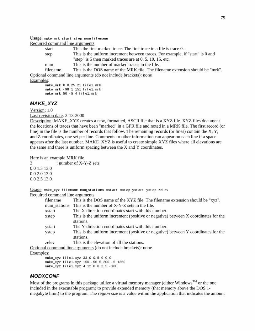
79

Usage: make_mrk start step num filename Required command line arguments:

start This the first marked trace. The first trace in a file is trace 0. step This is the uniform increment between traces. For example, if "start" is 0 and

"step" is 5 then marked traces are at 0, 5, 10, 15, etc. num This is the number of marked traces in the file. filename This is the DOS name of the MRK file. The filename extension should be "mrk".


make_mrk 0 0.25 21 file1.mrk make_mrk -98 1 151 file1.mrk make_mrk 50 -5 4 file1.mrk

MAKE_XYZ Version: 1.0Last revision date: 3-13-2000Description: MAKE_XYZ creates a new, formatted, ASCII file that is a XYZ file. XYZ files documentthe locations of traces that have been "marked" in a GPR file and noted in a MRK file. The first record (orline) in the file is the number of records that follow. The remaining records (or lines) contain the X, Y,and Z coordinates, one set per line. Comments or other information can appear on each line if a spaceappears after the last number. MAKE_XYZ is useful to create simple XYZ files where all elevations arethe same and there is uniform spacing between the X and Y coordinates.

Here is an example MRK file. ; number of X-Y-Z sets

0.0 1.5 13.0 0.0 2.0 13.0 0.0 2.5 13.0

Usage: make_xyz filename num_stations xstart xstep ystart ystep zelev Required command line arguments:

filename This is the DOS name of the XYZ file. The filename extension should be "xyz". num_stations This is the number of X-Y-Z sets in the file. xstart The X-direction coordinates start with this number. xstep This is the uniform increment (positive or negative) between X coordinates for the

stations. ystart The Y-direction coordinates start with this number. ystep This is the uniform increment (positive or negative) between Y coordinates for the

stations. zelev This is the elevation of all the stations.


make_xyz file1.xyz 33 0 0.5 0 0 0 make_xyz file1.xyz 150 -56 5 200 -5 1350 make_xyz file1.xyz 4 12 0 0 2.5 -100

MODXCONF Most of the programs in this package utilize a virtual memory manager (either WindowsTM or the one included in the executable program) to provide extended memory (that memory above the DOS 1-megabyte limit) to the program. The region size is a value within the application that indicates the amount

3

80

of memory the application uses. The utility program MODXCONF is distributed with these programs to modify the region size. MODXCONF is menu-driven. You may need to use this program to change the region size if the GPR application, as distributed, requests more memory than your computer can make available. In this case, you might see some messages like those shown below when you run the GPR application.

DOS Extender: Error X0135: Extended memory exhausted during application loadDOS Extender: Error X0134: Insufficient extended memoryDOS Extender: Error X0130: Failure detected during program load

Be sure that MODXCONF.EXE and MODXCONF.DEX are in the same directory as the target application (or in the directory path) and invoke the utility as shown below.

modxconf filename.exe

Example: modxconf gpr_xsu.exe

Following the menu instructions to change the region size to one that your computer allows and that allows the GPR application to run.

S10_EHDR Version: 1.0Last revision date: 4-23-2001Description: S10_EHDR edits selected field in a DZT file header. The program operates in "batch mode"if the optional command line parameters are given. In batch mode only one of the selected fields can bechanged. In interactive mode (no optional parameters given), a wider selection of fields can be edited.There is an option at the end to save the changes or not. Changes are saved to the input file, not to a newfile.Usage: S10_EHDR dzt_filename [field_number new_value]

Required command line arguments:dzt_filename This is the DOS name of the DZT file that will be edited.

Optional command line arguments (do not include brackets): field_number This is the ID number of the header field that will be changed. new_value This is the new value for the header field

Examples: s10_ehdr file1.dzt s10_ehdr file1.dzt

S10_MRKS Version: 2.0Last revision date: 3-10-2000Description: S10_MRKS finds the marked traces in a DZT file. Four versions of DZT files are accepted:SIR-10 version 5 and later, RADAN, SIR-2, and SIR-2000. Marked traces are identified in these files bysetting the first two samples of each trace to a specific value. The marked trace numbers are listed to thecomputer screen. If the optional MRK filename is given on the command line then the results areautomatically saved to disk. Otherwise, the user is asked if they want to save the results to disk before theapplication ends.Usage: S10_MRKS dzt_filename max_ticks [mrk_filename]

Required command line arguments:dzt_filename This is the DOS name of the DZT file.

81

max_ticks This is the max number of tick you expect to find in the DZT file. This number is used to allocate storage inside the application. Make this number twice the number of tick marks you expect to find. No warning is given if more tick marks are in the file than max_ticks.

Optional command line arguments (do not include brackets): mrk_filename This is the DOS filename of the MRK file that will contain the results of the mark

search. The filename extension is forced to MRK by the application. Examples:

s10_mrks file1.dzt 25 file1 s10_mrks gl1n30.dzt 500

SPECTRA Version: 2.0Last revision date: 4-24-2001Description: SPECTRA is a simple program that takes one trace from a GPR file and displays thefrequency spectrum. Essential values are entered on the DOS command line. An FFT is used to transformthe trace time series data into the frequency domain.Usage: SPECTRA filename file_hdr trace_hdr samp_bytes num_samps num samp_rate [pltfile]

Required command line arguments:filename The DOS filename of the input file.file_hdr The number of bytes in the file header.trace_hdr The number of bytes in the trace header.samp_bytes The number of bytes in each sample. Use 1 for 8-bit data, 2 for 16-bit data, and 4

for 32-bit data. Only integer data can be used. Make this a negative number if the data signed.

num_samps The number of samples in each trace. num The trace number to use from the file. The first trace is trace 0. samp_rate The number of nanoseconds (ns) per sample. The sampling rate.

Optional command line arguments (do not include brackets): pltfile The name of DOS file to store the PLT vector graphics display. This name should

have a filename extension of "plt". Examples:

spectra file1.dzt 1024 0 2 512 95 0.45 spectra file1.dzt 1024 0 2 512 95 0.45 file1.plt spectra line01.dt1 0 128 –2 450 42 0.05 spectra line01.dt1 0 128 –2 760 168 0.025 line01.plt spectra ngrid01.sgy 3600 240 –2 300 4 0.08

SHOWFONT Version: 2.1Last revision date: 1-25-94Description: SHOWFONT displays in graphics mode the 256 characters available for one of the Hersheyfonts provided with this software. This program must be run in the "hershey" folder or directory.SHOWFONT was supplied with the graphics library used by these programs and was not written by theauthors or this report.Usage: SHOWFONT fontnameRequired command line arguments:

fontname The 8-character name of the Hershey font. Type the name of the program without a font name and a list of available fonts are listed.


showfont cyrillic

82

showfont romtrplx

Libraries Description The source code for the utility libraries is provided to benefit application developers and to assist end users in understanding how particular functions are implemented.

GPR_DFX The functions in this library perform operations on GPR single traces or groups of traces.

The following functions are included in GPR_DFX.LIB AdjustMeanGridTraces Add a constant value to all samples in a trace, so that the trace mean

value is changed. ApplyGridSpatMedFilter Apply a median filter to the rows of samples (that is, across the traces) in

a grid of traces. ApplyGridTempMedFilter Apply a median filter to the columns of samples (that is, along one trace)

in a grid of traces. ChangeGridRangeGain Change the range gain of all traces in a grid of traces. EqualizeGridTraces Multiply each sample in each trace in the grid of traces by a constant

value so that the sum of all sample amplitudes (about 0) is the same as the sum for the base_trace.

FftFilterGridTraces Transform all traces in a grid of traces into their frequency domain. InstAttribGridTraces Transform all sample in a trace into instantaneous amplitude or

instantaneous power. RemGridGlobBckgrnd Remove a background trace (the average trace of all traces) from every

trace in a grid of traces. RemGridGlobForgrnd Assign the background trace (the average trace of all traces) to every

trace in a grid of traces. RemGridWindBckgrnd Remove a running window background trace (the average of a few

traces) from every trace in a grid of traces. RemGridWindForgrnd Assign the running window background trace (the average of a few

traces) to every trace in a grid of traces. RescaleGrid Multiply each sample in each trace in a grid of traces by a constant value. SlideSamples Slide each sample value up or down in each trace in a grid of traces. SmoothGridHorizontally Smooth all the traces in a grid of traces "horizontally" by sliding a

window through the grid and averaging the traces within the window using a Hanning function (0.5 - 0.5 * cos(t)), where the middle trace has a weight of 1 and the traces at either end of the window have weights of 0. The weighted-average trace is then assigned to the trace in the grid.

SmoothGridVertically Smooth the data "vertically" by sliding a window through each trace in a grid of traces and averaging the samples within the window using a Hanning function (0.5 - 0.5 * cos(t)), where the middle sample has a weight of 1 and the samples at either end of the window have weights of 0. The weighted-average sample is then assigned to the trace in the grid.

StackGrid Stack the specified number of traces in the grid into a new average trace. The number of grid columns (traces) is reduced and columns no longer need in the grid are freed.

GPR_IFX The functions in this library manipulate a lookup table that maps the 8-bit values in an image. The image must be an 8-bit "gray-scale" image.

83

The following functions are included in GPR_IFX.LIBBrightenTable8 Add a constant value to all table entries.InitTable8 Initialize the table for either gray scale or EPC style.LocalStretchTable8 Enhance the contrast locally in the table.ReverseTable8 Reverse the order of values in the table.SquareTable8 Square the values in the table then re-scales them to 8-bit range.

GPR_IO Four source files contain the functions that are in this library. These functions handle data input andoutput (I/O) to and from disk.

These functions handle Sensors & Software DT1/HD files.GetSsHdFileGetSsTraceInitDt1ParametersPrintSsHdInfoPrintSsTraceHdrSaveSsHdFileSetDt1TraceHeader

These functions handle GSSI DZT files.ConvertProcHist2EditDztHeaderGetDztChSubGrid8GetDztChSubGrid16GetDztChSubImage8GetDztFilePrintOneDztHeaderReadOneDztHeaderSaveDztFileSetDztHeaderSetDzt5xHeader

These are general functions related to GPR file I/O.ExtractSsInfoFromSegyGetGprFileTypeGetGprSubGridGetMrkDataGetSubImage8GetXyzDataInitGprInfoStruct

These functions handle SEG-Y files.GetSegyReelHdrGetSegyTracePrintSegyReelHdrPrintSegyTraceHdrPrintSuTraceHdrReadSegyReelHdr

84

SetSgyFileHeader SetSgyTraceHeader SetSuTraceHeader

JL_UTIL1 These functions provide utility operations used in a multitude of applications.

The following functions are included in JL_UTIL1.LIB.ANSI_there Tests to see if ANSI.SYS is loaded.BandPassFFT1D Performs a bandpass frequency filter of a time series.CreateDir Creates a DOS directory at any allowed level.FftFilterTrace Performs high/low frequency filter of a time series.FFT1D Performs a standard FFT/IFFT of a time series.GetDosVersion Reports DOS version (old style).InstAttribTrace Calculates instantaneous amplitude or instantaneous power of a time

series. LinFit Calculates the least-squares fit to data with a straight line. RealFFT1D Performs a "packed" FFT of a real function. Sound Generates a sound using the PC speaker. Spline Performs a cubic spline interpolation of a data set. Spline2 Performs a cubic spline interpolation allowing interpolation outside of

the ends. TrimStr Removes blank and unprintable characters from the beginning and end of

a string. The remaining characters are slid up to the starting pointer.

PCX_IO These functions perform the basic operations needed to create PCX graphics files of the GPR screenimages.

The following functions are included in PCX_IO.LIB.PcxDecodeScanLinePcxEncodeScanLineSetPcxHeader

Examples The Examples folder contains command files for the program GPR_DISP. In a DOS "window", type in the following and press <Enter>: gpr_disp tstdisp1.cmd. The screen will go blank for a little while six GPR_DISP command files are being executed. An image will then appear presenting radar data in six different visual formats. For a hardcopy of the screen image, edit the file tstdisp1.cmd and add an equal sign after the keyword eps_outfilename. Look at the CMD files carefully to determine how to produce the radar images you see on the screen.

References Cohen, J.K and Stockwell, Jr., J.W., 1999, CWP/SU – Seismic Unix Release 33 – A free package for

seismic research and processing: Center for Wave Phenomenon, Colorado School of Mines, Available at ftp.cwp.mines.edu (138.67.12.4).

K. M. Barry, D. A. Cavers, C. W. Kneale, 1975, Recommended Standards for Digital Tape Formats: Geophysics, v. 40, p.344-352.

ftp://ftp.cwp.mines.edu/

85

Yilmaz, Ozdogan, 1987, Seismic Data Processing, Society of Exploration Geophysicists: Tulsa, OK, USA, 526 p.

Appendix A - GPR Data Storage Formats The most commonly encountered GPR storage formats are described below. Here is a summary of the basic file structures.

Make Data File channels file header trace header samples

bytes bytes GSSI up to 4 1024/ch 0 power of 2

128 to 2048 S&S 1 0 128 variable Malå 1 0 0 variable SEGY 1 3600 240 variable

GSSI - DZT

Info file bytes/sample

8 or 16 no unsigned

16 signed yes 16 signed yes 8 or 16 signed no 32 float

The equipment manufacturer is Geophysical Survey Systems, Inc. They are located at 13 Klein Drive, North Salem, NH 03073, USA (telephone: 603-893-1109). Their web site is http://www.geophysical.com/ .

A GSSI SIR-10 binary data file consists of a file header section at the start of the file followed by the GPR traces in the data section. Each file can have from 1 to 4 data channels. file headers:

- from 1 to 4, each being 1024 bytes (current versions) or 512 bytes (older versions). - each header is a "C" language structure packed on byte boundaries. - older versions may not perform and record a checksum.

data: - traces do not have individual headers, as such. - traces consist of 128, 256, 512, 1024, or 2048 samples. - samples are 8-bit (1-byte) or 16-bit (2-byte) unsigned integers. - traces are grouped together as blocks in multi-channel files like (for example, a 4-channel file):

trace 0 chan 0, trace 0 chan 1, trace 0 chan 2, trace 0 chan 3, trace 1 chan 0, trace 1 chan 1, trace 1 chan 2, trace 1 chan 3, trace 2 chan 0, etc.

- trace blocks have the first 2 samples of the channel 0 trace reserved (the same is true for single channel files):

- The first byte of the first sample usually has all bits set: 0xFF or 0xFFF. In some version 4.x software, only the high bit is set, 0x80 or 0x8000, for normal traces and all set 0xFF 0r 0xFFFF for marker traces. In version 5.1 beta, the high bit is the only one not set, 0x7F. The second byte (16-bit data) may be set to 0x00 or 0xFF. In version 5.2 beta (last one I know of and the in our SIR-10A+) always has all bits set for the first sample, 0xFF or 0xFFFF.

- The second sample is usually set to 0xF1 or 0xF100, 0xF0 or 0xF000, or 0x80 or 0x8000, for non-marker traces. If a marker occurs at a trace (marker button was pressed on the control unit or at the antenna) then the second sample is set to 0xE8 or 0xE800, 0xE1 or 0xE100, 0xEC or 0xEC00, (or even 0xF1 or 0xF100 for some version 4.x software where normal traces are 0x80 or 0x8000).

- the first and second samples of channels 1, 2, and 3, for multi-channel files, are not reserved.

86

Here are the combinations I have observed for 16-bit data sets, in hexadecimal notation. Normal trace Marker trace

SIR-10 Version First sample Second sample First sample Second sample 3.x FF00 F000 FF00 EC00 4.x FFFF F100 FFFF E100 4.x 8000 8000 FFFF F100 5.0 beta FFFF F100 FFFF E800 5.1 beta 7FFF F000 7FFF E800 5.2 beta FFFF F000 FFFF E800

For 8-bit data, just use the first byte (for example, FF instead FF00, or EC instead of EC00).

This lack of consistency makes it difficult to differentiate normal traces from marker traces automatically. The data must be inspected first to determine GSSI's scheme for setting the first 2 samples of the traces of the first channel. Since markers usually only cover one or a few traces, many traces could be checked and a statistical method used to determine the scheme. The program GPR_RHDR can display the first 2 samples of GSSI data after displaying the header information.

The two structures used in the DZT file header are listed in Appendix A.

Sensors & Software – DT1/HD The equipment manufacturer is Sensors & Software, Inc. They are located at 1091 Brevik Place, Mississauga, Ontario L4W 3R7, Canada (telephone: 800-267-6013, 905-624-8909) Their web site is http://www.sensoft.on.ca/ .

The pulseEKKO GPR systems store the radar traces in binary format in a file with a "DT1" filename extension and information about the traces in an ASCII file with a "HD" extension. Both files have the same 8-character filename.

The header file, the HD file, has keywords in it that specify information about the radar data, such as number of samples and traces, time window, etc., and can be variable in length. Any DOS text editor can look at or modify them. An example is shown below:

8000Fracture Mapping In Rock21/09/89 NUMBER OF TRACESNUMBER OF PTS/TRC TIMEZERO AT POINT TOTAL TIME WINDOW STARTING POSITION FINAL POSITIONSTEP SIZE USEDPOSITION UNITSNOMINAL FREQUENCY ANTENNA SEPARATION PULSER VOLTAGE (V) NUMBER OF STACKSSURVEY MODE

= 136 = 409 = 96 = 327 = 9.500000 = 77.000000 = 0.500000 = metres = 100.000000 = 1.000000 = 400 = 128 = Reflection

123456789

87

The data file is written in binary format and contains a record for every trace. Each record consists of a 128-byte header section and a data section. The header section consists of an array of 25 4-byte reals, or floating point numbers, and a string of 28 characters (that take the same storage space as 7 4-byte reals). The data section consists of an array of 2-byte signed integers, one integer for every data sample point. The number of sample points is variable and does not have to be a power of 2. The 32 element real array contains the following information:

Item # Description

Trace numberPositionNumber of points per traceTopographic data, if available(not used)# bytes/point (always 2 for Rev 3 firmware)Trace Number# of stacksTime window

10-14 Not used 15 Reserved for receiver x position 16 Reserved for receiver y position 17 Reserved for receiver z position 18 Reserved for transmitter x position 19 Reserved for transmitter y position 20 Reserved for transmitter z position 21 time zero adjustment

where: point(x) = point(x + adjustment) 22 Zero flag: 0 = data okay, 1=zero data 23 (not used) 24 Time of day data collected in seconds past midnight. 25 Comment flag: 1 = comment attached. 26-32 Comment

The trace header structure is listed in Appendix B.

SEG – SEG-Y The reference for the SEG-Y standard is K. M. Barry and others (1975).

The SEG-Y file format is as follows: <Reel Identification Header> <Trace Data Block 1> <Trace Data Block 2>

... ... ... <Trace Data Block N>

The SEG-Y file format is the standardized data storage for seismic magnetic reel tapes. It can be generally described as follows.

1. A reel identification header consisting of 3600 bytes in 2 parts: - 3200 (0xC80) bytes of EBCDIC characters representing 40 80-byte

"card images", and

88

- 400 (0x190) bytes of binary fixed-point integers, the first 60 bytes are assigned, the remaining 340 bytes are unassigned for optional use;

2. A trace data block consisting of a trace ID header and the trace data: - 240 (0xF0) bytes in trace identification header consisting of binary

fixed-point and floating-point numbers, and - the trace data samples (number, length, and type defined in the reel

ID header); and 3. More trace data blocks.

Fixed-point values must be either 16 bits or 32 bits in two's complement notation. Positive values are true binary numbers (highest bit must never be set, though). Negative values are obtained by inverting each bit of the positive binary number and adding one (1) to the least significant bit position (highest bit is always set).

Floating-point values must be 32 bits in IBM-compatible floating-point notation (as defined in IBM Form GA 22-6821). Mainframe computers almost universally use this format. Microcomputers, such as those using the Intel 80x86 family of processors, almost universally use IEEE floating point format.

The SEG-Y byte-ordering convention stores the most significant byte (MSB), high byte, first and the least significant byte (LSB), low byte, last. This big-endian convention is typical of the Motorola 86000 family of processor chips, but reverse of the order from the Intel 80x86 family of processors (little-endian). For example, the number 15, if stored as a 2-byte fixed-point number, would be represented in hexadecimal by the I80x86 processor as 0F 00, and by the M86000 processor as 00 0F.

The functions used here will read all SEG-Y files if they follow the format described above with two exceptions; only IEEE floating point format will be recognized and character codes will be interpreted as ASCII assignments. Inspecting the values in the format member of the reel ID header recognizes the byte ordering. SEG-Y files written by these functions will use IEEE floating point format and the ASCII character codes; byte ordering can be specified for saving files; it is automatically converted to Intel littleendian style if necessary when reading files.

The SEG-Y reel identification and trace header structures are listed in Appendix A.

RAMAC – RD3/RAD The equipment manufacturer is Malå GeoScience. They are located at Skolgatan 11, S-930 70 Malå, Sweden. Their USA office is Malå GeoScience USA, Inc., P.O. Box 80430, Charleston, SC 29416 (telephone: 843-852-5021). Their web site is http://www.malags.se/ .

The RAMAC GPR systems store the radar traces in binary format in a file with a "RD3" filename extension and information about the traces in an ASCII file with a "RAD" extension. Both files have the same 8-character filename.

The header file, the RAD file, has keywords in it that specify information about the radar data, such as number of samples and traces, time window, etc., and can be variable in length. Any DOS text editor can look at or modify them. An example is shown below:

SAMPLES:512FREQUENCY:4871.373810FREQUENCY STEPS:1SIGNAL POSITION:-0.002258

89

RAW SIGNAL POSITION:32778DISTANCE FLAG:1TIME FLAG:0PROGRAM FLAG:0EXTERNAL FLAG:0TIME INTERVAL:0.010000DISTANCE INTERVAL:0.030000OPERATOR:CUSTOMER:ESSESITE:ANTENNAS:400ANTENNA ORIENTATION:normalANTENNA SEPARATION:0.600000COMMENT:TIMEWINDOW:0.105104STACKS:32STACK EXPONENT:5STACKING TIME:0.163840LAST TRACE:532STOP POSITION:16.06SYSTEM CALIBRATION:0.0002052809

The data file is written in binary format and contains a record for every trace. Each record consists only of a data section. There is no trace header. The data section consists of an array of 2-byte signed integers, one integer for every data sample point. The number of sample points is variable and does not have to be a power of 2.

Seismic Unix – SU The SU storage format is used only in the Seismic Unix (SU) programs (Cohen and Stockwell, 1999). It is not associated with any GPR manufacturer. There is a binary data file with no file header and one record for every trace. Each record consists of a 240-byte header section and a data section. The trace header is similar in structure to the SEG-Y trace header. The data section consists of an array of 2-byte signed integers, one integer for every data sample point. Floating point values can also be used. The number of sample points is variable and does not have to be a power of 2.

Appendix B – GPR Data Structures

GSSI - DZT

Here are the two structures used in the DZT file header.

struct DztDateStruct { unsigned sec2 : 5; /* second/2 (0-29) */

unsigned min : 6; /* minute (0-59) */ unsigned hour : 5; /* hour (0-23) */ unsigned day : 5; /* day (1-31) */ unsigned month : 4; /* month (1-12; 1=Jan, 2=Feb, etc. */ unsigned year : 7; /* year-1980 (0-127; 1980-2107) */

} ; /* 4 bytes (32 bits) if tightly packed */

/* Note: the following structure incorporates the changes noted in the

90

* preliminary draft for extended RADAN file header format as * faxed to Jeff Lucius by Leo Galinovsky (GSSI) 1/11/94. */ struct DztHdrStruct { unsigned short rh_tag;

unsigned short rh_data; unsigned short rh_nsamp; unsigned short rh_bits; short rh_zero; float rh_sps; float rh_spm; float rh_mpm; float rh_position; float rh_range; unsigned short rh_npass; struct DztDateStruct rh_create; struct DztDateStruct rh_modif; unsigned short rh_rgain; unsigned short rh_nrgain; unsigned short rh_text; unsigned short rh_ntext; unsigned short rh_proc; unsigned short rh_nproc; unsigned short rh_nchan; float rh_epsr; float rh_top; float rh_depth;

/* 0x0Nff, where N = rh_nchan-1 (0 - 15) *//* offset to data (1024 * rh_nchan) *//* samples per scan (2 - 65535) *//* bits per data word (8, 16, 32, 64) *//* binary offset (-128, -32768, etc.) *//* scans per second *//* scans per meter *//* meters per mark *//* position (ns) *//* range (ns) *//* scans per pass for 2D files *//* date created *//* date modified *//* offset to range gain function *//* size of range gain function *//* offset to text *//* size of text *//* offset to processing history *//* size of processing history *//* number of channels *//* average dielectric constant *//* top position in meters *//* range in meters */

char reserved[31]; char rh_dtype;

/* bits: 7 6 5 4 3 2 1 0 0 unsigned data 1 signed data

0 8-bit int 1 16-bit int

1 32-bit int 1 64-bit int

1 32-bit float 1 64-bit float (USGS extn.)

X X X not used /* rh_dtype does not appear in versions before 5.2 */

char rh_antname[14]; /* antenna name (eg. 3105(300 MHz)) */ unsigned short rh_chanmask; /* active channels mask

format is 0x530X, where X has following bits set: bits: 7 6 5 4 3 2 1 0

1 1 channel 1 1 2 channels

1 1 1 3 channels1 1 1 1 4 channels

0 0 0 0 not used*/

char rh_name[12]; /* this filename without DOS extension */ unsigned short rh_chksum; /* checksum for header; NOTE: see program

below for proper way to calculate header checksum (essentially, zero out old checksum value (copy it first) and add up values in the header as if it were 512 unsigned shorts, then place checksum value into rh_chksum. */

/* 128 bytes to here */char variable[896]; /* range gain, comments, and processing

history */ } ; /* 1024 bytes if tightly packed */ /* * WARNING! In older DZT files, the rh_data field may not actually be the * offset to data in multi-channel files! It is probably best to * read in all the headers which leaves the file pointer at the

---------------------

91

* start of the first scan or read in the first header to * discover the number of channels then rewind the file and move * the file pointer "number of channels times sizeof(the header * structure)". */

Here is a function that prints out the contents of a DZT file header. It also shows how the checksum is calculated and how to read the range gain.

/*************************** PrintOneDztHeader() ***************************/ /* Print out the contents of one DZT file header to an output device * (stdout, stderr, a disk file, etc.).. * * Parameters: * int header_bytes - number of actual bytes in file header, 512 or 1024 * int num_traces - number of radar scans, <=0 if unknown * char *out_filename - "stdout", "stderr", or a DOS filename * char *dzt_filename - DOS name of the DZT file header(s) belong to * struct DztHdrStruct *hdrPtr1 - addresses of the header * * Requires: <conio.h>, <stdio.h>, <string.h>, "gpr_io.h". * Calls: fopen, fprintf, getch, strstr, ConvertProcHist2. * Returns: 0 on success, * >0 on error (offset into an array of strings). * * Author: Jeff Lucius USGS Branch of Geophysics Golden, CO * Date: December 1, 1995 */ int PrintOneDztHeader (int header_bytes,long num_traces,char *out_filename,

char *dzt_filename,struct DztHdrStruct *hdrPtr) {

char ant_freq[10],newstr[32]; unsigned short rg_breaks = 0; unsigned short checksum; unsigned short ustemp; int i,rg_break_delta; FILE *stream = NULL;

static char big_buff[1024]; /* removes from stack and places in data segment */

extern const char *ant_number[]; /* in "dzt_io.h" */ extern const char *ant_name[]; /* in "dzt_io.h" */ extern const char *month_abbr[]; /* in "dzt_io.h" */

/* Assign or open stream */if (strstr(out_filename,"stdout")) stream = stdout;else if (strstr(out_filename,"stderr")) stream = stderr;else stream = fopen(out_filename,"wt");if (stream == NULL) return 1;

/* Print the header information */fprintf(stream,"SIR-10A header for file %s:\n",dzt_filename);fprintf(stream,"number of headers = %d\n",hdrPtr->rh_nchan);fprintf(stream,"file header size = %d\n",header_bytes);if (num_traces > 0)

fprintf(stream,"number of GPR traces = %d\n",num_traces); fprintf(stream,"SIR-10A header ID = 0x%04x\n",hdrPtr->rh_tag); fprintf(stream,"offset to data = %hd\n",hdrPtr->rh_data); fprintf(stream,"samples per scan = %hu\n",hdrPtr->rh_nsamp); fprintf(stream,"bits per data word = %hu\n",hdrPtr->rh_bits); fprintf(stream,"binary offset = %hd (0x%04X)\n",

hdrPtr->rh_zero,(unsigned short)hdrPtr->rh_zero); fprintf(stream,"scans per second = %f\n",hdrPtr->rh_sps);

92

fprintf(stream,"scans per meter = %f\n",hdrPtr->rh_spm); fprintf(stream,"meters per mark = %f\n",hdrPtr->rh_mpm); fprintf(stream,"position (ns) = %f\n",hdrPtr->rh_position); fprintf(stream,"range (ns) = %f\n",hdrPtr->rh_range); fprintf(stream,"scans per pass = %hu\n",hdrPtr->rh_npass); if (hdrPtr->rh_create.month == 0)

fprintf(stream,"create date = no date\n"); else

fprintf(stream,"create date = %s %d, %d (%d:%02d:%02d)\n", month_abbr[hdrPtr->rh_create.month],hdrPtr->rh_create.day, hdrPtr->rh_create.year+1980, hdrPtr->rh_create.hour, hdrPtr->rh_create.min, hdrPtr->rh_create.sec2*2);

if (hdrPtr->rh_modif.month == 0) fprintf(stream,"modification date = no date\n");

else fprintf(stream,"modification date = %s %d, %d (%d:%02d:%02d)\n",

month_abbr[hdrPtr->rh_modif.month],hdrPtr->rh_modif.day, hdrPtr->rh_modif.year+1980, hdrPtr->rh_modif.hour,hdrPtr->rh_modif.min, hdrPtr->rh_modif.sec2*2);

fprintf(stream,"offset to range gain = %hu\n",hdrPtr->rh_rgain);fprintf(stream,"size of range gain = %hu\n",hdrPtr->rh_nrgain);fprintf(stream,"offset to text = %hu\n",hdrPtr->rh_text);fprintf(stream,"size of text = %hu\n",hdrPtr->rh_ntext);fprintf(stream,"offset to proc.hist. = %hu\n",hdrPtr->rh_proc);fprintf(stream,"size of proc.hist. = %hu\n",hdrPtr->rh_nproc);if (stream==stdout || stream==stderr){ fprintf(stream,"Press a key to continue ...");

getch();/* fprintf(stream,"\r \r");*/puts("");

}fprintf(stream,"number of channels = %hu\n",hdrPtr->rh_nchan);fprintf(stream,"ave. diel. constant = %f\n",hdrPtr->rh_epsr);fprintf(stream,"top pos. in meters = %f\n",hdrPtr->rh_top);fprintf(stream,"range in meters = %f\n",hdrPtr->rh_depth);fprintf(stream,"reserved = %s\n",hdrPtr->reserved);ant_freq[0] = 0;for (i=0; ant_number[i]; i++){ if (strstr(hdrPtr->rh_antname,ant_number[i]))

{ strcpy(ant_freq,ant_name[i]); break; /* out of for loop */

} } fprintf(stream,"antenna name = %s",hdrPtr->rh_antname); if (ant_freq[0]) fprintf(stream," (%s)",ant_freq); fprintf(stream,"\n"); fprintf(stream,"active channels mask = 0x%04X\n",hdrPtr->rh_chanmask); fprintf(stream,"this file name = %s\n",hdrPtr->rh_name);

/* Calculate checksum for header */if (hdrPtr->rh_chksum != 0){ fprintf(stream,"checksum for header = %hu (0x%04X)\n",

hdrPtr->rh_chksum, hdrPtr->rh_chksum); ustemp = hdrPtr->rh_chksum; hdrPtr->rh_chksum = 0; checksum = 0; for (i=0; i<512; i++)

checksum += *((unsigned short *)hdrPtr + i); fprintf(stream,"calculated checksum = %hu (0x%04X) [header %s corrupted]\n",

checksum,checksum,(checksum==ustemp) ? "is not" : "is"); hdrPtr->rh_chksum = ustemp;

93

}if (hdrPtr->rh_rgain != 0 && hdrPtr->rh_nrgain != 0){ rg_breaks = *(unsigned short *) ((char *)hdrPtr + hdrPtr->rh_rgain);

fprintf(stream,"number of rg breaks = %hd\n",rg_breaks);fprintf(stream,"range gain: scan sample db\n");rg_break_delta = (hdrPtr->rh_nsamp-1) / (rg_breaks-1);for (i=0; i<rg_breaks; i++){ fprintf(stream," %3d %7.3f\n",

rg_break_delta*i,*(float *)((char *)hdrPtr + hdrPtr->rh_rgain + 2 + 4*i));

} } if (stream==stdout || stream==stderr) { fprintf(stream,"Press a key to continue ...");

getch();/* fprintf(stream,"\r \r");*/puts("");

} if (hdrPtr->rh_text)

fprintf(stream,"comments =\n%s\n",(char *)hdrPtr + hdrPtr->rh_text); else

fprintf(stream,"no comments\n"); if (hdrPtr->rh_nproc)

Note: The source code for ConvertProcHist2() is in the file DZT_IO.C

{ ConvertProcHist2((int)sizeof(big_buff),big_buff,( int)hdrPtr->rh_nproc, ((char *)hdrPtr + hdrPtr->rh_proc));

fprintf(stream,"Processing History:\n"); if (strlen(big_buff)) fprintf(stream,"%s\n",big_buff); else fprintf(stream,"\tnone\n\n");

} else

fprintf(stream,"no processing history\n"); if (strstr(out_filename,"stdout")) ; else if (strstr(out_filename,"stderr")) ; else fclose(stream); return 0;

}

Sensors & Software – DT1/HD

/* This structure is present before every trace in the *.DT1 data file */struct SsTraceHdrStruct{ /* trace identification header */

float trace_num; /* trace sequence number within line */float position; /* position along traverse */float num_samples; /* samples per trace */float elevation; /* elevation data if available */float unass5; /* unassigned */float num_bytes; /* bytes per sample; always 2 for Rev. 3 firmware */float aux_trace_num; /* trace number again */float num_stacks; /* number of stacks used to get trace */float time_window; /* time window in ns */float unass10; /* unassigned */float unass11; /* unassigned */float unass12; /* unassigned */float unass13; /* unassigned */float unass14; /* unassigned */float unass15; /* unassigned */float unass16; /* unassigned */

94

float unass17; /* unassigned */float unass18; /* unassigned */float unass19; /* unassigned */float unass20; /* unassigned */float time_zero_adjust; /* where sample x = sample x + adjustment */float zero_flag; /* 0 = data OK, 1 = zero data */float unass23; /* unassigned */float time; /* seconds past midnight */float comment_flag; /* 1 = comment attached */char comment[28]; /* optional character comments */

} ; /* 128 bytes if tightly packed */

SEG – SEGY

/* the SEG-Y reel identification header */struct SegyReelHdrStruct{ /* ASCII- or EBCDIC-coded block */

char comment[3200]; /* 3200-byte text area */ /* binary-coded block */ long int jobid; /* job identification number */ long int lino; /* line number (only one line per reel) */ long int reno; /* reel number */ short int ntrpr; /* number of data traces per record */ short int nart; /* number of auxiliary traces per record */ short int hdt; /* sample interval in micro secs for this reel */ short int dto; /* same for original field recording */ short int hns; /* number of samples per trace for this reel */ short int nso; /* number of samples per trace for original field recording */ short int format; /* data sample format code:

1 = floating point (4 bytes)2 = fixed point (4 bytes)3 = fixed point (2 bytes)4 = fixed point w/gain code (4 bytes) */

short int fold; /* CDP fold expected per CDP ensemble */ short int tsort; /* trace sorting code:

1 = as recorded (no sorting) 2 = CDP ensemble 3 = single fold continuous profile 4 = horizontally stacked */

short int vscode; /* vertical sum code: 1 = no sum 2 = two sum ... N = N sum (N = 32,767) */

short int hsfs; /* sweep frequency at start */ short int hsfe; /* sweep frequency at end */ short int hslen; /* sweep length (ms) */ short int hstyp; /* sweep type code:

1 = linear 2 = parabolic 3 = exponential 4 = other */

short int schn; /* trace number of sweep channel */ short int hstas; /* sweep trace taper length (msec) at start if

tapered (the taper starts at zero time and is effective for this length) */

short int hstae; /* sweep trace taper length (msec) at end (the ending taper starts at sweep length minus the taper length at end) */

short int htatyp; /* sweep trace taper type code: 1 = linear 2 = cos-squared 3 = other */

short int hcorr; /* correlated data traces code:

1 2 3 4 5 6 7 8

95

1 = no 2 = yes */

short int bgrcv; /* binary gain recovered code: 1 = yes 2 = no */

short int rcvm; /* amplitude recovery method code: 1 = none 2 = spherical divergence 3 = AGC 4 = other */

short int mfeet; /* measurement system code: 1 = meters 2 = feet */

short int polyt; /* impulse signal polarity code: 1 = increase in pressure or upward

geophone case movement gives negative number on tape

2 = increase in pressure or upward geophone case movement gives positive number on tape */

short int vpol; /* vibratory polarity code: code seismic signal lags pilot by

337.5 to 22.5 degrees 22.5 to 67.5 degrees 67.5 to 112.5 degrees 112.5 to 157.5 degrees 157.5 to 202.5 degrees 202.5 to 247.5 degrees 247.5 to 292.5 degrees 293.5 to 337.5 degrees */

short int hunass[170]; /* unassigned */ } ; /* 3600 bytes if tightly packed */

/* the SEG-Y trace identification header */ struct SegyTraceHdrStruct { long int tracl; /* trace sequence number within line */

long int tracr; /* trace sequence number within reel */long int fldr; /* field record number */long int tracf; /* trace number within field record */long int ep; /* energy source point number */long int cdp; /* CDP ensemble number */long int cdpt; /* trace number within CDP ensemble */short int trid; /* trace identification code:

1 = seismic data2 = dead3 = dummy4 = time break5 = uphole6 = sweep7 = timing8 = water break9---, N = optional use (N = 32,767)Following are CWP id flags:9 = autocorrelation10 = Fourier transformed - no packing

xr[0],xi[0], ..., xr[N-1],xi[N-1] 11 = Fourier transformed - unpacked Nyquist

xr[0],xi[0],...,xr[N/2],xi[N/2] 12 = Fourier transformed - packed Nyquist

even N: xr[0],xr[N/2],xr[1],xi[1], ...,

xr[N/2 -1],xi[N/2 -1] (note the exceptional second entry) odd N:

96

xr[0],xr[(N-1)/2],xr[1],xi[1], ..., xr[(N-1)/2 -1],xi[(N-1)/2 -1], xi[(N-1)/2]

(note the exceptional second & last entries) 13 = Complex signal in the time domain

xr[0],xi[0], ..., xr[N-1],xi[N-1] 14 = Fourier transformed - amplitude/phase

a[0],p[0], ..., a[N-1],p[N-1] 15 = Complex time signal - amplitude/phase

a[0],p[0], ..., a[N-1],p[N-1] 16 = Real part of complex trace from 0 to Nyquist 17 = Imag part of complex trace from 0 to Nyquist 18 = Amplitude of complex trace from 0 to Nyquist

19 = Phase of complex trace from 0 to Nyquist 21 = Wavenumber time domain (k-t) 22 = Wavenumber frequency (k-omega) 30 = Depth-Range (z-x) traces

101 = Seismic data packed to bytes (by supack1) 102 = Seismic data packed to 2 bytes (by supack2) 200 = GPR data

*/ short int nvs; /* number of vertically summed traces (see vscode

in reel header structure) */ short int nhs; /* number of horizontally summed traces (see vscode

in reel header structure) */ short int duse; /* data use:

1 = production 2 = test */

long int offset; /* distance from source point to receiver group (negative if opposite to direction in which the line was shot) */

long int gelev; /* receiver group elevation from sea level (above sea level is positive) */

long int selev; /* source elevation from sea level (above sea level is positive) */

long int sdepth; /* source depth below surface (positive) */ long int gdel; /* datum elevation at receiver group */ long int sdel; /* datum elevation at source */ long int swdep; /* water depth at source */ long int gwdep; /* water depth at receiver group */ short int scalel; /* scale factor for previous 7 entries

with value plus or minus 10 to the power 0, 1, 2, 3, or 4 (if positive, multiply, if negative divide) */

short int scalco; /* scale factor for next 4 entries with value plus or minus 10 to the power 0, 1, 2, 3, or 4 (if positive, multiply, if negative divide) */

long int sx; /* X source coordinate */ long int sy; /* Y source coordinate */ long int gx; /* X group coordinate */ long int gy; /* Y group coordinate */ short int counit; /* coordinate units code:

for previous four entries1 = length (meters or feet)2 = seconds of arc (in this case, theX values are longitude and the Y valuesare latitude, a positive value designatesthe number of seconds east of Greenwichor north of the equator */

short int wevel; /* weathering velocity */

97

short int swevel; /* subweathering velocity */ short int sut; /* uphole time at source */ short int gut; /* uphole time at receiver group */ short int sstat; /* source static correction */ short int gstat; /* group static correction */ short int tstat; /* total static applied */ short int laga; /* lag time A, time in ms between end of 240-

byte trace identification header and time break, positive if time break occurs after end of header, time break is defined as the initiation pulse which maybe recorded on an auxiliary trace or as otherwise specified by the recording system */

short int lagb; /* lag time B, time in ms between the time break and the initiation time of the energy source, may be positive or negative */

short int delrt; /* delay recording time, time in ms between initiation time of energy source and time when recording of data samples begins (for deep water work if recording does not start at zero time) */

short int muts; /* mute time--start */short int mute; /* mute time--end */unsigned short int ns; /* number of samples in this trace */unsigned short int dt; /* sample interval; in micro-seconds */short int gain; /* gain type of field instruments code:

1 = fixed2 = binary3 = floating point4 ---- N = optional use */

short int igc; /* instrument gain constant */ short int igi; /* instrument early or initial gain */ short int corr; /* correlated:

1 = no 2 = yes */

short int sfs; /* sweep frequency at start */ short int sfe; /* sweep frequency at end */ short int slen; /* sweep length in ms */ short int styp; /* sweep type code:


short int stas; /* sweep trace taper length at start in ms */ short int stae; /* sweep trace taper length at end in ms */ short int tatyp; /* taper type: 1=linear, 2=cos^2, 3=other */ short int afilf; /* alias filter frequency if used */ short int afils; /* alias filter slope */ short int nofilf; /* notch filter frequency if used */ short int nofils; /* notch filter slope */ short int lcf; /* low cut frequency if used */ short int hcf; /* high cut frequncy if used */ short int lcs; /* low cut slope */ short int hcs; /* high cut slope */ short int year; /* year data recorded */ short int day; /* day of year */ short int hour; /* hour of day (24 hour clock) */ short int minute; /* minute of hour */ short int sec; /* second of minute */ short int timbas; /* time basis code:

1 = local 2 = GMT 3 = other */

short int trwf; /* trace weighting factor, defined as 1/2^N

98

volts for the least sigificant bit */ short int grnors; /* geophone group number of roll switch

position one */ short int grnofr; /* geophone group number of trace one within

original field record */ short int grnlof; /* geophone group number of last trace within

original field record */ short int gaps; /* gap size (total number of groups dropped) */ short int otrav; /* overtravel taper code:

1 = down (or behind) 2 = up (or ahead) */

short int unass[30]; /* unassigned -- for optional info */ #if 0

/* local assignments, su version of segy headers */ float d1; /* sample spacing for non-seismic data */ float f1; /* first sample location for non-seismic data */ float d2; /* sample spacing between traces */ float f2; /* first trace location */ float ungpow; /* negative of power used for dynamic

range compression */ float unscale; /* reciprocal of scaling factor to normalize range */ short int mark; /* mark selected traces */ short int unass[17]; /* unassigned--NOTE: last entry causes

a break in the word alignment, if we REALLY want to maintain 240 bytes, the following entry should be an odd number of short/UINT2 OR do the insertion above the "mark" keyword entry */

#endif} ; /* 240 bytes if tightly packed */

Seismic Unix – SU

/* the SU trace identification header */#define SU_NFLTS 32768 /* Arbitrary limit on data array size */struct SuTraceHdrStruct{ long int tracl; /* trace sequence number within line */

long int tracr; /* trace sequence number within reel */long int fldr; /* field record number */long int tracf; /* trace number within field record */long int ep; /* energy source point number */long int cdp; /* CDP ensemble number */long int cdpt; /* trace number within CDP ensemble */short int trid; /* trace identification code:

1 = seismic data2 = dead3 = dummy4 = time break5 = uphole6 = sweep7 = timing8 = water break9---, N = optional use (N = 32,767)Following are CWP id flags:9 = autocorrelation10 = Fourier transformed - no packing

xr[0],xi[0], ..., xr[N-1],xi[N-1] 11 = Fourier transformed - unpacked Nyquist

xr[0],xi[0],...,xr[N/2],xi[N/2] 12 = Fourier transformed - packed Nyquist

even N: xr[0],xr[N/2],xr[1],xi[1], ...,

xr[N/2 -1],xi[N/2 -1] (note the exceptional second entry)

99

odd N: xr[0],xr[(N-1)/2],xr[1],xi[1], ...,

xr[(N-1)/2 -1],xi[(N-1)/2 -1], xi[(N-1)/2] (note the exceptional second & last entries)

13 = Complex signal in the time domain xr[0],xi[0], ..., xr[N-1],xi[N-1]

14 = Fourier transformed - amplitude/phase a[0],p[0], ..., a[N-1],p[N-1]

15 = Complex time signal - amplitude/phase a[0],p[0], ..., a[N-1],p[N-1]

16 = Real part of complex trace from 0 to Nyquist 17 = Imag part of complex trace from 0 to Nyquist 18 = Amplitude of complex trace from 0 to Nyquist 19 = Phase of complex trace from 0 to Nyquist 21 = Wavenumber time domain (k-t) 22 = Wavenumber frequency (k-omega) 30 = Depth-Range (z-x) traces 101 = Seismic data packed to bytes (by supack1) 102 = Seismic data packed to 2 bytes (by supack2) 200 = GPR data */

short int nvs; /* number of vertically summed traces (see vscode in reel header structure) */

short int nhs; /* number of horizontally summed traces (see vscode in reel header structure) */

short int duse; /* data use: 1 = production 2 = test */

long int offset; /* distance from source point to receiver group (negative if opposite to direction in which the line was shot) */

long int gelev; /* receiver group elevation from sea level (above sea level is positive) */

long int selev; /* source elevation from sea level (above sea level is positive) */

long int sdepth; /* source depth below surface (positive) */ long int gdel; /* datum elevation at receiver group */ long int sdel; /* datum elevation at source */ long int swdep; /* water depth at source */ long int gwdep; /* water depth at receiver group */ short int scalel; /* scale factor for previous 7 entries

with value plus or minus 10 to the power 0, 1, 2, 3, or 4 (if positive, multiply, if negative divide) */

short int scalco; /* scale factor for next 4 entries with value plus or minus 10 to the power 0, 1, 2, 3, or 4 (if positive, multiply, if negative divide) */

long int sx; /* X source coordinate */ long int sy; /* Y source coordinate */ long int gx; /* X group coordinate */ long int gy; /* Y group coordinate */ short int counit; /* coordinate units code:

for previous four entries 1 = length (meters or feet) 2 = seconds of arc (in this case, the X values are longitude and the Y values are latitude, a positive value designates the number of seconds east of Greenwich or north of the equator */

100

short int wevel; /* weathering velocity */ short int swevel; /* subweathering velocity */ short int sut; /* uphole time at source */ short int gut; /* uphole time at receiver group */ short int sstat; /* source static correction */ short int gstat; /* group static correction */ short int tstat; /* total static applied */ short int laga; /* lag time A, time in ms between end of 240-

byte trace identification header and time break, positive if time break occurs after end of header, time break is defined as the initiation pulse which maybe recorded on an auxiliary trace or as otherwise specified by the recording system */

short int lagb; /* lag time B, time in ms between the time break and the initiation time of the energy source, may be positive or negative */

short int delrt; /* delay recording time, time in ms between initiation time of energy source and time when recording of data samples begins (for deep water work if recording does not start at zero time) */

short int muts; /* mute time--start */short int mute; /* mute time--end */unsigned short int ns; /* number of samples in this trace */unsigned short int dt; /* sample interval; in micro-seconds */short int gain; /* gain type of field instruments code:

1 = fixed2 = binary3 = floating point4 ---- N = optional use */

short int igc; /* instrument gain constant */ short int igi; /* instrument early or initial gain */ short int corr; /* correlated:

1 = no 2 = yes */

short int sfs; /* sweep frequency at start */ short int sfe; /* sweep frequency at end */ short int slen; /* sweep length in ms */ short int styp; /* sweep type code:


short int stas; /* sweep trace taper length at start in ms */ short int stae; /* sweep trace taper length at end in ms */ short int tatyp; /* taper type: 1=linear, 2=cos^2, 3=other */ short int afilf; /* alias filter frequency if used */ short int afils; /* alias filter slope */ short int nofilf; /* notch filter frequency if used */ short int nofils; /* notch filter slope */ short int lcf; /* low cut frequency if used */ short int hcf; /* high cut frequncy if used */ short int lcs; /* low cut slope */ short int hcs; /* high cut slope */ short int year; /* year data recorded */ short int day; /* day of year */ short int hour; /* hour of day (24 hour clock) */ short int minute; /* minute of hour */ short int sec; /* second of minute */ short int timbas; /* time basis code:

1 = local 2 = GMT 3 = other */

101

short int trwf; /* trace weighting factor, defined as 1/2^N volts for the least sigificant bit */

short int grnors; /* geophone group number of roll switch position one */

short int grnofr; /* geophone group number of trace one within original field record */

short int grnlof; /* geophone group number of last trace within original field record */

short int gaps; /* gap size (total number of groups dropped) */ short int otrav; /* overtravel taper code:

1 = down (or behind) 2 = up (or ahead) */

/* local assignments, su version of segy headers */float d1; /* sample spacing for non-seismic data */float f1; /* first sample location for non-seismic data */float d2; /* sample spacing between traces */float f2; /* first trace location */float ungpow; /* negative of power used for dynamic range compression */float unscale; /* reciprocal of scaling factor to normalize range */int ntr; /* number of traces */short mark; /* mark selected traces */short shortpad; /* alignment padding */short unass[14]; /* unassigned--NOTE: last entry causes

a break in the word alignment, if we REALLY want to maintain 240 bytes, the following entry should be an odd number of short/UINT2 OR do the insertion above the "mark" keyword entry */

#if 0 float data[SU_NFLTS]; short int unass[30]; /* unassigned -- for optional info - SEGY version */

#endif} ; /* 240 bytes if tightly packed */

gpr data processing computer software for the pc

Documents