Goods and Factor Market Integration:

A Quantitative Assessment of the EU Enlargement∗

Lorenzo Caliendo Luca David Opromolla

Yale University Banco de Portugal

Fernando Parro Alessandro Sforza

Johns Hopkins University London School of Economics

February 14, 2018

Abstract

The economic e↵ects from labor market integration are crucially a↵ected by the extent towhich countries are open to trade. In this paper we build a multi-country dynamic generalequilibrium model to study and quantify the economic e↵ects of trade and labor market inte-gration in the context of the 2004 European Union enlargement. In our model, trade is costlyand features households of di↵erent skills and nationalities facing costly forward-looking reloca-tion decisions. We use the EU Labour Force Survey to construct migration flows by skill andnationality across 17 countries and a constructed rest of the world for the period 2002-2007.We exploit the timing of the change in policies due to the 2004 EU enlargement to identify thecorresponding changes in labor mobility costs. We apply our model and use these estimates, aswell as the observed changes in tari↵s, to quantify the e↵ects from the EU enlargement. Wefind that new member state countries are the largest winners from the EU enlargement, andin particular low-skilled labor. We find smaller welfare gains for EU-15 countries. However, inthe absence of changes to trade policy, the EU-15 would have been worse o↵ after the enlarge-ment. We study even further the interaction e↵ects between trade and migration policies, theimportance of the timing of migration policy, and the role of di↵erent mechanisms in shapingour results. Our results highlight the importance of trade for the quantification of the welfareand migration e↵ects from labor market integration.

∗We thank Kerem Cosar, Swati Dhingra, Jonathan Eaton, Gordon Hanson, Vernon Henderson, William Kerr,Sam Kortum, Claire Lelarge, Andrei Levchenko, Tommaso Porzio, Natalia Ramondo, Steve Redding, AndresRodriguez-Clare, Thomas Sampson, Peter Schott, Daniel Sturm, David Weinstein and many seminar participantsfor useful conversations and comments. Correspondence by e-mail: lorenzo.caliendo@yale.edu, fparro1@jhu.edu,luca.opromolla@nyu.edu, a.sforza@lse.ac.uk. Luca David Opromolla acknowledges financial support from UECE-FCT. This article is part of the Strategic Project (UID/ECO/00436/2013). Luca David Opromolla thanks thehospitality of the Department of Economics at the University of Maryland, where part of this research was con-ducted. The analysis, opinions, and findings represent the views of the authors, they are not necessarily those ofBanco de Portugal.

1

1 Introduction

The aggregate and distributional consequences of economic integration are a central theme of

debate in many countries, especially regarding the e↵ects of trade and labor market integration.

In this paper we study the general equilibrium e↵ects of both goods and labor market integration

and provide a quantitative assessment of the 2004 European Union enlargement. We do so by

first constructing a new micro-data on gross migration flows by nationality and skills to study

the migration e↵ects associated to an actual change in policy. Second, we exploit a unique policy

variation associated to the 2004 EU enlargement: the sequential changes to migration costs that

each European country followed in the enlargement process. We use this timing variation in the

changes to migration policy to identify policy-related changes in migration costs. Finally, given

the sequential nature of the change in migration policy following the EU enlargement, migration

decisions associated to the policy were inherently forward looking and dynamic. Accordingly, we

develop a multi-country quantitative general equilibrium model of trade and migration policy with

dynamic migration decisions.

The model features households of di↵erent skills and nationality with forward-looking relocation

decisions. In each period, households consume and supply labor in a given country and decide

whether to relocate in the future to a di↵erent country or not. The decision to migrate depends

on the households location, nationality, skill, migration costs that are a↵ected by policy, and an

idiosyncratic shock a la Artuc, Chaudhuri, and McLaren (2010).1 As mentioned above, taking into

account the dynamic decision of households on where and when to migrate is particularly important

in the context of the EU enlargement since countries reduced migration restrictions sequentially

over time. Moreover, it turns out that the possibility to move in the future to another country

whose real wages have increased adds to the welfare of a worker by raising her option value of being

in a given location. In fact, even if migrants and natives obtain the same real wage they value each

location di↵erently since they face di↵erent continuation values as a result of di↵erent migration

costs.

The production side of the economy captures the large degree of heterogeneity between old

and new EU member states in terms of technology, and factor endowments. It features producers

of di↵erentiated varieties in each country with heterogeneous technology as in Eaton and Kortum

(2002). In addition, we allow technology levels to be proportional to the size of the economy

in order to capture the idea that there are benefits from firms and people locating next to each

other.2 Production requires high-skilled and low-skilled labor. Firms also demand local fixed factors

(structures, land) and, as a result, increases in population size put upward pressure on factor prices

1Keeping track of each household’s nationality is relevant in the context of changes to migration policies. Forinstance, if the U.K. eliminates migration restrictions to Polish nationals, Polish households can freely move to theU.K. regardless of the location they are currently residing in. However, unless other EU countries drop migrationrestrictions to Polish nationals, Polish nationals can’t migrate from the U.K. to another EU country as Britishnationals can.

2In this sense, we follow Krugman (1980), Jones (1995), Kortum (1997), Eaton and Kortum (2001), and Ramondo,Rodrıguez-Clare, and Saborıo-Rodrıguez (2016).

2

that can mitigate the benefits from having a larger market. Goods are traded across countries

subject to trade costs which depend on geographic barriers and trade policy (tari↵s) as in Caliendo

and Parro (2015). As a consequence, a change to trade policy impacts the terms of trade which in

turn influences the e↵ect of a change to migration restrictions.

All these features shape the economic e↵ects of trade and labor market integration. Countries

that experience a net inflow of migrants can be better o↵ because of higher productivity (scale

e↵ects) and from an increase in the supply of high- and low-skilled workers. However, they can

also su↵er from congestion e↵ects associated to the straining of the local fixed factors, and from a

worsening of the terms of trade associated to a downward pressure on wages. Changes in trade policy

have the standard gains from trade e↵ects, but in addition they also a↵ect migration decisions.

Understanding the overall contribution of these channels, as well as the role played by each channel

in shaping the aggregate results, is a quantitative question that we answer in the context of an

actual change in policy.

We apply our framework to quantify the welfare and migration e↵ects of the 2004 EU enlarge-

ment. The 2004 EU enlargement is an agreement between member states of the European Union

(EU) and New Member States (NMS) that includes both goods market integration, and factors

market integration. On the integration in the goods market, tari↵s were reduced to zero starting

in 2004, and the NMS countries resigned to previous free trade agreements (FTAs) and joined

EU’s FTAs.3 On factors market integration, migration restrictions were eliminated although, as

described in detail later on, the timing of these changes to migration policies varied across countries.

Evaluating the e↵ects of the EU enlargement requires information on how trade and migration

costs changed due to the policy. For the case of trade policy one can directly observe the change

in tari↵s; however, policy-related changes in migration restrictions are not directly observed. To

identify the changes in migration costs due to the change in policy, we exploit the cross-country

variation in the timing of the adoption of the new migration policy.4 Our identification strategy has

a di↵erence-in-di↵erence-in-di↵erences (DDD) flavor, and relies on the assumption that the trend

in migration costs between countries that change migration policy and those that do not would

have been the same in the absence of the EU enlargement. We confirm our identifying assumption

by running several placebo tests and checking pre-treatment trends.

To estimate the changes in migration costs due to the EU enlargement and to compute our

model we require data on bilateral gross migration flows by nationality and skill. We use raw data

from the European Labour Force Survey (EU-LFS) to construct these yearly migration flows for

a group of 17 EU countries and the rest of the world for the period 2002-2007.5 To evaluate the

changes to trade policy, we collect tari↵ data over the period 2002-2007.

3While tari↵s applied to many goods were already zero by 2004 between the EU and NMS states, the average tari↵rates applied across countries were far from zero. Section 2 documents the e↵ective applied rates across countriesbefore and after the enlargement.

4We estimate the whole set of changes in migration costs due to the EU enlargement over the period 2002-2007.That is, for NMS nationals that migrate from NMS countries to EU countries, for NMS nationals that migrate acrossNMS countries, and for EU nationals that migrate from EU countries to NMS countries.

5We collect data up to the year 2007 in an attempt to exclude the e↵ects of the 2008 global financial crisis.

3

To compute the e↵ects of the EU enlargement we also need estimates of the migration cost

elasticity, the elasticity of substitution between low and high-skilled workers, and the trade elasticity.

We estimate the migration elasticity across countries using the two-step PPML estimation approach

developed by Artuc and McLaren (2015) to study occupational mobility within the United States.

We use our data on gross migration flows and wages across countries to estimate the international

migration elasticity across European countries. In order to estimate the elasticity of substitution

between low and high-skilled workers we use detailed matched employer-employee data for Portugal.

We instrument the relative supply of high- to low-skilled labor by using information on displaced

workers, located in the same region but in di↵erent industries, that are forced to change firm

because of firm closure. Finally, we obtain the trade elasticity from Caliendo and Parro (2015).

Using our model, estimated changes in migration costs, observed changes in tari↵s, and es-

timated migration, trade, and substitution elasticities we proceed to our empirical analysis. We

compute our model using the structural di↵erences-in-di↵erences approach (dynamic hat algebra)

developed in Caliendo, Dvorkin, and Parro (2017a). The method, which consists on expressing the

time-di↵erenced equilibrium conditions of a counterfactual economy relative to a baseline economy,

has two main attractive properties. First, one can solve the model and perform counterfactual

analyses without needing to estimate the set of exogenous state variables, (hereafter referred to as

fundamentals). In our application, we solve for a counterfactual economy where we hold trade and

migration policy unchanged relative to a baseline economy which contains the actual evolution of

policies (i.e. the EU enlargement). Second, since the baseline economy is calibrated using time

series, when feeding into the model the actual changes in policy we match exactly the observed

gross migration flows, trade flows, as well as the observed labor market allocations and wages. This

also means that in our application, fundamentals like technology and the non-policy component of

trade and migration costs are time varying.

We first evaluate the migration e↵ects of the EU enlargement. We find that the full impact of

the EU enlargement on the stock of NMS nationals in EU-15 countries is realized very gradually

over time. For instance, three years after the EU enlargement (that is, in 2007) the stock of

NMS nationals in EU countries increases by 0.03 percentage points, while ten years after the

implementation, the stock raises by 0.23 percentage points. We find that in steady state, the stock

of NMS nationals in EU-15 countries increases by 0.63 percentage points or by about 3.3 million.

Across skill groups, we find that the EU enlargement primarily increases migration of low-skilled

NMS workers to EU-15 countries, and to a much lesser extent the migration of high-skilled workers.

We also find that migration would have been larger in the absence of changes to trade policy. For

instance, the stock of NMS workers in EU-15 countries would have been about 300 thousands people

larger in the steady state.

Turning to the welfare e↵ects, we find that on aggregate all groups of countries gain, and in

particular NMS countries: NMS countries welfare increases by 1.41%, EU-15 countries welfare

increases by 0.14%, while for Europe as a whole welfare increases by 0.36%. We further study the

aggregate welfare e↵ects along three dimensions. First, we show that the welfare e↵ects of the EU

4

enlargement are quite heterogeneous across countries and skills. Second, we show that the timing

of changes to migration policy has important distributional e↵ects. Third, we show that the level

of trade integration has a quantitative impact on the welfare e↵ects of changes to migration policy.

We discuss each of these three findings in turn.

Across skilled groups, the largest winners from the EU enlargement are the low-skilled workers in

NMS countries. The welfare of low-skilled workers in NMS countries increase by 1.46%, as opposed

to an increase of 0.97% for high-skilled workers. On the other hand, EU-15 countries experience

smaller welfare gains, that are mostly concentrated on high-skilled workers: welfare increases by

0.23% for high-skilled and 0.12% for low-skilled workers. The simultaneous reduction in migration

and trade costs that characterized the enlargement is crucial for EU-15 countries: we show that,

in the absence of changes to trade policy, the EU-15 countries would have been worse o↵.

When looking at the welfare impact on specific countries, we find that Poland and Hungary

are the largest winners from the EU enlargement. The only group of workers that experiences a

welfare loss are the low-skilled workers from the United Kingdom, with a welfare loss of 0.17%.

This is mainly due to the increase in labor market competition due to the relatively larger inflow

of low-skilled migrants. These losses more than o↵set the welfare gains associated to the reduction

in tari↵s.

The timing of changes to migration policy matters. We find that opening to trade and delaying

opening to migration would have benefited EU-15 low-skilled workers more compared to EU-15

high-skilled workers. We also find that NMS countries would have been worse o↵ compared with

the actual gains; yet welfare gains are still positive.

We find that the level of trade integration has a quantitative impact on the welfare e↵ects of

changes to migration policy. Countries that receive migrants gain more under costly trade than

under free trade while the reverse happens to the countries that experience an outflow of workers.

For instance, welfare gains from reductions in migration restrictions for NMS countries would

have been 13% higher under free trade compared to autarky. The intuition is that the labor market

competing e↵ects of migrants on wages pass-through less to local prices the more open the economy

is.

We also extend our model to account for potential congestion e↵ects from public goods. We

find that in the presence of public goods migration e↵ects from the EU enlargement are somewhat

lower as immigration strains public goods and reduces incentives to migrate. Welfare gains are

larger in NMS countries that experience a net outflow of workers that help decongest public goods,

and smaller in EU-15 countries that experience a net inflow of workers. We also evaluate the

quantitative importance of the mechanisms that operate in the model and find that abstracting

from trade, congestion e↵ects, and scale e↵ects results in a significantly di↵erent welfare evaluation

of trade and migration policies.

Our paper brings together two di↵erent but complementary elements in the analysis: on the one

hand, we use a reduced-form analysis that exploits migration policy changes to identify changes in

migration costs associated to the EU enlargement; on the other hand we use a rich dynamic general

5

equilibrium model that includes all the mechanisms described above to quantify the migration and

welfare e↵ects of actual changes to trade and migration policies.

We now briefly discuss the connection of this study to the literature. Our research is comple-

mentary to studies that have employed static models of trade and migration to investigate di↵erent

mechanisms in which trade and migration are interrelated. For instance, the e↵ects of immigration

in a Ricardian model with technology di↵erences across countries studied in Davis and Weinstein

(2002), the welfare e↵ects of migration through remittances in di Giovanni, Levchenko, and Ortega

(2015), and crowding out e↵ects and labor market adjustments to immigration across tradable and

non-tradable occupations in Burstein, Hanson, Tian, and Vogel (2017). In addition, our result

extend the key insight of Davis and Weinstein (2002) that in a Ricardian model with technology

di↵erences countries experiencing immigration always loose with respect to a free trade baseline.

Our paper also complements studies that focus on the impact of immigration on wages and

employment of native workers, a question that has been extensively studied in the literature (e.g.

Hanson and Slaughter (2002), Hanson and Slaughter (2016); Ottaviano and Peri (2012); Ottaviano

et al. (2013); Hong and Mclaren (2016); and many more).

We also build on quantitative trade literature for trade policy analysis, such as Costinot and

Rodriguez-Clare (2014), Ossa (2014), and in particular on Caliendo and Parro (2015). We depart

from these studies by adding labor market dynamics and policy-dependent mobility frictions. In

this sense, our paper relates to studies that evaluate the impact of trade shocks on labor markets,

like Artuc et al. (2010); Dix-Carneiro (2014); Dix Carneiro and Kovak (2017); Cosar (2013); Cosar

et al. (2016); Kondo (2013); Menezes-Filho and Muendler (2011), McLaren and Hakobyan (2015),

and Galle, Rodriguez-Clare, and Yi (2017). For a recent review with the advances in this literature,

see McLaren (2017).

This study relates to quantitative research where labor reallocation plays an important role in

order to analyze the spatial distribution of economic activity, such as in Ahlfeldt, Redding, Sturm,

and Wolf (2015), Redding and Sturm (2008), Redding (2016), Allen and Arkolakis (2014), Caliendo,

Parro, Rossi-Hansberg, and Sarte (2017b), Fajgelbaum, Morales, Serrato, and Zidar (2015), Monte,

Redding, and Rossi-Hansberg (2015), Tombe and Zhu (2015).6

There is a fast-growing literature using spatial dynamic general equilibrium models that we also

contribute to. Our framework with labor market dynamics builds on Artuc et al. (2010), and it is

particularly close to the general equilibrium model of trade and labor market dynamics developed

in Caliendo et al. (2017a) (hereafter CDP). CDP focus on studying the dynamic adjustments of

labor markets to a trade shock, while in this paper we focus on quantifying how counterfactual

dynamic responses to migration and trade policy change the distribution of economic activity.

Also, di↵erent from CDP, we bring into the analysis households of di↵erent skills and nationalities,

and policy-dependent migration costs. Other papers, notably Desmet and Rossi-Hansberg (2014),

employ spatial dynamic models to understand how the distribution of economic activity shapes the

dynamics of local innovation and growth by determining the market size of firms. Following this

6 For a review of new developments in quantitative spatial models see Redding and Rossi-Hansberg (2016).

6

research, Desmet et al. (2016) study how migration shocks shape the dynamics of local innovation

and growth.7

Our paper also connects with studies that have used the EU enlargement (as an ex-ante and

ex-post evaluation) to study the economics implications of the integration (e.g. Baldwin (1995),

Baldwin et al. (1997), Dustmann and Frattini (2011), and Kennan (2017)). Our approach departs

in several ways, and in particular by employing new quantitative techniques to study the general

equilibrium e↵ects of the enlargement in a model of costly trade and migration.

Finally, we mention other mechanisms in the literature that will not be part of our analysis.

Some studies have focused on the substitution between migrants and natives in production, al-

though the results on the value of the elasticity of substitution are contrasting, as documented by

Borjas et al. (2012). As explained above, in our paper natives and migrants are perfect substitutes

in production but they still value locations di↵erently as a result of facing di↵erent migration re-

strictions. That is, when deciding to migrate and where to live, the option value for a migrant and

a native vary and as a consequence migrants could in fact trade-o↵ lower wages for a higher option

value.

We will also abstract from explicitly modeling selection e↵ects in the migration decisions coming

from unobserved heterogeneity in labor market skills. Selection e↵ects could lead to an increase in

productivity by better sorting migrants across location (e.g. Borjas (1987), Young (2013), Lagakos

and Waugh (2013), Bryan and Morten (2017)). In our model, immigration fosters productivity

through agglomeration forces as explained later on. Diamond (2016) has also found that the

internal migration of college graduates leads to increases in amenities in U.S. higher skill cities over

the period 1980-2000. We abstract from endogenous amenities in our model, but we believe that

this mechanism is somehow less relevant in the context of the EU enlargement as we quantify the

e↵ects of international migration, and as we will document later on, most of the migration due

to the enlargement was low-skilled. Still, studying the impact of immigration on amenities at the

country level is a promising avenue for future research.

The rest of the paper is structured as follows. Section 2 describes the main migration and trade

policy changes as a consequence of the EU enlargement. We also describe the data to construct

gross migration flows across European countries by skill and nationality, and present some reduced-

form evidence on the change in migration flows after the 2004 EU enlargement. In Section 3 we

develop a dynamic model for trade and migration policy analysis that accounts for the main features

of the EU enlargement and the migration data. Section 4 describes other data construction and

sources needed to compute the model, the estimation of changes to migration costs due to the EU

enlargement, and the estimation of the relevant elasticities of the model. In Section 5 we compute

the migration and welfare e↵ects from the EU enlargement and discuss the results. Finally, section

6 concludes. The Appendix includes a detailed description of the EU enlargement process, of the

data, and of the di↵erent methodologies employed throughout the paper.

7See also Klein and Ventura (2009), who study the e↵ects on output, welfare, and capital accumulation of removinglabor mobility barriers in a neoclassical growth model.

7

2 The 2004 Enlargement of the European Union

On May 1st 2004 ten new countries with a combined population of almost 75 million o�cially joined

the European Union (EU) bringing the total number of member states from 15 to 25 countries.8

The New Member States (NMS), are: Czech Republic, Cyprus, Estonia, Latvia, Lithuania, Hun-

gary, Malta, Poland, Slovenia, and Slovakia. Country size and the relative endowment of skilled

workers were very heterogeneous within NMS countries and between NMS and EU-15 countries.

For instance, the NMS countries were very heterogeneous in terms of population size, ranging from

0.4 millions in Malta to 38 millions in Poland in 2004. In addition, the relative endowment of

low-skilled worker was much higher in NMS countries than in EU-15 countries. In particular, on

average, the ratio of low-to-high-skilled labor was 3.8 in EU-15 countries, and 5.2 in NMS countries

in 2004.

In this section we highlight the features of the 2004 enlargement that directly a↵ect the inter-

national migration of workers within Europe and international trade both between the enlarged set

of EU members and between the EU and the rest of the world.9

2.1 Migration Policies

The freedom of movement of workers is considered as one of the four fundamental freedoms guar-

anteed by EU law (acquis communautaire), along with the free movement of goods.10 EU law

e↵ectively establishes the right of EU nationals to freely move to another member state, to take

up employment, and reside, as well as protects against any possible discrimination, on the basis of

nationality, in employment-related matters.11

The Accession Treaty of 2003 allowed the “old” member states to temporarily restrict, for a

maximum of 7 years, the access to their labor markets to citizens from the accessing countries,

with the exception of Malta and Cyprus. These temporary restrictions were organized in three

phases according to a 2+3+2 formula. During an initial period of 2 years, member states, through

national laws, could regulate the access of workers from all new member states; member states

could then extend their national measures for an additional 3 years, and an additional extension

for other 2 years was possible. The transitional arrangements were scheduled to end irrevocably

seven years after accession, i.e. on April 30th, 2011. The decision about the timing to eliminate

migration restrictions was mainly political, and therefore, the potential migration e↵ects unlikely

8The existing EU-15 member states are Austria, Belgium, Denmark, Finland, Germany, Greece, Spain, France,Ireland, Italy, Luxembourg, Netherlands, Portugal, Sweden, and the United Kingdom.

9Appendix A describes the steps of the EU membership process, and reports additional information on theaccessing countries.

10As e↵ectively and concisely defined by Article 45 (ex Article 39 of the Treaty Establishing the European Com-munity) of the Treaty on the Functioning of the European Union, the freedom of movement of workers entails “theabolition of any discrimination based on nationality between workers of the member states as regards employment,

remuneration and other conditions of work and employment”.11Once a worker has been admitted to the labor market of a particular member state, community law on equal

treatment as regards remuneration, social security, other employment-related measures, and access to social and taxadvantages is valid.

8

influenced this timing. For instance, initially and until only three months before the enlargement,

EU-15 countries had decided to eliminate migration restrictions all in 2004. In addition, this was

an unprecedented enlargement given that it was the first one to include countries at very di↵erent

stages of development. As a result, there was little evidence on the potential migration e↵ects of

the enlargement, with a large range of estimates.12

We now briefly summarize the phase-in period of the accession. Appendix A presents further

details.

Before 2004. Workers could flow freely within the EU-15 member states but not between EU-15

and NMS as well as between NMS countries.

Phase 1. In 2004, the U.K., Ireland, and Sweden open their borders to NMS countries, which

reciprocate by opening their borders to British, Irish and Swedish citizens. All the other EU-15

countries keep applying restrictions to NMS countries, except to Cyprus and Malta. All NMS

countries decide to open their borders to EU-15 member states, except for Hungary, Poland, and

Slovenia which apply reciprocal measures. NMS countries lift all restrictions among each others.

Phase 2. In 2006, Italy, Greece, Portugal, and Spain lift restrictions on workers from NMS

countries. As a consequence, Hungary, Poland, and Slovenia drop their reciprocal measures to-

wards these four member states. Slovenia and Poland dropped the reciprocal measures altogether

in 2006 and 2007, respectively, while Hungary simplified them in 2008. During phase 2, The Nether-

lands and Luxembourg (in 2007), and France (in 2008) also lift restrictions on workers from NMS

countries.

Phase 3. Belgium and Denmark opened their labor market to NMS countries in 2009, while

Austria and Germany opened their labor markets at the end of the transitional period, in 2011.

As we can see, there is considerable variation in terms of which countries open to which over

time across the phases. This variation is going to result useful for us in order to identify the changes

in migration costs due to migration policy. Yet, phase 3 of the agreement was in the middle of the

2008 great financial crisis and this can interfere with our identification of the e↵ects of the change

in policy. As a result, in our quantitative analysis, we focus on the e↵ects of the enlargement

accounting for the first two phase-in periods. We now briefly describe the change in trade policy.

2.2 Trade Policies

As part of the enlargement process, NMS became part of the European Union Customs Union,

and of the European common commercial policy. As a result, tari↵s between NMS and EU-15

countries were reduced to zero starting in 2004. Figure 1 presents the change in tari↵s applied

to EU-15 countries and to NMS countries as a consequence of the EU-enlargement. The average

tari↵ rate before the enlargement was about 4.3 percent between NMS countries, the average tari↵

applied by NMS to EU-15 countries was about 5 percent, and the average tari↵ applied by EU-15 to

NMS countries was about 4.2 percent. After the accession, from 2004 on, tari↵s between all EU-25

12 See for instance Fihel, Janicka, Kaczmarcyk, and Nestorowicz 2015, “Free Movement of Workers and TransitionalArrangements: Lessons from the 2004 and 2007 Enlargements”.

9

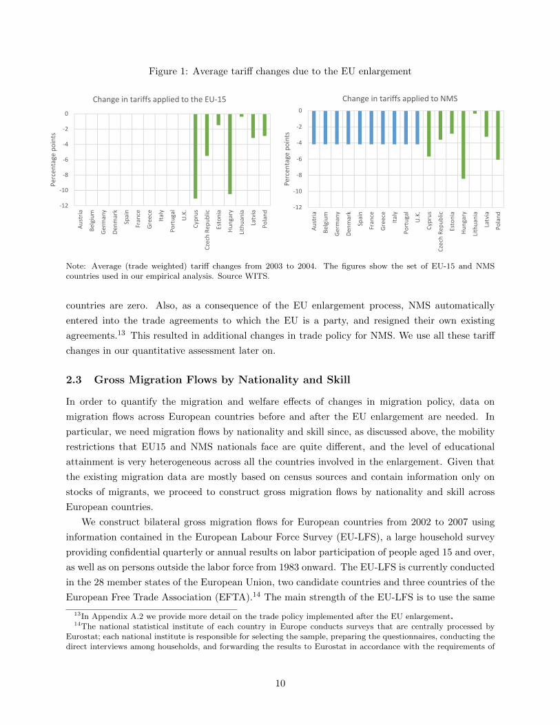
Figure 1: Average tari↵ changes due to the EU enlargement

‐12

‐10

‐8

‐6

‐4

‐2

0

Austria

Belgium

Germ

any

Denm

ark

Spain

France

Greece

Italy

Portugal

U.K.

Cyprus

Czech Re

public

Estonia

Hungary

Lithuania

Latvia

Poland

Percen

tage points

Change in tariffs applied to NMS 

‐12

‐10

‐8

‐6

‐4

‐2

0

Austria

Belgium

Germ

any

Denm

ark

Spain

France

Greece

Italy

Portugal

U.K.

Cyprus

Czech Re

public

Estonia

Hungary

Lithuania

Latvia

Poland

Percen

tage points

Change in tariffs applied to the EU‐15 

Note: Average (trade weighted) tari↵ changes from 2003 to 2004. The figures show the set of EU-15 and NMScountries used in our empirical analysis. Source WITS.

countries are zero. Also, as a consequence of the EU enlargement process, NMS automatically

entered into the trade agreements to which the EU is a party, and resigned their own existing

agreements.13 This resulted in additional changes in trade policy for NMS. We use all these tari↵

changes in our quantitative assessment later on.

2.3 Gross Migration Flows by Nationality and Skill

In order to quantify the migration and welfare e↵ects of changes in migration policy, data on

migration flows across European countries before and after the EU enlargement are needed. In

particular, we need migration flows by nationality and skill since, as discussed above, the mobility

restrictions that EU15 and NMS nationals face are quite di↵erent, and the level of educational

attainment is very heterogeneous across all the countries involved in the enlargement. Given that

the existing migration data are mostly based on census sources and contain information only on

stocks of migrants, we proceed to construct gross migration flows by nationality and skill across

European countries.

We construct bilateral gross migration flows for European countries from 2002 to 2007 using

information contained in the European Labour Force Survey (EU-LFS), a large household survey

providing confidential quarterly or annual results on labor participation of people aged 15 and over,

as well as on persons outside the labor force from 1983 onward. The EU-LFS is currently conducted

in the 28 member states of the European Union, two candidate countries and three countries of the

European Free Trade Association (EFTA).14 The main strength of the EU-LFS is to use the same

13In Appendix A.2 we provide more detail on the trade policy implemented after the EU enlargement.14The national statistical institute of each country in Europe conducts surveys that are centrally processed by

Eurostat; each national institute is responsible for selecting the sample, preparing the questionnaires, conducting thedirect interviews among households, and forwarding the results to Eurostat in accordance with the requirements of

10

concepts and definitions in every country, follow International Labour Organization guidelines using

common classifications (NACE, ISCO, ISCED, NUTS), and record the same set of characteristics in

each country. Because of these features, the EU-LFS is the basis for unemployment and education

statistics in Europe.

The survey contains information on a representative sample of the labor force in each country.

Individuals are assigned a weight to represent the share of people with the same characteristics in

the country. For each individual in a specific year, we have information on age, nationality, skills

and, crucially for our purpose, country of residence 12 months before. We use the information

on country of residence in the previous year to construct bilateral gross migration flows by year,

country of origin, nationality and skill for a group of 17 EU countries.15

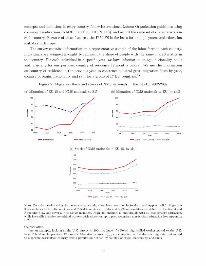
Figure 2: Migration flows and stocks of NMS nationals in the EU-15, 2002-2007

(a) Migration of EU-15 and NMS nationals to EU

50

60

70

80

90

100

Thou

sand

s

2002 2003 2004 2005 2006 2007Years

EU nationals NMS nationals

(b) Migration of NMS nationals to EU, by skill

0

20

40

60

80

100

Thousands

2002 2003 2004 2005 2006 2007Years

Overall Low-skill High-skill

(c) Stock of NMS nationals in EU-15, by skill

0

200

400

600

800

1000

1200

1400

Thousands

2002 2003 2004 2005 2006 2007Years

Overall Low-skill High-skill

Note: Own elaboration using the data set on gross migration flows described in Section 4 and Appendix B.2. Migrationflows includes 10 EU-15 countries and 7 NMS countries. EU-15 and NMS nationalities are defined in Section 4 andAppendix B.2.2 and cover all the EU-25 members. High-skill includes all individuals with at least tertiary education,while low skills include the residual workers with education up to post secondary non-tertiary education (see AppendixB.2.3).

the regulation.15As an example, looking at the U.K. survey in 2004, we know if a Polish high-skilled worker moved to the U.K.

from Poland in the previous 12 months. Migration shares, µij

n,s,t

are computed as the share of migrants that movedto a specific destination country over a population defined by country of origin, nationality and skills.

11

We group migrants in three broad nationality categories that follow immediately from the 2004

European enlargement: EU-15 nationals, NMS nationals, and Other nationals (rest of the world).

Moreover, we follow the international standard classification of education (ISCED 1997) and define

high skill labor as college educated and low skill labor as individuals with high school degree or

less. We constraint our sample to include only individuals of working age—between 15 and 65 years

old—and only countries with consistent information on nationality, skills and country of origin over

the period 2002-2007. We end up with a total of 17 countries, ten former EU members, Austria,

Belgium, Germany, Denmark, Spain, France, Greece, Italy, Portugal, and the United Kingdom,

and seven NMS, Cyprus, Czech Republic, Estonia, Hungary, Lithuania, Latvia, and Poland. Our

group of countries covers 91 percent of the 2004 EU-25 population.16

As an illustration, Figure 2 plots the gross flows and stocks of NMS migrants in EU15 countries

that arise from our constructed gross migration flows data. As we can see from the panels, the

largest fraction of migrants was low-skilled.17

2.4 Reduced-Form Evidence

With the constructed gross migration flows, we can now proceed to provide a first evidence on

the migration e↵ects of the EU enlargement by presenting reduced-form evidence on the change in

migration flows of NMS nationals to EU-15 countries after the 2004 enlargement. In particular, we

explore whether there was a significant change in migration flows after 2004, controlling by country

characteristics and time e↵ects. As an example, we use our constructed data on bilateral gross

migration flows to estimate a simple di↵erence-in-di↵erence (DD) model to evaluate the change in

the flow of NMS nationals migrating to the U.K. after 2004. We choose the U.K. since it is the

only EU-15 country in our sample that eliminated migration restrictions immediately in 2004. We

consider the NMS nationals as the treated group and the EU-15 and Other nationals as the control

group, and run the following regression,

logF i,UKn,t = �i,t + ↵NMS + �

03

I (UK, 2003) + �04

I (UK, 2004) + �05

I (UK, 2005)+

+�06

I (UK, 2006) + �07

I (UK, 2007) + "in,t,

where the dependent variable logF i,UKn,t is the (log) flow of nationality n migrants from NMS

country i to the U.K. in year t, �i,t is a set of origin-year fixed e↵ects that captures origin-time-

specific factors, and ↵NMS is a fixed e↵ect that captures possible di↵erence between NMS nationals

and the control group prior to the EU enlargement. The coe�cients {�0t}t=3�7

, interacted with

16Country surveys for Ireland, Malta, Netherlands, Sweden, Slovenia, Bulgaria, Slovakia, Luxembourg, Romaniaand Finland do not contain su�cient information to compute migration flows consistently between 2002 and 2007,so we assign these countries to the rest of the world (RoW). More information on each case is contained in AppendixB.1.

17Appendix B.2 describes in greater detail how we construct the gross migration flows, and provides a set of externalvalidation statistics.

12

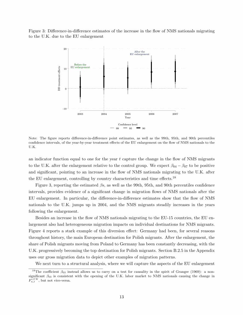
Figure 3: Di↵erence-in-di↵erence estimates of the increase in the flow of NMS nationals migratingto the U.K. due to the EU enlargement

Before theEU enlargement

After theEU enlargement

-10

0

10

20

DD

tre

atm

ent

effe

cts

2003 2004 2005 2006 2007Year

99 95 90

Confidence level

Note: The figure reports di↵erence-in-di↵erence point estimates, as well as the 99th, 95th, and 90th percentilesconfidence intervals, of the year-by-year treatment e↵ects of the EU enlargement on the flow of NMS nationals to theU.K.

an indicator function equal to one for the year t capture the change in the flow of NMS migrants

to the U.K. after the enlargement relative to the control group. We expect �04

� �07

to be positive

and significant, pointing to an increase in the flow of NMS nationals migrating to the U.K. after

the EU enlargement, controlling by country characteristics and time e↵ects.18

Figure 3, reporting the estimated �s, as well as the 99th, 95th, and 90th percentiles confidence

intervals, provides evidence of a significant change in migration flows of NMS nationals after the

EU enlargement. In particular, the di↵erence-in-di↵erence estimates show that the flow of NMS

nationals to the U.K. jumps up in 2004, and the NMS migrants steadily increases in the years

following the enlargement.

Besides an increase in the flow of NMS nationals migrating to the EU-15 countries, the EU en-

largement also had heterogeneous migration impacts on individual destinations for NMS migrants.

Figure 4 reports a stark example of this diversion e↵ect: Germany had been, for several reasons

throughout history, the main European destination for Polish migrants. After the enlargement, the

share of Polish migrants moving from Poland to Germany has been constantly decreasing, with the

U.K. progressively becoming the top destination for Polish migrants. Section B.2.5 in the Appendix

uses our gross migration data to depict other examples of migration patterns.

We next turn to a structural analysis, where we will capture the aspects of the EU enlargement

18The coe�cient �03 instead allows us to carry on a test for causality in the spirit of Granger (1969): a non-significant �03 is consistent with the opening of the U.K. labor market to NMS nationals causing the change inF

i,UK

n,t

, but not vice-versa.

13

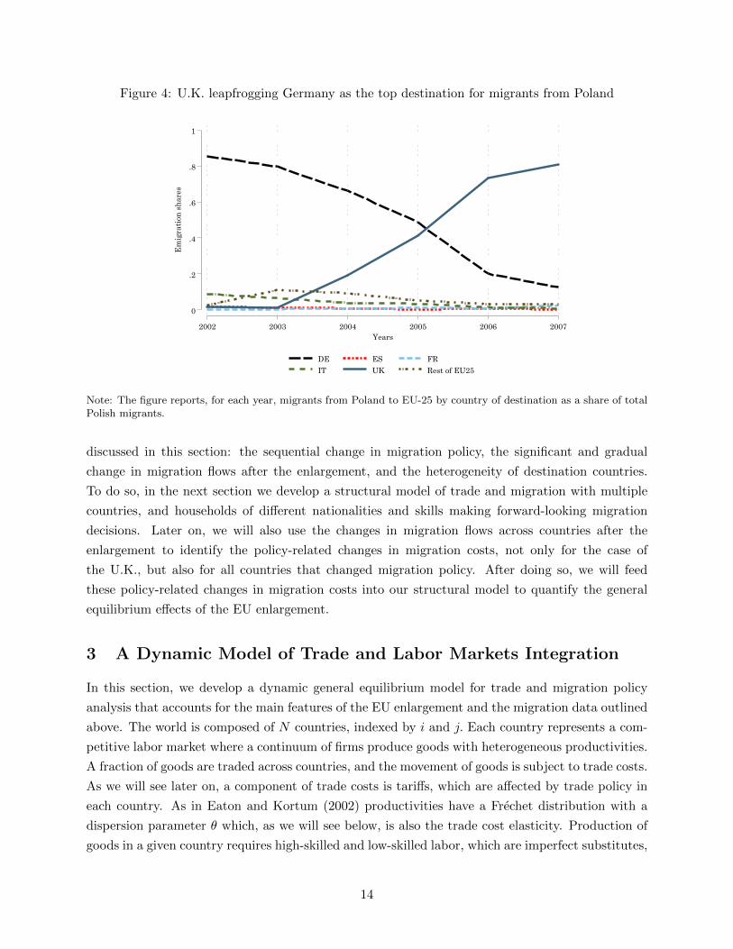
Figure 4: U.K. leapfrogging Germany as the top destination for migrants from Poland

0

.2

.4

.6

.8

1

Em

igra

tion

sh

ares

2002 2003 2004 2005 2006 2007Years

DE ES FRIT UK Rest of EU25

Note: The figure reports, for each year, migrants from Poland to EU-25 by country of destination as a share of totalPolish migrants.

discussed in this section: the sequential change in migration policy, the significant and gradual

change in migration flows after the enlargement, and the heterogeneity of destination countries.

To do so, in the next section we develop a structural model of trade and migration with multiple

countries, and households of di↵erent nationalities and skills making forward-looking migration

decisions. Later on, we will also use the changes in migration flows across countries after the

enlargement to identify the policy-related changes in migration costs, not only for the case of

the U.K., but also for all countries that changed migration policy. After doing so, we will feed

these policy-related changes in migration costs into our structural model to quantify the general

equilibrium e↵ects of the EU enlargement.

3 A Dynamic Model of Trade and Labor Markets Integration

In this section, we develop a dynamic general equilibrium model for trade and migration policy

analysis that accounts for the main features of the EU enlargement and the migration data outlined

above. The world is composed of N countries, indexed by i and j. Each country represents a com-

petitive labor market where a continuum of firms produce goods with heterogeneous productivities.

A fraction of goods are traded across countries, and the movement of goods is subject to trade costs.

As we will see later on, a component of trade costs is tari↵s, which are a↵ected by trade policy in

each country. As in Eaton and Kortum (2002) productivities have a Frechet distribution with a

dispersion parameter ✓ which, as we will see below, is also the trade cost elasticity. Production of

goods in a given country requires high-skilled and low-skilled labor, which are imperfect substitutes,

14

and fixed factors that we call structures.

In the model, time is discrete and households have perfect foresight. Households make forward-

looking labor relocation decisions subject to migration costs and idiosyncratic preferences. Each

period they decide whether to stay in the same country or to move to a di↵erent country, a decision

that depends on real wages and expected continuation values. Migration policy in each country

has an impact on migration costs, and therefore on households’ decisions.

We start by describing the problem of the households, we then set up the production structure

in each country, and finally, we derive the market clearing conditions. After doing so, we define the

equilibrium of the model.

3.1 Households

Households are forward-looking, observe the economic conditions in all countries and optimally

decide where to work. Households face costs of moving across countries and are subject to id-

iosyncratic shocks that a↵ect their moving decision. If they begin the period in a country, they

work and earn the market wage. As described above, households in a given country are of di↵erent

nationalities that we index by n, and with di↵erent skills that we index by s.

The value of a n national of skill s in country i at time t, vin,s,t, is given by

vin,s,t = log(Cis,t) + max

{j}Nj=1

{�E[vjn,s,t+1

]�mijn,s,t + ⌫✏jn,s,t},

where Cis,t is the consumption aggregator that we describe below. The term mij

n,s,t is the migration

cost from country i to country j at time t for a household native from country n and skill level s.

The migration cost, mijn,s,t in our model is time varying, as it can be impacted by changes to

migration policy. Specifically, we allow mobility costs to have a non-policy and a policy component,

that is, mijn,s,t = mij

n,s,t+mpolijn,s,t, where mijn,s,t is the non-policy component of the cost of migrating

from country i to country j for a household of nationality n and skill s, and mpolijn,s,t is the policy

component that is impacted by migration restrictions. Moreover, we allow non-policy migration to

also be time-varying and include origin-specific components, destination-specific components, and

bilateral components, that is mijn,s,t = mi

n,s,t + mjn,s,t + mij

n,s,t.

We assume that idiosyncratic preference shocks ✏jn,s,t are stochastic i.i.d. of a Type-I extreme

value distribution with zero mean, and with dispersion parameter ⌫ that later on we will relate it

to the migration cost elasticity. Finally, � is the discount factor. The presence of migration costs

and idiosyncratic preferences generates a gradual adjustment of flows in response to changes in the

economy since only the fraction of households with idiosyncratic preference for a location that more

than o↵set the migration cost will relocate each period.

Using the properties of the Type-I extreme value distribution, we can solve for the expected

(expectation over ✏) lifetime utility of a worker of nationality n and skill s in country i, namely

15

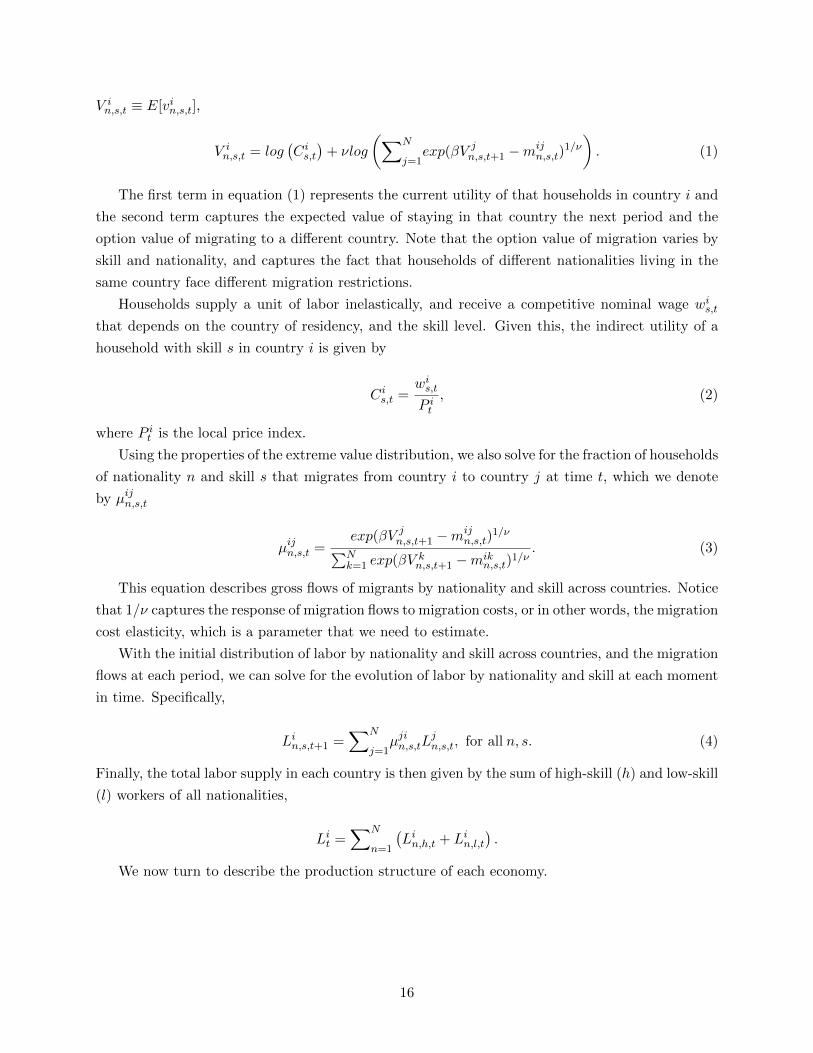
V in,s,t ⌘ E[vin,s,t],

V in,s,t = log

�

Cis,t

�

+ ⌫log

✓

XN

j=1

exp(�V jn,s,t+1

�mijn,s,t)

1/⌫

◆

. (1)

The first term in equation (1) represents the current utility of that households in country i and

the second term captures the expected value of staying in that country the next period and the

option value of migrating to a di↵erent country. Note that the option value of migration varies by

skill and nationality, and captures the fact that households of di↵erent nationalities living in the

same country face di↵erent migration restrictions.

Households supply a unit of labor inelastically, and receive a competitive nominal wage wis,t

that depends on the country of residency, and the skill level. Given this, the indirect utility of a

household with skill s in country i is given by

Cis,t =

wis,t

P it

, (2)

where P it is the local price index.

Using the properties of the extreme value distribution, we also solve for the fraction of households

of nationality n and skill s that migrates from country i to country j at time t, which we denote

by µijn,s,t

µijn,s,t =

exp(�V jn,s,t+1

�mijn,s,t)

1/⌫

PNk=1

exp(�V kn,s,t+1

�mikn,s,t)

1/⌫. (3)

This equation describes gross flows of migrants by nationality and skill across countries. Notice

that 1/⌫ captures the response of migration flows to migration costs, or in other words, the migration

cost elasticity, which is a parameter that we need to estimate.

With the initial distribution of labor by nationality and skill across countries, and the migration

flows at each period, we can solve for the evolution of labor by nationality and skill at each moment

in time. Specifically,

Lin,s,t+1

=XN

j=1

µjin,s,tL

jn,s,t, for all n, s. (4)

Finally, the total labor supply in each country is then given by the sum of high-skill (h) and low-skill

(l) workers of all nationalities,

Lit =

XN

n=1

�

Lin,h,t + Li

n,l,t

�

.

We now turn to describe the production structure of each economy.

16

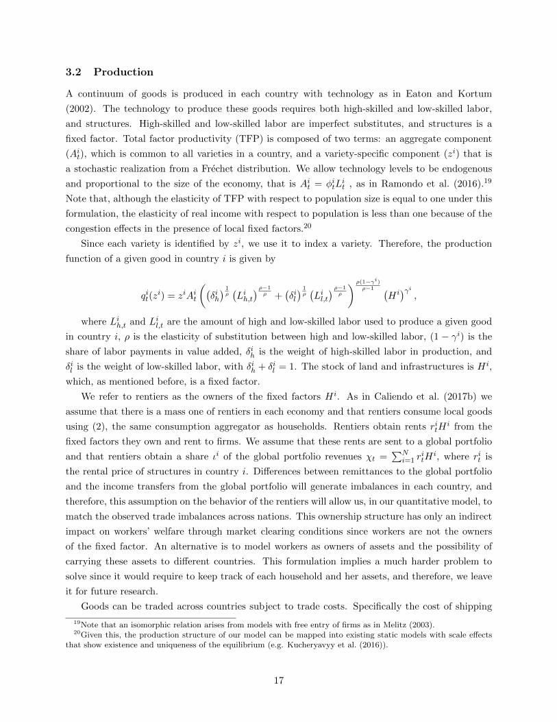
3.2 Production

A continuum of goods is produced in each country with technology as in Eaton and Kortum

(2002). The technology to produce these goods requires both high-skilled and low-skilled labor,

and structures. High-skilled and low-skilled labor are imperfect substitutes, and structures is a

fixed factor. Total factor productivity (TFP) is composed of two terms: an aggregate component

(Ait), which is common to all varieties in a country, and a variety-specific component (zi) that is

a stochastic realization from a Frechet distribution. We allow technology levels to be endogenous

and proportional to the size of the economy, that is Ait = �i

tLit , as in Ramondo et al. (2016).19

Note that, although the elasticity of TFP with respect to population size is equal to one under this

formulation, the elasticity of real income with respect to population is less than one because of the

congestion e↵ects in the presence of local fixed factors.20

Since each variety is identified by zi, we use it to index a variety. Therefore, the production

function of a given good in country i is given by

qit(zi) = ziAi

t

✓

�

�ih�

1⇢

�

Lih,t

�

⇢�1⇢ +

�

�il�

1⇢

�

Lil,t

�

⇢�1⇢

◆

⇢(1��

i)⇢�1

�

H i��i

,

where Lih,t and Li

l,t are the amount of high and low-skilled labor used to produce a given good

in country i, ⇢ is the elasticity of substitution between high and low-skilled labor, (1 � �i) is the

share of labor payments in value added, �ih is the weight of high-skilled labor in production, and

�il is the weight of low-skilled labor, with �ih + �il = 1. The stock of land and infrastructures is H i,

which, as mentioned before, is a fixed factor.

We refer to rentiers as the owners of the fixed factors H i. As in Caliendo et al. (2017b) we

assume that there is a mass one of rentiers in each economy and that rentiers consume local goods

using (2), the same consumption aggregator as households. Rentiers obtain rents ritHi from the

fixed factors they own and rent to firms. We assume that these rents are sent to a global portfolio

and that rentiers obtain a share ◆i of the global portfolio revenues �t =PN

i=1

ritHi, where rit is

the rental price of structures in country i. Di↵erences between remittances to the global portfolio

and the income transfers from the global portfolio will generate imbalances in each country, and

therefore, this assumption on the behavior of the rentiers will allow us, in our quantitative model, to

match the observed trade imbalances across nations. This ownership structure has only an indirect

impact on workers’ welfare through market clearing conditions since workers are not the owners

of the fixed factor. An alternative is to model workers as owners of assets and the possibility of

carrying these assets to di↵erent countries. This formulation implies a much harder problem to

solve since it would require to keep track of each household and her assets, and therefore, we leave

it for future research.

Goods can be traded across countries subject to trade costs. Specifically the cost of shipping

19Note that an isomorphic relation arises from models with free entry of firms as in Melitz (2003).20Given this, the production structure of our model can be mapped into existing static models with scale e↵ects

that show existence and uniqueness of the equilibrium (e.g. Kucheryavyy et al. (2016)).

17

goods from country j to country i is given by ijt = (1 + ⌧ ijt )dijt , where dijt is an iceberg-type trade

cost, which includes non-tari↵ trade barriers, and ⌧ ijt is an ad-valorem tari↵.

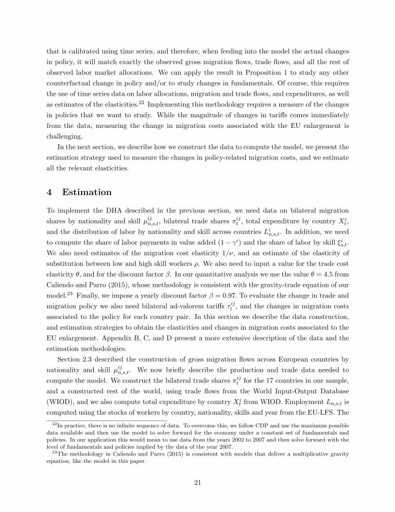
As in Eaton and Kortum (2002), using the properties of the Frechet distribution we can solve

for the bilateral trade shares ⇡ijt and the price index P i

t as a function of factor prices, productivities

and trade costs. Specifically,

⇡ijt =

Ajt (

ijt x

jt )

�✓

PNk=1

Akt (

ikt xkt )

�✓, (5)

P it =

⇣

PNj=1

Ajt (

ijt x

jt )

�✓⌘� 1

✓

, (6)

where xit is the unit price of an input bundle, namely

xit ⌘ ⇣i�

�ih(wih,t)

1�⇢ + �il(wil,t)

1�⇢�

(1��

i)1�⇢ (rit)

�i

, (7)

where ⇣i is a constant. We now describe the market clearing conditions and the equilibrium of the

model.

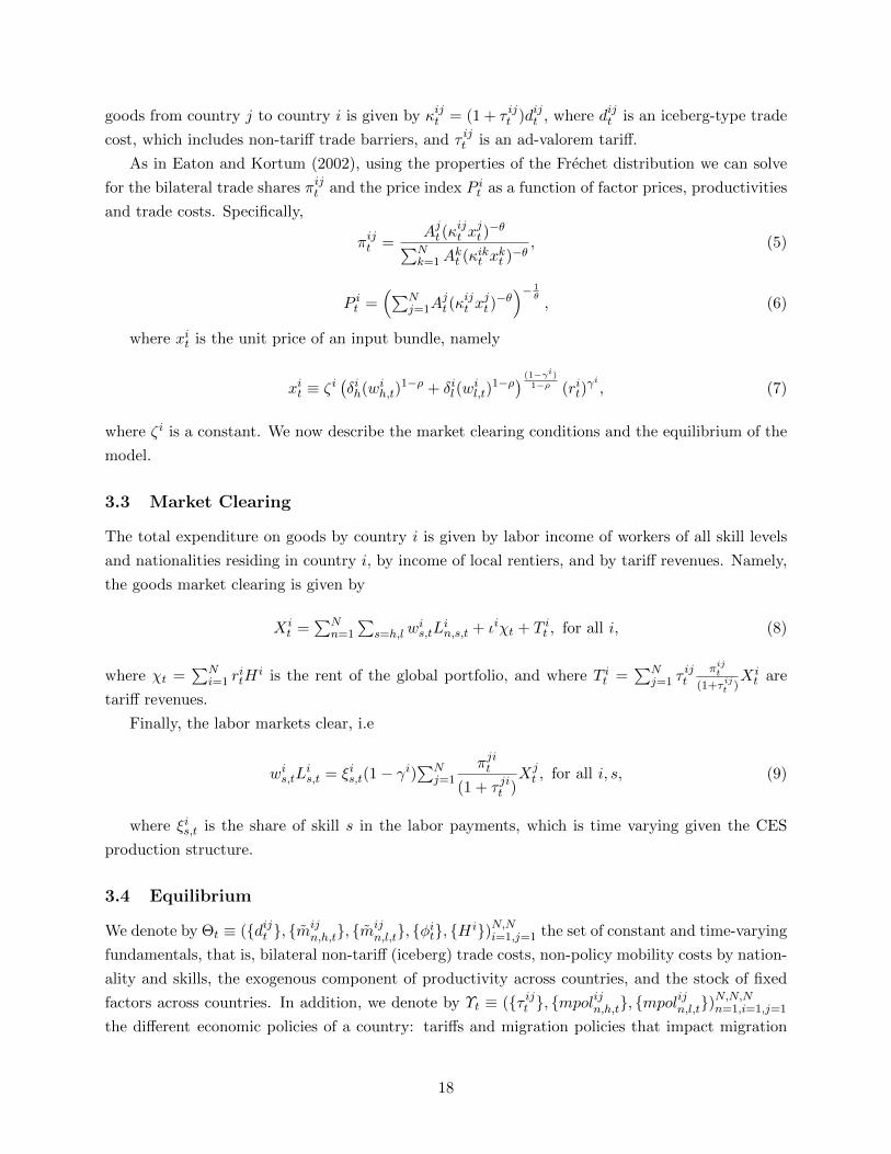
3.3 Market Clearing

The total expenditure on goods by country i is given by labor income of workers of all skill levels

and nationalities residing in country i, by income of local rentiers, and by tari↵ revenues. Namely,

the goods market clearing is given by

Xit =

PNn=1

P

s=h,l wis,tL

in,s,t + ◆i�t + T i

t , for all i, (8)

where �t =PN

i=1

ritHi is the rent of the global portfolio, and where T i

t =PN

j=1

⌧ ijt⇡ij

t

(1+⌧ ijt

)

Xit are

tari↵ revenues.

Finally, the labor markets clear, i.e

wis,tL

is,t = ⇠is,t(1� �i)

PNj=1

⇡jit

(1 + ⌧ jit )Xj

t , for all i, s, (9)

where ⇠is,t is the share of skill s in the labor payments, which is time varying given the CES

production structure.

3.4 Equilibrium

We denote by ⇥t ⌘ ({dijt }, {mijn,h,t}, {m

ijn,l,t}, {�i

t}, {H i})N,Ni=1,j=1

the set of constant and time-varying

fundamentals, that is, bilateral non-tari↵ (iceberg) trade costs, non-policy mobility costs by nation-

ality and skills, the exogenous component of productivity across countries, and the stock of fixed

factors across countries. In addition, we denote by ⌥t ⌘ ({⌧ ijt }, {mpolijn,h,t}, {mpolijn,l,t})N,N,Nn=1,i=1,j=1

the di↵erent economic policies of a country: tari↵s and migration policies that impact migration

18

costs mijn,s,t. The state of the economy is given by the distribution of labor across each market

at a given moment in time Lt =n

Lin,h,t, L

in,l,t

oN,N

n=1,i=1

. We now seek to define the equilibrium of

the model given fundamentals, trade policies, and migration policies. First, we formally define the

static equilibrium, which is given by the set of factor prices that solve the static trade equilibrium.

Definition 1. Given (Lt,⇥t,⌥t), the static equilibrium is a set {wih,t, w

il,t, r

it}Ni=1

of factor prices

that solves the static sub-problem given by the equilibrium conditions (5), (6), (7), (8), and (9).

We denote by !is,t ⌘ wi

s,t/Pit real income and by !i

s,t(Lt,⇥t,⌥t) the solution of the static

equilibrium given (Lt,⇥t,⌥t). We now define the sequential competitive equilibrium of the model

given a sequence of fundamentals and policies:

Definition 2. Given an initial allocation of labor L0

, a sequence of fundamentals {⇥t}1t=0

, and a

sequence of policies {⌥t}1t=0

, a sequential competitive equilibrium of the model is a sequence

{Ln,s,t, µn,s,t, Vn,s,t,!is,t(Lt,⇥t,⌥t)}N,1

n=1,t=0

for s = {h, l}, that solves the households’ dynamic prob-

lem, equilibrium conditions (1), (3), (4), and the temporary equilibrium at each t.

Definition 2 illustrates the equilibrium of the model given an initial condition on the state of the

economy and for a given sequence of fundamentals and policies. Our goal now is to use the model

to study the trade, migration and welfare e↵ects of changes to trade and migration policies. We do

so in the multi-country version of the model calibrated to the EU economies and a constructed rest

of the world. Taking a large scale model to the data requires estimating a large set of unknown

parameters—technologies, iceberg trade costs, the non-policy component of migration costs, and

the endowments of fixed factors—that we refer to as fundamentals. We use the method proposed

by CDP, dynamic hat algebra (henceforth DHA), to take the model to the data to study the e↵ects

of changes to trade and migration policies. The key advantage of DHA is that we can conduct our

quantitative analysis without estimating the fundamentals of the economy. We now express the

equilibrium conditions of the model in relative time di↵erences and show how we can use the model

and data to study the e↵ects of the EU enlargement.

3.5 Solving for Policy Changes

Suppose we want to study the e↵ects of changes in policy from {⌥t}1t=0

! {⌥ 0t}1t=0

. Let yt+1

⌘yt+1

/yt denote the relative time change of a variable, and let yt+1

⌘ y0t+1

/yt+1

denote the relative

time di↵erence of the variable under a sequence of policies {⌥ 0t}1t=0

relative to the sequence of

policies {⌥t}1t=0

.

For instance, if yt+1

are prices, yt+1

is the relative change in prices as a consequence of the

change in policy. Given this notation we can write the equilibrium conditions of the model for a

given change in the sequence of policies. Importantly, what the next proposition shows is that,

19

given data on the allocations of the economy, we can study the e↵ects of a change in policy without

information on the sequence of fundamentals. To simplify notation let ˆmpolij

n,s,t ⌘ exp(mpol0ijn,s,t+1

�mpol0ijn,s,t)/ exp(mpolijn,s,t+1

�mpolijn,s,t) , and uin,s,t ⌘ exp(V 0in,s,t+1

�V 0in,s,t)/ exp(V

in,s,t+1

�V in,s,t).

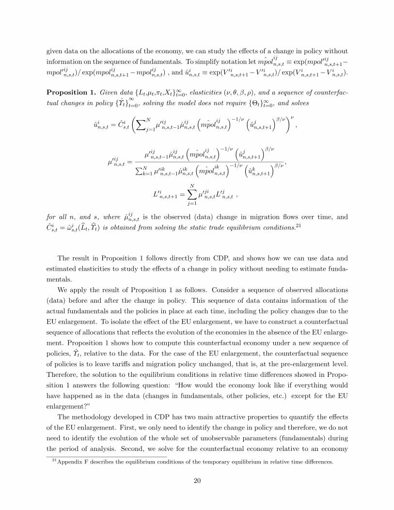
Proposition 1. Given data {Lt,µt,⇡t,Xt}1t=0

, elasticities (⌫, ✓,�, ⇢), and a sequence of counterfac-

tual changes in policy ˆ{⌥t}1t=0

, solving the model does not require {⇥t}1t=0

, and solves

uin,s,t = Cis,t

✓

XN

j=1

µ0ijn,s,t�1

µijn,s,t

⇣

ˆmpolij

n,s,t

⌘�1/⌫ ⇣

ujn,s,t+1

⌘�/⌫◆⌫

,

µ0ijn,s,t =

µ0ijn,s,t�1

µijn,s,t

⇣

ˆmpolij

n,s,t

⌘�1/⌫ ⇣

ujn,s,t+1

⌘�/⌫

PNk=1

µ0ikn,s,t�1

µikn,s,t

⇣

ˆmpolik

n,s,t

⌘�1/⌫ ⇣

ukn,s,t+1

⌘�/⌫,

L0in,s,t+1

=NX

j=1

µ0jin,s,tL

0jn,s,t ,

for all n, and s, where µijn,s,t is the observed (data) change in migration flows over time, and

Cis,t = !i

s,t(bLt, b⌥t) is obtained from solving the static trade equilibrium conditions.21

The result in Proposition 1 follows directly from CDP, and shows how we can use data and

estimated elasticities to study the e↵ects of a change in policy without needing to estimate funda-

mentals.

We apply the result of Proposition 1 as follows. Consider a sequence of observed allocations

(data) before and after the change in policy. This sequence of data contains information of the

actual fundamentals and the policies in place at each time, including the policy changes due to the

EU enlargement. To isolate the e↵ect of the EU enlargement, we have to construct a counterfactual

sequence of allocations that reflects the evolution of the economies in the absence of the EU enlarge-

ment. Proposition 1 shows how to compute this counterfactual economy under a new sequence of

policies, ⌥t, relative to the data. For the case of the EU enlargement, the counterfactual sequence

of policies is to leave tari↵s and migration policy unchanged, that is, at the pre-enlargement level.

Therefore, the solution to the equilibrium conditions in relative time di↵erences showed in Propo-

sition 1 answers the following question: “How would the economy look like if everything would

have happened as in the data (changes in fundamentals, other policies, etc.) except for the EU

enlargement?”

The methodology developed in CDP has two main attractive properties to quantify the e↵ects

of the EU enlargement. First, we only need to identify the change in policy and therefore, we do not

need to identify the evolution of the whole set of unobservable parameters (fundamentals) during

the period of analysis. Second, we solve for the counterfactual economy relative to an economy

21Appendix F describes the equilibrium conditions of the temporary equilibrium in relative time di↵erences.

20

that is calibrated using time series, and therefore, when feeding into the model the actual changes

in policy, it will match exactly the observed gross migration flows, trade flows, and all the rest of

observed labor market allocations. We can apply the result in Proposition 1 to study any other

counterfactual change in policy and/or to study changes in fundamentals. Of course, this requires

the use of time series data on labor allocations, migration and trade flows, and expenditures, as well

as estimates of the elasticities.22 Implementing this methodology requires a measure of the changes

in policies that we want to study. While the magnitude of changes in tari↵s comes immediately

from the data, measuring the change in migration costs associated with the EU enlargement is

challenging.

In the next section, we describe how we construct the data to compute the model, we present the

estimation strategy used to measure the changes in policy-related migration costs, and we estimate

all the relevant elasticities.

4 Estimation

To implement the DHA described in the previous section, we need data on bilateral migration

shares by nationality and skill µijn,s,t, bilateral trade shares ⇡ij

t , total expenditure by country Xit ,

and the distribution of labor by nationality and skill across countries Lin,s,t. In addition, we need

to compute the share of labor payments in value added (1� �i) and the share of labor by skill ⇠is,t.

We also need estimates of the migration cost elasticity 1/⌫, and an estimate of the elasticity of

substitution between low and high skill workers ⇢. We also need to input a value for the trade cost

elasticity ✓, and for the discount factor �. In our quantitative analysis we use the value ✓ = 4.5 from

Caliendo and Parro (2015), whose methodology is consistent with the gravity-trade equation of our

model.23 Finally, we impose a yearly discount factor � = 0.97. To evaluate the change in trade and

migration policy we also need bilateral ad-valorem tari↵s ⌧ ijt , and the changes in migration costs

associated to the policy for each country pair. In this section we describe the data construction,

and estimation strategies to obtain the elasticities and changes in migration costs associated to the

EU enlargement. Appendix B, C, and D present a more extensive description of the data and the

estimation methodologies.

Section 2.3 described the construction of gross migration flows across European countries by

nationality and skill µijn,s,t. We now briefly describe the production and trade data needed to

compute the model. We construct the bilateral trade shares ⇡ijt for the 17 countries in our sample,

and a constructed rest of the world, using trade flows from the World Input-Output Database

(WIOD), and we also compute total expenditure by country Xit from WIOD. Employment Ln,s,t is

computed using the stocks of workers by country, nationality, skills and year from the EU-LFS. The

22In practice, there is no infinite sequence of data. To overcome this, we follow CDP and use the maximum possibledata available and then use the model to solve forward for the economy under a constant set of fundamentals andpolicies. In our application this would mean to use data from the years 2002 to 2007 and then solve forward with thelevel of fundamentals and policies implied by the data of the year 2007.

23The methodology in Caliendo and Parro (2015) is consistent with models that deliver a multiplicative gravityequation, like the model in this paper.

21

share of labor payments in value added (1��i) is computed with information on labor compensation

retrieved from the socio economic accounts of the WIOD. The share of labor by skill ⇠is,t in total

labor payment is obtained using labor compensation data by skill from the socio economic account

of the WIOD data set.

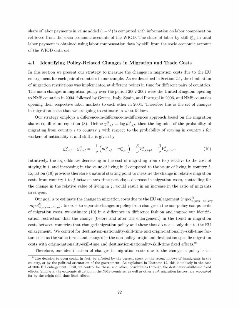
4.1 Identifying Policy-Related Changes in Migration and Trade Costs

In this section we present our strategy to measure the changes in migration costs due to the EU

enlargement for each pair of countries in our sample. As we described in Section 2.1, the elimination

of migration restrictions was implemented at di↵erent points in time for di↵erent pairs of countries.

The main changes in migration policy over the period 2002-2007 were the United Kingdom opening

to NMS countries in 2004, followed by Greece, Italy, Spain, and Portugal in 2006, and NMS countries

opening their respective labor markets to each other in 2004. Therefore this is the set of changes

in migration costs that we are going to estimate in what follows.

Our strategy employs a di↵erence-in-di↵erence-in-di↵erences approach based on the migration

shares equilibrium equation (3). Define yijn,s,t ⌘ logµijn,s,t, then the log odds of the probability of

migrating from country i to country j with respect to the probability of staying in country i for

workers of nationality n and skill s is given by

yijn,s,t � yiin,s,t = �1

⌫

⇣

mijn,s,t �mii

n,s,t

⌘

+�

⌫V jn,s,t+1

� �

⌫V in,s,t+1

. (10)

Intuitively, the log odds are decreasing in the cost of migrating from i to j relative to the cost of

staying in i, and increasing in the value of living in j compared to the value of living in country i.

Equation (10) provides therefore a natural starting point to measure the change in relative migration

costs from country i to j between two time periods; a decrease in migration costs, controlling for

the change in the relative value of living in j, would result in an increase in the ratio of migrants

to stayers.

Our goal is to estimate the change in migration costs due to the EU enlargement (mpolijn,post�enlarg.

-mpolijn,pre�enlarg). In order to separate changes in policy from changes in the non-policy components

of migration costs, we estimate (10) in a di↵erence in di↵erence fashion and impose our identifi-

cation restriction that the change (before and after the enlargement) in the trend in migration

costs between countries that changed migration policy and those that do not is only due to the EU

enlargement. We control for destination-nationality-skill-time and origin-nationality-skill-time fac-

tors such as the value terms and changes in the non-policy origin and destination specific migration

costs with origin-nationality-skill-time and destination-nationality-skill-time fixed e↵ects.24

Therefore, our identification of changes in migration costs due to the change in policy is in-

24The decision to open could, in fact, be a↵ected by the current stock or the recent inflows of immigrants in thecountry, or by the political orientation of the government. As explained in Footnote 12, this is unlikely in the caseof 2004 EU enlargement. Still, we control for these, and other, possibilities through the destination-skill-time fixede↵ects. Similarly, the economic situation in the NMS countries, as well as other push migration factors, are accountedfor by the origin-skill-time fixed e↵ects.

22

ternally consistent with both the model developed in Section 3 and our migration cost structure

discussed in the subsection 3.1. We next describe in more detail how we proceed to identify the

changes in migration costs due to the enlargement for each of the policy changes in our period of

analysis.

4.1.1 Example: U.K. Policy-Related Changes in Migration Costs Applied to NMS

To explain in more detail our identification strategy, we start by describing the estimation of the

policy-related change in the cost of migrating from NMS to the U.K. We then follow with the rest of

changes to migration policy. In the case of the U.K. we consider three sets of gross migration flows:

from NMS countries to the U.K., our treated group in the di↵erence-in-di↵erence jargon; from NMS

countries to Austria, Belgium, Denmark, France, and Germany (EU-5), our first control group, that

corresponds to a set of EU countries that did not open their labor market to NMS countries before

2008; and from EU-5 to the U.K., the second control group. Starting from equation (10) and using

our migration cost structure discussed in the subsection 3.1, we can express equation (10) as a

function of origin-specific factors, destination-specific factors, non-policy bilateral mobility costs

and the cost associated to migration policy:

yijn,s,t � yiin,s,t = �1

⌫mpolijn,s,t � 1

⌫

✓

min,s,t �

1

⌫mii

n,s,t

◆

� �

⌫V in,s,t+1

(11)

� 1

⌫mj

n,s,t +�

⌫V jn,s,t+1

� 1

⌫mij

n,s,t.

The left-hand side terms in equation (11) are the log migration flows to U.K. and control groups

minus stayers. The first term in the right-hand side of equation (11) captures the policy component

of migration costs, the second and third terms represent the origin-specific factors, the fourth and

fifth terms represent the destination-specific factors, and the last term represents the bilateral non-

policy component of migration costs. In our empirical model, we capture the origin specific factors

with origin-skill-time fixed e↵ects, and the destination specific factors with destination-skill-time

fixed e↵ects. Notice that our first control group identifies the origin fixed e↵ects, and the second

control group identifies the destination fixed e↵ects. The bilateral non-policy component will be

captured with a bilateral dummy, whose coe�cient will measure the migration cost pre-enlargement

from NMS countries to the U.K. relative to the migration costs from NMS countries to the EU-5

group and from the EU-5 group to the U.K. Finally, the change in costs due to the policy will be

captured with a bilateral and time-varying dummy, whose coe�cient will measure the change in

these relative migration costs before and after the enlargement, our object of interest. We pool the

flows of low and high-skilled workers for the bilateral dummies to capture the fact that changes in

migration policy were non-discriminatory across skills and nationalities. Therefore, our empirical

model resulting from our structural model is given by:

23

yijn,s,t � yiin,s,t = �U.K.n,s,t In,s,t (j = U.K.) +

P

o2NMS ↵on,s,tIn,s,t (i = o)+

+�U.K.n

P

o2NMS In,s,t (j = U.K., i = o)+

+�U.K.n,post

P

o2NMS In,s,t (j = U.K., i = o, t 2 post) + "ijn,s,t,

(12)

where I (.) is an indicator function, �U.K.n,s,t represents the coe�cients of a set of year-skill dummies

for when the destination is the U.K., ↵on,s,t represents the coe�cients of a set of year-skill dummies

for each source NMS country, �U.K.n is the coe�cient of a dummy for when the origin is an NMS

country and the destination is the U.K., and �U.K.n,post is the coe�cient of a dummy for when the

origin is an NMS country, the destination is the U.K., and t belongs to the post 2003 period.25

Finally, "ijn,s,t is a random disturbance of relative migration costs and it is assumed to be orthogonal

to changes in migration policy.

The coe�cient �U.K.n,post is then our main coe�cient of interest, representing the change in migra-

tion costs between the pre- and post-enlargement periods, normalized by �1/⌫, i.e.

�U.K.n,post ⌘ �1

⌫

⇣

mpolNMS,UKNMS,post�enlarg. �mpolNMS,UK

NMS,pre�enlarg.

⌘

. (13)

In other words, given an estimate of the migration elasticity, �U.K.n,post provides an estimate of the

average change in the cost of migrating from NMS countries to the U.K. due to the enlargement

process, after controlling for any destination-skill-nationality-time and origin-skill-nationality-time

confounding factors.26

Note the importance of using three sets of gross flows, from NMS to the U.K., from NMS to

EU-5 countries, and from EU-5 countries to the U.K., in order to identify destination-nationality-

skill-time and origin-nationality-skill-time fixed e↵ects.27 The coe�cient �U.K.n,post is then the sum of

three components: the average change in the cost of migrating from NMS countries to the U.K., our

target, minus both the change in the cost of migrating from NMS countries to EU-5 countries and

the change in the cost of migrating from EU-5 countries to the U.K. for NMS nationals. We exploit

the fact that (i) EU-5 countries did not open their labor markets to NMS countries in the sample

period (which justifies choosing EU-5 as the control group), and (ii) those NMS nationals residing

in EU-5 before the EU enlargement did not experience changes in migration costs associated to

the EU enlargement.28 Appendix C.1 and C.2 provide support for the common trend assumption

25Note that the origin-nationality-skill-time fixed e↵ects ↵

o

n,s,t

also control for changes in the cost of staying incountry o for a s-skilled n national.

26Note that one could have estimated a coe�cient across NMS origin countries and skills. Instead, we constrainedthe point estimate to be equal across skill groups. This does not mean that the migration costs are the same fordi↵erent skill groups, it only means that the change in policy was proportionally equal across di↵erent skill groups.

27Given that we are aggregating data at the origin-destination-year level for a given nationality we account forpossible random e↵ects common to all individuals migrating from the same origin country to the same destinationcountry in the same year.

28One reason why this is the case is that NMS nationals already legally working in one of the old member states atthe date of accession for an uninterrupted period of at least 12 months continue to have access to the labor market

24

Table 1: Estimates of Changes in Migration Costs, NMS nationals

NMS nationals

Destination j ! U.K. (2004) GR (2006) IT (2006) ES (2006) PT (2006)

�j

n,post

3.52∗∗∗

(1.11)

2.29∗∗

(0.83)

1.01∗

(0.55)

0.18

(0.54)

1.01∗∗∗

(0.49)

R2 0.96 0.97 0.98 0.97 0.98

Obs. 564 564 564 564 564

Notes: The table reports di↵erence-in-di↵erence estimates, from separate regressions, of the change in migrationcost from NMS countries to either the United Kingdom (U.K.), Greece (GR), Italy (IT), Spain (ES), or Portugal(PT) for NMS nationals. Recall, from equation (13), that a positive estimate implies a reduction in migration costs.The treatment period (post) is 2004-2007 for the U.K., and 2006-2007 for the other destinations. Parenthesesincludes robust standard errors, ⇤⇤⇤ p<0.01, ⇤⇤ p<0.05, ⇤ p<0.10. Similar significance is obtained if instead we usetwo-way clustering at the origin-destination-country level.

underlying the di↵erence-in-di↵erence strategy.

4.1.2 EU Countries Policy-Related Change in Migration Costs Applied to NMS

The top panel of table 1 presents our estimates of the policy-related changes in migration costs

for the case of NMS nationals moving from NMS countries to the U.K, Greece, Italy, Spain, and

Portugal. As we can see, all estimates are positive and significant (except for Spain), pointing to

a reduction in the cost of migrating from NMS to Europe for NMS nationals both in 2004 and

2006.29 These coe�cients are hard to interpret since they reflect the change in the migration cost

scaled by the migration elasticity and measured in units of utility. To understand the magnitude,

in terms of consumption, real wages, etc., of these changes we need to use these estimates as inputs

in our quantitative model.

4.1.3 Placebo Experiments

To support our identification strategy we also run placebo experiments. The intuition is that we

expect the costs of migrating from NMS countries to the U.K., Greece, Italy, Spain, and Portugal

not to have changed for EU-15 nationals as a consequence of the EU enlargement. The bottom

panel of table 2 reports these estimates, and reassuringly shows no change in the migration costs

due to the enlargement from NMS to Europe for those that already were European citizens.

of that member state. NMS nationals who had in 2004 legally worked in e.g. Germany for at least 12 months couldkeep working there even if the German labor market was not generally open to NMS nationals.

29Recall, from equation (13), that a positive estimate implies a reduction in migration costs.

25

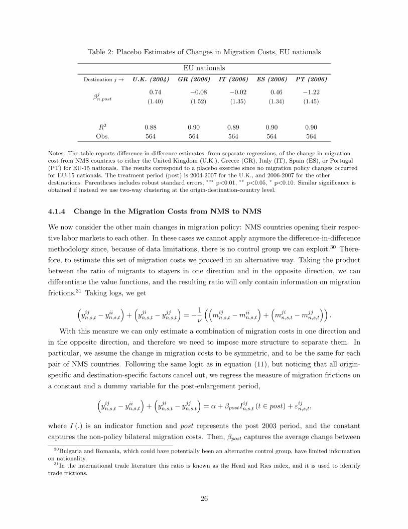
Table 2: Placebo Estimates of Changes in Migration Costs, EU nationals

EU nationals

Destination j ! U.K. (2004) GR (2006) IT (2006) ES (2006) PT (2006)

�j

n,post

0.74

(1.40)

�0.08

(1.52)

�0.02

(1.35)

0.46

(1.34)

�1.22

(1.45)

R2 0.88 0.90 0.89 0.90 0.90

Obs. 564 564 564 564 564

Notes: The table reports di↵erence-in-di↵erence estimates, from separate regressions, of the change in migrationcost from NMS countries to either the United Kingdom (U.K.), Greece (GR), Italy (IT), Spain (ES), or Portugal(PT) for EU-15 nationals. The results correspond to a placebo exercise since no migration policy changes occurredfor EU-15 nationals. The treatment period (post) is 2004-2007 for the U.K., and 2006-2007 for the otherdestinations. Parentheses includes robust standard errors, ⇤⇤⇤ p<0.01, ⇤⇤ p<0.05, ⇤ p<0.10. Similar significance isobtained if instead we use two-way clustering at the origin-destination-country level.

4.1.4 Change in the Migration Costs from NMS to NMS

We now consider the other main changes in migration policy: NMS countries opening their respec-

tive labor markets to each other. In these cases we cannot apply anymore the di↵erence-in-di↵erence

methodology since, because of data limitations, there is no control group we can exploit.30 There-

fore, to estimate this set of migration costs we proceed in an alternative way. Taking the product

between the ratio of migrants to stayers in one direction and in the opposite direction, we can

di↵erentiate the value functions, and the resulting ratio will only contain information on migration

frictions.31 Taking logs, we get

⇣

yijn,s,t � yiin,s,t

⌘

+⇣

yjin,s,t � yjjn,s,t

⌘

= �1

⌫

⇣⇣

mijn,s,t �mii

n,s,t

⌘

+⇣

mjin,s,t �mjj

n,s,t

⌘⌘

.

With this measure we can only estimate a combination of migration costs in one direction and

in the opposite direction, and therefore we need to impose more structure to separate them. In

particular, we assume the change in migration costs to be symmetric, and to be the same for each

pair of NMS countries. Following the same logic as in equation (11), but noticing that all origin-

specific and destination-specific factors cancel out, we regress the measure of migration frictions on

a constant and a dummy variable for the post-enlargement period,

⇣

yijn,s,t � yiin,s,t

⌘

+⇣

yjin,s,t � yjjn,s,t

⌘

= ↵+ �postIijn,s,t (t 2 post) + "ijn,s,t,

where I (.) is an indicator function and post represents the post 2003 period, and the constant

captures the non-policy bilateral migration costs. Then, �post captures the average change between

30Bulgaria and Romania, which could have potentially been an alternative control group, have limited informationon nationality.

31In the international trade literature this ratio is known as the Head and Ries index, and it is used to identifytrade frictions.

26

Table 3: Changes in Migration Costs, NMS to NMS

NMS nationals

�post 1.71⇤⇤⇤

(0.49)

R2 0.99Obs. 252Notes: ⇤⇤⇤

p < 0.01, robust standard errors

the pre- and post-enlargement period of the migration frictions, which measures the policy-related

change in migration costs.32

Table 3 reports the results, and shows a reduction in the cost of migrating from NMS to NMS

countries, for NMS nationals, in 2004.

4.1.5 Change in Trade Policy

Finally, we employ bilateral tari↵s ⌧ ijt between each pair of countries and the rest of the world, using

information from the World Integrated Trade Solution (WITS) data set, to capture changes in trade

costs due to the EU enlargement. We use e↵ectively applied rates and we combine information

from two di↵erent data sets, the TRAINS data set and the WTO data set, to have complete and

consistent information on tari↵s over time.33

Armed with this set of estimates of the changes in trade and migration costs associated with

the EU enlargement , we now proceed to estimate the necessary elasticities for our quantitative

analysis.

4.2 International Migration Elasticity

The migration elasticity is needed to evaluate the welfare e↵ects associated to changes in the barriers

to migrate; welfare e↵ects depend on the magnitude of the change in barriers, and on how sensitive

the decision to migrate is to the barriers themselves. Artuc et al. (2010) and CDP, provide estimates

of the elasticities for internal migration flows, while here we deal with international migration. We

therefore adapt the methodology of Artuc and McLaren (2015) to the structure of our model,

and apply it to the flows of EU nationals within the EU, to provide a value for the international

migration elasticity.34

The first stage of the methodology is a fixed-e↵ect estimation that uses the migration share

equation (3) and bilateral gross migration flows data to estimate value di↵erences and the migration

cost function normalized by ⌫. The second stage of the methodology relies on the Bellman equation.

32We also used the same strategy in order to identify the changes in costs of migrating to NMS for EU nationals.For this case we used the flows of EU nationals from the EU to NMS before and after the change in policy. Given thatthere where not many flows over our sample period and no significant variation in the flows we ended up obtainingnot economically significant estimates for this case.

33In Appendix B.3.1 we explain in detail how we construct the bilateral tari↵ data for each country pair.34We describe in detail the implementation of the methodology and report the results, both for the baseline case

and for the extension with public good described later, in Appendix D.

27

We insert the estimated value di↵erences from the first stage into the Bellman equation, and

construct a linear regression to retrieve the international migration elasticity by exploiting the

variation in real wages. We estimate the second stage model as an IV regression, using two-period

lagged values of real wages as instruments, and clustering standard errors at the country level.35

In our preferred specification with � = 0.97 we obtain an elasticity of 0.44—significant at 1

percent—which implies a value of ⌫ of 2.3. This is the value that we use when performing our

quantitative analysis.

4.3 Elasticity of Substitution Between Low- and High-Skilled Workers

In this section, we provide the estimate of the elasticity of substitution between low and high-

skilled workers that will be used to quantify the e↵ects of the EU enlargement.36 Following the

literature, low-skilled workers include workers with a high-school degree or less, and high-skilled

workers are workers with some college education and college graduates. We estimate the elasticity

of substitution using detailed information on workers’ wages and hours, as well as firms’ location

and industry, from the Portuguese matched employer-employee data (Quadros de Pessoal) for the

period 1991-2008.37 Our estimation strategy builds on standard approaches (e.g. Katz and Murphy

(1992)), but we instrument the endogeneity of the relative supply of high to low-skilled workers.

We estimate the following econometric model based on the equilibrium conditions of the theory

laid out in Section 3,

lnwvrh,t

wvrl,t

= �1

⇢ln

Lvrh,t

Lvrl,t

+ ↵vr + "vrt , (14)

where⇣

wvrh,t/w

vrl,t

⌘

is the ratio of high- and low-skilled workers’ wages in industry v and region r (in

Portugal),⇣

Lvrh,t/L

vrl,t

⌘

is the corresponding relative supply, and ⇢ is the elasticity of substitution

between low and high-skilled workers. Finally, we have written the relative weight of high- and

low-skilled workers (1/⇢) ln (�vrh /�vrl ) as the sum of an industry-region fixed e↵ect and a residual

industry-region-time e↵ect ↵vr + "vrt .

The main di�culty faced by researchers in this area is that the relative number of more educated

35We emphasize three merits of the Artuc and McLaren (2015) methodology: First, the estimation strategy doesnot require taking logarithm of probabilities. Given that most of the migration shares are very small this is animportant feature that avoids causing large errors and imprecise estimates, and allows us to work with 17 countries.Second, we can be agnostic about exactly what information workers have when they form their expectations of futurewages, and only assume that forecast errors are mean zero conditional on contemporaneous information. Third,we impose only a mild assumption on bilateral migration costs: we assume that migration costs for EU nationalsflowing across EU-15 member states did not vary over time and skills. Note, however, that we can still let the costof migrating out of country i, and into country j, be skill-dependent.

36We will also check the robustness of our results using estimates of the elasticity obtained via alternative econo-metric approaches, as well as estimates from the literature.

37We resort to Quadros de Pessoal for a number of reasons. First, Quadros de Pessoal’s provides an exhaustivecoverage of firms and their workers over a long time-span. Currently, the data set collects information on about350,000 firms and 3 million employees per year. Second, we can estimate an elasticity of substitution between lowand high-skill workers that is consistent with the skills definitions from the EU-LFS. Third, we can estimate anelasticity of substitution using data from an European country, and we can compare our findings to other estimatesavailable in the literature for other countries. Last but not least, we can exploit the richness of the data to implementan instrumental variable strategy, described below, that facilitates the identification of the elasticity of substitution.

28

workers and their relative wages are determined simultaneously by demand and supply. Because

of that, the relative supply term⇣

Lvrh,t/L

vrl,t

⌘

in equation (14) could be correlated with industry-

region demand shocks ("vrt ), making it di�cult to identify the elasticity of substitution via OLS.

We tackle this issue by using instrumental variable estimation.38 Our instrument for⇣

Lvrh,t/L

vrl,t

⌘

is constructed using information on the local availability of low- and high-skilled workers that

change firm because of displacement, and in particular because of firm closure.39 A firm closure

can be considered as an exogenous shock to a worker’s career, since it results in a separation of all

plant’s workers and it is not related to the worker’s own job performance (Dustmann and Meghir

(2005)). Moreover, when instrumenting the relative labor supply of a given industry, we consider

only closures of firms that belong to other industries, so that their closure is hardly related to the

market of the industry under consideration. Finally, as workers tend to search and accept more

easily new jobs in the same local labor market of the past job, we consider closures of firms that

belong to the same region of the industry under consideration. Overall, the local availability of

displaced workers can then be considered as an exogenous labor supply shock for local firms. Figure

5 shows the correlation between the instrumented variable and the instrument.

Figure 5: Relative supply of high-skilled workers and displaced high-skilled workers, by industryand region, 1992-2005

-5

-4

-3

-2

-1

Log

rela

tive

supp

ly o

f ski

lled

wor

kers

-6 -5 -4 -3 -2 -1Log relative supply of displaced high-skill workers of other industries in the same region

Note: Own elaboration using the matched employer-employee data set Quadros de Pessoal described in Section B.5and Appendix E. Low-skill includes all workers with a high-school degree or less, and high-skilled are workers withsome college education and college graduates. Each circle in the plot corresponds to an industry-region-year, whereregions are approximately NUTS II (5 regions), and industries are NACE 1-digit. The dashed line corresponds tothe predicted values of a linear OLS model, with slope of 0.53 (with standard error 0.050) and R

2 equal to 0.39.

38Many papers estimating the elasticity of substitution between low- and high-skilled workers do not considerendogeneity issues. Two important exceptions are Angrist (1995) and Ciccone and Peri (2005). Angrist (1995)estimate the relationship between the return to schooling and the supply of more educated workers among Palestiniansin the West Bank and the Gaza Strip during the 1980s, exploiting the fact that the increase in the supply of moreeducated workers was mainly driven by the creation of new local institutions of higher education. Ciccone and Peri(2005) estimate the long-run elasticity of substitution between low- and high-skilled workers at the U.S. state levelusing data from five 1950-1990 decennial censuses. They exploit time- and state-specific child labor and compulsoryschool attendance laws as instruments.

39Displacement is usually defined as the permanent and involuntary separation of workers from their jobs withoutcause (i.e. for economic reasons). Displacement occurs when a firm shuts down or substantially downsizes.

29

Employing the methodology and data outlined above (and described more in detail in Appendix

E), we obtain an elasticity of 4, which is the number we use in our quantitative analysis. The

estimate of the elasticity of substitution is pretty robust to alternative di↵erent specifications,

methodologies, and levels of data aggregation (Appendix E). Our estimate is slightly above those

commonly found for the U.S. (Katz and Murphy (1992); Johnson (1997); Krusell et al. (2000);

Ottaviano and Peri (2012); Ciccone and Peri (2005)) which ranges between 1.5 and 2.5, but below

the elasticity of substitution of 5 between low- and medium-skilled workers found for Germany

(Dustmann et al. (2009)). Since the set of European countries we consider in the quantitative

analysis is pretty diverse in terms of labor market institutions and workforce characteristics we

consider our benchmark estimate of 4 as a good compromise.

5 Economic E↵ects of the 2004 EU Enlargement

In this section, we use the estimated policy-related changes in migration costs, and the observed

changes in tari↵s, to quantify the migration and welfare e↵ects of the EU enlargement. We first

compute the migration e↵ects from the actual changes to migration and trade policies over the

period 2002-2007, and we then quantify the welfare e↵ects. We also use our model to study the

interaction between trade openness and migration policy, and to decompose the role of the di↵erent

mechanisms of the model in shaping the welfare e↵ects.

5.1 Migration E↵ects

We start by quantifying the migration e↵ects from the EU enlargement. In particular, with our

structural model we want to answer questions such as: How did the stock of new member states

(NMS) migrants in EU-15 countries respond to the EU enlargement? Was NMS migration gradual

or a once for all process? What was the change in the stock of NMS migrants in EU-15 countries

across skill groups, and in the short and long run? What would have been the migration e↵ects in

the absence of changes to trade policy?

To compute the migration e↵ects, we feed into our structural model the estimated changes

in migration costs and the observed changes in tari↵s over 2002-2007, and compute the change

migration e↵ects compared with an economy where migration and trade policies stayed unchanged.

Figure 6 displays the evolution of the stock of NMS nationals in EU-15 countries (for all workers and

by skill). The darker line shows the evolution of the stock in the baseline economy with the actual

changes to migration and trade policy between 2002-2007. The dashed line shows the evolution

of the stock of NMS nationals in the counterfactual economy, where we hold migration costs and

tari↵s constant at the levels before the EU enlargement. Therefore, the di↵erence between the two

lines is the migration e↵ects from the EU enlargement. From the figure, panel a, we can see that

the increase in the stock of NMS migrants in EU-15 countries is realized very gradually over time.

For instance, three years after the EU enlargement (that is, in 2007) the stock of NMS nationals in

EU-15 countries increases by 0.03 percentage points, while ten years after the implementation, the

30

Figure 6: Evolution of the stock of NMS migrants in EU15 countries (percent)

Notes: This figure presents the stock of NMS migrants in EU-15 countries. The green lines show the evolution ofthis stock with actual changes to trade and migration policies. The dashed lines show the evolution holding tradeand migration policies unchanged. The panel, (left column) presents the results for all workers, and panel b (rightcolumn) presents the results for high and low-skilled workers.

stock raises by 0.23 percentage points. We find that in steady state, the stock of NMS nationals in

EU-15 countries increases by 0.63 percentage points, or by about 3.3 million, which corresponds to

about 5 percent of the population of the NMS countries in 2004. Across individual countries, we

find that the United Kingdom is the country that experienced the largest increase in the stock of

NMS nationals.

We now turn to compute the change in the stock of migrants across di↵erent skills, and after

doing so, we discuss the interaction between migration and trade policies. Figure 6, panel b,

presents the evolution of the stock of low and high skill NMS migrants in EU15 countries. In Table

4, columns (1) and (3), we also decompose the stock of NMS nationals in EU-15 countries by skill.

We find that the EU enlargement primarily increases the migration of low-skilled NMS workers to

EU-15 countries, and to a much lesser extent the migration of high-skilled workers. For instance,

as we can see from the table, the stock of NMS high-skilled workers in EU-15 countries increases by

0.014 percentage points, or 51.9 thousands by 2007, by 0.06 percentage points or 215.8 thousands

by 2015, and by 0.13 percentage points or by about 485.2 thousands in the long run. We find that

the change in the stock of NMS low-skilled workers is much larger. Specifically, for the case of

low-skilled workers, the stock of NMS nationals in EU-15 countries increases by 0.066 percentage

points or 246.1 thousands by 2007, by 0.3 percentage points or 1.1 million by 2015, and by 0.75

percentage points or by about 2.8 million in the steady state.

We can also use the model to compute what the migration e↵ects would have been in the

absence of changes to trade policy. In columns (2) and (4) of Table 4, we compute the change

in the stock of NMS nationals in EU-15 countries holding trade policy constant. We find that

migration would have been larger in the absence of changes to trade policy. For instance, the stock

of low-skilled workers would have been about 150 thousands larger in the long run, and the stock of

31

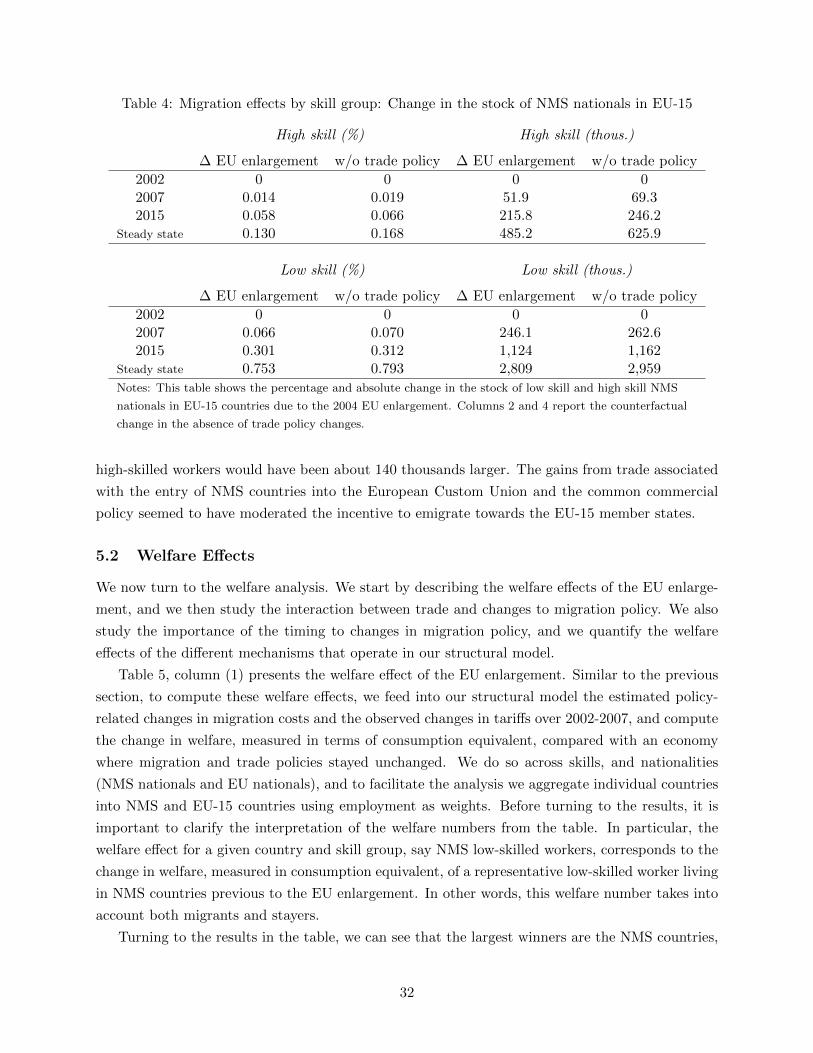
Table 4: Migration e↵ects by skill group: Change in the stock of NMS nationals in EU-15

High skill (%) High skill (thous.)

� EU enlargement w/o trade policy � EU enlargement w/o trade policy2002 0 0 0 02007 0.014 0.019 51.9 69.32015 0.058 0.066 215.8 246.2

Steady state 0.130 0.168 485.2 625.9

Low skill (%) Low skill (thous.)

� EU enlargement w/o trade policy � EU enlargement w/o trade policy2002 0 0 0 02007 0.066 0.070 246.1 262.62015 0.301 0.312 1,124 1,162

Steady state 0.753 0.793 2,809 2,959Notes: This table shows the percentage and absolute change in the stock of low skill and high skill NMS

nationals in EU-15 countries due to the 2004 EU enlargement. Columns 2 and 4 report the counterfactual

change in the absence of trade policy changes.

high-skilled workers would have been about 140 thousands larger. The gains from trade associated

with the entry of NMS countries into the European Custom Union and the common commercial

policy seemed to have moderated the incentive to emigrate towards the EU-15 member states.

5.2 Welfare E↵ects

We now turn to the welfare analysis. We start by describing the welfare e↵ects of the EU enlarge-

ment, and we then study the interaction between trade and changes to migration policy. We also

study the importance of the timing to changes in migration policy, and we quantify the welfare

e↵ects of the di↵erent mechanisms that operate in our structural model.

Table 5, column (1) presents the welfare e↵ect of the EU enlargement. Similar to the previous

section, to compute these welfare e↵ects, we feed into our structural model the estimated policy-

related changes in migration costs and the observed changes in tari↵s over 2002-2007, and compute

the change in welfare, measured in terms of consumption equivalent, compared with an economy

where migration and trade policies stayed unchanged. We do so across skills, and nationalities

(NMS nationals and EU nationals), and to facilitate the analysis we aggregate individual countries

into NMS and EU-15 countries using employment as weights. Before turning to the results, it is

important to clarify the interpretation of the welfare numbers from the table. In particular, the

welfare e↵ect for a given country and skill group, say NMS low-skilled workers, corresponds to the

change in welfare, measured in consumption equivalent, of a representative low-skilled worker living

in NMS countries previous to the EU enlargement. In other words, this welfare number takes into

account both migrants and stayers.

Turning to the results in the table, we can see that the largest winners are the NMS countries,

32

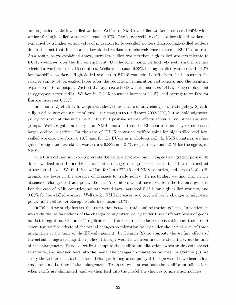
and in particular the low-skilled workers. Welfare of NMS low-skilled workers increases 1.46%, while

welfare for high-skilled workers increases 0.97%. The larger welfare e↵ect for low-skilled workers is

explained by a higher option value of migration for low-skilled workers than for high-skilled workers

due to the fact that, for instance, low-skilled workers are relatively more scarce in EU-15 countries.

As a result, as we explained above, more low-skilled workers than high-skilled workers migrate to

EU-15 countries after the EU enlargement. On the other hand, we find relatively smaller welfare

e↵ects for workers in EU-15 countries. Welfare increases 0.23% for high-skilled workers and 0.12%

for low-skilled workers. High-skilled workers in EU-15 countries benefit from the increase in the

relative supply of low-skilled labor after the reduction in migration restrictions, and the resulting

expansion in total output. We find that aggregate NMS welfare increases 1.41%, using employment

to aggregate across skills. Welfare in EU-15 countries increases 0.14%, and aggregate welfare for

Europe increases 0.36%.

In column (2) of Table 5, we present the welfare e↵ects of only changes to trade policy. Specifi-

cally, we feed into our structural model the changes to tari↵s over 2002-2007, but we hold migration

policy constant at the initial level. We find positive welfare e↵ects across all countries and skill

groups. Welfare gains are larger for NMS countries than for EU countries as they experience a

larger decline in tari↵s. For the case of EU-15 countries, welfare gains for high-skilled and low-

skilled workers, are about 0.18%, and for the EU-15 as a whole as well. In NMS countries, welfare

gains for high and low-skilled workers are 0.83% and 81%, respectively, and 0.81% for the aggregate

NMS.

The third column in Table 5 presents the welfare e↵ects of only changes to migration policy. To

do so, we feed into the model the estimated changes in migration costs, but hold tari↵s constant

at the initial level. We find that welfare for both EU-15 and NMS countries, and across both skill

groups, are lower in the absence of changes to trade policy. In particular, we find that in the

absence of changes to trade policy the EU-15 countries would have lost from the EU enlargement.

For the case of NMS countries, welfare would have increased 0.13% for high-skilled workers, and

0.63% for low-skilled workers. Welfare for NMS increases by 0.57% with only changes to migration

policy, and welfare for Europe would have been 0.07%.

In Table 6 we study further the interaction between trade and migration policies. In particular,

we study the welfare e↵ects of the changes to migration policy under three di↵erent levels of goods

market integration. Column (1) replicates the third column in the previous table, and therefore it

shows the welfare e↵ects of the actual changes to migration policy under the actual level of trade

integration at the time of the EU-enlargement. In Column (2) we compute the welfare e↵ects of

the actual changes to migration policy if Europe would have been under trade autarky at the time

of the enlargement. To do so, we first compute the equilibrium allocations when trade costs are set

to infinite, and we then feed into the model the changes to migration policies. In Column (3), we

study the welfare e↵ects of the actual changes to migration policy if Europe would have been a free

trade area at the time of the enlargement. To do so, we first compute the equilibrium allocations

when tari↵s are eliminated, and we then feed into the model the changes to migration policies.

33

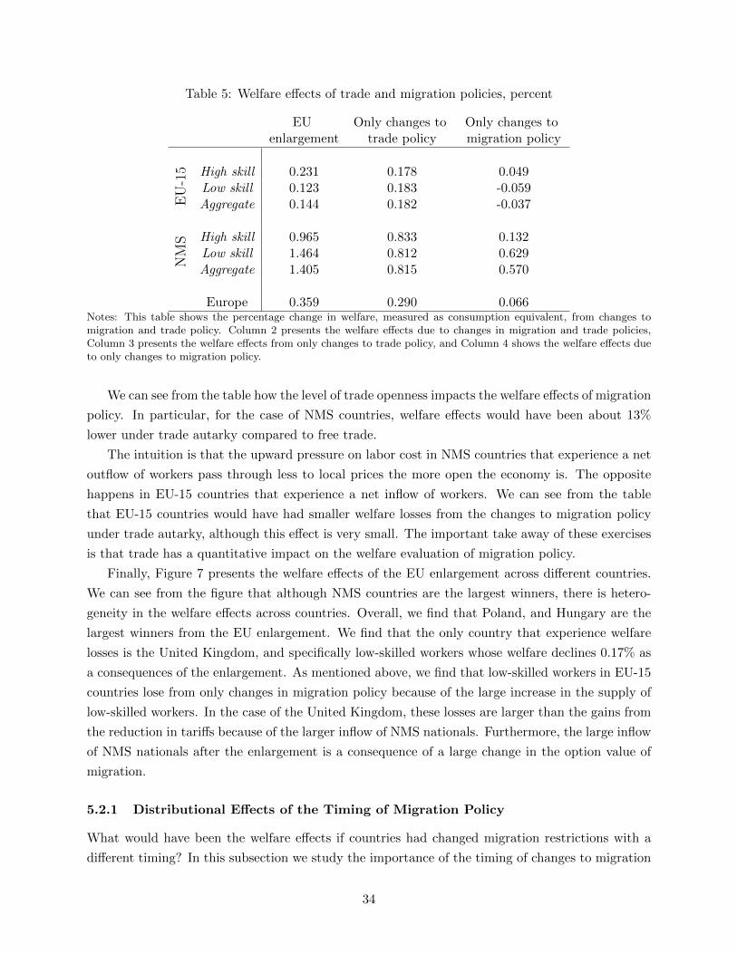
Table 5: Welfare e↵ects of trade and migration policies, percent

EU Only changes to Only changes toenlargement trade policy migration policy

EU-15 High skill 0.231 0.178 0.049

Low skill 0.123 0.183 -0.059Aggregate 0.144 0.182 -0.037

NMS High skill 0.965 0.833 0.132

Low skill 1.464 0.812 0.629Aggregate 1.405 0.815 0.570

Europe 0.359 0.290 0.066Notes: This table shows the percentage change in welfare, measured as consumption equivalent, from changes tomigration and trade policy. Column 2 presents the welfare e↵ects due to changes in migration and trade policies,Column 3 presents the welfare e↵ects from only changes to trade policy, and Column 4 shows the welfare e↵ects dueto only changes to migration policy.

We can see from the table how the level of trade openness impacts the welfare e↵ects of migration

policy. In particular, for the case of NMS countries, welfare e↵ects would have been about 13%

lower under trade autarky compared to free trade.

The intuition is that the upward pressure on labor cost in NMS countries that experience a net

outflow of workers pass through less to local prices the more open the economy is. The opposite

happens in EU-15 countries that experience a net inflow of workers. We can see from the table

that EU-15 countries would have had smaller welfare losses from the changes to migration policy

under trade autarky, although this e↵ect is very small. The important take away of these exercises

is that trade has a quantitative impact on the welfare evaluation of migration policy.

Finally, Figure 7 presents the welfare e↵ects of the EU enlargement across di↵erent countries.

We can see from the figure that although NMS countries are the largest winners, there is hetero-

geneity in the welfare e↵ects across countries. Overall, we find that Poland, and Hungary are the

largest winners from the EU enlargement. We find that the only country that experience welfare

losses is the United Kingdom, and specifically low-skilled workers whose welfare declines 0.17% as

a consequences of the enlargement. As mentioned above, we find that low-skilled workers in EU-15

countries lose from only changes in migration policy because of the large increase in the supply of

low-skilled workers. In the case of the United Kingdom, these losses are larger than the gains from

the reduction in tari↵s because of the larger inflow of NMS nationals. Furthermore, the large inflow

of NMS nationals after the enlargement is a consequence of a large change in the option value of

migration.

5.2.1 Distributional E↵ects of the Timing of Migration Policy

What would have been the welfare e↵ects if countries had changed migration restrictions with a

di↵erent timing? In this subsection we study the importance of the timing of changes to migration

34

Table 6: Trade openness and welfare e↵ects of migration policy (percent)

Only changes to Changes to migration policy Changes to migration policymigration policy under trade autarky under free trade

EU-15 High skill 0.049 0.061 0.048

Low skill -0.059 -0.052 -0.060Aggregate -0.037 -0.030 -0.039

NMS High skill 0.132 0.078 0.141

Low skill 0.629 0.572 0.638Aggregate 0.570 0.514 0.580

Europe 0.066 0.063 0.067Notes: This table shows the percentage change in welfare, measured as consumption equivalent, due to the actualchanges to migration policy. Column 2 presents the welfare e↵ects under the actual level of trade openness, Column3 shows the welfare e↵ects under trade autarky, and Column 4 shows the welfare e↵ects under free trade.

policy. To do so, Figure 8 panel a, shows the welfare e↵ects for EU-15 and NMS countries, relative

to the actual e↵ects, assuming that instead of changing policy as they did over 2002-2007, countries

would have changed policy in di↵erent years. That is, we study the e↵ects from a bilateral reduction

in migration restrictions between the United Kingdom, Greece, Italy, Spain, Portugal, and NMS

all happening in the year 2004, or 2005, and so on. The figure shows that delaying the opening in

migration, NMS countries would have lower welfare gains compared to the actual gains, and the

same is true for the case of EU-15 high-skilled workers. For instance, if all countries had changed

migration policy in 2012, welfare gains for NMS low-skilled workers would have been about 8% lower

than the actual gains. On the other hand, we find that low-skilled workers in EU-15 countries would

have been better of by delaying changes to migration policy. The result is explained by the fact that

EU-15 low-skilled workers gained from changes to trade policy but lost from changes to migration

policy, and therefore, delaying the changes to migration policy increases the relative impact of trade

policy in their welfare.

In part, the previous result is driven by the United Kingdom that is the only country that

experiences welfare losses for low-skilled workers. Given that, on panel b we investigate the welfare

e↵ects on the United Kingdom of delaying the change in migration policy. The figure plots the

welfare e↵ects under di↵erent opening years, and we find that both welfare losses of low-skilled

workers and welfare gains of high-skilled workers would have been smaller by delaying opening to

migration.

5.2.2 Accounting for the Provision of Public Goods

In this section we extend our model to account for additional congestion e↵ects coming from the

provision of public goods. In particular, this extension is motivated by evidence on the fact that

migrants are net beneficiaries of the welfare system across countries, and therefore are more likely

35

Figure 7: Welfare e↵ects, percent

(a) High skill

AUT

BEL

CYP

CZE

DEU

DNK

EST

ESP

FRA

GRC

HUN

ITA

LTU

LVA

POL

PRT

GBR

(b) Low skill

AUT

BEL

CYP

CZE

DEU

DNK

EST

ESP

FRA

GRC

HUN

ITA

LTU

LVA

POL

PRT

GBR

(c) Aggregate

AUT

BEL

CYP

CZE

DEU

DNK

EST

ESP

FRA

GRC

HUN

ITA

LTU

LVA

POL

PRT

GBR

AUT

BEL

CYP

CZE

DEU

DNK

EST

ESP

FRA

GRC

HUN

ITA

LTU

LVA

POL

PRT

GBR

(1.5,2.5](.9,1.5](.7,.9](.5,.7](.3,.5](0,.3][-.5,0]

% change

Notes: These figures present the welfare e↵ects of the EU enlargement across di↵erent countries and skill groups.

to use social benefits and consume public goods than natives.40 To capture the congestion of public

goods due to immigration, we assume that households derive some utility from the per capita

provision of public goods in the economy. Specifically, the indirect utility of a household with skill

s in country i is given by

Cis,t =

✓

Gi

Lit

◆↵i

(1� ⌧ iL)wis,t

P it

!

1�↵i

, (15)

where P i

t is the local price index, and ↵i is the fraction of public goods in total consumption.41

The supply of public goods, Gi, is fixed over time. In order to supply Gi the government purchases

final goods and finances its spending from three sources: tari↵ revenues, labor taxes (⌧ iL), and lump

sum transfers from the owners of fixed factors in each country. As a result, the government budget

40See Kerr and Kerr (2011) for a survey.41Similar specifications for preferences of public goods have been used recently in other quantitative studies, see

Fajgelbaum et al. (2015).

36

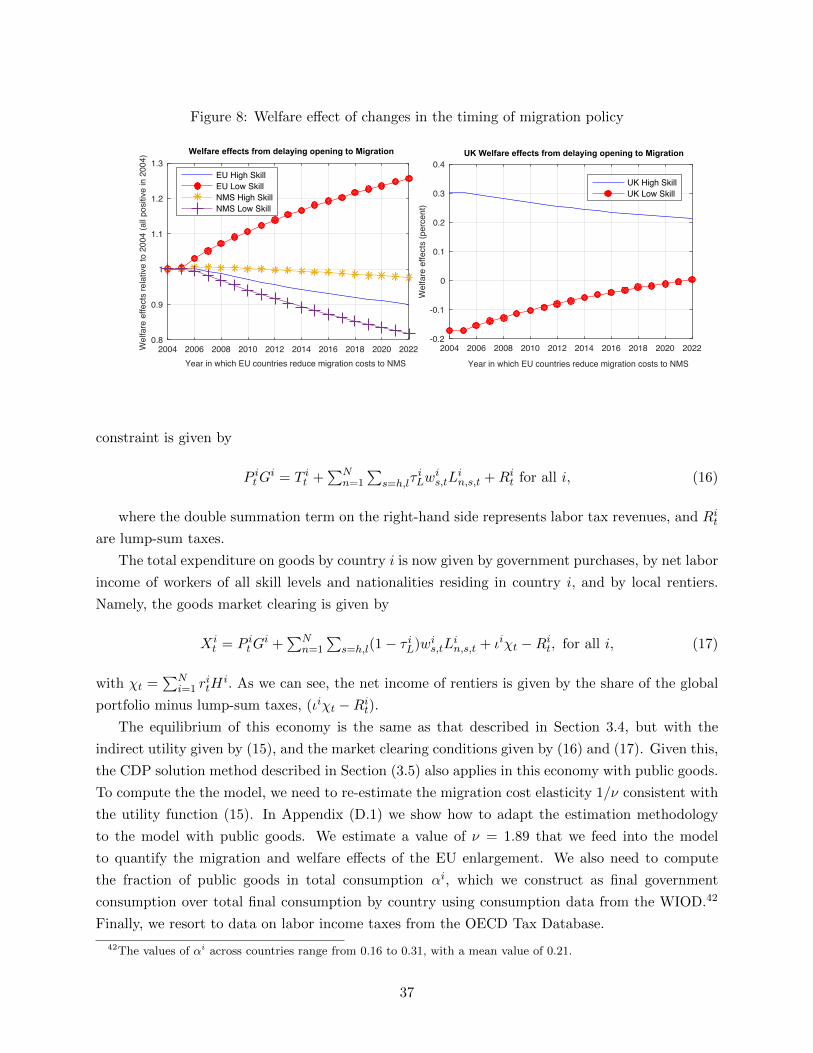
Figure 8: Welfare e↵ect of changes in the timing of migration policy

2004 2006 2008 2010 2012 2014 2016 2018 2020 2022Year in which EU countries reduce migration costs to NMS

0.8

0.9

1

1.1

1.2

1.3

Wel

fare

effe

cts

rela

tive

to 2

004

(all

posi

tive

in 2

004)

Welfare effects from delaying opening to Migration

EU High SkillEU Low SkillNMS High SkillNMS Low Skill

2004 2006 2008 2010 2012 2014 2016 2018 2020 2022

Year in which EU countries reduce migration costs to NMS

-0.2

-0.1

0

0.1

0.2

0.3

0.4

Wel

fare

effe

cts

(per

cent

)

UK Welfare effects from delaying opening to Migration

UK High SkillUK Low Skill

constraint is given by

P itG

i = T it +

PNn=1

P

s=h,l⌧iLw

is,tL

in,s,t +Ri

t for all i, (16)

where the double summation term on the right-hand side represents labor tax revenues, and Rit

are lump-sum taxes.

The total expenditure on goods by country i is now given by government purchases, by net labor

income of workers of all skill levels and nationalities residing in country i, and by local rentiers.

Namely, the goods market clearing is given by

Xit = P i

tGi +PN

n=1

P

s=h,l(1� ⌧ iL)wis,tL

in,s,t + ◆i�t �Ri

t, for all i, (17)

with �t =PN

i=1

ritHi. As we can see, the net income of rentiers is given by the share of the global

portfolio minus lump-sum taxes, (◆i�t �Rit).

The equilibrium of this economy is the same as that described in Section 3.4, but with the

indirect utility given by (15), and the market clearing conditions given by (16) and (17). Given this,

the CDP solution method described in Section (3.5) also applies in this economy with public goods.

To compute the the model, we need to re-estimate the migration cost elasticity 1/⌫ consistent with

the utility function (15). In Appendix (D.1) we show how to adapt the estimation methodology

to the model with public goods. We estimate a value of ⌫ = 1.89 that we feed into the model

to quantify the migration and welfare e↵ects of the EU enlargement. We also need to compute

the fraction of public goods in total consumption ↵i, which we construct as final government

consumption over total final consumption by country using consumption data from the WIOD.42

Finally, we resort to data on labor income taxes from the OECD Tax Database.

42The values of ↵i across countries range from 0.16 to 0.31, with a mean value of 0.21.

37

We now turn to quantify the migration and welfare e↵ects of the EU enlargement in the model

with public goods. Starting with the migration e↵ects, we still find a very gradual increase in

the stock of NMS nationals in EU-15 country as a consequence of the enlargement. In terms

of the magnitudes, we find somewhat lower migration e↵ects in the model with public goods.

Specifically, three years after the EU enlargement (that is, in 2007) the stock of NMS nationals

in EU countries increases by 0.02 percentage points, while ten years after the implementation,

the stock raises by 0.22 percentage points. In steady state, the stock of NMS nationals in EU-15

countries increases by 0.52 percentage points as a result of the EU enlargement. In the presence of

public goods, immigration strains public goods which introduces an additional source of congestion.

As a consequence, the households’ utility and incentives to migrate reduce compared to the economy

without public goods. Across skills, we find that most of the migration, as a consequence of the

enlargement, is low-skilled, similarly to our finding in Section 5.1. In the long run, the stock of

NMS high-skilled workers in EU-15 countries increases by 0.10 percentage points or by about 361.8

thousands, while the stock of NMS low-skilled workers increases by 0.63 percentage points or by

about 2.3 million.

We now turn to the analysis of the welfare e↵ects of the EU enlargement in the presence of public

goods. Overall, in the presence of public goods we find larger welfare gains for NMS countries, and

smaller welfare gains for EU-15 countries, compared with the results in Section 5.1. This result is

explained by the fact that EU-15 countries experience a net inflow of workers, which congests public

goods and has a negative impact on welfare compared with a model without public goods. On the

other hand, the net outflow of workers in NMS countries contributes to decongesting public goods,

which has a positive e↵ect on welfare. We still find that the largest winners are the NMS countries,

and in particular the low-skilled workers. Welfare of NMS low-skilled workers increases 1.52%,

while welfare for high-skilled workers increases 1.07%. On the other hand, we find smaller welfare

e↵ects for workers in EU countries. Welfare increases 0.09% for high-skilled workers and 0.03%

for low-skilled workers. We find that aggregate NMS welfare increases 1.47%, while EU-15 welfare

increases 0.05%. Aggregate welfare for Europe increases 0.29% as a result of the EU enlargement

in the model with public goods.

Finally, Figure 9 presents the welfare e↵ects from the EU enlargement in the presence of public

goods. Poland and Hungary are the largest winners in this case, and the United Kingdom experi-

ences welfare losses. Welfare losses for low-skilled workers in the U.K. are 0.43%, and high-skilled

workers are now slightly worse o↵.

5.2.3 The Role of Scale E↵ects, Fixed Factors, and Trade Openness

In this section, we study the role of other mechanisms in shaping the welfare e↵ects of the EU

enlargement, namely, scale e↵ects, fixed factors, and trade openness. Table 7 shows the results.

Column (1) of the table reproduces the benchmark results, that is, the welfare e↵ects from changes

to migration and trade policies described in Section 5.1 and 5.2. In column (2), we shut down the

scale e↵ects (that is, we set the agglomeration elasticity equal to zero) in the benchmark model,

38

Figure 9: Welfare e↵ects with public goods, percent

(a) High skill

AUT

BEL

CYP

CZE

DEU

DNK

EST

ESP

FRA

GRC

HUN

ITA

LTU

LVA

POL

PRT

GBR

(b) Low skill

AUT

BEL

CYP

CZE

DEU

DNK

EST

ESP

FRA

GRC

HUN

ITA

LTU

LVA

POL

PRT

GBR

(c) Aggregate

AUT

BEL

CYP

CZE

DEU

DNK

EST

ESP

FRA

GRC

HUN

ITA

LTU

LVA

POL

PRT

GBR

AUT

BEL

CYP

CZE

DEU

DNK

EST

ESP

FRA

GRC

HUN

ITA

LTU

LVA

POL

PRT

GBR

(1.5,2.5](.9,1.5](.7,.9](.5,.7](.3,.5](0,.3][-.5,0]

% change

Notes: These figures present the welfare e↵ects of the EU enlargement across di↵erent countries and skill

groups with the presence of public goods.

but we let the other mechanisms operate. In this case, we still find that EU-15 and NMS countries

gain from the enlargement, but welfare gains are a bit lower in EU-15 countries and larger in NMS

countries compared with the model in which all mechanisms operate. In particular, the absence of

scale e↵ects subtracts 0.06 percentage points of welfare in EU-15 countries and adds 0.3 percentage

points of welfare in NMS countries. The reason is that the net inflow of migrants in EU-15 results

in an increase in productivity in the presence of scale e↵ects, and the NMS that have a net outflow

of workers experience a productivity decline in the presence of scale e↵ects.

Finally, in column (3) we compute the welfare e↵ects under autarky, and where we also shut

down all congestion e↵ects (infrastructure and public goods) as well as scale e↵ects. To do so, we

first compute the equilibrium allocations when trade costs are set to infinite, and we then feed into

the model the changes to migration and trade policies. Compared with the third column in Table 6

welfare is substantially di↵erent in a model without trade, scale and congestion e↵ects; welfare losses

for EU-15 are more than twice larger, and welfare gains for NMS countries are reduced by 30%.

With this final counterfactual exercise we want to emphasize again the importance of accounting

39

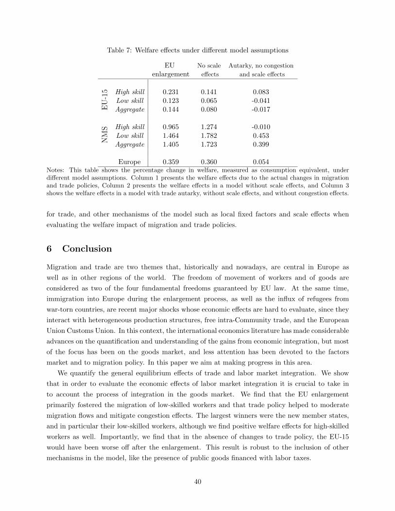
Table 7: Welfare e↵ects under di↵erent model assumptions

EU No scale Autarky, no congestion

enlargement e↵ects and scale e↵ects

EU-15 High skill 0.231 0.141 0.083

Low skill 0.123 0.065 -0.041Aggregate 0.144 0.080 -0.017

NMS High skill 0.965 1.274 -0.010

Low skill 1.464 1.782 0.453Aggregate 1.405 1.723 0.399

Europe 0.359 0.360 0.054Notes: This table shows the percentage change in welfare, measured as consumption equivalent, underdi↵erent model assumptions. Column 1 presents the welfare e↵ects due to the actual changes in migrationand trade policies, Column 2 presents the welfare e↵ects in a model without scale e↵ects, and Column 3shows the welfare e↵ects in a model with trade autarky, without scale e↵ects, and without congestion e↵ects.

for trade, and other mechanisms of the model such as local fixed factors and scale e↵ects when

evaluating the welfare impact of migration and trade policies.

6 Conclusion

Migration and trade are two themes that, historically and nowadays, are central in Europe as

well as in other regions of the world. The freedom of movement of workers and of goods are

considered as two of the four fundamental freedoms guaranteed by EU law. At the same time,

immigration into Europe during the enlargement process, as well as the influx of refugees from

war-torn countries, are recent major shocks whose economic e↵ects are hard to evaluate, since they

interact with heterogeneous production structures, free intra-Community trade, and the European

Union Customs Union. In this context, the international economics literature has made considerable

advances on the quantification and understanding of the gains from economic integration, but most

of the focus has been on the goods market, and less attention has been devoted to the factors

market and to migration policy. In this paper we aim at making progress in this area.

We quantify the general equilibrium e↵ects of trade and labor market integration. We show

that in order to evaluate the economic e↵ects of labor market integration it is crucial to take in

to account the process of integration in the goods market. We find that the EU enlargement

primarily fostered the migration of low-skilled workers and that trade policy helped to moderate

migration flows and mitigate congestion e↵ects. The largest winners were the new member states,

and in particular their low-skilled workers, although we find positive welfare e↵ects for high-skilled

workers as well. Importantly, we find that in the absence of changes to trade policy, the EU-15

would have been worse o↵ after the enlargement. This result is robust to the inclusion of other

mechanisms in the model, like the presence of public goods financed with labor taxes.

40

Our paper incorporates di↵erent but complementary elements in the analysis. We use reduced-

form analysis that exploits migration policy changes to identify changes in migration costs and key

elasticities. We build a rich dynamic general equilibrium model that includes important mechanisms

considered in the literature to quantify the migration and welfare e↵ects of actual changes to trade

and migration policies. Among other things, we show quantitatively how the e↵ects of labor market

integration are a↵ected by the extent to which countries are open to trade. Future work might aim

at studying the distributional e↵ects across sectors of the economy. Sectoral linkages are important

for trade policy quantitative analysis and they might well be also for migration policy evaluation.

References

Ahlfeldt, G. M., S. J. Redding, D. M. Sturm, and N. Wolf (2015): “The economics of

density: Evidence from the Berlin Wall,” Econometrica, 83, 2127–2189.

Allen, T. and C. Arkolakis (2014): “Trade and the Topography of the Spatial Economy,” The

Quarterly Journal of Economics, 129, 1085–1140.

Angrist, J. D. (1995): “The Economic Returns to Schooling in the West Bank and Gaza Strip,”

The American Economic Review, 85, 1065–1087.

Artuc, E., S. Chaudhuri, and J. McLaren (2010): “Trade Shocks and Labor Adjustment: A

Structural Empirical Approach,” The American Economic Review, 100, 1008–1045.

Artuc, E. and J. McLaren (2015): “Trade Policy and Wage inequality: A Structural Analysis

with Occupational and Sectoral Mobility,” Journal of International Economics, 97, 278–294.

Autor, D. H., L. F. Katz, and M. S. Kearney (2008): “Trends in US Wage Inequality:

Revising the Revisionists,” The Review of Economics and Statistics, 90, 300–323.

Baldwin, R. (1995): “The Eastern enlargement of the European Union,” European Economic

Review, 39, 474–481.

Baldwin, R., J. Francois, and R. Portes (1997): “The costs and benefits of eastern enlarge-

ment: the impact on the EU and central Europe,” Economic Policy, 12, 125–176.

Borjas, G. (1987): “Self-Selection and the Earnings of Immigrants,” NBER Working Papers 2248,

National Bureau of Economic Research, Inc.

Borjas, G. J., J. Grogger, and G. H. Hanson (2012): “Comment: On estimating elasticities

of substition,” Journal of the European Economic Association, 10, 198–210.

Bryan, G. and M. Morten (2017): “The Aggregate Productivity E↵ects of Internal Migration:

Evidence from Indonesia,” .

41

Burstein, A., G. Hanson, L. Tian, and J. Vogel (2017): “Tradability and the Labor-Market

Impact of Immigration: Theory and Evidence from the U.S.” Working Paper 23330, National

Bureau of Economic Research.

Caliendo, L., M. Dvorkin, and F. Parro (2017a): “Trade and Labor Market Dynamics:

General Equilibrium Analysis of the China Trade Shock,” mimeo, Yale University.

Caliendo, L. and F. Parro (2015): “Estimates of the Trade and Welfare E↵ects of NAFTA,”

The Review of Economic Studies, 82, 1–44.

Caliendo, L., F. Parro, E. Rossi-Hansberg, and P. Sarte (2017b): “The Impact of Regional

and Sectoral Productivity Changes on the U.S. Economy,” mimeo, Yale University.

Carneiro, A. J. M. and P. Portugal (2006): “Earnings Losses of Displaced Workers: Evidence

from a Matched Employer-Employee Dataset,” IZA DP No. 2289.

Ciccone, A. and G. Peri (2005): “Long-Run Substitutability Between More and Less Educated

Workers: Evidence from US States, 1950–1990,” The Review of Economics and Statistics, 87,

652–663.

Cosar, A. K. (2013): “Adjusting to trade liberalization: Reallocation and labor market policies,”

University of Chicago Booth School of Business, unpublished manuscript.

Cosar, A. K., N. Guner, and J. Tybout (2016): “Firm dynamics, job turnover, and wage

distributions in an open economy,” The American Economic Review, 106, 625–663.

Costinot, A. and A. Rodriguez-Clare (2014): “Trade Theory with Numbers: Quantifying

the Consequences of Globalization,” Handbook of International Economics, 197–261.

Council of the European Union (2012): “Consolidated Versions of the Treaty on European

Union and the Treaty on the Functioning of the European Union,” O�cial Journal of the Euro-

pean Union, 55.

Davis, D. R. and D. E. Weinstein (2002): “Technological Superiority and the Losses from

Migration,” NBER Working Papers 8971, National Bureau of Economic Research.

Desmet, K., D. K. Nagy, and E. Rossi-Hansberg (2016): “The Geography of Development,”

In Press, Journal of Political Economy.

Desmet, K. and E. Rossi-Hansberg (2014): “Spatial development,” The American Economic

Review, 104, 1211–1243.

di Giovanni, J., A. A. Levchenko, and F. Ortega (2015): “A Global View of Cross-Border

Migration,” Journal of the European Economic Association, 13, 168–202.

Diamond, R. (2016): “The Determinants and Welfare Implications of US Workers’ Diverging

Location Choices by Skill: 1980-2000,” American Economic Review, 106, 479–524.

42

Dix-Carneiro, R. (2014): “Trade liberalization and labor market dynamics,” Econometrica, 82,

825–885.

Dix Carneiro, R. and B. K. Kovak (2017): “Trade liberalization and regional dynamics,”

American Economic Review, forthcoming.

Dustmann, C. and T. Frattini (2011): “Immigration: the European experience,” .

Dustmann, C., T. Frattini, and A. Rosso (2015): “The E↵ect of Emigration from Poland on

Polish Wages,” The Scandinavian Journal of Economics, 117, 522–564.

Dustmann, C., J. Ludsteck, and U. Schonberg (2009): “Revisiting the German Wage Struc-

ture,” The Quarterly Journal of Economics, 124, 843–881.

Dustmann, C. and C. Meghir (2005): “Wages, Experience and Seniority,” The Review of

Economic Studies, 72, 77–108.

Eaton, J. and S. Kortum (2001): “Technology, Trade, and Growth: A Unified Framework,”

European Economic Review, 45, 742–755.

——— (2002): “Technology, Geography, and Trade,” Econometrica, 70, 1741–1779.

European Union (2003): “Documents Concerning the Accession of the Czech Republic, the

Republic of Estonia, the Republic of Cyprus, the Republic of Latvia, the Republic of Lithuania,

the Republic of Hungary, the Republic of Malta, the Republic of Poland, the Republic of Slovenia

and the Slovak Republic to the European Union,” O�cial Journal of the European Union, 46.

Fajgelbaum, P. D., E. Morales, J. C. S. Serrato, and O. M. Zidar (2015): “State

taxes and spatial misallocation,” NBER Working Papers 21760, National Bureau of Economic

Research.

Feenstra, R. C., R. Inklaar, and M. P. Timmer (2015): “The Next Generation of the Penn

World Table,” The American Economic Review, 105, 3150–3182.

Galle, S., A. Rodriguez-Clare, and M. Yi (2017): “Slicing the pie: Quantifying the aggregate

and distributional e↵ects of trade,” Unpublished manuscript, Univ. Calif., Berkeley.

Handley, K. and N. Limao (2015): “Trade and Investment Under Policy Uncertainty: Theory

and Firm Evidence,” American Economic Journal: Economic Policy, 7, 189–222.

Hanson, G. H. and M. J. Slaughter (2002): “Labor-market adjustment in open economies:

Evidence from US states,” Journal of international Economics, 57, 3–29.

——— (2016): “High-Skilled Immigration and the Rise of STEM Occupations in U.S. Employ-

ment,” Working Paper 22623, National Bureau of Economic Research.

43

Hong, G. and J. Mclaren (2016): “Are Immigrants a Shot in the Arm for the Local Economy?”

mimeo, University of Virginia.

Hummels, D., P. Minor, M. Reisman, and E. Endean (2007): “Calculating Tari↵ Equivalents

for Time in Trade,” USAID Report, March.

Hummels, D. L. and G. Schaur (2013): “Time as a Trade Barrier,” The American Economic

Review, 103, 2935–2959.

Johnson, G. E. (1997): “Changes in Earnings Inequality: the Role of Demand Shifts,” The

Journal of Economic Perspectives, 11, 41–54.

Jones, C. (1995): “R&D-Based Models of Economic Growth,” Journal of Political Economy, 103,

759–84.

Katz, L. F. and K. M. Murphy (1992): “Changes in Relative Wages, 1963–1987: Supply and

Demand Factors,” The Quarterly Journal of Economics, 107, 35–78.

Kennan, J. (2017): “Open Borders in the European Union and Beyond: Migration Flows and

Labor Market Implications,” Working Paper 23048, National Bureau of Economic Research.

Kerr, P. S. and W. R. Kerr (2011): “Economic Impacts of Immigration: A Survey,” Finnish

Economic Papers, 24, 1–32.

Klein, P. and G. Ventura (2009): “Productivity di↵erences and the dynamic e↵ects of labor

movements,” Journal of Monetary Economics, 56, 1059–1073.

Kondo, I. (2013): “Trade reforms, foreign competition, and labor market adjustments in the US,”

mimeo, Federal Reserve Board.

Kortum, S. S. (1997): “Research, Patenting, and Technological Change,” Econometrica: Journal

of the Econometric Society, 1389–1419.

Krugman, P. (1980): “Scale economies, product di↵erentiation, and the pattern of trade,” The

American Economic Review, 70, 950–959.

Krusell, P., L. E. Ohanian, J.-V. Rıos-Rull, and G. L. Violante (2000): “Capital-Skill

Complementarity and Inequality: A Macroeconomic Analysis,” Econometrica, 68, 1029–1053.

Kucheryavyy, K., G. Lyn, and A. Rodrıguez-Clare (2016): “Grounded by Gravity: A Well-

Behaved Trade Model with Industry-Level Economies of Scale,” NBER Working Papers 22484,

National Bureau of Economic Research.

Lagakos, D. and M. E. Waugh (2013): “Selection, Agriculture, and Cross-Country Productivity

Di↵erences,” American Economic Review, 103, 948–80.

44

Martincus, C. V., J. Carballo, and A. Graziano (2015): “Customs,” Journal of Interna-

tional Economics, 96, 119–137.

McLaren, J. (2017): “Globalization and Labor Market Dynamics,” Annual Review of Economics,

9, 177–200.

McLaren, J. and S. Hakobyan (2015): “Looking for local labor market e↵ects of NAFTA,”

mimeo, University of Virginia.

Melitz, M. J. (2003): “The Impact of Trade on Intra-Industry Reallocations and Aggregate

Industry Productivity,” Econometrica, 71, 1695–1725.

Menezes-Filho, N. A. and M.-A. Muendler (2011): “Labor Reallocation in Response to Trade

Reform,” Working Paper 17372, National Bureau of Economic Research.

Monte, F., S. J. Redding, and E. Rossi-Hansberg (2015): “Commuting, Migration and Local

Employment Elasticities,” Working Paper 21706, National Bureau of Economic Research.

OECD (2016): “Taxing Wages 2016,” .

Ossa, R. (2014): “Trade wars and trade talks with data,” The American Economic Review, 104,

4104–4146.

Ottaviano, G. I. and G. Peri (2012): “Rethinking the E↵ect of Immigration on Wages,” Journal

of the European Economic Association, 10, 152–197.

Ottaviano, G. I. P., G. Peri, and G. C. Wright (2013): “Immigration, O↵shoring, and

American Jobs,” American Economic Review, 103, 1925–59.

Ramondo, N., A. Rodrıguez-Clare, and M. Saborıo-Rodrıguez (2016): “Trade, Domestic

Frictions, and Scale E↵ects,” The American Economic Review, 106, 3159–3184.

Redding, S. J. (2016): “Goods trade, factor mobility and welfare,” Journal of International

Economics, 101, 148–167.

Redding, S. J. and E. Rossi-Hansberg (2016): “Quantitative Spatial Economics,” Working

Paper 22655, National Bureau of Economic Research.

Redding, S. J. and D. M. Sturm (2008): “The costs of remoteness: Evidence from German

division and reunification,” The American Economic Review, 98, 1766–1797.

Silva, J. S. and S. Tenreyro (2006): “The Log of Gravity,” The Review of Economics and

statistics, 88, 641–658.

Timmer, M. P., E. Dietzenbacher, B. Los, R. Stehrer, and G. J. de Vries (2015a): “An

Illustrated User Guide to the World Input–Output Database: the Case of Global Automotive

Production,” Review of International Economics, 23, 575–605.

45

Timmer, M. P., E. Dietzenbacher, B. Los, R. Stehrer, and G. J. Vries (2015b): “An

Illustrated User Guide to the World Input–Output database: The Case of Global Automotive

Production,” Review of International Economics, 23, 575–605.

Tombe, T. and X. Zhu (2015): “Trade, Migration and Productivity: A Quantitative Analysis of

China,” Manuscript, University of Toronto.

Young, A. (2013): “Inequality, the Urban-Rural Gap, and Migration,” The Quarterly Journal of

Economics, 128, 1727–1785.

46

A EU Accession and the Freedom of Movement of Workers

In this Appendix we describe in detail the process that resulted in the entry of ten new countries

into the European Union in 2004, i.e. the EU membership process.

The process of joining the EU broadly consists of 4 stages. It is in essence based on the prospec-

tive member’s ability of satisfying the accession criteria—also called the “Copenhagen criteria” after

the European Council in Copenhagen in 1993 which defined them. The accession criteria have a po-

litical (stability of institutions guaranteeing democracy, the rule of law, human rights, and respect

for and protection of minorities), economic (a functioning market economy and the capacity to

cope with competition and market forces) and administrative/institutional (capacity to e↵ectively

implement EU law, and ability to take on the obligations of membership) component. The four

stages that characterize the membership process are the following.

1. O�cial candidate for membership. A country wishing to join the EU submits a membership

application to the Council of the European Union, which asks the European Commission to

assess the applicant’s ability to meet the Copenhagen criteria. If the Commission’s opinion

is positive, membership negotiations cannot start until all EU governments agree, in the

form of a unanimous decision by the EU Council. Negotiations take place between ministers

and ambassadors of the EU governments and the candidate country in what is called an

intergovernmental conference.

2. Negotiations. The negotiation process includes three stages: screening, definition of coun-

terparties’ negotiation positions, and closing of the negotiations. In the screening phase, the

European Commission, together with the candidate country, prepares a detailed report of how

well the candidate country is prepared in each of the 36 Chapters of the EU Law, spanning

all major economic, social, and institutional aspects (e.g the free movement of goods, justice,

and defense policy). If the results of the screening are satisfactory the Commission makes a

recommendation to open negotiations. The candidate country then has to submit its position

on every chapter of EU Law, and the EU must adopt a common position. Negotiations then

continue until the candidate’s progress is considered satisfactory in any field.

3. Accession Treaty. Once negotiations are successfully concluded, the Accession Treaty (con-

taining the detailed terms and conditions of membership, all transitional arrangements and

deadlines, as well as details of financial arrangements and any safeguard clauses) is prepared.

4. Support and Ratification. The Accession Treaty becomes binding once (i) it wins the support

of the EU Council, the Commission, and the European Parliament; (ii) it is signed by the

candidate country and representatives of all existing EU countries; and (iii) it is ratified by the

candidate country and every individual EU country, according to their constitutional rules.

Table A.1 shows the date of application, the accession date, as well as population for each NMS

country.

47

Table A.1: NMS Countries Characteristics

Date of Application Accession Date 2004 PopulationCyprus July 3rd, 1990 May 1st, 2004 1.01

Estonia November 24th, 1995 May 1st, 2004 1.36

Hungary March 31st, 1994 May 1st, 2004 10.11

Latvia October 13th, 1995 May 1st, 2004 2.26

Lithuania December 8th, 1995 May 1st, 2004 3.34

Malta July 3rd, 1990 May 1st, 2004 0.40

Poland April 5th, 1994 May 1st, 2004 38.18

Czech Republic January 17th, 1996 May 1st, 2004 10.20

Slovakia June 27th, 1995 May 1st, 2004 5.37

Slovenia June 10th, 1996 May 1st, 2004 2.00

Notes: 2004 population (in millions) from the World Bank World Development Indicators.

Total population is based on the de facto definition of population, which counts all residents

regardless of legal status or citizenship.

A.1 Migration Policies

The new members states had to comply with the fundamental principles of the European Union.

Article 6 of the Treaty on the European Union states that “The Union is founded on the principles

of liberty, democracy, respect for human rights and fundamental freedoms, and the rule of law,

principles which are common to the member states.” The freedom of movement of workers is

considered as one of the four fundamental freedoms guaranteed by EU law (acquis communautaire),

along with the free movement of goods, services, and capital.43 EU law e↵ectively establishes the

right of EU nationals to freely move to another member state, to take up employment, and reside

there with their family members, as well as protects against any possible discrimination, on the

basis of nationality, in employment-related matters.

The Accession Treaty of 2003 (European Union (2003)) allowed the “old” member states to

temporarily restrict—for a maximum of 7 years—the access to their labor markets to citizens from

the accessing countries, with the exception of Malta and Cyprus.44 These temporary restrictions

were organized in three phases according to a 2+3+2 formula: During an initial period of 2 years

(May 1st, 2004 to April 30th, 2006), member states, through national laws, could regulate the

access of workers from all new member states, except Malta and Cyprus; member states could then

extend their national measures for an additional 3 years (until April 30th, 2009), upon notification

to the European Commission; an additional extension for other 2 years was possible in case the

43As e↵ectively and concisely defined by Article 45 (ex Article 39 of the Treaty Establishing the European Com-munity) of the Treaty on the Functioning of the European Union, the freedom of movement of workers entails “theabolition of any discrimination based on nationality between workers of the member states as regards employment,remuneration and other conditions of work and employment”, Council of the European Union (2012).

44These restrictions could only be applied to workers but not to the self-employed. They only applied to obtainingaccess to the labor market in a particular member state, not to the freedom of movement across member states. Oncea worker has been admitted to the labor market of a particular member state, Community law on equal treatment asregards remuneration, social security, other employment-related measures, and access to social and tax advantages isvalid.

48

member state notified the European Commission of a serious disturbance in its labor market or

threat thereof.45 The transitional arrangements were scheduled to end irrevocably seven years after

accession—i.e. on April 30th, 2011.

Figure A.1 shows the set of bilateral arrangements before the 2004 enlargement (Panel a), and

during each of the three phases (Panels b, c, and d). A blue cell means that there are no restrictions

in place in flowing from the origin to the destination country, i.e. EU law on free movement of

workers apply. A yellow (mixed blue-yellow) cell means that some restrictions are in place during

(part of) the phase.

Before 2004. Panel (a) shows that, before the 2004 enlargement, workers could flow freely within

the EU-15 member states but not between EU-15 and NMS as well as between NMS countries.

Phase 1. On May 1st, 2004, the U.K. (together with Ireland and Sweden) opens its borders

to NMS countries, which reciprocate by opening their borders to British citizens. All the other

EU-15 countries keep applying restrictions to NMS countries, except to Cyprus and Malta. All

NMS countries decide to open their border to EU-15 member states, except for Hungary, Poland,

and Slovenia which apply reciprocal measures. Finally, NMS countries lift all restrictions among

each others.

Phase 2. On May 1st, 2006, Greece, Portugal, and Spain, followed by Italy on July 27th, lift

restrictions on workers from EU-8 countries. As a consequence, Hungary and Poland drop their

reciprocal measures towards these four member states. Slovenia lifts its reciprocal measures on

May 25th, 2006, Poland on January 17th, 2007, while Hungary simplifies its reciprocal measures

on January 1st, 2008. During phase 2, The Netherlands (on May 1st, 2007), Luxembourg (on

November 1st, 2007), and France (on July 1st, 2008) also lift restrictions on workers from EU-8

countries.

Phase 3. Belgium, Denmark, Germany and Austria keep restricting access to their labor markets

under national law. Hungary applies (simplified) reciprocal measures, limiting access to its labor

market for workers from EU-15 member states that restrict the access of Hungarian workers.

Belgium and Denmark opened their labor market to NMS countries on May 2009, while Austria

and Germany opened their labor markets at the end of the transitional period, on May 2011.

45The EU-25 member states that decide to lift restrictions can, throughout the remainder of the transitional period,be able to reintroduce them, using the safe-guard procedure set out in the 2003 Accession Treaty, should they undergoor foresee disturbances on their labor markets. Notwithstanding the restrictions, a member state must always givepreference to EU-2 (Malta and Cyprus) and EU-8 workers over those who are nationals of a non-EU country withregard to access to the labor market.

49

Figure A.1: Migration restrictions: transitional arrangements between EU-15 and NMS

(a) Before the 2004 Enlargement

DestinationAT BE DE DK GR ES FR IT PT U.K. CY CZ EE HU LT LV PL

Origin

AT

BE

DE

DK

GR

ES

FR

IT

PT

U.K.

CY

CZ

EE

HU

LT

LV

PL

(b) Phase 1 - May 1st, 2004 to April 30th, 2006

DestinationAT BE DE DK GR ES FR IT PT U.K. CY CZ EE HU LT LV PL

Origin

AT

BE

DE

DK

GR

ES

FR

IT

PT

U.K.

CY

CZ

EE

HU

LT

LV

PL

(c) Phase 2 - May 1st, 2006 to April 30th, 2009

DestinationAT BE DE DK GR ES FR IT PT U.K. CY CZ EE HU LT LV PL

Origin

AT

BE

DE

DK

GR

ES

FR

IT

PT

U.K.

CY

CZ

EE

HU

LT

LV

PL

(d) Phase 3 - May 1st, 2009 to April 30th, 2011

DestinationAT BE DE DK GR ES FR IT PT U.K. CY CZ EE HU LT LV PL

Origin

AT

BE

DE

DK

GR

ES

FR

IT

PT

U.K.

CY

CZ

EE

HU

LT

LV

PL

Note: Origin countries on the rows, destination countries on the columns. EU-15 member states (AT, BE, DE, DK,GR, FR, IT, PT, U.K.) followed by NMS countries (CY, CZ, EE, HU, LT, LV, PL)) in bold. A blue cell means thatthere are no migration restrictions in place in flowing from the origin to the destination country, i.e. EU law on freemovement of workers apply. A yellow (mixed blue-yellow) cell means that some migration restrictions are in placeduring (part of) the phase.

A.2 Trade Policies

New member states became part of the European Union Customs Union, and of the European

common commercial policy.46 The customs union implies that members apply the same tari↵s

to goods imported from the rest of the world, and apply no tari↵s internally among members.47

The common commercial policy covers trade in goods and services, intellectual property rights,

46The customs union initiated with the Treaty of Rome in 1957, kick-started on July 1st 1968, and it is regulatedby the Treaty on the Functioning of the European Union. The common commercial policy is also set down in theTreaty on the Functioning of the European Union.

47Once the goods have cleared customs, they can circulate freely or be sold anywhere within the EU customsterritory. Import duties collected by customs remain an important source of income for the EU. In 2013, theyrepresented nearly 11 percent of the EU budget, which amounts to €15.3 billion. Besides common tari↵s, an importantaspect of the customs union is the implementation of common and streamlined procedures across the union regardlessof where in the EU the goods are declared. Reduced time, homogeneity of rules, and lower uncertainty can besignificant factors in boosting trade relationships (Hummels et al. (2007); Hummels and Schaur (2013); Martincuset al. (2015); Handley and Limao (2015)).

50

and foreign direct investment. As a consequence of the EU enlargement process, the new member

states automatically entered into international trade agreements to which the EU is a party, and

forwent their own existing agreements.48

B Data

B.1 List of Countries

The sample includes 17 European countries and a constructed rest of the world (RoW). Of our 17

countries, 10 are pre-2004 EU members and 7 countries joined the EU in 2004. The list of pre-

2004 EU members includes Austria, Belgium, Germany, Denmark, Spain, France, Greece, Italy,

Portugal, and the United Kingdom while the new members are Cyprus, Czech Republic, Estonia,

Hungary, Lithuania, Latvia and Poland. Overall, these 17 countries cover about 91 percent of the

population of the 25 members of the European Union in 2004.

We assign Ireland, The Netherlands, Malta, Sweden and Slovenia to the RoW aggregate be-

cause their EU-LFS country surveys do not contain su�cient information regarding the country

of residence 12 months before the worker was interviewed. Specifically, Ireland does not provide

information on the country of origin for any year in the survey, making it impossible to construct

migration flows from any country in the sample to Ireland. The country surveys for the Nether-

lands and Malta are available from 2006 and 2009 onward respectively, hence after the enlargement

of the European Union. The case of Sweden presents two di↵erent problems: first, data before

2005 contain information on the country of residence 12 months before only if this is Sweden itself.

Moreover, in 2005 and 2006 there is no information on the country of origin in the Swedish survey.

Finally, in the Slovenian survey information on the country of origin is available from 2008 on only.

We also assign Bulgaria, Slovakia, Luxembourg, Romania and Finland to the RoW due to

missing information on the nationality of the workers. More specifically, Romania has information

on nationality only from 2004 onward, Bulgaria has no information on nationality before 2008,

Slovakia has no information before 2003 while Finland does not distinguish the nationality of the

countries involved in the 2004 enlargement from the nationality of Bulgaria and Romania, which

entered the European Union in 2007.

B.2 Construction of the Data-set on Gross Migration Flows

Data on gross migration flows by country of origin, destination, nationality, skill, and year are con-

structed from the micro data of the European Labour Force Survey (EU-LFS). For each individual

surveyed, the questionnaire reports the country in which the individual resided 12 months be-

fore—besides reporting the current country of residence, the year and week in which the individual

48The entry of the new member states into the EU common commercial policy also had an impact in terms ofbargaining power. While all the ten new EU member states were already part of the WTO before 2004, from 2004on they participate to the WTO’s activities through the European Commission. EU trade policy is in fact carried onby the European Commission, on behalf of the European Union, working closely with the member states and keepinginformed the European Parliament.

51

was interviewed, and a sampling weight that makes the survey representative at the national level.

We refer to the country in which the survey was carried out as “destination”, and to the country

in which the interviewed individual was living 12 months before as “origin”. The questionnaire

also reports information regarding the age, education, and nationality of the worker. We focus on

individuals between 15 and 65 years old, and use the information reported to infer if the individual

is a migrant—in case the country where she resides today is di↵erent from the one she was residing

one year before—as well as the origin country, and the year of migration.

B.2.1 Frequency, Completeness, and Date of Migration

From 1983 to 1997, the European Labour Force Survey was conducted only in spring (quarter

1 or 2 depending on the country). Since 1998, the transition to a quarterly continuous survey

(with reference weeks spread uniformly throughout the year) has been gradually conducted by

member states. Some countries first introduced a continuous annual survey (meaning the reference

weeks were uniformly distributed throughout the spring quarter) and then switched to a quarterly

collection, whereas others moved directly to a quarterly continuous survey. For simplicity, we make

every survey continuous quarterly. We emphasize that the reason for doing this is just practical.

The procedure outlined below does not a↵ect our results in any way since our analysis is carried

on at the destination-origin-nationality-skill-year level and the procedure operates instead at the

intra-annual level.

1. For each survey we count the number of weeks in which interviews were carried on.

2. We multiply the sampling weight associated to each interview by the number of weeks covered

in the survey and divide by 52.

3. We compute a representative week by averaging out the sampling weight associated to each

interview, by destination, origin, and year.

4. We assign the representative week to any week not originally covered by the survey, thereby

ending up with 52 weeks for each country of destination and year.

We make three further corrections to the EU-LFS survey. First, in a minority of instances in some

surveys—about 1.8 percent of the individuals, once accounting for sampling weights—interviewed

individuals could, instead of indicating the specific country of origin, refer to a broad group.49

When the broad group is “European Union (EU-15)” we re-assign individuals to each individual

EU-15 country proportionally, by destination and year, on the basis of all the other observations

in which information on the specific country of origin is available. When the broad group is either

“Other European Economic Area”, ”Other Central and Eastern Europe”, or ”Other Europe” we

re-assign individuals to each individual NMS country proportionally, by destination and year, on

the basis of all the other observations in which information on the specific country of origin is

49This can also happen because of confidentiality concerns, which may di↵er on a country-by-country basis due tonational legislation, especially before the country joins the European Union.

52

Table A.2: Nationality mapping - before 2004

Before 2004

Code Label EU-15 survey NMS8 survey

0 Nationals EU-15 NMS8

111 EU-15 EU-15 EU-15

911 Non EU-15 NMS8 or other ** NMS8 or other **

800 Non-National/Non-Native * EU-15, NMS8 or other ** EU-15, NMS8 or other **

After 2004

0 Nationals EU-15 NMS8

1 EU-15 EU-15 EU-15

2 NMS10 NMS8 NMS8

Multiple codes Other categories Other Other

Notes: * Non-National/Non-Native in case the distinction EU/Non-EU is not possible

** NMS8 using levels of ”other” flows based on 2004-8 data, residual belongs to ”other”

available. When the broad group is “Other or stateless” we re-assign, by destination and year,

individuals to the RoW. When the country of origin is missing we re-assign individuals to all other

countries proportionally, by destination and year, on the basis of all the other observations in which

information on the specific country of origin is available.

Second, for a few destination-origin-year-months the information is not complete. In those

cases, we use a standard interpolation procedure when the missing information is between two

years in which we have data, or backward projection if the missing year is at the beginning of

the series.50 Since the analysis carried on in the paper refers to the 2002-2007 period and some

of the destination-origin-year-months with incomplete observations refer to countries that we drop

from the analysis, the potential impact of the interpolations and projections on the results is even

smaller.

Third, the survey does not report the exact date of migration but only the country in which

the interviewed individual was living 12 months before. In other words, an individual that is

interviewed in April of 2006 in the United Kingdom and declares that 12 months before she was

living in Poland could have migrated out of Poland any time in the previous 12 months. Therefore,

we spread the sampling weight associated to this individual to the previous 12 months.

B.2.2 Nationality

The EU-LFS contains information on the nationality of the interviewed individuals. However,

mainly because of country-specific privacy regulations, the variable “nationality” has di↵erent cat-

50Interpolation is performed for the U.K. in 2008, and France in 2003, 2004 and 2005. Backward projection is usedfor Latvia in 2001, 2002 and 2003, Czech Republic in 2001, Italy in 2001, 2002, 2003, and 2004, Slovakia in 2001 and2002.

53

egories before and after 2004. Specifically, before 2004 the variable “nationality” takes only four val-

ues: ”Nationals” (code 0), ”EU-15” (code 111), ”Non EU-15” (code 911), and ”Non-National/Non-

Native” (code 800) in case the distinction EU-15/Non-EU-15 is not available. After 2004, the

category ”Non EU-15” has been expanded to distinguish between “New member states NMS10”

(code 2) and other countries or groups of countries we will refer to as “other categories”. Our

goal is to create the following three nationality categories: “EU-15”, “NMS10” and “Other”. In

order to do so we have to redistribute individuals from the ”Non EU-15” category before 2004 into

“NMS10” and ”Other”, as well as redistribute individuals from the ”Non-National/Non-Native”

category before 2004 into “EU-15”, “NMS10” and ”Other”. We now describe the procedure to

construct the nationality dimension of our migration data.51

In order to construct the nationality we need to deal with the number of people with nationality

”Other” (di↵erent from EU-15 and NMS nationals). We assume that the accession of NMS countries

does not a↵ect the flow of ”other” nationals within the EU28. For every destination and origin

country pair, and for every year, we compute the number of ”other” nationals for the period 2004

onward. We then take the simple average—at the destination-origin level— over the period 2004-

2008 and we subtract it to the codes 800 and 911 before 2004.52 In practice, we do the following:

1. For the 800 group, we do a preliminary step: we split the 800 group in EU-15 and non EU-15

nationals using the average 2004-2008 shares of nonEU-15 within non-natives. In practice, we

do the following: consider an 800 observation—for a given destination-origin-year-week—with

weight x: the number of successes, n, from a Binomial with probability equal to the average

share described above and number of experiments equal to x is the number of ”nonEU-

15” associated to the observation. Then, x � n is the number of EU-15 associated to the

observation. In other words, we assume that each person summarized by the observation has

an equal and independent probability of being ”nonEU-15”. Note that it is important to

apply a Binomial to each observation because we want to preserve the information regarding

the reference week. We will use this information later on when we compute the emigration

shares.

2. Then, for every 911 and 800-turned-nonEU-15 observation, we apply a similar procedure to

split between NMS8 and ”other” nationals. In practice, we do the following:

(a) We compute the average number of “Other” post 2004 divided by the sum of the weights

of the 911 and 800-turned-nonEU-15 observations.

(b) We consider one of the 911 or 800-turned-nonEU-15 observations—for a given destination-

origin-year-week—with weight x: the number of successes, n, from a Binomial with

probability equal to the average share described in (a) and number of experiments equal

51After 2004, the surveys for Latvia report the category NMS13 instead of distinguishing between NMS10 andNMS3. When creating nationalities described below, we use NMS13 in place of NMS10 for Latvia.

52For destination-origin pairs that appear before 2004 but not after, we assign, for each destination, the averageshare across all origins. Note that in more than 99 percent of the cases this happens when country of origin is missing.

54

to x is the number of “other” associated to the observation. Then, x � n is the num-

ber of NMS8 nationals associated to the observation. In other words, we assume that

each person summarized by the observation has an equal and independent probability

of being “other”. Note that, here as well, it is important to apply a Binomial to each

observation because we want to preserve the information regarding the reference week.

We will use this information later on when we compute the emigration shares.

We define 3 nationalities, “EU-15”, “NMS10” and “Other” based on table A.2.

The Case of Poland The variable nationality for Poland is available only since 2004 and it only

includes three codes: 0 “National / Native of own Country”, 5 “EU28”, and 8 “Europe outside

EU28”. In order to separate EU-15 from NMS10 nationals, we construct an alternative nationality

variable for Poland applying the origin-year-specific shares of EU-15, NMS10, and Other nationals

computed for Hungary to the survey for Poland. We choose Hungary as a reference because, just

like Poland and unlike other NMS countries, it applies reciprocal measures to EU-15 nationals.

Poland lifted the reciprocal measures on January 1st, 2007, while Hungary simplified the reciprocal

measures on January 1st, 2008.

B.2.3 Education

The EU-LFS contains information on the education level of the interviewed individuals. Each

individual is assigned an education level according to the International Standard Classification of

Education (ISCED 1997). We use the ISCED classification to split individuals into two education

levels, defining as high-skilled all the individuals with at least tertiary education. We assign to the

low-skilled group the residual workers with education up to post secondary non-tertiary education.

When information on education is missing, we proceed as follows: if in a destination-origin-year-

week we only observe individuals with either high skill (low skill) or missing education, we assume

all the individuals with missing education to be low-skilled (high-skilled). If in a destination-origin-

year-week we observe individuals with high skill, low skill and missing education, we proportionally

split the missings to high and low skill. Finally, if for a destination-origin-year-week we do not have

any information on education, we proportionally assign education using the average annual shares

of high and low skill migrants for that same destination-origin-year or destination-origin.

B.2.4 Stocks and Flows

Our goal is to construct a data set of migration flows that is internally consistent. Let’s consider

a given nationality-skill pair. For each country-sector-year pair (i, v, t) we potentially have two

separate measures of the stock of individuals: the first measure comes directly from the EU-LFS

(i, t) survey; the second measure can be constructed from the set of EU-LFS {(i, t+ 1)}i surveysfor the following year. For example, the Polish survey of 2006 provides a measure of the number of

low-skill NMS nationals working in sector v in Poland in 2006. However, another measure can be

55

constructed using the surveys for all countries in 2007—including the survey for Poland—reporting

immigrants that were working in sector v in Poland the year before. Let’s define the first measure

as SPL,v06

and the second measure as SPL,v06

. If SPL,v06

> SPL,v06

we can conjecture that the di↵erence⇣

SPL,v06

� SPL,v06

⌘

captures migrants from Poland to the RoW. To the contrary, if SPL,v06

< SPL,v06

we can replace SPL,v06

with SPL,v06

, and adjust the migration flows between t� 1 and t accordingly.

The following algorithm captures this idea.

1. Consider a given nationality, skill level, time interval t 2 [0, ..., T ], and set of countries i 2{EU,NMS,ROW} where EU is the set of our 10 EU countries, NMS is the set of our 7

NMS countries, and ROW is a residual set of countries (that must be commonly defined in

each survey).

2. Let Si,vt be the stock of people in country i-sector v-year t according to country i survey in

year t. Let F ijuvt�1,t be the flow of migrants from sector u in country i to sector v in country j

between t� 1 and t according to country j survey in year t.

3. Consider t = T .

(a) For each country and sector iu in t = T � 1, it must be the case that either

i. SiuT�1

>P

j

P

v FijuvT�1,T (the stock is higher than the sum of the outflows) or

ii. SiuT�1

<P

j

P

v FijuvT�1,T (the stock is lower than the sum of the outflows).

(b) In the first case, we assume that the di↵erence between the stock and the flows represents

migration from i to ROW. In order to determine the sector of destination we use the

average matrix for all other destinations, i.e.

F iROWuvT�1,T =

0

@SiuT�1

�X

j

X

v

F ijuvT�1,T

1

A

X

j 6=ROW

"

F ijuvT�1,T /

X

v

F ijuvT�1,T

!#

/17

for all v. Housekeeping: We also set F ijuvT�1,T = F ijuv

T�1,T for all j 6= ROW , and SiuT�1

=

SiuT�1

.

(c) In the second case:

i. We trust the flows and update the stock in T � 1, i.e. we set SiuT�1

= SiuT�1

+h⇣

P

j

P

v FijuvT�1,T

⌘

� SiuT�1

i

;

ii. We also update the inflows, between T � 2 and T � 1 to be consistent with the new

stock SjvT�1

. We do so by assigning the di↵erence between SjvT�1

and SjvT�1

to inflows

from ROW. In order to determine the sector of origin we use the average matrix for

all other countries of origin, i.e.

FROWjuvT�1,T =

⇣

SjvT�1

� SivT�1

⌘

X

i 6=ROW

"

F ijuvT�1,T /

X

u

F ijuvT�1,T

!#

/17

56

for all u. Housekeeping: We also set F ijuvT�1,T = F ijuv

T�1,T for all j 6= ROW , and

F iROWuvT�1,T = 0 for all uv.

(d) Housekeeping: we set SivT = Siv

T for all i 6= ROW .

4. Consider now t = T � 1 and loop back to point 3.

After having performed the algorithm described above, we have the flows of migrants for each pair

of countries-sectors as well as the stock of people in each country, sector, and year, but we do not

have information on the stock of people in the RoW, as well as their distribution across sectors.

We use information on population levels and on the share of population between 15 and 64 years

old from the World Bank World Development Indicators database to construct the stock of people

in the rest of world in 2002.53 We further use the average year-nationality-skill-sector share from

our 17 countries (EU members plus NMS countries) and apply them to the RoW population to

split people in the relevant groups for our analysis.

Some destination-origin-nationality-skill-year sequences of migration flows consists in sequences

of zeros followed by positive values. While sequences of tiny values followed by larger flows do not

represent an issue, sequences of zeros followed by positive values cannot be handled by the model.

We perform the following procedure to, essentially, replace zeros with small positive values. We

start from the stock of individuals in 2002, which includes three zeros: high skill EU nationals in

Estonia and Latvia, and low skill EU nationals in Lithuania. We compute the average ratio of low

to high skill EU nationals across NMS countries and apply the (inverse) ratio to the stock of high

(low) skill to turn the zeros into positive values. Then we consider the migration shares and set

them to be equal to the average migration share by year, nationality and skill group across countries

if the migration share is equal to zero. In case the average migration share is missing, we compute

the average across years. At the end of this procedure, we use the new migration shares and the

new stock for 2002 to recompute the stocks and flows by skill, nationality, origin, destination and

year. At the end of the procedure described above, we have a set of flows of workers by country of

origin, destination, nationality and skill in each year and a consistent set of stocks. We perform a

number of checks that confirm that the share of population by destination, as well as the change in

the share of population between 2002 and 2007, again by destination, is not significantly a↵ected.

B.2.5 Migration Data Checks

In this appendix, we provide some external validation for our constructed gross migration data.

First, we compare the final migration data set with the raw data in terms of (i) the share of each

country population relative to the aggregate population, and (ii) the ratio between low and high

skill workers. In terms of the share of each country population relative to the aggregate population

we find that the correlation between the raw and final data is 0.998 in 2002, the first year in the

sample. The correlation between the 2002-2007 changes of the same shares is 0.542. In terms of

53Total population is based on the de facto definition of population, which counts all residents regardless of legalstatus or citizenship. The values used are midyear estimates.

57

Figure A.2: Top migration destinations from Poland, share of NMS nationals by skill, 2002-2007

(a) Low skill

0

.2

.4

.6

.8

1

Em

igra

tion

sh

ares

2002 2003 2004 2005 2006 2007Years

DE ES FRIT UK Rest of EU25

(b) High skill

0

.2

.4

.6

.8

1

Em

igra

tion

sh

ares

2002 2003 2004 2005 2006 2007Years

DE FR ITUK Rest of EU25

Note: These figures show the migration share out of Poland for low-skill and high skill NMS nationals forthe top 3 migration destinations in 2002 or 2007, plus the aggregate share for all other EU countries.

the ratio of low to high skill workers, the cross-country correlation between the raw and final data

is 0.996, while the correlation between the 2002-2007 changes is 0.865. Overall, we conclude that

the data comparison in terms of population shares and skill ratio is quite satisfactory.

Second, we compare the migration data set with migration information coming from alternative

data sources: Statistics Denmark and the UK O�ce for National Statistics. As mentioned above,

it is not easy to find accessible and comparable migration data. The UK is of particular interest

given the role it played in the 2004 EU enlargement, while Denmark is particularly well known

for collecting precise statistical information. We find that the correlation between the immigration

shares into Denmark, by year and country of origin, based on Statistics Denmark information and

based on our data is 0.79 for the 2003-2007 period. The correlation between the UK O�ce for

National Statistics aggregate inflow of migrants from NMS and the inflow based on our data is 0.93

for the 2003-2007 period.54

Finally, we use our migration data set to investigate a number of specific migration patterns

that have either been documented in the literature, or that have been prominently featured in

the press and are part of the public awareness. We focus on three migration routes: (i) from

Poland to Germany/UK, (ii) Portugal to France, and (iii) Italy to Germany/France/UK. The 2011

German Census reports that about 2.7 million people whose country of birth is Poland live in

54Denmark: Statistics Denmark series on immigration by sex, age, citizenship, country of last residence and timeare published in the StatBank, INDVAN time series. These data include persons who took up residence in Denmarkand who had resided abroad before. The data come from the CPR, the central population register. We select peoplebetween 15 and 64 years, aggregate the data by year and country of origin, and build immigration shares by dividingby the corresponding Denmark population from the World Bank World Development Indicators database. UK: Weuse the UK O�ce for National Statistics “Revised Net Long-Term International Migration” time series. These datainclude long-term migrants, i.e. those that change their usual country of residence. The primary data source is theInternational Passanger Survey (IPS), a continuous voluntary survey conducted at all principal air and sea routesand the channel tunnel. Slovenia and Slovakia are included in the UK O�ce for National Statistics sample but notin our data, while Cyprus is included in our data but not in the UK O�ce for National Statistics sample.

58

Germany.55 While Germany has been, for several reasons throughout history, the main European

destination for Polish emigrants, Dustmann et al. (2015) notes that ”Whereas Germany was the

main destination in 1997, absorbing about 27 percent of the Polish emigrant population, the largest

destination country in 2007 was the UK (with 31 percent of all emigrants).”56 Figure A.2, using

our data on migration flows, clearly shows the leapfrogging of Germany by the UK in terms of main

European destination for emigration, both for low-skilled and high-skilled NMS nationals. Just like

for Poland, a large fraction of the Portuguese population lives abroad, and France has traditionally

been the main European destination for Portuguese migrants.57 The 2011 French Census reports

that about 6 percent of the Portuguese population lives in France. After France, the other top

four countries in terms of Portuguese-born people in 2011 are Spain, Luxembourg, Germany, and

Belgium. Our data set on gross flows of migrants for the 2002-2007 period confirms this ranking.

The third case we consider features another country which has experienced throughout history large

outflows of population: Italy. According to the 2011 Italian Census, the top four countries in terms

of stock of Italian-born population are France, Germany, Switzerland, and the United Kingdom.

Once again, with the exclusion of Switzerland our data is entirely consistent with the information

coming from the census.

B.3 Bilateral Trade

The bilateral trade flows between each state in the sample are computed using information from

the WIOD database (Timmer et al. (2015a)). We keep the set of countries consistent with the

migration data and we pool all the remaining countries in the rest of the world. Values are in US

dollars at current prices.

Table A.3 shows the share of NMS, EU-15, and Rest of the World, into either NMS or EU-15

imports or exports. The table points to three patterns. First, the larger trade integration among

NMS countries, whose average weight into imports or exports increases by 60 and 50 percent,

respectively within 5 years. Second, the larger weight of NMS in EU-15’s trade, which increases by

about 30 percent, within 5 years. Third, both EU-15 and NMS countries tend to trade more with

the Rest of the World, and less with EU-15 countries themselves. All patterns are consistent with

the reductions in tari↵s, between EU-15 and NMS, among NMS countries, and between EU and

the Rest of the World discussed in Section 2.2.

55The 2011 Population and Housing Census marks a milestone in census exercises in Europe. For the first time,European legislation defined in detail a set of harmonized high-quality data from the population and housing censusesconducted in the EU Member States.

56The figures mentioned in Dustmann et al. (2015)’s quote come from the Polish Labour Force Survey, a rotatingquarterly panel conducted in Poland by the Polish Central Statistical O�ce. The survey registers the country ofpresent residence for individuals who are part of the household but who have been residing abroad for more than 3months.

57The New York Times article “Pictures Tell the Story of Portuguese in France” captures the importance of thePortuguese presence in France in the 1960s.

59

Table A.3: Imports and exports shares, EU-15 and NMS, 2002 and 2007

Imports shares

NMS importing from: EU-15 importing from:

Other NMS EU-15 RoW NMS Other EU-15 RoW

2002 5.7 52.6 41.7 3.9 46.9 49.2

2007 9.1 48.0 43.0 5.2 42.3 52.5

Change +3.4 -4.6 +1.3 +1.3 -4.6 +3.3

Exports shares

NMS exporting to: EU-15 exporting to:

Other NMS EU-15 RoW NMS Other EU-15 RoW

2002 6.2 54.6 39.2 3.8 43.8 52.4

2007 9.3 50.1 40.6 4.9 40.8 54.3

Change +3.1 -4.5 +1.4 +1.1 -3.0 +1.9

Notes: This table shows the weighted average imports and exports shares for NMS

and EU-15 countries. Averages have been constructed using the WTO and TRAINS

tari↵ data, as described in Section 4 and Appendix B.3.1, using the same set of ten

EU-15 countries and seven NMS countries as in our data set on gross migration

flows. The remaining countries are aggregated into the Rest of the World (RoW).

B.3.1 Tari↵s

The bilateral tari↵ data are constructed using the information in the WITS database. We use

e↵ectively applied rates and we combine information from two di↵erent datasets, the TRAINS

data set and the WTO data set; the two datasets are compatible because TRAINS combines

information from di↵erent sources, among which WTO data. We start from the TRAINS data set,

which is the most complete of the two and we proceed as follows to make the series complete:

1. Use average EU-25 tari↵ applied to NMS8 to replace missing tari↵ when the destination

country of the exported good is a EU-15 country and the origin belongs to the NMS8 group.

2. Use average EU27 tari↵ applied to NMS2 to replace missing tari↵ when the destination

country of the exported good is a EU-15 country and the origin country belongs to the NMS2

group.

3. If the two criteria above do not fill the missing cells:

(a) Use WTO values to impute Trains values if WTO is not missing

(b) Missing values for 2003 are replaced with values from 2002. This could happen because

some NMS lowered their tari↵ before the formal access to the European Union. We

do not replace the missing values with zeros, but we impute the non-zero value of the

previous year.

60

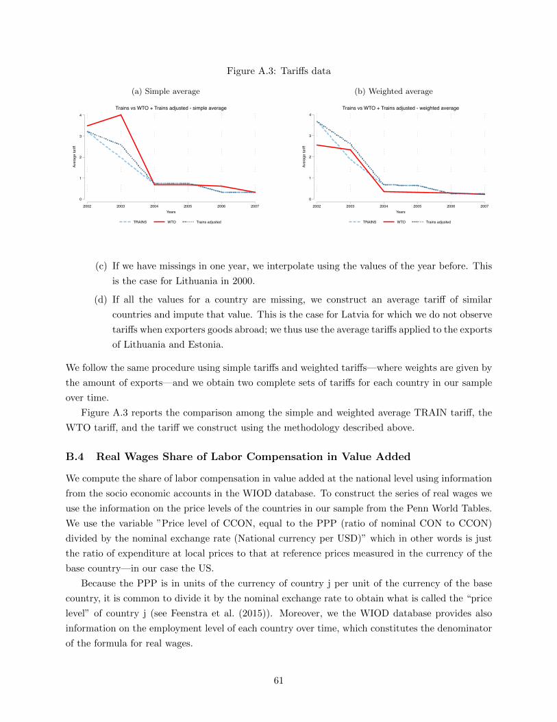
Figure A.3: Tari↵s data

(a) Simple average

0

1

2

3

4

Aver

age

tarif

f

2002 2003 2004 2005 2006 2007Years

TRAINS WTO Trains adjusted

Trains vs WTO + Trains adjusted - simple average

(b) Weighted average

0

1

2

3

4

Aver

age

tarif

f

2002 2003 2004 2005 2006 2007Years

TRAINS WTO Trains adjusted

Trains vs WTO + Trains adjusted - weighted average

(c) If we have missings in one year, we interpolate using the values of the year before. This

is the case for Lithuania in 2000.

(d) If all the values for a country are missing, we construct an average tari↵ of similar

countries and impute that value. This is the case for Latvia for which we do not observe

tari↵s when exporters goods abroad; we thus use the average tari↵s applied to the exports

of Lithuania and Estonia.

We follow the same procedure using simple tari↵s and weighted tari↵s—where weights are given by

the amount of exports—and we obtain two complete sets of tari↵s for each country in our sample

over time.

Figure A.3 reports the comparison among the simple and weighted average TRAIN tari↵, the

WTO tari↵, and the tari↵ we construct using the methodology described above.

B.4 Real Wages Share of Labor Compensation in Value Added

We compute the share of labor compensation in value added at the national level using information

from the socio economic accounts in the WIOD database. To construct the series of real wages we

use the information on the price levels of the countries in our sample from the Penn World Tables.

We use the variable ”Price level of CCON, equal to the PPP (ratio of nominal CON to CCON)

divided by the nominal exchange rate (National currency per USD)” which in other words is just

the ratio of expenditure at local prices to that at reference prices measured in the currency of the

base country—in our case the US.

Because the PPP is in units of the currency of country j per unit of the currency of the base

country, it is common to divide it by the nominal exchange rate to obtain what is called the “price

level” of country j (see Feenstra et al. (2015)). Moreover, we the WIOD database provides also

information on the employment level of each country over time, which constitutes the denominator

of the formula for real wages.

61

B.5 Portuguese Matched Employer-Employee Data

Employer-employee data come from Quadros de Pessoal, a longitudinal data set matching virtually

all firms and workers based in Portugal.58 Reported data cover the firm itself, as well as each of

its workers. Each firm and each worker entering the database are assigned a unique, time-invariant

identifying number which can be used to follow firms and workers over time.

Currently, the data set collects data on about 350,000 firms and 3 million employees. Each year,

every firm with wage earners is legally obliged to fill in a standardized questionnaire. Reported

data cover the firm itself, each of its plants, and each of its workers. The worker-level data cover

information on all personnel working for the reporting firms in a reference week. They include

information on gender, age, occupation, schooling, hiring date, earnings, hours worked (normal

and overtime), etc. The information on earnings includes the base wage (gross pay for normal

hours of work), seniority-indexed components of pay, other regularly paid components, overtime

work, and irregularly paid components.59 It does not include employer’s contributions to social

security.

The administrative nature of the data and their public availability at the workplace—as required

by the law—imply a high degree of coverage and reliability. The public availability requirement

facilitates the work of the services of the Ministry of Employment that monitor the compliance of

firms with the law (e.g., illegal work).

C Change in Migration Costs: Placebo Plots and Residual Cases

In Section 4.1, we described the methodology used to identify changes in migration costs for the

main events in our sample period: the United Kingdom opening to NMS countries in 2004, followed

by Greece, Italy, Spain, and Portugal in 2006, and NMS countries opening their respective labor

markets to each other and (mostly) to EU-15 countries in 2004. We also ran a number of placebo

experiments to support our identification strategy. In this appendix we provide additional support

for the identification strategy by showing, in sub-appendix C.1, a series of plots that allow to

evaluate the common trend assumption. Sub-appendix C.2 reports similar plots for the placebo

experiments.

62

Figure C.1: Log odds of migrating to the U.K. vs. staying in a NMS country for NMS nationals,treatment and control flows, 2002-2007

-35

-30

-25

-20

-15

-10

(Log

) rat

io o

f num

ber

of m

igra

nts

to s

taye

rs

2002 2003 2004 2005 2006 2007Year of emigration

Treatment: NMS8 to UK Control: NMS8 to EU5, and EU5 to UK

NMS nationals

Note: Treatment flows in solid red, control flows in dashed blue. The pink vertical dashed line marks thebeginning of the treatment period.

C.1 Common Trend Assumption

Figure C.1 shows the evolution over time of the (log) odds of migrating vs. staying (equation 10)

for the treated and control groups of NMS nationals. The treated group is represented by the NMS

to U.K. flow of NMS nationals, with the treatment period being after 2003. The control group is

represented by the NMS to EU-5 and EU-5 to U.K. flows of NMS nationals. The figure clearly

conveys two messages: First the odds for both the treated and control groups were increasing

before the 2004 enlargement; second, when comparing the pre-treatment and treatment periods,

the change in the odds of migrating is clearly positive for the treated group and close to zero for

the control group. These patterns are consistent with a substantial reduction in migration costs

from NMS to the United Kingdom.

Turning to the southern European destinations, Figure C.2 reports the evolution of the (log)

odds for Greece, Italy, Spain, and Portugal—with the treatment period being after 2005. Overall,

the comparison between the log odds of the treatment and the control groups before the policy

58Public administration and non-market services are excluded. Quadros de Pessoal has been used by, among others,\cite{Cabral03} to study the evolution of the firm size distribution; by \cite{Blanchard01} to compare the U.S. andPortuguese labor markets in terms of unemployment duration and worker flows; by \cite{Cardoso05} to study thedeterminants of both the contractual wage and the wage cushion (di↵erence between contractual and actual wages);by \cite{Carneiro12} who, in a related study, analyze how wages of newly hired workers and of existing employeesreact di↵erently to the business cycle; by \cite{Martins09c} to study the e↵ect of employment protection on workerflows and firm performance. See these papers also for a description of the peculiar features of the Portuguese labormarket.

59It is well known that employer-reported wage information is subject to less measurement error than worker-reported data. Furthermore, the Quadros de Pessoal registry is routinely used by the inspectors of the Ministry ofEmployment to monitor whether the firm wage policy complies with the law.

63

Figure C.2: Log odds of migrating to Greece/Italy/Spain/Portugal vs. staying in a NMS countryfor NMS nationals, treatment and control flows, 2002-2007

(a) Greece

-35

-30

-25

-20

-15

-10

(Log

) rat

io o

f num

ber

of m

igra

nts

to s

taye

rs

2002 2003 2004 2005 2006 2007Year of emigration

Treatment: NMS8 to GR Control: NMS8 to EU5, and EU5 to GR

NMS nationals

(b) Italy

-35

-30

-25

-20

-15

-10

(Log

) rat

io o

f num

ber

of m

igra

nts

to s

taye

rs

2002 2003 2004 2005 2006 2007Year of emigration

Treatment: NMS8 to IT Control: NMS8 to EU5, and EU5 to IT

NMS nationals

(c) Spain

-35

-30

-25

-20

-15

-10

(Log

) rat

io o

f num

ber

of m

igra

nts

to s

taye

rs

2002 2003 2004 2005 2006 2007Year of emigration

Treatment: NMS8 to ES Control: NMS8 to EU5, and EU5 to ES

NMS nationals

(d) Portugal

-35

-30

-25

-20

-15

-10(L

og) r

atio

of n

umbe

rof

mig

rant

s to

sta

yers

2002 2003 2004 2005 2006 2007Year of emigration

Treatment: NMS8 to PT Control: NMS8 to EU5, and EU5 to PT

NMS nationals

Note: Treatment flows in solid red, control flows in dashed blue. The pink vertical dashed line marks thebeginning of the treatment period.

changes confirms that the control groups represent a good measure of counterfactual log odds in

the absence of a policy change. Except for the case of Greece, the odds of migrating vs. staying de-

creases, from the pre-treatment to the treatment period, both for the control and the treated groups

but significantly less for the latter, pointing to a positive contribution associated to a reduction in

migration costs.

C.2 Placebo Experiment

As shown in Section 2.1, a placebo experiment confirms the prior that EU nationals did not expe-

rience any significant change in the cost of migrating back to Europe from NMS countries. Figure

C.3 reports the evolution of the (log) odds for the treated and control groups.

64

Figure C.3: Log odds of migrating vs. staying for EU nationals (Placebo), from NMS countries toGreece/Italy/Spain/Portugal, treatment and control, 2002-2007

(a) Greece

-35

-30

-25

-20

-15

-10

(Log

) rat

io o

f num

ber

of m

igra

nts

to s

taye

rs

2002 2003 2004 2005 2006 2007Year of emigration

Treatment: NMS8 to ES Control: NMS8 to EU5, and EU5 to ES

EU nationals

(b) Italy

-35

-30

-25

-20

-15

-10

(Log

) rat

io o

f num

ber

of m

igra

nts

to s

taye

rs

2002 2003 2004 2005 2006 2007Year of emigration

Treatment: NMS8 to IT Control: NMS8 to EU5, and EU5 to IT

EU nationals

(c) Spain

-35

-30

-25

-20

-15

-10

(Log

) rat

io o

f num

ber

of m

igra

nts

to s

taye

rs

2002 2003 2004 2005 2006 2007Year of emigration

Treatment: NMS8 to ES Control: NMS8 to EU5, and EU5 to ES

EU nationals

(d) Portugal

-35

-30

-25

-20

-15

-10(L

og) r

atio

of n

umbe

rof

mig

rant

s to

sta

yers

2002 2003 2004 2005 2006 2007Year of emigration

Treatment: NMS8 to PT Control: NMS8 to EU5, and EU5 to PT

EU nationals

Note: Treatment flows in solid red, control flows in dashed blue. The pink vertical dashed line marks thebeginning of the treatment period.

D International Migration Elasticity

In this appendix we describe in detail the estimation method used to find the international migration

elasticity in Section 4.2. We estimate the international migration elasticity, 1/⌫, by adapting the

method presented in Artuc and McLaren (2015) to our theory and data. The method has two

stages: first the Poisson regression stage where we estimate value di↵erences and the migration

cost function, normalized by ⌫, for every time period. Second, the Bellman equation stage, where

we insert the estimated value di↵erences into a Bellman equation and construct a linear regression

to retrieve the international migration elasticity, 1/⌫.60

The estimation method relies on the following two equilibrium conditions from the model: the

60Since we estimate the elasticity using only flows of EU nationals within EU-15 we drop the n subscript.

65

migration share equation

µijt,s =

h

exp⇣

�V jt+1,s �mij

t,s

⌘i

1/⌫

PNk=1

h

exp⇣

�V kt+1,s �mik

t,s

⌘i

1/⌫, (18)

and the Bellman equation

V it,s = log

�

Cit,s

�

+ ⌫ logh

PNk=1

⇥

exp�

�V kt+1,s �mik

t,s

�⇤

1/⌫i

=

= log�

wit,s/P

it

�

+ �EtV it+1,s + ⌦i

t,s,(19)

where

Cit,s =

wit,s

P it

is the consumption aggregator, and

⌦it,s = ⌫ log

XN

k=1

h

exp⇣

�⇣

V kt+1,s � V i

t+1,s

⌘

�mikt,s

⌘i

1/⌫

is the option value of migration.

First stage: Poisson regression The first stage is a fixed-e↵ect estimation—based on the

migration share equation and bilateral gross migration flows data—to estimate value di↵erences

and the migration cost function normalized by ⌫.

The estimating equation can be derived as follows. In the migration share equation (18),

multiply both numerator and denominator on the right hand side by⇥

exp�

��V it+1,s

�⇤

1/⌫,

µijt,s =

h

exp⇣

�⇣

V jt+1,s � V i

t+1,s

⌘

�mijt,s

⌘i

1/⌫

PNk=1

h

exp⇣

�⇣

V kt+1,s � V i

t+1,s

⌘

�mikt,s

⌘i

1/⌫.

Then multiply both sides by the mass of agents Lit,s,

Lit,sµ

ijt,s =

h

exp⇣

�⇣

V jt+1,s � V i

t+1,s

⌘

�mijt,s

⌘i

1/⌫

PNk=1

h

exp⇣

�⇣

V kt+1,s � V i

t+1,s

⌘

�mikt,s

⌘i

1/⌫Lit,s,

and rewrite as

Lit,sµ

ijt,s = exp

✓

�

⌫V jt+1,s �

�

⌫V it+1,s �

1

⌫mij

t,s + logLit,s �

1

⌫⌦it,s

◆

. (20)

We interpret the equation above as Poisson pseudo-maximum likelihood. The first stage regres-

sion is then

Zijt,s = exp

✓

�jt,s + ↵i

t,s �1

⌫mij

t,s

◆

+ "ijt,s, (21)

66

where Zijt,s = Li

t,sµijt,s asymptotically is the mass of agents with skill s moving from i to j in t, �j

t,s

is a destination-skill-time fixed e↵ect, ↵it,s is an origin-skill-time fixed e↵ect.

The estimation of (21) can be done pooling the observations associated to all years and skills

in the data. Since we estimate the migration elasticity using only flows of EU nationals within

EU-15 we assume that bilateral migration costs do not vary over time and skills, that is mijt,s = mij

for all {t, s} pairs. Note, however, that the cost of migrating out of country i, and into country j,

is still potentially skill-dependent because of ↵it,s, and �j

t,s, respectively. Finally, "ijt,s is a random

disturbance of relative migration costs.

The �jt,s and ↵i

t,s terms are not separately identified, so without loss of generality we set �1

t,s = 0

(or equivalently choose cell �1

t,s as the omitted category for the fixed e↵ects). Similarly, not all mij

are separately identified, so without loss of generality we set all mi,1 and m1j to zero. Overall, this

is equivalent to defining the destination-skill-time fixed e↵ects as

�jt,s =

�

⌫

⇣

EtVjt+1,s � EtV

1

t+1,s

⌘

� 1

⌫m1j , (22)

and the origin-skill-time fixed e↵ects as

↵it,s = ��

⌫

�

EtVit+1,s � EtV

1

t+1,s

�

+ logLit,s �

1

⌫⌦it,s �

1

⌫mi,1.

Note that the migration option value for an agent with skill s living in country i in year t can

be written as1

⌫⌦it,s = ��i

t,s � ↵it,s + logLi

t,s �1

⌫

�

mi,1 �m1j�

. (23)

Analogously to Silva and Tenreyro (2006), we use Poisson Pseudo Maximum Likelihood (PPML)

to estimate equation (21). This implies that, if we write the estimating equation (21) in the form

W ijt,s = exp

⇣

xijt,s�t,s⌘

+ "ijt,s, where xijt,s is a vector of dummy variables and �t,s is the vector of

parameters to be estimated, then we choose the parameters to solve the first-order condition

X

t

X

ij

h

W ijt,s � exp

⇣

xijt,s�t,s⌘i

xijt,s = 0.

Second stage: Bellman equation In stage 1 we have estimated the destination-skill-time and

origin-skill-time fixed e↵ects �jt,s and ↵i

t,s. The second stage rewrites the Bellman equation (19) as

an estimating equation using the estimated values from the first stage.

Using (19), we can write

�

⌫EtV

it+1,s =

�

⌫

log

✓

wi

t+1,s

P i

t+1

◆

+ �EtV it+2,s + ⌦i

t+1,s

�

.

Using (23) to substitute out the continuation value ⌦it+1,s, and using the expression for the

67

Table D.1: International Migration Elasticity, Second Stage Estimates

Baseline With public good

1/⌫0.44∗∗∗

(0.13)

0.53∗∗∗

(0.14)

Obs. 100 100Notes: Standard errors clustered at the

country-level in parentheses. ⇤⇤⇤ p<0.01

destination-skill-time fixed e↵ects (22), we get

�it,s +

�⌫EtV 1

t+1,s +1

⌫m1,i = �

⌫ log

✓

wi

t+1,s

P i

t+1

◆

+�2

⌫ EtV 1

t+2,s � �↵it+1,s + � logLi

t+1,s ��⌫

�

mi,1 �m1,i�

.(24)

Define

�it,s = �i

t,s + �↵it+1,s � � logLi

t+1,s, (25)

and

⇠t,s =�2

⌫EtV

1

t+2,s ��

⌫EtV

1

t+1,s,

and rewrite (24) as

�it,s = ⇠t,s + i +

�

⌫log

wit+1,s

P it+1

!

+ ✏it,s, (26)

where �it,s is the dependent variable constructed from Stage 1 estimates using (25), ⇠t,s is a time-

skill dummy, i = � (�/⌫)�

mi,1 �m1,i�

is a country fixed e↵ect, and ✏it,s is the regression residual.

The remaining right hand-side variables are all taken from the data: log�

wit+1,s/P

it+1

�

is the (log)

real wage; log�

Lit+1

�

is the lead of the (log) population in country i. We estimate (26) as an

IV regression, using two-period lagged values of real wages as instruments similar to Artuc et al.

(2010), and clustering standard errors at the country level.

We build wages, for each country i and year t 2 [2002� 2009], as the ratio of the economy-wide

“Labour compensation” (in millions of national currency) and “Number of persons engaged” (in

thousands) from the WIOD Socio-Economic Accounts (SEA) data set (Timmer et al. (2015b)).

Then, we use the purchasing-power-parity adjusted real exchange rate from version 9.0 of the Penn

World Tables to compare wages across countries and time (Feenstra et al. (2015)). To compute

wages by skill level we resort once again to the WIOD Socio-Economic Accounts: The high-skilled

wage is computed by applying the high-skilled share of labor compensation and the high-skilled

share of total hours; we convert hours into persons by assuming that the number of hours per

person does not vary with skills.

Table (D.1) reports the second stage IV estimates for 1/⌫ for � = 0.97 for the baseline case

and for the extension with public good described below. The estimates for alternative values of

� = {0.90, 0.95} are the same up to the second decimal digit.

68

D.1 Estimation with Public Goods

In section 5.2.2 of the main text we extended our model to account for additional congestion e↵ects

coming from the provision of public goods. It turns out that this extension only slightly modifies the

methodology for the estimation of the international migration elasticity outlined above. The first

stage, based on the migration share equation, is unchanged. The second stage relies on a modified

Bellman equation that includes the per capita provision of public goods�

Gi/Lit+1

�

, weighted by

the fraction of public goods in total consumption (↵i ), as well as wages net of labor income taxes,

�

⌫EtV

it+1,s =

�

⌫

8

<

:

↵i log�

Gi/Lit+1

�

+ (1� ↵i) log

�

1� ⌧ it+1

� wi

t+1,s

P i

t+1

�

+�EtV it+2,s + ⌦i

t+1,s

9

=

;

.

Following the same steps outlined above for the case without public good, it is easy to obtain the

estimating equation

�it,s = ⇠t,s + i +

�

⌫

(

�↵i logLit+1

+ (1� ↵i) log

"

�

1� ⌧ it+1

� wit+1,s

P it+1

#)

+ ✏it,s, (27)

where the country fixed e↵ect is now defined as i = (�/⌫)↵i logGi � (�/⌫)�

mi,1 �m1,i�

. In

terms of data, we need to compute the fraction of public goods in total consumption ↵i, which we

construct using the WIODWorld Input-Output Database, and we need information on labor income

taxes. In order to compute net real wages we resort to the OECD Tax Database, which provides

data on combined central and sub-central government income tax plus employee social security

contribution, as a percentage of gross wage earnings, for people whose income is 100 percent of

the average wage (OECD (2016)). In the OECD Tax Database the average wage is defined as the

average annual gross wage earnings of adult, full-time, manual and non-manual workers. Data are

available for each year for 14 countries in our sample, all except Lithuania, Latvia and Cyprus. For

these three countries we compute the tax rate as the average of the tax rate for all the other NMS

countries, by year.

E Elasticity of Substitution Between Low- and High-SkilledWork-

ers

In Section 4.3 we provided an estimate of the elasticity of substitution between low and high-skilled

workers. To construct the data, we consider all industries in the economy except for agriculture

and fishing, international organizations, and government and justice. We consider all single-job

workers between 18 and 65 years old, working no more than 480 hours per month, earning at least

the minimum wage, excluding apprentices and workers for which no information on education is

available. We trim the top and bottom 1 percent of workers according to the distribution of hourly

wages in each year. We end up with 25.7 millions observations that we aggregate into skill-year

69

groups to construct hours. To construct the average wage in each cell we use a more selective

sample that includes only employees with a permanent contract, working at least 35 hours per

week. The average weekly wage in a skill-year cell is constructed by using only the base wage, and

then taking the weighted average over workers where the weights are the regular hours worked by

the individual. Wages are deflated to 2005 using Statistics Portugal monthly consumer price index

by special aggregates that we convert to annual. In order to classify workers as “displaced” we

partly follow Carneiro and Portugal (2006) and define a firm as shutting down after year t when

the firm is observed in the Quadros de Pessoal data in year t but is not observed in the dataset

in any of the three subsequent years. If a firm is last active in t we record the total regular hours

worked by its low- and high-skilled workers in t and use these hours to construct the instrument

for t+ 1.61

Table E.1 reports the estimates, which are all significant at 1 percent. Employing the IV

methodology and data outlined above, we obtain an elasticity of 4, which is the number we use in

our quantitative analysis. Our estimate is slightly above those commonly found for the U.S. (Katz

and Murphy (1992); Johnson (1997); Krusell et al. (2000); Ottaviano and Peri (2012); Ciccone and

Peri (2005)) which range between 1.5 and 2.5, but below the elasticity of substitution of 5 between

low- and medium-skilled workers found for Germany (Dustmann et al. (2009)). Since the set of

European countries we consider in the quantitative analysis is pretty diverse in terms of labor

market institutions and workforce characteristics we consider our benchmark estimate of 4 as a

good compromise.

The estimate of the elasticity of substitution turns out to be pretty robust to alternative di↵erent

specifications, methodologies, and levels of data aggregation. Table E.1 reports an alternative set

of estimates using OLS with linear or spline (with break in 1993) trends, at the industry-region and

country-level. It also reports a set of estimates based on an alternative way to construct the data

series for hours and wages based on Autor et al. (2008). In this case we construct a fix-weighted ratio

of high-skill to low-skill wages for a composition-constant set of sex-education-experience groups.

To do that, we regress monthly deflated wages, for each sex and year, on five education categories

(3 years or less, between 4 and 6 years, between 7 and 9 years, between 10 and 12 years, and 13

years and above), a quartic in experience (defined as age minus 6 minus the number of education

years), and all the interactions between the education dummies and the quartic in experience. The

predicted wages for each sex-education-experience-year group are then aggregated at the skill-year

level with a constant set of weights based on the aggregate hours shares of each group. The series

for hours is constructed by aggregating at the skill-year level the series for total regular hours

worked by sex, five education groups and experience. The aggregation employs a series of weights

to turn hours into e�ciency units. Weights are constructed by normalizing the predicted wages

described above by the top wage across cells. Estimates for the elasticity of substitution, using

di↵erent types of trends turn out to be slightly smaller, but overall pretty similar to all the others.

61We construct the lead because the information reported in Quadros de Pessoal is collected in October of everyyear from 1994 on (before that it was collected in March).

70

Table E.1: Elasticity of substitution between low- and high-skill workers, Portuguese matchedemployer-employee data

Industry-region-level Country-levelCountry-level

(composition-adjusted)

Elasticity R2 Obs. Elasticity R2 Obs. Elasticity R2 Obs.IV 4.0 0.84 180

Linear trend 5.2 0.94 210 4.2 0.97 14 3.6 0.97 14

Spline 3.7 0.92 210 3.1 0.98 14 3.0 0.99 14

Note: All estimates are significant at 1 percent. All industry-region-level estimates include industry-regionfixed e↵ects. Industry-region-level OLS estimates include industry-region-specific trends.

F Equilibrium Conditions of the Temporary Equilibrium in Changes

In this appendix, we describe the equilibrium conditions of the production structure in relative time

di↵erences. As in the main text, let yt+1

⌘ yt+1

/yt denote the relative time change of a variable

and by yt+1

⌘ y0t+1

/yt+1

the relative time di↵erence of the variable under a sequence of policies

{⌥ 0t}1t=0

relative to the sequence of policies {⌥t}1t=0

. Also, let’s define !s,t = ws,t (rt)�i/(1��i).

The cost of the bundle of inputs and the price index in relative time di↵erences are

xit =

0

B

@

⇠0ih,t�1

⇣

!0ih,t

⌘

1�⇢+ ⇠

0il,t�1

⇣

!0il,t

⌘

1�⇢

⇠ih,t�1

⇣

!ih,t

⌘

1�⇢+ ⇠il,t�1

⇣

!il,t

⌘

1�⇢

1

C

A

(1��

i)1�⇢

,

P it =

✓

XN

j=1

⇡0ijt�1

⇡ijt A

jt (

ijt x

jt )

�✓

◆� 1✓

,

while the bilateral expenditure shares in relative time di↵erences are

⇡ijt =

ijt xjt

P it

!�✓

Ajt .

The share of high-skilled labor in the counterfactual equilibrium is given by

⇠i0s,t = ⇠is,t�1

⇣

!0is,t

⌘

1�⇢

�

x0it

�

1�⇢

1��

i

.

Total expenditure in the counterfactual equilibrium is given by

X0it = ⌅

�

!0h,t

�

1��i

⇣

⇠0ih,t

⌘�i ⇣

L0ih,t

⌘

1��i

w0ih,t�1

L0ih,t�1

+�

!0l,t

�

1��i

⇣

⇠0il,t

⌘�i ⇣

L0il,t

⌘

1��i

w0il,t�1

L0il,t�1

+ ◆i�0t,

71

with ⌅ = 1

PN

j=1⇡

0ij

t

(1+⌧

0ij

t

)

and �0t =

PNi=1

⇣

!0ih,t

⌘

✓

˙L0i

h,t

˙⇠0i

h,t

◆

1��

rit�1

H i.

Finally, the labor market condition of high-skilled labor is

!0is,t =

0

B

@

1⇣

⇠0is,t

⌘�i

⇣

L0is,t

⌘

1��i

(1� �i)⇠0is,t

w0is,t�1

L0is,t�1

XN

j=1

⇡0jit X

0jt

⌧0jit

!

1

C

A

11��

i

.

72