golf ball dynamics

8/3/2019 Golf Ball Dynamics

http://slidepdf.com/reader/full/golf-ball-dynamics 1/16

Golf Ball Flight Dynamics

James Barber III

Cornell University

A&EP 434 Final Project

Professor Lovelace



Contents

Introduction . . . . . . . . . . . . . . . . . . . . . . . . . . . . . . . . . . . . . . . . . . . . 1

Terminology . . . . . . . . . . . . . . . . . . . . . . . . . . . . . . . . . . . . . . . . . 2Idealizing a Golf Ball: Playing with a Smooth Sphere . . . . . . . . . . . . . . . . . . . . 3

Introduction . . . . . . . . . . . . . . . . . . . . . . . . . . . . . . . . . . . . . . . . . 3The Model . . . . . . . . . . . . . . . . . . . . . . . . . . . . . . . . . . . . . . . . . 3Results . . . . . . . . . . . . . . . . . . . . . . . . . . . . . . . . . . . . . . . . . . . . 5

T h e E ff e c t s o f D i m p l e s . . . . . . . . . . . . . . . . . . . . . . . . . . . . . . . . . . . . . . 5Introduction . . . . . . . . . . . . . . . . . . . . . . . . . . . . . . . . . . . . . . . . . 5The Effect of an Additional Lift Term . . . . . . . . . . . . . . . . . . . . . . . . . . 6The Effect of Reduced Drag . . . . . . . . . . . . . . . . . . . . . . . . . . . . . . . . 7

Conclusion . . . . . . . . . . . . . . . . . . . . . . . . . . . . . . . . . . . . . . . . . . . . 10Appendix A - Constants Used for Numerical Calculations . . . . . . . . . . . . . . . . . . 11

Appendix B - Mathematica Code used to Model Ball Flights . . . . . . . . . . . . . . . . 12Bibliography . . . . . . . . . . . . . . . . . . . . . . . . . . . . . . . . . . . . . . . . . . . 14



James Barber III Golf Ball Flight Dynamics 1

Introduction

Although poorly documented, golf is believed to have originated in Scotland in 1456[1]. It wasfirst played as a very casual game for which no standard rules existed. A wooden ball was usedin conjunction with wooden clubs prior to 1618[2], when the “featherie” (a ball made of stitchedleather and tightly packed with feathers) was introduced. The featherie was favored for its moreforgiving feel on the hands of players when it was struck and was used until 1848 when the inventionof the “Gutta” surpassed the “featherie” in both durability and cost. The “Gutta” was made of gutta-percha packing material which was not brittle and became soft and moldable at 100

° C.

The Gutta’s pliability made it necessary to roll the ball on a “smoothing board” in order to

maintain its shape and keep it free of imperfections which were created during normal play of thegame. The smooth Gutta was used for only a few years before players began to realize that ballsthat had not been well maintained and had many nicks and scratches had a much more favorableflight. Thus began the practice of hammering the Gutta with a sharp-edged hammer in a regularpattern to increase the consistency of the ball’s play.

In 1898 the first “Balata” ball was created by wrapping rubber thread around a solid rubbercore which was then covered by a solid layer of rubber that later became known as the “ball cover”.The Balata was the first sign of a modern age of golf technology for it allowed molds to be used tocreate consistent cover patterns. In 1908 makers discovered the superiority of a regular “dimple”pattern over the haphazard grid pattern favored by players at the time.

Dimples are small indentations on the exterior of the golf ball. They are typically round in shapeand vary in diameter from 2-5mm in diameter and are about .2mm deep. Modern golf balls packanywhere from 300-450 dimples of varying size arranged in a regular pattern on the outside of everyball[3]. Dimples have been one of the most influential developments in golf ball design because theyalter the dynamics of the balls flight in such a way that gives golfers a significant amount of controlover the height and shape of their shots.

Today, golf balls are highly regulated by the United States Golf Association (USGA) for com-pliance with rules governing the design and capabilities of a golf ball. Modern materials, such asSurlyn and Urethane as well is different core designs, have given ball designers the ability to create

golf balls with almost any property desired (higher spin, softer feel at impact, lower trajectory,etc...). It is well known that due to the complexities involved with the aerodynamics of a golf ball,ball designers have taken a “design, test, and modify” approach to ball design as an alternative tocomputer modeling and CAD techniques.

In this paper I investigate a recent mathematical derivation for the aerodynamics of a smoothsphere and attempt to extend it to golf balls by incorporating the effects of dimples on air flowand comparing the results of simulations to observations taken from modern professional golfers.Although this technique will hopefully one day lead to the derivation of equations governing theflight of balls with arbitrary dimple patterns in pursuit of optimizing dimple design for maximumdistance, the scope of this paper is limited to comparing two key effects that dimples have on ball

flight.




Terminology

Golfers use a significant vocabulary that may not be recognized by those unfamiliar with the game.This section gives an introduction to basic terminology that will be used throughout this document.

Loft - The angle between the club face and the shaft. The more loft a club has, the higher it willlaunch the ball at impact.

Figure 1: Loft[4]

Impact - The instant in time when a player strikes the ball with the club.

Ball flight - The path a ball takes after impact, while it is in the air. There are also two broadtypes of shot shapes : a hook and a slice, and two directional descriptors: a pull and a push . Ahook is a ball flight in which the ball curves from right to left due to a small amount of side-spin being imparted to it at impact. Similarly, a slice is a ball flight in which the ball curvesfrom left to right, due to sidespin imparted to the ball at impact in the opposite direction fromthe hook result. A pull is when the ball starts its path to the left of its intended destination.Likewise, push is when the ball starts its path to the right of its intended destination. Pleasenote that each of these terms is defined for a player using “right-handed” clubs, and changesits meaning if the player uses left-handed clubs.

Figure 2: Ball Flights[5]

Carry - The distance a ball travels in the air, after being struck. Note that this excludes thedistance that the ball bounces and rolls after it first strikes the ground (this is called roll ).




Idealizing a Golf Ball: Playing with a Smooth Sphere

Introduction

A golf ball is a sphere about 4.2cm in diameter, with hundreds of small niches (dimples) carved inits outer face. While the dimples play a key role in the flight dynamics of the ball, I refrain fromcovering their effects until the next section. In this section we use a complex mathematical modelderived and published by Karl I. Borg[6] in 2003 to model the flight of a golf ball under conditionstypical for a professional golfer when striking the ball with a driver (see table 1). While this modelis intended for use at low Reynolds Numbers, it has been experimentally shown to be reasonable aswell for higher Reynolds Numbers. The Reynolds Number is a quantity that indicates the relative

importance of inertial forces compared to viscous forces in determining its path through a gas orfluid. High Reynolds Numbers indicate that viscous forces are less important.

Re =d · V ν

(1)

Equation (1) is used to compute the Reynolds Number (Re), where d is the diameter of the object,V is the objects velocity, and ν is kinematic viscosity of the fluid or gas, given by (2),

ν =µ

ρ(2)

where µ is the Absolute Viscosity of the fluid or gas (fixed value for a given compound) and ρ isits density. For a golf ball flying through 68◦F air at sea level, the associated Reynolds Numberfalls in the range of 2.15x105 to 9.0x104, which means that viscosity is much less important thanthe ball’s inertia.

The Model

Borg’s model incorporates drag, heat exchange between the gas and the sphere (ball), and theMagnus Effect. The Magnus Effect (occasionally referred to as the Robins Effect for spheres) is alift force that results from the rotation of a cylinder or sphere as it moves through a fluid or gasand was first described by German physicist Heinrich Magnus in 1853[7]. The lift force occurs as

a result of spin creating a region of lower pressure above a ball with backspin (due to Bernoulli’sPrinciple). The net force on the sphere as derived by Borg et al is given by (3)

F = −ατ π12 pR2

πm

2kBT χ(z) v − ατ ξ

2

3πR3mn ω × v − ατ

1

3πR3mnχ

(z)

| ω| ω × ( ω × v) (3)

where ατ is the accommodation coefficient of tangential momentum (fraction of reflected gas par-ticles that are reflected diffusely), R is the radius of the sphere, m is mass of a single molecule of the gas, kT is Boltzmann’s Constant, T is the temperature of the gas, ω is the angular velocityof sphere’s rotation, v is the velocity of the sphere, and p, χ, z, and ξ are given by equations (4)through (8)




p = nkBT (4)

χ = ατ nkBT

κ

kBT

2πm(5)

B =1 − i√

2

| ω|R2

k(6)

z =j1(B)

χj1(B) + Bj 1

(B)(7)

ξ = 1 − χ

4

(z) +

2πkBT m

(z)4| ω|R

(8)

where n is the number density of the gas, κ is the heat conductivity of the sphere, j1 are thespherical Bessel functions of the first kind (with j

1its derivative), i =

√−1, and k is given by

k =κ

ρC p(9)

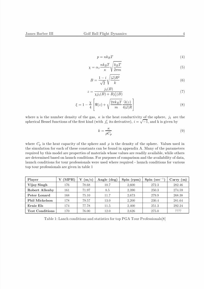
where C p is the heat capacity of the sphere and ρ is the density of the sphere. Values used inthe simulation for each of these constants can be found in appendix A. Many of the parameters

required by this model are properties of materials whose values are readily available, while othersare determined based on launch conditions. For purposes of comparison and the availability of data,launch conditions for tour professionals were used where required - launch conditions for varioustop tour professionals are given in table 1

Player V (MPH) V (m/s) Angle (deg) Spin (rpm) Spin (sec−1) Carry (m)

Vijay Singh 176 78.68 10.7 2,600 272.3 282.46

Robert Allenby 161 71.97 8.5 2,390 250.3 274.59

Peter Lonard 168 75.10 11.7 2,673 279.9 268.38

Phil Mickelson 178 79.57 13.0 2,200 230.4 281.64

Ernie Els 174 77.78 11.5 2,400 251.3 292.24

Test Conditions 170 76.00 12.0 2,626 275.0 ????

Table 1: Lanch conditions and statistics for top PGA Tour Professionals[8]




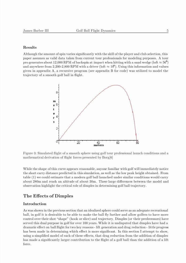
Results

Although the amount of spin varies significantly with the skill of the player and club selection, thispaper assumes as valid data taken from current tour professionals for modeling purposes. A tourpro generates about 12,000 RPM of backspin at impact when hitting with a sand wedge (loft ≈ 56

° )

and anywhere from 2,200-2,800 RPM with a driver (loft ≈ 10° ). Using this information and values

given in appendix A, a recursive program (see appendix B for code) was utilized to model thetrajectory of a smooth golf ball in flight.

Figure 3: Simulated flight of a smooth sphere using golf tour professional launch conditions and amathematical derivation of flight forces presented by Borg[6]

While the shape of this curve appears reasonable, anyone familiar with golf will immediately noticethe short carry distance predicted in this simulation, as well as the low peak height obtained. Fromtable (1) we could estimate that a modern golf ball launched under similar conditions would carryabout 280m and reach an altitude of about 30m. These large differences between the model and

observation highlight the critical role of dimples in determining golf ball trajectory.

The Effects of Dimples

Introduction

As was shown in the previous section that an idealized sphere could serve as an adequate recreationalball, in golf it is desirable to be able to make the ball fly further and allow golfers to have morecontrol over their shot “shape” (hook or slice) and trajectory. Dimples (or their predecessors) haveserved this dual purpose in golf for over 100 years. While it is undisputed that dimples have had adramatic effect on ball flight for two key reasons - lift generation and drag reduction - little progress

has been made in determining which effect is more significant. In this section I attempt to show,using a simplified model of each of these effects, that drag reduction from the addition of dimpleshas made a significantly larger contribution to the flight of a golf ball than the addition of a liftforce.




The Effect of an Additional Lift Term

Dimples generate a lift force on the golf ball because of the significant amount of backspin impartedto the ball at impact. This spin creates an asymmetry in the speeds at which air flows over thedimples in the top and bottom of the ball. Assuming the ball is traveling at velocity V 0 and theball is spinning with angular velocity ω, the air speeds relative to the top and bottom of the ballare given by (10)

V top = V 0 − ωR

V bottom = V 0 + ωR (10)

where R is the radius of ball. Since, in air, lift is proportional to velocity squared[9], this gives anet lift on the ball from the dimples of

Lift ∝ V 2bottom − V 2top = (V 0 + ωR)2 − (V 0 − ωR)2 = 4V 0ωR ∝ V 0ωR (11)

Using this relation and estimates of the lift coefficient (CL) in the range of 1.5x10−5 to 3.0x10−5 kg/m,the results in figure (4) were obtained when this term was incorporated into the existing model.

Figure 4: Simulated ball flight with the addition of a lift term

When this result is compared to the ball flight in the previous section without the lift term, it iseasy to see that the lift term did little to increase the distance that the ball traveled. It should benoted, however, that the lift term did make two important changes to the result: 1) the ball traveled

higher than without this term (≈9m at its peak), and 2) the ball stayed aloft for a significantlylonger period of time (4.9 seconds vs. 3.1 seconds without lift). The shape of this trajectory issimilar to that of a golf ball hit with more than an optimal amount of backspin - this shape isknown as a “blow up” in golf (figure 5). This simulation showed several encouraging signs thatseemed to indicate that the approximate lift force used gave realistic results.




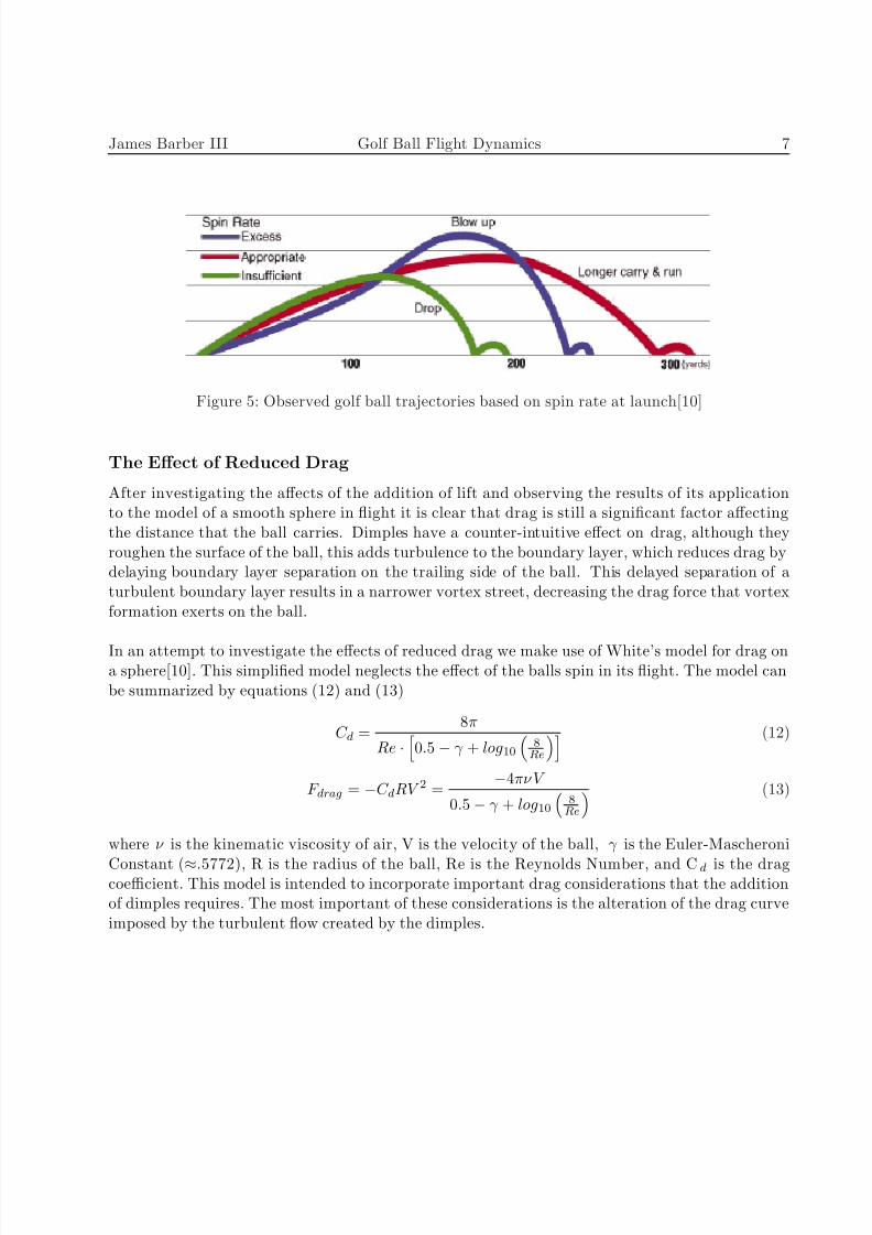
Figure 5: Observed golf ball trajectories based on spin rate at launch[10]

The Effect of Reduced Drag

After investigating the affects of the addition of lift and observing the results of its applicationto the model of a smooth sphere in flight it is clear that drag is still a significant factor affectingthe distance that the ball carries. Dimples have a counter-intuitive effect on drag, although theyroughen the surface of the ball, this adds turbulence to the boundary layer, which reduces drag bydelaying boundary layer separation on the trailing side of the ball. This delayed separation of aturbulent boundary layer results in a narrower vortex street, decreasing the drag force that vortexformation exerts on the ball.

In an attempt to investigate the effects of reduced drag we make use of White’s model for drag ona sphere[10]. This simplified model neglects the effect of the balls spin in its flight. The model canbe summarized by equations (12) and (13)

C d =8π

Re ·

0.5 − γ + log10

8

Re

(12)

F drag = −C dRV 2 =−4πνV

0.5− γ + log10

8

Re

(13)

where ν is the kinematic viscosity of air, V is the velocity of the ball, γ is the Euler-Mascheroni

Constant (≈.5772), R is the radius of the ball, Re is the Reynolds Number, and Cd is the dragcoefficient. This model is intended to incorporate important drag considerations that the additionof dimples requires. The most important of these considerations is the alteration of the drag curveimposed by the turbulent flow created by the dimples.




Figure 6: Flow modifications imposed by the addition of dimples[11]

This lowered Reynolds Number required for the transition to turbulent flow (steep drop in dragcoefficient) is necessary because even professionals are only able to give the golf ball an initialvelocity high enough to create a Reynolds Number of about 4x105, which would not quite reach thevalue required for the large drop in drag coefficient for a smooth sphere. With the dimples, however,a Reynolds Number of only 5x104 is necessary to achieve a significant drop in drag coefficient; thisvalue can be reached by a golf ball moving at just 8.9 m/s - a speed above which the ball travelsfor the entirety of its flight, thereby gaining maximum possible gains from the modified drag curve.

Figure 7: Simulated ball flight for a sphere with reduced drag

Several observations can be made from the results of the simulation using the simplified, reduceddrag model. First, the shape of the flight is much more ideal because the model neglects the effects

of spin on drag, and also excludes lift forces due to spin. The most dramatic difference to notice inthis simulation is large increase in carry (over 150m). This is most likely due to a higher velocitybeing maintained throughout the ball’s flight, which allows the ball to travel much further in thehorizontal direction in the same amount of time. It is also important to note that the maximumheight achieved is 60% (5 meters) higher than that of the smooth ball. While this is still quite farfrom the heights typical of actual golf balls (30m), it is not difficult to see the aggregate effects of the reduced drag and increased lift combining to yield a significantly higher peak height.




Combining the Effects of Additional Lift and Reduced Drag

Figure 8: Simulated ball flight for a sphere with reduced drag and an additional lift term

As a final exhibition, figure (8) represents a simulated golf ball flight by using both the reduced drag

force and the addition of a lift term. These two very simplistic force models combined harmoniouslyto produce a simulated ball flight with parameters that very nearly match observed values. Anunfortunate by-product of using the simplified drag model is loss of shape in the balls path. Thiseffect is noticeable when comparing the simplified drag model results (figures 7 & 8) to results fromusing Borg’s full drag equation (figures 3 & 4). Both the angle of impact as well as the speed of the ball at landing should be subject to scrutiny in this model. While the ball is moving at about37m/s just before it hits the ground in this model, observation has the ball impacting the ground at

just under 32m/s. It should be noted that this is a significant improvement (in terms of modelinga golf ball) over Borg’s model which predicts a smooth sphere to hit the ground at around 10m/s.




Conclusion

While it was clear that neither increasing the lift nor reducing the drag on the ball are enoughalone to change the trajectory to match what is observed in actuality, it is not difficult to see thatthe reduction in drag has a much larger effect on the trajectory of the ball. While Borg’s derivationof the forces on a smooth spinning sphere in flight is quite impressive and proves very successfulin modeling the flight of a smooth sphere, a significant amount of work remains to incorporate theeffects of dimples on the balls flight to a level where the model could be of use to ball designers.This appears to be a clear next step in the technological advancement of the golf industry. Whilepractical methods and designs have brought significant advances in ball technology, computers andmodern aerodynamic theory should allow for true optimization of golf ball design.




Appendix A - Constants Used for Numerical Calculations

ατ = accommodation coefficient of tangential momentum = 360◦−40

◦

360◦= 8

9

R = radius of the sphere (golf ball) = 2.13cm

m = mass of a single molecule of the gas (air, average) = 28.98 amu = 4.812 x 10 −26 kg

kB = Boltzmann’s Constant = 1.38 x 10−23 J ◦K

T = temperature of the gas (air) = 20◦C = 293.15◦K

ω = angular velocity of sphere’s rotation = 76 radsec

(at launch)

v = velocity of the sphere (golf ball) = 76 msec

cos

π15

,sin

π15

, 0

(at launch)

Launch angle = 12◦ = π15

radians

n = number density of the gas (air) = 2.503 x 1025moleculesm3

κ = heat conductivity of the sphere (assumed to be made of hard rubber) = 0.4 J m·sec·◦K

C p = heat capacity of the sphere = 124 cal◦K = 519.16 J

◦K

ρ = density of the gas (air) at 20◦C and 1 atm = 1.2047 kgm3

µ = Absolute Viscosity of the gas (air) = 1.82 x 10−5 kgm·sec




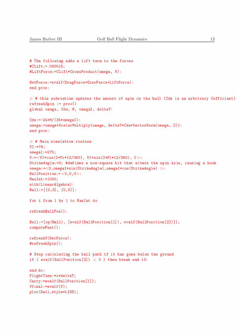
Appendix B - Mathematica Code used to Model Ball Flights

>with(LinearAlgebra):

deltaT:=.01;

M:=.04593;

BallPosition:=<0,0,0>;

GravForce:=<0,-9.8*M,0>;

> with(LinearAlgebra):

B:=(1-I)*sqrt(VectorNorm(omega, 2)*(R2̂)/(2*k));

chi:=(alphaT*n*KB*T/kappa)*sqrt(KB*T/(2*Pi*m));

k:=kappa/(rho*Cp);z:=BesselJ(1,B)/(chi*BesselJ(1,B)+B*(BesselJ(0,B)-BesselJ(1,B)/B));

p:=n*KB*T;

xi:=1-(chi/4)*(Re(z)+sqrt(2*Pi*KB*T/m)*Im(z)/(4*VectorNorm(omega, 2)*R));

> refreshV := proc(Fnet)

global V, deltaT, M:

V:=V+ScalarMultiply(Fnet, deltaT/M):

end proc:

> refreshBallPos := proc()

global deltaT, V, BallPosition:BallPosition:=BallPosition+ScalarMultiply(V, deltaT):

end proc:

> computeFnet := proc()

global V, omega, GravForce, B, chi, z, xi, p, k, Force, DragForce, NetForce, LiftForce,

Clift, R, CD, nu:

R:=.04267/2:

nu:=.000015:

with(LinearAlgebra);

Force:=-alphaT*(Pi/12*p*R 2̂*sqrt(Pi*m/(2*KB*T))*chi*Re(z)*V-2/3*xi*Pi*R 3̂*m*n*

CrossProduct(omega, V)-Pi/3*R3̂*m*n*chi*Im(z)/VectorNorm(omega, 2)*

CrossProduct(omega, CrossProduct(omega, V))):

DragForce:=eval(Force, [alphaT=280/360, n=2.503e25, KB=1.38e-23, T=293.15,

R=.04267/2, m=4.812e-26, kappa=.4, rho=1.1347e6, Cp=519.16]):

#The following lines alter the drag force to a less precise model

#CD:=4*Pi*nu/(.5-.577215665+log10(4*nu/(R*VectorNorm(V, 2)))):

#DragForce:=ScalarMultiply(V, -CD):

#The following lines alter the drag force to the most basic model (CD=const.)

#CD:=.29;

#DragForce:=ScalarMultiply(V, -CD*R):

LiftForce:=<0,0,0>:




# The following adds a lift term to the forces

#Clift:=.000015;

#LiftForce:=Clift*CrossProduct(omega, V):

NetForce:=evalf(DragForce+GravForce+LiftForce):

end proc:

> # this subroutine updates the amount of spin on the ball (Cds is an arbitrary Cefficient)

refreshSpin := proc()

global omega, Cds, M, omegaI, deltaT:

Cds:=-24*M/(35*omegaI):

omega:=omega+ScalarMultiply(omega, deltaT*Cds*VectorNorm(omega, 2)):

end proc:

> # Main simulation routine

VI:=76;

omegaI:=275;

V:=<VI*cos(2*Pi*12/360), VI*sin(2*Pi*12/360), 0>:

StrikeAngle:=0; #defines a non-square hit that alters the spin axis, causing a hook

omega:=<0,omegaI*sin(StrikeAngle),omegaI*cos(StrikeAngle) >:

BallPosition:=<0,0,0>:

MaxInt:=1000;

with(LinearAlgebra):

Ball:=[[0,0], [0,0]]:

for i from 1 by 1 to MaxInt do

refreshBallPos():

Ball:=[op(Ball), [evalf(BallPosition[1]), evalf(BallPosition[2])]];

computeFnet():

refreshV(NetForce):

#refreshSpin():

# Stop calculating the ball path if it has gone below the ground

if ( evalf(BallPosition[2]) < 0 ) then break end if:

end do:

FlightTime:=i*deltaT;

Carry:=evalf(BallPosition[1]);

Vfinal:=evalf(V);

plot(Ball,style=LINE);



Bibliography

[1] “Golf.” Encyclopedia Britannica. 2007. Encyclopedia Britannica Online. Available:

http://secure.britannica.com/eb/article-222218/golf. Accessed May 13, 2007.

[2] “History of Golf Balls.” Online. Available: http://www.golfjoy.com/golf physics/history.asp.Accessed 5/13/07.

[3] “Golf Ball.” Online. Available: http://en.wikipedia.org/wiki/Golf balls. Accessed 5/13/07.

[4] Original image obtained from: http://www.angelfire.com/pa/TWGOLF/fitinfo.html. Ac-cessed 5/13/07.

[5] Original image obtained from:http://golfdirt.com/cgi-bin/f.cgi?url=http://news.bbc.co.uk/sport2/hi/golf/skills/4245518.stm.

Accessed 5/13/07.

[6] Borg, Karl et al. “Forces on a spinning sphere moving in a rarefied gas.” Physics of FluidsVolume 15, Number 3 (March 2003): 736-41.

[7] Tritton, D.J. Physical Fluid Dynamics. Second Edition. Oxford: Clarendon Press, 1988.pp159-161.

[8] “Special Report: The Growing Gap.” Online. Available:http://www.golfdigest.com/equipment/index.ssf?/equipment/gd200305growinggap.html.Accessed: 5/9/07.

[9] Cross, Rod. “Ball Trajectories.” University of Sydney. August 1, 2006. Online. Avail-able: http://www.physics.usyd.edu.au/c̃ross/TRAJECTORIES/Trajectories.pdf. Accessed:5/11/07.

[10] White, Frank M. Viscous Flow. First edition. McGraw-Hill. Eqn. 2-265.

[11] “Flight Dynamics of Golf Balls.” Online. Available: http://www.golfjoy.com/golf physics/dynamics.asp.Accessed: 5/11/07.

golf ball dynamics

Documents