gmao annualreport09 jul14 · 2009research$highlights$ i$...
TRANSCRIPT

2009 Research Highlights
i
Global Modeling and Assimilation Office 2009 Research Highlights NASA Goddard Space Flight Center ★ June 30, 2010

Global Modeling and Assimilation Office
ii
The image on the front cover, courtesy of Bill Putman, is a comparison of clouds from the GOES satellite for 4-6 February 2010 and a GEOS-5 forecast at 5 km resolution, initialized 2 February.

2009 Research Highlights
iii
Table of Contents
The THORPEX Observation Impact Inter-‐comparison Experiment............................................1 Ronald Gelaro, Rolf Langland, Simon Pellerin, Ricardo Todling
Weak-‐Constraint Four-‐Dimensional Variational Atmospheric Data Assimilation......................3 Ricardo Todling, Banglin Zhang, Wei Gu, Ron Gelaro, Yannick Trémolet
Developing an Observing System Simulation Experiment Capability........................................5 Ronald Errico, Runhua Yang, Meta Sienkiewicz, Jing Guo, Ricardo Todling, Hui-Chun Liu
The Simulation of Doppler Wind Lidar Observations in Support of Future Instruments ...........7 Will McCarty, Ronald Errico, Runhua Yang, Ronald Gelaro
Aerosol Data Assimilation in GEOS-‐5.......................................................................................9 Arlindo da Silva, Ravi Govindaraju
Ocean Data Assimilation into the GEOS-‐5 Coupled Model with GMAO’s ODAS-‐2...................11 Christian Keppenne, Guillaume Vernieres, Michele Rienecker, Jossy Jacob, Robin Kovach
Assimilation of Satellite-‐derived Skin Temperature Observations into Land Surface Models .13 Rolf Reichle, Sujay Kumar, Sarith Mahanama, Randal Koster, Qing Liu
Toward Energetic Consistency in Data Assimilation...............................................................15 Stephen Cohn
Improved Simulation of Tropical Organization in GEOS-‐5 ......................................................17 Andrea Molod, Julio Bacmeister, Max Suarez
The GEOS-‐5 Coupled Atmosphere-‐Ocean Model ...................................................................19 Yury Vikhliaev, Max Suarez, Andrea Molod, Bin Zhao, Michele Rienecker
Cloud Parameterization using CRM Simulations and Satellite Data........................................21 Peter Norris, Arlindo da Silva, Lazaros Oreopoulos
The Impact of Altimetry and Argo data on GMAO’s Seasonal Forecasts.................................23 Michele Rienecker, Robin Kovach, Christian Keppenne, Jelena Marshak
Snow and Soil Moisture Contributions to Seasonal Streamflow Prediction............................25 Randy Koster, Sarith Mahanama, Ben Livneh, Dennis Lettenmaier, Rolf Reichle
Skill Assessment of a Spectral Ocean-‐Atmosphere Radiative Model ......................................27 Watson Gregg, Nancy Casey
Reanalyses: Metrics and Uncertainties..................................................................................30 Michael Bosilovich, Junye Chen, David Mocko, Franklin R. Robertson
The Impact of Changes in the Observing System on MERRA ..................................................32 Junye Chen, Michael Bosilovich
On the Nature and Impact of Stationary Rossby Waves During Northern Hemisphere Summer.............................................................................................................................................34 Siegfried Schubert, Hailan Wang, Max Suarez

Global Modeling and Assimilation Office
iv
On the Nature and Predictability of Interannual to Decadal Changes in the Global Hydrological Cycle and Its Regional Impacts ..............................................................................................37 Siegfried Schubert, Yehui Chang, Hailan Wang, Max Suarez, Randal Koster, Michele Rienecker
The Physical Mechanisms by which the Leading Patterns of SST Variability Impact U.S. Precipitation .........................................................................................................................40 Hailan Wang, Siegfried Schubert, Max Suarez, Randal Koster
The Post-‐war (1948-‐1978) Extension of the MERRA Scout .....................................................42 Hailan Wang, Siegfried Schubert, Austin Conaty, Meta Sienkiewicz, Douglas Collins
Interannual Variability of the African Easterly Jet and Easterly Waves and Associated Weather and Climate...........................................................................................................................44 Man-Li Wu, Siegfried Schubert, Max Suarez, Randy Koster, Chris Thorncroft, Oreste Reale, Winston Chao
GLACE-‐2 -‐ The Second Phase of the Global Land-‐Atmosphere Coupling Experiment ..............45 Randal Koster, Sarith Mahanama and 21 contributors from multiple institutions
Simulating and Predicting Sub-‐seasonal and Longer-‐Term Changes in Tropical Storm Characteristics using High Resolution Climate Models...........................................................47 Siegfried Schubert, Max Suarez, Myong-In Lee, Man Li Wu, Oreste Reale, Julio Bacmeister
Role of Upper-‐Level Jet Dynamics in Extreme 10-‐Day Warm Season Flood Events over the North-‐Central United States..................................................................................................50 H. Mark Helfand, Siegfried Schubert
Real-‐Time Biomass Emissions for Environmental Forecasting ................................................52 Arlindo da Silva, Ravi Govindaraju
The Impact of Stratosphere-‐Troposphere Exchange on Surface CO2 Mixing Ratios Studied with the GEOS-‐5 AGCM.................................................................................................................54 Lesley Ott, Steven Pawson
GEOS-‐5 Near Real-‐Time Data Products ..................................................................................56 Gi-Kong Kim, Al Ruddick, Robert Lucchesi, Austin Conaty
MERRA Data Production .......................................................................................................57 Gi-Kong Kim, Mike Bosilovich, Rob Lucchesi, Austin Conaty
Publications ..........................................................................................................................59

2009 Research Highlights
1
The THORPEX Observation Impact Inter-‐comparison Experiment Ronald Gelaro, Rolf Langland (NRL), Simon Pellerin (Environment Canada), Ricardo Todling Project Goals: The goal is to quantify the value of observations provided by the current global atmospheric observing network in terms of their impact on forecast skill. The information from observation impact studies is intended to provide guidance for improved use of current observations, especially those provided by satellite systems, and for the design and deployment of future observing systems that are most likely to benefit weather and climate prediction.
Project Description: The first stage of an experiment to directly compare the impacts of observations in different forecast systems has been completed as part of The Observing System Research and Predictability Experiment (THORPEX) initiative to quantify the value of observations provided by the current global observing network in terms of numerical weather prediction. An adjoint-‐based approach was used to compare the impact of observations on 24-‐hour forecasts in three systems: the Goddard Earth Observing System model, version 5 (GEOS-‐5) of the GMAO, the Navy Operational Global Atmospheric Prediction System (NOGAPS) of the Naval Research Laboratory, and the Global Deterministic Prediction System (GDPS) of Environment Canada. With this technique, the impacts of all observations are computed simultaneously from a single execution of the system, allowing results to be easily aggregated according to data type, location, satellite sounding channel, or other attribute. The technique is highly economical as compared with running multiple data denial or observing system experiments (OSEs), but its accuracy is generally limited to forecast ranges of 1-‐3 days. Results: Figure 1 shows impact results for a “baseline” set of observations assimilated by the participating centers during January 2007, in terms of a global error norm. The norm combines errors in wind, temperature and surface pressure into a single measure with units of energy per unit mass (J/kg). Negative values indicate that assimilation of a given observation type has improved the forecast. The NOGAPS and GEOS-‐5 results were produced using 3D-‐Var data
Figure 1: Daily average impacts of various observation types on the 24-hr forecasts from the 00 UTC and 06 UTC analysis times combined during January 2007 in NOGAPS (top left), GEOS-5 (top right) and GDPS (bottom left). The units are J/kg.

Global Modeling and Assimilation Office
2
assimilation, while the GDPS results were produced using 4D-‐Var. Despite these and other differences, the impacts of the major observation types are similar in each forecast system in a global sense. Large forecast error reductions are provided by AMSU-‐A radiances, satellite winds, radiosondes and commercial aircraft observations. Other observation types provide smaller impacts individually, but their combined impact is significant. The results are consistent with those obtained from (previous) OSEs, which typically focus on the medium-‐range. The small non-‐beneficial impact of SSM/I wind speeds in GEOS-‐5 has been traced to a deficiency in that system which has since been corrected. Also note that NOGAPS and GEOS-‐5 assimilate SSM/I wind speeds while GDPS assimilates profiler winds, but both data types have little impact globally. An examination of the spatial variability of observation impact provided by the current global observing system is another important objective of this comparison experiment. Figure 2 shows the time-‐averaged spatial distribution of observation impacts from AMSU-‐A channel 7 radiances in NOGAPS and GEOS-‐5. Large forecast error reductions (blue) occur in both forecast systems due to assimilation of these radiances over the central North Pacific and western North Atlantic oceans, as well as over much of the southern hemisphere between 30°S and 70°S. There are also common areas of non-‐beneficial impact (red) from these data in both systems, which occur over parts of India and north-‐central Canada near Hudson Bay. This could be caused by land-‐ or ice-‐surface contamination of the processed radiance observations, and demonstrates the utility of the adjoint method for isolating possible problems with the quality of the observations or the methodology used to assimilate them. The results presented here represent a first step in the ongoing work at GMAO and the data assimilation community as a whole to quantify and compare observation impacts in current data assimilation systems. Future experiments will include more-‐recent observation types, especially from hyper-‐spectral satellite sounding instruments such as AIRS, forecast metrics that focus on the impact of moisture observations, and results from other forecast systems. URL: http://gmao.gsfc.nasa.gov/research/atmosphericassim/ Publications Gelaro, R., R. H. Langland, S. Pellerin and R. Todling, 2010: The THORPEX Observation Impact Inter-‐
comparison Experiment. Mon. Wea. Rev. (accepted).
Gelaro, R. and Y. Zhu, 2009: Examination of observation impacts derived form observing system experiments (OSEs) and adjoint models. Tellus, 61A, 179–193.
Figure 2: Daily average impact of AMSU-A channel 7 radiances on the 24-hr forecasts from 00 UTC and 06 UTC combined during January 2007 in NOGAPS (top) and GEOS-5 (bottom). The units are 10-5 J/kg.

2009 Research Highlights
3
Weak-‐Constraint Four-‐Dimensional Variational Atmospheric Data Assimilation
Ricardo Todling, Banglin Zhang, Wei Gu, Ron Gelaro, Yannick Trémolet (ECMWF) Project Goals: This project aims at relaxing the GMAO four-‐dimensional variational system from its strong-‐constraint formulation into a weak-‐constraint formulation that will allow extending the assimilation time-‐window for intervals longer than the 12 hours currently used.
Project Description: A prototype strong-‐constraint incremental four-‐dimensional variational (4DVAR) atmospheric assimilation system is available at the GMAO and is undergoing various tests. Progress to promote this prototype system to maturity hinges on replacement of the required tangent linear (TL) and adjoint (AD) models of the Goddard Earth Observing System (GEOS) general circulation model (GCM) with a more modern version, capable of scaling to large numbers of computational processors. While the new TL and AD models are undergoing development and testing, work is taking place to allow the GMAO 4DVAR to operate on time windows longer than the current 12-‐hour window. This effort requires, in particular, relaxing the strong-‐constraint assumption that the general circulation model provides a perfect trajectory to use in the calculation of the observation misfits, and attributing instead some uncertainty to the model trajectories. The relaxation term is viewed simply as a regularization term necessary for better conditioning the underlying minimization problem. Formulation of the weighting matrix necessary to regularize the long-‐window 4DVAR is a topic of intensive research. Our preliminary effort follows the work of Trémolet (2007). Here, an ensemble of model tendencies is used to derive a suitable parameterization for the weighting factors forming the weak-‐constraint term. The parameterization is based on the same model used to derive the background error covariance matrix accounting for uncertainties in the first-‐guess fields entering the 4DVAR cost function. The error covariance model is presently based on the convolution of quasi-‐Guassian forms obtained through the application of a series of recursive filters. In deriving the background error covariance various coefficients of the recursive filters are obtained by fitting the covariance model to differences between 48-‐ and 24-‐hour forecasts, or alternatively, to the differences of model forecasts from an ensemble forecasting system. In deriving the regularization term for weak-‐constraint 4DVAR the forecast differences are replaced with GCM tendency differences. Specifically, a control assimilation experiment is run together with an ensemble of assimilation systems generated by perturbing the observations; 30-‐hour forecasts are issued over an extended period for both the control and the perturbed assimilation experiments with model tendencies, as well as full field snapshots, collected at 12, 18, 24 and 30 hours into the forecasts. The full fields are then used to derive coefficients describing a possible background error covariance; and, the tendencies are used to derive the coefficients describing a possible regularization term covariance. Preliminary results have been obtained for a small ensemble of forecasts. The figure below shows the horizontal and vertical scales for stream function, temperature, and relative humidity, for two potential covariances, namely, a background error covariance (red) and a regularization covariance (blue). The error covariance model used in the current GEOS-‐5 system depends only on latitude and pressure, so the results in the figure show latitudinally-‐averaged scales.

Global Modeling and Assimilation Office
4
Figure 1: Latitudinally-averaged horizontal (upper) and vertical (lower) scales of the background error (red) and regularization (blue) covariances for stream-function (left), temperature (middle), and relative humidity (right). Horizontal scales are in kilometers; vertical scales are non-dimensional.
The most striking differences are seem in the horizontal scales, where in general the tendency-‐based error covariance scales (blue curves) are considerably shortened, especially in the stratosphere where, for example, the scales in temperature are reduced by 100 km when compared with the scales of the background errors. The vertical scales are only slightly reduced, and in general the reduction falls shorter than one vertical grid cell. Continuation of this effort will base the calculation of the terms in the regularization covariance on a much larger ensemble than that presently considered. While generation of a robust-‐size ensemble is taking place, various formulations of the weak-‐constraint 4DVAR implementation will be examined and chosen on the basis of practical feasibility. Reference Trémolet, Y. 2007: Model error estimation in 4D-‐var. Quart. J. Roy. Meterol. Soc., 133, 1267-‐1280.

2009 Research Highlights
5
Developing an Observing System Simulation Experiment Capability Ronald Errico, Runhua Yang, Meta Sienkiewicz, Jing Guo, Ricardo Todling, Hui-Chun Liu Project Goal: The project goal is to develop a capability to conduct observing system simulation experiments (OSSEs). These are simulations that permit investigations of potential improvements of data assimilation products due to deployment of new observing systems. They also facilitate examinations of current or proposed data assimilation techniques, because unlike for the real atmosphere whose true state is never known precisely, the simulated states are so known. For the first phase of this project, software for simulating current observation types and their associated errors is to be developed for service as a baseline. The underling algorithms then require tuning and validation for comparison with corresponding results from an assimilation of real observations.
Project Description: The present version of the GMAO OSSE system uses a data set of simulated nature provided by the ECMWF using their atmospheric prediction model run at moderate resolution for 13 months. Simulated observations are drawn from it and corresponding simulated errors are added. The latter use random values drawn from probability distributions with prescribed variances and spatial correlations. The resulting erroneous but realistic observations are then ingested by the NCEP/GMAO GSI data assimilation system. It uses the GEOS-‐5 model to propagate information so that a difference analogous to model error is introduced. Lastly, various metrics are applied to quantify the accuracy of the resulting analyses. Validation is performed by comparing corresponding standard statistics determined for assimilations of real and simulated observations.
Figure 1: Standard deviations of analysis increments of the v-wind component at 200 hPa during January 2006 for the OSSE (left) and real observations (right). Units are m/s.
Results: Standard deviations of the differences between analysis and corresponding background fields serve as metrics indicating the over-‐all effect observations have on the analysis. As an example result, this metric is shown in Figure 1 for the northward wind component for the OSSE and real-‐observation assimilation for 4-‐times daily analysis during 1-‐30 January 2006. The characters of the two fields are very similar, although closer inspection reveals some deficiencies, such as slightly weaker OSSE results over South Asia and North America. For other fields or other levels, such shortcomings are more pronounced, indicating the OSSE can be improved. Nonetheless, according to this metric the simulation appears remarkably good for this first version of the OSSE. Standard deviations of differences between some observations and their estimates determined by the background fields during assimilation appear in Figure 2. The agreement is very good for most
Global Modeling and Assimilation Office
6
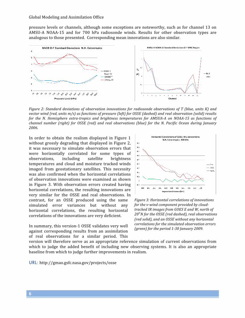
pressure levels or channels, although some exceptions are noteworthy, such as for channel 13 on AMSU-‐A NOAA-‐15 and for 700 hPa radiosonde winds. Results for other observation types are analogous to those presented. Corresponding mean innovations are also similar.
Figure 2: Standard deviations of observation innovations for radiosonde observations of T (blue, units K) and vector wind (red, units m/s) as functions of pressure (left) for OSSE (dashed) and real observation (solid) results for the N. Hemisphere extra-tropics and brightness temperatures for AMSUA-A on NOAA-15 as functions of channel number (right) for OSSE (red) and real observations (blue) for the N. Pacific Ocean during January 2006. In order to obtain the realism displayed in Figure 1 without grossly degrading that displayed in Figure 2, it was necessary to simulate observation errors that were horizontally correlated for some types of observations, including satellite brightness temperatures and cloud and moisture tracked winds imaged from geostationary satellites. This necessity was also confirmed when the horizontal correlations of observation innovations were examined as shown in Figure 3. With observation errors created having horizontal correlations, the resulting innovations are very similar for the OSSE and real observations. In contrast, for an OSSE produced using the same simulated error variances but without any horizontal correlations, the resulting horizontal correlations of the innovations are very deficient. In summary, this version-‐1 OSSE validates very well against corresponding results from an assimilation of real observations for a similar period. This version will therefore serve as an appropriate reference simulation of current observations from which to judge the added benefit of including new observing systems. It is also an appropriate baseline from which to judge further improvements in realism. URL: http://gmao.gsfc.nasa.gov/projects/osse
Figure 3: Horizontal correlations of innovations for the v-wind component provided by cloud-tracked IR images from GOES E and W, north of 20°N for the OSSE (red dashed), real observations (red solid), and an OSSE without any horizontal correlations for the simulated observation errors (green) for the period 1-30 January 2009.

2009 Research Highlights
7
The Simulation of Doppler Wind Lidar Observations in Support of Future Instruments Will McCarty, Ronald Errico, Runhua Yang, Ronald Gelaro Project Goals: The goal of this effort is to address the potential impact of future spaceborne Doppler wind lidar missions on analyses and forecasts produced from the Goddard Earth Observing System (GEOS) data assimilation system by using an Observing System Simulation Experiment (OSSE) framework. Similarly, these experiments are being utilized to develop the system for these new data.
Project Description: To maximize the utility of a future spaceborne instrument in the context of data assimilation, it is best to utilize the heritage of such instruments to prepare the data assimilation as much as possible prior to launch. For instruments that have no predecessor, this approach becomes invalid, as is the case for global Doppler wind lidar measurements. To compensate, observations can be simulated to characterize the anticipated nature of the future missions. Though the true nature of the future observations will likely differ from the simulation, it fosters the necessary development of the framework within the data assimilation system, limiting the amount of effort necessary post-‐launch for maximum utilization. These concepts are being undertaken at the GMAO, as a partner in the Joint Center for Satellite Data Assimilation, to prepare for the launch of the European Space Agency (ESA)’s Atmospheric Dynamic Mission (ADM-‐Aeolus) set for launch in 2012. These efforts will be expanded to perform OSSE studies for the 3D-‐Winds mission proposed in the NRC’s Decadal Survey. Efforts within the GMAO by Ronald Errico and Runhua Yang have focused on the development of the existing global observing system, from conventional observations such as radiosondes to passive spaceborne radiance measurements (i.e. NASA’s Atmospheric Infrared Sounder). These measurements, combined with Doppler wind lidar measurements using an instrument simulator developed at the Royal Netherlands Meteorological Institute (KNMI), create the baseline control (without lidar) and experiment (with lidar) for this OSSE study. Results: Inherent to an OSSE is a nature run, which is a free-‐run climate simulation from which all observations are simulated. From these simulated observations, data assimilation cycling is performed. For the OSSE experiment to be scientifically valid, the nature run must be representative of meteorological truth and fall within a reasonable climatological spread. Since Doppler wind lidar measurements are actively sensed at shortwave, reflective wavelengths, they are very sensitive to clouds and aerosols. Figure 1 shows the distributions of clouds within the nature run for the northern hemisphere winter relative to a climatological distribution generated from three seasons of CloudSat and CALIPSO
Figure 1: The difference in total cloud fraction between the nature run and three years of CloudSat and CALIPSO data for the Dec/Jan/Feb season. Positive (negative) values indicate that the nature run overestimates (underestimates) clouds relative to the observations.
Global Modeling and Assimilation Office
8
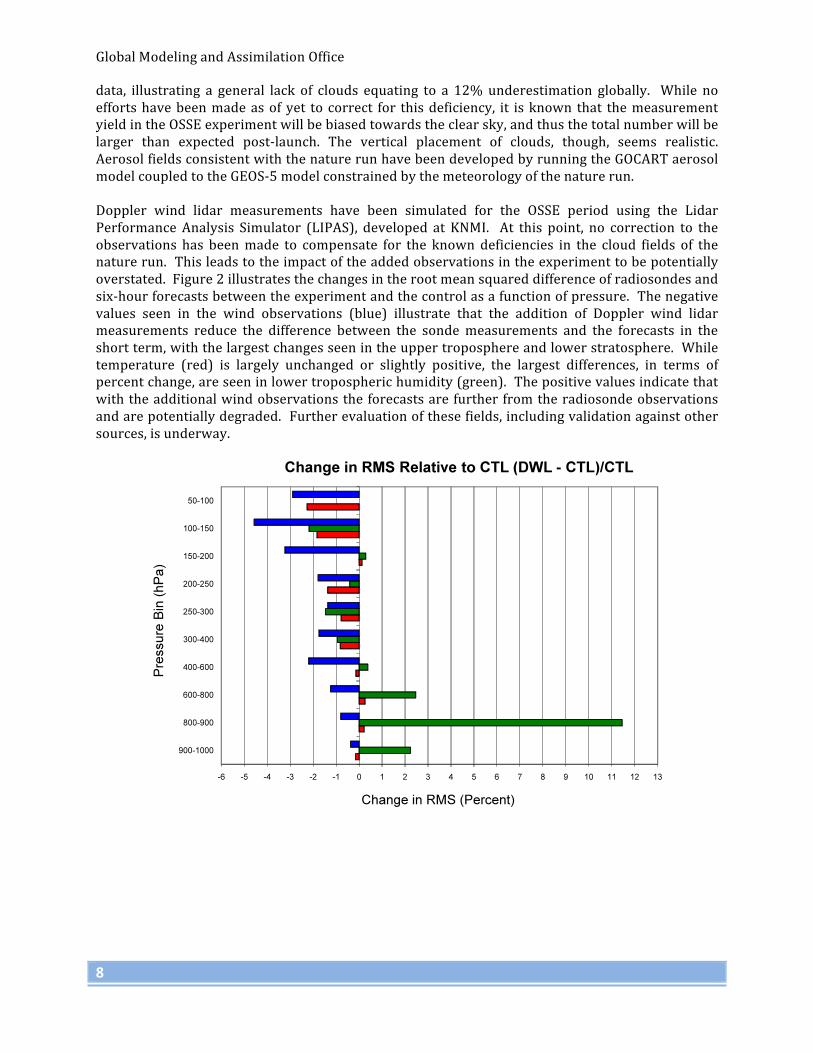
data, illustrating a general lack of clouds equating to a 12% underestimation globally. While no efforts have been made as of yet to correct for this deficiency, it is known that the measurement yield in the OSSE experiment will be biased towards the clear sky, and thus the total number will be larger than expected post-‐launch. The vertical placement of clouds, though, seems realistic. Aerosol fields consistent with the nature run have been developed by running the GOCART aerosol model coupled to the GEOS-‐5 model constrained by the meteorology of the nature run. Doppler wind lidar measurements have been simulated for the OSSE period using the Lidar Performance Analysis Simulator (LIPAS), developed at KNMI. At this point, no correction to the observations has been made to compensate for the known deficiencies in the cloud fields of the nature run. This leads to the impact of the added observations in the experiment to be potentially overstated. Figure 2 illustrates the changes in the root mean squared difference of radiosondes and six-‐hour forecasts between the experiment and the control as a function of pressure. The negative values seen in the wind observations (blue) illustrate that the addition of Doppler wind lidar measurements reduce the difference between the sonde measurements and the forecasts in the short term, with the largest changes seen in the upper troposphere and lower stratosphere. While temperature (red) is largely unchanged or slightly positive, the largest differences, in terms of percent change, are seen in lower tropospheric humidity (green). The positive values indicate that with the additional wind observations the forecasts are further from the radiosonde observations and are potentially degraded. Further evaluation of these fields, including validation against other sources, is underway.
Figure 2: The change in the RMS difference between radiosondes and 6-hr forecasts for wind (blue), temperature (red), and moisture (green) measurements. Negative (positive) values indicate that the RMS is reduced (increased) by the addition of Doppler wind lidar measurements.

2009 Research Highlights
9
Aerosol Data Assimilation in GEOS-‐5 Arlindo da Silva, Ravi Govindaraju Project Goals: The purpose of the Goddard Aerosol Assimilation System (GAAS) is to combine the advances in remote sensing of atmospheric aerosols, aerosol modeling, and data assimilation methodology to produce high spatial and temporal resolution 3D aerosol fields, and to assess the impact of these fields on climate modeling and more generally on atmospheric climate simulations.
Project Description: The GMAO strategy for aerosol data assimilation is focused primarily on NASA EOS instruments, including measurements from MODIS, MISR, OMI and PARASOL. CALIPSO retrievals along with in situ measurements from AERONET and EPA’s AirNOW network are the
main source of validation data. Global, high-‐ resolution (nominally 25km) aerosol forecasts from GEOS-‐5 provide the background for a multi-‐channel 2D aerosol optical depth (AOD) analysis. The generation of analysis increments for the 3D aerosol mixing ratio is based on the concept of Lagrangian Displacement Ensembles, taking into consideration flow-‐dependent aspects of the background error. The innovation-‐based statistical quality control of Dee et al. (1999) is used to trim outliers.
Observation and background AOD error variances and correlation errors are estimated with the maximum-‐likelihood approach of Dee and da Silva (1999). Forecast error bias is explicitly treated using the sequential algorithm of Dee and da Silva (1998). Observation bias correction procedures are based on the work of Lary et al. (2010) and Zang and Reid (2006). All the calculations are performed in terms of a new log-‐transformed AOD variable, a quantity derived to have the Gaussian properties assumed in most of these algorithms. Results: We are currently examining the consistency of the EOS aerosol observation system, and developing the necessary observation bias correction models to ensure the homogeneity of the observing system. A useful diagnostic in this regard is the joint probability density function (PDF) of innovation (observation minus background) and analysis increments (analysis minus background). For a homogeneous observing system, one expects a well-‐defined ellipsis with axis intercepting the origin. Figure 1 shows such a PDF for an experiment where MODIS and MISR observations were analyzed, with PARASOL data used passively (without affecting the analysis). While the MODIS and MISR retrievals are relatively homogeneous over the ocean, PARASOL land retrievals are clearly biased compared to these MODIS/MISR observations and need to be either eliminated or bias corrected prior to assimilation.

Global Modeling and Assimilation Office
10
Figure 1: Joint PDF of O-F and A-F for MODIS/AQUA ocean retrievals (left), and PARASOL land retrievals (right). The effectiveness of the sequential background bias correction scheme can be seen in Figure 2 where the monthly mean observation minus analysis residual is depicted.
References Dee, D., and A. da Silva, 1998: Data assimilation in the presence of forecast bias. Quart. J. Roy.
Meteor. Soc., 124, 269-‐295.
Dee, D., and A. da Silva, 1999: Maximum-‐likelihood estimation of forecast and observation error covariance parameters. Part I: Methodology. Mon. Wea. Rev., 127, 1822-‐1834.
Dee, D. P., L. Rukhovets, R. Todling, A. M. da Silva, and J. W. Larson, 2001: An adaptive buddy check for observational quality control. Quart. J. Roy. Meteor. Soc., 127, 2451-‐71.
Lary, D., L.A. Remer, D. MacNeill, B. Roscoe and S. Paradise, 2009: Machine Learning and Bias Correction of MODIS Aerosol Optical Depth. IEEE Geoscience Rem. Sens. Lett., 6, pp. 694.
Zhang, J. and J. S. Reid, 2006: MODIS aerosol product analysis for data assimilation: assessment of over-‐ocean level 2 aerosol optical thickness retrieval. J. Geophys. Res., 111, doi:10.1029/2005JD006898
Figure 2. Monthly mean (June 2008) residuals based on MODIS/TERRA ocean retrievals: Observation minus analysis (left), and observation minus background (right).
2009 Research Highlights
11
Ocean Data Assimilation into the GEOS-‐5 Coupled Model with GMAO’s ODAS-‐2
Christian Keppenne, Guillaume Vernieres, Michele Rienecker, Jossy Jacob, Robin Kovach Project Goal: The goal of this project is to develop and test the second generation of the GMAO’s ocean data assimilation system (ODAS-‐2), a fully model-‐independent system, implemented within the GEOS-‐5 modeling system under the Earth system Modeling Framework (ESMF). One particular focus in the system validation has been the assimilation of remotely sensed sea surface height observations.
Project Description: Data assimilation refers to the process of using a numerical model to interpolate in space and time between sparse and inexact observations. Under certain reasonable assumptions, the Kalman filter can calculate the optimal weights with which to weigh the estimates of the state of a dynamical system (in our case the climate system) provided on the one hand by the model and on the other by the observations in order to arrive at the optimal state estimate. However, the Kalman filter is prohibitively expensive to implement for present-‐day climate models because it requires the propagation of the model background-‐error covariance matrix. For example, in the current implementation of the GMAO coupled model, the background-‐error covariance matrix of the ocean component alone has close to 1015 elements. Nevertheless, a statistical estimation approach known as the ensemble Kalman filter (EnKF) provides an attractive alternative to the Kalman filter by substituting the time propagation of the background-‐error covariances with a relatively small number of model integrations. The GMAO has pioneered the application of the EnKF to complex numerical models of the ocean circulation. Our second-‐generation system (ODAS-‐2) has greatly improved over ODAS-‐1, the first-‐generation system developed for the Poseidon 4 ocean model (Keppenne et al., 2005). ODAS-‐2 can be used either in ocean only integrations or in coupled model experiments with any ESMF compatible ocean and atmospheric model. The current implementation uses the MOM4 ocean model. When ODAS-‐2 is applied in the context of the GEOS-‐5 coupled atmosphere-‐ocean model, the atmospheric model component is constrained by replaying the GMAO atmospheric analysis. Because the dominant timescales of the atmospheric circulation are much shorter than those of most ocean processes of interest, the replay procedure is approximately equivalent to assimilating ocean and atmospheric observations in the same experiment, while being substantially more economical than fully coupled ocean-‐atmosphere assimilation. The complexity of the numerical models used restricts the number of model copies that can be run concurrently on even the most powerful supercomputers. As a result, the analysis has very few degrees of freedom (as many as the ensemble size) while the numerical model has O(107-‐108) degrees of freedom. ODAS-‐2 addresses problems associated with limited ensemble size by combining error-‐covariance information from four sources: an ensemble of model trajectories, past states (lagged instances) along those model trajectories, a static ensemble of error empirical orthogonal functions and analytically formulated functional covariances. The first three covariance-‐information sources are multivariate (i.e., they can be used to update model variables other than what is being observed such as temperature and salt when sea level height is observed) while the fourth is univariate. In addition ODAS-‐2 also combines the EnKF analysis step with a particle-‐filter pre-‐analysis, resulting in more realistic ocean state estimates than the EnKF alone can provide. Another way to address the degrees-‐of-‐freedom limitation is by localizing the analysis procedure. In doing so, a multitude of low-‐dimensional problems is solved rather than one global high-‐

Global Modeling and Assimilation Office
12
dimensional problem. This approach is commonly used in data assimilation and involves a substantial amount of guesswork in determining the size of the localization regions. ODAS-‐2 introduces a completely adaptive algorithm to optimally calculate the localization parameters involved in the processing of each observation. The adaptive algorithm also produces an objective estimate of the representation error of each observation, thereby eliminating some guesswork. Results: Before the Argo era, relatively few observations of the ocean subsurface were available, hence the accuracy of the ocean state estimates during that period is highly dependent on how well the surface observations, especially remotely-‐sensed sea surface height measurements, can be utilized to infer information about the subsurface. Cross-‐validation against temperature, salinity and current profiles from fixed buoys and other in situ measurement sources shows that the new algorithms used in ODAS-‐2 have resulted in performance breakthroughs over ODAS-‐1 as illustrated in Figure 1. Figure 1 shows the improvements in temperature and salinity estimates in ODAS-‐2 when only sea level height anomalies are assimilated over those from a coupled model run without data assimilation. The improvement is measured by the differences in root mean square difference between the analysis or model estimate and independent (i.e., not assimilated) Argo profiles, integrated vertically through the water column from the surface to 2000m. Warm (cold) colors correspond to areas where the assimilation results in the model field that is closer to (further away from) the Argo temperature or salinity profiles. White areas on the pictures correspond to places where no Argo profiles are available for cross-‐validation.
Figure 1: (a) Relative closeness (relative to a control integration without data assimilation) to independent, not-assimilated Argo temperature profiles (integrated vertically) when sea level height anomalies are assimilated. (b) same as (a) for Argo salinity profiles. (See text). References Keppenne, C.L., M.M. Rienecker, N.P. Kurkowski and D.D. Adamec, 2005: Ensemble Kalman filter
assimilation of altimeter and temperature data with bias correction and application to seasonal prediction, Nonlinear Processes in Geophysics, 12, 491-‐503.
Keppenne, C.L., M.M. Rienecker, J.P. Jacob and R.M. Kovach, 2008: Error covariance modeling in the GMAO ocean ensemble Kalman filter, Mon. Wea. Rev., 136, 2964-‐2982.

2009 Research Highlights
13
Assimilation of Satellite-‐derived Skin Temperature Observations into Land Surface Models
Rolf Reichle, Sujay Kumar (Code 614.3), Sarith Mahanama, Randal Koster, Qing Liu Project Goal: The goal of this project is to investigate the potential for assimilating satellite retrievals of land surface temperature (LST) within the Goddard Earth Observing System (GEOS) land data assimilation system. Such a system will improve the characterization of LST background estimates for the assimilation of atmospheric radiances that are sensitive to the land surface.
Project Description: Land surface conditions are intimately connected with the global climate system and have been associated, through different pathways, with atmospheric predictability. Land surface (or “skin”) temperature (LST) lies at the heart of the surface energy balance and is therefore a key variable in weather and climate models. LST influences the latent and sensible heat fluxes to the atmosphere through which it affects the planetary boundary layer and atmospheric convection. LST also plays an important role in the assimilation of atmospheric remote sensing observations. Because forward radiative transfer modeling for surface-‐sensitive (window) channels requires accurate information about land surface conditions, radiance observations from window channels are typically not assimilated. Accurate LST estimation is therefore critical to improving estimates of the surface water, energy, and radiation balance as well as atmospheric temperature and humidity profiles, which in turn are all critical to improving weather and climate forecast accuracy. In this project we assimilated LST retrievals from the International Satellite Cloud Climatology Project (ISCCP) into the Noah and GEOS-‐5 Catchment (CLSM) land surface models using an ensemble-‐based, off-‐line land data assimilation system. LST is described very differently in the two models. CLSM describes LST as a prognostic variable that assigns a small heat capacity to the top 5 cm layer of the soil and the canopy. By contrast, Noah – used operationally at the National Centers for Environmental Prediction (NCEP) – determines skin temperature diagnostically from the surface energy balance. The different strategies for LST modeling in the two land surface models necessitate different approaches to data assimilation. For GEOS-‐5 development, it is critical to understand how CLSM can be used for LST assimilation and whether there are any advantages or disadvantages between the two LST modeling approaches. Moreover, we pay particular attention to bias between observed and modeled LST. Because satellite and model LST typically exhibit different mean values and variability we have developed customized a priori scaling and dynamic bias estimation approaches for LST assimilation. For each of the two land models, we conducted one open loop (no assimilation) ensemble integration and four different experiments in which ISCCP LST retrievals were assimilated. Two of the four assimilation integrations (per model) were performed with the (unscaled) LST retrievals (“s0”), the other two utilized ISCCP retrievals that were scaled to each model’s LST climatology prior to assimilation (“s1”). In each set of two assimilation integrations, one was done without bias correction (“b0”), and the other used the dynamic bias algorithms (“b8”). For each model, we thus compare four assimilation integrations: “s0b0”, “s0b8”, “s1b0”, and “s1b8”. Performance is measured against 27 months of in situ measurements from the Coordinated Energy and Water Cycle Observations Project at 48 stations.

Global Modeling and Assimilation Office
14
Results: Figure 1 shows that LST estimates from Noah and CLSM without data assimilation (“open loop”) are comparable to each other and superior to ISCCP retrievals. For LST, RMSE values are 4.9 K (CLSM), 5.5 K (Noah), and 7.6 K (ISCCP). Similarly, anomaly correlation coefficients (R) are 0.61 (CLSM), 0.63 (Noah), and 0.52 (ISCCP) (not shown). Obviously, the superior skill of the model LST estimates relative to the skill of the ISCCP retrievals limits the improvements that can be expected from assimilating the ISCCP data. Nevertheless, assimilation of ISCCP retrievals provides modest yet statistically significant improvements (over open loop; as indicated by non-‐overlapping 95% confidence intervals) of up to 0.7 K in RMSE (Figure 1) and 0.05 in anomaly R (not shown). The skill of latent and sensible heat flux estimates from the assimilation integrations is essentially identical to the corresponding open loop skill. Noah assimilation estimates of ground heat flux, however, can be significantly worse than open loop estimates (not shown). Provided the assimilation system is properly adapted to each land model, the benefits from the assimilation of LST retrievals are comparable for both models. The main conclusions from the experiments are as follows: (1) There are strong biases between LST estimates from in situ observations, land modeling, and satellite retrievals that vary with season and time-‐of-‐day. Biases of a few Kelvin are typical, with larger values exceeding 10 K. (2) The skill of LST estimates from the CLSM and Noah land model integrations is superior to that of the ISCCP satellite retrievals. (3) Assimilation of ISCCP LST retrievals into the land surface models can improve LST estimates by up to 0.7 K for RMSE and by up to 0.05 for anomaly R, while not making surface turbulent fluxes worse. (4) Gross errors in surface flux estimates can result if biases are not taken into account properly, with a combination of a priori scaling and dynamic bias estimation methods yielding the best overall results. (5) Assimilation diagnostics for integrations without a priori scaling strongly reflect the underlying biases, indicating that without a priori scaling the assimilation system is far from operating in accordance with its underlying assumptions. (6) Provided the assimilation system is properly configured for each land model, the benefits from the assimilation of LST retrievals are comparable for both land models. Publication Reichle, R., S. Kumar, S. Mahanama, R. Koster, and Q. Liu, 2010: Assimilation of satellite-‐derived skin
temperature observations into land surface models, J. Hydrometeorol. (in press).
Figure 1: RMSE versus CEOP in situ observations for LST from ISCCP retrievals, model integrations, and select assimilation integrations without a priori scaling and (b0) without and (b8) with dynamic bias correction.

2009 Research Highlights
15
Toward Energetic Consistency in Data Assimilation
Stephen Cohn Project Goal: The goal of this project is to develop a general, systematic approach to overcome the large, spurious loss of variance that different research groups have found to limit the potential of advanced data assimilation schemes for the atmosphere and ocean. The immediate objective, as the GMAO moves toward development of a long-‐window 4D-‐Var atmospheric data assimilation system, is to take initial steps toward the development of such an approach for this system.
Project Description: Ménard et al. (2000) and Ménard and Chang (2000) noted the problem of spurious loss of variance in a full-‐rank Kalman filter implemented for stratospheric constituent data assimilation on isentropic surfaces. This loss of variance, more than 50% of the correct value throughout the surf zone, could be recognized clearly in that application on the basis of consistency with mass conservation. It was attributed to a magnification of the slight numerical dissipation of the dynamical model by several orders of magnitude, through a shearing mechanism, in the Kalman filter covariance evolution. The problem was addressed by evolving the estimation error variance directly, rather than through the Kalman filter, an approach that is available for constituent transport because transport dynamics imply not only a covariance evolution equation, but a closed variance evolution equation as well. Other well-‐known but ad hoc methods for boosting variance, including “covariance inflation” and the introduction of an artificially large “model error” covariance term, yielded assimilation results inferior even to those obtained through a simple optimal interpolation scheme, while direct evolution of the variance field gave superior results. Experience gained by different research groups in the implementation of ensemble Kalman filters (EnKF) for full-‐blown atmospheric and oceanic data assimilation has revealed that spurious loss of variance is a serious problem also in these applications. For example, Houtekamer and Mitchell (2005) found the unexplained loss of variance in their EnKF implementation for atmospheric data assimilation to be so large that, when measured in a linearized energy norm, it is comparable to the error that would be incurred by neglecting model “physics” entirely. The complexity of full-‐blown atmospheric data assimilation relative to offline constituent data assimilation makes it much more difficult to sort out the root cause or causes of spurious variance loss, and therefore to address the problem systematically. Houtekamer and Mitchell (2005) have suggested referring to the artificially large model error term they found necessary to counter the spurious variance loss as a “system error” term instead, to acknowledge the fact that the true source or sources of variance loss remain unclear. What is by now widely understood is that spurious variance loss leads to “ensemble collapse” and therefore to filter divergence if left untreated, but that current approaches to the problem are ad hoc and cannot fully address it. The GMAO is now beginning development of a long-‐window, weak-‐constraint version of its 4D-‐Var atmospheric data assimilation system. The new version will allow for inclusion of a model error term, completely absent in the current strong-‐constraint version that in principle should allow the assimilation window to be lengthened. Because of the rough theoretical equivalence between long-‐window, weak-‐constraint 4D-‐Var and Kalman filtering, the research experience sketched above suggests that addressing the problem of spurious variance loss in this new context will be important for realizing the potential benefit of the 4D-‐Var system. Moreover, addressing the problem is expected to be more difficult in the 4D-‐Var context than in that of (ensemble) filtering, primarily because the highly implicit nature of the covariance evolution in 4D-‐Var does not yield an

Global Modeling and Assimilation Office
16
internal measure of perceived variance. The project has therefore begun with an investigation of the problem of variance loss to determine its root cause and how it might be addressed in general, rather than for any particular data assimilation algorithm. Results: Initial results of the investigation are reported in Cohn (2010, hereafter C10). The principle of energetic consistency (PEC) was established in C10 and used there to examine many of the probabilistic assumptions and computational approximations commonly employed in data assimilation. The PEC is a general relationship that holds between the first two moments of a stochastic system, which are the total energy of the mean state and the total variance of the state estimate when the state variables are chosen to be energy variables for the system. It provides a powerful tool for diagnosing and understanding many of the difficulties of data assimilation, due to its broad applicability. It was shown in C10 that of the major assumptions and approximations used in data assimilation, it is primarily the use of even a slightly dissipative numerical model that can, and in typical circumstances must, result in a large, spurious loss of variance and consequent filter divergence. The PEC was used also in C10 to show that a general, direct way to address the problem is to incorporate an appropriate anti-‐dissipative operator in the covariance evolution. In the EnKF context this can be done on the ensemble covariance operator and in the 4D-‐Var context it can be accomplished by modifying the tangent linear operator. This approach can be thought of as a generalization of ad hoc ``covariance inflation,'' to selectively and immediately amplify only those scales whose energy is being dissipated, rather than amplifying all scales equally. The approach appears to be implementable with the development of the GMAO weak-‐constraint 4D-‐Var system, and on the basis of experimental and theoretical results obtained so far, appears promising as one of many contributions that will be necessary to obtain real improvement over strong-‐constraint 4D-‐Var. Steps toward implementing this approach planned for the coming year include development of a way to measure perceived variance in the 4D-‐Var system, to allow for diagnosis of variance loss in the system, and the preliminary formulation of an anti-‐dissipative operator appropriate for use with the finite-‐volume dynamical core. References Cohn, S. E., 2010: The principle of energetic consistency in data assimilation. In Data Assimilation:
Making Sense of Observations, W. Lahoz, B. Khattatov and R. Ménard (eds.), Ch. 7, pp. 137–216, Springer (in press).
Houtekamer, P. L., and H. L. Mitchell, 2005: Ensemble Kalman filtering. Quart. J. Roy. Meteor. Soc., 131, 3269–3289.
Ménard, R., and L. P. Chang, 2000: Assimilation of stratospheric chemical tracer observations using a Kalman filter. Part II: χ2-‐validated results and analysis of variance and correlation dynamics. Mon. Wea. Rev., 128, 2672–2686.
Ménard, R., and Co-‐authors, 2000: Assimilation of stratospheric chemical tracer observations using a Kalman filter. Part I: Formulation. Mon. Wea. Rev., 128, 2654–2671.
2009 Research Highlights
17
Improved Simulation of Tropical Organization in GEOS-‐5
Andrea Molod, Julio Bacmeister (NCAR), Max Suarez Project Goal: GEOS-‐5 developments are driven by the need to have a comprehensive global model valid for both weather and climate and for use in both simulation and assimilation. The goal of this project is to improve the subgridscale parameterizations that impact the model performance for all of these applications, with special focus on model performance in the tropics.
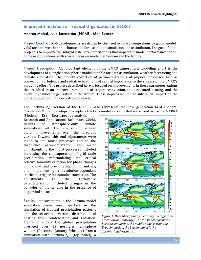
Project Description: An important element of the GMAO atmospheric modeling effort is the development of a single atmospheric model suitable for data assimilation, weather forecasting and climate simulation. The model’s collection of parameterizations of physical processes such as convection, turbulence and radiative heating is of central importance to the success of the GMAO’s modeling effort. The project described here is focused on improvements in these parameterizations that resulted in an improved simulation of tropical convection, the associated heating, and the overall dynamical organization in the tropics. These improvements had substantial impact on the model simulation in the extratropics as well. The Fortuna 2_0 version of the GEOS-‐5 GCM represents the new generation GCM (General Circulation Model) developed to replace the Eros model versions that were used as part of MERRA (Modern Era Retrospective-‐analysis for Research and Applications, Bosilovich, 2008). Results of atmosphere-‐only climate simulations with the new version exhibit major improvements over the previous version. Towards this end adjustments were made to the moist processes and to the turbulence parameterization. The major adjustments to the moist processes included increasing the re-‐evaporation of grid scale precipitation, reformulating the critical relative humidity criterion for phase changes of in-‐cloud and precipitating liquid and ice, and implementing a resolution-‐dependant stochastic trigger for cumulus convection. The adjustments to the turbulence parameterization included changes in the behavior of the scheme in the presence of large wind shear. Results: Improvements in the Fortuna model simulation were most marked in the simulation of tropical precipitation patterns and the associated vertical distribution of heating from condensation and radiation. Figure 1 shows the global precipitation averaged over 15 northern hemisphere winters (December-‐January-‐February) from a simulation with Fortuna-‐2_0 (top panel), a
Figure 1: December-January-February average total precipitation (mm/day). The top panel is from the Fortuna simulation, the middle panel is from the Eros simulation, the bottom panel is the observational estimate.

Global Modeling and Assimilation Office
18
simulation with an Eros version (middle panel), and from the merged in situ and satellite-‐based estimate of precipitation from GPCP (Global Precipitation Climatology Project). The Fortuna-‐2_0 simulation shows improvements relative to GPCP over land areas in southern Africa, South America and northern Australia. Improvements in precipitation patterns are also marked over two important ocean regions, one near Indonesia, where the Fortuna precipitation occurs nearer the correct latitude, the other in the extension of the precipitation region southward and eastward across the Pacific in the southern hemisphere. Many studies (e.g., Wallace and Gutzler, 1981) have shown that the pattern of tropical precipitation is associated with the excitation and propagation into the extratropics of large scale and steady wave patterns, seen as a series of ridges and troughs starting in the north Pacific and extending across the North American continent. These ‘teleconnections’ translate the improved tropical precipitation pattern in the Fortuna simulation into improvements in the model simulation of ‘stationary waves’. An indicator of the stationary wave pattern is the deviation from the zonal mean geopotential height field (eddy height), shown in Figure 2 at the 300 hPa level. Again, as in Figure 1, the top panel shows the Fortuna model result, the middle panel the Eros model result, and the bottom panel the result from MERRA. The differences as measured against MERRA between the Fortuna and Eros simulation of the ridge and trough pattern over North America show the improved stationary wave pattern. Model simulations with Fortuna-‐2_0 showed bias in the cloud cover field and in the associated surface radiation fields which necessitated some changes in the cloud and condensation algorithms. These algorithm changes were included in Fortuna-‐2_1, currently being used to perform ocean-‐atmosphere coupled simulations in the GMAO. The condensation and cloud-‐radiation interaction elements of the model remain the focus of current development efforts. References Bosilovich, M., 2008: NASA’s Modern Era Retrospective-‐analysis for Research and Applications:
Integrating Earth Observations. Earthzine September 2008 Articles, Climate, Earth Observation (http://www.earthzine.org/2008/09/26/nasas-‐modern-‐era-‐retrospective-‐analysis/)
Wallace, J.M. and D.S. Gutzler, 1981: Teleconnections in the geopotential height field during the Northern Hemisphere winter. Mon. Wea. Rev., 109, 785-‐812.
Figure 2: December-January-February average eddy height at 300 hPa (m). Top panel is from the Fortuna simulation, middle panel is from the Eros simulation, and bottom panel is the observational estimate.
2009 Research Highlights
19
The GEOS-‐5 Coupled Atmosphere-‐Ocean Model
Yury Vikhliaev, Max Suarez, Andrea Molod, Bin Zhao, Michele Rienecker Project Goal: The goal of this work is development of a GEOS-‐5 coupled atmosphere-‐ocean general circulation model (AOGCM) for short-‐term climate prediction.
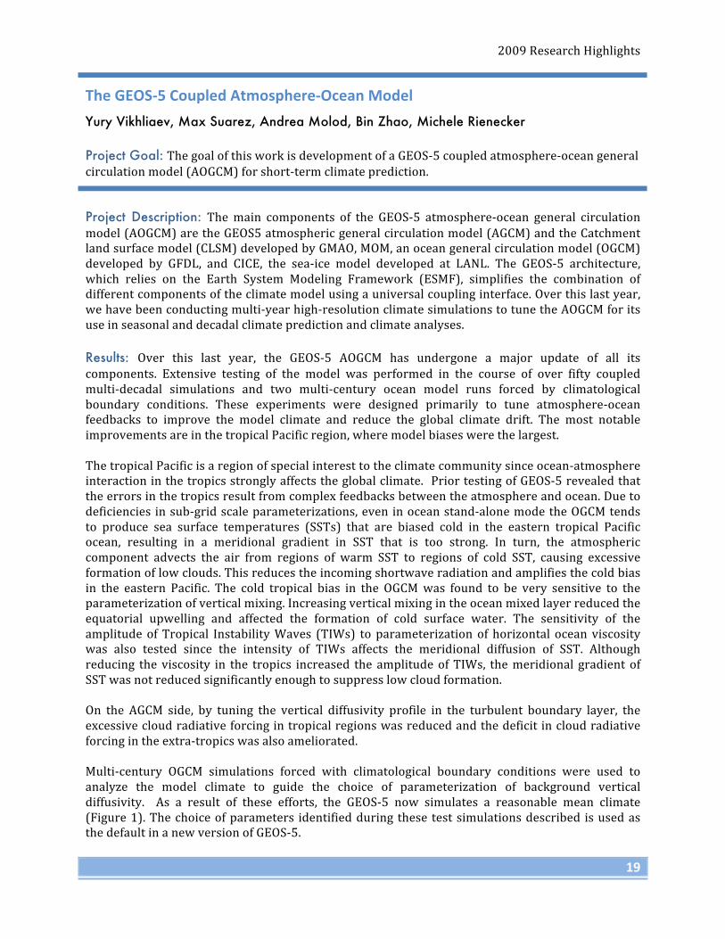
Project Description: The main components of the GEOS-‐5 atmosphere-‐ocean general circulation model (AOGCM) are the GEOS5 atmospheric general circulation model (AGCM) and the Catchment land surface model (CLSM) developed by GMAO, MOM, an ocean general circulation model (OGCM) developed by GFDL, and CICE, the sea-‐ice model developed at LANL. The GEOS-‐5 architecture, which relies on the Earth System Modeling Framework (ESMF), simplifies the combination of different components of the climate model using a universal coupling interface. Over this last year, we have been conducting multi-‐year high-‐resolution climate simulations to tune the AOGCM for its use in seasonal and decadal climate prediction and climate analyses. Results: Over this last year, the GEOS-‐5 AOGCM has undergone a major update of all its components. Extensive testing of the model was performed in the course of over fifty coupled multi-‐decadal simulations and two multi-‐century ocean model runs forced by climatological boundary conditions. These experiments were designed primarily to tune atmosphere-‐ocean feedbacks to improve the model climate and reduce the global climate drift. The most notable improvements are in the tropical Pacific region, where model biases were the largest. The tropical Pacific is a region of special interest to the climate community since ocean-‐atmosphere interaction in the tropics strongly affects the global climate. Prior testing of GEOS-‐5 revealed that the errors in the tropics result from complex feedbacks between the atmosphere and ocean. Due to deficiencies in sub-‐grid scale parameterizations, even in ocean stand-‐alone mode the OGCM tends to produce sea surface temperatures (SSTs) that are biased cold in the eastern tropical Pacific ocean, resulting in a meridional gradient in SST that is too strong. In turn, the atmospheric component advects the air from regions of warm SST to regions of cold SST, causing excessive formation of low clouds. This reduces the incoming shortwave radiation and amplifies the cold bias in the eastern Pacific. The cold tropical bias in the OGCM was found to be very sensitive to the parameterization of vertical mixing. Increasing vertical mixing in the ocean mixed layer reduced the equatorial upwelling and affected the formation of cold surface water. The sensitivity of the amplitude of Tropical Instability Waves (TIWs) to parameterization of horizontal ocean viscosity was also tested since the intensity of TIWs affects the meridional diffusion of SST. Although reducing the viscosity in the tropics increased the amplitude of TIWs, the meridional gradient of SST was not reduced significantly enough to suppress low cloud formation. On the AGCM side, by tuning the vertical diffusivity profile in the turbulent boundary layer, the excessive cloud radiative forcing in tropical regions was reduced and the deficit in cloud radiative forcing in the extra-‐tropics was also ameliorated. Multi-‐century OGCM simulations forced with climatological boundary conditions were used to analyze the model climate to guide the choice of parameterization of background vertical diffusivity. As a result of these efforts, the GEOS-‐5 now simulates a reasonable mean climate (Figure 1). The choice of parameters identified during these test simulations described is used as the default in a new version of GEOS-‐5.
Global Modeling and Assimilation Office
20
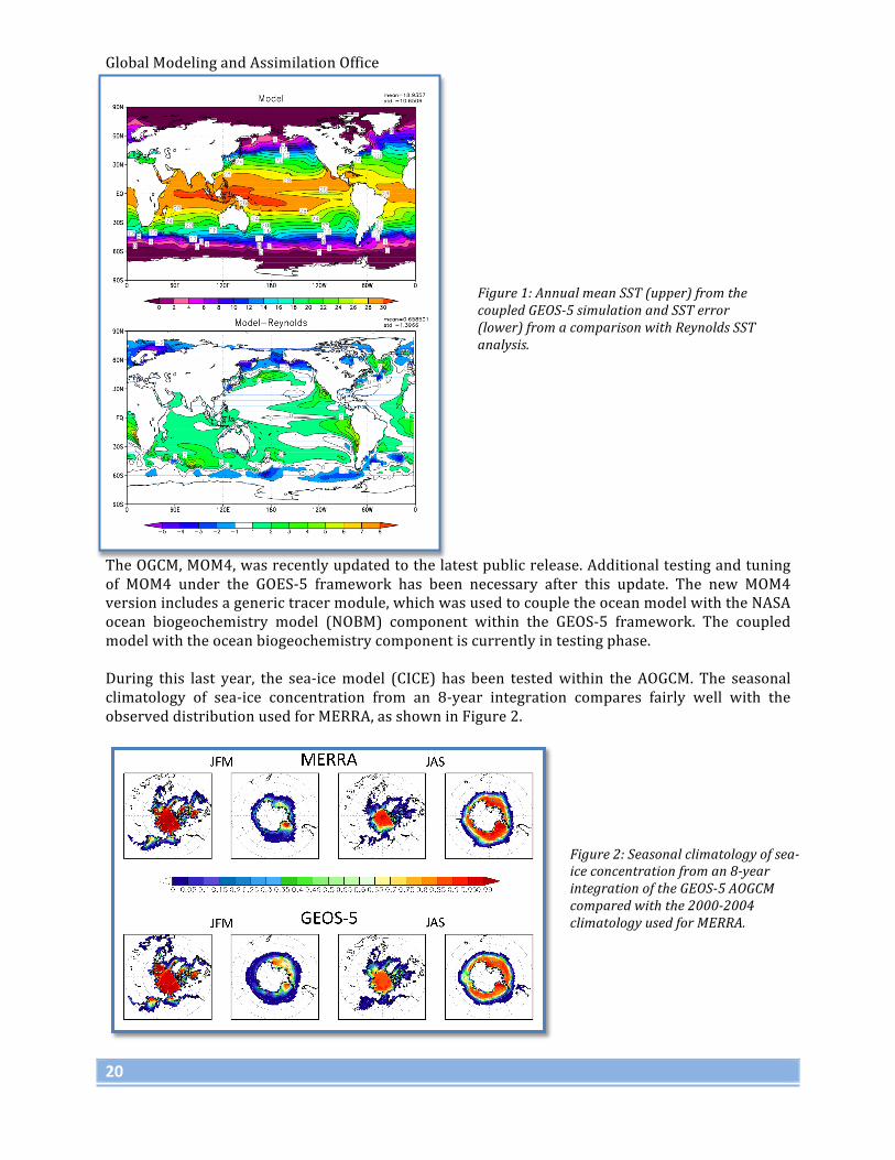
The OGCM, MOM4, was recently updated to the latest public release. Additional testing and tuning of MOM4 under the GOES-‐5 framework has been necessary after this update. The new MOM4 version includes a generic tracer module, which was used to couple the ocean model with the NASA ocean biogeochemistry model (NOBM) component within the GEOS-‐5 framework. The coupled model with the ocean biogeochemistry component is currently in testing phase. During this last year, the sea-‐ice model (CICE) has been tested within the AOGCM. The seasonal climatology of sea-‐ice concentration from an 8-‐year integration compares fairly well with the observed distribution used for MERRA, as shown in Figure 2.
Figure 1: Annual mean SST (upper) from the coupled GEOS-5 simulation and SST error (lower) from a comparison with Reynolds SST analysis.
Figure 2: Seasonal climatology of sea-ice concentration from an 8-year integration of the GEOS-5 AOGCM compared with the 2000-2004 climatology used for MERRA.
2009 Research Highlights
21
Cloud Parameterization using CRM Simulations and Satellite Data
Peter Norris, Arlindo da Silva, Lazaros Oreopoulos (code 613.2) Project Goals: The essential role that clouds play in moderating climate has prompted continuing efforts to improve the representation of clouds in global climate models. What is currently needed is the ability to test these cloud representations against observed cloud data with global or large-‐scale coverage such as from NASA’s high-‐resolution satellite cloud observing systems (e.g., MODIS, AMSR-‐E and CloudSat). The goal of our work is to use retrieved cloud data to validate cloud properties within the Goddard Earth Observing System (GEOS) model, to measure the capability of trial cloud representations, and to assimilate cloud measurements directly into the GEOS data assimilation system. The project is particularly concerned with developing climate model cloud representations that benefit from realistic statistical descriptions of the cloud scale variability provided by high-‐resolution NASA cloud data.
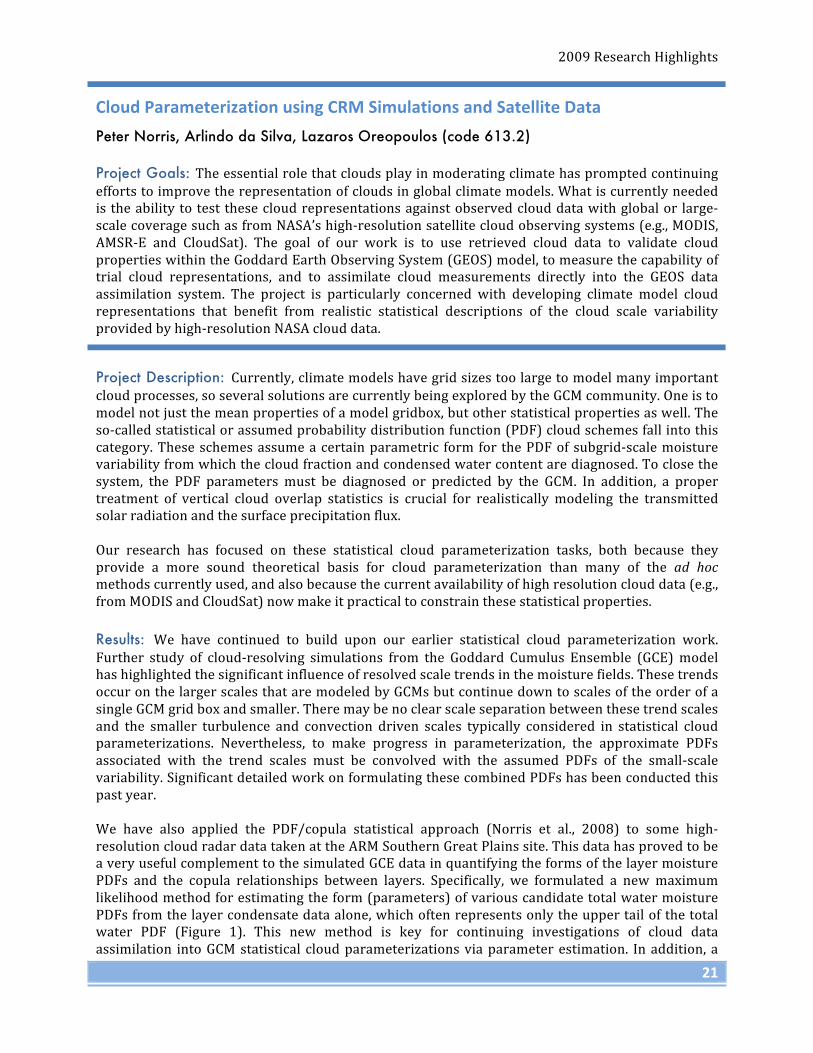
Project Description: Currently, climate models have grid sizes too large to model many important cloud processes, so several solutions are currently being explored by the GCM community. One is to model not just the mean properties of a model gridbox, but other statistical properties as well. The so-‐called statistical or assumed probability distribution function (PDF) cloud schemes fall into this category. These schemes assume a certain parametric form for the PDF of subgrid-‐scale moisture variability from which the cloud fraction and condensed water content are diagnosed. To close the system, the PDF parameters must be diagnosed or predicted by the GCM. In addition, a proper treatment of vertical cloud overlap statistics is crucial for realistically modeling the transmitted solar radiation and the surface precipitation flux. Our research has focused on these statistical cloud parameterization tasks, both because they provide a more sound theoretical basis for cloud parameterization than many of the ad hoc methods currently used, and also because the current availability of high resolution cloud data (e.g., from MODIS and CloudSat) now make it practical to constrain these statistical properties. Results: We have continued to build upon our earlier statistical cloud parameterization work. Further study of cloud-‐resolving simulations from the Goddard Cumulus Ensemble (GCE) model has highlighted the significant influence of resolved scale trends in the moisture fields. These trends occur on the larger scales that are modeled by GCMs but continue down to scales of the order of a single GCM grid box and smaller. There may be no clear scale separation between these trend scales and the smaller turbulence and convection driven scales typically considered in statistical cloud parameterizations. Nevertheless, to make progress in parameterization, the approximate PDFs associated with the trend scales must be convolved with the assumed PDFs of the small-‐scale variability. Significant detailed work on formulating these combined PDFs has been conducted this past year. We have also applied the PDF/copula statistical approach (Norris et al., 2008) to some high-‐resolution cloud radar data taken at the ARM Southern Great Plains site. This data has proved to be a very useful complement to the simulated GCE data in quantifying the forms of the layer moisture PDFs and the copula relationships between layers. Specifically, we formulated a new maximum likelihood method for estimating the form (parameters) of various candidate total water moisture PDFs from the layer condensate data alone, which often represents only the upper tail of the total water PDF (Figure 1). This new method is key for continuing investigations of cloud data assimilation into GCM statistical cloud parameterizations via parameter estimation. In addition, a
Global Modeling and Assimilation Office
22
related method was developed to constrain the inter-‐layer rank correlations of total moisture using the condensate data from pairs of separated layers. These inter-‐layer correlations are needed to parameterize GCM cloud overlap and cloudy radiative transfer. The above two works – on a general and flexible parameteric form for subgrid-‐scale moisture variability and on the estimation of the parameters of that variability using ARM condensate data – tie in very well to the larger goal of cloud data assimilation into GEOS-‐5. For assimilation, we have been working on appropriate methods to handle cloud observations from MODIS and other instruments in the context of multiple cloud layers within a GCM grid box sized domain.
Publication Liu, H., J. H. Crawford, D. B. Considine, S. Platnick, P. M. Norris, B. N. Duncan, R. B. Pierce, G. Chen,
and R. M. Yantosca, 2009: Sensitivity of photolysis frequencies and key tropospheric oxidants in a global model to cloud vertical distributions and optical properties. J. Geophys. Res., 114, D10305, doi:10.1029/2008JD011503.
Reference Norris, PM, L. Oreopoulos, A.Y. Hou, W.-‐K. Tao, X. Zeng, 2008. Representation of 3D heterogeneous
cloud fields using copulas: Theory for water clouds. Quart. J. Roy. Meteorol. Soc., 134, 1843-‐1864. doi:10.1002/qj.321.
Figure 1: “Tail-fitted” total moisture PDFs from Cloud Resolving Model output. These fits use only the saturated data to the right of the dashed line, plus the number only (not the values) of sub-saturated data points. Even a 10% cloud fraction is often sufficient for a good fit! This shows the promise in estimating PDF parameters from high-resolution satellite cloud observations of partially cloudy scenes.

2009 Research Highlights
23
The Impact of Altimetry and Argo data on GMAO’s Seasonal Forecasts
Michele Rienecker, Robin Kovach, Christian Keppenne, Jelena Marshak Project Goals: The goal of the seasonal prediction efforts in the GMAO is to improve forecast skill using satellite observations. For the ocean, the focus has been on satellite altimetry, available since 1993.
Project Description: Ocean assimilation systems synthesize diverse in situ and satellite data streams into four-‐dimensional state estimates by combining the various observations with the model states. Assimilation is particularly important for the ocean where subsurface observations, even today, are sparse and intermittent compared with the scales needed to represent ocean variability and where satellites only sense the surface. Since the ocean is the source of long-‐term memory in the climate system, a critical element in climate forecasting with coupled models is the initialization of the ocean with states from a data assimilation system.
The current GMAO seasonal forecasting system is based on the NSIPP coupled model, CGCMv1, and the ocean is initialized from offline assimilation using our ocean data assimilation system, version1 (ODAS-‐1). The ocean model is the Poseidon ocean model, version 4. ODAS-‐1 allows both univariate and multivariate assimilation implementations. For global data assimilation, the multivariate system is the Ensemble Kalman Filter (EnKF). It provides a prognostic calculation of the state-‐dependent forecast error covariances, including the statistics needed to project the information from the surface altimeter data to the interior ocean. Since sea surface height anomalies are assimilated, we use the online bias estimation procedure of ODAS-‐1 to estimate the offset between the data and the model forecast.
Ocean assimilation experiments were conducted as ocean-‐only runs forced with daily surface wind stress derived from SSM/I and QuikSCAT, GPCP monthly mean precipitation, NCEP CDAS1 shortwave radiation (for penetrating radiation) and latent heat flux (for evaporation). Surface heat fluxes are provided by relaxation to weekly SST analyses. A relaxation to sea surface salinity climatology is used to compensate for biases in the freshwater flux and the omission of river runoff. The TAO mooring array in the equatorial Pacific provides the backbone of the ocean observing system to support seasonal prediction. The altimeter data, available from October 2002, provide data where very little in situ data are available, especially the equatorial Indian and Atlantic Oceans. The global ocean observing system underwent a significant upgrade with the availability of Argo drifters, beginning in 2001. The drifter array was fairly complete by 2004. The impact of the ocean analyses on oceanic seasonal forecast skill – both SST and thermocline variability (estimated by the average temperature in the upper 300 m) – in the GMAO coupled model forecasts have been assessed for the ocean initialized with all data assimilated (1993-‐2008), with SSH withheld (1993-‐2008) and with Argo withheld (2001-‐2008).
Results: We compare the skill of forecasts initialized in January, March, July, and October. Each forecast experiment comprises 8 ensemble members. In each case, the atmosphere was initialized from the appropriate NCEP analysis. The skill for upper-‐ocean temperature and SST in the tropical oceans is summarized in Figure 1 where the fields are averaged over the regions shown in Figure 2.

Global Modeling and Assimilation Office
24
Figure 1: The impact of altimetry and Argo data on forecast skill for different regions, as measured by the reduction in mean absolute error for the forecast range 1-3 months (left-hand columns) and 4-6 months (right-hand columns). The upper plots are for average temperature in the upper 300m, the lower for SST. The impact of SSH assimilation is shown for both the entire period (1993-2008) and also for the Argo era (2001-2008) for comparison. Only impacts that are significant at the 70% level are shown.
A positive impact from altimetry is found in the central equatorial Pacific (NINO3) and the North Subtropical Atlantic (NSTRATL), although the impact in the Pacific often does not last through the second season. Interestingly, Argo has a much stronger impact on SST than on the subsurface temperature, except in the Indian Ocean. In the Indian Ocean the impacts from both observation types are positive in the second
season, with the impact from altimetry slightly stronger than that from Argo, except in the subsurface SETIO. The impacts from Argo on the Atlantic SST are opposite from those for subsurface temperature in the second season. The differences between the impacts of SSH for 2001-‐2008 and for 1993-‐2008 indicate not only the changes in predictability for different periods, but also that we need a longer time series for robust results. Unfortunately, the changing observing system makes this problematic. Publication Rienecker, M.M., R. Kovach, C.L. Keppenne, and J. Marshak, 2010: NASA’s Ocean Observations for
Climate Analysis and Prediction. Bull. Am. Meteorol. Soc. (submitted to special collection for NASA’s Earth Sciences at 20).
Figure 2: The regions used to assess the mean absolute forecast error shown in Figure 1.

2009 Research Highlights
25
Snow and Soil Moisture Contributions to Seasonal Streamflow Prediction Randy Koster, Sarith Mahanama, Ben Livneh (U. Washington), Dennis Lettenmaier (U. Washington), Rolf Reichle Project Goal: The analysis aims to quantify, using a suite of state-‐of-‐the-‐art land surface models (LSMs), the relative contributions of snow information and soil moisture information to the accurate forecasting of streamflow at seasonal leads.
Project Description: Improved seasonal streamflow predictions have obvious benefits, helping water resource managers, for example, optimize reservoir operations and mitigate the destructive capacity of floods and droughts. Several climate mechanisms are potential contributors to skill in streamflow prediction. Western water managers rely heavily on snow observations to project post-‐snow-‐season water availability. A second potential contributor is the accurate forecasting of post-‐winter meteorological anomalies (precipitation and temperature) from wintertime climate conditions, particularly ocean temperatures. A third is knowledge of wintertime soil moisture contents below the snowpack: if the soil is dry below the snowpack, more of the spring snowmelt water may infiltrate the soil and later evaporate, whereas a wet soil below the snowpack may encourage greater streamflow and a more efficient filling of reservoirs. Here we quantify seasonal forecast skill associated with snow and soil moisture initialization using (i) multi-‐decadal naturalized streamflow measurements covering much of the western United States, (ii) a suite of state-‐of-‐the-‐art land surface modeling systems (the GMAO catchment, VIC, Noah, and Sacramento LSMs), and (iii) true forecast experiments. The four models were integrated over the period 1920-‐2003 on a 0.5° grid covering CONUS using an hourly, observations-‐based, surface meteorological forcing data set. This 84-‐year simulation, labeled CTRL, provides a “maximum possible model performance” for comparison with our forecast experiments. Three prediction experiments (Exp1, Exp2, and Exp3) were then performed with each LSM, experiments designed to quantify the degree to which March-‐July (MAMJJ) streamflow can be predicted from January 1 conditions assuming no skill in the seasonal prediction of meteorological forcing. Exp1 consists of 84 separate 7-‐month forecasts (one for each year of 1920-‐2003) initialized on January 1 with the January 1 snowpack and soil moisture states produced by CTRL for the year in question. To represent a lack of knowledge of meteorological forcing during the forecast period, the LSM was integrated with the climatological seasonal cycle of diurnal forcing determined from the CTRL forcing files; thus, any skill generated in the forecast MAMJJ streamflows is attributable to the initialization alone. Exp2 is identical to Exp1, except that soil moisture was initialized with the climatological distribution of January 1 soil moisture; thus, in Exp2, no forecast skill was derived from soil moisture information – Exp2 relied solely on snow initialization for skill. Analogously, Exp3 is identical to Exp1, except that snow amounts were initialized to the climatological January 1 fields; thus, Exp3 relied solely on soil moisture initialization for forecast skill. Results: Figure 1 shows the outlines of the 17 basins examined. For each experiment, the MAMJJ streamflows produced by each model were averaged across the grid cells within a basin and then combined into a single multi-‐model basin average. The average forecasts were evaluated against naturalized streamflow gauge data for the basin. CTRL represents the best possible model simulation of observed streamflow because it makes use of both observations-‐based initial conditions and observations-‐based post-‐winter meteorological forcing. (CTRL thus does not consist of true forecasts.) Agreement between the CTRL results and

Global Modeling and Assimilation Office
26
the streamflow observations during the periods of overlap is presented in the top left panel of Figure 1. Agreement, or skill, is measured here in terms of the square of the correlation coefficient (r2) between the observed time series of MAMJJ streamflows and the corresponding multi-‐model average time series. The r2 values for CTRL vary from about 0.3 to 0.9, so while CTRL does capture 30-‐90% of the observed streamflow variance, this “best” simulation is not perfect, presumably due to deficiencies in the forcing and validation data and in the models. The top right panel of Figure 1 shows the prediction skill obtained in Exp1, i.e., that obtained from knowing only the January 1 initial conditions. The r2 values are reasonably large (up to ~ 0.5) and are generally significant at the 95% level. Thus, we see our first important result: the uncalibrated models predict, with some skill, observed streamflow months in advance without knowledge
(beyond climatology) of meteorological conditions The two bottom panels in Figure 1 show the skill metrics for Exp2 and Exp3. They show the isolated contributions of snow and soil moisture initializations to the streamflow forecast skill. Here we see our second important result: snow initialization is the dominant contributor to skill in most basins, particularly in the mountainous areas toward the northwest, whereas soil moisture initialization contributes significantly to skill in many basins, particularly toward the southeast (e.g., at gauges along the Colorado and Arkansas Rivers). In some of the southeastern basins, soil moisture contributes more to skill than snow does. Figure 1 demonstrates that the initialization of snow and soil moisture on January 1
contributes skill to forecasts of MAMJJ streamflow across a broad sampling of western U.S. basins. Today’s state-‐of-‐the-‐art land surface models, without calibration, are thus at a level of maturity suitable for transforming soil moisture and snowpack information into skillful streamflow forecasts. The study speaks to the potential value of improved snow and soil moisture observations, e.g., through space-‐based sensors (GPM, SMAP).
Publication Koster, R. D., S. P. P. Mahanama, B. Livneh, D. Lettenmaier, and R. Reichle, 2010: Land surface
modeling systems can produce skillful forecasts at seasonal leads. Nature Geoscience (submitted).
Figure 1: Streamflow skill levels, plotted by basin. a. CTRL, b. Exp1 forecasts (skill derived solely from knowledge of January 1 soil moisture (SM) and snow conditions), c. Exp2 forecasts, and d. Exp3 forecasts. Gray coloring indicates that a skill level is not significantly different from zero at the 95% confidence level.

2009 Research Highlights
27
Skill Assessment of a Spectral Ocean-‐Atmosphere Radiative Model
Watson Gregg, Nancy Casey Project Goals: The project goal is to develop accurate and efficient radiative transfer for the atmosphere and oceans at sufficient spectral resolution to support ocean ecology, photosynthesis, biogeochemistry, and heat exchange investigations, and of sufficient duration to support inter-‐annual and decadal investigations.
Project Description: When light enters the ocean from the atmosphere, it initiates a series of events that leads to the existence of nearly all marine life. The first event in this sequence is photosynthesis, where ocean phytoplankton absorb light and convert it to organic carbon. Light, or irradiance, entering the ocean is thus critical for marine photosynthesis, ecosystems, fisheries, and carbon dynamics. Additionally, the irradiance absorbed by the ocean plays a critical role in the temperature of the ocean, contributes to the vertical density structure and surface ocean photochemistry, and affects the exchange of heat with the atmosphere. Models and algorithms simulating these processes require realistic representations of irradiance entering the oceans. This begins with irradiance propagation through the atmosphere and into the ocean surface. There are many radiative transfer models of the atmosphere, most of which are applicable over the oceans. These range spectrally from line-‐by-‐line models at 1-‐nm resolution to broadband representations of about 100 μm. The high spectral resolution models come with a complexity unnecessary for most biological/physical/photochemical applications and with a prohibitive run-‐time cost. The broadband models contain insufficient spectral resolution necessary for many ocean biological applications. There are also several publicly available global data products of surface irradiance. These include the International Satellite Cloud Climatology Project (ISCCP-‐FD), National Center for Environmental Prediction (NCEP) Reanalysis, and the International Satellite Land Surface-‐Climatology Project (ISLSCP II). These irradiance data products are integrated over the entire solar spectrum. Ocean phytoplankton do not absorb energy over the entire solar spectrum. Rather, they absorb predominantly in the visible wavelengths, and selectively at that. This is true also for seawater absorption and scattering as well as photochemical reactions such as those related to chromophoric dissolved organic matter (CDOM) (Figure 1). Consequently, these broadband data products have limited usefulness for ocean ecosystem, carbon dynamics, and photochemistry research, as well as heat exchange and ocean general circulation. Photosynthetically available radiation (PAR) is a subset of total solar irradiance (350-‐700 nm). A data product derived from the Sea-‐viewing Wide Field-‐of-‐view Sensor (SeaWiFS) is also publicly available. This product is much more useful for ocean ecosystems studies (less so for heat exchange applications), but again phytoplankton absorb selectively even within the PAR spectral range. It is also desirable that a model span enough time to permit investigations of inter-‐annual and decadal variability. Thorough, quantitative assessment of the skill of such a model is required to promote its realism and usefulness for oceanic studies. The Ocean-‐Atmosphere Spectral Irradiance Model (OASIM) is intended to provide surface irradiance representations over the oceans with sufficient spectral resolution to support ocean ecology, biogeochemistry, and heat exchange investigations, and of sufficient duration to support

Global Modeling and Assimilation Office
28
inter-‐annual and decadal investigations. OASIM is tailored specifically for biological applications, with minimal complexity while achieving necessary resolution, at reasonable computational expense. It is used routinely in coupled physical-‐biological simulations of the global oceans over multi-‐year and decadal time scales without excessive computational burden.
OASIM extends the Gregg and Carder (1990) model to incorporate clouds, and derives atmospheric optical properties from satellite observations. However, OASIM uses an explicit spectral formulation for cloud radiative transfer. Additionally, OASIM extends the spectral domain (from 200 nm to 4 μm) to support studies on ocean heat exchange and the temporal domain (1979-‐2005) to support studies involving long-‐term changes and variability. Although the primary advantage of OASIM over other models and data products for ocean biological and photochemical research is its spectral nature, data sets for skill assessment are quite limited in spatial, temporal, and spectral availability. As an intermediate step in the skill assessment of OASIM, we utilize data products and sets of broadband observations, which are distributed globally and over decades. While not satisfying the requirement of a complete assessment of OASIM, when coupled with previous limited spectral
evaluations, this broadband evaluation can provide additional insight into the capability of this model for use in ocean biological, chemical, and physical applications. Results: OASIM spectrally-‐integrated surface irradiance had root mean square (RMS) difference = 20.1 W m-‐2 (about 11%), bias = 1.6 W m-‐2 (about 0.8%), regression slope = 1.01 and correlation coefficient = 0.89, when compared to 2322 in situ observations. OASIM had the lowest bias of any of the global data products evaluated (ISCCP-‐FD, NCEP, and ISLSCP II), and the best slope (nearest to unity). It had the second best RMS, and the third best correlation coefficient. OASIM total surface irradiance compared well with ISCCP-‐FD (RMS = 20.7 W m-‐2; bias = -‐11.4 W m-‐2, r = 0.98) and ISLSCP II (RMS = 25.2 W m-‐2; bias = -‐13.8 W m-‐2; r = 0.97), but less well with NCEP (RMS = 43.0 W m-‐2; bias = -‐22.6 W m-‐2; r = 0.91). Comparisons of OASIM photosynthetically available radiation (PAR) with PAR derived from SeaWiFS showed low bias (-‐1.8 mol photons m-‐2 d-‐1, or about 5%), RMS (4.25 mol photons m-‐2 d-‐1, or about 12%), near unity slope (1.03) and high correlation coefficient (0.97).
Fig. 1. Spectral absorption and scattering coefficients of common phytoplankton groups, colored dissolved organic matter, CDOM, and water. See Greg and Casey (2009) for data attribution.

2009 Research Highlights
29
Figure 2. Statistics on the comparison between OASIM, ISCCP, NCEP, and ISLSCP II and in situ total surface irradiance observations. Note that correlation coefficient r and slope are multiplied by 10. The number of comparisons with in situ data is shown in the legend. The first 2 metrics, RMS and bias, are best if closer to 0, the last two, r and slope, are best if closer to 1 (or 10 in this plot according to the scaling factor used).
Coupled with previous estimates of clear sky spectral irradiance in OASIM (6.6% RMS at 1 nm resolution), these results suggest that OASIM provides reasonable estimates of surface broadband and spectral irradiance in the oceans, and can support studies on ocean ecosystems, carbon cycling, and heat exchange.
URL: http://gmao.gsfc.nasa.gov/research/oceanbiology/ Publication Gregg, W.W. and N.W. Casey, 2009: Skill assessment of a spectral ocean-‐atmosphere radiative
model. J. Mar. Syst. 76, 49-‐63.
Reference
Gregg, W.W., K.L. Carder, 1990: A simple spectral solar irradiance model for cloudless maritime atmospheres. Limnology and Oceanography, 35, 1657–1675.

Global Modeling and Assimilation Office
30
Reanalyses: Metrics and Uncertainties Michael Bosilovich, Junye Chen, David Mocko, Franklin R. Robertson (MSFC) Project Goals: The GMAO’s ongoing retrospective-‐analysis (MERRA) provides a benchmark climate data set for model and assimilation development, as well as a major contribution to the research science community. By characterizing the strengths and weaknesses in MERRA with quantitative evaluations, we can begin to make improvements in the modeling and data assimilation system.
Project Description: The Modern Era Retrospective-‐analysis for Research and Applications (MERRA) is a value-‐added data product from assimilating more than 30 years of satellite and conventional observations into the GEOS-‐5 data assimilation system. The purpose is to provide the best state of the weather at any given time over the recent modern observing period. The advantage to reanalysis data is that many different observations are combined into a single globally continuous and consistent data product. In addition, the model used for data assimilation produces ancillary data not often or easily observed. Of course, implementing a model in the data processing introduces new uncertainties. We aim to characterize the reanalyses strengths and weaknesses in these physical processes with the goal of better understanding the Earth’s processes as well as our model and data assimilation systems. Previous reanalysis projects have had difficulties properly reproducing the Earth’s water and energy cycles. Included in this is the precipitation and evaporation which depend on model parameterizations as well as radiation fluxes, clouds and water vapor.
Results: During validation of MERRA, precipitation metrics received attention because the proposed MERRA data should have improved representation of hydrology over previous generations of reanalyses. Bosilovich et al. (2008) used global merged satellite estimates of precipitation along
Figure 1: Taylor diagrams of annual mean precipitation from reanalyses using GPCP as a reference and CMAP as an additional observing reference. Each panel shows the statistics for different regions of the globe. Several reanalyses are represented. The red and blue lines show limits of expected high and low correlation as determined by comparing GPCP and CMAP observations. See Bosilovich et al. (2008) for details.

2009 Research Highlights
31
with the available reanalyses, to show that the test version of the MERRA version of GEOS-‐5, did meet this objective. The specific metric is related to skill presented in a Taylor diagram. We have now reproduced this comparison with all of the available MERRA data (30 years). Figure 1 shows the Taylor diagram of annual means from MERRA compared with the existing long reanalyses using merged satellite precipitation data from GPCP as a reference. The global precipitation skill in MERRA is comparable to the recently released ECMWF Interim reanalysis and represents a significant improvement over the previous generations of reanalyses. The comparison also shows that this success can be attributed to the tropical precipitation, which in previous generations has had high uncertainty and unusual interannual variations. In addition, all reanalyses, including both the latest generations, continue to have difficulty producing better quality precipitation over land, where the diurnal cycle and surface coupling are critical. In collaboration with the Global Energy and Water-‐cycles Experiment (GEWEX) Coordinated Enhanced Observing Period (CEOP), we processed 10 different operational and research analysis systems data into a common framework, allowing straightforward comparisons. Since all analyses assimilate the same or similar observations, the differences among the systems represent the uncertainty of the models and data assimilation. This project was called the Multi-‐model analysis
for CEOP (MAC, Bosilovich et al., 2009). Forty-‐two variables for each of the systems were converted to a common grid, and an ensemble mean and variance were produced. Global monthly precipitation from each of the analyses, the ensemble and independent observed data (GPCP and CMAP) are shown in Figure 2. Data assimilation systems tend to overestimate the global mean precipitation. However, for this period, the MERRA bias is lower than most other reanalyses, although still higher than the observations. A key point about operational and retrospective analysis of observations is that systematic biases exist across all systems (the high precipitation bias) for physical fields. Each system has its own unique error
characteristics. Only by performing many different analyses can we characterize these errors well enough to improve the systems. URL: http://gmao.gsfc.nasa.gov/merra/ http://gmao.gsfc.nasa.gov/research/modeling/validation/ceop.php
Publications Bosilovich, M.G., J. Chen, F.R. Robertson, and R.F. Adler, 2008: Evaluation of Global Precipitation in
Reanalyses. J. Appl. Meteor. Climatol., 47, 2279–2299.
Bosilovich, M.G., D. Mocko, J.O. Roads, and A. Ruane, 2009: A Multimodel Analysis for the Coordinated Enhanced Observing Period (CEOP). J. Hydrometeor., 10, 912–934.
Figure 2: Monthly global average precipitation for each of the 10 MAC members and the ensemble average compared to GPCP and CMAP precipitation observation data.

Global Modeling and Assimilation Office
32
The Impact of Changes in the Observing System on MERRA Junye Chen, Michael Bosilovich Project Goals: This project aims to 1) identify the impacts caused by changes in the observing system in a new NASA reanalysis data set, the Modern Era Retrospective-‐analysis for Research and Applications (MERRA); and 2) minimize these artificial impacts so as to homogenize MERRA for climate trend research.
Project Description: The inhomogeneity in reanalyses is a compelling problem for research focused on climate change and trends. Aspects of the uncertainty in real climate change are largely attributable to this issue. Although MERRA implements several utilities to improve data homogeneity, e.g., adaptive bias correction to offset the bias variation in the life period of each instrument, it is evident that MERRA is not immune from the impacts of observing system changes. In order to use MERRA products in climate change trend research, it is necessary to identify the impacts of observing system changes on MERRA and homogenize the MERRA product. We aim to minimize the inhomogeneity in MERRA by augmenting MERRA products with several reanalysis segments each being performed for a period of about one year when a major observing system change happens. Each of these reanalysis segments will be similar to the corresponding segment of original MERRA, except that the new observation available at that time is excluded. These reanalysis segments are termed the Reduced Observing System Segments (ROSS) experiments. By comparing ROSS with the original MERRA streams, impacts of the changes in the observing system will be identified and patches to minimize the impacts will be produced. With the patches, the original MERRA product before each ROSS run will be adjusted to offset the difference caused by the change of observing system. That is, MERRA product from the earlier period will be homogenized to match the later MERRA product, which is assumed to be of higher quality since it has the most recent, advanced observations. Based on the homogenized MERRA, research will be performed to address key issues of the water and energy cycle in climate change.
Results: A 28-‐month ROSS in which NOAA-‐15 data were withheld (ROSS-‐NOAA15_withheld) was generated for the period from September 1998 to December 2000. It is designed to address the impact of the introduction of ATOVS instruments onboard the NOAA-‐15 satellite in late 1998. In
Figure 1: The global mean precipitation from reanalyses (MERRA: green, NCEP-CFSR: brown, ERA-interim: red, JRA-25: yellow, NCEP2: light blue, ERA-40: dark blue) and observation (GPCP: thick black, CMAP: thin black). The thin green line denotes the two-year ROSS (1999 - 2000) in which NOAA-15 observations were withheld.
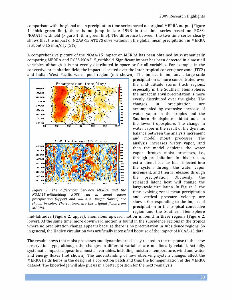
2009 Research Highlights
33
comparison with the global mean precipitation time series based on original MERRA output (Figure 1, thick green line), there is no jump in late 1998 in the time series based on ROSS-‐NOAA15_withheld (Figure 1, thin green line). The difference between the two time series clearly shows that the impact of NOAA-‐15 ATOVS observations in the global mean precipitation in MERRA is about 0.15 mm/day (5%). A comprehensive picture of the NOAA-‐15 impact on MERRA has been obtained by systematically comparing MERRA and ROSS-‐NOAA15_withheld. Significant impact has been detected in almost all variables, although it is not evenly distributed in space or for all variables. For example, in the convective precipitation field, the impact is located over the Inter-‐tropical convergence zone (ITCZ) and Indian-‐West Pacific warm pool region (not shown). The impact in non-‐anvil, large-‐scale
precipitation is more concentrated over the mid-‐latitude storm track regions, especially in the Southern Hemisphere; the impact in anvil precipitation is more evenly distributed over the globe. The changes in precipitation are accompanied by extensive increase of water vapor in the tropics and the Southern Hemisphere mid-‐latitudes in the lower troposphere. The change in water vapor is the result of the dynamic balance between the analysis increment and model moist processes. The analysis increases water vapor, and then the model depletes the water vapor through moist processes, i.e., through precipitation. In this process, extra latent heat has been injected into the system through the water vapor increment, and then is released through the precipitation. Obviously, the released latent heat will change the large-‐scale circulation. In Figure 2, the time evolving zonal mean precipitation and vertical pressure velocity are shown. Corresponding to the impact of precipitation in the tropical convective region and the Southern Hemisphere
mid-‐latitudes (Figure 2, upper), anomalous upward motion is found in these regions (Figure 2, lower). At the same time, more downward motion is found in the subsidence regions in the tropics where no precipitation change appears because there is no precipitation in subsidence regions. So in general, the Hadley circulation was artificially intensified because of the impact of NOAA-‐15 data. The result shows that moist processes and dynamics are closely related in the response to this new observation type, although the changes in different variables are not linearly related. Actually, systematic impacts appear in almost all variables, including moisture, temperature, wind and water and energy fluxes (not shown). The understanding of how observing system changes affect the MERRA fields helps in the design of a correction patch and thus the homogenization of the MERRA dataset. The knowledge will also put us in a better position for the next reanalysis.
Figure 2: The differences between MERRA and the NOAA15_withholding ROSS run in zonal mean precipitation (upper) and 500 hPa Omega (lower) are shown in color. The contours are the original fields from MERRA.

Global Modeling and Assimilation Office
34
On the Nature and Impact of Stationary Rossby Waves During Northern Hemisphere Summer Siegfried Schubert, Hailan Wang, Max Suarez Project Goal: The overall project goal is to assess predictability on subseasonal time scales. Here we focus on the role of stationary Rossby Waves in the development and/or modulation of boreal summer short-‐term climate extremes such as heat waves and flooding events. An example is given showing the impact of the leading stationary wave pattern on the development and modulation of the 2003 heat wave over Europe.
Project Description: The GMAO recently completed more than 30 years of a high-‐resolution reanalysis called the Modern Era Retrospective-‐Analysis for Research and Applications (MERRA). Here we take advantage of these data to examine the nature of summertime precipitation and surface temperature variability on monthly time scales. The initial analysis presented here involves both statistical analyses (correlations, expansion in rotated empirical orthogonal functions or REOFs), and a case study look at the 2003 European heat wave. On-‐going work involves further analysis of these waves in the context of a stationary wave model with idealized forcing.
Results: Figure 1 shows that the precipitation variability in selected locations is not just a local-‐scale convective phenomenon, but in all three cases appears to be associated with wave trains that span much of the Northern Hemisphere. Figure 2 highlights that these are indeed stationary waves
Figure 1: The correlation between the 250 hPa v-wind averaged over the regions (55E-‐70E, 60N-‐70N; 278E-‐290E, 38-‐50N; 263E-‐274E, 38N-‐50N) with precipitation and the v-wind at 250 hPa everywhere (contour interval is 0.1). The data consist of monthly mean anomalies for JJA (1979-2008) in which both the monthly long term mean and the JJA mean for each year are removed. The left panels use GPCP precipitation and the right panels use MERRA precipitation. The v-wind is from MERRA in both. Also shown are the contours of the long-term mean of the JJA 250 hPa u-wind (contours of 15m/s, 20m/s and 25m/s are shown).

2009 Research Highlights
35
(fixed phase). Rough calculations show that the energy (group velocity) propagates to the east at approximately 20m/s.
In order to isolate the wave trains we compute the REOFs of the monthly intraseasonal 250mb v-‐wind anomalies for JJA of 1979-‐2008. Figure 3 shows that the leading patterns consist of well-‐defined waves that span much of the Northern Hemisphere. An inspection of the RPCs (right panel) suggests that these waves may play an important role in a number of climate extremes such as heat waves and flooding events that have occurred over North America and Europe during the last 30 years. Here we focus on the 2003 heat wave over Europe in which REOF 1 appears to play a prominent role. During that summer RPC 1 evolved such that during June it exhibited the most extreme negative value of the last 30 years, it then transitioned to the most extreme positive value in July, and then back to a weak negative value in August. Figure 4 shows the spatial patterns of the precipitation and surface temperature anomalies over Europe and Russia for each month of the heat wave. The results show that June was especially hot, while during July there was some relief, and then August saw a return of the extreme heat. In fact the first 2 weeks of August were especially severe. Comparisons with the evolution of REOF 1 and the associated impacts on precipitation and surface temperature, suggest that this wave played a key role in modulating the temperatures and precipitation, both in contributing to the extreme heat of June and August, and contributing to the amelioration of the heat wave during July. On-‐going work involves the use of a stationary wave model to assess the nature, forcing and potential predictability of this and the other leading stationary wave patterns.
Figure 2: An example of the development of a stationary wave based on the 250 hPa v-wind for JJA (1979-2008) filtered to retain time scales of 30-90 days. The lagged correlations are computed with respect to a base index (an area average of 250 hPa v-wind over Europe). The panels show lags of -8, -4, 0, 4, and 8 days.

Global Modeling and Assimilation Office
36
2003 June (extreme -‐),
July (extreme +)
Figure 3: Left panel: Leading rotated EOFs of the monthly (JJA 1979-2008) intraseasonal v-wind at 250 hPa. Right panel: The associated principal components (RPCs). Units are dimensionless. Note the relatively large amplitude of RPC 1 during 2003, highlighted by a large negative value during June and a large positive value during July.
Figure 4: The left panels show the evolution of the 2003 heat wave over Europe (the 6 upper panels are the precipitation anomalies, and the 6 lower panels are the surface temperature anomalies). The interannual anomalies are deviations from the long term 1979-2008 climatology. For the intraseasonal anomalies the mean JJA for 2003 is also removed. The far right panels show the intraseasonal correlations between RPC 1 (250 hPa v) and precipitation (top panel) and surface temperature (bottom panel), based on the period 1979-2008. Note all panels in Figure 4 are based on MERRA data, though the distributions are very similar to those based on GPCP precipitation and HadCRU TS3.0 surface temperature observations.
2003 June (extreme -‐), July (extreme +)
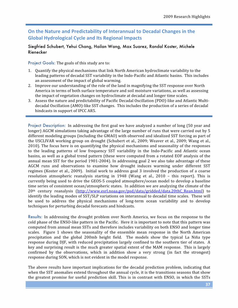
2009 Research Highlights
37
On the Nature and Predictability of Interannual to Decadal Changes in the Global Hydrological Cycle and Its Regional Impacts
Siegfried Schubert, Yehui Chang, Hailan Wang, Max Suarez, Randal Koster, Michele Rienecker Project Goals: The goals of this study are to: 1. Quantify the physical mechanisms that link North American hydroclimate variability to the
leading patterns of decadal SST variability in the Indo-‐Pacific and Atlantic basins. This includes an assessment of the impact of global warming.
2. Improve our understanding of the role of the land in magnifying the SST response over North America in terms of both surface temperature and soil moisture variations, as well as assessing the impact of vegetation changes on hydroclimate at decadal and longer time scales.
3. Assess the nature and predictability of Pacific Decadal Oscillation (PDO)-‐like and Atlantic Multi-‐decadal Oscillation (AMO)-‐like SST changes. This includes the production of a series of decadal hindcasts in support of IPCC AR5.
Project Description: In addressing the first goal we have analyzed a number of long (50 year and longer) AGCM simulations taking advantage of the large number of runs that were carried out by 5 different modeling groups (including the GMAO) with observed and idealized SST forcing as part of the USCLIVAR working group on drought (Schubert et al., 2009; Weaver et al., 2009; Wang et al., 2010). The focus here is on quantifying the physical mechanisms and seasonality of the responses to the leading patterns of low frequency SST variability in the Indo-‐Pacific and Atlantic ocean basins, as well as a global trend pattern (these were computed from a rotated EOF analysis of the annual mean SST for the period 1901-‐2004). In addressing goal 2 we also take advantage of these AGCM runs and observations to examine how drought induces warming under different SST regimes (Koster et al., 2009). Initial work to address goal 3 involved the production of a coarse resolution atmospheric reanalysis starting in 1948 (Wang et al., 2010 – this report). This is currently being used to drive the GEOS-‐5 coupled atmosphere/ocean model to develop a baseline time series of consistent ocean/atmospheric states. In addition we are analyzing the climate of the 20th century reanalysis (http://www.esrl.noaa.gov/psd/data/gridded/data.20thC_Rean.html) to identify the leading modes of SST/SLP variations on interannual to decadal time scales. These will be used to address the physical mechanisms of long-‐term ocean variability and to develop techniques for perturbing decadal forecasts and hindcasts. Results: In addressing the drought problem over North America, we focus on the response to the cold phase of the ENSO-‐like pattern in the Pacific. Here it is important to note that this pattern was computed from annual mean SSTs and therefore includes variability on both ENSO and longer time scales. Figure 1 shows the seasonality of the ensemble mean response in the North American precipitation and the global 200mb height field. The models show the typical La Niña type response during DJF, with reduced precipitation largely confined to the southern tier of states. A key and surprising result is the much greater spatial extent of the MAM response. This is largely confirmed by the observations, which in addition show a very strong (in fact the strongest) response during SON, which is not evident in the model response. The above results have important implications for the decadal prediction problem, indicating that when the SST anomalies extend throughout the annual cycle, it is the transitions seasons that show the greatest promise for useful prediction skill. This is in contrast with ENSO, in which the SSTs

Global Modeling and Assimilation Office
38
tend to peak during boreal winter, with relatively weak amplitude during the other seasons. The 200mb height anomalies (right panels of Figure 1) provide a clue to the greater response during MAM, showing a positive height anomaly over the Pacific with a much more pronounced extension across the U.S. during MAM compared with DJF. This response during MAM appears to be a consistent and robust response among the 5 models. On-‐going work with a stationary wave model suggests this seasonality is in part the result of the seasonality of the zonally-‐symmetric basic state. The lack of a strong response during fall appears to result from model deficiencies in the response over the Caribbean Sea, though the exact nature of that response is still under investigation.
Work towards achieving goal 3 has involved a number of activities aimed at ultimately providing long term atmosphere and ocean data sets for scientific analysis of the mechanisms of decadal variability, and for providing the initial conditions necessary for carrying out our planned decadal hindcasts in support of IPCC AR5. A key effort recently completed was the production of a coarse resolution (2°) reanalysis for the period 1948–present (Wang et al. 2010). This atmospheric dataset is being used to produce a consistent coupled atmosphere/ocean dataset both with and without ocean data assimilation. Hindcasts initialized from the latter will provide a baseline to assess the impact of ocean data. In addition, we are taking advantage of the 20th century reanalysis performed at ESRL to isolate and assess the nature of long-‐term atmosphere/ocean variability. As an example, we show in Figure 2 the two leading complex EOFs of the monthly SST and SLP data for the period
Figure 1: The ensemble mean response computed from 5 different AGCMs (AM2.1, GFSv2, NSIPP-1, CCM3.0, CAM3.5) to an idealized La Niña type SST anomaly (see Schubert et al. 2009). The left panels show the precipitation response (mm/day), and the right panels show the 200mb height response (m). The middle panels are the results of compositing the precipitation observations (1901-2004) for those years during which the amplitude of the La Niña type SST anomaly had an amplitude greater than 1 standard deviation.
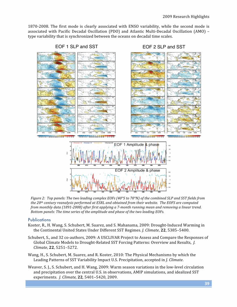
2009 Research Highlights
39
1870-‐2008. The first mode is clearly associated with ENSO variability, while the second mode is associated with Pacific Decadal Oscillation (PDO) and Atlantic Multi-‐Decadal Oscillation (AMO) –type variability that is synchronized between the oceans on decadal time scales.
Publications Koster, R., H. Wang, S. Schubert, M. Suarez, and S. Mahanama, 2009: Drought-‐Induced Warming in
the Continental United States Under Different SST Regimes. J. Climate, 22, 5385–5400.
Schubert, S., and 32 co-‐authors, 2009: A USCLIVAR Project to Assess and Compare the Responses of Global Climate Models to Drought-‐Related SST Forcing Patterns: Overview and Results, J. Climate, 22, 5251–5272.
Wang, H., S. Schubert, M. Suarez, and R. Koster, 2010: The Physical Mechanisms by which the Leading Patterns of SST Variability Impact U.S. Precipitation, accepted in J. Climate.
Weaver, S. J., S. Schubert, and H. Wang, 2009: Warm season variations in the low-‐level circulation and precipitation over the central U.S. in observations, AMIP simulations, and idealized SST experiments. J. Climate, 22, 5401–5420, 2009.
Figure 2: Top panels: The two leading complex EOFs (40°S to 70°N) of the combined SLP and SST fields from the 20th century reanalysis performed at ESRL and obtained from their website. The EOFS are computed from monthly data (1891-2008) after first applying a 7-month running mean and removing a linear trend. Bottom panels: The time series of the amplitude and phase of the two leading EOFs.
EOF 1 SLP and SST EOF 2 SLP and SST

Global Modeling and Assimilation Office
40
The Physical Mechanisms by which the Leading Patterns of SST Variability Impact U.S. Precipitation Hailan Wang, Siegfried Schubert, Max Suarez, Randal Koster Project Goal: The project goal is to use the NASA Seasonal-‐to-‐Interannual Prediction Project (NSIPP-‐1) AGCM to investigate the physical mechanisms by which the leading patterns of annual mean SST variability impact U.S. precipitation. The focus is on a cold Pacific pattern and a warm Atlantic pattern that exert significant drought conditions over the U.S. continent.
Project Description: Recurring patterns of SST variability exert profound impacts on a number of regional climates throughout the world at interannual to decadal and longer time scales. For the United States, the most important SST variations are those associated with El Niño–Southern Oscillation (ENSO) and, at longer time scales, a decadal pan-‐Pacific pattern related to the Pacific decadal oscillation (PDO) and the Atlantic multidecadal oscillation (AMO) in the North Atlantic. A global linear trend pattern and SST variations in the Indian Ocean also appear to be important.
Recent model simulations initiated by the USCLIVAR drought working group (Schubert et al. 2009) provide an opportunity to investigate the mechanisms through which the leading SST patterns affect the regional hydroclimate and to address the issue of the model dependence in representing the linkages between the leading SST patterns and U.S. drought. This study focuses on the results of the USCLIVAR simulations produced by the NSIPP-‐1 AGCM, and examines the physical and dynamical mechanisms through which the cold Pacific and warm Atlantic SST patterns influence U.S. precipitation. In particular, we address the reasons for the similarity in the warm season precipitation responses over the Great Plains to the cold Pacific and warm Atlantic, and the causes for the distinct seasonality in the Southeast (SE) U.S. precipitation response to the cold Pacific.
Results: The precipitation response to the cold Pacific (Figure 1 upper panels) is characterized by persistent deficits over the Great Plains that peak in summer with a secondary peak in spring, and weakly pluvial conditions in summer over the SE U.S. The precipitation response to the warm Atlantic (Figure 1 lower panels) is dominated by persistent deficits over the Great Plains with the maximum deficit occurring in late summer. The precipitation response to the warm Atlantic is overall similar to the response to the cold Pacific with, however, considerably weaker amplitude.
An analysis of the atmospheric moisture budget combined with a stationary wave model diagnosis of the associated atmospheric circulation anomalies was conducted to investigate mechanisms of
Figure 1: Seasonal mean precipitation responses (mm day−1) to the cold Pacific (upper panels) and warm Atlantic (lower panels) SST patterns, for DJF, MAM, JJA, and SON in the idealized experiments performed using the NASA NSIPP-1 AGCM. Regions with responses that are significant at the 5% level based on a t test are indicated using contours.

2009 Research Highlights
41
the precipitation responses. A key result is that, while the cold Pacific and warm Atlantic are two spatially distinct SST patterns, they nevertheless produce similar diabatic heating anomalies over the Gulf of Mexico during the warm season (Figure 2). For the Atlantic forcing case, the heating anomalies are a direct response to the SST anomalies, whereas for the Pacific forcing case they are a secondary response to circulation anomalies forced from the tropical Pacific. The diabatic heating anomalies in both cases force an anomalous low-‐level cyclonic flow over the Gulf of Mexico (Figure 2) that leads to reduced moisture transport into the central U.S. and increased moisture transport into the eastern U.S. (Figure 3 lower panels). The precipitation deficits over the Great Plains in both cases are greatly amplified by the strong soil moisture feedback in the NSIPP-‐1 AGCM (Figure 3 middle panels). In contrast, the response over the SE to the cold Pacific during spring (not shown) is primarily associated with an upper-‐tropospheric high anomaly over the southern U.S. that is remotely forced by tropical Pacific diabatic heating anomalies, leading to greatly reduced stationary moisture flux convergences and anomalous subsidence in that region. Moderately reduced evaporation and weakened transient moisture flux convergences play secondary roles. It is only during spring that all three terms are negative and produce the maximum dry response in spring.
The above findings based on the NSIPP-‐1 AGCM are generally consistent with observations, as well as with four other AGCMs included in the U.S. CLIVAR project.
Publications Schubert, S., H. Wang, R. Koster, M. Suarez, S. Weaver, and co-‐authors, 2009: A USCLIVAR Project to
Assess and Compare the Responses of Global Climate Models to Drought-‐Related SST Forcing Patterns: Overview and Results, J. Climate, 22, 19, 5251–5272.
Wang H., S. Schubert, M. Suarez and R. Koster, 2010: The Physical Mechanisms by which the Leading Patterns of SST Variability Impact U.S. Precipitation. J. Climate, 23, 7, 1815–1836.
Figure 3: The atmospheric moisture budget analysis for the JJA response to a cold Pacific pattern in the standard idealized run (left) and the auxiliary run that has the soil moisture feedback turned off (right), performed using the NSIPP-1 AGCM. The responses of precipitation (upper panels), evaporation (middle panels), and vertically integrated stationary moisture flux convergences due to the changes in atmospheric circulation superimposed with the corresponding vertically integrated stationary moisture fluxes (lower panels) are shown. The reference vector is shown below the lower left panel. Units: mm day−1. The moisture budget for the JAS response to a warm Atlantic pattern is overall similar to that for cold Pacific in JJA, and is not shown here.
Figure 2: The eddy streamfunction (m2 s−1) at σ = 0.866 in the AGCM responses to the cold Pacific in JJA (upper left) and the warm Atlantic in JAS (upper right); the stationary wave model response to regional diabatic heating anomalies over the local tropical Atlantic and U.S. for Cold Pacific in JJA (lower left), and warm Atlantic in JAS (lower right). The corresponding vertically integrated diabatic heating anomalies (K day−1) are shaded. The streamfunction contour interval is 0.5 × 10⁶ m2 s−1 (negative values are dashed and the zero line is the first solid contour).

Global Modeling and Assimilation Office
42
The Post-‐war (1948-‐1978) Extension of the MERRA Scout
Hailan Wang, Siegfried Schubert, Austin Conaty, Meta Sienkiewicz, Douglas Collins Project Goals: The primary goal of this project was to produce a 60+ year coarse resolution (2°×2.5°) reanalysis by extending the existing MERRA Scout back in time to cover the period 1948-‐1978. An additional goal was to perform an initial evaluation of the characteristics of the extended (1948-‐present) reanalysis, including an assessment of the impact of the changing observing system.
Project Description: The so-‐called MERRA Scout was initially produced as part of the preparation for MERRA production, as a quick way to look ahead and identify problems with the observations during the satellite era (1979-‐present). In view of the GMAO plans to address issues involving decadal variability and predictability, it was decided to extend the Scout reanalysis back in time to cover the period (1948-‐1978), thus providing a relatively inexpensive (compared with MERRA) yet scientifically valuable dataset spanning six decades. The Scout experiment uses the same observations and the same data assimilation system as in MERRA, with the primary difference being the spatial resolution. The observational data for the period 1948-‐1978 were provided by NCEP EMC, and consist largely of conventional observations. Results: The observations for the period 1948-‐1978 undergo significant changes with time (Figure 1). Not only does the observational network get denser, but more conventional observational data types become available. These observations include radiosonde (1948-‐present), surface land station (1948-‐present), surface marine observations (1948-‐present), PIBAL winds (1948-‐present), aircraft (MDCARS, ASDAR, AIREP/PIREP, Dropsonde) reports (1962-‐present), cloud drift winds (METEOSAT, GMS, GOES) (1977-‐present) and Australian PAOB (1978-‐present). The observations are mainly in the Northern Hemisphere (NH), with the majority over the NH land.
Figure 1: The changing observing system during 1948-1978.
0Z 15 Jan 1950 0Z 15 Jan 1960
0Z 15 Jan 1970 0Z 15 Jan 1978
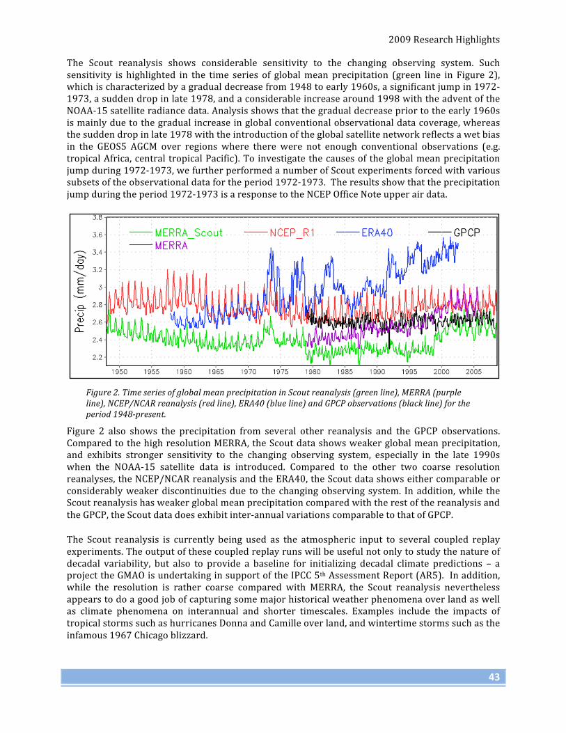
2009 Research Highlights
43
The Scout reanalysis shows considerable sensitivity to the changing observing system. Such sensitivity is highlighted in the time series of global mean precipitation (green line in Figure 2), which is characterized by a gradual decrease from 1948 to early 1960s, a significant jump in 1972-‐1973, a sudden drop in late 1978, and a considerable increase around 1998 with the advent of the NOAA-‐15 satellite radiance data. Analysis shows that the gradual decrease prior to the early 1960s is mainly due to the gradual increase in global conventional observational data coverage, whereas the sudden drop in late 1978 with the introduction of the global satellite network reflects a wet bias in the GEOS5 AGCM over regions where there were not enough conventional observations (e.g. tropical Africa, central tropical Pacific). To investigate the causes of the global mean precipitation jump during 1972-‐1973, we further performed a number of Scout experiments forced with various subsets of the observational data for the period 1972-‐1973. The results show that the precipitation jump during the period 1972-‐1973 is a response to the NCEP Office Note upper air data.
Figure 2 also shows the precipitation from several other reanalysis and the GPCP observations. Compared to the high resolution MERRA, the Scout data shows weaker global mean precipitation, and exhibits stronger sensitivity to the changing observing system, especially in the late 1990s when the NOAA-‐15 satellite data is introduced. Compared to the other two coarse resolution reanalyses, the NCEP/NCAR reanalysis and the ERA40, the Scout data shows either comparable or considerably weaker discontinuities due to the changing observing system. In addition, while the Scout reanalysis has weaker global mean precipitation compared with the rest of the reanalysis and the GPCP, the Scout data does exhibit inter-‐annual variations comparable to that of GPCP.
The Scout reanalysis is currently being used as the atmospheric input to several coupled replay experiments. The output of these coupled replay runs will be useful not only to study the nature of decadal variability, but also to provide a baseline for initializing decadal climate predictions – a project the GMAO is undertaking in support of the IPCC 5th Assessment Report (AR5). In addition, while the resolution is rather coarse compared with MERRA, the Scout reanalysis nevertheless appears to do a good job of capturing some major historical weather phenomena over land as well as climate phenomena on interannual and shorter timescales. Examples include the impacts of tropical storms such as hurricanes Donna and Camille over land, and wintertime storms such as the infamous 1967 Chicago blizzard.
Figure 2. Time series of global mean precipitation in Scout reanalysis (green line), MERRA (purple line), NCEP/NCAR reanalysis (red line), ERA40 (blue line) and GPCP observations (black line) for the period 1948-present.

Global Modeling and Assimilation Office
44
Interannual Variability of the African Easterly Jet and Easterly Waves and Associated Weather and Climate Man-Li Wu, Siegfried Schubert, Max Suarez, Randy Koster, Chris Thorncroft (SUNY/Albany), Oreste Reale (Code 613), Winston Chao Project Goal: The goal of this project is to obtain an integrative understanding of Atlantic storm and hurricane development and West African Monsoon rainfall. In doing so, we make extensive use of the Modern Era Retrospective-‐Analysis For Research And Applications (MERRA) products together with the Goddard Earth Observing System model version 5 (GEOS-‐5).
Project Description: MERRA is being used together with the GEOS-‐5 model to investigate the controls of the inter-‐annual variability of the African Easterly Jet (AEJ), Waves (AEWs) and associated weather and climate systems. We focus on the following: (1) the AEJ, (2) the AEWs, (3) their downstream effects, (4) the relative role of the AEWs and the Atlantic environment in cyclogenesis and storm/hurricane tracks, and (5) the relationship between the AEJ and AEWs and the West African Monsoon (WAM) rainfall. Results from MERRA are compared with those from other reanalyses: ERA-‐40, NCEP/DOE Reanalysis 2 (NCEP-‐R2), and the Japanese 25-‐year Reanalyses (JRA-‐25). Results: We have analyzed MERRA, ERA-‐40, NCEP-‐R2, and JRA-‐25 data for the period 1980 through 2001. All the reanalyses produce a reasonable AEJ, and all reanalyses reveal similar mechanisms that control the interannual variability of the AEJ and AEWs. However they do differ in the details. For example, the AEJ is strongest in MERRA (12m/s), and weakest in JRA-‐25 (10m/s). The northern portion of the AEJ is strongest in MERRA and the southern portion of the AEJ is strongest in NCEP. Due to differences in the basic structure of the jet, the AEW activity is different as a result of differences in the meridional gradient of the jet and absolute vorticity around the Jet. JRA-‐25 has the weakest AEW activity over land. We also found that barotropic instability alone appears to strongly constrain the location where storms occur and therefore appears as a potential predictor of tropical cyclone genesis on seasonal time scales. In terms of the mechanisms that control the interannual variability of the AEJ/AEWs, the impact of ENSO, MJO, a strong or weak jet, and the local SSTA have been examined. All four reanalyses reveal similar impacts from those mechanisms, but they again differ in detail. During La Niña years, the AEJ extends further north in all four reanalyses. There is also stronger AEW activity during La Niña years. The analyses also show that a stronger AEJ leads to more active AEWs. However, the local SSTA impact on the AEWs appears to be weak. The impact of the MJO (for ENSO neutral years) is to produce a substantial increase in variance during its negative phase. We are currently examining the wave and jet interactions over the Atlantic. This includes an assessment of the extent to which the jet acts as a wave guide for the AEWs, the energy conversions between the jet and the waves, and the possible mid-‐latitude impacts on the AEWs. Publication Wu, Man-‐Li C., O. Reale, S. D. Schubert, Max. J. Suarez, C. Thorncroft, 2010: African Easterly Jet:
barotropic instability, waves and cyclone development (draft).

2009 Research Highlights
45
GLACE-‐2 -‐ The Second Phase of the Global Land-‐Atmosphere Coupling Experiment Randal Koster, Sarith Mahanama and 21 contributors from multiple institutions Project Goal: GLACE-‐2, the second phase of the Global Land-‐Atmosphere Coupling Experiment, is aimed at quantifying, across a broad suite of state-‐of-‐the-‐art forecast models, the subseasonal (out to 60 days) forecast skill associated with the initialization of land surface state variables. GMAO personnel are coordinating the international experiment and are taking the lead in processing the results.
Project Description: A handful of studies have examined the impact of initializing a forecast system with observations-‐based estimates of soil moisture, with generally optimistic results. These studies, however, are uncoordinated, model-‐specific, and very difficult to compare given their different forecast periods and sample sizes and their different verification metrics. In GLACE-‐2, the same numerical experiment, one specifically designed to isolate soil moisture initialization impacts on subseasonal forecast skill (measured against real observations, with a high number of independent start dates for robust statistics), is performed with ten independent forecast systems. The result is a coordinated “consensus” view of the degree to which realistic land initialization improves forecast quality in today’s models. Participants in GLACE-‐2 performed two series of 2-‐month, 10-‐member ensemble forecasts covering a wide range of boreal warm-‐season start dates: 10 start dates per year (April 1, April 15, May 1, ... August 15) for each year in 1986-‐1995. The two series differ from each other only in the nature of their land surface initialization. In Series 1, land conditions (particularly soil moisture) are initialized to realistic values based on an offline integration of historical meteorological forcing. In Series 2, realistic land surface initialization is not utilized. Forecasted 15-‐day precipitation and air temperature averages are compared to the corresponding observations, with skill measured as the square of the correlation coefficient between them; by subtracting the forecast skill obtained for Series 2 from that obtained for Series 1, we isolate the impacts of soil moisture initialization on the skill. All forecasts performed in GLACE-‐2 are true forecasts. The GLACE-‐2 experiments were performed with ten modeling systems: those of the Canadian Centre for Climate Modelling and Analysis (CCCma), the Center for Ocean-‐Land-‐Atmosphere Studies (COLA), the European Centre for Medium-‐Range Weather Forecasts (ECMWF), the European Centre/Hamburg forecast system (ECHAM), Florida State University/Center for Ocean-‐Atmosphere Prediction Studies (FSU/COAPS), Geophysical Fluid Dynamics Laboratory (GFDL), the GMAO (pre-‐GEOS-‐5 system), the National Center for Atmospheric Research (NCAR; two contributions), and the National Centers for Environmental Prediction (NCEP). Together these systems represent the state-‐of-‐the-‐art in atmospheric modeling and prediction. Results: Figure 1 shows multi-‐model “consensus” results for air temperature prediction at the 30-‐day lead (days 31-‐45) for time periods during June-‐August. This is a measure of the contribution of realistic land initialization to air temperature forecast skill, averaged across the models. The top panel shows the skill contributions when all start dates are considered. Realistic land initialization contributes about 0.05 to the r2 skill score over many parts of the northern U.S. The bottom panel shows the corresponding skill contributions obtained when only the driest and wettest start dates (bottom and top 20%, in terms of initial local soil moisture) are included in the skill calculation. The skill contributions jump to 0.15 or more in some places for this conditional calculation; soil

Global Modeling and Assimilation Office
46
moisture initialization thus has a more significant impact on skill when the initial anomaly is relatively large. For the most part, the values shown in the maps differ from zero at a confidence level of 95% or more. See the GRL reference for a more precise discussion of significance.
Skill levels obtained for precipitation at the same lead are substantially weaker (Figure 2), but the land contribution is still significantly different from zero at the 95% confidence level in many places. Though these levels are weak, the difficulty of producing forecasts with any skill at all at these leads must be kept in mind. Summer rainfall prediction skill at subseasonal leads has always been an elusive goal. Several GLACE-‐2 analyses are still underway. Results are beginning to show how the rain gauge density underlying the land initialization has a major impact on the skill levels produced, highlighting the value that a mission like GPM, in combination with a soil moisture mission like SMAP, may have on operational forecasting. GLACE-‐2 is co-‐sponsored by CLIVAR and GEWEX, which are both arms of the World Climate Research Program (WCRP). URL: http://gmao.gsfc.nasa.gov/research/GLACE-‐2 Publications Koster, R. D., Mahanama, S. P. P., and 21 co-‐authors, 2010: Contribution of land surface initialization
to subseasonal forecast skill: First results from a multi-‐model experiment. Geophys. Res. Lett., 37, L02402, doi:10.1029/2009GL041677.
Koster, R. D., Mahanama, S. P. P., and 21 co-‐authors, in preparation: The second phase of the Global Land-‐Atmosphere Coupling Experiment. To be submitted to J. Hydromet.
Figure 2: Same as Figure 1, but for precipitation forecast skill at the 30-day lead.
Figure 1: Multi-model consensus view of land contribution to air temperature forecast skill at the 30-day lead (days 31-45). Top: Skill contribution based on all 15-day averaging periods during JJA. Bottom: Skill contribution based only on those periods for which initial soil moistures were particularly wet or dry.

2009 Research Highlights
47
Simulating and Predicting Sub-‐seasonal and Longer-‐Term Changes in Tropical Storm Characteristics using High Resolution Climate Models Siegfried Schubert, Max Suarez, Myong-In Lee, Man Li Wu, Oreste Reale, Julio Bacmeister Project Goals: The goals of this study are to: 1. Improve the ability of the GEOS-‐5 model to simulate tropical storms. In particular, we assess
the sensitivity to resolution and the convective and boundary layer schemes, and develop and assess methods for verifying storms at a range of model resolutions.
2. Improve our understanding and simulation of the link between tropical storm characteristics and a) the MJO and b) the leading patterns of SST variability including those associated with ENSO, the AMO, and the 20th century climate trend.
3. Carry out a series of hindcasts with the coupled atmosphere-‐ocean-‐land GEOS-‐5 model to assess the skill of subseasonal to seasonal forecasts of tropical storm characteristics.
Project Description: In addressing the first goal we have examined the sensitivity to the cumulus parameterization scheme of the daily precipitation variability in the GEOS-‐5 AGCM by gradually turning off the cumulus scheme. In addition, we assessed the impact of incorporating a stochastic treatment of cumulus entrainment – the so-‐called “stochastic Tokioka” scheme. Initial work to address goal two consisted of running an ensemble of AGCM simulations for different hurricane seasons to examine the impact of the SST using the version of the GEOS-‐5 model found to produce the most realistic precipitation variability. Further results from these runs as well as those from other modeling groups conducting high-‐resolution simulations can be found in Schubert et al. (2009). Results: As a first step we examined the impact of gradually reducing the influence of the cumulus parameterization in the GEOS-‐5 AGCM. This was achieved by increasing the relaxation time scale of the Relaxed Arakawa-‐Schubert (RAS) scheme from 6 hours to 12 hours and finally to 11.2 days. The results show that the percent of the tropical and subtropical precipitation produced by RAS (in the convectively active regions) changes from roughly greater than 60% for the standard time scale, to 40-‐60% for the 12-‐hour time scale, to basically zero when the time scale is increased to 11.2 days. The impact of those changes on the daily precipitation variability is shown in Figure 1. The results show that the standard 6-‐hour time scale produces too weak variability compared with GPCP. On the other hand, when RAS is basically shut off (time scale of 11.2 days), the precipitation variability becomes unrealistically large. The 12-‐hour time scale seems to produce the most realistic variability. The results are similar for both resolutions, though the 25km resolution appears to produce somewhat noisier and widespread regions of high precipitation variability. Figure 2 shows the impact of the stochastic Tokioka scheme on the organization of tropical precipitation. The results suggest that the stochastic treatment of the entrainment appears to produce better organization in the tropical precipitation including the eastward propagation that is typically associated with the Madden Julian Oscillation. Further results from the runs with the stochastic Tokioka scheme (not shown) indicate that the simulated hurricanes (at 25km) have a very realistic warm core and spatial scales, with the strongest storm exhibiting near surface winds exceeding 60m/s and a minimum pressure of 960 mb.

Global Modeling and Assimilation Office
48
In view of the above results an ensemble of five 50-‐km (1/2 degree) seasonal simulations (with specified SST) were carried out with a version of the GEOS-‐5 AGCM that includes the stochastic Tokioka scheme, and a RAS relaxation time scale of 12 hours. In particular, runs were made for 1997, 1998, 1999, 2004, 2005, 2006, 2007, with each run initialized on 15 May and run out to 1 December. The years cover a strong El Niño, a strong La Niña, as well as the record-‐breaking hurricane season of 2005. The results in Figure 3 show that the model does a reasonable job of reproducing the interannual variability of the number of tropical storms. While the model does not reproduce the record 27 observed storms during 2005, it does show considerable intra-‐ensemble variability, with one ensemble member producing 22 storms. On-‐going work suggests that higher resolution (e.g., 14km) is necessary to simulate the most extreme storms (hurricanes with category 5 intensities), and to produce more realistic seasonal storm counts.
Figure 1: The daily precipitation variability during JJA in the GEOS-5 AGCM run at 25 and 50km resolution with several different relaxation time scales (the standard 6 hours, 12 hours and 11.2 days) of the Relaxed Arakawa-Schubert (RAS) scheme. The top panel shows the result from the GPCP observations.
GPCP Observations
50-km Resolution Simulations
25-km Resolution Simulations

2009 Research Highlights
49
Publication Schubert, S.D., I.-‐S. Kang, F. Kucharski, J. Shukla, 2009. Summary Report of the Workshop on High-‐
Resolution Climate Modeling, Abdus Salam International Centre for Theoretical Physics (ICTP), Trieste, Italy, 10-‐14 August 2009. Available at: http://gmao.gsfc.nasa.gov/pubs/conf/
Figure 3: Number of observed and simulated storms using an early version of GEOS-5 at ½° resolution and a modified version of RAS (stochastic Tokioka). Model runs were done for 1997, 1998, 1999, 2004, 2005,2006,2007 with integrations beginning on 15 May and ending 1 December.
Figure 2: Hovmuller diagrams of the precipitation averaged between 10°S and10°N, for the control (left panel), the run with the stochastic Tokioka scheme (middle panel) and the GPCP observations (right panel).

Global Modeling and Assimilation Office
50
Role of Upper-‐Level Jet Dynamics in Extreme 10-‐Day Warm Season Flood Events over the North-‐Central United States
H. Mark Helfand, Siegfried Schubert Project Goal: The goal of this research is to better understand the physical basis for warm-‐season hydroclimatic variability over the north-‐Central United States, and specifically to investigate the influence of the upper-‐level Pacific/North American Jet on the occurrence of extreme warm-‐season flooding events over this region on the pertinent time scale.
Project Description: Based on the similarity of precipitation anomalies and upper-‐level dynamics for the flooding events of July 1993 and June 2008, the pertinent time scale for these events was taken to be ten days. The ten largest 10-‐day warm-‐season (MJJA) precipitation anomalies over the Northern Great Plains region (40°-‐48°N; 87.5°-‐105°W) were objectively chosen for the 61-‐year period from 1948-‐2008. Anomalous fields (from the 60-‐year climatology for the years 1948-‐2007 from the NCEP/NCAR Reanalysis 1) for these ten cases were composited together by using the first day of each 10-‐day precipitation anomaly event as a reference time. Statistical significance masks, Hovmoller diagrams, and digital filtered time series have been used to analyze the evolution of the ensemble composite time series.
Figure 1: Wind anomaly vectors (90% confidence level, gray; 95%, black), vorticity anomalies (90% confidence level, red positive, blue negative) and unmasked total wind speed (shaded, climatology in purple). Results: A statistically significant signal first shows up in the 250 hPa vorticity anomaly field 9 days before the onset (DBO) of the flood (Figure 1a). A Rossby wave clearly can be discerned by 3 DBO as

2009 Research Highlights
51
an arching, 3-‐cell wave train (Figure 1d) and then a zonally oriented wave across North America (by 1 DBO, Figure 1e). A far-‐western kink in the wave generates a divergence center that propagates along the jet toward the Great Plains where it initiates and supports intense flooding. The jet broadens as it arches deeply into the Gulf of Alaska (Figures 1f-‐h) and finally begins to attenuate by 7 DAO (Figure 1i). Figure 2 shows 8-‐day low-‐pass filtered anomaly fields indicating a persistent, 5-‐period quasi-‐stationary wave from Asia to Europe. Further analysis (not shown) suggests that the change in phase of this wave from 20 DBO to 0 DBO may be driven by intraseasonal variability of tropical convection (MJO) in the Indian and west Pacific Oceans. Comparison of 250 to 850 hPa meridional wind anomalies (Figures 2c and d) shows the propagating upper-‐level jet causing the Great Plains Low Level Jet and its northward moisture flux to accelerate as the upper and lower level flows lock into a deep, standing-‐wave pattern 3days after the onset of the nominal flooding period.
Figure 2: Hovmoller diagrams for meridionally averaged 8-day, low-pass composite anomalies (red positive, blue negative) over the region between Asia and Europe. Horizontal black lines denote the temporal limits of the period of flooding. Vertical black lines delimit the geographic region of highest interest. Gold, yellow, and gray shading denote 99%, 90%, and 80% confidence levels. Publication Helfand, H.M., 2010: Impact of the Pacific/North American Jet on large, ten-‐day, warm-‐season
flooding episodes over the northern Great Plains of the United States. To be submitted to J. Climate.

Global Modeling and Assimilation Office
52
Real-‐Time Biomass Emissions for Environmental Forecasting Arlindo da Silva, Ravi Govindaraju Project Goal: The project goal is develop real time and retrospective estimates of biomass burning emissions for use in the GEOS-‐5 climate system model in support of aerosol forecasting and data assimilation.
Project Description: Unlike the forecasting of traditional meteorological parameters where the first order of business is an accurate determination of initial conditions, environmental parameters such as atmospheric aerosols are primarily boundary forced. As such, accurate determination of emissions, combined with realistic transport mechanisms, is critical for skilful forecasting. Biomass emissions from natural and manmade fires are an important source of atmospheric aerosols and other pollutants. Broadly speaking, satellite-‐based estimates of biomass burning emissions start with the determination of thermal anomalies or “hot spots” (i.e., those pixels that are sufficiently hotter than their surroundings). In the so-‐called bottom-up methods, the emissions are made proportional to the fire pixel counts, with the proportionality constant dependent on detailed information about the material being consumed and the area burned. Much of these supplementary metadata are obtained from existing inventories that are not always very reliable. For a particular hot spot at a given longitude, λ, latitude, φ, and time, t, the mass Mx of emitted species x can be written as Mx(λ,φ) = px(λ,φ) A(λ,φ) (1) where A is the satellite derived fractional area of the pixel being burned, and the coefficient px is the for species x that depends on the emission factor, biomass density, the fuel type, the burning efficiency, and other factors. Much of the spatial dependency of the emissions comes from px and is not directly observed by satellite. On the other hand, in the top-down approach the mass of emitted species x can be directly related to the fire radiative energy measured by the satellite (e.g., Ichoku and Kaufman, 2005): Mx(λ,φ) = Cx,bRFRE(λ,φ) (2) where RFRE is the (satellite measured) fire radiative energy (FRE) and Cx,b is the FRE-‐based emission coefficient, a quantity which can be measured in the laboratory (Wooster, 2002). To a good approximation Cx,b is only a function of the biome type, b, being consumed. In this formulation, most of the spatial/temporal dependency in the emissions comes from satellite measurements rather than from prescribed inventories. The MODIS sensor on the EOS/Terra satellite is the first to operationally measure FRE from space. FRE is determined from the MODIS 3.96-‐ and 11-‐ micron channels, which do not saturate for most fires. The MODIS Active Fire Product (Giglio, 2005) provides retrievals of FRE for each fire pixel detected. For the purpose of global modeling, we use the IGBP landcover database for classifying each burning pixel in 4 broad biome types: tropical forests, boreal forests, savannah and grasslands. Thus, for each model gridbox, (i,j), the emission rate for species x can be written as Ex(i,j) = Σb Cx,b Rb(i,j) (3) where Cx,b is a biome-‐dependent global constant, and Rb is the FRE summed over all burning pixels in gridbox (i,j) having biome type b. Rather than prescribing Cx,b from first principles or lab

2009 Research Highlights
53
measurements we adopt here the pragmatic approach of having these 4 constants as tunable parameters to be adjusted within a modeling context.
Results: One simple approach is to choose Cx,b in such way as to match the long term means of global emissions by some established biomass emission inventories, e.g., the Global Fire Emission Database of van der Werf et al. (2006). As illustrated in Figure 1, MODIS FRE based estimates can be tuned to a high degree of correlation with GFED estimates: each point in this diagram is the global monthly mean for each biome. Another strategy for tuning Cx,b consists of adding tagged tracers to GEOS-‐5, each having the individual Rb as sources. Using standard inverse techniques Cx,b can be determined by minimizing the discrepancy between the tracer mixing ratio and some observational dataset, for example AIRS CO retrievals. Notice that once Cx,b is determined for a given species
x, it can be scaled for another species using as reference emissions factors such as those in Andreae and Merlet (2001). We have also implemented a pyro-‐cumulus parameterization to physically determine the smoke injection layer. The 1D plume rise model of Freitas et al. (2006, 2007) predicts the bottom and top of the smoke layer based on the GEOS-‐5 meteorological parameters and the fire characterization afforded by our new emission algorithm. Having the correct injection layer is crucial for accurate transport of biomass burning aerosols and subsequent interaction with the circulation. We are currently evaluating these emissions in GEOS-‐5 for the EOS period (2000-‐2009). References Andreae, M., and P. Merlet, 2001: Emission of trace gases and aerosols from biomass burning. Global
Biogeochem. Cyc. , 15 (4), 955-‐966.
Freitas, S., K. Longo, and M. Andreae, 2006: Impact of including the plume rise of vegetation fires in numerical simulations of associated atmospheric pollutants. Geophys. Res. Lett. , 33 (17), L17808.
Freitas, S., K. Longo, R. Chatfield, D. Latham, M. Silva Dias, M. Andreae, and co-‐authors, 2007: Including the sub-‐grid scale plume rise of vegetation fires in low resolution atmospheric transport models. Atmos. Chem. Phys. , 7 (13), 3385-‐3398.
Giglio, L., 2005: MODIS Collection 4 Active Fire Product User’s Guide. Version 2.2 (available at: http://modis-fire.umd.edu/documents/MODIS_Fire_Users_Guide_2.2.pdf)
Ichoku, C., and Y. J. Kaufman, 2005: A method to derive smoke emission rates from MODIS fire radiative energy measurements. IEEE Trans. Geosci. & Rem. Sens., 43 (11), 2636-2649.
Van der Werf, G., J. Randerson, L. Giglio, G. Collatz, P. Kasibhatla, and A. Arellano, 2006: Interannual variability in global biomass burning emissions from 1997 to 2004. Atmos. Chem. Phys. , 6, 3423-‐3441.
Wooster, M., 2002: Small-‐scale experimental testing of fire radiative energy for quantifying mass combusted in natural vegetation fires. Geophys. Res. Lett., 29 (21), 2027, doi:10.1029/2002GL015487.
Figure 1: MODIS Fire Radiative Energy versus GFED v2 emissions.

Global Modeling and Assimilation Office
54
The Impact of Stratosphere-‐Troposphere Exchange on Surface CO2 Mixing Ratios Studied with the GEOS-‐5 AGCM
Lesley Ott, Steven Pawson Project Goal: The project goal is to better understand how stratosphere-‐troposphere exchange (STE) processes may influence surface CO2 mixing ratios. Such processes are known to exert a strong influence on tropospheric ozone mixing ratios and photochemistry and several recent studies have demonstrated that STE also affects CO2 in the upper troposphere. However, the representation of STE can vary widely between models and contains significant uncertainty. Because surface CO2 mixing ratios are frequently used to estimate CO2 sources and sinks, understanding the relevant processes and their associated uncertainties is critically important to carbon cycle research.
Project Description: The GEOS-‐5 AGCM calculates the global distribution of CO2 mixing ratios online using specified distributions of surface fluxes from fossil fuel combustion, biomass burning, oceans, and the terrestrial biosphere. In order to examine the impact of stratosphere-‐to-‐troposphere transport (STT) on surface CO2 mixing ratios, we have implemented a package of stratospheric CO2 and air mass tracers in GEOS-‐5. In addition to being ‘tagged’ by stratospheric origin, these tracers are also tagged by the calendar month in which they were transported across the tropopause and followed for three subsequent months to examine transport timescales. Stratospheric tracers are removed from the model domain when an air parcel re-‐enters the stratosphere or is drawn down into the surface by ocean or biosphere exchange. A 10-‐year simulation was completed in order to examine interannual differences in transport. STT tracers were also used to estimate the influence on surface CO2 mixing ratios if STT were overestimated in the model.
Results: The impact of STT on surface mixing ratios depends strongly on both the seasonal cycles of surface CO2 mixing ratios and the seasonal cycles of CO2 mixing ratios in the vicinity of the tropopause. Near the tropopause, CO2 mixing ratios typically display a seasonal cycle that is weaker than the cycle at the surface and often lag changes at the surface, especially in regions where transport is not dominated by strong convection. STT transport also displays a pronounced seasonal cycle with the strongest transport of stratospheric air evident in the midlatitudes of each hemisphere during winter months.
Figure 1: Top plots show the monthly mean percentage of air transported from the stratosphere to the surface during the current and previous calendar month. Bottom plots show the difference, in ppmv, between surface and tropopause CO2 mixing ratios in February, May, and August, 2002.

2009 Research Highlights
55
Figure 1 shows the model calculated percentage of air near the surface which has been transported across the tropopause during the current and previous calendar months as well as the difference between surface and tropopause CO2 mixing ratios. The greatest spatial variability of the stratospheric air mass tracer is found ~30-‐60 days following the time of the STT. As the time from the STT is extended past 60 days, spatial variations in the percentage of this stratospheric air at the surface diminish. The strongest vertical CO2 gradients are found in source regions over North America, Europe and Asia. Positive gradients indicate that the surface CO2 is greater than the tropopause mixing ratio. Peak gradient values occur during January when NH surface CO2 mixing ratios are high due to fossil fuel and biosphere fluxes. In July, the largest negative values are found in the same areas as they experience strong drawdown of CO2 at the surface. In the SH, weaker fluxes lead to less seasonal variability in the vertical gradient of CO2.
Figure 2 shows estimates of several types of errors that could be introduced into surface CO2 mixing ratios through errors in large-‐scale transport and mixing processes. For example, the model could overestimate the fraction of air at the surface that was recently transported from the stratosphere. If we assume that the vertical gradient of CO2 is simulated correctly but the magnitude of STT is overestimated by 50%, simulated CO2 mixing ratios at the surface would change by more than 1 ppmv over CO2 source regions in North America, Europe and Asia during February. In these regions, STT reduces surface mixing ratios by transporting air with lower CO2 mixing ratios downward. During August, reduction in STT would slightly decrease CO2 mixing ratios over North America and Europe but in most locations this change would be less than 0.5 ppmv. If instead we assume that STT is reasonable but that the vertical gradient of CO2 is underestimated, differences are of nearly equal magnitude but opposite in sign. This work underscores the important role that STT plays in influencing surface CO2 mixing ratios. Concurrent analysis of simulated ozone will be used to identify and evaluate simulated STT in GEOS-‐5. Future research will examine how errors introduced by uncertainty in STT propagate into CO2 source and sink estimates using inversion techniques.
Figure 2: Plots at left show estimates of several types of error in surface CO2 mixing ratios that could be caused by errors in large-scale vertical transport for February and August 2002. Top plots show the change in surface CO2 if the vertical gradient of CO2 is unchanged but the magnitude of STT is reduced by 50%. Bottom plots show the surface CO2 change if the magnitude of STT is unchanged while the vertical gradient of CO2 is increased by 50%.

Global Modeling and Assimilation Office
56
GEOS-‐5 Near Real-‐time Data Products
Gi-Kong Kim, Al Ruddick, Robert Lucchesi, Austin Conaty Project Goals: The GEOS-‐5 data assimilation system (DAS) products are generated to support remote sensing data retrieval and Earth system science research in the areas of climate and weather prediction, observing system modeling and design, and basic research in atmospheric processes. The objectives of this project are 1) to perform end-‐to-‐end testing of the GEOS-‐5 data production system under development, and 2) to maintain the near real time production as well as retrospective processing of the GEOS-‐5 DAS products and 5-‐day forecasts.
Project Description: The GEOS-‐5 analysis products and forecasts are generated daily in near real time using high-‐end computing (HEC) resources at the NCCS and distributed to the user community via the GES DISC. The GEOS-‐5 data, with a limited retention period, are made available on a data portal at NCCS for non-‐operational users and also for the customized real time support for field campaigns. The current user community includes EOS instrument teams (MODIS/Land, CERES, MLS, TES, and CALIPSO); other NASA Projects (POWER, FLASHFlux, Flood Warning); University Research Groups (GEOS-‐CHEM at Harvard University, University of Maryland); other organizations/projects such as YOTC, JAXA/SMILES and SPARC-‐IPY (to March 2009); and several individual researchers. The GMAO science monitoring team routinely performs quality assurance of the data products, providing valuable input into the planning of system quality improvements. The system is upgraded periodically as the AGCM and GSI are modified to add new capabilities or improve performance. When a major system upgrade is made, the GMAO normally conducts DAS reprocessing over a limited time period to provide the EOS instrument teams with improved and consistent data products. As part of an operational readiness test, sample data files are generated and provided to the GEOS data product users for testing of their algorithms and systems. Results: The GEOS-‐5 (v5.2.0) real time data production at ½° horizontal resolution continued to provide the data to the users via GES DISC at a sustained high level of reliability and availability throughout the past year. A succession of interim GEOS-‐5 versions has been running in parallel with the operational system since January 2009. The current parallel production system (v5.4.1) running at a higher spatial resolution (¼°) serves as a real time test system for the next operational system and also provides customized data products, ½° DAS and ¼° 5-‐day forecasts, to the YOTC project and field campaigns. V5.4.1 system has additional capability to analyze a few new data types such as MHS, IASI, HIRS4 and AMSR-‐E. GMAO delivered v5.4.1 data for January 2009 through April 2010 to YOTC. V5.4.1 data are made available via OpenDAP and FTP servers on the data portal system at NCCS. Real time support was provided to HIPPO-‐II in November 2009 and to GloPac, HIPPO-‐III, and RECONCILE from January through April 2010. The real-‐time mission support included not only meteorological forecasts but also forecasts of chemical constituents such as CO, CO2 and aerosols. GMAO continued to deliver customized GEOS-‐5.2.0 data products to the CERES team. These products are generated using a controlled set of input observations to minimize artificial climate signals due to a mid-‐stream introduction of a new observing system. URL: http://gmao.gsfc.nasa.gov/products/

2009 Research Highlights
57
MERRA Data Production
Gi-Kong Kim, Mike Bosilovich, Rob Lucchesi, Austin Conaty Project Goals: The Modern Era Retrospective-‐analysis for Research and Applications (MERRA) was developed to generate a long-‐term continuous data record (1979 -‐ present) using a frozen GEOS-‐5 data assimilation system (DAS) to provide the science and applications communities with state-‐of-‐the-‐art global analyses with emphasis on improved estimates of the hydrological cycle of a broad range of weather and climate time scales.
Project Description: The GEOS-‐5 system used for MERRA consists of the GMAO atmospheric model and the Grid-‐point Statistical Interpolation (GSI) developed by NCEP/EMC and GMAO. MERRA assimilates satellite radiances as well as remotely sensed retrievals, and conventional observations from radiosonde, aircraft, and surface instruments. The model-‐data synthesis providing a consistent view of the observations of different types from different sources is a critical tool for assessing weather and climate variability. The MERRA time period (1979 – present) covers the modern era of remotely sensed data. MERRA processing is performed on a 2/3° longitude and 1/2° latitude grid and on 72 vertical levels. The analysis is done every 6 hours. MERRA generates two-‐dimensional fields such as surface fluxes and vertical integrals at 1-‐hour intervals. A large number of three-‐dimensional diagnostics are generated at 3-‐hour intervals. The data processing is performed using high end computing (HEC) resources at the NCCS. The MERRA data products in HDF-‐4 format are made available via an online data distribution system called MDISC at the GES DISC. Results: The MERRA data production has been conducted in 3 concurrrent streams each covering about 10 years. This segmentation of the 30-‐year period was made to achieve optimum throughput based on results from tests of system scaling to increasing numbers of processors. Each stream used a dedicated queue of 144 CPUs and produced about 10 data days per processing day. During the EOS period, MERRA ingests about 4.2 million observations every 6 hours, which amounts to roughly 50 billion observations over the last 10 years. Data production started in April, 2008 and data was released on MDISC for public access in November, 2008. MERRA production status summaries were conveyed to the community through the use of the MERRA Blog (merra-‐renalysis.blogspot.com). As of May, 2010, MERRA data for the entire 31 year time period from 1979 through 2009 are available on MDISC. The first two streams are complete while the 3rd MERRA production stream continues in climate forward processing mode. An additional, ocean-‐related product has been generated for the entire MERRA time period using the GEOS-‐5 replay capability. The ocean products will be added to the MERRA data suite at MDISC once the on-‐going quality assurance is completed. An extensive array of tools for monitoring the quality of output data products as well as input observations was developed. The quality assurance team conducts an extensive examination of MERRA data products as they are generated. Most of the output quality problems uncovered by the monitoring efforts were due to unforeseen problems in the input observations. Remediation of the data quality problems minimizing the effects of incidental poor quality of observations or changes in the observing systems greatly helped in ensuring the MERRA product quality. A comprehensive database of all the input observations in terms of data gaps and anomalous features that significantly impacted the output quality has been developed and archived.

Global Modeling and Assimilation Office
58
After the completion of the first two streams and data transfer to MDISC, GMAO extended the 1st stream by 4 years and the 2nd stream by 3 years beyond their originally planned end times to assess the predictability of the system and the impact of conducting the analysis in 3 separate streams. The test showed that the two datasets for the same overlap period converged toward the end of the overlap period. GMAO transferred the overlap data from later streams to MDISC replacing the data delivered earlier. This required careful scheduling and planning of the data replacement operations including advance online notifications to the users. MDISC provides various online data services and tools such as data search, data sub-‐setting, several data transport protocols, help desk, and user mailing lists. More than 89 TB of MERRA data are now archived in MDISC. The user metrics compiled monthly show diverse users from various regions of the globe access the data at a high and steady rate. URL: http://gmao.gsfc.nasa.gov/merra/
Figure 1: Number of terabytes of MERRA data downloaded since the data was made available in December 2010.
Figure 2: Total number of MERRA Files downloaded between December 2008 and May 2010.

2009 Research Highlights
59
Publications
Bosilovich, M., and D. Mocko, 2009. A Multimodal Analysis for the Coordinated Enhanced Observing Period (CEOP). J. Hydrometeorol., 10, 912-‐934. doi:10.1175/2009JHM1090.1.
Daescu, D.N., and R. Todling, 2009. Adjoint Estimation of the Variation in a Model Functional Output Due to Assimilation of Data. Mon. Wea. Rev., 137. DOI: 10.1175/2008MWR2659.1.
Fogt, R.L., J. Perlwitz, S. Pawson, and M.A. Olsen, 2009. Interannual relationships between polar ozone and the SAM. Geophys. Res. Lett., 36, L04707. doi:10.1029/2008GL036627.
Gregg, W.W., and N.W. Casey, 2009. Skill assessment of a spectral ocean-‐atmosphere radiative model. J. Marine Systems, 76, 49-‐63. doi:10.1016/j.jmarsys.2008.05.007.
Gregg, W.W., M.A.M. Friedrichs, A.R. Robinson, K.A. Rose, R. Schlitzer, K.R. Thompson, and S.C. Doney, 2009. Skill assessment in ocean biological data assimilation. J. Mar. Syst., 76, 16-‐33. doi:10.1016/j.jmarsys.2008.05.006.
Gregg, W.W., N.W. Casey, J.E. O’Reilly, and W.E. Esaias, 2009. An Empirical Approach to Ocean Color Data: Reducing Bias and the Need for Post-‐Launch Radiometric Re-‐Calibration. Rem. Sens. Env., 113, 1598-‐1612.
Koster, R.D., H. Wang, S. D. Schubert, M.J. Suarez, and S. Mahanama, 2009. Drought-‐induced warming in the continental United States under different SST regimes. J. Clim., 22, 5385-‐5400. DOI: 10.1175/2009JCLI3075.1.
Koster, R.D., Z. Guo, R. Yang, P. A. Dirmeyer, K. Mitchell, and M.J. Puma, 2009. On the nature of soil moisture in land surface models. J. Clim., 22, 4322-‐4335. DOI: 10.1175/2009JCLI2832.1.
Koster, R.D., S.D. Schubert, and M.J. Suarez, 2009. Analyzing the concurrence of meteorological droughts and warm periods, with implications for the determination of evaporative regime. J. Climate, 22, 3331-‐3341. DOI: 10.1175/2008JCLI2718.1.
Kumar, S., R.H. Reichle, R.D. Koster, W.T. Crow, and C.D. Peters-‐Lidard, 2009. Role of subsurface physics in the assimilation of surface soil moisture observations. J. Hydrometeorol., 10, 1534-‐1547. DOI: 10.1175/2009JHM1134.
Lee, M.-‐I., I. Choi, W.-‐K. Tao, S.D. Schubert, and I.-‐S. Kang, 2009. Mechanisms of diurnal precipitation over the United States Great Plains: A cloud resolving model perspective. Clim. Dynamics, 10.1007/s00382-‐009-‐0531.
Liu, H., J.H. Crawford, D.B. Considine, S. Platnick, P.M. Norris, B.N. Duncan, R.B. Pierce, G. Chen, and R.M. Yantosca, 2009. Sensitivity of photolysis frequencies and key tropospheric oxidants in a global model to cloud vertical distributions and optical properties. J. Geophys. Res., 114, D10305. doi:10.1029/2008JD011503.
Manney, G.L., M.J. Schwartz, K. Krüger, M.L. Santee, S. Pawson, J.H. Lee, W.H. Daffer, R.A. Fuller, and N.J. Livesey, 2009. Aura Microwave Limb Sounder Observations of Dynamics and Transport During the 2009 Stratospheric Major Warming. Geophys. Res. Lett., 36, L12815. doi:10.1029/2009GL038586.
Newman, P.A., L.D. Oman, A.R. Douglass, E.L. Fleming, S.M. Frith, M.M. Hurwitz, S.R. Kawa, C.H.

Global Modeling and Assimilation Office
60
Jackman, N.A. Krotkov, E.R. Nash, J.E. Nielsen, R.S. Stolarski, and G.J.M. Velders, 2009. What would have happened to the ozone layer if chlorofluorocarbons (CFCs) had not been regulated? Atmos. Chem. Phys., 9, 2113-‐2128. doi:?.
Oman, L., D.W. Waugh, S. Pawson, R.S. Stolarski, and P.A. Newman, 2009. On the Influence of Anthropogenic Forcings on Changes in Stratospheric Mean Age. J. Geophys. Res., 114, D033105. doi:10.1029/2008JD010378.
Ott, L.E., J.T. Bacmeister, S. Pawson, K.E. Pickering, G. Stenchikov, M.J. Suarez, H. Huntreiser, M. Loewenstein, J. Lopez, and I. Xueref-‐Remy, 2009. An Analysis of Convective Transport and Parameter Sensitivity in a Single Column Version of the Goddard Earth Observing System, Version 5, General Circulation Model. J. Atmos. Sci., 66, 627-‐646. doi:10.1175/2008JAS2694.1.
Rienecker, M.M. & co-‐authors, 2010. Synthesis and Assimilation Systems – Essential adjuncts to the global ocean observing system. In Proceedings of OceanObs’09: Sustained Ocean Observations and Information for Society (Vol. 1), Venice, Italy, 21-‐25 September 2009, Hall, J., Harrison, D.E. & Stammer, D., Eds., ESA Publication WPP-‐306.
Schubert, S.,D. Gutzler, H. Wang, A. Dai, T. Delworth, C. Deser, K. Findell, R. Fu, W. Higgins, M. Hoerling, B. Kirtman, R. Koster, A. Kumar, D. Legler, D. Lettenmaier, B. Lyon, V. Magana, K. Mo, S. Nigam, P. Pegion, A. Phillips, R. Pulwarty, D. Rind, and A. Ruiz-‐Bar, 2009. A USCLIVAR Project to Assess and Compare the Responses of Global Climate Models to Drought-‐Related SST Forcing Patterns: Overview and Results. J. Clim., 22, 5251-‐5272. DOI: 10.1175/2009JCLI3060.1.
Tangborn, A., I. Stajner, M. Buchwitz, I. Khlystova, S. Pawson, J. Burrows, R. Hudman, and P. Nedelec, 2009. Assimilation of SCIAMACHY total-‐column CO observations: Regional analysis of data impact. J. Geophys. Res., 114, D07307. doi:10.1029/2008JD010781.
Tangborn, A., R. Cooper, S. Pawson, and Z. Sun, 2009. Chemical Source Inversion Using Assimilated Constituent Observations in an Idealized Two-‐Dimensional System. Mon. Wea. Rev., 137, 3013-‐3025. DOI: 10.1175/2009MWR2775.1.
Wang, A., T.J. Bohn, S.P. Mahanama, R.D. Koster, and D.P. Lettenmaier, 2009. Multimodel ensemble reconstruction of drought over the continental United States. J. Clim., 22, 2694-‐2712. DOI: 10.1175/2008JCLI2586.1.
Wang, H., S.D. Schubert, M.J. Suarez, J. Chen, M. Hoerling, A. Kumar, and P. Pegion, 2009. Attribution of the seasonality and regionality in climate trends over the United States during 1950-‐2000. J. Clim., 22, 2571-‐2590. doi:10.1175/2008JCLI2359.1.
Wang, H., D.J. Jacob, M. Kopacz, D.B.A. Jones, P. Suntharalingam, J.A. Fisher, R. Nassar, and S. Pawson, 2009. Error Correlation Between CO2 and CO as a Constraint for CO2 Flux Inversions Using Satellite Data. Atmos. Chem. Phys., 9, 7313-‐7323. doi:10.5194/acp-‐9-‐7313-‐2009.
Waugh, D.W., L. Oman, S.R. Kawa, R.S. Stolarski, S. Pawson, A.R. Douglass, P.A. Newman, and J.E. Nielsen, 2009. Impact of climate change on stratospheric ozone recovery. Geophys. Res. Lett, 36, L03805. doi:10.1029/2008GL036223.
Waugh, D.W., L. Oman, P.A. Newman, R.S. Stolarski, S. Pawson, J.E. Nielsen, and J. Perlwitz, 2009. Effect of Zonal Asymmetries in Stratospheric Ozone on Simulated Southern Hemisphere Climate Trends. Geophys. Res. Lett., 36, L18701. doi:10.1029/2009GL040419.
Weaver, S. J., S. Schubert, and H. Wang, 2009. Warm season variations in the low-‐level

2009 Research Highlights
61
circulation and precipitation over the central U.S. in observations, AMIP simulations, and idealized SST experiments. J. Clim., 22, 5401-‐5420. DOI: 10.1175/2009JCLI2984.1.
Wu, M.-‐L. C., S.D. Schubert, M.J. Suarez, and N. E. Huang, 2009. An analysis of moisture fluxes into the Gulf of California. J. Clim., 22, 2216-‐2239. doi:10.1175/2008JCLI2525.1.
Wu, M.-‐L. C., O. Reale, S.D. Schubert, M.J. Suarez, R.D. Koster, and P.J. Pegion, 2009. African Easterly Jet: Structure and Maintenance. J. Clim., 22, 4459-‐4480. DOI: 10.1175/2009JCLI2584.1.
Yang, S.-‐C., C. Keppenne, M. Rienecker, E. Kalnay, 2009. Application of Coupled Bred Vectors to Seasonal-‐to-‐Interannual Forecasting and Ocean Data Assimilation. J. Clim., 22, 2850-‐2870. doi:10.1175/2008JCLI2427.1.