glottometrics 15 2007 - ram-verlag
TRANSCRIPT

Glottometrics 15
2007
RAM-Verlag
ISSN 2625-8226

Glottometrics
Glottometrics ist eine unregelmäßig er-
scheinende Zeitdchrift (2-3 Ausgaben pro
Jahr) für die quantitative Erforschung von
Sprache und Text.
Beiträge in Deutsch oder Englisch sollten
an einen der Herausgeber in einem gängi-
gen Textverarbeitungssystem (vorrangig
WORD) geschickt werden.
Glottometrics kann aus dem Internet her-
untergeladen werden (Open Access), auf
CD-ROM (PDF-Format) oder als Druck-
version bestellt werden.
Glottometrics is a scientific journal for the
quantitative research on language and text
published at irregular intervals (2-3 times a
year).
Contributions in English or German writ-
ten with a common text processing system
(preferably WORD) should be sent to one
of the editors.
Glottometrics can be downloaded from the
Internet (Open Access), obtained on CD-
ROM (as PDF-file) or in form of printed
copies.
Herausgeber – Editors
G. Altmann Univ. Bochum (Germany) [email protected]
K.-H. Best Univ. Göttingen (Germany) [email protected]
P. Grzybek Univ. Graz (Austria) [email protected]
A. Hardie Univ. Lancaster (England) [email protected]
L. Hřebíček Akad .d. W. Prag (Czech Republik) [email protected]
R. Köhler Univ. Trier (Germany) [email protected]
J. Mačutek Univ. Bratislava (Slovakia) [email protected]
G. Wimmer Univ. Bratislava (Slovakia) [email protected]
A. Ziegler Univ. Graz Austria) [email protected]
Bestellungen der CD-ROM oder der gedruckten Form sind zu richten an
Orders for CD-ROM or printed copies to RAM-Verlag [email protected]
Herunterladen/ Downloading: https://www.ram-verlag.eu/journals-e-journals/glottometrics/
Die Deutsche Bibliothek – CIP-Einheitsaufnahme
Glottometrics. 15 (2007), Lüdenscheid: RAM-Verlag, 2007. Erscheint unregelmäßig.
Diese elektronische Ressource ist im Internet (Open Access) unter der Adresse
https://www.ram-verlag.eu/journals-e-journals/glottometrics/ verfügbar.
Bibliographische Deskription nach 15 (2007) ISSN 2625-8226

Contents
Haitao Liu Probability distribution of dependency distance 1-12
Oxana Kotsyuba Russizismen im deutschen Wortschatz 13-23 Karl-Heinz Best Zur Entwicklung des Wortschatzes der Elektrotechnik, Informationstechnik und Elektrophysik im Deutschen 24-27 Ján Mačutek, Ioan-Iovitz Popescu, Gabriel Altmann Confidence intervals and tests for the h-point and related text characteristics 45-52 Reginald Smith Investigation of the Zipf-plot of the extinct Meroitic language 53-61 Reinhard Köhler, Reinhard Rapp A psycholinguistic application of synergetic linguistics 62-70 Ioan-Iovitz Popescu, Gabriel Altmann Writer´s view of text generation 71-81 Peter Grzybek On the systematic and system-based study of grapheme frequencies: a re-analysis of German letter frequencies 82-91 History of Quantitative Linguistics 92-100 Karl-Heinz Best, Gabriel Altmann XXX. Gustav Herdan (1897-1968) 92-96 Emmerich Kelih XXXI. B.I. Jarcho as a pioneer of the exact study of literature 96-100
Glottometrics 15, 2007, 1-12
Probability distribution of dependency distance
Haitao Liu, Beijing1
Abstract. This paper investigates probability distributions of dependency distances in six texts ex-tracted from a Chinese dependency treebank. The fitting results reveal that the investigated distribu-tion can be well captured by the right truncated Zeta distribution. In order to restrict the model only to natural language, two samples with randomly generated governors are investigated. One of them can be described e.g. by the Hyperpoisson distribution, the other satisfies the Zeta distribution. The paper also presents a study on sequential plot and mean dependency distance of six texts with three analyses (syntactic, and two random). Of these three analyses, syntactic analysis has a minimum (mean) dependency distance.
Keywords: Probability distribution, Dependency distance, Chinese treebank
1 Introduction
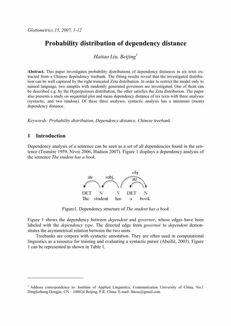
Dependency analysis of a sentence can be seen as a set of all dependencies found in the sen-tence (Tesnière 1959, Nivre 2006, Hudson 2007). Figure 1 displays a dependency analysis of the sentence The student has a book.
Figure1. Dependency structure of The student has a book Figure 1 shows the dependency between dependent and governor, whose edges have been labeled with the dependency type. The directed edge from governor to dependent demon-strates the asymmetrical relation between the two units.
Treebanks are corpora with syntactic annotation. They are often used in computational linguistics as a resource for training and evaluating a syntactic parser (Abeillé, 2003). Figure 1 can be represented as shown in Table 1.
1 Address correspondence to: Institute of Applied Linguistics, Communication University of China, No.1 Dingfuzhung Dongjie, CN – 100024 Beijing, P.R. China. E-mail: [email protected]

Haitao Liu 2
Table 1 Annotation of The student has a book in a dependency treebank
Dependent Governor
Order number
Character POS Order
number Character POS
Dependency type
1 The det 2 student n atr
2 student n 3 has v subj
3 has v
4 a det 5 book n atr
5 book n 3 has v obj
Dependency distance is the linear distance between governor and dependent (Hudson 1995). The concept was first used in Heringer/Strecker/Wimmer (1980:187). Formally, let W1...Wi...Wn be a word string. For any dependency relation between the words Wa and Wb, a, b are order numbers of the words Wa and Wb (1 ≤ a ≤ n, 1 ≤ b ≤ n, a ≠ b); if Wa is governor and Wb is dependent, then the dependency distance (DD) between them can be defined as the absolute value of the difference a-b; by this measure, adjacent words have a DD of 1. For instance, a series of dependency distances can be obtained from the sentence in Table 1 and Figure 1 as follows: 1 1 1 2. In other words, the example has three dependencies with DD = 1 and one dependency with DD = 2. Using the same method, we can also extract a series of dependency distances from a text.
Formula (1) can also be used to calculate the mean dependency distance of a larger collection of sentences, such as a text:
1
1 |n s
ii
DD DDn s
−
=
=− ∑ | (1)
In this case, n is the total number of words in the text, s is the total number of sentences in the text. DDi is the dependency distance of the i-th syntactic link of the text.
This paper will investigate the probability distribution of dependency distances of six texts, taken from a Chinese treebank. To better position the distribution found, we also compare the results with two samples of dependency treebanks with randomly generated governors.
In the next section, the frequency distribution of dependency distances based on the treebank and their fitting, using the software package Altmann-Fitter (1994/2005), are presented. Section 3 lists several results of dependency distance analyses of the six texts in question, but with randomly generated governors. Section 4 shows the result of a sequential plot and mean dependency distances of the texts. Section 5 presents concluding remarks and directions for further work.

Probability Distributions of Dependency Distance 3
2 Distributions of Dependency distances
The Chinese dependency treebank used here is based on the news (xinwen lianbo) of China Central Television, a genre which is intended to be spoken but whose style is similar to written language. The treebank includes 711 sentences and 17,809 word tokens; the mean sentence length is 25 words. To maintain text homogeneity, we have randomly extracted six texts from the treebank. Each reports on a relatively independent event.
Since distance can be measured in different ways, and we wish to keep the result more general, we derive the model of distance distribution in a continuous way. We start from the simple assumption that the relative rate of change of frequency (f(x)) is negatively proportional to the relative rate of change of distance (x), i.e.
(1) ( )( )
df x a dxf x x
= − .
Solving this simple differential equation, used very frequently in linguistics, we obtain
(2) ( ) a
Kf xx
= .
Since we measured the distance discretely and texts are finite, we transform (2) into a discrete distribution and compute the normalizing constant K, i.e. we set
(3) , 1,2,...,x a
KP xx
= = R
where R is the point of right truncation. We define the function
1
( , , )( )
j
aj
bb c ac j
∞
=
Φ =+∑
and since in (3) we have b = 1, c = 0, and the greatest distance is R, we obtain by simple subtraction the result K = [Φ(1,0,a)-Φ(1,R,a)]-1. Hence, finally we obtain
(4) 1 , 1,2,...,
[ (1,0, ) (1, , )]x aP xx a R a
= =Φ −Φ
R
representing the right truncated Zeta distribution (or Zipf distribution). The normalizing
constant can be simply written as the sum 1
1
Ra
jK j− −
=
= ∑ .
We extract from the treebank six texts and calculate the frequency of dependency distance of all dependences in texts. Then we use the software Altmann-Fitter to fit the right truncated Zeta distribution to the observed data. The results for the six texts are shown in Table 2. Hence, the hypothesis is considered as compatible with the data.

Haitao Liu 4
Table 2 Fitting the right truncated Zeta distribution to the dependency distances in six texts
No. X² DF P a R N 001 22.72 18 0.202 1.625 21 389 002 32.50 24 0.115 1.561 28 385 003 22.26 23 0.505 1.602 37 233 004 22.69 17 0.160 1.631 20 346 005 24.57 21 0.266 1.650 27 361 006 15.30 18 0.641 1.634 23 295
No – ordinal number of the texts; X2 – Chi-square; DF – degrees of freedom; P – probability of Chi-square; a, R – parameters of the right truncated Zeta distribution; N – number of the word tokens in the text.
It would be preferable to list complete results for all six texts, but to save space, we only give an example from the six texts as an illustration of the program’s output.
Table 3 Fitting the right truncated Zeta distribution to
the dependency distances in text 006
Distance x Frequency NPx 1 143 144.50 2 43 46.57 3 29 24.01 4 6 15.01 5 17 10.43 6 7 7.74 7 7 6.02 8 4 4.84 9 5 3.99 10 5 3.36 11 4 2.88 12 3 2.50 13 1 2.19 14 1 1.94 15 1 1.73 16 2 1.56 17 2 1.41 18 1 1.29 19 2 1.18 20 2 1.08 21 0 1.00 22 1 0.97 23 1 0.86
a = 1.6335, R = 23, X2 = 15.30, DF = 18, P = 0.64

Probability Distributions of Dependency Distance 5
Figure 2. Fitting the right truncated Zeta distribution to the dependency distances in text 006.
3 Distribution of dependency distances in two random treebanks Section 2 corroborates the adequateness of the right truncated Zeta distribution for the dis-tribution of dependency distances. The following questions arise: What role does syntax play in such a distribution? If we form dependencies by randomly linking words in the same texts, would the distribution still follow the right truncated Zeta distribution? In other words, are our hypotheses in section 2 characteristic of syntactic dependency structures or is the Zeta distribution a general property of a word net?
To answer these questions we construct two randomly generated versions of a segment of the treebank for the same six texts. Ideally, we could produce a language with a randomly generated lexicon and sentences, but it is difficult or impossible to syntactically analyze such a language. Therefore, by randomly assigning the governor for all words in a dependency analysis of a text, we can build a random dependency version as a sample of a random language with dependency analysis. We use two methods to generate two random dependency samples.
.
Figure 3. A possible random analysis of The student has a book with crossing arcs
In the first random analysis (RL1), disregarding syntax and meaning, within each sen-tence we select one word as root, and then, for each other word, randomly select another word in the same sentence as its governor. In this way, we can generate a possible random analysis of the sentence in Figure 3.

Haitao Liu 6
In the second random analysis (RL2), while the governor is assigned to a word, only dependency trees are generated which are projective and connected graphs, i.e. without crossing edges. Nivre (2006: 53) gives a formal definition of projectivity, which was first discussed by Lecerf (1964) and Hays (1964). Figure 4 is such a possible random analysis of the sentence in Figure 1.
Figure 4. A possible random analysis of The student has a book without crossing edges
3.1 Distribution of dependency distances in random analysis RL1
After randomly assigning the governors for all words in six texts, we calculate the dependency distances of the six texts and use the Altmann-Fitter to find a possible empirical model, because there is as yet no theoretical assumption from which we could start. It is noteworthy that the distributions do not agree any more with the right truncated Zeta distribution, as could be expected. Instead, we found that randomly generated structures are best characterized by a different distribution: The Altmann-Fitter shows that the Hyperpoisson distribution, for instance, is a good model for all six texts with randomly generated governors. The Hyperpoisson distribution is defined as
(5) ( )1 1
, 0,1,2(1; ; )
x
x x
aP xb F b a
= = ...
where b(x) = b(b+1)…(b+x-1) and 1F1(.) is the confluent hypergeometric function. We used here the 1-displaced version without truncation at the right hand side. In Table 4, the results of fitting are presented. However, in Table 5 and Figure 5, one can see the massive irregularity of the observed data. The distribution is not even monotonously decreasing; hence another model – even displaying a greater chi-square – would be more adequate, e.g. the negative binomial capturing the bell shape at the beginning of the data. But since the negative binomial has the geometric as its special case and the Hyperpoisson converges to the geometric when a → ∞, b → ∞ and a/b → q, we can save one parameter if we choose the geometric distribution. Even in that case, we still obtain a chi-square with P = 0.30
Table 4 Fitting the Hyperpoisson distribution to the dependency distances in six texts (RL1)
No. X² DF P N a b 001 39.99 41 0.515 52 1121.21 1204.19 002 44.31 58 0.907 75 787.60 802.59 003 38.69 39 0.484 49 705.72 741.09 004 32.48 36 0.637 44 881.37 956.53 005 26.32 37 0.904 48 367.02 368.77 006 39.28 56 0.956 56 7193.47 7612.17

Probability Distributions of Dependency Distance 7
Table 5 Fitting the Hyperpoisson distribution
to the dependency distances in text 002 (RL1)
X[i] F[i] NP[i] X[i] F[i] NP[i] 1 13 15.32 39 4 3.16 2 17 15.03 40 2 2.96 3 17 14.73 41 3 2.77 4 16 14.42 42 2 2.59 5 16 14.10 43 2 2.42 6 17 13.77 44 1 2.25 7 12 13.43 45 1 2.10 8 14 13.08 46 1 1.95 9 10 12.72 47 0 1.81 10 15 12.36 48 2 1.68 11 10 12.00 49 3 1.56 12 9 11.63 50 1 1.45 13 10 11.26 51 2 1.34 14 13 10.88 52 0 1.24 15 9 10.51 53 1 1.14 16 8 10.14 54 0 1.05 17 8 9.77 55 0 0.97 18 3 9.40 56 0 0.89 19 10 9.03 57 0 0.82 20 5 8.67 58 2 0.75 21 11 8.31 59 0 0.69 22 15 7.95 60 0 0.63 23 6 7.61 61 0 0.57 24 8 7.27 62 0 0.52 25 4 6.93 63 0 0.48 26 6 6.60 64 2 0.44 27 8 6.29 65 0 0.40 28 6 5.97 66 3 0.36 29 9 5.67 67 0 0.33 30 6 5.38 68 0 0.30 31 5 5.09 69 0 0.27 32 6 4.82 70 0 0.24 33 6 4.55 71 0 0.22 34 8 4.30 72 0 0.20 35 2 4.05 73 1 0.18 36 4 3.81 74 1 0.16 37 4 3.58 75 1 1.32 38 5 3.37

Haitao Liu 8
Figure 5. Fitting the Hyperpoisson distribution to the dependency distances in text 002 (RL1). Table 4 shows that the distribution of the dependency distances of six texts with randomly generated governors abide by the Hyperpoisson distribution, but a number of other distribu-tions would be adequate, too. However, the observed data displayed in Figure 5 do not comply with the linguistic expectation of an “honest” distribution.
3.2 Distribution of the dependency distances in random analysis RL2
Obviously, the dependency graph generated by the above-mentioned method is not syntactic. Projectivity is a feature of most dependency graphs (trees) of natural language, although there are non-projective structures in some languages. Therefore, to find the influence of project-ivity on the distribution of dependency distances, we add the constraint of projectivity (no crossing edges) when generating randomly the governor of a dependency graph.
In this subsection, we present the result of fitting the right truncated Zeta to dependency distance in RL2.
Table 6
Fitting the right truncated Zeta distribution to the dependency distances in six texts (RL2)
No. X² DF P a R 001 21.92 38 0.983 1.389 48 002 38.06 45 0.759 1.394 65 003 31.29 30 0.401 1.408 46 004 29.83 34 0.672 1.388 43 005 25.44 33 0.824 1.334 36 006 29.70 36 0.761 1.388 52

Probability Distributions of Dependency Distance 9
Table 7 Fitting the right truncated Zeta distribution to dependency distance in text 003 (RL2)
X[i] F[i] NP[i] X[i] F[i] NP[i]
1 84 88.36 24 0 1.01 2 36 33.31 25 2 0.95 3 32 18.82 26 1 0.90 4 17 12.55 27 1 0.85 5 7 9.17 28 1 0.81 6 6 7.09 29 0 0.77 7 1 5.71 30 1 0.74 8 3 4.73 31 1 0.70 9 3 4.01 32 0 0.67 10 3 3.46 33 0 0.64 11 4 3.02 34 0 0.62 12 2 2.67 35 0 0.59 13 3 2.39 36 0 0.57 14 2 2.15 37 0 0.55 15 2 1.95 38 0 0.58 16 3 1.78 39 0 0.51 17 0 1.68 40 0 0.49 18 2 1.51 41 0 0.47 19 0 1.40 42 0 0.46 20 1 1.30 43 1 0.44 21 2 1.22 44 1 0.43 22 1 1.14 45 1 0.42 23 0 1.07 46 1 0.40
Figure 6. Fitting the right truncated Zeta distribution to dependency distance in text 003 (RL2)

Haitao Liu 10
It is interesting to note that the results have the same good agreement with the right truncated Zeta distribution as natural language. Evidently, projectivity is the background mechanism of this phenomenon.
4 Sequential plot and mean dependency distance
The results in section 3 show that the distribution of dependency distances may not be a sufficient or unique criterion to distinguish syntactic and non-syntactic data. Ferrer i Cancho (2006) suggests that the uncommonness of crossings in the dependency graph could be a side-effect of minimizing the Euclidean distance between syntactically related words. In other words, perhaps we have to investigate the mean dependency distance of a text in three manners (syntactic, RL1 and RL2).
To compare the distribution of dependency distances in three samples, we use sequential plots of dependency distances for text 1 in three analyses (syntactic, RL1 and RL2) as shown in Figure 7.
Figure 7 shows that dependency distance in RL1 has the greatest fluctuant range, the con-straint “no-crossing edges” decreases the range in RL2, and the role of syntax is also obvious in minimizing dependency distances of a sentence or text. The comparison of pictures in Figure 7 shows that in NL (syntactic) texts there is still another mechanism (besides project-ivity) rendering the sequence of distances almost homogeneous; while RL2 arising randomly has a much greater fractal dimension and the oscillation could, perhaps be captured by a very complex Fourier analysis. But no generalization is possible before other languages have been analyzed.
Using formula (1), we can obtain the mean dependency distance of six texts in three manners. The results are shown in Table 9.
Figure 7. Sequential plots of text 001. Above: syntactic (NL); Middle: RL1; Below: RL2.

Probability Distributions of Dependency Distance 11
Table 9 Mean dependency distances of six texts
Text NL RL1 RL2 1 2.971 12.040 5.421 2 3.427 18.575 5.925 3 3.636 12.693 5.253 4 3.027 10.015 4.834 5 3.360 11.209 4.969 6 3.387 17.080 5.770
MDD 3.3 13.6 5.4 Figure 8 shows diagrammatically the change of the range and the distribution of mean dependency distances in 6 texts.
Figure 8: Distribution of mean dependency distance in NL, RL1 and RL2
Our experiments show that projectivity can restrict the dependency distances (Ferrer i Cancho 2006), because RL2 has a lower mean DD than RL1. However, it is also noteworthy that we cannot explain why natural language has a minimized mean DD from this point of view only. Figure 8 demonstrates that natural language has a smaller mean DD than RL2. That suggests that syntax also plays a certain role in minimizing the mean DD of a language. Figure 8 provides a functional view of syntactic word-order restrictions: one of their (many) benefits is the reduction of the mean DD of a sentence or text. It seems that projectivity and syntax co-operate to allow us to use long sentences, but keep the mean DD within an acceptable range.
5 Conclusions
We have investigated the probability distributions of dependency distances in six texts extracted from a Chinese dependency treebank. The results reveal that the data can be well captured by the right truncated Zeta distribution. To see whether the conclusion holds only for a natural language, we constructed two samples with randomly generated governors, but with the same texts. The most random one needs the addition of a further parameter, the other one abides by the right truncated Zeta distribution. The paper also presents a study on sequential plots and mean dependency distances of six texts with three analyses (a syntactic and two random ones). The results show that syntax plays an important role in minimizing the (mean) dependency distance and in turn for the minimization of decoding effort. The shorter the

Haitao Liu 12
dependency distances, the smaller is the decoding effort of the sentence (Gibson 2000). Thus, the problem has its psycholinguistic and synergetic counterparts.
Considering the importance of dependency distance for any linguistic applications based on the dependency principle, the study contributes to a quantitative understanding of dependency syntax. Further research in projectivity is needed to investigate why RL2 abides by the same regularity as a natural text, while it has a greater mean DD than a natural (syntactic) text.
Acknowledgements
We thank Gabriel Altmann, Richard Hudson and Reinhard Köhler for insightful discussions, Hu Fengguo for generating random dependency samples, Zhao Yiyi for annotating the treebank.
References
Abeillé, A. (ed). (2003). Treebank: Building and using Parsed Corpora. Dordrecht: Kluwer. Ferrer i Cancho, Ramon (2006). Why do syntactic links not cross? Europhysics Letters 76
1228-1235. Gibson, E. (2000). The dependency locality theory: a distance-based theory of linguistic
complexity. In: Marantz, A. et. al. (eds), Image, language, brain (P. 95-126). Cam-bridge, MA: The MIT Press.
Hays, David G. (1964). Dependency Theory: A Formalism and Some Observations. Lan-guage 40: 511-525.
Heringer, H. J., Strecker, B., & Wimmer, R. (1980). Syntax: Fragen-Lösungen-Alter-nativen. München: Wilhelm Fink Verlag.
Hudson, R. A. (1995). Measuring Syntactic Difficulty. Unpublished paper. http://www.phon.ucl.ac.uk/home/dick/difficulty.htm (2007-6-6)
Hudson, R.A. (2007). Language Networks: The New Word Grammar. Oxford: Oxford University Press.
Lecerf, Y. (1960). Programme des conflits-modèle desconflits. Rapport CETIS. No. 4, Euratom. p. 1-24.
Nivre, J. (2006). Inductive Dependency Parsing. Dordrecht: Springer. Tesnière, L. (1959) Eléments de la syntaxe structurale. Paris: Klincksieck.
Software
Altmann-Fitter (1994/2005). Iterative Fitting of Probability Distributions. Lüdenscheid: RAM-Verlag.

Glottometrics 15, 2007, 13-23
Russizismen im deutschen Wortschatz
Oxana Kotsyuba, Dortmund1
Abstract. The history of the German language is a history depicting the influence of foreign lan-guages on German, as has been portrayed in different publications on the influence of the English, French, and Italian languages. The influence of other modern languages, among them the Russian lan-guage, has not been analysed to a great extent. This paper, based on gained data, intends to determine whether the Piotrowski-Law applies to the process of word-borrowing from Russian into German. Keywords: Borrowings, German, Russian, Piotrowski-law Das Piotrowski-Gesetz als Modell für Entlehnungsprozesse
Der vorliegende Beitrag ist einer weiteren Bestätigung eines Sprachgesetzes, in diesem Fall des Piotrowski-Gesetzes, gewidmet. Es wurde am Beispiel der Übernahme von Russizismen in die deutsche Sprache erneut erprobt. Um dies durchzuführen, wurde eigens für diese Unter-suchung ein neues Korpus erarbeitet.
Im Folgenden wird zunächst das Prinzip des Piotrowski-Gesetzes dargestellt. ”Unter dem Piotrowski-Gesetz verstehen wir die hypothetische Aussage über den zeitlichen Verlauf der Veränderungen einer beliebigen sprachlichen Entität” (Altmann 1983:59). Das Gesetz ist nach dem sowjetischen Linguisten Raimond Genrichowitsch Piotrowski benannt. Dieses lo-gistische Gesetz ist auf verschiedene Formen des Sprachwandels anwendbar, wobei unter Sprachwandel der Veränderungsprozess von Sprachelementen und Sprachsystemen in der Zeit verstanden wird. Es lassen sich drei unterschiedliche Formen des Sprachwandels unter-scheiden:
• der vollständige Sprachwandel, bei dem alte Formen vollständig durch die neuen For-men ersetzt werden (z.B. was zu war);
• der unvollständige Sprachwandel, bei dem sich die neuen Formen und Wörter nur in einem begrenztem Maß durchsetzen (z.B. Fremdwörter);
• der reversible Sprachwandel, bei dem neue Formen und Wörter aufkommen, sich ausbreiten und dann wieder verschwinden (z.B. die e-Epithese im Deutschen).
Bei Entlehnungen wird der schon vorhandene Wortschatz einer Sprache ergänzt oder auch teilweise ersetzt, aber nie ganz verdrängt. Also handelt es sich dabei um den Typ einer un-vollständigen Sprachänderung. Dafür wurde folgende mathematische Funktion entwickelt:
(1) btt aecp −+
=1
(zur Begründung und Ableitung des Modells vgl. Altmann 1983: 60f, Formel 7). Es handelt
1 Address correspondence to: [email protected]

Oxana Kotsyuba 14
sich dabei um ein Wachstumsmodell vom logistischen Typ, wie es in der Biologie, Sozio-logie, Ökonomie oder in der Bevölkerungsdynamik seit langem Anwendung findet.
Das Piotrowski-Gesetz beschreibt allgemein den zeitlichen Verlauf der Veränderung sprachlicher Einheiten. Mithilfe dieses Gesetzes ist es möglich vorauszusagen, wie ein begon-nener Sprachwandel weiter verläuft. Eine sehr wichtige Voraussetzung ist, dass sich die Bedingungen, unter denen dieser Sprachwandel stattgefunden hat, nicht wesentlich verändern, sondern gleich bleiben.
Eine modellhafte Erprobung und Überprüfung des Piotrowski-Gesetzes findet sich in vielen empirischen Untersuchungen zum Sprachwandel im Deutschen. Die Annahme, dass die Entlehnungsprozesse tatsächlich dem oben genannten Modell entsprechen, konnte für Ent-lehnungen aus Latein, Französisch, Niederdeutsch, Niederländisch, Italienisch, Spanisch, Griechisch und weitere Sprachen bestätigt werden (vgl. Best & Altmann 1986). Später sind die gewonnenen Ergebnisse von Best (2001b) anhand einer weiteren Datenbasis überprüft worden und das Modell hat sich auch dabei bewährt. Der Einfluss der Sprachen, von denen das Deutsche über Jahrhunderte hinweg immer wieder Wörter entlehnt hat, ließ die Sprach-wandelprozesse in diesen Untersuchungen den typischen S-förmigen Verlauf nehmen.
Auch der englische Einfluss auf das Deutsche wurde untersucht und konnte anhand des Piotrowski-Gesetzes nachvollzogen werden (vgl. Best & Altmann 1986; Best 2001b, 2003b; Körner 2004).
Der Zuwachs der deutschen, lateinischen und slawischen Wörter im Ungarischen wurde in der Arbeit von Beöthy & Altmann (1982) erforscht und die Gesetzmäßigkeit des Verlaufs von Entlehnungsprozessen wurde anhand des Piotrowski-Gesetzes erneut bestätigt.
Im Artikel von Helle Körner (2004) wird das logistische Gesetz unter anderem anhand der Datenbasis der slawischen Wörter überprüft. Das Korpus enthält 44 Slawismen. Die Autorin fasst sämtliche slawischen Sprachen, aus denen Wörter übernommen worden sind, unter dem Sammelbegriff Slawisch zusammen, um eine Datenauswertung zu ermöglichen. Andernfalls wären für jede einzelne dieser Sprachen zu wenige Belege vorhanden gewesen (vgl. Körner 2004:40). Entlehnungen aus dem Russischen sind nicht gesondert betrachtet worden.
In Bezug auf den slawischen bzw. russischen Einfluss im Deutschen ist die Arbeit von Karl-Heinz Best (2003a) nennenswert. Der Autor führt zwei Auswertungsverfahren durch. Zum einen wird der Prozess der Übernahme slawischer Wörter insgesamt anhand des Piot-rowski-Gesetzes unter Beweis gestellt. Zum anderen wird die Gesetzmäßigkeit des Verlaufs von Entlehnungen aus dem Russischen überprüft. Für die übrigen slawischen Sprachen stehen nicht genügend Daten zur Verfügung. Die Datenbasis dieser Untersuchung enthält 124 sla-wische Entlehnungen, darunter 56 Lehnwörter aus dem Russischen. Bei der Auswertung der Daten stößt Best auf das Problem der auffallend hohen Zunahme slawischer Lehnwörter im 20. Jahrhundert, für die ausnahmslos der russische Einfluss verantwortlich ist. Für die späte-ren Untersuchungen schlägt der Autor vor, von den Lehnwörtern des 20. Jahrhunderts dieje-nigen zu streichen, die unter politischem bzw. ideologischem Einfluss entstanden. Diese Lehnwörter würden aufgrund der politischen Entwicklung in Deutschland und in Osteuropa in den 1990er Jahren nur noch relativ kurze Zeit eine Rolle in der deutschen Sprache spielen (vgl. Best 2003a: 469).
Beide Autoren, Körner und Best, weisen darauf hin, dass die Korpora für slawische bzw. russische Entlehnungen erweitert werden sollten, damit die Ergebnisse der Untersuchungen als zuverlässiger und repräsentativer angesehen werden könnten. Außer diesen zwei erwähn-ten Arbeiten sind anscheinend keine anderen Untersuchungen zur Gesetzmäßigkeit des Ver-laufs der Entlehnungsprozesse aus den slawischen Sprachen bzw. aus dem Russischen vorhanden. Es gibt also hinreichend Gründe dafür, zu versuchen, die Datenbasis zu erweitern

Russizismen im deutschen Wortschatz 15
und danach die Gültigkeit des Piotrowski-Gesetzes erneut zu prüfen. Dieses Ziel verfolgt die vorliegende Untersuchung.
Methodik der Untersuchung Bei der Durchführung der vorliegenden Untersuchung werden folgende methodische Aspekte berücksichtigt:
• das lexikographische Fundament des Korpus; • qualitative Bestandteile der Datenbasis; • Behandlung von Problemen bei Zeitangaben; • Behandlung von Problemen bei der Vermittlersprache.
Im Folgenden werde ich auf einzelne Aspekte der Methodik näher eingehen, um den Prozess des Zusammenstellens des Korpus darzustellen. Das lexikographische Fundament des Korpus Das Untersuchungskorpus für die vorliegende Untersuchung wurde mithilfe der lexiko-graphischen Analyse verschiedener Fremdwörterbücher und Fachbücher zusammengestellt. Als Ausgangspunkt für die Zusammenstellung des Korpus dienten folgende Untersuchungen:
• die Dissertation Russisches lexikalisches Lehngut im deutschen Wortschatz von Siegfried Kohls (1964)
• die Untersuchung Ostslawische lexikalische Elemente im Deutschen von Efim Opel’baum (1971)
• eine alphabetische Zusammenstellung der im Deutschen verwendeten Wörter aus slawischen und anderen Sprachen von Klaus Müller aus dessen Buch Slawisches im deutschen Wortschatz (1995).
Die lexikographische Fixierung entlehnter russischer Wörter und die Vervollständigung des Korpus wurden im Weiteren durch folgende Quellen ergänzt und erweitert:
• das Etymologische Wörterbuch der deutschen Sprache von Friedrich Kluge (1999) • das Etymologische Wörterbuch des Deutschen von Wolfgang Pfeifer (1993) • die Auswertung der Brockhaus Enzyklopädie (1989).
Russische Entlehnungen wurden auch in den Arbeiten von Hans Holm Bielfeldt (1963; 1965; 1982) und im Altrussischen Lexikon von Erich Donnert (1988) untersucht. Aus diesen Werken sind ebenfalls Entlehnungen in mein Korpus eingeflossen. Qualitative Bestandteile der Datenbasis Die Basis für die vorliegende Untersuchung bilden 262 Entlehnungen aus dem Russischen. Das Korpus enthält ausschließlich die Übernahmen aus dem Russischen in den deutschen Wortschatz. Zu dem zu untersuchenden lexikalischen Lehngut gehören assimilierte und nicht assimilierte Lehnwörter russischer Herkunft sowie russischer Vermittlung.
Russische geographische Bezeichnungen (z.B. Wolga), Personennamen (z.B. Iwan), Ei-gennamen (z.B. Aeroflot), spezielle russische Fachausdrücke und nur gelegentlich belegte russische Wörter wie auch phraseologische Redewendungen sind nicht berücksichtigt worden.
Was das entlehnte Wortgut des 20. Jahrhunderts angeht, so enthält die Datenbasis einige
Oxana Kotsyuba 16
Sowjetismen, die im politischen Wortschatz eine Rolle spielten bzw. spielen (von Bolschewik, Kolchos(e), Komsomol, Kulak, Sowjet bis hin zu Glasnost und Perestrojka aus den 1980er Jahren). Bildungen aus Eigennamen werden nur ausnahmsweise aufgenommen (z.B. Stali-nismus, Trotzkismus usw.). Die große Zahl weiterer Ableitungen (z.B. Bykow-Methode, Hon-necke-Bewegung, Lenin-Preis usw.) bleibt unberücksichtigt.
Die Lehnprägungen, darunter vor allem Lehnübersetzungen und Lehnbedeutungen, die den russischen Einfluss zur DDR-Zeit geprägt haben, sind in Anlehnung an Best (2003a) aus zwei Gründen nicht in die Datenbasis übernommen worden. Zum einen, da diese Wörter nur auf dem DDR-Territorium verbreitet waren und in der Bundesrepublik entweder gar nicht bekannt waren oder nur selten benutzt wurden. Zum anderen wird ein erheblicher Teil dieses Wortschatzes im Deutschen keine Zukunft mehr haben, da er bereits in Vergessenheit geraten ist (vgl. Hellmann 1990: 267).
Ableitungen wie kolchosieren oder jarowiesieren sowie umgangssprachliche Lehnwörter (dawaj, nitschewo, pascholl, stupaj, stoj), die meistens als Okkasionalismen verwendet wer-den, werden nicht in die Datenbasis übernommen. Die Behandlung von Problemen bei Zeitangaben Die untersuchten Wörter sind zu verschiedenen Zeitpunkten in den deutschen Wortschatz eingegangen. Für eine systematische Auswertung des Korpus sind die genauen Angaben über das Jahrhundert der Übernahme notwendig.
In die Datenbasis wurden nur die Lehnwörter übernommen, bei denen das Jahrhundert der Übernahme ausreichend genau bestimmbar ist. Die Zeit der Übernahme wird in der Regel aufgrund der Erstbelege im Deutschen nach dem derzeitigen Forschungsstand beschrieben. An dieser Stelle muss ausdrücklich darauf hinwiesen werden, dass nicht alle Forscher das Datum der Übernahme der in meinem Korpus angeführten Wörter gleich bestimmen. Zum Feststellen der Datierbarkeit wurden insgesamt drei Untersuchungen von Opel’baum (1971), Kohls (1964) und Müller (1995) herangezogen. Wenn die Angaben in den ersten beiden Fachbüchern eine eindeutige Zuordnung zu einem Jahrhundert aufwiesen und übereinstimmten, wurden diese Angaben ohne nochmalige Überprüfung durch andere Fach- und Wörterbücher übernommen. Wenn aber Unstimmigkeiten auftraten, wurden das Buch von Klaus Müller sowie die Wörterbücher von Kluge (1999) und Pfeiffer (1993) hinzugezogen. Wenn zwei der drei verwendeten Fach- oder Wörterbücher Übereinstimmungen zeigten, wurde diese Datierung als eindeutige Angabe gewertet. Wenn aber Widersprüche und Abweichungen auftraten, wurde das Lehnwort aus der Datenbasis ausgeschlossen.
In Anlehnung an Best (2001a) sind die Entlehnungen, die zwei Jahrhunderten zugeordnet sind, wie z.B. ”16./17. Jahrhundert”, dem erstgenannten Zeitraum zugerechnet worden. Die Angaben ”um 1700” werden dem folgenden, 18. Jahrhundert zugewiesen (vgl. Best 2001a:8). Bei Wörtern, die aus anderen Sprachen über das Russische vermittelt wurden, wird nur die Zeitangabe des Übergangs ins Deutsche angegeben. Undatierte Entlehnungen wurden nicht berücksichtigt.
Die Lehnwörter im Korpus werden im Allgemeinen Jahrhunderten zugewiesen (z.B. 17. Jh.; 1. Hälfte 18. Jh.; Mitte 19. Jh.; 2. Hälfte 20. Jh.). Die Behandlung von Problemen bei der Vermittlersprache Für die Auswertung etymologischer Wörterbücher gibt es zwei Herangehensweisen: Ent-weder wird die Vermittlersprache, d.h. die Sprache, über die ein Wort ins Deutsche gelangt ist, berücksichtigt, oder aber die Herkunftssprache, d.h. die Sprache, aus der ein Wort ur-

Russizismen im deutschen Wortschatz 17
sprünglich stammt. Je nach Verfahren ergeben sich also andere Zuordnungen. In Anlehnung an Best (2001a: 8) war für diese Auswertung lediglich die Vermittlersprache ausschlag-gebend.
Einige Lehnwörter, die bei Siegfried Kohls (1964) als Entlehnungen aus dem Russischen und bei Efim Opel’baum (1971) und Klaus Müller (1995) als ukrainische Entlehnungen ver-zeichnet sind, wurden nicht in die Datenbasis übernommen, z.B. Bandura, Baschtan, Basch-tanik, Borschtsch, Duma ”ukrainisches Volkslied”, Haidamaken, Hopack, Kalamaika, Kelim (Kilim), Kobsa, Kobsar, Kosak ”ukrainischer Volkstanz”, Rada und Hetman (vgl. Opel’baum 1971: 238, Müller 1995: 23).
Nicht aufgenommen wurden auch Wörter, bei denen die russische Herkunft bisher ange-nommen wurde, doch aufgrund neuer Forschungen nicht gesichert erscheint (z.B. Grippe).
Entlehnungen aus dem Englischen, die auf dem ehemaligen DDR-Territorium durch das Russische vermittelt wurden, wurden in die Datenbasis ebenfalls nicht übernommen, weil sie keine allgemeine Verbreitung in der deutschen Sprache gefunden haben und deshalb für diese Untersuchung nicht repräsentativ sind. Die Lehnwörter, die ursprünglich aus den türk-tatari-schen, mandschu-tungusischen, kaukasischen und semitischen Sprachen stammen und bei denen das Russische als Vermittlungssprache auftritt, wurden allerdings in die Datenbasis übernommen, sofern die Datierung klar war.
Aufgenommen sind weitere Wörter, die vom Russischen vermittelt sind; dabei kann es sich um eine Rückentlehnung handeln (z.B. Budka, Duma ”Ratsversammlung, Stadthaus”, Kapusta, Knute, Polk, Sterlet). Auswertung Es wird von der Annahme ausgegangen, dass der Prozess der Übernahme von Fremdwörtern ebenso wie alle anderen Sprachwandelprozesse gesetzmäßig verläuft und dabei dem soge-nannten Piotrowski-Gesetz folgt. Anhand der zur Verfügung stehenden Daten wurde geprüft, ob dies sich auch für den Einfluss der russischen Sprache auf das Deutsche nachweisen lässt. Das hier angewendete Testverfahren hat G. Altmann (1983: 74ff) beschrieben.
Für die russischen Entlehnungen kommen nach der Auszählung der zusammengestellten Datenbasis und der anschließenden Berechnung folgende Werte zustande (vgl. Tabelle 1).
Tabelle 1
Übernahme russischer Entlehnungen ins Deutsche (10.-20. Jh.)
Jahrhundert t n n (kumuliert) p (berechnet) 10. 1 1 1 0,68 11. 2 1 2 1,33 12. 3 0 2 2,59 13. 4 5 7 5,03 14. 5 4 11 9,73 15. 6 7 18 18,68 16. 7 23 41 35,27 17. 8 30 71 64,66 18. 9 21 92 112,77 19. 10 105 197 182,10 20. 11 65 262 265,73
A = 1470.5335 b = 0.6698 c = 512.4192 D = 0.99 • t gibt die Nummer der zu untersuchenden Jahrhunderte an;

Oxana Kotsyuba 18
• n gibt die Anzahl der ausgezählten Wörter für das entsprechende Jhd. an (beobachtete Werte); • n (kumuliert) gibt die Summe aller bis zum entsprechenden Jahrhundert übernommenen
Wörter an (kumulierte Werte); • p (berechnet) führt theoretisch nach der Funktion p(t) von Altmann berechnete Werte für das
entsprechende Jahrhundert auf. Die Berechnung der Daten erfolgte mithilfe des Programms NLREG Version 6.3. Eine De-monstrationsversion dieses Programms kann man im Internet von der Seite http://www.nlreg.com/ herunterladen.
• a, b und c sind Parameter des logistischen Gesetzes • c gibt den berechneten Wert für den Sprachwandel an, der anzeigt, gegen welchen
Wert der Sprachwandel strebt. Dabei ist unter c nicht ein absoluter Wert zu verstehen, der tatsächlich angibt, wie viele Wörter im Höchstfall aus der jeweiligen Sprache übernommen werden, sondern nur eine Tendenz, die je nach Datenbasis variiert;
• D ist der Determinationskoeffizient. Je größer D ist, desto besser ist die Anpassung. Es soll D ≥ 0.80 gelten, um sagen zu können, dass das Modell den Sprachwandelprozess in annehmbarer Weise wiedergibt. In unserem Fall handelt es sich um den Wert D = 0.99. Dies bedeutet eine sehr gute Anpassung.
• Diese Erklärungen gelten auch für die nächste Tabelle.
Nach Einsetzung der errechneten Parameter in die Formel (1) ergibt sich für die Übernahme der Russizismen im deutschen Wortschatz folgender Term:
tt ep 6698,05335,14701
4192,512−+
= .
Die Übernahme russischer Wörter ins Deutsche wird in der folgenden Graphik (vgl. Abb. 1) dargestellt; dabei wurde die Linie für die berechneten Werte über den Beobachtungszeitraum hinweg durchgezogen, um eine Vorstellung davon zu geben, wie die zukünftige Entwicklung sein könnte.
Abbildung 1. Übernahme russischer Wörter ins Deutsche (10. – 20. Jh.)
Die y-Achse bezeichnet die Anzahl der Wörter, auf der x-Achse wird die Zeit (in Jahrhun-derten) eingetragen. Die durchgehende Linie gibt in Übereinstimmung mit Formel 1 den Ver-
Russizismen im deutschen Wortschatz 19
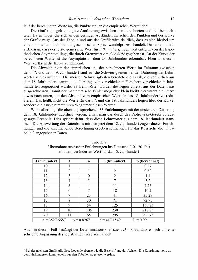
lauf der berechneten Werte an, die Punkte stellen die empirischen Werte2 dar. Die Grafik spiegelt eine gute Annäherung zwischen den berechneten und den beobach-
teten Daten wider, die sich an den geringen Abständen zwischen den Punkten und der Kurve der Grafik zeigt. Aus der Tabelle und aus der Grafik wird deutlich, dass es sich hierbei um einen momentan noch nicht abgeschlossenen Sprachwandelprozess handelt. Das erkennt man z.B. daran, dass der letzte gemessene Wert für n (kumuliert) noch weit entfernt von der hypo-thetischen Asymptote liegt, die durch Grenzwert c = 512,4192 gegeben ist. An der Kurve der berechneten Werte ist die Asymptote ab dem 23. Jahrhundert erkennbar. Eben ab diesem Wert verflacht die Kurve zunehmend.
Die Abweichungen der empirischen und der berechneten Werte im Zeitraum zwischen dem 17. und dem 19. Jahrhundert sind auf die Schwierigkeiten bei der Datierung der Lehn-wörter zurückzuführen. Die meisten Schwierigkeiten bereitete die Lexik, die vermutlich aus dem 18. Jahrhundert stammt, die allerdings von verschiedenen Forschern verschiedenen Jahr-hunderten zugeordnet wurde. 33 Lehnwörter wurden deswegen vorerst aus der Datenbasis ausgeschlossen. Damit der mathematische Fehler möglichst klein bleibt, verrutscht die Kurve etwas nach unten, um den Abstand zum empirischen Wert für das 18. Jahrhundert zu redu-zieren. Das heißt, nicht die Werte für das 17. und das 19. Jahrhundert liegen über der Kurve, sondern die Kurve nimmt ihren Weg unter diesen Werten.
Wenn allerdings die oben angesprochenen 33 Entlehnungen mit der unsicheren Datierung dem 18. Jahrhundert zuordnet werden, erhält man das durch das Piotrowski-Gesetz voraus-gesagte Ergebnis. Dies spricht dafür, dass diese Lehnwörter aus dem 18. Jahrhundert stam-men. Die Auswertung der Datenbasis mit den jetzt dem 18. Jahrhundert zugeordneten Entleh-nungen und die anschließende Berechnung ergeben schließlich für das Russische die in Ta-belle 2 angegebenen Daten.
Tabelle 2
Übernahme russischer Entlehnungen ins Deutsche (10.- 20. Jh.) mit dem veränderten Wert für das 18. Jahrhundert
Jahrhundert t n n (kumuliert) p (berechnet)
10. 1 1 1 0.27 11. 2 1 2 0.62 12. 3 0 2 1.4 13. 4 5 7 3.2 14. 5 4 11 7.25 15. 6 7 18 16.2 16. 7 23 41 35.29 17. 8 30 71 72.75 18. 9 54 125 135.83 19. 10 105 230 218.85 20. 11 65 295 298.73
a = 3527.6687 b = 0.8267 c = 417.1549 D = 0.99 Auch in diesem Fall bestätigt der Determinationskoeffizient D = 0.99, dass es sich um eine sehr gute Anpassung des logistischen Gesetzes handelt.
2 Bei der nächsten Grafik gilt diese Legende ebenso wie die Beschriftung der Achsen. Die Zuordnung von t zu den Jahrhunderten kann jeweils aus den Tabellen abgelesen werden.

Oxana Kotsyuba 20
Aus den errechneten Parametern und dem ermittelten Grenzwert ergibt sich für die Übernahme der Russizismen im deutschen Wortschatz folgender Term:
tp = te 8267,06687,352711549,417
−+
Die Übernahme russischer Wörter ins Deutsche stellt sich grafisch wie in Abb. 2 dargestellt dar.
Abbildung 2. Übernahme russischer Entlehnungen ins Deutsche (10.- 20. Jh.)
mit dem veränderten Wert für das 18. Jahrhundert
Die Verbesserung spiegelt sich in der Grafik deutlich wider: Die Punkte (empirische Werte) liegen wesentlich besser auf der Kurve. Betrachtet man die Grafik, so sieht man, wie die Kur-ve schon ab dem 21. Jahrhundert zunehmend verflacht und sich asymptotisch dem c-Wert nähert. Dies verweist darauf, dass bei gleichbleibenden Umständen in der Zukunft vermutlich nur eine schwache Übernahme der russischen Lehnwörter erfolgen, und der Übernahmepro-zess bald (ceteris paribus) abgeschlossen sein wird.
Die Erhöhung des Datensatzwertes für das 18. Jahrhundert bewirkt, dass die Tendenz, nach der Wörter aus dem Russischen ins Deutsche übernommen werden, nicht mehr so steil wie in der ersten Betrachtung ausfällt. Dort lag der Datenpunkt für das 18. Jahrhundert weiter von den Werten für das 19. und das 20. Jahrhundert entfernt, was eine höhere Kurvensteigung und dementsprechend ihr späteres Abflachen bedeutet. Da der Wertunterschied jetzt kleiner geworden ist, kann die Steigung geringer bleiben und die Grafikkurve früher abflachen.
In den empirischen Werten für das 19. und das 20. Jahrhundert spiegeln sich die rasanten politischen, wirtschaftlichen und wissenschaftlichen Entwicklungen des 19. und 20. Jahrhun-derts in Russland wieder. Gleichzeitig haben die politischen Veränderungen in Europa bzw. in der ehemaligen DDR und in den ehemaligen Ostblockstaaten um 1990 herum die lexika-lischen Einflüsse besonders des Russischen auf das Deutsche stark beeinflusst und wesentlich modifiziert. Der extreme Zuwachs der russischen Wörter im 19. und 20. Jahrhundert lässt sich durch den gewaltigen politischen und wirtschaftlichen Aufschwung erklären. Zu dieser Zeit kommt es zu einer wichtigen Reform – die Befreiung der Bauern von Fronen (Barschtschina) und Abgaben an die Gutsherren. Als wichtigste Quellen des neuen russischen Lehngutes blei-ben Reiseberichte sowie kommerzielle und diplomatische Urkunden. Hinzu kommen noch

Russizismen im deutschen Wortschatz 21
russische literarische Werke, die seit Anfang des 19. Jahrhunderts ins Deutsche übersetzt wur-den. Bei den Entlehnungen aus dem 20. Jahrhundert handelt es sich um einen Wortschatz, der auf die politische und ideologische Dominanz der Sowjetunion in Osteuropa zurückzuführen ist. Ergebnis Das logistische Gesetz in der unvollständigen Form konnte mit einem sehr guten Ergebnis an beiden Datensätzen bestätigt werden. Dies unterstützt die theoretischen Annahmen zu di-versen Sprachwandelprozessen. Problematisch ist dabei die Betrachtung des Grenzwertes c. Zur Schwierigkeit der Interpretation des Grenzwertes c sagt Karl-Heinz Best:
”Es spricht daher tatsächlich alles dagegen, die Schätzwerte für c als genaue Werte für den Zuwachs zu verstehen. Sie sind rechnerische Größen, die sich ergeben, wenn man untersucht, ob die Formel für den unvollständigen Sprach-wandel ein geeignetes Modell für die jeweilige Datenbasis darstellt. Wenn c interpretiert werden soll, so immer nur bezogen auf die Wörterbücher, die die Daten für den Entlehnungsprozess geliefert haben. Ein Schluss auf das Lexikon der Sprache insgesamt ist nur denkbar, wenn man berücksichtigt, dass jedes Wörterbuch einen unterschiedlichen Ausschnitt aus dem Vokabular der Sprache darbietet und wenn man diesem Wörterbuch eine gewisse Repräsentativität für die Sprache zubilligen kann.” (Best 2001c: 14)
Der Wert c gibt also an, gegen welchen Zielwert der Entlehnungsprozess strebt. Dieser Wert wird nur als Prognose für den betrachteten Prozess gewertet.
Die vorliegende Untersuchung zur Gesetzmäßigkeit des Verlaufs von Entlehnungspro-zessen kann für den russischen Einfluss auf das Deutsche als durchaus repräsentativ gelten. In beiden Fällen konnte der typische S-förmige Verlauf eines unvollständigen Sprachwandel-prozesses bzw. der Fremdwortübernahme in der Sprache beobachtet werden, wie dies bereits unter anderem von Best & Altmann (1986), Best (2001a, 2001b, 2003a, 2003b) gezeigt wurde. Das logistische Gesetz wird somit auch in seiner Anwendung auf Entlehnungen aus dem Russischen bestätigt. Die durchgeführte Untersuchung gibt nicht nur einen rein histo-rischen Überblick, sondern auch die Möglichkeit, sich einen Ausblick auf potentielle Weiter-entwicklungen einzelner Entlehnungsprozesse – in diesem Fall über den Entlehnungsprozess aus dem Russischen – zu verschaffen.
Literatur Altmann, Gabriel (1983): Das Piotrowski-Gesetz und seine Verallgemeinerungen. In: Best,
Karl-Heinz, & Kohlhase, Jörg (Hrsg.), Exakte Sprachwandelforschung: 59-90. Göt-tingen: edition herodot.
Beöthy, Erzsébet, & Altmann, Gabriel (1982): Das Piotrowski-Gesetz und der Lehn-wortschatz. Zeitschrift für Sprachwissenschaft 1, 171-178.
Best, Karl-Heinz (1999). Quantitative Linguistik: Entwicklung, Stand und Perspektive. Göttinger Beiträge zur Sprachwissenschaft 2, 7-23.
Best, Karl-Heinz (2001c). Der Zuwachs der Wörter auf –ical im Deutschen. Glottometrics 2, 11-16.

Oxana Kotsyuba 22
Best, Karl-Heinz (2001a). Wo kommen die deutschen Fremdwörter her? Göttinger Beiträge zur Sprachwissenschaft 5, 7-20.
Best, Karl-Heinz (2001b). Ein Beitrag zur Fremdwortdiskussion. In: von Stefan J. Schierholz u.a. (Hrsg.), Die deutsche Sprache in der Gegenwart. Festschrift für Dieter Cherubim zum 60. Geburtstag: 263-270. Frankfurt/ M: Verlag Peter Lang.
Best, Karl-Heinz (2003a). Slawische Entlehnungen im Deutschen. In: Sebastian Kempgen, Ulrich Schweier und Tilman Berger (Hrsg.), Rusistika-Slavistika-Lingvistika. Fest-schrift für Werner Lehfeldt zum 60. Geburtstag: 464-473. München: Verlag Otto Sag-ner.
Best, Karl-Heinz (2003b). Anglizismen – quantitativ. Göttinger Beiträge zur Sprachwissen-schaft 8, 7-23.
Best, Karl-Heinz, & Altmann, Gabriel (1986). Untersuchungen zur Gesetzmäßigkeit von Entlehnungsprozessen im Deutschen. Folia Linguistica Historica 7, 31-41.
Bielfeldt, Hans Holm (1963). Die historische Gliederung des Bestandes slawischer Wörter im Deutschen. In: Sitzungsberichte der Deutschen Akademie der Wissenschaften zu Berlin, Klasse für Sprachen, Literatur und Kunst, Nr. 4, 1-22.
Bielfeldt, Hans Holm (1965): Die Entlehnungen aus den verschiedenen slawischen Sprachen im Wortschatz der neuhochdeutschen Schriftsprache. Sitzungsberichte der Deutschen Akademie der Wissenschaft zu Berlin, Klasse für Sprachen, Literatur und Kunst, Nr. 1, 1-60.
Bielfeldt, Hans Holm (1982). Die slawischen Wörter im Deutschen. In: ders., Ausgewählte Schriften 1950-1978. Leipzig: Zentralantiquariat.
Hellmann, Manfred (1990). DDR-Sprachgebrauch nach der Wende – eine erste Bestands-aufnahme. Zeitschrift für Pflege und Erforschung der deutschen Sprache. Mutter-sprache 100(2-3), 266-286.
Kohls, Siegfried (1964). Russisches lexikalisches Lehngut im deutschen Wortschatz der letzten vier Jahrhunderte. Inauguraldissertation, Karl-Marx-Universität Leipzig.
Körner, Helle (2004): Zur Entwicklung des deutschen (Lehn-) Wortschatzes. Glottometrics 7, 25-49.
Müller, Klaus (1995): Slawisches im Deutschen Wortschatz: bei Rücksicht auf Wörter aus den finno-ugrischen wie baltischen Sprachen. Berlin: Volk-und-Wissen-Verlag.
Opel’baum, Efim (1971): Восточно-славянские лексические элементы в немецком языке. Киев: Наукова думка [Ostslawische lexikalische Elemente in der deutschen Sprache. Kiew: Naukova Dumka]
Wörterbücher Achmanova, Ol’ga (2004). Словарь лингвистических терминов, издание второе,
Москва: Едиториал УРСС. [Wörterbuch der linguistischen Termini. 2. Auflage, Moskau: Editorial URSS].
Brockhaus Enzyklopädie (1989). Bd. 1-24. Mannheim: Brockhaus Brockhaus-Wahrig (1983). Deutsches Wörterbuch in 6 Bänden, herausgegeben von Gerhard
Wahrig, Hildegard Krämer, Harald Zimmermann. Wiesbaden/Stuttgart. Donnert, Erich (1988). Altrussisches Lexikon. Leipzig: Bibliographisches Institut. Duden (1974). Fremdwörterbuch. Der Duden in 12 Bänden. Bd. 5, 3. völlig neu bearbeitete
und erweiterte Auflage. Mannheim: Bibliographisches Institut Dudenverlag Duden (1994). Das große Fremdwörterbuch, Mannheim, Leipzig u.a.: Bibliographisches
Institut Dudenverlag

Russizismen im deutschen Wortschatz 23
Duden (2001). Fremdwörterbuch. Der Duden in 12 Bänden. Bd. 5., 7. neu bearbeitete und erweiterte Auflage. Mannheim, Leipzig u.a.: Bibliographisches Institut Dudenverlag
Duden (2003). Das große Fremdwörterbuch: Herkunft und Bedeutung der Fremdwörter, 3. überarbeitete Auflage, Mannheim, Leipzig u.a.: Dudenverlag
Klappenbach, Ruth, & Steinitz, Wolfgang: Wörterbuch der deutschen Gegenwartssprache. 1. Bd.-1964, 2.Bd.-1967, 3.Bd.-1969, 4. Bd.-1974, 5.Bd.-1974, 6.Bd. 1977. Berlin: Zentralinstitut für Sprachwissenschaft.
Kluge, Friedrich (1999). Etymologisches Wörterbuch der deutschen Sprache. 23., erweiterte Auflage, bearbeitet von Elmar Seebold. Berlin, New York: Walter de Gruyter.
Lewandowski, Theodor (1994). Linguistisches Wörterbuch. 6. überarbeitete Auflage. 1-3 Bd. Heidelberg, Wiesbaden: Quelle u. Meyer.
Pfeifer, Wolfgang (1993): Etymologisches Wörterbuch des Deutschen. Berlin: Akademie Verlag.
Vasmer, Max (1953, 1955, 1958): Russisches etymologisches Wörterbuch. Bd. 1-3. Heidel-berg: Carl Winter Universitätsverlag.
Internetquellen ”Quantitative Linguistik” http://wwwuser.gwdg.de/~kbest/, Stand 20.04.2007 Software
COSMAS: (Corpus Search, Management and Analysis System), Version 3.4.2, http://www.ids-mannheim.de/cosmas2/.
NLREG: Nonlinear Regression Analysis Program. Version 6.3. Phillip H. Sherrod. Copyright (c) 1992-2005

Glottometrics 15, 2007, 24-27
Zur Entwicklung des Wortschatzes der Elektrotechnik, Informationstechnik und Elektrophysik im Deutschen
Karl-Heinz Best, Göttingen
Abstract. The purpose of this paper is to present some further evidence for the validity of the logistic law in the development of the dictionary. To this end we test some data on the increase of terms and signs in a technical language presented by Warner (2007). Entwicklung des Wortschatzes einer Sprache Will man sich mit der Entwicklungsdynamik des Wortschatzes einer Sprache befassen, muss man eine erhebliche Datenarbeit durchführen oder auf eine solche zurückgreifen können. Das Ziel, den gesamten Wortschatz zu erfassen, scheint trotz Computern und Datenbänken noch in weiter Ferne zu liegen. Hauptproblem dabei ist, dass nur für recht kleine Ausschnitte des Wortschatzes zeitliche Angaben zu bekommen sind. Für das Deutsche kann man sagen, dass hauptsächlich die bekannten etymologischen Wörterbücher als Quellen in Betracht kommen (Duden. Herkunftswörterbuch; Kluge; Pfeifer). Ihr Stichwortbestand erreicht im besten Fall nur wenig über 20000 Wörter, die aber keineswegs alle datiert sind. Eine weitere Quelle mit datierten Angaben zum deutschen Wortschatz ist Kirkness (1988), wo man Angaben zu ca. 9000 Fremdwörtern findet. Folgt man den üblichen Schätzungen, die den deutschen Wort-schatz auf 300000-500000 Wörter beziffern (Best 2000), so heißt das, dass bestenfalls für rund 10% zeitliche Angaben gemacht werden können. Auf dieser Basis konnte sowohl für die Entwicklung des deutschen Erbwortschatzes als auch für die Übernahmen aus verschiedenen Fremdsprachen gezeigt werden, dass diese Prozesse immer dem logistischen Gesetz folgen (vgl. dazu u.a. die Überblicksartikel Best 2001, Körner 2004).
In einem Fall ist es gelungen, auf anderem Wege zu brauchbaren Daten zu kommen. So konnte die Entwicklung des Computerwortschatzes im Deutschen aufgrund von Untersuchun-gen von Busch (2004, 2005) und Wichter (1991) nachvollzogen werden, wobei vereinzelte Beobachtungen zu Erstbelegen einschlägiger Wörter, vor allem aber Angaben zur Entwick-lung der betreffenden Fachwörterbücher, genutzt werden konnten (Best 2006). Zum Fachwortschatz der Elektrotechnik, Informationstechnik und Elektrophysik Während im Fall des Computerwortschatzes annähernd der gesamte Fachwortschatz in seiner Entwicklung bis Ende der 1980er Jahre erfasst werden konnte, geht es in diesem Beitrag um einen Ausschnitt aus einem weiteren Fachwortschatz: die Wortschatzentwicklung der Elektro-technik, Informationstechnik und Elektrophysik soll daraufhin getestet werden, ob sie entspre-chend dem logischen Gesetz (oft auch: Piotrowski-Gesetz) verläuft. Daten zu diesem Prozess liegen seit kurzem durch das Wörterbuch von Warner (2007) vor, eine Darstellung, die am Ende des Buches eine Zeittafel enthält, der man entnehmen kann, welche Wörter und Zeichen wann entstanden sind. Die Auswertung dieser Zeittafel ist in der folgenden Tabelle wieder-gegeben:

Wortschatz der Elektrotechnik im Deutschen 25
Tabelle 1
Wortschatzentwicklung der Elektrotechnik, Informationstechnik und Elektrophysik Zeit neue Wörter
beobachtet Wörter
kumuliert Zeit neue Wörter
beobachtet Wörter
kumuliert 3. Jhd. v. Chr. 2 2 16. Jhd. 8 23 2. Jhd. v. Chr. 1 3 17. Jhd. 26 49 1. Jhd. v. Chr. 0 3 1700-1749 24 73 1. Jhd. n. Chr. 2 5 1750-1799 32 105
2. Jhd. 1 6 1800-1849 48 153 3. Jhd. 0 6 1850-1874 32 185 4. Jhd. 0 6 1875-1899 105 290 5. Jhd. 0 6 1900-1909 41 331 6. Jhd. 0 6 1910-1919 41 372 7. Jhd. 0 6 1920-1929 51 423 8. Jhd. 0 6 1930-1939 55 478 9. Jhd. 0 6 1940-1949 12 490 10. Jhd. 0 6 1950-1959 29 519 11. Jhd. 0 6 1960-1969 21 540 12. Jhd. 7 13 1970-1979 13 553 13. Jhd. 0 13 1980-1989 9 562 14. Jhd. 0 13 1990-1999 8 570 15. Jhd. 2 15 2000- 5 575
Dass es sich dabei nicht um den gesamten Fachwortschatz handelt, ist klar: Warner gibt z.B. an, wann welche Kompositionskonstituente (wie z.B. „giga-„“, nano-“) eingeführt wurde; da-mit sind aber ja nicht alle Wörter, die diese Konstituenten enthalten, erfasst. In der Tabelle sind außerdem Symbole für Konstanten nur einmal erfasst.
Die Hypothese, die hier geprüft werden soll, lautet: Der Wortschatzzuwachs entwickelt sich gemäß dem logistischen Gesetz. Die folgende Tabelle 2 zeigt daher die Anpassung dieses Gesetzes; die Entwicklung folgt dem Modell (1) für den unvollständigen Sprachwandel (Altmann 1983: 60f.):
.)1(1 btae
cp −+=
Die Anpassung des Modells wurde mit der Software NLREG durchgeführt.
Da für die Zeit bis zum 2. Jahrhundert nach Christus nur ganze 6 Wörter angegeben sind und bis zum 11. Jahrhundert einschließlich keine weiteren neuen Termini nachgewiesen wurden, sind in Tabelle 2 und bei der Anpassung des Modells nur die Daten ab dem 11. Jahr-hundert aufgenommen. Für das 11. Jahrhundert werden die 6 altüberlieferten Wörter ange-setzt. t steht immer für das vollendete Zeitintervall.
Legende zur Tabelle 2: a, b und c sind die Parameter des Modells; c gibt an, auf welchen Zielwert der beobachtete Prozess hinsteuert. Die Anpassung an die beobachteten Daten ist mit D = 0.99 sehr gut, wie auch die folgende Graphik zeigt. (Der Determinationskoeffizient D soll mindestens 0.80 erreichen, um eine gute Übereinstimmung zwischen Modell und Beobach-tungswerten anzuzeigen; er kann aber nicht größer als D = 1.00 werden.)

Karl-Heinz Best 26
Tabelle 2
Wortschatzentwicklung der Elektrotechnik, Informationstechnik und Elektrophysik t Zeit Wörter
kumuliert Wörter
berechnet t Zeit Wörter
kumuliert Wörter
berechnet 1 11. Jhd. 6 0.00 9.1 1900-1909 331 344.91 2 12. Jhd. 13 0.00 9.2 1910-1919 372 379.04 3 13. Jhd. 13 0.00 9.3 1920-1929 423 412.29 4 14. Jhd. 13 0.02 9.4 1930-1939 478 444.04 5 15. Jhd. 15 0.16 9.5 1940-1949 490 473.79 6 16. Jhd. 23 1.25 9.6 1950-1959 519 501.16 7 17. Jhd. 49 9.56 9.7 1960-1969 540 525.92
7.5 1700-1749 73 25.89 9.8 1970-1979 553 548.00 8 1750-1799 105 67.31 9.9 1980-1989 562 567.42
8.5 1800-1849 153 158.74 10 1990-1999 570 584.29 8.75 1850-1874 185 228.59 10.1 2000- 575 598.81
9 1875-1899 290 310.61 a = 113050064 b = 2.0434 c = 672.5151 D = 0.9896
Graphik: Wortschatzentwicklung der Elektrotechnik, Informationstechnik und Elektrophysik
Der gleiche Test wurde auch für die gesamte Entwicklungsphase ab dem 3. Jahrhundert vor Christus durchgeführt (vgl. Tabelle 1); das Testergebnis ist in diesem Fall mit D = 0.9930 sogar noch besser. Ergebnis Bisher konnte mit jeder derartigen Untersuchung die Hypothese, dass Sprachwandelprozesse gemäß dem Wachstumsgesetz verlaufen, gestützt werden. Mangels anderer Daten muss man die Wortschatzanteile, die die einschlägigen Wörterbücher mit Datierung anführen, als Stich-proben aus dem Gesamtwortschatz betrachten, ohne dass man weiß, ob sie diese Bewertung tatsächlich verdienen. Die Ergebnisse sind aber immer wieder überzeugend, sowohl für den Gesamtwortschatz des Deutschen als auch für diejenigen Anteile, welche die Fremdwörter

Wortschatz der Elektrotechnik im Deutschen 27
einer bestimmten Herkunft betreffen (vgl. zuletzt Best 2006a), und für Fachwortschätze (Terminologie zu Computer und Elektrotechnik). Auch Verfallsprozesse entziehen sich dem nicht, wie Untersuchungen zum Untergang eines Teils des englischen Wortschatzes und in der deutschen Computersprache des Wortes „Elektronengehirn“ zeigen (Best 2006b: 117f.); in diesen Fällen ändert sich lediglich das Vorzeichen für den Parameter b in Modell (1).
Literatur Altmann, Gabriel (1983). Das Piotrowski-Gesetz und seine Verallgemeinerungen. In: Best,
Karl-Heinz, & Kohlhase, Jörg (Hrsg.) (1983). Exakte Sprachwandelforschung (S. 54-90). Göttingen: edition herodot.
Best, Karl-Heinz (2000). Unser Wortschatz. Sprachstatistische Untersuchungen. In: K. M. Eichhoff-Cyrus & R. Hoberg (Hrsg.), Die deutsche Sprache zur Jahrtausendwende. Sprachkultur oder Sprachverfall? (S. 35-52). Mannheim u.a.: Dudenverlag.
Best, Karl-Heinz (2001). Wo kommen die deutschen Fremdwörter her? Göttinger Beiträge zur Sprachwissenschaft 5, 7-20.
Best, Karl-Heinz (2006). Zum Computerwortschatz im Deutschen. Naukovyj Visnyk Černi-vec’koho Universytetu: Hermans’ka filolohija. Vypusk 289, 10-24.
Best, Karl-Heinz (2006a). Jiddismen im Deutschen. Jiddistik-Mitteilungen 36, 1-14. Best, Karl-Heinz (2006b). Quantitative Linguistik: Eine Annäherung. 3., stark überarbeitete
und ergänzte Auflage. Göttingen: Peust & Gutschmidt. Busch, Albert (2004). Diskurslexikologie und Sprachgeschichte der Computertechnologie.
Tübingen: Niemeyer. (Habilschrift, Göttingen 2003) Busch, Albert (2005). Die Ausbreitung des Computerwortschatzes. Tabellarische Zusam-
menstellung, unveröffentlicht. Duden. Herkunftswörterbuch (2001): 3., völlig neu bearbeitete und erweiterte Auflage.
Mannheim/ Wien/ Zürich: Dudenverlag. Kirkness, Alan (Hrsg.) (1988). Deutsches Fremdwörterbuch (1913-1988): Begründet v.
Hans Schulz, fortgeführt v. Otto Basler, weitergeführt im Institut für deutsche Sprache. Bd. 7: Quellenverzeichnis, Wortregister, Nachwort. Berlin/ New York: de Gruyter.
Kluge. Etymologisches Wörterbuch der deutschen Sprache. (242002). Bearb. v. Elmar See-bold. 24., durchgesehene und erweiterte Auflage. Berlin/ New York: de Gruyter.
Pfeifer, Wolfgang [Ltg.] (²1993/1995). Etymologisches Wörterbuch des Deutschen. Mün-chen: dtv.
Körner, Helle (2004). Zur Entwicklung des deutschen (Lehn)Wortschatzes. Glottometrics 7, 25-49.
Warner, Alfred (2007). Historisches Wörterbuch der Elektrotechnik, Informationstechnik und Elektrophysik. Zur Herkunft ihrer Begriffe, Benennungen und Zeichen. Frankfurt: Harri Deutsch.
Wichter, Sigurd (1991). Zur Computerwortschatz-Ausbreitung in die Gemeinsprache. Ele-mente der vertikalen Sprachgeschichte einer Sache. Frankfurt u.a.: Peter Lang.
Software NLREG. Nonlinear Regression Analysis Program. Ph. H. Sherrod. Copyright (c) 1991–2001.

Glottometrics 15, 2007, 28-44
On distributions of sentence lengths in Japanese writing
Motohiro Ishida, Tokushima Kazue Ishida, Tokushima
Abstract. The lognormal distribution had long been thought to be the most appropriate probability distribution for Japanese sentence length distributions. Yet this view had been supported only by few researches with sparse sampling data and reasoning contradicting language reality. In order to show a more realistic approach, we analyzed a substantial number of samples. At first, 150 essays and short stories were drawn as a random sample, out of which any pieces of writing whose length was either less than 100 or more than 1000 sentences were excluded. As a result, 113 pieces remained as sample texts. We also paid attention to the kinds of sentences, separating those of dialogue from narrative ones. From each one of these 113 sample texts, three sentence length frequency distributions were acquired – the first one for a complete text, the second one for the collection of direct speech in the same text, and the third one for all the narrative parts excluding direct speech above. The results completely overturn the long-standing belief, proving that a lognormal distribution – which has been computed but will not be shown here – can never be well applied to Japanese sentence length distributions. Our new findings indicate that in place of this lognormal distribution, the Hyperpascal distribution maintains an excellent goodness of fit. Keywords: Sentence length, Japanese, Hyperpascal distribution
1 Introduction
It has already been forty years since Yasumoto (1965, 1966) analyzed twenty sentences from each of 100 Japanese novels, judging that Japanese sentence lengths correspond either with a lognormal distribution or with a gamma distribution. Sasaki (1976) also examined 1500 sen-tences in total which were evenly extracted from three Japanese novels. The result was to corroborate Yasumoto’s conclusion, with one of the three novels following a gamma distribu-tion and the other two following a lognormal distribution. There is one more article in which Arai (2001) argues, with some of the literary works by Ryunosuke Akutagawa and Osamu Dazai as samples, that Japanese sentence lengths follow a lognormal distribution. In Europe and America, on the other hand, studies of the same kind have been conducted (Yule 1939; Williams 1940; Fucks 1968; Sichel 1974, 1975; Sigurd and Eeg-Olosson 2004; Kjetsaa 1978; Altmann 1988, 1992; Grotjahn and Altmann 1993; Niehaus 1997; Strehlow 1997; Wittek 1995; Kelih and Grzybek 2004, 2005; for more literature see http://lql.uni-trier.de). They have attempted to find models of sentence lengths in English, German, Chinese, Russian, Classical Greek, and Slovak, and used the negative binomial distribution, the Hyperpascal distribution, the Hyperpoisson distribution, a modified positive Poisson distribution, a compound Poisson distribution, and the lognormal distribution respectively. On the basis of this preceding research, we have analyzed all the sentences of 113 works by thirty-six Japanese writers. The result of our investigation into Japanese sentence length distributions follows.
Before we present the data, some theoretical preliminaries should be reviewed. The lognormal distribution has been introduced into linguistics on physical grounds. Since in the nature many phenomena are normally distributed, the first researchers supposed the same

Sentence length distribution in Japanese 29
would hold for language. But “normality” contradicts the self-organisatory character of lan-guage, and in most cases also its self-regulatory character. The speakers try to render every entity as easy for them as possible (memory effort, coding effort, production effort, etc.). They try to adapt the language to their own needs. Hence everything must be skewed, dev-iating from “normality.” It is the self-regulation (exerted by the hearer) that stops great dev-iations and “pulls” them back again, but never to the “normal” state, because language must develop. Thus non-normality is the natural state of any linguistic phenomenon. The first re-searchers realized this fact but in an attempt to maintain the connection to physics, they mod-ified the normal distribution in a way which is very popular in many sciences: they performed a logarithmic transformation yielding a skew distribution which could hold for many different data. But so far, this has no linguistic foundation. Besides, in linguistics one tries to fit dis-crete distributions to discrete data, but this is no great problem because parallel discrete and continuous distributions can be converted into one another (cf. for instance, Mačutek and Altmann 2007). We see the same endeavor with the gamma distribution, which represents a sum of squared normal distributions. This is, however, a special case of Pearson’s Type III distribution.
A slightly better way is to consider sentence length to be arising from a Poisson process with a constant coefficient leading to the Poisson distribution, regarding the coefficient a posteriori as a variable. However, the last step is not completely arbitrary. Sichel considered the parameter of the Poisson distribution to be following a generalized inverse Gaussian distribution (containing a very flexible Bessel function) but never gave reasons for this decision. It is more realistic to use a very simple distribution, namely the gamma distribution – remembering the skewed normality – and obtain
Poisson d. (λ) λ∧ gamma d. (k, q/p)
yielding the usual negative binomial distribution, which is an acceptable result because it can be substantiated in different ways.
In this study we shall try to apply the synergetic way of modelling sentence length.
2 Sample Texts and Analytical Methods
2.1 A measurement unit of sentence lengths In present-day Japanese, what is called “kuten” is usually used to mark the end of a sentence, in the same way as a full stop or period in English. This “kuten,” or the Japanese equivalent of a period, can be omitted in dialogue or in the written form of a conversation, where the sec-ond quotation mark of a pair is to terminate a sentence. This quotation mark is also used as a way of emphasizing a word, as with “kuten” in the first and second line of this paragraph. If we regard the word as the counting unit of sentence length, in languages using Latin or Cyr-illic script, the analysis is much easier than in Japanese, because in these languages the word is separated from the next one by a single space. One can easily extract the number of words in a sentence, and the number thus obtained is directly equal to the length of that sentence. Japanese, on the other hand, uses two syllabic and one logographic script, in which words are never separated by whitespace within a sentence, and several individual morphemes are in-tricately linked with strict rules. In this case, the morpheme (instead of the word) could be regarded as a secondary unit of sentence length, and a sentence should be resolved into mor-phemes in the first place. One of the outstanding application programs for morphological
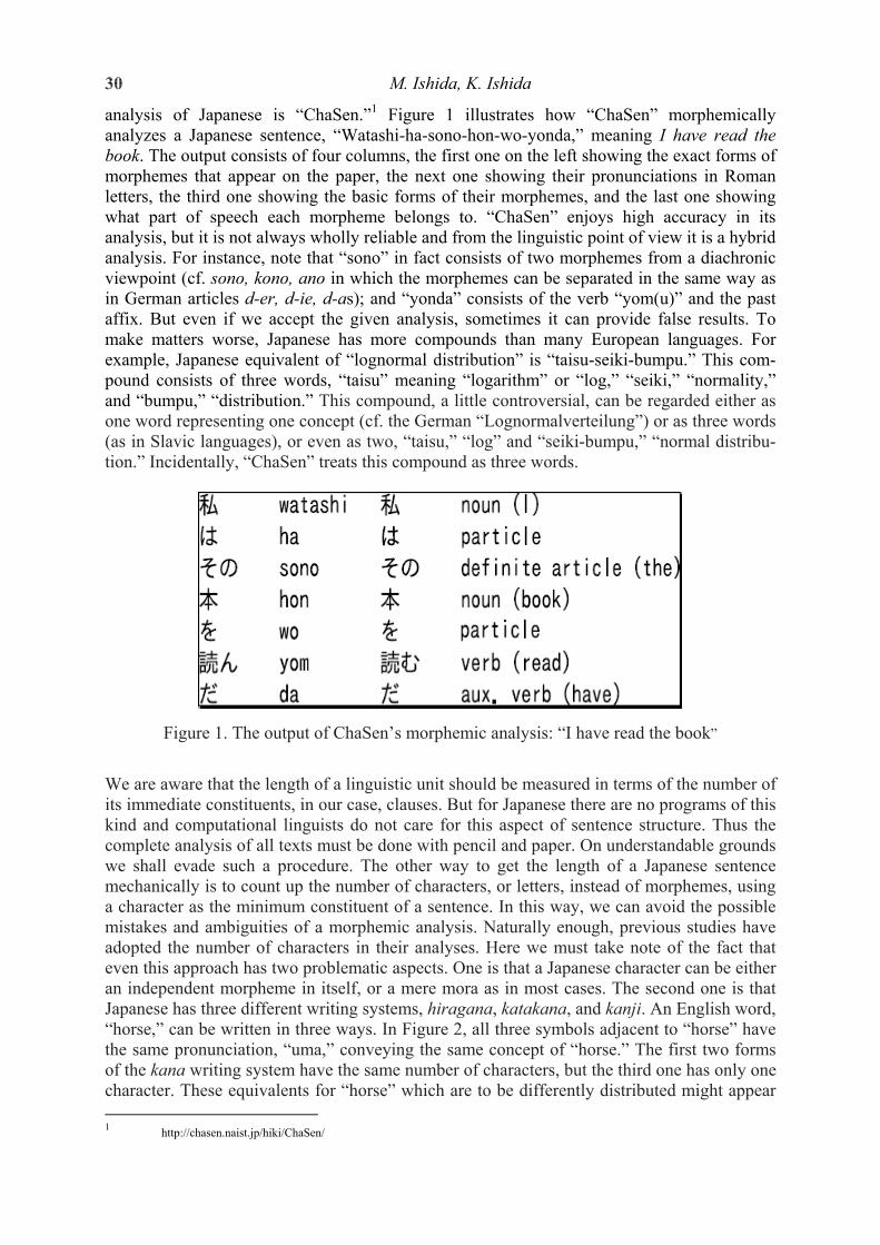
M. Ishida, K. Ishida 30
analysis of Japanese is “ChaSen.”1 Figure 1 illustrates how “ChaSen” morphemically analyzes a Japanese sentence, “Watashi-ha-sono-hon-wo-yonda,” meaning I have read the book. The output consists of four columns, the first one on the left showing the exact forms of morphemes that appear on the paper, the next one showing their pronunciations in Roman letters, the third one showing the basic forms of their morphemes, and the last one showing what part of speech each morpheme belongs to. “ChaSen” enjoys high accuracy in its analysis, but it is not always wholly reliable and from the linguistic point of view it is a hybrid analysis. For instance, note that “sono” in fact consists of two morphemes from a diachronic viewpoint (cf. sono, kono, ano in which the morphemes can be separated in the same way as in German articles d-er, d-ie, d-as); and “yonda” consists of the verb “yom(u)” and the past affix. But even if we accept the given analysis, sometimes it can provide false results. To make matters worse, Japanese has more compounds than many European languages. For example, Japanese equivalent of “lognormal distribution” is “taisu-seiki-bumpu.” This com-pound consists of three words, “taisu” meaning “logarithm” or “log,” “seiki,” “normality,” and “bumpu,” “distribution.” This compound, a little controversial, can be regarded either as one word representing one concept (cf. the German “Lognormalverteilung”) or as three words (as in Slavic languages), or even as two, “taisu,” “log” and “seiki-bumpu,” “normal distribu-tion.” Incidentally, “ChaSen” treats this compound as three words.
Figure 1. The output of ChaSen’s morphemic analysis: “I have read the book” We are aware that the length of a linguistic unit should be measured in terms of the number of its immediate constituents, in our case, clauses. But for Japanese there are no programs of this kind and computational linguists do not care for this aspect of sentence structure. Thus the complete analysis of all texts must be done with pencil and paper. On understandable grounds we shall evade such a procedure. The other way to get the length of a Japanese sentence mechanically is to count up the number of characters, or letters, instead of morphemes, using a character as the minimum constituent of a sentence. In this way, we can avoid the possible mistakes and ambiguities of a morphemic analysis. Naturally enough, previous studies have adopted the number of characters in their analyses. Here we must take note of the fact that even this approach has two problematic aspects. One is that a Japanese character can be either an independent morpheme in itself, or a mere mora as in most cases. The second one is that Japanese has three different writing systems, hiragana, katakana, and kanji. An English word, “horse,” can be written in three ways. In Figure 2, all three symbols adjacent to “horse” have the same pronunciation, “uma,” conveying the same concept of “horse.” The first two forms of the kana writing system have the same number of characters, but the third one has only one character. These equivalents for “horse” which are to be differently distributed might appear 1 http://chasen.naist.jp/hiki/ChaSen/

Sentence length distribution in Japanese 31
in one and the same Japanese sentence. Sentence length should be a fixed (invariant) quantity. In this sense, the fact that a choice of a writing system would possibly have a significant influence on the sentence length distribution simply casts doubts on the validity of the char-acter as a counting unit. There is one more possibility to be taken into consideration: the phoneme. But phonemes are not immediate constituents of sentence and the support of the random variable “length” would contain so many values that many of them would have the frequency zero. This automatically leads to a senseless multimodal distribution having no relevance to the analysis.
Figure 2. The three ways of writing “horse” in Japanese
In collecting data on Japanese sentence lengths, there is one further question other than the selection of a measurement unit: It is the question of whether dialogue can be analyzed in the exactly same way as narrative. Mizutani (1957) pointed out that both description and dialogue in literary works have their own distributions and parameters, for example, the former following a normal distribution, and the latter, a gamma distribution. This is, however, Mizutani’s mere speculation, not verified by any further experiments and, as said above, the first approximation of a kind.
Having taken into account all problematic elements, we have examined a considerable number of Japanese writers’ works. This time we have relied upon “ChaSen” automatically measuring all the sentence lengths of each entire text, and the number of each-sentence mor-phemes resulting from its analysis has been employed without any alteration. Using the theor-etical approaches of G.K. Zipf (1949) and his followers in later years, we conjectured that there should be a kind of self-regulation of sentence lengths connecting the neighbouring classes by a proportionality function (cf. Altmann and Köhler 1996), i.e.
(1) 1( )x xP g x P −= Here g(x) = f(x)/h(x). Now, f(x) can be interpreted as the (diversification) force of the speaker, his subconscious endeavour to make his speech production as easy as possible. However, taken to an extreme, this would destroy any communication. Thus this self-organizing force must be controlled by the hearer (or the community), by a self-regulating function h(x). Both must be constructed in such a way that the probability distribution converges. In a simple and very general case we let f(x) = a + bx and h(x) = c + dx. Inserting them in (1) we obtain
(2) 1 1( ) ( / )( ) ( / ) 1x x x
f x a bx a b x bP P Ph x c dx c d x d xP− − −
+ += = =
+ + .
Replacing a/b = k-1, c/d = m-1 and b/d = q (0 < q < 1) we obtain (k and m must fulfil some special conditions)
(3) 111x x
k xP qm x −+ −
=+ −
P . Solving this simple difference equation we obtain the Hyperpascal distribution

M. Ishida, K. Ishida 32
(4) 0
1
1x
x
k x
xP
m x
x
+ − =
+ −
q P , x = 0,1,2,…
where 10 2 1( ,1; , )P F k m− = q and F(.) is the hypergeometric function. It has been shown (cf.
Altmann 1988) that this distribution is adequate if sentence length is not measured in terms of the number of immediate constituents, whereas in terms of that of clauses, the negative bin-omial is adequate. The Hyperpascal distribution builds a family, some members of which (Poisson, geometric, Katz family, shifted logarithmic, Hyperpoisson, Waring, Yule etc.) are employed in different domains of linguistics. And it is interesting to see that its continuous counterpart is Pearson’s Type III distribution, i.e. the generalized gamma distribution (cf. Mačutek and Altmann 2007). Thus using special kinds of gamma distribution is a continuous approximation to the solution of the problem. In both cases (discrete or continuous), we must perform an a priori pooling of classes for shorter texts because many classes are represented very insufficiently. Pearson Type III would require numerical integration with optimization, while a ready made software will be available, if one decides to work with the Hyperpascal.
Consider the data “aitobi3 [Osamu Dazai’s Ai to Bi nitsuite]” presented in Table 1.
Table 1 The raw data of the file “aitobi3”
X f(X) X f(X) X f(X) X f(X) 1 2 3 4 5 6 7 8 9 10 11 12 13 14 15 16 17 18 19 20 21 22 23 24 25
1 0 8 9 3 21 10 14 6 7 8 6 5 6 6 3 5 1 3 1 0 3 1 6 0
26 27 28 29 30 31 32 33 34 35 36 37 38 39 40 41 42 43 44 45 46 47 48 49 50
1 0 4 1 1 1 4 1 1 0 0 0 0 1 0 1 1 1 0 0 0 1 0 0 0
51 52 53 54 55 56 57 58 59 60 61 62 63 64 65 66 67 68 69 70 71 72 73 74 75
0 0 1 0 0 1 0 0 0 0 0 0 0 0 0 1 0 0 0 0 0 0 0 0 0
76 77 78 79 80 81 82 83 84 85 86 87 88 89 90 91 92 93 94 95 96 97 98 99 100
0 0 0 0 0 0 0 0 0 0 0 0 0 0 0 0 0 0 0 0 0 0 0 0 1

Sentence length distribution in Japanese 33
As can be seen, the individual classes are not sufficiently occupied, thus a number of modes are present and the fitting of any discrete distribution would be rather a very raw approximation. The data is presented graphically in Figure 3. In a situation like this, one usually pools some classes in order to obtain expected values at least greater than 1. This can be done either before or after applying a theoretical distribution. We shall do it before the analysis. We first choose an interval of three values, i.e. pool the classes 1-2-3, 4-5-6, 7-8-9, …and let the class be represented by its mean, i.e. X = 2, 5, 8, 11, 14,…. Then we define a new variable, x = (X – 2)/3 whose support is x = 0,1,2,3,…. Filling the frequency values in the given intervals, we obtain a smoothed distribution presented in Table 2. The expected values of the Hyperpascal distribution are shown in the third column of Table 2 and a graphic picture of the fit is shown in Figure 4. It can be inferred that greater smoothing intervals would lead to a still better fitting.
Figure 3. Raw data of sentence lengths in the file „aitobi3 [Ai to Bi nitsuite]“
Table 2
Smoothed data and the theoretical values
x f(x) NP(x) x f(x) NP(x) x f(x) NP(x) 0 1 2 3 4 5 6 7 8 9 10 11
9 33 30 21 17 9 7 10 1 6 6 1
8.48 29.86 25.94 21.07 16.71 13.09 10.17 7.87 6.06 4.66 3.57 2.74
12 13 14 15 16 17 18 19 20 21 22 23
1 2 1 1 0 1 1 0 0 0 1 0
2.09 1.60 1.22 0.93 0.71 0.54 0.41 0.31 0.24 0.18 0.14 0.10
24 25 26 27 28 29 30 31 32 33
0 0 0 0 0 0 0 0 0 1
0.08 0.06 0.05 0.03 0.03 0.02 0.02 0.01 0.01 0.03
k = 0.2026, m = 0.0434, q = 0.7536, X² = 12.35, DF = 13, P = 0.50

M. Ishida, K. Ishida 34
Figure 4. Fitting the Hyperpascal to smoothed data
The results of fitting the Hyperpascal to all data analysed in morphemes are presented in Table 3. We preferred three kinds of intervals: 3, 5, and 7, though using other ones perhaps a still better fitting could be achieved. Actually we tried 9 and 11 besides, in a few particular cases of either direct speech or narrative as we shall see later in Table 4 and 5. But our aim was not to show exactly how a given text must be prepared in order to obtain a perfect fit. Rather we try to show that Japanese sentence lengths measured in the traditional way accord with Sherman’s law resulting in the Hyperpascal distribution (Altmann 1988). The signif-icance level has been fixed at α = 0.01.
Table 3 Fitting the Hyperpascal to sentence lengths measured morphemically: complete texts
(Intervals 3, 5, 7) (FF – fitting failed)
Writer Text Size K M Q DF X2 Prob Intervalakutagawa giwaku 276 0.1035 0.0567 0.8013 18 31.75 0.02 5 akutagawa jigokuhen 526 0.6193 0.1744 0.8656 34 50.86 0.03 3 akutagawa kaikano 298 FF akutagawa kage 333 FF akutagawa kataki 285 9.4345 2.9191 0.5083 15 18.28 0.25 3 akutagawa kuranosuke 218 7.5058 1.1591 0.3611 9 5.13 0.82 5 akutagawa oritsuto 965 2.8834 0.8834 0.4260 9 12.74 0.17 5 akutagawa rashom 160 FF akutagawa umano 374 1.8397 0.2441 0.4299 7 16.33 0.02 5 ango ishino 322 0.1787 0.0515 0.7347 13 14.75 0.32 7 arishima chiisaki 300 2.6558 0.7654 0.6784 18 20.73 0.29 3 arishima hitofusano 177 1.3649 0.3644 0.6086 10 8.18 0.61 5

Sentence length distribution in Japanese 35
arishima kajito 307 0.1623 0.0467 0.6583 10 5.11 0.88 5 arishima oyako 560 1.3034 0.2893 0.6048 13 10.16 0.68 5 arishima kankan 303 1.7041 0.4752 0.6154 13 11.81 0.54 5 dazai aitobi 454 0.5679 0.4472 0.5542 7 13.56 0.06 7 dazai joseito 988 0.2281 0.1188 0.8016 25 39.86 0.03 3 dazai kamome 460 0.0384 0.0223 0.5159 6 8.61 0.20 7 dazai kirigirisu 301 0.3302 0.0738 0.7120 14 12.03 0.60 5 dazai kotenfu 444 0.3418 0.1386 0.7251 15 27.93 0.02 3 dazai merosu 471 0.1721 0.0532 0.5046 6 3.59 0.73 5 dazai oto 159 0.8497 0.5280 0.7471 13 17.81 0.17 3 dazai sado 560 0.1395 0.0489 0.5015 6 9.99 0.13 5 dazai ubasute 608 FF dazai osan 212 FF dazai kashoku 696 FF hashimoto chizu 378 1.0635 0.03384 0.5919 10 13.48 0.20 7 hirabayashi yamabuki 437 0.9106 0.3076 0.6612 14 5.86 0.97 5 hojo gantai 192 2.2442 1.0185 0.6434 12 7.80 0.80 5 hori seikazoku 435 1.1506 0.3388 0.7521 21 34.53 0.03 3 hori tabino 225 0.2257 0.0668 0.7530 15 15.73 0.40 7 hori hanao 382 FF hori banka 312 1.6980 0.6295 0.6597 14 16.00 0.31 5 hori hono 242 0.2175 0.0609 0.8409 21 17.89 0.66 5 itakura goshiki 568 1.7728 0.3777 0.5854 13 14.76 0.32 3 itakura haruno 217 6.9692 0.6865 0.2053 4 1.55 0.82 5 itakura yamato 331 0.5303 0.1434 0.6014 9 12.33 0.20 5 ito hamagiku 342 2.1256 0.3238 0.4731 9 4.02 0.91 5 ito koroku 281 2.0073 0.3486 0.6579 16 13.87 0.61 3 ito kyonen 466 FF ito nanako 283 1.3859 0.1809 0.5288 9 3.91 0.92 5 ito nogiku 975 0.5316 0.1260 0.5578 10 8.10 0.62 7 kajii deinei 242 2.3732 0.4015 0.4458 7 8.77 0.27 5 kajii fuyuhae 330 2.3847 0.5663 0.6403 16 12.28 0.72 5 kajii koubi 193 11.9507 1.4538 0.2232 6 13.27 0.04 5 kajii remon 142 0.6119 0.0727 0.7874 17 19.75 0.29 3 kajii setsugo 277 0.2736 0.1301 0.7295 14 17.01 0.26 3 katai ippei 511 1.9371 0.4552 0.3933 6 4.96 0.55 5 katai shojo 266 0.4783 0.2250 0.7607 16 9.71 0.88 5 katai tokoyo 635 0.8703 0.2359 0.7332 20 18.55 0.55 3 kikuchi emu 268 2.6557 1.0129 0.4489 6 2.97 0.81 7 kikuchi seni 297 5.1167 0.3295 0.2304 5 6.65 0.25 7 kikuchi shimabara 404 0.0394 0.0204 0.7450 15 18.34 0.25 5 kikuchi shusse 228 0.9690 0.1952 0.5241 7 6.24 0.51 7 kikuchi wakasugi 221 17.7068 1.0198 0.1526 6 5.30 0.51 7 koda shonen 114 0.1233 0.0110 0.8329 17 20.18 0.27 5 kuroshima ana 435 2.0282 0.5573 0.6166 14 14.24 0.43 3 kuroshima dempo 216 0.5852 0.2358 0.6399 10 9.13 0.52 5 kuroshima mogura 654 4.3585 0.7056 0.3205 7 13.70 0.06 5 kuroshima mon 166 0.9769 0.1241 0.3403 3 3.79 0.28 7

M. Ishida, K. Ishida 36
kuroshima nusumu 364 2.7890 0.3142 0.2367 3 1.11 0.77 7 kuroshima sato 167 0.3650 0.1321 0.5824 7 1.68 0.98 5 kuroshima tongun 252 1.6990 0.2883 0.4819 8 9.23 0.32 5 kuroshima zensho 316 1.9027 0.5389 0.3649 5 1.99 0.85 7 makino tsurube 361 FF makino kinada 279 1.7881 0.7121 0.6357 12 10.28 0.59 7 minakami yamanote 387 0.5858 0.3683 0.7696 18 13.90 0.74 5 mishima hashi 359 0.8802 0.3009 0.5449 8 8.83 0.36 7 miyamoto akarui 297 1.6922 1.3023 0.7606 17 28.31 0.04 3 miyazawa karasu 165 0.2216 0.1312 0.7984 16 18.01 0.32 3 murai sobano 179 1.6458 0.1299 0.7071 18 33.89 0.01 5 oda osaka 164 0.2717 0.0734 0.7978 16 29.21 0.02 5 oda keiba 231 0.1659 0.0387 0.7543 15 24.77 0.05 7 ogai futarino 412 34.5950 1.1263 0.0548 4 8.57 0.07 7 ogai asobi 373 2.9731 0.4692 0.2801 4 1.77 0.78 7 ogai shokudo 193 53.72 4.3131 0.0817 5 5.05 0.41 7 ogai niwatori 762 6.6721 1.1193 0.1941 4 4.07 0.40 7 ogai kazui 271 0.4945 0.1427 0.5723 8 6.69 0.57 7 okamoto karei 286 1.1520 0.3446 0.7406 18 12.74 0.81 3 okamoto kingyo 830 1.5109 0.6276 0.5896 12 20.43 0.06 7 okamoto rigyo 171 0.6448 0.2775 0.7991 19 19.11 0.45 3 okamoto sushi 366 0.8861 0.2568 0.6546 13 14.82 0.32 5 okamoto tokaido 378 0.0820 0.0438 0.6949 12 11.01 0.53 7 sasa kikansha 217 20.0666 0.5214 0.0542 2 0.73 0.70 7 sasa midori 127 1.3497 0.3012 0.6031 10 12.79 0.24 5 shimazaki shishu 316 0.8158 0.1699 0.7545 20 21.55 0.37 3 shimazaki namiki 373 0.2725 0.0881 0.6094 9 6.85 0.65 5 shimazaki fune 354 2.9653 0.5659 0.4660 9 12.08 0.21 5 shimazaki mebae 881 2.1641 0.4502 0.4824 9 3.56 0.94 5 shimazaki bumpai 497 0.8753 0.3177 0.5588 9 7.76 0.56 7 shiraki saite 236 0.6287 0.1199 0.7862 20 23.21 0.28 3 soseki buncho 411 0.8648 0.0818 0.4942 8 4.31 0.83 5 soseki hennaoto 110 0.0692 0.0158 0.7292 10 6.76 0.75 5 soseki sakubutsu 183 0.0463 0.0070 0.7325 12 6.37 0.90 5 soseki kotonone 776 1.2049 0.3660 0.4216 7 1.96 0.96 7 soseki tegami 263 0.6802 0.2308 0.6347 10 10.31 0.41 7 suzu ogon 439 20.3908 1.7829 0.1431 6 11.73 0.07 5 takiji haha 294 0.2951 0.1829 0.7342 14 10.90 0.69 5 takiji yukino 739 19.5497 8.2619 0.3997 12 9.88 0.63 3 unno daino 489 0.9564 0.2851 0.5884 10 10.41 0.41 5 unno kagaku 114 0.6669 0.1175 0.5556 6 1.81 0.94 7 unno kibutsu 466 1.2499 0.4762 0.4860 7 7.58 0.37 7 unno neon 408 1.1334 0.4731 0.5099 7 9.91 0.19 7 unno tsuki 505 0.0921 0.0394 0.8025 22 28.00 0.18 3 watanabe uso 300 0.2824 0.1313 0.6904 12 7.11 0.85 5 watanabe akai 197 2.0690 0.5612 0.5421 9 7.80 0.55 5 watanabe aruhaha 193 2.8232 1.0305 0.4449 6 9.30 0.16 7 watanabe shohai 298 0.5499 0.1965 0.6890 12 9.22 0.68 5

Sentence length distribution in Japanese 37
yamada musashino 351 0.3253 0.1736 0.8413 26 21.01 0.74 3 yamashita ruten 116 1.2913 0.0707 0.6484 12 16.08 0.19 5 yokomitsu kikaiy 244 FF yokomitsu jikan 150 3.6477 0.6335 0.6743 18 19.59 0.36 7 yumeno koko 439 1.3923 0.4764 0.6191 12 14.53 0.27 5
As can be seen, out of 113 texts 103 could be captured by the Hyperpascal. Even the residual 10 data could be captured if we attempted a different priori pooling, but this is no more than a question of principle. Sometimes we even left smaller intervals if the fitting was significant. We did not try to achieve “the best fit.” We rather scrutinize the problem of distinguishing between dialogue and narrative parts. Table 4 contains the same texts, showing the result of direct speech, and followed by Table 5 showing that of narrative. However, there is a problem associated with direct speech. If it is dialogue, i.e. if there are at least two speaking persons, the author must differentiate them in some way, for example, in their sentence length. Hence dialogue has two independent parts which must not be mixed. If there are more speaking per-sons, then each speaker’s words must be evaluated separately. This kind of research might be of great interest and use for the purposes of analyzing a single work from a literary point of view. For our particular purposes, namely for corroborating a variant of Sherman’s law, it would play a merely subordinate role. The results of dialogue and narrative parts are given below consecutively. In respect of direct speech, there are a dozen texts that contain no dial-ogue data (ND) and as many texts that do not have enough data to fit the Hyperpascal (NED), and there are four texts where the fitting failed (FF).
Table 4 Direct speech (Intervals 3, 5, 7, 9, 11)
Writer Text Size K M Q DF X2 P Interv. akutagawa giwaku 44 FF akutagawa jigokuhen 114 0.1816 0.1033 0.4837 4 1.27 0.87 7 akutagawa kage 116 0.1826 0.1846 0.5044 3 2.25 0.52 7 akutagawa kaikano 188 20.2672 3.6874 0.2500 9 15.87 0.07 9 akutagawa kataki 36 6.2749 0.4248 0.1614 2 0.40 0.82 5 akutagawa kuranosuke 79 22.9651 1.448374 0.1061 3 0.47 0.93 7 akutagawa oritsuto 462 0.2653 0.121514 0.3137 2 2.09 0.35 7 akutagawa rashom 26 1.3298 0.393276 0.5471 4 5.08 0.28 5 akutagawa umano 132 0.1818 0.049125 0.4942 4 10.92 0.03 5 ango ishino NED arishima chiisaki NED arishima hitofusano 35 FF arishima kajito 53 2.2645 1.3530 0.3170 1 0.30 0.59 7 arishima kankan 37 1.5100 1.2894 0.6497 5 5.14 0.40 5 arishima oyako 199 0.4421 0.2238 0.5669 6 2.07 0.91 7 dazai aitobi 298 0.4143 0.3265 0.6619 10 12.99 0.22 5 dazai joseito 58 2.5983 1.8394 0.5290 4 3.86 0.43 3 dazai kamome 122 1.1527 1.2311 0.5092 3 4.83 0.18 7 dazai kashoku 209 0.1433 0.0780 0.4593 4 9.23 0.06 5 dazai kirigirisu NED dazai kotenfu 187 0.2690 0.1160 0.7351 13 18.14 0.15 3 dazai merosu 168 0.4932 0.1373 0.3484 3 0.77 0.86 5

M. Ishida, K. Ishida 38
dazai osan 96 1.7210 3.2101 0.5548 1 2.95 0.086 9 dazai oto 38 0.7478 0.7053 0.6608 4 5.18 0.27 3 dazai sado 102 1.1612 1.2352 0.4033 1 0.76 0.38 7 dazai ubasute 208 0.0723 0.0428 0.6776 10 14.39 0.16 3 hashimoto chizu 117 4.1328 1.9360 0.5181 7 4.30 0.75 5 hirabayashi yamabuki 184 1.1526 0.5655 0.5887 8 1.03 0.998 5 hojo gantai 39 0.6168 0.4457 0.5251 3 1.52 0.68 5 hori banka 54 3.1609 0.9597 0.2349 1 0.13 0.72 7 hori hanao 31 0.3769 0.1168 0.6588 6 5.96 0.43 3 hori hono 152 1.5339 0.7042 0.7066 13 9.58 0.73 7 hori seikazoku 57 1.7604 0.4201 0.4760 5 2.21 0.82 3 hori tabino NED itakura goshiki NED itakura haruno NED itakura yamato NED ito hamagiku 84 1.5591 0.3012 0.4500 5 3.24 0.66 5 ito koroku 111 0.0454 0.0180 0.4796 3 1.60 0.66 7 ito kyonen 35 0.7758 0.1511 0.4300 2 0.75 0.69 5 ito nanako 29 15.9699 1.2484 0.1563 3 1.16 0.76 3 ito nogiku 393 0.1374 0.0317 0.6467 10 18.21 0.05 5 kajii deinei ND kajii fuyuhae ND kajii koubi ND kajii remon ND kajii setsugo ND katai ippei 95 0.5172 0.1831 0.4502 3 5.89 0.12 3 katai shojo 57 0.1548 0.0763 0.6293 5 1.62 0.90 5 katai tokoyo 192 0.3829 0.1211 0.6609 10 10.72 0.38 3 kikuchi emu 83 0.3832 0.1026 0.4789 3 2.715 0.44 5 kikuchi seni 85 1.715 0.2063 0.1747 1 1.29 0.26 11 kikuchi shimabara 214 0.3771 0.1867 0.5792 7 12.26 0.09 5 kikuchi shusse 34 0.0994 0.0165 0.4302 2 0.34 0.84 5 kikuchi wakasugi 11 FF koda shonen ND kuroshima ana 108 0.4544 0.1806 0.3687 1 4.18 0.04 5 kuroshima dempo 80 0.6002 0.5297 0.6574 6 5.59 0.47 5 kuroshima mogura 153 38.946 9.1844 0.2144 7 2.38 0.94 3 kuroshima mon 62 0.1098 0.0206 0.5401 3 5.23 0.16 5 kuroshima nusumu 96 0.1706 0.1061 0.6348 6 12.08 0.06 3 kuroshima sato 68 0.2488 0.0922 0.6740 6 14.66 0.02 3 kuroshima tongun 61 1.4061 0.2862 0.2784 1 0.96 0.33 5 kuroshima zensho 74 2.3327 2.6170 0.7587 8 3.02 0.93 3 makino kinada 89 0.5892 0.1421 0.7448 12 14.78 0.25 3 makino tsurube 157 1.5685 1.3012 0.5458 5 7.30 0.20 7 minakami yamanote 102 0.1527 0.0598 0.2744 1 0.40 0.53 7 mishima hashi 74 0.3204 0.1001 0.3467 1 4.76 0.03 5 miyamoto akarui 113 1.7018 1.5909 0.6519 6 2.97 0.81 3 miyazawa karasu 62 0.4617 0.2967 0.5867 4 2.86 0.58 3

Sentence length distribution in Japanese 39
murai sobano ND oda keiba NED oda osaka NED ogai asobi 65 4.1224 5.8304 0.7282 3 6.05 0.11 5 ogai futarino 56 1.7175 1.4188 0.6062 4 4.63 0.33 5 ogai kazui 65 0.2298 0.1528 0.5261 3 3.02 0.39 5 ogai niwatori 175 0.9699 1.0521 0.4804 3 8.79 0.03 7 ogai shokudo 102 1.6770 0.5108 0.4607 5 3.40 0.64 7 okamoto karei 92 0.0462 0.0101 0.7534 10 8.29 0.60 3 okamoto kingyo 198 0.0338 0.0243 0.7854 13 22.56 0.05 3 okamoto rigyo 52 2.0128 1.6204 0.5564 2 3.00 0.22 5 okamoto sushi 78 0.3798 0.1484 0.4783 3 5.49 0.14 5 okamoto tokaido 102 0.0672 0.0225 0.8015 14 7.20 0.93 3 sasa kikansha 102 FF sasa midori 53 3.3945 0.7119 0.3239 3 0.74 0.86 7 shimazaki bumpai 120 1.6281 0.2471 0.2613 2 1.54 0.46 5 shimazaki fune 34 0.3927 0.1668 0.5610 3 2.87 0.41 5 shimazaki mebae 142 1.4990 0.8369 0.6176 8 11.57 0.17 3 shimazaki namiki 156 0.4712 0.1523 0.4678 5 4.20 0.52 5 shimazaki shishu 33 2.9693 0.5955 0.3710 3 1.93 0.59 5 shiraki saite 38 0.3329 0.0478 0.5619 4 4.63 0.33 3 soseki buncho NED 7 soseki hennaoto 28 0.3773 0.2522 0.5495 2 0.56 0.76 5 soseki kotonone 375 0.0813 0.0264 0.6194 9 3.38 0.95 5 soseki sakubutsu ND 7 soseki tegami 52 35.634 2.1977 0.0910 4 3.59 0.46 3 suzu ogon 115 2.4353 0.1166 0.2720 3 1.84 0.61 5 takiji haha 83 0.6368 0.3612 0.6280 6 10.18 0.12 5 takiji yukino 174 0.6376 0.5780 0.4857 4 4.2 0.38 3 unno daino 200 0.8300 0.3943 0.5754 7 2.3 0.94 5 unno kagaku NED 7 unno kibutsu 216 1.3625 1.0254 0.7349 14 9.89 0.77 3 unno neon 226 0.2116 0.1524 0.6677 9 4.54 0.87 5 unno tsuki 245 0.1203 0.0556 0.6774 10 6.17 0.80 3 watanabe akai NED watanabe aruhaha ND watanabe shohai ND watanabe uso 164 0.6077 0.5130 0.5353 5 3.28 0.66 7 yamada musashino 185 0.4815 0.5999 0.6410 6 5.24 0.51 7 yamashita ruten 90 3.2763 0.3158 0.3972 6 7.10 0.31 7 yokomitsu jikan ND yokomitsu kikaiy ND yumeno koko 137 0.3294 0.2449 0.8120 16 16.59 0.41 3

M. Ishida, K. Ishida 40
Table 5 Narrative (Intervals 3, 5, 7, 9, 11)
Writer Text Size K M Q DF X2 P akutagawa giwaku 232 3.2508 0.7474 0.4755 9 11.81 0.22 7 akutagawa jigokuhen 412 1.7096 0.3189 0.6290 13 26.62 0.01 7 akutagawa kage 217 12.0019 0.8216 0.2260 7 11.47 0.12 5 akutagawa kaikano 110 1.4427 0.2013 0.5610 7 9.97 0.19 7 akutagawa kataki 249 527.7755 1.9709 0.0087 7 13.24 0.07 5 akutagawa kuranosuke 139 5.9010 0.3954 0.3701 9 2.28 0.99 5 akutagawa oritsuto 503 FF akutagawa rashom 134 FF akutagawa umano 242 11.2705 0.2983 0.15839 5 7.36 0.20 5 ango ishino 318 0.1412 0.0388 0.7412 13 14.82 0.32 7 arishima chiisaki 297 3.9009 1.1110 0.6215 17 18.79 0.34 3 arishima hitofusano 142 2.0363 0.2829 0.5584 10 4.81 0.90 5 arishima kajito 254 0.5221 0.1362 0.5169 6 3.56 0.74 7 arishima kankan 266 0.3565 0.0729 0.6264 9 6.06 0.73 7 arishima oyako 361 4.0829 0.9981 0.6000 17 9.78 0.91 3 dazai aitobi 156 0.5603 0.3690 0.5256 5 4.85 0.43 7 dazai joseito 930 0.2664 0.1216 0.8011 25 38.53 0.04 3 dazai kamome 338 0.1819 0.0760 0.4907 5 7.05 0.22 7 dazai kashoku 487 0.0963 0.0275 0.6607 11 17.94 0.08 5 dazai kirigirisu 299 0.3799 0.0815 0.7082 14 12.30 0.58 5 dazai kotenfu 257 0.4089 0.1571 0.6982 12 14.66 0.26 3 dazai merosu 303 0.3224 0.0806 0.5184 6 4.00 0.68 5 dazai osan 116 0.3899 0.1703 0.8125 17 33.73 0.01 7 dazai oto 121 0.2934 0.1345 0.5840 6 8.65 0.19 7 dazai sado 458 0.2872 0.0790 0.4953 6 11.47 0.07 5 dazai ubasute 400 0.4038 0.2527 0.4846 5 14.88 0.01 7 hashimoto chizu 261 0.6289 0.1289 0.6293 10 11.99 0.29 7 hirabayashi yamabuki 253 0.8716 0.0803 0.6629 13 5.46 0.96 5 hojo gantai 153 2.0267 0.2963 0.5915 11 7.67 0.74 5 hori banka 258 6.6566 2.5129 0.6290 19 14.07 0.78 3 hori hanao 351 1.1630 0.1029 0.8032 29 35.43 0.19 3 hori hono 90 0.1972 0.0369 0.8306 17 14.45 0.63 5 hori seikazoku 378 1.7554 0.3774 0.7199 20 35.53 0.02 3 hori tabino 217 0.2795 0.0572 0.7479 15 16.16 0.37 7 itakura goshiki 532 0.5177 0.0946 0.3713 4 3.66 0.45 7 itakura haruno 214 9.7424 0.7743 0.1661 4 1.47 0.83 5 itakura yamato 309 0.6158 0.1083 0.5859 9 11.63 0.23 5 ito hamagiku 258 2.5754 0.3032 0.4484 8 2.97 0.94 5 ito koroku 170 1.5610 0.0512 0.4003 6 3.13 0.79 7 ito kyonen 431 1.6990 0.1969 0.3002 4 9.27 0.05 9 ito nanako 254 2.8372 0.2986 0.4302 8 7.76 0.46 5 ito nogiku 582 1.8452 0.2851 0.4589 8 9.78 0.28 7 kajii deinei 222 5.1011 0.4674 0.3167 7 10.22 0.18 5 kajii fuyuhae 305 2.3021 0.3570 0.6201 15 9.47 0.85 3

Sentence length distribution in Japanese 41
kajii koubi 187 3.7351 0.5448 0.3925 7 14.88 0.04 5 kajii remon 134 1.360 0.1093 0.7077 15 18.87 0.22 3 kajii setsugo 180 0.6015 0.1389 0.7129 13 16.01 0.25 3 katai ippei 416 0.5105 0.0858 0.3799 4 3.87 0.42 7 katai shojo 209 0.5526 0.1179 0.8481 27 22.16 0.73 3 katai tokoyo 443 1.9931 0.2240 0.6600 18 13.79 0.74 3 kikuchi emu 185 0.2209 0.0580 0.7372 9 13.21 0.15 5 kikuchi seni 212 2.3085 0.1345 0.3451 5 4.99 0.42 7 kikuchi shimabara 190 FF kikuchi shusse 194 1.5669 0.1836 0.4743 7 6.802 0.45 7 kikuchi wakasugi 210 FF koda shonen 114 0.1233 0.0110 0.8329 17 20.18 0.27 5 kuroshima ana 327 1.9025 0.2617 0.4512 8 4.22 0.84 5 kuroshima dempo 136 1.8996 0.3230 0.6698 15 12.16 0.67 3 kuroshima mogura 501 3.5743 0.2388 0.3218 7 12.05 0.10 5 kuroshima mon 104 1.5992 0.1087 0.3088 3 3.06 0.38 7 kuroshima nusumu 268 4.0326 0.2841 0.4515 11 8.64 0.66 3 kuroshima sato 99 0.0074 0.0010 0.5192 4 1.76 0.78 7 kuroshima tongun 191 2.4103 0.1772 0.4365 8 8.02 0.43 5 kuroshima zensho 242 1.9764 0.1880 0.4369 7 3.49 0.84 5 makino kinada 190 1.3305 0.5076 0.7135 12 21.60 0.04 7 makino tsurube 204 0.5034 0.2017 0.5960 8 13.21 0.11 9 minakami yamanote 285 3.1271 0.6449 0.4968 10 15.85 0.10 7 mishima hashi 285 0.9655 0.1537 0.6460 12 10.05 0.61 5 miyamoto akarui 184 11.9772 1.3814 0.1700 4 8.57 0.07 7 miyazawa karasu 103 0.0022 0.0014 0.8347 17 28.06 0.04 3 murai sobano 179 1.6458 0.1299 0.7071 18 33.89 0.01 5 oda keiba 228 0.1002 0.0215 0.7602 15 25.33 0.05 7 oda osaka 162 0.2893 0.0806 0.7980 16 28.82 0.03 5 ogai asobi 308 3.2854 0.3025 0.2594 4 1.79 0.77 7 ogai futarino 356 6.6858 1.4855 0.4836 14 12.42 0.57 3 ogai kazui 206 1.3157 0.1693 0.4771 7 6.69 0.46 7 ogai niwatori 587 13.1228 0.7404 0.1021 4 4.21 0.38 7 ogai shokudo 91 0.2776 0.0832 0.7804 13 9.53 0.73 3 okamoto karei 194 3.5711 0.6043 0.4678 9 12.45 0.19 5 okamoto kingyo 632 3.4650 0.9013 0.5850 16 24.03 0.09 5 okamoto rigyo 119 0.2577 0.0490 0.8499 22 21.25 0.51 3 okamoto sushi 288 0.7983 0.1455 0.5572 8 8.21 0.41 7 okamoto tokaido 276 0.1071 0.0433 0.7016 12 14.70 0.26 7 sasa kikansha 115 20.8736 0.1578 0.0819 4 1.85 0.76 5 sasa midori 74 1.4028 0.1152 0.4674 5 4.05 0.54 7 shimazaki bumpai 377 1.7282 0.5855 0.6445 14 23.06 0.06 5 shimazaki fune 320 3.1831 0.4953 0.6151 17 19.83 0.28 3 shimazaki mebae 739 1.4973 0.1784 0.3944 6 1.75 0.94 7 shimazaki namiki 217 0.2989 0.0960 0.5413 6 3.64 0.73 7 shimazaki shishu 283 1.1646 0.2866 0.4810 7 6.08 0.53 7 shiraki saite 198 2.2885 0.2657 0.4015 6 3.51 0.74 7 soseki buncho 409 0.8612 0.0815 0.4941 8 4.32 0.83 5

M. Ishida, K. Ishida 42
soseki hennaoto 82 0.3567 0.2955 0.7203 8 7.60 0.47 5 soseki kotonone 401 3.2625 0.6202 0.5749 15 17.52 0.29 3 soseki sakubutsu 183 0.0463 0.0070 0.7325 12 6.37 0.90 5 soseki tegami 211 2.2489 0.3751 0.5131 9 13.03 0.16 7 suzu ogon 324 10.4524 0.5815 0.0638 2 0.89 0.64 11takiji haha 211 0.7726 0.3625 0.6113 8 16.23 0.04 7 takiji yukino 565 0.2493 0.0695 0.4080 5 6.25 0.28 7 unno daino 289 1.1157 0.1607 0.5731 10 11.29 0.34 5 unno kagaku 108 1.0242 0.1328 0.5156 6 2.15 0.91 7 unno kibutsu 250 1.7748 0.2114 0.4305 7 13.68 0.06 7 unno neon 182 1.1837 0.1312 0.4246 5 7.58 0.18 7 unno tsuki 260 1.7667 0.2264 0.4269 7 15.37 0.03 7 watanabe akai 194 2.1726 0.5709 0.5182 8 5.25 0.73 5 watanabe aruhaha 120 0.8454 0.0944 0.5616 7 8.00 0.33 7 watanabe shohai 298 0.5499 0.1965 0.6890 12 9.22 0.68 5 watanabe uso 136 0.7294 0.0809 0.5565 7 2.46 0.93 7 yamada musashino 166 0.3080 0.0362 0.7765 15 9.88 0.83 5 yamashita ruten 26 1.0755 0.2078 0.5730 5 8.74 0.12 9 yokomitsu jikan 150 3.6477 0.6335 0.6743 18 19.55 0.36 7 yokomitsu kikaiy 244 FF yumeno koko 302 2.6289 0.2347 0.4816 10 7.12 0.71 5 Results Though there are several texts (complete, dialogue, narrative) which do not accord with the Hyperpascal distribution in any case of our different pooling intervals, the overall result satisfactorily indicates that the law of sentence length distributions can also be effectively applied to Japanese. Each individual text which does not conform to the law must be studied separately. If there had been some kind of regulations or restrictive conditions in their creation, and if only these could be detected and allowed for in the analysis, it would be unlikely that such deviations should occur. In the considerable cases of direct speech, testing itself was impracticable simply because there was too little or no dialogue data. The first step in a new direction has been taken, and further development could be expected should sentence lengths be measured by counting the number of clauses. This project will follow shortly. Writers and Works Ryunosuke Akutagawa: Giwaku, Jigokuhen, Kage, Kaika no Otto, Aru Katakiuchi no
Hanashi, Aruhi no Oishi Kuranosuke, Oritsu to Kora, Rashomon, Uma no Ashi Sakaguchi Ango: Ishi no Omohi Takeo Arishima: Chiisaki mono he, Hitofusa no Budo, Kaji to Pochi, Kankan Mushi, Oyako Osamu Dazai: Ai to Bi nitsuite, Joseito, Kamome, Kashoku, Kirigirisu, Koten Fu, Hashire
Merosu, Osan, Oto nitsuite, Sado, Ubasute Goro Hashimoto: Chizu ni nai Machi Hatsunosuke Hirabayashi: Yamabuki Cho no Satsujin Tamio Hojo: Gantai Ki Tatsuo Hori: Banka, Hana wo moteru Onna, Hoo no saku Koro, Sei Kazoku, Tabi no E
Sentence length distribution in Japanese 43
Katsunobu Itakura: Goshiki Onsen Suki Nikki, Haru no Kamikochi he, Yama to Yuki no Nikki
Sachio Ito: Hamagiku, Kooroku, Kyonen, Nanako, Nogiku no Haka Motojiro Kajii: Deinei, Fuyu no Hae, Kobi, Remon, Setsugo, Katai Tayama: Ippeisotsu, Shojo Byo, Tokoyo Goyomi Kan Kikuchi: M Koshaku to Shashinshi, Seni no Tachiba, Shimabara Shinju, Shusse,
Wakasugi Saiban Cho Rohan Koda: Shonen Jidai Denji Kuroshima: Ana, Dempo, Mogura to Rakuban, Mon, Nusumu Onna, Sato Dorobo,
Tongun, Zensho Shinichi Makino: Kinada Mura, Tsurube to Gekko to Takitaro Minakami: Yamanote no Ko Yukio Mishima: Hashi Zukushi Yuriko Miyamoto: Akarui Kaihin Kenji Miyazawa: Karasu no Hokutoshichisei Masayoshi Murai: Soba no Aji to Kuikata Mondai Sakunosuke Oda: Keiba, Osaka Hakken Ogai Mori: Asobi, Futari no Tomo, Kazuisuchika, Niwatori, Shokudo Kanoko Okamoto: Karei, Kingyo Ryoran, Rigyo, Sushi, Tokaido Gojusantsugi Toshiro Sasaki: Kikansha, Midori no Me Toson Shimazaki: Bumpai, Fune, Mebae, Namiki, Shishu Shizu Shiraki: Saite yuku Hana Soseki Natsume: Buncho, Henna Oto, Koto no Sorane, Sakubutsu no Hihyo, Tegami Miekichi Suzuki: Ogon Cho Takiji Kobayashi: Hahatachi, Yuki no Yoru Juza Unno: Daino Shujutsu, Kagaku ga Heso wo mageta Hanashi, Kibutsudo Jiken, Neon
Yokocho Satsujin Jiken, Tsuki no Sekai Tankenki On Watanabe: Akai Entotsu, Aru Haha no Hanashi, Shohai, Uso Bimyo Yamada: Musashino Risaburo Yamashita: Ruten Riichi Yokomitsu: Jikan, Kikai Kyusaku Yumeno: Kokonatto no Mi (All the texts above were downloaded from http://www.aozora.gr.jp/index.html, with the ex-ception of Yukio Mishima's “Hashi Zukushi.” This one, still in copyright, was from Shincho-Bunko no 100 Satsu: CD-ROM Version, 1995.) References
Altmann, Gabriel (1988). Verteilungen der Satzlängen. Glottometrika 9, 147–169. Altmann, Gabriel; Köhler, Reinhard (1996). „Language Forces“ and synergetic modelling
of language phenomena. Glottometrika 15, 62-76. Arai, Hiroshi (2001). On lognormal distributions of sentence length. Hitotsubashi University
Journal 125(3), 75–100. (In Japanese). Cohen, Jacob (1988). Statistical Power Analysis for the Behavioral Sciences. New York:
Lawrence Erlbaum Associates, 2nd edition. Fucks, Walther (1968). Nach allen Regeln der Kunst. Stuttgart: Deutsche Verlagsanstalt. Grotjahn, Rüdiger; Altmann, Gabriel (1993). Modelling the distribution of word length:
some methodological problems. In: Reinhard Köhler; Burghard B. Rieger (eds.),

M. Ishida, K. Ishida 44
Contributions to Quantitative Linguistics: 141-153. Dordrecht/Boston/London: Kluwer Academic Publishers.
Kelih, Emmerich; Peter Grzybek (2004). Häufigkeit von Satzlängen: Zum Faktor der Intervallgröße als Einflussvariable. Glottometrics 8, 23–41.
Kelih, Emmerich; Peter Grzybek (2005). Satzlänge: Definition, Häufigkeiten, Modelle. Zeitschrift für Computerlinguistik und Sprachtechnologie 20(2), 31–51.
Kjetsaa, Geir (1978). The Battle of The Quiet Don: Another Pilot Study. Computers and the Humanties 11, 341–346.
Mačutek, Jan; Altmann, Gabriel (2007). Discrete and continuous modelling in quantitative linguistics. Journal of Quantitative Linguistics 14(1), 81-91.
Mizutani, Shizuo (1957). Notes to distributions of sentence length. Mathematical Linguistics, 2, 22–23. (In Japanese).
Niehaus, Brigitta (1997). Untersuchung zur Satzlängenhäufigkeit im deutschen. Glotto-metrika 16, 213-275.
Sasaki, Kazue (1976). On distributions of sentence length. Mathematical Linguistics 78, 13–22. (In Japanese).
Sichel, H.S. (1974). On a distribution representing sentence-length in written prose. Journal of the Royal Statistical Society. Vol. 1, No. 137, 25–34.
Sichel, H.S. (1975). On a distribution law for word frequencies. Journal of the American Statistical Association, Vol. 70, No. 351, 542–547.
Sigurd, Bengt; Mats Eeg-Olosson (2004). Word length, sentence length and frequency – Zipf revisited. Studia Linguistica, Vol. 1, No. 58, 37–52.
Strehlow, Michael (1997). Satzlängen in pädagogischen Fachartikeln des 19. Jahrhunderts. Staatsexamensarbeit, Göttingen.
Williams, C. B. (1940). A note on the statistical analysis of sentence-length as a criterion of literary style. Biometrika 31, 356–361.
Wittek, Martin (2001). Zur Entwicklung der Satzklänge im gegenwärtigen Deutschen. In: Best, K.-H.. (ed.), Häufigkeitsverteilungen in texten: 219-247. Trier: WVT.
Yasumoto, Biten (1965). Introduction to Sentence Psychology, Tokyo: Seishin-Publisher.( In Japanese).
Yasumoto, Biten (1966). Frontier of Sentence Psychology. Tokyo: Seishin-Publisher. (In Japanese).
Yule, George Udny (1939). On sentence-length as a statistical characteristic of style in prose: with application to two cases of disputed authorship. Biometrika 30, 363–390.
Zipf, George K. (1949). Human behavior and the principle of least effort. Cambridge: Addison-Wesley.

Glottometrics 15, 2007, 45-52
Confidence intervals and tests for the h-point and related text characteristics
Ján Mačutek1 2, Bratislava
Ioan-Iovitz Popescu, Bucharest Gabriel Altmann, Lüdenscheid
Abstract. Confidence intervals and tests for recently introduced text characteristics (the h-point and its relatives) are derived. Keywords: text analysis, h-point, a- indicator 1. Introduction The h-point was suggested by Hirsch (2005) as an index of research productivity (mainly) in physics. Popescu (2007) uses it in linguistics as a point which separates highly frequent synsemantic (or auxiliary) words from autosemantic words with lower frequencies. Popescu and Altmann (2006) introduce other three text characteristics – the k-point, the m-point and the n-point, which are modifications or analogies of the h-point applied to the frequency spec-trum, the cumulative distribution or the reverse order rank-frequency distribution. All four of them can be used to measure vocabulary richness of texts, text coverage, text compactness, analytism and synthetism of language, and so on.
Synsemantic words are usually concentrated in the first classes of the rank-frequency dis-tribution, while much more numerous autosemantic words tend to have significantly lower frequencies. However, there is no sharp boundary separating these two branches; in texts there are a few very frequent autosemantics (they build the theme of the text: see Popescu, Best and Altmann 2007), and/or some synsemantics with low frequencies which may have synonyms used alternately. Therefore we derive confidence intervals for the above mentioned character-istic points. The intervals should cover the area where synsemantics and autosemantics are mixed. 2. Confidence intervals The h-point is an extension of the mathematical fixed point to the actual discrete rank-frequency distribution, f = f(r) (of words in our case), that is by definition is the point (r, f(r)) where (if such a point does not exist in the actual distribution, one takes that r whose absolute difference to f(r) is minimum). Table 1 (see below) contains rank-frequency dis-tribution of word forms in Goethe’s poem “Erlkönig”. The table is presented in Popescu and Altmann (2006).
hhf =)(
1 Address correspondence to: [email protected] 2 Supported by research grant VEGA 1/3016/06.

J. Mačutek, I.-I. Popescu, G. Altmann 46
Table 1 Erlkönig
Rank
r Frequency
f(r) Cumulative frequency
cf(r)
Relative cumulative frequency
F(r)
Rank r
Frequency f(r)
Cumulative frequency
cf(r)
Relative cumulative frequency
F(r) 1 2 3 4 5 6 7 8 9 10 11 12 13 14 15 16 17 18 19 20
11 9 9 7 6 6 5 5 4 4 4 4 4 4 4 3 3 3 3 3
11 20 29 36 42 48 53 58 62 66 70 74 78 82 86 89 92 95 98 101
0.0489 0.0889 0.1289 0.1600 0.1867 0.2133 0.2356 0.2578 0.2756 0.2933 0.3111 0.3289 0.3467 0.3644 0.3822 0.3956 0.4089 0.4222 0.4356 0.4489
21 22 23 24 25 26 27 28 29 30 31 32 33 34 35 36 37 38 39 40-
124*
3 2 2 2 2 2 2 2 2 2 2 2 2 2 2 2 2 2 2 1
104 106 108 110 112 114 116 118 120 122 124 126 128 130 132 134 136 138 140 225
0.4622 0.4711 0.4800 0.4889 0.4978 0.5067 0.5156 0.5244 0.5333 0.5422 0.5511 0.5600 0.5689 0.5778 0.5867 0.5956 0.6044 0.6133 0.6222 1
* The ranks 40 to 124 have frequency 1 It is easy to see that the h-point is 6, as 6)6( =f . We have 225=N and . 2133.0)( =hF
Now, let h be the h-point, the cumulative probability at h and the number of val-ues which are less or equal to h. can attain the values with the probabilities which can be derived from (and explained by) an urn scheme consideration. Suppose we randomly place N balls into V urns labeled 1 . Divide the urns into two groups – the “synsemantic group” consists of the urns 1 , while the urns h
hcp hX
h,1 +
hX N,,2,1,0 K
V,,2, K
h,,K2, V,,2 K+ belong to the “autosemantic group”. We do not know (and do not need) the probabilities that a ball will be put into a particular urn. All we need is the probability that a ball will be placed into the “synsemantic group” of urns, which is the sum of probabilities of all the urns from that group (or, in other words, it is the cumulative probability at h, i.e., ). The probability of putting a ball into the “autosemantic group” of urns is, of course, uniquely determined by the previous one; it is equal to 1 .
hcp
hcp−0=hX (i.e., all balls are in the “autosemantic group” of urns) with the probability
( ) ( N
hh cpXP −== 10 ) ,
1=hX (i.e., one ball is in the “synsematic group”, all the other balls are in the “autosemantic group”) with the probability

Confidence intervals and tests for the h-point 47
( ) ( ) 11 11
Nh h
NP X cp cph
− = = −
, etc;
in general
. ( ) ( ) NrcpcprN
rXP rNh
rhh ,,2,1,0,1 K=−
== −
Hence, has the binomial distribution with the parameters N and . We note that in general the considered urn scheme is not a non-increasing distribution and the confidence interval is approximate only.
hX hcp
Denote the estimation of , i.e., is the relative cumulative frequency at h. The binomial distribution can be approximated by the normal distribution. In the next step we obtain the confidence intervals for :
ˆhcp hcp
hcp
ˆhcp
( ) ( )
1 12 2
ˆ ˆ ˆ ˆ1 1ˆ ˆ 1h h h h
h h h
cp cp cp cpP cp u cp cp u
N Nα α α− −
− − − ≤ ≤ +
= − , (1)
where α is the significance level and u is the quantile of the standard normal distribu-tion which can be found in any statistical tables or statistical software. The probability remains unchanged if we multiply in (1) all three expressions in the parentheses by N:
1 / 2α−
( ) ( )1 1
2 2
ˆ ˆ ˆ ˆ ˆ1 1h h h h h hP Ncp u Ncp cp Ncp Ncp u Ncp cpα α− −
− − ≤ ≤ + −
ˆh = 1-α (2)
We have obtained the confidence interval for cumulative frequencies at the h-point. The interval, where the cumulative frequencies from (2) are attained, is the confidence interval for the h-point. If the cumulative frequencies do not attain exactly the values equal to the confidence interval limits, we suggest taking the highest frequency below the lower interval limit, and the lowest frequency above the upper interval limit.
In the “Erlkönig” we have cp 0.2133 and N = 225. For ˆ = 05.0=α the interval (2) (i.e., the confidence interval for cumulative probabilities) yields (35.95, 60.04). We have cf(3) = 29, cf(4) = 36 and cf(8) = 58, cf(9) = 62. Hence, [3,9] is at least 95% confidence interval for the h-point.
Confidence intervals for the k-point, m-point and n-point (all of them defined in Popescu and Altmann 2006) can be constructed in the same way, using, of course, the respective cumulative probabilities and cumulative frequencies. 3. Tests
3.1. Test for cumulative probabilities corresponding to h-points The approach from the previous section can also be applied to obtain a test for comparing cumulative probabilities corresponding to h-points in two different texts.
Consider two texts. Let h denote their h-points, the cumulative probabilities 21 , h 21 , hh cpcp

J. Mačutek, I.-I. Popescu, G. Altmann 48
at (with cp being their estimations) and the numbers of word forms or lemmas in the texts, respectively. The statistic
21 , hh 1ˆ ˆ,h cp 2h 21 , NN
1
1 1
N
cpcp
cp
hh −
∧∧
∧
U
ofnumber
2
221
21
1
N
cpcp
cp
hh
hh
−
+
−=
∧∧
∧
(3)
has approximately the standard normal distribution. Hence, in terms of corresponding cumul-ative probabilities, two h-points are significantly different if 1 / 2U u α−> . Recall once more that (3) is a test for comparing cumulative probabilities corresponding to the h-points, not for comparing the h-points themselves. In other words, (3) can be used to test whether the ratios
( ))(lemmasformswordallofnumber
hthanhighersfrequenciewithlemmasformsword
in the texts under consideration are significantly different.
As an example, we test the difference of cumulative probabilities corresponding to the h-points in two poems – Goethe’s “Erlkönig” (see Table 1 above) and Moericke’s “Peregrina” (the rank-frequency distribution of word forms is presented in Table 2).
Table 2
Peregrina Rank
r Frequency
f(r) Cumulative frequency
cf(r)
Relative cumulativefrequency
F(r)
Rankr
Frequencyf(r)
Cumulative frequency
cf(r)
Relative cumulativefrequency
F(r) 1 16 16 0.0270 38 2 218 0.3676 2 16 32 0.0540 39 2 220 0.3710 3 12 44 0.0742 40 2 222 0.3744 4 12 56 0.0944 41 2 224 0.3777 5 11 67 0.1130 42 2 226 0.3811 6 10 77 0.1298 43 2 228 0.3845 7 8 85 0.1433 44 2 230 0.3879 8 8 93 0.1568 45 2 232 0.3912 9 7 100 0.1686 46 2 234 0.3946 10 7 107 0.1804 47 2 236 0.3980 11 6 113 0.1906 48 2 238 0.4013 12 6 119 0.2007 49 2 240 0.4047 13 6 125 0.2108 50 2 242 0.4081 14 6 131 0.2209 51 2 244 0.4115 15 5 136 0.2293 52 2 246 0.4148 16 5 141 0.2378 53 2 248 0.4182 17 5 146 0.2462 54 2 250 0.4216 18 5 151 0.2546 55 2 252 0.4250 19 5 156 0.2631 56 2 254 0.4283

Confidence intervals and tests for the h-point 49
20 5 161 0.2715 57 2 256 0.4317 21 4 165 0.2782 58 2 258 0.4351 22 4 169 0.2850 59 2 260 0.4384 23 4 173 0.2917 60 2 262 0.4418 24 4 177 0.2985 61 2 264 0.4452 25 4 181 0.3052 62 2 266 0.4486 26 3 184 0.3103 63 2 268 0.4519 27 3 187 0.3153 64 2 270 0.4553 28 3 190 0.3204 65 2 272 0.4287 29 3 193 0.3255 66 2 274 0.4621 30 3 196 0.3305 67 2 276 0.4654 31 3 199 0.3356 68 2 278 0.4688 32 3 202 0.3406 69 2 280 0.4722 33 3 205 0.3457 70 2 282 0.4755 34 3 208 0.3508 71 2 284 0.4789 35 3 211 0.3558 72 2 286 0.4823 36 3 214 0.3609 73 2 288 0.4857 37 2 216 0.3642 74-
378*1 593 1
* The ranks 74 to 378 have frequency 1 We have (Erlkönig) and 1 1 1ˆ6, 0.2133, 225hh cp N= = = 2 2 2ˆ8, 0.1568, 593hh cp N= = = (Per- egrina). The test (3) yields
8153.1
593)1568.01(1568.0
225)2133.01(2133.0
1568.02133.0=
−+
−−
=U
which means that for 05.0=α we do not reject the hypotheses that the cumulative prob-abilities corresponding to the h-points in these poems are equal ( 96.1975.0 =u ). 3.2. Test for a-indices The relationship between h and N can be expressed by a simple equation N = ah2 (suggested by Hirsch 2005, mentioned also in Popescu and Altmann 2006). In fact, the quantity
2
Nah
= (4)
does not depend any more on N, as can be shown using about 200 texts from 20 languages. On the contrary, index a is an indicator of language analyticity. The smaller a is, the more analytic the language is; the greater a is, the more synthetic the language is. As shown in Table 3, this statement can be corroborated empirically using 20 languages.

J. Mačutek, I.-I. Popescu, G. Altmann 50
Table 3 Mean values of a in texts of 20 languages
(from Popescu et al. 2007)
Language Mean a Language Mean a Samoan 4.56 Italian 8.41 Rarotongan 5.02 Romanian 9.15 Hawaiian 5.37 Slovenian 9.19 Maori 5.53 Indonesian 9.58 Lakota 5.69 Russian 10.10 Marquesan 5.69 Czech 10.33 Tagalog 7.24 Marathi 11.82 English 7.65 Kannada 16.58 Bulgarian 7.81 Hungarian 18.02 German 8.39 Latin 19.56
As the index a is independent of N, it can be used to compare different texts (of different lengths). We need the variances of a-indices to construct the test; hence first we look for the distributions of the h-points. As a theoretical formula is not known, and all attempts to approximate it failed, a simulation study was used.
It was shown that word rank-frequency distributions in almost all texts can be mod-eled by the right truncated zeta distribution ( , a
x cxP −= Vx ,,2,1 K= , with c being the norm-alization constant, cf. Wimmer and Altmann 1999, pp. 577-578), and its parameter can be easily estimated by Altmann-Fitter or other software.
The simulation study can be described as follows (“Erlkönig” being an example again). We generate 225 random numbers (there are 225 words in “Erlkönig”) from the right truncated zeta distribution with the parameter 0.6007 (for this parameter value the best fit is obtained) and we find the h-point for their rank-frequency distribution. The random numbers generation is repeated 100-times (i.e., we have 100 h-points from the samples with the same size and with the same distribution as word frequencies in “Erlkönig”). The a-indices for these h-points are computed and their variance is found. Finally, the process was repeated 10-times, i.e., 10 variance values (each of them being a variance of 100 a-indices) were obtained. We take their mean as the variation of the a-index.
The above mentioned numbers of generations may be considered too low, but they require quite a lot of time and our aim is to present the method only.3
Now we can test the difference between the a-indices in two texts. Denote them . The statistic
21 , aa
( ) ( )21
21
aVaraVaraa
U a+
−= (5)
has, again, approximately the standard normal distribution, i.e., the difference between a and
is significant if 1
2a 1 / 2aU u α−> .
3 A short simulation program written in R can be sent upon request ([email protected]).

Confidence intervals and tests for the h-point 51
In our texts by Goethe and Moericke we have
25.66225
221
11 ===
hNa (Erlkönig),
2656.98593
222
22 ===
hNa (Peregrina).
On the other side, by the above simulation we obtained 82.48)( 1 =aVar for “Erlkönig”
and Var for “Peregrina”, hence we finally have 05.99)( 2 =a
248.005.9982.48
2656.925.6−=
+−
=aU ,
which means that for 05.0=α the a-indices for “Erlkönig” and “Peregrina” are not signif-icantly different. 4. Examples In order to check the intralinguistic and extralinguistic differentiation of texts we performed the test for differences of cumulative probabilities corresponding to the h-points on 13 texts (by Goethe in German and Eminescu in Romanian, Table 4). The list of texts is given in the Appendix. The matrix is antisymmetric, i.e., the number in the i-th row and j-th column and the number in the j-th row and i-th column have the same absolute values but opposite signs. The critical value is ±1.96.
Table 4 U-test for the difference between cumulative probabilities
corresponding to h-points
G 05 G 09 G 10 G 11 G 12 G 14 G 17 R 01 R 02 R 03 R 04 R 05 R 06G 05 0 0.60 1.84 2.64 0.91 1.09 0.43 0.02 -0.38 0.33 0.86 0.20 0.28G 09 -0.60 0 1.33 2.16 0.46 0.69 -0.01 -0.73 -2.12 0.37 2.17 -0.06 0.19G 10 -1.84 -1.33 0 0.77 -0.58 -0.26 -0.99 -2.24 -3.57 -1.17 0.49 -1.51 -1.17G 11 -2.64 -2.16 -0.77 0 -1.21 -0.83 -1.58 -3.25 -4.63 -2.11 -0.44 -2.43 -2.01G 12 -0.91 -0.46 0.58 1.21 0 0.23 -0.38 -1.01 -1.97 -0.24 1.02 -0.53 -0.32G 14 -1.09 -0.69 0.26 0.83 -0.23 0 -0.58 -1.19 -2.03 -0.50 0.61 -0.76 -0.56G 17 -0.43 0.01 0.99 1.58 0.38 0.58 0 -0.46 -1.34 0.26 1.44 -0.03 0.15R 01 -0.02 0.73 2.24 3.25 1.01 1.19 0.46 0 -1.86 1.38 3.81 0.78 0.98R 02 0.38 2.12 3.57 4.63 1.97 2.03 1.34 1.86 0 3.17 5.80 2.41 2.42R 03 -0.33 -0.37 1.17 2.11 0.24 0.50 -0.26 -1.38 -3.17 0 2.22 -0.49 -0.15R 04 -0.86 -2.17 -0.49 0.44 -1.02 -0.61 -1.44 -3.81 -5.80 -2.22 0 -2.59 -2.00R 05 -0.20 0.06 1.51 2.43 0.53 0.76 0.03 -0.78 -2.41 0.49 2.59 0 0.27R 06 -0.28 -0.19 1.17 2.01 0.32 0.56 -0.15 -0.98 -2.42 0.15 2.00 -0.27 0
As can be seen, not only different authors but also different works of the same author may display significant differences, even in the same genre. Hence the h-point and the derived indicator a can be considered text-dependent characteristics.
J. Mačutek, I.-I. Popescu, G. Altmann 52
References Altmann-Fitter (1997). Iterative Anpassung diskreter Wahrscheinlichkeitsverteilungen. Lü-
denscheid: RAM-Verlag. Hirsch, J.E. (2005). An index to quantify an individual’s research output. Proceedings of the
National Academy of Sciences of the USA 102, 16569-16572. Popescu, I.-I. (2007). Text ranking by the weight of highly frequent words. In: Grzybek, P.,
Köhler, R. (eds), Exact methods in study of language and text, 553-562, Berlin / New York: de Gruyter.
Popescu, I.-I., Altmann, G. (2006). Some aspects of word frequencies. Glottometrics 13, 23-46.
Popescu, I.-I., Best, K.H., Altmann, G. (2007). On the dynamics of word classes in texts. Glottometrics 14, 58-71.
Popescu, I.-I., Vidya, M.N., Uhlířová, L., Pustet, R., Mehler, A., Mačutek, J., Krupa, V., Köhler, R., Jayaram, B.D., Grzybek, P., Altmann, G. (2007). Word frequency studies. (In press)
Wimmer, G., Altmann, G. (1999). Thesaurus of univariate discrete probability distribu-tions. Essen: Stamm.
Appendix : Texts used G 05: Goethe, J.W.v. Der Gott und die Bajadere G 09: Goethe, J.W.v Elegie 19 G 10: Goethe, J.W.v Elegie 13 G 11: Goethe, J.W.v Elegie 15 G 12: Goethe, J.W.v Elegie 2 G 14: Goethe, J.W.v Elegie 5 G 15: Moericke, E. Peregrina G 17: Goethe, J.W.v Der Erlkönig R 01: Eminescu, M. Luceafarul - Lucifer R 02: Eminescu, M. Scrisoarea III - Satire III R 03: Eminescu, M. Scrisoarea IV - Satire IV R 04: Eminescu, M. Scrisoarea I - Satire I R 05: Eminescu, M. Scrisoarea V - Satire V R 06: Eminescu, M. Scrisoarea II - Satire II

Glottometrics 15, 2007, 53-61
Investigation of the Zipf-plot of the extinct Meroitic language
Reginald Smith, Bouchet-Franklin Institute (Decatur, GA)1 Abstract: The ancient and extinct language Meroitic is investigated using Zipf’s Law. In particular, since Meroitic is still undeciphered, the Zipf law analysis allows us to assess the quality of current texts and possible avenues for future investigation using statistical techniques. Keywords: Meroitic, Zipf´s law 1. Introduction Zipf’s law is one of the oldest and most fundamental numerical measures of text structure (Zipf, 1948). There have been many studies of Zipf’s Law affirming its universal importance and pre-valence among human languages. Rank-frequency distributions of word forms in human lan-guages in most cases abide by the right-truncated Zipf distribution (Zipf 1948; McCowan, et. al. 1999, 2005), however, possessing such a plot is a necessary, but not sufficient, measure of wheth-er the repertoire can represent a real human language. Zipf’s work was later expanded and given a firm mathematical footing by connecting it to the burgeoning area of information theory. Both Mandelbrot (1953) and Naranan & Balasubrahmanyan (1992a, b) derived results similar to Zipf’s Law by using an entropy based fitness with Mandelbrot using the letter as the primary symbol and Naranan & Balasubrahmanyan using the word as the primary symbol. Structured discourse is not the only possible origin of power law behavior though. Miller (1957) & Li (1992) among others show that a text of random words and spaces can also demonstrate power law behavior. This so-called “monkey language”, named for the amusing concept of monkeys randomly typing on typewriters, can produce a Zipfian spectrum with respect to the probability vs. rank of word occurrence. However, Ferrer i Cancho & Solé (2002) have shown that “monkey language” does not present a completely realistic reproduction of human language statistics. In “monkey language”, the inverse Zipf plot where the probability of a word having a frequency of appearance in the text P(f) is plotted vs. frequency shows non-power law behavior in contrast to the power law behavior of human languages. Thus it seems “monkey language” does not render Zipf’s Law a trivial aspect of linguistic statistics. Therefore Zipf’s law is still an important and perhaps a fundamental aspect of human languages whose significance is still heavily debated and researched.
The Zipf plots for many modern languages have been well studied. In this paper, the Zipf plot of the word occurrence frequencies for a corpus of Meroitic texts is investigated in the same light. Since Meroitic has still been undeciphered for almost 100 years, this author believes new tech-niques borrowed from quantitative linguistics may be useful in illuminating the structure and meaning of the language. As a litmus test for further study, a basic adherence to Zipf’s Law can
1 Address correspondence to: Reginald Smith E-mail: [email protected]

Reginald Smith 54
confirm the texts currently in possession have lexical statistics in a manner consistent with other languages and thus may be amenable to other types of mathematical analysis. 2. A Short History of Meroitic (Török 1997; Lobban 2004) Meroitic was the written language of the ancient civilization of Kush, located for centuries in what is now the Northern Sudan. The word ‘Meroitic’ derives from the name of the city Meroë, which was located on the East bank of the Nile south of where the Atbara River flows off to the east. It is the second oldest written language in Africa after Egyptian hieroglyphs. It is a phonetic language with both a hieroglyph form using some adopted Egyptian hieroglyphs and a cursive form similar to Egyptian Demotic writing. The language had one innovation uncommon in an-cient written languages such as Egyptian hieroglyphics or Greek in that there was a word separ-ator, similar in function to spaces in modern scripts, that looks similar to a colon (see Table 1).
Table 1 Meroitic Cursive and Hieroglyphic words and their transliterations

Zipf-plot of Meroitic 55
Meroitic was employed starting the 2nd century BC and was continuously used until the fall of Meroë in the mid 4th century AD. The script was rediscovered in the 19th and 20th centuries as Western archaeologists began investigating the ancient ruins in the Sudan. The first substantial progress in deciphering Meroitic came around 1909 when British archaeologist Francis Llewellyn Griffith was able to use a bark stand which had the names of Meroitic rulers in Meroitic and Egyptian hieroglyphs. The Meroitic hieroglyphs were then corresponded to the Meroitic cursive script and it was then possible to transliterate Meroitic (see Table 12). Some vocabulary was later deciphered by scholars including loan words from Egyptian, gods, names, honorifics, and common items (see Table 2). However, the language remains largely undeciphered. The greatest hope for decipherment, a Rosetta stone type of tablet containing writing in Meroitic and a known language such as Egyptian, Greek, Latin, or Axumite, has yet to be found. Further confounding research is the confusion regarding which language family Meroitic belongs to. Cognate analysis has proceeded extremely slowly since it is disputed to which language family Meroitic properly belongs. Recent work by (Rilly, 2004) has suggested that Meroitic belongs to the North Eastern Sudanic family, however, full decipherment has still proceeded very slowly.
Table 2 Top 20 ranked words and rank-frequency count distributions for REM 1003
Regular Bound Morpheme RemovedWord Count Possible Meaning Word Count Possible Meaningseb 10 ? li 25 particleqoleb 8 these?? seb 10 ?qor 7 king qoleb 8 these??tkk 7 ? qor 7 kingamnp 5 Amun of Napata tkk 7 ?abrsel 4 Men qes 6 Kushkdisel 4 Women amnp 5 Amun of Napataabr 3 Man abrsel 4 Menadgite 3 ? kdisel 4 Womenarseli 3 ? lo 4 particle('is a/the')grpgel 3 to command/commander? te 4 locative particlegrpglke 3 to command/commander? abr 3 Mankdi 3 women adgite 3 ?mno 3 Amun arse 3 ?ns 3 ? grpgel 3 to command/commander?qes 3 Kush grpglke 3 to command/commander?qesli 3 Kushite? (adj/noun)? kdi 3 Womanqesto 3 Kushite? (adj/noun)? mno 3 Amun of Napatawwikewi 3 ns 3100 (number) 2 pqr 3 Prince
2 [Taken from the latest font set for Meroitic Hieroglyphic and Cursive characters developed by the Meroitic scholars Claude Carrier, Claude Rilly, Aminata Sackho-Autissier, and Olivier Cabon. Web Address: http://www.egypt.edu/etaussi/informatique/meroitique/meroitique01.htm]

Reginald Smith 56
In light of the slow progress by traditional linguistics methods to translate the language, this author has begun to investigate various methods such as natural language processing and types of statistical analysis to try to gleam more information about the language, its structure, and mean-ing. This is not an entirely new approach since Meroitic was one of the earliest ancient languages to be investigated using computers (Leclant 1978; Heyler 1970, 1974). 3. The Zipf Plot of Meroitic 3.1 Mathematical Techniques The author analyzed the texts by using a computer program to fit them to the Zipf version of the zeta function where the frequency of a word given its rank is given by the following equation:
(1) , 1,2,3...zCf z nzα
= =
Where fz is the probability of the word of rank z for ranks 1 to n (right-truncated), C is the normalizing constant, and α is the scaling factor of the power law behavior; fz is considered zero for all z greater than n.
The author analyzed 25 of the longest and most complete texts. These typically have at least 20 different word tokens with a highest frequency count of at least 2. These texts were from the Répertoire d'épigraphie méroïtique (REM), the largest collection of writings in the Meroitic script. Except for a few large stelae, such as those by the Meroitic king Taneyidamani (REM 1044), almost all Meroitic scripts available are funerary texts which follow a similar and well-recog-nized formulaic pattern for the obituaries recorded within them. The Altmann-Fitter statistical software was used to calculate the parameters and the Zipf distribution and fit it to the data.
Some spellings were standardized since many words were obviously spelled in different ways since there was no standard spelling in Ancient Kush. The author was judicious, however, and did not make specious replacements of similar looking words but words that were used in ident-ical contexts and almost identical spellings. Words which were partially illegible were not cor-rected and counted as a single instance of an “illegible” word.
In the end, two Zipf distributions were created. The first, is a standard Zipf distribution of the frequency and rank of individual words in the corpus. Individual words were distinguished by being separated by the separator character (which can be found in Table 1). The second Zipf distribution took into account the presence of many conspicuous bound morphemes in the Mer-oitic language. Many Meroitic verbs, as well, as some nouns have suffixes which contain gram-matical meaning. For example, it is known that the suffix telowi or teli is appended to the name of a place, such as a city, to indicate that the subject of the sentence was affiliated with this place. There is also an extremely common suffix lowi or li that is appended to nouns that may denote the noun as an indirect object in the sentence. Their definitions are still tenuous, however, these bound morphemes are very common and were separated into independent words for the second Zipf plot. The six bound morphemes separated out were “qo”, “lo”, “li”, “te”, “lebkwi”, “mhe”. They were separated in the manner:
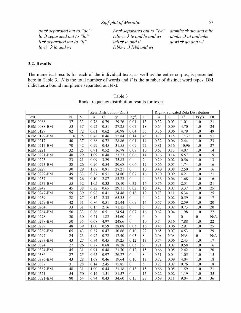
Zipf-plot of Meroitic 57
qo separated out to “qo” lw separated out to “lw” atomhe ato and mhe lo separated out to “lo” telowi te and lo and wi atmhe at and mhe li separated out to “li” teli te and li qowi qo and wi lowi lo and wi lebkwi lebk and wi
3.2. Results The numerical results for each of the individual texts, as well as the entire corpus, is presented here in Table 3. N is the total number of words and V is the number of distinct word types. BM indicates a bound morpheme separated out text.
Table 3 Rank-frequency distribution results for texts
Zeta Distribution (Zipf) Right-Truncated Zeta Distribution Text N V a C χ2 P(χ2) DF a C Χ2 P(χ2) DF REM 0088 37 33 0.78 0.79 29.26 0.01 13 0.32 0.03 1.01 1.0 21 REM 0088-BM 53 37 0.92 0.51 27.25 0.07 18 0.64 0.09 4.70 1.0 24 REM 0129 82 72 0.61 0.62 50.98 0.04 35 0.36 0.06 4.79 1.0 49 REM 0129-BM 116 75 0.78 0.46 52.84 0.14 43 0.73 0.15 17.37 1.0 51 REM 0217 40 37 0.88 0.72 28.86 0.01 14 0.32 0.06 2.44 1.0 23 REM 0217-BM 70 42 0.99 0.45 31.55 0.09 22 0.81 0.16 10.96 1.0 27 REM 0221 32 25 0.91 0.52 16.78 0.08 10 0.63 0.13 4.07 1.0 14 REM 0221-BM 48 29 1.09 0.48 23.23 0.06 14 0.76 0.14 6.57 1.0 19 REM 0223 23 21 0.09 3.29 75.83 0 2 0.29 0.02 0.56 1.0 13 REM 0223-BM 38 26 0.96 0.54 20.68 0.06 12 0.66 0.05 1.74 1.0 16 REM 0229 30 29 1.08 0.91 27.21 0 10 0.40 0.08 2.50 1.0 16 REM 0229-BM 49 33 0.87 0.51 24.80 0.07 16 0.70 0.09 4.21 1.0 21 REM 0237 29 26 0.10 2.87 83.23 0 4 0.36 0.06 1.68 1.0 16 REM 0237-BM 55 32 1.05 0.33 18.10 0.32 16 0.76 0.05 2.51 1.0 21 REM 0247 45 38 0.82 0.65 29.11 0.02 16 0.43 0.07 3.37 1.0 25 REM 0247-BM 59 39 0.98 0.41 24.48 0.18 19 0.73 0.11 6.34 1.0 25 REM 0259 28 27 0.12 2.33 65.35 0 4 0.2 0.02 0.59 1.0 17 REM 0259-BM 42 31 0.86 0.51 21.44 0.09 14 0.57 0.06 2.59 1.0 20 REM 0264 33 31 0.15 2.16 71.15 0 6 0.23 0.02 0.73 1.0 20 REM 0264-BM 50 33 0.86 0.5 24.94 0.07 16 0.62 0.04 1.98 1.0 22 REM 0278 30 30 0.21 1.82 54.60 0 6 0 0 0 0 N/A REM 0278-BM 50 35 0.08 4.97 248.6 0 10 0.7 0.16 7.88 1.0 22 REM 0289 48 39 1.00 0.59 28.08 0.03 16 0.48 0.06 2.91 1.0 25 REM 0289-BM 65 43 0.87 0.47 30.66 0.10 22 0.65 0.07 4.53 1.0 29 REM 0297 24 23 0.92 0.72 17.40 0.03 8 N/A N/A N/A 0 N/A REM 0297-BM 43 27 0.94 0.45 19.25 0.12 13 0.74 0.06 2.43 1.0 17 REM 0324 27 26 0.87 0.68 18.28 0.03 9 0.21 0.02 0.58 1.0 16 REM 0324-BM 45 31 0.91 0.48 21.70 0.12 15 0.66 0.05 2.42 1.0 20 REM 0386 27 25 0.65 0.97 26.27 0 8 0.31 0.04 1.05 1.0 15 REM 0386-BM 43 28 1.08 0.46 19.64 0.10 13 0.72 0.09 4.04 1.0 18 REM 0387 31 28 0.14 2.45 75.85 0 5 0.27 0.02 0.76 1.0 18 REM 0387-BM 48 31 1.00 0.44 21.18 0.13 15 0.66 0.05 1.59 1.0 21 REM 0521 54 50 0.14 1.51 81.57 0 15 0.22 0.02 1.19 1.0 35 REM 0521-BM 80 54 0.94 0.43 34.60 0.15 27 0.69 0.11 9.04 1.0 36

Reginald Smith 58
REM 1003 327 230 0.54 0.23 74.41 1.0 155 0.46 0.03 9.11 1.0 181 REM 1003-BM 360 227 0.64 0.21 74.09 1.0 157 0.58 0.04 15.05 1.0 174 REM 1020 36 31 0.99 0.66 23.65 0.02 12 0.37 0.05 1.79 1.0 20 REM 1020-BM 56 36 0.99 0.45 25.2 0.12 18 0.73 0.10 5.49 1.0 23 REM 1044 (A-D) 435 362 0.45 0.21 93.35 1.0 235 0.40 0.06 26.23 1.0 261 REM 1044(A-D)-BM 449 364 0.48 0.21 95.70 1.0 239 0.43 0.07 30.09 1.0 263 REM 1057 41 38 0.97 0.99 40.41 0 15 0.80 0.45 18.61 0.48 19 REM 1057-BM 61 41 0.92 0.49 29.98 0.09 21 0.69 0.11 6.76 1.0 27 REM 1064 55 48 0.69 0.7 38.37 0.01 21 0.28 0.02 1.36 1.0 34 REM 1064-BM 83 50 0.87 0.39 32.26 0.26 28 0.7 0.05 4.33 1.0 36 Table 4 shows the rank frequency distribution for two of the texts used, REM 1003 (the Amanirenas/Akinidad stela) and REM 1020, this information is provided to allow readers to con-firm the results with their own analysis. Interestingly, REM 1003 had less word types with the bound morphemes removed since many word types in the regular version appear both alone or with one or more types of suffixes, so separated out you are left with less word types.
Table 4 Rank-Frequency Counts: REM 1020 and REM 1003
REM 1020
Normal Bound Morpheme Removed
Rank Frequency Rank Frequency 1 4 1 9 2 2 2 8 3 2 3 4
4-31 1 4 2 5 2 6 2 7-36 1
REM 1003 Normal Bound Morpheme
Removed Rank Frequency Rank Frequency
1 10 1 25 2 8 2 10 3 7 3 8 4 7 4 8 5 5 5 7 6 4 6 7 7 4 7 6
8-19 3 8 5 20-54 2 9 4
55-230 1 10 4 11 4 12 4 13 4 14-24 3 25-61 2 62-226 1

Zipf-plot of Meroitic 59
Below are the plots of the data listed. Figure 1 and Figure 2 show the data plots of one of the larges texts, REM 1003 in both normal and bound morpheme removed versions.
Figure 1. REM 1003 Original Text
Figure 2. REM 1003 Bound Morpheme Separated

Reginald Smith 60
Most texts were funeral texts with a very redundant and standardized structure. The words, wosi (Isis), soreyi (Osiris), terike (begotten of), and tedge (born of) are present in almost all of the funeral texts and this fact is accounted for in their high ranks. Outside of the funeral texts and their repetitious obituaries, only several long stelae remain which seem to be documentaries of the role of the ruler it is dedicated to (ie. Akinidad, Haramadoye, Taneyidamani, etc.). Given this intuitive result, perhaps the language is more accurately represented with the bound morphemes separated since this populates the necessary high frequency words lacking in the first analysis.
Overall, the Meroitic language shows that it behaves like all other human languages in following the Zipf law for word frequency. This starting point allows us to more confidently use further statistical techniques to further understand Meroitic. 4. Conclusion The above analysis indicates that Meroitic, despite being undeciphered, statistically behaves like all other human languages with a word frequency distribution exhibiting power law behavior. Though our texts are very short, the original requirement of a ≈ 1 cannot be maintained. If we use the more realistic version of Zipf´s law, namely the truncation at the right side of the distribution, the value of the parameter a is not characteristic of human language but more probably of the given text or genre.
Modern linguistic theory dictates it is unlikely that one can completely reconstruct a natural language based only on statistical data. However, with words that are already known, perhaps one can use context and other methods to infer currently hidden meanings in the Meroitic texts. This paper serves as a foundation for such work by demonstrating that Meroitic behaves statistically like other languages in adhering to Zipf word frequency distributions. Possible future statistical analysis could use some similarity measure to relate unknown words to current known ones and allow us to perhaps infer the meanings of some unknown words by seeing which known words they are similar to. If such an analysis would even be moderately successful, it would open new doors of analysis both in archaeology and mathematical linguistics.
Acknowledgements The author would like to acknowledge both Laurance Doyle and Richard Lobban whose com-ments were instrumental in finishing this paper. References Ferrer i Cancho, R., Solé, R.V. (2002). Zipf’s Law and Random Texts. Advances in Complex
Systems 5 (1), 1-6. Heyler, Andre (1970). Essai de Transcription Analytique des Textes Meroitiques Isoles.
Meroitic Newsletter 5, 4-8. Heyler, Andre (1974). Meroitic Language and Computers: Problems and Perspectives. In:
Abdalla, A.M. (Editor) Studies in Ancient Languages of the Sudan: 31-39 Khartoum: Khartoum University Press.
Leclant, Jean (1978). The present position in the deciphering of Meroitic script. In: The peopling of ancient Egypt and the deciphering of Meroitic script : proceedings of the symposium held in Cairo from 28 January to 3 February 1974, 107-119. Paris: UNESCO.

Zipf-plot of Meroitic 61
Li, Wentian (1992). Random texts exhibit Zipf's-law-like word frequency distribution. IEEE Transactions in Information Theory 38 (6), 1842-1845.
Lobban, Richard (2004). Historical Dictionary of Ancient and Medieval Nubia. Lanham: Scarecrow.
Mandelbrot, Benoit (1953). An informational theory of the statistical structure of language. In: Willis Jackson (ed.), Communication Theory: 486-502. London: Butterworths Scientific Publishing.
McCowan, B., Hanser, S., Doyle L.R. (1999). Quantitative tools for comparing animal com-munication systems: information theory applied to bottlenose dolphin whistle repertoires. Animal Behaviour 57, 409-419.
McCowan, B., Doyle, L.R., Jenkins, J.M., Hanser (2005). The Appropriate Use of Zipf's Law in Animal Communications Studies. Animal Behaviour 68, F1-F7.
Miller, G. A. (1957). Some effects of intermittent silence. American Journal of Psychology 70, 311-314.
Newman, M.E.J. (2005). Power laws, Pareto distributions and Zipf’s law. Contemporary Phys-ics 46, 323-351.
Rilly, Claude (2004). The Linguistic Position of Meroitic. ARKAMANI Sudan Journal of Ar-chaeology and Anthropology. [http://www.arkamani.org/arkamani-library/meroitic/rilly. htm].
Török, László (1997). The Kingdom of Kush: Handbook of the Napatan-Meroitic Civilization. London: Brill.
Zipf, George K. (1948). Human behavior and the principle of least effort; an introduction to human ecology. Cambridge: Addison-Wesley.

Glottometrics 15, 2007, 62-70
A psycholinguistic application of synergetic linguistics
Reinhard Köhler, Trier Reinhard Rapp, Mainz/Tarragona
Abstract: The paper presents a new attempt to analyse the relationship between word familiarity and word frequency within the framework of synergetic linguistics. Whereas in psychology it is customary to apply correlational analyses to such questions the current paper sets up a functional model and tests it on empirical data from two large corpora and a psycholinguistic database. Keywords: psycholinguistics, word familiarity, word frequency, synergeticlinguistics Introduction The modeling paradigm of synergetic linguistics (see Köhler 1986, 1990, 2005) is well suited to interdisciplinary work and to the creation of models which allow the interconnection of several disciplines. By looking at two quantities, word frequency and word familiarity, the ex-ample considered here shows how an interface between the two neighboring disciplines of psychology and linguistics can be created in this way.
Rapp (2005) considered the relationship between the occurrence frequencies of words in a corpus and the subjective judgments of their familiarity provided by human subjects. The aim of this study was to provide evidence that word occurrences are observed by human per-ception, and that the frequencies of words are stored in memory. It is argued that this could be demonstrated if it were the case that, when subjects are asked questions related to word fre-quencies, the answers tend to be correct.
However, in such experiments it turns out that it is almost impossible for subjects to give correct estimates of absolute values of word frequencies. Much better results are achieved, however, if judgments of word familiarity are elicited. This can be measured using, for ex-ample, a grade scale of 1 to 7. Psychologists have conducted such experiments on a large scale, and their results were compared with word frequencies as found in balanced corpora. The simplifying assumption was made that the word frequencies as obtained from the corpora are representative of the language environment of the test subjects.
In the study it was shown that there is a strong correlation of r = 0.75 between the corpus frequencies of words and the familiarity ratings for those words provided by test subjects. Similar investigations by other authors led to similar results. Underwood et al. (1965) report a correlation of r = 0.85, and Kreuz (1987) a correlation of r = 0.75. By comparison, the correlations of familiarity ratings between different groups of test subjects were only slightly higher than this (between 0.77 and 0.88). This provides some evidence in favor of the hyp-othesis given above, namely that word frequencies are stored in human memory. However, it should not be forgotten that a high correlation is not sufficient to imply causality.
Also, correlation analysis, although a standard method in psychology, is a weak and some-times misleading method for describing relationships of the kind considered here, which are nonlinear. This is because correlations can only take the linear parts of a relationship into ac-
A psycholinguistic application of synergetic linguistics 63
count, and even those only as the strength of a tendency. To avoid these drawbacks it makes sense to conduct a functional analysis, for example a nonlinear regression.
Therefore, this study attempts to theoretically derive the relationship between the corpus frequencies of words and their familiarity judgments as provided by test subject, as a func-tional dependency in the framework of synergetic linguistics. The resulting model is empir-ically tested using the same data as was used by Rapp (2005).
Data Our source of familiarity judgments from test subjects was the online version of the MRC1 Psycholinguistic Database (Coltheart, 1981a; 1981b), for which Craig Clark has developed a user friendly and flexible web interface.2 According to Wilson (1988) the MRC database provides familiarity estimates for 9392 entries. Table 1 shows a few examples. However, these 9392 entries correspond to only 4920 words, as in the MRC database an entry is defined as the combination of a word with its part of speech. Therefore, ambiguous words that can occur as different parts of speech are counted more than once.
The familiarity estimates are based on judgments from test subjects who were asked to assign to each word a familiarity value on the usual scale between 1 (for a word unknown to a subject) and 7 (for a very familiar word from everyday language). Collections of such fam-iliarity judgments are usually referred to as familiarity norms. In order to provide estimates for as many words as possible, familiarity judgments from three different experiments were included in the MRC database. The experiment conducted by Toglia & Battig (1978) con-tributed 2854 words, the experiment by Gilhooly and Logie (1980) contributed 1944 words, and Paivio et al. (1968) provided an unpublished expanded version of their data consisting of 2310 words. As there is some overlap in vocabulary, Table 2 lists how many words the three studies have in common. It also shows the high correlations of the familiarity ratings between the three groups of test subjects.
When creating the MRC psycholinguistic database, on the basis of these high correlat-ions Coltheart (1981a) decided to merge the three studies by averaging the values correspond-ing to the same words. Beforehand he had adjusted the overall means and standard deviations of the three studies. In order to not pretend unjustifiable high accuracies of the merged familiarity judgments, Coltheart decided to round the floating point numbers that were the result of the averaging process after two decimals. He then multiplied the resulting values by 100 so that the range of familiarity judgments in the MRC database is not between 1 and 7, but between 100 and 700, as stated by Wilson (1988). However, to be more precise, it must be noted that the process of adjusting the means and standard deviations of the three underlying studies led to some distortion of this range, so that actually a few values below 100 can be observed.
1 MRC stands for the Medical Research Council, the funding organisation for the project. 2 http://www.psy.uwa.edu.au/mrcdatabase/uwa_mrc.htm

R. Köhler, R. Rapp 64
Table 1 The 10 words with the highest and the lowest familiarities in the MRC Psycholinguistic
Database together with their frequency in the Brown Corpus (words with a corpus frequency of zero are not included).
WORD FAM. FREQ. WORD FAM. FREQ.
BREAKFAST 657 53 LOQUACITY 144 1 AFTERNOON 655 106 MIEN 143 1 CLOTHES 652 89 YUCCA 136 1 BEDROOM 646 52 BURGHER 133 1 DAD 646 15 PAEAN 133 2 GIRL 645 220 OBELISK 131 6 RADIO 644 120 PLENIPOTENTIARY 128 1 BOOK 643 193 TAPIS 118 1 NEWSPAPER 641 65 METIS 101 1 WATER 641 442 VERDANT 98 1
Table 2
Vocabulary overlap and correlations between three familiarity norms according to Coltheart (1981a).
FAMILIARITY NORMS COMMON WORDS CORRELATION
Toglia & Battig / Gilhoooly & Logie 597 0.77 Paivio et al. / Gilhooly & Logie 427 0.88 Toglia & Battig / Paivio et al. 882 0.88
Estimates of the word frequencies in everyday language as experienced by the test subjects were derived from two balanced corpora of English which, given the impossibility of a per-fect solution, seemed best suited to model the language environment of an average subject. These were the Brown Corpus (Francis & Kučera 1989), which comprises about 1 million words, and the British National Corpus (BNC; Burnard & Aston 1998) consisting of about 100 million words. The database uses uppercase letters only (see Table 1), a reflection of the time of its creation. Therefore, before counting the corpus frequencies of words we pre-processed the two corpora to capitalise them throughout. Although occasionally this may add some ambiguity, we do not expect a major impact on the word counts of the particular vocabulary we are interested in. The Model If, in analogy to other relationships between properties of words, it is assumed that the familiarity of a word shows a relative increase as the frequency of perception of that word grows, then this can be expressed as a differential equation:
xB
yy=
' , (1)
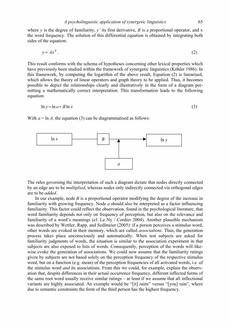
A psycholinguistic application of synergetic linguistics 65
where y is the degree of familiarity, y’ its first derivative, B is a proportional operator, and x the word frequency. The solution of this differential equation is obtained by integrating both sides of the equation: . (2) BAxy = This result conforms with the schema of hypotheses concerning other lexical properties which have previously been studied within the framework of synergetic linguistics (Köhler 1986). In this framework, by computing the logarithm of the above result, Equation (2) is linearised, which allows the theory of linear operators and graph theory to be applied. Thus, it becomes possible to depict the relationships clearly and illustratively in the form of a diagram per-mitting a mathematically correct interpretation. This transformation leads to the following equation:
ln (3) xBay lnln += With a = ln A, the equation (3) can be diagrammatised as follows:
ln y B
a
ln x The rules governing the interpretation of such a diagram dictate that nodes directly connected by an edge are to be multiplied, whereas nodes only indirectly connected via orthogonal edges are to be added.
In our example, node B is a proportional operator modifying the degree of the increase in familiarity with growing frequency. Node a should also be interpreted as a factor influencing familiarity. This factor could reflect the observation, found in the psychological literature, that word familiarity depends not only on frequency of perception, but also on the relevance and familiarity of a word’s meanings (cf. Le Ny / Cordier 2004). Another plausible mechanism was described by Wettler, Rapp, and Sedlmeier (2005): if a person perceives a stimulus word, other words are evoked in their memory, which are called associations. Thus, the generation process takes place unconsciously and automatically. When test subjects are asked for familiarity judgments of words, the situation is similar to the association experiment in that subjects are also exposed to lists of words. Consequently, perception of the words will like-wise evoke the generation of associations. We could now assume that the familiarity ratings given by subjects are not based solely on the perception frequency of the respective stimulus word, but on a function (e.g. mean) of the perception frequencies of all activated words, i.e. of the stimulus word and its associations. From this we could, for example, explain the observ-ation that, despite differences in their actual occurrence frequency, different inflected forms of the same root word usually receive similar ratings – at least if we assume that all inflectional variants are highly associated. An example would be “[it] rains” versus “[you] rain”, where due to semantic constraints the form of the third person has the highest frequency.

R. Köhler, R. Rapp 66
This partial hypothesis could be tested empirically in several ways. One possibility would be to use lemma frequencies instead of word counts, or to use weighted means of the inflect-ional forms relating to the same root form (which, however, also requires lemmatization of the corpus). Another possibility would be the comparison of similar experiments based on a number of different languages, some highly inflectional, others less so. However, this has not been done yet and will be left for future investigation. On the other hand it should be noted that the synergetic modelling and a test of our initial hypothesis do not depend on the inter-pretation of the factor a.
If in our diagram we replace x with the frequency and y with the familiarity, and if we take the necessity of logarithmic transformation of these variables into account, we obtain a new diagram that is more specific with respect to our particular case:
In contrast to models from previous studies, which considered purely linguistic relationships, here we need to remember that the range of values of the variable familiarity has a lower and an upper limit. Whereas the linguistic variable frequency has only a lower limit of x = 1, the familiarity measure has an upper limit of V = 700 in theory, but of V = 600 in our practical data. For this reason we modify the model as follows:
L-max L-familiarity
-B
a
L-frequency
a
L-familiarity BL-frequency
L-max denotes the logarithm of the upper limit V. The operator B needs to be negative so that the structure of the model is in accordance with equation (4)
ln (4) )ln(lnln xBaVy +−= or with the reverse transformation of (4) into the non-linear equation (5):
BAxVy= . (5)
With regard to the empirical test, we need to take into account the fact that large values of x (frequency), which can occur when very large corpora are used, may in practice lead to

A psycholinguistic application of synergetic linguistics 67
division by zero errors. This is because of the exponent B, which quickly lets the inverse of x get so close to zero that, given the limited accuracy of standard computations, it may not be possible to distinguish it from zero. To avoid this problem we add 1 in the denominator which does not impair the validity of the model:
BAxVy
+=
1. (6)
Testing the Model The adaptation of the model (6) to the data of the Brown Corpus leads (with V being empirically determined to be 629) to the following values of our parameters: A = 0.6923, B = -0.3649. With a determination coefficient of R2 = 0.61 this result does not at first glance look very convincing. However, as the variance of the familiarities is very high, this low value of R2 is still in agreement with the model. Note that the variance is caused by discrepancies in the familiarity judgments of the test subjects. However, Figure 1 shows that the trend of the data is well predicted by the model.
Figure 1. Fitting the model (6) to the data from the Brown Corpus:
familiarity as a function of frequency This is confirmed by an experiment where the data was smoothed using moving averages over an interval of 30 (see Figure 2). The empirical maximum of this curve is V = 584. The corresponding values of the parameters are A = 2.880, B = -0.9273, and R2 = 0.92, which is a convincing result.

R. Köhler, R. Rapp 68
Figure 2. Fitting the model (6) to the smoothed data from the Brown Corpus:
familiarity as a function of frequency Another test of the model was conducted using frequency data from the BNC, which, as stated previously, is 100 times larger than the Brown Corpus. For the same reasons as before, moving averages with an interval size of 30 were again used. From these data we obtained, with a V of 632, the following parameters, which indicate an excellent fit: A = 3.11, B = -0.3428, and R2 = 0.98 (see Figure 3).
Figure 3. Fitting the model (6) to the smoothed data from the BNC:
familiarity as a function of frequency

A psycholinguistic application of synergetic linguistics 69
Summary and Prospects Previous studies dealing with the relationship between word frequency and word familiarity judgments were usually based on a correlational analysis, which is the standard procedure in psychology in such cases. However, in this way only the linear component of a relationship can be taken into account, which is a clear drawback. By contrast, the present study shows, for two different corpora, a convincing functional relationship which takes into account the substantial non-linearity depicted in Figures 1 to 3. This means that predictions derived from the new model should be a considerable improvement over the predictions of previous models. It would be of interest to confirm whether the functional relationship discovered here holds true for languages other than English. A problem is that most familiarity norms were compiled for English, with little data available for other languages. Acknowledgment Part of this work was supported by the European Union in the framework of a Marie Curie Intra-European Fellowship. References Burnard, Lou; Aston, Guy (1998), The BNC Handbook: Exploring the British National
Corpus with Sara. Edinburgh University Press. Coltheart, Max (1981a), MRC Psycholinguistic Database User Manual: Version 1.
http://www.psych.rl.ac.uk/User_Manual_v1_0.html Coltheart, Max (1981b), The MRC Psycholinguistic Database. Quarterly Journal of
Experimental Psychology, 33A, 497–505. Francis, W. Nelson; Kucera, Henry (1989), Manual of Information to Accompany a
Standard Corpus of Present-Day Edited American English, for Use with Digital Computers. Providence, R.I.: Brown University, Department of Linguistics.
Gilhooly, Kenneth J.; Logie, Robert H. (1980), Age of acquisition, imagery, concreteness, familiarity and ambiguity measures for 1944 words. Behaviour Research Methods and Instrumentation 12, 395–427.
Köhler, Reinhard (1986), Zur linguistischen Synergetik. Struktur und Dynamik der Lexik. Bochum: Brockmeyer.
Köhler, Reinhard (1990), Elemente der synergetischen Linguistik. In: Glottometrika 12 (ed. Rolf Hammerl), 179-188. Bochum: Brockmeyer.
Köhler, Reinhard (2005), Synergetic Linguistics. In: Köhler, Reinhard, Altmann, Gabriel, Piotrowski, Rajmund G. [ed.]: Quantitative Linguistik. Ein internationales Handbuch. Quantitative Linguistics. An International Handbook: 760-775. (= HSK27) Berlin, New York: de Gruyter..
Kreuz, Roger J. (1987), The subjective familiarity of English homophones. Memory & Cognition 15, 154–168.
Le Ny, Jean-François; Cordier, Françoise (2004), Contribution of word meaning and components of familiarity to lexical decision: A study with pseudowords constructed from words with known or unknown meaning. In: Current Psychology Letters 12, Vol.1 (http://cpl.revues.org/document416.html)

R. Köhler, R. Rapp 70
Paivio, Allan; Yuille, John C.; Madigan, Stephen A. (1968), Concreteness, imagery and meaningfulness values for 925 words. Journal of Experimental Psychology Monograph Supplement, 76 (3, part 2).
Rapp, Reinhard (2005), On the relationship between word frequency and word familiarity. In: Benhard Fisseni; Hans-Christian Schmitz; Bernhard Schröder; Petra Wagner (Hg.): Sprachtechnologie, mobile Kommunikation und linguistische Ressourcen. Beiträge zur GLDV-Tagung 2005 in Bonn. Frankfurt: Peter Lang. 249–263.
Toglia, Michael P.; Battig, William F. (1978), Handbook of Semantic Word Norms. New York: Erlbaum.
Underwood, Benton J.; Ekstrand, Bruce R.; Keppel, Geoffrey (1965), An analysis of intralist similarity in verbal learning with experiments on conceptual similarity. Journal of Verbal Learning and Verbal Behavior, 4, 447–462.
Wettler, Manfred; Rapp, Reinhard; Sedlmeier, Peter (2005). Free word associations correspond to contiguities between words in texts. Journal of Quantitative Linguistics 12 (2), 111–122.
Wilson, Michael D. (1988), The MRC Psycholinguistic Database: Machine Readable Dictionary, Version 2. Behavior Research Methods, Instruments, & Computers 20, 6–11.

Glottometrics 15, 2007, 71-81
Writer´s view of text generation
Ioan-Iovitz Popescu, Bucharest1 Gabriel Altmann, Lüdenscheid
Abstract: Generally, a “writer’s view”, defined by the angle between the ends of the word rank-fre-quency distribution, as seen from the h-point, should be limited in the interval [π/2, π]. However, as shown in the present paper with 176 texts from 20 languages, actually the lower limit appears to be the golden number φ = 1.618... , rather than π/2 = 1.57... Keywords: h-point, rank-frequency distributions, golden section The writer of a text abides by some mechanisms of writing. Writing and speaking is a human activity performed according to some rules, habits or laws. Some of the mechanisms are conscious, other ones are unconscious, the writers need not even be aware of their existence. What is conscious, is the given language, its grammar, the contents of the text, the approx-imate length of the text and, after some thinking, the order of events in which the narrative must be presented, etc. The writer can control consciously the sentence length, the choice of words and some other properties, but he cannot control consciously everything. Some of the unconscious processes may sometimes become conscious, especially when one speaks an artificially learned language. But even in a foreign language we must suppose the existence of unconscious control of different processes.
Here we shall examine only the process of increasing word frequencies in text and building the rank-frequency distribution. As the text increases in length, new words are added occurring at first just once (new types), or some words are repeated getting higher frequency of occurrence. Predictions about a new occurrence of a certain word can be made only prob-abilistically and are not very reliable. While both the words at lower ranks continuously in-crease their frequency and new words (hapax legomena) are added, the beginning of the frequency curve increases vertically and the tail of the curve increases horizontally. Besides, the words at not extreme ranks steadily change their (rank) positions, thus the frequency curve seems to be in a steady flux. Nevertheless, there are some more solid entities in rank-fre-quencies of words conserving their properties in spite of the steady motion accompanying the increase of text. We mention here the distribution itself – being of Zipfian type or its gener-alizations; Ord’s criteria – being characteristic for languages; and the type-token curves, etc. (cf. Popescu et al. 2007). Other properties arise through self-organization, e.g. building of bin-ary runs of F-segments in long sentences (cf. Uhlířová 2007).
Here we shall report a peculiar convergence property of the rank-frequency distribution, f = f(r), by observing the development of the so-called h-point during the increase of text length. As is known (s. Popescu 2006; Popescu, Altmann 2006; Popescu et al. 2007), the h-point is defined as the point at which r = f(r), i.e. where the rank is equal to frequency. As a rule, the actual rank-frequency distributions are discrete and this is why sometimes the h-point is situated between two ranks; but its exact value can easily be computed in different ways. In graphical terms, the fitted graph of f(r) has the h-point in common with the line y = x. An analytical method consists in the best fitting with a Zipf distribution, ( ) / af r c r= (with a and 1 Address correspondence to: [email protected]
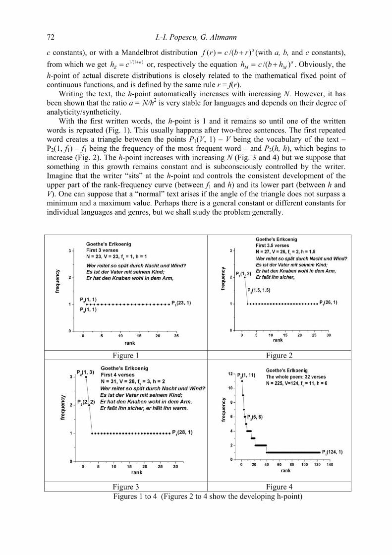
I.-I. Popescu, G. Altmann 72
c constants), or with a Mandelbrot distribution ( ) /( )af r c b r= + (with a, b, and c constants), from which we get or, respectively the equation h c . Obviously, the h-point of actual discrete distributions is closely related to the mathematical fixed point of continuous functions, and is defined by the same rule r = f(r).
1/(1 )aZh c += /( )a
M b h= + M
Writing the text, the h-point automatically increases with increasing N. However, it has been shown that the ratio a = N/h2 is very stable for languages and depends on their degree of analyticity/syntheticity.
With the first written words, the h-point is 1 and it remains so until one of the written words is repeated (Fig. 1). This usually happens after two-three sentences. The first repeated word creates a triangle between the points P1(V, 1) – V being the vocabulary of the text – P2(1, f1) – f1 being the frequency of the most frequent word – and P3(h, h), which begins to increase (Fig. 2). The h-point increases with increasing N (Fig. 3 and 4) but we suppose that something in this growth remains constant and is subconsciously controlled by the writer. Imagine that the writer “sits” at the h-point and controls the consistent development of the upper part of the rank-frequency curve (between f1 and h) and its lower part (between h and V). One can suppose that a “normal” text arises if the angle of the triangle does not surpass a minimum and a maximum value. Perhaps there is a general constant or different constants for individual languages and genres, but we shall study the problem generally.
Figure 1 Figure 2
Figure 3 Figure 4 Figures 1 to 4 (Figures 2 to 4 show the developing h-point)

Writer´s view of text generation 73
Let us consider a word rank-frequency distribution represented, as usually (see Figure 4), in a Cartesian Oxy system of coordinates, Ox for ranks (with the maximum value V at the point P1) and Oy for frequencies (with the maximum value f1 at the point P2). Let us also have the h-point located at the point P3. To summarize, we have the three characteristic points of the distribution given by their coordinates as follows:
P1 (V, 1) P2 (1, f1) P3 (h, h)
We will consider the angle seen from the h-point P3 and formed by the directions towards
the distribution end P1 and top P2. In other words, we want an expression of the angle between the following two vectors:
(a) the vector a (ax, ay), directed from the h-point P3 towards the distribution top P2, having the components
ax = - h ay = f1 - h
and the absolute value (modulus) (1) a = (ax
2 + ay2)1/2 = (h2 + (f1 – h)2)1/2
(b) the vector b (bx, by), directed from the h-point P3 towards the distribution end P1,
having the components
bx = V - h by = - h
and the absolute value (modulus) (2) b = (bx
2 + by2)1/2 = ((V – h)2 + h2)1/2
In order to get the angle between the above vectors a and b we shall use the well known
dot product formula of vector calculus (3) cos α = a.b/ab where (4) a.b = axbx + ayby that is
(5) 2 2 1/2 2 2 1/2
cos =
[( + ) ][( ) ]x x y y
x y x y
a b a ba a b b
α+
+
which, in our particular case, becomes
(6) 12 2 1/ 2 2
1
[ ( ) ( )]cos[ ( ) ] [ ( ) ]
h f h h V hh f h h V h
α − − + −=
+ − + − 2 1/ 2

I.-I. Popescu, G. Altmann 74
As expected, all numerical cosine values are negative because the corresponding angles are located in the second quadrant (from π/2 to π radians, respectively from 90 to 180 degrees). Let us illustrate the computation for a text having length N = 761, V = 400, h =10 and f1 = 40. Inserting these numbers in (6) we obtain
2 2 1/ 2 2 2 1/ 2
[10(40 10) 10(400 10)]cos 0.3404[10 (40 10) ] [10 (400 10) ]
α − − + −= =
+ − + −−
hence α = 1.9182 radians.
In order to study the behavior of the angle α in radians, which we call “writer´s view”, we used the data published in Popescu et al. (2007) containing 176 texts in 20 languages as presented in Table 1. Here B = Bulgarian, Cz = Czech, E = English, G = German, H = Hun-garian, Hw = Hawaiian, In = Indonesian, I = Italian, Kn = Kannada, Lt = Latin, Lk = Lakota, M = Maori, Mq = Marquesan, Mr = Marathi, R = Romanian, Rt = Rarotongan, Ru = Russian, Sl = Slovenian, Sm = Samoan, T = Tagalog. Ordering the table according to increasing text length (N) we obtained a surprising result: The angle called “writer´s view” converges to the golden section known from several arts, different domains of aesthetics and sciences, namely to
1 5 1.6180
2ϕ += = …,
as can be seen in Table 1 and in Figure 5.
Table 1 The development of “writer’s view” in increasing text size (176 texts from 20 languages)
Text ID N V f(1) h cos α α rad
G 14 184 129 10 5 -0.735 2.3965Lk 04 219 116 18 6 -0.4953 2.0889G 17 225 124 11 6 -0.7997 2.4977G 12 251 169 14 6 -0.629 2.2511G 07 263 169 17 5 -0.4126 1.9961B 08 268 179 10 6 -0.8508 2.5883
Hw 01 282 104 19 7 -0.5647 2.1709In 04 343 213 11 5 -0.6585 2.2896Lk 01 345 174 20 8 -0.5941 2.207In 03 347 194 14 6 -0.6252 2.2462B 02 352 201 13 8 -0.8692 2.6244In 02 373 209 18 7 -0.5658 2.1722In 01 376 221 16 6 -0.5382 2.1391H 03 403 291 48 4 -0.1044 1.6754B 05 406 238 19 7 -0.5298 2.1292H 05 413 290 32 6 -0.2454 1.8187In 05 414 188 16 8 -0.7378 2.4006

Writer´s view of text generation 75
Sm 05 447 124 39 11 -0.4541 2.0422Mq 02 457 150 42 10 -0.3655 1.945Cz 09 460 259 30 6 -0.2655 1.8395G 13 460 253 19 8 -0.6143 2.2322G 11 468 297 18 7 -0.5571 2.1617G 10 480 301 18 7 -0.5568 2.1613B 04 483 286 21 8 -0.5484 2.1512G 03 500 281 33 8 -0.3325 1.9098B 03 515 285 15 9 -0.8497 2.5862G 16 518 292 16 8 -0.7267 2.3844Cz 04 522 323 27 7 -0.3512 1.9296G 04 545 269 32 8 -0.3451 1.9232G 06 545 326 30 8 -0.3653 1.9447B 09 550 313 20 9 -0.6559 2.2861B 10 556 317 26 7 -0.3668 1.9464B 07 557 324 19 8 -0.6085 2.2249G 05 559 332 30 8 -0.3648 1.9443G 15 593 378 16 8 -0.7222 2.3778
Sm 03 617 140 45 13 -0.4688 2.0587Rt 04 625 181 49 11 -0.3395 1.9172G 09 653 379 30 9 -0.4162 2.0000Cz 08 677 389 31 8 -0.3483 1.9265B 06 687 388 28 9 -0.4494 2.0369R 06 695 432 30 10 -0.4683 2.0581
Sm 04 736 153 78 12 -0.2617 1.8356Ru 01 753 422 31 8 -0.3467 1.9249Sl 01 756 457 47 9 -0.2500 1.8234B 01 761 400 40 10 -0.3404 1.9182Lk 03 809 272 62 12 -0.2780 1.8525Lt 06 829 609 19 7 -0.5139 2.1105G 02 845 361 48 9 -0.2497 1.8232Rt 02 845 214 69 13 -0.2885 1.8635I 03 854 483 64 10 -0.2028 1.775
Rt 03 892 207 66 13 -0.3026 1.8782H 04 936 609 76 7 -0.1125 1.6835G 08 965 509 39 11 -0.3861 1.9672Rt 01 968 223 111 14 -0.2087 1.781Cz 02 984 543 56 11 -0.2575 1.8312Cz 05 999 556 84 9 -0.1355 1.7067R 05 1032 567 46 11 -0.3186 1.8951Cz 01 1044 638 58 9 -0.1947 1.7668

I.-I. Popescu, G. Altmann 76
Kn 004 1050 720 23 7 -0.4098 1.993Rt 05 1059 197 74 15 -0.3252 1.902G 01 1095 530 83 12 -0.1894 1.7614I 05 1129 512 42 12 -0.3936 1.9753
Cz 10 1156 638 50 11 -0.2883 1.8632Sm 02 1171 222 103 15 -0.2388 1.812M 02 1175 277 127 15 -0.1892 1.7611R 03 1264 719 65 12 -0.2373 1.8104R 04 1284 729 49 10 -0.2618 1.8357H 02 1288 789 130 8 -0.0757 1.6465M 04 1289 326 137 15 -0.1697 1.7413
Kn 013 1302 807 35 10 -0.383 1.9638Lt 05 1354 909 33 8 -0.3132 1.8894Sl 02 1371 603 66 13 -0.2596 1.8334M 03 1434 277 128 17 -0.2156 1.7881Sm 01 1487 267 159 17 -0.186 1.7578Mq 03 1509 301 218 14 -0.117 1.6881T 01 1551 611 89 14 -0.2065 1.7788Cz 06 1612 840 106 13 -0.154 1.7254Lk 02 1633 479 124 17 -0.1931 1.7651R 01 1738 843 62 14 -0.2962 1.8715T 02 1827 720 107 15 -0.1819 1.7537
Hw 02 1829 257 121 21 -0.2914 1.8665Mr 035 1862 1115 29 11 -0.5299 2.1293Sl 03 1966 907 102 13 -0.1589 1.7304Cz 07 2014 862 134 15 -0.1426 1.7139H 01 2044 1079 225 12 -0.0675 1.6383T 03 2054 645 128 19 -0.2015 1.7737M 01 2062 398 152 18 -0.1799 1.7517R 02 2279 1179 110 16 -0.1813 1.7531E 01 2330 939 126 16 -0.1611 1.7326
Mq 01 2330 289 247 22 -0.1787 1.7505Ru 02 2595 1240 138 16 -0.143 1.7143Cz 03 2858 1274 182 19 -0.1308 1.702
Mr 002 2922 1186 73 18 -0.3256 1.9025Mr 149 2946 1547 47 12 -0.3317 1.9089
E 02 2971 1017 168 22 -0.1708 1.7425Mr 001 2998 1555 75 14 -0.2325 1.8055Mr 007 3162 1262 80 16 -0.255 1.8286Kn 003 3188 1833 74 13 -0.2154 1.7879
E 03 3247 1001 229 19 -0.1094 1.6804
Writer´s view of text generation 77
I 04 3258 1237 118 21 -0.2284 1.8013Lt 01 3311 2211 133 12 -0.1041 1.6751
Mr 293 3337 2006 41 13 -0.427 2.012Mr 043 3356 1962 44 16 -0.5033 2.0982Mr 150 3372 1523 64 16 -0.3263 1.9032Mr 029 3424 1412 28 17 -0.8461 2.5795Mr 034 3489 1865 40 17 -0.6018 2.2165Sl 04 3491 1102 328 21 -0.0876 1.6585
Hw 03 3507 521 277 26 -0.1551 1.7265Mr 052 3549 1628 89 17 -0.24 1.8132Mr 154 3601 1719 68 17 -0.3257 1.9025M 05 3620 514 234 26 -0.1767 1.7484
Mr 016 3642 1831 63 18 -0.3806 1.9612Mr 006 3735 1503 120 19 -0.1974 1.7695Mr 294 3825 1931 85 17 -0.2511 1.8247Mr 296 3836 1970 92 18 -0.2453 1.8186Mr 021 3846 1793 58 20 -0.4757 2.0666Ru 03 3853 1792 144 21 -0.18 1.7518
Mr 020 3943 1825 62 19 -0.4138 1.9974Mr 291 3954 1957 86 18 -0.2649 1.8389Lt 02 4010 2334 190 18 -0.1118 1.6828
Mr 290 4025 2319 42 17 -0.5684 2.1754Mr 288 4060 2079 84 17 -0.2539 1.8275Mr 018 4062 1788 126 20 -0.1965 1.7686Mr 038 4078 1607 66 20 -0.4103 1.9935Mr 022 4099 1703 142 21 -0.1833 1.7551Mr 027 4128 1400 92 21 -0.2982 1.8736Mr 003 4140 1731 68 20 -0.3954 1.9773Kn 012 4141 1842 58 19 -0.4473 2.0346Mr 023 4142 1872 72 20 -0.369 1.9488Mr 026 4146 2038 84 19 -0.2896 1.8646Mr 017 4170 1853 67 19 -0.3777 1.9581Mr 046 4186 1458 68 20 -0.3974 1.9795Mr 036 4205 2070 96 19 -0.2486 1.822Mr 024 4255 1731 80 20 -0.3273 1.9042Lt 04 4285 1910 99 20 -0.2557 1.8293
Kn 017 4316 2122 122 18 -0.179 1.7507Mr 033 4339 2217 71 19 -0.3513 1.9298Kn 011 4541 2516 63 17 -0.353 1.9316Mr 297 4605 2278 88 18 -0.2567 1.8305
E 04 4622 1232 366 23 -0.0859 1.6568

I.-I. Popescu, G. Altmann 78
Mr 015 4693 1947 136 21 -0.1904 1.7623Kn 016 4735 2356 93 18 -0.2409 1.814
E 05 4760 1495 297 26 -0.1131 1.6841Mr 292 4765 2197 88 19 -0.2739 1.8482Mr 289 4831 2312 112 19 -0.2083 1.7806Mr 151 4843 1702 192 23 -0.1484 1.7198
E 06 4862 1176 460 24 -0.0757 1.6466Kn 005 4869 2477 101 16 -0.1914 1.7634Mr 295 4895 2322 97 20 -0.2598 1.8336Lt 03 4931 2703 103 19 -0.2275 1.8003
Mr 005 4957 2029 172 19 -0.1326 1.7038E 07 5004 1597 237 25 -0.1329 1.7041E 08 5083 985 466 26 -0.086 1.6569
Mr 031 5105 2617 91 21 -0.2951 1.8703Mr 028 5191 2386 86 23 -0.3521 1.9306Mr 032 5195 2382 98 23 -0.3025 1.8781Mr 040 5218 2877 81 21 -0.3373 1.9148Kn 006 5231 2433 74 20 -0.3551 1.9338Mr 010 5394 1650 217 27 -0.1571 1.7286Mr 008 5477 1807 190 27 -0.1784 1.7501Mr 030 5504 2911 86 20 -0.2966 1.8719Sl 05 5588 2223 193 25 -0.1584 1.7299E 09 5701 1574 342 29 -0.1109 1.682
Ru 04 6025 2536 228 25 -0.1321 1.7033I 02 6064 2203 257 25 -0.1185 1.6896
Mr 009 6206 2387 93 26 -0.372 1.952E 10 6246 1333 546 28 -0.0754 1.6463
Mr 004 6304 2451 314 24 -0.0923 1.6633Hw 05 7620 680 416 38 -0.1586 1.7301Hw 04 7892 744 535 38 -0.1297 1.7009E 11 8193 1669 622 32 -0.0737 1.6445E 12 9088 1825 617 39 -0.0891 1.66E 13 11265 1659 780 41 -0.0807 1.6516I 01 11760 3667 388 37 -0.115 1.686
Hw 06 12356 1039 901 44 -0.0953 1.6663Ru 05 17205 6073 701 41 -0.0688 1.6396
In Figure 5 we see that some texts approximate this value even if they are short, but in any case, long texts tend to it. For instance, the latter case is best demonstrated by Goethe’s Faust as shown in the table below

Writer´s view of text generation 79
Text N V f(1) h cos α α rad Faust 1. 30625 6303 918 64 -0.0850 1.6559 Faust 1. and 2. 75050 13341 2089 90 -0.0518 1.6226
This is, perhaps, the way how to attain harmonic proportions in texts. It may be expected that further texts with N ≈ 2500 had filled the gap in Figure 5 between the two branches of the points following most probably a power curve.
Figure 5. Illustrating the dependence of the “writer’s view” α radians in terms of the text length N for 176 texts in 20 languages. All data lay within the interval φ = 1.618... to π = 3.14...
The theoretical upper angle is π = 3.14..., however, the actual boundary is not precisely known. Many shorter texts (e.g. poems) must be analysed in order to venture a well grounded statement. One example is given in continuation with cumulative sequences from Goethe’s Erlkönig indicating for the corresponding upper boundary an average value of about 3 (Table 2).
Though we believe that the golden section is present in texts in some way and can be found by different methods, the fact that the rank-frequency distribution and its h-point can make it at least visible, is a good argument for further study of word frequencies.

I.-I. Popescu, G. Altmann 80
Table 2 Development of α rad in Goethe´s Erlkönig
Goethe’s Erlkönig N V f(1) h cos α α rad first 10 words 10 10 1 1 -0.9939 3.0309 first 20 words 20 20 1 1 -0.9986 3.0890 first 30 words 30 27 3 2 -0.9272 2.7578 first 60 words 60 45 3 3 -0.9975 3.0703 first 100 words 100 69 4 4 -0.9981 3.0801 first 140 words 140 88 7 5 -0.9491 2.8213 first 220 words 220 122 11 6 -0.8003 2.4985
The texts in Table 1 are all of moderate length, allowing us to suppose that they were
written “in one go”. It is known that several writers were able to write a book in one day. Practically, longer texts are mixtures of texts even if they were written by the same author. The smooth process of writing is interrupted in many places and a new “vocabulary regime” can distort all ratios (e.g. TTR, the α angle, the thematic concentration etc.). Hence their investigation is not very prolific. Nevertheless, we ventured an experiment and took some very long texts, even translations (which are on many grounds forbidden in linguistics) and brought them to a common statement about the mean of the α radian. As individual texts they have no expressiveness – because they are mixed – but representing a statistical sample they can tell us something about the unweighted mean of the sample. In Table 3 we show some randomly chosen well known mixtures. Though with some texts α rad is below 1.60, their unweighted average is 1.61. Though we do not consider this result as corroborating our hypo-thesis, it is nevertheless enlightening. The texts presented in Table 1 and 3 are shown in Fig-ure 6 where the long “texts” are better differentiated.
Further research can help us to decide whether the convergence is caused also by lan-guage or genre and help us to decipher the form of the convergence. It can help us also to diagnose text mixtures.
Table 3
Mixed texts
Author Text N V f(1) h cos α α rad Goethe German Faust 1. 30625 6303 918 64 -0.08496 1.6559Goethe German Faust 1. and 2. 75050 13341 2089 90 -0.05176 1.6226Milton English Paradise Lost 79879 10211 3330 98 -0.03999 1.6108The Evangelists English tr. The Gospels 83932 3501 5669 112
-0.05316 1.6240
Conan Doyle English Sherlock Holmes 104230 8324 5601 112 -0.03403 1.6048Homer English tr. The Odyssey 117386 6800 5875 137 -0.04442 1.6152Homer English tr. The Iliad 152455 7776 9945 150 -0.03497 1.6058Moses English tr. The Pentateuch 156872 4797 13667 150 -0.04335 1.6142The Bible English tr. New Testament 180573 6005 10976 160 -0.04215 1.6130
Dickens English Great Expectations 185104 11376 8139 161
-0.03453 1.6053
Dostoevsky English tr. Crime and Punishment 202853 10728 7768 174
-0.03938 1.6102

Writer´s view of text generation 81
Joyce English Ulysses 263324 29457 14905 169 -0.01724 1.5880Dickens English David Copperfield 360779 17225 13918 210 -0.02766 1.5985Tolstoy English tr. War and Peace 561723 20094 34391 255 -0.02032 1.5911The Bible English tr. Old Testament 610051 10751 52934 270 -0.03088 1.6017
The Bible English tr. Old & New Testament 790624 12698 63910 294
-0.02832 1.5991
Figure 6. The course of α rad especially for very long texts
References Goethe’s Faust, German version from http://www.gutenberg.org/wiki/Main_Page Livio, M. (2002). The Golden Ratio: The Story of Phi, The World’s Most Astonishing Number. New
York: Broadway Books. Popescu, I.-I. (2006). Text ranking by the weight of highly frequent words. In: Grzybek, P.,
Köhler, R. (eds.), Exact methods in the study of language and text: 553-562. Berlin: de Gruyter.
Popescu, I.-I., Altmann, G. (2006). Some aspects of word frequencies. Glottometrics 13, 2006, 23-46
Popescu, I.-I., Vidya, M.N., Uhlířová, L., Pustet, R., Mehler, A., Mačutek, J., Krupa, V., Köhler, R., Jayaram, B.D., Grzybek, P., Altmann, G. (2007). Word frequency studies. (in press)
Uhlířová, L. (2007). Word frequency and position in sentence. Glottometrics 14, 2007, 1-21.

Glottometrics 15, 2007, 82-91
On the systematic and system-based study of grapheme frequencies:
a re-analysis of German letter frequencies
Peter Grzybek, Graz Abstract: This study looks at the theoretical modeling of letter frequencies. Based on recent findings demonstrating the negative hypergeometric function to be an adequate model, a re-analysis of German data reported by Best (2005) is conducted, concentrating on a detailed examination of parameter be-havior. It is shown that all parameters of this distribution behave regularly, if the analysis is based on the system’s inventory size, rather than on the class of items occurring in the given sample. Directions for future research are pointed out, particularly involving factors influencing parameter values.
Keywords: Grapheme frequency, German, negative hypergeometric distribution
Introduction The frequency of letters and graphemes has recently been the focus of a growing level of interest. This holds particularly true with regard to various Slavic languages, which, in the last years, have been submitted to systematic studies, starting with Russian (Grzybek, Kelih 2003; Grzybek 2005; Grzybek, Kelih, Altmann 2004, 2005a), and including Slovak (Grzybek, Ke-lih, Altmann 2005b, 2007), Ukrainian (Grzybek, Kelih 2005b), Slovene (Grzybek, Kelih, Stadlober 2007).1 These Slavic languages cover a spectrum of grapheme inventory size, from the minimal inventory of 25 letters (Slovene) to the maximum of 43 or 46 letters (Slovak)2.
With regard to other languages, or language families, similarly systematic studies are not available, neither with regard to the material analyzed nor with regard to the theoretical mod-els aiming to describe the frequencies and their distributions. Only for German grapheme fre-quencies are comparable studies available, from Karl-Heinz Best’s (2005) study searching for regularities in the frequency behavior of letters and other characters. Best (2005: 9) starts from the assumption that, for German, there are only relatively sparse data which, further-more, are quite obsolete and therefore give rise to the question of whether “they are still re-presentative for contemporary circumstances”. Since, additionally, these data are based on the analysis of heterogeneous corpus material, rather than on individual texts, Best (2005: 11) has pursued the question of whether “there is a theoretically motivated model which might be adequate to represent empirical data from rank frequency distributions of letters and other characters”.
In this text, Best’s specific data shall be submitted to an elaborating re-analysis. Before going into details as to Best’s data, it seems reasonable, however, to briefly summarize the general framework of the overall problem.
1 For each of these languages, series of 30 samples have been systematically analyzed, partly controlling authorship, text type, and homogeneity of texts (text segments, text cumulations, text mixtures, etc.) as possible influencing factors. 2 The difference in the Slovak inventory size depends on whether the three digraphs DZ, DŽ, CH are treated as separate inventory units or not; Grzybek, Kelih & Altmann (2005b) and Grzybek, Kelih & Altmann (2007) have studied both alternatives separately.

Grapheme frequencies in German 83
1. The negative hypergeometric distribution as a rank frequency model Studies of rank frequencies focus on the proportion of the most frequent unit as compared to the second, third, etc. one, that is, on the overall relation between the individual frequencies. The objective of this approach is the theoretical modeling of such a rank frequency distribu-tion, searching for a mathematical formalization of the distances between the individual oc-currences: transforming the initial raw data into a ranked (usually decreasing) order, and con-necting the individual data points, usually, a particular declining (hyperbolic) curve is obtain-ed, rather than a linear decrease. It is the mathematical modeling of this curve which is at the center of this field of research, to see whether or not if the frequencies (or rather, the shape of their specific decline) is similar across different samples. At closer sight, graphemes and their rank frequency distributions represent a discrete sys-tem, not a continuous curve. Since we are therefore rather concerned with two neighboring classes, it seems reasonable to search for an adequate discrete probability distribution, rather than for a continuous function; this has other advantages, too, which need not be mentioned in detail here (see Grzybek, Kelih 2003). In this context, referring to the theoretical framework of synergetic linguistics, we are faced with the generally accepted assumption that the prob-ability of a given class x (or rank r) behaves itself proportionally to the neighboring lower class, i.e., x-1, or r-1 (see Altmann, Köhler 1996). Based on this general approach we for-mulate the difference equation
(1) 1( )x xP g x P −=
the concrete solution of which depends on the concrete form of the function g(x). As to the frequency of various linguistic units, relatively simple functions have repeatedly been shown to yield convincing results, even with g(x) being represented by simple rational functions. In attempting to qualitatively interpret these functions, the “speaker’s forces” were assumed to be represented in the function’s numerator, the regulating “hearer’s forces”, as compared to this, in its denominator. This approach has recently been significantly generalized by Wim-mer, Altmann (2005, 2006); for linguistic questions, various distribution models, among others, can be derived from the central equation:
(2) 1 2
1 20 1
1 2
1( ) ( )x xc c
a aP ax b x b
P −
= + + + + +
One of these models is the negative hypergeometric distribution (Wimmer, Altmann 1999: 465ff.), which, in all above-mentioned studies, has turned out to be an adequate model for both the Slavic languages and German. After re-parametrization, from (2) the recursion for-mula (3) is obtained
(3) ( ) 1
( 1)( 1)x x
M x n xP Px K M n x −
+ − − +=
− + − ,
from which the negative hypergeometric distribution results:
(4) 1
1x
M x K M n xx n x
PK n
n
+ − − + − − − =
+ −
1
x = 0,1,2,…,n, K > M > 0; n ∈ {1,2,…}

Peter Grzybek 84
For ranking purposes, this distribution is conventionally shifted one step to the right, thus yielding the 1-displaced negative hypergeometric distribution (5):
(5) 2
11x
1M x K M n x
x n xP
K nn
+ − − + − − − + =
+ −
1, 2,x = …, n+1 K > M > 0; n ∈ {1,2,…}
2. From model to parameter interpretation The adequacy of the distribution model (5) for letter frequencies has been repeatedly demon-strated in the above-mentioned recent research, for Slavic languages as well as for German. In the case of the Slavic languages, the adequacy of other models previously discussed in lin-guistics has been also tested in a systematic way. Only the negative hypergeometric distribu-tion has turned out to be an overall valid model. Furthermore, the analyses of Slavic letter frequencies have yielded the first insight into the systematic behavior of parameters K and M, thus allowing for some hypotheses as to their qualitative interpretation (on this question, see Grzybek, Kelih 2005c; Grzybek et al. 2006). Yet attempts at general parameter interpretation are in their infancy; to achieve this goal, further studies, examining more languages, are need-ed. From what we know, it seems that three factors have particular impact on the parameter values: 1) inventory size, 2) relative frequency of the first rank, and 3) mean value of the given distribution.
It seems that inventory size is the foremost influence on the overall system behavior. Figures 1a and 1b illustrate the general tendency as it emerges from the analysis of six sample series from Slovene (I = 25), Russian (I = 32, or I = 33, respectively)3, Ukrainian (I = 33) and Slovak (I = 43, or I = 46, respectively)4: Figure 1a shows the dependency of parameter K on inventory size I, based on the parameter mean values of each language; with a correlation coefficient of r = 0.94 the linear dependence turns out to be significant (p = 0.005). Figure 1b shows the correlation between parameters K and M, which is not, however, relevant between languages, but rather within a given language.
3 ,0 0
3 ,5 0
4 , 0 0
2 5 30 35 40 45 5 0
I
K
2 ,5 0 3 ,0 0 3 ,5 0 4 ,0 0 4 ,5 0 5 ,00
K
0 ,7 5
0 ,8 0
0 ,8 5
0 ,9 0
0 ,9 5
1 ,00
M
la n g32_ ru ss33_ ru ss33_u k rsk_ 43sk_ 4625_slo
(a) Correlation between K and I (b) Correlation between K and M Figure 1. Parameter Behavior for six Slavic Sample Series
3 The difference in the Russian inventory size depends on treating the letter ‚ё’ as a separate letter in its own right or not (cf. Grzybek et al. 2005). 4 As to the differences in Slovak inventory size, see fn. 1.

Grapheme frequencies in German 85
As shown by the graphs, the regression lines for the individual languages display a clear ten-dency to be parallel, which, in turn, can also be interpreted in terms of a dependency on in-ventory size. The regression lines follow the equation y = b + ax (that is, in our case, M = b + aK); here, b is a constant determining the regression intercept, and a is the regression coef-ficient which determines the steepness for the rise or decline of the line. Introducing the inter-cept values of the individual languages into a regression model with inventory size I as the independent variable yields a highly significant correlation (r = 0.96, p < 0.001); Figure 2 illustrates this correlation.
Inventarumfang
20 25 30 35 40 45 50
Intercept
-0,20
-0,15
-0,10
-0,05
0,00
0,05
0,10
0,15
Figure 2. Correlation between the intercepts of the regres-sion model and inventory size I for six Slavic sample series
So we are concerned, on the one hand, with an interlingual (linear) dependence of parameter K on inventory size I; and on the other hand, with a language-specific (linear) dependence of parameter M on K. For all the languages studied previously (Russian, Slovak, Slovene, Ukra-inian), this situation can be traced back to an overall (linear) regression model, for which interlingual and language-specific principles can be distinguished (Grzybek et al. 2006).
The study of other languages has not yet reached this point; this holds also true for Ger-man, where the question of parameter interpretation has not yet been touched upon. Given this state of the art, the following re-analysis of the data presented by Best (2005) focuses on the systematic study of the parameter values obtained for the negative hypergeometric distribu-tion. 2. Material As mentioned above, Best (2005) provides a number of analyses of individual texts, in addition to corpus data; the resulting 14 data sets are characterized in Table 1:
Table 1 Text basis from Best (2005)
Nr. Text Nr. Text 1 H. Pestalozzi: Hühner, Adler und Mäuse 8 F. Kafka: Der Prozeß 2 G.A. Bürger: Münchhausen 9 G. Vesper: Fugen 3 G.A. Bürger: Lenore 10 O. Jägersberg: Dazugehören 4 G. Büchner: Lenz 11 J. Joffe: Nach dem Bruderkrieg 5 G. Büchner: Hessischer Landbote 12 R. Hoppe: Das gierige Gehirn 6 K. May: Winnetou I 13 Schönpflug (1969) 7 F. Kafka: Die Verwandlung 14 K.H. Best: Wiss. Prosa

Peter Grzybek 86
In Best’s (2005) study, some of these texts have been analyzed twice: once taking into ac-count “only” letters, and once including all occurring characters (such as blanks, apostrophes, dashes, etc.). Therefore, Best’s study contains not only 14, but rather19 analyses. It goes without saying that taking into account these additional characters not only changes individual letters’ relative frequency, but also the inventory size. Table 2 presents the relevant char-acteristics of the data: the column “Table” refers to Best’s original numeration of tables, “Data Set” to the corresponding data set(s), partly analyzed twice. N indicates samples sizes, I is the corresponding inventory size. Table 2 also contains the values of parameter values K and M of the negative hypergeometric distribution, as given by Best (2005), as well as the corresponding fitting results, C being the determination coefficient calculated as X² / N.5
Table 2 Data sets from Best (2005)
Table / Data Set N I K M X² C
1 1 675 27 3,0071 0,6847 17,63 0,0261 2 2 137476 30 3,4096 0,7385 1311,63 0,0095 3 3a 6215 27 3,1886 0,8109 45,99 0,0074 4 3b 7962 37 3,0934 0,6574 51,71 0,0065 5 4a 42608 30 3,4083 0,7289 425,28 0,0100 6 4b 53443 47 4,8953 0,6991 750,3 0,0140 7 5 21452 30 3,3167 0,7016 147,25 0,0069 8 6a 777368 32 3,7659 0,7610 9973,4 0,0128 9 6b 974506 48 4,7707 0,7033 12316,23 0,0126
10 7 99559 30 3,2877 0,7218 954,41 0,0096 11 8 361848 30 3,3554 0,7350 3437,86 0,0095 12 9a 6259 27 2,9541 0,7251 46,28 0,0074 13 9b 7555 31 3,0799 0,6859 92,00 0,0122 14 10 40977 30 3,4964 0,7775 269,79 0,0066 15 11 6091 30 3,4038 0,7372 35,42 0,0058 16 12a 20075 30 3,3278 0,7366 103,44 0,0052 17 12b 24977 53 6,4117 0,7414 305,04 0,0122 18 13 99984 29 3,2200 0,7265 462,28 0,0046 19 14 179922 30 3,2002 0,7254 1423,51 0,0079
4. Results Without exception, the negative hypergeometric distribution turns out to be a very good model: With the exception of the very first text (extremely short at 675 letters), the values of the discrepancy coefficients are in the interval of 0.0046 ≤ C ≤ 0.0140 – thus proving the negative hypergeometric distribution indeed to be a good model.6
5 Interpreting the goodness of fit with reference to the X² values would have to be based on DF = I-4 degrees of freedom. Since the X² value increases linearly with sample size, and in this case tends to yield significant results more quickly, linguistic studies concerned with large sample sizes rather use to refer to the discrepancy coeffic-ient. By way of convention, a value of C ≤ 0.02 is interpreted as indicating a good, a value of C ≤ 0.01 a very good fit; the degrees of freedom are irrelevant, here. 6 The fit is very good, for the first text, too, with a X² value of 17.63, with 22 degrees if freedom corresponding to P = 0.73; the extreme differences in sample sizes, however, ranging from 675 to 974506, allows for a comparison of the longer texts only; therefore text #1 is excluded from the following re-analyses.

Grapheme frequencies in German 87
As mentioned above, due to Best’s specific design partly including not only letters, the inventory sizes vary significantly in the interval of 27 ≤ I ≤ 53. In analogy to the tendency described above for Slavic languages, this corresponds to a relatively large range for param-eters K and M, which are in the intervals of 2.95 ≤ K ≤ 6.41, and 0.66 ≤ M ≤ 0.81 respect-ively.7 Table 2 presents the results in detail.
Figures 3a and 3b illustrate the relations between inventory size and parameter K, and between parameters K and M.
3,0000
4,0000
5,0000
6,0000
25 30 35 40 45 50 55
I
K
0,6500
0,7000
0,7500
0,8000
3,0000 4,0000 5,0000 6,0000
K
M
(a) Relation between K and I (b) Relation between K and M
Figure 3. Parameter Behavior for 18 German Samples (Data reported by Best 2005) The significant (r = 0.92) correlation between K and I can clearly be seen; no specific relation can be detected, however, between parameters K and M. As opposed to the studies reported above that concentrated on Slavic languages, the results are thus far from easily interpretable, particularly because the parameter values obtained for K and M display no systematic behav-ior. As an explanation for this lack of systematic behavior, it seems reasonable to assume that it is due to the varying inventory size, as a consequence of the changing number of units submitted to analysis.
In consequence, for the sake of a consistent and unitary treatment of the data material re-ported by Best (2005), the latter shall be submitted to a comprehensive re-analysis concen-trating on the analysis of letters, only, and excluding all other characters.
At closer examination, however, a problem comes into play, which is not discussed in Best’s study and, as a consequence, not treated systematically. This problem concerns the unitary treatment of letters which do not occur in a given sample. Basically assuming an inventory size of I = 30 for German8, Best (2005) confines the inventory size to I = 27 for those cases – such as, for instance, #1, #3, or #9 – where letters Q,X,Y do not occur. Similarly, sample #13 – where letter ß does not occur – is restricted to (and calculated as) inventory size I = 29. In other cases – e.g., #7 und #10, where there is no X or no Y – Best (2005) has allocated frequency fi = 0 to these classes; as a consequence, the inventory size of these samples is I = 30, notwithstanding the fact that in the corresponding case, these letters are missing from the data material. Furthermore, Best (2005) assumes sample #6 has an inventory size of I = 32, given the fact that a number of foreign words with the letters É, Ñ occur in the material. 7 Upper and lower borders of the 95% confidence interval vary significantly for parameter K as well (3.21 and 4.08); as compared to this, the confidence interval for M is much small with upper and lower borders of 0.71 and 0.75, respectively. 8 This definition pays no attention to the distinction between lowercase and capital letters, considering Ä, Ö, Ü, ß as separate units in their own right.

Peter Grzybek 88
As a consequence, parameter n of the negative hypergeometric distribution ranges from 26 (e.g., when letters Q, X, Y do not occur in a given sample), to 28 (when ß is not taken into consideration), to 29, in one case even to 31, since in this text (Winnetou I by Karl May) É and Ñ happen to occur and are considered to be elements of the inventory. Table 2 represents the results of the modified data structure of the individual texts, concentrating on letters only.
Table 2 Samples from Best (2005)
Nr. Text N I Basis
1 H. Pestalozzi: Hühner, Adler und Mäuse 675 27 Q,X,Y do not occur 2 G.A. Bürger: Münchhausen 137476 30 3 G.A. Bürger: Lenore 6215 27 Q,X,Y do not occur 4 G. Büchner: Lenz 42608 30 5 G. Büchner: Hessischer Landbote 21452 30 6 K. May: Winnetou I 777361 32 É, Ñ; Ae -> Ä, Oe -> Ö, Ue -> Ü 7 F. Kafka: Die Verwandlung 99559 30 X = 0 8 F. Kafka: Der Prozeß 361848 30 9 G. Vesper: Fugen 6259 27 Q,X,Y do not occur
10 O. Jägersberg: Dazugehören 40977 30 Y = 0 11 J. Joffe: Nach dem Bruderkrieg 6091 30 12 R. Hoppe: Das gierige Gehirn 20075 30 13 Schönpflug (1969) 99984 29 Without: ß 14 K.-H. Best: Wissenschaftliche Prosa 179922 30
Achieving a systematic approach would consequently require a unitary treatment of the data to be analyzed. In principle, there are two options which shall both be pursued in our re-analysis:
1. the first alternative restricts the data sets to the analysis of those letters which occur in the relevant material, thus simply ignoring “missing” letters;
2. the second alternative assumes a given system to have a fixed inventory size and con-sequently integrates empty classes with frequency fi = 0 into the data sets.
Whereas the first approach, which tolerates varying inventory sizes, thus meets the desires of a given “text”, the second procedure is oriented to a system’s needs. It will be interesting to compare the parameter behavior under these two conditions. As a matter of fact, this comparison must concentrate on the relation between parameters K and M, since the study of K and I makes no sense with fixed inventory size.
Figure 4 shows the differences for both conditions; although, after all, only 5 of the 13 samples have an altered inventory size, the differences are extremely clear. Figure 4a shows the effect of taking inventory size into consideration not on the basis of the given system, but on the observed realizations in each individual text: Under this condition, the linear trend to be observed in Figure 4a (with I = 30) is clearly disturbed; obviously the variation of I (directly reflected in parameter n of the negative hypergeometric distribution) also affects the parameter values K and M and thus disturbs, or even prevents, their behavior from being systematic and, as a consequence, amenable to a reasonable interpretation.

Grapheme frequencies in German 89
0,6 80 0
0,7 00 0
0,7 20 0
0,7 40 0
0,7 60 0
0,7 80 0
0,8 00 0
0,8 20 0
2,9 00 0 3 ,0 0 00 3 ,10 00 3 ,20 00 3,3 00 0 3,4 00 0 3 ,5 0 00
nh g_K
n hg_M
0,7 00 0
0,7 20 0
0,7 40 0
0,7 60 0
0,7 80 0
0,8 00 0
0,8 20 0
0,8 40 0
0,8 60 0
3 ,2 00 0 3 ,3 0 00 3 ,40 00 3 ,50 00 3,6 00 0 3,7 00 0 3 ,8 0 00
nh g_ K
n h g _M
(a) K and M (I = varying) r = 0.29 (p = 0.33)
(b) K and M (I = 30) r = 0.92 (p < 0.001)
Figure 4. Correlation between parameters K and M (only letters)
In contrast to this, fixing the inventory size at I = 30, yields a clear correlation between parameters K and M (r = 0.92, p < 0.001) – cf. Figure 4b. The parameter values thus obtained are shown in Table 3, asterisks indicating diverging samples.
Table 3 Fitting results for two conditions
I = 30 I = varying
K M C K M C 1 3,3071 0,7163 0,0110 1 3,3071 0,7163 0,0110
*2 3,7480 0,8546 0,0125 2 3,1886 0,8109 0,0074 3 3,4083 0,7289 0,0100 3 3,4083 0,7289 0,0100
*4 3,3167 0,7016 0,0073 4 3,1549 0,6912 0,0058 5 3,4381 0,7427 0,0102 5 3,4381 0,7427 0,0102
*6 3,2839 0,7210 0,0100 6 3,1257 0,7108 0,0084 7 3,3184 0,7269 0,0104 7 3,3184 0,7269 0,0104
*8 3,5189 0,7688 0,0092 8 2,9541 0,7251 0,0074 9 3,4964 0,7775 0,0066 9 3,4964 0,7775 0,0066
10 3,4038 0,7372 0,0058 10 3,4038 0,7372 0,0058 11 3,3278 0,7366 0,0052 11 3,3278 0,7366 0,0052
*12 3,3886 0,7366 0,0062 12 3,2268 0,7265 0,0046 13 3,2002 0,7254 0,0079 13 3,2002 0,7254 0,0079
This finding for the first time documents systematic parameter behavior not only for Slavic, but also for German letter frequencies.
The next step is to investigate whether this systematicity is eventually bought at the cost of worse fitting results. To be sure, a better fitting result alone should not be the decisive fact-or in favoring one of the two options – in any case, a procedure which can be theoretically motivated is preferable.
Yet, as the analysis shows, the fitting results are almost equally good under both condit-

Peter Grzybek 90
ions; on average, the discrepancy coefficient is C = 0.009 for the “fixed condition”, and thus, only slightly worse than the “system condition” with C = 0.008. Comparing the fitting results for both conditions with the non-parametric Mann-Whitney-U-Test, differences between both conditions turn out to be not significant (z = -0.85, p = 0.42). This result is reflected by Figure 5, which contains an error bar diagram for the C values.
3,00 4,00
data
0,00
0,01
0,02
0,03
0,04
0,05
95%
CI n
hg_
C
Figure 5. Error Bar Diagrams for C values
5. Summary and Perspectives The results obtained in this study are a clear indication that the frequency of letters are regularly organized. Given the finding that the negative hypergeometric distribution has been shown to be an adequate model for both several Slavic languages and German, the present study provides additional evidence that the parameter behavior follows clear rules as well. As has been shown, however, this is only the case if the analysis is based on the system’s inventory size rather than on the number of classes observed in the individual samples.
Additional interpretations of the concrete parameter values must be left for future re-search. As has been argued elsewhere (Grzybek 2007), it seems that, in addition to inventory size, it is the mean of the distribution on the one hand, and the relative frequency of the most frequent class on the other, which rule the system’s overall behavior. It seems likely that estimating the parameter values of these statistical characteristics results in easy point estim-ations, which would explain the frequency behavior of letters; however, a definitive answer to this question must be left to the results of ongoing research. References Altmann, Gabriel; Köhler, Reinhard (1996). „Language Forces" and synergetic modeling
of language phenomena. Glottometrika 15, 62-76. Best, Karl-Heinz (2005). Zur Häufigkeit von Buchstaben, Leerzeichen und anderen Schrift-
zeichen in deutschen Texten. Glottometrics 11, 9-31. Grzybek, Peter (2005). A study on Russian graphemes. In: Toporov, V. N. (ed.), Jazyk –
ličnost’ – tekst. Sbornik statej k 70-letiju T.M. Nikolaevoj: 237-263. Moskva: Jazyki slavjanskich kul’tur.

Grapheme frequencies in German 91
Grzybek, Peter (2007). What a Difference an ‚E’ Makes: Die erleichterte Interpretation von Graphemhäufigkeiten unter erschwerten Bedingungen. In Deutschmann, P. (ed.), Kritik und Phrase. Wien. [In print]
Grzybek, Peter; Kelih, Emmerich (2003). Graphemhäufigkeiten (am Beispiel des Rus-sischen) Teil I: Methodologische Vor-Bemerkungen und Anmerkungen zur Geschichte der Erforschung von Graphemhäufigkeiten im Russischen. In: Anzeiger für Slavische Philologie 31, 131-162.
Grzybek, Peter; Kelih, Emmerich; Altmann, Gabriel (2004). Häufigkeiten russischer Gra-pheme. Teil II: Modelle der Häufigkeitsverteilung. In: Anzeiger für Slavische Philologie 32, 25-54.
Grzybek, Peter; Kelih, Emmerich (2005a). Häufigkeiten von Buchstaben / Graphemen / Phonemen: Konvergenzen des Rangierungsverhaltens. Glottometrics 9, 62-73.
Grzybek, Peter; Kelih, Emmerich (2005b). Graphemhäufigkeiten im Ukrainischen. Teil I: Ohne Apostroph. In: Altmann, G., Levickij, V., Perebejnis, V. (eds.), Problemi kvanti-tativnoi lingvistiki – Problems of Quantitative Linguistics: 159-179. Černovici: Ruta.
Grzybek, Peter; Kelih, Emmerich (2005c). Towards a general model of grapheme frequen-cies in Slavic languages. In: Garabík, R. (ed.), Computer Treatment of Slavic and East European Languages: 73-87. Bratislava: Veda.
Grzybek, Peter; Kelih, Emmerich; Altmann, Gabriel (2005a). Graphemhäufigkeiten (am Beispiel des Russischen). Teil III: Die Bedeutung des Inventarumfangs – eine Nebenbe-merkung zur Diskussion um das ‘ё’. Anzeiger für Slavische Philologie 33, 117-140.
Grzybek, Peter; Kelih, Emmerich; Altmann, Gabriel (2005b). Graphemhäufigkeiten im Slowakischen. Teil II: Mit Digraphen In: Kozmová, R. (ed.), Sprache und Sprachen im mitteleuropäischen Raum. Vorträge der internationalen Tagung der internationalen Linguistik-Tage. Trnava 2005: 641-664. Trnava: GeSuS.
Grzybek, Peter; Kelih, Emmerich; Altmann, Gabriel (2007). Graphemhäufigkeiten im Slowakischen.. In: Nemcová, E. (ed.), Philologia actualis slovaca: Trnava. [In print]
Grzybek, Peter; Kelih; Emmerich; Stadlober, Ernst (2006b): Graphemhäufigkeiten des Slowenischen (und anderer slawischer Sprachen). Ein Beitrag zur theoretischen Begrün-dung der sog. Schriftlinguistik. Anzeiger für Slavische Philologie 34, 41-74.
Wimmer, Gejza; Altmann, Gabriel (1999). Thesaurus of univariate discrete probability distributions. Essen: Stamm.
Wimmer, Gejza; Altmann, Gabriel (2005). Unified derivation of some linguistic laws. In: Köhler, Reinhard; Altmann, Gabriel; Piotrowski, Rajmund G. (eds.), Quantitative Lin-guistics. An International Handbook: 791-807. Berlin / New York: de Gruyter.
Wimmer, Gejza; Altmann, Gabriel (2006). Towards a unified derivation of some linguistic laws. In: Grzybek, Peter (ed.): Contributions to the Science of Text and Language. Word Length Studies and Related Issues: 329-337. Dordrecht, NL.

Glottometrics 15, 2007, 92-100
History of Quantitative Linguistics
Since a historiography of quantitative linguistics does not exist as yet, we shall present in this column short statements on researchers, ideas and findings of the past – usually forgotten – in order to establish a tradition and to complete our knowledge of history. Contributions are welcome and should be sent to Peter Grzybek, [email protected].
XXX. Gustav Herdan (1897-1968) Geb. 21.1.1897 in Brünn (Mähren; Mutter Anna, Vater Adolf, Kaufmann); gest. 16.11.1968 (Bournemouth). Jurist, Statistiker und Linguist.
Besuch der ersten deutschen Staatsrealschule in Brünn, Reifezeugnis 1915, Maturitäts-zeugnis Staatsgymnasium Brünn 1916, Studium der Rechtswissenschaft ab WS 1917/18 in Wien und Prag (deutsche Universität), dazwischen 2 Jahre Militärdienst; Promotion 1923 an der deutschen Universität Prag; zu dieser Zeit wurden von Jura-Promovenden keine Disser-tationen verfasst. Danach Tätigkeit am Landesgericht Brünn; ab 1933 Studium vor allem des Chinesischen in Berlin, London (Diplom für klassisches Chinesisch), Prag und Wien, 1937 in Wien abgeschlossen mit Promotion in Sinologie (ostasiatische Sprachen) und englischer Phi-lologie. 1938 Emigration nach England; Studium der Mathematik und Statistik; stellt 1939-1945 seine Kenntnisse der Statistik in den Dienst der englischen Kriegswirtschaft. Arbeit als Statistiker in der Industrie. Ab 1948 „Lecturer in Statistics“ in der Faculty of Medicine der Universität Bristol.
Mitglied der American Statistical Society, Fellow der Royal Statistical Society, Mitglied der Linguistic Society of America.
Herdans große Bedeutung für die Sprachwissenschaft besteht darin, dass er wohl als er-ster eine Gesamtdarstellung der Quantitativen Linguistik vorgelegt hat. Ein wesentlicher As-pekt seiner Arbeit ist die Entwicklung und Überprüfung von mathematisch formulierten Sprachgesetzen („statistical laws“). Seine Auffassung hierzu kommt u.a. im folgenden Zitat zum Ausdruck: „The masses of linguistic forms...are a part of the physical universe, and as such are subject to the laws which govern mass assemblies of any kind... This is how the need for statistical linguistics arises“ (Herdan 1960a: 3).
In Anknüpfung an Saussures Dichotomie von langue und parole sowie an die Informa-tionstheorie und Kybernetik steht er zusammen mit Pierre Guiraud und Charles Muller für den Aufschwung der Quantitativen Linguistik in den 1950er/ 1960er Jahren (Aichele 2005: 18). Dabei behandelt er eine große Vielfalt von Themen: Fragen der Identifikation anonymer Autoren, Stilometrie, Sprachwandel und -mischung, Anwendung der Informationstheorie, Type-token-Relation, Wortlängen- und Wortfrequenzverteilungen, Zusammenhang zwischen Textlänge und Vokabularumfang sowie zwischen Stilistik und Sprachtypologie. Ein weiteres Thema ist ihm das Deutsch der Nationalsozialisten (Herdan 1960a: 263ff.). In seinen Werken werden etliche Sprachgesetze vorgestellt, darunter die Zipf- bzw. Zipf-Mandelbrot-Ver-teilung, Poisson-Verteilung, Lognormalverteilung. Auch wenn nicht jedes Detail heute genau so gesehen wird wie von ihm, ist Herdan doch einer der Pioniere der Quantitativen Linguistik. Zu vielen dieser Theman hat er mit der Unterstützung seiner Studenten eine Fülle von Daten erarbeitet, die man auch aus dem Blickwinkel neuer theoretischer Überlegungen nutzen kann (vgl. z.B. Best & Zhu 2001: 103ff.).
Herdan studierte eher Philologie als Linguistik und haftete – wie zu seiner Zeit alle Lin-guisten – an den Lehren von F. de Saussure und denen des Prager Strukturalismus. Dieser

History of Quantitative Linguistics 93
Hintergrund öffnete ihm einige Tore, auf der anderen Seite hinderte er ihn, einen Schritt wie-ter zu gehen. 40 Jahre nach seinem Tod und in Anbetracht der Entwicklung in der Quanti-tativen Linguistik ist es nicht schwer, die Irrtümer zu sehen, denen er unterlag. Seine Kritiker, die ihn eher vom linguistischen Standpunkt aus rezensiert haben, kritisierten mehr seinen „nichtlinguistischen“ Blick auf Sprachphänomene und ihre Interpretationen, seltener seine Methoden. Nichtsdestoweniger brachte er eine ganze Reihe von Problemen zum Vorschein, deren konsequente Weiterführung neue Bereiche der Linguistik eröffnen könnte.
Herdan nahm den Kampf mit „qualitativen“ Linguisten betont engagiert auf und griff be-sonders die Vertreter der damals sich neu entwickelnden generativen Grammatik bei jeder Gelegenheit an. Diplomatie war nicht gerade seine starke Seite. In damaliger Zeit konnte er die Auseinandersetzung nicht für sich entscheiden; heute hat sich die Situation jedoch beträchtlich geändert. Es ist zu bedauern, dass er auch gegen Vertreter der Quantitativen Linguistik eine negative Einstellung hatte. Zipf und sein Prinzip der geringsten Anstrengung sowie sein Gesetz, das heutzutage in mindestens 20 wissenschaftlichen Disziplinen seinen Platz gefunden hat, lehnte er schroff ab. Heute sind Zipfs Entdeckungen die Grundlage der sy-nergetischen Linguistik und sein Prinzip, das axiomatisch gilt, wurde in zahlreiche Spezial-fälle aufgespaltet.
Von Herdan kann man jedoch sehr viel lernen. Es sind nicht so sehr die Methoden und Ansätze, die er benutzte, bzw. die Interpretationen, die er ihnen gab, sondern eher die Fülle der Probleme, die er in die Diskussion brachte. Sicherlich sind manche von ihnen Pseudo-probleme oder nicht gerade adäquat gelöste Ansätze, aber man kann aus ihnen ersehen, welche Richtungen möglich sind. Er wird heute noch immer oft zitiert, im positiven Sinne (vgl. u.a. Köhler, Altmann & Piotrowski 2005; Nikitopoulos 1980). Vielleicht hat er sich in seinen linguistischen Bemühungen allzusehr auf seine eigenen linguistischen Kenntnisse verlassen und jegliche Kooperation mit Linguisten vermieden, im Gegensatz zur Medizin, wo er nur als Statistiker wirkte und mit anderen kooperierte. Literatur Aichele, Dieter (2005). Quantitative Linguistik in Deutschland und Österreich. In: Köhler,
Reinhard, Altmann, Gabriel, & Piotrowski, Rajmund G. (Hrsg.), Quantitative Linguistik - Quantitative Linguistics. Ein internationales Handbuch:. 16-23. Berlin/ N.Y.: de Gruyter.
Best, Karl-Heinz, & Zhu, Jinyang (2001). Wortlängenverteilungen in chinesischen Texten und Wörterbüchern. In: Best, Karl-Heinz (Hrsg.), Häufigkeitsverteilungen in Texten: 101-114. Göttingen: Peust & Gutschmidt.
Chrétien, C. Douglas (1962/63). A New Statistical Approach to the Study of Language? Romance Philology 16, 290-301. (Review Article zu Herdan, Language as Choice and Chance, 1956).
Grayston, K., & Herdan, G. (1959/60). The Authorship of the Pastorals in the Light of Stat-istical Linguistics. New Testament Studies VI, 1-15.
Heilmann, Luigi (1969). Gustav Herdan. Lingua e Stile 4, 93-96. Herdan, Gustav (1937). Die Reduplikationen des Chih Ching (Diss.phil., Wien, nur 1 Ex.,
das lt. Mitteilung v. 14.2.07 in der Fachbereichsbibliohtek Ostasienwissenschaften der Universität Wien noch vorhanden ist.).
*Herdan, Gustav (1940). The Mathematical Analysis of Linguistic Behavior. Thesis. *Herdan, Gustav (1941). Factorial Analysis of Recorded Speech. Thesis. Herdan, Gustav (1952). Heisenberg’s uncertainty relation as a case of stochastic
dependence. Die Naturwissenschaften 39, 350.

History of Quantitative Linguistics 94
Herdan, Gustav (1953). Language in the Light of Information. Metron XVII, 89-125. Herdan, Gustav (1953). Language in the Light of Information II. Metron XVII, 93-122. Herdan, Gustav (1954). Informationstheoretische Analyse als Werkzeug der Sprachfor-
schung. Die Naturwissenschaften 41, 293-295. Herdan, Gustav (1955). A new derivation of Yule’s characteristic K. Zeitschrift für ange-
wandte Mathematik und Physik/ Journal of Applied Mathematics and Physics/ Journal de Mathématiques et de Physique appliqées VI, 332-334.
Herdan, Gustav (1956). Chaucer’s Authorship of the Equantorie of the Planets. The Use of Romance Vocabulary as Evidence. Language 32, 254-259.
Herdan, Gustav (1956). Language as Choice and Chance. Groningen: Noordhoff. Herdan, Gustav (1957). The Numerical Expression of Selective Variation in the Vowel-
Consonant Sequence in English and Russian. In: Pulgram, Ernst (ed.), Studies presented to Joshua Whatmough on his sixtieth birthday (S. 91-104). ‘s-Gravenhage: Mouton.
Herdan, Gustav (1958). An Inequality Relation between Yule’s Characteristic K and Shannon’s Entropy H. Zeitschrift für angewandte Mathematik und Physik/ Journal of Applied Mathematics and Physics/ Journal de Mathématiques et de Physique appliqées IX, 69-73.
Herdan, Gustav (1958). The mathematical relation between Greenberg’s index of linguistic diversity and Yule’s characteristic. Biometrika 45, 268-270.
Herdan, Gustav (1958). The Relation between the Functional Burdening of Phonemes and the Frequency of Occurrence. Language and Speech 1, 8-13.
Herdan, Gustav (1958). The relation between the dictionary distribution and the occurrence distribution of word length and its importance for the study of quantitative linguistics. Biometrika 45, 222-228.
Herdan, Gustav (1959). The Hapax Legomenon: A Real or Apparent Phenomenon? Lan-guage and Speech 2, 26-36.
Herdan, Gustav (1960). Linguistic Philosophy in the Light of Modern Linguistics. Language and Speech 3, 78-83.
Herdan, Gustav (1960a). Type-Token Mathematics. A Textbook of Mathematical Linguistics. ‘s-Gravenhage: Mouton.
Herdan, Gustav (1961). A Critical Examination of Simon’s Model of Certain Distribution Functions in Linguistics. Applied Statistics 10, 65-76.
Herdan, Gustav (1961). Rev. zu: Pierre Guiraud, Problèmes et méthodes de la statistique linguistique. Language 37, 120-125.
Herdan, Gustav (1961). Vocabulary statistics and Phonology: A Parallel. Language XXXVII, 247-255.
Herdan, Gustav (1962). The Calculus of Linguistic Observations. ‘s-Gravenhage: Mouton. Herdan, Gustav (1962). The Patterning of Semitic Verbal Roots Subjected to Combinatory
Analysis. Word XVIII, 262-268. Herdan, Gustav (1962). Statistics of phonemic systems. Proceedings of the Fourth Inter-
national Congress of Phonetic Sciences held at the university of Helsinki, 4-9 Sep-tember 1961 (S. 435-439). Ed by Antti Sovijärvi & Pentti Aalto. The Hague: Mouton.
Herdan, Gustav (1963). Mathematical models of linguistic distribution functions. Études de Linguistique Appliquée II, 47-64.
Herdan, Gustav (1963). A method for the quantitative analysis of language mixture. Stat-istical Methods in Linguistics 2, 110-123.
Herdan, Gustav (1964). The Structuralistic Approach to Chinese Grammar and Vocabulary. Two Essays. The Hague: Mouton.
Herdan, Gustav (1964). On communication between linguists. Linguistics 9, 71-76.

History of Quantitative Linguistics 95
Herdan, Gustav (1964). Mathematics of genealogical relationship beween languages. Proceedings of the 9th international Congress of Linguistics, Cambridge, Mass., August 27-31, 1962 (S. 51-60). Ed. by Horace G. Lunt. London/ The Hague/ Paris: Mouton.
Herdan, Gustav (1964). Quantitative Linguistics. London: Butterworths. (ital.: Linguistica quantitativa. Bologna: Il Mulino 1971)
Herdan, Gustav (1964). Quantitative linguistics or generative grammar? Linguistics 4, 56-65.
Herdan, Gustav (1964). Reply. Archivum Linguisticum XVI, 82-84. Herdan, Gustav (1965, 41971). Eine Gesetzmäßigkeit der Sprachenmischung. Mit einem
Exkurs über Goethes ‚West-östlichen Divan‘. Mathematik und Dichtung. Versuche zur Frage einer exakten Literaturwissenschaft: 85-106. Zusammen mit Rul Gunzenhäuser hrsg. von Helmut Kreuzer. 4. durchgesehene Auflage. München: Nymphenburger.
*Herdan, Gustav (1965). Lexicality and its statistical reflection. Language and Speech VIII, 190-196.
*Herdan, Gustav (1965). Suitable and unsuitable mathematical models in language statistics, and their consequences. Proceedings of the Fifth International Congress of Phonetic Sciences, held at the University of Münster. Ed. by Eberhard Zwirner & Wolfgang Bethge (S. 61-81). Basel: Karger.
Herdan, Gustav (1966). The advanced theory of language as choice and chance. Berlin/ Heidelberg/ New York: Springer.
Herdan, Gustav (1966). Chinese – a conceptual or a notational language? Linguistics 28, 59-73.
Herdan, Gustav (1966). Haeckels biogenetisches Grundgesetz in der Sprachwissenschaft. Zeitschrift für Phonetik, Sprachwissenschaft und Kommunikationsforschung 19, 321-338.
Herdan, Gustav (1966). La lessicalità e il suo riflesso statistico. Lingua e Stile 1, 135-142. Herdan, Gustav (1966). Letter to the editor. Revue Roumaine de Linguistique XI, 401-402. Herdan, Gustav (1966). How can quantitative methods contribute to our understanding of
language mixture and language borrowing? In: Statistique et analyse linguistique. Colloque de Strasbourg (20-22 avril 1964) (S. 17-39). Paris: Presses Universitaires de France.
Herdan, Gustav (1967). Il calcolo della frequenza delle parole. Forme della parola o lem-matizzatione? Lingua e Stile 2, 47-50.
Herdan, Gustav (1967). Chinese – A conceptual or a notational language? Monumenta Serica 26, 47-75.
Herdan, Gustav (1967). The crisis in modern general linguistics. La Linguistique 2, 27-37. Herdan, Gustav (1967). L’elemento formale matematico nelle lingue naturali. Lingua e Stile
2, 277-289. Herdan, Gustav (1967). The jig-saw puzzle of Saussurian and quantitative linguistics.
Lingua e Stile 4, 69-76. Herdan, Gustav (1967). Principi generali e metodi della linguistica matematica. Il Verri.
Rivista di Letteratura 24, 87-99. Herdan, Gustav (1968). „Götzendämmerung“ at M.I.T. Zeitschrift für Phonetik, Sprach-
wissenschaft und Kommunikationsforschung 21, 223-231. (Herdan) Cherdan, Dž. (1968). Krisis sovremennogo obščego jazykoznanija. Voprosy jazy-
koznanija, H. 2, 112-117. Herdan, Gustav (1968). Rezension zu: Charles Muller, Étude de statistique lexicale: le
vocabulaire du théâtre de Pierre Corneille. Language 44, 659-664. Herdan, Gustav (1968). Zur Verfasserfrage in den Isländersagas. Zeitschrift für Deutsche
Philologie 87, 97-99.

History of Quantitative Linguistics 96
Herdan, Gustav (1969). Mathematical models of language. Studium Generale 22, 191-196. Herdan, Gustav (1969). About some controversial results of the quantitative method in
linguistics. Zeitschrift für Romanische Philologie 85, 376-384. Herdan, Gustav (1969). The mathematical theory of verse. Zeitschrift für Phonetik,
Sprachwissenschaft und Kommunikationsforschung 22, 225-234. Herdan, Gustav (1969). Vokabularstruktur und Semantik. Phonetica 19, 142-155. Köhler, Reinhard, Altmann, Gabriel, & Piotrowski, Rajmund G. (Hrsg.), Quantitative
Linguistik - Quantitative Linguistics. Ein internationales Handbuch. Berlin/ N.Y.: de Gruyter.
Krallmann, Dieter. (1969). Necrologium: Gustav Herdan 1898-1968. Phonetica 20, 232-233.
Krámský, Jiří (1969). Gustav Herdan – An Obituary. Philologia Pragensia 12, 175. Meier, Georg F. (1970). Nachruf: Gustav Herdan. Zeitschrift für Phonetik, Sprachwissen-
schaft und Kommunikationsforschung 23, 110-111. Nikitopoulos, Pantelis (1980). Sprachstatistik. In: Althaus, Hans Peter, Henne, Helmut, &
Wiegand, Herbert Ernst (Hrsg.), Lexikon der germanistischen Linguistik. 2., vollständig neu bearbeitete und erweiterte Auflage. S. 792-797. Tübingen: Niemeyer 1980.
Zasorina, L.N., & Tisenko, E.V. (1972). Statističeskaja koncepcija G. Cherdana. Naučnye Doklady Vysšej Školy - Filologičeskie nauki 15, H. 2 (68), 99-109.
Hinweis: Herdan hat allein oder mit anderen zusammen eine ganze Reihe weiterer Untersuchungen veröffentlicht, vor allem zu medizinischen Themen. Für Unterstützung bei den Recherchen ist herzlich zu danken: Fachbereichsbibliothek Ost-asienwissenschaften der Universität Wien (Maja Fuchs), Svitlana Kiyko (Czernowitz), Jürgen Udolph (Leipzig), Ludmila Uhlířová (Prag), Universitätsarchiv Wien (Johannes Seidl), Universitätsbibliothek Wien (Ingrid Ramirer), Andrew Wilson (Lancaster).
Karl-Heinz Best, Göttingen Gabriel Altmann, Lüdenscheid
XXXI. B.I. Jarcho as a pioneer of the exact study of literature The Russian philologist Boris Isaakovič Jarcho (Engl. transliteration also: Yarkho) (1889-1942) holds a prominent position in the history of quantitative approaches. He was born in Moscow, on March 14th (26th), where he studied at the historical-philological faculty, grad-uating in 1912. After his graduation he spent some time in Heidelberg and Berlin to broaden his knowledge in the field of classical philology. Returning to Moscow in 1916, he worked as an assistant professor at Lomonosov Moscow State University and became a member of the well-known Moscow Linguistic Circle MLK (Moskovskij lingvističeskij kružok) in 1921.
In 1921 he was accepted as a full member of the Russian Academy of the Science of Arts (“Rossijskaja Akademija Chudožestvennych Nauk” – RACHN, later, in 1925, renamed in “Gosudarstvennaja Akademija Chudožestvennych Nauk“ – GACHN). In the academy, he headed “The Cabinet for Theoretical Poetics” and “The Commission for Literary Trans-lation”. After the liquidation of the GACHN in 1930, Jarcho was mainly engaged with the translations of literary texts. In the context of the affair of the „nemcy-slovarniki“ he was arrested in 1935 and sentenced to three years of prison, which was later changed to a banishment to Omsk.

History of Quantitative Linguistics 97
B.I. Jarcho (1889-1942)
I He died in 1942 – completely isolated from the academic life – in the town of Sarapul (cf. 1969, Šapir 1990, Aki-mova/ Šapir 2006). In addition to his main scientific foci in medieval liter-ature, stylistics, metrics, poetics and theory of the drama, his theoretical and methodological contribution to the exact analysis of literary text should be emphasized. His concept of an exact analysis of literary texts can be integrated into the Russian history of quantitative approaches in the study of literature and linguistics (cf. Grzybek/Kelih 2005, Kelih 2007). Furthermore, Jarcho’s contribution is to be under-stood as a scientific link between the linguistic-orientated Moscow Linguistic Circle (a main institution of the Rus-sian Formalism) and the phenomenologically orientated formal-philosophical school (located at the above-mention-
ed GACHN), headed by Gustav G. Špet, an important Russian follower of Edmund Husserl. Along with A. Belyj, B.V. Tomaševskij and G.A. Šengeli, B.I. Jarcho made one of the
most comprehensive and important contributions to the application of quantitative methods in the analysis of literary texts. It should also be noted that his contribution has been adequately appreciated only in the last years, after the publication of his main monograph “Methodology of a Precise Science of Literature [Metodologija točnogo literaturovedenija]” in 2006 by Russian philologists M.V. Akimova and M.L. Šapir (cf. Jarcho 2006). It is impossible to discuss all his ideas and considerations in the field of qualitative and quantitative text analysis (cf. Margolin 1979, Šapir 2005, Kelih 2007a: 122f) in this article; therefore, we will focus our attention on his main contributions in statistical and empirical text analysis, based on his works (Jarcho 1925, 1927, 1935, 1969, 1984, 2006). Jarcho defined the study of literature as a nomothetic science with linguistics and stat-istics as their main auxiliary disciplines. For him, the main precondition for an empirical and statistic-based analysis of literary texts is the definition of the used literary terms. Following Jarcho (1984: 198) “there is no statistical analysis without a ‘morphological’ [in the sense of linguistic] analysis.” The second auxiliary discipline, statistics, has the function to support the exact and „objective“ analysis of the underlying morphological categories. In this respect – according to Jarcho – it is possible and reasonable to build up the study of literature in analogy to natural sciences as an exact science. His concept should not be understood as a visionary project, but rather as a partly realized project by Jarcho and his colleagues (N.V. Lapšina, I.K. Romanovič).
The frequency of formal text characteristics is considered to be the central component of his exact text analysis. This approach has been justified by his understanding of the “liter-aricity”[literaturnost’] of a text. He defined the “literaricity” as the totality of text elements, which have the potential capacity to “inspire” the readers’ aesthetic perception. An aesthetic perception – according to Jarcho – is mainly supported by the frequency of text elements, if a certain frequency occurs in a specific proportion. He assumes that the aesthetic effect of unusualness is triggered by a specific occurrence of elements, which a reader perceives as unusual.
In addition to this quantitatively based „reception aesthetics“ Jarcho developed an analysis of literary text on manifold structural levels. This analysis contains a statistical “phonic” analysis of metrical forms (“slovesnaja instrumentovka”, cesura, pause, strophe and rhythm), stylistics (occurrence of figures of speech, alliterations, metaphors, metonymies), a quantitative text typology, including a quantitative style-comparison of literary texts as well as poetics (frequency of motifs and sujets, quantification of the “nearness” of the content of

History of Quantitative Linguistics 98
literary works). Moreover, his aim was to point out interrelations between the above-mentioned formal text characteristics.
Jarcho’s exceedingly comprehensive statistical analysis of the formal text structure has been designed to be applied not only to a synchronic, but also to a diachronic level. The diachronic approach includes a quantitative analysis of the historical changes within literature (cf. Jarcho 1984a: 22). The primary function of the analysis of text characteristics aims at an exact description of changes in literary text types and schools.
At first glance, the framework for an exact text analysis presented above could be understood as an atomistic and positivistic collection of facts. However, it should be stressed that an analysis of frequencies and occurrences of text characteristics is only the first step. The second, and more important step, is the discovery of statistical laws and regularities, e.g. the interactions and interrelations between formal elements in literary works. But these interrelations and interactions are only of interest, if they occur frequently.
At this point, the nomothetic character of Jarcho’s exact text analysis is obvious. In other words, it includes the inductive discovery of textual interrelations and laws, which are not interpreted in a deterministic way, but rather in a statistical and empirical way: The postulated laws and regularities must be validated by further research, and for Jarcho, the validity of a law depends on the number of observed empirical exceptions.
The above-mentioned ideas and concepts are the basis for an exact text analysis. It must be emphasized that Jarcho and his colleagues from GACHN made quite a number of empirical-statistical analyses on several aspects of the structure of literary texts. Their studies include analyses of the frequency of metrical forms in poems (cf. Timofeev 1928a, 1928b, Lapšina/Romanovič/Jarcho 1934, Lapšina/Romanovič/Jarcho 1966), the rhythm in verses and prose (cf. Jarcho 1928a, 1928b), as well as the quantitative analysis of the historical changes of literature, in which Jarcho (1997) tried to distinguish classicism from romanticism, based on the frequency of entries in French tragedies. Moreover, his attempt to measure the “distance of ideas” between French comedies and tragedies (cf. Jarcho 1999/2000) should be mentioned.
In addition to these numerous empirical studies, Jarcho’s exact analysis of literary texts have a high statistical and methodological standard. It is more or less reliable that Jarcho is the first, who – relating to the history of quantitative approaches in Russian linguistics and study of literature – discussed and used the analysis of correlation (cf. Jarcho 1935: 59ff.; Jarcho 2006: 225ff.). In the context of correlation analysis his principle of compensation must be particularly highlighted. For Jarcho, the principle of compensation is a balancing mechanism, which is based on the frequency of formal features in poetical and folkloristic texts: The increase of the frequency of a certain text characteristic (1) implies the decrease of the frequency of another text feature (2).
In Jarcho (1935), he demonstrated the principle of compensation on German, Russian and Spanish častuška: The high frequency of rhetorical devices (anaphora, epanaphora, epiphora, etc.) results in a lower occurrence of rhythmical structures. A similar interrelation has been observed between the frequency of rhyme and the „strength“ of the syntactical conjunction1 of the analyzed častuškas. Seen from this perspective, Jarcho pointed out an important interrelation in the structure of text, related to the frequency of textual characteristics. This basic principle (compensation) is of utmost relevance still today (for more details see Kelih 2007b).
A further important contribution to the field of statistical text analysis is his extended discussion on the relevance of frequency distributions for linguistics and literary studies (cf. 1 Jarcho (1935: 54) does not define his concept of the syntactic “strengths”. He only illustrates it by some examples. So it can be concluded that the discussed “strengths” is a more or less subjective classification of the syntactic structure of the častuška.

History of Quantitative Linguistics 99
Jarcho 2006: 158ff). Jarcho realized the importance of calculating descriptive parameters like the mean and the standard deviation, which, for Jarcho, give a more detailed insight into the frequency distribution of textual data. Moreover, he discusses the normal distribution (re-ferred to by Jarcho as „krivaja-Ketle/Quetelet-curve") and some other distributions of Pear-son’s type. Jarcho considered the normal distribution to be irrelevant for the study of literary texts (e.g. the frequency of accents in verse texts), and he assumed that rather asymmetrical distributions come into play. However, Jarcho neither postulated appropriate distributions, nor discussed he statistical methods, which yield information about the significance or non-significance of the normal distribution. Nevertheless, according to Jarcho, it should be taken into account that normally distributed data potentially do not reflect data from literary texts but rather from „ordinary“ language. Whether this claim can be confirmed from today’s point of view – linguistic and literary text data are mainly not normally distributed (cf. Köhler 2005) – Jarcho’s assumption can be understood as a first qualitative interpretation of the specific shape of language and speech distributions.
Coming to an end with our survey of Jarcho’s contributions, the question of modeling the history of literature should be mentioned. It can be claimed that Jarcho may be recognized as a pioneer in this field. He assumed the history of literature to be a process which can be mathematically described. In his study of the frequency of acts in French tragedies (cf. Jarcho 1999/2000) he showed that the changes in the frequency of speaking characters in relation to the actors on the scene are not only a specific characteristic of a literary era, but also obey a mathematically describable development. The mentioned relation between speaking char-acters and actors on the scene has the form of an S-shaped development, which Jarcho termed „zakon regressii/regression law“.
Even if Jarcho did not investigate this question with specific statistical methods, e.g. nonlinear regression models, his “regression law” is a first empirical attempt to find some statistical laws in the development of the history of literature. According to Jarcho (1997: 257) the S-shaped curve can also be obtained in physical, chemical and economical processes. It would be of interest for further research to integrate Jarcho’s “regression law” into the well known “Piotrovskij Law”.
Taking into account B.I. Jarcho’s numerous theoretical, methodological and empirical contributions to the application of statistical methods in text analysis, it is justified to regard him not only as a pioneer of Russian quantitative text analysis, but also as a central proponent of quantitative linguistics and study of literature. References Akimova, M.V.; Šapir, M.I. (2006). Boris Isaakovič Jarcho i strategija »točnogo litera-
turovedenija«. In: Jarcho, B.I. (2006), vii-xxxii. Gasparov, M.L. (1969). Raboty B.I. Jarcho po teorii literatury. In: Trudy po znakovym sis-
temam 4, 504-514. [= Učenye zapiski Tartuskogo gosudarstvennogo universiteta 236] Grzybek, P.; Kelih, E. (2005). Zur Vorgeschichte quantitativer Ansätze in der russischen
Sprach- und Literaturwissenschaft. In: Köhler, R.; Altmann, G.; Piotrowski, R.G. (eds.) (2005), Quantitative Linguistik. Quantitative Linguistics. Ein internationales Hand-buch. An International Handbook. Berlin u.a.: Walter de Gruyter, 23-64. [= Handbücher zur Sprach- und Kommunikationswissenschaft, 27]
Jarcho, B.I. (1925). Granicy naučnogo literaturovedenija. Isskustvo. Žurnal gosudarstvennoj akademii chudožestvennych nauk 2, 45-60.
Jarcho, B.I. (1927). Granicy naučnogo literaturovedenija. Isskustvo. Žurnal gosudarstvennoj akademii chudožestvennych nauk 3, 16-38.

History of Quantitative Linguistics 100
Jarcho, B.I. (1928a). Ritmika tak naz. ’Romana v stichach’. In: Petrovskij, M.A.; Jarcho, B.I. (ed.) (1928), 9-35.
Jarcho, B.I. (1928b). Svobodnye zvukovye formy u Puškina. In: Petrovskij, M.A.; Jarcho, B.I. (eds.) (1928), 169-181.
Jarcho, B.J. (1935). Organische Struktur des russischen Schnaderhüpfels (Častuška). (Mit Ausblicken auf das deutsche Schnaderhüpfel). Germanoslavica 1/2, 31-64. Russian translation in Jarcho (1984b)]
Jarcho, B.I. (1969). Metodologija točnogo literaturovedenija (nabrosok plana). Trudy po znakovym sistemam 4, 515-526. [= Učenye zapiski Tartuskogo gosudarstvennogo universiteta, 236] [English translation in: Yarkho, B.I. (1977) A Methodology for a Precise Science of Literature: (Outline). Translated by L.M. O'Toole. In: O'Toole, L.M.; Shukman, A. (eds.) (1977): Formalist Theory: 52-70. Oxford: Holdan Books (= Russian Poetics in Translation; 4)]
Jarcho, B.I. (1984). Metodologija točnogo literaturovedenija (nabrosok plana). Kontekst 1983, 197-237.
Jarcho, B.I. (1997). Raspredelenie reči v pjatiaktnoj tragedii (K voprosu o klassicizme i romantizme). Primečanija M.V. Akimovoj; s predisloviem M.I. Šapira. Philologica 4, 8/10; 201-288.
Jarcho, B.I. (1999/2000). Komedii i tragedii Kornelja (Ėtjud po teorii žanra (1937). Pod-gotovka teksta, publikacija i primečanie M.V. Akimovoj. Philologica 6, 14/16, 143-319.
Jarcho, B.I. (2006). Metodologija točnogo literaturovedenija.Izbrannye trudy po teorii literatury. Izdanie podgotovili M.V. Akimova, I.A. Pil'ščikov i M.I. Šapir. Pod obščej redakciej M.I. Šapira. Moskva: Jazyki slavjanskich kul'tur. [= Philologica russica et speculativa, V]
Kelih, E. (2007a). Geschichte der Anwendung quantitativer Verfahren in der russischen Sprach- und Literaturwissenschaft. Graz: Univ.Diss.
Kelih, E. (2007b): Überlegungen zum Kompensationsprinzip. [in press] Köhler, R. (2005). Gegenstand und Arbeitsweise der Quantitativen Linguistik. In: Köhler, R.;
Altmann, G.; Piotrowski, R.G. (eds.) (2005): Quantitative Linguistik. Quantitative Lin-guistics. Ein internationales Handbuch. An International Handbook: 1-16.. Berlin u.a.: Walter de Gruyter, [= Handbücher zur Sprach- und Kommunikationswissenschaft, 27]
Lapšina, N.V.; Romanovič, I.K.; Jarcho, B.I. (1934). Metričeskij spravočnik k stichotvo-renijam A.S. Puškina. Moskva-Leningrad: Academia.
Lapšina, N.V.; Romanovič, I.K.; Jarcho, B.I. (1966). Iz materialov ’Metričeskogo spra-vočnika’ k stichotvorenijam M.Ju. Lermontova. Voprosy jazykoznanija 2, 125-137.
Margolin, U. (1979). B. I. Yarkho’s Programme for a Scientifically Valid Study of Literature“. Essays in Poetics 4, 2; 1-37.
Šapir, M.I. (1990). B.I Jarcho: štrichi k portretu. Izvestija Akademii Nauk (Serija literatury i jazyka) 49, 3; 279-285.
Šapir, M.I. (2005).’Tebe čisla i mery net’. O vozmožnostjach i granicach “točnych metodov“ v gumanitarnych naukach“. Voprosy jazykoznanija 1, 43-62.
Timofeev, L.I. (1928a). Sillabičeskij stich. In: Petrovskij, M.A.; Jarcho, B.I. (ed.) (1928), 37-71. [quoted according to Russian titles for the specialist, 97]
Timofeev, L.I. (1928b). Vol’nyj stich XVIII veka. In: Jarcho, B.I.; Timofeeva, L.I.; Štokmar, M.P. (Pod redakciej M.A. Petrovskogo), 73-115. [see also: Russian titles for the specialist, 97]
Emmerich Kelih, Graz