Global welfare effects of transgenic sugar beet

Dillen Koen

Centre for agricultural and food economics, K.U.Leuven koen.dillen@biw.kuleuven.be

Demont Matty

Africa Rice Center (WARDA, CGIAR) m.demont@cgiar.org

Tollens Eric

Centre for agricultural and food economics, K.U.Leuven eric.tollens@biw.kuleuven.be

Selected Paper prepared for presentation at the American Agricultural Economics

Association Annual Meeting, Portland, OR, July 29-August 1, 2007 Copyright 2007 by Dillen,K., Demont,M.,Tollens,E.. All rights reserved. Readers may make verbatim copies of this document for non-commercial purposes by any means, provided that thiscopyright notice appears on all such copies.

2

Abstract Although the EU is still in a quasi moratorium stage concerning GM crops, doors for GM

crops in the sugar industry seem to open. Herbicide tolerant sugar beet could mean a

boost for the sugar beet sector. The ex ante impact assessment shows a created welfare of

€15 billion during 1996-2014. The rule of thumb found in ex post impact studies of a

sharing out between downstream and upstream sector of 2/3 versus 1/3 is seems to be

applicable to this case as well. The sugar beet sector and consumers worldwide are the

winners while cane growers lose due to technology eroded world prices. The reform of

the EU Common market organization for sugar in 2006 seems to create an incentive for

innovation to efficient European sugar producers. Crowding out of inefficient producers

could take place as was one of the goals of the reform.

3

In 2006, the global area of genetically modified (GM) crops reached 102 million hectares.

The number of countries planting GM crops increased to 22 worldwide. Slovakia,

planting GM maize for the first time in 2006 brought the total number of countries

planting GM crops in the EU to six out of 25. Spain continued to be the lead country in

Europe planting 60,000 hectares in 2006. Importantly, the collective Bt maize area in the

other five countries (France, Czech Republic, Portugal, Germany, and Slovakia)

increased over fivefold from approximately 1,500 hectares in 2005 to approximately

8,500 hectares, albeit on small hectarages, and growth in these five countries is expected

to continue in 2007 (James 2006). The reason for the limited adoption of GM crops in the

EU can be found in the regulatory issues. From 1998 till 2004 a de facto moratorium on

the approvals of new GM crops, claimed the adoption of the precautionary principle by

the European Parliament meeting public concerns (environmental impact and public

health safety) on GM crops. Despite the official end of the moratorium in 2004 and new

approvals of GM crops, adoption of national guidelines on coexistence has been

relatively slow and due to regulatory uncertainty and consumer hostility, the adoption of

GM crops is still limited. This means that the EU is still in a state of quasi-moratorium

regarding the introduction of GM crops, foregoing important benefits of these new

technologies.

Since most of the recent agricultural biotechnology innovations have been

developed by private companies, the central focus of societal interest is not on the rate of

return to research, but on the distribution of the gains from these technologies among all

stakeholders involved in the agribusiness chain, i.e. input suppliers, farmers, processors,

4

distributors, consumers and government. A popular argument used by the opponents of

agricultural biotechnology is the idea of the life science sector extracting all benefits

generated by these innovations. The first ex post impact studies of agricultural

biotechnology indicate that farmers are clearly capturing sizeable gains of the new

technology. On average, one third (33%) of the global benefits is extracted by the

innovators (gene developers and seed suppliers), while two thirds (67%) are shared

among domestic and foreign farmers and consumers (Demont et al. 2007). This typical

welfare partition of one third upstream1 versus two thirds downstream seems to be the

general rule of thumb in the welfare distribution of the first generation of agricultural

biotechnology innovations both for industrial and developing countries.

In Europe, only a limited number of countries have been growing GM crops so far

and only a few ex post welfare studies have been published, i.e. on Bt maize in Spain

(Demont and Tollens 2004b) and herbicide tolerant soybeans in Romania (Brookes

2005). Some ex ante EU distributional impact studies on transgenic sugar beet are

documented as well (Demont and Tollens 2004a;Demont, Wesseler, and Tollens

2004;Demont 2006a), reporting a global welfare increase of €1.1 billion during the five-

year period 1996-2000, shared among EU producers (26%), the seed industry (24%) and

the rest of the world (50%). Two studies use the GTAP (Global Trade Analysis Project,

Purdue University) model to assess the global trade and/or welfare effects of the EU

moratorium on GM crops (van Meijl and van Tongeren 2004;Nielsen and Anderson

2001). Finally, one case study on Ireland uses farm level gross margin comparisons to

5

estimate the impact of transgenic sugar beet, winter wheat, spring barley, and potato

(Flannery et al. 2004).

Model

The case of herbicide tolerant (HT) sugar beet is very appealing for EU agriculture as this

crop is grown in most EU countries. Moreover, weed control is crucial to economic beet

production (Demont 2006b), which makes the HT trait very attractive to farmers. Dillen,

Demont and Tollens (2007b) develop a framework to model heterogeneity among

potential adopters in ex ante welfare assessments which allows endogenizing the

technology fee and adoption rate in the case of a monopolistic price setting. They also

calculate farmer rents and the revenue for the innovator. However, Frisvold, Sullivan, and

Raneses (2003) argue distributional effects cannot be assessed adequately without

aggregating results and incorporating market effects. Therefore we develop a partial

equilibrium model.

To analyse the welfare effects of the adoption of HT sugar beet in the sugar

industry, we need to choose an appropriate spatial model. The production data (F.O.Licht

2005) show a differentiation into sugar cane and sugar beet appears logical. The sugar

beet region can be further divided into the EU and the Rest of the World (ROW), both

responsible for half of global beet sugar. Within the ROW beet, main producers are non-

EU-Europe, followed by the USA. Hence, we believe that we can adequately capture the

essence of production and trade in the global sugar market with a three-region model:

EU, ROW beet, and ROW cane.

6

Conventionally, research benefits were estimated assuming that the research is

publicly funded and innovated inputs competitively sold in the input market. In contrast,

most of the recent agricultural biotechnology innovations have been developed by private

firms protected by intellectual property rights (IPR), such as patents, which confer

monopoly rights to the discoverer. Monopolistic prices are higher than competitive ones.

Therefore, Moschini and Lapan (1997) complete the conventional framework by

including welfare measurement in the input market. However, in a more recent paper

Moschini, Lapan and Sobolevsky (2000) adapt their methodology to a model that is

closer to the actual working of the herbicide tolerance innovation and apply it to the case

of Roundup Ready® soybeans. Our model is inspired by the latter. The spatial dimension

is defined by 16 regions for the EU-15 and 19 regions for the EU-25 (the 7 remaining

New Member States produce less than 3% of European sugar), i: the ROW cane (i = 0),

the ROW beet (i = 1), and the production blocks in the EU (i = 2, …, 15^19). Belgium

and Luxembourg are united in one block. The temporal dimension includes 20

agricultural seasons j: one ‘benchmark year’ 1996/97 (j = 0) without adoption, nineteen

sequential years of adoption 1996/97, …, 2014/15 (j = 1, …, 19), and one ‘evaluation

year’ 2006/07 (j = 11) to which the welfare effects are actualised and aggregated.

Average .profit per hectare is modelled through four terms: (i) a constant, (ii) a fixed per-

hectare technology induced profit increase, (ii) a yield effect ( β ), and (iv) a seed price

effect ( µ ) (Moschini, Lapan, and Sobolevsky 2000). The input market used is the supply

of land to the sugar industry in a non linear constant elasticity form. Multiplying the land

supply function with the (optimal) yield function results in a region- and year specific

7

supply function, enabling the parameterisation of the HT innovation. Aggregation of

these supply functions will allow us to model the effect on world sugar prices of the

interaction between two aggregate blocks, the EU and the ROW, as a consequence of the

introduction of the HT technology. However, the structure of these functions implies that

all 19 regions in the model are able to participate in the aggregate supply response to

prices. While all regions certainly respond to a certain region-specific ‘incentive price’, in

reality not all of them respond to world prices, owing to price regulations interfering in

their domestic market.2 This means that the technology-induced production surplus of

those regions will not be exported on the world market, but will free up land allocated to

sugar beets instead, so that their total production remains unchanged. All quantities and

prices are converted to their white sugar equivalent. The aggregate EU sugar supply

function in year j can be modelled by adding up all country-specific supply functions.3

Note that this aggregate supply function contains a constant and a variable term, which is

a function of the world price:

(1) ),(),(),( ,,,,

15

2,,EU,EU jijijiji

ijijj pQQpQpQ ρρ ∑∑∑ +==

=

ρ

In Equation 1, ρEU,j represents the 17x1 adoption vector of the new technology in the EU

in year j, with elements ρi,j (i = 2, 3, …, 18). This aggregate sugar supply function is very

detailed in that it contains 10 parameters per country, totalling 170 parameters, of which

68 are related to the new technology. In an analogous way, ROW aggregate supply can be

modelled as a function containing a constant and a variable term:

(2) ),(),(),( ,,,,

1

0,,ROW,ROW jijijiji

ijijj pQQpQpQ ρρ ∑∑∑ +==

=

ρ

8

In Equation 2, ρROW,j represents the 2x1 adoption vector of the new technology in the

ROW in year j with elements ρi,j (i = 0, 1). The 19x1 adoption vector in the whole world

in year j is denoted by ρW,j, containing elements ρi,j (i = 0, 1, …, 18).

Next, we model the innovation as occurring in a large, open economy with

technology spillovers and shape the two-region framework of Alston, Norton, and Pardey

(1995, p. 219) to the specific features of the EU’s Common Market Organisation (CMO)

for sugar. For each country, the four technology-specific parameters engender a pivotal,

divergent shift of the supply curve. At the centre of the analysis is the calculation of a

counterfactual world price pj (after decline) in year j to isolate the effect of the

technology-induced supply shift from other exogenous changes in supply and demand.

This price change differs from the observed change in world price if the technology is

adopted as assumed. It rather represents what the world price would be if all supply and

demand conditions are identical except for the introduction of the new technology (Falck-

Zepeda, Traxler, and Nelson 2000). Hence, in our analysis we represent the world price

as a function of the worldwide adoption vector: pj(ρW,j).

We assume a constant-elasticity EU demand function for sugar:

(3) jppD jj,EU

,EU,EU )( εκ −=

The EU’s export supply curve in year j can then be modelled as:

(4) jjjjjjjj CpQpDpQpES −=−= ),()(),(),( ,EU,EU,EU,EU,EU,EU ρρρ

with Cj the fixed consumption level in year j, due to fixed annual intervention prices.

9

The world price reduction (from pj(0) to pj(ρW,j) in Figure 1) is a synergy of two

forces. First, the EU’s export supply expansion (from ESj(p,0) to ESj(p,ρEU,j)), due to a

technology-induced pivotal shift of the EU’s aggregate supply function (from QEU,j(p,0)

to QEU,j(p,ρEU,j)), would cause the world price to decline from pj(0) to pj(ρEU,j). This price

decrease can be determined using a reduced form equation, extracted from the of the

University of Missouri’s Food and Agricultural Policy Research Institute (FAPRI) world

sugar model, which calculates the world sugar price as a function of actual and lagged

EU net sugar exports (Poonyth et al. 2000). By taking the first differential, and if we

assume that imports are not affected by the innovation, due to fixed ACP (African,

Caribbean, and Pacific) import agreements, the reduction in intervention price and the

Everything But Arms arrangement, we can calculate the world price as a function of the

EU’s export supply expansion.

For each year j the model transforms the observed world price into the price that

would result from the EU’s technology-induced export expansion in year j and j – 1:

(5)

−+=

)0),0(()0),0(()),0((

1)0()( ,EU1,EU

jj

jjjjjjjj pES

pESpESpp

ρσρ

−+

−−

−−−−−

)0),0(()0),0(()),0((

11

111,EU112

jj

jjjjj

pESpESpES ρ

σ with σ1 = -1.0 and σ2 = 0.46

The short-run flexibility σ1 is -1 and the long-run flexibility is approximately half that of

the short-run (σ1 + σ2 = -0.54), reflecting sugar export demand elasticities that are twice

as large in the long run as in the short run. The positive value for the coefficient of the

lagged export supply expansion term reflects the output contraction of the ROW as a

10

reaction on the world price decline from pj(0) to pj(ρEU,j). Inclusion of this reaction

transforms our model into a dynamic equilibrium displacement model.

The former Common Market Organisation for sugar (1996-2006)

The overall world price change (from pj(0) to pj(ρW,j)) can now be transmitted to

EU domestic prices using the principles of the EU’s Common Market Organisation

(CMO) for sugar, which came into full effect in 1968 and ended on the 30th of June 2006.

Each year j, the Council fixes an intervention price ( ijp ,EU ) for sugar and minimum prices

for beet. Anticipating an increase in consumption, the quotas ( jaQ , and jbQ , ) are set at a

higher level than internal consumption Cj, i.e. the internal demand (DEU,j) at the

intervention price ijp ,EU (Figure 1). This overproduction jdQ , (= jaQ , + jbQ , – Cj),

although receiving a guaranteed B sugar price, is exported on the world market and hence

subsidised. This export subsidy system is completely auto-financed by levies on A and B

quota production. Consumers, who pay a high internal intervention price, subsidise the

internal within-quota production. A levy ajτ of maximum 2% of the intervention price

applies on the entire quota. Moreover, B quota production receives an additional, more

variable, levy bjτ of maximum 37.5% of the intervention price. Both levies serve to

satisfy the auto-financing constraint AFCj, which is a function of the world price, while

the latter is a function of worldwide adoption (Combette, Giraud-Heraud, and Réquillart

1997):

11

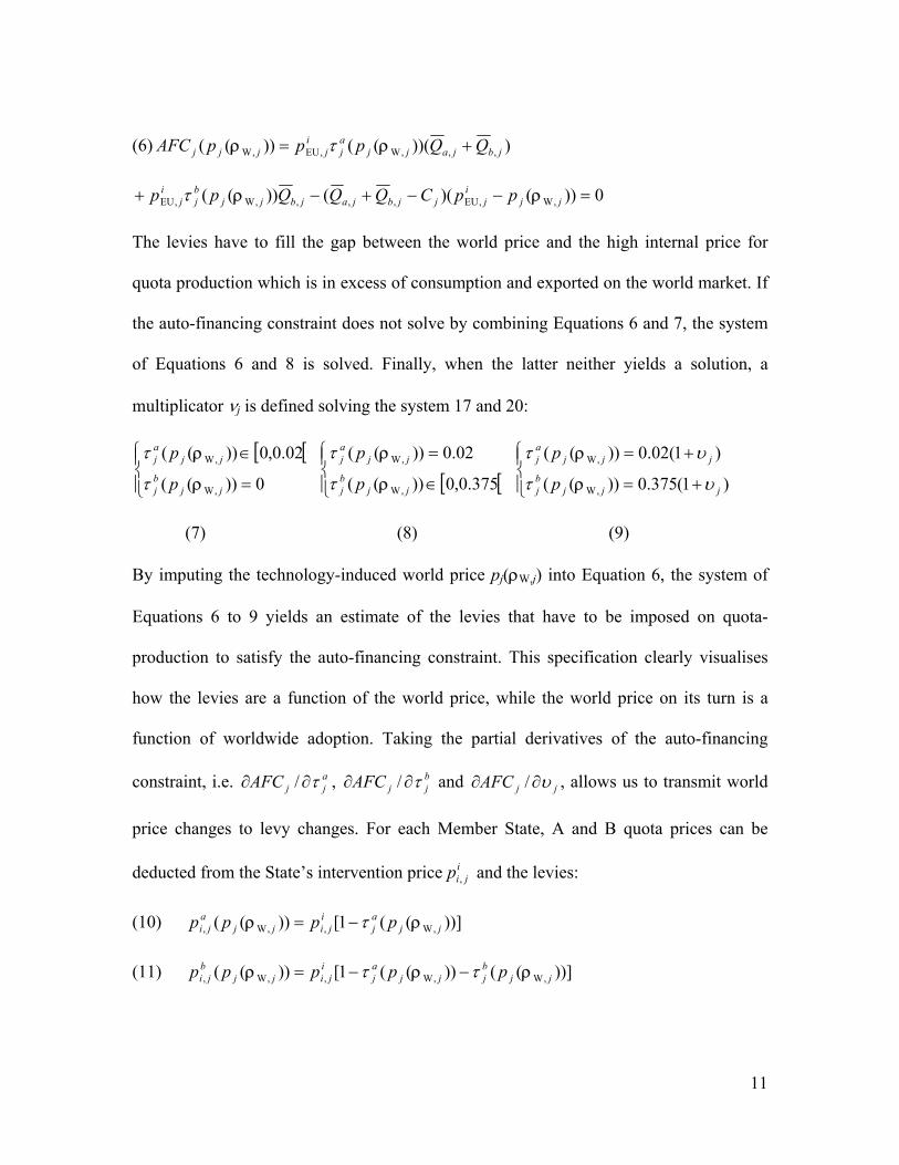
(6) )))((())(( ,,,W,EU,W jbjajjaj

ijjjj QQpppAFC += ρρ τ

0))()(())(( ,W,EU,,,,W,EU =−−+−+ jji

jjjbjajbjjbj

ij ppCQQQpp ρρτ

The levies have to fill the gap between the world price and the high internal price for

quota production which is in excess of consumption and exported on the world market. If

the auto-financing constraint does not solve by combining Equations 6 and 7, the system

of Equations 6 and 8 is solved. Finally, when the latter neither yields a solution, a

multiplicator νj is defined solving the system 17 and 20:

[ [

=

∈

0))((

02.0,0))((

,W

,W

jjbj

jjaj

p

p

ρ

ρ

τ

τ

[ [

∈

=

375.0,0))((

02.0))((

,W

,W

jjbj

jjaj

p

p

ρ

ρ

τ

τ

+=

+=

)1(375.0))((

)1(02.0))((

,W

,W

jjjbj

jjjaj

p

p

υτ

υτ

ρ

ρ

(7) (8) (9)

By imputing the technology-induced world price pj(ρW,j) into Equation 6, the system of

Equations 6 to 9 yields an estimate of the levies that have to be imposed on quota-

production to satisfy the auto-financing constraint. This specification clearly visualises

how the levies are a function of the world price, while the world price on its turn is a

function of worldwide adoption. Taking the partial derivatives of the auto-financing

constraint, i.e. ajjAFC τ∂∂ / , b

jjAFC τ∂∂ / and jjAFC υ∂∂ / , allows us to transmit world

price changes to levy changes. For each Member State, A and B quota prices can be

deducted from the State’s intervention price ijip , and the levies:

(10) ))]((1[))(( ,W,,W, jjaj

ijijj

aji pppp ρρ τ−=

(11) ))](())((1[))(( ,W,W,,W, jjbjjj

aj

ijijj

bji ppppp ρρρ ττ −−=

12

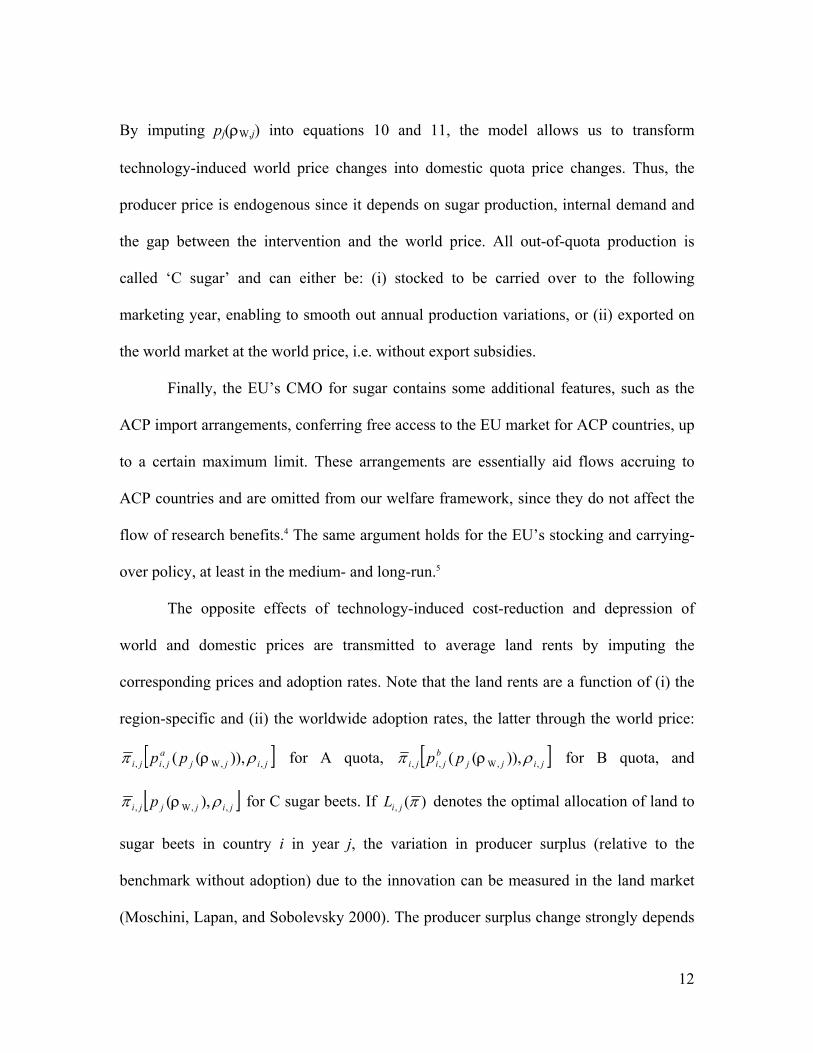
By imputing pj(ρW,j) into equations 10 and 11, the model allows us to transform

technology-induced world price changes into domestic quota price changes. Thus, the

producer price is endogenous since it depends on sugar production, internal demand and

the gap between the intervention and the world price. All out-of-quota production is

called ‘C sugar’ and can either be: (i) stocked to be carried over to the following

marketing year, enabling to smooth out annual production variations, or (ii) exported on

the world market at the world price, i.e. without export subsidies.

Finally, the EU’s CMO for sugar contains some additional features, such as the

ACP import arrangements, conferring free access to the EU market for ACP countries, up

to a certain maximum limit. These arrangements are essentially aid flows accruing to

ACP countries and are omitted from our welfare framework, since they do not affect the

flow of research benefits.4 The same argument holds for the EU’s stocking and carrying-

over policy, at least in the medium- and long-run.5

The opposite effects of technology-induced cost-reduction and depression of

world and domestic prices are transmitted to average land rents by imputing the

corresponding prices and adoption rates. Note that the land rents are a function of (i) the

region-specific and (ii) the worldwide adoption rates, the latter through the world price:

[ ]jijja

jiji pp ,,W,, )),(( ρπ ρ for A quota, [ ]jijjb

jiji pp ,,W,, )),(( ρπ ρ for B quota, and

[ ]jijjji p ,,W, ),( ρπ ρ for C sugar beets. If )(, πjiL denotes the optimal allocation of land to

sugar beets in country i in year j, the variation in producer surplus (relative to the

benchmark without adoption) due to the innovation can be measured in the land market

(Moschini, Lapan, and Sobolevsky 2000). The producer surplus change strongly depends

13

on the country’s competitiveness in sugar production. Therefore, we introduce a new

categorical parameter ϕi,j to denote the region’s production efficiency. Depending on the

value this parameter takes, the model automatically selects the appropriate formula for

the calculation of the welfare effects. Detailed information about the formulas can be

found in Dillen, Demont and Tollens (2007a). High-cost country i not fulfilling its A

quota gets ϕi,j = 0. Portugal and Greece are the only examples. Note that the benefit

resulting from the technology not only depends on the adoption within the region, but

also on worldwide adoption rates through the technology-induced world price

depreciation. A high-cost country, fulfilling its A but not its B quota is assigned φi,j = 1.

The farmers in these countries aim at fulfilling their A quota and in order to ensure this

objective they choose to accept a minimal precautionary overproduction, even in low-

yield years. For medium-cost countries fulfilling their A quota and a significant part of its

B quota, ϕi,j = 2. Exporting low-cost EU country responding to the world price at last get

ϕi,j = 4. According to different authors, different countries fulfil this criterion. A

combination of Frandsen et al (2003), a recalculation of Frandsen et al (2003) on data

an extended dataset (1996-2006), Poonyth (1998) and the success of the buy-out scheme

under the new CMO for sugar, gives Austria, Belgium, France, Germany, and the UK

complying with this criterion (Table 1, fulfilling three out of five criteria). Figure 1

illustrates graphically how the benefits are split up in (i) a within-quota (areas b – a), and

(ii) an out-of-quota part (areas d – c), earned on the world market. An exporting low-cost

EU region not responding to the world price (ϕi,j = 3) would normally not supply C-

sugar, since the rents of the latter are not sufficient to cover the production costs.

14

However, to ensure quota fulfilment farmers accept a risk premium (some out-of quota

production). Since quota fulfilment is the primary objective of these countries, we assume

that stock decisions and risk premiums are not affected by the new technology.

New Common Market Organisation for sugar (2006/2015)

On the first of July 2006 a new CMO for sugar was introduced. The key features

of the reform are (i) a progressive cut of the EU institutional price (the reference price)

up to 36% over four marketing years, (ii) direct compensatory payments of 64.2% of the

estimated revenue loss over three marketing years and (iii) a single quota arrangement for

the term 2006/07-2014/15. The goal of this reform is to reduce domestic EU sugar

production in order to comply with WTO, be prepared for the EBA and the commitment

of the EU to make agriculture more competitive. In order to facilitate this reduction in

production, a buy-out scheme is setup. Sugar producers giving up production due to the

lower prices can sell their quota to the EU for an in time decreasing amount (€730-€730-

€625-€520/ton). This should stimulate less competitive producers to reduce or abandon

production. If the reduction in production is insufficient in 2010, the EU can decide on a

linear quota cut for all European producers.

For the model this has several structural effects. A and B quota are replaced by one quota

with a price independent from the world market price, the reference price. The value of

parameter ϕi,j changes for all countries. Producers not filling their quota before

(ϕi,j=0,1or2), will sell their excess quota under the new institutional price and become

15

part of a group that fills their quota (ϕi,j=7). Producers filling their quota before (ϕi,j=3)

will also be part of this group although some selling of quota can occur due to the

reduced sugar prices. Having quota but not filling them is taxed by a restructuring amount

to be paid on each quota, a further incentive to sell excess quota. Countries which reacted

on world market prices before (ϕi,j=4) are affected the most. Due to a complained by the

WTO export of out of quota sugar (former C-sugar, 4 million ton) is very limited. Total

export from is limited by the WTO to 1.4million ton white sugar/year. Since this

allocation is first filled with excess quota sugar (as long as the budget is sufficient) and

can only be used for out of quota sugar in special cases, there aren’t any possibilities to

produce for the world market. However, under the new CMO for sugar, the possibility

exists to produce industrial sugar outside quota production. Competitive producers will

produce sugar for industrial use which means European industrial users will import less

sugar off the world market. This decrease in demand on the world market makes that the

EU still influences the world market to some extent.

The ROW cane industry is assumed to respond to the world price, but since no

technology-induced surplus is generated by the model6, the change in producer surplus

reflects the losses of cane growers due to eroding world prices:

(12) ( )

( )

∫=∆jijjji

jji

p

pjijijjji dLpPS

,,W,

,

),(

0),0(,,,W, )()),((ρπ

π

ππρρ

ρ

The ROW beet region can be considered ‘small’, i.e. facing an infinitely elastic export

demand function and not able to influence world prices significantly. Non-EU European

countries are part of this group. In addition, the US sugar sector is highly protected by a

16

tariff quota system, eliminating any link between domestic prices and supply and world

prices (Roberts and Wish-Wilson 1991). Therefore, neither supply shift nor negative

export demand shift are assumed for the ROW region, i.e. EDj(p,0) = EDj(p, ρROW,j) in

Figure 1. Instead of allocating more land, the ROW beet region responds to new

technologies by freeing up land allocated to sugar beet. This implies that innovation rents

for these regions can be calculated as:

(13) ( ) ( ) ( )[ ]0),0(),(),(

)),(( ,,,W,,,W

,,,W, jjijijjji

jijj

jijijjji pp

pyQ

pPS πρπρ

ρ −=∆ ρρ

ρ

The EU’s aggregate welfare increase is simply the sum of all production blocks’ producer

surplus changes:

(14) )),(()),(( ,,W

19

2,,EU,W,EU jijj

ijijjjj pPSpPS ρρρ ∑

=

∆=∆ ρ

In Figure 1, the aggregate benefit for the EU can be assessed by a pivotal shift of the

aggregate EU supply function. The exported surplus Qd is subsidised, since it receives the

guaranteed B quota price, while it is exported at the world price. Decline of the world

price from pj(0) to pj(ρW,j) raises subsidy costs up to Qd (pj(0) – pj(ρW,j)), represented by

the lower area a. These extra costs have to be borne by the producers via increased levies

on their quota production (Equations 6 to 9). In most cases, adapting only the B quota

levy is sufficient, visualised in Figure 1 through a decline of the B quota price. Hence, the

cost for producers equals ))](())0(([ ,W,, jjb

jijb

jib ppppQ ρ− , represented by the upper area

a, which is essentially the same as the lower area a. Thus, the total within-quota benefits

equal area b – a. To these rents, out-of-quota benefits have to be added, represented by

17

the difference between areas d and c. The EU’s change in consumer surplus can be

modelled as:

(15) ∫ ==∆)0),0((

)),((,EU,EU,W,

,EU

,EU,W,EU

0)()),((j

ij

jjji

j

pp

ppjjjjjEU dppDpCS

ρρ

ρρ

In our model however, the EU’s intervention price is fixed, so it is neither a function of

the world price, nor of the adoption rate within the EU:

(16) ijjjj

ij ppp ,EU,EU,W,EU )),(( =ρρ

This means that technology-induced welfare effects for consumers would only be

possible in the long term within the CMO for sugar if the EU endogenised world prices

and/or technology adoption rates in their intervention/reference price. In contrast, world

price changes are endogenous to producer prices through the auto-financing constraint.

The ROW aggregate innovation rents (area g – e in Figure 1) are simply the sum of cane

(i = 0) and beet (i = 1) producers’ surplus changes:

(17) ∑=

∆=∆1

0,,W,,ROW,W,ROW )),(()),((

ijijjjijjjj pPSpPS ρρρρ

The ROW consumers’ surplus change (area e + area f in Figure 1) equals:

(18) ∫=∆)0(

)(,ROW,ROW,W,ROW

,W

)()),((j

jj

p

pjjjjj dppDpCS

ρ

ρρ

Finally, to calculate the profit of the input suppliers, we need an estimate for all regions i

of the supply of land to the sugar beet industry in equilibrium: ]),([ ,,W, jijjji pL ρρ . Note

again the double dependence of land supply on local as well as global adoption rates, the

latter through the technology-induced world price depreciation. Again, we include the

18

possibility for some regions not responding to world prices, to respond to the new

technology by freeing up land allocated to sugar beet. In that case the yield-increasing

effect of the new technology negatively affects its own demand, due to the quota system.

The profit of the input suppliers can now be computed as:

(19) iijijji

jijijjjj wpLp δµρρ )),(()),(( ,,W

18

0,,,W,W ρρρ ∑

=

=Π

Total welfare increase is simply the sum of all welfare increases. Finally, by using a risk

adjusted rate of return of 10.5%, derived from the CAPM7, we can aggregate all year-

specific welfare changes and actualise them to the year 2006/07.

Data and model calibration

In our simulation model we assume hypothetically that both the EU’s beet sugar

industry, being a competitive player in the world market, and the ROW beet region

embraced the new technology since the marketing year 1996/97, and progressively

adopted it up to 2014/15. Our model is calibrated on the observed production data from

this period. Observed yields (yi,j), ‘incentive prices’ (see below), London n°5 world sugar

prices, quantities ( jiQ , ) and quota ( ajiQ , and b

jiQ , ) are taken from various sources

(European Commission 1999;F.O.Licht 2001;FAO 2006;F.O.Licht 2005;USDA 2006b).8

Data for the future come from the FAPRI model, extrapolations of historical trends

(yield/ha) and from decision 290/2007 from the EU. We assume only the efficient

producers (ϕi,j=8), produce industrial sugar and this up to an amount of 1.5 million ton

(SUBEL 2007) shared weighted on their quota. The other Member States are assumed to

19

just fill their quota. To calibrate the average rent function, we need an approximate

estimate of the observed land rent in all regions.9 Thelen (2004) compares per-hectare

profits among four beet producers (Poland, Ukraine, USA and Germany) and six cane

producers (Brazil, Australia, Thailand, South-Africa, India and USA). We use the

estimate of Germany for the EU-15 and calculate the area-weighted averages for the

ROW cane and beet regions. All cost and price data are first deflated and actualised to the

agricultural season 2006/07 using the GDP country deflators form the world development

indicators, and then converted to Euro using the exchange rate of 2006. Institutional

prices are deflated using both agricultural and financial exchange rates. Because HT

sugar beet is not yet adopted, we estimate the adoption parameters of a comparable

technology in the USA, i.e. HT Roundup Ready® soybeans(USDA 2006a)10. Therefore,

we first transform the logistic adoption curve (Griliches 1957): )1(,jba

ijiiieK ++=ρ

into its log-linear form:

(20) tbat

tii

ii

i,,

max, )()(

ln ρρρρρ

+=

−.

By assuming a ceiling of ρmax,US = 0.9, the estimated OLS parameters using linear

regression are aρ,US = 2.49, and bρ,US = 0.61. As a benchmark for HT sugar beet in the

EU, we assume a logistic adoption curve with the same constant of integration, aρ,US, and

adoption speed, bρ,US, as in the US. ρmax,i,j is calculated as in Dillen, Demont and Tollens

(2007b). We assume the innovating firm set their technology fee ( µ ) in 1996 upon

introduction of the technology and in 2004 with the introduction of 10 New Member

States. Distribution were created based on herbicide and application costs from Hermann

20

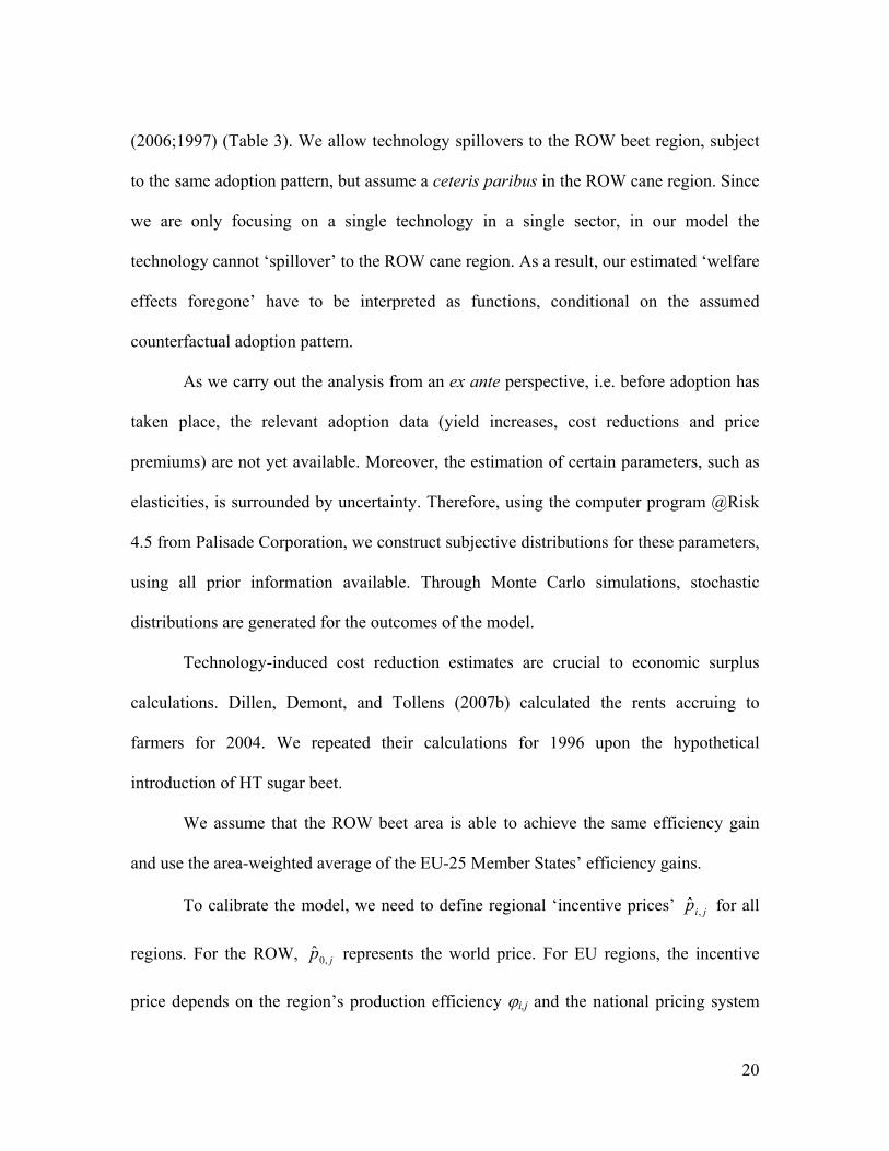
(2006;1997) (Table 3). We allow technology spillovers to the ROW beet region, subject

to the same adoption pattern, but assume a ceteris paribus in the ROW cane region. Since

we are only focusing on a single technology in a single sector, in our model the

technology cannot ‘spillover’ to the ROW cane region. As a result, our estimated ‘welfare

effects foregone’ have to be interpreted as functions, conditional on the assumed

counterfactual adoption pattern.

As we carry out the analysis from an ex ante perspective, i.e. before adoption has

taken place, the relevant adoption data (yield increases, cost reductions and price

premiums) are not yet available. Moreover, the estimation of certain parameters, such as

elasticities, is surrounded by uncertainty. Therefore, using the computer program @Risk

4.5 from Palisade Corporation, we construct subjective distributions for these parameters,

using all prior information available. Through Monte Carlo simulations, stochastic

distributions are generated for the outcomes of the model.

Technology-induced cost reduction estimates are crucial to economic surplus

calculations. Dillen, Demont, and Tollens (2007b) calculated the rents accruing to

farmers for 2004. We repeated their calculations for 1996 upon the hypothetical

introduction of HT sugar beet.

We assume that the ROW beet area is able to achieve the same efficiency gain

and use the area-weighted average of the EU-25 Member States’ efficiency gains.

To calibrate the model, we need to define regional ‘incentive prices’ jip ,ˆ for all

regions. For the ROW, jp ,0ˆ represents the world price. For EU regions, the incentive

price depends on the region’s production efficiency ϕi,j and the national pricing system

21

applied to pay beet growers and processors. The incentive prices for the former CMO for

sugar are modelled in a dynamic way and depend on the world price, which, on its turn,

depends on world-wide adoption rates. Incentive prices can be A sugar prices

))(( ,W, jja

ji pp ρ , B sugar prices ))(( ,W, jjb

ji pp ρ , a region-specific mixed price

[ ])()),(()),(( ,W,W,,W,, jjjjb

jijja

jim

ji pppppp ρρρ , or the world price pj(0)). For the new CMO

for sugar the incentive price for in quota sugar ( ojip , ) is fixed (although decreasing in

time) and the out of quota incentive price is the world price pj(0). The model is calibrated

on the pre-innovation equilibrium, i.e. we set ρW,j = 0.

In Table 2 we combine different sources to define the regions’ production

efficiencies, incentive prices and supply elasticities. Structural parameters such as supply

elasticities σ and demand elasticities ε are taken from the literature (see Table 2). To

calibrate θi,j, it is useful to relate this parameter to the more standard notion of elasticity

of land supply with respect to sugar prices. If we define ri,j as the farmer’s share (rent) of

unit revenue, the parameter θi,j can be calibrated as (Sobolevsky, Moschini, and Lapan

2005, p. 632):

(21)

==

jiji

iijiiji yp

r,,

,, ˆπ̂

ψψθ

Since our model features disaggregated area response (ψi) and yield response (ηi) to

prices (ψ = (∂L/∂p)(p/L) ≥ 0, η = (∂Y/∂p)(p/Y) ≥ 0 and ζ = ψ + η), we need to find

elasticities that correctly represent farmers’ behaviour and incentives in the global sugar

beet industry. In a quota system with fixed prices, annual within-quota price variation is

22

too small to obtain reliable estimates of supply response. While quota rents of world price

irresponsive regions are not significantly affected by supply response, world price

responsive regions significantly affect world prices and global welfare through

technological innovation. Therefore, for these regions in particular, i.e. Germany,

Belgium, France, Austria and the UK, precise estimates of supply response to world

prices are needed. Poonyth et al. (2000) report short- and long-run area elasticity

estimates for all EU-15 Member States, except Portugal and Greece. As Poonyth et al.

(2000) do not include any standard deviations for ψi, we construct symmetric triangular

distributions with the short-run estimate as minimum value, the long-run estimate as

maximum value and the medium-run, i.e. the average of both estimates, as most likely

value. For the export supply flexibilities σ1 and σ2 (Equation 5), we construct symmetric

triangular distributions, centred on the base value and ranging from zero to twice the base

value. Devadoss and Kropf (1996) report supply elasticities for all major sugar producers

in the world. For the ROW cane and ROW beet regions, we calculate a production-

weighted average supply elasticity of 0.269 and 0.207, respectively, and a consumption-

weighted average demand elasticity εROW of -0.034.11 For Greece and Portugal we use

Devadoss and Kropf’s (1996) supply elasticity estimate of 0.228 for A quota sugar. As

supply elasticities ζi already incorporate yield response to prices, we set ηi = 0 for these

regions. For EU-25 regions we use the yield response to prices from the ESIM-model12

(Banse, Grethe, and Nolte 2005), ηi = 0.08 surrounded by a triangular distribution

constructed analogously to the rest of the elasticities. The ESIM-model also supplies us

with supply elasticities for the New Member States.

23

Given the assumed, estimated and retrieved parameters, structural parameters,

such as Ai,j, Gi,j, and λi,j are calibrated so as to retrieve pre-innovation acreage, quantity,

yield and price data for each year j.

We allow technology spillovers to the ROW beet region, subject to the same

adoption pattern, but assume a ceteris paribus in the ROW cane region. Since we are only

focusing on a single technology in a single sector, in our model the technology cannot

‘spillover’ to the ROW cane region. As a result, our estimated ‘welfare effects foregone’

have to be interpreted as functions, conditional on the assumed counterfactual adoption

pattern.

Results

We conduct a Monte Carlo simulation of 6000 simulations to generate stochastic

distributions for our welfare estimates, using the @Risk software. Table 4 reports the

mean values. The downstream sector captures the largest share (61%) of the benefits.

This result is in line with the ex post impact studies on first generation GM crops which

show a distribution of 2/3 downstream, 1/3 upstream. 31% of the benefits is accruing to

the ROW if we assume that beet producers in these countries are able to achieve the same

efficiency enhancing effects trough the new technology, and are not able to export the

technology-induced export on the world market which would further erode the world

market price. Worldwide sugar beet growers gain €8.22 billion almost equally shared

between EU-25 producers (58%) and ROW producers (42%). The input suppliers (seed

24

industry and gene developers) extract €6.07 billion of the global welfare gain. If we do

not take into account any market effects, 58% of the benefits flow to the beet growers,

while 42% accrues to the input industry.

The depressing effect on world prices engendered by innovating world price

responsive regions causes ROW consumers to gain €8.64 billion, but this is largely offset

by the ROW cane growers’ loss of €7.25 billion. Since we assume that the technology

spillovers to the ROW beet sector do not depress the world price, the EU is not affected.

Instead, the world price responsive EU region is able to erode its own profitability

through technological innovation, an ambiguity called ‘immiserising growth’ (Bhagwati

1958), but our results show that the CMO for sugar largely protects domestic producers

against this perverse side effect of innovation. The model suggests a world price decrease

of 1.6% is expected to occur over a period of 19 years, a annual decrease of 1.3%.

Compared with other studies, reporting annual price declines of 0.64% due to the

adoption of Bt cotton in the USA (Falck-Zepeda, Traxler, and Nelson 2000) and 0.88%

(Moschini, Lapan, and Sobolevsky 2000) and 0.97% (Qaim and Traxler 2005) due to the

adoption of Roundup Ready® soybeans in the USA and South America, our estimate is

relatively big but this is due to the bigger time span of our study.

Since EU institutional prices are exogenously fixed13, no important price declines

are possible. As a result, the benefits essentially flow to farmers without affecting EU

processors and consumers. However, if weed control based on transgenic HT technology

increases the sugar beet’s sucrose content (Kniss et al. 2004), processors will gain as the

processing costs are approximately the same per ton of beets regardless of sugar content

25

(DeVuyst and Wachenheim 2005). Moreover, if the EU government endogenised public

and private agricultural research expenditures (see e.g. Swinnen and De Gorter 1998) in

the CMO for sugar, benefits would be shared among farmers and consumers. The global

welfare gain, finally, amounts to €15.68 billion after 19 years of adoption.

As we assume no supply response for the majority of beet producers, the

enhanced yields of the new technology engender important land contractions in the beet

industry. Table 4 presents the average land supply response (LSR). Our model predicts

that due to the adoption of HT sugar beet, the EU-25 beet area will shrink 1.2% on

average. World price irresponsive Member States’ areas are expected to decline between

1.99% and 4.29%, whereas world price responsive regions are expected to allocate more

land to sugar beet, i.e. between 0.18% and 0.63%, in response to increased profits. The

ROW beet region will remove 2.75% of sugar beet area from cultivation, while the ROW

cane area shrinks with 0.37%. On the global scale, the sugar industry is expected to

contract its area allocation to sugar beet and cane with an average of 0.70%.

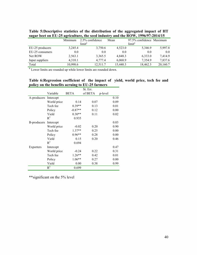
In Table 5, we present some descriptive statistics of the generated welfare

estimates. Given the assumed subjective distributions, reflecting the uncertainty in the

data, EU-25 producer surplus ranges from € 3,750 billion to €5,347 billion in 95% of the

cases. Total welfare increase is lest robust, ranging with the same probability from €12.5

billion to €18.5 billion.

The reform of the CMO for sugar in 2006 will affect the benefits accruing to

farmers. The effect is studied by a multiple regression on the production weighted

average for each group of sugar producers, A-producers (ϕi,j=0,1), B-producers14

26

(ϕi,j=2,3), exporters (ϕi,j=4). The variables used are yield, world price, technology fee

(which depends on the heterogeneity among farmers) and a dummy variable for the

change in policy. The results in Table 6 show A- producers will be negatively affected

during the restructuring period and even more there after. This because the reference

price for sugar (PR) is between A en B quota prices, i.e. pb<PR<pa. B-producers gain from

the new policy. Most of this gain in generated in the restructuring period during which

the reference price is much higher than the B-sugar price. After restructuring the new

CMO affects their innovation rents less. C-producers also gain significantly from the new

technology due to the less disturbing effect of EU sugar exports on the world market. It

seems the regime is tailored towards efficient producers and will probably lead towards

the crowding out of inefficient A-producers. This is exactly what the purpose of this

reform was. Besides these expected effects, some counterintuitive results come up. The

technology fee has a significant positive effect for each group of producers. This is the

case because tech fee is based on herbicide expenditures which decreased through time

through better management and products. In further analyses it seems the herbicide

expenditures could be a better variable to regress. The insignificant effect of world prices

is not expected either. The independence of the producer welfare of the world market

allows some more advanced stochastic testing in the next part of our research.

27

Conclusion

We developed a model shaped to the European sugar sector to assess the size and

distribution of the benefits of genetically modified sugar beet adoption in the EU-25 and

the ROW. The potential size of benefits is large with a €15 billion worldwide. These

benefits are not created at the moment due to the risk acceptance of consumers

worldwide. The framework suggests 39% of the created welfare accrues to the input

industry while 61% of the created welfare goes to the downstream sector (farmers and

consumers). This is in line with the rule of thumb of 1/3 versus 2/3 as found in ex post

impact assessments. The share of benefits going to farmers and consumers is divided

between ROW and EU-25 (31%-30%). Cane growers in the world lose due the

depressing effect of the innovation on world sugar prices. Consumers outside the EU

profit from this price reduction while EU consumers do not profit from the innovation in

the short run due to fixed prices in the CMO for sugar. The technology induced land

contraction in the EU is estimated -1.2%. Inefficient producers lose significantly more (<-

3%) while efficient, exporting countries can even expand there allocated area slightly.

The reform of the CMO for sugar in 2006 had a significant effect on the farmer rents due

to reduced sugar prices. The efficient producers gain more under the new CMO while the

inefficient losers seem to lose rents. The reform is tailored to efficient producers an

promotes innovations in the sugar sector. Crowding out of inefficient A producers could

take place, as is one of the incentives of the reform.

28

1 In the literature, the monopoly rents of the innovators are calculated as gross technology revenues. No

research, marketing or administration costs are deducted, because such data are not easily available. If these

costs were deducted, the general rule of thumb could rather become ‘one quarter upstream versus three

quarters downstream’. For an example of a study incorporating such data, see Phillips (2003).

2 We are grateful to Brent Borrell (CIE, Canberra) for pointing this out.

3 According to Gohin and Bureau (2006), various world sugar market liberalisation studies produce

inconsistent results because of the incorrect modelling of EU supply response. Therefore, using an

aggregate function that summarizes heterogeneous individual behaviours is one way to deal with the

problem.

4 Ivan Roberts correctly points out that this is so as long as the aid is maintained. But if it were to be

discontinued, it would raise world prices, influencing C-sugar and B-sugar returns.

5 In the short run, producers could stock surpluses generated by the innovation, but this ‘hold-up’ of R&D

benefits is temporal as the stocks are limited to 20% of the A quota (European Commission 1996).

6 Our ceteris paribus assumption implies that transgenic technology is only adopted in the beet sector.

7 We assume that the conditions for the CAPM (capital asset pricing model) do hold. The risk adjusted rate

of return is the sum of the risk premium and the risk-free rate of return (ROR). We assume a risk premium

of 8%, based on the New York Stock Exchange (see Dixit and Pindyck 1994) and added a 2.5% risk-free

ROR from the European Central Bank in 1995, getting a 10.5% risk adjusted ROR.

8 We assume complete market clearance, i.e. stock decisions are not affected by the new technology.

9 After an extensive sensitivity analysis it appears that this is just an inconsequential scaling parameter,

which is in line with the observations of Moschini, Lapan, and Sobolevsky (2000, p. 46).

10 We believe that the US case of HT Roundup Ready® soybeans is comparable with the EU case of HT

sugar beet, because of (i) the common embedded technology of herbicide tolerance, (ii) the ubiquitous

importance of each crop on both continents, and (iii) the importance of exports of the refined products.

29

11 Supply elasticities of sugar cane are inelastic in the short run since several annual crops can be harvested

from one planting of cane whereas beet is an annual crop.

12 The elasticities from the ESIM-model are behavioral elasicities while the others are econometric

elasticities.

13 In the new CMO, prices can be assumed to be fixed due to the intervention mechanism in the policy in

case of long term price declines.

14 The Netherlands and Ireland are excluded from the analysis due to there mixed price system. Ireland

stopped producing under the new CMO. The regression on the Netherlands showed policy has a significant

positive effect on the farmers rent (1.8) bigger than for other B-producers. The reason can be found in the

lower price they were paid due to the mixed price before the reform.

30

References

Alston,J.M., G.W.Norton, and P.G.Pardey Science under scarcity: principles and

practice of agricultural research evaluation and priority setting. Ithaca, NY:

Cornell University Press, 1995.

Banse,M., H.Grethe, and S.Nolte. Documentation of the ESIM model structure, base data

and parameters. 2005. Göttingen and Berlin, University of Göttingen and

Humboldt University.

Bhagwati,J.N. "Immiserizing growth: A geometrical note." Review of Economic Studies

25(1958): 201-5.

Brookes,G. "The farm-level impact of herbicide-tolerant soybeans in Romania."

AgBioForum 8(2005): 235-41.

Combette,P., E.Giraud-Heraud, and V.Réquillart "La politique sucrière européenne après

les accords du GATT: Une analyse de quelques scénarios d'évolution." Economie

et Prévision 127(1997): 1-13.

Confédération des Betteraviers Belges. 2002.

Demont,M. "Economic impact of agricultural biotechnology in the European Union."

Doctoral Dissertation, Katholieke Universiteit Leuven, 2006a.

31

-----. Economic impact of agricultural biotechnology in the European Union: Transgenic

sugar beet and maize. 713, 1-134. 2006b. Leuven, Katholieke Universiteit

Leuven. Dissertationes de Agricultura.

Demont,M. et al. "GM crops in Europe: How much value and for whom?" EuroChoices

Forthcoming(2007).

Demont,M. and E.Tollens "Ex ante welfare effects of agricultural biotechnology in the

European Union: The case of transgenic herbicide tolerant sugarbeet." The

regulation of agricultural biotechnology. Robert E. Evenson and Vittorio

Santaniello, eds., pp. 239-55. Wallingford, UK: CAB International, 2004a.

----- "First impact of biotechnology in the EU: Bt maize adoption in Spain." Annals of

Applied Biology 145(2004b): 197-207.

Demont,M., J.Wesseler, and E.Tollens "Biodiversity versus transgenic sugar beet: The

one euro question." European Review of Agricultural Economics 31(2004): 1-18.

Devadoss,S. and J.Kropf "Impacts of trade liberalizations under the Uruguay Round on

the world sugar market." Agricultural Economics 15(November 1996): 83-96.

DeVuyst,C.S. and C.J.Wachenheim "American Crystal Sugar: Genetically enhanced

sugarbeets?" Review of Agricultural Economics 27(2005): 105-16.

32

Dillen,K., M.Demont, and E.Tollens. Global welfare effects of genetically modified sugar

beet under changing EU sugar trade policies. 100, 1. 2007a. Leuven, Katholieke

Universiteit Leuven. Working Paper.

-----. Modelling heterogeneity to estimate the ex ante value of biotechnology innovations.

99, 1. 2007b. Leuven, Katholieke Universiteit Leuven. Working Paper.

Dixit,A. and R.S.Pindyck Investment under uncertainty. Princeton: Princeton University

Press, 1994.

European Commission. Sugar. 1-25. 1996. Office for Official Publications of the

European Communities Luxembourg. CAP Working Notes 1996/97.

----- The agricultural situation in the European Union: 1998 report. Luxembourg: Office

for Official Publications of the European Communities, 1999.

F.O.Licht World sugar statistics 2002. Kent: F.O.Licht, 2001.

----- World sugar yearbook 2006. Kent: F.O.Licht, 2005.

Falck-Zepeda,J.B., G.Traxler, and R.G.Nelson "Surplus distribution from the introduction

of a biotechnology innovation." Am J Agricultural Economics 82(May 2000):

360-9.

FAO FAOSTAT agriculture data. Rome: FAO, 2006.

33

Flannery,M.-L. et al. "An economic cost-benefit analysis of GM crop cultivation: An

Irish case study." AgBioForum 7(2004): 149-57.

Frandsen,S.E. et al. "Reform of EU sugar policy: Price cuts versus quota reductions."

European Review of Agricultural Economics 30(2003): 1-26.

Frisvold,G.B., J.Sullivan, and A.Raneses "Genetic improvements in major US crops: The

size and distribution of benefits." Agricultural Economics 28(2003): 109-19.

Gohin,A. and J.-C.Bureau "Modelling the EU sugar supply to assess sectoral policy

reforms." European Review of Agricultural Economics 33(2006): 223-47.

Griliches,Z. "Hybrid corn: An exploration in the economics of technological change."

Econometrica 25(October 1957): 501-22.

Hermann O. "Survey on pests and diseases in sugar beet growing and the cost of plant

protection products in Europe." CIBE congress 2006. Cracow: 2006.

Hermann,O. "Enquête sur le coût de la lutte phytosanitaire dans la culture de la betterave

sucrière en Europe." IIRB 60th Congress Proceedings., pp. 469-75. Brussels:

IIRB, 1997.

James,C. Global Status of Commercialized Biotech/GM Crops: 2006. 35. 2006. Ithaca,

NY, ISAAA. ISAAA Brief.

Kniss,A.R. et al. "Economic evaluation of glyphosate-resistant and conventional sugar

beet." Weed Technology 18(2004): 388-96.

34

Moschini,G. and H.E.Lapan "Intellectual property rights and the welfare effects of

agricultural R&D." Am J Agricultural Economics 79(1997): 1229-42.

Moschini,G., H.E.Lapan, and A.Sobolevsky "Roundup Ready soybeans and welfare

effects in the soybean complex." Agribusiness 16(2000): 33-55.

Nielsen,C.P. and K.Anderson "Global market effects of alternative European responses to

genetically modified organisms." Weltwertschaftliches Archiv 137(2001): 320-46.

Phillips,P.W.B. "The economic impact of herbicide tolerant canola in Canada." The

economic and environmental impacts of agbiotech: A global perspective.

Nicholas G. Kalaitzandonakes, ed., pp. 119-39. New York: Kluwer

Academic/Plenum Publishers, 2003.

Poonyth,D. "A structural econometric model of European Union sugar industry and the

potential implications of the GATT WTO." Ph.D. Dissertation, Faculty of the

Graduate School, University of Missouri-Columbia, 1998.

Poonyth,D. et al. "Impacts of WTO restrictions on subsidized EU sugar exports."

Agricultural Economics 22(April 2000): 233-45.

Qaim,M. and G.Traxler "Roundup Ready soybeans in Argentina: farm level,

environmental, and welfare effects." Agricultural Economics 32(2005): 73-86.

Roberts,I. and P.Wish-Wilson. Domestic and world market effects of EC sugar policies.

91.1, 1-66. 1991. Canberra, ABARE. ABARE Discussion Paper.

35

Sobolevsky,A., G.Moschini, and H.E.Lapan "Genetically modified crop innovations and

product differentiation: Trade and welfare effects in the soybean complex." Am J

Agricultural Economics 87(2005): 621-44.

SUBEL. 2007. Personal Communication

Swinnen,J.F.M. and H.De Gorter "Endogenous commodity policies and the social

benefits from public research expenditures." Am J Agricultural Economics

80(1998): 107-15.

Thelen,M. "What are the main forces operating on the world market?" Courier 1(2004).

USDA. Adoption of Genetically Engineered Crops in the U.S. United States Department

of Agriculture . 2006a.

----- "EU25 sugar semi anual." Gain report. 2006b.

van Meijl,H. and F.van Tongeren "International diffusion of gains from biotechnology

and the European Union's Common Agricultural Policy." Agricultural Economics

31(December 2004): 307-16

36

Table 1: Competitiveness of sugar beet production for each Member State Frandsen,2003 Frandsen,

revisiteda Poonyth,1998 Gohin,2006 Buy-out in first 2

year Belgium + Luxembourg Include Include No Danmark Include No Germany Include Include Include Include No Greece Yes Spain Yes France Include Include Include No Ireland wrongb Yes Italy Yes the Netherlands Include No Austria Include Include No Portugal Yes Finland Yes Sweden Include Yes United Kingdom Include Include wrongb Include No Czech republic Include Yes Hungary Include Yes Poland Include No a The criteria used by Frandsen on an extended data set (1996-2006) b The mixed price used is wrong (Frandsen et al. 2003;Gohin and Bureau 2006;Poonyth 1998)

Table 2: Regional specification of incentive prices and elasticities Region ϕi

Incentive price Area elasticity Yield elasticity

former new former new ROW cane 6 6 world price world price 0.290 0 ROW beet 5 5 world price world price 0.202 0 Belgium 4 8 world price (C) world price (ind) 0.055 0.08 Denmark 3 7 B sugar price instit. price 0.034 0.08 Germany 4 8 world price (C) world price (ind) 0.074 0.08 Greece 0 7 A sugar price instit. price 0.228 0 Spain 3 7 B sugar price instit. price 0.226 0.08 France 4 8 world price (C) world price (ind) 0.172 0.08 Ireland 2 7 mixed price (A, B and C sugar) instit. price 0.034 0.08 Italy 1 7 A sugar price instit. price 0.712 0.08

Netherlands 2 7 mixed price (A, B and a fixed quantity of C sugar)

instit. price 0.041 0.08

Austria 4 8 world price (C) world price (ind) 0.154 0.08 Portugal 0 7 A sugar price instit. price 0.228 0 Finland 1 7 A sugar price instit. price 0.064 0.08 Sweden 2 7 B sugar price instit. price 0.030 0.08 United Kingdom 4 8 world price (C) world price (ind) 0.176 0.08

Czech Republic 4 7 world price (C) instit. price 0.569 0.08 Hungary 3 7 B sugar price instit. price 0.5686 0.08 Poland 3 7 B sugar price instit. price 0.5667 0.08 Sources: Devadoss and Kropf (1996), Poonyth et al. (2000), Confédération des Betteraviers Belges (2002) and Frandsen et al. (2003), Banse, Grethe, and Nolte (2005)

37

Table 3:Heterogeneity among farmers, technology fee and maximal adoption following Dillen, Demont and Tollens (2007) Loglogistic(0, δγ , ) µ ρmax,i,j γ δ

1996 2004 1996 2004 1996 2004 1996 2004Belgium 163.74 206.59 8.3785 4.2293 98 88 89% 91%Denmark 165.51 165.51 4.3522 4.3522 98 88 88% 92%Germany 202.04 160.33 4.9939 3.9367 98 88 90% 69%Greece 223.55 121.06 9.067 10.519 98 88 99% 63%Spain 265.37 222.94 5.5183 6.0868 98 88 100% 100%France 124.76 135.78 4.7872 9.7149 98 88 43% 89%Ireland 196.52 84.422 9.9645 9.68 98 88 93% 1%Italy 184.83 145.32 5.7751 6.3659 98 88 74% 53%The Netherlands 123.5 164.32 3.2706 13.483 98 88 69% 100%Austria 229.12 260.8 4.729 5.4323 98 88 87% 96%Portugal 265.37 265.37 5.5183 5.5183 98 88 99% 100%Finland 266.13 200.67 6.514 10.044 98 88 99% 100%Sweden 139 148.56 3.4986 4.2881 98 88 47% 60%United Kingdom 124.05 124.05 5.9299 5.9299 98 88 66% 73%Czech Republic 180.12 9.9884 88 92%Hungary 132.28 2.7296 88 46%Poland 184.91 6.3962 88 87%

38

Table 4:Price and welfare effects (in million euros) of the adoption of herbicide tolerant sugar beet in the world Year Benchmark 1996/97 1997/98 1998/99 1999/00 2000/01 2001/02 2002/03 2003/04 2004/05 2005/06 1996/97

Price effects World sugar price (%) 100% 99.65% 99.59% 99.35% 99.09% 98.92% 98.73% 98.65% 98.49% 98.58% 98.66%A sugar price (%) 100% 99.99% 99.99% 99.99% 99.99% 99.97% 99.98% 99.97% 99.98% 99.99% 99.98%B sugar price (%) 100% 99.77% 99.77% 99.73% 99.70% 99.17% 99.48% 99.16% 99.26% 99.56% 99.37% Welfare effects

Belgium 0.00 2.46 3.61 4.13 5.70 6.72 8.67 8.67 9.02 15.21 18.53Denmark 0.00 1.90 3.23 4.59 6.28 7.75 9.56 9.91 11.04 12.61 12.23Germany 0.00 12.70 18.53 24.46 31.12 39.79 48.13 48.17 49.08 44.21 53.55Greece 0.00 1.82 3.17 3.44 5.47 7.84 8.87 9.51 8.33 5.38 5.68Spain 0.00 9.10 15.47 22.04 30.27 38.07 44.49 44.88 50.76 45.90 44.06France 0.00 5.10 7.40 9.71 11.74 11.50 19.09 15.78 16.84 44.74 61.10Ireland 0.00 1.32 2.09 3.20 4.45 5.08 5.98 6.45 7.13 0.21 0.35Italy 0.00 5.67 9.21 13.64 18.61 22.74 27.09 28.66 34.37 21.91 21.75The Netherlands 0.00 3.71 6.60 10.50 13.88 15.83 20.00 20.27 22.47 34.09 33.65Austria 0.00 1.42 2.09 2.74 3.39 3.93 5.34 5.24 5.15 8.22 10.81Portugal 0.00 0.03 0.83 1.17 1.75 1.90 2.54 2.36 2.96 3.00 2.88Finland 0.00 1.02 1.48 2.57 3.24 4.11 4.83 5.13 5.78 4.94 4.98Sweden 0.00 0.64 1.09 1.58 2.32 2.93 3.45 3.97 4.19 4.88 5.32United Kingdom 0.00 2.62 3.97 4.93 6.03 6.50 9.51 8.56 8.98 13.25 16.42Czech Republic 0.00 0.00 0.00 0.00 0.00 0.00 0.00 0.00 0.00 15.44 14.85Hungary 0.00 0.00 0.00 0.00 0.00 0.00 0.00 0.00 0.00 9.12 8.56Poland 0.00 0.00 0.00 0.00 0.00 0.00 0.00 0.00 0.00 58.17 56.21EU-15 producers 0.00 49.51 78.77 108.69 144.25 174.68 217.53 217.54 236.09 341.29 370.93EU-15 consumers 0.00 0.00 0.00 0.00 0.00 0.00 0.00 0.00 0.00 0.00 0.00ROW cane 0.00 -116.46 -115.22 -148.77 -164.49 -238.67 -289.76 -300.04 -296.12 -310.02 -420.16ROW beet 0.00 39.56 67.42 89.95 115.36 154.36 161.54 187.03 181.99 175.09 207.94Net ROW producers 0.00 -76.90 -47.80 -58.83 -49.12 -84.31 -128.22 -113.00 -114.14 -134.93 -212.22ROW consumers 0.00 148.80 147.01 184.16 202.99 295.45 341.47 335.27 349.94 373.88 491.50Net ROW 0.00 71.90 99.21 125.33 153.86 211.14 213.25 222.27 235.80 238.95 279.28Input suppliers 0.00 75.33 113.68 169.04 233.93 277.06 307.68 352.17 363.58 359.78 355.16Total 0.00 196.75 291.66 403.06 532.05 662.89 738.46 791.98 835.48 940.02 1005.36 Welfare distribution

EU-15 producers (%) . 25% 27% 27% 27% 26% 30% 28% 28% 36% 37%EU-15 consumers (%) . 0% 0% 0% 0% 0% 0% 0% 0% 0% 0%Net ROW (%) . 36% 34% 31% 29% 32% 29% 28% 28% 25% 28%Input suppliers (%) . 38% 39% 42% 44% 42% 42% 45% 44% 38% 35%

Total (%) . 100% 100% 100% 100% 100% 100% 100% 100% 100% 100%

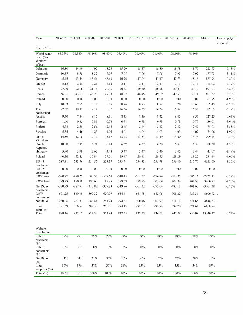
39

Year 2006/07 2007/08 2008/09 2009/10 2010/11 2011/2012 2012/2013 2013/2014 2014/2015 AGGR Land supply response Price effects

World sugar price (%)

98.33% 98.36% 98.40% 98.40% 98.40% 98.40% 98.40% 98.40% 98.40%

Welfare effects

Belgium 16.50 14.30 14.92 15.26 15.29 15.37 15.50 15.58 15.70 222.73 0.18%Denmark 10.87 8.75 8.32 7.97 7.97 7.96 7.95 7.93 7.92 177.93 -3.11%Germany 45.45 43.54 45.56 46.63 46.76 47.04 47.47 47.73 48.15 887.94 0.20%Greece 5.12 2.35 2.21 2.10 2.11 2.11 2.11 2.11 2.11 115.02 -2.77%Spain 27.00 22.18 21.18 20.35 20.33 20.30 20.26 20.23 20.19 691.01 -3.26%France 56.81 43.62 46.29 47.78 48.02 48.45 49.09 49.51 50.14 603.32 0.29%Ireland 0.00 0.00 0.00 0.00 0.00 0.00 0.00 0.00 0.00 63.75 -1.99%Italy 10.83 9.69 9.17 8.75 8.74 8.73 8.72 8.70 8.69 389.45 -2.23%The Netherlands

22.57 18.07 17.14 16.37 16.36 16.35 16.34 16.32 16.30 389.05 -3.17%

Austria 9.40 7.84 8.15 8.31 8.33 8.36 8.42 8.45 8.51 127.25 0.63%Portugal 1.60 0.85 0.81 0.78 0.78 0.78 0.78 0.78 0.77 36.01 -3.64%Finland 4.78 2.68 2.56 2.46 2.45 2.44 2.43 2.42 2.40 78.91 -3.58%Sweden 5.35 4.46 4.23 4.05 4.04 4.04 4.03 4.03 4.02 74.06 -1.99%United Kingdom

14.59 12.10 12.79 13.17 13.22 13.33 13.49 13.60 13.75 209.75 0.30%

Czech Republic

10.68 7.09 6.71 6.40 6.39 6.39 6.38 6.37 6.37 80.30 -4.29%

Hungary 5.90 3.79 3.62 3.48 3.48 3.47 3.46 3.45 3.44 45.07 -2.19%Poland 40.36 32.45 30.84 29.51 29.47 29.41 29.35 29.29 29.23 331.44 -4.06%EU-15 producers

287.81 233.76 234.52 233.37 233.74 234.53 235.78 236.49 237.70 4523.00 -1.20%

EU-15 consumers

0.00 0.00 0.00 0.00 0.00 0.00 0.00 0.00 0.00 0.00 .

ROW cane -520.77 -478.29 -508.50 -537.68 -548.45 -561.27 -576.74 -589.95 -606.16 -7222.11 -0.37%ROW beet 199.78 190.78 197.62 199.85 198.69 199.95 201.69 202.84 204.53 3460.72 -2.75%Net ROW producers

-320.99 -287.51 -310.88 -337.83 -349.76 -361.32 -375.04 -387.11 -401.63 -3761.38 -0.70%

ROW consumers

601.25 569.38 597.32 629.07 644.44 661.78 682.95 701.22 723.31 8609.72 .

Net ROW 280.26 281.87 286.44 291.24 294.67 300.46 307.91 314.11 321.68 4848.33 . Input suppliers

321.29 306.54 302.39 298.31 294.13 293.57 292.94 292.28 291.61 6068.94 .

Total 889.36 822.17 823.34 822.93 822.55 828.55 836.63 842.88 850.99 15440.27 -0.73% Welfare distribution

EU-15 producers (%)

32% 29% 29% 28% 29% 28% 28% 28% 28% 29%

EU-15 consumers (%)

0% 0% 0% 0% 0% 0% 0% 0% 0% 0%

Net ROW (%)

31% 34% 35% 35% 36% 36% 37% 37% 38% 31%

Input suppliers (%)

36% 37% 37% 36% 36% 35% 35% 35% 34% 39%

Total (%) 100% 100% 100% 100% 100% 100% 100% 100% 100% 100%

40

Table 5:Descriptive statistics of the distribution of the aggregated impact of HT sugar beet on EU-25 agriculture, the seed industry and the ROW, 1996/97-2014/15 Minimum 2.5% confidence

limita Mean 97.5% confidence

limita Maximum

EU-25 producers 3,245.4 3,750.6 4,523.0 5,346.9 5,997.8EU-25 consumers 0.0 0.0 0.0 0.0 0.0Net ROW 2,563.1 3,365.5 4,848.3 6,333.0 7,414.9Input suppliers 4,310.1 4,777.4 6,068.9 7,354.9 7,837.6Total 10,998.6 12,511.7 15,440.3 18,462.3 20,160.7a Lower limits are rounded up while lower limits are rounded down.

Table 6:Regression coefficient of the impact of yield, world price, tech fee and policy on the benefits acruing to EU-25 farmers St. Err. Variable BETA of BETA p-level A-producers Intercept 0.10 World price 0.14 0.07 0.09 Tech fee 0.39** 0.13 0.01 Policy -0.87** 0.12 0.00 Yield 0.30** 0.11 0.02 R2 0.935 B-producers Intercept 0.03 World price -0.02 0.20 0.90 Tech fee 1.37** 0.25 0.00 Policy 0.96** 0.28 0.00 Yield 0.15 0.20 0.46 R2 0.694 Exporters Intercept 0.47 World price -0.24 0.22 0.31 Tech fee 1.26** 0.42 0.01 Policy 1.06** 0.27 0.00 Yield 0.00 0.38 0.99 R2 0.699 **significant on the 5% level

41

Figure 1: Distribution of R&D benefits in the EU’s sugar sector with technology spillovers to the rest of the world (ROW)

pp

p

qq

q

QEU,j(p,0)

(a) E

U qu

antit

y(b

) Tra

ded

quan

tity

(c) R

OW

qua

ntity

p j(0)

Q a

D EU ,j(p)

C

dc

b

ef

g

a

∆PS EU

,j=

b –

a +

d –c

≥0

∆CS EU

,j=

0

∆PS EU

,j=

b –a

+ d

–c ≥

0

∆CS EU

,j=

0

∆PS RO

W,j

= g

–e ≤

0

∆CS RO

W,j

= e +

f >

0

∆PS RO

W,j

= g

–e ≤

0

∆CS RO

W,j

= e +

f >

0

Q b

Q c,0

Q c,1

Q c,0

Q c,1

Q e,0

Q e,1

Q d=

Q a+

Q b–C

a

QEU,j(p,ρEU,j)

ESj(p

,0)ES

j(p,ρ

EU,j)

EDj(p

,0)

EDj(p

,ρRO

W,j)

Q ROW

,j(p,0

)Q RO

W,j(p

,ρRO

W,j)

D ROW

,j(p)

p j(ρEU

,j)p j(ρ

W,j)

pa i,j(p

j(ρW

,j))

pb i,j(p

j(ρW

,j))

pi EU,j

pb i,j(p

j(0))