global warming -...
TRANSCRIPT

GLOBAL WARMING and AGRICULTURE
Impact Estimates by Country

This page intentionally left blank
Departemen Pendidikan Nasional
Universitas Tanjungpura Jl. Jenderal Ahmad Yani ‐
Telp/Faks 0561‐739630; 739637; Homepage: Pontianak – Kalimantan Barat – 78124
http://www.untan.ac.id
Drs. Erdi, M.Si Tenaga Pengajar
Kampus: FISIP, Universitas Tanjungpura Jl. Jenderal Ahmad Yani – Pontianak Telp.+62-561-740188; Faks.+62-561-571752; Email: [email protected]
Rumah: PERUMNAS IV TANJUNGHULU Jl. Sungai Sambas Barat 8, No.196, PTK HP +6281522535893 (Mentari) dan +6285234288831 (AS)
William R. Cline
C E N T E R F O R G LO B A L D E V E LO P M E N TP E T E R S O N I N S T I T U T E F O R I N T E R N A T I O N A L E C O N O M I C S
Wa s h i n g t o n , D CJ u l y 2 0 0 7
GLOBAL WARMING and AGRICULTURE
Impact Estimates by Country
William R. Cline is a senior fellow jointlyat the Center for Global Development(since 2002) and the Peterson Institute forInternational Economics (since 1981).During 1996–2001, he was deputy manag-ing director and chief economist at theInstitute of International Finance. He was asenior fellow at the Brookings Institution(1973–81); deputy director of developmentand trade research, office of the assistantsecretary for international affairs, USTreasury Department (1971–73); FordFoundation visiting professor in Brazil(1970–71); and lecturer and assistant pro-fessor of economics at Princeton University(1967–70). He is the author of 22 books,including The United States as a DebtorNation (2005), Trade Policy and Global Poverty(2004), Trade and Income Distribution (1997),International Debt Reexamined (1995), andThe Economics of Global Warming (1992),which was selected by Choice for its 1993“Outstanding Academic Books” list andwas the winner of the “Harold andMargaret Sprout Prize” for best book of1992 on International EnvironmentalAffairs, awarded by the InternationalStudies Association.
CENTER FOR GLOBAL DEVELOPMENT1776 Massachusetts Avenue, NW, Third floorWashington, DC 20036(202) 416-0700 FAX: (202) 416-0750www.cgdev.org
Nancy Birdsall, President
PETER G. PETERSON INSTITUTE FOR INTERNATIONAL ECONOMICS1750 Massachusetts Avenue, NWWashington, DC 20036(202) 328-9000 Fax: (202) 659-3225www.petersoninstitute.org
C. Fred Bergsten, DirectorEdward Tureen, Director of Publications,
Marketing, and Web Development
Typesetting by BMWWPrinting by Kirby Lithographic Company, Inc.Cover by Naylor Design, Inc.
Copyright © 2007 by the Center for GlobalDevelopment and the Peterson Institute for International Economics. All rightsreserved. No part of this book may bereproduced or utilized in any form or byany means, electronic or mechanical,including photocopying, recording, or byinformation storage or retrieval system,without permission from the Center andthe Institute.
For reprints/permission to photocopyplease contact the APS customer servicedepartment at Copyright Clearance Center,Inc., 222 Rosewood Drive, Danvers, MA01923; or email requests to: [email protected]
Printed in the United States of America 09 08 07 5 4 3 2 1
Library of Congress Cataloging-in-Publication Data
Cline, William R.Global warming and agriculture :
impact estimates by country / William R. Cline.
p. cm.Includes bibliographical references and
index.ISBN-13: 978-0-88132-403-7 (alk. paper)1. Global warming—Environmental
aspects. 2. Plants—Effect of global warm-ing on. 3. Crops and climate. I. Title.
S600.7.G56C58 2007338.1'4—dc22 2007018892
The views expressed in this publication are those of the author. This publication is partof the overall programs of the Center and the Institute, as endorsed by their Boards ofDirectors, but does not necessarily reflect the views of individual members of theBoards or the Advisory Committees.
00--FM--iv-xvi 6/28/07 10:28 AM Page iv
Contents
Preface ix
Acknowledgments xv
1 Introduction and Overview 1Main Features of the Book 3Plan of the Book 3
2 Brief Survey of Existing Literature 7
3 Key Issues: Carbon Fertilization, Irrigation, and Trade 23Carbon Fertilization 23The Irrigation Question 26Trade as Moderator? 32
4 Country-Level Climate Projections 35The Climate Models 35Country-Level Climate Results: Present Day and for 2070–99 37
5 Country-Level Agricultural Impact Estimates 43Mendelsohn-Schlesinger Agricultural Response Functions 43Mendelsohn-Schlesinger Estimates for the United States 46Ricardian Estimates for Developing Countries and Canada 47Sensitivity to Climate Models 59Rosenzweig et al. Crop Model Results 61Synthesis of Preferred Estimates 63Comparison to Estimates in the Model-Source Studies 80
v
00--FM--iv-xvi 6/28/07 10:28 AM Page v
6 Dynamic Considerations 87
7 Conclusion 95
Appendix A Standardizing Global Grids of Climate Change Data 101
Appendix B Mapping Grid Cells to Countries 105
Appendix C Calculating the Geographical Area of the Grid Cell 109
Appendix D Definitions of Countries, Regions, and Subzones 111
Appendix E Estimating Farm Area and Agricultural Output by Country, Region, and Subzone 115
Appendix F Country-Level Results with the Mendelsohn-SchlesingerFunctions 123
Appendix G Ricardian Models for India, Africa, and Latin America 137
Appendix H Monthly Climate Data, 1961–90 and 2070–99 141
Appendix I Dispersion of Climate Projections Across General Circulation Models 163
References 169
Glossary 175
Index 179
TablesTable 4.1 General circulation models used for scenarios 36Table 4.2 Present and future climate: Average temperature
and precipitation 38Table 4.3 Global land-based climate averages and changes,
1961–90 to 2070–99 42Table 5.1 Impact of baseline global warming by the 2080s on
US agricultural potential using the Mendelsohn-Schlesinger functions (without carbon fertilization) 47
Table 5.2 Impact of global warming by the 2080s on Indian agricultural productivity using the Mendelsohn-Dinar-Sanghi model 50
vi
00--FM--iv-xvi 6/28/07 10:28 AM Page vi
Table 5.3 Impact of climate change by the 2080s on African agriculture, World Bank Ricardian models (without carbon fertilization) 51
Table 5.4 Weighted average impact of global warming by the 2080s on African agriculture 54
Table 5.5 Impact of global warming by the 2080s on agricultural potential in major Latin American countries (without carbon fertilization), World Bank studies 57
Table 5.6 Dispersion of Mendelsohn-Schlesinger Ricardian model estimates across climate models (without carbon fertilization) 60
Table 5.7 Rosenzweig-Iglesias agricultural impact estimates for the 2080s, four major grains and oilseeds 64
Table 5.8 Preferred estimates of impact of baseline global warming by the 2080s on world agriculture 67
Table 5.9 Change in agricultural capacity by regional aggregates 77Table 5.10 Agricultural impact by major regions: Developing
and industrial countries 79Table 6.1 Production of four major crops, by major producers
and world, 2001–04 annual average 90Table 6.2 Average annual increase in yields per hectare 92Table 6.3 Meat consumption per capita 93Table 7.1 Summary estimates for impact of global warming
on world agricultural output potential by the 2080s 96Table D.1 Subzones of largest countries 112Table E.1 Estimated land area, farm area, and agricultural
output by country, region, and subzone 119Table F.1 Impact of climate change by 2070–99 on agricultural
output: Mendelsohn-Schlesinger reduced form model 125
Table F.2 Impact of climate change by 2070–99 on agriculture: Mendelsohn-Schlesinger cross-section Ricardian model 130
Table G.1 Ricardian model for India 138Table G.2 Ricardian models for Africa 139Table G.3 Ricardian functions for Argentina, Brazil, Chile,
and Ecuador 140Table H.1 Average temperature, January–June 142Table H.2 Average temperature, July–December 147Table H.3 Average precipitation, January–June 152Table H.4 Average precipitation, July–December 157Table I.1 Coefficient of variation for future climate projections
of six models 165
vii
00--FM--iv-xvi 6/28/07 10:28 AM Page vii
FiguresFigure 3.1a Irrigation and temperature for US states 28Figure 3.1b Irrigation and precipitation for US states 28Figure 5.1 Iso-production curves for the Mendelsohn-Schlesinger
reduced form function 44Figure 5.2 Impact on agricultural productivity without carbon
fertilization 74Figure 5.3 Impact on agricultural productivity with carbon
fertilization 75Figure 5.4 Percent change in agricultural capacity by the 2080s
in 47 countries and regions (without carbonfertilization) 76
Figure 6.1 Income elasticity of demand for food, tobacco, and beverages and purchasing power parity income per capita 88
BoxBox D.1 Multicountry regions 113
viii
00--FM--iv-xvi 6/28/07 10:28 AM Page viii
Preface
Public policy on global warming has reached a critical new phase. Calls foraction are escalating, reflecting such developments as heightened publicawareness after Hurricane Katrina, the influential documentary film byformer US Vice President Al Gore, and the high-profile “Stern Review” bySir Nicholas Stern for the UK Treasury. In the United States, several statesare adopting measures to discourage carbon dioxide emissions, and theSupreme Court has ruled that CO2 is a pollutant to be regulated by the En-vironmental Protection Agency. Internationally, the European Union hasestablished a functioning system of trading in carbon emission permits.Under the United Nations Framework Convention on Climate Change, ne-gotiations could begin later this year on the post-Kyoto regime after 2012.
Relatively little attention has gone, however, to the likely impact ofglobal warming at the country level, especially in the developing world,and the social and economic implications in China, India, Brazil, and thepoor countries of the tropical belt in Africa and Latin America. This book,on the stakes for world agriculture, by William R. Cline of the Center forGlobal Development and the Peterson Institute for International Eco-nomics, makes a major contribution on this score. Cline’s analysis hassobering implications for all concerned about global poverty and long-term economic development. This study starkly confirms the asymmetrybetween potentially severe agricultural damages in many poor countriesand milder effects in rich countries.
Cline provided an early broad analysis of climate change 15 years ago inthe pioneering Institute book, The Economics of Global Warming. In this newstudy, he uses agricultural impact models of two separate types, “Ricar-dian” statistical economic models and process-based agronomic crop mod-els, combined with leading climate model projections, to develop compre-hensive estimates for agricultural effects in over 100 countries. He develops
ix
00--FM--iv-xvi 6/28/07 10:28 AM Page ix
a “consensus” set of geographically detailed estimates for changes in tem-perature and precipitation by the 2080s and applies these climatic changesto the agricultural impact models.
His findings confirm the view that aggregate world agricultural im-pacts will be negative, if moderate, by late this century, rather than thealternative view that world agriculture would actually benefit in the ag-gregate from business as usual global warming over that horizon. Hisfindings also confirm in greater detail and on a more systematic basis thanpreviously available the prognosis that damages will be disproportion-ately concentrated in developing countries.
The findings of this study strongly suggest that policymakers in bothindustrial and developing countries should have a keen interest in help-ing ensure that international action begins in earnest to curb global warm-ing from its business as usual path. Otherwise losses in agricultural out-put potential could be severe in Africa, South Asia, and Latin America inparticular. Policymakers concerned about the future of global povertythus also need to be concerned about the future of global warming.
NANCY BIRDSALL C. FRED BERGSTEN
President DirectorCenter for Global Development Peterson Institute for June 2007 International Economics
June 2007
� � �
The Center for Global Development is an independent, nonprofit policyresearch organization dedicated to reducing global poverty and inequalityand to making globalization work for the poor. Through a combination ofresearch and strategic outreach, the Center actively engages policymakersand the public to influence the policies of the United States, other richcountries, and such institutions as the World Bank, the International Mon-etary Fund, and the World Trade Organization to improve the economicand social development prospects in poor countries. The Center’s Board ofDirectors bears overall responsibility for the Center and includes distin-guished leaders of nongovernmental organizations, former officials, busi-ness executives, and some of the world’s leading scholars of development.The Center receives advice on its research and policy programs from theBoard and from an Advisory Committee that comprises respected devel-opment specialists and advocates.
The Center’s president works with the Board, the Advisory Committee,and the Center’s senior staff in setting the research and program prioritiesand approves all formal publications. The Center is supported by an ini-tial significant financial contribution from Edward W. Scott Jr. and byfunding from philanthropic foundations and other organizations.
x
00--FM--iv-xvi 6/28/07 10:28 AM Page x
The Peter G. Peterson Institute for International Economics is a private,nonprofit institution for the study and discussion of international eco-nomic policy. Its purpose is to analyze important issues in that area andto develop and communicate practical new approaches for dealing withthem. The Institute is completely nonpartisan.
The Institute is funded by a highly diversified group of philanthropicfoundations, private corporations, and interested individuals. About 30percent of the Institute’s resources in our latest fiscal year were providedby contributors outside the United States, including about 12 percent fromJapan.
The Institute’s Board of Directors bears overall responsibilities for theInstitute and gives general guidance and approval to its research program,including the identification of topics that are likely to become importantover the medium run (one to three years) and that should be addressed by the Institute. The director, working closely with the staff and outsideAdvisory Committee, is responsible for the development of particular proj-ects and makes the final decision to publish an individual study.
The Institute hopes that its studies and other activities will contribute tobuilding a stronger foundation for international economic policy aroundthe world. We invite readers of these publications to let us know how theythink we can best accomplish this objective.
xi
00--FM--iv-xvi 6/28/07 10:28 AM Page xi
BOARD OF DIRECTORS
*Edward W. Scott, Jr., Chairman and co-founder*C. Fred Bergsten, Co-founder*Nancy Birdsall, President and co-founder
*Bernard Aronson Mark Malloch Brown Jessica P. Einhorn Timothy F. Geithner David Gergen Thomas R. Gibian*Bruns Grayson Jose Angel Gurria Treviño James A. Harmon Enrique V. Iglesias Carol J. Lancaster*Susan B. Levine Nora C. Lustig M. Peter McPherson Paul H. OíNe ill Jennifer Oppenheimer*John T. Reid Dani Rodrik, ex offi cio William D. Ruckelshaus S. Jacob Scherr Belinda Stronach Lawrence H. Summers*Adam Waldman
Honorary Directors John L. Hennessy Sir Colin Lucas Robert S. McNamara Jeffrey D. Sachs Amartya K. Sen Joseph E. Stiglitz
* Member of the Executive Committee
CENTER FOR GLOBAL DEVELOPMENT1776 Massachusetts Avenue, NW, Third FloorWashington, DC 20036(202) 416-0700 Fax: (202) 416-0750
ADVISORY GROUP
Dani Rodrik, Chairman
Masood AhmedAbhijit BanerjeePranab BardhanJere BehrmanThomas CarothersAnne CaseDavid De FerrantiAngus DeatonKemal DervisEsther Dufl oPeter EvansKristin ForbesTimothy F. GeithnerCarol GrahamJ. Bryan HehirRima Khalaf HunaidiSimon JohnsonAnne KruegerDavid LiptonMark MedishDeepa NarayanRohini PandeDavid RothkopfFederico SturzeneggerRobert H. WadeKevin WatkinsJohn WilliamsonNgaire WoodsErnesto Zedillo
00--FM--iv-xvi 6/28/07 10:28 AM Page xii

ADVISORY COMMITTEE
Richard N. Cooper, Chairman
Isher Judge AhluwaliaRobert E. BaldwinBarry P. BosworthMenzie ChinnSusan M. CollinsWendy DobsonJuergen B. DongesBarry EichengreenKristin ForbesJeffrey A. FrankelDaniel GrosStephan HaggardDavid D. HaleGordon H. HansonTakatoshi ItoJohn JacksonPeter B. KenenAnne O. KruegerPaul R. KrugmanRoger M. KubarychJessica T. MathewsRachel McCullochThierry de MontbrialSylvia OstryTommaso Padoa-SchioppaRaghuram RajanDani RodrikKenneth S. RogoffJeffrey D. SachsNicholas H. SternJoseph E. StiglitzWilliam WhiteAlan Wm. WolffDaniel Yergin
PETER G. PETERSON INSTITUTE FOR INTERNATIONAL ECONOMICS1750 Massachusetts Avenue, NW, Washington, DC 20036-1903(202) 328-9000 Fax: (202) 659-3225
C. Fred Bergsten, Director
* Member of the Executive Committee
BOARD OF DIRECTORS
* Peter G. Peterson, Chairman* Reynold Levy, Chairman, Executive Committee* George David, Vice Chairman
Leszek Balcerowicz The Lord Browne of Madingley Chen Yuan* Jessica Einhorn Mohamed A. El-Erian Stanley Fischer Jacob Frenkel Maurice R. Greenberg* Carla A. Hills Nobuyuki Idei Karen Katen W. M. Keck II Michael Klein* Caio Koch-Weser Lee Kuan Yew Donald F. McHenry Mario Monti Nandan Nilekani Hutham Olayan Paul O’Neill David J. O’Reilly* James W. Owens Frank H. Pearl Victor M. Pinchuk* Joseph E. Robert, Jr. David Rockefeller David M. Rubenstein Renato Ruggiero Richard E. Salomon Edward W. Scott, Jr.* Adam Solomon Lawrence H. Summers Jean Claude Trichet Laura D’Andrea Tyson Paul A. Volcker Jacob Wallenberg* Dennis Weatherstone Edward E. Whitacre, Jr. Marina v.N. Whitman Ernesto Zedillo
Ex offi cio* C. Fred Bergsten Nancy Birdsall Richard N. Cooper
Honorary Chairman, Executive Committee* Anthony M. Solomon
Honorary Directors Alan Greenspan Frank E. Loy George P. Shultz
00--FM--iv-xvi 7/3/07 8:43 AM Page xiii

00--FM--iv-xvi 6/28/07 10:28 AM Page xiv
Acknowledgments
I thank Rachel Block for massive and skillful research assistance. In par-ticular, she developed the grid conversion and mapping methods setforth in appendices A and B. I also thank Arvind Nair for excellent re-search assistance in the second phase of this study. I thank, without impli-cating, Robert Mendelsohn and Richard Morgenstern for comments onan earlier draft. I am also indebted to participants in a study group thatreviewed an initial draft of this study at a meeting in Washington onDecember 5, 2006. Special thanks go to Ariel Dinar for calling my atten-tion, and facilitating access, to new results in the World Bank studies onAfrica and Latin America.
xv
00--FM--iv-xvi 6/28/07 10:28 AM Page xv

00--FM--iv-xvi 6/28/07 10:28 AM Page xvi

1 Introduction and Overview
In the long list of potential damages from global warming, the risk toworld agriculture stands out as among the most important.1 In the devel-opment of international policy on curbing climate change, it is importantfor policymakers to have a sense of not only the aggregate world effectsat stake but also the distribution of likely impacts across countries, for rea-sons of equity.
This study seeks to sharpen understanding of the prospective impact ofunarrested global warming on world agriculture for two reasons. First,there has been some tendency in the literature in the past decade towardthe view that agricultural damages over the next century will be minimaland indeed that a few degrees Celsius of global warming would be bene-ficial for world agriculture. This study seeks to provide a rigorous andcomprehensive evaluation of whether the aggregate global agriculturalimpact should be expected to be negative or positive by late in this cen-tury and of how large the aggregate impact is likely to be.
Second, there is relatively wide recognition that developing countries ingeneral stand to lose more from the effects of global warming on agricul-ture than the industrial countries. Temperatures in developing countries,which are predominantly located in lower latitudes, are already close toor beyond thresholds at which further warming will reduce rather thanincrease agricultural potential, and these countries tend to have less ca-pacity to adapt. Moreover, agriculture constitutes a much larger fractionof GDP in developing countries than in industrial countries, so a givenpercentage loss in agricultural potential would impose a larger propor-
1
1. Others include sea level rise, species loss, loss of water supply, tropospheric ozone air pol-lution, hurricane damage, impact on human health and loss of life, forest loss, and increasedelectricity requirements. For an early quantitative analysis, see Cline (1992).
01--Chs. 1-7--1-98 6/28/07 1:19 PM Page 1
tionate income loss in a developing than in an industrial country. Thisstudy seeks to provide more detailed and systematic estimates than pre-viously available for the differential effects across countries, and in par-ticular between industrial and developing countries.
To assess the impact of climate change on agriculture, it is essential totake account of the effects through at least the latter part of this century. A small amount of warming through, say, the next two or three decadesmight provide aggregate global benefits for agriculture (albeit with in-equitable distributional effects among countries). But policy inaction prem-ised on this benign possibility could leave world agriculture on an inex-orable trajectory toward a subsequent reversal into serious damage. Thedelay of some three decades for ocean thermal lag before today’s emis-sions generate additional warming is a sufficient reason not to stop theclock at, say, 2050 in an analysis of the stakes of climate change policy forworld agriculture over the coming decades.2 For this reason, this studychooses the final three decades of this century (the “2080s” for short) as the relevant period for analysis. Climate projections for several climategeneral circulation models (GCMs) are available for this period within theprogram of standardized analysis compiled by the IntergovernmentalPanel on Climate Change (IPCC).
This study reaches two fundamental conclusions. The first is that by latein this century unabated global warming would have at least a modestnegative impact on global agriculture in the aggregate, and the impactcould be severe if carbon fertilization benefits (enhancement of yields in acarbon-rich environment) do not materialize, especially if water scarcitylimits irrigation. This finding contradicts optimistic estimates such asthose by Richard Tol (2002) and Mendelsohn et al. (2000), who find thatbaseline warming by late in this century would have a positive effect onglobal agriculture in the aggregate (discussed later). Moreover, in the busi-ness as usual baseline, warming would not halt in the 2080s but wouldcontinue on a path toward still higher global temperatures in the 22nd cen-tury, when agricultural damages could be expected to become more se-vere. The second broad conclusion is that the composition of agriculturaleffects is likely to be seriously unfavorable to developing countries, withthe most severe losses occurring in Africa, Latin America, and India. Al-though past studies have tended to recognize that losses will tend to beconcentrated in developing countries, this study provides more compre-hensive and detailed estimates on such losses than previously available.
2 GLOBAL WARMING AND AGRICULTURE
2. Warming at the ocean’s surface is initially partially dissipated through heat exchange tothe cooler lower layers of the ocean. Only after the lower levels warm sufficiently to reestab-lish the equilibrium differential from the surface temperature does the “committed” amountof warming from a given rise in carbon concentration become fully “realized.”
01--Chs. 1-7--1-98 6/28/07 1:19 PM Page 2
Main Features of the Book
The principal features of this study that distinguish it from previousanalyses include the following: First, this study provides unusual geo-graphical detail. The estimates are obtained in a systematic methodologyfor more than 100 countries, regions, and regional subzones of the largestcountries. In contrast, previous studies have tended either to provideglobal estimates with breakdowns only by a few large regions (often con-tinental) or to focus on one or more specific countries without developingcomparable estimates for other countries and regions.
Second, there is a direct link from the GCM estimates to highly detailedcountry climate change estimates. In contrast, other studies have oftentended to prepare country models for agricultural impact functions butthen apply broad hypothesized changes in temperature and precipitationto illustrate but not formally quantify the corresponding climate changeimpacts on agriculture.
Third, this study uses a central or “consensus” climate projection ap-proach. Many studies instead show a wide range of climate outcomes. Al-though for some purposes it is desirable to consider such ranges, theytend to leave the diagnosis so ill-defined that they risk policy paralysis.The experience of the past two decades shows that a wide spectrum of es-timates tends to be invoked as evidence that there is too much uncertaintyto warrant action, even though in principle greater uncertainty could jus-tify greater action if policymakers are risk averse.
Fourth, this study seeks a preferred synthesis of the two main familiesof quantitative estimates: summary statistical “Ricardian” models and de-tailed crop process models. This approach permits a more balanced set ofestimates than applying models from one family to the exclusion of theother.
It should be noted at the outset that the estimates developed in thisstudy would not have been possible without the benefit of the previouscontributions of researchers who developed the agricultural impact mod-els applied. In particular, they include Robert Mendelsohn in the Ricar-dian school and Cynthia Rosenzweig in the crop model school.
Plan of the Book
Chapter 2 briefly surveys the findings of several leading existing studieson the agricultural impact of climate change. Chapter 3 discusses threefundamental issue areas: carbon fertilization, irrigation, and induced ef-fects from international trade. Gauging the influence of higher atmos-pheric concentrations of carbon dioxide on crop yields (“carbon fertiliza-tion”) is crucial to arriving at meaningful estimates of agricultural impact.
INTRODUCTION AND OVERVIEW 3
01--Chs. 1-7--1-98 6/28/07 1:19 PM Page 3
Impact estimates may be unduly optimistic if they fail to adequately ac-count for additional irrigation requirements, or if they rely on statisticalmodels that conflate benefits from warmer climates with the greater inci-dence of irrigation in such climates. Studies that incorporate induced ef-fects of world trade may give an unduly benign view of the impact ofglobal warming by reducing estimated output losses without calculatingthe additional costs or considering the ability of poor countries to pay foradditional food imports.
Chapter 4 develops the baseline projections of temperature and precip-itation used in this study. These are business as usual projections premisedon the absence of serious international programs of emissions taxes or re-straints. They therefore provide a benchmark for judging the possibledamages from inaction and hence benefits of abatement. As set forth later,both the baseline emissions scenario chosen and the set of GCMs for whichprojections are available should be seen as intermediate rather than ex-treme at either the high or low end.
It is well known that there is less agreement among the GCMs about cli-mate change prospects at the regional level than at the global level. Thisstudy seeks to overcome this problem by taking the average across sixGCMs of detailed geographical results on future climate change. Theprinciple for policymaking should not be to ignore the country-specificprofile of climate effects because there is uncertainty but to take the bestcentral estimate available, which in the absence of quality weightings byGCM will simply be the average.
This approach nonetheless requires overcoming two important obsta-cles. First, each GCM has a different “grid resolution,” or size of geo-graphical unit with specific results (measured in degrees of latitude heightand longitude width of the grid cells). Second, even for a single model, re-sults typically are not mapped to countries. This study converts individualGCM results to estimates at a standardized global grid resolution (90 lati-tude cells of 2° height by 120 longitude cells of 3° width), as discussed inappendix A, and maps these standardized cells into corresponding na-tional territories, as discussed in appendix B.
Chapter 5 then turns to the application of the projected climate changesto two frameworks of models of agricultural impact to estimate the corre-sponding prospective effects for agricultural capacity by country, regionalgrouping of smaller countries, or subnational zones of the largest coun-tries. The first is a family of “Ricardian” or cross-section models relatingagricultural capacity statistically to temperature and precipitation on thebasis of statistical estimates from farm survey or county-level data acrossvarying climatic zones. The classical economist David Ricardo developedthe theory that the value of land depends on the difference between itsfertility and that of the least fertile land just brought into cultivation at themargin. The seminal Ricardian agricultural impact model (Mendelsohn,Nordhaus, and Shaw 1994) argued that statistical regressions relating
4 GLOBAL WARMING AND AGRICULTURE
01--Chs. 1-7--1-98 6/28/07 1:19 PM Page 4
land values to climate differences could capture the impact of climate onagricultural productivity and thus be used to calculate prospective effectsof global warming.
Model estimates in this family are available for the United States (Men-delsohn and Schlesinger 1999), Canada (Reinsborough 2003), many coun-tries in Africa (from the World Bank farm surveys reported in Kurukula-suriya et al. 2006), major countries in Latin America (also from World Bankfarm surveys; see appendix G), and India (Mendelsohn, Dinar, and Sanghi2001). These country-specific models in the first framework are applied tocountries accounting for 35 percent of global agricultural output andabout half of the number of countries. Where country-specific studies arenot available, the estimates apply the Mendelsohn-Schlesinger Ricardianmodel for the United States to the climate estimates for the country inquestion. However, in these cases the weighting given to the Ricardianestimates in arriving at the final preferred estimates is reduced and theweighting of crop models is increased, because of the considerably lesserreliability of US model parameters when applied to other countries.3 TheMendelsohn-Schlesinger Ricardian results are also used in chapter 5 toinvestigate the sensitivity of results to variability among the six climatemodels used.
Chapter 5 then turns to the second framework for the impact estimates,which consists of region-specific calculations synthesized from estimatesby agricultural scientists in 18 countries as applied to alternative GCMprojections of climate scenarios (Rosenzweig and Iglesias 2006, Rosen-zweig et al. 1993). This framework is based on crop models and may thusbe seen more as a set of input-output process calculations, in contrast tothe approach of indirect inference of climatic effects using the Ricardianland value approach. For the United States, Mendelsohn and Schlesinger(1999) also provide a reduced form impact equation summarizing cropmodel results. Regional estimates within the United States are obtained byapplying this model to the corresponding climate estimates. The overallcrop model estimates for the United States are then obtained as the simpleaverage of the Rosenzweig-Iglesias and Mendelsohn-Schlesinger esti-mates. For all other countries the crop model estimates are from Rosenz-weig and Iglesias (2006).
A synthesis of these two sets of estimates then provides the basis for thepreferred estimates of this study. Together the Ricardian and crop modelframeworks should provide a relatively comprehensive basis for evaluat-ing the impact of global warming on agriculture. This study does not usethe third approach that has sometimes been applied. This approach cat-egorizes existing land area by land “types” with related productive po-tential and investigates the change in the distribution of these categories
INTRODUCTION AND OVERVIEW 5
3. See, for example, the discussion of Ricardian estimates for the United States versusCanada later.
01--Chs. 1-7--1-98 6/28/07 1:19 PM Page 5
as a consequence of global warming. As discussed later, Darwin et al.(1995) apply this approach. However, both the specific results of thatstudy and more fundamentally the underlying concept (which in the caseof the Darwin et al. study uses length of growing season as the key deter-minant for categorization) seem considerably less reliable than the Ricar-dian and crop model approaches used in this study. Chapter 5 concludeswith a comparison of the estimates in this study with impact estimatesfrom some of the underlying model studies themselves.
Chapter 6 turns to dynamic considerations, in particular the question ofwhether technological change can be expected to be so rapid and profoundthat policymakers should not worry about possible adverse effects of globalwarming on agriculture because such effects will simply be swamped bygains from improved varieties and other technological changes. Chapter 7presents this study’s principal findings and policy conclusions.
The appendices first discuss the climate projections: the method forconverting different climate model results to a standardized grid (appen-dix A), the method for translating the standardized results into country-level estimates (appendix B), and the method of calculating grid land areaat different latitudes (appendix C). They next present detail on the defin-ition of the regions and subzones in this study (appendix D) and on thedevelopment of the database on agricultural land and output (appen-dix E). Country results are then presented in detail for the Mendelsohn-Schlesinger models as applied in the present study (appendix F), and fur-ther detail is provided on the parameters of the India, Africa, and LatinAmerica models (appendix G). Appendix H reports the present and fu-ture temperature and precipitation estimates by country in monthly de-tail, and appendix I reports the analysis of the degree of dispersion acrossGCMs in future climate projections.
6 GLOBAL WARMING AND AGRICULTURE
01--Chs. 1-7--1-98 6/28/07 1:19 PM Page 6
2Brief Survey of ExistingLiterature
The voluminous literature on the impact of global warming on agriculturebroadly contains three types of quantitative estimates: those from applica-tion of agronomic crop models (e.g., Adams et al. 1990, Rosenzweig et al.1993, Reilly et al. 2001), Ricardian models (e.g., Mendelsohn, Nordhaus,and Shaw 1994), and land zone studies premised on the shift of geo-graphical areas from one agronomic class to another due to climate change(e.g., Darwin et al. 1995). In general, there has been some trend from pes-simism toward optimism over time, especially for the United States.1 Butas discussed later, there are grounds to doubt the extent of this swing to-ward optimism. At the same time, there has been a relatively persistent di-agnosis that developing countries stand to lose disproportionately fromthe agricultural effects of global warming, in large part because thesecountries are predominantly located in the lower latitudes, where temper-atures are already near or above optimal levels for agriculture. This chap-ter briefly reviews some of the main studies in the existing literature.2
Environmental Protection Agency (1989). The US Environmental Protec-tion Agency (EPA 1989) provided important early estimates of the impacton US agriculture by 2060 of a doubling of atmospheric concentration ofcarbon dioxide (CO2) above preindustrial levels, or benchmark 2 � CO2
7
1. Thus, my estimates in Cline (1992, 131) based on the studies then available placed USagricultural losses from benchmark 2 � CO2 warming at 0.3 percent of GDP; Nordhaus andBoyer (2000, 76) placed them at 0.07 percent based on Darwin et al. (1995); and Mendelsohnand Neumann (1999, 320) estimated gains amounting to 0.2 percent of GDP.
2. For helpful surveys, see NAST (2001) and Kurukulasuriya and Rosenthal (2003).
01--Chs. 1-7--1-98 6/28/07 1:19 PM Page 7

warming, based primarily on crop model analysis subsequently publishedin Adams et al. (1990). The study identified net losses of about $6 billion to$34 billion at 1982 prices if carbon fertilization effects were excluded and arange of about �$10 billion if carbon fertilization effects were included as-suming a boost from 330 parts per million (ppm) to 660 ppm atmosphericconcentration of CO2. In Cline (1992), I argued that attributing this muchcarbon fertilization was inappropriate because carbon-equivalent dou-bling would include noncarbon gases with less than carbon doubling andbecause equilibrium long-term warming from 660 ppm carbon concentra-tion would be considerably higher than realized warming by 2060 becauseof ocean thermal lag. On this basis I gave two-thirds weight to non–carbonfertilization estimates and one-third weight to with–carbon fertilization es-timates and, after converting to 1990 dollars, arrived at a central estimateof $17.5 billion losses, or 0.3 percent of 1990 US GDP (Cline 1992, 92–94).
Rosenberg and Crosson (1991) Study on Missouri, Iowa, Nebraska, andKansas. A study prepared for the US Department of Energy (Rosenbergand Crosson 1991) at about the same time studied four states in depth:Missouri, Iowa, Nebraska, and Kansas (MINK). The study used actualclimate conditions in the 1930s as an analogy for the climate by the 2030s.It concluded that warming by the 2030s would reduce agricultural pro-duction in the MINK area by 17.1 percent without considering carbon fer-tilization, by 8.4 percent after allowing for carbon fertilization from a risein carbon concentration from 350 to 450 ppm, and by only 3.3 percent afterfurther taking farmer adaptation into account (Rosenberg and Crosson1991, 11–12). The study’s result, that losses might be relatively modest,was for much less warming than the usual benchmark 2 � CO2 warming.
Environmental Protection Agency (1994). Rosenzweig and Iglesias (1994)extended the EPA analysis to the global level. As set forth in Rosenzweiget al. (1993), the new set of estimates used the crop model approach to an-alyze the impact of benchmark 2 � CO2 global warming on yields forwheat, rice, maize, and soybeans in 18 countries. The study included aworld food trade model that translated the yield impact estimates intocorresponding impact on food production, food prices, and the number ofpeople globally at risk of hunger. The query-based system in Rosenzweigand Iglesias (2006) that reports yield estimates from the country modelsdeveloped in Rosenzweig et al. (1993), using various climate models andscenarios, serves as one of the two broad sets of models used in the pre-sent study and is discussed in chapter 5. For purposes of this chapter, thefollowing discussion refers to Rosenzweig et al. (1993).
The crop models in Rosenzweig et al. (1993) relied on the followingagronomic influences of global warming:
Higher temperatures during the growing season speed annual crops through theirdevelopment (especially grain-filling stage), allowing less grain to be produced.
8 GLOBAL WARMING AND AGRICULTURE
01--Chs. 1-7--1-98 6/28/07 1:19 PM Page 8
This occurred at all sites except those with the coolest growing-season tem-peratures in Canada and the former USSR. . . . At low latitudes . . . crops are cur-rently . . . nearer the limits of temperature tolerances for heat and water stress.Warming at low latitudes thus results in . . . greater yield decreases than at higherlatitudes. . . . . [Other causes of falling yields are a] [d]ecrease in water availabil-ity . . . due to a combination of increase in evapotranspiration in the warmer cli-mate, enhanced losses of soil moisture and, in some cases, a projected decrease inprecipitation in the climate change scenarios; [and] poor vernalization . . . [i.e.,]the requirement of some temperate cereal crops, e.g. winter wheat, for a period oflow winter temperatures to initiate or accelerate the flowering process (p. 14).
The study used three climate models (GISS, GFDL, and UKMO) that,for benchmark 2 � CO2 warming by 2060, generated estimated globalmean warming of about 4°C (GISS and GFDL models) to 5.2°C (UKMOmodel).3 The study reported that it used the following yield enhance-ments for carbon fertilization at 550 ppm: 21 percent for soybeans, 17 per-cent for wheat, and 6 percent for rice. As discussed in chapter 3, these en-hancements may have been somewhat overstated in light of more recentopen-field experimental results.
For wheat, the yield impacts identified in the study showed large nega-tive effects globally without carbon fertilization, mixed results with carbonfertilization, and negative results even with carbon fertilization for the de-veloping countries reported (excluding China). Thus, under level 1 adap-tation and without carbon fertilization, global wheat yields fell in therange of 16 to 33 percent for all three climate models.4 With carbon fertil-ization, however, global yields fell in only one model (UKMO by 13 per-cent) while rising in the other two (GISS by 11 percent and GFDL by 4 per-cent). In contrast, for five developing countries (Brazil, Egypt, India,Pakistan, and Uruguay), the simple average impact on yields ranged from–36 to –57 percent without carbon fertilization and from –10 to –42 percentwith carbon fertilization. The chief exception among developing countrieswas China, for which yields fell by a range of 5 to 17 percent without car-bon fertilization but rose by 0 to 16 percent with carbon fertilization. TheUnited States experienced yield declines of 21 to 33 percent without carbonfertilization but declines of only 2 to 14 percent with carbon fertilization.
At the global level the impacts were most severe for maize, whichshowed reductions of 20 to 31 percent without carbon fertilization and re-ductions of 15 to 24 percent with carbon fertilization. Rice also showednegative global results, at a range of –2 to –5 percent with carbon fertil-ization and –25 percent without. Soybeans in contrast showed a patternacross models that resembled that for wheat: uniform losses without car-bon fertilization (by 19 to 57 percent) but mixed results with carbon fer-
BRIEF SURVEY OF EXISTING LITERATURE 9
3. GISS, GFDL, and UKMO stand for Goddard Institute for Space Studies, GeophysicalFluid Dynamics Laboratory, and United Kingdom Meteorological Office, respectively.
4. As discussed in chapter 5, the study included three levels of adaptation: none, moderate(level 1), and intensive (level 2).
01--Chs. 1-7--1-98 6/28/07 1:19 PM Page 9
tilization; gains in two models (GISS and GFDL, 5 to 16 percent) but lossesin the third (UKMO, –33 percent). The overall results of the study werenegative, showing an increase in world cereal prices by 10 to 100 percenteven with level 1 adaptation and a corresponding rise in the number ofpeople globally at risk from hunger from a baseline of 641 million to arange of 681 million to 941 million.
Intergovernmental Panel on Climate Change (1996). In the Second As-sessment Report of the Intergovernmental Panel on Climate Change(IPCC 1996), the authors of the chapter on agriculture concluded that
global agricultural production can be maintained relative to baseline productionin the face of climate changes likely to occur over the next century (i.e., in therange of 1 to 4.5°C) but . . . regional effects will vary widely . . . [and] it is not pos-sible to distinguish reliably and precisely those areas that will benefit and thosethat will lose. . . . [L]ower-latitude and lower-income countries have been shownto be more negatively affected. . . . Low-income populations depending on iso-lated agricultural systems, particularly dryland systems in semi-arid and arid re-gions, are particularly vulnerable to hunger and severe hardship. Many of theseat-risk populations are found in Sub-Saharan Africa . . . (IPCC 1996, 429–30).
The survey reported temperature thresholds from underlying cropphysiology as follows: for wheat, optimum range of 17°C to 23°C withminimum of 0°C and maximum of 35°C; potatoes similarly at 15°C to 20°C optimum, 5°C minimum, and 25°C maximum; and rice and maize lo-cated at higher optima (25°C to 30°C), minima (7°C to 8°C), and maxima(37°C to 38°C) (IPCC 1996, 432). The authors noted that “higher tempera-tures would . . . increase crop water demand. Global studies have found atendency for increased evaporative demand to exceed precipitation in-crease in tropical areas” (p. 433–34). Regional tables reported results ofvarious studies, typically for benchmark 2 � CO2 warming, with wheat,maize, soybeans, and rice the most frequently studied crops but includingothers as well. The study summaries typically showed large ranges of ei-ther losses or gains for most regions. However, there were nearly uni-formly negative and large impacts on yields in two regions: Africa–Mid-dle East and Latin America. Losses tended to dominate but in smallermagnitudes in South and Southeast Asia, East Asia, the United States, andCanada; moderate gains tended to dominate in Australia–New Zealand,the former Soviet Union, and Western Europe.5 As discussed later, thesepatterns broadly resemble those found in the present study (except forAustralia, where significant losses are identified).
10 GLOBAL WARMING AND AGRICULTURE
5. As summary indicators, the number of negative and positive entries, respectively, in theyield impact tables and the median entry were as follows: Africa–Middle East, 9 negative, 1 positive, and –29 percent median; Latin America, 16, 3, and –17; South and Southeast Asia,27, 17, –6; East Asia, 18, 11, –6; Australia–New Zealand, 4, 6, �11; former Soviet Union, 5, 5,�4; Western Europe, 3, 5, �10; United States, 9, 7, –6; and Canada, 5, 3, –16.
01--Chs. 1-7--1-98 6/28/07 1:19 PM Page 10
The IPCC authors cited the findings of Reilly, Hohmann, and Kane(1994), who incorporated the Rosenzweig et al. (1993) estimates of lossesfor benchmark 2 � CO2 warming into a different trade model to calculateeconomic effects (change in producer and consumer surplus) against thepresent global agricultural base. They estimated that without carbon fer-tilization or adaptation, benchmark warming would impose global dam-age ranging from $116 billion (at 1989 prices) to $248 billion across threeclimate models but that after incorporating carbon fertilization and level1 adaptation, the range of impacts would shrink to �$7 billion for GISS,–$6 billion for GFDL, and –$38 billion for UKMO (IPCC 1996, 452). Theyfound that some agricultural exporting countries could gain even thoughthey experienced yield reductions because of higher world prices andsimilarly that food-importing countries could lose despite yield increasesdomestically, for the same reason.
Importantly, this Second Assessment Report reported relatively high car-bon fertilization impacts, which the authors set at �30 percent for C3 crops(most crops except maize, millet, sugarcane, and sorghum [IPCC 1996,429]). As discussed later, the estimates from more recent open-field researchare considerably lower. The report may thus have been overly optimisticabout agriculture. Moreover, its central conclusion that “global agriculturalproduction can be maintained” disguised two key issues: at what cost andwith what differential impacts especially on developing countries?
US Department of Agriculture (1995). In 1995 researchers at the Eco-nomic Research Service of the US Department of Agriculture (USDA) pre-pared estimates of the world agricultural impact of global warming usinga completely different framework from the crop model estimates previ-ously dominant: land zone change (Darwin et al. 1995). They classifiedglobal agricultural land into six categories based on length of growingseason. These were LC1, < 100 days and cold (e.g., Alaska); LC2, < 100days and dry (e.g., Mojave Desert); LC3, 101 to 165 days (e.g., Nebraska);LC4, 166 to 250 days (e.g., Northern European Union); LC5, 251 to 300days (e.g., Tennessee and Thailand); and LC6, >300 days (e.g., Florida andIndonesia). They judged LC1 and LC2 as mainly usable for rough grazing,LC3 for short-season grains, LC4 for maize, LC5 for cotton and rice, andLC6 for sugarcane and rubber. They placed the current global distributionof land across the six classes (from LC1 to LC6) at 17.3, 32, 13, 10, 7.7, and19.7 percent, respectively, with global land area at a total of 13.1 billionhectares (Darwin et al. 1995, 9).6 Considering that LC1 and LC2 are mar-ginal for agricultural production, it is sobering that about half of worldland area is currently in these two categories. The authors divided the
BRIEF SURVEY OF EXISTING LITERATURE 11
6. Note that this compares with my estimate of 3 billion hectares in farmland; see table E.1in appendix E.
01--Chs. 1-7--1-98 6/28/07 1:19 PM Page 11
world into eight regions.7 They identified production profiles characteris-tic of each land class in each region for four agricultural sectors (wheat,other grains, nongrain crops, and livestock) and nine other economic sec-tors.8 They placed the value of crops at 2.5 percent of world output andlivestock at 1.4 percent.
The authors applied their future agricultural resources model (FARM)to simulate the impact of climate change on world agriculture “by alteringwater supplies and the distribution of land across the land classes withineach region” (Darwin et al. 1995, 16). For this purpose, they use equilib-rium 2 � CO2 results from four climate models: GISS, GFDL, UKMO, andOSU (Oregon State University). The resulting averages across the fourmodels show the following percent changes in global land class coverage:LC1, –45.6 percent; LC2, –9.8 percent; LC3, �28.2 percent; LC4, �47.5 per-cent; LC5, �11.3 percent; LC6, –23.0 percent (Darwin et al. 1995, 20).Weighting by current rents, they find that “the total value of existing agri-cultural land declines . . . [so] climate change will likely impair the exist-ing agricultural system” (p. 20). In one aggregation, they identify changesin “agriculturally important land” in three groupings. The average acrossthe four climate models shows an increase in such land by 34.2 percent inthe high latitudes, a decrease by 32.7 percent in the tropics, and a small in-crease (1 percent) in other areas. So once again the stylized fact of gains inthe high latitudes and losses in the low latitudes tends to be supported,this time by a land zone rather than crop model approach.
For the United States, the authors find that cold LC1 declines (by an av-erage of 54 percent), whereas land suitable for agriculture rises. However,“most of this impact will occur in Alaska” (Darwin et al. 1995, 22). As willbe shown in table 4.2, even with global warming by late this century, aver-age temperatures in Alaska would remain close to zero (rising from –5.1°Cto 1.1°C), which casts serious doubt on how meaningful the rise in agricul-tural land would be. As for existing farmland as opposed to newly suitableland, climate change would shift about 7 percent of agricultural land toshorter growing seasons, weighting by existing rents (four-model average).Moreover, there would be a decline of about 25 percent in land in categoryLC4, “suggesting potential negative effects in the U.S. Corn Belt;” and anaverage 1 percent decline in LC6 and a 2 percent rise in LC2, which “im-plies that soil moisture losses may reduce agricultural possibilities” (p. 22).
The study then goes on to calculate changes in output and prices in theworld regions and sectors, but it does not present any equations revealing
12 GLOBAL WARMING AND AGRICULTURE
7. The eight regions are the United States, Canada, European Community, Japan, other EastAsia (China, Hong Kong, Taiwan, and South Korea), Southeast Asia (Thailand, Indonesia,Philippines, and Malaysia), Australia–New Zealand, and rest of world.
8. The sectors are forestry; coal, oil, and gas; other minerals; fish, meat, and milk; otherprocessed foods; textiles, clothing, and footwear; other nonmetallic manufactures; othermanufactures; and services.
01--Chs. 1-7--1-98 6/28/07 1:19 PM Page 12
the basis for the calculations. It first reports the change in “supply,” de-fined as changes in the amounts firms would be willing to sell at un-changed prices. These changes must inherently be broadly the change inexpected yields, although the authors do not explicitly say so. The four-model average places this change for cereals and with no adaptation at–23.6 percent for the world and –33.5 percent for the United States, andthe authors state that these results are extremely close to those estimatedby Rosenzweig et al. (1993) for the three overlapping climate models. In-cluding farm-level adaptation shrinks the supply impact to an averagedecline of 4.3 percent globally and 17.8 percent for the United States. Thenext step in the analysis shrinks the effects much further, however. Theauthors emphasize the change in production, defined as changes in whatfirms are willing to sell and consumers are willing to buy at new marketprices. These changes shift to a four-model average increase of 0.6 percentglobally and a decrease for the United States of only 3.8 percent (p. 28).
So the Darwin et al. (1995) study arrives at minimal changes in produc-tion globally in large part because it expects the adverse impact on yieldsto push up prices and clear the market at little change in actual output.Surely, however, this approach ignores the major loss in consumer surplusthat would be associated with this outcome. It would thus seem that the“production” results of the study are much less relevant than the “sup-ply” results as a guide to welfare impact. Indeed, Cline (1992, annex 3A)shows that the welfare loss should be expected to be at least as large (inpercentage terms) as the decline in yields. Implicitly the Darwin et al.(1995) study assumes resources are drawn away from other sectors of theeconomy to help keep up agricultural production, but it does not explic-itly address the opportunity cost of this increased call on resources fromthe rest of the economy.
Even the supply effects may be unduly sanguine because they seemlikely to exaggerate easy gains from adaptation. The authors argue thatthe simple adaptation measure of “allowing farmers to select the mostprofitable mix of inputs and crops on existing cropland” would eliminate78 to 90 percent of the initial climate-induced reductions in world cerealsupply (p. 28). No reported equations spell out the components of thisshift, and this effect far exceeds that in Rosenzweig et al. (1993, table 6).Those authors find, for example, that for wheat in Argentina, the UnitedStates, and Eastern Europe and the former Soviet Union, the inclusion oflevel 1 adaptation (which would clearly encompass changing the croppattern and input mix) reduces the impact of benchmark warming onyields from –21 to –12 percent (UKMO model). Their shrinkage of lossthrough adaptation amounts to only about 40 percent (i.e., 9/21), less thanhalf the Darwin et al. (1995) estimate.
Finally, the study obtains a small but positive net world output effectonly after including newly suitable land. But as noted, it is mostly inAlaska for the United States and Siberia for Russia and so should be taken
BRIEF SURVEY OF EXISTING LITERATURE 13
01--Chs. 1-7--1-98 6/28/07 1:19 PM Page 13
with a grain of salt. The study does omit carbon fertilization and under-states gains from that standpoint. Broadly, however, its approach seemsless satisfactory than the crop model approach because of its ascription ofproduction characteristics by extremely aggregated land classes and re-gions and especially because of its focus on output rather than yields andcorresponding inattention to losses in consumer surplus.
Reilly et al. (2001). For the United States, an even more optimistic set ofestimates was subsequently prepared by the Agriculture Sector Assess-ment Team of the US National Assessment of the Potential Consequencesof Climate Variability and Change within the US Global Change ResearchProgram (Reilly et al. 2001). Primarily supported by the USDA, the studycautiously summarized that “climate changes . . . will not imperil cropproduction in the US during the 21st century” (p. xi). Its actual estimateswere much more dramatic. Under the transient climate predicted for 2090,averaging the two climate models employed, the authors showed US dry-land yields with farm-level adaptation rising by an average of 89 percentfor cotton, 80 percent for soybeans, 29 percent for corn, 24 percent forwheat, and 11 percent for rice, with the only decline to be found in pota-toes (by 11 percent) (p. 39). The corresponding changes in irrigated yieldswith adaptation were estimated at 110 percent for cotton, 36 percent forsoybeans, 11 percent for rice, 4 percent for corn, 4 percent for wheat, and–14 percent for potatoes (p. 41).
The source of these extremely favorable estimates is an enigma.9 Reillyet al. (2001) states that the 1989 EPA study had been “in many ways themost comprehensive assessment to date” (p. 17). Yet as noted earlier, theEPA study showed US losses of 2 to 14 percent for wheat yields even aftertaking account of carbon fertilization, a sharp divergence from the 24 per-cent gain identified in Reilly et al. (2001). Even though the latter study isonce again a crop model approach (based on estimates at 45 sites), the au-thors do not explain why their results are so much more favorable thanearlier crop model estimates. Nor does the report state the amount ofyield enhancement assumed from carbon fertilization, although it indi-cates that this effect accounts for one-third to one-half of the yield in-creases simulated and their estimates of it “should be regarded as upperlimits to actual responses in the field” (p. xi).
The report indicates that the temperature increases indicated in theclimate models used are 5.8°C by 2095 for the Canadian model and 3.3°Cby then for the Hadley model, and the corresponding precipitation changes
14 GLOBAL WARMING AND AGRICULTURE
9. Nor does a further examination of the underlying studies seem to shed much light. Con-sider the results for wheat in Tubiello et al. (2002), an underlying study. It reports losses of 4 to 30 percent by 2090 for winter wheat and of 16 to 24 percent for spring wheat, using the Canadian climate model (pp. 265–66). In contrast, the National Assessment SynthesisTeam (NAST) summary study reports all wheat results for the Canadian model as positive,in a range of 4 to 14 percent (Reilly et al. 2001, 39).
01--Chs. 1-7--1-98 6/28/07 1:19 PM Page 14
are 17 and 23 percent (Reilly et al. 2001, 30). These precipitation increasesseem unduly large. Thus, in table 4.2 based on six climate models, US pre-cipitation by the 2080s under “business as usual” global warming wouldbe expected to rise by 49 percent in Alaska (where there is almost negligi-ble agricultural land) but by 11.5 percent in the Southern Pacific Coast, 5.6percent in the Pacific Northwest, 5.1 percent in the Rockies-Plains, andonly 3.5 percent in the Lakes-Northeast region. Precipitation would de-cline by 2.3 percent in the Southeast and by 11 percent in the Southwestand Plains (see appendix table D.1 for definitions of regions). Reilly et al.(2001) do acknowledge “the ‘wet’ nature of the scenarios employed” (p. xi). For temperature increases, for the six US regions in table 4.2 ex-cluding Alaska, the unweighted average would be an increase of 5.1°C,comparable to the Canadian model result but much higher than theHadley model used in Reilly et al. (2001).
Taken together, the climate model scenarios used would seem to exag-gerate increased precipitation seriously and understate temperature in-creases. The authors are cautionary about their carbon fertilization effectsand avoid summary language that would be much more consistent withthe dramatic gains they report (“massively beneficial” would be more aptthan their “will not imperil”). There seems to be no reason to disagreewith their caution, so the estimates in the study would seem to providelittle more than a qualitative result that previous crop model estimatesmay have understated potential US gains.
Fischer et al. (2002). An important recent study in the land zone school isthat by Fischer et al. (2002). They develop an agroecological zone modelthat identifies suitability of land for agricultural production and simulatesthe change in the availability of suitable agricultural land that can be ex-pected from climate change. For the present climate, they use the same de-tailed dataset at the 0.5° latitude by 0.5° longitude grid level10 used in thepresent study. They apply the FAO/UNESCO Soil Map of the World for in-formation on soils, elevation, and slope. Their database incorporates infor-mation on land use and population distribution. A key concept in theirmodel is the length of growing period, defined as the number of days peryear when both water availability and temperature permit crop growth.They identify four groupings of major food products: two adapted tohigher temperatures (C3: soybeans, rice, and cassava; C4: millet, sorghum,maize, and sugarcane) and two adapted to lower temperatures (C3: wheatand potatoes; C4: sorghum and maize). They develop five “thermal cli-mate” categories: tropics, subtropics, temperate, boreal, and arctic. Thresh-olds for these classifications are the number of months with average tem-peratures above 18°C, below 5°C, and between 10°C and 18°C. They then
BRIEF SURVEY OF EXISTING LITERATURE 15
10. From the IPCC Data Distribution Center Web site, http://ipcc-ddc.cru.uea.ac.uk main-tained for the IPCC by Climate Research Unit, University of East Anglia, United Kingdom.
01--Chs. 1-7--1-98 6/28/07 1:19 PM Page 15
identify 154 “land utilization types” that match crops to climate zones.11
Potential yields correspondingly vary by land utilization type.The authors then apply three of the same general circulation models
(GCMs) used in the present study to simulate the impact of climatechange by the 2080s on agricultural production.12 They find that for rain-fed cereal production based on one crop per year, land currently undercultivation would experience a decrease in production potential by 3.5percent globally. However, they also find that if multiple cropping is al-lowed (more than one crop per year) where the length of growing periodis sufficient, there would instead be a gain of 4 percent. If irrigation is fur-ther considered, under the assumption that “(i) water resources of goodquality are available, and (ii) irrigation infrastructure is in place” (Fischeret al. 2002, 35), the global gain reaches 9 percent. They also find, however,that developing countries would experience worse results than industrialcountries. Among 117 developing countries, the average impacts acrossthe three GCMs indicate that 39 with a population of 2.5 billion (in 2080)would gain 5 percent or more in agricultural potential; 29 with 1.1 billionpeople would experience no change; and 49 with a population of 4.2 bil-lion would experience losses of 5 percent or more, causing aggregate netlosses of about 89 million metric tons of cereal capacity for the developingcountries as a group (or about 5 percent).13
The meaning of the multiple-cropping and irrigation results wouldseem ambiguous, because there is no clear analysis of whether the corre-sponding potential of both has already been exploited and hence whetherthe increment from future global warming could be expected to occur be-cause of the relaxation of current constraints. Nor is there an analysis ofthe prospective availability of irrigation water, a key issue as discussed inchapter 3. Perhaps more importantly, however, results of the agroecologi-cal zone model appear to be buoyed crucially by the expectation of largegains in the high latitudes, where today’s temperatures are the coldest.Thus, output potential is calculated to rise by 20 to 50 percent for bothCanada and Russia. In contrast, the crop models (Rosenzweig and Iglesias2006) used in the present study indicate that Canada and Russia wouldexperience losses without carbon fertilization and negligible to modestgains even including carbon fertilization (see table 5.8 in chapter 5). Sim-ilarly, Ricardian model estimates for Canada show virtually no change in
16 GLOBAL WARMING AND AGRICULTURE
11. For example, there is one land utilization type for sugarcane: tropics and subtropics. Incontrast, for wheat there are 4 for hibernating (boreal, temperate, and subtropics) and 12 fornonhibernating (boreal, temperate, subtropics, and tropics).
12. The models are ECHAM4/OPYC3, HadCM2, and CGCM1. The latter two are earlier ver-sions of the corresponding models applied in the present study (see table 4.1 in chapter 4).
13. The 5 percent interpretation here is based roughly on global cereal production shown intable 6.1 after allowing for 30 percent expansion in future production by developing countries.
01--Chs. 1-7--1-98 6/28/07 1:19 PM Page 16
productive potential from global warming (Reinsborough 2003). It wouldthus seem that the land zone transformation school may tend to overstateglobal gains from climate change by attributing excessive benefit to thewarming of cold high-latitude regions, in contrast to prospective effectsidentified by more detailed biophysical treatment in the crop models onthe one hand and revealed by economic behavior models in the Ricardianschool on the other hand.
Recent Secondary Studies. In their influential study of economically op-timal response to climate change, Nordhaus and Boyer (2000) rely heavilyon the estimates of Darwin et al. (1995) in calibrating regional impacts onagriculture. As a result, their impact estimates for warming associatedwith a doubling of CO2 are highly optimistic. They show agricultural gainsof about 0.5 percent of GDP for China and Japan and about 1 percent ofGDP for Canada, Australia, New Zealand, and Russia. They identify onlya slight loss for the United States (0.07 percent of GDP). In contrast, theyestimate sizable agricultural losses for OECD Europe and Eastern Europe(0.6 percent of GDP). The largest agricultural losses they apply are fromtwo sources other than Darwin et al. (1995): Sanghi, Mendelsohn, andDinar (1998) for India, discussed later, and a study attributed to Sanghi butnot bibliographically referenced for Brazil. These two studies form thebasis for their agricultural losses of about 1.5 percent of GDP for India andfor middle-income countries.
Tol (2002) draws upon several underlying studies to identify agriculturalimpact of benchmark warming for nine regions. His table of the “original”estimates for five studies (including some of those examined above) showssignificant and dominant negative results for 2.5°C warming. Of a total often variants of the studies and hence 90 regional outcomes, all but 22 arenegative. For Africa, 9 out of the 10 variants are negative, with a medianoutcome of –0.68 percent of agricultural GDP impact (and an average of–1.2 percent). After he makes his own adjustments to the estimates byadding the influence of carbon fertilization to those results omitting it, andadding an estimate of the contribution of adaptation based on Darwin etal. (1995) when otherwise not present, he arrives at the remarkable conclu-sion that the effect of benchmark warming would be positive in all regions,with gains ranging from a low of 0.47 percent of agricultural GDP in Africato 2.65 percent in Central Europe and the former Soviet Union and 3.1 per-cent in centrally planned Asia. On average his inclusion of adaptation con-tributes a positive impact equivalent to 1.24 percent of agricultural GDP. Asargued above, however, the Darwin et al. (1995) results appear seriously tooverstate the impact of adaptation. In addition, Tol’s heavy reliance onDarwin et al. (1995) is vulnerable to its misleading focus on output ratherthan yields without considering corresponding opportunity costs of re-sources required from the rest of the economy and losses in consumer sur-plus. Moreover, it seems likely from the vintage of the studies considered
BRIEF SURVEY OF EXISTING LITERATURE 17
01--Chs. 1-7--1-98 6/28/07 1:19 PM Page 17
by Tol that several of them include what would now be seen as an over-statement of the carbon fertilization effect.
Even within the generally overoptimistic estimates prepared by Tol, theusual latitudinal pattern of regional differences emerges. Latin America,the Middle East, and Africa have the lowest gains (and hence largestlosses if the whole set of estimates is too optimistic), whereas Russia andEastern Europe have among the largest gains. (His highest gains for cen-trally planned Asia are somewhat of an anomaly, considering that Chinais not usually included as among the biggest winners.)
Jorgenson et al. (2004, 9) draw on the estimates of Reilly et al. (2001), onthe optimistic side, and Adams et al. (1990), on the pessimistic side, to es-timate that in a central climate scenario with 2.4°C global mean warmingand 3.1°C US warming by 2100, the average impact on agriculture overthe present century would range from a decline of 26 percent to an in-crease of 20 percent. They note, “Under the pessimistic view, the unit costsfor crop agriculture . . . rise continuously with rising temperatures . . .However, under the optimistic view [there are initial benefits that beginto reverse] when the rise in U.S. mean temperature reaches a threshold ofjust under 3.3°C . . .” (Jorgenson et al. 2004, 10).
In a recent survey prepared for the OECD, Hitz and Smith (2004) findthat agricultural impacts of global warming are uncertain below about a 3°C temperature increase but that at larger temperature increases the lit-erature broadly indicates reductions in yield. Grain yields decline abovetemperature thresholds, CO2 fertilization effects eventually saturate, and“eventually . . . geographical shifting cannot compensate for higher tem-peratures” (p. 44). They note that Parry et al. (1999) find adverse effectseven at 1°C increase in global mean temperature and that Rosenzweig,Parry, and Fischer (1995) find sharply increasing adverse effects above 4°C,even with adaptation, in contrast to benefits at 2.3°C global mean tempera-ture increase. Hitz and Smith (2004) argue that the potential reductions aresmall relative to baseline increases in agricultural output. They judge that
the existing disparities in crop production between developed and developingcountries were estimated to increase. These results are a reflection of longer andwarmer growing seasons [as a consequence of global warming] at high latitudes,where many developed countries are located, and shorter and drier growing sea-sons in the tropics, where most developing countries lie. Results in mid-latituderegions are mixed (Hitz and Smith 2004, 43).
Stern Report for the UK Government. At the time this study was beingcompleted, a particularly important study prepared for the UK govern-ment was released. The Stern Review (2006) provides an overall evalua-tion of the prospective damages of global warming and costs of limitingclimate change through abatement of emissions of CO2 and other green-house gases. It is notable for providing substantially higher estimates ofdamage than most past studies, in a range of 5 to 20 percent of GDP by
18 GLOBAL WARMING AND AGRICULTURE
01--Chs. 1-7--1-98 6/28/07 1:19 PM Page 18
2200 (as well as “now and forever” when the indefinite future is con-verted to once-for-all equivalence), and for estimating significantly lowerabatement costs than in most previous studies, at only 1 percent of GDPto keep atmospheric concentration of greenhouse gases from rising above550 ppm equivalent of CO2.
For purposes of this study the report provides a useful metastudy onagricultural impacts of global warming. Key evaluations in the study in-clude the following: First, there is a parabolic “hill function” for agricul-tural impact, and location on the hill depends on geographic location andother factors. For 1°C warming there would be “modest increases in cerealyields in temperate regions.” With 2°C already there would be “sharp de-clines in crop yield in tropical regions (5–10% in Africa).” At 3°C warmingthere would be 150 million to 550 million additional people at risk ofhunger if carbon fertilization is weak, and agricultural yields in higher lat-itudes would be likely to peak. At 4°C warming agricultural yields woulddecline by 15 to 35 percent in Africa, and entire regions would move outof production (e.g., parts of Australia) (Stern Review 2006, 57).
Water stress is one reason for adverse agricultural effects. The reviewjudges that already dry areas such as the Mediterranean basin and parts ofsouthern Africa and South America would experience a 30 percent declinein water runoff for 2°C warming and 40 to 50 percent reductions for 4°C,although there would be increased water availability in South Asia andparts of Northern Europe and Russia. The review cites recent Hadley Cen-tre results indicating that the proportion of land area experiencing extremedroughts would increase from 3 to 30 percent and that in Southern Europe100-year severity droughts would increase to 10-year frequency with 3°Cwarming (Stern Review 2006, 62).
The review summarizes agricultural effects as follows:
In tropical regions, even small amounts of warming will lead to declines in yield.In higher latitudes, crop yields may increase initially for moderate increases intemperature but then fall. Higher temperatures will lead to substantial declines incereal production around the world, particularly if the carbon fertilization effect issmaller than previously thought, as some recent studies suggest (p. 67).
The review notes that whereas work based on the original predictionsfor carbon fertilization suggested rising yields for such crops as wheatand rice (but not maize) for 2°C to 3°C of global warming but declinesonce temperatures reach 3°C or 4°C, the “latest analysis from crops grownin more realistic field conditions suggests that the effect is likely to be nomore than half that typically included in crop models.” The review esti-mates that with weak carbon fertilization, worldwide cereal productiondeclines by 5 percent for 2°C warming and by 10 percent for 4°C warm-ing (with some entire regions potentially too hot and dry to grow crops inthe latter case). At higher temperatures such as 5°C to 6°C warming,“Agricultural collapse across large areas of the world is possible . . . but
BRIEF SURVEY OF EXISTING LITERATURE 19
01--Chs. 1-7--1-98 6/28/07 1:19 PM Page 19

clear empirical evidence is still limited.” The review argues that previouscrop studies using a quadratic functional form, as in Mendelsohn, Nord-haus, and Shaw (1994), which give a symmetrical reduction in yields foreither temperature increases or decreases from the optimal level, tend tounderstate damage from warming. Recent studies suggest that insteadthe relationship is highly asymmetrical, with temperature increases abovethe optimal level “much more harmful than comparable deviations belowit” (Stern Review 2006, 67).
The review considers that agricultural impacts will be strongest acrossAfrica and Western Asia (including the Middle East), with crop yieldsfalling 25 to 35 percent with weak carbon fertilization (and 15 to 20 per-cent even with strong carbon fertilization) once warming reaches 3°C to4°C. It notes that because maize does not benefit much from carbon fertil-ization, maize-based agriculture in parts of Africa and Central Americawould likely suffer declines in yields.
The review takes note of studies that are optimistic about adaptationand incorporation of newly suitable land at high latitudes but points outthat transition costs are often ignored and that population movementsneeded to realize such opportunities could be very disruptive. It adds thatmany existing estimates do not include the impacts of short-term weatherevents such as floods, droughts, and heat waves.
In its most specific summary agricultural estimate, the review cites theParry, Rosenzweig, and Livermore (2005) analysis using Rosenzweig andParry (1994) data to estimate that benchmark global warming of about 3°Cwould boost cereal production by 3 to 13 percent in developed countries, re-duce it by 10 to 13 percent in developing countries, and cut global produc-tion by 0 to 5 percent in simulations of three climate models (GISS, GFDL,and UKMO). The review thus appears to judge the multicountry crop modelresults of the suite of studies reviewed above (Rosenzweig et al. 1993; Rosen-zweig and Iglesias 1994, 2006) as still the most reliable despite numeroussuccessive studies. The review does not mention the optimistic studies ofDarwin et al. (1995) and Reilly et al. (2001) discussed above. Nor does it men-tion the country-specific estimates of Mendelsohn et al. (2000), whose resultsare reviewed in chapter 5 in comparison to the results of the present study.
Intergovernmental Panel on Climate Change (2007). Finally, as this studywent to press, the IPCC released the policymakers’ summary of its Work-ing Group II contribution to the Fourth Assessment Report (IPCC 2007b),with release of the full report scheduled for later in the year. For agricul-ture, the report endorses the prognosis of modest initial gains followed bysubsequent losses in the middle and higher latitudes but early losses inthe lower latitudes. It states:
Crop productivity is projected to increase slightly at mid to high latitudes for localmean temperature increases of 1–3°C depending on the crop, and then decrease be-yond that in some regions. At lower latitudes, especially seasonally dry and tropi-
20 GLOBAL WARMING AND AGRICULTURE
01--Chs. 1-7--1-98 6/28/07 1:19 PM Page 20
cal regions, crop productivity is projected to decrease for even small local temper-ature increases (1–2°C), which would increase risk of hunger. Globally the poten-tial for food production is projected to increase with increases in local average tem-perature over a range of 1–3°C, but above this it is projected to decrease.Adaptations such as altered cultivars and planting times allow low and mid- tohigh latitude cereal yields to be maintained at or above baseline yields for modestwarming. Increases in the frequency of droughts and floods are projected to affectlocal production negatively, especially in subsistence sectors at low latitudes (p. 6).
In terms of vulnerable regions, the report notes that already “in theSahelian region of Africa, warmer and drier conditions have led to a re-duced length of growing season with detrimental effects on crops” (p. 4).It notes that as early as 2020, between 75 million and 250 million peoplein Africa are projected to be exposed to increased water stress from cli-mate change.
Agricultural production, including access to food, in many African countries andregions is projected to be severely compromised by climate variability and change.The area suitable for agriculture, the length of growing seasons and yield poten-tial, particularly along the margins of semi-arid and arid areas, are expected to de-crease. This would further adversely affect food security and exacerbate malnu-trition in the continent. In some countries, yields from rain-fed agriculture couldbe reduced by up to 50% by 2020 (p. 10).
For other regions,
crop yields could increase up to 20% in East and Southeast Asia while it [sic] coulddecrease up to 30% in Central and South Asia by the mid-21st century. . . . As a re-sult of reduced precipitation and increased evaporation, water security problemsare projected to intensify by 2030 in southern and eastern Australia. . . . Produc-tion from agriculture and forestry by 2030 is projected to decline over much ofsouthern and eastern Australia. . . . In Southern Europe, climate change is pro-jected to worsen conditions (high temperatures and drought) in a region alreadyvulnerable to climate variability, and to reduce water availability. . . . In Centraland Eastern Europe, summer precipitation is projected to decrease, causing higherwater stress. . . . In Northern Europe, climate change is initially projected to bringmixed effects, including some benefits such as . . . increased crop yields. . . . How-ever, as climate change continues, its negative impacts . . . are likely to outweighits benefits.” In North America, “Moderate climate change in the early decades ofthe century is projected to increase aggregate yields of rain-fed agriculture by5–20%, but with important variability among regions. Major challenges are pro-jected for crops that are near the warm end of their suitable range or depend onhighly utilized water resources (pp. 11–12).
Unfortunately, the policymakers’ summary is silent on the crucial ques-tion of recent scientific estimates of prospective carbon fertilization. It alsotends to focus on the next few decades rather than the latter part of thiscentury. Broadly, however, the report is consistent with the findings of thisstudy.
BRIEF SURVEY OF EXISTING LITERATURE 21
01--Chs. 1-7--1-98 6/28/07 1:19 PM Page 21

01--Chs. 1-7--1-98 6/28/07 1:19 PM Page 22

3Key Issues: Carbon Fertilization,Irrigation, and Trade
Before proceeding to the main estimates of this study, it is important tohighlight three major issues. The first is carbon fertilization. The estimatesdeveloped in this study depend crucially on the yield enhancement as-sumed for this effect. As set forth in this chapter, recent scientific studiesusing open-field rather than laboratory conditions find a considerablylower enhancement than often used in past studies. Accordingly, this chap-ter considers these recent estimates to develop an independent central car-bon fertilization effect for use in the estimates of this study. This carbon fer-tilization effect is then imposed on the without–carbon fertilization resultsfrom the agricultural impact models applied to obtain the estimates in-cluding carbon fertilization.
The second issue is irrigation. This chapter reviews the controversy onwhether model estimates have adequately taken irrigation into account.There is still considerable room for doubt that they have done so. Theestimates in this study, however, do not attempt to quantify any corre-sponding correction.
The third issue is whether to incorporate feedback from internationaltrade when examining the impact of global warming on agriculture. Thischapter sets forth the reasons why such effects are not incorporated in thecountry-specific impact estimates of this study.
Carbon Fertilization
The extent to which carbon fertilization could alleviate any adverse effectsof global warming on agriculture has been a central issue in analysis of
23
01--Chs. 1-7--1-98 6/28/07 1:19 PM Page 23

the severity of these effects. Carbon dioxide is an input in photosynthesis,which uses solar energy to combine water and carbon dioxide to producecarbohydrates, with oxygen as a waste product.1 In addition, higher at-mospheric concentrations of carbon dioxide reduce plants’ stomatal(pore) openings and hence the loss of water to respiration. So-called C3crops, which include rice, wheat, soybeans, fine grains, legumes, andmost trees, benefit substantially from additional atmospheric carbon diox-ide. Benefits for C4 crops, which include maize, millet, sorghum, and sug-arcane, are much more limited.2
Recent research based on experiments with the free air concentrationenrichment (FACE) method suggests that past estimates of the carbon fer-tilization effect have been substantially overstated as a consequence of re-lying on “studies made within chambers at small scales” rather than“field crops under fully-open-air conditions at an agronomic scale.” Thus,Long et al. (2005, 1, 5) find that with carbon dioxide elevated to 550 to 575parts per million (ppm), the FACE experiments show “the yield increaseis 11% for C3 crops and 7% for all five major food crops, which is one-third to one-quarter of the direct effect of CO2 modelled in the recent as-sessment for Europe and the USA by Darwin & Kennedy (2000).”
In a more recent study, Long et al. (2006) report that FACE studies indi-cate that at 550 ppm carbon dioxide concentration, yield increases amountto 13 percent for wheat in contrast to 31 percent in laboratory studies, 14percent instead of 32 percent for soybeans, and 0 percent instead of 18 per-cent for C4 crops. Among the major crops, C3 species account for roughlythree-fourths and C4 for one-fourth of total value.3 If the central C3 incre-ment is set at 12 percent, considering the two Long et al. studies, and a
24 GLOBAL WARMING AND AGRICULTURE
1. This process occurs in two stages. In the first, a light-dependent reaction, the pigmentchlorophyll absorbs light and loses an electron, which becomes stored in the high-energymolecules NADPH and ATP. In the second, a light-independent reaction, these high-energymolecules are used along with the enzyme RuBisCO to capture carbon dioxide from theatmosphere in what is called the Calvin cycle.
2. In C3 crops RuBisCO is located in mesophyll cells, which are in contact with the atmos-phere through stomatal pores in the epidermis. In these cells, “RuBisCO is not CO2 saturatedin today’s atmosphere. . . . In contrast, in C4 crops . . . RuBisCO is localized to bundle sheathcells in which CO2 is concentrated to three to six times atmospheric [levels. This is] sufficientto saturate RuBisCO and in theory would prevent any increase in CO2 uptake with rising[CO2]” (Long et al. 2006, 1918). However, these crops may also benefit indirectly from in-creased efficiency in water use as a consequence of reduced stomatal conductance with ris-ing carbon dioxide.
3. Global production value circa 2004 stood at the following estimated levels: wheat, $94 bil-lion; rice, $120 billion; soybeans, $49 billion; cotton, $23 billion, or a total of $286 billion for the four major C3 crops; and at $68 billion for maize, $25 billion for sugarcane, and $6 billion for sorghum, or a total of $99 billion for the three major C4 crops. These estimatesare compiled from USDA (2005, 2006), IMF (2006), UN FAOSTAT database, and Federal Reg-ister (2006). It is assumed that the sugar output yield of sugarcane is 0.063, the ratio forBrazil, and the Philippines price for sugar is applied.
01--Chs. 1-7--1-98 6/28/07 1:19 PM Page 24
modest allowance of 3 percent yield increase for C4 crops is made, thenthe weighted average increment in yield from carbon fertilization wouldbe 9 percent at 550 ppm.
This study examines the period 2070–99. At the midpoint of 2085, thecentral scenario used in this study—scenario A2 of the Special Report onEmissions Scenarios (SRES) from the Intergovernmental Panel on ClimateChange (IPCC)—places atmospheric carbon dioxide concentration at 735ppm (IPCC 2001a, 807). The carbon fertilization effect rises less than lin-early with atmospheric carbon concentrations (Long et al. 2006, Mendel-sohn and Schlesinger 1999). If Mendelsohn and Schlesinger (1999) is fol-lowed and the relationship is specified as logarithmic, then at 735 ppm theeffect should be about two-thirds larger than at 550 ppm.4 On this basis,the central estimate of the carbon fertilization effect by the 2080s is set inthis study at a 15 percent increase in yield. This impact is considerablysmaller than that assumed in some past studies.5
Two past studies in particular are of relevance to this study: Mendel-sohn and Schlesinger (1999), or MS; and Mendelsohn, Morrison, Schlesin-ger, and Andronova (2000), or MMSA. Using an atmospheric concentra-tion of 735 ppm of carbon dioxide by the 2080s, and applying the futureworld average temperature and precipitation for land weighted by farm-land area—16.2°C and 2.44 mm per day (see table 4.3 in chapter 4)—theMS “reduced form” equation for output per hectare gives an estimate of$333.2 without carbon fertilization and $376.6 with carbon fertilization, anincrease of 13 percent.6 Applying the MS Ricardian function gives corre-sponding estimates of land rental equivalent of $34 per hectare withoutcarbon fertilization and $45.9 with carbon fertilization, an increase of 32.1percent.7 As discussed in chapter 5, for the Ricardian estimates it is nec-essary to translate the percent change in land rental equivalent into corre-
CARBON FERTILIZATION, IRRIGATION, AND TRADE 25
4. With the present concentration at 350 ppm, the typical 550 ppm concentrations are a ratioof 1.57 to today’s concentration, and a future concentration of 735 ppm would be 2.1 timestoday’s concentration. The ratio of the logarithm of the latter to that of the former is 1.64 to 1.
5. Note that Tubiello et al. (2007) have argued that Long et al. (2006) overstate the differencebetween FACE and non-FACE experimental results and contend that in any event the prin-cipal crop models have applied much more conservative carbon fertilization than those citedby Long et al. For the purposes of the present study, the most important point in this debateis that the central estimate used here, 15 percent yield enhancement at 735 ppm against a 350ppm base, is fully consistent with the preferred crop model cited in Tubiello et al. (2007).Namely, the agroecological zone model cited in table 2 of Tubiello et al. (2007) indicates thata rise from 350 to 735 ppm would boost yields by 16 percent for wheat and rice, 21 percentfor soybeans, and 7 percent for maize. Applying the corresponding world output valueshares, the weighted increase would be 14.8 percent.
6. See equation (5.1) in chapter 5.
7. See equation (5.2) in chapter 5.
01--Chs. 1-7--1-98 6/28/07 1:19 PM Page 25
sponding potential output changes, which are about half as large.8 Whenthis translation is done, the 32 percent MS Ricardian carbon fertilizationfor land rental equivalent represents an output impact on the order of 16percent. For both the MS “reduced form” and Ricardian functions, then,the carbon fertilization effect is relatively similar to the 15 percent used inthis study (for 735 ppm).
In contrast, in the subsequent MMSA study, the version of the MSmodel used to arrive at global (rather than just US) estimates, the exercisejust outlined generates a Ricardian model increase of land rental equiva-lent from $34 per hectare to $49.6 per hectare, an increase of 45.9 percent.Again applying a global ratio of about half, carbon fertilization as esti-mated in MMSA would boost output potential by about 23 percent, whichis considerably larger than the 15 percent used in this study. The MMSAfunction explicitly increased the carbon fertilization parameter used in theMS equation, but it would appear that this increase resulted in a signifi-cant overstatement of carbon fertilization.9
The Irrigation Question
A persistent question about the Ricardian statistical estimates of how agri-culture responds to changing climate has been whether they have ade-quately taken account of irrigation. One issue is whether benefits attrib-uted to warmer climates are overstated because in fact these benefitsreflect high values of land and output per hectare attributable instead toirrigation combined with the fact that there is a higher incidence of irri-gation in warmer regions. Another issue is whether climate impact pro-jections using these models address the availability of water for irrigation.
Evapotranspiration (the combined loss of moisture from soil throughevaporation and plants through stomatal transpiration) increases with tem-perature. The need for irrigation rises as conditions become drier. It rises asa function of the difference between evapotranspiration and precipitation.Because global warming will increase both temperature and precipitation,the implications for soil moisture and the need for irrigation depend on theoutcome of the race between rising temperature and rising precipitation.
An extremely simple test for the United States shows the incidence ofirrigation is positively related to temperature and negatively related to
26 GLOBAL WARMING AND AGRICULTURE
8. The ratios of net revenue per hectare to output per hectare used in chapter 5 range froma low of about 40 percent in the United States to a high of 78 percent in Africa. This ratio isapplied to the percent change in land rental equivalent to obtain the corresponding percentchange to be expected in output potential.
9. The MMSA Ricardian function is similar to equation (5.2) in chapter 5 (the MS function)but changes the coefficient on the logarithm of the ratio of carbon concentration to today’s350 ppm from 480 to 687 (Mendelsohn et al. 2000, 559).
01--Chs. 1-7--1-98 6/28/07 1:19 PM Page 26
precipitation. Using state data for agriculture and state capital data fortemperature and precipitation, figure 3.1a shows the relationship acrossUS states between the ratio of irrigated crop area to harvested crop area(percent) and annual average daily temperature (°C). Figure 3.1b showsthe same incidence of irrigation as related to average annual precipitation(mm per year).10
Broadly the scatter diagrams show higher incidence of irrigation forhigher temperatures and lower incidence of irrigation with higher precip-itation. There are three states that are outliers to the temperature trendline:Nevada (irrigation incidence at 136 percent of harvested cropland), Utah(114 percent), and Wyoming (119 percent).11 All three have extremely highirrigation incidence but relatively low temperatures. The anomaly is ex-plained by the low precipitation in all three, as they become the upper-leftobservations in figure 3.1b.12 Many of the states have low irrigation inci-dence, but some have extremely high incidence, as indicated by the differ-ence between median (8.2 percent) and average irrigation (29.5 percent).
A simple statistical regression for these data shows the following, witht-statistics in parentheses:
Z = 24.1 � 3.73 T – 0.0455 P; adj. R2 = 0.21(1.57) (3.22) (3.29)
Although the degree of explanation is moderate at only about 20 per-cent, the coefficients on temperature (T) and precipitation (P) are highlysignificant.
To anticipate the following climate analysis, for the United States the es-timates in this study indicate that baseline global warming by the 2080swould cause the farmland-weighted averages for annual temperatures torise by 5.4°C and the corresponding averages for precipitation to fall by 4.3mm per year.13 If these changes are applied to the simple regression equa-tion, the incidence of irrigation would need to rise by 20.3 percentagepoints as a consequence of climate change. The increase would be almostentirely from higher temperature; the slight decline in precipitation wouldhave little effect, except in the sense that the failure of precipitation to risewould mean that the race between temperature and precipitation wouldbe won hands down by temperature.
CARBON FERTILIZATION, IRRIGATION, AND TRADE 27
10. Temperature and precipitation are from NOAA (2007). Irrigated and harvested crop landare from USDA (2004).
11. Greater than 100 percent incidence implies that some irrigated land is used for pasturerather than crops and/or that some irrigated land is left fallow.
12. Note also that Carson City at 4,687 feet elevation and average annual temperature of 10.7°C may not be as representative of statewide conditions as is the case for most capitals.Thus, also in Nevada, Las Vegas at 2,028 feet has average annual temperature of 20.1°C.
13. Calculated from table 4.2 and appendix table E.1.
01--Chs. 1-7--1-98 6/28/07 1:19 PM Page 27

28 GLOBAL WARMING AND AGRICULTURE
Figure 3.1a Irrigation and temperature for US states
irrigated crop area as percentof harvested crop area
average annual daily temperature (°C)
0
20
40
60
80
100
120
140
160
0 5 10 15 20 25 30
Figure 3.1b Irrigation and precipitation for US states
irrigated crop area as percentof harvested crop area
precipitation (mm per year)
0
20
40
60
80
100
120
140
160
0 500 1,000 1,500 2,000
01--Chs. 1-7--1-98 6/28/07 1:19 PM Page 28
Viewed in this way, the irrigation issue raises two questions for mostmodel estimates. First, have they included the costs of additional irriga-tion, which requires large capital outlays? Second, have they carefullyconsidered the availability of water for additional irrigation? The broadanswer to both questions would seem to be in the negative, suggestingthat the Ricardian models may well tend toward an optimistic bias re-garding treatment of irrigation.
The seminal empirical Ricardian function for the United States is thatestimated in Mendelsohn, Nordhaus, and Shaw (1994). In an early com-ment (Cline 1996), I argued that the application of their results to globalwarming scenarios faced the problem that such an exercise implicitly as-sumed that water was infinitely available for irrigation at the presentprice, whereas there were strong grounds for concern about water scarcityand increased incidence of droughts as a consequence of global warming.In a subsequent comment, Darwin (1999) suggested that the Mendelsohn-Nordhaus-Shaw function itself could contain a statistical bias by failing to remove the influence of irrigation on the measured relationship ofproductivity to temperature and precipitation (along the lines just sug-gested). Quiggin and Horowitz (1999) further criticized the Mendelsohn-Nordhaus-Shaw function by pointing out that its quadratic term forOctober temperature had the wrong sign (positive), indicating that therewas no limiting optimal temperature for that term. The two authors alsousefully sharpened the argument on the Ricardian approach by pointingout that whereas some crop models lacking attention to adaptation mightbe subject to the “dumb farmer” critique, the Ricardian approach instead“implicitly assumes zero adjustment costs and therefore yields a lower-bound estimate of the costs of climate change” (Quiggin and Horowitz1999, 1044).
In response to the critique of Darwin (1999) about possible irrigationbias, Mendelsohn and Nordhaus (1999) reestimated their model as fol-lows. First they estimated an equation for irrigation as a function of theclimate and control variables. Then they included predicted irrigationfrom this equation as an independent variable in an expanded climateimpact Ricardian function. They argued that it would be incorrect to in-clude irrigation directly (rather than predicted irrigation) because of theendogeneity of irrigation to climate. Then when they conducted their cli-mate change impact exercise using the revised Ricardian function, theyfound that the effects were somewhat more rather than less favorableafter removing the influence of irrigation.14 They concluded that concernsabout irrigation bias were not warranted.
CARBON FERTILIZATION, IRRIGATION, AND TRADE 29
14. The authors found that in the function without irrigation, a temperature increase of 2°Cand precipitation increase of 8 percent would boost net revenue by 3.3 percent, whereas intheir revised function removing the influence of irrigation, crop net revenue would rise by10.4 percent.
01--Chs. 1-7--1-98 6/28/07 1:19 PM Page 29

Their equation for incidence of irrigation has key information in itself,however, that could instead suggest concern about a possible substantialrise in the need for irrigation in a hotter, drier climate. If their equation isapplied to their suggested climate scenario (�2°C temperature, �8 percentprecipitation), the result is an estimated 19 percentage point increase in the incidence of irrigation.15 If the temperature increase were consider-ably larger and precipitation change negligible or slightly negative, as sug-gested above for the 2080s baseline examined here, by implication the ex-pected increase in irrigation would be much larger, using the Mendelsohn-Nordhaus equation. So once again there are two key questions for theiranalysis: Who would pay for the extra irrigation, and would it be feasiblegiven possible water constraints?
Moreover, their conclusion of benign results turns crucially on the pre-cipitation variable. Their two-stage results boost the marginal effect of anextra 1 inch per month in precipitation from $123 per hectare to $218 perhectare. Their interpretation is that once the influence of irrigation is re-moved, precipitation is relatively more important to agricultural perfor-mance. But then their large boost to precipitation in their climate changescenario becomes the key to the favorable impact, and as noted the set ofclimate model estimates presented below shows a much less favorableprecipitation change in the baseline by the 2080s.16
More fundamentally, however, the Mendelsohn-Nordhaus reestimationfailed to escape the problem of the wrong sign for a key quadratic term ontemperature. Indeed, a closer inspection of their equation shows that ithas entirely implausible estimates for high warming as a result. In partic-ular, in their formulation the underlying variables are temperature in de-grees Fahrenheit minus the average temperature, with both linear andquadratic terms on this “demeaned” temperature variable. This yields thefollowing structure:
30 GLOBAL WARMING AND AGRICULTURE
15. Calculated from their seasonal temperature and precipitation linear and squared coeffi-cients applied to demeaned variables from the base US climate from table 4.2, for the base,and their specified changes in temperature and precipitation.
16. Note further that the change in the temperature coefficient in their two-stage results isproblematic. The marginal impact of 1ºF swings from –$17 per hectare originally to �$4 perhectare. If one accepts the notion that US agriculture on average is below optimal tempera-ture, then this marginal effect might not be implausible. But then the real question becomeswhether their coefficients on the squared terms for temperature are reliable, because it is thenonlinear adverse effect of going well beyond optimal temperature that is the concern. By theconstruction of their variables, which are “demeaned” (subtract mean temperature from tem-perature and mean precipitation from precipitation), their model unfortunately forces thenonlinear effects to be symmetrical for both a decline and an increase in temperature. Asnoted above, recent studies suggest instead an adverse asymmetry for temperature increases.Moreover, the mixture of positive and negative coefficients for the squared temperatureterms across different seasons means that their function is not strictly hill-shaped but ques-tionably gives nonlinear positive gains to October temperatures, as noted by Darwin (1999).
01--Chs. 1-7--1-98 6/28/07 1:19 PM Page 30
where y is crop revenue per acre per year, � is a constant term, i is the sea-sonal month (January, April, July, or October), and �Ti is the increase intemperature (in degrees Fahrenheit) above the base period averages. Thelevel of base temperature itself does not appear because in the base periodthe temperature term disappears: Temperature is average temperature forthe month, and the base demeaned variable is zero.
For a climate scenario with an increase in temperature specified as �Tuniformly across the four seasons,17 the change in revenue per hectare isthen simply:
In the reestimated Ricardian function in Mendelsohn and Nordhaus(1999), the sum of the linear coefficients on demeaned temperature is$4.10 per acre, and the sum of the quadratic coefficients is $1.52.18 So thereis an unlimited rise in net revenue per hectare with higher temperatures.An extra 2°F boosts the net revenue output measure by about $14 perhectare. As the temperature increase doubles successively to 4°F, 8°F, 16°F, and 32°F, the boost to output per hectare becomes respectively $41,$130, $455, $1,688, and so forth. The climate function states literally that iftemperature rose to that on the sun (11,000°F), net revenue would rise by$121 million per hectare. In short, it violates both common sense and theunderlying hill-shaped Ricardian function postulated by the authors.
What one seems to be left with in the reestimated Mendelsohn-Nordhaus analysis of irrigation is one reliable result and one failed result.The reliable result is that irrigation does indeed rise for hotter and driercounties. The failed result is a Ricardian function for the impact of climateon agriculture. The empirical estimate should be rejected just as an em-pirical estimate of an upward-sloping demand curve (higher price of-fered, larger volume purchased by consumers) should generally be re-jected, regardless of the t-statistics. On this basis, the irrigation issuestands as follows: First, there should indeed be concern that additional ir-rigation will be required under global warming. Second, there simply re-mains ambiguity as to whether the Ricardian functions successfully elim-
∆ ∆ ∆y T Tii
ii
= +∑ ∑β γ( )2
y T Ti ii
i ii
= + +∑ ∑α β γ∆ ∆( )2
CARBON FERTILIZATION, IRRIGATION, AND TRADE 31
17. As indicated in appendix tables H.1 and H.2, the change in average temperature by2070–99 for the US Lakes-Northeast region, for example, is almost identical at 6.3°C for Jan-uary, April, and July and almost the same at 5.3°C for October.
18. The seasonal detail is as follows, for January, April, July, and October, respectively:linear, –133, �91.1, –128, and �174; quadratic, –1.88, –4.66, 0.17, and 7.89 (Mendelsohn andNordhaus 1999, 1054).
01--Chs. 1-7--1-98 6/28/07 1:19 PM Page 31
inate any bias in estimate from irrigation, because in the specific test de-signed for this purpose Mendelsohn and Nordhaus instead estimate afunction that must be rejected on first principles.19
Trade as Moderator?
Finally, a crucial conceptual issue is whether to examine the impact ofglobal warming on agriculture with or without incorporating induced ef-fects operating through international trade. The estimates of this study donot incorporate trade feedbacks for the following reasons.20
First and foremost, there is a “let them eat cake” flavor to the notionthat trade will greatly reduce losses from global warming. Poorer nationsare most likely to experience greater agricultural losses. A focus on tradeimplicitly argues that these countries can limit their losses from globalwarming by shifting to agricultural imports rather than producing thoseproducts at home. The problem is that they may face difficulties increas-ing export earnings from other goods in order to pay for their new foodimport needs. Incorporation of world trade moderation of global warm-ing damage to agriculture should at the minimum include correspondingestimates of the terms-of-trade losses of the poorer countries as they findit necessary to export additional volumes of (likely) labor-intensive man-ufactures in order to import more food.
Second, Cline (1992, appendix 3A) shows that in a closed system, whichis the case for the world as a whole, the welfare losses from a negativeshock to agricultural yields are at least as large in percentage terms as thepercent decline in yields. Basically consumer surplus losses exceed pro-
32 GLOBAL WARMING AND AGRICULTURE
19. Nor does the further work by Mendelsohn and Dinar (2003) appear to lay this issue torest, because it asks a different question: “whether farmers that have access to irrigationwater have higher farm values” (p. 331). Not surprisingly, it finds that they do. But the studydoes not attempt to simulate the costs of additional irrigation, or investigate the availabilityof water for the additional irrigation, that could be necessitated by a hotter and drier (or hot-ter and only marginally wetter) climate.
20. Note that although the regions for which average yield impacts are reported in the cropmodel source used in this study (Rosenzweig and Iglesias 2006) are defined for consistencywith one such trade model (the basic linked system [BLS]), the yield impact estimates them-selves are for the direct effect of climate change without considering such induced effects(see table 5.7 in chapter 5). In general incorporation of induced effects, whether domestic orfrom international trade, would be unlikely to change the direct yield estimates by much.For example, an area experiencing a negative yield shock from climate change would belikely to encounter a positive second-round yield offset from the standpoint of greater ap-plications of fertilizer and other nonland inputs but a negative second-round aggravationfrom the incorporation of more marginal land. Trade would tend to moderate both effects,because less of the new shortfall of output would be resolved by higher prices and induceddomestic output response; but this trade moderation would be of the second-round yield ef-fects, not of the first-round direct climate impact.
01--Chs. 1-7--1-98 6/28/07 1:19 PM Page 32
ducer surplus gains.21 Reduction in global average yields from climatechange cannot be offset by recourse to trade at the global level.
Third, studies that focus on world agricultural output change, ratherthan direct yield impact or ex ante impact on agricultural potential, tendto generate impact estimates that are misleadingly small because theytend to report output change but not losses in net welfare after account-ing for loss of consumer surplus. Demand for food is price inelastic. As anillustration, suppose demand were completely price inelastic but yieldsfell 50 percent. Output would have to rise back to the original level atwhat could be enormous costs of additional inputs; yet a study reportingthe “output” effect would find that there was no impact whatsoever.
Fourth, trade feedbacks are omitted in the present study in part becauseto include them would add an additional layer of hypothetical and cir-cumstantial analysis to an already difficult analysis focused on biophysicaleffects. It is not even clear that there are particularly meaningful medium-term agricultural supply functions available on a multicountry basis intoday’s international economy, yet it would be necessary not only to iden-tify them but also to project them for the distant future. It is useful to recallthat in 1973 the United States imposed an embargo on soybean exports inorder to avoid inflationary effects of rising prices; it is also the case thatmany nations are inclined to impose agricultural import barriers in thename of food self-sufficiency. Incorporating probabilities of such distor-tions would further complicate adding trade feedbacks to the analysis.
In sum, for several reasons incorporating induced effects based on atrade model could easily obscure rather than clarify the central diagnosisof prospective effects of unmitigated global warming on world agriculture.
CARBON FERTILIZATION, IRRIGATION, AND TRADE 33
21. Consumer surplus is the amount of saving by consumers represented by the differencebetween what they actually have to pay for the good and the amount they would be willingto pay if necessary. Producer surplus is the corresponding difference between what produc-ers receive and what they would be willing to accept if necessary. The sum of the two is thearea between the downward-sloping demand curve and the upward-sloping supply curve.Because a reduction in agricultural yield shifts the supply curve upward without a corre-sponding upward shift in the demand curve, it unambiguously reduces the sum of con-sumer and producer surplus. The percent reduction in the sum of producer and consumersurplus is likely to be at least as large as the percent reduction in yield.
01--Chs. 1-7--1-98 6/28/07 1:19 PM Page 33

01--Chs. 1-7--1-98 6/28/07 1:19 PM Page 34
4Country-Level ClimateProjections
The agricultural impact estimates of this study combine two sets of exist-ing models to arrive at consistent geographically detailed estimates. Thefirst set of models is from climate science; the second set is from agron-omy and economics. This chapter sets forth what may be viewed as con-sensus general circulation model (GCM) climate projections for businessas usual warming by the 2080s. These estimates are then used in the fol-lowing chapter in applying the agronomic-economic impact models.
The Climate Models
The new agricultural impact estimates of this study use the base climateand model scenario results available on the Intergovernmental Panel onClimate Change (IPCC) Data Distribution Centre Web site maintained forthe IPCC by the Climate Research Unit, University of East Anglia, UnitedKingdom.1 For the base climate of 1961–90, climate data are available atthe 0.5° � 0.5° grid resolution level (360 � 720 = 259,200 cells). The analy-sis here selects two climate variables: temperature and daily precipitation.These data are available as monthly averages. The estimates here first ob-tain the annual average of these monthly averages, for each cell in thebase grid. The base climate data are consolidated to averages for the stan-
35
1. See http://ipcc-ddc.cru.uea.ac.uk. The other institutions participating in maintaining theData Distribution Centre are the Deutsches Klimarechenzentrum (DKRZ/MPI) in Hamburg,Germany and the Center for International Earth Science Information Network (CIESIN) atColumbia University, New York.
01--Chs. 1-7--1-98 6/28/07 1:19 PM Page 35
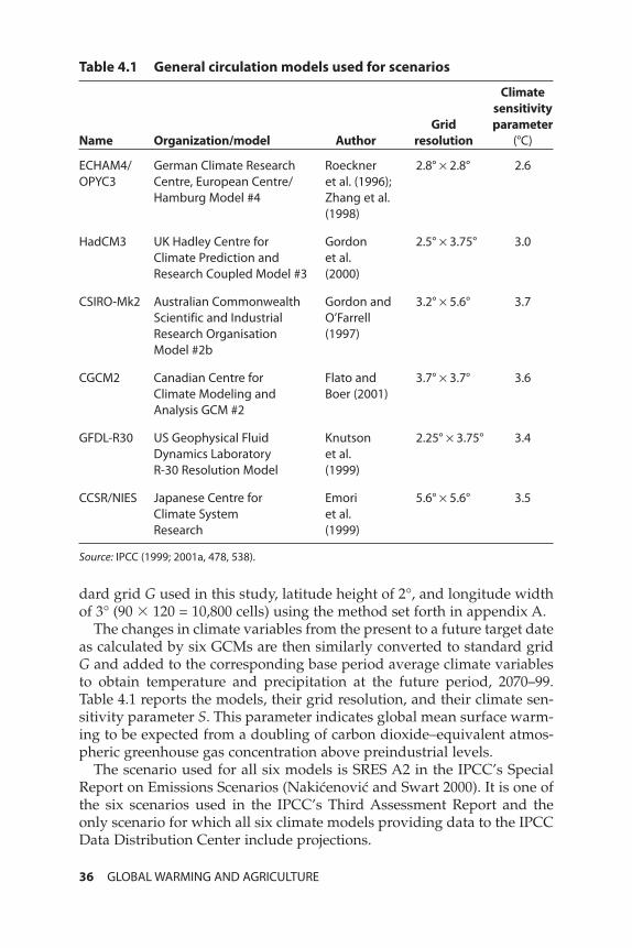
dard grid G used in this study, latitude height of 2°, and longitude widthof 3° (90 � 120 = 10,800 cells) using the method set forth in appendix A.
The changes in climate variables from the present to a future target dateas calculated by six GCMs are then similarly converted to standard gridG and added to the corresponding base period average climate variablesto obtain temperature and precipitation at the future period, 2070–99.Table 4.1 reports the models, their grid resolution, and their climate sen-sitivity parameter S. This parameter indicates global mean surface warm-ing to be expected from a doubling of carbon dioxide–equivalent atmos-pheric greenhouse gas concentration above preindustrial levels.
The scenario used for all six models is SRES A2 in the IPCC’s SpecialReport on Emissions Scenarios (Nakicenovic and Swart 2000). It is one ofthe six scenarios used in the IPCC’s Third Assessment Report and theonly scenario for which all six climate models providing data to the IPCCData Distribution Center include projections.
36 GLOBAL WARMING AND AGRICULTURE
Table 4.1 General circulation models used for scenarios
Climatesensitivity
Grid parameterName Organization/model Author resolution (°C)
ECHAM4/ German Climate Research Roeckner 2.8° × 2.8° 2.6OPYC3 Centre, European Centre/ et al. (1996);
Hamburg Model #4 Zhang et al.(1998)
HadCM3 UK Hadley Centre for Gordon 2.5° × 3.75° 3.0Climate Prediction and et al.Research Coupled Model #3 (2000)
CSIRO-Mk2 Australian Commonwealth Gordon and 3.2° × 5.6° 3.7Scientific and Industrial O’FarrellResearch Organisation (1997)Model #2b
CGCM2 Canadian Centre for Flato and 3.7° × 3.7° 3.6Climate Modeling and Boer (2001)Analysis GCM #2
GFDL-R30 US Geophysical Fluid Knutson 2.25° × 3.75° 3.4Dynamics Laboratory et al.R-30 Resolution Model (1999)
CCSR/NIES Japanese Centre for Emori 5.6° × 5.6° 3.5Climate System et al.Research (1999)
Source: IPCC (1999; 2001a, 478, 538).
01--Chs. 1-7--1-98 6/28/07 1:19 PM Page 36
Among the six scenarios considered by the Third and Fourth AssessmentReports of the IPCC, scenario A2 was the next to highest.2 This scenarioprojects carbon emissions from all anthropogenic sources to rise from 7.3gigatons of carbon (GtC) in 1990 to 17.4 GtC by 2050 and 29.1 GtC by 2100.As argued in Cline (2004, 14), two of the six scenarios (A1T and B1) haveimplausible declines in carbon intensity of energy and are inconsistentwith a baseline with no policy incentive to reducing carbon dioxide emis-sions. In addition carbon intensity of energy could well rise later this cen-tury from the more rapid exhaustion of natural gas and oil supplies than ofabundant coal supplies, in view of the higher carbon intensity of energyfrom coal. As a result, scenario A2 should be seen more as an intermediatepath among those that are realistic than as a high emissions baseline.
It is also important to ask whether the climate models available for thisstudy have any particular bias toward over- or understatement of futureclimate change. The climate sensitivity parameter (S) of the model is thebest gauge for this question. The average sensitivity parameter in the sixGCMs applied in this study is S = 3.3°C (table 4.1). In comparison, the2007 Fourth Assessment Report of the IPCC reported that the climate sen-sitivity parameter “is likely to be in the range 2 to 4.5°C with a bestestimate of about 3°C” (IPCC 2007a, 12). So the GCMs used are close tothe standard norm for the climate sensitivity parameter.
Country-Level Climate Results: Present Day and for 2070–99
The present and future climate estimates are calculated at the level of eachof the approximately 2,800 land-based cells in the standardized grid.3
Table 4.2 reports the result of averaging these estimates at the level of 116individual countries (68), regions (10), or subzones for the seven largestcountries (38). Definitions of the multicountry regions and large-countrysubzones are in appendix D. Development of the estimates for agricul-tural land and output within each subzone of the large countries is dis-cussed in appendix E.
Tables H.1 through H.4 in appendix H report the corresponding monthlyaverage values for present and future temperatures and precipitation.Monthly detail is needed to implement several of the country- or region-specific Ricardian agricultural impact functions used in this study (seechapter 5).
COUNTRY-LEVEL CLIMATE PROJECTIONS 37
2. Cumulative anthropogenic carbon emissions from 2000 through 2100, including from de-forestation, were as follows, by scenario: A1B, 1,430 GtC; A1T, 986 GtC; A1F1, 2,107 GtC; A2,1,780 GtC; B1, 901 GtC; B2, 1,081 GtC (calculated from IPCC 2001a, 801).
3. The standardized grid contains 10,800 cells (90 x 120). The mapping of base to futureclimate is first done at the 1º � 1º grid level, which corresponds to 180 � 360 = 64,800 cells.There are 22,156 land-based cells at that resolution.
01--Chs. 1-7--1-98 6/28/07 1:19 PM Page 37

38 GLOBAL WARMING AND AGRICULTURE
Table 4.2 Present and future climate: Average temperature andprecipitation (°C and mm per day, annual averages)
Temperature Precipitation
Present, Future, Present, Future,Country 1961–90 2070–99 1961–90 2070–99
Afghanistan 13.10 18.75 0.86 0.86Algeria 22.67 27.81 0.22 0.23Angola 21.52 25.53 2.75 2.62Argentina 14.65 17.89 1.63 1.66Australia
Southeast 16.68 20.27 1.66 1.61Southwest 18.35 21.75 0.79 0.65Central East 22.02 26.10 1.59 1.61Central West 23.49 27.63 0.81 0.75North 26.38 30.04 2.55 2.55
Bangladesh 24.46 28.13 6.42 7.04Belgium 9.62 13.72 2.23 2.27Brazil
Amazon 26.04 30.38 5.97 5.84Northeast 25.58 29.46 3.58 3.52South 22.04 25.90 3.98 4.15
Burkina Faso 28.16 32.38 2.12 2.29Cambodia 26.64 29.99 5.31 5.21Cameroon 24.60 28.16 4.36 4.50Canada
Arctic –15.09 –7.28 0.46 0.78Central –0.47 5.41 1.21 1.41Northwest Territories –8.88 –2.42 0.82 1.21Pacific Coast 0.79 5.40 2.17 2.54Southeast –0.93 5.42 2.26 2.56
Central America 24.23 27.76 6.51 6.18Central Europe 7.67 12.54 2.39 2.35Chile 9.01 11.91 1.52 1.43China
Beijing Northeast 2.73 8.89 1.32 1.57Central 9.49 14.48 2.03 2.43Hong Kong Southeast 18.78 22.67 4.47 4.82Northwest 6.06 12.08 0.37 0.44South Central 17.50 21.27 3.59 3.95Tibetan Plateau –1.45 4.15 1.13 1.53Yellow Sea 14.59 19.25 2.77 3.12
Colombia 24.31 27.81 7.25 7.44Cuba 25.25 28.19 3.57 3.50Democratic Republic 23.95 27.93 4.21 4.27
of the CongoEcuador 22.15 25.36 5.52 6.01
(table continues next page)
01--Chs. 1-7--1-98 6/28/07 1:19 PM Page 38
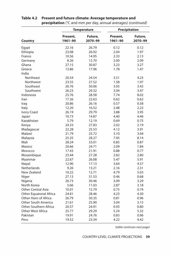
COUNTRY-LEVEL CLIMATE PROJECTIONS 39
Egypt 22.16 26.79 0.12 0.12Ethiopia 23.08 26.92 2.04 1.97France 10.56 14.95 2.33 2.13Germany 8.26 12.70 2.00 2.09Ghana 27.15 30.87 3.23 3.27Greece 13.86 17.96 1.78 1.47India
Northeast 20.54 24.54 3.51 4.23Northwest 23.55 27.52 1.58 1.97Southeast 26.76 30.06 3.05 3.42Southwest 26.23 29.32 3.04 3.47
Indonesia 25.76 28.58 7.74 8.02Iran 17.26 22.63 0.62 0.62Iraq 20.86 26.16 0.57 0.58Italy 12.20 16.52 2.48 2.23Ivory Coast 26.19 29.79 3.88 3.95Japan 10.73 14.87 4.40 4.46Kazakhstan 5.79 12.19 0.69 0.75Kenya 24.33 27.83 2.02 2.19Madagascar 22.28 25.53 4.12 3.91Malawi 21.79 25.72 3.10 3.04Malaysia 25.35 28.27 7.95 8.14Mali 28.24 33.01 0.85 0.87Mexico 20.66 24.71 2.09 1.84Morocco 17.43 21.91 0.88 0.77Mozambique 23.44 27.28 2.82 2.80Myanmar 22.67 26.08 5.47 5.91Nepal 12.90 17.13 3.64 4.57Netherlands 9.26 13.21 2.16 2.31New Zealand 10.22 12.71 4.79 5.03Niger 27.13 31.53 0.46 0.68Nigeria 26.73 30.46 3.09 3.29North Korea 5.66 11.03 2.87 3.18Other Central Asia 10.01 15.79 0.75 0.74Other Equatorial Africa 24.81 28.46 4.23 4.30Other Horn of Africa 26.79 30.35 0.81 0.96Other South America 21.61 25.90 3.04 3.15Other Southern Africa 20.57 24.91 0.93 0.80Other West Africa 25.77 29.29 5.24 5.32Pakistan 19.91 24.76 0.83 0.96Peru 19.52 23.34 4.22 4.42
(table continues next page)
Table 4.2 Present and future climate: Average temperature andprecipitation (°C and mm per day, annual averages) (continued)
Temperature Precipitation
Present, Future, Present, Future,Country 1961–90 2070–99 1961–90 2070–99
01--Chs. 1-7--1-98 6/28/07 1:19 PM Page 39
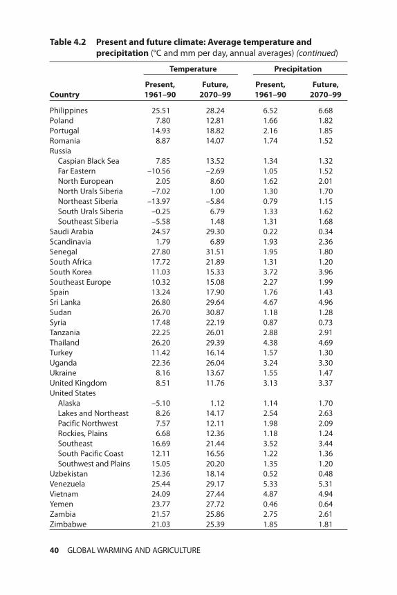
40 GLOBAL WARMING AND AGRICULTURE
Philippines 25.51 28.24 6.52 6.68Poland 7.80 12.81 1.66 1.82Portugal 14.93 18.82 2.16 1.85Romania 8.87 14.07 1.74 1.52Russia
Caspian Black Sea 7.85 13.52 1.34 1.32Far Eastern –10.56 –2.69 1.05 1.52North European 2.05 8.60 1.62 2.01North Urals Siberia –7.02 1.00 1.30 1.70Northeast Siberia –13.97 –5.84 0.79 1.15South Urals Siberia –0.25 6.79 1.33 1.62Southeast Siberia –5.58 1.48 1.31 1.68
Saudi Arabia 24.57 29.30 0.22 0.34Scandinavia 1.79 6.89 1.93 2.36Senegal 27.80 31.51 1.95 1.80South Africa 17.72 21.89 1.31 1.20South Korea 11.03 15.33 3.72 3.96Southeast Europe 10.32 15.08 2.27 1.99Spain 13.24 17.90 1.76 1.43Sri Lanka 26.80 29.64 4.67 4.96Sudan 26.70 30.87 1.18 1.28Syria 17.48 22.19 0.87 0.73Tanzania 22.25 26.01 2.88 2.91Thailand 26.20 29.39 4.38 4.69Turkey 11.42 16.14 1.57 1.30Uganda 22.36 26.04 3.24 3.30Ukraine 8.16 13.67 1.55 1.47United Kingdom 8.51 11.76 3.13 3.37United States
Alaska –5.10 1.12 1.14 1.70Lakes and Northeast 8.26 14.17 2.54 2.63Pacific Northwest 7.57 12.11 1.98 2.09Rockies, Plains 6.68 12.36 1.18 1.24Southeast 16.69 21.44 3.52 3.44South Pacific Coast 12.11 16.56 1.22 1.36Southwest and Plains 15.05 20.20 1.35 1.20
Uzbekistan 12.36 18.14 0.52 0.48Venezuela 25.44 29.17 5.33 5.31Vietnam 24.09 27.44 4.87 4.94Yemen 23.77 27.72 0.46 0.64Zambia 21.57 25.86 2.75 2.61Zimbabwe 21.03 25.39 1.85 1.81
Table 4.2 Present and future climate: Average temperature andprecipitation (°C and mm per day, annual averages) (continued)
Temperature Precipitation
Present, Future, Present, Future,Country 1961–90 2070–99 1961–90 2070–99
01--Chs. 1-7--1-98 6/28/07 1:19 PM Page 40

As a first step in thinking about the agricultural implications of the cli-mate projections, it is useful to keep in mind the turning point identifiedby Mendelsohn et al. (2000, 558) beyond which additional warming hasnegative effects. They place this optimal temperature at 11.7°C in their re-duced form statistical equation for process-based crop model results, andat 14.2°C in their Ricardian model based on cross-section statistical esti-mates. Even if the more optimistic (higher) threshold is used, it turns outthat already in the present climate 62 developing countries, developingregions, or developing-country subzones are above this level, and only 25(of which 7 are in Russia) are below it. In India, for example, all four sub-zones are well above the optimal level (with the lowest average annualtemperature being for the Northeast at 20.54°C). In China, 3 of the 7 sub-zones are above the 14.2°C optimum level.
In contrast, for industrial countries, regions, or subzones, only 7 arepresently at temperatures above the optimum (5 in Australia and 2 in theUnited States) whereas 22 are below it. Broadly, then, data on the presentclimate indicate that the bulk of the developing world is already at tem-peratures that exceed optimal levels for agriculture. For these countries,further global warming would reduce agricultural production capacity. Formany countries already well above the optimal temperature level, this de-terioration could be severe, because the relationship is nonlinear with thenegative impact rising with the square of temperature, as discussed later.These data similarly suggest that if an initial phase of warming would ben-efit rather than harm agriculture, it would primarily be to the advantage ofindustrial countries and disadvantage of developing countries.
It is useful to consider the global nonocean averages for present and fu-ture temperatures and precipitation based on the estimates of table 4.2.For this purpose, each entry in the table can be weighted by its share inglobal land area or global farm area, respectively, from appendix table E.1.The results of this weighting are shown in table 4.3.
Using broadly the same climate models and the same scenario (SRESA2), the IPCC (2001a, 527) places the change in global mean temperaturefrom 1961–90 to 2070–99 at an average of 3.0°C and a range of 1.3°C to4.5°C. The higher warming found here for land areas, 4.95°C weighting byland area and 4.43°C by farm area, reflects the fact that realized surfacewarming by a given future date is expected to be greater over land thanfor the oceans.4 Actual warming to date from 1950 to 1993 for land surfaceair temperature has been about twice that for sea surface air temperature(IPCC 2001a, 26). This is an important distinction for exercises examiningagricultural impact in response to temperature change, because it meansthat the relevant temperature change for agriculture will be higher thanthe change in global mean temperature including the oceans.
COUNTRY-LEVEL CLIMATE PROJECTIONS 41
4. “Generally, the land warms faster than the ocean, the land warms more than the ocean afterforcing stabilizes, and there is greater relative warming at high latitudes” (IPCC 2001a, 528).
01--Chs. 1-7--1-98 6/28/07 1:19 PM Page 41
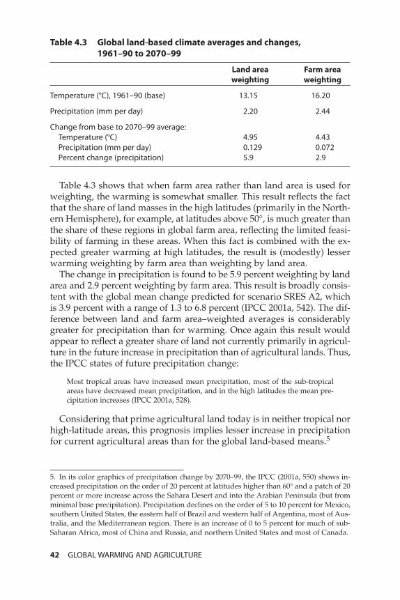
Table 4.3 shows that when farm area rather than land area is used forweighting, the warming is somewhat smaller. This result reflects the factthat the share of land masses in the high latitudes (primarily in the North-ern Hemisphere), for example, at latitudes above 50°, is much greater thanthe share of these regions in global farm area, reflecting the limited feasi-bility of farming in these areas. When this fact is combined with the ex-pected greater warming at high latitudes, the result is (modestly) lesserwarming weighting by farm area than weighting by land area.
The change in precipitation is found to be 5.9 percent weighting by landarea and 2.9 percent weighting by farm area. This result is broadly consis-tent with the global mean change predicted for scenario SRES A2, whichis 3.9 percent with a range of 1.3 to 6.8 percent (IPCC 2001a, 542). The dif-ference between land and farm area–weighted averages is considerablygreater for precipitation than for warming. Once again this result wouldappear to reflect a greater share of land not currently primarily in agricul-ture in the future increase in precipitation than of agricultural lands. Thus,the IPCC states of future precipitation change:
Most tropical areas have increased mean precipitation, most of the sub-tropicalareas have decreased mean precipitation, and in the high latitudes the mean pre-cipitation increases (IPCC 2001a, 528).
Considering that prime agricultural land today is in neither tropical norhigh-latitude areas, this prognosis implies lesser increase in precipitationfor current agricultural areas than for the global land-based means.5
42 GLOBAL WARMING AND AGRICULTURE
5. In its color graphics of precipitation change by 2070–99, the IPCC (2001a, 550) shows in-creased precipitation on the order of 20 percent at latitudes higher than 60° and a patch of 20percent or more increase across the Sahara Desert and into the Arabian Peninsula (but fromminimal base precipitation). Precipitation declines on the order of 5 to 10 percent for Mexico,southern United States, the eastern half of Brazil and western half of Argentina, most of Aus-tralia, and the Mediterranean region. There is an increase of 0 to 5 percent for much of sub-Saharan Africa, most of China and Russia, and northern United States and most of Canada.
Table 4.3 Global land-based climate averages and changes,1961–90 to 2070–99
Land area Farm area weighting weighting
Temperature (°C), 1961–90 (base) 13.15 16.20
Precipitation (mm per day) 2.20 2.44
Change from base to 2070–99 average:Temperature (°C) 4.95 4.43Precipitation (mm per day) 0.129 0.072Percent change (precipitation) 5.9 2.9
01--Chs. 1-7--1-98 6/28/07 1:19 PM Page 42

5Country-Level AgriculturalImpact Estimates
This chapter sets forth the method and results for this study’s country-level estimates of the potential effect of global warming by the 2080s onagriculture. The chapter first reviews the two main families of models:Ricardian and crop models. It then specifically examines a series of agri-cultural impact models, beginning with estimates by Mendelsohn andSchlesinger (1999) reflecting both of the alternative schools, then turningto a series of Ricardian country or regional model estimates, and con-cluding with the principal set of crop model estimates (Rosenzweig andIglesias 2006). The analysis applies detailed climate projections to the var-ious agricultural impact models to develop a set of alternative impact es-timates. It then arrives at a set of preferred estimates, applying judgmen-tal weighting of estimates by likely reliability. With preferred estimates inhand from the array of models without taking carbon fertilization into ac-count, the analysis then incorporates this study’s preferred quantificationof carbon fertilization.
Mendelsohn-Schlesinger Agricultural Response Functions
It is useful to begin the review of agricultural impact models with the twosummary statistical models, reduced form and cross section, provided byMendelsohn and Schlesinger (1999), or MS, because their two alternativemodels reflect, respectively, the crop model and the Ricardian model ap-proach. The reduced form, process-based model is derived from a sum-mary statistical estimate based on underlying results from an agronomicmodel of crop growth and a linear-programming model of US farms (in
43
01--Chs. 1-7--1-98 6/28/07 1:19 PM Page 43
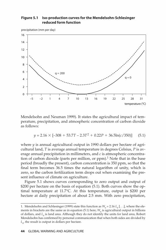
Mendelsohn and Neuman 1999). It states the agricultural impact of tem-perature, precipitation, and atmospheric concentration of carbon dioxideas follows:
y = 2.16 � [–308 � 53.7T – 2.3T2 � 0.22P � 36.5ln(c/350)] (5.1)
where y is annual agricultural output in 1990 dollars per hectare of agri-cultural land, T is average annual temperature in degrees Celsius, P is av-erage annual precipitation in millimeters, and c is atmospheric concentra-tion of carbon dioxide (parts per million, or ppm).1 Note that in the baseperiod (broadly the present), carbon concentration is 350 ppm, so that thefinal term becomes 36.5 times the natural logarithm of unity, which iszero, so the carbon fertilization term drops out when examining the pre-sent influence of climate on agriculture.
Figure 5.1 shows curves corresponding to zero output and output of$200 per hectare on the basis of equation (5.1). Both curves show the op-timal temperature at 11.7°C. At this temperature, output is $200 perhectare at daily precipitation of about 2.5 mm. With zero precipitation,
44 GLOBAL WARMING AND AGRICULTURE
1. Mendelsohn and Schlesinger (1999) state this function as Wa = 2.16 La [. . .], where the ele-ments in brackets are the same as in equation (5.1) here; Wa is agricultural output in billionsof dollars, and La is land area. Although they do not identify the units for land area, RobertMendelsohn has confirmed by personal communication that when both sides are divided byLa, the result is output in dollars per hectare.
Figure 5.1 Iso-production curves for the Mendelsohn-Schlesinger reduced form function
precipitation (mm per day)
q = 200q = 0
temperature (°C)
0
2
4
6
8
10
12
14
16
–5 –2 741 10 13 16 19 25 2822 31
01--Chs. 1-7--1-98 6/28/07 1:19 PM Page 44
output is zero even at this optimal temperature. At higher temperatures,more precipitation is required to keep productive potential positive. Forexample, at average temperature of 22°C, output would be zero if pre-cipitation were only 3 mm per day. Output of $200 per hectare would re-quire precipitation of 5.5 mm per day at this temperature. In comparison,present-day averages for the south of Brazil are 22°C and 4 mm per day(table 4.2), placing it above the zero curve but below the $200 curve.
In principle the MS reduced form model takes account of the potentialfor adaptation. As the authors state, “The analysis improves upon earlierstudies . . . by adding fruits and vegetables (not just cereals), includinglivestock, and exploring farm adaptation” (Mendelsohn and Schlesinger1999, 363). The underlying study (Adams et al. 1999) on which the MSfunction is based emphasizes that the improved models used take accountof the scope for shifting crop mixes from corn, wheat, and soybeans tomore heat-tolerant crops such as cotton, sorghum, fruits, and vegetables.That study also further takes account of adaptation through incorporatingsuch adjustments as changes in fertilizer, irrigation, and timing of plantingand harvesting (Adams et al. 1999, 18–20). It observes in broad terms that
a reasonable first approximation is that adaptation could potentially offsetroughly half of the negative impacts of a moderate climate change. However, theevidence suggests that adjustment possibilities are smaller for larger temperaturechanges (p. 32).
Mendelsohn and Schlesinger (1999) also present a cross-section or Ri-cardian agricultural impact function. This model was an early entry in anow relatively long series of studies that trace their lineage to Mendel-sohn, Nordhaus, and Shaw (1994), as noted in chapter 2.
The cross-section Ricardian function identified in Mendelsohn andSchlesinger (1999) is
v = r � g � [–475.5 � 223.2T –7.87T2 � 0.063P (5.2)– 0.000026P2 � 480ln(c/350)]
where r is the interest rate and g is a factor for the growth rate of agri-cultural output, set at 0.03 and 1.02, respectively.2 In the cross-sectionfunction, the value in brackets is the capital value of land per hectare;multiplying it by the interest rate yields the estimated rental equivalentopportunity cost of land per hectare, v, in dollars per hectare. In principlethis amount should be significantly smaller than the output value perhectare in the reduced form (equation 5.1), because it is only the land fac-tor share of output rather than total output.
COUNTRY-LEVEL AGRICULTURAL IMPACT ESTIMATES 45
2. These parameter values were clarified in a personal communication with Mendelsohn,July 15, 2006.
01--Chs. 1-7--1-98 6/28/07 1:19 PM Page 45
Mendelsohn, Morrison, Schlesinger, and Andronova (2000), or MMSA,also present versions of equations (5.1) and (5.2) with slightly modifiedparameter values. However, the set of equations in this second study per-forms less well in predicting actual base-period agricultural productivitythan the Mendelsohn and Schlesinger (1999) equations, which are appliedin the estimates in appendix F.3
Mendelsohn-Schlesinger Estimates for the United States
Appendix F develops the application of the MS models to obtain compre-hensive country-specific estimates of the agricultural impact of climatechange. Because the models are based on the United States, the results areof most direct relevance only for the United States. Nonetheless, as dis-cussed later, the MS model will be applied as the default version for theRicardian estimate when no region- or country-specific model is other-wise available. For the United States, the MS models when applied to thefuture climate estimates of the present study yield the results shown intable 5.1 for the case without carbon fertilization (see appendix F for morecomplete discussion).
The reduced form crop model specifies the dependent variable directlyas output per hectare. However, the Ricardian model generates an esti-mate of land rental equivalent per hectare. For the latter, it is necessary totranslate the percent change in land rental equivalent into a correspond-ing expected change for output. This step is ambiguous. One can certainlyconceive of land value (or land rental value) changes that translate di-rectly to corresponding proportionate changes in output potential. If a nu-clear explosion were to contaminate a land area and make it unusable fordecades, its land value would go to zero and so would its output poten-tial. For less extreme changes, however, the output potential change willbe only a fraction of the percentage change in land rental value. From onestandpoint, it will simply be the factor share of land multiplied by the per-cent change in land rental value. From another standpoint, in principlecompatible with the first, the percent change in output potential will bethe percent change in land rental value multiplied by the ratio of net rev-enue to total output, because land value is the capitalized value of net rev-enue. The final column in table 5.1 estimates the percent change in outputpotential in the Ricardian model by multiplying the percent change in
46 GLOBAL WARMING AND AGRICULTURE
3. For the 116 countries, regions, or subzones, the reduced form equation in Mendelsohnand Schlesinger (1999) yields negative predicted base output in 53 percent of the cases,whereas the MMSA (2000) reduced form equation produces negative base output in 63 per-cent of the cases. The two studies both yield 22 percent negative base output cases for thecross-section model.
01--Chs. 1-7--1-98 6/28/07 1:19 PM Page 46
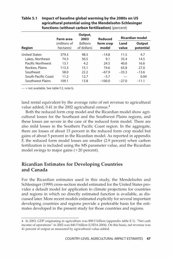
land rental equivalent by the average ratio of net revenue to agriculturalvalue added, 0.41 in the 2002 agricultural census.4
Both the reduced form crop model and the Ricardian model show agri-cultural losses for the Southeast and the Southwest Plains regions, andthese losses are severe in the case of the reduced form model. There arealso mild losses in the Southern Pacific Coast region. In the aggregate,there are losses of about 15 percent in the reduced form crop model butgains of about 5 percent in the Ricardian model. As reported in appendixF, the reduced form model losses are smaller (2.9 percent) when carbonfertilization is included using the MS parameter value, and the Ricardianmodel swings to major gains (�20 percent).
Ricardian Estimates for Developing Countries and Canada
For the Ricardian estimates used in this study, the Mendelsohn andSchlesinger (1999) cross-section model estimated for the United States pro-vides a default model for application to climate projections for countriesand regions in which no directly estimated function is available, as dis-cussed later. More recent models estimated explicitly for several importantdeveloping countries and regions provide a preferable basis for the esti-mates developed in the present study for those countries and regions.
COUNTRY-LEVEL AGRICULTURAL IMPACT ESTIMATES 47
4. In 2003, GDP originating in agriculture was $98.5 billion (appendix table E.1). “Net cashincome of operations” in 2002 was $40.5 billion (USDA 2004). On this basis, net revenue was41 percent of output as measured by agricultural value added.
Table 5.1 Impact of baseline global warming by the 2080s on USagricultural potential using the Mendelsohn-Schlesingerfunctions (without carbon fertilization) (percent)
Output,Farm area 2003 Reduced Ricardian model
(millions of (billions form crop Land OutputRegion hectares) of dollars) model value potential
United States 379.3 98.5 –14.8 11.5 4.7Lakes, Northeast 74.3 30.5 9.1 35.4 14.5Pacific Northwest 13.1 4.2 24.5 40.6 16.6Rockies, Plains 113.3 15.1 74.6 65.8 27.0Southeast 58.0 22.2 –67.9 –33.3 –13.6South Pacific Coast 11.2 12.7 –5.7 — 0.04Southwest Plains 109.1 13.8 –100.0 –27.0 –11.1
— = not available. See table F.2, note b.
01--Chs. 1-7--1-98 6/28/07 1:19 PM Page 47
Mendelsohn, Dinar, and Sanghi (2001) provide estimates for India; Ku-rukulasuriya et al. (2006) provide estimates for Africa; and a series ofstudies sponsored by the World Bank provide new estimates for majorLatin American countries (see appendix G).5 For all three sets of estimates,the model structure is as follows:
z = Σi [�iTi �βiTi2 � γiPi �δiPi
2] � K (5.3)
where z is the measure of agricultural productivity (net revenue perhectare for Africa, natural logarithm of net revenue per hectare for India,and land value per hectare for the Latin American studies), T is averagetemperature, P is average monthly precipitation, i refers to the season,and K is a composite variable that reflects the regression constant as wellas the influence of other control variables in the particular model esti-mated.6 The impact of business as usual global warming through the2080s is then obtained using this equation to estimate the difference be-tween agricultural productivity using the base period (1961–90) and fu-ture period (2070–99) climate estimates of this study. Application of thesemodels requires applying the relevant seasonal monthly averages for fu-ture temperature and precipitation from the climate models, rather thanthe annual averages. The effect of carbon fertilization is not incorporatedin these regional Ricardian estimates and must be added subsequently toobtain the overall impact of future climate change.
It is necessary to translate the change in net revenue from climatechange to the corresponding percent change in output from the base levelof output. In principle the change in net revenue will be the same in ab-solute terms as the change in output.7 In order to estimate this change as
48 GLOBAL WARMING AND AGRICULTURE
5. Note that the Mendelsohn, Dinar, and Sanghi (2001) study also provides a model forBrazil. However, application of the model results in estimates of complete shutdown of agri-culture from global warming, which as in the Brazil finding with the MS functions strainscredibility. In part because of ambiguities in the data (including nonavailability of averageland price for the study), the more recent World Bank study for Brazil is used instead as thepreferred estimate for that country, as discussed later.
6. Note, however, that in the India model, the underlying variables are expressed as differ-ences from their means (for example, T-T, for temperature, or (T-T)2, for temperaturesquared, where T is base average temperature). This approach has the property that the co-efficient on the linear term shows the marginal impact of the climate variable (e.g., temper-ature), because the square term causes symmetric damage for either a rise or a decline intemperature and has a marginal impact of zero at the original base temperature, where theinfluence of an increase in temperature is shifting from positive to negative. In contrast, inthe Africa and Latin America models, the levels rather than differences from means are theunderlying variables.
7. That is, NR = Q – Σi Xi, where NR is net revenue per hectare and Xi is the amount of pur-chased input i per hectare (mainly hired labor and fertilizer). With such inputs held constant,a yield shock from climate change translates directly into the same change in net revenue:�NR = �Q.
01--Chs. 1-7--1-98 6/28/07 1:19 PM Page 48
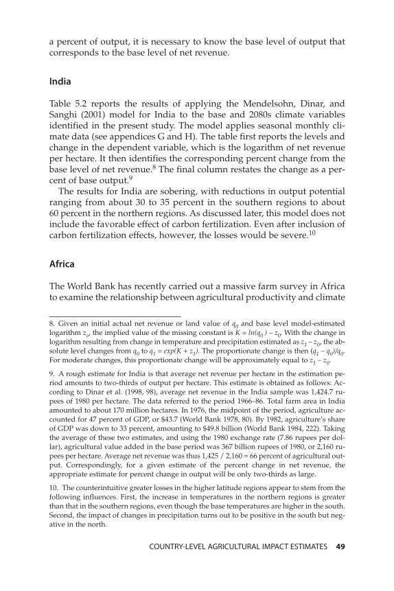
a percent of output, it is necessary to know the base level of output thatcorresponds to the base level of net revenue.
India
Table 5.2 reports the results of applying the Mendelsohn, Dinar, andSanghi (2001) model for India to the base and 2080s climate variablesidentified in the present study. The model applies seasonal monthly cli-mate data (see appendices G and H). The table first reports the levels andchange in the dependent variable, which is the logarithm of net revenueper hectare. It then identifies the corresponding percent change from thebase level of net revenue.8 The final column restates the change as a per-cent of base output.9
The results for India are sobering, with reductions in output potentialranging from about 30 to 35 percent in the southern regions to about 60 percent in the northern regions. As discussed later, this model does notinclude the favorable effect of carbon fertilization. Even after inclusion ofcarbon fertilization effects, however, the losses would be severe.10
Africa
The World Bank has recently carried out a massive farm survey in Africato examine the relationship between agricultural productivity and climate
COUNTRY-LEVEL AGRICULTURAL IMPACT ESTIMATES 49
8. Given an initial actual net revenue or land value of q0 and base level model-estimatedlogarithm zo, the implied value of the missing constant is K = ln(q0 ) – z0. With the change inlogarithm resulting from change in temperature and precipitation estimated as z1 – z0, the ab-solute level changes from q0 to q1 = exp(K + z1). The proportionate change is then (q1 – q0)/q0.For moderate changes, this proportionate change will be approximately equal to z1 – z0.
9. A rough estimate for India is that average net revenue per hectare in the estimation pe-riod amounts to two-thirds of output per hectare. This estimate is obtained as follows: Ac-cording to Dinar et al. (1998, 98), average net revenue in the India sample was 1,424.7 ru-pees of 1980 per hectare. The data referred to the period 1966–86. Total farm area in Indiaamounted to about 170 million hectares. In 1976, the midpoint of the period, agriculture ac-counted for 47 percent of GDP, or $43.7 (World Bank 1978, 80). By 1982, agriculture’s shareof GDP was down to 33 percent, amounting to $49.8 billion (World Bank 1984, 222). Takingthe average of these two estimates, and using the 1980 exchange rate (7.86 rupees per dol-lar), agricultural value added in the base period was 367 billion rupees of 1980, or 2,160 ru-pees per hectare. Average net revenue was thus 1,425 / 2,160 = 66 percent of agricultural out-put. Correspondingly, for a given estimate of the percent change in net revenue, theappropriate estimate for percent change in output will be only two-thirds as large.
10. The counterintuitive greater losses in the higher latitude regions appear to stem from thefollowing influences. First, the increase in temperatures in the northern regions is greaterthan that in the southern regions, even though the base temperatures are higher in the south.Second, the impact of changes in precipitation turns out to be positive in the south but neg-ative in the north.
01--Chs. 1-7--1-98 6/28/07 1:19 PM Page 49
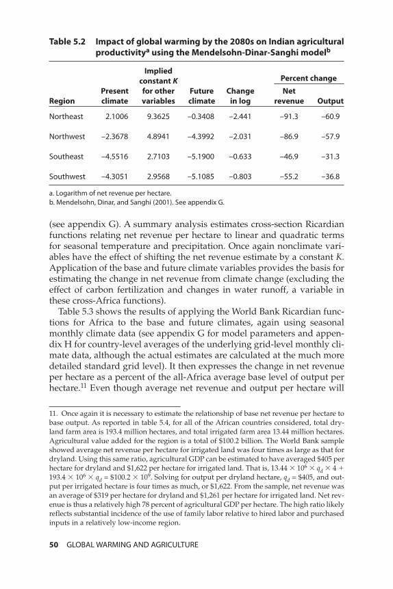
(see appendix G). A summary analysis estimates cross-section Ricardianfunctions relating net revenue per hectare to linear and quadratic termsfor seasonal temperature and precipitation. Once again nonclimate vari-ables have the effect of shifting the net revenue estimate by a constant K.Application of the base and future climate variables provides the basis forestimating the change in net revenue from climate change (excluding theeffect of carbon fertilization and changes in water runoff, a variable inthese cross-Africa functions).
Table 5.3 shows the results of applying the World Bank Ricardian func-tions for Africa to the base and future climates, again using seasonalmonthly climate data (see appendix G for model parameters and appen-dix H for country-level averages of the underlying grid-level monthly cli-mate data, although the actual estimates are calculated at the much moredetailed standard grid level). It then expresses the change in net revenueper hectare as a percent of the all-Africa average base level of output perhectare.11 Even though average net revenue and output per hectare will
50 GLOBAL WARMING AND AGRICULTURE
11. Once again it is necessary to estimate the relationship of base net revenue per hectare tobase output. As reported in table 5.4, for all of the African countries considered, total dry-land farm area is 193.4 million hectares, and total irrigated farm area 13.44 million hectares.Agricultural value added for the region is a total of $100.2 billion. The World Bank sampleshowed average net revenue per hectare for irrigated land was four times as large as that fordryland. Using this same ratio, agricultural GDP can be estimated to have averaged $405 perhectare for dryland and $1,622 per hectare for irrigated land. That is, 13.44 � 106 � qd � 4 �193.4 � 106 � qd = $100.2 � 109. Solving for output per dryland hectare, qd = $405, and out-put per irrigated hectare is four times as much, or $1,622. From the sample, net revenue wasan average of $319 per hectare for dryland and $1,261 per hectare for irrigated land. Net rev-enue is thus a relatively high 78 percent of agricultural GDP per hectare. The high ratio likelyreflects substantial incidence of the use of family labor relative to hired labor and purchasedinputs in a relatively low-income region.
Table 5.2 Impact of global warming by the 2080s on Indian agriculturalproductivitya using the Mendelsohn-Dinar-Sanghi modelb
Impliedconstant K Percent change
Present for other Future Change NetRegion climate variables climate in log revenue Output
Northeast 2.1006 9.3625 –0.3408 –2.441 –91.3 –60.9
Northwest –2.3678 4.8941 –4.3992 –2.031 –86.9 –57.9
Southeast –4.5516 2.7103 –5.1900 –0.633 –46.9 –31.3
Southwest –4.3051 2.9568 –5.1085 –0.803 –55.2 –36.8
a. Logarithm of net revenue per hectare.b. Mendelsohn, Dinar, and Sanghi (2001). See appendix G.
01--Chs. 1-7--1-98 6/28/07 1:19 PM Page 50
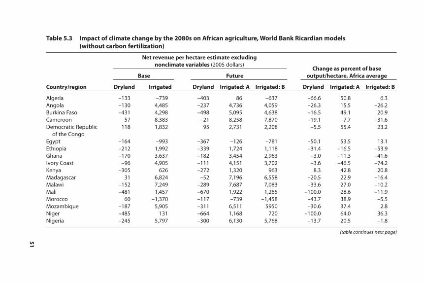
51
Table 5.3 Impact of climate change by the 2080s on African agriculture, World Bank Ricardian models(without carbon fertilization)
Net revenue per hectare estimate excludingnonclimate variables (2005 dollars)
Change as percent of baseBase Future output/hectare, Africa average
Country/region Dryland Irrigated Dryland Irrigated: A Irrigated: B Dryland Irrigated: A Irrigated: B
Algeria –133 –739 –403 86 –637 –66.6 50.8 6.3Angola –130 4,485 –237 4,736 4,059 –26.3 15.5 –26.2Burkina Faso –431 4,298 –498 5,095 4,638 –16.5 49.1 20.9Cameroon 57 8,383 –21 8,258 7,870 –19.1 –7.7 –31.6Democratic Republic 118 1,832 95 2,731 2,208 –5.5 55.4 23.2
of the CongoEgypt –164 –993 –367 –126 –781 –50.1 53.5 13.1Ethiopia –212 1,992 –339 1,724 1,118 –31.4 –16.5 –53.9Ghana –170 3,637 –182 3,454 2,963 –3.0 –11.3 –41.6Ivory Coast –96 4,905 –111 4,151 3,702 –3.6 –46.5 –74.2Kenya –305 626 –272 1,320 963 8.3 42.8 20.8Madagascar 31 6,824 –52 7,196 6,558 –20.5 22.9 –16.4Malawi –152 7,249 –289 7,687 7,083 –33.6 27.0 –10.2Mali –481 1,457 –670 1,922 1,265 –100.0 28.6 –11.9Morocco 60 –1,370 –117 –739 –1,458 –43.7 38.9 –5.5Mozambique –187 5,905 –311 6,511 5950 –30.6 37.4 2.8Niger –485 131 –664 1,168 720 –100.0 64.0 36.3Nigeria –245 5,797 –300 6,130 5,768 –13.7 20.5 –1.8
(table continues next page)
01--Chs.
1-7--1-98
6/28/07
1:19
PM
Page
51
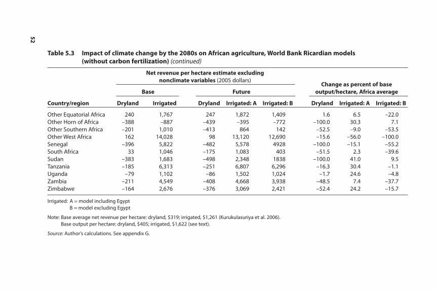
52
Other Equatorial Africa 240 1,767 247 1,872 1,409 1.6 6.5 –22.0Other Horn of Africa –388 –887 –439 –395 –772 –100.0 30.3 7.1Other Southern Africa –201 1,010 –413 864 142 –52.5 –9.0 –53.5Other West Africa 162 14,028 98 13,120 12,690 –15.6 –56.0 –100.0Senegal –396 5,822 –482 5,578 4928 –100.0 –15.1 –55.2South Africa 33 1,046 –175 1,083 403 –51.5 2.3 –39.6Sudan –383 1,683 –498 2,348 1838 –100.0 41.0 9.5Tanzania –185 6,313 –251 6,807 6,296 –16.3 30.4 –1.1Uganda –79 1,102 –86 1,502 1,024 –1.7 24.6 –4.8Zambia –211 4,549 –408 4,668 3,938 –48.5 7.4 –37.7Zimbabwe –164 2,676 –376 3,069 2,421 –52.4 24.2 –15.7
Irrigated: A = model including EgyptB = model excluding Egypt
Note: Base average net revenue per hectare: dryland, $319; irrigated, $1,261 (Kurukulasuriya et al. 2006).Base output per hectare: dryland, $405; irrigated, $1,622 (see text).
Source: Author’s calculations. See appendix G.
Table 5.3 Impact of climate change by the 2080s on African agriculture, World Bank Ricardian models(without carbon fertilization) (continued)
Net revenue per hectare estimate excludingnonclimate variables (2005 dollars)
Change as percent of baseBase Future output/hectare, Africa average
Country/region Dryland Irrigated Dryland Irrigated: A Irrigated: B Dryland Irrigated: A Irrigated: B
01--Chs.
1-7--1-98
6/28/07
1:19
PM
Page
52
vary among countries, because the parameters of the models are uniformacross all countries in the region, it is appropriate that estimated net rev-enue changes be compared with the regional average rather than country-specific output per hectare.
For irrigated agriculture, variant A is from the model reported in Ku-rukulasuriya et al. (2006) for all observations including those in Egypt,which alone accounts for 58 percent of the observations for irrigated agri-culture. The authors note that Egypt may be atypical because of the mas-sive availability of irrigation from the Nile River; indeed, there are no dry-land farms at all in the sample for Egypt. They therefore also report thekey marginal parameters for temperature and precipitation separately forthe full model including Egypt and for a model excluding Egypt, desig-nated here as A and B, respectively (see appendix G). Table 5.3 reports es-timates for model B by applying the differences in these marginal para-meters to the change in temperature and precipitation and adding theresult to the estimated change in net revenue in model A.12
There is a predominant pattern of large negative changes from businessas usual warming (excluding carbon fertilization) in dryland African agri-culture. The median change is –31 percent. In contrast, for variant A of theirrigated agriculture model (including Egypt), the median change is �24.4percent. However, when variant B of the irrigated agriculture model is ap-plied (excluding Egypt in the parameter estimation), negative results alsodominate irrigated agriculture, with the median change at –11.1 percent.
One pattern that stands out in table 5.3 is the dispersion of results.There is a high frequency of severely adverse effects for dryland agricul-ture, as five of the 28 countries or regions have complete shutdown. An-other six have reductions in agricultural capacity by about half or more.However, four countries have only modest declines averaging about 3percent, and two countries or regions have modest increases. Even so, thedominant pattern is of serious loss.
A second pattern is that several countries show major gains for irri-gated agriculture if the model heavily influenced by Egypt and its Nilewater is used (variant A), but the pattern shifts to dominant losses even inirrigated agriculture if the function omitting the Egypt observations is ap-plied (variant B).
Because the results differ substantially between dryland and irrigatedagriculture (even when variant B is used), to obtain meaningful estimatesit is necessary to weight the two types of agriculture. Table 5.4 reports the
COUNTRY-LEVEL AGRICULTURAL IMPACT ESTIMATES 53
12. That is, the full model A yields the estimates shown in the second and fourth columnsof table 5.5. The future net revenue estimate for model B is obtained by adding the follow-ing value to that in the fourth column of the table for model A: �yB – �yA = (�B – �A) �T +(�B – �A) �P, where T is temperature (degrees Celsius), P is precipitation (mm per month), yis net revenue per hectare, � refers to change from climate change, � is the marginal para-meter for temperature, and � is the marginal parameter for precipitation. The values for �Tand �P are taken from the present and future annual averages shown in table 4.2.
01--Chs. 1-7--1-98 6/28/07 1:19 PM Page 53
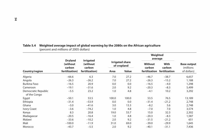
54
Table 5.4 Weighted average impact of global warming by the 2080s on the African agriculture (percent and millions of 2005 dollars)
Weighted
Dryland Irrigatedaverage
(without (without Without With Base outputcarbon carbon carbon carbon (millions
Country/region fertilization) fertilization) Area Value fertilization fertilization of dollars)
Algeria –66.6 6.3 7.0 27.2 –46.7 –38.7 6,657Angola –26.3 –26.2 7.0 27.2 –26.3 –15.2 1,188Burkina Faso –16.5 20.9 0.0 0.0 –16.5 –4.0 1,298Cameroon –19.1 –31.6 2.0 9.2 –20.3 –8.3 5,499Democratic Republic –5.5 23.2 1.0 4.8 –4.1 10.2 3,292
of the CongoEgypt –50.1 53.5 100.0 100.0 53.5 76.5 13,189Ethiopia –31.4 –53.9 0.0 0.0 –31.4 –21.2 2,748Ghana –3.0 –41.6 3.0 13.3 –8.2 5.6 2,748Ivory Coast –3.6 –74.2 1.0 4.8 –7.0 7.0 3,574Kenya 8.3 20.8 19.0 53.7 15.0 32.3 2,302Madagascar –20.5 –16.4 1.0 4.8 –20.3 –8.3 1,587Malawi –33.6 –10.2 2.0 9.2 –31.5 –21.2 651Mali –100.0 –11.9 31.0 69.0 –39.0 –29.9 1,645Morocco –43.7 –5.5 2.0 9.2 –40.1 –31.1 7,436
Irrigated shareof cropland
01--Chs.
1-7--1-98
6/28/07
1:19
PM
Page
54

55
Mozambique –30.6 2.8 5.0 20.7 –23.6 –12.1 1,122Niger –100.0 36.3 15.0 46.6 –36.1 –26.5 1,094Nigeria –13.7 –1.8 3.0 13.3 –12.1 1.1 15,180Other Equatorial Africa 1.6 –22.0 1.0 4.8 0.5 15.6 1,429Other Horn of Africa –100.0 7.1 1.0 4.8 –94.8 –94.1 20Other Southern Africa –52.5 –53.5 1.0 4.8 –52.5 –45.4 619Other West Africa –15.6 –100.0 5.0 20.7 –33.2 –23.2 1,832Senegal –100.0 –55.2 10.0 35.5 –84.0 –81.6 1,105South Africa –51.5 –39.6 11.0 38.0 –47.0 –39.0 6,395Sudan –100.0 9.5 4.0 17.1 –81.1 –78.3 6,944Tanzania –16.3 –1.1 0.0 0.0 –16.3 –3.7 4,629Uganda –1.7 –4.8 6.0 24.0 –2.5 12.1 2,016Zambia –48.5 –37.7 3.0 13.3 –47.1 –39.1 1,000Zimbabwe –52.4 –15.7 5.0 20.7 –44.7 –36.4 3,018
Total –18.6 –6.3 100,215Excluding Egypt –29.5 –18.9
Median –28.9 –18.2
Sources: Table 5.3 using non-Egypt irrigated model B except for Egypt; World Bank (2006).
01--Chs.
1-7--1-98
6/28/07
1:19
PM
Page
55
share of farm area under irrigation and the corresponding estimate of theshare of total crop value from irrigated farming in each country.13 In table5.4, the with-Egypt irrigated function is applied only for Egypt; for all oth-ers the without-Egypt function is used (variant B in table 5.3).
For each country or region, the weighted average impact of climatechange is calculated by weighting the dryland and irrigated estimates by their respective value shares in the base period. This estimate excludesthe carbon fertilization effect. When this estimate is aggregated across allAfrican countries and regions by weighting by base period agriculturaloutput, the result is that African agricultural capacity would decline by anestimated 18.6 percent by the 2080s, before taking account of carbon fertil-ization. Excluding Egypt, the decline would be about 30 percent. A com-parable set of estimates including carbon fertilization is obtained by ap-plying a uniform 15 percent enhancement of yields from this effect by the2080s, as discussed above. The result is a still substantial aggregate declineof 6.3 percent in the aggregate and about 19 percent excluding Egypt.
These averages mask greater declines in the majority of countries in the region. The weighted averages are buoyed by the highly favorable re-sults for Egypt, which has the second largest output base in the continent,and an unusually small net decline for Nigeria, which has the largest out-put base. This masking is evident in the fact that the median changes inagricultural capacity are almost identical to the output-weighted averagechanges when Egypt is excluded.
Latin America
In another recent study coordinated by the World Bank, farm sample sur-vey data were compiled and used to estimate Ricardian functions for theimpact of climate on land value per hectare. These studies also used rela-tively standardized versions of equation (5.3) above. All included equationsfor land value per hectare. Some included equations for net revenue perhectare, and some distinguished between small- and large-farm equations.
Appendix table G.3 reports the coefficients estimated in these equationsfor Argentina, Brazil, Chile, and Ecuador. The equations shown there areapplied to the detailed grid-level climate projection data of this study (av-erages of which are shown at the country level in appendix H) to estimatethe percent change in land value from business as usual global warmingby the 2080s. The results of this calculation are shown in the third columnof table 5.5. Difficulties in interpretation of variables or data values in thesource studies precluded application here of the equations estimated inthis series for Colombia and Venezuela.
56 GLOBAL WARMING AND AGRICULTURE
13. The African average net revenue per hectare in irrigated farming is about four times ashigh as that for dryland farming. The irrigated value shares are correspondingly higher thanarea shares.
01--Chs. 1-7--1-98 6/28/07 1:19 PM Page 56

The underlying studies themselves included either outright estimatesof the impact of future climate change (Argentina, Brazil, Ecuador, andVenezuela) or parametric results indicating the impact that could be ex-pected from alternative amounts of warming (2.5°C and 5°C) and changein precipitation (�10 percent; the cases of Chile and Colombia). The stud-ies used three climate models: the Parallel Climate Model (PCM), Centerfor Climate System Research (CCSR), and Climate Crisis Coalition (CCC),from Washington et al. (2000), Emori et al. (1999), and Boer, Flato, andRamsden (2000), respectively. However, they did not report the emissionsscenarios assumed or the climate projections of these models.
It is possible to take account of the climate impact estimates of the stud-ies themselves as well as the estimates obtained when applying the pre-sent study’s climate estimates to the models in these studies. For the fourstudies reporting direct impacts (labeled “A” in table 5.5), the simple av-erage agricultural impact estimate is taken across the three climate modelsand the two benchmark years 2060 and 2100 as the central estimate for2080 comparable to the estimates of the present study. In cases where thereare both small-farm and large-farm estimates, the average of both is used.In the other two studies without direct impact projections, the parametriceffects of changes in temperature and precipitation are applied to the pre-sent study’s estimate of climate change (table 4.2) to obtain the implied cli-mate impact from the underlying study (cases labeled “B” in table 5.5).
COUNTRY-LEVEL AGRICULTURAL IMPACT ESTIMATES 57
Table 5.5 Impact of global warming by the 2080s on agriculturalpotential in major Latin American countries (without carbonfertilization), World Bank studies (percent)
Implied by Model applicationAverage
underlying study: in present study: Land OutputCountry Land value Basis Land value value potential
Argentina –17.9 A 1.4 –8.2 –4.1Brazil –22.0 A 2.1 –10.1 –5.0
Amazon n.a. –76.0 –49.0 –24.5Northeast n.a. –18.0 –20.0 –10.0South n.a. 10.0 –6.0 –3.0
Chile –3.6 B –86.0 –44.8 –22.4Colombia –34.1 B n.a. –34.1 –17.0Ecuador –6.9 A –100.0 –53.5 –26.8Venezuela –75.4 A n.a. –75.4 –37.7
n.a. = not available
A = average of 2060 and 2100 results in underlying studyB = application of marginal temperature and precipitation parameters in underlying study toclimate change estimated in present study
Source: See text and appendix G.
01--Chs. 1-7--1-98 6/28/07 1:19 PM Page 57
The resulting estimates show relatively large divergence between theimpact estimates in the underlying Latin American studies and the corre-sponding estimates of the present study using their models. There is nosystematic direction of the difference, as the underlying studies show moresevere effects than the calculations in this study for Argentina and Brazilbut less severe for Chile and Ecuador. The divergences could arise becauseof divergent future climate estimates, differences between the large- andsmall-farm estimates (the models applied here are either the aggregatemodel or a weighted average), and differences in regional detail. In Brazil,in particular, the underlying study does not distinguish among regions,whereas the estimates here differentiate among three geographical zones.
Because of the fairly large divergences, the most prudent approachwould seem to be to take a simple average of the impact estimates indi-cated (directly or implied) in the underlying studies and the impact esti-mates obtained here by applying the present study’s climate projectionsto the Ricardian equations taken from these studies. This average estimateis shown in the next to last column of table 5.5.
Once again it is necessary to translate the percent change in land valuefrom the models into corresponding change in output potential. Follow-ing the discussion for US estimates above, the land factor share or ratio ofnet revenue to value added is the fraction appropriate to apply for thispurpose, with the caveat that it could understate the loss in output po-tential in extreme cases in which the land becomes essentially unusable.For Latin America, this ratio is set at 50 percent, intermediate between theUS ratio (41 percent) and the ratio for India (67 percent) in view of thelikely intermediate factor share of land at an intermediate stage of devel-opment. The final column in table 5.5 applies this fraction to arrive at theimpact on potential output.
Canada
Reinsborough (2003) has prepared Ricardian estimates for the impact of cli-mate change on agriculture in Canada. She emphasizes that this approach“presents an upper bound on the benefits of climate change” because it“assumes perfect adjustment to climate change and no costs other thanchange in land value” (pp. 22, 25). She estimates farmland value per hectareas a function of seasonal temperature, temperature squared, precipitation,and precipitation squared (for January, April, July, and October), as well ascontrol variables. When she applies the estimated coefficients to a postu-lated climate change of 2.8°C temperature increase and 8 percent increasein precipitation, she finds a negligible change in farmland values.14
Preliminary subsequent work by Mendelsohn and Reinsborough (2007)confirms that there is a statistically significant difference between Ricar-
58 GLOBAL WARMING AND AGRICULTURE
14. A total rise of only about $1 million for the whole of Canada (Reinsborough 2003, 32).
01--Chs. 1-7--1-98 6/28/07 1:19 PM Page 58
dian function estimates for Canada and those for the United States. Onthis basis, it would be misleading to use the default MS Ricardian esti-mates in appendix F for Canada. The approach adopted later will insteadsimply place the Canadian estimates in the Ricardian family at zero,based on the Reinsborough (2003) results. Because Russia is located in asimilar latitude range as Canada, the preferred estimates developed laterset climate impact effects at zero for Russia as well, because once againapplication of the default MS function could be seriously misleading.
It should be emphasized that if instead the default US-based MSRicardian model estimates were used, large gains in agricultural potentialfrom global warming would be identified for Canada and Russia (see ap-pendix F).15 Because the Reinsborough (2003) estimates are directly forCanada, however, they should be seen as strictly dominating the defaultMS estimates for that country. Note moreover that the zero-impact resultsin the Canadian study are much more consistent with the estimates forCanada from the Rosenzweig and Iglesias (2006) crop models, discussedlater.
Sensitivity to Climate Models
The spirit of this study is to apply a “consensus” projection of the busi-ness as usual climate to the agricultural response functions to obtain acentral estimate of the implications of global warming for agriculture. It isfair to ask, however, whether this approach masks an extreme degree ofvariability that would be found if each of the climate models were appliedindividually for this task. Appendix I examines the degree of dispersionof future temperature and precipitation estimates among the six climatemodels in the IPCC Data Distribution Centre (listed in table 4.1).
To examine the corresponding dispersion of estimates for agriculturalimpact, it is useful to consider the results of the standard default MSRicardian model when applied to each of the underlying climate modelsseparately. Table 5.6 reports these results for 30 major countries or regionsto provide a sense of the range of dispersion. Each of the countries in thetable is in category “a” in appendix table F.2, the category in which it is
COUNTRY-LEVEL AGRICULTURAL IMPACT ESTIMATES 59
15. The case of Russia is more ambiguous, and application of the Canadian zero-impact re-sult to Russia (rather than the default MS model) rests on the proposition that given its lati-tudinal location it resembles Canadian conditions much more than those of the UnitedStates. The US-based MS Ricardian function would instead place the impact on Russia at aremarkable 152 percent rise in agricultural capacity even without carbon fertilization, andapplying that estimate would boost the estimated global impact in table 5.8 by 0.86 percent-age point. However, such a large contribution from Russia would surely raise questions ofpolitical economy and in particular the question of “Dutch disease.” As a major energy ex-porter, Russia could well have such a strong exchange rate that its firms would not havemuch incentive to make the country a major agricultural exporter.
01--Chs. 1-7--1-98 6/28/07 1:19 PM Page 59

60
Table 5.6 Dispersion of Mendelsohn-Schlesinger Ricardian model estimates across climate models (without carbon fertilization) (percent change in land rental equivalent)
Consensus CoefficientCountry CCSR HadCM GFDL ECHAM CSIRO CGCM estimate of variation
Angola –100.0 –89.5 –67.5 –100.0 –63.4 –83.1 –84.1 0.42Argentina –20.5 –17.0 –9.8 –11.6 –15.1 –15.7 –14.8 0.57Brazil, Southern –100.0 –100.0 –67.1 –100.0 –86.8 –89.7 –99.2 0.32Chile 18.7 16.8 18.2 16.8 18.2 19.7 18.2 0.14China, Central 26.4 23.5 23.5 28.9 29.2 23.5 27.1 0.24China, South Central –47.3 –34.8 –22.2 –29.3 –26.2 –32.5 –31.4 0.61Colombia –100.0 –100.0 –100.0 –100.0 –100.0 –100.0 –100.0 0.00Germany 31.2 28.8 28.3 32.2 26.6 24.7 30.6 0.22Madagascar –95.9 –77.8 –74.1 –97.0 –70.8 –80.6 –81.6 0.30Malawi –100.0 –100.0 –68.3 –100.0 –58.1 –76.1 –84.8 0.50Mexico –100.0 –80.8 –60.3 –68.9 –53.8 –52.8 –71.8 0.59Morocco –68.9 –32.9 –23.2 –44.5 –31.6 –35.3 –38.5 0.91Mozambique –100.0 –100.0 –100.0 –100.0 –100.0 –100.0 –100.0 0.00New Zealand 6.0 10.5 11.7 11.9 10.3 11.3 10.0 0.48Peru –95.9 –100.0 –57.1 –86.3 –57.0 –59.8 –78.1 0.60Poland 33.2 35.6 32.7 38.4 33.6 32.3 37.2 0.15Portugal –27.0 –12.4 –11.0 –23.2 –10.1 –10.2 –14.7 1.07Romania 16.1 24.2 22.1 24.8 23.7 22.8 24.8 0.32Russia, Caspian Black Sea 33.8 41.0 33.9 41.9 40.1 40.0 41.1 0.21South Africa –42.4 –39.5 –32.3 –43.5 –30.5 –39.6 –37.7 0.32Syria –75.1 –38.1 –26.5 –39.2 –39.3 –37.0 –41.9 0.88Tanzania –100.0 –100.0 –77.2 –100.0 –69.8 –77.8 –95.4 0.36Turkey –7.7 2.8 5.8 4.1 3.4 5.3 3.5 4.89Uganda –100.0 –100.0 –85.2 –99.9 –74.3 –74.7 –94.9 0.32United Kingdom 26.9 18.4 22.8 25.4 21.1 18.5 23.4 0.35US Lakes and Northeast 25.9 32.9 32.8 36.9 36.1 33.3 35.4 0.26US Southeast –64.6 –34.8 –23.9 –22.6 –31.2 –31.0 –33.3 0.99Venezuela –100.0 –100.0 –100.0 –100.0 –100.0 –100.0 –100.0 0.00Zambia –100.0 –99.9 –69.1 –100.0 –67.8 –90.5 –91.3 0.39
Note: For climate models, see table 4.1.
01--Chs.
1-7--1-98
6/28/07
1:19
PM
Page
60
possible to compare the change in land rental equivalent directly againstthe model’s prediction for the base period. The table considers the casewithout carbon fertilization.
It is evident in table 5.6 that there is relatively close agreement amongthe underlying climate models in terms of the resulting agricultural im-pacts estimated for each country when applied to the MS cross-sectionmodel. The US Lakes-Northeast region, for example, generates estimateslying in a relatively narrow range, from an increase in land rental equiva-lent of about 26 percent to an increase of about 36 percent. The next to lastcolumn, labeled “consensus,” is the central estimate using the average ofthe six climate models.16 The final column reports the coefficient of varia-tion for the country.17 The median value for the coefficient of variation is0.34, indicating in rough terms that typically the variability of the esti-mates as measured by the standard deviation is some � 17 percent of theaverage estimate.18
The central message of the experiment reported in table 5.6 is that theestimates here should be relatively robust with respect to variation amongclimate models. All six models tend to agree on whether the agriculturalimpact will be substantially positive in a particular region (e.g., Germanyor Poland) or strongly negative (e.g., Colombia or Mozambique). Forsome countries and regions, alternative impact estimates in this studybased on alternative agricultural-economic models are considerably dif-ferent from those in appendix tables F.1 and F.2. The relatively close ad-herence of the various climate model estimates when applied to the sameimpact model (in the case of table 5.6, the MS Ricardian model) suggeststhat in estimating country-specific impacts, variability across the agricul-tural-economic models is more important than variability across the cli-mate models. This diagnosis also tends to support the use of the consen-sus climate model approach adopted for this study and the focus ondiffering results from differing agricultural-economic models rather thanfrom differing climate models.
Rosenzweig et al. Crop Model Results
Rosenzweig and Iglesias (2006) provide a query-based database that re-turns estimates of the impact of prospective global warming, under alter-
COUNTRY-LEVEL AGRICULTURAL IMPACT ESTIMATES 61
16. The entries in appendix table F.2 correspond to those in the final column of table 5.6 aftershrinkage to take account of the ratio of net revenue to output.
17. The coefficient of variation is calculated as the square root of the sum of squared resid-uals of each of the six estimates from the average of the six, divided by the average (and re-ported in absolute value).
18. The coefficient of variation is increasingly misleading as the average value approacheszero. The high coefficient of variation for Turkey reflects this fact.
01--Chs. 1-7--1-98 6/28/07 1:19 PM Page 61
native climate scenarios and using alternative GCMs, on four major crops:wheat, rice, coarse grains (maize, barley, and others), and soybeans. Theunderlying research was developed in the 1990s by a team of agriculturalscientists from 18 countries, who estimated compatible crop models at 125agricultural sites using consistent climate change scenarios (see Rosen-zweig et al. 1993, as discussed above; and Parry, Rosenzweig, and Liver-more 2005). The process-based dynamic crop growth models incorporatethe effects of change in temperature, precipitation, and solar radiation; theeffect of carbon fertilization from increased atmospheric concentrations ofcarbon dioxide; and crop management, particularly with respect to timingof planting and extent of fertilization and irrigation. The estimates are forthree levels of adaptation: 1) no adaptation; 2) level 1 (L1): shifts in plant-ing dates by less than one month, shifts to other available varieties andcrops, and increased irrigation using existing systems; and 3) level 2 (L2):more intensive adaptations involving higher costs, including change indate of planting by more than one month; installation of new irrigationsystems; and development of new varieties.
The GCMs and climate scenarios in the query system include three mod-els with results for equilibrium carbon concentrations of 555 ppm (doublepreindustrial levels) and two “transient” model variants for expected con-ditions by the 2080s. For the transient model used here (HadCM3, HadleyCentre for Climate Prediction and Research Coupled Model 3), the IS95ascenario is used, which is the same as the IS92a “business as usual” sce-nario in the IPCC’s Second Assessment Report of 1995.19 This scenario hasa modestly lower path of rising emissions than the SRES A2 scenario in theThird Assessment Report of 2001, used for the projections in the first partof this study (see table 4.2). Thus, by 2040 fossil fuel and industrial processemissions stand at 12.66 gigatons of carbon equivalent (GtC) in IS92a and15.01 GtC in SRES A2; by 2080 the comparison is 17.0 versus 22.97 GtC, re-spectively (IPCC 2001a, 801).
The equilibrium and transient models tend to generate relatively simi-lar results at 555 ppm equilibrium and 731 ppm transient warming.20 Thisis presumably because ocean thermal lag means the ultimate equilibriumwarming associated with any given atmospheric concentration of carbonis greater than will be observed at the date this concentration is first at-tained (see Cline 1992, 92).
62 GLOBAL WARMING AND AGRICULTURE
19. Rosenzweig and Iglesias (2006) also report results for Hadley model HadCM2. How-ever, these results show much greater divergence from the results of the other three modelsused here (GISS, GFDL, and UKMO) than do the results for HadCM3. The HadCM3 results,being more representative, are thus chosen for the analysis here. (For the regions shown intable 5.7, the sum of squared residuals of percent deviation from the average estimate fromthe other three models is 11,414 for HadCM2 but only 3,116 for HadCM3.)
20. See the color maps on the methodology page in Rosenzweig and Iglesias (2006).
01--Chs. 1-7--1-98 6/28/07 1:19 PM Page 62
Table 5.7 reports the results compiled in the Rosenzweig-Iglesias data-base for the impact of global warming by the 2080s on yields of the fourmajor grains and oilseeds, again interpreting the equilibrium 555 ppm re-sults as proxies for realized impact by the 2080s. These estimates are allfor the moderate level of adaptation (L1) and full carbon fertilization ef-fects. Analysis of the difference between results with and without carbonfertilization indicates that the Rosenzweig-Iglesias estimates place thecarbon fertilization impact at about �17 percent by the 2080s.21 This im-pact is close to the 15 percent identified above as the proper target for car-bon fertilization by this period on the basis of the recent free air concen-tration enrichment (FACE) field experiments.
Synthesis of Preferred Estimates
The two basic frameworks discussed above (Ricardian statistical models,on the one hand, and crop models on the other) provide the basis for iden-tifying a set of preferred estimates that synthesize the alternative modelresults. In the first group five studies are from the same family of modelsand even share key authors.22 The first of these, and the default model forthis framework, is Mendelsohn and Schlesinger (1999). This set of esti-mates, designated source 1, comprises the cross-section estimates in ap-pendix table F.2. As noted earlier, this model was estimated using data forthe United States. Although the model provides a basis for estimation forother countries in the absence of statistical studies specific to those coun-tries, climate responses elsewhere could be substantially different fromthose for the United States, and the ranges in temperature (especially)could extend beyond those included in the US database on which themodels were estimated. This is especially so for the tropics and other lat-itudes not represented in the United States.
The second study within the first framework is the set of estimates forAfrica developed in the World Bank study (Kurukulasuriya et al. 2006)and applied here with results shown in table 5.4. The third set of estimates
COUNTRY-LEVEL AGRICULTURAL IMPACT ESTIMATES 63
21. The Rosenzweig and Iglesias (2006) results are reported as percent change in yield fromthe base period. If we call this “a” (expressed as a proportion) for results with carbon fertil-ization and “b” without, the median for the ratio (1�a)/(1�b) across the regions shown intable 5.7 is 1.159 for GISS, 1.154 for GFDL, and 1.179 for UKMO (using comparisons for theL0 adaptation levels only, because results are not reported without carbon fertilization forthe L1 adaptation cases for these three models). For the HadCM3 model, with L1 adaptation,this ratio has a median of 1.208. Note that these implied enhancement ratios are broadly con-sistent with the crop-specific ratios reported above in the summary of Rosenzweig et al.(1993).
22. Robert Mendelsohn is coauthor of three of the four studies and a project coordinator forthe fourth (the World Bank project on Latin America). All of the Ricardian estimates, more-over, trace their origins to Mendelsohn, Nordhaus, and Shaw (1994).
01--Chs. 1-7--1-98 6/28/07 1:19 PM Page 63
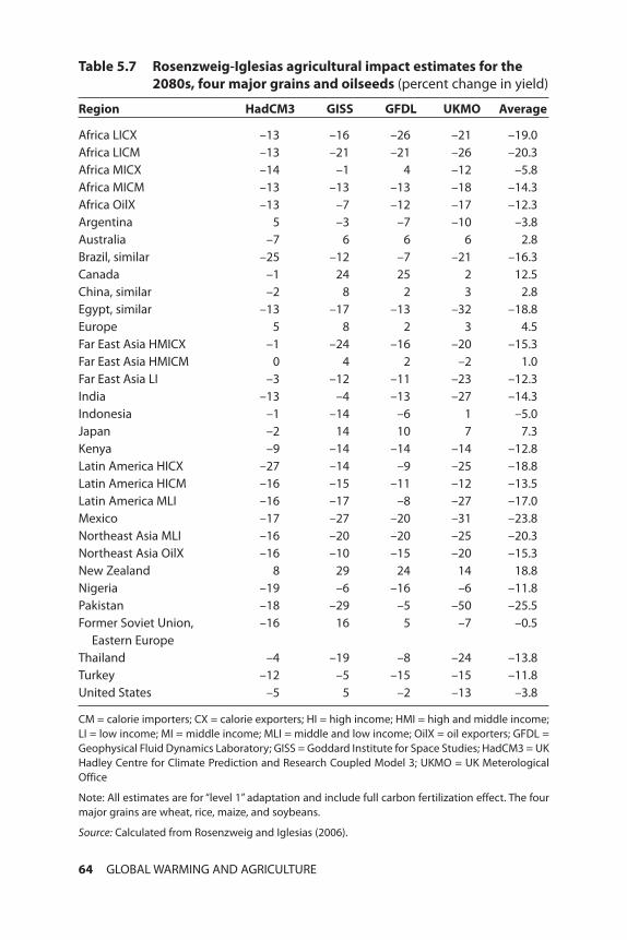
64 GLOBAL WARMING AND AGRICULTURE
Table 5.7 Rosenzweig-Iglesias agricultural impact estimates for the2080s, four major grains and oilseeds (percent change in yield)
Region HadCM3 GISS GFDL UKMO Average
Africa LICX –13 –16 –26 –21 –19.0Africa LICM –13 –21 –21 –26 –20.3Africa MICX –14 –1 4 –12 –5.8Africa MICM –13 –13 –13 –18 –14.3Africa OilX –13 –7 –12 –17 –12.3Argentina 5 –3 –7 –10 –3.8Australia –7 6 6 6 2.8Brazil, similar –25 –12 –7 –21 –16.3Canada –1 24 25 2 12.5China, similar –2 8 2 3 2.8Egypt, similar –13 –17 –13 –32 –18.8Europe 5 8 2 3 4.5Far East Asia HMICX –1 –24 –16 –20 –15.3Far East Asia HMICM 0 4 2 –2 1.0Far East Asia LI –3 –12 –11 –23 –12.3India –13 –4 –13 –27 –14.3Indonesia –1 –14 –6 1 –5.0Japan –2 14 10 7 7.3Kenya –9 –14 –14 –14 –12.8Latin America HICX –27 –14 –9 –25 –18.8Latin America HICM –16 –15 –11 –12 –13.5Latin America MLI –16 –17 –8 –27 –17.0Mexico –17 –27 –20 –31 –23.8Northeast Asia MLI –16 –20 –20 –25 –20.3Northeast Asia OilX –16 –10 –15 –20 –15.3New Zealand 8 29 24 14 18.8Nigeria –19 –6 –16 –6 –11.8Pakistan –18 –29 –5 –50 –25.5Former Soviet Union, –16 16 5 –7 –0.5
Eastern EuropeThailand –4 –19 –8 –24 –13.8Turkey –12 –5 –15 –15 –11.8United States –5 5 –2 –13 –3.8
CM = calorie importers; CX = calorie exporters; HI = high income; HMI = high and middle income;LI = low income; MI = middle income; MLI = middle and low income; OilX = oil exporters; GFDL =Geophysical Fluid Dynamics Laboratory; GISS = Goddard Institute for Space Studies; HadCM3 = UKHadley Centre for Climate Prediction and Research Coupled Model 3; UKMO = UK MeterologicalOffice
Note: All estimates are for “level 1” adaptation and include full carbon fertilization effect. The fourmajor grains are wheat, rice, maize, and soybeans.
Source: Calculated from Rosenzweig and Iglesias (2006).
01--Chs. 1-7--1-98 6/28/07 1:19 PM Page 64
in the same Ricardian family is the series of recent World Bank–supportedstudies on Latin America, with results of the models as applied here re-ported in table 5.5. The fourth source is for India, based on Mendelsohn,Dinar, and Sanghi (2001) and with results as applied here reported in table5.2. The fifth source is the Reinsborough (2003) study for Canada, whosefinding of zero impact of climate change is applied to both Canada and itslatitudinal peer Russia.
In the second framework, the estimates come from a different concep-tual approach, which uses crop models developed on the basis of agricul-tural science rather than statistical regressions across climate regions oflarge countries and which directly calculates the effects of reasonable lev-els of adaptation rather than assuming that cross-section regressions cap-ture adaptation. The Rosenzweig-Iglesias estimates provide the sole basisfor the crop model estimates for all countries except the United States. Forthe United States, the reduced form crop model function by Mendelsohnand Schlesinger (1999) is available as an alternative model synthesizingthis school, and its estimates (table 5.1) are given equal weight with theRosenzweig-Iglesias estimates for the United States.
The synthesis of preferred estimates then follows two alternative pro-cedures. For those countries for which the Ricardian estimates are avail-able from models specifically estimated for the country or region in ques-tion, the Ricardian estimates and the crop model estimates are given equalweight. This set of countries includes the United States, Canada, Africa,most of Latin America, and India. Russia is also treated in this fashion, forthe reasons discussed above. This first category of preferred estimates en-compasses about half of the total number of countries and 35 percent ofglobal agricultural production.
The second alternative approach applies to those countries without spe-cific regionally based Ricardian models, for which the default US model(MS cross-section, appendix table F.2) must be applied. Because of the po-tential misleading results when the US model is applied to other countries(as illustrated by the case of Canada), less weight is given to the Ricardianestimate than to the crop model estimate in these countries.23 For thesecountries, the weight is set at one-third for the default MS Ricardian esti-mates and two-thirds for the Rosenzweig-Iglesias crop model estimates.
These are the preferred estimates for the case with no carbon fertiliza-tion. The corresponding set of estimates including carbon fertilizationthen simply applies a 15 percent yield increase to the estimates without
COUNTRY-LEVEL AGRICULTURAL IMPACT ESTIMATES 65
23. As discussed above, the Reinsborough (2003) Ricardian model estimated directly forCanada shows virtually zero impact of future global warming on agricultural potential asproxied by farmland value. In contrast, the MS cross-section Ricardian model for the UnitedStates shows a remarkable doubling or more of Canadian agricultural potential from futureglobal warming (appendix table F.2).
01--Chs. 1-7--1-98 6/28/07 1:19 PM Page 65
carbon fertilization, based on the FACE studies as discussed above.24 Inpractice, the preferred estimates accept the underlying Mendelsohn-Schlesinger, Mendelsohn-Dinar-Sanghi, World Bank Africa, World BankLatin America, and Rosenzweig-Iglesias estimates for the non–carbon fer-tilization case but apply this study’s own preferred measure of the boostfrom carbon fertilization rather than accepting the corresponding esti-mates in the underlying studies.25
Table 5.8 reports the results of the preferred estimates. The table firstshows farm area, output per hectare, and corresponding total output foreach country or region for 2003. These output estimates serve as the basisfor weighting to obtain regional and global aggregates. Column D then re-ports the preferred framework 1 estimate in the Ricardian statistical modelfamily, as just discussed. Column E reports the source or basis for each ofthese estimates. Column F shows the crop model–based estimates. For allcountries but the United States, these are the Rosenzweig and Iglesias es-timates from table 5.7 converted to magnitudes excluding carbon fertiliza-tion (by removing a uniform 17.5 percent boost, the average for the fourclimate models in the Rosenzweig-Iglesias estimates). As noted, for theUnited States the crop model estimates are an average of these adjustedRosenzweig-Iglesias estimates and the MS reduced form estimates (fromappendix table F.1). Column G reports the geographical grouping that isthe source of the Rosenzweig-Iglesias estimate for the country in question.
Column H reports the preferred estimate for agricultural impact with-out carbon fertilization, following the procedure just discussed (equalweight for Ricardian and crop models where the regional or country Ri-cardian model is available—indicated as 1 in column I; one-third and two-thirds weight, respectively, where the general default Ricardian modelmust be used—indicated as 2 in column I). The corresponding preferredestimate including carbon fertilization is reported in column J. This esti-mate includes the effect of a uniform boost of 15 percent in yield from car-bon fertilization. These two respective percentage changes in agriculturalproductivity are then applied to each country’s base output to estimatethe implied absolute change in output potential, reported in columns Kand L. Aggregating these changes in potential output and comparing the
66 GLOBAL WARMING AND AGRICULTURE
24. With a uniform yield increase, the with–carbon fertilization estimates are a strict trans-formation of the without–carbon fertilization estimates because the expansion factors out ofthe detailed calculations regardless of the level of aggregation. Thus, with q as average out-put per hectare (for example), and with q = Σqi �i where �i is the weight applied to the dis-aggregated components of the aggregate in question, then the estimate q’ including carbonfertilization will uniformly be 1.15 x q, because Σ 1.15 qi �i = 1.15 Σqi �i. For its part, q ex-pressed as an index with value of 1 for base period productivity is simply q = 1 � d/100 forthe future period, where d is the estimate of the percent change in productivity from climatechange without including carbon fertilization.
25. Note that the World Bank–sponsored studies for Africa and Latin America do not esti-mate carbon fertilization effects.
01--Chs. 1-7--1-98 6/28/07 1:19 PM Page 66

67
Table 5.8 Preferred estimates of impact of baseline global warming by the 2080s on world agriculture
Impact without carbon fertilization Preferred estimates Change in output
Farm Output Without With(millions of 2003 dollars)
area (millionsRicardian Crop models
carbon carbon Without With(1,000 of 2003 Estimate Estimate fertilization fertilization carbon carbon
hectares) dollars) (percent) Basisa (percent) Groupingb (percent) Basisc (percent)d fertilization fertilizationCountry (A) (B) (C) (D) (E) (F) (G) (H) (I) (J) (K) (L)
Afghanistan 7,827 313 2,448 –9.5 1 –32.1 24 –24.7 2 –13.4 –604 –327Algeria 8,459 787 6,653 –46.7 2 –25.3 5 –36.0 1 –26.4 –2,394 –1,756Angola 3,300 360 1,187 –26.3 2 –25.3 5 –25.8 1 –14.7 –306 –174Argentina 172,106 83 14,256 –4.1 3 –18.1 6 –11.1 1 2.2 –1,581 320Australia 455,723 29 13,059 –55.1 1 –12.6 –26.6 2 –15.6 –3,471 –2,033
Southeast 192,824 16 3,147 –11.6 1 –12.6 7 –12.2 2 0.9 –385 29Southwest 84,778 14 1,212 –15.3 1 –12.6 7 –13.5 2 –0.5 –163 –6Central East 22,955 146 3,357 –45.5 1 –12.6 7 –23.4 2 –11.9 –787 –401Central West 84,838 14 1,213 –80.9 1 –12.6 7 –35.1 2 –25.4 –426 –308North 70,327 59 4,131 –100.0 1 –12.6 7 –41.4 2 –32.6 –1,711 –1,348
Bangladesh 8,429 1,355 11,421 –14.3 1 –25.3 15 –21.7 2 –9.9 –2,475 –1,133Belgium 1,428 2,114 3,019 2.2 1 –11.1 12 –6.7 2 7.3 –202 220Brazil 353,611 84 29,540 –5.1 3 –28.7 –16.9 1 –4.4 –4,976 –1,292
Amazon 41,593 29 1,215 –24.5 3 –28.7 8 –26.6 1 –15.6 –323 –190Northeast 95,062 48 4,574 –10.0 3 –28.7 8 –19.4 1 –7.3 –886 –332South 216,956 109 23,751 –3.0 3 –28.7 8 –15.9 1 –3.2 –3,767 –770
Burkina Faso 6,830 190 1,296 –16.5 2 –32.1 2 –24.3 1 –13.0 –315 –168Cambodia 3,807 378 1,438 –53.5 1 –14.0 14 –27.1 2 –16.1 –389 –232Cameroon 7,160 768 5,496 –20.3 2 –19.8 3 –20.0 1 –8.0 –1,100 –441Canada 67,504 254 17,146 0.0 5 –4.3 –2.2 1 12.5 –364 2,150
Arctic 0 0 0 0.0 5 –4.3 9 –2.1 1 12.6 0 0Central 44,401 254 11,268 0.0 5 –4.3 9 –2.1 1 12.6 –240 1,414Northwest Territories 0 0 0 0.0 5 –4.3 9 –2.1 1 12.6 0 0Pacific Coast 13,121 254 3,330 0.0 5 –4.3 9 –2.1 1 12.6 –71 418Southeast 9,980 254 2,533 0.0 5 –4.3 9 –2.1 1 12.6 –54 318
Output perhectare
(2003dollars)
(table continues next page)
01--Chs.
1-7--1-98
6/28/07
1:19
PM
Page
67
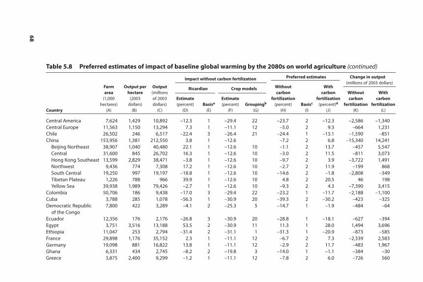
68
Central America 7,624 1,429 10,892 –12.3 1 –29.4 22 –23.7 2 –12.3 –2,586 –1,340Central Europe 11,563 1,150 13,294 7.3 1 –11.1 12 –5.0 2 9.3 –664 1,231Chile 26,502 246 6,517 –22.4 3 –26.4 21 –24.4 1 –13.1 –1,590 –851China 153,956 1,381 212,550 3.8 1 –12.6 –7.2 2 6.8 –15,340 14,241
Beijing Northeast 38,907 1,040 40,480 22.1 1 –12.6 10 –1.1 2 13.7 –457 5,547Central 31,600 845 26,702 16.3 1 –12.6 10 –3.0 2 11.5 –811 3,073Hong Kong Southeast 13,599 2,829 38,471 –3.8 1 –12.6 10 –9.7 2 3.9 –3,722 1,491Northwest 9,436 774 7,308 17.2 1 –12.6 10 –2.7 2 11.9 –199 868South Central 19,250 997 19,197 –18.8 1 –12.6 10 –14.6 2 –1.8 –2,808 –349Tibetan Plateau 1,226 788 966 39.9 1 –12.6 10 4.8 2 20.5 46 198Yellow Sea 39,938 1,989 79,426 –2.7 1 –12.6 10 –9.3 2 4.3 –7,390 3,415
Colombia 50,706 186 9,438 –17.0 3 –29.4 22 –23.2 1 –11.7 –2,188 –1,100Cuba 3,788 285 1,078 –56.3 1 –30.9 20 –39.3 2 –30.2 –423 –325Democratic Republic 7,800 422 3,289 –4.1 2 –25.3 5 –14.7 1 –1.9 –484 –64
of the CongoEcuador 12,356 176 2,176 –26.8 3 –30.9 20 –28.8 1 –18.1 –627 –394Egypt 3,751 3,516 13,188 53.5 2 –30.9 11 11.3 1 28.0 1,494 3,696Ethiopia 11,047 253 2,794 –31.4 2 –31.1 1 –31.3 1 –20.9 –873 –585France 29,898 1,176 35,152 2.3 1 –11.1 12 –6.7 2 7.3 –2,339 2,583Germany 19,098 881 16,822 13.8 1 –11.1 12 –2.9 2 11.7 –483 1,967Ghana 6,331 434 2,745 –8.2 2 –19.8 3 –14.0 1 –1.1 –384 –30Greece 3,875 2,400 9,299 –1.2 1 –11.1 12 –7.8 2 6.0 –726 560
Table 5.8 Preferred estimates of impact of baseline global warming by the 2080s on world agriculture (continued)
Impact without carbon fertilization Preferred estimates Change in output
Farm Output Without With(millions of 2003 dollars)
area (millionsRicardian Crop models
carbon carbon Without With(1,000 of 2003 Estimate Estimate fertilization fertilization carbon carbon
hectares) dollars) (percent) Basisa (percent) Groupingb (percent) Basisc (percent)d fertilization fertilizationCountry (A) (B) (C) (D) (E) (F) (G) (H) (I) (J) (K) (L)
Output perhectare
(2003dollars)
01--Chs.
1-7--1-98
6/28/07
1:19
PM
Page
68
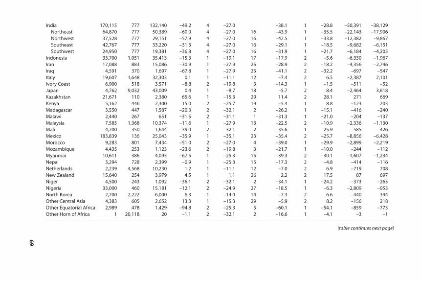
69
India 170,115 777 132,140 –49.2 4 –27.0 –38.1 1 –28.8 –50,391 –38,129Northeast 64,870 777 50,389 –60.9 4 –27.0 16 –43.9 1 –35.5 –22,143 –17,906Northwest 37,528 777 29,151 –57.9 4 –27.0 16 –42.5 1 –33.8 –12,382 –9,867Southeast 42,767 777 33,220 –31.3 4 –27.0 16 –29.1 1 –18.5 –9,682 –6,151Southwest 24,950 777 19,381 –36.8 4 –27.0 16 –31.9 1 –21.7 –6,184 –4,205
Indonesia 33,700 1,051 35,413 –15.3 1 –19.1 17 –17.9 2 –5.6 –6,330 –1,967Iran 17,088 883 15,086 –30.9 1 –27.9 25 –28.9 2 –18.2 –4,356 –2,746Iraq 4,591 370 1,697 –67.8 1 –27.9 25 –41.1 2 –32.2 –697 –547Italy 19,607 1,648 32,303 0.1 1 –11.1 12 –7.4 2 6.5 –2,387 2,101Ivory Coast 6,900 518 3,571 –8.8 2 –19.8 3 –14.3 1 –1.5 –511 –52Japan 4,762 9,032 43,009 0.4 1 –8.7 18 –5.7 2 8.4 –2,464 3,618Kazakhstan 21,671 110 2,380 65.6 1 –15.3 29 11.4 2 28.1 271 669Kenya 5,162 446 2,300 15.0 2 –25.7 19 –5.4 1 8.8 –123 203Madagascar 3,550 447 1,587 –20.3 2 –32.1 2 –26.2 1 –15.1 –416 –240Malawi 2,440 267 651 –31.5 2 –31.1 1 –31.3 1 –21.0 –204 –137Malaysia 7,585 1,368 10,374 –11.6 1 –27.9 13 –22.5 2 –10.9 –2,336 –1,130Mali 4,700 350 1,644 –39.0 2 –32.1 2 –35.6 1 –25.9 –585 –426Mexico 183,839 136 25,043 –35.9 1 –35.1 23 –35.4 2 –25.7 –8,856 –6,428Morocco 9,283 801 7,434 –51.0 2 –27.0 4 –39.0 1 –29.9 –2,899 –2,219Mozambique 4,435 253 1,123 –23.6 2 –19.8 3 –21.7 1 –10.0 –244 –112Myanmar 10,611 386 4,095 –67.5 1 –25.3 15 –39.3 2 –30.1 –1,607 –1,234Nepal 3,294 728 2,399 –0.9 1 –25.3 15 –17.3 2 –4.8 –414 –116Netherlands 2,239 4,568 10,230 1.2 1 –11.1 12 –7.0 2 6.9 –719 708New Zealand 15,640 254 3,979 4.5 1 1.1 26 2.2 2 17.5 87 697Niger 4,500 243 1,092 –36.1 2 –32.1 2 –34.1 1 –24.2 –373 –265Nigeria 33,000 460 15,181 –12.1 2 –24.9 27 –18.5 1 –6.3 –2,809 –953North Korea 2,700 2,222 6,000 6.3 1 –14.0 14 –7.3 2 6.6 –440 394Other Central Asia 4,383 605 2,652 13.3 1 –15.3 29 –5.9 2 8.2 –156 218Other Equatorial Africa 2,989 478 1,429 –94.8 2 –25.3 5 –60.1 1 –54.1 –859 –773Other Horn of Africa 1 20,118 20 –1.1 2 –32.1 2 –16.6 1 –4.1 –3 –1
(table continues next page)
01--Chs.
1-7--1-98
6/28/07
1:19
PM
Page
69
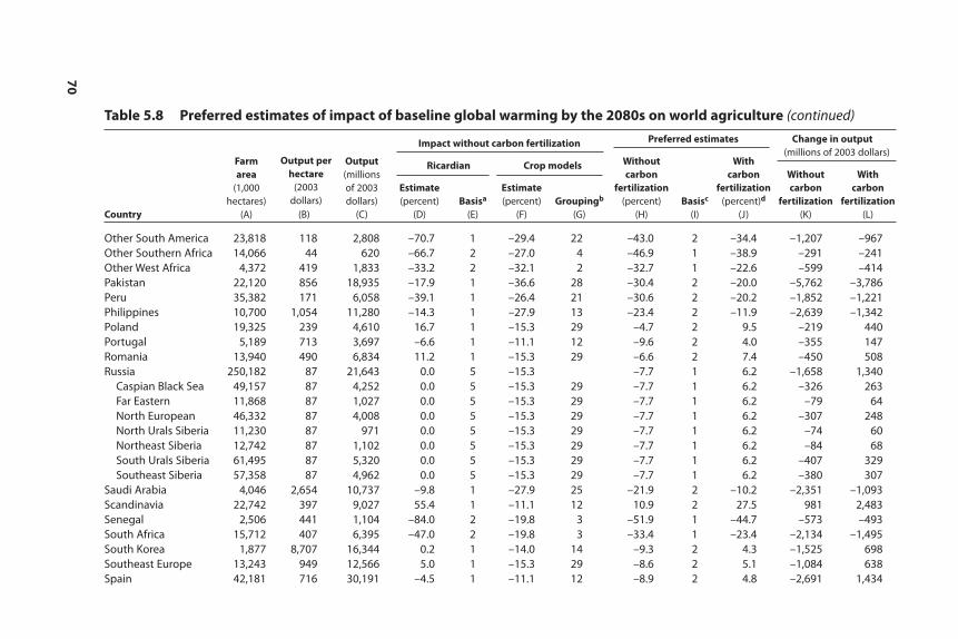
70
Other South America 23,818 118 2,808 –70.7 1 –29.4 22 –43.0 2 –34.4 –1,207 –967Other Southern Africa 14,066 44 620 –66.7 2 –27.0 4 –46.9 1 –38.9 –291 –241Other West Africa 4,372 419 1,833 –33.2 2 –32.1 2 –32.7 1 –22.6 –599 –414Pakistan 22,120 856 18,935 –17.9 1 –36.6 28 –30.4 2 –20.0 –5,762 –3,786Peru 35,382 171 6,058 –39.1 1 –26.4 21 –30.6 2 –20.2 –1,852 –1,221Philippines 10,700 1,054 11,280 –14.3 1 –27.9 13 –23.4 2 –11.9 –2,639 –1,342Poland 19,325 239 4,610 16.7 1 –15.3 29 –4.7 2 9.5 –219 440Portugal 5,189 713 3,697 –6.6 1 –11.1 12 –9.6 2 4.0 –355 147Romania 13,940 490 6,834 11.2 1 –15.3 29 –6.6 2 7.4 –450 508Russia 250,182 87 21,643 0.0 5 –15.3 –7.7 1 6.2 –1,658 1,340
Caspian Black Sea 49,157 87 4,252 0.0 5 –15.3 29 –7.7 1 6.2 –326 263Far Eastern 11,868 87 1,027 0.0 5 –15.3 29 –7.7 1 6.2 –79 64North European 46,332 87 4,008 0.0 5 –15.3 29 –7.7 1 6.2 –307 248North Urals Siberia 11,230 87 971 0.0 5 –15.3 29 –7.7 1 6.2 –74 60Northeast Siberia 12,742 87 1,102 0.0 5 –15.3 29 –7.7 1 6.2 –84 68South Urals Siberia 61,495 87 5,320 0.0 5 –15.3 29 –7.7 1 6.2 –407 329Southeast Siberia 57,358 87 4,962 0.0 5 –15.3 29 –7.7 1 6.2 –380 307
Saudi Arabia 4,046 2,654 10,737 –9.8 1 –27.9 25 –21.9 2 –10.2 –2,351 –1,093Scandinavia 22,742 397 9,027 55.4 1 –11.1 12 10.9 2 27.5 981 2,483Senegal 2,506 441 1,104 –84.0 2 –19.8 3 –51.9 1 –44.7 –573 –493South Africa 15,712 407 6,395 –47.0 2 –19.8 3 –33.4 1 –23.4 –2,134 –1,495South Korea 1,877 8,707 16,344 0.2 1 –14.0 14 –9.3 2 4.3 –1,525 698Southeast Europe 13,243 949 12,566 5.0 1 –15.3 29 –8.6 2 5.1 –1,084 638Spain 42,181 716 30,191 –4.5 1 –11.1 12 –8.9 2 4.8 –2,691 1,434
Table 5.8 Preferred estimates of impact of baseline global warming by the 2080s on world agriculture (continued)
Impact without carbon fertilization Preferred estimates Change in output
Farm Output Without With(millions of 2003 dollars)
area (millionsRicardian Crop models
carbon carbon Without With(1,000 of 2003 Estimate Estimate fertilization fertilization carbon carbon
hectares) dollars) (percent) Basisa (percent) Groupingb (percent) Basisc (percent)d fertilization fertilizationCountry (A) (B) (C) (D) (E) (F) (G) (H) (I) (J) (K) (L)
Output perhectare
(2003dollars)
01--Chs.
1-7--1-98
6/28/07
1:19
PM
Page
70
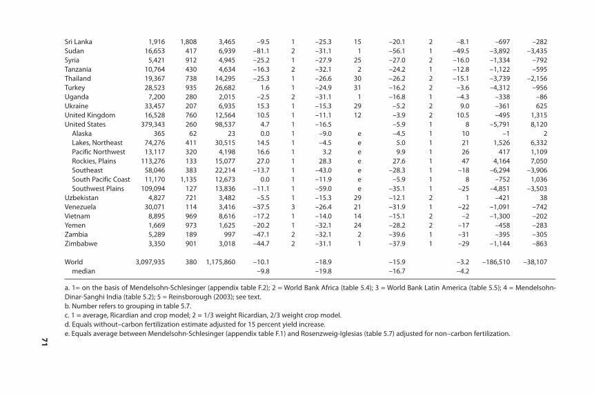
71
Sri Lanka 1,916 1,808 3,465 –9.5 1 –25.3 15 –20.1 2 –8.1 –697 –282Sudan 16,653 417 6,939 –81.1 2 –31.1 1 –56.1 1 –49.5 –3,892 –3,435Syria 5,421 912 4,945 –25.2 1 –27.9 25 –27.0 2 –16.0 –1,334 –792Tanzania 10,764 430 4,634 –16.3 2 –32.1 2 –24.2 1 –12.8 –1,122 –595Thailand 19,367 738 14,295 –25.3 1 –26.6 30 –26.2 2 –15.1 –3,739 –2,156Turkey 28,523 935 26,682 1.6 1 –24.9 31 –16.2 2 –3.6 –4,312 –956Uganda 7,200 280 2,015 –2.5 2 –31.1 1 –16.8 1 –4.3 –338 –86Ukraine 33,457 207 6,935 15.3 1 –15.3 29 –5.2 2 9.0 –361 625United Kingdom 16,528 760 12,564 10.5 1 –11.1 12 –3.9 2 10.5 –495 1,315United States 379,343 260 98,537 4.7 1 –16.5 –5.9 1 8 –5,791 8,120
Alaska 365 62 23 0.0 1 –9.0 e –4.5 1 10 –1 2Lakes, Northeast 74,276 411 30,515 14.5 1 –4.5 e 5.0 1 21 1,526 6,332Pacific Northwest 13,117 320 4,198 16.6 1 3.2 e 9.9 1 26 417 1,109Rockies, Plains 113,276 133 15,077 27.0 1 28.3 e 27.6 1 47 4,164 7,050Southeast 58,046 383 22,214 –13.7 1 –43.0 e –28.3 1 –18 –6,294 –3,906South Pacific Coast 11,170 1,135 12,673 0.0 1 –11.9 e –5.9 1 8 –752 1,036Southwest Plains 109,094 127 13,836 –11.1 1 –59.0 e –35.1 1 –25 –4,851 –3,503
Uzbekistan 4,827 721 3,482 –5.5 1 –15.3 29 –12.1 2 1 –421 38Venezuela 30,071 114 3,416 –37.5 3 –26.4 21 –31.9 1 –22 –1,091 –742Vietnam 8,895 969 8,616 –17.2 1 –14.0 14 –15.1 2 –2 –1,300 –202Yemen 1,669 973 1,625 –20.2 1 –32.1 24 –28.2 2 –17 –458 –283Zambia 5,289 189 997 –47.1 2 –32.1 2 –39.6 1 –31 –395 –305Zimbabwe 3,350 901 3,018 –44.7 2 –31.1 1 –37.9 1 –29 –1,144 –863
World 3,097,935 380 1,175,860 –10.1 –18.9 –15.9 –3.2 –186,510 –38,107median –9.8 –19.8 –16.7 –4.2
a. 1= on the basis of Mendelsohn-Schlesinger (appendix table F.2); 2 = World Bank Africa (table 5.4); 3 = World Bank Latin America (table 5.5); 4 = Mendelsohn-Dinar-Sanghi India (table 5.2); 5 = Reinsborough (2003); see text.b. Number refers to grouping in table 5.7.c. 1 = average, Ricardian and crop model; 2 = 1/3 weight Ricardian, 2/3 weight crop model.d. Equals without–carbon fertilization estimate adjusted for 15 percent yield increase.e. Equals average between Mendelsohn-Schlesinger (appendix table F.1) and Rosenzweig-Iglesias (table 5.7) adjusted for non–carbon fertilization.
01--Chs.
1-7--1-98
6/28/07
1:19
PM
Page
71

results with aggregated base output provides the basis for obtaining thepercent change in agricultural potential at the global (table 5.8) and re-gional levels (discussed later). As discussed in chapter 3, these output ef-fects represent direct supply impact before taking into account inducedeffects from price changes and from adjustments in international trade.
The global result in the preferred estimates is that business as usual cli-mate change by the 2080s would reduce world agricultural production ca-pacity by about 16 percent if carbon fertilization is omitted and by about3 percent if it is included. A 16 percent reduction would be severe andwould potentially cause major price increases because of the inelasticityof demand for food. These price increases would need to be taken into ac-count in estimating resulting global welfare losses.
Even if the moderate global reduction of 3 percent assuming carbon fer-tilization were the outcome, the large disparity of results across countrieswould mean much more serious losses for many countries and regions.Generally, the developing countries would tend to fare much worse thanthe industrial countries, as examined later.
There are 21 countries, regions, or subzones of large countries in whichproduction capacity falls by more than one-third without carbon fertiliza-tion and 7 in which it does so even with carbon fertilization. If the thresh-old is set at a loss of 20 percent or greater, there are 53 countries and re-gions with severe losses without carbon fertilization and 29 even withcarbon fertilization.
For the United States, there would be moderate results overall but sharpdisparities among regions. Without carbon fertilization, there would be aloss of 5.9 percent for the United States, but this outcome masks dispersionbetween gains as high as 28 percent in the Rockies and Plains and lossesin the range of 30 percent in the Southeast and Southwest Plains.26 For theUS results including carbon fertilization, the corresponding estimates arean overall average gain of 8 percent, with impacts as favorable as �47 per-cent in the Rockies and Plains but as unfavorable as –18 percent in theSoutheast and –25 percent in the Southwest Plains.
India would face a major loss on the order of 30 percent even with car-bon fertilization. The loss would be about 35 percent in the Northeast andNorthwest. In the key case of China, the aggregate gains would be about7 percent assuming carbon fertilization but losses of 7 percent if carbonfertilization failed to materialize. Moreover, in the case without carbonfertilization, losses would be as high as 15 percent in the South Central re-gion, which accounts for about 140 million people (appendix E and ERS2006a).
72 GLOBAL WARMING AND AGRICULTURE
26. The Rockies-Plains gains are probably overstated, moreover, by using land area ratherthan output value to aggregate from the standard grid level up to the region. This wouldtend to give substantial weight to supposed gains from warming in the cold mountainousareas even though their topography constrains agricultural potential.
01--Chs. 1-7--1-98 6/28/07 1:19 PM Page 72
Figures 5.2 and 5.3 portray the preferred results graphically. The sub-stantially more favorable results when carbon fertilization is included(figure 5.3) are evident in most regions. These maps also underscore theconcentration of damage in the latitudes closer to the equator and of gainsin latitudes closer to the poles. With the exception of New Zealand, theSouthern Hemisphere is nearly uniform in experiencing losses, reflectingthe paucity of land masses in the latitudes south of about 35°S. Losses are also predominant in the Northern Hemisphere below about 35°N, but a much smaller fraction of total land area lies between the equator and35°N than in the corresponding zone in the Southern Hemisphere.
The underlying components shown in table 5.8 for the preferred esti-mates provide a basis for a broad comparison between results from the Ri-cardian family and those from the crop model family. As discussed above,only those countries or regions with specific Ricardian function estimatesare given full equal weight to the crop model estimates, so it is most use-ful to limit the comparison to these countries and regions (indicated by 1 for the basis for the preferred estimates in column I of table 5.8).
Figure 5.4 plots the percent change in agricultural potential (withoutcarbon fertilization) for the 47 regions for which a regionally or country-specific Ricardian estimate exists, showing the Ricardian estimate on thevertical axis and the crop model (Rosenzweig-Iglesias for all but theUnited States) estimate on the horizontal axis. The scale of the two axes im-mediately confirms one major pattern: The crop model results show con-siderably less dispersion than the Ricardian results. The wider dispersionof the Ricardian estimates is confirmed by their standard deviation, whichis 28 percentage points versus 12.1 percent for the crop model estimates.One underlying reason seems to be that the Rosenzweig-Iglesias cropmodel findings tend to be linear with regard to the magnitude of climatechange, whereas at least the models in the Ricardian family are nonlinear.27
The pattern of the scatter diagram indicates that there is a reasonabledegree of agreement between the two sets.28 Given the figure scale, com-plete agreement would place all observations along the 17.5° line. Theagreement is far from complete. Nonetheless there is a clear upward slopein the scatter, meaning that high estimates in one set are also high in theother, and the large negative estimates in one set also tend to be large neg-ative estimates in the other. The two sets of estimates yield comparable
COUNTRY-LEVEL AGRICULTURAL IMPACT ESTIMATES 73
27. Thus, Parry, Rosenzweig, and Livermore (2005, 2136) state that: “Without the counter-acting direct CO2 effects, crop production responds approximately linearly to temperatureincreases across the suite of scenarios.”
28. The simple correlation coefficient between the two sets of estimates is 0.38. A regressionof the Ricardian estimates on the crop model estimates yields a statistically significant coef-ficient of 0.73 (t-statistic of 2.3). Note that the observation of greatest disagreement is that forEgypt, with 53 percent gain in the Ricardian estimate but 31 percent loss in the crop modelestimates.
01--Chs. 1-7--1-98 6/28/07 1:19 PM Page 73
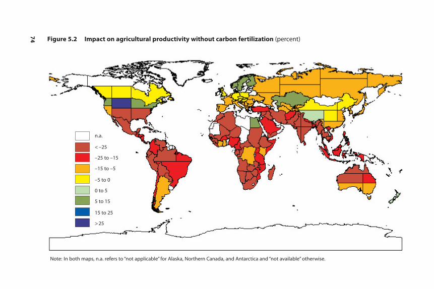
74 Figure 5.2 Impact on agricultural productivity without carbon fertilization (percent)
n.a.
< –25
–25 to –15
–15 to –5
–5 to 0
0 to 5
5 to 15
15 to 25
>25
Note: In both maps, n.a. refers to “not applicable” for Alaska, Northern Canada, and Antarctica and “not available” otherwise.
01--Chs.
1-7--1-98
6/28/07
1:19
PM
Page
74
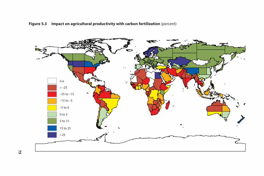
75
Figure 5.3 Impact on agricultural productivity with carbon fertilization (percent)
n.a.
< –25
–25 to –15
–15 to –5
–5 to 0
0 to 5
5 to 15
15 to 25
>25
01--Chs.
1-7--1-98
6/28/07
1:19
PM
Page
75
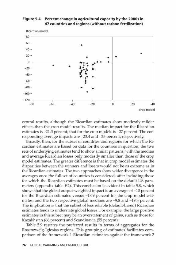
central results, although the Ricardian estimates show modestly mildereffects than the crop model results. The median impact for the Ricardianestimates is –21.3 percent; that for the crop models is –27 percent. The cor-responding average impacts are –23.4 and –25 percent, respectively.
Broadly, then, for the subset of countries and regions for which the Ri-cardian estimates are based on data for the countries in question, the twosets of underlying estimates tend to show similar patterns, with the medianand average Ricardian losses only modestly smaller than those of the cropmodel estimates. The greater difference is that in crop model estimates thedisparities between the winners and losers would not be as extreme as inthe Ricardian estimates. The two approaches show wider divergence in theaverages once the full set of countries is considered, after including thosefor which the Ricardian estimates must be based on the default US para-meters (appendix table F.2). This conclusion is evident in table 5.8, whichshows that the global output-weighted impact is an average of –10 percentfor the Ricardian estimates versus –18.9 percent for the crop model esti-mates, and the two respective global medians are –9.8 and –19.8 percent.The implication is that the subset of less reliable (default-based) Ricardianestimates tends to understate global losses. For example, the large positiveestimates in this subset may be an overstatement of gains, such as those forKazakhstan (66 percent) and Scandinavia (55 percent).
Table 5.9 restates the preferred results in terms of aggregates for theRosenzweig-Iglesias regions. This grouping of estimates facilitates com-parison of the framework 1 Ricardian estimates against the framework 2
76 GLOBAL WARMING AND AGRICULTURE
Figure 5.4 Percent change in agricultural capacity by the 2080s in 47 countries and regions (without carbon fertilization)
–120
–100
–80
–60
–40
–20
0
20
40
60
80
Ricardian model
crop model
–80 –60 –40 –20 40200
01--Chs. 1-7--1-98 6/28/07 1:19 PM Page 76

COUNTRY-LEVEL AGRICULTURAL IMPACT ESTIMATES 77
Table 5.9 Change in agricultural capacity by regional aggregates (percent)
Without carbon fertilization With carbon fertilizationa
Crop CropRegionb Ricardian model Preferred Ricardian model Preferred
Africa LICX –52.6 –31.1 –41.8 –45.5 –20.7 –33.1Africa LICM –26.1 –32.1 –29.1 –15.0 –21.9 –18.4Africa MICX –28.3 –19.8 –24.2 –17.5 –7.8 –12.8Africa MICM –52.2 –27.0 –39.6 –45.0 –16.1 –30.5Africa OilX –28.4 –25.3 –32.2 –17.7 –14.1 –22.0Argentina –4.1 –18.1 –11.1 10.3 –5.8 2.2Australia –55.1 –12.6 –26.6 –48.3 0.6 –15.6Brazil, similar –5.0 –28.7 –16.8 9.3 –18.0 –4.4Canada 0.0 –4.3 –2.1 15.0 10.1 12.6China, similar 3.6 –12.6 –7.2 19.2 0.6 6.7Egypt, similar 53.5 –30.9 11.3 76.5 –20.5 28.0Europe 5.1 –11.1 –5.7 20.8 2.3 8.4Far East Asia HMICX –13.0 –27.9 –23.0 0.0 –17.1 –11.4Far East Asia HMICM –5.7 –14.0 –11.3 8.5 –1.1 2.0Far East Asia LI –22.2 –25.3 –24.3 –10.5 –14.1 –12.9India –49.2 –27.0 –38.1 –41.6 –16.1 –28.9Indonesia –15.3 –19.1 –17.9 –2.6 –7.0 –5.6Japan 0.4 –8.7 –5.7 15.4 5.0 8.4Kenya 15.0 –25.7 –5.4 32.3 –14.6 8.8Latin America HICX –36.6 –30.9 –32.3 –27.0 –20.5 –22.1Latin America HICM –31.9 –26.4 –28.3 –21.7 –15.3 –17.6Latin America MLI –21.3 –29.4 –25.8 –9.5 –18.8 –14.7Mexico –35.9 –35.1 –35.4 –26.3 –25.4 –25.7Northeast Asia MLI –13.8 –32.1 –26.1 –0.9 –21.9 –15.0Northeast Asia OilX –25.0 –27.9 –26.9 –13.7 –17.1 –15.9New Zealand 4.5 1.1 2.2 20.2 16.2 17.5Nigeria –12.1 –24.9 –18.5 1.1 –13.6 –6.3Pakistan –17.9 –36.6 –30.4 –5.6 –27.1 –20.0Former Soviet Union, 8.1 –15.3 –6.7 24.3 –2.6 7.3
Eastern EuropeThailand –25.3 –26.6 –26.2 –14.1 –15.6 –15.1Turkey 1.6 –24.9 –16.2 16.8 –13.6 –3.6United States 4.7 –16.5 –5.9 20.4 –3.9 8.2
WorldMedian of regions –14.5 –25.5 –23.6 –1.7 –14.4 –12.1Total –10.0 –18.9 –15.9 3.5 –6.8 –3.2
Developing countriesMedian of regions –21.3 –27.0 –25.8 –9.5 –16.1 –14.7Total –16.9 –22.5 –21.0 –4.5 –10.8 –9.2
Industrial countriesMedian of regions 2.4 –9.9 –5.7 17.8 3.6 8.4Total 1.9 –11.9 –6.3 17.2 1.3 7.8
Economies in transition 8.1 –15.3 –6.7 24.3 –2.6 7.3(former Soviet Union, Eastern Europe)
a. Equals without carbon fertilization result plus effect of uniform 15 percent yield increase.b. See table 5.7.
Source: Table 5.8.
01--Chs. 1-7--1-98 6/28/07 1:19 PM Page 77
crop model estimates. The table shows them individually along with thepreferred regional estimates.
Several important findings are evident in table 5.9. First, at the globallevel and weighting by base output, the two sets of underlying estimatesonce again tend to show more severe effects in the crop model estimatesthan in the Ricardian estimates. In the case without carbon fertilization,global output capacity would fall by about 10 percent in the Ricardianmodel–based estimates and about 19 percent in the crop model estimates(the same as in table 5.8). The corresponding median changes show asomewhat wider divergence as well as larger damages for both, at about–15 and –26 percent, respectively. In the results including carbon fertiliza-tion, the differences persist, with a global average gain of 4 percent for theRicardian models but a loss of 7 percent for the crop model estimates andcorresponding median impacts across the various regions at –2 and –14percent, respectively.
Second, once again there is less dispersion between severe negative ef-fects and large positive effects in the crop model results than in the Ricar-dian results. In the groupings of table 5.9 the simple average impact forthe worst quintile (6 groupings) is –44 percent for the Ricardian estimates(without carbon fertilization) versus –33 percent for the crop model esti-mates. Conversely, the most favorable quintile of results shows an aver-age of �15 percent for the Ricardian estimates but –8 percent for the cropmodel estimates.
Third, in both sets of results most countries and regions would experi-ence larger losses than would be seen if attention focused solely on globalaggregates, as indicated by the differences between the average and me-dian estimates already noted. For the 32 regions, in the Ricardian-based es-timates the median losses are about 50 percent larger than the global aver-age in the case without carbon fertilization. With carbon fertilization thereare losses for the median region (1.7 percent) but a slight gain for the globalaggregate (3.5 percent). The median losses are also higher than the globalaverages in the crop model estimates but to a lesser degree (multiples of1.35 and 2 for the without and with carbon fertilization cases, respectively),reflecting the previous point about dispersion of results in the two sources.
Fourth, and in this same vein, both sets of estimates confirm that de-veloping countries would fare substantially worse than industrial coun-tries. In the case including carbon fertilization, for developing countriesthe median change in productive potential is a decline of about 16 (cropmodel) to 10 percent (Ricardian). In contrast, for industrial countries, thecorresponding medians show an increase of about 4 (crop model) to 18percent (Ricardian).
Finally, the detailed preferred results of table 5.8 can be aggregated intoan alternative grouping of developing and industrial countries based onmore usual geographical regions than in the Rosenzweig-Iglesias analysisin order to consider further the differences in impact between the two sets
78 GLOBAL WARMING AND AGRICULTURE
01--Chs. 1-7--1-98 6/28/07 1:19 PM Page 78
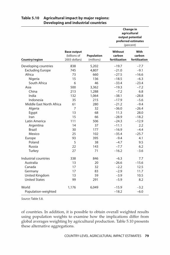
of countries. In addition, it is possible to obtain overall weighted resultsusing population weights to examine how the implications differ fromglobal averages weighting by agricultural production. Table 5.10 presentsthese alternative aggregations.
COUNTRY-LEVEL AGRICULTURAL IMPACT ESTIMATES 79
Table 5.10 Agricultural impact by major regions:Developing and industrial countries
Change in agricultural
output potentialpreferred estimates
(percent)
Base output Without With(billions of Population carbon carbon
Country/region 2003 dollars) (millions) fertilization fertilization
Developing countries 838 5,202 –19.7 –7.7Excluding Europe 745 4,807 –21.0 –9.1Africa 73 660 –27.5 –16.6
Nigeria 15 136 –18.5 –6.3South Africa 6 46 –33.4 –23.4
Asia 500 3,362 –19.3 –7.2China 213 1,288 –7.2 6.8India 132 1,064 –38.1 –28.8Indonesia 35 215 –17.9 –5.6
Middle East North Africa 61 280 –21.2 –9.4Algeria 7 32 –36.0 –26.4Egypt 13 68 11.3 28.0Iran 15 66 –28.9 –18.2
Latin America 111 506 –24.3 –12.9Argentina 14 37 –11.1 2.2Brazil 30 177 –16.9 –4.4Mexico 25 102 –35.4 –25.7
Europe 93 395 –9.4 4.1Poland 5 38 –4.7 9.5Russia 22 143 –7.7 6.2Turkey 27 71 –16.2 –3.6
Industrial countries 338 846 –6.3 7.7Australia 13 20 –26.6 –15.6Canada 17 32 –2.2 12.5Germany 17 83 –2.9 11.7United Kingdom 13 59 –3.9 10.5United States 99 291 –5.9 8.2
World 1,176 6,049 –15.9 –3.2Population-weighted –18.2 –6.0
Source: Table 5.8.
01--Chs. 1-7--1-98 6/28/07 1:19 PM Page 79
At the most aggregate level, the comparison between narrowly defineddeveloping countries and industrial countries is the same in tables 5.9 and5.10. Namely, including carbon fertilization, output-weighted agriculturalpotential rises for industrial countries by a preferred estimate of 7.7 per-cent, whereas for developing countries defined as excluding developingEurope it falls by 9.1 percent. The additional regional information in table5.10 shows that in the preferred estimate (and including carbon fertiliza-tion), output potential falls by about 17 percent in Africa excluding NorthAfrica, by 7 percent in Asia, 9 percent in the Middle East and North Africa,and 13 percent in Latin America. In contrast, for developing Europe it risesby 4 percent, the same broad range as the 7 percent in table 5.9 for the for-mer Soviet Union and Eastern Europe.29
These results indicate that Africa (excluding Egypt and other NorthAfrica) and Latin America are the two developing regions most vulnera-ble to global warming. This finding is consistent with the IPCC (1996) pat-tern noted in the survey above. Asia on average is less vulnerable, but thismasks the divergence between more favorable results for China in partic-ular and more unfavorable results for India, reflecting in part the differ-ence in their latitudes.
At the world level the aggregates are again the same as in tables 5.8 and5.9. Weighting by output, global agricultural potential falls by about 16percent without carbon fertilization and 3 percent with carbon fertiliza-tion. Table 5.10 also reports the global impact weighting by populationrather than output. In this case, output potential falls by a weighted aver-age of 18 percent without carbon fertilization and by about 6 percent withcarbon fertilization. The greater decline in output potential weighting bypopulation reflects the predominance of more severe adverse effects indeveloping countries in contrast to milder losses or even gains in indus-trial countries.
Comparison to Estimates in the Model-Source Studies
The analysis above has applied models developed by other authors to de-tailed future climate data as calculated in this study to obtain estimates of the impact of global warming on agricultural potential. The authors ofthese models have in some cases provided their own estimates of globalwarming impact, so it is important to compare their results with those here.
80 GLOBAL WARMING AND AGRICULTURE
29. Developing Europe in table 6.1 shares Russia, Poland, Romania, Southeastern Europe,and Ukraine with former Soviet Union and Eastern Europe in table 5.10. It adds Turkey andCentral Europe but drops Kazakhstan, Uzbekistan, and other Central Asia, which are real-located to Asia.
01--Chs. 1-7--1-98 6/28/07 1:19 PM Page 80
Mendelsohn, Morrison, Schlesinger, and Andronova
The Mendelsohn and Schlesinger (1999) models used in appendix tablesF.1 and F.2 were not used by their authors to calculate the impact of globalwarming on world agriculture, but a subsequent study by Mendelsohn,Morrison, Schlesinger, and Andronova (MMSA; 2000) made such esti-mates. The models in MMSA are almost identical to the reduced form andcross-section models in Mendelsohn and Schlesinger (1999). The only sub-stantial difference is that in the cross-section model the MMSA coefficientfor carbon fertilization is 43 percent larger than the corresponding coeffi-cient in the MS version (equation 5.2 above). With the benefit of hindsightin view of the recent FACE agronomic results, this increase appears tohave been ill-advised.
Applying their models, MMSA arrive at a very benign prognosis of theimpact of global warming by 2100 for the world as a whole.30 They state:
The aggregate impacts are projected to be beneficial in every scenario relative tothe current climate and carbon dioxide levels. . . . With the Ricardian model, ben-efits climb for the first 2°C of warming and then they decline. . . . With the re-duced-form model, warming benefits climb through 1°C and then just begin to de-cline at 2°C. Warming begins to be harmful between 1 and 2°C. The overallmagnitude of the market impacts [including forestry, coastal resources, energy,and water] is small in all cases, being less than 0.16% of world GDP. Thus, theseinitial results imply that global warming over the next century is not a seriousthreat to the world economy, and is likely to be a small benefit (Mendelsohn, Mor-rison, Schlesinger, and Andronova 2000, 560).
MMSA find small global net losses in the other market sectors they in-clude, and their conclusion just cited is entirely attributable to their esti-mate that there would be global gains from agriculture, amounting to$297 billion at 1990 prices in the cross-section model and $171 billion inthe reduced form model, against a global economy of $172 trillion by 2100in the central case. Chapter 6 of this study suggests that by 2085 globalagricultural demand is likely to expand by a multiple in the range of 2.7to 3.7 times the 2005 level. With world agricultural output at about $1.2trillion in 2003 (appendix E), by 2085 world agricultural output would beon the order of $3.8 trillion. The potential gain from global warming ofabout $300 billion estimated by MMSA in their Ricardian model would
COUNTRY-LEVEL AGRICULTURAL IMPACT ESTIMATES 81
30. It should be noted that nowhere in their study do MMSA report the paradox encoun-tered in the present study when applying both the reduced form and cross-section models:A high incidence of negative base period agricultural productivity is calculated when theseUS-based models are applied to the temperature and precipitation averages for other coun-tries. Correspondingly, they do not report how they address this problem or whether theyuse the approach applied here of considering the change in output per hectare from climatechange against an estimate of base period actual productivity, even where the predicted baselevel is negative.
01--Chs. 1-7--1-98 6/28/07 1:19 PM Page 81

thus represent a favorable impact of 8 percent of world agricultural out-put potential.
The results in the present study using the same underlying MS modelsare much less favorable (appendix tables F.1 and F.2). Thus, even includ-ing the MS carbon fertilization estimates, their reduced form model is es-timated here to generate a global loss of 13 percent in agricultural poten-tial, rather than a sizable gain. One key source of the difference is that theclimate model MMSA use (University of Illinois) generates 2°C meanglobal warming by 2100, whereas the suite of climate models used for thepresent study places mean global warming at 3°C by the 2080s. Becausetheir models find improvement at up to 1 to 2°C warming, it is no coinci-dence that using 2°C mean warming does not show damage and in factshows small gains.31 The other likely source of the difference in aggregateresults is from carbon fertilization. The MMSA version of the cross-sectionmodel would appear to overstate the carbon fertilization effect. Whenapplied to the 2080s climate, the MMSA carbon fertilization parameterboosts land rental equivalent by 46 percent above levels it would other-wise have reached, which globally would correspond to an increase inoutput potential by about half as much or 23 percent, well above the 15percent adopted in the present study (see chapter 3). In short, the basicsources of the difference between the benign global effects in MMSA andthe more adverse ones in the present study using the same basic modelswould seem to be the use of lower expected future warming and highercarbon fertilization in the MMSA study than in the present study.32
In contrast to the divergence in global aggregate estimates, for the pat-tern of regional and country winners and losers there is more similaritybetween the results here in appendix F using the MS models and those inMMSA. Both identify Canada and Russia as large beneficiaries (MMSAplace Russia’s agricultural gains at $124 billion to $351 billion at 1990prices and Canada’s gains at $19 billion to $49 billion). This same patternof large gains in Canada and Russia is found for the MS reduced form andRicardian estimates shown in appendix F, but as noted above, for themain estimates of this study the zero impact findings of Reinsborough(2003) are instead applied, for both countries. The strong MMSA gains for
82 GLOBAL WARMING AND AGRICULTURE
31. Although it is not quite that simple: As discussed above, the relevant warming over landareas significantly exceeds the global mean, so the land areas even in MMSA should showwarming higher than 2°C.
32. It is also possible that the coarser grid specification in the MMSA climate model thanthat in this study contributes to the difference. With grids of 4º latitude and 5º longitude, in-stead of 2º latitude and 3º longitude used in this study, their grid areas are 3.2 times as largeas those in this study. Even so, simple back-of-the-envelope application of the functions inequations (5.1) and (5.2) to the much more aggregative country climate averages shown intable 4.2 generates results broadly similar to the detailed results of this study built up fromthe grid level, so grid size seems unlikely to account for much of the difference between theMMSA results and those in this study.
01--Chs. 1-7--1-98 6/28/07 1:19 PM Page 82
China ($39 billion to $65 billion) and the United States ($17 billion to $35billion) are in the same direction, although larger, than the results fromapplication of the MS models in appendix F of the present study.
For developing countries, the MMSA results generally parallel thosefound here. In the reduced form model, India and Brazil both experiencelarge losses (by $86 billion and $106 billion annually, respectively). The re-duced form model in MMSA gives severe losses for Africa ($131 billion)and Latin America as a whole ($49 billion). However, the Ricardian (cross-section) model in MMSA shows gains even for these two regions, in con-trast to the results here. The MMSA finding of positive results for the cross-section function in all regions is in sharp contradiction to the cross-sectionfindings in the present study in appendix table F.2. This divergence mayin particular reflect the much stronger carbon fertilization effect used inMMSA than in the estimates here. Overall, nonetheless, it is fair to say thatthere is much more agreement between the MMSA findings and thosehere, especially using the reduced form rather than Ricardian cross-sectionmodel, on the differential effects among countries (including the broadpattern of losses in Africa and Latin America, in particular, in contrast tomore favorable results in industrial countries) than on the severity of thelosses and the overall global balance of results.
Mendelsohn, Dinar, and Sanghi
The model used for India is from Mendelsohn, Dinar, and Sanghi (2001).In that study, however, the authors focus on how the level of developmentaffects the climate sensitivity of agriculture. They do not include specificcalculations of the impact of prospective global warming on agriculture.
An earlier study by the same authors does provide impact estimates forIndia. Sanghi, Mendelsohn, and Dinar (1998, 107) develop a Ricardianmodel for Indian agriculture and calculate that benchmark global warm-ing (2 � CO2) would reduce net revenue by 12.3 percent. However, theircalculation applies 2°C rise in temperature and 7 percent rise in precipita-tion for benchmark climate change. Instead, it is evident from table 4.2that the consensus estimate from the six climate models considered in thepresent study would place climate change by the 2080s at much greaterwarming—a rise of 3.6°C for annual average temperature across the foursubzones. Although the corresponding estimate in the present study forprecipitation is also higher (at 17 rather than 7 percent), in the model inquestion the favorable impact of higher precipitation is much smaller thanthe unfavorable impact of higher temperatures.33 One reason the authors
COUNTRY-LEVEL AGRICULTURAL IMPACT ESTIMATES 83
33. The 7 percent boost in precipitation raises average net revenue by 14.4 rupees perhectare (at 1980 prices) whereas the 2°C increase in temperature reduces net revenue by 208rupees per hectare (Sanghi, Mendelsohn, and Dinar 1998, 98).
01--Chs. 1-7--1-98 6/28/07 1:19 PM Page 83
apply much less warming than used in the present study may be that theyhave implicitly assumed the change for India is the same as the global av-erage, whereas the increase for land areas would tend to be greater thanthe global average including the oceans (as emphasized above).
World Bank Studies
Africa. In the recent World Bank study on Africa (Kurukulasuriya et al.2006), the authors do not apply their models to a postulated future climatewith global warming, so once again there is no basis for direct compari-son with the results of the present study. Qualitatively, however, the studyappears to conclude that global warming has a neutral effect on Africa be-cause gains for irrigated agriculture approximately offset losses in dry-land agriculture. In particular, they find that for a 1°C temperature in-crease, the models calculate a “slight and insignificant increase [emphasisadded] in net revenue across African farms . . .” (p. 13).
The use of 1°C warming as the gauge makes this finding essentially ir-relevant to the question of effects by the end of this century. In particular,by the 2080s the simple average rise in annual average temperature for theAfrican countries and regions shown in table 4.2 is 4°C. Even within theconfines of the minimal 1°C warming, the result is misleading because itdepends on applying the with-Egypt function for irrigated farming. Asdiscussed above, the without-Egypt function shows a negative ratherthan positive response to warming, and Egypt’s atypical access to the NileRiver (and its atypical 100 percent irrigated farming in contrast to onlyabout 6 percent for Africa as a whole) would surely counsel use of thewithout-Egypt function to assess the impact on irrigated agriculture out-side Egypt, as is done here.
Perhaps more fundamentally, the “irrigation compensation” message inthe World Bank study does not come to grips with the problem that lesswater may be available for irrigation in a hotter and drier future. Thus,IPCC (2001b, 289) finds that
Africa is the continent with the lowest conversion factor of precipitation to run-off . . . . Although the equatorial region and coastal areas of eastern and southernAfrican are humid, the rest of the continent is dry subhumid to arid. The domi-nant impact of global warming is predicted to be a reduction in soil moisture insubhumid zones and reduction in runoff.
Indeed, the question of water availability for future irrigation poses aproblem for the applicability of the Ricardian models that do not evaluateirrigated agriculture separately (the MS cross-section model in particular),because one of the prime reasons farms can adjust in hotter and drier cli-mates is through increased irrigation. To the extent that the US-based MSfunction implicitly relies on greater irrigation as the vehicle for benign ef-
84 GLOBAL WARMING AND AGRICULTURE
01--Chs. 1-7--1-98 6/28/07 1:19 PM Page 84
fects of warming, it will give an unduly optimistic picture of future agri-cultural prospects in those areas where irrigation would be increasinglyconstrained because of adverse effects on water availability.
In a related study using the World Bank Africa surveys, Kurukulasuriyaand Mendelsohn (2006) apply alternative climate models to each country.They find that by the end of this century, and excluding carbon fertiliza-tion, Africa as a whole could experience agricultural impacts rangingfrom annual losses of $48 billion if the future climate were “hot and dry”to annual gains of $97 billion if it were “mild and wet” (p. 7). The effectsare not uniform across countries, and the hotter and drier regions ofAfrica fare the worst in all scenarios. The African estimates in the presentstudy suggest, however, that this wide range, and especially its average of�$25 billion, are likely to be misleading and that instead the best guessusing a consensus climate model is that large losses would predominate.
Latin America. The discussion above of the recent World Bank–sponsoredstudies for Latin America, and the estimates presented in table 5.5, di-rectly address the climate impact estimates contained in that set of stud-ies in comparison with the corresponding results obtained using theirmodels with the climate assumptions of the present study.
Rosenzweig-Iglesias
The most relevant study from the Rosenzweig-Iglesias set of research forcomparison with results here is that by Parry, Rosenzweig, and Livermore(2005). They confirm their earlier finding
that climate change is likely to reduce global food potential and that risk of hungerwill increase in the most marginalized economies. . . . [C]limate change scenariosexcluding the direct physiological effects of CO2 predict decreases in simulatedyields in many cases, while the direct effects of increasing atmospheric CO2 miti-gate the negative effects primarily in mid and high latitudes. . . . At low latitudescrops are grown nearer the limits of temperature tolerance and global warmingmay subject them to higher stress. In many mid and high latitude areas, increas-ing temperatures may benefit crops, otherwise limited by cold temperatures andshort growing seasons in the present climate (pp. 2127–28).
Citing their estimates from the early 1990s, they report that under con-ditions by 2060 as predicted by three climate models (GISS, GFDL, andUKMO), with level 1 adaptation (discussed above), global warming wouldboost cereal production by an average of about 8 percent for developedcountries, reduce it by 11 percent in developing countries, and reduceglobal production by about 3 percent (Parry, Rosenzweig, and Livermore2005, 2129, figure 2). Revisiting their estimates in light of the IPCC scenar-ios in the 2001 Third Assessment Report, they find that in the SRES A2 sce-nario (the one used in the climate estimates of this study) the number of
COUNTRY-LEVEL AGRICULTURAL IMPACT ESTIMATES 85
01--Chs. 1-7--1-98 6/28/07 1:19 PM Page 85
people globally at risk of hunger would increase by about 550 millionabove the no climate change reference level of 800 million, although thisoutcome is more attributable to a rise in global population to a level (15 bil-lion) higher than in their reference scenario than to a decline in yields.
In broad terms the results using the Rosenzweig-Iglesias model querysystem in the present study are similar to those in Parry, Rosenzweig, andLivermore (2005). This similarity is to be expected because the calcula-tions here directly apply the results for the specified scenarios in Rosen-zweig and Iglesias (2006) with the minor modification that the carbon fer-tilization effect by the 2080s is curbed from an average 17.5 percent boostin yields to 15 percent.
86 GLOBAL WARMING AND AGRICULTURE
01--Chs. 1-7--1-98 6/28/07 1:19 PM Page 86
6 Dynamic Considerations
The analysis in this study uses current production (or population) forcountry weights in obtaining global estimates for the impact of climatechange on agriculture. This approach tends to understate the futurelosses, because it is likely that by late in this century the business as usualbaseline for agricultural output would have shown a much larger sharefor developing and low latitude countries than is the case at present. Sofrom this standpoint the losses may be understated.
In contrast, it might be argued that dynamic considerations will typi-cally shrink the relative importance of losses from climate change, be-cause technological change can be expected to raise yields by far morethan global warming reduces them. Comfort from the prospect of risingyields from technological change may nonetheless fail to take into accountthe fact that rising demand for agricultural products may run a close racewith technological change, so that yield losses to climate change couldstill do damage that more than exceeds any excess supply trends in thebaseline. Moreover, an important additional factor must be incorporatedinto the dynamic analysis: the likely diversion of agricultural land to pro-duction of biomass for ethanol.
This chapter seeks to arrive at some ballpark estimates of the net effectof these divergent influences. Define the ratio of demand or supply in2085 to the level in 2005 as for each of several dimensions. Consider firstpopulation. The United Nations (2006) projects population in 2050 at 9.08billion in its medium case, compared with 6.46 billion in 2004. Populationgrows at a pace of 0.42 percent per year in the decade 2040–2050 in thiscase. In its high case, the United Nations projects world population in2050 at 10.65 billion, with annual growth at 0.93 percent in the decade2040–2050. If these two respective levels and rates are used for projectionto 2085, the resulting global population in 2085 is 10.52 billion in the
87
01--Chs. 1-7--1-98 6/28/07 1:19 PM Page 87
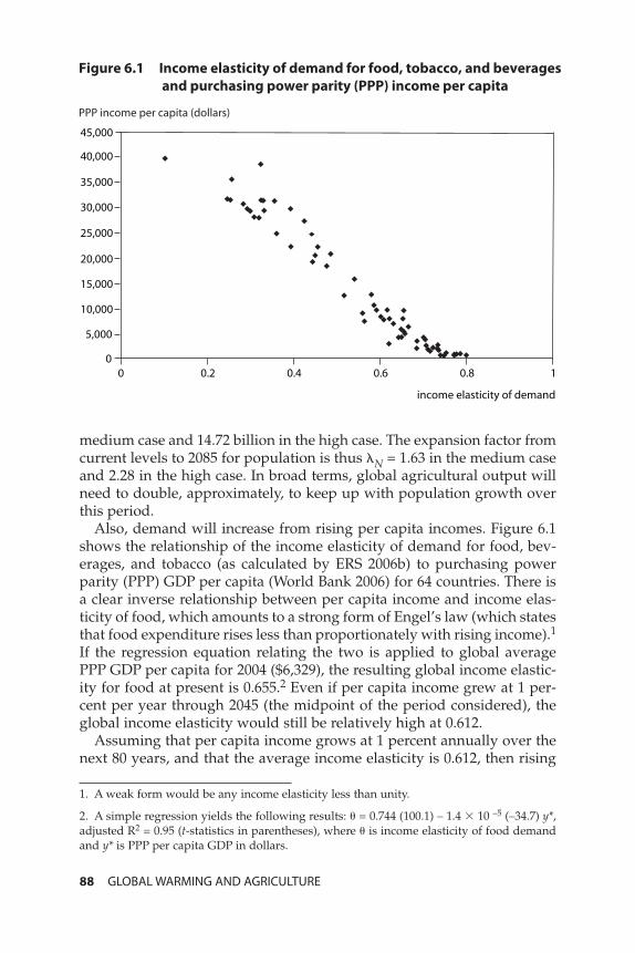
medium case and 14.72 billion in the high case. The expansion factor fromcurrent levels to 2085 for population is thus N = 1.63 in the medium caseand 2.28 in the high case. In broad terms, global agricultural output willneed to double, approximately, to keep up with population growth overthis period.
Also, demand will increase from rising per capita incomes. Figure 6.1shows the relationship of the income elasticity of demand for food, bev-erages, and tobacco (as calculated by ERS 2006b) to purchasing powerparity (PPP) GDP per capita (World Bank 2006) for 64 countries. There isa clear inverse relationship between per capita income and income elas-ticity of food, which amounts to a strong form of Engel’s law (which statesthat food expenditure rises less than proportionately with rising income).1
If the regression equation relating the two is applied to global averagePPP GDP per capita for 2004 ($6,329), the resulting global income elastic-ity for food at present is 0.655.2 Even if per capita income grew at 1 per-cent per year through 2045 (the midpoint of the period considered), theglobal income elasticity would still be relatively high at 0.612.
Assuming that per capita income grows at 1 percent annually over thenext 80 years, and that the average income elasticity is 0.612, then rising
88 GLOBAL WARMING AND AGRICULTURE
1. A weak form would be any income elasticity less than unity.
2. A simple regression yields the following results: � = 0.744 (100.1) – 1.4 � 10 –5 (–34.7) y*,adjusted R2 = 0.95 (t-statistics in parentheses), where � is income elasticity of food demandand y* is PPP per capita GDP in dollars.
Figure 6.1 Income elasticity of demand for food, tobacco, and beverages and purchasing power parity (PPP) income per capita
PPP income per capita (dollars)
0
5,000
10,000
15,000
20,000
25,000
30,000
35,000
40,000
45,000
0 0.2 0.4 0.6
income elasticity of demand
0.8 1
01--Chs. 1-7--1-98 6/28/07 1:19 PM Page 88

income per capita should boost demand for food by a factor of y = 1.63,coincidentally the same as the medium population expansion factor.3
Total demand for food at unchanged real prices would thus rise by afactor that is the multiple of the expansion factor for population and theexpansion factor for per capita income, or D = N y = 1.63 � 1.63 = 2.66for the medium population growth case and 2.28 � 1.63 = 3.72 for the highpopulation growth case.
On the supply side, one positive influence and two negative influencescan be identified. The positive influence is secular rise in yield from tech-nological change. The negative influences are diversion of agriculturalland from food production to the production of energy crops and (cer-tainly by 2085) the impact of global warming.
For land diversion to biomass, a recent study of future energy tech-nologies by the International Energy Agency states the following (IEA2006, 289):
Conventional biofuel production requires about 1% of all arable land and yieldsabout 1% of global transportation fuels. If 100% of the fuel requirements for worldtransport were derived from conventional biofuels, the land requirement wouldreach 1.4 gigahectares, an amount equivalent to all of the world’s arable land. Forthis reason, even if large existing portions of pasture land could be converted tocropland, competition among conventional biofuel production and food produc-tion appears to be inevitable.
The study also notes that sugarcane ethanol is already (more than) com-petitive with oil at $60 per barrel, that grain ethanol (e.g., from maize)would be competitive in relatively large volumes by 2030, and that ligno-celluloic ethanol from such crops as switch grass would be competitive inlarge volumes by 2050. On this basis, it seems reasonable to expect thatabout one-third or more of agricultural land would be devoted to ethanolby the middle of this century. This means that from the standpoint of di-version of land to biomass for energy, the agricultural supply expansionfactor for other crops from the present to the 2080s would be less thanunity, at perhaps B = 0.7.
To examine the prospects for rising agricultural yields from technolog-ical change, it is useful to review the record of the past few decades for the major crops and the major producers. Table 6.1 first presents estimatesof production of the four most important grains, for the 21 largest-producing countries. The data are annual averages for 2001–04.
By identifying the principal world producers of each major crop, table6.1 provides a basis for focusing the analysis of trends in agriculturalyields on the most important producing countries for each product in
DYNAMIC CONSIDERATIONS 89
3. That is, demand for food per capita would rise at the rate of income growth per capitamultiplied by the income elasticity of demand for food, or 1% � 0.612. The expansion factoris thus y = 1.0061280 = 1.629.
01--Chs. 1-7--1-98 6/28/07 1:19 PM Page 89
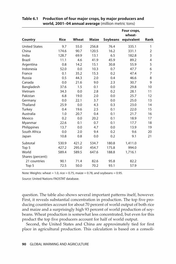
question. The table also shows several important patterns itself, however.First, it reveals substantial concentration in production. The top five pro-ducing countries account for about 70 percent of world output of both riceand maize and a surprisingly high 93 percent of world production of soy-beans. Wheat production is somewhat less concentrated, but even for thisproduct the top five producers account for half of world output.
Second, the United States and China are approximately tied for firstplace in agricultural production. This calculation is based on a consoli-
90 GLOBAL WARMING AND AGRICULTURE
Table 6.1 Production of four major crops, by major producers andworld, 2001–04 annual average (million metric tons)
Four crops,wheat-
Country Rice Wheat Maize Soybeans equivalent Rank
United States 9.7 55.0 256.8 76.4 335.1 1China 174.6 90.7 120.5 16.2 331.1 2India 128.7 69.9 13.1 6.5 182.8 3Brazil 11.1 4.6 41.9 45.9 89.2 4Argentina 0.8 14.2 15.1 30.8 55.9 5Indonesia 52.0 0.0 10.3 0.7 47.7 6France 0.1 35.2 15.3 0.2 47.4 7Russia 0.5 44.3 2.0 0.4 46.6 8Canada 0.0 21.6 9.0 2.3 30.7 9Bangladesh 37.6 1.5 0.1 0.0 29.8 10Vietnam 34.3 0.0 2.8 0.2 28.1 11Pakistan 6.8 19.0 2.0 0.0 25.7 12Germany 0.0 22.1 3.7 0.0 25.0 13Thailand 25.9 0.0 4.3 0.3 23.0 14Turkey 0.4 19.6 2.5 0.1 22.0 15Australia 1.0 20.7 0.4 0.1 21.7 16Mexico 0.2 0.0 20.2 0.1 18.9 17Myanmar 22.6 0.1 0.7 0.1 17.7 18Philippines 13.7 0.0 4.7 0.0 13.9 19South Africa 0.0 2.0 9.4 0.2 9.6 20Japan 10.8 0.8 0.0 0.2 9.1 21
Subtotal 530.9 421.2 534.7 180.8 1,411.0Top 5 427.2 295.0 454.7 175.8 994.0World 589.4 589.5 647.6 188.8 1,716.1Shares (percent):
21 countries 90.1 71.4 82.6 95.8 82.2Top 5 72.5 50.0 70.2 93.1 57.9
Note: Weights: wheat = 1.0, rice = 0.75, maize = 0.78, and soybeans = 0.95.
Source: United Nations FAOSTAT database.
01--Chs. 1-7--1-98 6/28/07 1:19 PM Page 90
dated wheat-equivalent total of output for the four crops, weighting byaverage world prices in 2002–05.4
Third, again using the consolidated wheat-equivalent, world output is approximately 1.7 billion metric tons for the four major grains, or about264 kg per person annually (723 grams per day).5
Fourth, dietary differences are evident in the table, with heavy relianceon rice in Asia and much greater reliance on wheat and maize in the West-ern Hemisphere and Europe.
With this rough summary of global agricultural production in hand,relative country weights in production of key commodities can be appliedto country-specific estimates of the pace of technological change to arriveat broad aggregates for technological change in global agriculture. Table6.2 reports average annual yield increases for these crops in each of theirmajor producing countries for 1961–83 and 1984–2005. These rates are es-timated using statistical regressions of the logarithm of yield per hectareon time and thus avoid distortion by choice of endpoints.6
For each crop, the weighted average pace of increasing yield is obtainedby weighting the production shares of the respective countries in the setof major producers examined. The countries are selected for each cropbased on the top producing countries shown in table 6.1.
In order to obtain an overall rate of yield increase for the four crops, theweighted averages for each commodity are in turn weighted by the shareof the product in global wheat-equivalent production as indicated in table6.1. The result is a central estimate that these agricultural yields rose at anannual rate of 2.81 percent in 1961–83 and decelerated to an annual in-crease of 1.57 percent during 1984–2005. This trend is consistent with thestylized fact that globally the green revolution has slowed down some-what since its heyday in the 1960s.
The final element is now in place for comparing the expansion of agri-cultural demand through late in the 21st century against the correspond-ing prospective expansion in supply. Assuming that the pace of increas-ing yields continues at its rate of the past two decades, or 1.57 percent,
DYNAMIC CONSIDERATIONS 91
4. Average prices in this period, per metric ton, were $132.5 for wheat, $98.8 for rice, $103.7for maize, and $125.9 for soybeans (IMF 2006).
5. Note that the corresponding “food quantity” estimates in the Food and Agriculture Or-ganization (FAO) data are substantially smaller. For the United States, for example, the FAOestimate under this concept is a total of 692 grams per person per day for four grains (rice,wheat, maize, and soybeans) and three meat types (bovine, chicken, and pig). For India, thecorresponding total is only 472 grams (UN FAOSTAT database). The difference from thehigher cereal production total reflects primarily the high ratio of grains to meat productionfor feedgrains, as discussed later.
6. All of the estimates are statistically significant at the 95 percent level or above except forwheat in Australia in both periods.
01--Chs. 1-7--1-98 6/28/07 1:19 PM Page 91
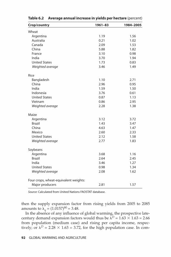
92 GLOBAL WARMING AND AGRICULTURE
Table 6.2 Average annual increase in yields per hectare (percent)
Crop/country 1961–83 1984–2005
WheatArgentina 1.19 1.56Australia 0.21 1.02Canada 2.09 1.53China 5.88 1.82France 3.10 0.98India 3.70 1.94United States 1.73 0.83Weighted average 3.46 1.49
RiceBangladesh 1.10 2.71China 2.96 0.95India 1.59 1.50Indonesia 3.76 0.61United States 0.87 1.13Vietnam 0.86 2.95Weighted average 2.28 1.38
MaizeArgentina 3.12 3.72Brazil 1.43 3.47China 4.63 1.47Mexico 2.60 2.33United States 2.12 1.58Weighted average 2.77 1.83
SoybeansArgentina 3.68 1.16Brazil 2.64 2.45India 3.46 1.27United States 0.98 1.34Weighted average 2.08 1.62
Four crops, wheat-equivalent weights:Major producers 2.81 1.57
Source: Calculated from United Nations FAOSTAT database.
then the supply expansion factor from rising yields from 2005 to 2085amounts to q = (1.0157)80 = 3.48.
In the absence of any influence of global warming, the prospective late-century demand expansion factors would thus be D = 1.63 � 1.63 = 2.66from population (medium case) and rising per capita income, respec-tively; or D = 2.28 � 1.63 = 3.72, for the high population case. In com-
01--Chs. 1-7--1-98 6/28/07 1:19 PM Page 92
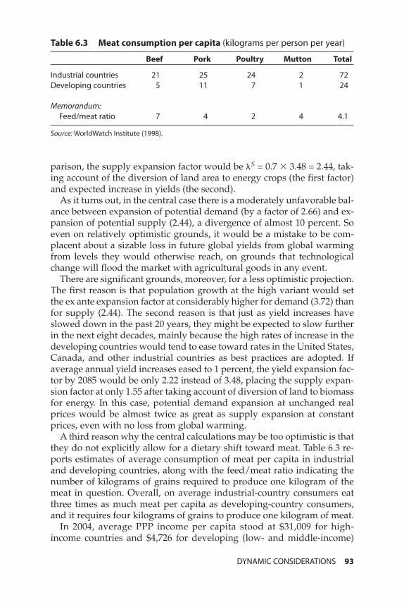
parison, the supply expansion factor would be S = 0.7 � 3.48 = 2.44, tak-ing account of the diversion of land area to energy crops (the first factor)and expected increase in yields (the second).
As it turns out, in the central case there is a moderately unfavorable bal-ance between expansion of potential demand (by a factor of 2.66) and ex-pansion of potential supply (2.44), a divergence of almost 10 percent. Soeven on relatively optimistic grounds, it would be a mistake to be com-placent about a sizable loss in future global yields from global warmingfrom levels they would otherwise reach, on grounds that technologicalchange will flood the market with agricultural goods in any event.
There are significant grounds, moreover, for a less optimistic projection.The first reason is that population growth at the high variant would setthe ex ante expansion factor at considerably higher for demand (3.72) thanfor supply (2.44). The second reason is that just as yield increases haveslowed down in the past 20 years, they might be expected to slow furtherin the next eight decades, mainly because the high rates of increase in thedeveloping countries would tend to ease toward rates in the United States,Canada, and other industrial countries as best practices are adopted. Ifaverage annual yield increases eased to 1 percent, the yield expansion fac-tor by 2085 would be only 2.22 instead of 3.48, placing the supply expan-sion factor at only 1.55 after taking account of diversion of land to biomassfor energy. In this case, potential demand expansion at unchanged realprices would be almost twice as great as supply expansion at constantprices, even with no loss from global warming.
A third reason why the central calculations may be too optimistic is thatthey do not explicitly allow for a dietary shift toward meat. Table 6.3 re-ports estimates of average consumption of meat per capita in industrialand developing countries, along with the feed/meat ratio indicating thenumber of kilograms of grains required to produce one kilogram of themeat in question. Overall, on average industrial-country consumers eatthree times as much meat per capita as developing-country consumers,and it requires four kilograms of grains to produce one kilogram of meat.
In 2004, average PPP income per capita stood at $31,009 for high-income countries and $4,726 for developing (low- and middle-income)
DYNAMIC CONSIDERATIONS 93
Table 6.3 Meat consumption per capita (kilograms per person per year)
Beef Pork Poultry Mutton Total
Industrial countries 21 25 24 2 72Developing countries 5 11 7 1 24
Memorandum:Feed/meat ratio 7 4 2 4 4.1
Source: WorldWatch Institute (1998).
01--Chs. 1-7--1-98 6/28/07 1:19 PM Page 93

countries (World Bank 2006). As a first approximation, then, approxi-mately a sevenfold rise in real per capita income ($31,009 / $4,726 = 6.56)might be expected to generate a threefold rise in per capita consumptionof meat (72/24, from table 6.3), with some attendant reduction in directconsumption of grains (likely especially rice). Correspondingly, if on av-erage developing countries’ real per capita incomes were to rise at 1 per-cent annually over the next eight decades, for an increase by a factor of2.22, their meat consumption per capita could be expected to rise by a fac-tor of approximately 1.6.7
These specific calculations somewhat surprisingly give almost an iden-tical increase in demand for meat in developing countries as that obtainedfor all food applying the estimated income elasticity of 0.612, which inturn would have the implausible implication that rising income wouldnot shift the composition of demand toward meat. So the main calcula-tions of this chapter may not be seriously biased from this standpoint, butif there is a bias, it still seems likely that it is toward an understatement ofthe rise in demand for crop production because of a failure to take specialaccount of shifting demand toward grain-intensive meat.
In short, the principal uncertainties in the estimates of expansion factorsabove are all on the side of downside risk to the late-century balance be-tween potential agricultural demand and supply. These considerations re-inforce the main conclusion that future technological change is no panaceafor addressing concerns about the adverse impact of global warming.
94 GLOBAL WARMING AND AGRICULTURE
7. With c = y where c is per capita meat consumption, y is real PPP income per capita, and hand d refer to high-income and developing countries, respectively, then ch/cd = 3 when yh/yd =6.56 implies that = 0.58 and thus that a rise in developing-country income per capita (yd) bya factor of 2.22 would boost per capita consumption of meat in developing countries by thefactor 2.22 0.58 = 1.59.
01--Chs. 1-7--1-98 6/28/07 1:19 PM Page 94

7Conclusion
This study has applied what might be called a consensus estimate by sixclimate models of changes in temperature and precipitation by 2070–99,by averaging their results as converted to a standardized grid size of 2°latitude by 3° longitude. Models relating agricultural impact to tempera-ture and precipitation (mostly of the Ricardian variety) have then beenapplied to these changes at the standardized grid level and averaged toobtain agricultural impacts at the level of more than 100 countries, re-gions, or subzones within the largest countries. Projections of agriculturalimpact from a suite of alternative crop models and climate models havealso served as the second framework for examining future agriculturalimpact of unabated global warming.
The two central results of these estimates are, first, that at least modestglobal agricultural damage can be expected from business as usual cli-mate change by late in this century, with losses about 15 percent greater ifthe carbon fertilization effect fails to materialize; and second, the damageswill be disproportionately concentrated in developing countries. The di-agnosis of damage suggests that it would be a risky strategy to do noth-ing about global warming on grounds that some studies have estimatedthat there would be global agricultural gains rather than losses for thefirst few degrees of warming. The magnitude of global land surfacewarming by the 2080s under business as usual warming would be 4.4°C(weighting by farm area), and precipitation would rise only 2.9 percent(table 4.3). This combination would go far beyond optimal temperaturesin the low latitudes and also in the mid-latitudes.
Table 7.1 presents an overview of the aggregate estimates of this study.The estimate for global productive capacity change including carbon fer-tilization is a decrease of about 3 percent. This reduction probably under-states potential losses, however. If the carbon fertilization effect (already
95
01--Chs. 1-7--1-98 6/28/07 1:19 PM Page 95
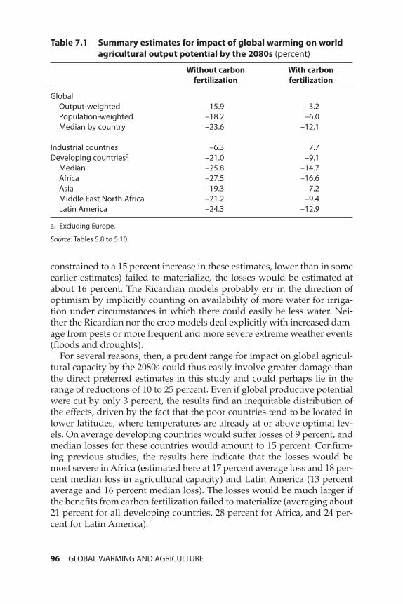
constrained to a 15 percent increase in these estimates, lower than in someearlier estimates) failed to materialize, the losses would be estimated atabout 16 percent. The Ricardian models probably err in the direction ofoptimism by implicitly counting on availability of more water for irriga-tion under circumstances in which there could easily be less water. Nei-ther the Ricardian nor the crop models deal explicitly with increased dam-age from pests or more frequent and more severe extreme weather events(floods and droughts).
For several reasons, then, a prudent range for impact on global agricul-tural capacity by the 2080s could thus easily involve greater damage thanthe direct preferred estimates in this study and could perhaps lie in therange of reductions of 10 to 25 percent. Even if global productive potentialwere cut by only 3 percent, the results find an inequitable distribution ofthe effects, driven by the fact that the poor countries tend to be located inlower latitudes, where temperatures are already at or above optimal lev-els. On average developing countries would suffer losses of 9 percent, andmedian losses for these countries would amount to 15 percent. Confirm-ing previous studies, the results here indicate that the losses would bemost severe in Africa (estimated here at 17 percent average loss and 18 per-cent median loss in agricultural capacity) and Latin America (13 percentaverage and 16 percent median loss). The losses would be much larger ifthe benefits from carbon fertilization failed to materialize (averaging about21 percent for all developing countries, 28 percent for Africa, and 24 per-cent for Latin America).
96 GLOBAL WARMING AND AGRICULTURE
Table 7.1 Summary estimates for impact of global warming on worldagricultural output potential by the 2080s (percent)
Without carbon With carbon fertilization fertilization
GlobalOutput-weighted –15.9 –3.2Population-weighted –18.2 –6.0Median by country –23.6 –12.1
Industrial countries –6.3 7.7Developing countriesa –21.0 –9.1
Median –25.8 –14.7Africa –27.5 –16.6Asia –19.3 –7.2Middle East North Africa –21.2 –9.4Latin America –24.3 –12.9
a. Excluding Europe.
Source: Tables 5.8 to 5.10.
01--Chs. 1-7--1-98 6/28/07 1:19 PM Page 96
In terms of geopolitics, the results here are particularly important for thecases of China and India. China is already the second-largest emitter ofcarbon dioxide (after the United States but ahead of the European Union),and its cooperation will surely be crucial to effective action against globalwarming. Although the central estimate in this study finds China a mod-est gainer in agriculture under business as usual (increase in agriculturalcapacity by about 7 percent with carbon fertilization), the estimate turns toa loss (7 percent reduction in agricultural capacity) if carbon fertilizationeffects do not materialize or are offset by excluded damages. For India,there is no ambiguity: Prospective losses are massive (on the order of 30 to40 percent).
For Australia, one of the two steadfast opponents of the principal inter-national initiative to date against global warming (the Kyoto Protocol),the results also suggest that a more positive position on global warmingabatement would be in its long-term interests. The estimates for Australiaindicate losses of around 16 percent even with carbon fertilization (withpotentially much larger losses suggested by the Ricardian estimates). Asfor the United States, the other principal opponent, although the esti-mates show an aggregate gain of 8 percent in the case with carbon fertil-ization, they indicate a comparable loss (6 percent) if carbon fertilizationis excluded. Moreover, regional losses are pronounced: by about 30 to 35percent in the Southeast and in the Southwest Plains, if carbon fertiliza-tion is excluded (and about 20 to 25 percent if it is included; table 5.8).
For an initial phase of modest global warming, average impacts on agri-culture are ambiguous and may be benign globally on average, but itwould be a serious mistake to infer from such a diagnosis that littleshould be done to curb climate change. This study has sought to sharpenanalysis of agricultural impacts by bringing to bear rigorous and detailedestimates available for regional climate change and quantitative modelsof agricultural impact. The new estimates in this study strongly suggestthat by late in the present century the global effects under business asusual global warming would turn malignant for agriculture globally andthat the damages would be the most severe and begin the soonest wherethey can least be afforded: in the developing countries. Moreover, itwould be a serious mistake to downplay the risks of future agriculturallosses from global warming on grounds that technological change, for ex-ample in new seed varieties, will offset any negative climatic effects. Aclose look at the pace of yield increases in the past two decades, combinedwith attention to the prospective rise in global food demand and the con-version of a substantial portion of agricultural land from food to energycrops, suggests that there is little margin for complacency about erosionin agricultural potential from global warming.
Finally, it should be emphasized that the estimates of this study under-state potential damages from another crucial standpoint: They take a snap-
CONCLUSION 97
01--Chs. 1-7--1-98 6/28/07 1:19 PM Page 97
shot of time at the 2080s, yet baseline damages could be expected to con-tinue to grow throughout the following two centuries before atmosphericconcentrations of carbon eventually would begin to decline once againfrom mixing into the deep ocean (Cline 1992). Even if carbon emissionscollapsed after the 2080s back to well below today’s levels, the delay ofsome three decades for ocean thermal lag means that the warming and im-pacts estimated in this study would substantially underestimate the even-tual equilibrium warming and damages.
98 GLOBAL WARMING AND AGRICULTURE
01--Chs. 1-7--1-98 6/28/07 1:19 PM Page 98

APPENDICES
02--Appendices--99-168 6/21/07 11:40 AM Page 99

02--Appendices--99-168 6/21/07 11:40 AM Page 100
Appendix AStandardizing Global Grids of Climate Change Data
This appendix describes a technique for standardizing global grids in orderto compare climate data produced by different global circulation models(GCMs). The data of various climate modeling centers, including changesin average temperature and precipitation, are available through the DataDistribution Centre of the Intergovernmental Panel on Climate Change(IPCC).1 Every climate modeling center chooses a grid for its unique GCM,and the resolution in latitude and longitude varies greatly across GCMgrids. To compare current observed climate (the 1961–90 average) and fu-ture climate simulations from multiple sources, the observed and modeloutput data must be scaled to a standard grid (G). The task is to link thestandard grid to the grid of observed data and the grids of six GCMs. Thistask is accomplished through pair-wise mapping to G from each of theother seven grids, resulting in one representation of current global climateand six representations of future global climate scaled to the same grid.Mapping to G from the grid of the CCSR/NIES climate model (MCCSR;Emori et al. 1999) will serve as an example of the standardization process.
G is defined to have 90 latitudes and 120 longitudes; it comprises 10,800cells, each with dimension 2° � 3°, spanning the 180° � 360° of the globe.Each cell is identified by two values, LatIDG ∈ [1, 90] and LngIDG ∈[1, 120]. The cell with LatIDG = 1 and LngIDG = 1 is just below the NorthPole and bordered on its west side by the prime meridian, with LatIDG in-
101
1. The database is available at http://ipcc-ddc.cru.uea.ac.uk (accessed on June 23, 2006). TheWeb site is maintained for the IPCC by the Climate Research Unit, University of East Anglia,United Kingdom.
02--Appendices--99-168 6/21/07 11:40 AM Page 101
creasing southward and LngIDG increasing eastward. MCCSR has 32 lati-tudes and 64 longitudes; its cells are 5.625° � 5.625°, and the cell withidentifiers LatIDM = 1 and LngIDM = 1 also falls alongside the North Poleand prime meridian. With G and MCCSR now defined, a subgrid is createdspecifically for this pair of grids. The subgrid has a finer resolution thanboth G and MCCSR and its subcells can be repeated some number of timesto exactly fill both a cell in G and a cell in MCCSR.
The dimensions of a subcell are determined by the greatest commondivisor (GCD) of the dimensions of a G cell and an MCCSR cell. In the di-rection of latitude:
height of subcell = GCD (2, 5.625) = 0.125°
and similarly for longitude:
width of subcell = GCD (3, 5.625) = 0.375°.
Thus the greatest common subcell is 0.125° � 0.375°. Some additionalsimple calculations characterize the relationship of the subgrid to G andto MCCSR and allow for systematic identification of each unique subcell.Let rG be the number of rows of subcells in a row in G, cG be the numberof columns of subcells in a column in G, rM be the number of rows of sub-cells in a row in MCCSR, and cM be the number of columns of subcells in acolumn in MCCSR. These ratios are calculated as follows:
102 GLOBAL WARMING AND AGRICULTURE
Thus there are 1,382,400 (= 16 � 90 � 8 � 120 = 45 � 32 � 15 � 64) sub-cells in the subgrid.
Each unique subcell is defined by a LatIDM, LngIDM, LatSubID, and LngSubID. The SubID values are determined in reference to the cells inMCCSR, so LatSubID ∈ [1, rM = 45] and LngSubID ∈ [1, cM = 15]. LatSubID and
height G cell
GCD (height G cell, height M cell)rG = = 22
0 12516
.=
width G cell
GCD (width G cell, width M cell)cG = = 33
0 3758
.=
height M cell
GCD (height G cell, height M cell)rM = = 55 625
0 12545
.
.=
width M cell
GCD (width G cell, width M cell)cM = = 55 625
0 37515
.
.=
02--Appendices--99-168 6/21/07 11:40 AM Page 102

LatIDG(LatIDM, LatSubID) =
(LatIDM – 1) + (LatSubID)
if (LatIDM – 1) + (LatSubID)
– (LatIDM – 1) + (LatSubID) = 0
1 + (LatIDM – 1) + (LatSubID)
if (LatIDM – 1) + (LatSubID)
– (LatIDM – 1) + (LatSubID) � 0 1rG
⎛
⎝⎜⎞⎠⎟
rrM
G
⎛
⎝⎜⎞⎠⎟
⎤
⎦⎥⎥
1rG
⎛
⎝⎜⎞⎠⎟
rrM
G
⎛
⎝⎜⎞⎠⎟
⎡
⎣⎢⎢
⎤
⎦⎥⎥
1rG
⎛
⎝⎜⎞⎠⎟
rrM
G
⎛
⎝⎜⎞⎠⎟
⎡
⎣⎢⎢
1rG
⎛
⎝⎜⎞⎠⎟
rrM
G
⎛
⎝⎜⎞⎠⎟
⎤
⎦⎥⎥
1rG
⎛
⎝⎜⎞⎠⎟
rrM
G
⎛
⎝⎜⎞⎠⎟
⎡
⎣⎢⎢
1rG
⎛
⎝⎜⎞⎠⎟
rrM
G
⎛
⎝⎜⎞⎠⎟
LngIDG(LngIDM, LngSubID) =
(LngIDM – 1) + (LngSubID)
if (LngIDM – 1) + (LngSubID)
– (LngIDM – 1) + (LngSubID) = 0
1 + (LngIDM – 1) + (LngSubID)
if (LngIDM – 1) + (LngSubID)
– (LngIDM – 1) + (LngSubID) � 0 1cG
⎛
⎝⎜⎞⎠⎟
rrM
G
⎛
⎝⎜⎞⎠⎟
⎤
⎦⎥⎥
1cG
⎛
⎝⎜⎞⎠⎟
ccM
G
⎛
⎝⎜⎞⎠⎟
⎡
⎣⎢⎢
⎤
⎦⎥⎥
1rG
⎛
⎝⎜⎞⎠⎟
ccM
G
⎛
⎝⎜⎞⎠⎟
⎡
⎣⎢⎢
1cG
⎛
⎝⎜⎞⎠⎟
ccM
G
⎛
⎝⎜⎞⎠⎟
⎤
⎦⎥⎥
1cG
⎛
⎝⎜⎞⎠⎟
ccM
G
⎛
⎝⎜⎞⎠⎟
⎡
⎣⎢⎢
1cG
⎛
⎝⎜⎞⎠⎟
ccM
G
⎛
⎝⎜⎞⎠⎟
LngSubID describe the position of a unique subcell out of 675 (= 45 � 15)possible subcells within an MCCSR cell. Thus LatIDM, LngIDM, LatSubID,and LngSubID together define a unique subcell within the entire MCCSRgrid. A pair of equations takes this four-part subcell address as the inputand returns the two-part address of a G cell, completing the initial map-ping between G and MCCSR. The mapping is expressed as two piece-wisefunctions, one for latitude and one for longitude:
APPENDIX A 103
⎧
⎨
⎪⎪⎪⎪⎪⎪⎪⎪⎪
⎩
⎪⎪⎪⎪⎪⎪⎪⎪⎪
⎧
⎨
⎪⎪⎪⎪⎪⎪⎪⎪⎪
⎩
⎪⎪⎪⎪⎪⎪⎪⎪⎪
02--Appendices--99-168 6/21/07 11:40 AM Page 103

where [ ] is the operator returning only the integer portion of its argument.A change in temperature (dT) and precipitation (dP) from base period
1961–90 to the period 2070–99, simulated by the CCSR/NIES model, is as-sociated with each cell in the MCCSR grid. With the mapping from cells inMCCSR to subcells and then to cells in G completed, it is possible to repre-sent the model-derived changes in climate variables over the standardgrid. A simple average of the climate data in the 128 (= 16 � 8) subcellswithin a G cell is computed, associating a dT and a dP based on the CCSR/NIES simulations with each G cell. Because of the curvature of the earth’ssurface, the area of a subcell of fixed degree dimensions is greater near theequator than near the poles; the area increases with the absolute value oflatitude. However, the difference in the area of a subcell with LatSubID = 1and a subcell with LatSubID = 45 within a given cell is insignificant. There-fore, the average of climate data over the subcells within a G cell does notneed to be weighted by area. The expressions for dT and dP are simply:
LatSubID, LngSubID=1 LatSubID, LngSubID=1
In the case of MCCSR, rG = 16 and cG = 8.The same method is implemented with the five additional GCMs for
which data are available and with the observed 1961–90 data, all dis-tributed by the IPCC. The GCMs are ECHAM4/OPYC3, HadCM3, CSIRO-Mk2, GFDL-R30, and CGCM2, along with CCSR/NIES (see table 4.1 forfull names of these models). Unlike the other GCM grids, in the grid of theHadCM3 model the equator bisects a row of cells rather than falling onthe boundary of two rows. The standardization method can still be ap-plied after shifting and renumbering the latitudes of the HadCM3 grid tocorrect the inconsistency. For all grids, the standardization does becomeslightly unreliable very near the poles. The latitude lines in all of the gridsystems are infinitesimally closer together as the absolute value of lati-tude climbs into the 80s, and some of the grids reach 1° or 2° closer to 90°than others. However, these polar areas are not included in the economicimpact analysis because of the absence of any land that would be eco-nomically relevant under plausible levels of warming. Potentially habit-able land is easily captured within the domain of the standardizationmethod.
104 GLOBAL WARMING AND AGRICULTURE
dPr cG G
r cG G
×∑,
.dT
r cG G
r cG G
×∑,
and
02--Appendices--99-168 6/21/07 11:40 AM Page 104
Appendix B Mapping Grid Cells to Countries
This study’s database of 1961–90 and 2070–99 climates is based on a gridof 2° latitude � 3° longitude cells (standard grid G). Matching these cellswith national borders is done using the publicly available Global Popula-tion Distribution Database (Li 1996).1 This database was created for geo-graphic analysis of global population but also includes a table that maps1° � 1° cells to countries. In cases where parts of more than one country (ora combination of land and ocean) are contained in the same cell, the data-base assigns the cell proportionally—for example, 32 percent of a cell toArgentina, 9 percent to Brazil, and 59 percent to Uruguay. Data on the pro-portional share of each cell in the total area of a given country are also in-cluded—for example, that same cell contains 0.122 percent of Argentina’sland area, 0.011 percent of Brazil’s, and 3.695 percent of Uruguay’s.
Description of the Global PopulationDistribution Database
The database consists of three datasets compiled in dBase IV format.2
The first dataset contains global population in 1990 on a 1° � 1° grid.
105
1. The work was supported by Environment Canada and the United Nations EnvironmentProgram—Global Resource Information Database (UNEP GRID) and conducted at Environ-ment Canada. The second dataset in this source, “GridCtry,” is used here for country assign-ment. The dataset is distributed by the United States Geological Survey EROS Data Center,which is the North American base of the UNEP GRID. The data and information are availableat http://grid2.cr.usgs.gov/globalpop/1-degree/description.php3 and http://grid2.cr.usgs.gov/metadata/unep/grid/gridctry.html.
2. This description of the national population grid database is the same as that provided byits creators but is reformatted for readability.
02--Appendices--99-168 6/21/07 11:40 AM Page 105
The second, used for this study, defines the relationship between gridcells and countries. The third dataset contains data on rural populationdistribution.
Definition of Grid Code Number
Grid code number = ( j * 1000) + i
j: row number starting at 1 for 90°S to 89°S latitude to 180 for 89°N to90°N latitude
i: column number starting at 1 for 180°W to 179°W longitude to 360 for179°E to180°E longitude.
The latitude and longitude of the center of the grid cell are given by
latitude = ( j – 91) + 0.5longitude = (i – 181) + 0.5
Dataset 2 (GridCtry.dbf): Relationship Between Grid Cellsand Countries
Fields:
� Grid Grid code number� Cover-Id Cover ID number
“0”: All covered by sea“1”: Entirely contained in one country“2”: Shared by two countries“3”: Shared by three countries“4”: Shared by four countries“10”: Shared by one country and ocean“20”: Shared by two countries and ocean“30”: Shared by three countries and ocean“40”: Shared by four countries and ocean
� UNCode2 United Nations standard ISO country codes� Country Country/region name� Rate-in-Country (%) Percentage of the area of a country contained
in each grid cell� Rate-in-Grid (%) Percentage of the area of the grid cell occupied
by country or ocean
Number of records: 25,540Number of cells: 12,200Total number of countries: 217
106 GLOBAL WARMING AND AGRICULTURE
02--Appendices--99-168 6/21/07 11:40 AM Page 106
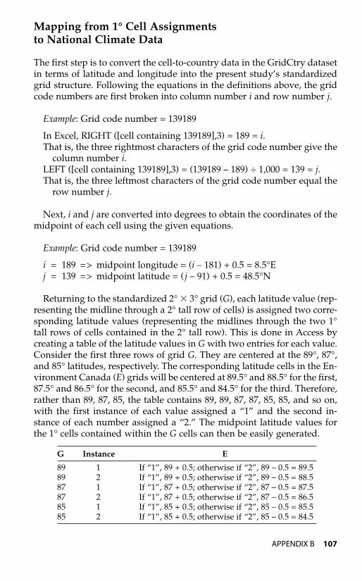
Mapping from 1° Cell Assignments to National Climate Data
The first step is to convert the cell-to-country data in the GridCtry datasetin terms of latitude and longitude into the present study’s standardizedgrid structure. Following the equations in the definitions above, the gridcode numbers are first broken into column number i and row number j.
Example: Grid code number = 139189
In Excel, RIGHT ([cell containing 139189],3) = 189 = i.That is, the three rightmost characters of the grid code number give the
column number i.LEFT ([cell containing 139189],3) = (139189 – 189) ÷ 1,000 = 139 = j.That is, the three leftmost characters of the grid code number equal the
row number j.
Next, i and j are converted into degrees to obtain the coordinates of themidpoint of each cell using the given equations.
Example: Grid code number = 139189
i = 189 => midpoint longitude = (i – 181) + 0.5 = 8.5°Ej = 139 => midpoint latitude = ( j – 91) + 0.5 = 48.5°N
Returning to the standardized 2° � 3° grid (G), each latitude value (rep-resenting the midline through a 2° tall row of cells) is assigned two corre-sponding latitude values (representing the midlines through the two 1°tall rows of cells contained in the 2° tall row). This is done in Access bycreating a table of the latitude values in G with two entries for each value.Consider the first three rows of grid G. They are centered at the 89°, 87°,and 85° latitudes, respectively. The corresponding latitude cells in the En-vironment Canada (E) grids will be centered at 89.5° and 88.5° for the first,87.5° and 86.5° for the second, and 85.5° and 84.5° for the third. Therefore,rather than 89, 87, 85, the table contains 89, 89, 87, 87, 85, 85, and so on,with the first instance of each value assigned a “1” and the second in-stance of each number assigned a “2.” The midpoint latitude values forthe 1° cells contained within the G cells can then be easily generated.
APPENDIX B 107
G Instance E
89 1 If “1”, 89 + 0.5; otherwise if “2”, 89 – 0.5 = 89.589 2 If “1”, 89 + 0.5; otherwise if “2”, 89 – 0.5 = 88.587 1 If “1”, 87 + 0.5; otherwise if “2”, 87 – 0.5 = 87.587 2 If “1”, 87 + 0.5; otherwise if “2”, 87 – 0.5 = 86.585 1 If “1”, 85 + 0.5; otherwise if “2”, 85 – 0.5 = 85.585 2 If “1”, 85 + 0.5; otherwise if “2”, 85 – 0.5 = 84.5
02--Appendices--99-168 6/21/07 11:40 AM Page 107
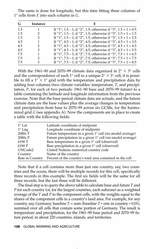
The same is done for longitude, but this time fitting three columns of 1° cells from E into each column in G.
G Instance E
1.5 1 If “1”, 1.5 – 1; if “2”, 1.5; otherwise if “3”, 1.5 + 1 = 0.51.5 2 If “1”, 1.5 – 1; if “2”, 1.5; otherwise if “3”, 1.5 + 1 = 1.51.5 3 If “1”, 1.5 – 1; if “2”, 1.5; otherwise if “3”, 1.5 + 1 = 2.54.5 1 If “1”, 4.5 – 1; if “2”, 4.5; otherwise if “3”, 4.5 + 1 = 3.54.5 2 If “1”, 4.5 – 1; if “2”, 4.5; otherwise if “3”, 4.5 + 1 = 4.54.5 3 If “1”, 4.5 – 1; if “2”, 4.5; otherwise if “3”, 4.5 + 1 = 5.57.5 1 If “1”, 7.5 – 1; if “2”, 7.5; otherwise if “3”, 7.5 + 1 = 6.57.5 2 If “1”, 7.5 – 1; if “2”, 7.5; otherwise if “3”, 7.5 + 1 = 7.57.5 3 If “1”, 7.5 – 1; if “2”, 7.5; otherwise if “3”, 7.5 + 1 = 8.5
With the 1961–90 and 2070–99 climate data organized in 2° � 3° cellsand the correspondence of each 1° cell to a unique 2° � 3° cell, it is possi-ble to fill a 1° � 1° grid with the temperature and precipitation data byadding four columns (two climate variables: temperature, T, and precipi-tation, P, for each of two periods: 1961–90 base and 2070–99 future) to atable containing the latitude and longitude information from the previousexercise. Note that the base period climate data are actuals, and the futureclimate data are the base values plus the average changes in temperatureand precipitation from base to 2070–99 across six GCMs, for the harmo-nized grid G (see appendix A). Now the components are in place to createa table with the following fields:
1° Lat Latitude coordinate of midpoint1° Lng Longitude coordinate of midpoint2080s T Future temperature in a given 1° cell (six-model average)2080s P Future precipitation in a given 1° cell (six-model average)6190 T Base temperature in a given 1° cell (observed)6190 P Base precipitation in a given 1° cell (observed)UNCode2 United Nations numerical country codeCountry Name of the countryRate in Country Percent of the country’s total area contained in the cell
Note that if a cell contains more than just one country, say, two coun-tries and the ocean, there will be multiple records for this cell, specificallythree records in this example. The first six fields will be the same for allthree records, but the last three will be different.
The final step is to query the above table to calculate base and future T andP for each country (or, for the largest countries, each subzone) as a weightedaverage of the T and P in the component cells, with the weights equal to theshares of the component cells in a country’s land area. For example, for anycountry, say, Germany, baseline T = sum (baseline T * rate in country * 0.01),summed over all cells that contain some portion of Germany. The result istemperature and precipitation, for the 1961–90 base period and 2070–99 fu-ture period, in about 220 countries, islands, and territories.
108 GLOBAL WARMING AND AGRICULTURE
02--Appendices--99-168 6/21/07 11:40 AM Page 108
Appendix CCalculating the GeographicalArea of the Grid Cell
For purposes such as estimating global average land surface changes intemperature and precipitation, it is necessary to know the area of the cellsof the grid used in the climate projection. Each cell is an isosceles trape-zoid with parallel top and bottom and sides sloping slightly inward pole-ward. Considering that the distance from pole to pole along any longitu-dinal line is pR where R is the earth’s radius (6,378.17 km), in a grid withvertical resolution of vº and hence 180/v = N rows, the height of eachtrapezoid will be a constant h = (pR)/N.1
The average width of each cell will be the circumference of the circlearound the earth’s surface perpendicular to the earth’s axis at the averagelatitude of the cell in question, divided by the number of columns. Withgrid horizontal resolution of kº, there are 360/k = M columns. At the equa-tor, cell width is (2pR)/M = we. It can be shown that at latitude of degreea (North or South), the circumference of the latitudinal circle around the
109
1. Approximately. Because h as calculated in this way is the length of the vertical side of thetrapezoid rather than the height, or the hypotenuse rather than the height of the right trian-gle having base equal to one-half the difference between cell width at the equatorward sideof the cell and that at the poleward side, true height h* would be slightly smaller. However,the difference is minimal. For example, in the standard grid of this study (90 rows × 120columns), cell height h is 222.64 km. Cell width is 334 km at the equator, 289.2 km at 30ºlatitude, and 167 km at 60º latitude. At this resolution, true cell height is h* = 222.62 km at30º latitude and 222.58 km at 60º latitude, extremely close to the approximation h. Becausethis study’s calculation of country area in each cell area is at a finer 1º × 1º resolution level(see appendix B), any bias is even smaller.
02--Appendices--99-168 7/3/07 11:28 AM Page 109
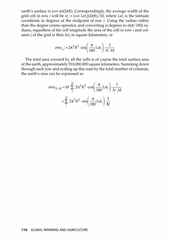
earth’s surface is (cos a)(2pR). Correspondingly, the average width of thegrid cell in row i will be wi = (cos Lati)(2pR)/M, where Lati is the latitudecoordinate in degrees of the midpoint of row i. Using the radian ratherthan the degree cosine operator, and converting a degrees to a(p/180) ra-dians, regardless of the cell longitude the area of the cell in row i and col-umn j of the grid is then hwi in square kilometers, or
The total area covered by all the cells is of course the total surface areaof the earth, approximately 510,000,000 square kilometers. Summing downthrough each row and scaling up this sum by the total number of columns,the earth’s area can be expressed as
area M R LatN MN M i
i
N
, cos= ⋅ ⋅ ⎛⎝⎜
⎞⎠⎟
⋅⋅∑ 2
18012 2π π
= ⋅ ⎛⎝⎜
⎞⎠⎟
⋅2180
12 2π πR Laticos
NNi
N∑
area R LatN Mi j i, cos= ⋅ ⎛
⎝⎜⎞⎠⎟
⋅⋅
2180
12 2π π
110 GLOBAL WARMING AND AGRICULTURE
02--Appendices--99-168 7/3/07 11:28 AM Page 110

Appendix DDefinitions of Countries,Regions, and Subzones
This study estimates agricultural outcomes in 116 countries, regions, andsubzones (CRSs). Seventy of the most populous countries are each in-cluded individually. A region is two or more countries that are smaller (inpopulation terms) and are grouped by geographic proximity, with con-sideration also given to similarity of climate and economy. There are atotal of ten regions composed of 39 countries. Seven countries with largeland area and thus great agricultural significance are broken up into mul-tiple subzones. These countries, with their respective number of sub-zones, are Australia (5), Brazil (3), Canada (5), China (7), India (4), Russia(7), and the United States (7). The subzones are determined by climate,though their boundaries are primarily formed by straight latitude andlongitude lines for simplicity. Table D.1 shows the subzones of the sevenlarge countries, indicating their minimum and maximum coordinates formidpoints of grid cells at 1° resolution. For longitudes, positive figures aredegrees east of the prime meridian, 0 to 180; negative figures are degreeswest of the prime meridian, 0 to –180. For latitudes, positive figures aredegrees north of the equator, 0 to 90; negative figures are degrees south ofthe equator, 0 to –90. Box D.1 lists the countries that constitute regional ag-gregates treated as single CRSs.
111
02--Appendices--99-168 6/21/07 11:40 AM Page 111
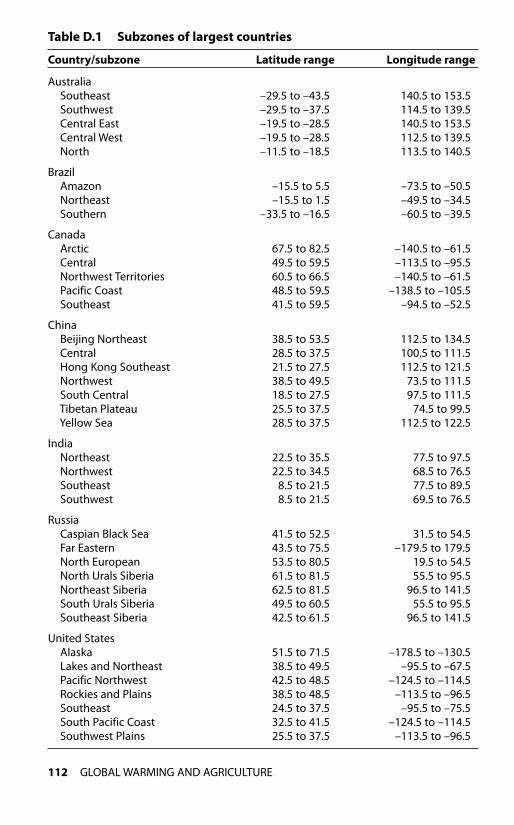
112 GLOBAL WARMING AND AGRICULTURE
Table D.1 Subzones of largest countries
Country/subzone Latitude range Longitude range
AustraliaSoutheast –29.5 to –43.5 140.5 to 153.5Southwest –29.5 to –37.5 114.5 to 139.5Central East –19.5 to –28.5 140.5 to 153.5Central West –19.5 to –28.5 112.5 to 139.5North –11.5 to –18.5 113.5 to 140.5
BrazilAmazon –15.5 to 5.5 –73.5 to –50.5Northeast –15.5 to 1.5 –49.5 to –34.5Southern –33.5 to –16.5 –60.5 to –39.5
CanadaArctic 67.5 to 82.5 –140.5 to –61.5Central 49.5 to 59.5 –113.5 to –95.5Northwest Territories 60.5 to 66.5 –140.5 to –61.5Pacific Coast 48.5 to 59.5 –138.5 to –105.5Southeast 41.5 to 59.5 –94.5 to –52.5
ChinaBeijing Northeast 38.5 to 53.5 112.5 to 134.5Central 28.5 to 37.5 100.5 to 111.5Hong Kong Southeast 21.5 to 27.5 112.5 to 121.5Northwest 38.5 to 49.5 73.5 to 111.5South Central 18.5 to 27.5 97.5 to 111.5Tibetan Plateau 25.5 to 37.5 74.5 to 99.5Yellow Sea 28.5 to 37.5 112.5 to 122.5
IndiaNortheast 22.5 to 35.5 77.5 to 97.5Northwest 22.5 to 34.5 68.5 to 76.5Southeast 8.5 to 21.5 77.5 to 89.5Southwest 8.5 to 21.5 69.5 to 76.5
RussiaCaspian Black Sea 41.5 to 52.5 31.5 to 54.5Far Eastern 43.5 to 75.5 –179.5 to 179.5North European 53.5 to 80.5 19.5 to 54.5North Urals Siberia 61.5 to 81.5 55.5 to 95.5Northeast Siberia 62.5 to 81.5 96.5 to 141.5South Urals Siberia 49.5 to 60.5 55.5 to 95.5Southeast Siberia 42.5 to 61.5 96.5 to 141.5
United StatesAlaska 51.5 to 71.5 –178.5 to –130.5Lakes and Northeast 38.5 to 49.5 –95.5 to –67.5Pacific Northwest 42.5 to 48.5 –124.5 to –114.5Rockies and Plains 38.5 to 48.5 –113.5 to –96.5Southeast 24.5 to 37.5 –95.5 to –75.5South Pacific Coast 32.5 to 41.5 –124.5 to –114.5Southwest Plains 25.5 to 37.5 –113.5 to –96.5
02--Appendices--99-168 6/21/07 11:40 AM Page 112
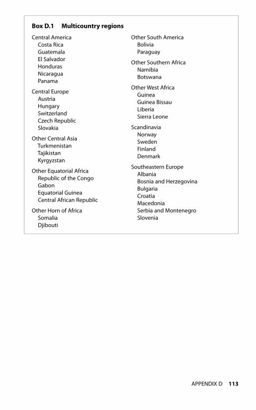
APPENDIX D 113
Box D.1 Multicountry regions
Central AmericaCosta RicaGuatemalaEl SalvadorHondurasNicaraguaPanama
Central EuropeAustriaHungarySwitzerlandCzech RepublicSlovakia
Other Central AsiaTurkmenistanTajikistanKyrgyzstan
Other Equatorial AfricaRepublic of the CongoGabonEquatorial GuineaCentral African Republic
Other Horn of AfricaSomaliaDjibouti
Other South AmericaBoliviaParaguay
Other Southern AfricaNamibiaBotswana
Other West AfricaGuineaGuinea BissauLiberiaSierra Leone
ScandinaviaNorwaySwedenFinlandDenmark
Southeastern EuropeAlbaniaBosnia and HerzegovinaBulgariaCroatiaMacedoniaSerbia and MontenegroSlovenia
02--Appendices--99-168 6/21/07 11:40 AM Page 113

02--Appendices--99-168 6/21/07 11:40 AM Page 114
Appendix EEstimating Farm Area andAgricultural Output byCountry, Region, and Subzone
Agricultural Output
The value of agricultural output in 2003 in millions of US dollars is obtainedby multiplying the dollar value of country GDP (at market prices, not pur-chasing power parity [PPP]) by the percent of GDP reported as originatingin the agricultural sector, as estimated by the World Bank (2005, table 4.2).The exception is for member countries of the Organization for EconomicCooperation and Development (OECD), for which more precise estimatesappear to exist in OECD (2005) and are used here.1 For multicountry re-gions, country-level agricultural output value from the same sources is ag-gregated to obtain the regional total. For subzones within the large coun-tries, attribution of output value is developed as described below.
Geographical Versus Farm Land Area
The geographical land area of each country, region, or subzone is obtainedfrom the mapping methodology described in appendix B. Farmland area
115
1. For the United States, for example, World Bank (2005) reports agricultural output at 2 per-cent of GDP in 2003. The OECD (2005) places it at 0.9 percent. The latter is closer to the valuereported in US national accounts, $88 billion or 0.80 percent in 2003 (BEA 2006, table 1.3.5).
02--Appendices--99-168 6/21/07 11:40 AM Page 115
can be much smaller than geographical area, because of land in forests,mountains, deserts, and other nonfarm areas. The preferred source for thisstudy’s estimate of farm area is the set of country agricultural censusescompiled by the Food and Agriculture Organization (FAO 2006a). For eachcountry, the most recent available agricultural census is used for the esti-mate of land area in farms, typically reported together with the number offarms and distribution by farm size. For numerous countries, census esti-mates are not available. Instead, FAO estimates of “arable land” plus landin “permanent crops” (e.g., fruit trees) are used (FAO 2005). For the 49 in-dividual countries (table 4.2 in chapter 4) for which both sets of FAO dataare available, the median ratio of farm area to total land area is 32.5 per-cent. The median ratio of arable land plus permanent crop land to farmland area is 96.6 percent, although there is wide variation (from 8 percentto around 200 percent), reflecting differences in the data sources. For thelarge agricultural countries, arable land plus permanent crop land tends tobe considerably smaller than farmland area, with the ratio of the former to the latter being about 11 percent in Australia; 20 percent in Argentina,Brazil, and New Zealand; and 47 percent in the United States (but 66 per-cent in France and 77 percent in Canada).
The approach adopted here is simply to accept the larger of the two es-timates (farm land, from the census, or arable land plus land in perma-nent crops) as the best estimate of the relevant farm area in each country.Output per hectare of farm area is then simply the estimate of total agri-cultural output at the country level divided by the estimate of farm areafor the country in question. For multicountry regions, aggregates acrossthe member countries are obtained for farm area and agricultural output.
Subzone Farm Area and Output
Subzone data for farm area and output for the larger countries are rela-tively accessible for Australia, Brazil, China, and the United States but notfor Canada, India, and especially Russia.
For Australia, the Australian Bureau of Statistics (ABS 2005) providesdata on farm area and value of agricultural products sold by province,and for all the provinces there is an obvious mapping to the specific geo-graphical subzone (although for two provinces, the amounts are dividedevenly between the zones they straddle).
For Brazil, data on farm area and output are available by major geo-graphical region from the agricultural census of 1995–96 (IBGE 2006).With minor reallocations, these regions correspond to the subzones usedhere (see appendix D).
For China, a special compilation by the US Department of Agriculture(ERS 2006a) provides data on production (in 2003) and cultivated area (in1996) by province, and for almost all provinces there is an obvious map-
116 GLOBAL WARMING AND AGRICULTURE
02--Appendices--99-168 6/21/07 11:40 AM Page 116

ping to the specific geographical subzone (although for one province theamounts are divided evenly between the two zones it straddles).
For the United States, the agricultural census of 2002 provides state-level data on farm area and value of agricultural products sold (USDA2004). The states map relatively clearly into the subzones used here.2
In all four countries, the proportional distributions of farm area or out-put data from the source in question across the subzones is applied to thecountry total farm area and output estimate from this study to obtain thesubzone farm area and output estimates.
For Canada, Statistics Canada (2007) reports farm area by provincefrom the 2001 agricultural census. The provinces broadly conform to sub-zones used here (but Alberta is divided evenly between Canada Southeastand Canada Pacific Coast). Because the census reports zero farms or farmarea above latitude 60°N, farm area and output for this study’s subzonesCanada Arctic and Canada Northwest Territories are set to zero. In the ab-sence of data on output in each province, it is assumed that the percent-age distribution across provinces is identical for output and farm area.
For India, the US Department of Agriculture (ERS 2006b) indicates thatalmost the entire land area of the country is in cropland. Accordingly, thedirect estimate of the land area in each subzone from the mapping of gridcells in this study provides the basis for the proportional distribution offarm land, and the corresponding hectare amounts are obtained by ap-plying these proportions to the census estimate of India’s total farm area(FAO 2006a). Land area is once again used as a proxy for output, which,as for Canada, results in a uniform estimate of output per hectare for eachsubzone.
Subnational data are least available for Russia. In this case, a rough ap-proximation is made by applying broad ranges for the density of perma-nent crops plus arable land indicated in a country mapping summary bythe FAO (2006b). These ranges are wide, and the point estimate chosen foreach region is set within the respective range such that the aggregate farmland area for Russia as a whole equals a target estimate.3 This estimate inturn is set at twice the FAO (2005) estimate for arable land plus permanentcrops. Arable land and permanent crops are placed at only 7 percent oftotal land area, so even the doubling to include pasture (approximatelythe relationship in the United States) leaves a relatively low estimate forthe amount of farm land in Russia.
APPENDIX E 117
2. Note, however, that Colorado, Kansas, and Utah are each divided evenly between sub-zones US Rockies and Plains and US Southwest and Plains (see table 4.2); Missouri betweenLakes and Northeast and US Southeast; and Oklahoma between US Southeast and USSouthwest and Plains.
3. The resulting fractions of total land area in farms for the subzones used in this study areas follows: Caspian Black Sea, 55 percent; Far Eastern, 5 percent; North European, 20 per-cent; North Urals Siberia, 5 percent; Northeast Siberia, 5 percent; South Urals Siberia, 25 per-cent; and Southeast Siberia, 15 percent.
02--Appendices--99-168 6/21/07 11:40 AM Page 117
Estimates
Table E.1 reports the resulting estimates of farm area and agricultural out-put by country, region, and subzone, as well as total land area for each.Global land area for the countries and regions covered amounts to 12.2billion hectares (122 million square kilometers), or 90 percent of worldland area excluding Antarctica. Global farm area is 3.1 billion hectares, oran average of 25.3 percent of land area. Global agricultural output in 2003amounted to $1.18 trillion at market (not PPP) prices, or about 3.4 percentof gross world product (World Bank 2005).
118 GLOBAL WARMING AND AGRICULTURE
02--Appendices--99-168 6/21/07 11:40 AM Page 118
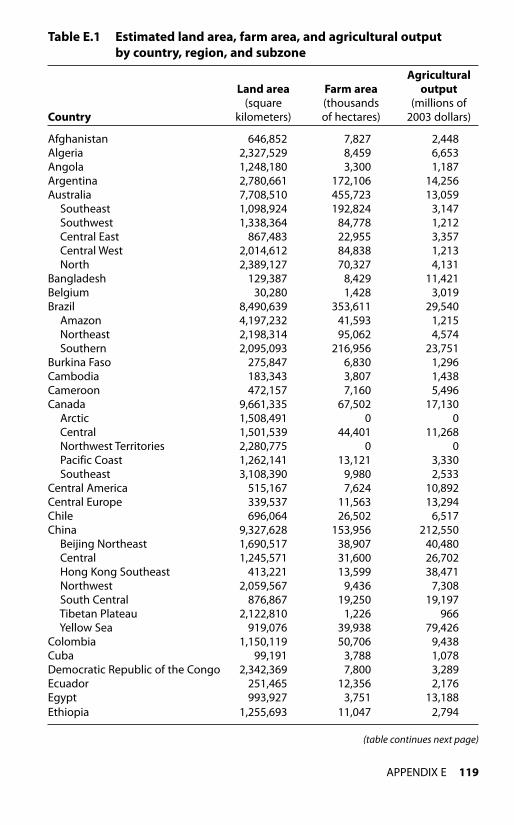
APPENDIX E 119
Table E.1 Estimated land area, farm area, and agricultural outputby country, region, and subzone
AgriculturalLand area Farm area output
(square (thousands (millions ofCountry kilometers) of hectares) 2003 dollars)
Afghanistan 646,852 7,827 2,448Algeria 2,327,529 8,459 6,653Angola 1,248,180 3,300 1,187Argentina 2,780,661 172,106 14,256Australia 7,708,510 455,723 13,059
Southeast 1,098,924 192,824 3,147Southwest 1,338,364 84,778 1,212Central East 867,483 22,955 3,357Central West 2,014,612 84,838 1,213North 2,389,127 70,327 4,131
Bangladesh 129,387 8,429 11,421Belgium 30,280 1,428 3,019Brazil 8,490,639 353,611 29,540
Amazon 4,197,232 41,593 1,215Northeast 2,198,314 95,062 4,574Southern 2,095,093 216,956 23,751
Burkina Faso 275,847 6,830 1,296Cambodia 183,343 3,807 1,438Cameroon 472,157 7,160 5,496Canada 9,661,335 67,502 17,130
Arctic 1,508,491 0 0Central 1,501,539 44,401 11,268Northwest Territories 2,280,775 0 0Pacific Coast 1,262,141 13,121 3,330Southeast 3,108,390 9,980 2,533
Central America 515,167 7,624 10,892Central Europe 339,537 11,563 13,294Chile 696,064 26,502 6,517China 9,327,628 153,956 212,550
Beijing Northeast 1,690,517 38,907 40,480Central 1,245,571 31,600 26,702Hong Kong Southeast 413,221 13,599 38,471Northwest 2,059,567 9,436 7,308South Central 876,867 19,250 19,197Tibetan Plateau 2,122,810 1,226 966Yellow Sea 919,076 39,938 79,426
Colombia 1,150,119 50,706 9,438Cuba 99,191 3,788 1,078Democratic Republic of the Congo 2,342,369 7,800 3,289Ecuador 251,465 12,356 2,176Egypt 993,927 3,751 13,188Ethiopia 1,255,693 11,047 2,794
(table continues next page)
02--Appendices--99-168 6/21/07 11:40 AM Page 119
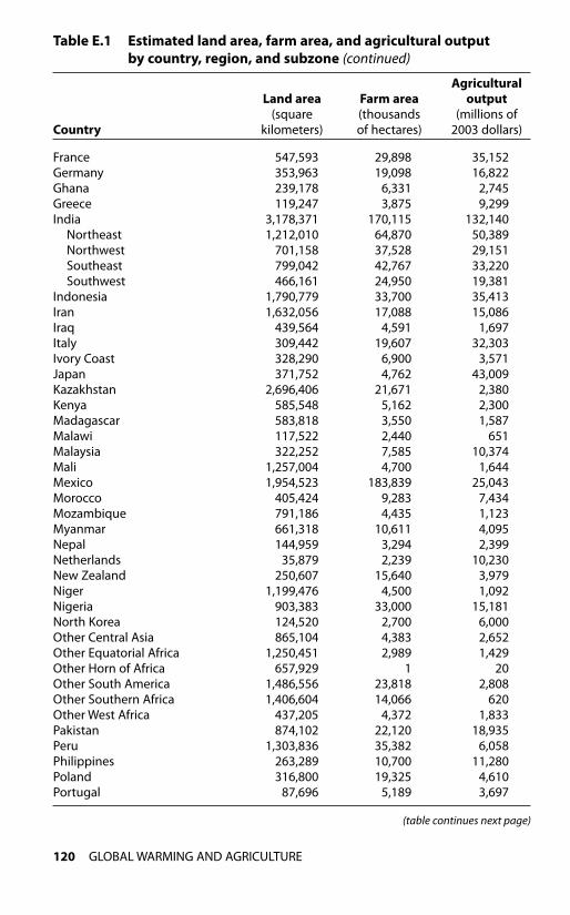
120 GLOBAL WARMING AND AGRICULTURE
France 547,593 29,898 35,152Germany 353,963 19,098 16,822Ghana 239,178 6,331 2,745Greece 119,247 3,875 9,299India 3,178,371 170,115 132,140
Northeast 1,212,010 64,870 50,389Northwest 701,158 37,528 29,151Southeast 799,042 42,767 33,220Southwest 466,161 24,950 19,381
Indonesia 1,790,779 33,700 35,413Iran 1,632,056 17,088 15,086Iraq 439,564 4,591 1,697Italy 309,442 19,607 32,303Ivory Coast 328,290 6,900 3,571Japan 371,752 4,762 43,009Kazakhstan 2,696,406 21,671 2,380Kenya 585,548 5,162 2,300Madagascar 583,818 3,550 1,587Malawi 117,522 2,440 651Malaysia 322,252 7,585 10,374Mali 1,257,004 4,700 1,644Mexico 1,954,523 183,839 25,043Morocco 405,424 9,283 7,434Mozambique 791,186 4,435 1,123Myanmar 661,318 10,611 4,095Nepal 144,959 3,294 2,399Netherlands 35,879 2,239 10,230New Zealand 250,607 15,640 3,979Niger 1,199,476 4,500 1,092Nigeria 903,383 33,000 15,181North Korea 124,520 2,700 6,000Other Central Asia 865,104 4,383 2,652Other Equatorial Africa 1,250,451 2,989 1,429Other Horn of Africa 657,929 1 20Other South America 1,486,556 23,818 2,808Other Southern Africa 1,406,604 14,066 620Other West Africa 437,205 4,372 1,833Pakistan 874,102 22,120 18,935Peru 1,303,836 35,382 6,058Philippines 263,289 10,700 11,280Poland 316,800 19,325 4,610Portugal 87,696 5,189 3,697
Table E.1 Estimated land area, farm area, and agricultural outputby country, region, and subzone (continued)
AgriculturalLand area Farm area output
(square (thousands (millions ofCountry kilometers) of hectares) 2003 dollars)
(table continues next page)
02--Appendices--99-168 6/21/07 11:40 AM Page 120

APPENDIX E 121
Romania 235,076 13,940 6,834Russia 16,661,998 250,182 21,643
Caspian Black Sea 893,762 49,157 4,252Far Eastern 2,373,557 11,868 1,027North European 2,316,608 46,332 4,008North Urals Siberia 2,245,991 11,230 971Northeast Siberia 2,548,377 12,742 1,102South Urals Siberia 2,459,814 61,495 5,320Southeast Siberia 3,823,889 57,358 4,962
Saudi Arabia 1,959,654 4,046 10,737Scandinavia 1,071,983 22,742 9,027Senegal 198,062 2,506 1,104South Africa 1,233,256 15,712 6,395South Korea 88,574 1,877 16,344Southeastern Europe 393,549 13,243 12,566Spain 503,679 42,181 30,191Sri Lanka 57,846 1,916 3,465Sudan 2,520,578 16,653 6,939Syria 186,136 5,421 4,945Tanzania 943,187 10,764 4,634Thailand 513,578 19,367 14,295Turkey 779,877 28,523 26,682Uganda 240,138 7,200 2,015Ukraine 614,704 33,457 6,935United Kingdom 222,153 16,528 12,564United States 9,373,250 379,343 98,537
Alaska 1,448,880 365 23Lakes and Northeast 1,787,870 74,276 30,515Pacific Northwest 603,722 13,117 4,198Rockies and Plains 1,776,216 113,276 15,077Southeast 1,555,232 58,046 22,214South Pacific Coast 716,632 11,170 12,673Southwest Plains 1,484,698 109,094 13,836
Uzbekistan 477,177 4,827 3,482Venezuela 910,829 30,071 3,416Vietnam 316,715 8,895 8,616Yemen 420,297 1,669 1,625Zambia 764,834 5,289 997Zimbabwe 387,668 3,350 3,018
Total 122,294,308 3,097,935 1,175,860
Table E.1 Estimated land area, farm area, and agricultural outputby country, region, and subzone (continued)
AgriculturalLand area Farm area output
(square (thousands (millions ofCountry kilometers) of hectares) 2003 dollars)
02--Appendices--99-168 6/21/07 11:40 AM Page 121

02--Appendices--99-168 6/21/07 11:40 AM Page 122

Appendix FCountry-Level Results with the Mendelsohn-SchlesingerFunctions
The Mendelsohn-Schlesinger models discussed in chapter 5 can be ap-plied to the climate data for the countries, regions, and subzones exam-ined in this study to estimate the impact of global warming on world agri-cultural production. For the carbon fertilization term, the concentration ofatmospheric carbon dioxide used for 2070–99 is the 2085 estimate of 734.5parts per million (ppm) indicated in IPCC (2001a, 807) for scenario SRESA2. That is, by that time atmospheric concentration would approximatelydouble from its 1990 level of 350 ppm.
For application in comparison with recent output, it is necessary tochange the scale of the Mendelsohn-Schlesinger (1999), or MS, functionsto take account of price changes since 1990. The US GDP deflator for thefarm sector has fallen from 155.4 in 1990 to 115.8 in 2003 (with 2000 = 100).Nominal values comparable to the 2003 base year for production thusneed to be reduced to 0.745 times the values obtained directly with theMS functions.
Reduced Form Results
It turns out that the reduced form function generates a high incidence ofnegative estimated output per hectare as a function of temperature andprecipitation even for today’s climate. Of the 116 countries, regions, and
123
02--Appendices--99-168 6/21/07 11:40 AM Page 123
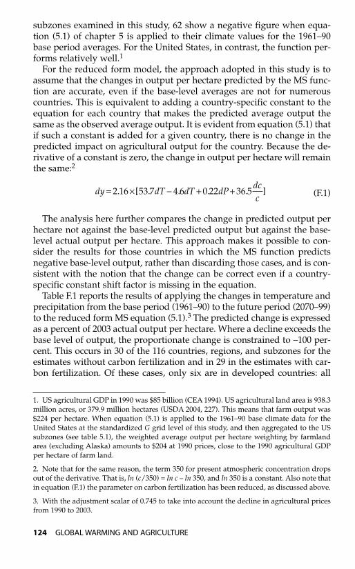
subzones examined in this study, 62 show a negative figure when equa-tion (5.1) of chapter 5 is applied to their climate values for the 1961–90base period averages. For the United States, in contrast, the function per-forms relatively well.1
For the reduced form model, the approach adopted in this study is toassume that the changes in output per hectare predicted by the MS func-tion are accurate, even if the base-level averages are not for numerouscountries. This is equivalent to adding a country-specific constant to theequation for each country that makes the predicted average output thesame as the observed average output. It is evident from equation (5.1) thatif such a constant is added for a given country, there is no change in thepredicted impact on agricultural output for the country. Because the de-rivative of a constant is zero, the change in output per hectare will remainthe same:2
(F.1)
The analysis here further compares the change in predicted output perhectare not against the base-level predicted output but against the base-level actual output per hectare. This approach makes it possible to con-sider the results for those countries in which the MS function predictsnegative base-level output, rather than discarding those cases, and is con-sistent with the notion that the change can be correct even if a country-specific constant shift factor is missing in the equation.
Table F.1 reports the results of applying the changes in temperature andprecipitation from the base period (1961–90) to the future period (2070–99)to the reduced form MS equation (5.1).3 The predicted change is expressedas a percent of 2003 actual output per hectare. Where a decline exceeds thebase level of output, the proportionate change is constrained to –100 per-cent. This occurs in 30 of the 116 countries, regions, and subzones for theestimates without carbon fertilization and in 29 in the estimates with car-bon fertilization. Of these cases, only six are in developed countries: all
dy dT dT dPdcc
= × − + +2 16 53 7 4 6 0 22 36 5. [ . . . . ]
124 GLOBAL WARMING AND AGRICULTURE
1. US agricultural GDP in 1990 was $85 billion (CEA 1994). US agricultural land area is 938.3million acres, or 379.9 million hectares (USDA 2004, 227). This means that farm output was$224 per hectare. When equation (5.1) is applied to the 1961–90 base climate data for theUnited States at the standardized G grid level of this study, and then aggregated to the USsubzones (see table 5.1), the weighted average output per hectare weighting by farmlandarea (excluding Alaska) amounts to $204 at 1990 prices, close to the 1990 agricultural GDPper hectare of farm land.
2. Note that for the same reason, the term 350 for present atmospheric concentration dropsout of the derivative. That is, ln (c/350) = ln c – ln 350, and ln 350 is a constant. Also note thatin equation (F.1) the parameter on carbon fertilization has been reduced, as discussed above.
3. With the adjustment scalar of 0.745 to take into account the decline in agricultural pricesfrom 1990 to 2003.
02--Appendices--99-168 6/21/07 11:40 AM Page 124
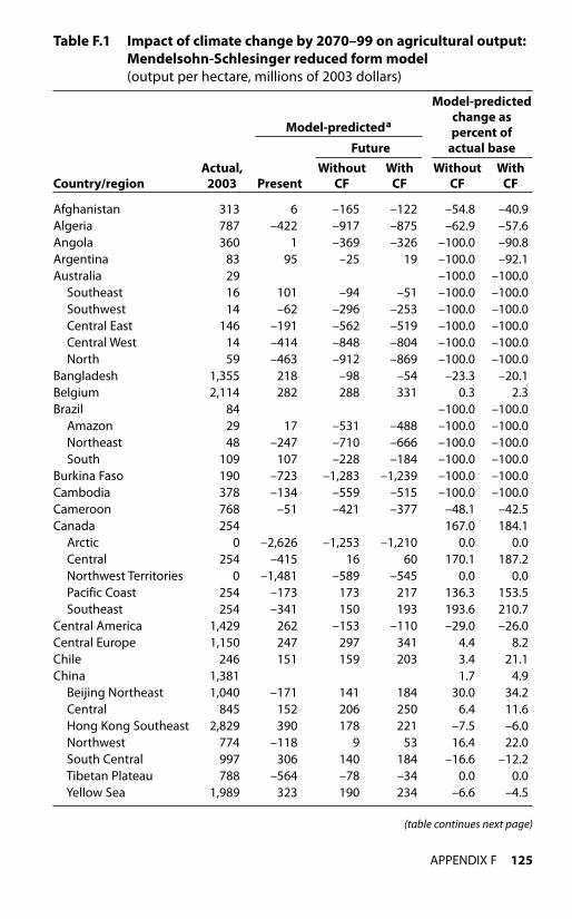
APPENDIX F 125
Table F.1 Impact of climate change by 2070–99 on agricultural output:Mendelsohn-Schlesinger reduced form model (output per hectare, millions of 2003 dollars)
Model-predictedchange aspercent of
Future actual base
Actual, Without With Without WithCountry/region 2003 Present CF CF CF CF
Afghanistan 313 6 –165 –122 –54.8 –40.9Algeria 787 –422 –917 –875 –62.9 –57.6Angola 360 1 –369 –326 –100.0 –90.8Argentina 83 95 –25 19 –100.0 –92.1Australia 29 –100.0 –100.0
Southeast 16 101 –94 –51 –100.0 –100.0Southwest 14 –62 –296 –253 –100.0 –100.0Central East 146 –191 –562 –519 –100.0 –100.0Central West 14 –414 –848 –804 –100.0 –100.0North 59 –463 –912 –869 –100.0 –100.0
Bangladesh 1,355 218 –98 –54 –23.3 –20.1Belgium 2,114 282 288 331 0.3 2.3Brazil 84 –100.0 –100.0
Amazon 29 17 –531 –488 –100.0 –100.0Northeast 48 –247 –710 –666 –100.0 –100.0South 109 107 –228 –184 –100.0 –100.0
Burkina Faso 190 –723 –1,283 –1,239 –100.0 –100.0Cambodia 378 –134 –559 –515 –100.0 –100.0Cameroon 768 –51 –421 –377 –48.1 –42.5Canada 254 167.0 184.1
Arctic 0 –2,626 –1,253 –1,210 0.0 0.0Central 254 –415 16 60 170.1 187.2Northwest Territories 0 –1,481 –589 –545 0.0 0.0Pacific Coast 254 –173 173 217 136.3 153.5Southeast 254 –341 150 193 193.6 210.7
Central America 1,429 262 –153 –110 –29.0 –26.0Central Europe 1,150 247 297 341 4.4 8.2Chile 246 151 159 203 3.4 21.1China 1,381 1.7 4.9
Beijing Northeast 1,040 –171 141 184 30.0 34.2Central 845 152 206 250 6.4 11.6Hong Kong Southeast 2,829 390 178 221 –7.5 –6.0Northwest 774 –118 9 53 16.4 22.0South Central 997 306 140 184 –16.6 –12.2Tibetan Plateau 788 –564 –78 –34 0.0 0.0Yellow Sea 1,989 323 190 234 –6.6 –4.5
(table continues next page)
Model-predicteda
02--Appendices--99-168 6/21/07 11:40 AM Page 125
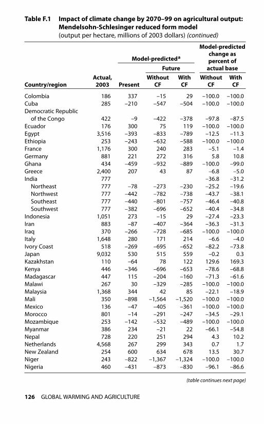
126 GLOBAL WARMING AND AGRICULTURE
Colombia 186 337 –15 29 –100.0 –100.0Cuba 285 –210 –547 –504 –100.0 –100.0Democratic Republic
of the Congo 422 –9 –422 –378 –97.8 –87.5Ecuador 176 300 75 119 –100.0 –100.0Egypt 3,516 –393 –833 –789 –12.5 –11.3Ethiopia 253 –243 –632 –588 –100.0 –100.0France 1,176 300 240 283 –5.1 –1.4Germany 881 221 272 316 5.8 10.8Ghana 434 –459 –932 –889 –100.0 –99.0Greece 2,400 207 43 87 –6.8 –5.0India 777 –36.8 –31.2
Northeast 777 –78 –273 –230 –25.2 –19.6Northwest 777 –442 –782 –738 –43.7 –38.1Southeast 777 –440 –801 –757 –46.4 –40.8Southwest 777 –382 –696 –652 –40.4 –34.8
Indonesia 1,051 273 –15 29 –27.4 –23.3Iran 883 –87 –407 –364 –36.3 –31.3Iraq 370 –266 –728 –685 –100.0 –100.0Italy 1,648 280 171 214 –6.6 –4.0Ivory Coast 518 –269 –695 –652 –82.2 –73.8Japan 9,032 530 515 559 –0.2 0.3Kazakhstan 110 –64 78 122 129.6 169.3Kenya 446 –346 –696 –653 –78.6 –68.8Madagascar 447 115 –204 –160 –71.3 –61.6Malawi 267 30 –329 –285 –100.0 –100.0Malaysia 1,368 344 42 85 –22.1 –18.9Mali 350 –898 –1,564 –1,520 –100.0 –100.0Mexico 136 –47 –405 –361 –100.0 –100.0Morocco 801 –14 –291 –247 –34.5 –29.1Mozambique 253 –142 –532 –489 –100.0 –100.0Myanmar 386 234 –21 22 –66.1 –54.8Nepal 728 220 251 294 4.3 10.2Netherlands 4,568 267 299 343 0.7 1.7New Zealand 254 600 634 678 13.5 30.7Niger 243 –822 –1,367 –1,324 –100.0 –100.0Nigeria 460 –431 –873 –830 –96.1 –86.6
Table F.1 Impact of climate change by 2070–99 on agricultural output:Mendelsohn-Schlesinger reduced form model (output per hectare, millions of 2003 dollars) (continued)
Model-predictedchange aspercent of
Future actual base
Actual, Without With Without WithCountry/region 2003 Present CF CF CF CF
(table continues next page)
Model-predicteda
02--Appendices--99-168 6/21/07 11:40 AM Page 126
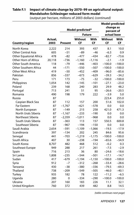
APPENDIX F 127
North Korea 2,222 214 393 437 8.1 10.0Other Central Asia 605 –51 –89 –46 –6.3 0.9Other Equatorial Africa 478 –82 –477 –434 –82.7 –73.6Other Horn of Africa 20,118 –736 –1,160 –1,116 –2.1 –1.9Other South America 118 –79 –446 –403 –100.0 –100.0Other Southern Africa 44 –171 –550 –507 –100.0 –100.0Other West Africa 419 –50 –452 –409 –96.0 –85.6Pakistan 856 –337 –673 –629 –39.3 –34.2Peru 171 173 –75 –32 –100.0 –100.0Philippines 1,054 142 –145 –101 –27.1 –23.0Poland 239 168 240 283 29.9 48.2Portugal 713 241 51 95 –26.6 –20.5Romania 490 198 179 222 –3.9 5.0Russia 87 223.4 255.0
Caspian Black Sea 87 112 157 200 51.6 102.0Far Eastern 87 –1,767 –621 –578 0.0 0.0North European 87 –149 215 258 421.0 471.3North Urals Siberia 87 –1,167 –233 –190 0.0 0.0Northeast Siberia 87 –2,359 –1,011 –968 0.0 0.0South Urals Siberia 87 –363 113 157 550.5 600.8Southeast Siberia 87 –967 –194 –150 0.0 0.0
Saudi Arabia 2,654 –591 –1,109 –1,066 –19.5 –17.9Scandinavia 397 –134 202 245 84.6 95.6Senegal 441 –703 –1,219 –1,175 –100.0 –100.0South Africa 407 30 –238 –194 –65.6 –54.9South Korea 8,707 482 468 512 –0.2 0.3Southeast Europe 949 288 217 261 –7.5 –2.9Spain 716 213 36 80 –24.6 –18.6Sri Lanka 1,808 –235 –544 –501 –17.1 –14.7Sudan 417 –679 –1,194 –1,150 –100.0 –100.0Syria 912 –7 –312 –268 –33.4 –28.6Tanzania 430 –38 –380 –336 –79.5 –69.3Thailand 738 –209 –549 –505 –46.0 –40.1Turkey 935 182 78 122 –11.2 –6.5Uganda 280 0 –334 –290 –100.0 –100.0Ukraine 207 160 183 226 11.1 32.1United Kingdom 760 372 439 482 8.8 14.5
(table continues next page)
Table F.1 Impact of climate change by 2070–99 on agricultural output:Mendelsohn-Schlesinger reduced form model (output per hectare, millions of 2003 dollars) (continued)
Model-predictedchange aspercent of
Future actual base
Actual, Without With Without WithCountry/region 2003 Present CF CF CF CF
Model-predicteda
02--Appendices--99-168 6/21/07 11:40 AM Page 127

five subzones in Australia and one in the United States (Southwest Plains:Arizona, New Mexico, Texas, and parts of Utah, Colorado, Kansas, andOklahoma).4 The results also screen out “ice to ice” cases, where the baseoutput function is highly negative because of low temperature and the fu-ture output function is also negative because temperature remains too lowdespite the warming. Otherwise these areas (e.g., Alaska) would showspurious large gains in agricultural output.
When the percentage changes in agricultural impacts for each country,region, or subzone are applied to the corresponding 2003 benchmark lev-els of agricultural output (see appendix table E.1), the aggregate result is that global agricultural output would fall by $217 billion in the casewithout carbon fertilization and by $152 billion in the case with carbonfertilization. These reductions amount to a reduction in global output by
128 GLOBAL WARMING AND AGRICULTURE
4. Note, however, that the MS reduced form function does not take irrigation into account.
United States 260 –14.8 –2.9Alaska 62 –943 –218 –174 0.0 0.0Lakes, Northeast 411 265 302 346 9.1 19.7Pacific Northwest 320 191 269 313 24.5 38.1Rockies, Plains 133 47 146 190 74.6 107.3Southeast 383 346 86 129 –67.9 –56.6South Pacific Coast 1,135 116 51 95 –5.7 –1.9Southwest Plains 127 80 –159 –116 –100.0 –100.0
Uzbekistan 721 61 –97 –53 –21.8 –15.8Venezuela 114 –9 –441 –398 –100.0 –100.0Vietnam 969 53 –285 –241 –34.9 –30.4Yemen 973 –480 –869 –826 –40.0 –35.5Zambia 189 2 –399 –356 –100.0 –100.0Zimbabwe 901 –79 –455 –412 –41.8 –36.9
Total –18.6 –13.0
CF = carbon fertilization
a. Converted from 1990 to 2003 prices by US farm deflator (0.745).
Note: Total weighting by output (see table 5.8).
Table F.1 Impact of climate change by 2070–99 on agricultural output:Mendelsohn-Schlesinger reduced form model (output per hectare, millions of 2003 dollars) (continued)
Model-predictedchange aspercent of
Future actual base
Actual, Without With Without WithCountry/region 2003 Present CF CF CF CF
Model-predicteda
02--Appendices--99-168 6/21/07 11:40 AM Page 128
18.6 and 13 percent, respectively. On this basis, using the reduced formMS model, global warming would reduce underlying world agriculturalcapacity by about one-fifth to one-eighth from levels otherwise attainableby the 2080s. It should be noted, however, that the only MS reduced formestimates used in the main “preferred” estimates of this study are thosefor the United States, where they are given a weight of one-half alongsideequally weighted results from the Rosenzweig-Iglesias crop models. Forall other country estimates in the crop model framework, the Rosenzweig-Iglesias calculations are used, because they are specifically developed byscientists using agronomic data for the countries and regions in question.
Cross-Section (Ricardian) Results
A corresponding set of estimates can be obtained applying the cross-section (CS) model (equation 5.2 in chapter 5). As discussed in chapter 5,the Ricardian estimates of table F.2 (excluding carbon fertilization) providethe source for the “default” Ricardian estimates in the main text for coun-tries and regions lacking specific estimates. In one sense this set of esti-mates has a more straightforward application than the reduced form (RF)estimates just discussed but in another it requires a more complicated im-plementation. The more straightforward application pertains to the major-ity of observations in which the base level of the agricultural productivitymeasure (rental equivalent opportunity cost of land) is positive. In the CSfunction, only 25 out of 116 cases are negative. So instead of necessarily re-sorting to the “model change relative to actual base” method used for theRF model, where about half the cases show negative base output, it is ap-pealing simply to obtain the percentage change in land rental equivalentvalue by calculating the change in the model estimate against the model es-timate of the base level. For translation into corresponding output changes,this proportionate change in land value (or land rental value) must then bemultiplied by the ratio of net revenue to output (see the discussion for thedirectly estimated regions in chapter 5). For this purpose, the following ra-tios are applied: Africa, 0.78; India and South Asia, 0.67; United States, 0.41;Europe, Japan, Australia, and New Zealand, 0.45; Latin America, 0.50; andAsia and the Middle East, 0.60. The ratios for Africa, India, and the UnitedStates are estimated in chapter 5. For the other regions, intermediate ratiosare set on the basis of relative development level, with the land share pre-sumed to be inversely related to the stage of development. With the per-cent change in output potential in hand, for purposes of global aggregationthis percent change is then applied to each country’s actual base level ofagricultural production. This method is applied to cases “a” in table F.2.
The more complicated dimension pertains to the cases with negativebase estimates, as well as to a subgroup with such low base estimates thatthe model-estimated changes translate into extremely large negative
APPENDIX F 129
02--Appendices--99-168 6/21/07 11:40 AM Page 129
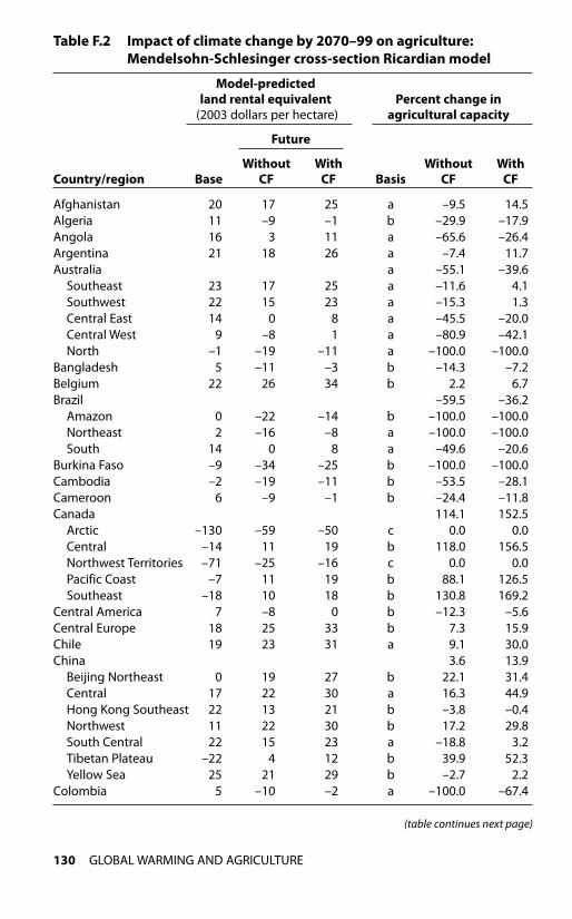
130 GLOBAL WARMING AND AGRICULTURE
Table F.2 Impact of climate change by 2070–99 on agriculture:Mendelsohn-Schlesinger cross-section Ricardian model
Model-predicted land rental equivalent Percent change in
(2003 dollars per hectare) agricultural capacity
Future
Without With Without WithCountry/region Base CF CF Basis CF CF
Afghanistan 20 17 25 a –9.5 14.5Algeria 11 –9 –1 b –29.9 –17.9Angola 16 3 11 a –65.6 –26.4Argentina 21 18 26 a –7.4 11.7Australia a –55.1 –39.6
Southeast 23 17 25 a –11.6 4.1Southwest 22 15 23 a –15.3 1.3Central East 14 0 8 a –45.5 –20.0Central West 9 –8 1 a –80.9 –42.1North –1 –19 –11 a –100.0 –100.0
Bangladesh 5 –11 –3 b –14.3 –7.2Belgium 22 26 34 b 2.2 6.7Brazil –59.5 –36.2
Amazon 0 –22 –14 b –100.0 –100.0Northeast 2 –16 –8 a –100.0 –100.0South 14 0 8 a –49.6 –20.6
Burkina Faso –9 –34 –25 b –100.0 –100.0Cambodia –2 –19 –11 b –53.5 –28.1Cameroon 6 –9 –1 b –24.4 –11.8Canada 114.1 152.5
Arctic –130 –59 –50 c 0.0 0.0Central –14 11 19 b 118.0 156.5Northwest Territories –71 –25 –16 c 0.0 0.0Pacific Coast –7 11 19 b 88.1 126.5Southeast –18 10 18 b 130.8 169.2
Central America 7 –8 0 b –12.3 –5.6Central Europe 18 25 33 b 7.3 15.9Chile 19 23 31 a 9.1 30.0China 3.6 13.9
Beijing Northeast 0 19 27 b 22.1 31.4Central 17 22 30 a 16.3 44.9Hong Kong Southeast 22 13 21 b –3.8 –0.4Northwest 11 22 30 b 17.2 29.8South Central 22 15 23 a –18.8 3.2Tibetan Plateau –22 4 12 b 39.9 52.3Yellow Sea 25 21 29 b –2.7 2.2
Colombia 5 –10 –2 a –100.0 –67.4
(table continues next page)
02--Appendices--99-168 6/21/07 11:40 AM Page 130
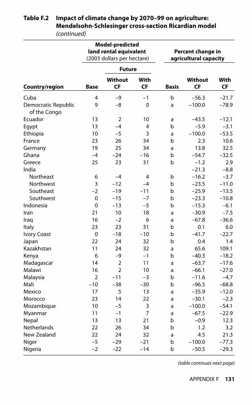
APPENDIX F 131
Table F.2 Impact of climate change by 2070–99 on agriculture:Mendelsohn-Schlesinger cross-section Ricardian model(continued)
Model-predicted land rental equivalent Percent change in
(2003 dollars per hectare) agricultural capacity
Future
Without With Without WithCountry/region Base CF CF Basis CF CF
Cuba 4 –9 –1 b –56.3 –21.7Democratic Republic 9 –8 0 a –100.0 –78.9
of the CongoEcuador 13 2 10 a –43.5 –12.1Egypt 13 –4 4 b –5.9 –3.1Ethiopia 10 –5 3 a –100.0 –53.5France 23 26 34 b 2.3 10.6Germany 19 25 34 a 13.8 32.5Ghana –4 –24 –16 b –54.7 –32.5Greece 25 23 31 b –1.2 2.9India –21.3 –8.8
Northeast 6 –4 4 b –16.2 –3.7Northwest 3 –12 –4 b –23.5 –11.0Southeast –2 –19 –11 b –25.9 –13.5Southwest 0 –15 –7 b –23.3 –10.8
Indonesia 0 –13 –5 b –15.3 –6.1Iran 21 10 18 a –30.9 –7.5Iraq 16 –2 6 a –67.8 –36.6Italy 23 23 31 b 0.1 6.0Ivory Coast 0 –18 –10 b –41.7 –22.7Japan 22 24 32 b 0.4 1.4Kazakhstan 11 24 32 a 65.6 109.1Kenya 6 –9 –1 b –40.3 –18.2Madagascar 14 2 11 a –63.7 –17.6Malawi 16 2 10 a –66.1 –27.0Malaysia 2 –11 –3 b –11.6 –4.7Mali –10 –38 –30 b –96.5 –68.8Mexico 17 5 13 a –35.9 –12.0Morocco 23 14 22 a –30.1 –2.3Mozambique 10 –5 3 a –100.0 –54.1Myanmar 11 –1 7 a –67.5 –22.9Nepal 13 13 21 b –0.9 12.3Netherlands 22 26 34 b 1.2 3.2New Zealand 22 24 32 a 4.5 21.3Niger –5 –29 –21 b –100.0 –77.3Nigeria –2 –22 –14 b –50.5 –29.3
(table continues next page)
02--Appendices--99-168 6/21/07 11:40 AM Page 131
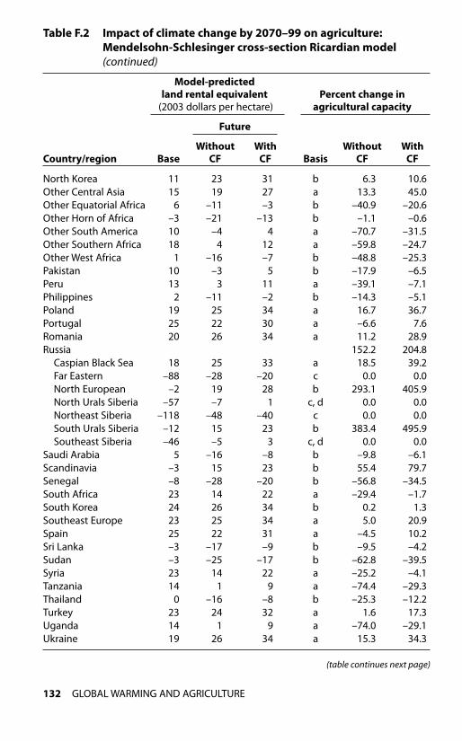
132 GLOBAL WARMING AND AGRICULTURE
North Korea 11 23 31 b 6.3 10.6Other Central Asia 15 19 27 a 13.3 45.0Other Equatorial Africa 6 –11 –3 b –40.9 –20.6Other Horn of Africa –3 –21 –13 b –1.1 –0.6Other South America 10 –4 4 a –70.7 –31.5Other Southern Africa 18 4 12 a –59.8 –24.7Other West Africa 1 –16 –7 b –48.8 –25.3Pakistan 10 –3 5 b –17.9 –6.5Peru 13 3 11 a –39.1 –7.1Philippines 2 –11 –2 b –14.3 –5.1Poland 19 25 34 a 16.7 36.7Portugal 25 22 30 a –6.6 7.6Romania 20 26 34 a 11.2 28.9Russia 152.2 204.8
Caspian Black Sea 18 25 33 a 18.5 39.2Far Eastern –88 –28 –20 c 0.0 0.0North European –2 19 28 b 293.1 405.9North Urals Siberia –57 –7 1 c, d 0.0 0.0Northeast Siberia –118 –48 –40 c 0.0 0.0South Urals Siberia –12 15 23 b 383.4 495.9Southeast Siberia –46 –5 3 c, d 0.0 0.0
Saudi Arabia 5 –16 –8 b –9.8 –6.1Scandinavia –3 15 23 b 55.4 79.7Senegal –8 –28 –20 b –56.8 –34.5South Africa 23 14 22 a –29.4 –1.7South Korea 24 26 34 b 0.2 1.3Southeast Europe 23 25 34 a 5.0 20.9Spain 25 22 31 a –4.5 10.2Sri Lanka –3 –17 –9 b –9.5 –4.2Sudan –3 –25 –17 b –62.8 –39.5Syria 23 14 22 a –25.2 –4.1Tanzania 14 1 9 a –74.4 –29.3Thailand 0 –16 –8 b –25.3 –12.2Turkey 23 24 32 a 1.6 17.3Uganda 14 1 9 a –74.0 –29.1Ukraine 19 26 34 a 15.3 34.3
(table continues next page)
Table F.2 Impact of climate change by 2070–99 on agriculture:Mendelsohn-Schlesinger cross-section Ricardian model(continued)
Model-predicted land rental equivalent Percent change in
(2003 dollars per hectare) agricultural capacity
Future
Without With Without WithCountry/region Base CF CF Basis CF CF
02--Appendices--99-168 6/21/07 11:40 AM Page 132
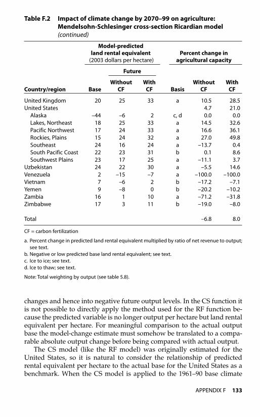
changes and hence into negative future output levels. In the CS function itis not possible to directly apply the method used for the RF function be-cause the predicted variable is no longer output per hectare but land rentalequivalent per hectare. For meaningful comparison to the actual outputbase the model-change estimate must somehow be translated to a compa-rable absolute output change before being compared with actual output.
The CS model (like the RF model) was originally estimated for theUnited States, so it is natural to consider the relationship of predictedrental equivalent per hectare to the actual base for the United States as abenchmark. When the CS model is applied to the 1961–90 base climate
APPENDIX F 133
United Kingdom 20 25 33 a 10.5 28.5United States 4.7 21.0
Alaska –44 –6 2 c, d 0.0 0.0Lakes, Northeast 18 25 33 a 14.5 32.6Pacific Northwest 17 24 33 a 16.6 36.1Rockies, Plains 15 24 32 a 27.0 49.8Southeast 24 16 24 a –13.7 0.4South Pacific Coast 22 23 31 b 0.1 8.6Southwest Plains 23 17 25 a –11.1 3.7
Uzbekistan 24 22 30 a –5.5 14.6Venezuela 2 –15 –7 a –100.0 –100.0Vietnam 7 –6 2 b –17.2 –7.1Yemen 9 –8 0 b –20.2 –10.2Zambia 16 1 10 a –71.2 –31.8Zimbabwe 17 3 11 b –19.0 –8.0
Total –6.8 8.0
CF = carbon fertilization
a. Percent change in predicted land rental equivalent multiplied by ratio of net revenue to output;see text.
b. Negative or low predicted base land rental equivalent; see text.c. Ice to ice; see text.d. Ice to thaw; see text.
Note: Total weighting by output (see table 5.8).
Table F.2 Impact of climate change by 2070–99 on agriculture:Mendelsohn-Schlesinger cross-section Ricardian model(continued)
Model-predicted land rental equivalent Percent change in
(2003 dollars per hectare) agricultural capacity
Future
Without With Without WithCountry/region Base CF CF Basis CF CF
02--Appendices--99-168 6/21/07 11:40 AM Page 133
data, the farm area–weighted average of the estimated land rental equiv-alent for the non-Alaska subzones turns out to be 8.4 percent of the corre-sponding weighted average of actual 2003 output per hectare. On thisbasis, for those country cases in which it is necessary to apply the model-predicted change in land rental equivalent against the base output (ratherthan applying outright the percent change in land rental equivalent), thecorresponding absolute change in output per hectare is simply imputed at12 times the change in the land rental equivalent. The change in outputper hectare is then compared with the base level of output per hectare toobtain the percent change in output potential.5 The criterion chosen forapplication of this alternative calculation, or case “b”, is that the countryin question has a predicted base land rental equivalent per hectare that iseither negative or less than 2 percent of 2003 output per hectare (i.e., one-fourth of the US level). This subset turns out to include 25 cases with neg-ative base predicted land rental equivalent plus another 31 cases in whichthe estimated base is positive but falls below the 2 percent of actual out-put per hectare threshold.
The result is that somewhat fewer than half of the estimates for the CSfunction apply the percent change in the predicted land rental equivalentas translated into percent change in output potential multiplying by theratio of net revenue to output (cases “a” in table F.2). Half apply the alter-native method that first translates the model change into output changeand then compares this absolute change with the actual base (cases “b” inthe table). The remaining cases are “ice to ice,” which as described earlierin the RF results are again set to zero change from global warming.
As expected, the Ricardian CS function results show lower agriculturaldamage from global warming than the crop model–derived RF results(the same comparative outcome found in Mendelsohn and Schlesinger1999 and Mendelsohn et al. 2000). In the aggregate, world agricultural po-tential falls by 6.8 percent without carbon fertilization. In the case withcarbon fertilization, world productive capacity rises by 8 percent.
The CS model damages are only about one-third as large as the RFmodel results, for the case without carbon fertilization. Mendelsohn et al.(2000, 557) suggest that the cross-section damages are smaller because thisapproach “carefully includes adaptation since it captures how people haveadapted to where they live.” This interpretation is somewhat at odds withRichard Adams’ statement that the underlying process-based models de-veloped in Adams et al. (1999)—the basis for the MS reduced form model—already incorporate adaptation. Moreover, considering that Adams et al.suggest that adaptation could offset only about half of the damages frommoderate warming and a lesser amount for larger temperature changes (asnoted earlier), the shrinkage of the global damage estimates from the RF to
134 GLOBAL WARMING AND AGRICULTURE
5. In these cases, there is no need for an additional step of multiplying by the ratio of netrevenue to output.
02--Appendices--99-168 6/21/07 11:40 AM Page 134
the CS estimates here would also seem to overstate the mitigation from ad-ditional adaptation in the CS model. The cutback is considerably morethan half, yet cutback even by half from adaptation would imply that theRF model had incorporated no adaptation at all and in addition that theapproximately 5°C of warming for land areas by the 2080s is “moderate,”which it is not.
The results for the case with carbon fertilization differ considerablymore between the RF and CS models. It should be kept in mind that car-bon fertilization cannot be estimated by statistical regression across re-gions, unlike the rest of the CS function, because all farms face the samepresent-day atmospheric concentration of carbon. Instead, authors mustarbitrarily impose the carbon fertilization parameter. As discussed inchapter 3, the parameter chosen by Mendelsohn and Schlesinger is some-what higher for the CS Ricardian model than for the RF models. Based onthe results of tables F.1 and F.2, implicitly the global weighted effect of car-bon fertilization by the 2080s is to raise yields by 7 percent in the RFmodel but by 16 percent in the CS model.6 In light of the central estimateof the present study of 15 percent yield increase from atmospheric carbonconcentration of 735 ppm by the 2080s, on the basis of the recent free airconcentration enrichment (FACE) studies as discussed earlier, the resultsfor the carbon fertilization case in the MS estimates appear reasonable. Asnoted in chapter 3, however, in their corresponding global estimates(Mendelsohn et al. 2000), the authors substantially increased the carbonfertilization parameter and thus appear to have overstated the carbon fer-tilization effect.7
APPENDIX F 135
6. The multiple of implied future-period productivity with carbon fertilization to that with-out is: (1 – 0.127)/(1 – 0.184) = 1.070 for the RF model (table F.1) and (1 � 0.083)/(1 – 0.066) =1.160 for the Ricardian CS model (table F.2).
7. Note further that the percentage increases discussed here are after the proportionatechange from the CS function for land rental equivalent has been shrunk down to the corre-sponding percent increase in output by applying the ratio of net revenue to output, rangingfrom 0.41 for the United States to 0.78 for Africa. See chapter 3 for further discussion.
02--Appendices--99-168 6/21/07 11:40 AM Page 135

02--Appendices--99-168 6/21/07 11:40 AM Page 136
Appendix GRicardian Models for India,Africa, and Latin America
Mendelsohn, Dinar, and Sanghi (2001) provide a Ricardian climate impactmodel for agriculture in India. Their statistical regression estimates across271 districts, with 10 annual cross-sections for India, are shown in tableG.1. In addition to the climate variables, the model includes the followingcontrol variables: population density, literacy, latitude, high yield, bulls perhectare, tractors per hectare, number of hectares in district, and six soil types.
For Africa, the World Bank recently carried out a survey of 9,597 farmsin Burkina Faso, Egypt, Ethiopia, Ghana, Niger, Senegal, South Africa,Zambia, Cameroon, Kenya, and Zimbabwe. Of the farms surveyed, 7,238had dryland crops, 1,221 had irrigated crops, and 5,062 had livestock (aswell as crops, in most cases). Of the irrigated-crop observations, 58 per-cent were in Egypt. A summary statistical analysis of these data providesRicardian climate functions meant to be representative for Africa (Ku-rukulasuriya et al. 2006). The climate regression coefficients from thisanalysis, for dryland and irrigated agriculture are shown in table G.2. Al-though the analysis also included a model for livestock, it was specifiedin terms of net revenue “per farm” rather than per hectare, a form that istoo ambiguous for meaningful application in the climate impact simula-tions of the present study because of variation in farm size.
As noted earlier in the present study, the Africa models include a vari-ant for irrigated agriculture based only on observations excluding farmsin Egypt. Although the authors do not report the full set of parameters forthat model, they do report the parameters for the marginal impact of tem-perature and precipitation for the model including Egypt (called A) and
137
02--Appendices--99-168 6/21/07 11:40 AM Page 137
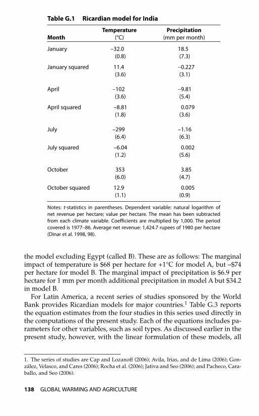
the model excluding Egypt (called B). These are as follows: The marginalimpact of temperature is $68 per hectare for +1°C for model A, but –$74per hectare for model B. The marginal impact of precipitation is $6.9 perhectare for 1 mm per month additional precipitation in model A but $34.2in model B.
For Latin America, a recent series of studies sponsored by the WorldBank provides Ricardian models for major countries.1 Table G.3 reportsthe equation estimates from the four studies in this series used directly inthe computations of the present study. Each of the equations includes pa-rameters for other variables, such as soil types. As discussed earlier in thepresent study, however, with the linear formulation of these models, all
138 GLOBAL WARMING AND AGRICULTURE
1. The series of studies are Cap and Lozanoff (2006); Avila, Irias, and de Lima (2006); Gon-zález, Velasco, and Cares (2006); Rocha et al. (2006); Jativa and Seo (2006); and Pacheco, Cara-ballo, and Seo (2006).
Table G.1 Ricardian model for India
Temperature PrecipitationMonth (°C) (mm per month)
January –32.0 18.5(0.8) (7.3)
January squared 11.4 –0.227(3.6) (3.1)
April –102 –9.81(3.6) (5.4)
April squared –8.81 0.079(1.8) (3.6)
July –299 –1.16(6.4) (6.3)
July squared –6.04 0.002(1.2) (5.6)
October 353 3.85(6.0) (4.7)
October squared 12.9 0.005(1.1) (0.9)
Notes: t-statistics in parentheses. Dependent variable: natural logarithm of net revenue per hectare; value per hectare. The mean has been subtractedfrom each climate variable. Coefficients are multiplied by 1,000. The periodcovered is 1977–86. Average net revenue: 1,424.7 rupees of 1980 per hectare(Dinar et al. 1998, 98).
02--Appendices--99-168 6/21/07 11:40 AM Page 138
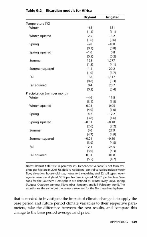
that is needed to investigate the impact of climate change is to apply thebase period and future period climate variables to their respective para-meters, take the difference between the two results, and compare thischange to the base period average land price.
APPENDIX G 139
Table G.2 Ricardian models for Africa
Dryland Irrigated
Temperature (°C)Winter –68 181
(1.1) (1.1)Winter squared 2.5 –3.2
(1.6) (0.6)Spring –28 –180
(0.3) (0.8)Spring squared –1.0 0.8
(0.5) (0.2)Summer 125 1,277
(1.8) (4.1)Summer squared –1.4 –20.2
(1.0) (3.7)Fall –58 –1,517
(0.8) (3.3)Fall squared 0.4 28.7
(0.2) (3.4)Precipitation (mm per month)
Winter –4.6 11.8 (3.4) (1.5)
Winter squared 0.03 –0.05 (4.0) (1.0)
Spring 4.7 –12.2 (3.8) (1.6)
Spring squared –0.01 –0.10 (2.6) (2.2)
Summer 3.6 27.9 (4.7) (4.9)
Summer squared –0.01 –0.10 (3.9) (4.5)
Fall –2.1 25.5 (3.0) (4.3)
Fall squared 0.01 0.08 (5.5) (4.7)
Notes: Robust t-statistic in parentheses. Dependent variable is net farm rev-enue per hectare in 2005 US dollars. Additional control variables include waterflow, elevation, household size, household electricity, and 22 soil types. Aver-age net revenue: dryland, $319 per hectare; irrigated, $1,261 per hectare. Sea-sons for the Southern Hemisphere are defined as: winter (May–July), spring(August–October), summer (November–January), and fall (February–April). Themonths are the same but the seasons reversed for the Northern Hemisphere.
02--Appendices--99-168 6/21/07 11:40 AM Page 139
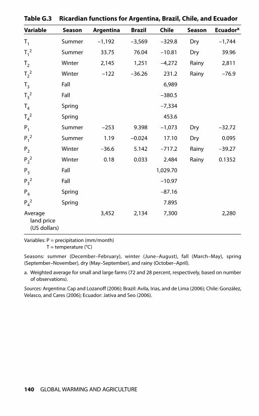
140 GLOBAL WARMING AND AGRICULTURE
Table G.3 Ricardian functions for Argentina, Brazil, Chile, and Ecuador
Variable Season Argentina Brazil Chile Season Ecuadora
T1 Summer –1,192 –3,569 –329.8 Dry –1,744
T12 Summer 33.75 76.04 –10.81 Dry 39.96
T2 Winter 2,145 1,251 –4,272 Rainy 2,811
T22 Winter –122 –36.26 231.2 Rainy –76.9
T3 Fall 6,989
T32 Fall –380.5
T4 Spring –7,334
T42 Spring 453.6
P1 Summer –253 9.398 –1,073 Dry –32.72
P12 Summer 1.19 –0.024 17.10 Dry 0.095
P2 Winter –36.6 5.142 –717.2 Rainy –39.27
P22 Winter 0.18 0.033 2.484 Rainy 0.1352
P3 Fall 1,029.70
P32 Fall –10.97
P4 Spring –87.16
P42 Spring 7.895
Average 3,452 2,134 7,300 2,280land price (US dollars)
Variables: P = precipitation (mm/month)T = temperature (°C)
Seasons: summer (December–February), winter (June–August), fall (March–May), spring (September–November), dry (May–September), and rainy (October–April).
a. Weighted average for small and large farms (72 and 28 percent, respectively, based on numberof observations).
Sources: Argentina: Cap and Lozanoff (2006); Brazil: Avila, Irias, and de Lima (2006); Chile: González,Velasco, and Cares (2006); Ecuador: Jativa and Seo (2006).
02--Appendices--99-168 6/21/07 11:40 AM Page 140
Appendix HMonthly Climate Data, 1961–90 and 2070–99
141
02--Appendices--99-168 6/21/07 11:40 AM Page 141
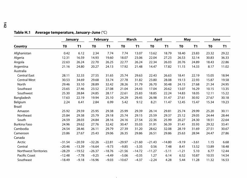
142
Table H.1 Average temperature, January–June (°C)
January February March April May June
Country T0 T1 T0 T1 T0 T1 T0 T1 T0 T1 T0 T1
Afghanistan 0.42 6.12 2.34 7.74 7.74 13.07 13.62 18.79 18.40 23.83 23.32 29.22Algeria 12.31 16.59 14.93 19.60 18.07 23.06 22.04 27.23 26.53 32.14 30.83 36.33Angola 22.63 26.24 22.70 26.25 22.77 26.24 22.34 26.03 20.76 24.89 18.43 22.86Argentina 21.16 24.80 20.27 24.13 17.92 21.48 14.47 17.82 11.15 14.33 8.17 11.02Australia
Central East 28.11 32.33 27.55 31.65 25.74 29.63 22.43 26.63 18.41 22.19 15.05 18.94Central West 30.53 34.69 29.68 33.74 27.78 31.82 23.80 28.08 19.13 22.93 15.87 19.58North 29.46 33.10 28.89 32.42 28.26 31.79 26.70 30.48 24.15 27.68 21.34 24.95Southeast 23.65 27.46 23.52 27.08 21.04 24.43 17.04 20.62 13.07 16.29 10.15 13.35Southwest 25.30 28.84 24.85 28.17 22.61 25.83 18.85 22.24 14.83 18.05 12.11 15.22
Bangladesh 17.63 22.19 19.94 25.10 24.29 29.45 26.98 31.47 27.61 30.92 27.67 30.18Belgium 2.24 6.41 2.84 6.99 5.42 9.12 8.21 11.47 12.45 15.47 15.34 19.23Brazil
Amazon 25.92 29.59 25.95 29.38 25.99 29.39 26.14 29.81 25.74 29.99 25.20 30.11Northeast 25.84 29.38 25.79 29.18 25.74 29.15 25.59 29.37 25.12 29.05 24.44 28.44South 24.59 28.03 24.84 28.16 24.16 27.54 22.36 25.99 20.27 24.30 18.51 22.64
Burkina Faso 24.96 29.62 27.76 32.42 30.47 35.03 31.91 36.39 31.41 35.93 29.32 33.41Cambodia 24.54 28.46 26.11 29.79 27.39 31.20 28.62 32.08 28.19 31.69 27.51 30.67Cameroon 23.86 27.67 25.43 29.06 26.35 29.86 26.51 29.86 25.63 28.94 24.47 27.86Canada
Arctic –31.54 –20.59 –32.26 –22.81 –29.97 –21.60 –21.43 –14.80 –9.19 –3.61 1.15 6.68Central –20.46 –13.39 –16.64 –9.73 –9.85 –3.35 0.56 7.48 8.41 13.52 13.89 18.48Northwest Territories –28.29 –19.52 –26.37 –18.76 –21.56 –14.72 –11.27 –5.11 –1.21 5.10 6.77 12.44Pacific Coast –12.48 –7.78 –9.25 –4.49 –5.06 –0.35 1.27 6.14 6.52 10.87 10.55 14.54Southeast –18.49 –9.18 –16.96 –9.03 –10.67 –4.37 –2.24 4.28 5.44 11.28 11.32 16.53
02--Appendices--99-168 6/21/07 11:40 AM Page 142
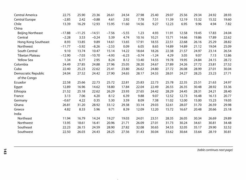
143
Central America 22.75 25.90 23.36 26.61 24.54 27.98 25.40 29.07 25.56 29.34 24.92 28.93Central Europe –2.85 2.42 –0.88 4.61 2.92 7.78 7.51 11.39 12.19 15.32 15.32 19.60Chile 13.39 16.29 12.93 15.95 11.60 14.56 9.27 12.23 6.95 9.96 4.94 7.82China
Beijing Northeast –17.88 –11.25 –14.51 –7.56 –5.55 1.23 4.93 11.91 12.58 19.45 17.83 24.04Central –2.28 3.53 –0.24 5.39 4.74 10.16 10.21 15.71 14.66 19.86 17.89 22.62Hong Kong Southeast 8.93 13.85 9.89 14.61 13.65 17.91 18.55 22.51 22.68 26.16 25.29 28.82Northwest –11.77 –5.92 –8.26 –2.53 0.09 6.05 8.65 14.89 14.89 21.12 19.04 25.09South Central 9.10 13.74 10.47 15.14 14.22 18.64 18.26 22.38 21.57 24.97 23.14 26.54Tibetan Plateau –12.90 –7.03 –10.70 –4.93 –6.23 –0.74 –1.24 4.29 3.05 9.07 7.13 12.86Yellow Sea 1.34 6.77 2.95 8.24 8.12 13.40 14.55 19.78 19.95 24.84 24.15 28.72
Colombia 24.49 27.85 24.88 27.96 25.05 28.20 24.67 27.89 24.26 27.72 23.81 27.52Cuba 22.40 25.23 22.62 25.41 23.80 26.62 24.80 27.72 26.08 28.99 27.01 30.04Democratic Republic 24.04 27.52 24.42 27.90 24.65 28.17 24.55 28.01 24.27 28.25 23.23 27.71
of the CongoEcuador 22.58 25.66 22.73 25.72 22.81 25.83 22.73 25.78 22.35 25.51 21.63 24.97Egypt 12.89 16.96 14.62 18.80 17.84 22.04 22.49 26.55 26.35 30.48 28.92 33.36Ethiopia 21.52 25.18 22.62 26.29 23.93 27.65 24.42 28.29 24.45 28.31 24.21 28.40France 3.13 7.06 4.20 8.12 6.39 9.88 9.07 12.52 12.73 16.48 16.13 20.77Germany –0.67 4.22 0.35 5.30 3.59 8.09 7.38 11.02 12.00 15.00 15.23 19.05Ghana 26.81 31.20 28.92 33.12 29.38 33.14 29.03 32.61 28.07 31.70 26.59 29.98Greece 4.82 8.33 5.96 9.71 8.39 12.09 12.20 15.72 16.67 20.48 20.66 25.18India
Northeast 11.94 16.79 14.24 19.27 19.03 24.01 23.51 28.35 26.05 30.34 26.69 29.89Northwest 13.95 18.61 16.41 20.96 21.71 26.09 27.01 31.73 30.24 34.61 30.81 34.48Southeast 22.23 26.15 24.59 28.90 27.82 32.08 30.65 34.53 32.05 35.17 29.90 32.52Southwest 22.50 26.03 24.43 28.25 27.56 31.43 30.04 33.62 30.64 33.64 28.19 30.81
(table continues next page)
02--Appendices--99-168 6/21/07 11:40 AM Page 143
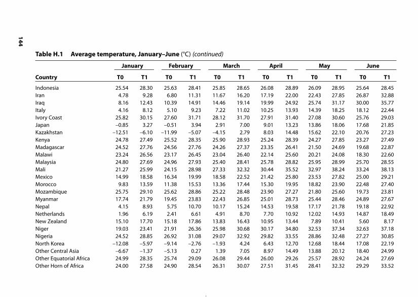
144
Indonesia 25.54 28.30 25.63 28.41 25.85 28.65 26.08 28.89 26.09 28.95 25.64 28.45Iran 4.78 9.28 6.80 11.31 11.67 16.20 17.19 22.00 22.43 27.85 26.87 32.88Iraq 8.16 12.43 10.39 14.91 14.46 19.14 19.99 24.92 25.74 31.17 30.00 35.77Italy 4.16 8.12 5.10 9.23 7.22 11.02 10.25 13.93 14.39 18.25 18.12 22.44Ivory Coast 25.82 30.15 27.60 31.71 28.12 31.70 27.91 31.40 27.08 30.60 25.76 29.03Japan –0.85 3.27 –0.51 3.94 2.91 7.00 9.01 13.23 13.86 18.06 17.68 21.85Kazakhstan –12.51 –6.10 –11.99 –5.07 –4.15 2.79 8.03 14.48 15.62 22.10 20.76 27.23Kenya 24.78 27.49 25.52 28.35 25.90 28.93 25.24 28.39 24.27 27.85 23.27 27.49Madagascar 24.52 27.76 24.56 27.76 24.26 27.37 23.35 26.41 21.50 24.69 19.68 22.87Malawi 23.24 26.56 23.17 26.45 23.04 26.40 22.14 25.60 20.21 24.08 18.30 22.60Malaysia 24.80 27.69 24.96 27.93 25.40 28.41 25.78 28.82 25.95 28.99 25.70 28.55Mali 21.27 25.99 24.15 28.98 27.33 32.32 30.44 35.52 32.97 38.24 33.24 38.13Mexico 14.99 18.58 16.34 19.99 18.58 22.52 21.42 25.80 23.53 27.82 25.00 29.21Morocco 9.83 13.59 11.38 15.53 13.36 17.44 15.30 19.95 18.82 23.90 22.48 27.40Mozambique 25.75 29.10 25.62 28.86 25.22 28.48 23.90 27.27 21.80 25.60 19.73 23.81Myanmar 17.74 21.79 19.45 23.83 22.43 26.85 25.01 28.73 25.44 28.46 24.89 27.67Nepal 4.15 8.93 5.75 10.70 10.17 15.24 14.53 19.58 17.17 21.78 19.18 22.92Netherlands 1.96 6.19 2.41 6.61 4.91 8.70 7.70 10.92 12.02 14.93 14.87 18.49New Zealand 15.10 17.70 15.18 17.86 13.83 16.43 10.95 13.44 7.89 10.41 5.60 8.17Niger 19.03 23.41 21.91 26.36 25.98 30.68 30.17 34.80 32.53 37.34 32.63 37.18Nigeria 24.52 28.85 26.92 31.08 29.07 32.92 29.82 33.55 28.86 32.48 27.27 30.85North Korea –12.08 –5.97 –9.14 –2.76 –1.93 4.24 6.43 12.70 12.68 18.44 17.08 22.19Other Central Asia –6.67 –1.37 –5.13 0.27 1.39 7.05 8.97 14.49 13.88 20.12 18.40 24.99Other Equatorial Africa 24.99 28.35 25.74 29.09 26.08 29.44 26.00 29.26 25.57 28.92 24.24 27.69Other Horn of Africa 24.00 27.58 24.90 28.54 26.31 30.07 27.51 31.45 28.41 32.32 29.29 33.52
Table H.1 Average temperature, January–June (°C) (continued)
January February March April May June
Country T0 T1 T0 T1 T0 T1 T0 T1 T0 T1 T0 T1
02--Appendices--99-168 6/21/07 11:40 AM Page 144
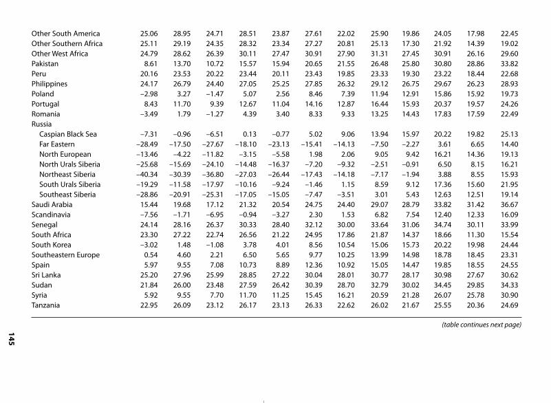
145
Other South America 25.06 28.95 24.71 28.51 23.87 27.61 22.02 25.90 19.86 24.05 17.98 22.45Other Southern Africa 25.11 29.19 24.35 28.32 23.34 27.27 20.81 25.13 17.30 21.92 14.39 19.02Other West Africa 24.79 28.62 26.39 30.11 27.47 30.91 27.90 31.31 27.45 30.91 26.16 29.60Pakistan 8.61 13.70 10.72 15.57 15.94 20.65 21.55 26.48 25.80 30.80 28.86 33.82Peru 20.16 23.53 20.22 23.44 20.11 23.43 19.85 23.33 19.30 23.22 18.44 22.68Philippines 24.17 26.79 24.40 27.05 25.25 27.85 26.32 29.12 26.75 29.67 26.23 28.93Poland –2.98 3.27 –1.47 5.07 2.56 8.46 7.39 11.94 12.91 15.86 15.92 19.73Portugal 8.43 11.70 9.39 12.67 11.04 14.16 12.87 16.44 15.93 20.37 19.57 24.26Romania –3.49 1.79 –1.27 4.39 3.40 8.33 9.33 13.25 14.43 17.83 17.59 22.49Russia
Caspian Black Sea –7.31 –0.96 –6.51 0.13 –0.77 5.02 9.06 13.94 15.97 20.22 19.82 25.13Far Eastern –28.49 –17.50 –27.67 –18.10 –23.13 –15.41 –14.13 –7.50 –2.27 3.61 6.65 14.40North European –13.46 –4.22 –11.82 –3.15 –5.58 1.98 2.06 9.05 9.42 16.21 14.36 19.13North Urals Siberia –25.68 –15.69 –24.10 –14.48 –16.37 –7.20 –9.32 –2.51 –0.91 6.50 8.15 16.21Northeast Siberia –40.34 –30.39 –36.80 –27.03 –26.44 –17.43 –14.18 –7.17 –1.94 3.88 8.55 15.93South Urals Siberia –19.29 –11.58 –17.97 –10.16 –9.24 –1.46 1.15 8.59 9.12 17.36 15.60 21.95Southeast Siberia –28.86 –20.91 –25.31 –17.05 –15.05 –7.47 –3.51 3.01 5.43 12.63 12.51 19.14
Saudi Arabia 15.44 19.68 17.12 21.32 20.54 24.75 24.40 29.07 28.79 33.82 31.42 36.67Scandinavia –7.56 –1.71 –6.95 –0.94 –3.27 2.30 1.53 6.82 7.54 12.40 12.33 16.09Senegal 24.14 28.16 26.37 30.33 28.40 32.12 30.00 33.64 31.06 34.74 30.11 33.99South Africa 23.30 27.22 22.74 26.56 21.22 24.95 17.86 21.87 14.37 18.66 11.30 15.54South Korea –3.02 1.48 –1.08 3.78 4.01 8.56 10.54 15.06 15.73 20.22 19.98 24.44Southeastern Europe 0.54 4.60 2.21 6.50 5.65 9.77 10.25 13.99 14.98 18.78 18.45 23.31Spain 5.97 9.55 7.08 10.73 8.89 12.36 10.92 15.05 14.47 19.85 18.55 24.55Sri Lanka 25.20 27.96 25.99 28.85 27.22 30.04 28.01 30.77 28.17 30.98 27.67 30.62Sudan 21.84 26.00 23.48 27.59 26.42 30.39 28.70 32.79 30.02 34.45 29.85 34.33Syria 5.92 9.55 7.70 11.70 11.25 15.45 16.21 20.59 21.28 26.07 25.78 30.90Tanzania 22.95 26.09 23.12 26.17 23.13 26.33 22.62 26.02 21.67 25.55 20.36 24.69
(table continues next page)
02--Appendices--99-168 6/21/07 11:40 AM Page 145

146
Thailand 23.14 26.98 25.19 28.92 27.27 31.06 28.80 32.12 28.27 31.34 27.46 30.32Turkey 0.09 3.79 1.57 5.71 5.30 9.31 10.48 14.52 14.95 19.60 18.98 24.35Uganda 22.82 25.85 23.31 26.45 23.39 26.81 22.80 26.11 22.30 25.90 21.77 26.03Ukraine –5.21 1.30 –3.80 3.16 1.06 6.97 9.02 13.59 15.09 18.43 18.46 22.96United Kingdom 3.18 6.51 3.21 6.48 4.87 7.88 6.93 9.72 9.96 12.61 12.88 15.79United States
Alaska –19.13 –10.59 –18.32 –11.33 –14.19 –7.15 –7.14 –1.36 2.14 7.87 8.24 13.24Lakes and Northeast –6.96 –0.58 –4.99 1.83 1.20 7.28 8.09 14.25 14.27 19.52 19.25 24.67Pacific Northwest –2.00 2.22 0.64 4.64 3.04 6.63 6.21 9.80 10.35 14.06 14.56 19.58Rockies and Plains –7.69 –2.07 –4.72 1.15 –0.08 5.34 6.29 11.71 12.09 17.20 17.27 23.04Southeast 5.52 9.79 7.52 12.17 12.21 16.50 16.79 21.41 20.93 25.80 24.73 29.75South Pacific Coast 3.08 7.37 5.36 9.18 7.01 10.50 10.00 13.78 14.47 18.72 18.93 23.86Southwest Plains 3.61 8.16 6.17 10.64 9.99 14.33 14.76 19.87 19.23 24.86 23.72 29.54
Uzbekistan –3.29 1.87 –1.87 3.43 5.10 10.61 13.92 19.30 20.35 26.53 25.28 31.76Venezuela 25.14 28.70 25.68 28.85 26.27 29.54 26.22 29.64 25.72 29.37 24.94 28.80Vietnam 19.60 23.52 20.83 24.61 22.42 26.11 25.42 28.87 26.77 30.07 26.96 30.16Yemen 18.96 23.01 19.86 23.87 21.48 25.47 24.14 28.51 26.47 30.71 28.33 32.77Zambia 22.90 26.44 22.91 26.41 22.87 26.41 21.89 25.67 19.61 23.79 17.40 21.97Zimbabwe 23.97 27.60 23.55 27.07 22.93 26.43 21.13 24.91 18.38 22.65 15.75 20.31
T0 = temperature for 1961–90T1 = temperature for 2070–99
Table H.1 Average temperature, January–June (°C) (continued)
January February March April May June
Country T0 T1 T0 T1 T0 T1 T0 T1 T0 T1 T0 T1
02--Appendices--99-168 6/21/07 11:40 AM Page 146
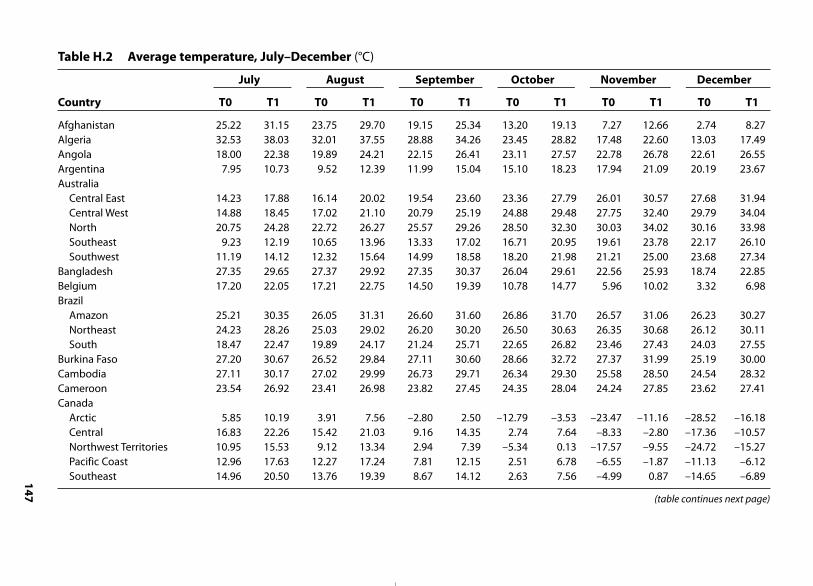
147
Table H.2 Average temperature, July–December (°C)
July August September October November December
Country T0 T1 T0 T1 T0 T1 T0 T1 T0 T1 T0 T1
Afghanistan 25.22 31.15 23.75 29.70 19.15 25.34 13.20 19.13 7.27 12.66 2.74 8.27Algeria 32.53 38.03 32.01 37.55 28.88 34.26 23.45 28.82 17.48 22.60 13.03 17.49Angola 18.00 22.38 19.89 24.21 22.15 26.41 23.11 27.57 22.78 26.78 22.61 26.55Argentina 7.95 10.73 9.52 12.39 11.99 15.04 15.10 18.23 17.94 21.09 20.19 23.67Australia
Central East 14.23 17.88 16.14 20.02 19.54 23.60 23.36 27.79 26.01 30.57 27.68 31.94Central West 14.88 18.45 17.02 21.10 20.79 25.19 24.88 29.48 27.75 32.40 29.79 34.04North 20.75 24.28 22.72 26.27 25.57 29.26 28.50 32.30 30.03 34.02 30.16 33.98Southeast 9.23 12.19 10.65 13.96 13.33 17.02 16.71 20.95 19.61 23.78 22.17 26.10Southwest 11.19 14.12 12.32 15.64 14.99 18.58 18.20 21.98 21.21 25.00 23.68 27.34
Bangladesh 27.35 29.65 27.37 29.92 27.35 30.37 26.04 29.61 22.56 25.93 18.74 22.85Belgium 17.20 22.05 17.21 22.75 14.50 19.39 10.78 14.77 5.96 10.02 3.32 6.98Brazil
Amazon 25.21 30.35 26.05 31.31 26.60 31.60 26.86 31.70 26.57 31.06 26.23 30.27Northeast 24.23 28.26 25.03 29.02 26.20 30.20 26.50 30.63 26.35 30.68 26.12 30.11South 18.47 22.47 19.89 24.17 21.24 25.71 22.65 26.82 23.46 27.43 24.03 27.55
Burkina Faso 27.20 30.67 26.52 29.84 27.11 30.60 28.66 32.72 27.37 31.99 25.19 30.00Cambodia 27.11 30.17 27.02 29.99 26.73 29.71 26.34 29.30 25.58 28.50 24.54 28.32Cameroon 23.54 26.92 23.41 26.98 23.82 27.45 24.35 28.04 24.24 27.85 23.62 27.41Canada
Arctic 5.85 10.19 3.91 7.56 –2.80 2.50 –12.79 –3.53 –23.47 –11.16 –28.52 –16.18Central 16.83 22.26 15.42 21.03 9.16 14.35 2.74 7.64 –8.33 –2.80 –17.36 –10.57Northwest Territories 10.95 15.53 9.12 13.34 2.94 7.39 –5.34 0.13 –17.57 –9.55 –24.72 –15.27Pacific Coast 12.96 17.63 12.27 17.24 7.81 12.15 2.51 6.78 –6.55 –1.87 –11.13 –6.12Southeast 14.96 20.50 13.76 19.39 8.67 14.12 2.63 7.56 –4.99 0.87 –14.65 –6.89
(table continues next page)
02--Appendices--99-168 6/21/07 11:40 AM Page 147

148
Central America 24.76 28.72 24.72 28.32 24.51 27.92 24.09 27.51 23.32 26.72 22.85 26.09Central Europe 17.08 22.65 16.74 23.37 13.50 19.38 8.69 13.27 2.96 7.49 –1.16 3.25Chile 4.63 7.47 5.42 8.36 6.90 9.77 8.82 11.63 10.81 13.54 12.52 15.39China
Beijing Northeast 20.71 25.93 19.12 24.38 12.74 17.99 4.43 9.14 –6.50 –0.47 –15.09 –8.07Central 20.16 24.27 19.63 23.74 15.31 19.66 10.32 14.57 4.20 8.91 –0.74 5.36Hong Kong Southeast 27.69 30.86 27.26 30.64 24.79 28.49 20.47 23.93 15.44 18.72 10.76 15.54Northwest 21.14 27.13 19.97 26.38 14.38 20.42 6.67 11.86 –2.42 3.74 –9.64 –3.30South Central 24.17 27.33 23.76 26.97 21.96 25.50 18.58 22.00 14.24 17.31 10.46 14.70Tibetan Plateau 9.32 14.58 8.74 13.76 5.49 10.47 –0.89 4.45 –7.63 –1.43 –11.50 –5.59Yellow Sea 26.90 30.66 26.38 30.39 21.65 25.91 16.06 19.84 9.50 13.31 3.47 9.08
Colombia 23.68 27.51 23.93 27.83 24.13 27.83 24.21 27.81 24.32 27.83 24.28 27.80Cuba 27.52 30.50 27.53 30.47 27.13 30.12 26.22 29.28 24.69 27.81 23.18 26.14Democratic Republic 22.75 27.31 23.41 27.90 23.99 28.31 24.17 28.63 24.04 27.84 23.91 27.59
of the CongoEcuador 21.18 24.57 21.47 24.84 21.79 25.12 22.02 25.33 22.13 25.40 22.35 25.57Egypt 29.21 34.76 29.20 35.03 27.41 32.55 24.12 28.98 18.60 23.28 14.32 18.71Ethiopia 23.28 27.34 23.04 26.93 23.38 27.31 22.92 26.88 21.95 25.58 21.28 24.85France 18.62 24.42 18.26 24.64 15.81 21.33 11.77 16.00 6.71 10.79 3.89 7.45Germany 16.94 21.76 16.71 22.34 13.63 18.77 9.21 13.41 4.03 8.49 0.69 4.99Ghana 25.57 28.79 25.31 28.57 25.77 29.03 26.76 30.33 27.19 31.29 26.39 30.71Greece 23.13 28.32 22.94 28.24 19.81 24.58 14.85 18.90 10.41 13.98 6.51 10.04India
Northeast 25.14 27.68 24.62 27.38 23.97 27.32 21.44 25.37 16.92 20.77 12.96 17.33Northwest 28.46 31.39 27.24 30.00 26.85 30.05 24.75 28.67 19.79 23.93 15.33 19.75
Table H.2 Average temperature, July–December (°C) (continued)
July August September October November December
Country T0 T1 T0 T1 T0 T1 T0 T1 T0 T1 T0 T1
02--Appendices--99-168 6/21/07 11:40 AM Page 148

149
Southeast 27.51 29.93 27.01 29.39 27.24 30.03 26.34 29.51 23.88 27.09 21.94 25.42Southwest 26.26 28.77 25.72 28.16 26.14 28.74 26.28 29.07 24.36 27.42 22.64 25.91
Indonesia 25.32 28.13 25.44 28.30 25.71 28.54 26.01 28.90 26.02 28.88 25.79 28.60Iran 28.88 35.22 27.56 33.81 23.80 30.07 18.15 23.93 12.07 17.32 6.93 11.68Iraq 32.57 38.79 32.13 38.28 28.71 34.99 22.87 28.46 15.45 20.76 9.87 14.29Italy 20.90 26.21 20.76 26.58 17.88 22.94 13.55 17.77 8.80 12.75 5.26 9.02Ivory Coast 24.77 27.91 24.65 27.85 25.18 28.32 25.82 29.21 26.18 30.03 25.35 29.54Japan 21.68 25.67 23.13 27.21 19.14 23.30 13.13 17.19 7.43 11.49 2.12 6.21Kazakhstan 23.20 30.08 20.69 27.54 14.82 20.60 5.97 11.14 –2.08 3.93 –8.82 –2.38Kenya 22.70 27.06 22.98 26.96 23.79 27.54 24.64 28.41 24.42 27.92 24.44 27.56Madagascar 19.21 22.44 19.59 22.84 20.77 24.02 22.31 25.78 23.47 26.90 24.19 27.52Malawi 17.99 22.45 19.36 23.55 21.78 25.74 24.00 28.62 24.47 29.21 23.75 27.36Malaysia 25.44 28.26 25.41 28.33 25.39 28.29 25.30 28.22 25.07 27.92 24.96 27.81Mali 31.70 36.16 30.56 34.70 30.51 34.72 29.46 34.25 25.57 30.63 21.65 26.50Mexico 24.95 28.98 24.75 28.79 23.63 27.85 21.21 25.55 17.96 22.04 15.60 19.38Morocco 26.28 30.90 26.06 30.44 23.01 27.84 18.42 23.14 13.89 18.48 10.32 14.28Mozambique 19.37 23.58 20.77 24.81 22.91 26.91 24.79 29.35 25.64 30.28 25.72 29.29Myanmar 24.67 27.36 24.59 27.33 24.60 27.59 23.73 26.92 21.15 24.24 18.34 22.14Nepal 19.13 22.17 18.71 21.83 17.50 21.19 13.79 18.10 9.17 13.19 5.56 9.98Netherlands 16.68 20.97 16.79 21.66 14.12 18.65 10.51 14.37 5.89 9.96 3.24 7.02New Zealand 4.92 7.49 6.04 8.44 7.89 10.27 9.87 12.16 11.75 14.07 13.64 16.09Niger 31.05 35.02 30.18 33.79 30.18 34.13 28.33 32.88 23.59 28.13 20.01 24.66Nigeria 25.82 29.04 25.33 28.38 25.91 29.19 26.71 30.38 25.86 29.91 24.61 28.87North Korea 20.71 25.20 20.69 25.25 14.84 19.57 7.98 12.22 –0.61 4.13 –8.81 –2.86Other Central Asia 21.12 27.73 19.81 26.59 14.87 21.23 7.99 13.38 1.52 7.24 –3.76 2.04Other Equatorial Africa 23.29 26.82 23.48 27.24 24.21 27.90 24.67 28.36 24.65 28.04 24.49 27.90Other Horn of Africa 29.02 33.03 28.84 32.66 28.55 32.32 26.72 30.53 25.07 28.67 24.07 27.50Other South America 18.10 22.49 19.82 24.47 21.76 26.52 23.52 27.97 24.41 28.63 24.94 28.96
(table continues next page)
02--Appendices--99-168 6/21/07 11:40 AM Page 149

150
Other Southern Africa 14.24 18.75 16.57 21.12 20.28 24.88 22.91 27.83 24.13 28.66 24.81 29.10Other West Africa 25.00 28.23 24.69 27.80 25.18 28.24 25.74 28.96 25.73 29.22 24.46 28.19Pakistan 28.57 32.94 27.49 31.79 25.15 29.90 20.77 25.94 15.19 20.16 10.30 15.32Peru 18.10 22.48 18.73 23.11 19.35 23.40 19.78 23.63 20.12 23.94 20.14 23.87Philippines 25.87 28.59 25.83 28.59 25.79 28.54 25.58 28.40 25.24 27.97 24.67 27.37Poland 17.47 22.07 17.10 22.58 13.36 18.45 8.72 13.23 3.33 8.43 –0.68 4.59Portugal 22.49 27.17 22.46 26.94 20.39 24.73 16.32 20.20 11.56 15.24 8.73 11.98Romania 19.22 25.97 18.85 26.37 15.20 21.46 9.77 14.70 4.16 8.57 –0.78 3.65Russia
Caspian Black Sea 22.00 28.42 20.81 27.22 15.45 21.02 7.87 13.09 1.55 7.02 –3.69 2.04Far Eastern 10.06 14.98 8.31 13.06 2.49 7.99 –9.14 –1.28 –21.87 –11.09 –27.54 –15.47North European 16.98 21.54 14.77 19.64 9.36 14.07 2.46 7.87 –4.17 2.66 –9.77 –1.60North Urals Siberia 13.46 18.59 10.51 15.83 4.50 10.21 –5.94 1.61 –16.62 –6.03 –22.04 –11.16Northeast Siberia 13.43 17.89 9.50 14.68 1.60 7.56 –12.98 –4.28 –30.95 –18.69 –37.15 –25.11South Urals Siberia 18.21 24.07 15.17 21.55 9.38 14.87 0.29 6.05 –9.14 –1.56 –16.29 –8.26Southeast Siberia 15.81 21.23 13.48 19.54 6.65 12.36 –3.93 1.97 –17.65 –8.91 –26.55 –17.86
Saudi Arabia 31.89 36.94 31.91 36.41 30.07 35.00 25.78 30.87 20.79 25.75 16.75 21.29Scandinavia 14.20 17.87 13.06 17.04 8.89 13.00 4.20 8.42 –1.43 3.58 –5.42 0.20Senegal 28.40 31.95 27.61 30.86 27.75 31.03 28.60 32.18 26.99 30.97 24.14 28.15South Africa 11.20 15.31 13.11 17.39 16.16 20.63 18.47 23.18 20.60 24.97 22.30 26.37South Korea 23.51 27.53 24.18 28.23 19.24 23.44 13.20 17.17 6.20 10.01 –0.15 4.08Southeastern Europe 20.76 27.03 20.55 27.07 17.11 22.65 11.98 16.48 6.78 10.60 2.48 6.27Spain 22.02 28.21 21.82 27.89 19.11 24.48 14.32 18.82 9.34 13.46 6.42 9.89Sri Lanka 27.33 30.29 27.14 30.03 27.07 29.99 26.58 29.42 25.88 28.61 25.32 28.06
Table H.2 Average temperature, July–December (°C) (continued)
July August September October November December
Country T0 T1 T0 T1 T0 T1 T0 T1 T0 T1 T0 T1
02--Appendices--99-168 6/21/07 11:40 AM Page 150
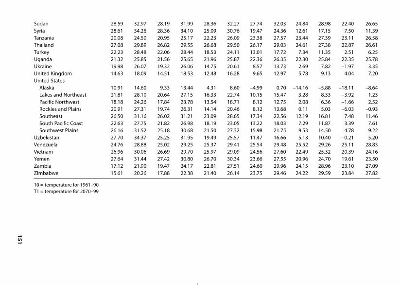
151
Sudan 28.59 32.97 28.19 31.99 28.36 32.27 27.74 32.03 24.84 28.98 22.40 26.65Syria 28.61 34.26 28.36 34.10 25.09 30.76 19.47 24.36 12.61 17.15 7.50 11.39Tanzania 20.08 24.50 20.95 25.17 22.23 26.09 23.38 27.57 23.44 27.39 23.11 26.58Thailand 27.08 29.89 26.82 29.55 26.68 29.50 26.17 29.03 24.61 27.38 22.87 26.61Turkey 22.23 28.48 22.06 28.44 18.53 24.11 13.01 17.72 7.34 11.35 2.51 6.25Uganda 21.32 25.85 21.56 25.65 21.96 25.87 22.36 26.35 22.30 25.84 22.35 25.78Ukraine 19.98 26.07 19.32 26.06 14.75 20.61 8.57 13.73 2.69 7.82 –1.97 3.35United Kingdom 14.63 18.09 14.51 18.53 12.48 16.28 9.65 12.97 5.78 9.13 4.04 7.20United States
Alaska 10.91 14.60 9.33 13.44 4.31 8.60 –4.99 0.70 –14.16 –5.88 –18.11 –8.64Lakes and Northeast 21.81 28.10 20.64 27.15 16.33 22.74 10.15 15.47 3.28 8.33 –3.92 1.23Pacific Northwest 18.18 24.26 17.84 23.78 13.54 18.71 8.12 12.75 2.08 6.36 –1.66 2.52Rockies and Plains 20.91 27.31 19.74 26.31 14.14 20.46 8.12 13.68 0.11 5.03 –6.03 –0.93Southeast 26.50 31.16 26.02 31.21 23.09 28.65 17.34 22.56 12.19 16.81 7.48 11.46South Pacific Coast 22.63 27.75 21.82 26.98 18.19 23.05 13.22 18.03 7.29 11.87 3.39 7.61Southwest Plains 26.16 31.52 25.18 30.68 21.50 27.32 15.98 21.75 9.53 14.50 4.78 9.22
Uzbekistan 27.70 34.37 25.25 31.95 19.49 25.57 11.47 16.66 5.13 10.40 –0.21 5.20Venezuela 24.76 28.88 25.02 29.25 25.37 29.41 25.54 29.48 25.52 29.26 25.11 28.83Vietnam 26.96 30.06 26.69 29.70 25.97 29.09 24.56 27.60 22.49 25.32 20.39 24.16Yemen 27.64 31.44 27.42 30.80 26.70 30.34 23.66 27.55 20.96 24.70 19.61 23.50Zambia 17.12 21.90 19.47 24.17 22.81 27.51 24.60 29.96 24.15 28.96 23.10 27.09Zimbabwe 15.61 20.26 17.88 22.38 21.40 26.14 23.75 29.46 24.22 29.59 23.84 27.82
T0 = temperature for 1961–90T1 = temperature for 2070–99
02--Appendices--99-168 6/21/07 11:40 AM Page 151
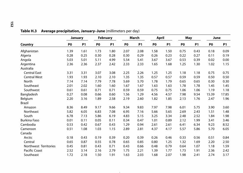
152
Table H.3 Average precipitation, January–June (millimeters per day)
January February March April May June
Country P0 P1 P0 P1 P0 P1 P0 P1 P0 P1 P0 P1
Afghanistan 1.39 1.61 1.73 1.80 2.07 2.08 1.58 1.50 0.75 0.43 0.18 0.09Algeria 0.28 0.25 0.30 0.28 0.30 0.29 0.26 0.23 0.22 0.27 0.11 0.19Angola 5.03 5.01 5.11 4.99 5.54 5.41 3.67 3.67 0.53 0.39 0.02 0.00Argentina 2.36 2.36 2.37 2.42 2.33 2.33 1.65 1.68 1.25 1.30 1.02 1.15Australia
Central East 3.31 3.31 3.07 3.08 2.25 2.26 1.25 1.25 1.18 1.18 0.75 0.75Central West 1.93 1.93 2.10 2.10 1.35 1.35 0.57 0.57 0.59 0.59 0.50 0.50North 7.14 7.14 7.79 7.78 5.69 5.70 1.78 1.79 0.65 0.65 0.30 0.30Southeast 2.01 2.02 1.60 1.60 1.67 1.67 1.63 1.63 1.78 1.78 1.45 1.45Southwest 0.61 0.61 0.71 0.71 0.59 0.59 0.75 0.75 1.06 1.06 1.19 1.18
Bangladesh 0.27 0.08 0.66 0.60 1.56 1.29 4.56 4.57 7.98 9.54 15.39 17.85Belgium 2.20 3.16 1.89 2.58 2.19 2.60 1.82 1.85 2.13 1.76 2.47 1.96Brazil
Amazon 8.36 8.49 9.17 9.66 9.34 9.83 7.97 7.98 6.01 5.75 3.90 3.60Northeast 5.82 6.05 6.83 7.08 6.95 7.16 5.66 5.65 2.69 2.43 1.51 1.48South 6.78 7.13 5.86 6.19 4.83 5.15 3.25 3.34 2.48 2.52 1.84 1.98
Burkina Faso 0.01 0.11 0.05 0.11 0.34 0.47 1.01 0.89 2.12 1.99 3.41 3.46Cambodia 0.53 0.42 0.67 0.43 1.29 0.94 2.61 2.61 6.41 6.34 9.23 8.52Cameroon 0.51 1.08 1.03 1.15 2.89 2.81 4.37 4.17 5.57 5.86 5.70 6.05Canada
Arctic 0.18 0.43 0.19 0.39 0.20 0.39 0.26 0.46 0.33 0.56 0.51 0.84Central 0.65 0.87 0.55 0.78 0.65 0.85 0.80 1.25 1.32 1.69 2.20 2.50Northwest Territories 0.45 0.81 0.43 0.71 0.43 0.66 0.48 0.79 0.64 1.07 1.18 1.59Pacific Coast 2.52 3.14 2.16 2.79 1.75 2.21 1.39 1.77 1.73 1.91 2.36 2.42Southeast 1.72 2.18 1.50 1.91 1.63 2.03 1.68 2.07 1.98 2.41 2.74 3.17
02--Appendices--99-168 6/21/07 11:40 AM Page 152
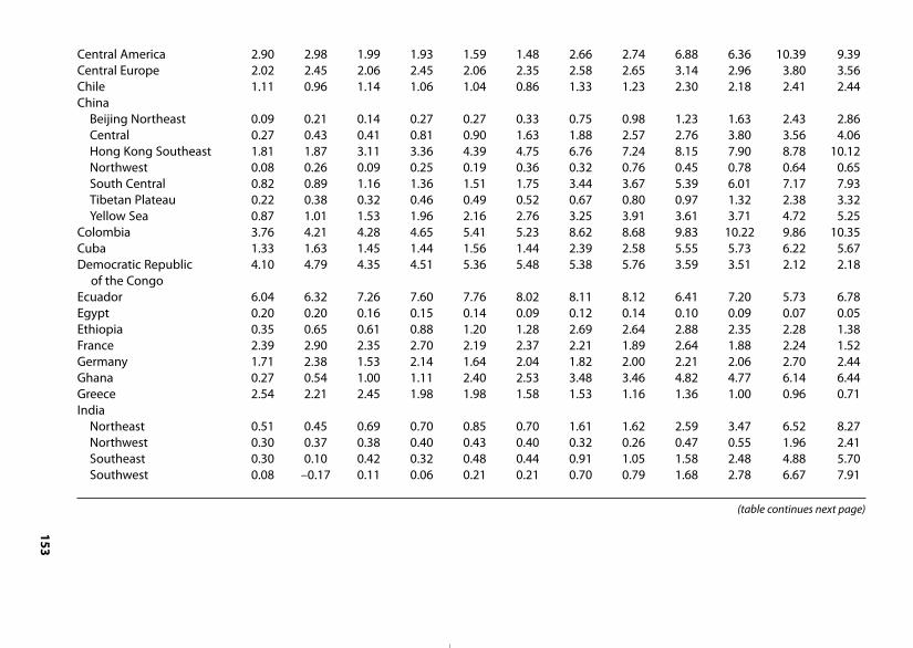
153
Central America 2.90 2.98 1.99 1.93 1.59 1.48 2.66 2.74 6.88 6.36 10.39 9.39Central Europe 2.02 2.45 2.06 2.45 2.06 2.35 2.58 2.65 3.14 2.96 3.80 3.56Chile 1.11 0.96 1.14 1.06 1.04 0.86 1.33 1.23 2.30 2.18 2.41 2.44China
Beijing Northeast 0.09 0.21 0.14 0.27 0.27 0.33 0.75 0.98 1.23 1.63 2.43 2.86Central 0.27 0.43 0.41 0.81 0.90 1.63 1.88 2.57 2.76 3.80 3.56 4.06Hong Kong Southeast 1.81 1.87 3.11 3.36 4.39 4.75 6.76 7.24 8.15 7.90 8.78 10.12Northwest 0.08 0.26 0.09 0.25 0.19 0.36 0.32 0.76 0.45 0.78 0.64 0.65South Central 0.82 0.89 1.16 1.36 1.51 1.75 3.44 3.67 5.39 6.01 7.17 7.93Tibetan Plateau 0.22 0.38 0.32 0.46 0.49 0.52 0.67 0.80 0.97 1.32 2.38 3.32Yellow Sea 0.87 1.01 1.53 1.96 2.16 2.76 3.25 3.91 3.61 3.71 4.72 5.25
Colombia 3.76 4.21 4.28 4.65 5.41 5.23 8.62 8.68 9.83 10.22 9.86 10.35Cuba 1.33 1.63 1.45 1.44 1.56 1.44 2.39 2.58 5.55 5.73 6.22 5.67Democratic Republic 4.10 4.79 4.35 4.51 5.36 5.48 5.38 5.76 3.59 3.51 2.12 2.18
of the CongoEcuador 6.04 6.32 7.26 7.60 7.76 8.02 8.11 8.12 6.41 7.20 5.73 6.78Egypt 0.20 0.20 0.16 0.15 0.14 0.09 0.12 0.14 0.10 0.09 0.07 0.05Ethiopia 0.35 0.65 0.61 0.88 1.20 1.28 2.69 2.64 2.88 2.35 2.28 1.38France 2.39 2.90 2.35 2.70 2.19 2.37 2.21 1.89 2.64 1.88 2.24 1.52Germany 1.71 2.38 1.53 2.14 1.64 2.04 1.82 2.00 2.21 2.06 2.70 2.44Ghana 0.27 0.54 1.00 1.11 2.40 2.53 3.48 3.46 4.82 4.77 6.14 6.44Greece 2.54 2.21 2.45 1.98 1.98 1.58 1.53 1.16 1.36 1.00 0.96 0.71India
Northeast 0.51 0.45 0.69 0.70 0.85 0.70 1.61 1.62 2.59 3.47 6.52 8.27Northwest 0.30 0.37 0.38 0.40 0.43 0.40 0.32 0.26 0.47 0.55 1.96 2.41Southeast 0.30 0.10 0.42 0.32 0.48 0.44 0.91 1.05 1.58 2.48 4.88 5.70Southwest 0.08 –0.17 0.11 0.06 0.21 0.21 0.70 0.79 1.68 2.78 6.67 7.91
(table continues next page)
02--Appendices--99-168 6/21/07 11:40 AM Page 153
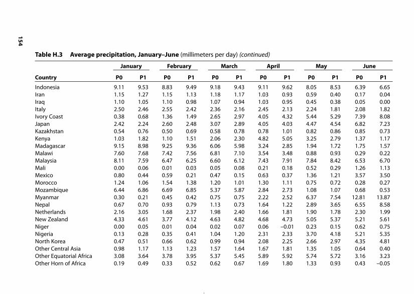
154
Indonesia 9.11 9.53 8.83 9.49 9.18 9.43 9.11 9.62 8.05 8.53 6.39 6.65Iran 1.15 1.27 1.15 1.13 1.18 1.17 1.03 0.93 0.59 0.40 0.17 0.04Iraq 1.10 1.05 1.10 0.98 1.07 0.94 1.03 0.95 0.45 0.38 0.05 0.00Italy 2.50 2.46 2.55 2.42 2.36 2.16 2.45 2.13 2.24 1.81 2.08 1.82Ivory Coast 0.38 0.68 1.36 1.49 2.65 2.97 4.05 4.32 5.44 5.29 7.39 8.08Japan 2.42 2.24 2.60 2.48 3.07 2.89 4.05 4.03 4.47 4.54 6.82 7.23Kazakhstan 0.54 0.76 0.50 0.69 0.58 0.78 0.78 1.01 0.82 0.86 0.85 0.73Kenya 1.03 1.82 1.10 1.51 2.06 2.30 4.82 5.05 3.25 2.79 1.37 1.17Madagascar 9.15 8.98 9.25 9.36 6.06 5.98 3.24 2.85 1.94 1.72 1.75 1.57Malawi 7.60 7.68 7.42 7.56 6.81 7.10 3.54 3.48 0.88 0.93 0.29 0.22Malaysia 8.11 7.59 6.47 6.25 6.60 6.12 7.43 7.91 7.84 8.42 6.53 6.70Mali 0.00 0.06 0.01 0.03 0.05 0.08 0.21 0.18 0.52 0.29 1.26 1.13Mexico 0.80 0.44 0.59 0.21 0.47 0.15 0.63 0.37 1.36 1.21 3.57 3.50Morocco 1.24 1.06 1.54 1.38 1.20 1.01 1.30 1.11 0.75 0.72 0.28 0.27Mozambique 6.44 6.86 6.69 6.85 5.37 5.87 2.84 2.73 1.08 1.07 0.68 0.53Myanmar 0.30 0.21 0.45 0.42 0.75 0.75 2.22 2.52 6.37 7.54 12.81 13.87Nepal 0.67 0.70 0.93 0.79 1.13 0.73 1.64 1.22 2.89 3.65 6.55 8.58Netherlands 2.16 3.05 1.68 2.37 1.98 2.40 1.66 1.81 1.90 1.78 2.30 1.99New Zealand 4.33 4.61 3.77 4.12 4.63 4.82 4.68 4.73 5.05 5.37 5.21 5.61Niger 0.00 0.05 0.01 0.04 0.02 0.07 0.06 –0.01 0.23 0.15 0.62 0.75Nigeria 0.13 0.28 0.35 0.41 1.04 1.20 2.31 2.33 3.70 4.18 5.21 5.35North Korea 0.47 0.51 0.66 0.62 0.99 0.94 2.08 2.25 2.66 2.97 4.35 4.81Other Central Asia 0.98 1.17 1.13 1.23 1.57 1.64 1.67 1.81 1.35 1.05 0.64 0.40Other Equatorial Africa 3.08 3.64 3.78 3.95 5.37 5.45 5.89 5.92 5.74 5.72 3.16 3.23Other Horn of Africa 0.19 0.49 0.33 0.52 0.62 0.67 1.69 1.80 1.33 0.93 0.43 –0.05
Table H.3 Average precipitation, January–June (millimeters per day) (continued)
January February March April May June
Country P0 P1 P0 P1 P0 P1 P0 P1 P0 P1 P0 P1
02--Appendices--99-168 6/21/07 11:40 AM Page 154
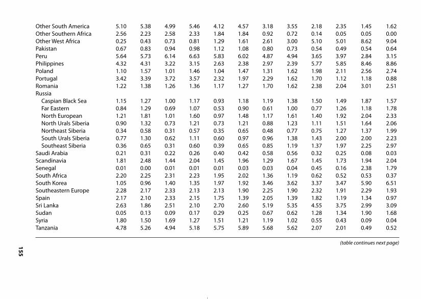
155
Other South America 5.10 5.38 4.99 5.46 4.12 4.57 3.18 3.55 2.18 2.35 1.45 1.62Other Southern Africa 2.56 2.23 2.58 2.33 1.84 1.84 0.92 0.72 0.14 0.05 0.05 0.00Other West Africa 0.25 0.43 0.73 0.81 1.29 1.61 2.61 3.00 5.10 5.01 8.62 9.04Pakistan 0.67 0.83 0.94 0.98 1.12 1.08 0.80 0.73 0.54 0.49 0.54 0.64Peru 5.64 5.73 6.14 6.63 5.83 6.02 4.87 4.94 3.65 3.97 2.84 3.15Philippines 4.32 4.31 3.22 3.15 2.63 2.38 2.97 2.39 5.77 5.85 8.46 8.86Poland 1.10 1.57 1.01 1.46 1.04 1.47 1.31 1.62 1.98 2.11 2.56 2.74Portugal 3.42 3.39 3.72 3.57 2.32 1.97 2.29 1.62 1.70 1.12 1.18 0.88Romania 1.22 1.38 1.26 1.36 1.17 1.27 1.70 1.62 2.38 2.04 3.01 2.51Russia
Caspian Black Sea 1.15 1.27 1.00 1.17 0.93 1.18 1.19 1.38 1.50 1.49 1.87 1.57Far Eastern 0.84 1.29 0.69 1.07 0.53 0.90 0.61 1.00 0.77 1.26 1.18 1.78North European 1.21 1.81 1.01 1.60 0.97 1.48 1.17 1.61 1.40 1.92 2.04 2.33North Urals Siberia 0.90 1.32 0.73 1.21 0.73 1.21 0.88 1.23 1.11 1.51 1.64 2.06Northeast Siberia 0.34 0.58 0.31 0.57 0.35 0.65 0.48 0.77 0.75 1.27 1.37 1.99South Urals Siberia 0.77 1.30 0.62 1.11 0.60 0.97 0.96 1.38 1.43 2.00 2.00 2.23Southeast Siberia 0.36 0.65 0.31 0.60 0.39 0.65 0.85 1.19 1.37 1.97 2.25 2.97
Saudi Arabia 0.21 0.31 0.22 0.26 0.40 0.42 0.58 0.56 0.32 0.25 0.08 0.03Scandinavia 1.81 2.48 1.44 2.04 1.45 1.96 1.29 1.67 1.45 1.73 1.94 2.04Senegal 0.01 0.00 0.01 0.01 0.01 0.03 0.03 0.04 0.45 0.16 2.38 1.79South Africa 2.20 2.25 2.31 2.23 1.95 2.02 1.36 1.19 0.62 0.52 0.53 0.37South Korea 1.05 0.96 1.40 1.35 1.97 1.92 3.46 3.62 3.37 3.47 5.90 6.51Southeastern Europe 2.28 2.17 2.33 2.13 2.13 1.90 2.25 1.90 2.32 1.91 2.29 1.93Spain 2.17 2.10 2.33 2.15 1.75 1.39 2.05 1.39 1.82 1.19 1.34 0.97Sri Lanka 2.63 1.86 2.51 2.10 2.70 2.60 5.19 5.35 4.55 3.75 2.99 3.09Sudan 0.05 0.13 0.09 0.17 0.29 0.25 0.67 0.62 1.28 1.34 1.90 1.68Syria 1.80 1.50 1.69 1.27 1.51 1.21 1.19 1.02 0.55 0.43 0.09 0.04Tanzania 4.78 5.26 4.94 5.18 5.75 5.89 5.68 5.62 2.07 2.01 0.49 0.52
(table continues next page)
02--Appendices--99-168 6/21/07 11:40 AM Page 155
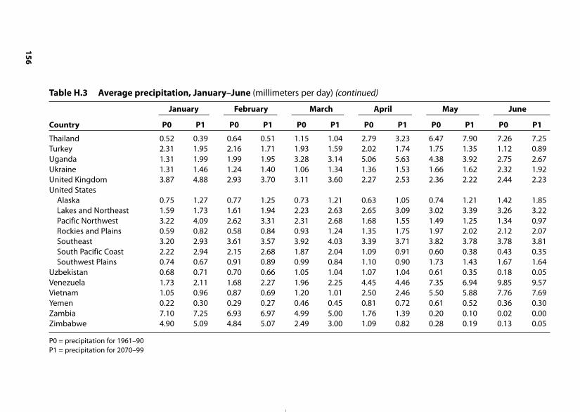
156
Thailand 0.52 0.39 0.64 0.51 1.15 1.04 2.79 3.23 6.47 7.90 7.26 7.25Turkey 2.31 1.95 2.16 1.71 1.93 1.59 2.02 1.74 1.75 1.35 1.12 0.89Uganda 1.31 1.99 1.99 1.95 3.28 3.14 5.06 5.63 4.38 3.92 2.75 2.67Ukraine 1.31 1.46 1.24 1.40 1.06 1.34 1.36 1.53 1.66 1.62 2.32 1.92United Kingdom 3.87 4.88 2.93 3.70 3.11 3.60 2.27 2.53 2.36 2.22 2.44 2.23United States
Alaska 0.75 1.27 0.77 1.25 0.73 1.21 0.63 1.05 0.74 1.21 1.42 1.85Lakes and Northeast 1.59 1.73 1.61 1.94 2.23 2.63 2.65 3.09 3.02 3.39 3.26 3.22Pacific Northwest 3.22 4.09 2.62 3.31 2.31 2.68 1.68 1.55 1.49 1.25 1.34 0.97Rockies and Plains 0.59 0.82 0.58 0.84 0.93 1.24 1.35 1.75 1.97 2.02 2.12 2.07Southeast 3.20 2.93 3.61 3.57 3.92 4.03 3.39 3.71 3.82 3.78 3.78 3.81South Pacific Coast 2.22 2.94 2.15 2.68 1.87 2.04 1.09 0.91 0.60 0.38 0.43 0.35Southwest Plains 0.74 0.67 0.91 0.89 0.99 0.84 1.10 0.90 1.73 1.43 1.67 1.64
Uzbekistan 0.68 0.71 0.70 0.66 1.05 1.04 1.07 1.04 0.61 0.35 0.18 0.05Venezuela 1.73 2.11 1.68 2.27 1.96 2.25 4.45 4.46 7.35 6.94 9.85 9.57Vietnam 1.05 0.96 0.87 0.69 1.20 1.01 2.50 2.46 5.50 5.88 7.76 7.69Yemen 0.22 0.30 0.29 0.27 0.46 0.45 0.81 0.72 0.61 0.52 0.36 0.30Zambia 7.10 7.25 6.93 6.97 4.99 5.00 1.76 1.39 0.20 0.10 0.02 0.00Zimbabwe 4.90 5.09 4.84 5.07 2.49 3.00 1.09 0.82 0.28 0.19 0.13 0.05
P0 = precipitation for 1961–90P1 = precipitation for 2070–99
Table H.3 Average precipitation, January–June (millimeters per day) (continued)
January February March April May June
Country P0 P1 P0 P1 P0 P1 P0 P1 P0 P1 P0 P1
02--Appendices--99-168 6/21/07 11:40 AM Page 156
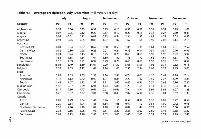
157
Table H.4 Average precipitation, July–December (millimeters per day)
July August September October November December
Country P0 P1 P0 P1 P0 P1 P0 P1 P0 P1 P0 P1
Afghanistan 0.34 0.36 0.33 0.39 0.15 0.16 0.32 0.28 0.51 0.54 0.99 1.08Algeria 0.07 0.05 0.12 0.27 0.17 0.19 0.23 0.18 0.31 0.27 0.30 0.31Angola 0.02 –0.01 0.12 0.09 0.73 0.54 2.36 1.97 4.82 4.58 5.05 4.83Argentina 0.94 0.95 0.85 0.83 1.07 1.02 1.62 1.66 1.95 2.08 2.14 2.18Australia
Central East 0.84 0.84 0.67 0.67 0.60 0.59 1.06 1.05 1.64 1.64 2.51 2.52Central West 0.36 0.36 0.25 0.25 0.21 0.21 0.35 0.34 0.59 0.59 0.96 0.96North 0.24 0.24 0.13 0.13 0.25 0.25 0.68 0.68 1.98 1.98 3.92 3.92Southeast 1.58 1.58 1.64 1.64 1.50 1.49 1.73 1.72 1.62 1.61 1.67 1.67Southwest 1.10 1.09 0.92 0.92 0.79 0.78 0.68 0.68 0.58 0.57 0.52 0.52
Bangladesh 16.93 18.79 13.19 14.07 10.09 11.32 5.08 5.53 1.03 0.71 0.32 0.15Belgium 2.33 1.65 2.12 1.44 2.14 1.60 2.35 2.34 2.65 3.25 2.49 3.03Brazil
Amazon 2.88 2.65 2.55 2.33 3.34 2.91 4.74 4.06 6.10 5.64 7.29 7.14Northeast 1.16 1.12 0.72 0.90 1.01 0.85 2.29 1.92 3.59 2.77 4.79 4.85South 1.64 1.67 1.72 1.57 2.71 2.62 4.41 4.56 5.50 5.92 6.76 7.20
Burkina Faso 5.48 5.57 6.79 6.91 4.74 5.81 1.28 1.65 0.11 0.36 0.04 0.12Cambodia 9.19 9.16 9.97 9.61 10.61 10.66 7.94 8.91 3.94 3.63 1.27 1.28Cameroon 6.28 6.07 7.27 7.04 8.68 8.43 7.02 6.94 2.36 3.04 0.62 1.38Canada
Arctic 0.89 1.29 1.04 1.44 0.76 1.16 0.59 0.99 0.36 0.81 0.22 0.54Central 2.29 2.34 1.94 1.88 1.64 1.66 0.97 1.12 0.81 1.00 0.72 0.98Northwest Territories 1.58 1.90 1.49 1.82 1.10 1.58 0.89 1.44 0.72 1.26 0.50 0.93Pacific Coast 2.36 2.16 2.06 1.93 2.11 2.29 2.35 3.02 2.60 3.46 2.58 3.32Southeast 3.03 3.13 2.98 2.98 3.02 3.05 2.45 2.60 2.34 2.72 1.99 2.42
(table continues next page)
02--Appendices--99-168 6/21/07 11:40 AM Page 157
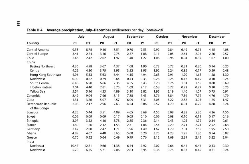
158
Central America 9.53 8.75 9.10 8.51 10.70 9.53 9.92 9.84 6.49 6.71 4.15 4.08Central Europe 3.41 2.74 3.46 2.75 2.57 1.88 2.11 2.05 2.61 2.94 2.26 2.57Chile 2.46 2.42 2.02 1.97 1.40 1.27 1.06 0.96 0.94 0.82 1.07 1.00China
Beijing Northeast 4.36 4.98 3.67 4.37 1.68 1.90 0.73 0.72 0.31 0.30 0.14 0.25Central 4.26 4.50 3.75 3.95 3.52 3.95 1.92 2.24 0.82 0.77 0.29 0.48Hong Kong Southeast 4.96 5.33 5.63 6.44 4.15 4.94 2.68 2.91 1.90 1.68 1.28 1.30Northwest 0.90 0.62 0.79 0.64 0.43 0.33 0.26 0.25 0.17 0.19 0.10 0.24South Central 6.48 6.90 6.66 7.35 4.55 5.43 3.28 3.76 1.81 1.65 0.80 0.69Tibetan Plateau 3.04 4.40 2.81 3.75 1.69 2.12 0.58 0.72 0.22 0.27 0.20 0.25Yellow Sea 5.54 5.96 4.33 4.89 3.10 3.82 1.95 2.19 1.40 1.07 0.75 0.91
Colombia 8.49 9.04 7.96 8.15 7.88 7.45 8.76 8.84 7.36 7.72 4.76 4.79Cuba 4.31 3.86 5.07 4.57 6.09 5.31 5.05 5.22 2.58 3.05 1.25 1.47Democratic Republic 2.08 2.17 2.96 2.63 4.24 3.86 5.52 4.79 6.01 6.25 4.88 5.24
of the CongoEcuador 4.25 5.44 3.51 4.09 4.05 3.69 4.55 5.08 4.28 5.26 4.26 4.56Egypt 0.09 0.09 0.09 0.17 0.05 0.10 0.09 0.08 0.10 0.11 0.17 0.16Ethiopia 3.97 3.52 4.10 3.78 2.85 2.36 2.14 2.43 1.05 1.72 0.34 0.61France 1.80 1.26 2.12 1.53 2.31 1.86 2.54 2.29 2.71 2.74 2.52 2.68Germany 2.42 2.00 2.42 1.71 1.96 1.49 1.67 1.79 2.01 2.55 1.95 2.50Ghana 4.89 4.67 4.48 3.65 5.68 5.20 3.75 4.23 1.25 1.86 0.54 0.82Greece 0.70 0.52 0.64 0.49 0.99 0.76 2.12 1.69 2.89 2.45 3.22 3.04India
Northeast 10.47 12.81 9.66 11.38 6.44 7.92 2.02 2.66 0.44 0.44 0.33 0.30Northwest 5.70 6.75 5.71 7.06 2.83 3.95 0.36 0.75 0.33 0.49 0.21 0.24
Table H.4 Average precipitation, July–December (millimeters per day) (continued)
July August September October November December
Country P0 P1 P0 P1 P0 P1 P0 P1 P0 P1 P0 P1
02--Appendices--99-168 6/21/07 11:40 AM Page 158
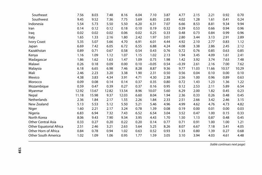
159
Southeast 7.56 8.03 7.48 8.16 6.04 7.10 3.87 4.77 2.15 2.21 0.92 0.70Southwest 9.45 9.52 7.36 7.75 5.69 6.85 2.85 4.02 1.28 1.61 0.41 0.24
Indonesia 5.54 5.73 5.50 5.50 6.20 6.31 7.07 6.66 8.53 8.81 9.34 9.94Iran 0.14 0.12 0.12 0.18 0.10 0.19 0.32 0.39 0.53 0.66 0.94 0.96Iraq 0.02 0.02 0.02 0.06 0.02 0.25 0.33 0.48 0.73 0.84 0.99 0.96Italy 1.65 1.33 2.16 1.80 2.42 1.97 3.01 2.80 3.44 3.13 2.91 2.89Ivory Coast 5.35 5.07 5.66 4.70 6.91 6.01 4.44 4.92 2.10 2.77 0.83 1.12Japan 6.69 7.42 6.05 6.72 6.55 6.88 4.24 4.08 3.38 2.86 2.45 2.12Kazakhstan 0.89 0.71 0.67 0.58 0.54 0.43 0.76 0.72 0.76 0.85 0.63 0.85Kenya 1.16 1.09 1.12 1.07 1.15 1.02 2.13 1.94 3.45 4.09 1.61 2.41Madagascar 1.86 1.62 1.63 1.47 1.09 0.75 1.98 1.42 3.92 3.74 7.63 7.48Malawi 0.26 0.18 0.09 0.00 0.10 –0.05 0.54 –0.39 2.61 2.16 7.00 7.62Malaysia 6.18 6.65 6.98 7.46 8.28 8.87 9.36 9.77 11.03 11.66 10.57 10.29Mali 2.46 2.23 3.20 3.38 1.90 2.31 0.50 0.56 0.04 0.10 0.00 0.10Mexico 4.38 3.83 4.34 3.91 4.71 4.30 2.38 2.56 1.00 0.96 0.89 0.63Morocco 0.09 0.08 0.14 0.14 0.37 0.35 0.80 0.72 1.43 1.23 1.36 1.22Mozambique 0.59 0.47 0.39 0.27 0.37 0.16 0.95 0.12 2.53 2.11 5.89 6.54Myanmar 12.92 13.67 12.82 13.54 8.96 10.07 5.60 6.29 2.00 1.82 0.45 0.23Nepal 11.18 15.98 9.37 12.03 6.60 8.04 1.94 2.36 0.33 0.26 0.48 0.45Netherlands 2.36 1.84 2.17 1.55 2.26 1.84 2.33 2.51 2.66 3.42 2.46 3.15New Zealand 5.13 5.53 5.12 5.50 5.21 5.46 4.96 4.99 4.62 4.76 4.73 4.82Niger 1.60 2.21 2.17 3.24 0.78 1.39 0.08 0.19 0.00 0.01 0.00 0.03Nigeria 6.83 6.94 7.32 7.43 6.52 6.54 3.04 3.52 0.47 1.00 0.15 0.33North Korea 8.06 9.43 7.90 9.34 3.95 4.43 1.70 1.50 1.13 0.87 0.48 0.45Other Central Asia 0.33 0.27 0.20 0.22 0.20 0.14 0.77 0.71 0.91 1.00 1.00 1.21Other Equatorial Africa 2.51 2.46 3.21 2.63 5.64 5.25 8.26 8.07 6.67 7.18 3.41 4.05Other Horn of Africa 0.84 0.78 0.94 1.02 0.63 0.52 0.93 1.33 0.80 1.39 0.27 0.68Other South America 1.02 1.09 1.06 0.95 1.77 1.59 3.05 3.10 3.94 4.03 4.61 4.48
(table continues next page)
02--Appendices--99-168 6/21/07 11:40 AM Page 159
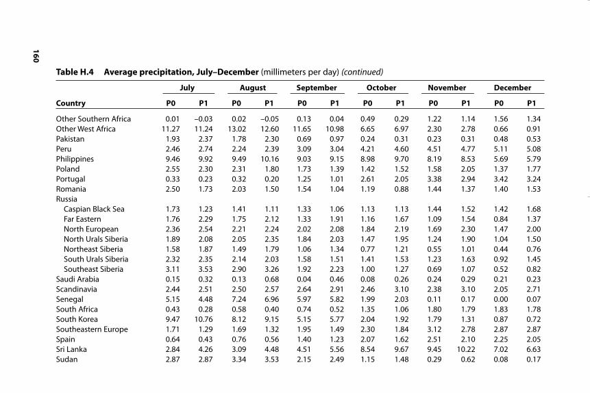
160
Other Southern Africa 0.01 –0.03 0.02 –0.05 0.13 0.04 0.49 0.29 1.22 1.14 1.56 1.34Other West Africa 11.27 11.24 13.02 12.60 11.65 10.98 6.65 6.97 2.30 2.78 0.66 0.91Pakistan 1.93 2.37 1.78 2.30 0.69 0.97 0.24 0.31 0.23 0.31 0.48 0.53Peru 2.46 2.74 2.24 2.39 3.09 3.04 4.21 4.60 4.51 4.77 5.11 5.08Philippines 9.46 9.92 9.49 10.16 9.03 9.15 8.98 9.70 8.19 8.53 5.69 5.79Poland 2.55 2.30 2.31 1.80 1.73 1.39 1.42 1.52 1.58 2.05 1.37 1.77Portugal 0.33 0.23 0.32 0.20 1.25 1.01 2.61 2.05 3.38 2.94 3.42 3.24Romania 2.50 1.73 2.03 1.50 1.54 1.04 1.19 0.88 1.44 1.37 1.40 1.53Russia
Caspian Black Sea 1.73 1.23 1.41 1.11 1.33 1.06 1.13 1.13 1.44 1.52 1.42 1.68Far Eastern 1.76 2.29 1.75 2.12 1.33 1.91 1.16 1.67 1.09 1.54 0.84 1.37North European 2.36 2.54 2.21 2.24 2.02 2.08 1.84 2.19 1.69 2.30 1.47 2.00North Urals Siberia 1.89 2.08 2.05 2.35 1.84 2.03 1.47 1.95 1.24 1.90 1.04 1.50Northeast Siberia 1.58 1.87 1.49 1.79 1.06 1.34 0.77 1.21 0.55 1.01 0.44 0.76South Urals Siberia 2.32 2.35 2.14 2.03 1.58 1.51 1.41 1.53 1.23 1.63 0.92 1.45Southeast Siberia 3.11 3.53 2.90 3.26 1.92 2.23 1.00 1.27 0.69 1.07 0.52 0.82
Saudi Arabia 0.15 0.32 0.13 0.68 0.04 0.46 0.08 0.26 0.24 0.29 0.21 0.23Scandinavia 2.44 2.51 2.50 2.57 2.64 2.91 2.46 3.10 2.38 3.10 2.05 2.71Senegal 5.15 4.48 7.24 6.96 5.97 5.82 1.99 2.03 0.11 0.17 0.00 0.07South Africa 0.43 0.28 0.58 0.40 0.74 0.52 1.35 1.06 1.80 1.79 1.83 1.78South Korea 9.47 10.76 8.12 9.15 5.15 5.77 2.04 1.92 1.79 1.31 0.87 0.72Southeastern Europe 1.71 1.29 1.69 1.32 1.95 1.49 2.30 1.84 3.12 2.78 2.87 2.87Spain 0.64 0.43 0.76 0.56 1.40 1.23 2.07 1.62 2.51 2.10 2.25 2.05Sri Lanka 2.84 4.26 3.09 4.48 4.51 5.56 8.54 9.67 9.45 10.22 7.02 6.63Sudan 2.87 2.87 3.34 3.53 2.15 2.49 1.15 1.48 0.29 0.62 0.08 0.17
Table H.4 Average precipitation, July–December (millimeters per day) (continued)
July August September October November December
Country P0 P1 P0 P1 P0 P1 P0 P1 P0 P1 P0 P1
02--Appendices--99-168 6/21/07 11:40 AM Page 160

161
Syria 0.02 0.00 0.02 0.03 0.05 0.11 0.66 0.61 1.11 0.96 1.74 1.58Tanzania 0.30 0.32 0.32 0.37 0.60 0.47 1.14 0.46 3.41 3.33 5.14 5.53Thailand 7.18 8.05 8.54 8.81 8.82 9.54 5.46 6.23 2.66 2.47 1.02 0.91Turkey 0.50 0.28 0.44 0.25 0.63 0.53 1.42 1.22 1.93 1.66 2.56 2.37Uganda 2.86 3.19 3.63 3.57 3.82 3.13 3.99 3.16 3.95 4.66 1.88 2.57Ukraine 2.31 1.69 1.74 1.35 1.45 1.09 1.09 1.00 1.45 1.49 1.56 1.77United Kingdom 2.40 2.05 2.97 2.58 3.49 3.30 3.78 4.08 3.97 4.71 3.93 4.58United States
Alaska 1.83 2.47 1.96 2.48 1.69 2.29 1.21 1.92 1.00 1.73 0.94 1.66Lakes and Northeast 3.11 2.90 3.09 3.04 3.06 2.80 2.35 2.32 2.40 2.47 2.06 2.10Pacific Northwest 0.66 0.42 0.87 0.71 1.18 0.96 1.75 1.61 3.23 3.49 3.44 4.06Rockies and Plains 1.62 1.27 1.44 1.26 1.35 1.20 0.94 0.94 0.69 0.79 0.62 0.72Southeast 3.94 3.77 3.54 3.31 3.54 3.32 2.71 2.58 3.27 3.15 3.51 3.37South Pacific Coast 0.37 0.35 0.49 0.53 0.57 0.65 0.88 0.85 1.98 2.05 2.03 2.55Southwest Plains 1.73 1.56 1.98 1.74 2.11 1.74 1.44 1.42 0.99 0.84 0.84 0.72
Uzbekistan 0.12 0.07 0.05 0.07 0.09 0.07 0.41 0.34 0.57 0.56 0.72 0.78Venezuela 9.23 8.62 8.44 8.33 6.69 6.30 5.49 5.42 4.40 4.61 2.64 2.85Vietnam 8.05 7.96 8.63 8.78 8.66 9.07 7.10 7.99 5.03 4.83 2.12 2.00Yemen 0.85 1.14 0.78 1.32 0.32 0.82 0.21 0.86 0.30 0.54 0.26 0.40Zambia 0.01 –0.04 0.01 –0.07 0.15 –0.01 1.03 0.08 3.71 3.50 7.13 7.11Zimbabwe 0.07 0.02 0.09 0.00 0.25 0.08 0.86 –0.04 2.51 2.26 4.71 5.25
P0 = precipitation for 1961–90P1 = precipitation for 2070–99
02--Appendices--99-168 6/21/07 11:40 AM Page 161

02--Appendices--99-168 6/21/07 11:40 AM Page 162
Appendix IDispersion of ClimateProjections Across GeneralCirculation Models
It is often argued that climate general circulation models (GCMs) givesuch widely divergent projections at detailed geographical levels that theydo not provide the basis for examining future climate change effects atsuch levels. This appendix examines the degree of dispersion across the sixGCMs used in this study for projected temperature and precipitation by2070–99. The average levels for this period are shown in 4.2 in chapter 4.
This appendix considers the coefficient of variation of these projectionsacross the six climate models listed in table 4.1. This measure, which is theratio of the standard deviation (square root of the sum of square residualsfrom mean) to the mean, is the most natural gauge of dispersion to con-sider. Even so it is inherently problematic for climate measures. It de-pends on the level of the mean, and of course as the mean approacheszero it approaches infinity even if the variation around the mean is small.As usually measured (in Celsius or Fahrenheit), temperature in particularis not a “ratio scale” number with absolute zero but a relative numberwith arbitrary zero. In contrast, temperature measured in kelvin (K) is ina ratio scale. Because it will show a much larger mean value (e.g., 287 Krather than 14°C), the coefficient of variation will be much smaller whencalculated using kelvin than when using Celsius.1
163
1. Moreover, because Celsius is not a ratio scale number it is meaningless to say that post-warming temperatures will be x percent higher than today’s levels. Some of the Ricardian
02--Appendices--99-168 6/21/07 11:40 AM Page 163

Similarly, the coefficient of variation will be quite different if it is calcu-lated for alternative future levels of temperature and precipitation againstfuture means from what would be calculated using instead the change intemperature or change in precipitation from present-day levels. Thechange variables will have much smaller means than the level variables,potentially generating an extreme measure of coefficient of variation.
With these caveats in mind, it is useful to consider the coefficient ofvariation for the projected future levels of temperature and precipitationacross the six GCM projections for 2070–99. These are reported in table I.1.For future temperatures, the coefficient of variation shows a relatively lowmedian of 0.10. That is, for the typical case, the standard deviation acrossthe six models is only 10 percent of the mean value, even though the mea-sure used is Celsius. For precipitation, the median coefficient of variationis 0.33. This extent of dispersion is considerably higher. However, asnoted in the discussion of the estimates using the various Ricardian mod-els (chapter 5), the coefficients in these empirically estimated models tendto show lesser agricultural impact from future changes in precipitationthan from future changes in temperature. Significant variability in theprecipitation projections is unlikely to be particularly problematic for theimpact projections, given the relatively low dispersion in the temperatureprojections.
As expected, the measured dispersion can be large where the level ofthe mean is close to zero (e.g., in Alaska the coefficient of variation for fu-ture temperature is 6.68; it is negative for Arctic Canada because the fu-ture mean temperature is below zero). Aside from such cases, the onlysurprisingly high coefficient of variation for temperature is in the case ofNortheastern India, where it reaches 3.64. Otherwise, it seems fair to saythat the variability of the climate model projections of future temperatureis perhaps surprisingly modest, in light of the seeming reputation of suchmodels for sharp variability.
The same can largely be said about the results for precipitation. Thecases with high coefficients of variation (e.g., above 1) tend to be regionswith low present and future precipitation (e.g., Algeria at 0.23 mm perday, Egypt at 0.12 mm per day, Niger at 0.68 mm per day, and Yemen at0.64 mm per day; future levels in all cases). Once again, however, there areintriguing exceptions. The coefficient of variation for future precipitationis relatively high for Argentina, Brazil’s Northeast, India’s Northwest,Mexico, and the US South Pacific Coast, even though none of these re-gions has a level of future precipitation below 1 mm per day. True vari-ability across the models appears to be present in such cases. Nonetheless,
164 GLOBAL WARMING AND AGRICULTURE
impact studies have slipped into the misnomer of identifying “elasticities” of impact withrespect to temperature—a concept that instead would require a meaningful percentagechange in temperature and hence the use of kelvin.
02--Appendices--99-168 6/21/07 11:40 AM Page 164
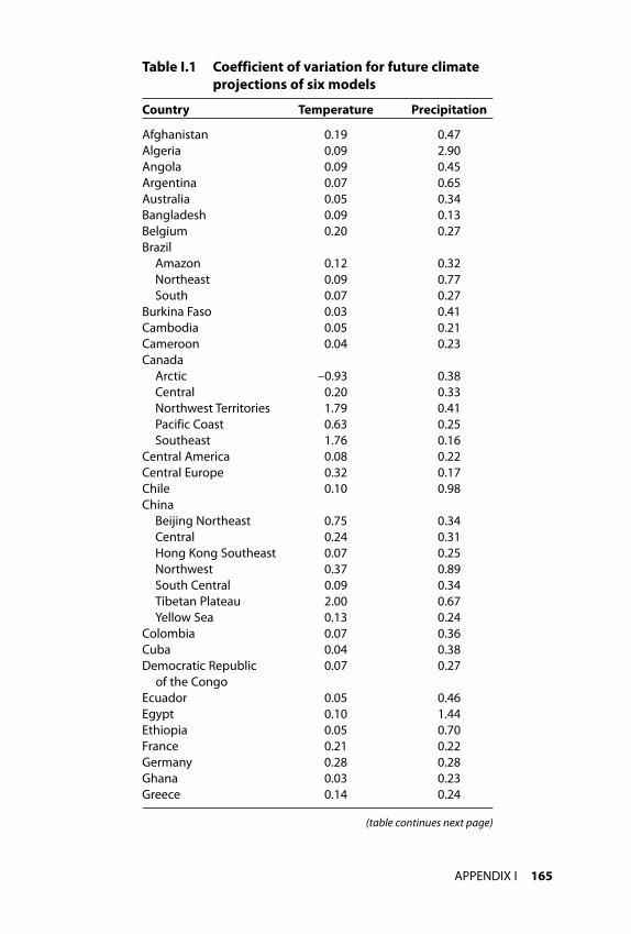
APPENDIX I 165
Table I.1 Coefficient of variation for future climateprojections of six models
Country Temperature Precipitation
Afghanistan 0.19 0.47Algeria 0.09 2.90Angola 0.09 0.45Argentina 0.07 0.65Australia 0.05 0.34Bangladesh 0.09 0.13Belgium 0.20 0.27Brazil
Amazon 0.12 0.32Northeast 0.09 0.77South 0.07 0.27
Burkina Faso 0.03 0.41Cambodia 0.05 0.21Cameroon 0.04 0.23Canada
Arctic –0.93 0.38Central 0.20 0.33Northwest Territories 1.79 0.41Pacific Coast 0.63 0.25Southeast 1.76 0.16
Central America 0.08 0.22Central Europe 0.32 0.17Chile 0.10 0.98China
Beijing Northeast 0.75 0.34Central 0.24 0.31Hong Kong Southeast 0.07 0.25Northwest 0.37 0.89South Central 0.09 0.34Tibetan Plateau 2.00 0.67Yellow Sea 0.13 0.24
Colombia 0.07 0.36Cuba 0.04 0.38Democratic Republic 0.07 0.27
of the CongoEcuador 0.05 0.46Egypt 0.10 1.44Ethiopia 0.05 0.70France 0.21 0.22Germany 0.28 0.28Ghana 0.03 0.23Greece 0.14 0.24
(table continues next page)
02--Appendices--99-168 6/21/07 11:40 AM Page 165
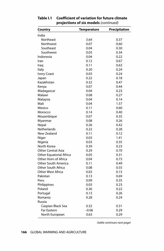
166 GLOBAL WARMING AND AGRICULTURE
IndiaNortheast 3.64 0.37Northwest 0.07 0.60Southeast 0.04 0.30Southwest 0.03 0.34
Indonesia 0.04 0.22Iran 0.12 0.67Iraq 0.11 0.63Italy 0.20 0.24Ivory Coast 0.03 0.24Japan 0.22 0.18Kazakhstan 0.32 0.47Kenya 0.07 0.44Madagascar 0.04 0.23Malawi 0.08 0.27Malaysia 0.04 0.14Mali 0.04 1.57Mexico 0.11 0.60Morocco 0.14 0.40Mozambique 0.07 0.35Myanmar 0.08 0.26Nepal 0.26 0.42Netherlands 0.22 0.28New Zealand 0.11 0.12Niger 0.03 1.41Nigeria 0.03 0.35North Korea 0.39 0.23Other Central Asia 0.29 0.70Other Equatorial Africa 0.05 0.31Other Horn of Africa 0.04 0.73Other South America 0.11 0.49Other South Africa 0.08 0.55Other West Africa 0.03 0.15Pakistan 0.13 0.69Peru 0.09 0.35Philippines 0.03 0.23Poland 0.36 0.22Portugal 0.13 0.26Romania 0.28 0.24Russia
Caspian Black Sea 0.32 0.31Far Eastern –0.06 0.29North European 0.63 0.29
Table I.1 Coefficient of variation for future climateprojections of six models (continued)
Country Temperature Precipitation
(table continues next page)
02--Appendices--99-168 6/21/07 11:40 AM Page 166
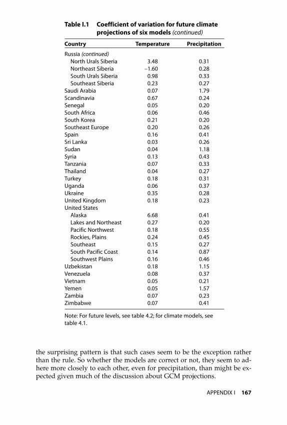
APPENDIX I 167
Russia (continued)North Urals Siberia 3.48 0.31Northeast Siberia –1.60 0.28South Urals Siberia 0.98 0.33Southeast Siberia 0.23 0.27
Saudi Arabia 0.07 1.79Scandinavia 0.67 0.24Senegal 0.05 0.20South Africa 0.06 0.46South Korea 0.21 0.20Southeast Europe 0.20 0.26Spain 0.16 0.41Sri Lanka 0.03 0.26Sudan 0.04 1.18Syria 0.13 0.43Tanzania 0.07 0.33Thailand 0.04 0.27Turkey 0.18 0.31Uganda 0.06 0.37Ukraine 0.35 0.28United Kingdom 0.18 0.23United States
Alaska 6.68 0.41Lakes and Northeast 0.27 0.20Pacific Northwest 0.18 0.55Rockies, Plains 0.24 0.45Southeast 0.15 0.27South Pacific Coast 0.14 0.87Southwest Plains 0.16 0.46
Uzbekistan 0.18 1.15Venezuela 0.08 0.37Vietnam 0.05 0.21Yemen 0.05 1.57Zambia 0.07 0.23Zimbabwe 0.07 0.41
Note: For future levels, see table 4.2; for climate models, seetable 4.1.
Table I.1 Coefficient of variation for future climateprojections of six models (continued)
Country Temperature Precipitation
the surprising pattern is that such cases seem to be the exception ratherthan the rule. So whether the models are correct or not, they seem to ad-here more closely to each other, even for precipitation, than might be ex-pected given much of the discussion about GCM projections.
02--Appendices--99-168 6/21/07 11:40 AM Page 167

02--Appendices--99-168 6/21/07 11:40 AM Page 168
References
ABS (Australian Bureau of Statistics). 2005. Value of Agricultural Commodities Produced, Aus-tralia 2004–05. Canberra. Available at www.abs.gov.au (accessed April 12, 2007).
Adams, R. M., C. Rosenzweig, R. Peart, J. Ritchie, B. McCarl, J. Glyer, B. Curry, J. Jones, K. Boote, and L. Allen. 1990. Global Climate Change and U.S. Agriculture. Nature (May):219–24.
Adams, Richard M., Bruce A. McCarl, Kathleen Segerson, Cynthia Rosenzweig, Kelly J.Bryant, Bruce L. Dixon, Richard Conner, Robert E. Evenson, and Dennis Ojima. 1999.Economic Effects of Climate Change on US Agriculture. In The Impact of Climate Changeon the United States Economy, ed. Robert Mendelsohn and James E. Neumann. Cam-bridge, UK: Cambridge University Press.
Avila, Antonio Flavio Dias, Luiz José Maria Irias, and Magda Aparecida de Lima. 2006.Global Warming Effects on the Brazilian Agriculture: Economic Impact Assessment onLand Values. World Bank, Washington. Photocopy (December).
BEA (Bureau of Economic Analysis). 2006. National Income and Product Accounts. Washington:US Department of Commerce. Available at www.bea.gov (accessed June 29, 2006).
Boer, G., G. Flato, and D. Ramsden. 2000. A Transient Climate Change Simulation withGreenhouse Gas and Aerosol Forcing: Projected Climate to the Twenty-First Century.Climate Dynamics 16, no. 6 (June): 427–50.
Cap, Eugenio, and Jorge Lozanoff. 2006. El Impacto del Cambio Climatico sobre la Agricultura Argentina: Un Estudio Económico. World Bank, Washington. Photocopy (December).
CEA (Council of Economic Advisers). 1994. Economic Report of the President. Washington.Cline, William R. 1992. The Economics of Global Warming. Washington: Peterson Institute for
International Economics.Cline, William R. 1996. The Impact of Global Warming on Agriculture: Comment. American
Economic Review 86, no. 5 (December): 1309–11.Cline, William R. 2004. Climate Change. In Global Crises, Global Solutions, ed. Bjørn Lomborg.
Cambridge, UK: Cambridge University Press.Darwin, Roy, Marinos Tsigas, Jan Lewandrowski, and Anton Raneses. 1995. World Agricul-
ture and Climate Change. Agricultural Economic Report no. 703 (June). Washington: USDepartment of Agriculture, Economic Research Service.
Darwin, R. F. 1999. A FARMer’s View of the Ricardian Approach to Measuring AgriculturalEffects of Climate Change. Climatic Change 41: 371–411.
169
03--References--169-174 6/15/07 10:54 AM Page 169
Darwin, R. F., and D. Kennedy. 2000. Economic Effects of CO2 Fertilization of Crops: Trans-forming Changes in Yield into Changes in Supply. Environmental Modeling and Assess-ment 5, no. 3:157–68.
Deininger, Klaus. 1999. Making Negotiated Land Reform Work: Initial Experiences from Brazil,Colombia, and South Africa. World Bank Policy Research Working Paper no. 2040 (Janu-ary). Washington: World Bank.
Dinar, Ariel, Robert Mendelsohn, Robert Evenson, Jyoti Parikh, Apurva Sanghi, KaviKumar, James McKinsey, and Stephen Lonergan. 1998. Measuring the Impact of ClimateChange on Indian Agriculture. World Bank Technical Paper no. 402 (March). Washington:World Bank.
Emori, S., T. Nozawa, A. Abe-Ouchi, A. Numaguti, M. Kimoto, and T. Nakajima. 1999. Cou-pled Ocean-Atmosphere Model Experiments of Future Climate Change with an ExplicitRepresentation of Sulfate Aerosol Scattering. Journal of the Meteorological Society of Japan77: 1299–307.
EPA (Environmental Protection Agency). 1989. The Potential Effects of Global Climate Changeon the United States, eds. Joel B. Smith and Dennis Tirpak. Washington.
ERS (Economic Research Service). 2006a. China Agricultural and Economic Data. Washington:US Department of Agriculture. Available at www.ers.usda.gov/data/china (accessedJune 29, 2006).
ERS (Economic Research Service). 2006b. Data Sets: International Food Consumption Patterns.Washington: US Department of Agriculture.
FAO (Food and Agriculture Organization). 2005. Compendium of Food and Agriculture Indica-tors 2005. Rome. Available at www.fao.org (accessed June 29, 2006).
FAO (Food and Agriculture Organization). 2006a. World Census of Agriculture: Results byCountry. Rome. Available at www.fao.org (accessed June 29, 2006).
FAO (Food and Agriculture Organization). 2006b. FAO Country Profiles and Mapping Infor-mation System. Rome. Available at www.fao.org.
Federal Register. 2006. US Government. Federal Register 71, no. 158 (August 16).Fischer, Günther, Harrij vanVelthuizen, Mahendra Shah, and Freedy Nachteergaele. 2002.
Global Agro-Ecological Assessment for Agriculture in the 21st Century: Methodology and Re-sults. Laxenburg, Austria: International Institute for Applied Systems Analysis.
Flato, G. M., and G. J. Boer. 2001. Warming Asymmetry in Climate Change Experiments. Geo-physical Research Letters 28: 195–98.
González U., Jorge, Roberto Velasco H., and José Cares G. 2006. Cambio Climático en SistemasAgrícolas de Chile: I: Evaluación Preliminar del Efecto de Variables de Clima Sobre elValor Económico Estimado del Suelo. World Bank, Washington. Photocopy (December).
Gordon, H. B., and S. P. O’Farrell. 1997. Transient Climate Change in the CSIRO CoupledModel with Dynamic Sea Ice. Monthly Weather Review 125: 875–907.
Gordon, C., C. Cooper, C. A. Senior, H. T. Banks, J. M. Gregory, T. C. Johns, J. F. B. Mitchell,and R. A. Wood. 2000. The Simulation of SST, Sea Ice Extents and Ocean Heat Transportsin a Version of the Hadley Centre Coupled Model without Flux Adjustments. ClimateDynamics 16: 147–68.
Hitz, Sam, and Joel Smith. 2004. Estimating Global Impacts from Climate Change. In TheBenefits of Climate Change Policies: Analytical and Framework Issues. Paris: Organisation forEconomic Cooperation and Development.
IBGE (Instituto Brasileiro de Geografia e Estatística). 2006. Censo Agropecuário de 1995–1996.Rio de Janeiro. Available at www.ibge.gov.br (accessed June 29, 2006).
IEA (International Energy Agency). 2006. Energy Technology Perspectives: Scenarios and Strate-gies to 2050. Paris.
IPCC (Intergovernmental Panel on Climate Change). 1996. Climate Change 1995: Impacts,Adaptations and Mitigation of Climate Change: Scientific-Technical Analyses, ed. Robert T.Watson, Marufu C. Zinyuwera, and Richard H. Moss. IPCC Second Assessment Report:Climate Change 1995. Cambridge, UK: Cambridge University Press.
170 GLOBAL WARMING AND AGRICULTURE
03--References--169-174 6/15/07 10:54 AM Page 170
IPCC (Intergovernmental Panel on Climate Change). 1999. Guidelines on the Use of ScenarioData for Climate Impact and Adaptation Assessment, Version 1. IntergovernmentalPanel on Climate Change, Task Group on Scenarios for Climate Impact Assessment (De-cember). Available at http://ipcc-ddc.cru.uea.ac.uk.
IPCC (Intergovernmental Panel on Climate Change). 2001a. Climate Change 2001: The Scien-tific Basis, ed. J. T. Houghton et al. IPCC Third Assessment Report: Climate Change 2001.Cambridge, UK: Cambridge University Press.
IPCC (Intergovernmental Panel on Climate Change). 2001b. Climate Change 2001: Impacts,Adaptation, and Vulnerability, ed. James J. McCarthy et al. IPCC Third Assessment Re-port: Climate Change 2001.Cambridge, UK: Cambridge University Press.
IPCC (Intergovernmental Panel on Climate Change). 2007a. Summary for Policymakers. Cli-mate Change 2007: The Physical Science Basis. Working Group I Contribution to IPCCFourth Assessment Report: Climate Change 2007. Geneva.
IPCC (Intergovernmental Panel on Climate Change). 2007b. Summary for Policymakers. Cli-mate Change 2007: Climate Change Impacts, Adaptation, and Vulnerability. Working GroupII Contribution to IPCC Fourth Assessment Report: Climate Change 2007. Geneva(April 6).
IMF (International Monetary Fund). 2006. International Financial Statistics. Washington.Jativa, Pablo, and S. Niggol Seo. 2006. A Cross-Sectional Examination of Climate Change Im-
pacts on Agriculture in Ecuador. World Bank, Washington. Photocopy (December).Jorgenson, Dale W., Richard J. Goettle, Brian H. Hurd, and Joel B. Smith. 2004. U.S. Market
Consequences of Global Climate Change. Arlington, VA: Pew Center on Global ClimateChange (April).
Knutson, T. R., T. L. Delworth, K.W. Dixon, and R. J. Stouffer. 1999. Model Assessment of Re-gional Surface Temperature Trends (1949–1997). Journal of Geophysical Research 104:30981–96.
Kurukulasuriya, Pradeep, and Shane Rosenthal. 2003. Climate Change and Agriculture. WorldBank Environment Department Paper no. 91 (June). Washington: World Bank.
Kurukulasuriya, Pradeep, Robert Mendelsohn, Rashid Hassan, James Benhin, TemesgenDeressa, Mbaye Diop, Helmy Mohamed Eid, K. Yerfi Fosu, Glwadys Gbetibouo, SumanJain, Ali Mahamadou, Renneth Mano, Jane Kabubo-Mariara, Samia El-Marsafawy,Ernest Molua, Samiha Ouda, Mathieu Ouedraogo, Isidor Sène, David Maddison, S. Nig-gol Seo, and Ariel Dinar. 2006. Will African Agriculture Survive Climate Change? WorldBank Economic Review, no. 21 (October).
Kurukulasuriya, Pradeep, and Robert Mendelsohn. 2006. A Ricardian Analysis of the Impactof Climate Change on African Cropland. CEEPA Discussion Paper no. 8 (July). Pretoria,South Africa: Centre for Environmental Economics and Policy in Africa.
Li, Yi-Fan. 1996. Global Population Distribution Database. Downsview, Ontario: EnvironmentCanada (August 12). Available at http://grid.cr.usgs.gov.
Long, Stephen P., Elizabeth A. Ainsworth, Andrew D. B. Leakey, and Patrick B. Morgan. 2005.Global Food Insecurity: Treatment of Major Food Crops with Elevated Carbon Dioxideor Ozone under Large-scale Fully Open-Air Conditions Suggests Recent Models MayHave Overestimated Future Yields. Philosophical Transactions of the Royal Society B 360:2011–20.
Long, Stephen P., Elizabeth A. Ainsworth, Andrew D. B. Leakey, Josef Nösberger, and Don-ald R. Ort. 2006. Food for Thought: Lower-than-Expected Crop Yield Stimulation withRising CO2 Concentrations. Science 312 (June 30): 1918–21.
Mendelsohn, Robert, William D. Nordhaus, and Daigee Shaw. 1994. The Impact of GlobalWarming on Agriculture: A Ricardian Analysis. American Economic Review 84, no. 4 (Sep-tember): 753–71.
Mendelsohn, Robert, and James E. Neumann, eds. 1999. The Impact of Climate Change on theUnited States Economy. Cambridge, UK: Cambridge University Press.
REFERENCES 171
03--References--169-174 6/15/07 10:54 AM Page 171
Mendelsohn, Robert, and William D. Nordhaus. 1999. The Impact of Global Warming onAgriculture: A Ricardian Analysis: Reply. American Economic Review 89, no. 4 (Septem-ber): 1053–55.
Mendelsohn, Robert, and Michael E. Schlesinger. 1999. Climate Response Functions. Ambio28, no. 4 (June): 362–66.
Mendelsohn, Robert, Wendy Morrison, Michael E. Schlesinger, and Natalia G. Andronova.2000. Country-Specific Market Impacts of Climate Change. Climatic Change 45: 553–69.
Mendelsohn, Robert, Ariel Dinar, and Apurva Sanghi. 2001. The Effect of Development onthe Climate Sensitivity of Agriculture. Environment and Development Economics 6: 85–101.
Mendelsohn, Robert, and Ariel Dinar. 2003. Climate, Water, and Agriculture. Land Economics79, no. 3 (August): 328–41.
Mendelsohn, Robert, and Michelle Reinsborough. 2007. A Ricardian Analysis of US andCanadian Farmland. Yale University, New Haven, CT. Photocopy.
Nakicenovic, N., and R. Swart, eds. 2000. IPCC Special Report on Emissions Scenarios. Cam-bridge, UK: Cambridge University Press.
NAST (National Assessment Synthesis Team). 2001. Climate Change Impacts on the UnitedStates: The Potential Consequences of Climate Variability and Change. Report to the USGlobal Change Research Program. Cambridge, UK: Cambridge University Press.
NOAA (National Oceanic and Atmospheric Administration). 2007. Comparative ClimaticData: Data Tables. Washington: US Department of Commerce. Available at http://ols.nndc.noaa.gov (accessed March 29, 2007).
Nordhaus, William D., and Joseph Boyer. 2000. Warming the World: Economic Models of GlobalWarming. Cambridge, MA: MIT Press.
OECD (Organisation for Economic Cooperation and Development). 2004. The Benefits of Cli-mate Change Policies: Analytical and Framework Issues. Paris.
OECD (Organisation for Economic Cooperation and Development). 2005. OECD in Figures,2005 Edition. Paris. Available at http://ocde.p4.siteinternet.com (accessed June 29, 2006).
Pacheco, Rafael, Luisa Caraballo, and S. Niggol Seo. 2006. Global Warming and Agriculturein Venezuela: An Economic Valuation. World Bank, Washington. Photocopy (December).
Parry, M., C. Rosenzweig, A. Iglesias, G. Fischer, and M. Livermore. 1999. Climate Changeand World Food Security: A New Assessment. Global Environmental Change 9: S51–S67.
Parry, M., C. Rosenzweig, A. Iglesias, M. Livermore, and G. Fischer. 2004. Effects of ClimateChange on Global Food Production under SRES Emissions and Socio-Economic Sce-narios. Global Environmental Change 11, no. 3: 1–3.
Parry, Martin, Cynthia Rosenzweig, and Matthew Livermore. 2005. Climate Change, GlobalFood Supply and Risk of Hunger. Philosophical Transactions of the Royal Society B 360:2125–38 (October 24).
Quiggin, John, and John K. Horowitz. 1999. The Impact of Global Warming on Agriculture: ARicardian Analysis: Comment. American Economic Review 89, no. 4 (September): 1044–45.
Reilly, J., N. Hohmann, and S. Kane. 1994. Climate Change and Agricultural Trade: WhoBenefits, Who Loses? Global Environmental Change 4, no. 1: 24–36.
Reilly, John M., and 22 coauthors. 1996. Agriculture in a Changing Climate: Impacts andAdaptation. In Climate Change 1995: Impacts, Adaptations and Mitigation of Climate Change,ed. Robert T. Watson, Marufu C. Zinyuwera, and Richard H. Moss. Cambridge, UK:Cambridge University Press.
Reilly, John M., and 19 coauthors. 2001. Agriculture: The Potential Consequences of Climate Vari-ability and Change for the United States. US National Assessment of the Potential Conse-quences of Climate Variability and Change, US Global Change Research Program. NewYork: Cambridge University Press.
Reinsborough, Michelle J. 2003. A Ricardian Model of Climate Change in Canada. CanadianJournal of Economics 36, no. 1 (February): 21–40.
172 GLOBAL WARMING AND AGRICULTURE
03--References--169-174 6/15/07 10:54 AM Page 172

Rocha, Jorge Granados, Irma Baquero Haeberlin, Margarita Ramírez Gómez, and FabiolaGómez. 2006. Efectos del Cambio Climático Global en la Agricultura Colombiana.World Bank, Washington. Photocopy (December).
Roeckner, E., K. Arpe, L. Bengtsson, M. Christoph, M. Claussen, L. Dümenil, M. Esch, M. Giorgetta, U. Schlese, and U. Schulzweida. 1996. The Atmospheric General CirculationModel ECHAM-4: Model Description and Simulation of Present-Day Climate. Max-PlanckInstitute for Meteorology Report no. 218. Hamburg, Germany: Max-Planck Institute forMeteorology.
Rosenberg, Norman J., and Pierre R. Crosson. 1991. Processes for Identifying Regional Influencesof and Responses to Increasing Atmospheric CO2 and Climate Change: The MINK Project—AnOverview. DOE/RL/01830T-H5 (August). Washington: US Department of Energy.
Rosenzweig, C., M. L. Parry, G. Fischer, and K. Frohberg. 1993. Climate Change and World FoodSupply. Research Report no. 3. Oxford: University of Oxford, Environmental ChangeUnit. Available at www.ciesin.org (accessed August 9, 2006).
Rosenzweig, Cynthia, and Ana Iglesias, eds. 1994. Implications of Climate Change for Interna-tional Agriculture: Crop Modeling Study. EPA 230-B-94-003. Washington: US Environmen-tal Protection Agency.
Rosenzweig, C., and M. L. Parry. 1994. Potential Impacts of Climate Change on World FoodSupply. Nature 367: 133–38.
Rosenzweig, C., M. Parry, and G. Fischer. 1995. World Food Supply. In As Climate Changes:International Impacts and Implications, ed. K. M. Strzepek and J. B. Smith. Cambridge, UK:Cambridge University Press.
Rosenzweig, Cynthia, and Ana Iglesias. 2006. Potential Impacts of Climate Change on WorldFood Supply: Data Sets from a Major Crop Modeling Study. New York: Goddard Institutefor Space Studies, Columbia University. Available at http://sedac.ciesin.columbia.edu(accessed August 9, 2006).
Sanghi, Apurva, Robert Mendelsohn, and Ariel Dinar. 1998. The Climate Sensitivity of In-dian Agriculture. In Measuring the Impact of Climate Change on Indian Agriculture, byDinar et al. World Bank Technical Paper no. 402 (March). Washington: World Bank.
Statistics Canada. 2007. Agriculture 2001 Census: Data Tables. Ottawa. Available at www.statcan.ca.
Stern Review. 2006. Stern Review Report on the Economics of Climate Change, by Nicholas Stern.Prepublication edition available at www.hm-treasury.gov.uk. Published edition avail-able as The Economics of Climate Change: The Stern Review. Cambridge, UK: CambridgeUniversity Press, 2007.
Tol, Richard S. J. 2002. Estimates of Damage Costs of Climate Change. Environmental and Re-source Economics 21: 47–73.
Tubiello, F. N., C. Rosenzweig, R. A. Goldberg, S. Jagtap, and J. W. Jones. 2002. Effects of Cli-mate Change on US Crop Production: Simulation Results Using Two Different GCMScenarios. Part I: Wheat, Potato, Maize, and Citrus. Climate Research 20 (April): 259–70.
Tubiello, Francesco N., Jeffrey S. Amthor, Kenneth J. Boote, Marcello Donatelli, William East-erling, Gunther Fischer, Roger M. Gifford, Mark Howden, John Reilly, and CynthiaRosenzweig. 2007. Crop Response to Elevated CO2 and World Food Supply. (A Com-ment on “Food for Thought” by Long et al., 2006, Science 312: 1918–21.) European Jour-nal of Agronomy 26: 215–23.
United Nations. 2006. World Population Prospects: The 2004 Revision Population Database. NewYork: United Nations, Department of Economic and Social Affairs.
USDA (US Department of Agriculture). 2004. 2002 Census of Agriculture: Summary and StateData, volume 1. Geographic Area Series, Part 51 (June). Washington.
USDA (US Department of Agriculture). 2005. Cotton and Wool Outlook (December 12).Washington.
REFERENCES 173
03--References--169-174 6/15/07 10:54 AM Page 173
174 GLOBAL WARMING AND AGRICULTURE
USDA (US Department of Agriculture, Foreign Agricultural Service). 2006. World Agricul-tural Production. WAP 09-06 (September). Washington.
Washington, W. M., J. W. Weatherly, G. A. Meehl, A. J. Semtner Jr., T. W. Bettge, A. P. Craig,W. G. Strand Jr., J. Arblaster, V. B. Wayland, R. James, and Y. Zhang. 2000. ParallelClimate Model (PCM): Control and Transient Solutions. Climate Dynamics 16, no. 10-11(October): 755–74.
World Bank. 1978. World Development Report 1978. Washington.World Bank. 1984. World Development Report 1984. Washington.World Bank. 2005. World Development Indicators 2005. Washington.World Bank. 2006. World Development Indicators 2006. Washington.Worldwatch Institute. 1998. United States Leads World Meat Stampede. Washington (July 1).Zhang, X-H., J. M. Oberhuber, A. Bacher, and E. Roeckner. 1998. Interpretation of Interbasin
Exchange in an Isopycnal Ocean. Climate Dynamics 14: 725–40.
03--References--169-174 6/15/07 10:54 AM Page 174
Glossary
benchmark 2 � CO2 warming. Eventual equilibrium warming from adoubling of atmospheric concentration of carbon dioxide above prein-dustrial levels (280 parts per million by volume, or ppm, prior to the In-dustrial Revolution). The present concentration of CO2 is about 380 ppm.Equilibrium climate simulations commonly assume a radiative forcingequivalent to a doubling of preindustrial CO2 concentration.
C3 and C4 crops. Crops are generally divided into two groups—C3 andC4—depending on the number of carbon atoms in the first stable com-pound into which carbon dioxide is incorporated during photosynthesis(process by which plants use sunlight to make carbohydrates from CO2and water, with oxygen as a waste product). Plants belonging to the C3group include rice, wheat, soybeans, barley, oats, potatoes, fine grains,legumes, and most trees. Those in the C4 group include maize, millet,sorghum, and sugarcane. Because of differences in the photosynthesisprocess between the two groups, C3 crops benefit substantially more thanC4 crops from “carbon fertilization” associated with higher atmosphericconcentrations of CO2.
carbon dioxide equivalent. Measure that expresses the amount of othergreenhouse gases in terms of the amount of carbon dioxide that wouldhave the same global warming potential.
carbon fertilization. Enhancement of the growth of plants as a result ofincreased atmospheric carbon dioxide concentration, resulting from thefact that CO2 is an input into the process of photosynthesis.
175
04--Glossary--175-178 6/21/07 11:29 AM Page 175
crop process models. Agronomic models that predict yields and other as-pects of crop production as a function of temperature, precipitation, avail-ability of irrigation, soil type, crop management, and other variables.
equilibrium climate simulation. Mode of running a global climate modelin which greenhouse gas concentrations are suddenly changed (typicallydouble the preindustrial values) and the model allowed to come intoequilibrium with the new forcing (see also benchmark 2 ¥ CO2 warmingand ocean thermal lag).
evapotranspiration. Combined loss of moisture from soil through evapo-ration and from plants through stomatal transpiration.
free air concentration enrichment (FACE). Method whereby carbon di-oxide levels can be elevated in a specified area of forest or other biomass.Unlike controlled environments such as growth chambers and green-houses, this experiment enables scientists to study the response of plantgrowth to increased levels of CO2 under natural conditions.
general circulation models (GCMs). Computer models of the earth’s cli-mate system that simulate the physical processes whereby the atmo-sphere and oceans affect global climate. They have been developed overtwo decades and require extensive computations to run. They can be runto estimate current climates and the sensitivity of climate to different con-ditions such as different levels of greenhouse gases.
greenhouse gas emissions. Release of gases from the burning of fossilfuels for residential, commercial, and industrial purposes and to powertransport vehicles (automobiles, trucks, airplanes, trains, and ships) andfrom other emissions-producing processes and activities. Globally theseemissions are measured in gigatons (1 billion metric tons).
greenhouse effect. Warming of the earth attributable to the opacity ofwater vapor, carbon dioxide, and other greenhouse gases to outboundlong-wave infrared radiation from the earth, relative to their transpar-ency to inbound short-wave solar radiation. The result of this differentialis that about half of the sun’s radiation is permitted to enter through theatmosphere, but about 80 to 90 percent of the returning radiation from the earth is trapped. Natural greenhouse gases keep the earth’s averagesurface temperature about 33°C warmer than it otherwise would be (atabout +15°C rather than –18°C). In its 2007 report, the IntergovernmentalPanel on Climate Change judged that anthropogenic (manmade) emis-sions of greenhouse gases have been the main reason for the observed risein average global surface temperatures by about 0.8°C from 1850–99 to2001–05.
176 GLOBAL WARMING AND AGRICULTURE
04--Glossary--175-178 6/21/07 11:29 AM Page 176

Kyoto Protocol. Agreement made under the United Nations FrameworkConvention on Climate Change. Industrial and transition-economy, butnot developing, countries that ratify this protocol commit to reducingtheir emissions of carbon dioxide and five other greenhouse gases by atleast 5 percent below 1990 levels in the commitment period 2008–2012 orengage in emissions trading if they maintain or increase emissions ofthese gases (see greenhouse gas emissions). The protocol was negotiatedin Kyoto, Japan in December 1997 and came into force on February 16,2005 following ratification by Russia in November 2004. As of October2006, a total of 166 countries and other governmental entities have ratifiedthe agreement (representing over 61.6 percent of emissions). Notable ex-ceptions include the United States and Australia. Although India andChina have ratified the protocol, as developing countries they are not re-quired to reduce carbon emissions despite their large populations and (es-pecially in the case of China) current emissions.
MMSA. Mendelsohn, Morrison, Schlesinger, and Andronova (2000).
MS. Mendelsohn and Schlesinger (1999).
ocean thermal lag. Length of time (some three decades for benchmark 2 ¥CO2 warming) between increase in atmospheric concentration of green-house gases and the resulting eventual equilibrium warming, attributableto ocean thermal dynamics. During this period surface warming is slowedas the deep ocean is warmed to maintain an equilibrium differential fromocean surface temperatures.
permanent crop land. Land under crops that last many seasons and arenot replanted after each harvest. Permanent crops include tea, coffee, rub-ber, flowering shrubs, fruit and nut trees, and vines.
Ricardian models. Family of Ricardian or cross-section (CS) models re-lating agricultural capacity to temperature and precipitation, usually in anonlinear fashion, on the basis of statistical estimates from farm survey orcounty-level data across varying climatic zones. The classical economistDavid Ricardo developed the theory that the value of land depends on the difference between its fertility and that of the least fertile land justbrought into cultivation at the margin. The seminal Ricardian agriculturalimpact model (Mendelsohn, Nordhaus, and Shaw 1994) argued that sta-tistical regressions relating land values to climate differences could cap-ture the impact of climate on agricultural productivity and thus be usedto calculate prospective effects of global warming.
GLOSSARY 177
04--Glossary--175-178 6/21/07 11:29 AM Page 177
SRES scenarios. A suite of emissions scenarios developed by the Inter-governmental Panel on Climate Change (IPCC) in its Special Report onEmissions Scenarios (SRES) for the Third Assessment Report and alsoused in the Fourth Assessment Report. The six families of scenarios areA1FI, A1B, A1T, A2, B1, and B2. The central scenario set used in the pre-sent study is SRES A2, in which carbon dioxide emissions rise from about7.3 GtC (gigatons of carbon) in 1990 to about 29 GtC by 2100.
transient climate simulation. Mode of running a global climate model inwhich a period of time is simulated with continuously varying concen-trations of greenhouse gases so that the climate of the model representsprospective changes already realized by the time of each future date inquestion, rather than the higher long-run equilibrium warming eventu-ally resulting from atmospheric concentrations at each such date. The dif-ference stems from ocean thermal lag.
Sources: The present study; Cline (1992); IPCC Data Distribution Center, www.ipcc-data.org; US Department of Agriculture, www.usda.gov; Environmental Pro-tection Agency, www.epa.gov; United Nations Environment Program, www.unep.org; Pew Center on Global Climate Change, www.pewclimate.org; and UnitedNations Framework Convention on Climate Change, http://unfccc. int. All Websites accessed on June 8, 2007.
178 GLOBAL WARMING AND AGRICULTURE
04--Glossary--175-178 6/21/07 11:29 AM Page 178
Index
179
abatement, 97costs of, 18–19, 29
Adams, Richard, 134Adams et al. (1990) study, 18Adams et al. (1999) study, 45, 134adaptation
costs of, 62in crop models, 29, 62crop yields with, 14, 21in Darwin (1995) study, 17farm-level, supply impact of, 13in MS model, 45
Africaagricultural production in, 50, 50nclimate models for, 84–85, 139tdryland agriculture in, 53, 54t–55t, 56,
84, 139tirrigation in, 53, 54t–55t, 56, 84, 137–38,
139tMMSA study results, 83Ricardian models for, 48, 48n, 50,
51t–52t, 53, 63, 139tvulnerable regions of, 21, 80, 96World Bank study on, 49–56, 84–85
agricultural capacitychanges in, regional aggregates, 76, 77t,
78in Ricardian models, 129–35, 130t–33t
agricultural impact of global warming,1–2
country-level estimates of (See country-specific models; specific country)
dynamic considerations, 87–94by major regions, 79metastudy of, 19summary estimates on, 95–96, 96tsurvey of existing literature on, 7–21synthesis of preferred estimates on,
63–80, 67t–71t, 74f–75fagricultural import barriers, 33agricultural land. See also farm area
classification by growing season length,11–12
database on, 6diversion to ethanol biomass
production, 87, 89, 93agricultural output
business as usual projections for, 87by country, region, and subzone,
115–18, 119t–21tdatabase on, 6land rental value and, 46–47, 47tland zone model of, 13by major regions, 78–80, 79tin MMSA study, 81–82MS model of, 124, 125t–28tnet revenue from climate change and,
48n, 48–49synthesis of preferred estimates on, 66,
67t–71t
05--Index--179-186 6/15/07 10:55 AM Page 179
agricultural output—continuedtrade effects and, 33value of, 115
agricultural potentialpercent change in, 73, 73n, 74, 76fsummary estimates on, 95–96, 96t
agricultural production. See also cropyields
benchmark warming and, 20general circulation models of, 16land zone model of, 13of major crops, 90t, 90–91preferred estimates of, 72–73, 74f–75fRicardian estimates of, 48in Rosenzweig-Iglesias studies, 85threshold levels for, 20–21, 41
agricultural response functions, in MSmodel, 43–46
agroecological zone model, 15–17air temperature, 41, 41n, 95Argentina, 140tAsia
crop yields in, 21rice production in, 91vulnerability of, 80
Australiafarm area and output in, 116subzones of, 112tthreshold level for, 41vulnerability of, 97water availability in, 21wheat production in, 91n
barley, 62baseline emissions scenario, 4basic linked system (BLS), 32nbenchmark 2 × CO2 warming, 7–10
agricultural production and, 20economic effects of, 11in Tol (2002) study, 17
biofuel production, land diversion for, 87,89, 93
Boer, Flato, and Ramsden (2000) study, 57Brazil
farm area and output in, 116Mendelsohn et al. (2001) study on, 48nMMSA study results, 83Ricardian models for, 140tsubzones of, 112tWorld Bank study on, 48n, 58
business as usual projections, 4, 59for agricultural output, 87, 95global effects under, 96–97synthesis of, 72
Canadaclimate models, 14, 16–17, 47, 58–59,
65, 65ncrop models, 16farm area and output in, 117MMSA study results, 82subzones of, 112t
capital outlays, for irrigation, 29–32carbon dioxide
atmospheric concentration of, in MSmodel, 44–45
in photosynthesis, 24, 24ncarbon fertilization effect, 11, 23–26, 48, 82
agricultural capacity and, 76, 77t, 78agricultural productivity and, 73, 75fin crop models, 62definition of, 3estimation of, 24–25failure to materialize, 95global versus regional aggregates, 78global weighted effect of, 135on maize, 20by major regions, 78–80, 79tin MS model, 25–26, 26n, 124, 125t–28t,
129–35, 130t–33tsynthesis of estimates on, 65–66, 66n,
67t–71t, 72, 96, 96tCCC (Climate Crisis Coalition) model, 57C3 crops, 24, 24nC4 crops, 24, 24nCCSR (Center for Climate Change
Research) model, 36t, 57, 101–104CGCM1 model, 16nCGCM2 model, 36t, 104Chile, 140tChina
agricultural production in, 9, 72, 90–91farm area and output in, 116–17geopolitics in, 97MMSA study results, 83subzones of, 112tvulnerability of, 80
climate. See also precipitation;temperature
monthly data on, 142t–61tclimate change. See global warmingclimate models, 35–37, 36t. See also
general circulation models (GCMs)country-specific, 3, 37, 38t–40t, 41–42
(See also specific country)Ricardian estimates dispersed across,
59, 60t, 61in Rosenzweig-Iglesias studies, 85standardized grids for, 6, 101–104
180 GLOBAL WARMING AND AGRICULTURE
05--Index--179-186 6/15/07 10:55 AM Page 180
climate projections, dispersion acrossGCMs, 163–64, 165t–67t, 167
climate sensitivity parameters, 37, 83Cline (1992) study, 8, 13, 32–33Cline (2004) study, 37coefficient of variation, for climate
projections, 164, 165t–67tconsensus climate projection, 3, 59, 61consumer surplus, 33, 33ncosts
abatement, 18–19, 29adaptation, 62irrigation, 29–32transition, 20
countries, regions, and subzones (CRSs).See also specific country or region
definition of, 111farm area and output by, 115–18,
119t–21tmonthly climate data for, 142t–61t
country-specific models, 5. See also specificcountry
climate, 3, 37, 38t–40t, 41–42versus global aggregates, 78mapping grid cells in, 105–108MS functions applied to, 63–80, 123–35Ricardian, 129–35, 130t–33tstandardization of, 6, 101–104technological change and, 91
crop(s). See also specific cropbiofuel, 87–88mix of (See adaptation)prices of, 10, 72, 91, 91nprincipal world producers of, 89–91, 90ttemperature thresholds for, 10water demand by, temperature and, 10
crop models, 3, 5adaptation lacking in, 29agricultural potential change in, 73,
73n, 74, 76fversus agroecological zone models, 16meta-analysis of, 19–20regional aggregates of, 76, 77t, 78versus Ricardian estimates, 78, 134–35in Rosenzweig-Iglesias studies, 8–9,
61–63synthesis of, 63, 64t, 65–66, 67t–71t, 73,
74f–75f, 96, 96tcrop yields, 9–10. See also agricultural
productionwith adaptation, 14, 21by latitude, 19for major crops, 91, 92tprices and, 11
regional tables for, 10, 10ntechnological change and, 87, 89temperature thresholds and, 18–20trade and, 32n, 32–33trends in, 89–91, 90t
cross-section (CS) models. See Ricardianmodels
CSIRO model, 36t, 104
Darwin et al. (1995) study, 6, 11, 13, 17, 20
Darwin (1999) study, 29–30Darwin and Kennedy (2000) study, 24demand
for agricultural products (See fooddemand)
crop water, temperature and, 10developing countries. See also specific
countrycrop yields in, 9effects of trade on, 32–33general circulation models of, 16latitude and, 18, 49, 49nmeat consumption in, 93t, 93–94, 94nMMSA study results, 83Ricardian estimates for, 47–58synthesis of estimates on, 78–80, 79t,
96, 96tthreshold level for, 41vulnerability of, 1–2, 7, 95–97
drought, 19, 29dryland agriculture, in Africa, 53, 54t–55t,
56, 84, 139t“dumb farmer” critique, 29“Dutch disease,” 59n
ECHAM4/OPYC3 model, 16n, 36t, 104Ecuador, 140tEgypt, 53, 56, 84, 137–38Emori et al. (1999) study, 57energy crops, land diversion to, 87, 89, 93Engel’s law, 88Environmental Protection Agency (EPA)
studies, 7–9Environment Canada, 105nequilibrium warming, 98ethanol biomass production, 87, 89Europe, 21, 80nevapotranspiration, 9–10, 26
farm area. See also agricultural landby country, region, and subzone,
115–18, 119t–21tversus geographical area, 115–16
INDEX 181
05--Index--179-186 6/15/07 10:55 AM Page 181
farm area—continuedsynthesis of preferred estimates on, 66,
67t–71tweighting by, 41–42, 42t
fertilizer, changes in. See adaptationFischer et al. (2002) study, 15–17Food and Agriculture Organization (FAO)
agricultural censuses, 116food quantity estimates, 91nSoil Map of the World, 15
food demand, 87income elasticity of, 88, 88f, 89npopulation growth and, 93price inelasticity of, 33, 33n, 72versus supply, 91–93
food products, major groupings of, 15free air concentration enrichment (FACE)
method, 24–25, 63, 66, 135future agricultural resources model
(FARM), 12
general circulation models (GCMs), 2, 4,35–37, 36t, 104
country-level, 3, 37, 38t–40t, 41–42dispersion of climate projections across,
163–64, 165t–67t, 167grid standardization for, 4, 6, 101–104
geographical area, 3–4versus farm land area, 115–16of grid cells, calculating, 109
geopolitics, 97GFDL (Geophysical Fluid Dynamics
Laboratory) model, 9, 12, 36t, 64t, 85,104
GISS (Goddard Institute for SpaceStudies) model, 9, 12, 64t, 85
Global Population Distribution Database,105–106
global warmingagricultural impact of (See agricultural
impact of global warming)analysis of (See also climate models)
relevant period for, 2to date, 41, 41nequilibrium, 98limiting, 97
costs of, 18–19, 29grain consumption, versus meat
consumption, 93–94greatest common divisor (GCD), 102grid cells
geographical area of, calculating, 109mapping to countries, 105–108
grid code number, definition of, 106
GridCtry dataset, 106–108grid land area, calculation by latitude, 6grid resolution, 4, 82ngrid standardization, 6, 101–104
Hadley Centre for Climate Prediction andResearch, 19
climate models, 14, 36t, 62, 62n, 63n,64t, 104
harvesting, timing of. See adaptationHitz and Smith (2004) study, 18hunger, risk of, 10, 21, 86
“ice to ice” cases, 128import barriers, agricultural, 33income elasticity, of food demand, 88, 88f,
89nIndia
agricultural production in, 49, 58, 72carbon fertilization effect in, 49climate models for, 83–84, 138tfarm area and output in, 117geopolitics in, 97Ricardian models for, 17, 48, 48n, 49,
49n, 50t, 65, 83–84, 138tsubzones of, 112tthreshold level for, 41vulnerability of, 80
industrial countries. See also specificcountry
meat consumption in, 93t, 93–94, 94nsynthesis of estimates on, 78–80, 79t, 96,
96tthreshold level for, 41
Intergovernmental Panel on ClimateChange (IPCC), 2
Second Assessment Report, 10–11, 62,80
Third Assessment Report, 37, 62, 84–85Fourth Assessment Report, 20–21, 37Data Distribution Centre, 35–36, 101Special Report on Emissions Scenarios
(SRES), 25, 36–37, 41–42, 62, 85–86Working Group II contribution to
Fourth Assessment Report, 20International Energy Agency, 89international trade, as moderator, 32–33irrigation, 26–32
in Africa, 53, 54t–55t, 56, 84, 137–38,139t
capital outlays for, 29–32changes in (See adaptation)costs of, 29–32general circulation models of, 16
182 GLOBAL WARMING AND AGRICULTURE
05--Index--179-186 6/15/07 10:55 AM Page 182
need for, and climate change, 26–27,28f, 30
in US, 26–27, 28fwater availability for, 9, 16, 26, 29,
84–85irrigation compensation, 84iso-production curves, for MS model, 44f,
44–45
Jorgensen et al. (2004) study, 18
kelvin, 163, 164nKurukulasuriya et al. (2006) study, 48, 53,
63, 84–85Kurukulasuriya and Mendelsohn (2006)
study, 85Kyoto Protocol, 97
land area. See also agricultural land; farmarea
by country, region, and subzone,115–18, 119t–21t
ratio of farm land to, 115–16weighting by, 41–42, 42t
land class coverage, percent changes in,12
land classification, 5–6by growing season length, 11–12by utilization type, 15–16, 16n
land rental equivalent, in Ricardianestimates, 25–26, 129–35, 130t–33t
land rental value, output potential and,46–47, 47t
land surface air temperature, 41, 41n, 95land value models, 5, 57, 57tland zone model, 11, 13–14
in Fischer (2002) study, 15–17versus Rosenzweig model, 13
Latin America. See also specific countryagricultural production in, 58Ricardian models for, 56–58, 57t, 83,
138–39, 140tvulnerability of, 80, 96World Bank study on, 48, 48n, 56–58,
57t, 65, 85latitude
agroecological zone model by, 16crop yields by, 19grid land area calculations by, 6land zone model approach to, 12regional differences due to, 9, 18, 49,
49n, 73, 74f–75f, 95–96Long et al. (2005) study, 24Long et al. (2006) study, 25n
maizecarbon fertilization effect on, 20ethanol produced from, 89production of, 90t, 90–91Rosenzweig model on, 62temperature thresholds for, 10yield impacts, 9–10, 91, 92t
mapping methodology, 115–16meat consumption per capita, 93t, 93–94,
94nMendelsohn, Dinar, and Sanghi (1998)
study, 17Mendelsohn, Dinar, and Sanghi (2001)
study, 48, 48n, 49, 49n, 50t, 65, 83–84
Mendelsohn and Dinar (2003) study, 32nMendelsohn, Morrison, Schlesinger, and
Andronova (2000) study (MMSA), 20,81–83
carbon fertilization effect in, 25–26, 26n,82
grid specification in, 82nversus MS model, 46positive effects found in, 2turning point identified in, 41
Mendelsohn, Nordhaus, and Shaw (1994)model, 4–5, 45, 63n
irrigation in, 29quadratic functional form in, 20
Mendelsohn and Nordhaus (1999) studyirrigation in, 29–31mathematical error in, 30n, 30–31
Mendelsohn and Reinsborough (2007)study, 58–59
Mendelsohn, Robert, 3, 63nMendelsohn and Schlesinger (1999) study
(MS model), 5adaptation in, 45agricultural response functions in,
43–46carbon fertilization effect in, 25, 124,
125t–28t, 129–35, 130t–33tcountry-specific results for, 6, 63–80,
123–35crop models in, 65dispersion across climate models, 59,
60t, 61versus MMSA model, 46reduced form, 43–46, 123–29, 125t–28tfor US, 46–47, 47t, 63, 133–34
MINK study, 8model-source studies, estimates in,
comparison to, 80–86monthly climate data, 142t–61t
INDEX 183
05--Index--179-186 6/15/07 10:55 AM Page 183
multicountry regions, 113multiple cropping, general circulation
models of, 16
Nakiçenoviç and Swart (2000) study, 36–37national climate data, mapping from 1°
cell assignments to, 107–108New Zealand, 73Nordhaus and Boyer (2000) study, 17
ocean thermal lag, 2, 2n, 98Organization for Economic Cooperation
and Development (OECD), 18, 115OSU (Oregon State University) model, 12output. See agricultural output
Parry et al. (1999) study, 18Parry, Rosenzweig, and Livermore (2005)
study, 20, 73n, 85–86PCM (Parallel Climate Model), 57per capita income
food demand and, 88, 88f, 89nmeat consumption and, 93–94
planting, timing of. See adaptationpopulation growth, 87–88
food demand and, 93population movements, 20potatoes, 10precipitation
in crop models, 62dispersion across GCMs, 163–64,
165t–67t, 167estimated change in, 9, 42, 42nevaporative demand and, 10land versus farm area weighting for,
41–42, 42tmodels of, 35–37
country-specific, 37, 38t–40t, 41–42monthly data on, 152t–61tin MS model, 44–45and need for irrigation, 26–27, 28f, 30
price(s)land zone model of, 13of major crops, 10, 72, 91, 91nyield reductions and, 11
price inelasticity, of food demand, 33, 33n,72
producer surplus, 33, 33nproduction. See agricultural production;
crop yieldspurchasing power parity (PPP) income
per capitafood demand and, 88, 88f, 89nmeat consumption and, 93–94
quadratic functional form, 20Quiggin and Horowitz (1999) study, 29
regions, 6. See also specific regiondefinition of, 111farm area and output by, 115–18, 119t–21tmulticountry, 113
Reilly et al. (1994) study, 11Reilly et al. (2001) study, 14–15, 18, 20Reinsborough (2003) study, 58–59, 65, 65nRicardian agricultural impact function, in
MS model, 45Ricardian models, 3–5. See also specific
studyof agricultural capacity, 76, 77t, 78of agricultural potential, 73, 73n, 74, 76fof carbon fertilization effect, 25–26country-specific, 129–35, 130t–33t
versus global aggregates, 78versus crop models, 78, 134–35for developing countries, 47–58dispersed across climate models, 59,
60t, 61irrigation in, 29–32synthesis of, 65–66, 67t–71t, 73, 74f–75f,
96, 96tRicardo, David, 4rice
production of, 90t, 90–91Rosenzweig model on, 62temperature thresholds for, 10yield impacts, 9–10, 91, 92t
Rosenberg and Crosson (1991) study, 8Rosenzweig, Cynthia, 3Rosenzweig and Iglesias (1994) study,
8–9, 85–86crops models in, 63, 64tpreferred regional aggregate results, 76,
77t, 78Rosenzweig and Iglesias (2006) study, 5,
59, 63n, 86crop model results, 61–63
Rosenzweig and Parry (1994) study, 20Rosenzweig et al. (1993) study, 11
crop models in, 8–9versus land zone model, 13
Rosenzweig et al. (1995) study, 18RuBisCO, 24nRussia
crop models, 16farm area and output in, 117, 117nnew agricultural land in, 13Ricardian models of, 59, 59n, 65, 82subzones of, 112t
184 GLOBAL WARMING AND AGRICULTURE
05--Index--179-186 6/15/07 10:55 AM Page 184

seasonal variationin developing countries, 48–50in temperature, 31, 31n
sea surface air temperature, 41, 41nsensitivity to climate models, 59–61, 60tSoil Map of the World (FAO/UNESCO),
15solar radiation, in crop models, 62soybeans
production of, 90t, 90–91Rosenzweig model on, 62yield impacts, 9–10, 91, 92t
Special Report on Emissions Scenarios(SRES), 25, 36–37, 41–42, 62, 85–86
Stern Review (2006), 18–20subzones, 6
definition of, 111farm area and output by, 115–18,
119t–121tof largest countries, 112t
sugarcane, ethanol produced from, 89supply. See also crop yields
changes in, 13versus demand, 91–93dynamic influences on, 89farm-level adaptation and, 13population growth and, 93trade effects and, 33, 33n
technological change, 6country-specific estimates of, 91crop yields and, 87, 89
temperatureagricultural production and, 20–21air, 41, 41n, 95in crop models, 62crop yields and, 18–20dispersion across GCMs, 163–64,
165t–67t, 167food groupings by, 15land versus farm area weighting for,
41–42, 42tmodels of, 35–37
country-specific, 37, 38t–40t,41–42
monthly data on, 142t–51tin MS model, 44–45and need for irrigation, 26–27, 28f, 30seasonal variation in, 31, 31n
temperature scales, 163, 163n–64ntemperature thresholds, 9–10, 82terms-of-trade losses, 32–33thermal climate categories, 15Tol (2002) study, 2, 17–18
trade as moderator, 32–33transition costs, 20Tubiello et al. (2007) study, 25n
UKMO (United Kingdom MeteorologicalOffice) model, 9, 12, 64t, 85
United Kingdom, Stern Report from,18–20
United Nations, population projections,87–88
United Nations Environment Program(UNEP), Global ResourceInformation Database (GRID), 105n
United Statesagricultural output of, 115n, 117, 117n,
124nagricultural production in, 58, 72,
90–91Alaska, 12–13, 15, 128Iowa, 8climate model, 15Corn Belt, 12crop models for, 5, 9, 65EPA study on, 7–8farm area in, 117, 117n, 124nfood quantity estimates, 91nGDP originating in agriculture for, 47,
47nirrigation in, 26–27, 28fKansas, 8land zone model, 12Missouri, 8MMSA model for, 83MS model for, 46–47, 47t, 63, 133–34Nebraska, 8Nevada, 27, 27nReilly (2001) study on, 14–15subzones of, 112tthreshold level for, 41Utah, 27vulnerability of, 97Wyoming, 27
US Department of Agriculture (USDA)Economic Research Service (USDA),
11–14Global Change Research Program,
14–15, 18–201995 study, 11–14
US Department of Energy, 8US Global Change Research Program,
14US National Assessment of the Potential
Consequences of Climate Variabilityand Change, 14
INDEX 185
05--Index--179-186 6/15/07 10:55 AM Page 185
Washington et al. (2000) study, 57water availability
in Australia, 21for irrigation, 9, 16, 26, 29, 84–85
water demand, effect of temperature on, 10water stress, adverse effects of, 19weather events, short-term, 20welfare loss, 32–33wheat
production of, 90t, 90–91
Rosenzweig model on, 62temperature thresholds for, 10yield impacts, 9, 14n, 91, 92t
World Bank studies, 84–85Africa, 49–56, 63Latin America, 48, 48n, 56–58, 57t,
65, 85world food trade model, 8
yields. See crop yields
186 GLOBAL WARMING AND AGRICULTURE
05--Index--179-186 6/15/07 10:55 AM Page 186