global trajectory optimisation: can we prune the solution ... study report/act-rpt-mad-ari-06... ·...
TRANSCRIPT

Global Trajectory Optimisation: Can We Prune the Solution
Space when Considering Deep Space Maneuvers?
Final Report Authors: F. Bernelli-Zazzera, M. Lavagna, R. Armellin, P. Di Lizia, F. Topputo Affiliation: Aerospace Engineering Department, Politecnico di Milano Authors: M. Berz Affiliation: Department of Physics and Astronomy, Michigan State University ESA Researcher(s): Tamás Vinkó Date: December 2007 Contacts: Franco Bernelli-Zazzera Tel: +39 02 2399 8328 Fax: +39 02 2399 8334 e-mail: [email protected]
Leopold Summerer Tel: +31(0)715655174 Fax: +31(0)715658018 e-mail: [email protected]
Available on the ACT website http://www.esa.int/act
Ariadna ID: 06/4101 Study Duration: 6 months
Contract Number: 2007/06/NL/HI

ii

Contents
Abstract 1
1 Introduction 3
2 Notes on Di!erential Algebra 92.1 The Minimal Di!erential Algebra . . . . . . . . . . . . . . . . 102.2 The Di!erential Algebra nDv . . . . . . . . . . . . . . . . . . . 142.3 Solution of Parametric Implicit Equations . . . . . . . . . . . 16
3 GASP-DA: Analysis and Implementation 193.1 DA-evaluation of the objective function . . . . . . . . . . . . . 19
3.1.1 Parametric implicit equations . . . . . . . . . . . . . . 213.2 The discontinuity problem . . . . . . . . . . . . . . . . . . . . 26
3.2.1 Box-reshaping and box-splitting . . . . . . . . . . . . . 303.2.2 Planar planetary model . . . . . . . . . . . . . . . . . 34
3.3 The dependency problem . . . . . . . . . . . . . . . . . . . . . 373.4 Semi-analytical approximation . . . . . . . . . . . . . . . . . . 40
3.4.1 Kepler’s equation . . . . . . . . . . . . . . . . . . . . . 403.4.2 Lagrange’s equation . . . . . . . . . . . . . . . . . . . 423.4.3 Bending angle equation . . . . . . . . . . . . . . . . . . 43
3.5 Quadratic polynomial bounder . . . . . . . . . . . . . . . . . . 463.6 Test cases . . . . . . . . . . . . . . . . . . . . . . . . . . . . . 47
3.6.1 The optimization process . . . . . . . . . . . . . . . . . 493.6.2 EM . . . . . . . . . . . . . . . . . . . . . . . . . . . . . 513.6.3 EV . . . . . . . . . . . . . . . . . . . . . . . . . . . . . 523.6.4 EJ . . . . . . . . . . . . . . . . . . . . . . . . . . . . . 533.6.5 EVM . . . . . . . . . . . . . . . . . . . . . . . . . . . . 543.6.6 EMJ . . . . . . . . . . . . . . . . . . . . . . . . . . . . 563.6.7 EVME . . . . . . . . . . . . . . . . . . . . . . . . . . . 573.6.8 EVVEJS . . . . . . . . . . . . . . . . . . . . . . . . . . 58
3.7 Final remarks . . . . . . . . . . . . . . . . . . . . . . . . . . . 61

iv CONTENTS
4 Introduction of DSM in GASP-DA 634.1 Preliminary Considerations . . . . . . . . . . . . . . . . . . . . 644.2 Forward Propagation Strategy . . . . . . . . . . . . . . . . . . 66
4.2.1 Planet-to-Planet Case . . . . . . . . . . . . . . . . . . 664.2.2 MGA Case . . . . . . . . . . . . . . . . . . . . . . . . 67
4.3 Absolute Variables Strategy . . . . . . . . . . . . . . . . . . . 694.3.1 Planet-to-Planet Case . . . . . . . . . . . . . . . . . . 694.3.2 MGA Case . . . . . . . . . . . . . . . . . . . . . . . . 70
4.4 Implementation of GASP-DSM-DA . . . . . . . . . . . . . . . 724.5 Test Cases . . . . . . . . . . . . . . . . . . . . . . . . . . . . . 74
4.5.1 EdM . . . . . . . . . . . . . . . . . . . . . . . . . . . . 754.5.2 EMdJ . . . . . . . . . . . . . . . . . . . . . . . . . . . 764.5.3 EMdMJ . . . . . . . . . . . . . . . . . . . . . . . . . . 774.5.4 EVdVEJ . . . . . . . . . . . . . . . . . . . . . . . . . . 784.5.5 EVEdEJ . . . . . . . . . . . . . . . . . . . . . . . . . . 794.5.6 EdVdM . . . . . . . . . . . . . . . . . . . . . . . . . . 804.5.7 EVdMdE . . . . . . . . . . . . . . . . . . . . . . . . . 814.5.8 EVdVEJS . . . . . . . . . . . . . . . . . . . . . . . . . 824.5.9 EVdVEJdS . . . . . . . . . . . . . . . . . . . . . . . . 83
4.6 Final Remarks . . . . . . . . . . . . . . . . . . . . . . . . . . . 83
5 Alternative Approach for MGA-DSM Transfers 855.1 Solution Set Selection . . . . . . . . . . . . . . . . . . . . . . . 865.2 DSM modeling . . . . . . . . . . . . . . . . . . . . . . . . . . 875.3 First Guess Generation . . . . . . . . . . . . . . . . . . . . . . 895.4 Problem Formulation . . . . . . . . . . . . . . . . . . . . . . . 895.5 Test Cases . . . . . . . . . . . . . . . . . . . . . . . . . . . . . 90
5.5.1 EVM . . . . . . . . . . . . . . . . . . . . . . . . . . . . 905.5.2 EMJ . . . . . . . . . . . . . . . . . . . . . . . . . . . . 925.5.3 EVME . . . . . . . . . . . . . . . . . . . . . . . . . . . 935.5.4 EMMJ . . . . . . . . . . . . . . . . . . . . . . . . . . . 945.5.5 EVEEJ . . . . . . . . . . . . . . . . . . . . . . . . . . 955.5.6 EVVEJS . . . . . . . . . . . . . . . . . . . . . . . . . . 96
5.6 Final Remarks . . . . . . . . . . . . . . . . . . . . . . . . . . . 97
6 Validated Optimization of MGA Transfers 996.1 Di!erential Algebra and Interval Arithmetic . . . . . . . . . . 996.2 Remainder-enhanced Di!erential Algebraic
Operations . . . . . . . . . . . . . . . . . . . . . . . . . . . . 1016.2.1 Addition and Multiplication . . . . . . . . . . . . . . . 1036.2.2 Intrinsic Functions . . . . . . . . . . . . . . . . . . . . 105

CONTENTS v
6.2.3 Derivations and Antiderivations . . . . . . . . . . . . . 1076.3 Examples . . . . . . . . . . . . . . . . . . . . . . . . . . . . . 108
6.3.1 A Simple Function . . . . . . . . . . . . . . . . . . . . 1086.3.2 Bound Enclosures of Functions . . . . . . . . . . . . . 111
6.4 Notes on COSY-GO . . . . . . . . . . . . . . . . . . . . . . . 1136.5 Validated Solution of Implicit Equations . . . . . . . . . . . . 1146.6 Test Cases . . . . . . . . . . . . . . . . . . . . . . . . . . . . . 116
6.6.1 EM . . . . . . . . . . . . . . . . . . . . . . . . . . . . . 1166.6.2 EVM . . . . . . . . . . . . . . . . . . . . . . . . . . . . 117
6.7 Final Remarks . . . . . . . . . . . . . . . . . . . . . . . . . . . 118
7 Conclusions and Final Remarks 121
Bibliography 127

vi CONTENTS

List of Figures
1.1 Messenger . . . . . . . . . . . . . . . . . . . . . . . . . . . . . 5
3.1 An Earth–Mars transfer . . . . . . . . . . . . . . . . . . . . . 203.2 Search space sampling for the Earth–Mars transfer . . . . . . 213.3 Orbital elements . . . . . . . . . . . . . . . . . . . . . . . . . 223.4 Powered gravity assist . . . . . . . . . . . . . . . . . . . . . . 233.5 Taylor expansions: position error . . . . . . . . . . . . . . . . 253.6 Taylor expansions: velocity error . . . . . . . . . . . . . . . . 253.7 !V for the Earth–Mars transfer . . . . . . . . . . . . . . . . . 263.8 Taylor expansion accuracy on !V . . . . . . . . . . . . . . . . 263.9 !V for the EM transfer . . . . . . . . . . . . . . . . . . . . . 283.10 !V for the EM transfer after pruning . . . . . . . . . . . . . . 283.11 Enclosure of the pruned !V on the overall search space . . . . 293.12 Enclosure of the pruned !V on the pruned search space . . . 293.13 Discontinuities on the !V . . . . . . . . . . . . . . . . . . . . 293.14 Short–way to long–way discontinuity: geometrical view . . . . 303.15 Short–way to long–way discontinuity: objective function . . . 303.16 The approximate slope of the discontinuities . . . . . . . . . . 313.17 Sample box before reshaping . . . . . . . . . . . . . . . . . . . 313.18 Sample box after reshaping . . . . . . . . . . . . . . . . . . . . 313.19 Enclosure using reshaped boxes . . . . . . . . . . . . . . . . . 323.20 Box splitting procedure: splitting lines . . . . . . . . . . . . . 333.21 Box splitting procedure: box division . . . . . . . . . . . . . . 333.22 Short–way to long–way discontinuity in 2D model . . . . . . . 343.23 Long–way to short–way discontinuity in 2D model . . . . . . . 343.24 Short–way to long–way discontinuity: 3D vs. 2D . . . . . . . . 353.25 !V in the 3D model . . . . . . . . . . . . . . . . . . . . . . . 353.26 !V in the 2D model . . . . . . . . . . . . . . . . . . . . . . . 353.27 Pruned search space in the 3D model . . . . . . . . . . . . . . 363.28 Pruned search space in the 2D model . . . . . . . . . . . . . . 363.29 GASP–DA on the 2D model . . . . . . . . . . . . . . . . . . . 37

viii LIST OF FIGURES
3.30 GASP–DA on the 3D model . . . . . . . . . . . . . . . . . . . 373.31 EMJ transfer . . . . . . . . . . . . . . . . . . . . . . . . . . . 383.32 Design space for the EM arc . . . . . . . . . . . . . . . . . . . 383.33 Design space for the MJ arc . . . . . . . . . . . . . . . . . . . 383.34 Dependencies in the EMJ transfer . . . . . . . . . . . . . . . . 403.35 !V in the TE ! TM plane: overall search space . . . . . . . . 413.36 !V in the TE ! TM plane: pruned search space . . . . . . . . 413.37 Semi-analytical solution: position error . . . . . . . . . . . . . 423.38 Semi-analytical solution: velocity error . . . . . . . . . . . . . 423.39 !V for the EM transfer . . . . . . . . . . . . . . . . . . . . . 443.40 !V for the EM transfer: semi–analytical approach . . . . . . 443.41 Semi-analytical approach: bending angle . . . . . . . . . . . . 453.42 Validated bounds based on LDB . . . . . . . . . . . . . . . . . 463.43 Non–validated quadratic bounder . . . . . . . . . . . . . . . . 463.44 Performances of the non–validated quadratic bounder . . . . . 483.45 Performances of the non–validated quadratic bounder: detail . 483.46 Heuristics for box selection . . . . . . . . . . . . . . . . . . . . 503.47 Best identified EM transfer . . . . . . . . . . . . . . . . . . . . 513.48 Best identified EV transfer . . . . . . . . . . . . . . . . . . . . 533.49 Best identified EJ transfer . . . . . . . . . . . . . . . . . . . . 543.50 Best identified EVM transfer . . . . . . . . . . . . . . . . . . . 553.51 Best identified EMJ transfer . . . . . . . . . . . . . . . . . . . 563.52 Best identified EVME transfer . . . . . . . . . . . . . . . . . . 583.53 VV arc: long–way to short–way solution . . . . . . . . . . . . 593.54 VV arc: multi-revolution solution . . . . . . . . . . . . . . . . 593.55 Best identified EVVEJS transfer . . . . . . . . . . . . . . . . . 603.56 Best identified EVVEJS transfer: detail . . . . . . . . . . . . . 60
4.1 A planet-to-platet transfer . . . . . . . . . . . . . . . . . . . . 654.2 Forward propagation: the planet-to-planet case . . . . . . . . 674.3 Forward propagation: the MGA case . . . . . . . . . . . . . . 684.4 Absolute variables: the planet-to-planet case . . . . . . . . . . 704.5 Absolute variables: the MGA case . . . . . . . . . . . . . . . . 714.6 Optimal EdM transfer . . . . . . . . . . . . . . . . . . . . . . 754.7 Optimal EMdJ transfer . . . . . . . . . . . . . . . . . . . . . . 764.8 Optimal EMdMJ transfer . . . . . . . . . . . . . . . . . . . . 774.9 Optimal EVdVEJ transfer . . . . . . . . . . . . . . . . . . . . 784.10 Optimal EVEdEJ transfer . . . . . . . . . . . . . . . . . . . . 794.11 Optimal EdVdM transfer . . . . . . . . . . . . . . . . . . . . . 804.12 Optimal EVdMdE transfer . . . . . . . . . . . . . . . . . . . . 814.13 Optimal EVdVEJS transfer . . . . . . . . . . . . . . . . . . . 82
LIST OF FIGURES ix
4.14 Optimal transfers to jupiter . . . . . . . . . . . . . . . . . . . 84
5.1 Alternative approach algorithmic flow . . . . . . . . . . . . . . 855.2 Cassini-like transfer solution set (1) . . . . . . . . . . . . . . . 865.3 Cassini-like transfer solution set (2) . . . . . . . . . . . . . . . 865.4 Dominance relations . . . . . . . . . . . . . . . . . . . . . . . 875.5 DSM model: heliocentric and planetary view . . . . . . . . . . 885.6 EVM1 optimal trajectory . . . . . . . . . . . . . . . . . . . . . 915.7 EVM2 optimal trajectory . . . . . . . . . . . . . . . . . . . . . 915.8 EMJ optimal trajectory . . . . . . . . . . . . . . . . . . . . . 935.9 EMJ transfer, set on non-dominated solutions . . . . . . . . . 935.10 EVME optimal trajectory . . . . . . . . . . . . . . . . . . . . 945.11 EMMJ optimal trjectory . . . . . . . . . . . . . . . . . . . . . 955.12 EVEEJ optimal trajectory . . . . . . . . . . . . . . . . . . . . 955.13 EVVEJS1 optimal trajectory . . . . . . . . . . . . . . . . . . . 975.14 EVVEJS2 optimal trajectory . . . . . . . . . . . . . . . . . . . 97
6.1 Function f(x) = exp(!1/x2) if x "= 0 ; 0 else . . . . . . . . . 1006.2 1D function and its bound enclosures . . . . . . . . . . . . . . 1126.3 Bound enclosures of a 2D function: interval method . . . . . . 1136.4 Bound enclosures of a 2D function: RDA method . . . . . . . 1196.5 Objective function values and optimal solution found . . . . . 1206.6 !v cuto" history . . . . . . . . . . . . . . . . . . . . . . . . . 120
7.1 ConstraintCOSYGO2 . . . . . . . . . . . . . . . . . . . . . . . 1257.2 ConstraintCOSYGO1 . . . . . . . . . . . . . . . . . . . . . . . 125

x LIST OF FIGURES
List of Tables
3.1 Bounds and box-size for the EM transfer . . . . . . . . . . . . 273.2 Minimum pericenter radii. . . . . . . . . . . . . . . . . . . . . 483.3 Search space and best identified solution for the EM transfer. . 513.4 Search space and best identified solution for the EV transfer. . 523.5 Search space and best identified solution for the EJ transfer. . 533.6 Search space and best identified solution for the EVM transfer. 543.7 Search space and best identified solution for the EMJ transfer. 563.8 Search space and best identified solution for the EVME transfer. 573.9 Search space and best identified solution for the EVVEJS
transfer. . . . . . . . . . . . . . . . . . . . . . . . . . . . . . . 60
4.1 Bounds for the auxiliary variables . . . . . . . . . . . . . . . . 734.2 EdM, time bounds and amplitudes . . . . . . . . . . . . . . . 754.3 EMdJ, time bounds and amplitudes . . . . . . . . . . . . . . . 764.4 EMdMJ, time bounds and amplitudes . . . . . . . . . . . . . . 774.5 EVdVEJ, time bounds and amplitudes . . . . . . . . . . . . . 784.6 EVEdEJ, time bounds and amplitudes . . . . . . . . . . . . . 794.7 EdVdM, time bounds and amplitudes . . . . . . . . . . . . . . 804.8 EVdMdE, time bounds and amplitudes . . . . . . . . . . . . . 814.9 EVdVEJS, time bounds and amplitudes . . . . . . . . . . . . 82
5.1 Time bounds and optimal solution for EVM1 . . . . . . . . . . 905.2 Time bounds and optimal solution for EVM2 . . . . . . . . . . 915.3 Optimal transfers !v [km/s]. . . . . . . . . . . . . . . . . . . 925.4 Time bounds and optimal solution for EMJ. . . . . . . . . . . 925.5 Time bounds and optimal solution for EVME . . . . . . . . . 935.6 Time bounds and optimal solution for EMMJ . . . . . . . . . 945.7 Time bounds and optimal solution for EVEEJ . . . . . . . . . 965.8 Time bounds and optimal solution for EVEEJS1 . . . . . . . . 965.9 Time bounds and optimal solution for EVVEJS2 . . . . . . . . 97

xii LIST OF TABLES
6.1 Elementary properties of interval arithmetic . . . . . . . . . . 1016.2 The total number of FP operations to bound a function . . . . 1116.3 Time bounds and enclosure of the EM optimal solution . . . . 1176.4 Time bounds and enclosure of the EVM optimal solution . . . 118
7.1 Comparison of the three developed methods . . . . . . . . . . 123

Abstract
It has been recently shown that the solution space of multiple gravity assistoptimization problems can be pruned considerably in polynomial time. Thebasic idea behind this technique is to reduce the problem into a cascade oftwo dimensional subproblems and to prune the design space by evaluatingthe objective function and the constraints on a grid which samples the de-sign space. When deep space maneuvers are introduced the complexity ofthe problem increases considerably due to the necessarily added dimensions,and to the larger number of local minima introduced. This study consid-ers di!erential algebraic techniques as an e!ective tool to attach this moredemanding problem. As far as di!erential algebra is used, the objective func-tion and the constraints of the problem are represented by Taylor series ofdesired order, over boxes in which the design domain is split. Thanks to thepolynomial representation of the function and the constraints, a coarse gridcan be used and an e"cient design space pruning can be performed. Fur-thermore, once the domain has been pruned, a suitable manipulation of thepolynomials can ease the subsequent local optimization process, so avoidingthe use of any stochastic optimiser. These two aspects, connected with ane"cient management of the list of boxes in which the design space can bedecomposed, make di!erential algebraic techniques a powerful tool for thedesign of multiple gravity assist transfers including deep space maneuvers, sosupporting the achievement of a further step to fully automate the trajectorydesign problem. Additional e!ort is devoted to develop alternative strategiesfor the ultimate goal of optimizing multiple gravity assist transfers involv-ing deep space maneuvers, and to investigate the performances of validatedglobal optimization techniques on typical space trajectory design problems.
Key words: Global optimisation, solution space pruning, di!erential alge-braic techniques, multiple gravity assist, deep space maneuver.

2 Abstract

Chapter 1
Introduction
Interplanetary space trajectories are usually designed in the frame of thepatched-conics technique. In this context, di!erent conic arcs, solutions of anumber of Lamberts problems, are linked together to define the whole transfertrajectory suitable for the mission considered. The patched-conics methodis based on a two-body representation of the dynamics and on instantaneousvelocity changes provided by chemical high thrust engines.
The patched-conics method allows the designer to define multiple grav-ity assist (MGA) transfers: complex trajectories made up by a sequence ofplanet-to-planet transfers in which the spacecraft exploits each planet en-counter to achieve a velocity change. This method is well established inastrodynamics, and several past missions have used MGA trajectories toreach both inner and outer planets. It is remarkable the case of the Voyagerspacecraft that flew-by Jupiter, Saturn, Uranus, and Neptune exploiting a“lucky” configuration of these planets to leave the Solar System. The firstMGA trajectories were designed by hand with ad hoc methods developedfor a specific mission. In these cases, it was important to find a solution tothe problem, rather than to find the best solution. This was due to the highdegree of complexity given by the relative motion of the planets. The moreplanets were encountered, the more di"cult was to find a feasible solution.
In the last two decades, mission designers have exploited the benefits ofapproaching complex MGA problems from a global optimization standpoint.Nowadays, the aim of the trajectory design is not only to find a solution,but also to find the best solution in terms of propellant consumption, whilestill achieving the mission goals. In the formalism of global optimization,this means that the problem consists in looking for the optimal solutionin those regions of the search space that satisfy the problem constraints.Unfortunately, the MGA problems are characterized by an objective functionwith a large number of clustered minima, which are prevalently associated

4 Introduction
to the complex relative motion of the planets involved in the transfer, andto the nonlinearities governing the simple Kepler’s problem. This causeslocal optimization gradient–based methods to converge to one of these localminima. Hence, despite their e!ciency, Newton–based methods should beavoided when looking for the global minimum of a MGA problem, at leastin the first stage of the search process. This means that global optimizationalgorithms should be used to find the best solution to a MGA problem.However, such algorithms might be computationally ine!cient if used as“black box” tools due to the high dimensions of the search space, and to thelandscape of the objective function cited above. Thus, the key point wouldbe the use of a global optimization algorithm, able to exploit the structureof the search space and the nature of the MGA problem itself.
It has been shown that the solution space of a MGA optimization prob-lem can be pruned considerably in polynomial time. This observation wassuccessfully coded in the gravity assist space pruning (GASP) algorithm [23].The basic idea behind this algorithm is reducing the problem into a cascadeof two–dimensional sub–problems, and pruning the design space by eval-uating the objective function and the constraints on a sampling grid. Inthis way, the search space is pre–processed, and further global optimizationalgorithms are employed in the reduced domain. This procedure showedbetter performances if compared with the standard implementation of somestochastic global optimization solvers over the entire search space. Conse-quently, the combination of a systematic technique (space pruning) and astochastic global optimiser (di"erential evolution, multiple or simple parti-cle swarm optimization, genetic algorithm) produces remarkable numericalburden reduction.
Further improvements are obtained by formalizing the problem in termsof epochs, so avoiding redundant ephemeris evaluations. For instance, bysampling a two–dimensional search space into k cells in each dimension only2k ephemeris evaluations are required and only k2 Lambert’s problems needto be solved. Furthermore, the search space can be remarkably reduced (i.e.pruned) by approaching the problem as a cascade of two-dimensional sub-problems: inequality constraints are evaluated over the grid characterisingeach sub-problem, and unfeasible regions are propagated forward and back-ward and pruned from the whole search space. It is worth noting that thistechnique cannot be applied to any global optimization problem, but it hasbeen developed exploiting the structure of MGA problems.
Unfortunately, the class of MGA transfers so formulated do not cover allthe possible trajectories for a chemical propelled spacecraft. An importantfeature to take into account is the possibility to perform deep space maneu-vers (DSM) that are usually carried out to improve the performances of a

Introduction 5
Figure 1.1: The Messenger MGADSM trajectory.
particular trajectory. When DSM are included into a MGA transfer, theresulting trajectory is usually referred to as MGADSM.
The importance of MGADSM is illustrated with an example. Figure 1.1shows the nominal transfer trajectory for the NASA’s Messenger spacecraftthat is intended to insert into an orbit around Mercury in 2011 after flying-bythe Earth (one time), Venus (two times), and Mercury itself (three times).Finding a feasible solution to such a problem is one of the most challengingtasks in astrodynamics. Probably, the solution would not have been possibleif several DSM had not been included. As clearly shown in Figure 1.1, thenominal solution involves five DSM to be performed during the whole trans-fer. The aim of each DSM is the correction of the trajectory to get an optimalapproach with the body to be encountered. The idea is that the gain givenby this optimal flyby is worth the propellant spent in the maneuver. It isclear that the introduction of DSM, for chemical propelled spacecraft, givessome degrees of freedom that can be exploited not only to perform bettergravity assists, but also to have encounters that would not be possible oth-erwise. A problem so formulated would cover all the possible trajectories fora chemical propelled spacecraft. Furthermore, a MGADSM trajectory canbe applied as first guess solution for the design of low-thrust gravity assisttransfers, where the thrust arcs can spread the impulsive velocity changesgiven by the DSM. In any case, if the solution space of a MGADSM problemcould be pruned, the reward would be enormous. It would be possible todefine a trajectory having an arbitrary number of ballistic arcs, deep spacemaneuvers, and low-thrust arcs (if exponential sinusoids [22] are included in

6 Introduction
the formulation of the problem).Nevertheless, pruning the solution space when deep space maneuvers are
included is not a trivial task. First of all, the dimension of the search spaceincreases because the generic trajectory leg is described by four or even fivevariables if out-of-plane maneuvers are included. Consequently, di!cultiesare introduced in the maneuver modelling as well as in the definition ofsuitable bounds for the introduced variables.
Another feature associated to the MGADSM problem is the proliferationof local minima, that makes di!cult the detection of big prunable regions. Ithas been shown that the search space can be pruned in regions far from thelocal minima where the inequality constraints are not satisfied. In a MGAproblem these are large regions that can be pruned in each two–dimensionalproblem. These regions can become even larger when forward and backwardconstraining are applied, reducing sensibly the final search space. WhenMGADSM is considered, the problem has a much greater number of localminima than a simple MGA problem and the prunable regions are expectedto shrink.
For all the reasons discussed above, it is necessary to rethink the wholepruning process implemented in GASP, and to reformulate it when deepspace maneuvers are included. To handle this problem, the use of di"erentialalgebraic (DA) techniques is proposed in this study.
As better described in chapter 2, di"erential algebra serves the purposeof automatic di"erentiation, i.e. the accurate computation of the derivativesof functions in a computer environment. This goal is actually achieved byreplacing the classical implementation of the real algebra with the properimplementation of a new algebra based on Taylor polynomials. Given ageneric function f of v variables, whose evaluation involves only algebraicoperations (including transcendental functions, inversion, derivation and in-tegration), the Taylor expansion of f up to any desired order n can be easilyobtained from a computer algorithm that implements its evaluation. Therelated derivatives are computed with the accuracy of the floating point rep-resentation of the corresponding real numbers in the computer environment.
The main idea behind the introduction of DA techniques into the pruningprocess is then substituting the pointwise evaluation, typical of GASP, withthe computation of the Taylor expansions of the objective and constraintfunctions with respect to the design variables, around suitably selected ref-erence points of the search space. The Taylor expansions are used to ap-proximate the functions over proper domains. In particular, simple boxesare used, and polynomial bounders are exploited to estimate the ranges ofthe computed functions within each box.
Consequently, using DA techniques, the pointwise approach proposed in

Introduction 7
GASP can be substituted by a sampling process relying on box samples.Thanks to the Taylor approximation, the computation of the tolerance re-lated to the Lipschitzian constant of the GASP method is avoided by usingsuitable bounders of the functions and the corresponding Taylor polynomi-als on the considered domain boxes. Furthermore, as previously mentioned,the order of the Taylor expansion can be exploited to tune the accuracy ofthe approximation and the size of the grid boxes. This might result in thepossibility of enlarging the grid for the domain discretization, and reducingconsiderably the computational burden.
Further interesting information can be drawn from DA computation. Sup-pose that, after the pruning process, the box bounds that possibly enclose theglobal optimum are identified. An optimization process within the identifieddomain is necessary to identify the solution [21]. Savings in computationaltime might be achieved by exploiting the Taylor representation of the ob-jective function over this box. In particular, if the Taylor representation issu!ciently accurate, the further optimization process can be faster processed:the evaluation of the objective function can be substituted by a fast com-putation of polynomials, so exploiting the advantages of metamodel basedglobal optimization algorithms [24].
Based on the previous observations, the first part of the report is devotedto carefully describe the introduction of DA techniques into the classicalGASP algorithm, so dealing with MGA transfers without DSM. In particu-lar, a brief survey on the theory of di"erential algebra is presented in chapter2. Chapter 3 concentrates on the di!culties arising from the introduction ofdi"erential algebra into GASP. The e"ort spent to overcome the discontinu-ity problem and to expand the objective and constraint functions in Taylorseries is deeply examined. The result of this process is the definition of theDA–based GASP algorithm, which will be referred to as GASP–DA in thefollowings. The performances of GASP–DA are then assessed by presentingthe main results of an extensive test phase, relying on suitable MGA transfertest cases.
The major goal of the work is addressed in chapter 4, which is dedicatedto the development of an e"ective pruning algorithm for MGA transfers in-volving DSM. The selection of the most appropriate modeling formulation isthe core of this chapter, as it turned out to strongly a"ect the performancesof the pruning process. The resulting algorithm, referred to as GASP–DSM–DA, is then submitted to a significant test phase, whose results conclude thechapter.
However, the work has not been confined to the achievement of the origi-nally planned scopes. First of all, an alternative strategy to solve the ultimategoal of optimizing MGA transfers including DSM has been developed. The

8 Introduction
strategy is detailed in chapter 5: after a MGA space pruning process, suit-able heuristics are implemented to decide for the introduction of DSM andto define first guess solutions for subsequent optimization processes, aimedat characterizing the resulting MGA-DSM transfers. A comparison analysisof the alternative strategy with GASP–DSM–DA is reported.
Moreover, in the e!ort of paving the way and promoting the use of vali-dated global optimization tools in space–related applications, the validatedglobal optimization of two-impulse transfers is addressed in chapter 6. Taylormodels [26] allow the designer to obtain validated enclosures of the objectivefunction over a box on the search space, and the tool COSY–GO [15] can beused to get bounds of the global optimum.
Final remarks and suggestions for future developments conclude the re-port.

Chapter 2
Notes on Di!erential Algebra
The theory of di!erential algebra presented in this chapter has been devel-oped by Martin Berz in the late 80s, and the short summary given in thefollowing takes advantage of his book Modern Map Methods in Particle BeamPhysics [14].
Di!erential algebraic (DA) techniques find their origin in the attemptto solve analytical problem by an algebraic approach. The DA techniquesintroduced by M. Berz addressed the solution of di!erential equations andpartial di!erential equations, more specifically the e"cient determinationof Taylor expansions of the flow of di!erential equations in terms of initialconditions.
Historically, treatment of functions in numerics has been based on thetreatment of numbers, and the classical numerical algorithms are based on themere evaluation of functions at specific points. DA techniques are based onthe observation that it is possible to extract more information on a functionrather than its mere values. In particular, the Taylor coe"cients of a functioncan be obtained up to a specified order n, along with the function evaluation,with a fixed amount of e!ort. The Taylor coe"cients of order n for sums andproduct of functions, as well as scalar products with reals, can be computedfrom those of summands and factors; therefore, the set of equivalence classesof functions can be endowed with well-defined operations, leading to theso-called truncated power series algebra (TPSA) [3, 4].
Similarly to the algorithms for floating point arithmetic, the algorithm forfunctions followed, including methods to perform composition of functions,to invert them, to solve nonlinear systems explicitly, and to treat commonelementary functions [7, 13]. In addition to these algebraic operations, alsothe analytic operations of di!erentiation and integration have been developedon these function spaces, defining a di!erential algebraic structure.
As DA represents the core of the algorithms developed in the frame of this

10 Notes on Di!erential Algebra
contract, some useful notes to get familiar with these techniques are given inthe following. In particular the minimal di!erential algebra is explained indetails, and some hints on its extension to m variables and to n-th order arethen given. The chapter ends with the description of the solution of implicitparametric equations, necessary to formulate a generic MGA-DSM transferproblem.
2.1 The Minimal Di!erential Algebra
The simplest nontrivial di!erential algebra is here described. Consider allordered pairs (q0, q1), with q0 and q1 real numbers. The addition, scalarmultiplication, and vector multiplication are defined as follows:
(q0, q1) + (r0, r1) = (q0 + r0, q1 + r1)
t · (q0, q1) = (t · q0, t · q1)
(q0, q1) · (r0, r1) = (q0 · r0, q0 · r1 + q1 · r0).
(2.1)
The ordered pairs with the arithmetic are called 1D1. The first two operationsare the familiar vector space structure of R2, whereas the multiplication issimilar to that in the complex numbers; except here (0, 1) · (0, 1) does notequal (!1, 0), but rather (0, 0). The multiplication of vectors is seen to have(1, 0) as the unity element. The multiplication is commutative, associative,and distributive with respect to addition. Together, the three operationsdefined in (2.1) form an algebra. Furthermore, they do form an extension ofreal numbers, as (r, 0)+(s, 0) = (r + s, 0) and (r, 0) · (s, 0) = (r · s, 0), so thatthe reals can be included.
However 1D1 is not a field, as (q0, q1) has a multiplicative inverse in 1D1
if and only if q0 "= 0. If q0 "= 0 then
(q0, q1)!1 =
!
1
q0,!
q1
q20
"
. (2.2)
If q0 is positive, then (q0, q1) # 1D1 has a root
#
(q0, q1) =
!
$q0,
q1
2$
q0
"
, (2.3)
as simple arithmetic shows.
One important property of this algebra is that it has an order compatiblewith its algebraic operations. Given two elements (q0, q1) and (r0, r1) in 1D1,

2.1 The Minimal Di!erential Algebra 11
it is defined
(q0, q1) < (r0, r1) if q0 < r0 or (q0 = r0 and q1 < r1)
(q0, q1) > (r0, r1) if (r0, r1) < (q0, q1)
(q0, q1) = (r0, r1) if q0 = r0 and q1 = r1.
(2.4)
As for any two elements (q0, q1) and (r0, r1) only one of the three relationholds, 1D1 is said totally ordered. The order is compatible with the additionand multiplication; for all (q0, q1), (r0, r1), (s0, s1) ! 1D1, it follows (q0, q1) <(r0, r1) " (q0, q1) + (s0, s1) < (r0, r1) + (s0, s1); and (s0, s1) > (0, 0) = 0 "(q0, q1) · (s0, s1) < (r0, r1) · (s0, s1).
The number d = (0, 1) has the interesting property of being positive butsmaller than any positive real number; indeed
(0, 0) < (0, 1) < (r, 0) = r. (2.5)
For this reason d is called an infinitesimal or a di!erential. In fact, d is sosmall that its square vanishes. Since for any (q0, q1) ! 1D1
(q0, q1) = (q0, 0) + (0, q1) = q0 + d · q1, (2.6)
the first component is called the real part and the second component thedi!erential part.
The algebra in 1D1 becomes a di!erential algebra by introducing a map! from 1D1 to itself, and proving that the map is a derivation. Define ! :
1D1 # 1D1 by
!(q0, q1) = (0, q1). (2.7)
Note that
!{(q0, q1) + (r0, r1)} = !(q0 + r0, q1 + r1) = (0, q1 + r1)
= (0, q1) + (0, r1) = !(q0, q1) + !(r0, r1)(2.8)
and
!{(q0, q1) · (r0, r1)} = !(q0 · r0, q0 · r1 + r0 · q1) = (0, q0 · r1 + r0 · q1)
= (0, q1) · (r0, r1) + (0, r1) · (q0, q1)
= !{(q0, q1)} · (r0, r1) + (q0, q1) · !{(r0, r1)}.(2.9)
This holds for all (q0, q1), (r0, r1) ! 1D1. Therefore ! is a derivation and(1D1, !) is a di!erential algebra.

12 Notes on Di!erential Algebra
The most important aspect of 1D1 is that it allows the automatic com-putation of derivatives. Assuming to have two functions f and g and to puttheir values and their derivatives at the origin in the form (f(0), f !(0)) and(g(0), g!(0)) as two vectors in 1D1, if the derivative of the product f · g isof interest, it has just to be looked at the second component of the product(f(0), f !(0)) · (g(0), g!(0)); whereas the first component gives the value of theproduct of the functions. Therefore, if two vectors contain the values andthe derivatives of two functions, their product contains the values and thederivatives of the product function. Defining the operation [ ] from the spaceof di!erential functions to 1D1 via
[f ] = (f(0), f !(0)), (2.10)
it holds
[f + g] = [f ] + [g]
[f · g] = [f ] · [g](2.11)
and
[1/g] = [1]/[g] = 1/[g] (2.12)
by using 2.2. This observation can be used to compute derivatives of manykinds of functions algebraically by merely applying arithmetic rules on 1D1,beginning from the value and the derivative of the identity function. Considerthe example
f(x) =1
x + 1x
(2.13)
and its derivative
f !(x) =(1/x2) ! 1
(x + (1/x))2. (2.14)
The function value and its derivative at the point x = 3 are
f(3) =3
10, f !(3) = !
2
25. (2.15)
If the function 2.13 is evaluated at the identity function [x] = (x, 1) at thepoint 3, i.e. (3, 1) = 3 + d, it results
f((3, 1)) =1
(3, 1) + 1/(3, 1)=
1
(3, 1) + (1/3,!1/9)
=1
(10/3, 8/9)=
!
3
10,!
8
9/100
9
"
=
!
3
10,!
2
25
"
.
(2.16)

2.1 The Minimal Di!erential Algebra 13
As it can be seen after the evaluation of the function, the real part of theresult is the value of the function at x = 3, whereas the di!erential part isthe value of the derivative of the function at x = 3. This is simply justifiedby applying the relations 2.11 and 2.12
[f(x)] =
!
1
x + 1/x
"
=1
[x + 1/x]
=1
[x] + [1/x]=
1
[x] + 1/[x]
= f([x]).
(2.17)
Since, for a real x, [x] = (x, 1) = x+d, and [f(x)] = (f(x), f !(x)), apparently
(f(3), f !(3)) = f((3 + d)). (2.18)
The method can be generalized to allow the treatment of common intrinsicfunctions, like sin, exp, by setting
gi([f ]) = [gi(f)] or
gi((q0, q1)) = (gi(q0), q1g!i(q0)).
(2.19)
By virtue of equations (2.1) and (2.19) any function f representable byfinitely many additions, subtractions, multiplications, divisions, and intrinsicfunctions in 1D1 satisfies the important relationship
[f(x)] = f([x]). (2.20)
Note that f(r+d) = f(r)+d ·f !(r) resembles f(x+"x) ! f(x)+"x ·f !(x),in which the approximation becomes increasingly more refined for smaller"x. Here, as the "x is infinitely small, the error turns out to be zero.
The di!erential algebra 1D1 allows to compute the first derivative of everyfunction f along with the function evaluation. This has an important con-sequence when the numerical integration of an ordinary di!erential equationis performed by means of an arbitrary integration scheme. Any integrationscheme is based on algebraic operations, involving the evaluations of the ODEright hand side at several integration points; therefore the 1D1 algebra canbe exploited to compute the first order expansion of the flow of the ODE. Asan example consider the first order ordinary di!erential equation
#
x = f(x)x(0) = x0
(2.21)

14 Notes on Di!erential Algebra
and the simple first order forward Euler’s scheme
xk = xk!1 + "t · f(xk!1). (2.22)
If the initial value x0 is substituted by [x0] = (x0, 1) = x0+!x0 ! 1D1 and theiteration scheme is evaluated using 1D1 algebra, the output of the numericalintegration at the k-th step is (xk, "xk/"x0).
By extending the algebra 1D1 to order n and v variables, the expansionsof the flow of a dynamical systems can be computed up to order n with fixedamount of e!ort.
2.2 The Di!erential Algebra nDv
The algebra described in this section was introduced to compute the deriva-tives up to an order n of functions in v variables. Similarly as before, it isbased on taking the space Cn(Rv), the collections of n times continuouslydi!erentiable functions on Rv. On this space an equivalence relation is in-troduced. For f and g ! Cn(Rv), f =n g if and only if f(0) = g(0) and allthe partial derivatives of f and g agree at 0 up to order n. The relation =n
satisfies
f =n f for all f ! Cn(Rv),
f =n g " g =n f for all f, g ! Cn(Rv), and
f =n g and g =n h " f =n h for all f, g, h, ! Cn(Rv).
(2.23)
Thus, =n is an equivalence relation. All the elements that are related to fcan be grouped together in one set, the equivalence class [f ] of the function f .The resulting equivalence classes are often referred to as DA vectors or DAnumbers. Intuitively, each of these classes is then specified by a particularcollection of partial derivatives in all v variables up to order n. This class iscalled nDv.
If the values and the derivatives of two functions f and g are known,the corresponding values and derivatives of f + g and f · g can be inferred.Therefore, the arithmetics on the classes in nDv can be introduced via
[f ] + [g] = [f + g] (2.24)
t · [g] = [t · f ] (2.25)
[f ] · [g] = [f · g]. (2.26)

2.2 The Di!erential Algebra nDv 15
Under this operations, nDv becomes an algebra. For each k ! 1, . . . , v, definethe map !k from nDv to nDv for f via
!k[f ] =
!
pk ·!f
!xk
"
, (2.27)
where
pk(x1, . . . , xk) = xk (2.28)
projects out the k-th component of the identity function. It’s easy to showthat for all k = 1, . . . , v and for all [f ], [g] ! nDv
!k([f ] + [g]) = !k[f ] + !k[g] (2.29)
!k([f ] · [g]) = [f ] · (!k[g]) + (!k[f ]) · [g]. (2.30)
Therefore, !k is a derivation for all k, and hence (nDv, !1, . . . , !k) is a di!er-ential algebra.
The dimension of nDv is now assessed. Define the special numbers dk asfollow:
dk = [xk]. (2.31)
Observe that f lies in the same class as its Taylor polynomial Tf of order naround the origin; they have the same function values and derivatives up toorder n. Therefore,
[f ] = [Tf ]. (2.32)
Denoting the Taylor coe"cients of the Taylor polynomial Tf of f as cj1,...,jv ,it follows
Tf(x1, . . . , xv) =#
j1+···+jv!n
cj1,...,jv · xj11 · · ·xjv
v (2.33)
with
cji, . . . , cjv =
1
j1! · · · jv!·
!j1+···+jvf
!xj11 · · ·!xjv
v
(2.34)
and thus
[f ] = [Tf ] =
$
#
j1+···+jv!n
cj1,...,jv · xj11 · · ·xjv
v
%
=#
j1+···+jv!n
cj1,...,jv · dj11 · · ·djv
v ,
(2.35)

16 Notes on Di!erential Algebra
where, in the last step, the properties [a + b] = [a] + [b] and [a · b] = [a] · [b]have been used. Therefore, the set {1, dk : k = 1, 2, . . . , v} generates nDv,as any element of nDv can be obtained from 1 and the dk’s via addition andmultiplication. Therefore, as an algebra, nDv has (v +1) generators, and theterms dj1
1 · · · djvv form a basis for the vector space nDv. It is shown in [14]
that the number of basic elements is (n + v)!/(n! v!), which is the dimensionon nDv.
Similar to the structure 1D1, nDv can be ordered, and the dk, beingsmaller than any real number, are infinitely small or infinitesimal. Further-more, by applying the fixed point theorem for contracting operators on M !nDv that map M into M , the square root, the quotient, and map inversionin nDv can be obtained by iteration in a finite number of steps. Once thefunction composition and the elementary functions, i.e. exp, sin, and log,are introduced in the DA nDv, the derivatives of any function f belonging toCn(Rv) can be computed up to order n in fixed amount of e!ort by applying
[f(x1, . . . , xv)] = f([x1, . . . , xv]) = f(x1 + d1, . . . , xv + dv). (2.36)
The DA sketched in this section was implemented by M. Berz and K. Makinoin the software COSY INFINITY. The software and all the related documen-tations are available free of charge for non-commercial use online athttp : //bt.pa.msu.edu/index cosy.htm.
2.3 Solution of Parametric Implicit Equations
As it will be explained in the next chapter, the formulation of a MGA transferoptimization problem (either with or without DSM) requires the solution ofparametric implicit equations. This is indeed necessary whenever we wantto solve the Kepler’s equation, the Lagrange’s equation, and the bendingangle equation for the ephemerides evaluation, the Lambert’s problem andthe powered gravity assist problem solution, respectively.
The algorithm developed for the solution of a scalar parametric implicitequation using DA is described; the generalization to the m dimensional caseis straightforward.
We are searching for the solution of
f(x, p) = 0 (2.37)
for p " [pl, pu] with f " Cn+1. This means that x = x(p) satisfying
f(x(p), p) = 0 (2.38)

2.3 Solution of Parametric Implicit Equations 17
is sought. The first step is to consider a point value of the parameter p0 and tocompute the point value of the solution x0 by means of a classical numericalmethod, e.g by Newton’s method. The variable x and the parameter p arethen initialized as n-th order DA variables, i.e.
[x] = x0 + !x
[p] = p0 + !p,(2.39)
and the implicit equation (2.37) is expanded up to the n-th order, deliveringthe map
!f = Mf(!x, !p). (2.40)
Note that the map has no constant part as x0 is the solution of the implicitequation for the nominal value of the parameter p0. The map (2.40) is thenaugmented by introducing the identity map !p = Ip(!p), ending up with
!
!f!p
"
=
!
Mf
Ip
" !
!x!p
"
. (2.41)
The n-th order map (2.41) is inverted using COSY INFINITY built-intools, obtaining
!
!x!p
"
=
!
Mf
Ip
"!1 !
!f!p
"
. (2.42)
As the goal is to compute the n-th order Taylor expansion of the solutionmanifold x = x(p), the map (2.42) is evaluated for !f = 0. From the firstrow we have
!x = M!f=0(!p), (2.43)
which is the n-th order Taylor expansion of the solution manifold, i.e.
!x = !x(!p). (2.44)
For every value of p ! [pl, pu] the approximate solution of f(x, p) = 0 can beeasily computed by evaluating the Taylor polynomial (2.44).

18 Notes on Di!erential Algebra

Chapter 3
GASP-DA: Analysis andImplementation
This chapter is devoted to the accurate description of the introduction ofthe di!erential algebraic techniques into GASP algorithm. The basic idea istaking advantage of the possibility of expanding the constraint and objectivefunctions with respect to the optimization variables. Unfortunately, this isnot an easy task and several problems must be faced. This chapter takescharge of illustrating such problems and their proposed and implementedsolutions.
In particular, section 3.1 describes the procedure to obtain the Taylorexpansion of the constraint and objective functions by expanding the solu-tion of the involved implicit equations. Section 3.2 highlights the presenceof discontinuities on objective functions typically optimized in MGA trans-fers. Rationales for the presence of such discontinuities are supplied, and anextensive analysis is carried out to introduce the proposed solution to theproblem. The mathematical formulation of a typical MGA transfer prob-lem is not unique and a careful selection of the design variables has to beperformed. This is the aim of section 3.3, where the reason of the selectionof the so-called absolute times formulation is pointed out. Some ideas tofurther improve the performances of the optimization process are presentedin sections 3.4 and 3.5. Finally, section 3.6 assesses its performances on testproblems of various complexity.
3.1 DA-evaluation of the objective function
For the sake of a clear description of the topics addressed in this section,and without loss of generality, consider the classical problem of transferring

20 GASP-DA: Analysis and Implementation
Figure 3.1: An Earth–Mars transfer.
a spacecraft from Earth to Mars by means of two impulsive maneuvers (seeFigure 3.1). The typical objective function for this problem is the overallamount of !V that must be supplied to the spacecraft to carry out thetransfer. Two design variables su"ces to this aim. In particular, a possibleand classical choice is selecting the departure epoch from Earth, TE , andthe time of flight from Earth to Mars, tEM . Given TE and tEM , the arrivalepoch at Mars, TM , can be easily computed, and the position and velocityof Earth and Mars at the beginning and the end of the transfer are obtainedthrough ephemerides. Then, given the initial and final positions, and thetime of flight, the corresponding Lambert’s problem is solved to compute theheliocentric initial velocity, v1, the spacecraft must be supplied with at Earthin order to reach Mars in the given time of flight, as well as the resultingheliocentric velocity at Mars, v2. The initial relative velocity of the spacecraftwith respect to Earth, !V 1, and the final relative velocity with respect toMars, !V 2, are readably assessed. A typical optimization problem for thissimple planet-to-planet transfer involves the minimization of the overall !V ,which is computed as the sum of the magnitude of the relative velocities atthe beginning and the end of the transfer:
!V = !!V 1! + !!V 2! = !V1 + !V2, (3.1)
subject to usual constraints on the maximum allowed magnitudes of therelative velocities at the beginning and the end of the transfer:
!V1 " !V1,max
!V2 " !V2,max
(3.2)
As already pointed out in chapter 2, behind the introduction of di#er-ential algebraic techniques is the substitution of the pointwise evaluation of

3.1 DA-evaluation of the objective function 21
Figure 3.2: Search space sampling for the Earth–Mars transfer.
the objective function with a DA–based evaluation. Consequently, insteadof dealing with classical point values of the objective function, the DA-basedGASP algorithm handles its Taylor expansions around suitably selected ref-erence points of the search space. Referring to Figure 3.2, the classical point-wise sampling of the search space implemented in GASP is here replaced bya subdivision of the whole search space in boxes. Then, di!erential algebraictechniques allows to compute the Taylor expansion of the constraint and ob-jective functions within each box around a reference point, e.g. the center ofthe box. The Taylor expansions are bounded to estimate the range of theconstraint and objective functions within the box. The range is then used inthe pruning process. Before detailing the pruning algorithm for this simpleplanet-to-planet transfer, it is worth observing that Taylor expanding theconstraint and objective functions, even for this relatively simple problem,does not lie in a mere DA-based evaluation. The solution of implicit equa-tions is involved in the computation, which poses some additional problems.
3.1.1 Parametric implicit equations
Three implicit equations appear in the evaluation process of constraint andobjective functions for typical MGA transfers. Two of them can be identi-fied by analyzing again the previously introduced Earth–Mars transfer. Theevaluation of the ephemerides of the involved planets is first required. Ananalytical ephemeris model is used within this work, which is based on thirdorder polynomial fits of the orbital elements of the planets (see Figure 3.3).The fitting procedure is performed on a set of accurate values, delivered byJPL ephemeris evaluations. In particular, the analytical model is then ableto supply the eccentricity of the planet orbit, e, and the mean anomaly ofthe planet, M , as a function of the input epoch. At this point, the Kepler’s

22 GASP-DA: Analysis and Implementation
Figure 3.3: Orbital elements.
equation
f(E) = E ! e sin E ! M = 0 (3.3)
must be solved. This is a first implicit equation, which allows to computethe eccentric anomaly, E, from e and M . Therefore, the resulting E is usedto assess the planet position and velocity by mere algebraic relations.
Given the positions of Earth and Mars, and the time of flight betweenthe two planets, the Lambert’s problem must be solved to gain the ini-tial and final heliocentric velocities of the spacecraft. Several algorithmsare available in literature, which tackle this issue from di!erent perspec-tives, and o!er solutions based on di!erent numerical techniques. An un-published algorithm developed by Izzo is used within this work, which isfreely available to download in MATLAB and C++ format from the website:http://www.esa.int/gsp/ACT/inf/op/globopt.htm. The algorithm involvesthe solution of the so-called Lagrange’s equation for the time of flight, thatconcisely reads
f(x) = A(x) ! t = 0 (3.4)
where x is related to the semi–major axis of the resulting transfer orbit, A isa function depending on x and some geometrical properties of the transfer,and t is the transfer time between the involved planets. The solution of thissecond implicit equation allows to compute the initial and final heliocentricvelocities of the spacecraft, by means of algebraic relations and the evaluationof transcendental functions.

3.1 DA-evaluation of the objective function 23
rp
!
planetocentric hyperbole
impulsev
in
!
vout
!
voutp
vinp
!vp
Figure 3.4: Powered gravity assist.
The third implicit equation can be identified only within interplanetarytransfers involving one gravity assist at least. As highlighted in [21], inthe patched-conics approximation, two subsequent heliocentric ellipses mustbe matched using the gravity assist maneuver. This means the pericenterradius of the hyperbolic planetocentric trajectory linking the two heliocentricarcs must be evaluated. To this aim, the classical powered gravity assistmaneuver is implemented: the spacecraft is allowed to provide an impulse atthe pericenter of the incoming hyperbola, tangential to the trajectory (seeFigure 3.4). The planetocentric trajectory is therefore made by two arcs ofhyperbola patched together. Within this model, the angle !, usually referredto as bending angle, between the incoming and the outgoing velocities, vin
!
and vout! respectively, is related to the pericenter radius via
f(rp) = arcsina"
a" + rp+ arcsin
a+
a+ + rp! ! = 0 (3.5)
where a" = 1/(vin! · vin
!) and a+ = 1/(vout! · vout
! ). Given the two heliocentricarcs to be connected by the powered gravity assist maneuver, the angle !can be easily computed through geometrical relations. The solution of thethird implicit equation (3.5) delivers the pericenter radius of the planetocen-tric trajectory. The planetocentric velocities vin
p and voutp at the pericenter,
corresponding to the incoming and outgoing hyperbolic arcs respectively, areevaluated using rp, vin
!, and vout! . Then, the required impulsive maneuver at
the pericenter, !vp, is the mere di"erence between voutp and vin
p .If a pointwise evaluation of the objective and constraint functions is of
interest, as in GASP algorithm, a classical numerical method for the solution

24 GASP-DA: Analysis and Implementation
of implicit equations can be used, e.g. the Newton’s method. Unfortunately,the previous implicit equations become parametric implicit equations whenthe Taylor expansion of the objective and constraint functions is of inter-est. Without loss of generality, consider the Kepler’s equation. In particular,referring to the previous Earth–Mars transfer, the objective function evalua-tion process involves the computation of the planetary ephemerides of Earthand Mars. If the Taylor expansion of the objective function with respectto the design variables is needed, the expansion of the position and velocityof the planets has manifestly to be achieved. The Taylor expansion of theplanetary orbital elements with respect to the epoch can be easily obtainedby initializing the epoch as a DA variable
[T ] = T0 + !T = (T0, 1), (3.6)
where T0 is a point reference epoch, and performing a DA–based evaluationof the analytical ephemeris model. Thus, the Taylor expansions T of theeccentricity and the mean anomaly with respect to the epoch are readilyavailable:
e(!T ) = Te(!T )
M(!T ) = TM (!T ).(3.7)
The next step is solving the Kepler’s equation to compute the correspondingeccentric anomaly E. However, interest is not in a mere point value of E inthis case, but rather in the Taylor expansion of the solution E with respectto the parameter T . Indeed, the explicit dependence of e and M on T mustbe kept and Kepler’s equation reads
f(E, !T ) = E ! e(!T ) sinE ! M(!T ) = 0. (3.8)
The solution of this parametric implicit equation is attained in terms of theTaylor expansion E(!T ) = TE(!T ) using techniques illustrated in chapter2. Once E(!T ) is available, the Taylor expansions of the planet positionand velocity are readily obtained by carrying out the remaining algebraicmanipulations in the DA framework. Clearly, the accuracy of the expansiondepends on the order of the DA computation as well as on the size of theinterval on the epoch, i.e. on !T . Figure 3.5 and Figure 3.6 study this accu-racy referring to Mars ephemerides. In particular, the reference epoch 1456MJD is selected, which corresponds to the arrival date of Mars Express. TheTaylor expansion of Mars position and velocity around the reference epochis computed using di!erential algebra. Considering an interval of 40 daysaround the reference epoch, for each !T , the position and velocity of Mars

3.1 DA-evaluation of the objective function 25
1440 1445 1450 1455 1460 1465 1470 147510
!16
10!14
10!12
10!10
10!8
10!6
10!4
10!2
TM
[MJD]
po
sitio
n e
rro
r [A
U]
3rd
order
5th
order
10th
order
Figure 3.5: Accuracy of the Taylorexpansion of the planet position.
1440 1445 1450 1455 1460 1465 1470 147510
!14
10!12
10!10
10!8
10!6
10!4
10!2
TM
[MJD]
ve
locity e
rro
r [k
m/s
]
3rd
order
5th
order
10th
order
Figure 3.6: Accuracy of the Taylorexpansion of the planet velocity.
are evaluated using both the Taylor expansions and the pointwise evalua-tions. Figure 3.5 and Figure 3.6 report the error of the Taylor expansionswith respect to the pointwise evaluation, in terms of the maximum normof the di!erence vectors between the corresponding positions and velocities,respectively. The figures clearly show that, although the accuracy of theTaylor expansion decreases while moving away from the reference date, itcan be e!ectively kept to a suitable level increasing the expansion order. Itis worth mentioning that the fast wiggling of the curve in the vicinity of thereference epoch is due to the tolerance set for the Newton method, which isused in the classical pointwise ephemeris evaluation.
Similar statements hold for the solution of the Lagrange’s equation (3.4)and for the bending angle equation (3.5). In particular, the ephemeris eval-uation and the solution of the Lambert’s problem, allow to compute theoverall "V for the simple Earth-Mars transfer. For the sake of a more com-plete analysis of the accuracy of the DA computations, Figure 3.8 illustratesan instance of the error of the Taylor expansion of the "V with respect toits point evaluation. The reference epoch 1249 MJD for the departure fromEarth and the reference transfer time of 207 days are selected, which corre-spond to the data of Mars Express. An interval of 40 days is considered foreach variable, representing a box centered on the previous reference pointin the search space. Similarly to the previous analysis, the overall "V isevaluated by a pointwise computation as well as using a 10th order DA com-putation. The error is then estimated as the absolute di!erence. The figureshows that the 10th order DA computation is su#ciently accurate over theentire box. Figure 3.7 reports the objective function values of both the pointand the DA computation: the two corresponding surfaces overlap, confirm-

26 GASP-DA: Analysis and Implementation
Figure 3.7: !V for the Earth–Marstransfer: comparison between point-wise and DA evaluation.
Figure 3.8: !V for the Earth–Marstransfer: absolute di"erence betweenpointwise and DA evaluation.
ing the great accuracy of the DA computation. Finally, as indicative of thecomputational time, it is worth reporting that the 10th order DA evaluationof the objective function requires about 0.016 seconds on a Pentium IV 3.06GHz laptop.
3.2 The discontinuity problem
The previous section was devoted to describe how the Taylor expansion ofthe constraint and objective functions with respect to the design variablescan be obtained using di"erential algebraic techniques. The complete exten-sion of GASP algorithm should now be possible in a straightforward manner.This would be the case for pruning and optimization problems where regularconstraint and objective functions are involved. Unfortunately, significantdiscontinuities characterize these functions in typical MGA transfer opti-mization problems, which are mainly related to geometrical considerations.
In order to introduce the discontinuity problem, consider the followingtypical pruning algorithm for the representative Earth-Mars transfer:
1. Subdivide the search space in boxes (refer to Figure 3.2).
2. For each box [ !X] = {[TE], [tEM ]}:
i. initialize [TE ] and [tEM ] as DA variables and compute the Taylorexpansion of !V1 (see Figure 3.1) on [ !X];

3.2 The discontinuity problem 27
ii. bound the polynomial expansion of !V1 on [ !X], i.e. estimate itsminimum !V1 and maximum !V1 on [ !X];
iii. if !V1 > !V1,max ! discard the current box [ !X] and analyze thenext in the list;
iv. compute the Taylor expansion of !V2 (see Figure 3.1) on [ !X];
v. bound the polynomial expansion of !V2 on [ !X], i.e. estimate itsminimum !V2 and maximum !V2 on [ !X];
vi. if !V2 > !V2,max ! discard the current box [ !X] and analyze thenext in the list;
vii. keep [ !X] in the list.
It is worth mentioning that bounding the Taylor expansions, as required insteps 2.ii and 2.v of the previous algorithm, is not a trivial task. Althougha non-validate quadratic estimation process is suggested in section 3.5, thebasic tool used within this work, and for the example reported in this sec-tion, is the Linear Dominated Bounder described by Makino in the Ph.D.dissertation [26].
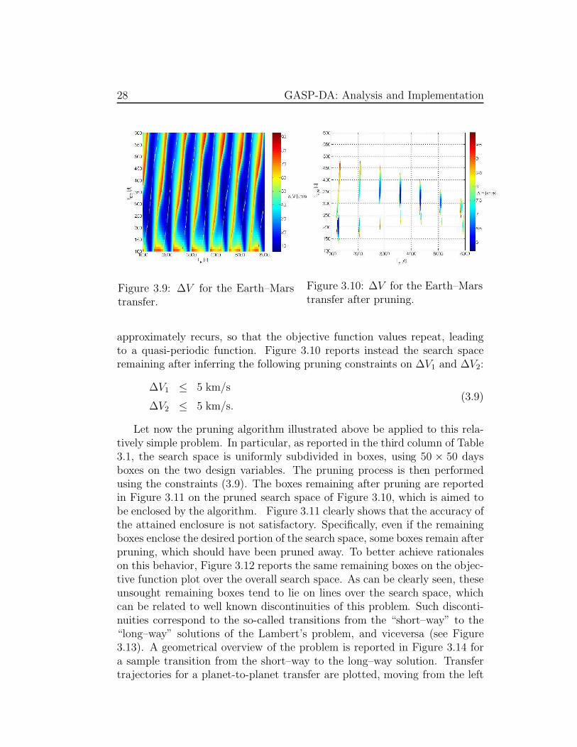
The previous algorithm has been implemented in COSY–Infinity and ap-plied to the Earth–Mars transfer. In particular, as summarized in Table 3.1,a search space of 5000 days on the departure epoch and 500 days on thetransfer time is selected. Figure 3.9 reports the overall !V over the definedsearch space. Quasi-periodicities can be identified on the figure, especiallyon the departure date, which can be easily related to the synodic period ofthe Earth–Mars system. In fact, based on the mean planetary orbital ra-dius and in the hypothesis of coplanar circular orbits, the synodical periodof the Earth-Mars system is assessed to be about 2.14 years, which can beclearly identified as the period of the oscillations in Figure 3.9. After onesynodical period, the relative geometrical configuration of Earth and Mars
variable lower bound upper bound amplitude units
TE 1000 6000 50 MJD
tEM 100 600 50 MJD
Table 3.1: Bounds and box-size for the design variables of the Earth–Marstransfer.
28 GASP-DA: Analysis and Implementation
Figure 3.9: !V for the Earth–Marstransfer.
Figure 3.10: !V for the Earth–Marstransfer after pruning.
approximately recurs, so that the objective function values repeat, leadingto a quasi-periodic function. Figure 3.10 reports instead the search spaceremaining after inferring the following pruning constraints on !V1 and !V2:
!V1 ! 5 km/s
!V2 ! 5 km/s.(3.9)
Let now the pruning algorithm illustrated above be applied to this rela-tively simple problem. In particular, as reported in the third column of Table3.1, the search space is uniformly subdivided in boxes, using 50 " 50 daysboxes on the two design variables. The pruning process is then performedusing the constraints (3.9). The boxes remaining after pruning are reportedin Figure 3.11 on the pruned search space of Figure 3.10, which is aimed tobe enclosed by the algorithm. Figure 3.11 clearly shows that the accuracy ofthe attained enclosure is not satisfactory. Specifically, even if the remainingboxes enclose the desired portion of the search space, some boxes remain afterpruning, which should have been pruned away. To better achieve rationaleson this behavior, Figure 3.12 reports the same remaining boxes on the objec-tive function plot over the overall search space. As can be clearly seen, theseunsought remaining boxes tend to lie on lines over the search space, whichcan be related to well known discontinuities of this problem. Such disconti-nuities correspond to the so-called transitions from the “short–way” to the“long–way” solutions of the Lambert’s problem, and viceversa (see Figure3.13). A geometrical overview of the problem is reported in Figure 3.14 fora sample transition from the short–way to the long–way solution. Transfertrajectories for a planet-to-planet transfer are plotted, moving from the left

3.2 The discontinuity problem 29
Figure 3.11: Enclosure of the prunedsearch space for the Earth–Marstransfer.
Figure 3.12: Boxes of Figure 3.11 re-ported on the overall search space ofthe Earth–Mars transfer.
Figure 3.13: Discontinuities on the !V for the Earth–Mars transfer.
side of the discontinuity to the right side. On the left side of the discontinuitythe short–way solutions are selected by the Lambert’s solver. Moving towardthe right side, the orbital plane inclination of the transfer trajectories tendsto increase. The discontinuity occurs when the transfer trajectory is exactlyperpendicular to the ecliptic. Just after the occurrence of the discontinuity,in order to keep dealing with prograde solutions of the Lambert’s problem,the long–way solution is suddenly selected. Corresponding to the previoustransition, a plot of the overall !V with respect to the departure epoch isreported in Figure 3.15: !V goes up close to the discontinuity, where the

30 GASP-DA: Analysis and Implementation
Figure 3.14: Geometrical overview ofthe transition from the short–way tothe long–way solution.
Figure 3.15: !V w.r.t. TE : transi-tion from the short–way to the long–way solution.
di"erence between the inclinations of the planetary orbital planes and ofthe transfer trajectory increases; a small discontinuity occur exactly at thepick, which can not be detected on the figure. Well known theoretical argu-ments show that Taylor polynomial expansions fail when discontinuities onthe processed function occur. This can be deemed the cause of the presenceof undesired boxes after pruning: Taylor expansions within boxes lying onthe discontinuity do not accurately approximate constraint functions; con-sequently bounds of the corresponding ranges are wrongly estimated, andthe boxes tend to be kept in the list of admissible solutions. Intensive workhas been devoted to overcome the discontinuity problem, and to improve theaccuracy of the enclosure of the pruned search space. A first attempt wasbased on the use of box-reshaping and box-splitting techniques, which arebriefly illustrated in section 3.2.1. The actual solution finally implementedin GASP–DA is instead illustrated in section 3.2.2.
3.2.1 Box-reshaping and box-splitting
A first attempt to solve the discontinuity problem is based on the observationthat the discontinuity lines tend to follow a straight path on the search space(see Figure 3.16). In particular, it can be easily assessed that, if Earth andMars followed circular and coplanar orbits, the discontinuity lines would beexactly straight line, with a common slope !, which could be related to theplanetary orbital periods by
tan! =PM
PE! 1, (3.10)

3.2 The discontinuity problem 31
!
Figure 3.16: The approximate slope of the discontinuities.
Figure 3.17: Sample box lying on thediscontinuity before reshaping.
Figure 3.18: Sample box after re-shaping.
where PM and PE are the orbital periods of Mars and Earth, respectively.
Based on the previous observation, boxes could be suitably reshaped inorder to reduce the number of boxes lying on the discontinuity, remainingafter the pruning process. Referring to Figure 3.17, suppose the reportedbox lying on the discontinuity is being processed. As already pointed out,the box is represented by the vector of DA numbers
[ !X] = {[TE ], [tEM ]} = {TE + "TE, tEM + "tEM}. (3.11)

32 GASP-DA: Analysis and Implementation
Figure 3.19: Enclosure of the pruned search space for the Earth–Mars transferusing reshaped boxes.
Using the approximate slope ! of equation (3.10), the new box
[ "X] = {TE + #TE + (1/ tan!) · #tEM , tEM + #tEM} (3.12)
can be gleaned out, which matches up the reshaping procedure depicted inFigure 3.18: two sides of the original box are made approximately parallelto the discontinuity line. As highlighted in the figure, the sample box wouldnot lie on the discontinuity after reshaping, so avoiding the problem of theassociated Taylor expansions.
As could be easily objected, the expedient of box-reshaping alone cannot solve the discontinuity problem, as boxes lying on the discontinuity linestill occur even after reshaping. This is illustrated in Figure 3.19, where thepruning algorithm is applied to the previous Earth–Mars transfer problemusing 50! 50 days reshaped boxes: even if the number of boxes lying on thediscontinuities decreases if compared with those of Figure 3.11, the accuracyof the enclosure of the pruned search space is still inadequate.
A box-splitting process has then been added to the previous reshapingtechnique, which is schematically presented in Figure 3.20 and 3.21. Supposethat, after reshaping, the box reported in Figure 3.20 is being processed. Thealgorithm for box-splitting is based on the following steps:
1. Moving on a horizontal line, passing through the center of the box (redline), identify a point lying on the discontinuity.

3.2 The discontinuity problem 33
Figure 3.20: Identification of thesplitting lines.
Figure 3.21: Reshaped boxes afterthe splitting procedure.
2. Enclose the discontinuity within a strip (magenta lines).
3. Identify two discontinuity-free boxes (see Figure 3.21).
4. Replace the original box with the two identified boxes.
Unfortunately, despite the simplicity and the theoretical e!ectiveness of thistechnique, some critical issues can be identified.
First of all, for the sake of computational time containment, the identifi-cation of the point lying on the discontinuity involved in step 1 is performedby processing the Taylor expansions of the related geometrical quantities.However, as already pointed out, Taylor expansions do not accurately rep-resent such quantities within these regions. Consequently, the identificationof the desired point turns out not to be accurate enough for the splittingpurposes.
Secondly, the definition of the enclosing strip of step 2 requires someheuristics for the suitable assessment of the width of the region to be ex-cluded. Evidently, the corresponding tolerances depend on the planetarysystem under study, since the deviation of the discontinuity lines from theapproximating straight line strongly depends on the planetary orbital ele-ments. A sharp enclosure of the discontinuity is however necessary, sincegood local minima and the global optimum lie close to the discontinuitiesfrom the short–way to the long–way solution of the Lambert’s problem inthis planet-to-planet transfer. Consequently, good regions are often thrownaway because of bad estimates of the tolerances.

34 GASP-DA: Analysis and Implementation
long wayshort way
Earth
Mars
Figure 3.22: The discontinuity fromthe short–way to the long–way solu-tion disappears in a planar model.
long wayshort way
Earth
Mars
Figure 3.23: The discontinuity fromthe long–way to the short–way solu-tion remains in a planar model.
Finally, a computational time increase follows. Besides the additional op-eration required by the previous algorithm, an evident cause can be detectedin step 4. Indeed, every box lying on the discontinuities is replaced by twoboxes, both of which must be processed again.
The previous considerations led to the decision of adopting the alternativestrategy to solve the problem, which is discussed in next section.
3.2.2 Planar planetary model
The implemented solution for the discontinuity problem is based on the ob-servation that the unfavorable discontinuity lines, i.e. the lines close to goodlocal minima, correspond to the transition from the short-way to the long-waysolution of the Lambert’s problem. The previous discontinuity do not occurif a planar planetary model is used instead of the actual three-dimensionalmodel associated to the ephemeris evaluator. This can be easily recognizedby analyzing again Figure 3.14. The discontinuity is related to the ambi-guity on the inclination of the orbital plane, when a perpendicular transferoccurs. In this situation, the definition of prograde and retrograde transfersis singular, and the inclination of the corresponding transfer orbit is charac-terized by sign ambiguity, i.e. ±90 deg. The previous ambiguity vanishes ifa planar planetary model is used: the orbital plane of the connecting Lam-bert’s arc is uniquely determined as coinciding with the ecliptic, and thetransition from the short–way to the long–way solution is continuous. It isworth observing that this is not the case for the transition from the long–way

3.2 The discontinuity problem 35
Figure 3.24: !V w.r.t. TE : transition from the short–way to the long–way so-lution. Comparison between the three-dimensional and the two-dimensionalplanetary models.
Figure 3.25: !V for the Earth–Marstransfer in the three-dimensionalplanetary model.
Figure 3.26: !V for the Earth–Marstransfer in the two-dimensional plan-etary model.
to the short–way solution (see Figure 3.22 and Figure 3.23): the ambiguityon the transfer plane vanishes, but a geometrical discontinuity remains. Thedisappearance of the first discontinuity is clearly confirmed in Figure 3.24,where the overall !V reported in Figure 3.15 is compared with the same plotin case the planar planetary model is used. Figures 3.25 and 3.26 address asimilar comparison, by plotting the !V over the whole search space in thetwo planetary models. The discontinuities corresponding to the transitionfrom the short-way to the long-way solutions disappear, whereas the other
36 GASP-DA: Analysis and Implementation
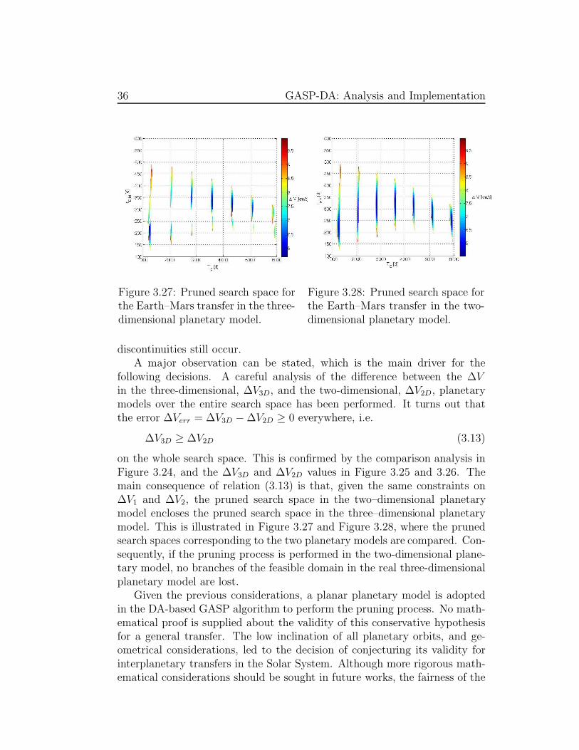
Figure 3.27: Pruned search space forthe Earth–Mars transfer in the three-dimensional planetary model.
Figure 3.28: Pruned search space forthe Earth–Mars transfer in the two-dimensional planetary model.
discontinuities still occur.A major observation can be stated, which is the main driver for the
following decisions. A careful analysis of the di!erence between the "Vin the three-dimensional, "V3D, and the two-dimensional, "V2D, planetarymodels over the entire search space has been performed. It turns out thatthe error "Verr = "V3D ! "V2D " 0 everywhere, i.e.
"V3D " "V2D (3.13)
on the whole search space. This is confirmed by the comparison analysis inFigure 3.24, and the "V3D and "V2D values in Figure 3.25 and 3.26. Themain consequence of relation (3.13) is that, given the same constraints on"V1 and "V2, the pruned search space in the two–dimensional planetarymodel encloses the pruned search space in the three–dimensional planetarymodel. This is illustrated in Figure 3.27 and Figure 3.28, where the prunedsearch spaces corresponding to the two planetary models are compared. Con-sequently, if the pruning process is performed in the two-dimensional plane-tary model, no branches of the feasible domain in the real three-dimensionalplanetary model are lost.
Given the previous considerations, a planar planetary model is adoptedin the DA-based GASP algorithm to perform the pruning process. No math-ematical proof is supplied about the validity of this conservative hypothesisfor a general transfer. The low inclination of all planetary orbits, and ge-ometrical considerations, led to the decision of conjecturing its validity forinterplanetary transfers in the Solar System. Although more rigorous math-ematical considerations should be sought in future works, the fairness of the

3.3 The dependency problem 37
Figure 3.29: GASP–DA on the two-dimensional model.
Figure 3.30: GASP–DA on the three-dimensional model.
hypothesis has been confirmed by the test phase illustrated in section 3.6:all the best-known solutions of typical MGA transfer problems have beenidentified to lie in the boxes remaining after the pruning process. It is worthanticipating that the previous approximation is only used within the pruningprocess, whereas the subsequent necessary optimization process is performedwithin the actual three-dimensional planetary model. As a further proof ofthe validity of the approximation, the performances of the pruning algorithmfor the case of the Earth–Mars transfer in the two–dimensional planetarymodel are analyzed in Figure 3.29 and Figure 3.30. The boxes remaining af-ter the pruning process sharply enclose the pruned search space of both thetwo-dimensional and the three-dimensional models. A plain improvement inthe enclosure accuracy can be detected in the three-dimensional model bycomparing Figure 3.30 with Figure 3.11.
3.3 The dependency problem
The previous considerations are based on analyses performed within theframework of a planet-to-planet transfer, i.e. an Earth-Mars transfer, wherethe departure epoch from Earth and the transfer time from Earth to Marsare selected as design variables. However, an alternative problem formula-tion is preferable. In particular, substituting the arrival epoch at Mars to thetransfer time from Earth to Mars in the set of the design variables has al-ready shown important advantages from a computational point of view [21].The use of this second formulation turns out to significantly reduce the num-ber of ephemeris evaluations required by the pruning algorithm, allowing the

38 GASP-DA: Analysis and Implementation
E
M
J
Figure 3.31: Scheme of an Earth–Mars–Jupiter transfer.
Figure 3.32: Design space for thefirst arc of the Earth–Mars–Jupitertransfer.
Figure 3.33: Design space for the sec-ond arc of the Earth–Mars–Jupitertransfer.
whole process to gain a polynomial complexity. Further reasons of selectingthis second formulation can be outlined, which are important alike for theDA-based GASP, especially if actual MGA transfers are studied.
Without loss of generality, consider the scheme of an Earth–Mars–Jupitertransfer, reported in Figure 3.31. The set of design variables usually selectedfor this MGA transfer is composed of the departure epoch from Earth, TE , thetransfer time from Earth to Mars, tEM , and the transfer time from Mars toJupiter, tMJ . For the sake of clarity, this formulation is referred to as “relativetimes formulation ” in the following. The evaluation of the overall !V willgenerally start from the analysis of the first connecting arc from Earth toMars. Suppose the relative times formulation is being used. Thus, referringto Figure 3.32, the quantities related to the first arc are characterized in theTE ! tEM plane. As both TE and tEM are design variables, in the framework

3.3 The dependency problem 39
of the DA-based GASP, a box is readily identified by the DA representationof both variables, and the computation goes on as depicted in the previoussections. Suppose now the first arc has been processed, and the second arcfrom Mars to Jupiter is of interest. The quantities associated to the secondarc are characterized in the TM ! tMJ plane, where TM is the arrival epoch atMars. However, TM is not a design variable in the relative times formulation,and it is computed as TM = TE + tEM . Even if tMJ is a design variable, thesize of the corresponding interval on TM is the sum of the box size on TE
and tEM in the DA-based GASP. The previous considerations can be easilyinferred to MGA transfers involving more than three planets: the box sizeof the departure epoch from each planet increases along the transfer. Thise!ect is strongly related to the dependencies associated to the relative timesformulation: the last departure epoch of an MGA transfer depends on all thedesign variables associated to the previous arcs, and the box size increasesaccordingly.
The dependency problem is better highlighted in Figure 3.34. Focusingon the dependence of the planetary ephemerides on the design variables, theposition of Earth, rE, depends only on the departure epoch TE. The posi-tion of Mars, rM , is evaluated using the epoch at Mars TM . Consequently,rM , will depend on the two variables TE and tEM . Similarly, the depen-dence of the position of Jupiter on the three variables TE , TM , and tEJ , ishighlighted. Thus, in a MGA transfer involving n planets, the position ofthe i-th planet will depend on the departure epoch from Earth, and all thetransfer times associated to the prior i ! 1 connecting arcs. Therefore, thedimensionality of the dependency increases along the transfer, reaching itsmaximum corresponding to the last connecting arc, where quantities, e.g. theplanet position, will depend on all n variables. Similar arguments hold forthe associated "V , on which inequality constraints are usually set.
The previous dependency problems can be overcome if the alternativestrategy suggested by Izzo et al. is used [21]. In particular, the departureepoch from Earth is kept within the set of design variables, whereas thetransfer times are now replaced by the epoch at each remaining planet of theMGA transfer. Referring again to the Earth–Mars–Jupiter transfer, the newset of variables will include the epochs at Earth, TE, Mars, TM , and Jupiter,TJ . In contrast to the relative times formulation, the new formulation isreferred to as the “absolute times formulation” in the following.
A review of the previous analyses will be of help to gain a valuable in-sight on the advantages of the new formulation. Consider again Figure 3.32and Figure 3.33. Using the absolute times formulation allows both arcs tobe characterized within planes that are directly defined by design variables.Thus, no box size increase occurs along the transfer. Referring instead to Fig-

40 GASP-DA: Analysis and Implementation
E
M
J
rJ
rE(TE)
rM (TE , tEM )
rJ(TE , tEM , tMJ)
Figure 3.34: Dependency problem for the Earth–Mars–Jupiter transfer.
ure 3.34, the planetary ephemerides will depend on the epoch of the planet,which is now included in the set of design variables. If the !V associated tothe whole transfer are of interest (which is the case in the pruning processof GASP), it can be easily shown that the maximum dimensionality of thedependency correspond to the !V of the powered gravity assist maneuvers,which will depend on three design variables.
The outcomes of the previous analysis led to the decision of adopting theabsolute time formulation as the baseline approach in GASP-DA. For the sakeof completeness, Figure 3.35 and Figure 3.36 report both the search spaceand the overall !V of the Earth–Mars transfer, which have been investigatedin Figure 3.9 and Figure 3.10, on the new plane TE ! TM .
3.4 Semi-analytical approximation
In the e"ort to further improve the algorithm performances in terms of com-putational time required by the pruning process, semi-analytical approachesto solve the implicit equations analyzed in section 3.1 have been investigated.The main idea is avoiding the iterative methods usually adopted for the so-lution of the implicit equations, i.e. Newton’s method, using either suitableexpansions of the equations or clever variable changes. The following sectionsare devoted to detail the techniques introduced for each equation.
3.4.1 Kepler’s equation
For the sake of clarity, Kepler’s equation 3.3 is reported again:
f(E) = E ! e sin E ! M = 0 (3.14)

3.4 Semi-analytical approximation 41
Figure 3.35: !V for the Earth–Marstransfer on the overall search spacein the TE ! TM plane.
Figure 3.36: !V for the Earth–Marstransfer on the pruned search spacein the TE ! TM plane.
This equation relates the planetary eccentricity, e, and mean anomaly, M ,which are readily available from the analytical ephemeris model, to the ec-centric anomaly E. An extensive analysis of this important equation canbe found in literature, and several methods have been developed to solve it.Among all the available methods, the semi-analytical techniques are deemedparticularly interesting for the current purpose. Battin [2] illustrates howa useful solution of equation (3.14) can be obtained by expanding it withrespect to the eccentricity e. Such kind of solution turns out to be partic-ularly appropriate in the framework of the ephemeris evaluation, since allthe planetary orbits in the Solar System are characterized by relatively loweccentricity values. Consequently, a third order expansion of equation (3.14)is used to gain the explicit relation for E
E " M +e sin M
1 ! e cosM!
1
2
!
e sin M
1 ! e sin M
"3
. (3.15)
The computed eccentric anomaly E is then used to evaluate planetarypositions and velocities, through classical algebraic manipulations. Figure3.37 and Figure 3.38 investigate the error of the semi-analytical approachwith respect to the iterative process of a classical Newton’s method. Inparticular, referring to a sample interval epoch of one Martian year, Figure3.37 reports the di"erence between the position vectors resulting from thetwo approaches on the x!y plane. The maximum error is of the order of 1000km. A similar analysis is addressed in Figure 3.38 for the velocity vector,where a maximum error of the order of 0.1 m/s is detected. This error isacceptable, even though the orbital eccentricity of Mars is not negligible.

42 GASP-DA: Analysis and Implementation
Figure 3.37: Position error of thesemi-analytical solution of Kepler’sequation w.r.t. Newton’s method.
Figure 3.38: Velocity error of thesemi-analytical solution of Kepler’sequation w.r.t. Newton’s method.
3.4.2 Lagrange’s equation
The !V evaluation requires the solution of the Lambert’s problem. As al-ready pointed out in section 3.1, the Lagrange’s equation for the time offlight,
f(x) = A(x) ! t = 0, (3.16)
must be solved, where (see [2] for details)
A(x) = a(x)3/2((!(x) ! sin(!(x))) ! ("(x))). (3.17)
The functions ! and " are related to x via the relations
sin2 1
2! =
s
2asin2 1
2" =
s ! c
2a, (3.18)
where s and c are geometrical parameters defined in [2], and a is the semi-major axis of the resulting conic arc. The semimajor axis is a direct functionof x:
a =s
2(1 ! x2). (3.19)
As suggested by Izzo, equation (3.16) can be suitably manipulated to improvethe convergence performances of the iterative algorithms. In particular, thesolution of the equation
f = log A(x) ! log t = 0 (3.20)

3.4 Semi-analytical approximation 43
is sough, which replaces the original equation. Moreover, the following vari-able change is adopted:
x = log (1 + x) . (3.21)
Using the new variable x, the curve associated to equation (3.20) is wellapproximated by a straight line. Consequently, a first order expansion of theequation can be used to approximate the solution. In particular, the solutionis then approximated by
x = x0 !f(x0)
f !(x0), (3.22)
where f !(x0) is computed analytically. The heuristics for the selection of thereference point x0 is based on the identification of a circular orbit, whoseangular velocity is equal to the mean angular velocity of the spacecraft onthe actual connecting arc. More specifically, the transfer time t, as well asthe angle between the initial and final position vectors !!, are input to theLambert’s solver. The radius R0 of a circular orbit is sough, which solves theequation
!
µ
R30
t = !!. (3.23)
The radius R0 is then used to compute the reference point x0 through therelations (3.19) and (3.21).
Once the solution x of equation (3.20) is obtained, the solution of theoriginal equation (3.16) can be readily computed using again the previousrelations. Figure 3.39 reports the overall !V for the Earth–Mars transfer,which is compared with the same !V resulting from the semi-analytical so-lutions of both Kepler’s and Lagrange’s equations, reported in Figure 3.40.Once again, it is worth anticipating that all the semi-analytical approxima-tions here introduced are only used within the pruning phase of the overalloptimization process.
3.4.3 Bending angle equation
As described in section 3.1, in the framework of MGA transfers, the planeto-centric trajectories at the gravity assists are made by two arcs of hyperbolapatched together. Within the powered gravity assist model, the pericenterof the hyperbola is evaluated by solving the implicit equation
f(rp) = arcsina"
a" + rp+ arcsin
a+
a+ + rp! " = 0 (3.24)

44 GASP-DA: Analysis and Implementation
Figure 3.39: !V for the Earth–Marstransfer.
Figure 3.40: !V for the Earth–Marstransfer: semi-analytical approach.
where a! = 1/(vin" · vin
") and a+ = 1/(vout" · vout
" ). Similarly to the previouscase, a suitable variable change is looked for to allow equation (3.24) to bewell approximated by a linear expansion. The variable change
x = 1/rp (3.25)
has been identified to properly serve this purpose. Once again, using the newvariable x, the first order expansion of the equation is used to approximatethe solution by
x = x0 !f(x0)
f #(x0), (3.26)
where f #(x0) is computed analytically. The reference point x0 is chosen usinginformation associated to both incoming and outgoing hyperbola. In partic-ular, the incoming and outgoing hyperbolic arcs are processed separately tocompute the corresponding pericenter radii, which make the spacecraft spanthe whole bending angle !, without any !V corrections at the pericenter.The two radii are then averaged to obtain the mean radius
rp0 =a!(b ! 1) + a+(b ! 1)
2, (3.27)
where b = 1/sin(!/2). The reference point x0 is then computed throughrelation 3.25 using the radius rp0. Once the solution x of equation f(x) = 0 isavailable, the actual pericenter radius of the powered gravity assist maneuvercan be computed using again equation 3.25.

3.4 Semi-analytical approximation 45
Figure 3.41: Bending angle equation: error of the semi-analytical approxima-tion w.r.t. Newton’s method corresponding to random gravity assist samples.
The accuracy of this semi-analytical approximation is investigated in Fig-ure 3.41. Gravity assist samples are generated by randomly selecting valuesof !, vout
! , and vin! within the ranges
vout! , vin
! ! [6, 40] km/s
! ! [0, 60] deg.(3.28)
For each sample, the corrective !V within the powered gravity assist modelis computed by solving equation (3.24), using both Newton’s method and theprevious semi-analytical approach. The relative error is then plotted for eachsample. The maximum relative error is about 3.5%, even if most samples arecharacterized by an error less than 0.1%. This is confirmed even in morecomplex MGA transfers. For example, the overall !V of the best-knownCassini–like transfer reported in section 3.6 is
!V = 4.930710687853622 km/s. (3.29)
Using the semi-analytical approach, the same evaluation yields
!V = 4.931949452024911 km/s, (3.30)
matching a relative error of 0.025%.

46 GASP-DA: Analysis and Implementation
bounds
validated
X[X]
Figure 3.42: Validated bounds basedon LDB.
non ! validated
bounds
X[X]
Figure 3.43: Non–validated boundsbased on the quadratic bounder.
3.5 Quadratic polynomial bounder
As already pointed out, the Linear Dominated Bounder (LDB) has been usedto estimate the range of the constraint functions over each box in the pruningprocesses of the previous examples. The LDB algorithm was introduced byBerz and Makino [26] in the framework of Taylor Models, which can beconsidered as the result of a joining process between di!erential algebraictechniques and interval analysis [29], aimed at performing computer–assistedvalidated computations (see chapter 6). Without loss of generality, supposea polynomial of one variable has to be bounded within an interval I. LDB isbased on the observation that, if d is the width of the domain interval, thenthe widths of the Ik are expected to scale as
width(Ik) ! dk. (3.31)
Hence, the dominating part of the total bounds of a polynomial are expectedto come from the linear part. A rigorous enclosure of the range is thenobtained by suitably derived methods to bound higher order parts.
However, a careful analysis of the pruning process in MGA transfers hasshown that polynomial bounding based on LDB is not as e!ective as desired.The reason of such behavior is schematically described in Figure 3.42. Withinthe pruning process, suppose a box [X] can be pruned away if
min[X]
f > fcutoff , (3.32)
where f is the constraint function under analysis, and fcutoff is its maxi-mum allowed value. The validated LDB uses the linear part of the Taylor

3.6 Test cases 47
expansion of f around a reference point to get rigorous bounds of the Taylorexpansion. Unfortunately, due to accuracy problems on the bounding processof nonlinear terms, the resulting interval enclosure overestimates the exactrange. If LDB were used in the example of Figure 3.42, the box [X] wouldnot be pruned away, even if evidently satisfying inequality (3.32). This over-estimation problem leads to ine!ective pruning processes, and more boxesremain after pruning than expected from classical GASP results.
In order to overcome the previous di"culty, a non–validated quadraticbounder has been implemented, which uses the quadratic part of the Tay-lor expansion to get non–validated interval enclosures of the range of f over[X]. The process is illustrated in Figure 3.43. Second order information areadded to the previous analysis. If the resulting quadratic polynomial turnsout to be positive defined, its minimum is easily estimated by locating thezero–gradient point, and checking its inclusion within [X]. Only linear infor-mation are kept to estimate the minimum in case of lack of positive defini-tion properties. In the example of Figure 3.43, the introduced non–validatedbounder would correctly prune away the box. An evident drawback is that,in contrast to the validated LDB, the non–validated quadratic bounder couldunderestimate the exact interval enclosure. However, an extensive test phaseconfirmed the validity of the introduced approximations: using the resultingDA–based GASP algorithm, the best solutions available in literature for ev-ery test case reported in section 3.6 turn out to lie in the boxes remainingafter pruning. This result is confirmed in Figure 3.44 and Figure 3.45, wherethe performances of GASP-DA are illustrated for the Earth–Mars transfer:the remaining boxes accurately enclose the pruned search space.
3.6 Test cases
In this section, significant test cases are addressed to properly assess theperformances of the resulting DA–based GASP algorithm. Before reportingthe results of the test phase, section 3.6.1 describes the philosophy adoptedfor the optimization process following the GASP-DA pruning process, whichis evidently necessary to serve the purpose of optimizing the overall #V . Testcases are then reported, ordered by increasing complexity. In particular,relatively simple planet-to-planet transfers are addressed in sections from3.6.2 to 3.6.4. MGA transfers involving three (sections 3.6.5 and 3.6.6), andfour (section 3.6.7) planets follow. Finally, a Cassini–like transfer is optimizedin section 3.6.8. The structure of each transfer is fixed and specified a prioriin all test cases, i.e. the planets sequence of each transfer is fixed, thus notincluded in the set of design variables.

48 GASP-DA: Analysis and Implementation
Figure 3.44: Performances of thenon–validated quadratic bounder onthe Earth–Mars transfer problem.
Figure 3.45: Performances of thenon–validated quadratic bounder:detail of Figure 3.44.
For each test, the problem is first defined. The search space is identified bylower and upper bounds on each variable. Referring to the box-wise approachof GASP–DA, the size of the sampling box corresponding to each variableis reported. The cuto! values set for the departure and arrival "V , as wellas for the corrective "V at each gravity assist are indicated. Pertaininginstead the minimum allowed pericenter radii for the powered gravity assistmaneuvers, a common philosophy has been adopted for all planets: giventhe mean radius of the generic planet P , RP , the corresponding minimumallowed pericenter radius is set to 1.05 RP .
Thus, the results of the pruning process are reported in terms of the totalnumber of boxes, the number of feasible boxes remaining after pruning, andthe CPU time required by the pruning process. It is worth observing that thetotal number of boxes is meant to give an idea on the dimension of the searchspace, and it is di!erent from the number of processed boxes. The computa-tional time is relative to a PC, 1.9 GHz CPU, 512 Mb RAM. Second orderexpansions are used in all test cases. As far as the subsequent optimizationprocess is concerned, the best identified "V is reported, together with a plotof the corresponding optimal transfer. The values of the minimum pericenterradii considered for the GA throughout the report are given in Table 3.2.
Table 3.2: Minimum pericenter radii.
V E M J S
rpmin[km] 6353.55 6689.55 3558.45 73406.55 61143.36

3.6 Test cases 49
3.6.1 The optimization process
The outcome of the pruning process carried out by GASP–DA is a list ofboxes, all fulfilling the requirement that a portion of them at least satisfies thefeasibility conditions related to the constraining !V values and the minimumallowed pericenter values. An optimization process is then necessary to locatethe minimum of the objective function, which is the purpose of the originaloptimization problem. This section is dedicated to the description of thephilosophy adopted for this optimization phase.
Two approaches have been studied. The first approach is based on theuse of the validated global optimizer COSY–GO, that is a branch-and-boundoptimization algorithm, which takes advantage of Taylor models to boundthe objective function value over the processed boxes [15]. Further detailson COSY–GO can be found in chapter 6. Unfortunately, some general draw-backs can be identified which led to the decision of avoiding its use. First ofall, the current version of COSY–GO can not manage constraints explicitly,which forces to either implement tailored techniques to handle constraints orto add them to the objective function as penalty terms. Moreover, due tothe lack of the embedded possibility of exploiting the cascade structure ofthe MGA transfer problem, the computational time exponentially increaseswith the dimensionality.
The previous considerations have been of main influence for the decisionof utilizing other approaches. In particular, multiple runs of a local optimizerhave been exploited. The philosophy is based on the following steps:
1. The non–validated bounding process described in section 3.5 returnsestimates of the minimum of the objective function, including its loca-tion, within each box.
2. The boxes are sorted based on the minimum objective function valuesestimated in step 1.
3. A certain number of boxes are suitable selected.
4. Starting from the estimated location of the minimum, a local optimiza-tion run is performed within each selected box.
The introduced optimization philosophy worths some comments. As al-ready anticipated in the previous sections, di"erent models and methods forthe constraint and objective functions evaluation are implemented in the twomain phases of the previous algorithm, i.e. search space pruning and total !Voptimization. In particular, the planar Solar System model, and the semi–analytical approaches to the solution of the implicit equations are used within

50 GASP-DA: Analysis and Implementation
Figure 3.46: Heuristics for box selection.
the search space pruning phase only. This decision relies on the conserva-tive hypothesis pertaining the planetary model depicted in section 3.2.2, andon the observation that the semi–analytical approaches deliver su!cientlyaccurate solutions of the implicit equations. The previous approximationsare all abandoned in the subsequent optimization process of step 4, wherethe actual three-dimensional Solar System model, and the iterative Newton’smethod are used to evaluate the planetary ephemerides and to compute thesolutions of the implicit equations.
Moreover, the boxes selection phase (step 3) is based on the followingheuristics. Referring to Figure 3.46, suppose the overall objective functionrange is available, which is computed on all the minima identified withineach box in step 1. The interval corresponding to 5% of the overall range isevaluated. The boxes whose estimated local minimum belongs to this intervalare selected for the subsequent analyses. The 5% value is purely based onthe experience gained during the extensive test phases. The parameter isanyway kept settable by the user.
The local optimization processes involved in step 4 are carried out withineach box. This means that the identified local minima are interior to the fea-sible boxes, as well as the finally estimated global minimum. Consequently,if a minimum is identified to coincide with the best known solution availablein literature, this turns out to lie in the boxes remaining after the prun-ing process based on GASP–DA. The local optimization processes are per-formed using the Matlab function “fmincon”, which implements a sequentialquadratic programming algorithm. No particular motivations underlie theselection of fmincon, which was mainly driven by the availability of interfacetools between COSY-INFINITY and Matlab.

3.6 Test cases 51
3.6.2 EM
Table 3.3: Search space and best identified solution for the EM transfer.
planet variable lower bound upper bound size cuto! (10) solution[days] [days] [days] [km/s] [days]
E TE 1000 6000 50 5 3573.188M tEM 100 600 50 5 324.047
The first test case is the Earth–Mars transfer. The search space is definedin Table 3.3. It is worth observing that bounds on the departure epoch fromEarth, TE , and on the transfer time from Earth to Mars, tEM are given.Consequently, the search space definition is made within the relative timesformulation. However, as stated in section 3.3, the pruning processes arecarried out in the absolute times formulation. This observation holds forall the following test cases. The box size along each epoch is indicated inthe fifth column. The cuto! values for the maximum allowed departure andarrival "V are reported in the last column. A further constraint is imposedto the maximum allowed overall "V , which is reported within round bracketson the head row.
The main results pertaining the performances of GASP–DA are summa-
Figure 3.47: Trajectory of the best identified EM transfer.

52 GASP-DA: Analysis and Implementation
rized in the following:
• Total number of boxes: 1000
• Feasible boxes: 64 (6.4%)
• CPU time: 0.220 s
• Best identified !V : 5.6673 km/s
The reported value of the best identified !V refers to the results of theoptimization process described in section 3.6.1, which follows the pruningprocess of GASP–DA. The last column of Table 3.3 lists the values of thedesign variables corresponding to the best identified solution, whereas Figure3.47 reports a two–dimensional plot of the related trajectory.
3.6.3 EV
Table 3.4: Search space and best identified solution for the EV transfer.
planet variable lower bound upper bound size cuto" (10) solution[days] [days] [days] [km/s] [days]
E TE 1000 6000 50 5 2706.421
V tEV 100 500 50 5 151.754
A further planet-to-planet transfer test case is here analyzed, selectingVenus as the arrival planet. Similarly to the previous case, the search spaceand the main parameters are defined in Table 3.4. The cuto" values for themaximum allowed departure and arrival !V are reported in the last column,and a further constraint of 10 km/s is added to the overall !V .
The main results pertaining the performances of GASP–DA are summa-rized in the following:
• Total number of boxes: 800
• Feasible boxes: 78 (9.7%)
• CPU time: 0.492 s
• Best identified !V : 6.0638 km/s
Figure 3.48 reports a two–dimensional plot of the best identified trajectory,whose solution vector is stated in the last column of Table 3.4.

3.6 Test cases 53
Figure 3.48: Trajectory of the best identified EV transfer.
3.6.4 EJ
Table 3.5: Search space and best identified solution for the EJ transfer.
planet variable lower bound upper bound size cuto! (16) solution[days] [days] [days] [km/s] [days]
E TE 1000 10000 50 8 6198.093J tEJ 100 5000 100 8 1097.004
A last planet-to-planet transfer test case is here addressed. Jupiter isnow the arrival planet, and the search space, together with the main algo-rithm settings, are defined in Table 3.5. A much larger launch window isconsidered in this case to better highlight the performances of the algorithmin terms of computational time, through comparison with the previous testcases. It is worth observing that a larger box size is used for TJ : the greaterorbital period and the slower dynamics associated to the outer regions of theSolar System allows the user to select a wider sampling interval on the corre-sponding design variables, without significant loss of accuracy. A maximumallowed overall "V of 16 km/s is used as overall cuto! value.
Again, the main results pertaining the performances of GASP–DA aresummarized in the following:

54 GASP-DA: Analysis and Implementation
Figure 3.49: Trajectory of the best identified EJ transfer.
• Total number of boxes: 8820
• Feasible boxes: 46 (1.0%)
• CPU time: 2.116 s
• Best identified !V : 14.4197 km/s
The best solution found is identified by the values of the design variablesreported in Table 3.5. Figure 3.49 illustrates a two–dimensional plot of thecorresponding trajectory.
3.6.5 EVM
Table 3.6: Search space and best identified solution for the EVM transfer.
planet variable lower bound upper bound size cuto" (12) solution[days] [days] [days] [km/s] [days]
E TE 1000 6000 50 5 5611.480
V tEV 100 500 50 2 157.603M tV M 100 1000 50 5 255.596

3.6 Test cases 55
The study of actual MGA transfer starts from this section. In particu-lar, one planet is added to the planets sequence, where a powered gravityassist maneuver is performed. In particular, an Earth–Venus–Mars transferis investigated. The search space is defined in Table 3.6. Whereas the cuto!values at Earth and Mars are still related to the departure and arrival "V ,the cuto! value of 2 km/s at Venus now refers to the maximum allowed cor-rective "V at the pericenter of the corresponding hyperbolic trajectory, asprovided by the powered gravity assist model.
The main performance parameters are reported in the following, whereasthe last column of Table 3.6 reports the optimal solution identified at theend of the pruning and optimization processes. A two-dimensional plot ofthe corresponding trajectory can be found in Figure 3.50.
• Total number of boxes: 14400
• Feasible boxes: 165 (1.1%)
• CPU time: 1.8321 s
• Best identified "V : 8.5226 km/s
Figure 3.50: Trajectory of the best identified EVM transfer.
Although the total number of boxes is greater than in the previous test case,the required CPU time for the search space pruning turns out to be lower.This might be deemed a!ecting the correctness of the results. However, as

56 GASP-DA: Analysis and Implementation
already pointed out, the reader must notice that the total number of boxesdoes not coincide with the number of boxes actually processed by GASP–DA,thanks to forward and backward constraining of GASP scheme [21].
3.6.6 EMJ
Table 3.7: Search space and best identified solution for the EMJ transfer.
planet variable lower bound upper bound size cuto! (20) solution[days] [days] [days] [km/s] [days]
E TE 1000 6000 50 10 3543.787
M tEM 100 1200 50 5 1121.130J tMJ 100 2000 100 10 1109.307
A further MGA transfer involving three planets is investigated in thissection. In particular, after departure from Earth, a powered gravity assistis performed at Mars before the arrival at Jupiter. The search space ofthe resulting Earth–Mars–Jupiter transfer is defined in Table 3.7. Cuto!values of 10, 5, and 10 km/s respectively are used at each planet, whereas amaximum value of 20 km/s constraints the overall "V .
Figure 3.51: Trajectory of the best identified EMJ transfer.
The performances of GASP–DA are analyzed in the following:

3.6 Test cases 57
• Total number of boxes: 41800
• Feasible boxes: 329 (0.7%)
• CPU time: 2.640 s
• Best identified !V : 13.4165 km/s
Figure 3.51 plots the trajectory corresponding to the lowest !V found, whosesolution vector is reported in Table 3.7.
3.6.7 EVME
Table 3.8: Search space and best identified solution for the EVME transfer.
planet variable lower bound upper bound size cuto" (15) solution
[days] [days] [days] [km/s] [days]
E TE 3000 4000 50 6 3985.096V tEV 25 525 50 2 160.500
M tV M 20 520 50 2 168.941E tME 25 525 50 6 301.615
Two gravity assists are here introduced for an Earth–Venus–Mars–Earthtransfer. Four planets are then involved, so leading to a four-dimensionaloptimization problem. The search space of this EVME transfer is defined inTable 3.8. A maximum value of 15 km/s is allowed for the overall !V .
The main results pertaining the performances of GASP–DA are summa-rized in the following, whereas Figure 3.52 reports a two-dimensional plotof the trajectory corresponding to the best identified solution. The relatedsolution vector is supplied in Table 3.8.
• Total number of boxes: 20000
• Feasible boxes: 26 (0.1%)
• CPU time: 0.2 s
• Best identified !V : 12.4431 km/s

58 GASP-DA: Analysis and Implementation
Figure 3.52: Trajectory of the best identified EVME transfer.
3.6.8 EVVEJS
This section is devoted to a complex MGA transfer problem, which has beenalready analyzed in the past [21, 16]. The arrival planet Saturn is reachedafter four gravity assists. Thus, the overall transfer involves six planets, soleading to a six-dimensional optimization problem. The sequence is fixed toEarth–Venus–Venus–Earth–Jupiter–Saturn. The previous sequence can beclearly related to the sequence of the Cassini mission, except no deep spacemaneuvers are allowed, whose introduction will be considered in the nextchapter. Before presenting the results for this test case, some notes mustbe reported about a further necessary expedient which had to be added incase of MGA transfers where resonances might play an important role in theoptimization, as in the case of the EVVEJS transfer.
As already pointed out in section 3.2, the discontinuity problem has beensolved by adopting a planar planetary model. This expedient eliminates thediscontinuities related to the transition from the short–way to the long–waysolution of the Lambert’s problem. Nevertheless, it is not able to solve thesame problem for the related transition from the long–way to the “short way”solution. Consider the Venus–Venus arc of an EVVEJS transfer. Figure 3.53shows that, when the angle between the first and second Venus encounter isclose but less than 2!, the long way solution is selected. However, consideringthe same transfer time, the features of the resulting transfer suddenly changejust after passing the angle 2!, which discriminates between the short–way

3.6 Test cases 59
long wayshort way
Venus
1 22
Figure 3.53: Venus–Venus arc: long–way to short–way solution.
long way
Venus
multi-revolution
1 22
Figure 3.54: Venus–Venus arc:multi–revolution solution.
and the long–way solutions. The occurrence of this discontinuity is particu-larly undesirable in such kind of arcs, where resonance conditions are knownto improve the overall transfer performances. The resonance occurs when thepositions of the first and second planet encounter coincide. Consequently, ifTP indicates the orbital period of planet P , the transfer time associated tothe connecting arc must satisfy
tV V = r TV , (3.33)
where r is a positive integer number, r ! 2. The presence of the previousdiscontinuity strongly a!ects the performances of the pruning algorithm: asthe center of the box is used to discriminate between the two Lambert’sproblem solutions, boxes containing resonance situations will turn out to beobviously pruned away if the center of the box, which is the reference pointfor the Taylor expansions, corresponds to the short–way solution of Figure3.53.
An expedient is used to overcome the previous di"culties, which is basedon the observation that, in a planet-to-planet transfer involving only oneplanet, the discontinuity disappears if multi-revolution solutions are allowed(see Figure 3.54). In particular, given a box to be processed, is the enclosedtransfer times include the resonance condition (3.33), and the enclosed anglesbetween the first and second encounter include the resonance angle 2!, themulti–revolution solution is allowed. In this manner, the EVVEJS test casecan be e!ectively managed by GASP–DA, as illustrated in the following test.The search space for the corresponding optimization problem is set as definedin Table 3.9. A maximum value of 12 km/s is used for the overall #V .
The main results pertaining the performances of GASP–DA are summa-rized in the following:

60 GASP-DA: Analysis and Implementation
Table 3.9: Search space and best identified solution for the EVVEJS transfer.
planet variable lower bound upper bound size cuto! (12) solution[days] [days] [days] [km/s] [days]
E TE -1000 0 50 4 -790.605
V tEV 10 410 25 2 159.962V tV V 100 500 25 2 449.386E tV E 10 410 25 2 54.171J tEJ 400 2000 200 2 1029.979S tJS 1000 6000 200 6 4560.625
Figure 3.55: Trajectory of the bestidentified EVVEJS transfer.
Figure 3.56: EVVEJS transfer: de-tail of Figure 3.55.
• Total number of boxes: 32768000
• Feasible boxes: 1085 (0.003%)
• CPU time: 1.93 s
• Best identified "V : 4.9357 km/s
Note that the best identified "V refers to the final insertion of the spacecraftinto an orbit around Saturn of eccentricity 0.98 and periapsis 108950 km,as considered in [21]. Figure 3.55 reports a two–dimensional plot of thetrajectory corresponding to the best identified solution, whose solution vectoris listed in Table 3.9. The identified solution turns out to be characterizedby an objective function value which is slightly higher than the known bestsolution in literature [32]. Further analyses are necessary to identify the

3.7 Final remarks 61
reason of such discrepancy, which is deemed to be related to di!erences onthe minimum allowed pericenter radii at each gravity assist.
3.7 Final remarks
The introduction of DA techniques into GASP algorithm has been addressedin this chapter. The main idea was dealing with Taylor expansions of theconstraint and objective functions over boxes that sample the search space,instead of handling point–wise evaluations as performed in the original GASPalgorithm. This turned out to pose some significant challenges. First ofall, the expansion of the solution of parametric implicit equations had tobe achieved. Moreover, proper modeling decisions had to be taken, dueto the presence of discontinuities on the constraint and objective functions.The resulting GASP–DA algorithm turned out to perform considerably wellin typical test cases. This result is also the outcome of further importantarguments, which led to the implementation of semi–analytical approaches tosolve the implicit equations involved in the constraint and objective functionevaluation, and to the development of a non–validated quadratic bounder.However, the planets sequence is kept fixed and specified a priori, whichrepresents a key point for the future development of an e!ective MGA transferoptimizer.

62 GASP-DA: Analysis and Implementation

Chapter 4
Introduction of DSM inGASP-DA
The GASP-DA algorithm, extensively discussed in the previous chapter, isnow modified to manage DSM. These maneuvers are usually carried out toimprove the performances of the transfer trajectories in terms of total cost.From the trajectory optimization standpoint, each DSM involves additionaldegrees of freedom that widen the search space and increase the chances offinding better global optima than those associated with pure MGA trajecto-ries. The mathematical formulation of this new problem is not unique, andthe final result is strongly a!ected by the problem transcription, especiallywhen working in a DA frame. In this chapter we consider two di!erent for-mulations of the MGA-DSM problem. We choose the strategy that betterfits the GASP-DA algorithm already developed. In particular, we implementthe GASP-DSM-DA algorithm that prunes the search space associated tothe DSM variables beside that associated to the MGA ones (epochs).
In section 4.1 we make some preliminary considerations and point outthe problems associated to the DSM introduction. Two di!erent strategiesfor the problem formulation are deeply analyzed in sections 4.2 and 4.3.In particular, in both frameworks, the dependence of the functions on theproblem variables is studied for both a planet-to-planet and a MGA case.The strategy that better fits the DA implementation is introduced in GASP-DA to produce the GASP-DSM-DA algorithm (section 4.4). This algorithmis tested for the solution of some sample cases discussed in section 4.5. Finalconsiderations are made in section 4.6.

64 Introduction of DSM in GASP-DA
4.1 Preliminary Considerations
In a MGA problem, the transfer trajectory is made up by a number of Lam-bert’s arcs linked together in proximity of the planets. In this framework,the objective function evaluation consists in the solution of a set of Lam-bert’s problems with the positions of two consecutive planets as inputs. Thisinformation can be extracted once the epochs of the planets encounters arespecified, and therefore the decision vector of a MGA problem consists in acollection of epochs.
In a MGA-DSM problem, the objective function evaluation consists inthe solution of several Lambert’s problems (between two consecutive planetsor, depending on the problem structure, between a planet and a maneuverpoint, and vice versa).The location of the maneuver points has to be specifiedby appending new variables to the decision vector. It can be easily shownthat, for each DSM introduced, the minimum number of additional variablesis four in the 3D case and three in the 2D case. For the same reasonsdiscussed in the previous chapter, in this study, the search space pruning ofMGA-DSM transfers is carried out in the 2D space, whereas the subsequentoptimization deals with the full 3D space. This means that, letting nP and nD
be the number of planets and the number of DSM of a MGA-DSM transfer,respectively, the decision vector for the search space pruning, in our case, ismade up by nP + 3nD variables.
One of the purposes of this study is the implementation and the assess-ment of the search space pruning (of both MGA and MGA-DSM problems)exploiting the DA formalism. In particular, the pruning process relies on in-equality constraints, as the magnitude of the !v maneuvers and the closestdistance to a planet, usually expressed as nonlinear functions of the deci-sion vector. Analogously to the MGA case, the pruning process of MGA-DSM problems consists in: 1) representing these nonlinear functions, overappropriate subsets (boxes) of the search space, as Taylor polynomials ofthe decision variables; 2) bounding these functions using suitable bounders;3) pruning away unfeasible boxes from the search space. Di"erently from apoint-wise approach, the whole procedure is based on the reliability of thebounding process and, in order to e#ciently prune the search space, workingwith smooth functions of as few variables as possible is crucial. This meansthat, in specifying the DSM point, di"erent strategies generate functions hav-ing di"erent dependencies from the decision variables, and so the outcome ofthe pruning process, in a DA frame, is di"erent. This is the key that has tobe taken into account for the strategy selection.
Another consideration concerns the increased computational burden whenmoving from the MGA to the MGA-DSM problem. This is not only related

4.1 Preliminary Considerations 65
P1(T1)
P2(T2)!v1
!v2
Figure 4.1: A planet-to-planet transfer.
to the increased dimension of the search space (from nP to nP + 3nD), butrather it is an intrinsic consequence of representing a function with its Taylorexpansion. The number of monomials needed to represent a function of vvariables up to the order n is NM = (n+v)!/(n!v!). This means that, even ifthe order is kept constant, the number of monomials necessary to deal witha MGA-DSM problem increases with factorial law if compared to a simpleMGA problem. These monomials should be stored along the entire pruningprocess, and consequently the 3nD additional variables strongly a!ect thealgorithm performances. In particular, the time for the algorithm executionincreases since a larger amount of memory has to be allocated and a greaternumber of operations is required.
The bottom line is that, in general, the complexity of a MGA-DSM prob-lem increases if compared to a standard MGA problem. This complexity canbe circumscribed by carefully selecting the strategy for the representation ofthe maneuver point. In particular, it is important to preserve the idea of theGASP algorithm: subdivide the problem into a cascade of subproblems andexploit the cut-o! values to prune away unfeasible zones.
Let us briefly recall the statement of a planet-to-planet problem (Figure4.1). In this simple problem, the transfer from P1 to P2 is considered. Thetwo epochs, departure and arrival, are denoted with T1 and T2, respectively.The decision vector is then x = [T1, T2]. The objective function is evaluatedby solving one Lambert’s problem. The pruning process consists in findingthe feasible subset of the search space, X , such that
"v1(x!) ! "vmax
1 , "v2(x!) ! "vmax
2 , "x! # X . (4.1)
The size of the departure and arrival maneuvers is denoted by "v1 and "v2,respectively; the two corresponding cut-o! values are "vmax
1 and "vmax2 .

66 Introduction of DSM in GASP-DA
4.2 Forward Propagation Strategy
In this section we show the first devised strategy for the formulation of theMGA-DSM problem. In the forward propagation method, the location ofthe maneuver point is a function of all the variables involved in transfer upto the point considered. As it will be shown, this procedure intrinsicallyexploits some problem constraints but gives rise to functions depending onmany number of variables. We show this technique, and the associated setof 3nD additional variables, by means of two examples: a planet-to-planettransfer (with one DSM) and a MGA transfer (three planets and two DSM).
4.2.1 Planet-to-Planet Case
Let us consider the problem illustrated in Figure 4.2. A deep space maneuver,located at the point D, is performed in the transfer between the two planetsP1 and P2. In order to specify the maneuver point, we introduce two angles
! – flight-path angle: is the angle between the velocity of P1, v1, and thevector !v1;
" – incremental anomaly : is the anomaly of the point D relative to P1.
The departure velocity, v!, can be computed once both ! and !v are assigned,i.e. v! = v!(v1, !, !v1). The location of D can be determined by forwardpropagating, using Lagrangian coe"cients [2], the new initial condition y!
1 ={r1,v!
1}T . The propagation is carried out until the incremental anomaly ofD is equal to ". The position of D, indicated with rD, depends on
rD = rD(T1, !, ", !v1).
In this frame it is natural to assume a decision vector made up by x =[T1, T2, !, ", !v1]; the objective function evaluation requires one propagation(P1–D arc) and the solution of one Lambert’s problem (D–P2 arc). Theproblem consists in finding X such that, !x" " X , we have
!v1(x") # !vmax
1 , !vD(x") # !vmaxD , !v2(x
") # !vmax2 , (4.2)
where !vD is the size of the DSM and !vmaxD is its maximum allowed value.
It is not di"cult to derive the explicit dependencies of the functions in Eq.(4.2) on the problem variables
!v1 = !v1,
!vD = !vD(T1, T2, !, ", !v1),
!v2 = !v2(T1, T2, !, ", !v1).
(4.3)

4.2 Forward Propagation Strategy 67
P1(T1)
P2(T2)
!
!!v1
!v2
!vD
D
Figure 4.2: Forward propagation method: the planet-to-planet case.
Even in this simple case (nP = 2, nD = 1), the last two functions, !vD and!v2, depends on all the problem variable (nP + 3nD). Finally, it is worthnoting that this strategy intrinsically exploits the first inequality constraintin (4.2) since !v1 is a problem variable. Assuming !v1 ! [0, !vmax
1 ], therespect of !v1 " !vmax
1 is automatic.
4.2.2 MGA Case
As illustrated in Figure 4.3, we consider a MGA case with three planets (P1,P2, P3) and two maneuvers (D1 and D2). In this case the decision vector is
x = [T1, T2, T3, !, "1, !v1, "2, rp, !v2],
where the last two variables, consistent with the problem structure, are takenin agreement with the principles of the forward propagation
rp – pericenter radius: associated to the hyperbola of the P2 gravity assist;
!v2 – gravity assist burn: is the size of the maneuver carried out, parallelto the velocity, at the hyperbola pericenter.
The pruning problem consists in finding X such that, #x! ! X , we have
!v1(x!) " !vmax1 , !vD1(x!) " !vmax
D , !v2(x!) " !vmax2 ,
!v3(x!) " !vmax3 , !vD2(x!) " !vmax
D2 , rp(x) $ rminp ,
(4.4)
where rminp is a prescribed distance grater than P2’s radius. The last con-
straint is considered to have a safe P2 gravity assist.

68 Introduction of DSM in GASP-DA
P1(T1)
P2(T2)
! !v1!1
D1
!vD1
!2
rp
D2 !vD2
!v3
!v2
P3(T3)
Figure 4.3: Forward propagation method: the MGA case.
Analogously to the previous case, we are interested in assessing the de-pendence of the D1 and D2 position vectors, rD1 and rD2, on the problemvariables
rD1 = rD1(T1, !, "1, !v1),
rD2 = rD2(T1, T2, !, "1, !v1, "2, rp, !v2).
It can be shown that the functions to bound are
!v1 = !v1,
!vD1 = !vD1(T1, T2, !, "1, !v1),
!v2 = !v2,
rp = rp,
!vD2 = !vD2(T1, T2, T3, !, "1, !v1, "2, rp, !v2),
!v3 = !v3(T1, T2, T3, !, "1, !v1, "2, rp, !v2).
(4.5)
The objective function evaluation requires, in this case, two propagations(P1–D1 and P2–D2 arcs) and the solution of two Lambert’s problems (D1–P2
and D2–P3 arcs). Three of the six constraints in (4.5) are again automaticallyrespected thanks to an appropriate choice of the problem variables.
Nevertheless wte note that, as in the simple planet-to-planet case, thelast two functions depend on all the nP + 3nD variables. In general, withthe forward propagation strategy, the more planets and DSM are involved inthe transfer, the more complicated are the functions to bound. This featuredoes not depend on where the maneuver is located. It holds independently

4.3 Absolute Variables Strategy 69
from the problem structure. This strategy is not appropriate in a DA envi-ronment because bounding highly nonlinear functions of many variables isvery di!cult and may easily lead to incorrect results. With this strategy theproblem complexity blows-up.
It is necessary to reformulate the MGA-DSM problem in suitable coordi-nates (for the representation of the rDi) such that the dependency chain inEq. (4.5) is broken. This reformulation is analogous to the passage from thetime-of-flight variables to the epochs in the transcription of the GASP-DAalgorithm (see Chapter 3). The aim is to reduce the problem complexity.
4.3 Absolute Variables Strategy
In this section we show the absolute variables strategy. The idea of thismethod is to represent the maneuver points, Di, as direct functions of theproblem variables avoiding, in this way, any forward propagation. With thisapproach the whole transfer trajectory is broken into a series of Lambert’sarcs. It can be shown that the number of Lambert’s problems to solve is nP +nD ! 1, therefore the computational charge increases a little bit if comparedto the forward propagation strategy. We will show that this small drawbackis worth the problem simplification. The absolute variables strategy is againillustrated by means of a planet-to-planet and a MGA transfers.
4.3.1 Planet-to-Planet Case
The planet-to-planet case, in absolute variables, is shown in Figure 4.4. Twonew variables are introduced
rD – maneuver radius: is the distance between D and the Sun;
tD – partial tof : is the time-of-flight associated to the P1–D arc.
It is straightforward that the latter is subject to the constraint tD " T2 !T1.The location of D can be obtained by rotating r1 = r1(T1) of the angle ! andby taking, on this line, a point with distance rD from the origin. With thisstrategy the following dependency holds
rD = rD(T1, rD, !).
The decision vector is made up by x = [T1, T2, rD, !, tD] and the objectivefunction evaluation requires the solution of two Lambert’s problems. Thenonlinear constraints (4.2) are valid for this case as well. As already pointed

70 Introduction of DSM in GASP-DA
P1(T1)
P2(T2)
!!v1
!v2
!vD
D
tD
rD
Figure 4.4: Absolute variables method: the planet-to-planet case.
out, we are interested in the dependencies of the functions to bound on theproblem variables. In this case we have
!v1 = !v1(T1, rD, !, tD),
!vD = !vD(T1, T2, rD, !, tD),
!v2 = !v2(T1, T2, rD, !, tD).
(4.6)
It seems, apparently, that this strategy does not simplify the problemas relations (4.6) are even more complicated than (4.3). (The first of (4.6)depends on four variables; this function was trivial in (4.3).) The last twofunctions still depend on nP + 3nD variables. The usefulness of the absolutevariables approach can be appreciated in the following case.
4.3.2 MGA Case
The MGA problem in absolute variables is illustrated in Figure 4.5. Inanalogy to the MGA problem in the forward propagation strategy, thisproblem has nine optimization variables. The decision vector indeed isx = [T1, T2, T3, rD1, !1, tD1, rD2, !2, tD2]. The last three variables, rD2, !2,tD2, have the same meaning of those introduced in the previous section. Theinequality for tD1 still holds, whereas tD2 is subject to tD2 ! T3 " T2. Thepruning problem is analogous to the that stated by the conditions (4.4). Theobjective function evaluation requires the solution of four Lambert’s prob-lems.

4.3 Absolute Variables Strategy 71
P1(T1)
P2(T2)
!v1!1
D1
!vD1
!2
D2 !vD2
!v3
!v2
P3(T3)
rD1
rD2
tD1
tD2
Figure 4.5: Absolute variables method: the MGA case.
The point is that the variables useful to specify D2 are counted from P2
and so the two position vectors rD1 and rD2 have the following dependencies
rD1 = rD1(T1, rD1, !1),
rD2 = rD2(T2, rD2, !2).
It is worth comparing these relations to those obtained in the MGA prob-lem with the forward propagation. In this case we have functions of threevariables; in the previous case we came up with functions of four and eightvariables. The functions to bound are
!v1 = !v1(T1, rD1, !1, tD1),
!vD1 = !vD1(T1, T2, rD1, !1, tD1),
!v2 = !v2(T1, T2, rD1, !1, tD1, rD2, !2, tD2),
rp = rp(T1, T2, rD1, !1, tD1, rD2, !2, tD2),
!vD2 = !vD2(T2, rD2, !2, tD2),
!v3 = !v3(T2, T3, rD2, !2, tD2).
(4.7)
We now compare relations (4.5) to (4.7). First of all, we note that thelast two functions in (4.7) depend on four and five variables, respectively,while the last two functions in (4.5) depend on nine variables. This occursbecause, in this case, the variables describing D2 (rD2, !2, tD2) are takenfrom P2. The only critical functions in this case are !v2 and rp (quantitiesat the P2 gravity assist). With the forward propagation method, !v2 and rp
are problem variables, and therefore there are no dependencies at all (Eqs.

72 Introduction of DSM in GASP-DA
(4.5)). In this case !v2 and rp are functions of eight variables. Nevertheless,this kind of complexity (i.e. functions of 8 variables) occurs only when twomaneuvers are located across a gravity assist. In general, with the absolutevariables method, a function depends at most on 8 variables. In the formercase, the last two functions depend on nP + 3nD variables, independentlyfrom the problem structure. (For instance, a simple problem with nP = 4and nD = 2 produce functions of ten variables.) Finally we observe that withthe absolute variables strategy, even in complicated MGA-DSM problems, apure planet-to-planet arc (no DSM) simplifies the problem because it cutsthe variable dependencies in the functions to bound. A pure planet-to-planetarc depends on two variables (two epochs). The functions defined in thesubsequent arcs do not depend on the variables defining the arcs before theplanet-to-planet one. This is not true in the forward propagation approach.
It is clear now that the absolute variables strategy involves functionsof four and five variables excepting the case when two maneuvers are lo-cated across a gravity assists (where functions of eight variables arise). Thisstrategy fits the requirements of working in a DA frame since the producedfunctions are easier to bound. The only drawback is the increased numberof Lambert’s problems that have to be solved. (Nevertheles, as shown inthe previous chapter, the analytic approximation reduces the solution of theLambert’s problem to a mere function evaluation; in this way, there is nosensitive growing of the computational charge with the absolute variablesstrategy.) It is important pointing out that in this study we have assumedthat no more than one DSM can be performed along each planet-to-planettransfer.
4.4 Implementation of GASP-DSM-DA
The features of the two analyzed methods are summarized below.
Forward Propagation Method
Some functions depending on nP + 3nD variablesSolution of nP ! 1 Lambert’s problemsAdvantages: Some cut-o" (departure !v, pericenter !v, and pericenterradius) are intrinsically respected; reduced number of Lambert’s problems.Drawbacks: Functional dependence on all the problem variables; more com-plicated relations between the variables and the functions to bound; problemcomplexity depending on the problem structure (on “where” the maneuveris located); problem complexity blowing-up for di#cult cases.

4.4 Implementation of GASP-DSM-DA 73
Absolute Variables Method
Functions depending at most on 8 variablesSolution of nP + nD ! 1 Lambert’s problemsAdvantages: Functions of at most 8 variables to bound (only in cases wheretwo maneuvers are located across a gravity assist); maneuver point locationspecified with three variables; bounded problem complexity (the complexitydoes not blow-up along the transfer); a pure planet-to-planet arc simplifiesthe problem and cuts the functional dependencies.Drawbacks: Increased number of Lambert’s problems; increased searchspace (no constraints embedded in the problem formulation).
It is clear that, since the aim of working in a DA frame was having func-tions of as few variables as possible, the absolute variables strategy has beenintroduced in GASP-DA. The inclusion of DSM into this algorithm gives riseto the GASP-DSM-DA procedure. The pruning part of the algorithm is stillbased on a grid sampling on the search space and on representing the func-tions over boxes with Taylor polynomials. As in the GASP-DA algorithm,the box-size along each variable is chosen depending on the problem to solve.This is valid for both the nP epochs and for the 3nD auxiliary variables usefulto specify the maneuver points. In next sections, we will show the resultsfound for some sample cases. The amplitudes of the nP epochs will be given;those of the 3nD auxiliary variables are here discussed.
Table 4.1 reports both the amplitudes and the bounds for the DSM aux-iliary variables. We have found that, for the auxiliary variables, amplitudeslike those specified in the table represent a good trade-o! between the accu-racy of the representation and the total number of boxes. The table showsalso the lower and upper bounds for these variables. These bounds are rela-tive to a maneuver located in the transfer arc between P1 and P2 (Figure 4.4).The bounds for ! are trivial. The terms r1 and r2, r2 > r1, stand for the meanradii of the P1 and P2 orbits, respectively. Thus, the maneuver is constrainedto lie into an annular region enclosing the planets’ orbits. (If r1 > r2, then
Table 4.1: Bounds and box-size for the 3nD auxiliary variables.
variable lower bound upper bound amplitude units
rD 0.9r1 1.1r2 0.1 AU
! 0 360 10 deg
tD 0 T2 ! T1 50 days

74 Introduction of DSM in GASP-DA
rD ! [r2, r1].) When the maneuver is located between two encounters of thesame planet, that is P1 = P2, (like in EVdVEJ) we set rD ! [0.9r1, 1.1a1:2],where a1:2 is the semimajor axis of an orbit in 1:2 resonance with the orbitof P1 (Venus). We let the partial tof , tD, to vary within tD ! [0, T2 " T1],where T1 and T2 are the epochs at the P1 and P2 encounter, respectively.
Analogously to GASP-DA, in the GASP-DSM-DA algorithm a local opti-mization is performed after the pruning process. If a box is feasible the localoptimization is carried out on a domain enclosing, with a 10% tolerance,such box. This choice speeds-up the local optimization as the optimizer runsover small domains. Thus the whole pruning and optimization sequence isimplemented in a deterministic way. It is worth noting that the repeatabilityof the results is preserved.
4.5 Test Cases
In the next subsections we show the results found for some sample cases.First, the classic Earth-Mars transfer, with an intermediate DSM, is discussed(Section 4.5.1). We show that, compared to the results obtained with GASP-DA, the DSM introduction improves the performance of the transfers. Afterthis simple case, four possibilities for a mission to Jupiter are taken intoaccount (Sections 4.5.2–4.5.5). These cases di!er in the structure of theproblem but, in any case, they all deal with a single DSM. In Sections 4.5.6and 4.5.7 transfers with two DSM are considered. The first is a transfer toMars via Venus; the second is an Earth-Venus-Mars-Earth transfer. The lasttwo cases are devoted to the Cassini-like transfers (with a single maneuver -Section 4.5.8 - and with two DSM - Section 4.5.9).
The structure of these transfers is fixed and specified a priori. This meansthat the position of the maneuvers within the planets sequence is not opti-mized. In next chapter we show a possible way to both prune the searchspace and, at the same time, compute optimum MGA-DSM transfers withautomatic introduction of DSM. (The maneuver is denoted by “d”.) Foreach case we define the search space (we give the lower and upper boundsof the time variables), we give both the total number of boxes and the num-ber of feasible ones, the computational time, the value of the best objectivefunction, and, if possible, the best objective function found by GASP-DA.In addition, we give the time vector of the optimal solution for each case(last row of the summary table). It should be noted that the total numberof boxes gives an idea on the dimension of the search space; it is not thenumber of processed boxes. The computational time is relative to a PC with2.01 Ghz CPU and 512 Mb RAM.

4.5 Test Cases 75
4.5.1 EdM
Table 4.2: Time bounds and amplitudes for the EdM transfer.
TE tEM
MJD 2000 days
Lb 1000 200
Ub 2000 650
! 50 50
EM 1243.2 606.2
The search space, relative to the time variables only, of the EdM transfer isshown in Table 4.2. The box amplitude along each time variable is indicatedin the last row. The whole search space takes into account the domain for the3 additional variables (rD, !, tD) stated in Table 4.1. The GASP-DSM-DAalgorithm solves this problem in 253.2 s. We summarize below some featuresof the problem (the velocities are in km/s). The best solution found is shownin Figure 4.6.
• Problem constraints: !vE ! 3, !vd ! 3, !vM ! 3, !vtot ! 7
• Total number of boxes = 388800, feasible boxes = 1603 (0.41%)
• Best objective function = 5.632 (2.77 + 2.77 + 0.07)
• Best objective function with GASP-DA = 5.667
!2 !1 0 1 2
x 108
!2
!1.5
!1
!0.5
0
0.5
1
1.5
2
2.5x 10
8
x [km]
y [
km
]
Figure 4.6: Optimal EdM transfer (the asterisk indicates the DSM).

76 Introduction of DSM in GASP-DA
4.5.2 EMdJ
TE tEM tMJ
MJD 2000 days days
Lb 1000 300 1000
Ub 3000 700 2000
! 50 50 100
EMJ 2804.7 321.9 1161.9
Table 4.3: Time bounds and amplitudes for the EMdJ transfer.
Table 4.3 states the bounds and the interval amplitudes of each timevariable of the EMdJ problem. Table 4.1 should be considered for the DSMvariables. In general, for the gravity assists, the same pericenter constraintsstated in the previous chapter have been used. A purely ballistic Mars gravityassist can be achieved from the powered model by simply setting !vM = 0.As in the previous problem, the introduction of a DSM improves the objectivefunction found by GASP-DA. The CPU time is 451 s.
• Constraints: !vE ! 5, !vM ! 0, !vd ! 5, !vJ ! 5, !vtot ! 15
• Total number of boxes = 8.52e7, feasible boxes = 323 (3.79e-4%)
• Best objective function = 12.481 (3.93 + 0 + 4.16 + 4.39)
• Best objective function with GASP-DA = 13.416
!10 !5 0 5
x 108
!6
!4
!2
0
2
4
6
x 108
x [km]
y [
km
]
Figure 4.7: Optimal EMdJ transfer.

4.5 Test Cases 77
4.5.3 EMdMJ
TE tEM tMM tMJ
MJD 2000 days days days
Lb 3650 30 330 600
Ub 7300 430 830 2000
! 50 100 100 200
EMMJ 4353.8 371.1 915.8 1129.5
Table 4.4: Time bounds and amplitudes for the EMdMJ transfer.
The time domain for the EMdMJ problem is stated in Table 4.4. In thiscase the maneuver radius is search within rD ! [0.9rM , 1.1a1:2], where rM isthe mean radius of the Mars’ orbit whereas a1:2 is the semimajor axis of a1:2 resonant orbit with Mars’ orbit. This problem is solved in 144.2 s. Theresult found with GASP-DA for the same problem is once again improved.
• !vE " 4, !vM " 0, !vd " 3, !vM " 0, !vJ " 7, !vtot " 12
• Total number of boxes = 9.19e7, feasible boxes = 717 (7.8e-3%)
• Best objective function = 10.843 (3.18 + 0 + 1.01 + 2.42 + 4.21)
• Best objective function with GASP-DA = 12.864
!10 !8 !6 !4 !2 0 2 4 6 8
x 108
!6
!4
!2
0
2
4
6
x 108
x [km]
y [km
]
Figure 4.8: Optimal EMdMJ transfer.

78 Introduction of DSM in GASP-DA
4.5.4 EVdVEJ
TE tEV tV V tV E tEJ
MJD 2000 days days days days
Lb 3650 80 80 80 600
Ub 7300 430 830 830 2000
! 50 25 25 50 200
EVVEJ 3859.5 119.2 429.6 564.8 1244.3
Table 4.5: Time bounds and amplitudes for the EVdVEJ transfer.
The five-dimensional time domain for the EVdVEJ problem is describedin Table 4.5. When joint to the domain for the DSM, the search spaceresults huge and subdivided into a large number of boxes (1e10). Thanks tothe GASP-DSM-DA algorithm, this problem has been solved e"ciently in2770 s. The problem constraints are shown below (!vV ! 0 is valid for bothGA). The found global optimal trajectory is illustrated in Figure 4.9.
• !vE ! 4.5, !vV ! 0, !vd ! 0.5, !vE ! 0, !vJ ! 7, !vtot ! 12
• Total number of boxes = 1.85e10, feasible boxes = 3.80e4 (2.06e-4%)
• Best objective function = 9.304 (3.04 + 0 + 0.26 + 0 + 0 + 5.99)
• Reference solution [31] = 10.503
!10 !8 !6 !4 !2 0 2 4 6 8
x 108
!6
!4
!2
0
2
4
6
x 108
x [km]
y [km
]
Figure 4.9: Optimal EVdVEJ transfer.

4.5 Test Cases 79
4.5.5 EVEdEJ
TE tEV tV E tEE tEJ
MJD 2000 days days days days
Lb 3650 80 80 80 600
Ub 7300 430 830 830 2000
! 50 25 50 50 200
EVEEJ 3863.4 128.8 288.4 713.3 1068.2
Table 4.6: Time bounds and amplitudes for the EVEdEJ transfer.
The EVEdEJ problem is stated in Table 4.6 in terms of time variables.As the previous problem, the EVEdEJ case has a huge search space and agrid sampling would have been impossible without a pruning algorithm. Thisproblem has been solved in 2392 s. The main features are listed below.
• !vE ! 4, !vV ! 0, !vE ! 0, !vd ! 3, !vE ! 0, !vJ ! 7, !vtot ! 12
• Total number of boxes = 9.25e9, feasible boxes = 4.84e4 (5.23e-4%)
• Best objective function = 8.670 (2.84 + 0 + 0 + 0.39 + 0 + 5.42)
• Best objective function with GASP-DA = 10.09, ref. sol. [31] = 8.680
!10 !8 !6 !4 !2 0 2 4 6 8
x 108
!6
!4
!2
0
2
4
6
x 108
x [km]
y [km
]
Figure 4.10: Optimal EVEdEJ transfer.

80 Introduction of DSM in GASP-DA
4.5.6 EdVdM
TE tEV tV M
MJD 2000 days days
Lb 0 50 200
Ub 1000 400 1000
! 50 25 50
EVM 949.4 131.1 765.8
Table 4.7: Time bounds and amplitudes for the EdVdM transfer.
Two DSM are introduced in the EdVdM transfer. This is the case wherethe two maneuvers lie across a GA. With the absolute variables formulationimplemented in GASP-DSM-DA, the functions at the Venus GA, rP and!vV , depend on eight variables. Nevertheless, these functions have beene"ciently bounded and the search space has been considerably pruned. TheCPU time is 2324 s. We list here below the main features of the EdVdMproblem.
• !vE ! 4, !vd ! 1, !vV ! 0, !vd ! 5, !vM ! 3, !vtot ! 10
• Total number of boxes = 8.70e9, feasible boxes = 1.13e4 (1.24e-4%)
• Best objective function = 8.167 (2.89 + 0 + 0 + 4.37 + 0.90)
• Best objective function with GASP-DA = 8.522
!3 !2 !1 0 1 2
x 108
!2
!1.5
!1
!0.5
0
0.5
1
1.5
2
x 108
x [km]
y [
km
]
Figure 4.11: Optimal EdVdM transfer.

4.5 Test Cases 81
4.5.7 EVdMdE
TE tEV tV M tME
MJD 2000 days days days
Lb 3000 25 20 25
Ub 4000 425 420 425
! 50 25 50 50
EVME 3985.0 160.9 172.6 427.8
Table 4.8: Time bounds and amplitudes for the EVdMdE transfer.
The EVdMdE problem is stated in Table 4.8. This is a ten-dimensionalproblem with the search space split in approximately 5e10 small boxes overwhich the constrained functions are represented. This problem has beensolved in 2456 s; the search space is e"ciently pruned (X represents onlythe 4e-5% of the whole search space). The main features of this problem arelisted below, and the optimal solution found is represented in Figure 4.12.
• !vE ! 5, !vV ! 0, !vd ! 2, !vM ! 0, !vd ! 4, !vE ! 5, !vtot ! 13
• Total number of boxes = 4.97e10, feasible boxes = 2.05e4 (4.0e-5%)
• Best objective function = 10.931 (5.38 + 0 + 0 + 0.97 + 3.64 + 0.93)
• Best objective function with GASP-DA = 12.443
!3 !2 !1 0 1 2
x 108
!2
!1.5
!1
!0.5
0
0.5
1
1.5
2
x 108
x [km]
y [
km
]
Figure 4.12: Optimal EVdMdE transfer.

82 Introduction of DSM in GASP-DA
4.5.8 EVdVEJS
TE tEV tV V tV E tEJ tJS
MJD 2000 days days days days days
Lb -1000 80 200 30 400 800
Ub 0 430 500 180 1600 2200
! 50 25 25 50 200 200
EVVEJS -787.0 165.8 427.7 57.7 596.1 2200
Table 4.9: Time bounds and amplitudes for the EVdVEJS transfer.
The problem stated in Table 4.9 represents a Cassini-like transfer with aDSM between the two Venus gravity assists. Even if this problem is di"cult,the GASP-DSM-DA algorithm is able to solve it in 210 s. This occurs becausethe large number of two-dimensional pure planet-to-planet transfers simplifythe whole nine-dimensional problem. We constrained !vtot ! 13.
• !vE ! 4, !vV ! 1, !vd ! 1, !vV ! 0, !vE ! 0, !vJ ! 0, !vS ! 5
• Total number of boxes = 3.92e8, feasible boxes = 2281 (1e-3%)
• Best obj. funct. = 8.299 (2.93 + 0.69 + 0.42 + 0 + 0 + 0 + 4.24)
• Best objective function with GASP-DA = 8.619
!2 !1 0 1 2 3
x 108
!1
0
1
2
3
4x 10
8
x [km]
y [
km
]
(a) EVdVE portion.
!1.5 !1 !0.5 0 0.5 1 1.5
x 109
!1.5
!1
!0.5
0
0.5
1
x 109
x [km]
y [
km
]
(b) Whole transfer.
Figure 4.13: Optimal EVdVEJS transfer.

4.6 Final Remarks 83
4.5.9 EVdVEJdS
We have solved another Cassini-like transfer with two DSM: the first one,as in the previous problem, is located across the two Venus gravity assists;the second maneuver lies in the Jupiter-Sautrn arc. The time domain isanalogous to that shown in Table 4.9 but for the last time-of-flight that nowis allowed to be tJS ! [1600, 3000]. Although this is a twelve-dimensionalproblem, the GASP-DSM-DA algorithm is able to e!ciently prune the so-lution space as only 1e-6% of the initial domain is feasible (note that thetotal number of boxes is 1e12). The ability to sample and prune this hugedomains is due to the planet-to-planet transfers that simplify the problemand cut the variable dependencies (in the absolute variables formulation).The CPU time is 2000 s. The main results of this problem are listed below.The total cost of the transfer is constrained to "vtot " 11, whereas both themaneuvers are constrained to "vd " 1.
• "vE " 4, "vV " 1, "vd " 1, "vV " 0, "vE " 0, "vJ " 0, "vS " 5
• Total number of boxes = 1.41e12, feasible boxes = 2.23e4 (1.6e-6%)
• Best obj. funct. = 8.276 (2.78 + 0.89 + 0.38 + 0 + 0 + 0 + 0 + 4.22)
• Best objective function with GASP-DA = 8.619
4.6 Final Remarks
In this chapter we have introduced the DSM into the GASP-DA algorithm.This process gives rise to the GASP-DSM-DA procedure. We have analyzedthe problem of introducing the DSM in a DA frame. In particular, we havestudied the MGA-DSM transfer formulation with two di#erent strategies.Since the driving requirement was having functions (to represent by Taylorseries and to bound) of as few variables as possible, we chose an absolutevariables strategy for the representation of the maneuver point. It has beendiscussed that, with this strategy, functions of at most eight variables ariseand the problem complexity is bounded (the problem does not blow-up alongthe transfer). The worst case occurs only when two consecutive DSM arelocated across a GA. The result is that the GA variables (pericenter radiusand "v burn) depended both on eight variables.
The GASP-DSM-DA algorithm has been tested to solve several sampleproblems discussed in the second part of the chapter. We have shown that thedeveloped algorithm is able to solve di!cult problems by e!ciently pruning

84 Introduction of DSM in GASP-DA
8.5
9
9.5
10
10.5
11
11.5
12
12.5
13
13.5
ob
j. f
cn.
MGA!DSM
MGA
EMdJ
EMdMJ
EVdVEJ
EVEdEJ
EMJ
EMMJ
EVVEJ
EVEEJ
Figure 4.14: Options for a transfer to Jupiter. Both the optimal MGA(squares) and MGA-DSM (circles) solutions are shown.
the search space. The local optimization carried out within each feasible boxmakes the whole procedure deterministic and gives repeatable results.
The introduction of the DSM deserves a final comment. In Figure 4.14we have reported, in terms of objective function value, the optimal MGAand MGA-DSM transfers, obtained with GASP-DA and GASP-DSM-DA,respectively, for a mission to Jupiter. It is straightforward that di!erenttransfer structures (i.e. di!erent planets sequence) involve di!erent results.It is worth noting that for the cases represented in Figure 4.14, and generallyfor the MGA-DSM transfers, the introduction of DSM improves the optimalsolutions. This means that, in general, the MGA-DSM transfers outperformthe pure MGA ones. We also note from the solved cases that a MGA-DSMtransfer has a total time-of-flight that is longer than the MGA ones. Finally,the DSM considered in this chapter should not be intended as trajectorycorrection maneuvers (i.e. small "v), but rather they are of the order of1 km/s. The practical implementation of this kind of maneuvers for realmissions has not been taken into account.

Chapter 5
Alternative Approach forMGA-DSM Transfers
An alternative approach to optimize MGA-DSM transfers is presented. Thisapproach uses the solution set obtained with GASP-DA and by the subse-quent local optimization as an input for the optimization of interplanetarytransfers including DSM. As the present approach is based only on GASP-DA, the main drawbacks encountered in DSM space pruning are avoided. Asa consequence, the number of maneuvers inserted and the functional depen-dencies have a little impact on the problem solution. Figure 5.1 resumes thealgorithmic flow of the proposed approach.
The chapter is organized as follows. The criterion for selecting the solu-tions of GASP to be modified by the inclusion of DSM is given first. The DSMmodeling and the first guesses generation is then described in detail. Sub-sequently the overall optimization problem is formulated and the obtainedresults are discussed. Some final considerations conclude the chapter.
Figure 5.1: Alternative approach algorithmic flow.

86 Alternative Approach for MGA-DSM Transfers
2000 3000 4000 5000 6000 7000 8000 90005
10
15
20
25
30
t [days]
! v
[km
/s]
Figure 5.2: Cassini-like transfersolution set: “+”generic solution,“·”non-dominated solutions.
2000 3000 4000 5000 6000 7000 8000 90005
10
15
20
25
30
t [days]
!v [
km
/s]
Figure 5.3: Cassini-like transfersolution set: “+”generic solution,“·”solution with Dl ! 2.
5.1 Solution Set Selection
As described in Chapter 3, the outcome of GASP-DA and the subsequentlocal optimization is a set of solutions. The present approach relies on theconsideration that good MGA solutions can be modified to obtain good firstguesses for the MGA-DSM transfers optimization. Consequently the firstproblem that arises is the suitable selection of the solutions.
In Figure 5.2 the solution set obtained for a Cassini-like transfer is plotted,using the + marker, in the time-of-flight vs. !v plane. It is clear that a largenumber of solutions is characterized by !v values that are higher than theoptimal one, and then useless for our aim. On the other hand, ranking thesolutions using only the !v information is superficial. The tradeo" between!v and time-of-flight is an important aspect in mission design indeed.
Based on these considerations the solutions are ranked by means of dom-inance level, using the time-of-flight and the !v as performance indexes.Figure 5.4 shows the dominance concept for two generic solution xa and xb
and performance indexes f1 and f2. Any solution plotted in Figure 5.2 canbe identified by the pair (!v, t) and its dominance level value Dl. A Dl = 0characterizes a non-dominated solution, Dl = 1 a single dominated solution,and so forth.
The red dots in Figure 5.2 shows the non-dominated solution set for theCassini-like transfer, i.e. all the solution with Dl = 0. As the number ofnon-dominated solutions could be quite small, and also solutions close to thePareto front can yield interesting results, it is decided to choose as candidatefirst guesses all the solutions with Dl ! 2. The blue dots in Figure 5.3 show

5.2 DSM modeling 87
Figure 5.4: Dominance relations between solutions.
this set for the Cassini-like transfer.
5.2 DSM modeling
The DSM model adopted for the present approach is based on the modeldescribed in Vasile and De Pascale [31] with the only di!erence that a "vis allowed at the pericenter of the GA. Such model, detailed below, is moresuitable for the present approach, as the dependency problem described inChapter 4 is now irrelevant. In fact, the latter issue arises only when theproblem of DSM space pruning is addressed, whereas here only the GASP isnecessary.
First of all it has to be stressed that a DSM in the first arc after thelaunch is not allowed as the feasibility of the departure "v is already assuredby the cuto! value considered in the GASP phase. The only limitation givenby this choice is a lower flexibility in dealing with resonance orbits with thedeparture planet but, on the other hand, a reduction of the optimizationvariables is gained. Concluding, a DSM can only be placed on arcs followinga GA, and that’s the case we discuss here. The reader can use Figure 5.5 asvisual aid. Note that arcs without DSM are modeled as described in Chapter3.
The absolute incoming velocity v! at the sphere of influence of the planetpreceding the DSM is given by the solution of a Lambert’s problem. Theincoming relative velocity is simply
v!" = v
! ! vp, (5.1)
where vp is the planet’s velocity. The introduction of an auxiliary angle ! isthen necessary to define the plane of the hyperbolic passage, used to rotatethe relative velocity vector. This angle is necessary as in the linked-conicapproximation the point where the interplanetary trajectories pierces the

88 Alternative Approach for MGA-DSM Transfers
v!
"v
+!
!vGA
!1!2
vp
vpv!
"
v+!
vDSM
rp
!t
v+
v!
(1 ! !)t
Figure 5.5: DSM model: heliocentric and planetary view.
sphere of influence is not defined, thus the plane where the planetocentrichyperbolic motion occurs remains undetermined. For a detailed definition ofthis angle see Vasile and De Pascale [31].
The first part of the overall rotation angle !1 can be computed, once thehyperbola pericenter radius rp is chosen, by
e1 = 1 +rpv!
"
2
µ!1 = asin(1/e1),
(5.2)
where e1 is the eccentricity of the first hyperbolic arc and µ the planet’sgravitational parameter. A corrective !vGA aligned with the velocity vectoris allowed at the hyperbola pericenter, thus inserting the spacecraft into asecond coplanar hyperbolic arc. Based on the !vGA, the second part of therotation angle !2 is computed (using the equivalent equation of 5.2) as wellas the relative velocity at the exit of the sphere of influence v+
". The lattervelocity vector is easily obtained rotating the vector v!
" of an angle ! = !1+!2
around a vector normal to the orbital plane. The absolute velocity at theexit of the sphere of influence is simply obtained through
v+ = v
+" + vp. (5.3)
The DSM location is obtained by analytically propagating the spacecraftstate for the fraction " of total transfer time t. Finally the !vDSM is com-puted by means of a Lambert’s arc connecting the DSM position vector andthe position vector of the successive planet. Using the described formulationthe inclusion of a DSM requires four additional variables, namely [#, rp, !v, "].

5.3 First Guess Generation 89
5.3 First Guess Generation
The next step is to modify the selected MGA solutions by including DSM inorder to generate good first guesses for the MGA-DSM transfer optimization.For each selected MGA, a MGA-DSM first guess is obtained and optimized.
Any selected trajectory involving nP planets is completely defined by nP
epochs, and the associated total !v is given by the sum of the final andarrival !v and the nP ! 2 !vGA. Based on these !v each trajectory ismodified to include the DSM. More specifically whenever a !vGA is greaterthan a chosen threshold !v!
GA a DSM is inserted in the subsequent arc of thetrajectory. Thus a high !vGA is considered as an index of the DSM utility,and the DSM are used to reduce, and possibly cancel, all the !vGA.
Once the !v!GA (one for each GA) are chosen, the structure of each first
guess is determined; this means that the sequence of arcs with and withoutDSM is given. It’s worth noting that, as the selected MGA solutions are char-acterized by di"erent values of !vGA, several di"erent first guess structurescan be obtained for the same transfer at hand.
For each DSM added, the values for the four additional variables [!, rp, !v,"]must be guessed in order to generate the first guess trajectory. The values of! and rp are kept equal to those of the homologous MGA trajectories. Thevalues of the remaining variables are:
!vGA = 0" = 0.5.
(5.4)
This choice means that in the first guess solutions the DSM are used to cancelthe pericenter burns and the DSM occur at half of each transfer.
5.4 Problem Formulation
Once the solution set selection and the first guesses generation is performed,the formulation of DSM transfer optimization problem is straightforward.For a trajectory with nP planets and nD DSM the nP + 4nD optimizationvariables are nP epochs defining the planets configurations and nD subsets[!, rp, !v, "].
The function to be minimized is the overall !v which includes also the!vDSM . The nonlinear constraints on pericenter radii are imposed only forthose GA which are not followed by a DSM, whereas for the others they re-duce to simple box constraints, as rp are optimization variables. The bounds

90 Alternative Approach for MGA-DSM Transfers
on the DSM variables are:
0 ! ! ! 2"0 ! 1/rp ! 1/r!p"!v!
GA ! !vGA ! !v!GA
0.01 ! # ! 0.99.
(5.5)
Note that r!p is the minimum allowed pericenter altitude which di"ers fromplanet to planet and !v!
GA is the threshold used to decide whether a DSMis required.
5.5 Test Cases
In this section some of test cases analyzed in the previous chapter are ad-dressed. The goal is to enlighten the capability of the method to replicatethe results obtained with the DSM space pruning using only the GA spacepruning. For each transfer a table with the search space definition and theoptimal variable vector (for the departure epoch, transfer times, and #) isgiven, whereas the !v values are summarized for all the cases in Table 5.3.In the transfer definition each capital letter corresponds to a planet (e.g. Estands for Earth, M for Mars and so forth) and the “d” to a deep spacemaneuver. The third column, labeled as !vGA"DSM , shows the sequence of!v associated either to gravity assists or deep space maneuvers. For eachgravity assist, the minimum pericenter radius is 1.05 times the radius of theencountered planet.
5.5.1 EVM
The first test case is an Earth-Venus-Mars transfer. As the transfer includesonly one GA, a single DSM is allowed. Two test cases, labeled as EVM1 and
Table 5.1: Time bounds and optimal solution for EVM1.
TE tEV tV M
MJD 2000 days days
Lb 0 100 100
Ub 2000 1200 2000
EVM1 1536.7 111.5 1250.7! = 0.55

5.5 Test Cases 91
Table 5.2: Time bounds and optimal solution for EVM2.
TE tEV tV M
MJD 2000 days days
Lb 1000 100 100Ub 6000 500 1000EVM2 1150.1 171.3 779.2
! = 0.34
EVM2, characterized by two di!erent sets of bounds for the launch windowsand the transfer times are analyzed. This choice allows us to compare theresults with those obtained by Izzo [23] and with the solutions obtainedwithout DSM, respectively. As it can be seen from Figure 5.6 and Figure 5.7it is evident that the DSM is used to inject the spacecraft into an orbit closeto the Mars’ one, thus minimizing the final "v. In both cases the e!ect ofthe DSM is to delete the "vGA as shown by the third column of Table 5.3.
The optimal "v for the EVM1 is about 7.75 km/s which is lower than the8.15 km/s obtained by Izzo [23]. (It has to be remarked that the di!erencecould be due to the di!erent minimum pericenter allowed for the Mars gravityassist). The second transfer shows that the inclusion of a DSM allows a 450m/s saving with the respect to a GA trasfer.
!2 !1 0 1 2
x 108
!2
!1.5
!1
!0.5
0
0.5
1
1.5
2
x 108
x [km]
y [
km
]
Figure 5.6: EVM1 optimal trajec-tory.
!2 !1 0 1 2
x 108
!2
!1.5
!1
!0.5
0
0.5
1
1.5
2
x 108
x [km]
y [
km
]
Figure 5.7: EVM2 optimal trajec-tory.

92 Alternative Approach for MGA-DSM Transfers
Table 5.3: Optimal transfers !v [km/s].
!vDep !vGA!DSM !vArr !vTOT
EVdM1 3.428 0 + 3.521 0.802 7.752
EVdM2 2.953 0 + 3.904 1.225 8.081
EMdJ 3.930 0 + 4.046 4.418 12.394
EVdMdE 5.465 0 + 0.705 + 0 + 4.211 0.493 10.874
EMdMdJ 3.260 0 + !0 + 0 + 3.195 4.513 10.968
EVEdEJ 2.834 0 + 0 + 0.426 + 0 5.426 8.687
EVdVEJS 2.933 0.693 + 0.428 + 0+ 0 + 0 4.244 8.588
EVdVEJdS 3.574 0.330 + 0.330 + 0 + 0 + 0 + 2.570 0.798 7.600
5.5.2 EMJ
The second test case concerns an Earth-Mars-Jupiter transfer. The prob-lem definition and the optimal solution found in terms of launch epoch andtransfer times is given in Table 5.4.
The trajectory of Figure 5.8 enlightens the usefulness of the DSM, usedto replicate a Mars resonance. After the Mars GA, the spacecraft is placedinto a near 1:2 resonant orbit with Mars, with the di"erence that the secondgravity assist of the Martian planet (which is not allowed by the structureof the problem) is replaced with the DSM. The optimal solution has a total!v of 12.39 km/s which is slightly better than the 12.48 km/s found withthe previous approach. Furthermore the introduction of the DSM allows tosave about 1 km/s with respect to the MGA trajectory.
Table 5.4: Time bounds and optimal solution for EMJ.
TE tEM tMJ
MJD 2000 days days
Lb 1000 100 100
Ub 6000 1200 2000
EMJ 2070.6 403.4 2000! = 0.45

5.5 Test Cases 93
!8 !6 !4 !2 0 2 4 6
x 108
!6
!4
!2
0
2
4
6
x 108
x [km]
y [
km
]
Figure 5.8: EMJ optimal trajec-tory.
1600 1800 2000 2200 2400 260012.2
12.4
12.6
12.8
13
13.2
13.4
13.6
13.8
t [days]
! v
[k
m/s
]
Figure 5.9: EMJ transfer, set ofnon-dominated solutions.
An interesting result that can be obtained with the present approach isunderlined by Figure 5.9. As the solution set selection described in Section5.1 is based on the dominance level, the result of the DSM likely reproducesthe Pareto front of the problem when the total !v and the time-of-flightare considered as performance indexes. This result can be useful in thepreliminary design of the mission, when the tradeo" between transfer timeand !v is of particular interest.
5.5.3 EVME
The third case involves two GA, thus two DSM can be included at most.The optimal solution found exploits both the DSM to reduce the overall !v.The first one is a small corrective maneuver, whereas the second injects the
Table 5.5: Time bounds and optimal solution for EVME.
TE tEV tV M tME
MJD 2000 days days days
Lb 3000 25 20 25
Ub 4000 525 520 525
EVME 3990.6 158.3 207.1 442.4! = 0.54 ! = 0.48

94 Alternative Approach for MGA-DSM Transfers
!2 !1 0 1 2
x 108
!2
!1.5
!1
!0.5
0
0.5
1
1.5
2
x 108
x [km]
y [
km
]
Figure 5.10: EVME optimal trajectory.
spacecraft into an orbit close to the Earth’s one, thus minimizing the final !v(see Figure 5.10 ). The solution is qualitatively the same found in Chapter5 although the overall !v is slightly smaller.
5.5.4 EMMJ
A transfer to Jupiter exploiting a double Mars GA is now considered. Alsoin this case the optimal structure of the transfer includes both the allowedDSM, although the first one is almost negligible. On the other hand (seeFigure 5.11) the second maneuver employs a huge !v, which is used torealize almost a Hohmann transfer to Jupiter. Also in this case the solutionfound is qualitative equal to the one shown in the previous chapter and tothat of Vasile and De Pascale [31], characterized by a !v of 11.05 km/s.
Table 5.6: Time bounds and optimal solution for EMMJ.
TE tEM tMM tMJ
MJD 2000 days days days
Lb 3650 80 330 1000
Ub 5500 430 830 2000
EMMJ 5188.1 376.0 687.0 1228.3! = 0.21 ! = 0.13

5.5 Test Cases 95
!8 !6 !4 !2 0 2 4 6
x 108
!6
!4
!2
0
2
4
6
x 108
x [km]
y [
km
]
Figure 5.11: EMMJ optimal trjectory.
5.5.5 EVEEJ
The last Jupiter transfer analyzed exploits a Venus and a double Earth grav-ity assist. It’s worth noting that the optimal solution found uses only one ofthe three possible DSM, in particular to improve the Earth-Earth sequence.Like in all the tests analyzed so far, the optimal solution exhibits ballisticgravity assists, i.e. no pericenter !v is considered.
!8 !6 !4 !2 0 2 4 6
x 108
!6
!4
!2
0
2
4
6
x 108
x [km]
y [
km
]
Figure 5.12: EVEEJ optimal trajectory.

96 Alternative Approach for MGA-DSM Transfers
Table 5.7: Time bounds and optimal solution for EVEEJ.
TE tEV tV E tEE tEJ
MJD 2000 days days days days
Lb 3650 80 80 80 600
Ub 7300 430 830 830 2000
EVEEJ 3863.1 128.8 288 712.9 1064! = 0.59
5.5.6 EVVEJS
The last test case is a Cassini-like transfer, in particular two di!erent time-of-flight are considered for the Jupiter-Saturn arc (see Table 5.8 and 5.9). It’sworth noting that when the shorter transfer time is considered (EVVEJS1)the optimal structure includes only one DSM in between the two Venus GA.On the other hand, when the longer transfer time is considered (EVVEJS2),a DSM in the JS arc e!ectively reduces the transfer "v. This particularsolution enlightens the capability of the algorithm to optimize the structureof the transfer, i.e. the number and the sequence of DSM.
The solution EVVEJS1 shows similar departure epoch and transfer timesof that described in Chapter 5, unless it requires an additional "v of 300m/s.
The second solution makes clear that the price to pay for a sensible re-duction of the overall "v is an enormous increase in the mission duration,thus making the optimal solution unpractical. Note, from Table 5.3, thatin both the solutions the possibility of using a small impulsive burn at thefirst Venus GA is exploited. This aspect does not allow us to compare these
Table 5.8: Time bounds and optimal solution for EVVEJS1.
TE tEV tV V tV E tEJ tJS
MJD 2000 days days days days days
Lb -1000 80 200 30 400 800
Ub 0 430 500 180 1600 2200
EVVEJS1 -788.9 176.9 424.3 53.3 589.8 2200! = 0.53
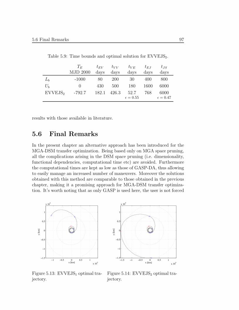
5.6 Final Remarks 97
Table 5.9: Time bounds and optimal solution for EVVEJS2.
TE tEV tV V tV E tEJ tJS
MJD 2000 days days days days days
Lb -1000 80 200 30 400 800
Ub 0 430 500 180 1600 6000
EVVEJS2 -792.7 182.1 426.3 52.7 768 6000! = 0.55 ! = 0.47
results with those available in literature.
5.6 Final Remarks
In the present chapter an alternative approach has been introduced for theMGA-DSM transfer optimization. Being based only on MGA space pruning,all the complications arising in the DSM space pruning (i.e. dimensionality,functional dependencies, computational time etc) are avoided. Furthermorethe computational times are kept as low as those of GASP-DA, thus allowingto easily manage an increased number of maneuvers. Moreover the solutionsobtained with this method are comparable to those obtained in the previouschapter, making it a promising approach for MGA-DSM transfer optimiza-tion. It’s worth noting that as only GASP is used here, the user is not forced
!1 !0.5 0 0.5 1
x 109
!1.5
!1
!0.5
0
0.5
1
x 109
x [km]
y [
km
]
Figure 5.13: EVVEJS1 optimal tra-jectory.
!1.5 !1 !0.5 0 0.5 1
x 109
!1.5
!1
!0.5
0
0.5
1
x 109
x [km]
y [
km
]
Figure 5.14: EVVEJS2 optimal tra-jectory.

98 Alternative Approach for MGA-DSM Transfers
to select the cuto! values for the DSM; in this way one of the pitfall of theGASP-DSM approach is avoided.

Chapter 6
Validated Optimization ofMGA Transfers
This chapter presents the attempt to solve the MGA transfer optimizationin a validated manner. The tool used to tackle this problem is the validatedglobal optimizer COSY-GO [15] which is based on the method of Remainder-enhanced Di!erential Algebra (RDA), also known as Taylor Model (TM)method. As this tool delivers the mathematically proven global optimum ofthe problem at hand, the potentials of its application to trajectory optimiza-tion problems are evident.
Some notes on RDA method are presented first based on the PhD thesisof Kyoko Makino [26]. We then give some hints on how these methods canbe used to develop a validated global optimizer, as done in COSY-GO. Theglobal optimization of Earth-Mars and a Earth-Venus-Mars transfers is thenaddressed and the achieved results critically discussed.
6.1 Di!erential Algebra and Interval Arith-metic
While DA methods can provide the derivatives of functional dependenciesand solutions of ODEs to high orders, in a rigorous sense they fail to pro-vide information about the range of the function. A simple example thatdramatically illustrates this phenomenon is the function shown in Figure 6.1
f(x) =
!
0 if x = 0exp(!1/x2) else.
(6.1)
The value of the function and all the derivatives at x = 0 are 0. Thusthe Taylor polynomial at the reference point x = 0 is just the constant

100 Validated Optimization of MGA Transfers
0. In particular, this also implies that the Taylor expansion of f convergeseverywhere, but it fails to agree with f(x) everywhere but at x = 0.
-0.2
0
0.2
0.4
0.6
0.8
1
1.2
-10 -8 -6 -4 -2 0 2 4 6 8 10
Figure 6.1: Function f(x) = exp(!1/x2) if x "= 0 ; 0 else, andits Taylor polynomial, which vanishes identically.
For the purpose of bounding functional dependencies, the methods ofinterval arithmetic provides a conceptual contrast. Both extended domainsof numbers as well as individual real numbers are represented via rigorousinclusions of floating point intervals. Arithmetic operations are introducedon intervals such that for any numbers in the intervals, a real arithmeticoperation on the two numbers always leads to a result that is contained inthe interval obtained from the corresponding arithmetic operation on theintervals. Table 6.1 lists some elementary properties of interval arithmetic.
By evaluating a function in interval arithmetic, it is thus possible tocarry rigorous bounds information through the operations, and in the endobtain rigorous bounds of the function. However, while reasonably fast inpractice, interval methods have some severe disadvantages, which limits theirapplicability for complicated functions. First, the width of resulting intervalsscales with the width of the original intervals; and second, artificial blow-upusually occurs in extended calculations. Another practical limitation arisesif scanning with small intervals is needed in the case of multiple dimensionsbecause of the fast increase of the computational expense.
To illustrate the blow-up phenomenon with a trivial example, we considerthe interval I = [a, b], which has the width b ! a. We compute the addition

6.2 Remainder-enhanced Di!erential AlgebraicOperations 101
Table 6.1: Elementary properties of interval arithmetic; I1 = [a1, b1], I2 =[a2, b2].
I1 + I2 = [a1 + a2, b1 + b2]
!I1 = [!b1,!a1]
I1 · I2 = [min(a1a2, a1b2, b1a2, b1b2), max(a1a2, a1b2, b1a2, b1b2)]
If 0 /" I1, 1/I1 = [1/b1, 1/a1]
of I to itself and its subtraction from itself:
I + I = [a, b] + [a, b] = [a + a, b + b] = [2a, 2b]
I ! I = [a, b] ! [a, b] = [a, b] + [!b,!a] = [a ! b, b ! a].
In both cases the resulting width is 2(b ! a), which is twice the originalwidth, although we know that regardless of what unknown quantity x ischaracterized by I, certainly x ! x should equal zero.
Polynomials under their conventional operations form a commutative al-gebra with unity. However, interval arithmetic does not have even a groupstructure for either addition or multiplication, since intervals with nonzerowidth have no inverses. Furthermore, instead of distributivity, we have thesub-distributivity,
I1 · (I2 + I3) # I1 · I2 + I1 · I3. (6.2)
The concepts of interval methods are discussed at length and in depth inseveral sources, as in [29].
6.2 Remainder-enhanced Di!erential AlgebraicOperations
RAD is a method that combines the advantage of rigor of the interval ap-proach, while largely avoiding the blow-up problem through the use of DAtechniques. The key idea is to describe the bulk of the functional dependence
102 Validated Optimization of MGA Transfers
through a Taylor polynomial, and bound the deviation of the original func-tion from the Taylor polynomial by an interval. In this endeavor, the Taylortheorem plays an important role.
Theorem (Taylor): Suppose that a function f : [!a,!b] ! Rv " R is(n+1) times continuously partially di!erentiable on [!a,!b]. Assume !x0 # [!a,!b].Then for each !x # [!a,!b], there is " # R with 0 < " < 1 such that
f(!x) =!n
!=01!!
"
(!x $ !x0) · !%#!
f(!x0) +
+ 1(n+1)!
"
(!x $ !x0) · !%#n+1
f (!x0 + (!x $ !x0)") ,
where the partial di!erential operator"
!h · !%#k
operates as
"
!h · !%#k
=$
0 ! i1, · · · , iv ! ki1 + · · · + iv = k
k!
i1! · · · iv!hi1
1 · · ·hivv
#k
#xi11 · · ·#xiv
v
.
Depending on the situation at hand, the remainder term also can be castinto a variety of well-known other forms.
Taylor’s theorem allows a quantitative estimate of the error that is to beexpected when approximating a function by its Taylor polynomial. Further-more, it even o!ers a way to obtain bounds for the error in practice, basedon bounding the (n + 1)st derivative, a method that has sometimes beenemployed in interval calculations.
Roughly speaking, Taylor’s theorem suggests that in many cases the errordecreases with the order as the width of the interval raised to the orderbeing considered, and its practical use is often connected to this observation.However, certain examples illustrate that this behavior does not have tooccur; one such example is (6.1) in the previous section.
For notational convenience, we introduce a parameter $ to describe thedetails of a given Taylor expansion, namely, the order of the Taylor polyno-mial n, and the reference point of expansion !x0. For the purpose to derivebounds for the remainder, it is also necessary to include the domain interval[!a,!b] on which the function is to be considered; altogether, we have
$ = (n, !x0, [!a,!b]). (6.3)
We now write an (n + 1) times continuously partially di!erentiable functionf : [!a,!b] ! Rv " R as a sum of its Taylor polynomial P",f of nth order anda remainder %",f as
f(!x) = P",f(!x $ !x0) + %",f(!x $ !x0),

6.2 Remainder-enhanced Di!erential AlgebraicOperations 103
where !!,f("x ! "x0) is continuous (even continuously di!erentiable) on thedomain interval and thus bounded. Let the interval I!,f be such that
""x # ["a,"b], !!,f("x ! "x0) # I!,f .
Then
""x # ["a,"b], f("x) # P!,f("x ! "x0) + I!,f . (6.4)
Because of the special form of the Taylor remainder term !!,f , in practicethe remainder usually decreases as |"x ! "x0|n+1. Hence, if |"x ! "x0| is chosento be small, the interval I!,f , which from now on we refer to as the intervalremainder bound, can become so small that even the e!ect of considerableblow-up is not detrimental. The set P!,f("x! "x0) + I!,f containing f consistsof the Taylor polynomial P!,f("x!"x0) and the interval remainder bounds I!,f .We say a pair (P!,f , I!,f ) of a Taylor polynomial P!,f("x!"x0) and an intervalremainder bounds I!,f is a Taylor model of f if and only if (6.4) is satisfied.In this case, we denote the Taylor model by
T!,f = (P!,f , I!,f).
We call n the order of the Taylor model, "x0 the reference point of the Taylormodel, ["a,"b] the domain interval of the Taylor model, and # the parameterof the Taylor model.
In the following, we develop tools that allow us to e"ciently calculateTaylor models for all functions representable on a computer. The key isto begin with the Taylor model for the identity function, which is trivial,and then successively build up Taylor models for the total function fromits pieces. This requires methods to determine Taylor models for sums andproducts from those of the summands or factors, as well as from intrinsicsapplied to functions with known Taylor model.
6.2.1 Addition and Multiplication
In this subsection, we discuss how a Taylor model of a sum or product oftwo functions can be obtained from the Taylor models of the two individualfunctions. This represents the first step toward the computation of Taylormodels for any function that can be represented on a computer.
Let the functions f, g : ["a,"b] $ Rv % R have Taylor models
T!,f = (P!,f , I!,f) and T!,g = (P!,g, I!,g),

104 Validated Optimization of MGA Transfers
which entails that
!!x " [!a,!b], f(!x) " P!,f (!x # !x0) + I!,f and
g(!x) " P!,g(!x # !x0) + I!,g.
Then it is straightforward to obtain a Taylor model for f + g; in fact, for any!x " [!a,!b],
f(!x) + g(!x) " (P!,f(!x # !x0) + I!,f ) + (P!,g(!x # !x0) + I!,g)
= (P!,f(!x # !x0) + P!,g(!x # !x0)) + (I!,f + I!,g),
so that a Taylor model T!,f+g for f + g can be obtained via
P!,f+g = P!,f + P!,g and I!,f+g = I!,f + I!,g. (6.5)
Thus we define
T!,f + T!,g = (P!,f + P!,g, I!,f + I!,g),
and we obtain that T!,f + T!,g = (P!,f+g, I!,f+g) is a Taylor model for f + g.Note that the above addition of Taylor models is both commutative andassociative.
The goal in defining a multiplication of Taylor models is to determine aTaylor model for f · g from the knowledge of the Taylor models T!,f and T!,g
for f and g. Observe that for any !x " [!a,!b],
f(!x) · g(!x) " (P!,f(!x # !x0) + I!,f) · (P!,g(!x # !x0) + I!,g)
$ P!,f(!x # !x0) · P!,g(!x # !x0)
+P!,f(!x # !x0) · I!,g + P!,g(!x # !x0) · I!,f + I!,f · I!,g.
Note that P!,f ·P!,g is a polynomial of (2n)th order. We split it into the partof up to nth order, which agrees with the Taylor polynomial P!,f ·g of ordern of f · g, and the extra polynomial Pe, so that we have
P!,f(!x # !x0) · P!,g(!x # !x0) = P!,f ·g(!x # !x0) + Pe(!x # !x0). (6.6)
A Taylor model for f · g can now be obtained by finding a bound intervalfor all the terms except P!,f ·g. For this purpose, let B(P ) be bounds of the
polynomial P : [!a,!b] % Rv & R, namely,
!!x " [!a,!b], P (!x) " B(P ).
Apparently the e!cient practical determination of B(P ) is not completelytrivial; depending on the order and number of variables, di"erent strategies

6.2 Remainder-enhanced Di!erential AlgebraicOperations 105
may be employed, ranging from analytical estimates to interval evaluations.However, thanks to the specific circumstances, the occurring contributionsare very small, and even moderate overestimation is not critical. Variousmethods for determining B(P ) will be discussed below.
Altogether, interval remainder bounds for f · g can be found via
I!,f ·g = B(Pe) + B(P!,f) · I!,g + B(P!,g) · I!,f + I!,f · I!,g. (6.7)
Thus we define T!,f · T!,g = (P!,f ·g, I!,f ·g), and obtain that T!,f · T!,g is aTaylor model for f · g. Note that commutativity of multiplication holds,T!,f · T!,g = T!,g · T!,f , while multiplication is not generally associative, andalso distributivity does not generally hold.
While the idea of Taylor models of constant functions is almost trivial,we mention it for the sake of completeness. For a constant function f(!x) ! t,the Taylor model of f is
T!,f ! T!,t = (P!,t, I!,t) = (t, [0, 0]).
Having introduced addition and multiplication as well as scalar multipli-cation, we can compute any polynomial of a Taylor model. Let Q(f) be apolynomial of a function f , that is, Q(f) = t0 + t1f + t2f 2 + · · · + tkfk. Inpractice it is useful to evaluate Q(f) via Horner’s scheme,
Q(f) = t0 + f ·!
t1 + f ·"
t2 + f · (· · · (tk!1 + f · tk) · · · )#
$
, (6.8)
in order to minimize operations. Furthermore, Horner’s scheme is often ofadvantage for interval related arithmetic because of the sub-distributivity(6.2) of interval arithmetic. Assume that we have already found the Taylormodel of the function f to be T!,f = (P!,f , I!,f). Then, using additions andmultiplications of Taylor models described above, we can compute a Taylormodel for the function Q(f) via
T!,Q(f) =%
P!,Q(f), I!,Q(f)
&
.
6.2.2 Intrinsic Functions
In the preceding subsection, we showed how Taylor models for sums andproducts of functions can be obtained from those of the individual functions.The computation led to the definition of addition and multiplication of Tay-lor models. Here we study the computation of Taylor models for intrinsicfunctions, including the reciprocal applied to a given function f from theTaylor model of f .

106 Validated Optimization of MGA Transfers
The key idea is to employ Taylor’s theorem of the function under consid-eration: However, in order to ensure that the resulting remainder term yieldsa small remainder interval and does not contribute anything to the Taylorpolynomial, several additional steps are necessary.
Let us begin the study with the exponential function. Assume thatwe have already found the Taylor model of the function f to be T!,f =(P!,f , I!,f). Write the constant part of the function f around !x0 as c!,f ,which agrees with the constant part of the Taylor polynomial P!,f , and writethe remaining part as f ; that is,
f(!x) = c!,f + f(!x).
A Taylor model of f is then T!,f = (P!,f , I!,f), where
P!,f(!x ! !x0) = P!,f(!x ! !x0) ! c!,f and I!,f = I!,f .
Now we can write
exp(f(!x)) = exp!
c!,f + f(!x)"
= exp(c!,f) · exp!
f(!x)"
= exp(c!,f ) ·#
1 + f(!x) +1
2!(f(!x))2 + · · ·+
1
k!(f(!x))k
+1
(k + 1)!(f(!x))k+1 exp
!
" · f(!x)"
$
,
where 0 < " < 1. Taking k " n, where n is the order of Taylor model, thepart
exp(c!,f) ·#
1 + f(!x) +1
2!(f(!x))2 + · · ·+
1
n!(f(!x))n
$
is a polynomial of f , of which we can obtain the Taylor model as outlined inthe preceding subsection. The remainder part of exp(f(!x)),
exp(c!,f) ·#
1
(n + 1)!(f(!x))n+1 + · · · +
1
(k + 1)!(f(!x))k+1 exp
!
" · f(!x)"
$
,
(6.9)
will be bounded by an interval. Since P!,f(!x ! !x0) does not have a constantpart, (P!,f(!x ! !x0))m starts from mth order. Thus, in the Taylor modelcomputation, the remainder part (6.9) has vanishing polynomial part. Theremainder bound interval for the Lagrange remainder term
exp(c!,f)1
(k + 1)!(f(!x))k+1 exp
!
" · f(!x)"

6.2 Remainder-enhanced Di!erential AlgebraicOperations 107
can be estimated because, for any !x ! [!a,!b], P!,f(!x " !x0) ! B(P!,f), and0 < " < 1, and so
(f(!x))k+1 exp!
" · f(!x)"
!!
B(P!,f) + I!,f
"k+1exp
!
[0, 1] · (B(P!,f) + I!,f )"
.
(6.10)
Since the exponential function is monotonically increasing, the estimation ofthe interval bounds of the part exp
!
[0, 1] · (B(P!,f ) + I!,f)"
is achieved byinserting the upper and lower bounds of the argument in the exponential.
Similar procedures can be used to obtain Taylor models for square root,multiplicative inverse of square root, sine, cosine, hyperbolic sine, hyperboliccosine, arcsine, arccosine, and arctanget. Altogether, it is now possible tocompute Taylor models along for any function that can be represented ina computer environment along with the mere evaluation of the function bysimple operator overloading, in much the same way as the mere computationof derivatives, Taylor polynomials, or interval bounds, along with the mereevaluation of the function.
6.2.3 Derivations and Antiderivations
In the spirit of the idea of embedding the elementary operations of addition,multiplication, and di!erentiation and their inverses that are defined on theclass of C! functions onto the structure of Taylor Models, we now come tothe mapping of the derivation operation # as well as its inverse #"1. Similarto the case of the DA, and following one of the main thrusts of the historyof di!erential algebra, we will use these for the solution of the initial valueproblem
d
dt!r(t) = !F (!r(t), t),
where !F is continuous and bounded. We are interested in both the case of aspecific initial condition !r0, as well as the case in which the initial condition!r0 is a variable, in which case our interest is in the flow of the di!erentialequation
!r(t) = M(!r0, t).
As in the case of the conventional DA method, in order to prevent loss oforder in the di!erentiation process, the derivation # can be evaluated onlyin the context of a Lie derivative Lg = g · #, where g(!x0) = 0. However,in the case of Taylor models, an additional complication is connected to the

108 Validated Optimization of MGA Transfers
fact that from the Taylor model alone, it is impossible to determine boundsfor the derivative, since nothing is known about the rate of change of thefunction (f ! P!,f) within the remainder bounds If . The situation can beremedied by a further extension of the Taylor model concept to contain notonly bounds for the remainder, but also a low-parameter bounding sequencefor all the higher derivatives that can occur. In contrast to the derivation !,Taylor models of its inverse !!1 are readily available.
Given an n-th order Taylor model (Pn,f , In,f) of a function f : ["a,"b] "Rv # R around the reference point "x0, we can determine a Taylor model forthe indefinite integral !!1
i f =!
f dxi with respect to the variable xi. TheTaylor polynomial part is obviously just given by
! xi
0 Pn!1,f("x)dxi. Since thepart of the Taylor polynomial Pn,f that is of precise order n is Pn,f !Pn!1,f ,remainder bounds can be obtained as (B(Pn,f !Pn!1,f)+ In,f) ·B(xi), whereB(xi) is obtained from the range of definition of xi as bi !ai. We thus definethe operator !!1
i on the space of Taylor models as
!!1i (Pn,f , In,f) = (Pn,"!1f , In,"!1f)
=
"# xi
0
Pn!1,f("x)dxi , (B(Pn,f ! Pn!1,f) + In,f) · B(xi)
$
. (6.11)
With this definition, bounds for a definite integral over variable xi from xil toxiu both in [ai, bi], the domain of validity of the Taylor model of a function,can be obtained as
# xij
xil
f ("x)dxi $ (Pn,"!1f("x|xi=xiu!xi0)!Pn,"!1f ("x|xi=xil!xi0
), In,"!1f). (6.12)
6.3 Examples
RDA have many applications, including global optimization, quadrature, andsolution of di!erential equations. We begin our discussion with the deter-mination of sharp bounds for a simple example function using RDA. Thesharpness of the resulting bounds will be compared with the results that canbe obtained in other ways. Secondly, we show schematically how the methodcompares with the interval method to obtain bound enclosures of functionsin one and two dimensional cases.
6.3.1 A Simple Function
The function under consideration is
f(x) =1
x+ x. (6.13)

6.3 Examples 109
For an actual computation, we set the parameter ! of (6.3) to ! = (n, x0, [a, b])= (3, 2, [1.9, 2.1]).
As in the case of DA, the evaluation begins with the representation of theidentity function, expressed in terms of a Taylor polynomial expanded at thereference point. This identity function i has the form
i(x) = x = x0 + (x ! x0) = 2 + (x ! 2).
Since this representation is exact, the remainder bound interval is [0, 0].Hence, a Taylor model of the identity function i is
T!,i = (x0 + (x ! x0), [0, 0]) = (2 + (x ! 2), [0, 0]).
The constant part of i around x0 = 2 is c!,i = x0 = 2, and the nonconstantpart of i is i(x) = x ! x0 = x ! 2. The Taylor model of i is
T!,i = ((x ! x0), [0, 0]) = ((x ! 2), [0, 0]) .
The computation of the inverse requires the knowledge of bounds of P!,i,which here is readily obtained: B(P!,i) = B(x ! x0) = [a ! x0, b ! x0] =[!0.1, 0.1]. We have furthermore B(P!,i) + I!,i = [!0.1, 0.1] + [0, 0] =[!0.1, 0.1]. Using (6.6) and (6.7), we have for the Taylor model of (i)2
T!,(i)2 =!
(x ! 2)2, [0, 0]"
.
The Taylor model of (i)3 is computed similarly: T!,(i)3 = ((x ! 2)3, [0, 0]). Ascan be seen, so far all remainder intervals are of zero size. The first nonzeroremainder interval comes from the evaluation of the Taylor remainder term,which is
(i(x))4
c5!,i
1
(1 + " · i(x)/c!,i)5 "
(B(P!,i) + I!,i)4
x50 ·
!
1 + [0, 1] · (B(P!,i) + I!,i)/x0
"5(6.14)
#[0, 0.0001]
25 · ([0.95, 1.05])5# [0, 4.038 $ 10!6].
As expected, this remainder term is “small of order four”. The Taylor modelof 1/i is
T!, 1i
=
#
1
2!
1
22(x ! 2) +
1
23(x ! 2)2 !
1
24(x ! 2)3, [0, 4.038 $ 10!6]
$
,

110 Validated Optimization of MGA Transfers
and the remainder interval is indeed still very sharp. Using (6.5), we obtainas the final Taylor model of 1/i + i
T!, 1i+i = T!, 1
i+ T!,i =
!
P!, 1i+i, I!, 1
i+i
"
(6.15)
=
##
2 +1
2
$
+
#
1 !1
22
$
(x ! 2) + (6.16)
1
23(x ! 2)2 !
1
24(x ! 2)3, [0, 4.038 " 10!6]
$
=%
2.5 + 0.75(x ! 2) + 0.125(x! 2)2 ! 0.0625(x! 2)3, [0, 4.038 " 10!6]&
.
Since the polynomial P!, 1i+i is monotonically increasing in the domain
[a, b] = [1.9, 2.1], the bound interval of the polynomial is
B!
P!, 1i+i
"
='
P!, 1i+i(!0.1), P!, 1
i+i(0.1)
(
= [2.42631, 2.57618].
The width of the bound interval of the Taylor polynomial is 0.14987, andthe width of the remainder bound interval is 4.038" 10!6 in the third-orderTaylor model evaluation; thus the remainder part is just a minor addition.The size of the remainder bounds depends strongly on the order and decreasesquickly with order.
The Taylor model computation is assessed by noting the bound intervalB of the original function (6.13), which is
B
#
1
x+ x
$
=
)
1
a+ a,
1
b+ b
*
= [2.42631, 2.57619].
It is illuminating to compare the sharpness of the bounding of the functionwith the sharpness that can be obtained from conventional interval methods.Evaluating the function with just one interval yields
1
[a, b]+ [a, b] =
1
[1.9, 2.1]+ [1.9, 2.1] # [2.37619, 2.62631].
The width of the bound interval obtained by interval arithmetic is 0.25012,and so this simple example already shows a noticeable blow-up. By dividingthe domain interval into many subintervals, the blow-up can be suppressedsubstantially. However, to achieve the sharpness of the third-order Taylormodel, the domain has to be split into about 24, 000 subintervals.
Practically more important are optimization problems in several vari-ables, and in this case, the situation becomes more dramatic. We wish firstto illustrate the computational e!ort necessary for an accurate calculation of

6.3 Examples 111
Table 6.2: The total number of FP operations required to bound a simplefunction like f(!x) =
!
j(1/xj + xj).
One Dimensional Six DimensionalInterval ! 10 ! 10104 divided intervals ! 105 ! 1025
3rd order Taylor model ! 10 ! 104
the result by estimating the required number of floating-point operations. Weuse a simple example function of six variables such as f(!x) =
!
j(1/xj+xj) toget a rough idea of the computational expense in the case of functions of manyvariables. In the one-dimensional case, one interval calculation 1/[a, b]+[a, b]requires two additions and two divisions. To compare with the third-orderTaylor model computation, we divide the domain into 104 subintervals, onwhich additions and divisions total !105 floating-point operations. Thus,in the multidimensional case with six independent variables, the number offloating-point operations explodes to (104)6 " (!10) = !1025. Again, so-phisticated interval optimization methods will be more favorable than thesenumbers suggest, but typically there is still a very noticeable growth of com-plexity.
To estimate the performance of the Taylor model approach, we note thatthe one-dimensional Taylor model in the third-order computation involves atotal of about 35 additions, multiplications, and divisions. As we use morevariables, however, the total number of terms in the polynomial grows onlymodestly. For example, order three in six variables requires only a total of 84terms. Thus in total, the number of floating-point operations of the third-order Taylor model is !104. A summary of the number of floating-pointoperations is given in Table 6.2.
6.3.2 Bound Enclosures of Functions
In this subsection, we use some simple functions in one dimension and twodimensions to show schematically how the RDA method bounds functions incomparison with the interval method. The first function is a one dimensionalfunction
f(x) = x(x # 1.1)(x + 2)(x + 2.2)(x + 2.5)(x + 3) · sin(1.7x + 0.5).
Figure 6.2 shows the function and its bound enclosures in the domain [#0.5, 1.0].The interval method is applied to bound the function using smaller domain

112 Validated Optimization of MGA Transfers
intervals divided into 25 subintervals and 50 subintervals. The method ofTaylor models computes the polynomial part of the function and the re-mainder bound interval. The pictures show the bands of the enclosures ofthe function around its polynomial parts by the remainder bounds using 8thorder Taylor models.
Figure 6.2: One dimensional function and its bound enclosures. From top tobottom right: the function, the bounds by the interval method with the 25and 50 divided domain intervals, the bound by the 8th order Taylor models.
A similar schematical comparison between the interval method and themethod of Taylor models is made for a two dimensional function. We workedon a function
f(x, y) = sin(1.7x + 0.5) · (y + 2) · sin(1.5y)
in the domain [!1, 1] " [!1, 1]. Figure 6.3 shows the function enclosures bythe interval method with the smaller domain intervals divided into 10 " 10,20"20, 40"40 and 80"80. Figure 6.4 shows the function enclosures aroundits polynomial parts by the remainder bounds using 7th, 8th, 9th and 10thorder Taylor models. Even in this modest case of only two dimensions,

6.4 Notes on COSY-GO 113
the Taylor model approach requires much less e!ort to provide a similarlevel of sharpness; the 1600 subintervals used to include the function are incontrast to only 66 expansion coe"cients, plus one remainder bound interval.As dimension is increased, the number of subintervals necessary to providean accurate modeling increases dramatically, while the number of Taylorcoe"cients grows much more slowly.
Figure 6.3: Bound enclosures of a two dimensional function by the intervalmethod. From top to bottom right: The domain is divided to 10!10, 20!20,40 ! 40 and 80 ! 80 subintervals.
6.4 Notes on COSY-GO
COSY-GO [15] is a classical branch-and-bound optimization algorithm whichtakes advantages of the bounding performances assured by TM methods.Suppose we want to find the global minimum of a su"ciently regular scalar

114 Validated Optimization of MGA Transfers
function f on a given domain A ! "m. The algorithm starts with an initialguess for the global optimum, the cuto! value, and it proceeds by analyzingat each step a subdomain for possible elimination. At each step the followingtasks are performed.
a) A lower bound l of the function is obtained using various boundingschemes in a hierarchical manner. If the lower bound is above thecuto! value, the box is eliminated; if not, the box is bisected. As afirst test the polynomial part of the objective function is evaluatedin interval arithmetic. When it fails to eliminate the box, a lineardominated bounder (LDB) is used and possible domain reduction isexecuted. If it also fails to eliminate the box, and if the quadratic partof the polynomial representation of the objective function P is positivedefinite, a quadratic fast bounding is performed.
b) The cuto! value is updated using various schemes. The linear andquadratic parts of P are utilized to obtain a potential cuto! update.In particular, if the quadratic part of the polynomial is positive definite,the minimizer of the quadratic polynomial is tested. If the quadraticpart is not positive definite, the minimizer of the quadratic part in thedirection of the negative gradient is tested.
The algorithm continues to split and examine the domain until the minimumdimension allowed is reached. The result of the otpimization is the validatedenclosure of the minimum of the problem.
6.5 Validated Solution of Implicit Equations
As seen in previous chapter the evaluation of the overall "v of a MGA trans-fer requires the solution of implicit equations. In the first chapter we haveshown how the Taylor expansion of the solution manifold can be obtained bymeans of DA. In order to address the validated optimization of MGA transferssomething additional is required. The computation involved in the objectivefunction evaluation must be performed in validated manner indeed, includingthe solution of implicit equation. In the following the validated solution of ascalar implicit equation is detailed, the extension to the m dimensional caseis omitted.
Let P (x) + I be an n-th order Taylor model of the (n +1) times di!eren-tiable function f over the domain D = [#1; 1] so that
f(x) $ P (x) + I for all x $ D (6.17)

6.5 Validated Solution of Implicit Equations 115
Let R be an enclosure of the range of P (x) + I over D. Assume P hasnonvanishing derivative everywhere in D; without loss of generality P ismonotonically increasing, and P !(x) > d > 0 on D.
Problem: Find a Taylor model c(y) + J on R such that any solution x ! Dof the problem f(x) = y lies in
c(y) + J. (6.18)
Without loss of generality, we assume P (0) = 0. First, determine the poly-nomial c(y) = c1y + c2y2 + . . . by DA inversion of P in the well known way,so that we have
P (c(y)) =n y. (6.19)
Indeed, c(y) is the n-th order Taylor polynomial of the inverse of f at thepoint 0 = P (0). It has the property that for any given y it gives an ap-proximate value x = c(y) that satisfies P (x) " y, and thus also f(x) " y,depending on how well the inverse is representable by its Taylor expansionover the domain R. However, it is not the true inverse: if we evaluate P (c(y))in n-th order Taylor model arithmetic, we obtain P (c(y)) ! y + J , where Jis due to the terms of orders exceeding n in P (c(y)); and thus scales with atleast order (n + 1).
Next we want to find a rigorous remainder J for c(y) so that all solutionsof f(x) = y lie in c(y)+J . We do this by studying the consequences of smallcorrections x to c(y). We observe that, according to the mean value theorem,
f(c(y) + !x) # y ! P (c(y) + !x) # y + I= P (c(y)) + !x · P !(!) # y + I$ y + J + !x · P !(!) # y + I= !x · P !(!) + I + J
(6.20)
for some suitable ! that lies between c(y) and c(y) + !x. However, since on[#1; 1], P ! is bounded below by d, we observe that in [#1; 1], but outside ofthe interval
J = #I + J
d(6.21)
the set !x · P !(!) + I + J will never contain zero, and thus no solution off(c(y) + !x) # y exist there. So we obtain:
Theorem. Any solution x ! D = [#1; 1] of f(x) = y lies in the Taylormodel c(y) + J .
Let us make some remarks.

116 Validated Optimization of MGA Transfers
1) No information on the derivative f ! is needed, which is helpful in prac-tice.
2) Indeed, if f is not monotonic, it is conceivable that c(y) + J containsmultiple solutions of f(x) = y
3) For any y ! [P ("1) + u(I); P (+1) + l(I)], at least one solution existsdue to the intermediate value theorem.
4) For any y /! [P ("1) + l(I); P (+1) + u(I)], no solution exists
As an important consequence, we obtain the following:
Corollary. If f is invertible over D, c(y) + J is a Taylor model of order(n + 1) of its right inverse.
6.6 Test Cases
Two test cases are addressed, the first one is a simple planet-to-planet transferwhereas the second exploits a gravity assist. As it will be shown the additionof a single gravity assist significantly complicates the optimization problem.
6.6.1 EM
The first test case is an Earth-Mars transfer. This problem is representativeof any planet-to-planet transfer as it involves only two ephemerides evalu-ations and one Lambert’s problem solution. The transfer is formulated indeparture epoch and time of flight in order to deal with a rectangular searchdomain, thus easing the branch-and-bound algorithm implemented in COSY-GO. As no GA is considered, we deal with an unconstrained optimizationproblem, and this is particularly beneficial as COSY-GO does not explic-itly handle constraints. The search space and the enclosure of the optimalsolution is shown in Table 6.3.
The enclosure of the optimal !v is [5.6673264, 5.6673272] km/s whichincludes the optimal solution of 5.6673270 km/s found with GASP and in-dicated in Figure 6.5 with the red star. The price to pay for obtaining thevalidated optimum solution is the computational time: the optimization pro-cess takes 4954.39 s on a Pentium IV 3.06 GHz laptop platform. The mainreason of this result is the presence of discontinuity lines of the objectivefunction within the search domain. Whenever a discontinuity is found in abox, the validated evaluation of the objective function is an algebraic failure.In these cases the optimizer is forced to split the domain until the minimum

6.6 Test Cases 117
Table 6.3: Time bounds and enclosure of the optimal solution for EM transfer
TE tEM
MJD 2000 days
Lb 1000 100Ub 6000 600EM [3573.176, 3573.212] [324.034, 324.088]
box size is reached. This situation is clear by looking at Figure 6.6 whichshows that most of the iterations do not bring any improvement in the cuto!value.
At the end of the optimization the remaining domain includes both thebox containing the optimal solution and the boxes which contains discontinu-ities. For this reason the result can not be considered the validated enclosureof the solution, but rather the global optimum from an engineering pointof view. Indeed it is improbable to find a better enclosure of the solutionamong boxes with algebraic failures as a very small minimum box size is set.Furthermore it’s worth noting that the objective function discontinuities arenot physical but the result of the problem formulation (Lambert’s problemsolution). In order to achieve a mathematical proven optimal solution a dif-ferent formulation of the problem, which avoids the solution of the Lambert’sproblem, should be adopted.
6.6.2 EVM
The second test case considers a transfer to Mars and includes a Venus GA.The simple addition of a GA makes the problem tougher as the constrainton the minimum pericenter altitude must be considered. As COSY-GO is anunconstrained optimizer there are two possible ways to deal with constraints:penalty functions and space pruning. The first one consists in augmentingthe objective function with a term representative of the constraint violation.The second one assigns an arbitrary high value to the objective functionwhenever a box entirely violates the constraint. The result presented hereuses the second technique. The main advantage is that no weighting factormust be chosen; on the other hand there’s the possibility that the optimalsolution found violates the constraint. This problem is unlikely to happen ifthe minimum box dimension allowed is very small.
Table 6.4 shows the problem definition as well as the enclosure of theoptimal solution. It’s worth noting that, unless the results are presented

118 Validated Optimization of MGA Transfers
Table 6.4: Time bounds and enclosure of the optimal solution for EVMtransfer
TE tEV tV M
MJD 2000 days days
Lb 5000 140 200Ub 6000 240 400EVM [5611.475, 5611.512] [157.592, 157.623] [255.564, 255.620]
in term of departure epoch and time-of-flights, the optimization problem isformulated in absolute times in order to reduce the functional dependencies.The enclosure of the optimal minimum is !v ! [8.5220251, 8.5231393] km/swhich includes the optimal value of 8.5226 obtained with GASP.
The increased problem dimension has a dramatic impact on the compu-tational time; the optimization process takes about three weeks on the sameplatform used for the previous test indeed. The boxes that includes a discon-tinuity must be split until all the three sizes are under the minimum valueallowed, thus causing a blow-up in the computational time even when a smallsearch domain is analyzed.
6.7 Final Remarks
The TM-based validated optimizer is a potential tool for finding the globaloptimum of any MGA transfer. On the other hand, several issues must beaddressed to make its use viable for complex MGA transfers. A method formanaging the discontinuities is necessary; to this aim an ad hoc problemformulation could be a viable option. Furthermore a more e"cient and safemethod to handle the constraints is mandatory. A possible solution is rep-resented by the explicit computation of the constraint manifold. Finally thereduction of the computational time could be achieved by running COSY-GO in parallel on several machines. In any case the large computational timeenlightened in the previous section is the price to pay for gaining a validatedenclosure of the optimal solution.

6.7 Final Remarks 119
Figure 6.4: Bound enclosures of a two dimensional function by the RDAmethod. From top to bottom right: Computations in 7th, 8th, 9th and 10thorder Taylor models.

120 Validated Optimization of MGA Transfers
!v
[km
/s]
Figure 6.5: Objective function val-ues and optimal solution found.
0 0.5 1 1.5 2 2.5
x 105
5.5
6
6.5
7
7.5
8
8.5
9
9.5
10
10.5
Iteration #
Cuto
ff v
alu
e [
km
/s]
Figure 6.6: !v cuto" history.

Chapter 7
Conclusions and Final Remarks
This chapter is devoted to trace the work described throughout the report,and to identify key points for possible future developments. The final remarkspertaining the pruning and optimization of MGA transfers involving DSMare first presented, whereas special comments are dedicated to the validatedglobal optimization of MGA transfers.
A version of the classical pruning algorithm GASP, based on the useof di!erential algebraic techniques, has been implemented and described inchapter 3. Significant work was aimed at addressing the discontinuity anddependency problems. The major solution to the discontinuity problem wasthe use of a planar planetary model for the Solar System. Based on theobservation that the discontinuity corresponding to the transition from theshort–way to the long–way solution of the Lambert’s problem disappears,the planar model is used to perform the pruning process. Furthermore, con-sidering the low inclinations of all planetary orbits, the overall "V associ-ated to the planar model has been conjectured to be usually lower than thecorresponding "V in the actual three–dimensional model. Consequently,no information and solutions are lost by performing the pruning processin the planar model, and then optimizing the transfer in the actual three–dimensional model. The dependency problem was solved by replacing theclassical relative times formulation for MGA transfer optimization problems,with the e!ective absolute times formulation, based on the use of the epochsat each planet as design variables. As demonstrated by the test phase, theresulting algorithm GASP–DA turns out to e!ectively prune and optimizeMGA transfers without DSM.
Then, GASP–DA has been extended to include DSM. Chapter 3 showedthat a dependency problem still occur, which is evidently similar to the sameproblem in classical MGA transfers. This led to the necessity of modeling

122 Conclusions and Final Remarks
the whole transfer as a sequence of Lambert’s arcs, which corresponds toadopt a formulation, which has been again referred to as absolute variablesformulation. Several successful test cases have been carried out to assess theperformances of the resulting algorithm.
The use of the resulting GASP–DSM–DA algorithm is not free of sig-nificant drawbacks. First of all, a problem related to the allocated memorycan be identified. In particular, as reported in chapter 2, a DA number is avector of (n + v)!/(n! v!) coe!cients, where n is the order of the correspond-ing expansion and v is the number of variables. Consequently, the vectorsize quickly increases with n and v (see [14] for further details). It is worthhighlighting that many coe!cients are usually equal to zero in practical com-putations. However, the tool COSY INFINITY, that implements di"erentialalgebra and has been used within this work, does not allow to dynamicallyallocate memory. Consequently, a great amount of memory must be allo-cated anyway at the beginning of the computation, which often increasesprohibitively in practical computations.
A further drawback is associated again to the dependency problem. Specif-ically for MGA transfers involving DSM, three variables must be added to theset of design variables for each additional DSM. Given the structure of theMGA–DSM problem, and the periodicities associated to most of the entailedvariables, the multimodality of the optimization problem increases with thenumber of DSM introduced, and a growing number of local minima tendsto characterize the optimization landscape. In such a complicated frame-work, Taylor expansions tend to lose their accuracy, and smaller box sizesare required to reach reasonable pruning performances. Alternative approx-imation techniques might worth further investigation in this scenery, as theuse of Fourier series to replace Taylor series when periodicities occur.
The pruning process of MGA transfers, including or not DSM, is anywayaimed at easing the subsequent necessary optimization phase. Thanks tothe imposed constraints, large parts of the search space are intended to bepruned away. In this way, the e"ectiveness of the optimization algorithmsat identifying the actual global optimum of the original problem is finallyenhanced. Given the steep increase of computational burden, associated tothe pruning of MGA transfers involving DSM, alternative strategies havebeen sough to solve the ultimate optimization problem, which have beendescribed in chapter 5. Specifically, considering the high e!ciency of GASPand GASP–DA when pruning MGA transfers without DSM, an alternativestrategy has been developed. Given the sequence of planets involved in aMGA transfer:
1. GASP–DA is used to identify a set of good solutions for the MGA

Conclusions and Final Remarks 123
transfer, without considering the introduction of DSM;
2. based on the concept of Pareto–optimality, solutions are selected fromthe previous set;
3. DSM are introduced based on suitable heuristics;
4. the corresponding solutions are used as first guesses for a subsequentoptimization process.
Despite the algorithm does not rely directly on search space pruning of MGAtransfers involving DSM, it proves some important advantages when com-pared to GASP–DSM–DA. First of all, the optimization process is carriedout in less computational time, and larger search spaces can be processedwith a!ordable computational burden. Moreover, the optimal solutions arecomparable in many transfers of practical interest, as shown by Table 7.1.
Table 7.1: Comparison of the three developed methods in terms of optimal"v.
"v [m/s]GASP–DA GASP–DA DSM DSM Altern.
EVM 8.523 8.167 8.081
EMJ 13.42 12.481 12.394
EMMJ 12.864 10.843 10.968
EVEEJ 10.09 8.670 8.687
EVEME 12.443 10.931 10.874
EVVEJS 8.619 8.299 8.588
Clearly, all the implemented pruning and optimization algorithms are notfree of further possible improvements. First of all, pertaining GASP–DA, akey-point for significant enhancements is including the automatic selectionof the optimal planets sequence within the optimization process. This wouldlead to a mixed continuous–combinatorial optimization problem, whose so-lution can be extremely di#cult, especially if a high number of planets forGA maneuvers is considered. Moreover, concerning both GASP–DSM–DAand the alternative strategy developed in chapter 5, the possibility of insert-ing more than one DSM per arc should be addressed. This advance serves

124 Conclusions and Final Remarks
the purpose using DSM to approximate low–thrust transfers at the begin-ning of the design phase, as widely suggested in the space–trajectory designcommunity. Within the framework of low–thrust arcs modeling during thepreliminary phases of space–trajectory design, a further important step willbe the introduction of exponential sinusoid in GASP–DA. Based on the workof Izzo [22], the Lagrange equation for the time of flight is substituted byan alternative implicit equation, which needs to be solved within di!erentialalgebra, using techniques similar to the one presented in chapter 2.
Separate comments are instead dedicated to the validated global opti-mization of MGA transfers investigated in chapter 6. It is worth gainingmore valuable insights on the main drawbacks encountered, and proposingpossible promising solutions. As highlighted in chapter 6, the main di"cultyis identified to be related to the management of constraints in COSY–GO.Referring to Figure 7.1, suppose the function obj must be minimized. A box[X] is being processed and part of the box turns out to be unfeasible underthe imposed constraints. The current version of COSY–GO does not handleconstraints automatically, especially if boxes lying on the constraint manifoldare being analyzed. Consequently, the box in Figure 7.1 would be consideredas entirely feasible if no expedients are used. Suppose now a Taylor modelevaluation of the objective function over [X] is performed, which leads tothe range reported in Figure 7.2. The algorithm now tries to update thecuto! value for the optimization process using the estimation from aboveof the minimum of the objective function over [X]. The exact estimationfrom above of the minimum within the box is reported as obj
!
min in Figure7.2. However, if the whole box [X] was considered as entirely feasible, theestimation actually used by COSY–GO would be objmin, which clearly un-derestimate the actual feasible minimum ¯obj
!
min. The main consequence isthat, if objmin is used to update the cuto! value for the optimization process,actual solutions might be pruned away. Intensive investigations must be de-voted to overcome this problem. Besides the possibility of adding constraintsto the objective function as penalty terms, which might turn out to modifythe landscape of the original objective function within the feasible region ofthe search space, an alternative solution can be outlined. Ad–hoc techniquesexist to compute validated enclosures of the constraint manifolds, which arebased on the use of Taylor models. In this way, given a box to be processed,the validated enclosure is used to rigorously identify the feasible regions ofthe box. The objective function is the evaluated over these regions only, andthe resulting estimated minimum can be correctly used to update the cuto!value for the optimization process.
A further drawback of the use of COSY–GO for MGA transfers is thesteep increase of the computational time with the number of design vari-

Conclusions and Final Remarks 125
Figure 7.1: Constraint managementin COSY–GO.
Figure 7.2: Underestimation of theactual minimum.
ables, which does not exploit the problem structure in the default setting, asperformed in GASP. Suitable adjustments on the current version of COSYcan be considered as viable solutions for future applications. However, it isworth observing that the versatility of COSY–GO has an important bene-fit: COSY–GO algorithm is fully parallelizable. This means that the sameoptimization process can be distributed on an high number of processors tosignificantly reduce the computational time.

126 Conclusions and Final Remarks

Bibliography
[1] Ascher, U., and Petzold, L., Computer Methods for Ordinary Di!eren-tial Equations and Di!erential-Algebraic Equations, SIAM, 1998.
[2] Battin, R.H., An Introduction to the Mathematics and Methods of As-trodynamics, Revised Edition, AIAA Education Series, 1999.
[3] Berz, M., “The new method of TPSA algebra for the description ofbeam dynamics to high orders”, Technical Report AT-6:ATN-86-16,Los Alamos National Laboratory, 1986.
[4] Berz, M., “The method of power series tracking for the mathemati-cal description of beam dynamics”, Nuclear Instruments and MethodsA258, 431, 1987.
[5] Berz, M., “Di!erential algebraic description of beam dynamics to veryhigh orders”, Technical Report SSC-152, SSC Central Design Group,Berkeley, CA, 1988.
[6] Berz, M., Fawley, B., and Hahn, K., “High order calculation of the mul-tipole content of three dimensional electrostatic geometries”, NuclearInstruments and Methods A307, 1, 1991.
[7] Berz, M., “High-Order Computation and Normal Form Analysis ofRepetitive Systems,” Physics of Particle Accelerators, Volume AIP249, pp. 456, 1991.
[8] Berz, M., “COSY INFINITY Version 6”, In M. Berz, S. Martin, andK. Ziegler (Eds.), Proc. Nonlinear E!ects in Accelerators, page 125,IOP Publishing, 1992.
[9] Berz, M., “Automatic di!erentiation as nonarchimedean analysis”, InComputer Arithmetic and Enclosure Methods, Amsterdam, page 439,Elsevier Science Publishers, 1992.

128 Bibliography
[10] Berz, M., “New features in COSY INFINITY”, In Third Computa-tional Accelerator Physics Conference, page 267, AIP Conference Pro-ceedings 297, 1993.
[11] Berz, M., Ho!statter, G., Wan, W., Shamseddine, K., and Makino,K., “COSY INFINITY and ist application to nonlinear dynamics”, InComputational Di!erentiation: Techniques, Applications, and Tools,M. Berz, C. Bischof, G Corliss, and A. Griewank (Eds.), SIAM, 1996.
[12] Berz, M., “COSY INFINITY version 8 reference manual”, TechnicalReport MSUCL-1088, National Superconducting Cyclotron Labora-tory, Michigan State University, East Lansing, MI 48824, 1997.
[13] Berz, M., “Di!erential Algebraic Techniques”, Entry in “Handbook ofAccelerator Physics and Engineering”, M. Tigner and A. Chao (Eds.),World Scientific, 1999.
[14] Berz, M., Modern Map Methods in Particle Beam Physics, AcademicPress, 1999.
[15] Berz, M., Makino, K., and Kim, Y., “Long-term stability of the teva-tron by verified global optimisation”, Nuclear Instruments and Meth-ods, A558, pp. 1-10, 2005.
[16] Di Lizia, P., and Radice, G., “Advanced Global Optimisa-tion for Mission Analysis and Design”, Final Report, Ariadnaid: 03/4101, Contract No. 18139/04/NL/MV, 2004. (Availableat: http://www.esa.int/gsp/ACT/doc/ACTRPT-03-4101-ARIADNA-GlobalOptimisationGlasgow.pdf)
[17] Di Lizia, P., Radice, G., and Vasile, M., “On the solution of interplan-etary trajectory design problems by global optimisation methods”, In-ternational Workshop on Global Optimisation, Almerıa, Spain, 18-22September, 2005.
[18] Gobetz, F., “Optimal transfer between hyperbolic asymptotes”, AIAAJournal, 1, 1963.
[19] Griepentrog, E., and Marz, R., Di!erential-Algebraic Equations andTheir Numerical Treatment, Teubner, 1986.
[20] He, J., Watson, L., Ramakrishnan, N., Sha!er, C. A., Verstak, A.,Jiang, J., Bae, K., and Tranter, W., “Dynamic data structures for adirect search algorithm”, Technical Report TR-01-09, Computer Sci-ence, Virginia Tech, 2001.

Bibliography 129
[21] Izzo, D., Becerra, V., Myatt, D., Nasuto S., and Bishop, J., “Searchspace pruning and global optimisation of multiple gravity assist space-craft trajectories”, Journal of Global Optimisation, 38, pp. 283–296,2006.
[22] Izzo D., “Lamberts problem for exponential sinusoids”, Journal ofGuidance, Dynamics, and Control, 29, pp. 1242–1245, 2006.
[23] Izzo, D., “Advances in Global Optimisation for Space Trajectory De-sign”, 25th International Symposium on Space Technology and Science,2006.
[24] Jones, D., “A taxonomy of global optimisation methods based on re-sponse surfaces”, Journal of Global Optimisation, 21, pp. 345–383,2001.
[25] Kennedy, J., and Eberhart, R., “Particle swarm optimisation”, Proc.IEEE Int. Conf. on Neural Networks, pp. 1942–1948, 1995.
[26] Makino, K., “Rigorous Analysis of Nonlinear Motion in Particle Ac-celerators”, Ph.D. Thesis, Michigan State University, East Lansing,Michigan, USA, 1998.
[27] Michelotti, L., “MXYZTPLK: A practical, user friendly c++ imple-mentation of di!erential algebra”, Technical Report, Fermilab, 1990.
[28] Myatt, D., Becera, V., Nasuto, S., and Bishop, J., “AdvancedGlobal Optimisation for Mission Analysis and Design”, FinalReport, Ariadna id: 03/4101, Contract No. 18138/04/NL/MV,2004. (Available: http://www.esa.int/gsp/ACT/doc/ACT-RPT-03-4101-ARIADNA-GlobalOptimisationReading.pdf)
[29] Moore, R.E., Interval Analysis. Prentice Hall, Englewood Cli!s, NJ,1966.
[30] Van Zeijts, J., and Neri, F., “The arbitrary order design code TLIE1.0”, In M. Berz, S. Martin, and K. Ziegler (Eds.), Proceedings Work-shop on Nonlinear E!ects in Accelerators, IOP Publishing, 1993.
[31] Vasile, M., and De Pascale, P. “Preliminary Design of Multiple Gravity-Assist Trajectories”, Journal of Spacecraft and Rockets, Vol. 43, N. 4,pp. 794–805, 2006.

130 Bibliography
[32] Vinko, T., Izzo, D., and Bombardelli, C. “Benchmarking di!erentglobal optimisation techniques for preliminary space trajectory design”58th International Astronautical Congress, Hyderabad, India, 2007.
[33] Yan, Y., “ZLIB and related programs for beam dynamics studies”, InThird Computational Accelerator Physics Conference, pp. 279, AIPConference Proceedings, 297, 1993.