global positioning system (gps) radio occultation … of radio occultation products at noaa/jcsda !!...
TRANSCRIPT

Global Positioning System (GPS)
Radio Occultation (RO)
Data Assimilation
Lidia Cucurull
NOAA & JCSDA
JCSDA DA Colloquium, Stevenson, WA, July 2009
Outline
!! Radio Occultation concept
!! Introduction to the COSMIC/FORMOSAT-3 mission
!! Processing of the data (from raw measurements to retrieved atmospheric
products)
!! Recent improvements over the last few years (lower troposphere) and current
challenges
!! Calibration, instrument drift
!! Precision, accuracy, resolution
!! Radio Occultation features summary
!! Assimilation of Radio Occultation products at NOAA/JCSDA
!! Impact experiments & operational use of the observations at NCEP
!! Summary and outlook

Global Positioning System (GPS)
!! The 29 GPS satellites are
distributed roughly in six
circular orbital planes at ~55o
inclination, 20,200 km altitude
and ~12 hour periods.
!! Each GPS satellite continuously
transmits signals at two L-band
frequencies, L1 at 1.57542 GHz
(~19 cm) and L2 at 1.227 GHz
(~24.4 cm).
GPS
satellite
Low Earth Orbiting
(LEO) satellite
Radio Occultation concept
The image cannot be displayed. Your computer may not have enough memory to open the image, or the image may have been corrupted. Restart your computer, and then open the file again. If the red x still appears, you may have to delete the image and then insert it again.
The image cannot be displayed. Your computer may not have enough memory to open the image, or the image may have been corrupted. Restart your computer, and then open the file again. If the red x still appears, you may have to delete the image and then insert it again.
The image cannot be displayed. Your computer may not have enough memory to open the image, or the image may have been corrupted. Restart your computer, and then open the file again. If the red x still appears, you may have to delete the image and then insert it again.
The image cannot be displayed. Your computer may not have enough memory to open the image, or the image may have been corrupted. Restart your computer, and then open the file again. If the red x still appears, you may have to delete the image and then insert it again.
LEO
Occulting GPS
Ionosphere Neutral atmosphere
Earth
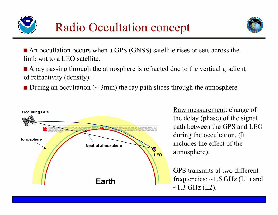
Raw measurement: change of
the delay (phase) of the signal
path between the GPS and LEO
during the occultation. (It
includes the effect of the
atmosphere).
GPS transmits at two different
frequencies: ~1.6 GHz (L1) and
~1.3 GHz (L2).
!! An occultation occurs when a GPS (GNSS) satellite rises or sets across the
limb wrt to a LEO satellite.
!! A ray passing through the atmosphere is refracted due to the vertical gradient
of refractivity (density).
!! During an occultation (~ 3min) the ray path slices through the atmosphere


A few additional words ….
!! The RO occultation technique has three decades of history as a part
of NASA’s planetary exploration missions (e.g. Fjeldbo and
Eshleman, 1969; Fjeldbo et al., 1971; Tyler, 1987; Lindal et al.,
1990; Lindal, 1992) (Mariner IV at Mars, July 1965; Mariner V at
Venus, October 1967)
!! Applying the technique to the Earth’s atmosphere using the GPS
signal was conceived a decade ago (Yunck et al., 1988; Gurvich
and Krasil’nikova, 1990) and demonstrated for the first time with
the GPS/MET experiment in 1995 (Ware et al., 1996).
!! The promises of the technique generated a lot of interest from
several disciplines including meteorology, climatology and
ionospheric physics.

COSMIC (Constellation Observing System
for Meteorology, Ionosphere and Climate)
" ! Joint US-Taiwan mission " ! 6 LEO satellites launched in 15 April 2006 " ! Three instruments:
GPS receiver, TIP, Tri-band beacon
" ! Demonstrate “operational” use of GPS limb sounding with global coverage in near-real time " ! web page: www.cosmic.ucar.edu


COSMIC Launch picture provided by Orbital Sciences Corporation"

Processing of the data

s1, s2,
!1, !2
!"
N
T, Pw, P
Raw measurements of phase of the two signals (L1 and L2)
Bending angles of L1 and L2
(neutral) bending angle
Refractivity
Ionospheric correction
Abel transfrom
Hydrostatic equilibrium,
eq of state, apriori information
Clocks correction,
orbits determination, geometric delay
Overview chart
Atmospheric
products

Bending angle
!! Correction of the clocks errors and relativistic effects on the phase measurements (time corrections).
!! Compute the Doppler shift (change of phase in time during the occultation).
!! Remove the expected Doppler shift for a straight line signal path to get the atmospheric contribution (ionosphere + neutral atmosphere). [The first-order relativistic contributions to the Doppler cancel out].
!! The atmospheric Doppler shift is related to the known position and velocity of the transmitter and receiver (orbit determination).
!! However, there is an infinite number of atmospheres that would produce the same atmospheric Doppler. (The system is undetermined)
!! Certain assumption needs to be made on the shape of the atmosphere: local spherical symmetry
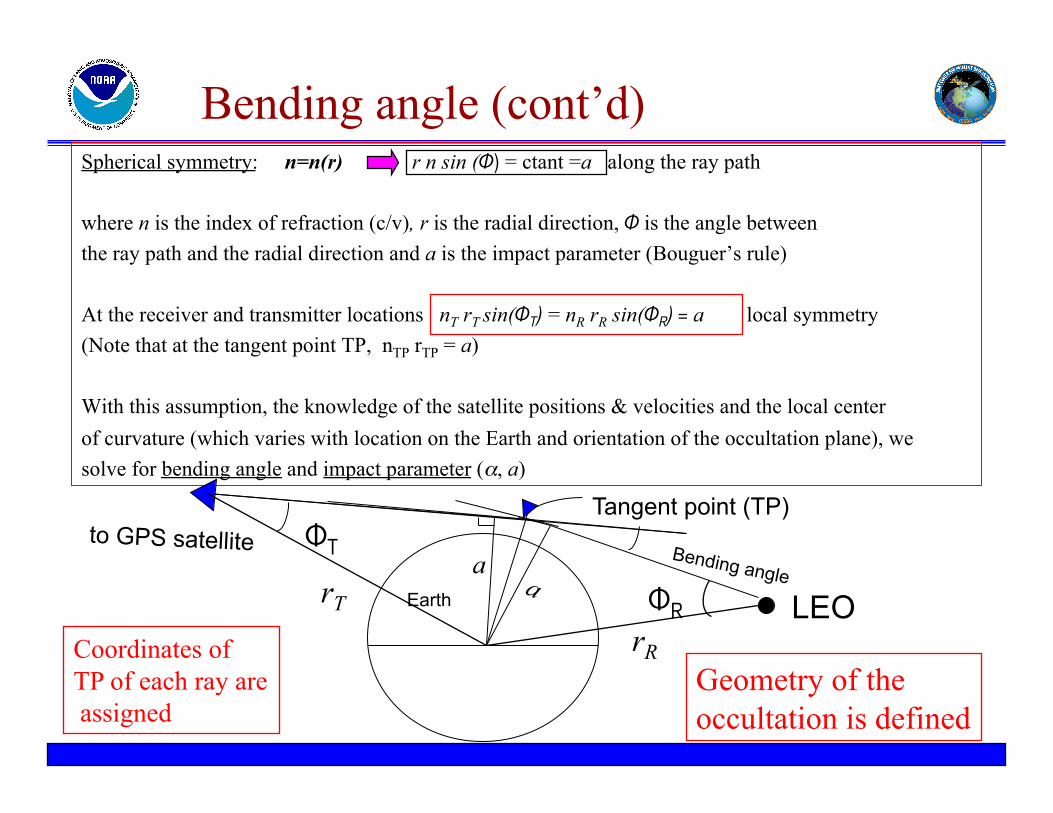
Spherical symmetry: n=n(r) r n sin (!) = ctant =a along the ray path
where n is the index of refraction (c/v), r is the radial direction, ! is the angle between
the ray path and the radial direction and a is the impact parameter (Bouguer’s rule)
At the receiver and transmitter locations nT rT sin(!T) = nR rR sin(!R) = a local symmetry
(Note that at the tangent point TP, nTP rTP = a)
With this assumption, the knowledge of the satellite positions & velocities and the local center
of curvature (which varies with location on the Earth and orientation of the occultation plane), we
solve for bending angle and impact parameter (!, a)
Bending angle
to GPS satellite a
Tangent point (TP)
LEO Earth
!T
!R
Bending angle (cont’d)
rR
rT
Geometry of the
occultation is defined
Coordinates of
TP of each ray are
assigned

(neutral) Bending angle
!! We compute bending angle and impact parameter for each GPS
frequency (!1,a1) and (!2,a2). [The two rays travel slightly
different paths because the ionosphere is dispersive].
!! For neutral atmospheric retrievals, we compute linear combination
of !1 and !2 to remove the first-order ionospheric bending (~1/f2)
and get the ‘neutral’ bending angle !(a)
–! The correction should not be continued above ~50-90km because the
signature of the neutral atmosphere might be comparable to the residual
ionospheric effects.
–! For ionospheric retrievals, the bending from each frequency is used above 60
km.
!! Retrieval: profile of !(a) during an occultation (~ 3,000 rays!)

Refractivity
!! Under (global) spherical symmetry, a profile of !(a) can be inverted (through an Abel inversion) to recover the index of refraction at the tangent point (ie. we reconstruct the atmospheric refractivity)
!! Profile of !(a) is extrapolated above ~60 km (up to ~150 km) using climatology information (through statistical optimization) to solve the integral. (The effects of climatology on the retrieved profile are negligible below ~30 km).
!! Tangent point radius are converted to geometric heights z (ie. heights above mean-sea level geoid).
!! Index of refraction is converted to refractivity: N= 106 (n-1)
!! Retrieval: profile of N(z) during an occultation (~ 3,000 rays)
!
n(rTP) = exp 1/"
#(a)
(a2 $ a1
2)1/ 2da
a1
%
&'
( ) )
*
+ , ,
nrTP
= a1

Rationale for Abel inversion
ray
a
rTP
!
"(a) = #2ad lnn
dr
(n2r2 # a2)1/ 2
dr
rTP
$
%
r
spherical
symmetry
Contribution of different layers to a single
bending angle:
!
n(rTP) = exp 1/"
#(a)
(a2 $ a1
2)1/ 2da
a1
%
&'
( ) )
*
+ , ,
nrTP
= a1Larger contribution when larger gradient
and closer to rTP -> integral peaks at rTP
atmospheric layer

Real world….
!! If the spherical symmetry assumption was exactly true (ie. no horizontal
gradients of refractivity, refractivity only dependent on radial direction)
–! we would not have a job on this business (no weather!)
–! Abel transform would exactly account for and unravel the contributions of the
different layers in the atmosphere to a single bending angle.
!! However, there is a 3D distribution of refractivity (or 2D) that contributes to a
single bending angle and only 1D bending angle (undetermined problem).
[Different from the usual nadir-viewing soundings].
!! There is contribution from the horizontal gradients of refractivity to a single
bending angle. (This can be significant in LT).
!! Abel inversion does not account for these contributions along the ray path so
there is some residual mapping of non-spherical horizontal structure into the
refractivity profile
!! We can think of an “along-track” distribution of the refractivity around the TP.
TP TP
ray ray

Atmospheric variables
!! At microwave wavelengths (GPS), the dependence of N on atmospheric variables can be expressed as:
!
N = 77.6P
T+ 3.73"10
5 Pw
T2# 40.3"10
6 ne
f2
+O(1
f3) +1.4 "Ww + 0.6 "Wi
Hydrostatic balance
P is the total pressure (mb)
T is the temperature (K)
Scattering terms
Ww and Wi are the liquid
water and ice content (gr/m3)
Moisture
Pw is the water vapor
pressure (mb)
Ionosphere
f is the frequency (Hz)
ne electron density(m-3)
–! important in the troposphere for
T> 240K
–! can contribute up to 30% of the
total N in the tropical LT.
–! can dominate the bending in the
LT.
Contributions from liquid water &
ice to N are very small and the
scattering terms can be neglected
RO technology is almost
insensitive to clouds.

Atmospheric variables
~ 70 km
hei
ght
of
tangen
t poin
t
ionospheric term dominates
and the rest of the contributions
can be ignored. N directly
corresponds to electron density
ionosphere
neutral
atmosphere
(hydrostratic
term dominates)
the ionospheric correction removes the
1st order ionospheric term (1/f2) because
GPS has two frequencies.
“wet” atmosphere (P,T, Pw)
“dry” (Pw~ 0) atmosphere
P and T
~ 6 km

“Dry” atmosphere: P and T
!! Where the contribution of the water vapor to the refractivity can be neglected (T< 240K) the expression for N gets reduced to pure density (and P=Pd),
!! + equation of state:
!! + hydrostatic equilibrium
!! Given a boundary condition (eg. P=0 at 150 km), one can derive
–! Profiles of pressure
–! Profiles of temperature (from pressure and density)
–! Profiles of geopotential heights from the geometric heights (RO provides independent values of pressure and height).
!
N(z) = 77.6P(z)
T(z)
!
"(z) =N(z)m
77.6R
!
"P
"z= #g(z)$(z)
with m=mean molecular mass of dry air
R=gas constant

“Dry” atmosphere: P and T (cont’d)
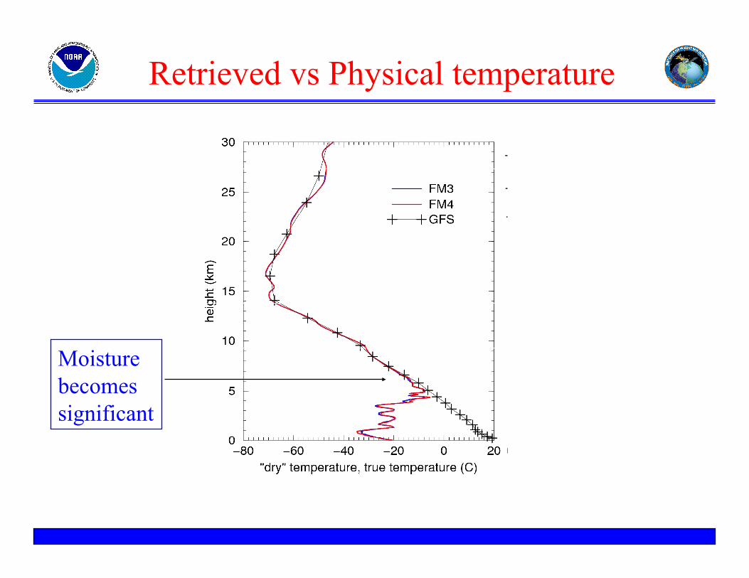
!! When there is no moisture in the atmosphere, the profiles of P and T retrieved
from N correspond to the real atmospheric values.
!! But when there is moisture in the atmosphere, the expression
will erroneously map all the N to P and T of a dry atmosphere.
!! In other words, all the water vapor in the real atmosphere is replaced by dry
molecules that collectively would produce the same amount of N.
!! As a consequence, the retrieved temperature will be lower (cooler) than the real
temperature of the atmosphere
!! Within the GPS RO community, these profiles are usually referred to “dry
temperature” profiles.
!
N = 77.6P
T
!! This is confusing and misleading…
!! I agree!!!
Retrieved vs Physical temperature
Moisture
becomes
significant
“Wet” atmosphere: mass and moisture
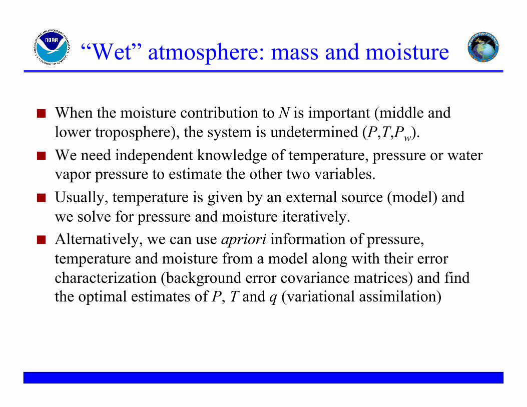
!! When the moisture contribution to N is important (middle and
lower troposphere), the system is undetermined (P,T,Pw).
!! We need independent knowledge of temperature, pressure or water
vapor pressure to estimate the other two variables.
!! Usually, temperature is given by an external source (model) and
we solve for pressure and moisture iteratively.
!! Alternatively, we can use apriori information of pressure,
temperature and moisture from a model along with their error
characterization (background error covariance matrices) and find
the optimal estimates of P, T and q (variational assimilation)
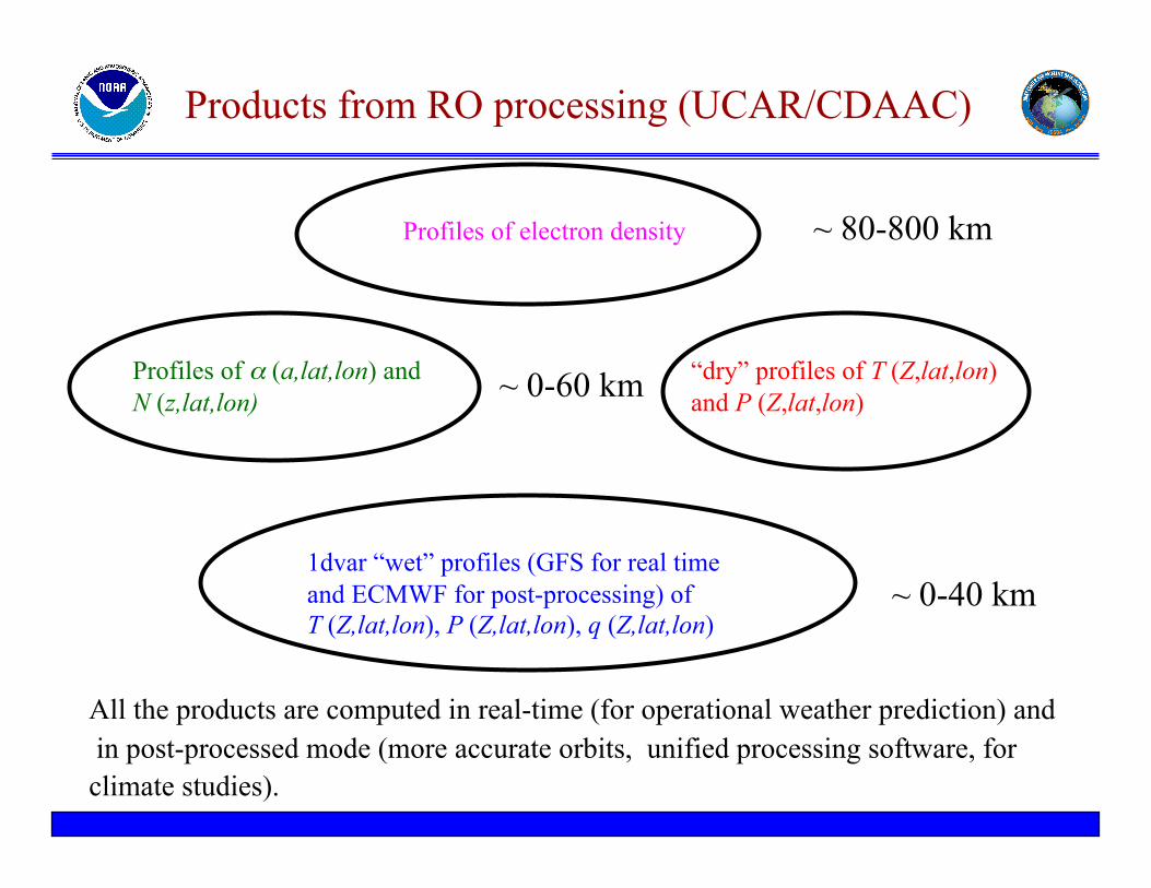
Products from RO processing (UCAR/CDAAC)
All the products are computed in real-time (for operational weather prediction) and
in post-processed mode (more accurate orbits, unified processing software, for
climate studies).
Profiles of electron density
Profiles of ! (a,lat,lon) and
N (z,lat,lon)
~ 80-800 km
~ 0-60 km “dry” profiles of T (Z,lat,lon)
and P (Z,lat,lon)
1dvar “wet” profiles (GFS for real time
and ECMWF for post-processing) of
T (Z,lat,lon), P (Z,lat,lon), q (Z,lat,lon) ~ 0-40 km

Recent improvements
and current challenges

Recent improvements with COSMIC
!! Receiver software: Phase-locked loop tracking Open Loop tracking
–! No tracking errors (we can track down to the surface, OL records the spectrum)
!! Processing software: radio-holographic (RH) methods
–! No problems associated to the processing under multipath (ie. when more than one ray arrive at the receiver at the same time).
»! When multipath occurs, bending cannot be derived from Doppler shift (! is multi-evaluated on a)
»! RH methods allow to distinguish between the different ray paths (!i , ai) under the assumption of spherical symmetry
»! RH methods are applied to L1 signal when L2 is discarded (between ~8 and 20 km)
»! RH methods use phase and amplitude
LEO
The different rays sample
different sections of the
atmosphere

The Effect of Open Loop Tracking
Most profiles didn’t make it to the ground….. Now they do!
C. Rocken (UCAR)

Challenges
!! Non-spherical symmetry
–! Remember: spherical symmetry is needed because otherwise we can’t
»! recover (! , a) from Doppler shift (! is a multi-evaluated function of a)
»! Invert profiles of (! , a) to get profiles of (N , z)
–! Horizontal gradients of refractivity will affect the retrieval of bending angles
(less) and refractivities (more)
!! Turbulence, strong convection, noise
!! Super-refraction conditions
–! Super-refraction occurs when the vertical gradient of N within a layer is so large
(layer of super-refraction) than the ray bends down to the surface.
–! This is not a problem for (! , a)
–! This is a problem when retrieving N(rTP) through Abel inversion (small negative
bias)

No Calibration,
No instrument drift
Calibration,
instrument drift

Uniqueness of RO technique
!! Most measurements are based on physical devices that are not
perfect and usually deteriorate with time. They usually drift and
need to be calibrated.
!! Radio Occultation technique is based on time delays, traceable to
an absolute SI base unit.
!! The raw measurement is not based on a physical device that
deteriorates with time.
!! There is no need for calibration
!! There is no drift
!! There is no instrument-to-instrument bias

Comparison of collocated Profiles
C. Rocken (UCAR)

First collocated ionospheric profiles
From presentation by S. Syndergaard,
UCAR/COSMIC

precision, accuracy,
resolution
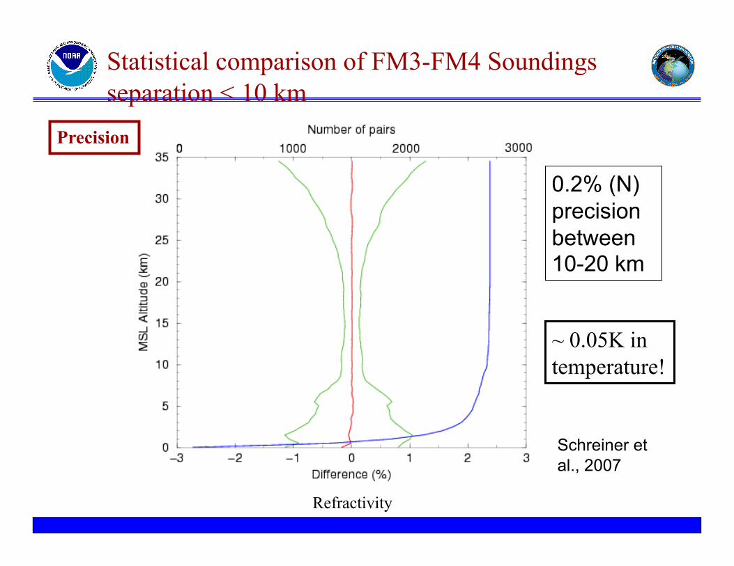
Statistical comparison of FM3-FM4 Soundings
separation < 10 km
Schreiner et
al., 2007
0.2% (N)
precision
between 10-20 km
~ 0.05K in
temperature!
Precision
Refractivity

COSMIC vs GFS statistics for March 2008
!! Accuracy is more difficult to
evaluate
–! difficult to find other instruments as precise (eg. GFS performance changes with season, latitude range, atmospheric phenomena….)
–! Each instrument has its own error characteristics
!! Accuracy of RO is ~ 0.5% in N and ~ 0.5 K in T between ~7-25 km; better than ~ 2 mb rms error (~ 0.5 mb bias) in Pw
Accuracy

“across-track” resolution of an RO ray
!! Bending angle is created by the contribution of the different atmospheric layers (vertical gradient of refractivity).
!! Given a TP, the layer that contributes the most is the one at TP (closest point to the Earth surface and exponential behavior or refractivity).
!! For each TP, we can compute the maximum layer interval that contributes a certain percentage to the bending.
!! The vertical height above the TP that contributes 50% of the bending can be interpreted as vertical resolution of the bending of that single ray (hereafter, resolution of an RO ray).
!! Remember we have 3,000 rays per RO!!
TP ray

ray
a
rTP
r
atmospheric layer that contributes 50% of the bending
Z varies typically from 1-2 km (~ 500 m when strong inversion)
(Kurskinski et al., 1997). The resolution varies between the 3,000
rays because the atmospheric structure which affects the propagation
of the signal changes ray to ray.
Z

Real “across-track” RO resolution
!! GPS RO samples at very high rate (~ 3,000 rays in ~ 3 minutes)
so the vertical resolution will be limited by diffraction (first
Fresnel zone) (~ 100 m LT to ~ 1km in stratosphere). It’s the
‘thickness’ of GO ray.
!! RH methods (diffraction correction algorithms) allow sub-Fresnel
resolution at ~100 m in the whole vertical range.

“along-track” resolution of an RO ray
!! Analogously, the bending contribution of the different atmospheric layers can be written in terms of the distance along the ray path under spherical symmetry.
!! Assuming that N varies exponentially and has a scale height of ~ 6-8 km, the bending contribution along the ray path follows a Gaussian distribution and 50% of the bending is within ~ ± 200 km of TP (Melbourne et al. 1994).
!! Therefore, the information content is not averaged equally along the horizontal extension of the ray path.
!! This has been interpreted as horizontal resolution, but it’s not entirely accurate
ray
a
rTP
r
H

Spatial resolution of a single RO ray
~ 4 times the volumetric
resolution of an AMSU-B
sounder
L~ 100 - 300 km
Z ~ 0.1-1 km
D ~ 1 km
Anthes et al., 2001
2km
15km
TP

Real spatial RO resolution (~3,000 rays)
!! How well RO technology can resolve structures will depend on
(1) spatial resolution of a single ray and (2) density or number of
rays.
!! GPS RO samples at very high rate (~3,000 rays in ~ 3 minutes) so
the density in the vertical direction and in the horizontal direction
that the TP is moving is very high.
!! Horizontal resolution can be improved by increasing the density
of occultations by deploying more LEOs and/or by trading off
temporal resolution versus spatial resolution.

Spatial resolution of a RO
An occultation is not just a vertical profile. The relative motion
of the satellites involves an inclination away from the vertical of the
surface swept out by the occulting rays (a surface, moreover, that
is not in general even a plane)
TP1
TP2
TP4
TP3
TP2
TP1
TP3
1D We need to think in 3D
100-300 km
0.1-1km 1km
ray 2
ray 1
ray 3
ray 4
3,000 rays!!!!
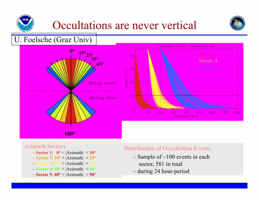
Occultations are never vertical
180°
0°
Azimuth Sectors
– Sector 1: 0° < |Azimuth| < 10°
– Sector 2: 10° < |Azimuth| < 20°
– Sector 3: 20° < |Azimuth| < 30°
– Sector 4: 30° < |Azimuth| < 40°
– Sector 5: 40° < |Azimuth| < 50°
15° 25° 35°
45°
Distribution of Occultation Events
– Sample of ~100 events in each
sector, 581 in total
– during 24 hour-period
U. Foelsche (Graz Univ)

Radio Occultation features summary
!! Limb sounding geometry complementary to ground and space nadir viewing instruments –! High vertical resolution (~100 m)
–! Lower ‘along-track’ resolution (~200 km)
!! All weather-minimally affected by aerosols, clouds or precipitation
!! High accuracy (equivalent to ~ 0.5 Kelvin from ~7-25 km)
!! Equivalent accuracy over ocean than over land
!! No instrument drift, no need for calibration
!! Global coverage
!! No satellite-to-satellite measurement bias
!! Inexpensive compared to other sensors

Assimilation of RO
products at NOAA/
JCSDA
~ 2,000-2,500
soundings/day

Assimilation of RO data
!!The goal is to extract the maximum information content
of the RO data, and to use this information to improve
analysis of model state variables (u, v, T, q, P, …etc) and
consequent forecasts.
!!RO data (bending angles, refractivity, …) are non-
traditional meteorological observations (e.g., wind,
temperature, moisture).
!!The ray path limb-sounding characteristics are very
different from the traditional meteorological measurements
(e.g., radiosonde) or the nadir-viewing passive MW/IR
measurements.
!!Basic rule: the rawer the observation is, the better.

Variational assimilation of RO data
!! In Variational Analysis (e.g. 3D- or 4D-VAR), we minimize the cost function:
!! where x is the analysis vector, xb is the background vector, y0 is the
observation vector, (O+F) is the observation error covariance matrix (F is the
representativeness error) and B is the background error covariance matrix.
!! H is the forward model (observation operator) which transforms the model
variables (e.g. T, u, v, q and P) to the observed variable (e.g. radiance, bending
angle, refractivity, or other observables).
!! We first need to decide what do we want to assimilate
J(x)=(x-xb)TB-1(x-xb)+(y0-H(x))T(O+F)-1(y0-H(x))
analysis Background +
errors + dynamics Observations + errors

s1, s2,
!1, !2
!"
N
T, Pw, P
Raw measurements of phase of the two signals (L1 and L2)
Bending angles of L1 and L2
(neutral) bending angle
Refractivity
Ionospheric correction
Abel transfrom
Hydrostatic equilibrium,
eq of state, apriori information
Clocks correction,
orbits determination, geometric delay
choice of ‘observations’
Atmospheric
products

Choice of observation operators C
om
ple
xit
y!
L1, L2 phase!
L1, L2 bending angle!
Neutral atmosphere bending angle (ray-tracing) !
Linearized nonlocal observation operator (distribution around TP)!
Local refractivity, Local bending angle (single value at TP)!
Retrieved T, q, and P!
Not practical!
Not good enough!
Possible choices!

!! The JCSDA developed, tested and incorporated into the new generation of NCEP’s Global Data Assimilation System the necessary components to assimilate two different type of GPS RO observations (refractivity and bending angle). These components include:
–! complex forward models to simulate the observations (refractivity and bending angles) from analysis variables and associated tangent linear and adjoint models
–! Quality control algorithms & error characterization models
–! Data handling and decoding procedures
–! Verification and impact evaluation algorithms
Achievements at the JCSDA
Cucurull et al., 2007 and 2008

Forward Model for refractivity
!! (1) Geometric height of observation is converted to geopotential height.
!! (2) Observation is located between two model levels.
!! (3) Model variables of pressure, (virtual) temperature and specific humidity are interpolated to observation location.
!! (4) Model refractivity is computed from the interpolated values.
!! The assimilation algorithm produces increments of –! surface pressure
–! water vapor of levels surrounding the observation
–! (virtual) temperature of levels surrounding the observation and all levels below the observation (ie. an observation is allowed to modify its position in the vertical)
!! QC of the data based on the statistics of a month comparison between observations and model simulations of N
!! Errors for N have been tuned to account for representativeness error
!
N = 77.6P
T+ 3.73"10
#5 Pw
T2

Forward Model for bending angle
!! Make-up of the integral:
–! Change of variable to avoid the singularity
–! Choose an equally spaced grid to evaluate the integral by applying the
trapezoid rule
!
x = a2
+ s2
)(
)(
ln
2)(2/122
nrx
dxax
dxnd
aaa
=
!"
"=#
$

!! Compute model geopotential heights and refractivities at the location of the observation
!! Convert geopotential heights to geometric heights
!! Add radius of curvature to the geometric heights to get the radius: r
!! Convert refractivity to index of refraction: n
!! Get refractional radius (x=nr) and dln(n)/dx at model levels and evaluate them in the new grid. We make use of the smoothed Lagrange-polynomial interpolators to assure the continuity of the FM wrt perturbations in model variables.
!! Evaluate the integral in the new grid.
!! QC of the data based on the statistics of a month comparison (same period as used for N) between observations and model simulations of BA
!! Errors for BA have been tuned to account for representativeness.
Forward Model for bending angle (cont’d)

Impact experiments
& operational use of
GPS RO observations
at NCEP

Pre-operational implementation run
!! PRYnc (assimilation of operational obs ),
!! PRYc (PRYnc + COSMIC refractivity)
!! We assimilated around 1,000 COSMIC profiles per day
Anomaly correlation as a function of forecast day (geopotential height)
rms error
(wind)
Cucurull and Derber, 2008
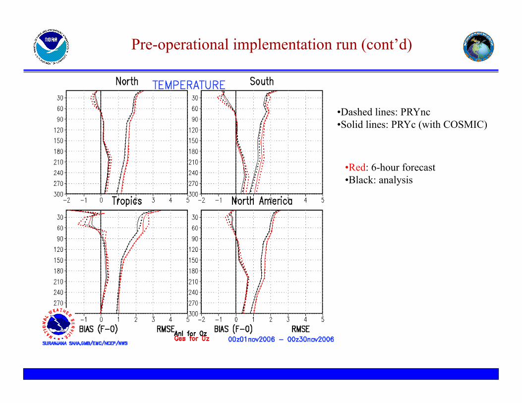
•!Dashed lines: PRYnc
•!Solid lines: PRYc (with COSMIC)
•!Red: 6-hour forecast
•!Black: analysis
Pre-operational implementation run (cont’d)
!! Pre-operational implementation runs showed a positive impact in model skill when COSMIC profiles were assimilated on top of the conventional/satellite observations.
!! As a result, COSMIC became operationally assimilated at NCEP on 1 May 2007, along with the implementation of the new NCEP’s Global Data Assimilation System (GSI/GFS). [Profiles of refractivity were selected for implementation in operations, while the tuning of the assimilation of bending angles will be analyzed at JCSDA soon].
!! The assimilation of observations from the COSMIC mission into the NCEP’s operational system has been a significant achievement of the JCSDA. [Operational assimilation one year after launch!].
COSMIC operational

COSMIC observations at NCEP
0
500
1000
1500
2000
profiles received at NCEP in time for
operations
October
November
December
0%10%20%
30%40%50%60%70%80%90%
100%
obs assimilated (%)
October
November
December
Average COSMIC counts/day at NCEP (2007)
!! We assimilate rising and setting occultations, there is no black-listing of the low-level
observations (provided they pass the quality control checks), and we do not assimilate
observations above 30 km (due to model limitations).
!! In an occultation, the drift of the tangent point is considered.
The remaining 20% received, but not assimilated, is due to:
–! Preliminary quality control checks (bad data/format)
–! Gross error check
–! Statistics quality control check (obs too different from the model-obs statistics)

Recent impacts with COSMIC
!! expx (NO COSMIC)
!! cnt (operations - with COSMIC)
!! exp (updated RO assimilation code - with COSMIC)
COSMIC provides 8
hours of gain in
model forecast skill
at day 4!!!!
Cucurull, 2009

Summary and outlook
!! NCEP has been successfully assimilating GPS RO observations
into it’s Global Data Assimilation System since 1 May 2007
!! Results indicate that GPS RO observations contain unique
information on the atmospheric state of the atmosphere (high
accuracy, high vertical resolution, very small systematic difference
vs. model compared to other satellite data, global coverage, all
weather conditions, …)
!! Future work within the DA community is focusing on improving
the forward operators for GPS RO measurements (capability to
assimilate rawer products, account for horizontal gradients of
refractivity, …)

If someone is interested on this subject … the JCSDA has a 1-2 yr
post-doc position available to work on Observing System
Simulation Experiments (OSSEs) with GPS RO data.
Talk to me or send me an email: [email protected]